an uav and satellite multispectral data approach to

remote sensing

Article

An UAV and Satellite Multispectral Data Approach toMonitor Water Quality in Small Reservoirs

Carmen Cillero Castro 1,*, Jose Antonio Domínguez Gómez 2, Jordi Delgado Martín 3 ,Boris Alejandro Hinojo Sánchez 1, Jose Luis Cereijo Arango 3, Federico Andrés Cheda Tuya 1 andRamon Díaz-Varela 4

1 R&D Department, 3edata Environmental Engineering L. C., 27004 Lugo, Spain;[email protected] (B.A.H.S.); [email protected] (F.A.C.T.)

2 Departamento de Física Matemática y de Fluidos, Facultad de Ciencias, Universidad Nacional de Educacióna Distancia (UNED), 28040 Madrid, Spain; [email protected]

3 Civil Engineering School, University of A Coruña, 15008 A Coruña, Spain; [email protected] (J.D.M.);[email protected] (J.L.C.A.)

4 Botany Department, Higher Politechnic School, GI-1809-BIOAPLIC, University of Santiago de Compostela,27002 Lugo, Spain; [email protected]

* Correspondence: [email protected]; Tel.: +34-982-284-150

Received: 7 March 2020; Accepted: 5 May 2020; Published: 9 May 2020��

Abstract: A multi-sensor and multi-scale monitoring tool for the spatially explicit and periodicmonitoring of eutrophication in a small drinking water reservoir is presented. The tool was builtwith freely available satellite and in situ data combined with Unmanned Aerial Vehicle (UAV)-basedtechnology. The goal is to evaluate the performance of a multi-platform approach for the trophicstate monitoring with images obtained with MultiSpectral Sensors on board satellites Sentinel 2(S2A and S2B), Landsat 8 (L8) and UAV. We assessed the performance of three different sensors(MultiSpectral Instrument (MSI), Operational Land Imager (OLI) and Rededge Micasense) forretrieving the pigment chlorophyll-a (chl-a), as a quantitative descriptor of phytoplankton biomassand trophic level. The study was conducted in a waterbody affected by cyanobacterial blooms, oneof the most important eutrophication-derived risks for human health. Different empirical modelsand band indices were evaluated. Spectral band combinations using red and near-infrared (NIR)bands were the most suitable for retrieving chl-a concentration (especially 2 band algorithm (2BDA),the Surface Algal Bloom Index (SABI) and 3 band algorithm (3BDA)) even though blue and greenbands were useful to classify UAV images into two chl-a ranges. The results show a moderatelygood agreement among the three sensors at different spatial resolutions (10 m., 30 m. and 8 cm.),indicating a high potential for the development of a multi-platform and multi-sensor approach forthe eutrophication monitoring of small reservoirs.

Keywords: satellite; water quality; multispectral imagery; UAV; eutrophication; monitoring

1. Introduction

One of the main problems currently affecting water resources is the eutrophication of waterbodies, both coastal and freshwater [1,2]; it was already known ten years ago that around 20% ofEuropean lakes were suffering from nutrient enrichment [3]. In the European Union, the managementof reservoirs and natural waterbodies is directly linked to the Water Framework Directive [4], whichrequires periodic monitoring; this being a common trait all over the world [5]. Most of the reservoirmonitoring programs are currently based on measurements taken in the field making it difficultto capture the spatial and temporal variability of phenomena such as algal blooms, with irregular

Remote Sens. 2020, 12, 1514; doi:10.3390/rs12091514 www.mdpi.com/journal/remotesensing

http://www.mdpi.com/journal/remotesensing

http://www.mdpi.com

https://orcid.org/0000-0002-8261-8087

https://orcid.org/0000-0001-6094-2153

http://www.mdpi.com/2072-4292/12/9/1514?type=check_update&version=1

http://dx.doi.org/10.3390/rs12091514

http://www.mdpi.com/journal/remotesensing

Remote Sens. 2020, 12, 1514 2 of 33

spatiotemporal patterns and potential toxicity (Cyanobacterial blooms). This circumstance hampersthe possibility of taking timely and informed management decisions to prevent, counteract or mitigatethe negative effects of eutrophication in drinking water reservoirs where “early warning” systems areincreasingly needed.

The application of remote sensing for the measurement of a range of parameters indicativeof water quality (temperature, transparency, turbidity, concentration of photosynthetic pigments,colored dissolved organic matter, etc.) has been proven effective in capturing this variability in aquaticecosystems through the use of satellite images from multispectral sensors such as a Medium ResolutionImaging Spectrometer (MERIS), the various Landsat Thematic Mapper/Enhanced Thematic Mapper(TM/ETM+), Operational Land Imager (OLI) sensors, or more recently Sentinel 2 MSI (e.g., [6–14]).

The retrieval of phytoplankton chlorophyll-a concentration (chl-a) from remotely sensed data isone of the key issues in aquatic remote sensing. The spectral signature of chl-a is characterized bystrong absorption in the blue (443 nm) and red wavelengths (near 675 nm) and high reflectance in thegreen (550–555 nm) and rededge spectrum regions (685–710 nm) [15–17]. These spectral features havebeen used to develop several band ratios to quantify chl-a concentration in inland and near-coastaltransitional waters through empirical approaches, providing timely and accurate information [9].Specifically, empirical algorithms based on green and blue bands have been successfully applied toopen oceans (Case 1 waters [18]) and oligotrophic inland waters [19,20], while the near-infrared (NIR)to red reflectance ratios are used in productive waters (Case 2). In the latter, chl-a is not correlatedwith the other optically active constituents, and the absorption by Coloured Dissolved Organic Matter(CDOM), tripton, and other pigments overlaps the absorption peak of chl-a in the blue spectral region.In this type of water, the only spectral range maximally sensitive to chl-a is the Red-NIR, which is stillaffected by the residual absorption by CDOM and tripton. Several algorithms have been developedusing this spectral range, all based on the properties of the reflectance peak near 700 nm, which ismaximally sensitive to the variations in chl-a in water and its relationships with the red chl-a absorptionband (660–690 nm). Still, the backscattering by all particulate matter is also affecting the reflectance inthis spectral region, hence a third band in the NIR region (>740 nm) was added by [21] to accountfor this effect in chl-a estimation, as the variations in particulate backscattering, control variations inreflectance in this region [21–23]. The use of combined algorithms has been also suggested for themonitoring of these different water types and trophic states [24].

Two of the main limitations that affect the systematic or periodic monitoring of aquatic ecosystemsthrough satellite remote sensing are: on the one hand, the presence of atmospheric effects, which canleave the managers of water bodies without information for extended time periods, and on the otherhand, the spatial resolution of sensors on board satellites. Multispectral sensors designed for waterapplications are mainly designed for ocean water monitoring (e.g., MODerate resolution ImagingSpectroradiometer (MODIS), Medium Resolution Imaging Spectrometer (MERIS) or Ocean and LandColour Instrument (OLCI)) and their coarse spatial resolution is lower than that required to monitorsmall systems. It is for this reason that the sensors currently employed for the monitoring of mostinland water bodies are sensors initially designed for terrestrial applications as Sentinel 2 MultiSpectralInstrument (MSI) and Landsat 8 Operational Land Imager (OLI).

As with the multispectral sensors on board satellites, the commercial technology currently availablefor sensors that can be boarded on UAVs is not specifically designed for aquatic but for terrestrialapplications, mostly for precision agriculture. Hence, the design of the sensor spectral bands is notideal, but theoretically they can be used for some aquatic applications, including the quantification ofthe pigment chl-a.

Based on this background, we propose a methodology for the monitoring of aquatic resourcestrying to maximize the periodicity of data acquisition and gap-filling by combining sensors andplatforms, complementing an established monitoring program. On it, freely distributed imagesobtained through multispectral sensors on board two satellite platforms (Sentinel 2 and Landsat 8),used as a virtual constellation [25,26], are combined with commercial multispectral sensors mounted on

Remote Sens. 2020, 12, 1514 3 of 33

UAV platforms. This approach is seeking to combine the affordability, stability, quality and continuityof ESA and NASA missions with the flexibility and spatial resolution provided by the use of UAVplatforms, to make the most of these resources in favor of efficient management of aquatic resources.The empirical approach has been used to test the retrieval of chl-a as a quantitative descriptor of thepresence of phytoplankton and the degree of eutrophication of a small water body, using images atdifferent scales taken with three multispectral sensors with different characteristics, in a test carried outduring 2017 and 2018 in a drinking water reservoir regularly affected by the presence of cyanobacteria.

The objectives of the study are: (1) To evaluate the performance of different algorithms and bandindices in a small waterbody, by using images obtained with three different sensors, during 2016,2017 and 2018. (2) To validate the application of free-distributed multispectral images from Sentinel2 and Landsat 8 satellites to improve the continuous monitoring of small reservoirs, in an area ofvery high cloud cover (Galicia, NW Iberian Peninsula). (3) To assess the detection and quantificationcapability for chl-a of a remote sensing system consisting of a commercial multispectral camera onboard a multirotor UAV and to verify its potential application in the absence of valid satellite images.

2. Materials and Methods

2.1. Study Area

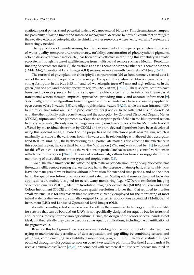
The study area is a small reservoir (4.5 ha) with a capacity of 0.24 hm3 located in Spain, in thenorthwest (NW) of the Iberian Peninsula (Figure 1). Since 2000, the reservoir has maintained adrinking water supply service for households and facilities in the municipality. According to the dataobtained during the conducted sampling, it has a maximum depth of 9.0 m. A river park was setup in 2012, when the reservoir also became navigable and a small jetty and a recreational area wereinstalled, confirming its use as a leisure area for residents. The reservoir is located in the AtlanticBiogeographical Region, under an oceanic temperate climate, with a mean annual temperature of19.6 ◦C and high precipitation (1146.2 mm) and relative humidity (90.6%) (mean annual values for fiveyears (2013–2017) [27]). The rainiest period spans from November to February.

Remote Sens. 2020, 12, x FOR PEER REVIEW 4 of 33

Figure 1. Localization of the study site in Europe (A), in the NW of the Iberian Peninsula (B) and aerial picture of the reservoir with in situ sampling points both from the periodic monitoring [28] and from the two Unmanned Aerial Vehicle (UAV) flights (same sampling points for 2017 and 2018) (C).

2.2. In Situ Data

The in situ chl-a data used to calibrate and validate the satellite models were taken from the Galician Platform for Environmental Information (GAIA), supplied freely and on a regular basis, coming from the cyanobacterial monitoring program in the reservoirs of the district [28]. It maintains 2 permanent sampling points in the waterbody, one close to the dock (BP) and the other near the uptake system for drinking water (BC) (Figure 1). For the purpose of this study, we established two matchup points for the satellite reflectance data retrieval, as near as possible as these two ones, in a place still considered representative of the chl-a values, while far enough from the dock and the wall dam to be as unaffected as possible from adjacency effects. The point near the dock (BP) is located in the direction of dominant winds and tends to accumulate a high concentration of cyanobacteria during bloom events. Under such conditions, this point was not considered representative of the free water pixel used for matchup with satellite images and not used in the study.

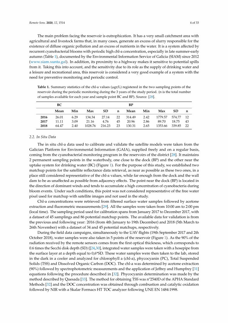
Table 1. Summary statistics of the chl-a values (μgr/l) registered in the two sampling points of the reservoir during the periodic monitoring during the 3 years of the study period. (n is the total number of samples available for each year and sample point BC and BP). Source: [28].

BC BP Mean Min Max SD n Mean Min Max SD n

2016 26.01 6.29 134.34 27.14 22 314.49 2.42 1779.57 574.77 12 2017 11.11 3.09 21.16 4.76 45 20.96 2.86 89.70 18.75 43 2018 64.47 2.40 1028.76 216.23 23 130.31 2.65 1353.66 339.85 22

Figure 1. Localization of the study site in Europe (A), in the NW of the Iberian Peninsula (B) and aerialpicture of the reservoir with in situ sampling points both from the periodic monitoring [28] and fromthe two Unmanned Aerial Vehicle (UAV) flights (same sampling points for 2017 and 2018) (C).

Remote Sens. 2020, 12, 1514 4 of 33

The main problem facing the reservoir is eutrophication. It has a very small catchment area withagricultural and livestock farms that, in many cases, generate an excess of slurry responsible for theexistence of diffuse organic pollution and an excess of nutrients in the water. It is a system affected byrecurrent cyanobacterial blooms with periodic high chl-a concentration, especially in late summer-earlyautumn (Table 1), documented by the Environmental Information Service of Galicia (SIAM) since 2012(www.siam.xunta.gal). In addition, its proximity to a highway makes it sensitive to potential spillsfrom it. Taking this into account, and the sensitivity due to its role as the supply of drinking water anda leisure and recreational area, this reservoir is considered a very good example of a system with theneed for preventive monitoring and periodic control.

Table 1. Summary statistics of the chl-a values (µgr/L) registered in the two sampling points of thereservoir during the periodic monitoring during the 3 years of the study period. (n is the total numberof samples available for each year and sample point BC and BP). Source: [28].

BC BP

Mean Min Max SD n Mean Min Max SD n

2016 26.01 6.29 134.34 27.14 22 314.49 2.42 1779.57 574.77 122017 11.11 3.09 21.16 4.76 45 20.96 2.86 89.70 18.75 432018 64.47 2.40 1028.76 216.23 23 130.31 2.65 1353.66 339.85 22

2.2. In Situ Data

The in situ chl-a data used to calibrate and validate the satellite models were taken from theGalician Platform for Environmental Information (GAIA), supplied freely and on a regular basis,coming from the cyanobacterial monitoring program in the reservoirs of the district [28]. It maintains2 permanent sampling points in the waterbody, one close to the dock (BP) and the other near theuptake system for drinking water (BC) (Figure 1). For the purpose of this study, we established twomatchup points for the satellite reflectance data retrieval, as near as possible as these two ones, in aplace still considered representative of the chl-a values, while far enough from the dock and the walldam to be as unaffected as possible from adjacency effects. The point near the dock (BP) is located inthe direction of dominant winds and tends to accumulate a high concentration of cyanobacteria duringbloom events. Under such conditions, this point was not considered representative of the free waterpixel used for matchup with satellite images and not used in the study.

Chl-a concentrations were retrieved from filtered surface water samples followed by acetoneextraction and fluorometric measurements [29]. All the samples were taken from 10:00 am to 2:00 pm(local time). The sampling period used for calibration spans from January 2017 to December 2017, witha dataset of 45 samplings and 86 potential matchup points. The available data for validation is fromthe previous and following year: 2016 (from 4th January to 19th December) and 2018 (5th March to26th November) with a dataset of 34 and 45 potential matchups, respectively.

During the field data campaigns, simultaneously to the UAV flights (19th September 2017 and 2thOctober 2018), water samples were also taken in 5 points of the reservoir (Figure 1). As the 90% of theradiation received by the remote sensors comes from the first optical thickness, which corresponds to0.6 times the Secchi disk depth (SD) ([24,30], integrated water samples were taken with a hosepipe fromthe surface layer at a depth equal to 0,6*SD. These water samples were then taken to the lab, storedin the dark in a cooler and analyzed for chlorophyll a (chl-a), phycocyanin (PC), Total SuspendedSolids (TSS) and Dissolved Organic Carbon (DOC). The chl-a was determined by acetone extraction(90%) followed by spectrophotometric measurements and the application of Jeffrey and Humpfrey [31]equations following the procedure described in [32]. Phycocyanin determination was made by themethod described by Quesada [33]. The method for obtaining TSS was nº2540D of the APHA StandardMethods [32] and the DOC concentration was obtained through combustion and catalytic oxidationfollowed by NIR with a Skalar Formacs HT TOC analyzer following UNE EN 1484:1998.

www.siam.xunta.gal

Remote Sens. 2020, 12, 1514 5 of 33

Five profiles were also done with a YSI6600 multi parameter sonde with the following attachedsensors: temperature (◦C), electrical conductivity (µS/cm.), pH/ORP, dissolved oxygen (% and mg/L),turbidity (NTU), chlorophyll (µgr/L) and phycocyanin (BGA-PC, cells/mL). The sample taken inthe central point of the reservoir was also analyzed for principal nutrients (Total PhosphorousTP, Total Nitrogen TN, Nitrate, Nitrite and Ammonium). TP was analyzed by ICP-MS followingan internal procedure of the support services for research (SAI) of the University of A Coruña(nº P-SAI-UEPM-09) accredited by ENAC, with high-resolution equipment (ELEMENTXR/ELEMENT2;Thermo Finnigan). Determination of TN was done through catalytic combustion and chemiluminiscencedetection following prior oxidation with a Skalar Formacs HT analyzer in samples filtered throughmembrane (Millipore Millex-HM, 0.45 µm) following UNE-EN 12260:2004. Colorimetric ammoniumdetermination was performed by AquaKem 250 (Labmedics) in water samples previously filteredthrough Millex-HN membrane (0.45 µm) following SAI internal procedure: P-SAI-UAA-15. Nitrate andnitrite were determined by ionic chromatography with a chromatographer Metrohm 850 ProfessionalIC equipped with a column Metrohm Metrosep A Supp 7 250/4.0 mm, following the internal SAIprocedure: P-SAIUAA-20.

2.3. Remotely Sensed Data

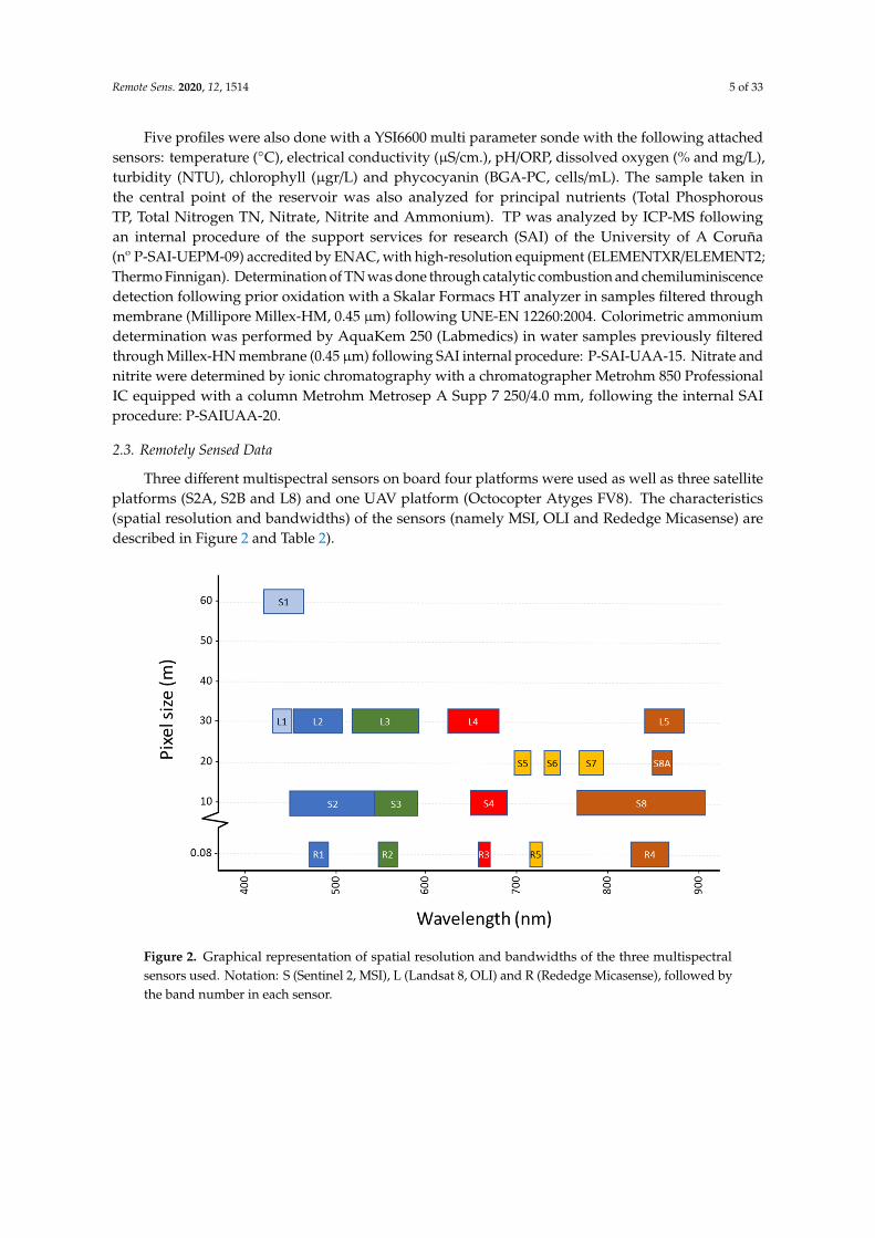
Three different multispectral sensors on board four platforms were used as well as three satelliteplatforms (S2A, S2B and L8) and one UAV platform (Octocopter Atyges FV8). The characteristics(spatial resolution and bandwidths) of the sensors (namely MSI, OLI and Rededge Micasense) aredescribed in Figure 2 and Table 2).


Figure 2. Graphical representation of spatial resolution and bandwidths of the three multispectral sensors used. Notation: S (Sentinel 2, MSI), L (Landsat 8, OLI) and R (Rededge Micasense), followed by the band number in each sensor.

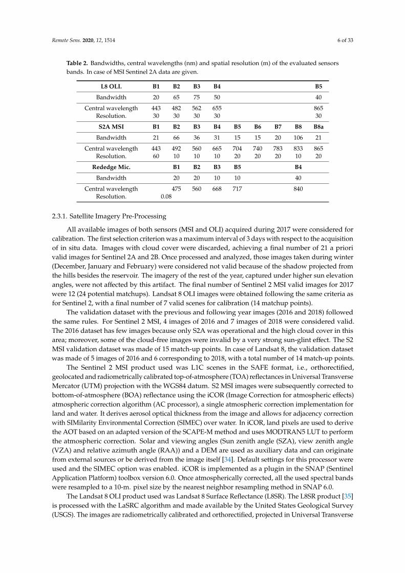
Table 2. Bandwidths, central wavelengths (nm) and spatial resolution (m) of the evaluated sensors bands. In case of MSI Sentinel 2A data are given.

L8 OLI. B1 B2 B3 B4 B5 Bandwidth 20 65 75 50 40

Central wavelength 443 482 562 655 865 Resolution. 30 30 30 30 30 S2A MSI B1 B2 B3 B4 B5 B6 B7 B8 B8a Bandwidth 21 66 36 31 15 15 20 106 21

Central wavelength 443 492 560 665 704 740 783 833 865 Resolution. 60 10 10 10 20 20 20 10 20

Rededge Mic. B1 B2 B3 B5 B4 Bandwidth 20 20 10 10 40

Central wavelength 475 560 668 717 840 Resolution. 0.08

2.3.1. Satellite Imagery Pre-Processing

All available images of both sensors (MSI and OLI) acquired during 2017 were considered for calibration. The first selection criterion was a maximum interval of 3 days with respect to the acquisition of in situ data. Images with cloud cover were discarded, achieving a final number of 21 a priori valid images for Sentinel 2A and 2B. Once processed and analyzed, those images taken during winter (December, January and February) were considered not valid because of the shadow projected from the hills besides the reservoir. The imagery of the rest of the year, captured under higher sun elevation angles, were not affected by this artifact. The final number of Sentinel 2 MSI valid images for 2017 were 12 (24 potential matchups). Landsat 8 OLI images were obtained following the same criteria as for Sentinel 2, with a final number of 7 valid scenes for calibration (14 matchup points).

The validation dataset with the previous and following year images (2016 and 2018) followed the same rules. For Sentinel 2 MSI, 4 images of 2016 and 7 images of 2018 were considered valid. The 2016 dataset has few images because only S2A was operational and the high cloud cover in this area; moreover, some of the cloud-free images were invalid by a very strong sun-glint effect. The S2 MSI validation dataset was made of 15 match-up points. In case of Landsat 8, the validation dataset was made of 5 images of 2016 and 6 corresponding to 2018, with a total number of 14 match-up points.

Figure 2. Graphical representation of spatial resolution and bandwidths of the three multispectralsensors used. Notation: S (Sentinel 2, MSI), L (Landsat 8, OLI) and R (Rededge Micasense), followed bythe band number in each sensor.

Remote Sens. 2020, 12, 1514 6 of 33

Table 2. Bandwidths, central wavelengths (nm) and spatial resolution (m) of the evaluated sensorsbands. In case of MSI Sentinel 2A data are given.

L8 OLI. B1 B2 B3 B4 B5

Bandwidth 20 65 75 50 40

Central wavelength 443 482 562 655 865Resolution. 30 30 30 30 30

S2A MSI B1 B2 B3 B4 B5 B6 B7 B8 B8a

Bandwidth 21 66 36 31 15 15 20 106 21

Central wavelength 443 492 560 665 704 740 783 833 865Resolution. 60 10 10 10 20 20 20 10 20

Rededge Mic. B1 B2 B3 B5 B4

Bandwidth 20 20 10 10 40

Central wavelength 475 560 668 717 840Resolution. 0.08

2.3.1. Satellite Imagery Pre-Processing

All available images of both sensors (MSI and OLI) acquired during 2017 were considered forcalibration. The first selection criterion was a maximum interval of 3 days with respect to the acquisitionof in situ data. Images with cloud cover were discarded, achieving a final number of 21 a priorivalid images for Sentinel 2A and 2B. Once processed and analyzed, those images taken during winter(December, January and February) were considered not valid because of the shadow projected fromthe hills besides the reservoir. The imagery of the rest of the year, captured under higher sun elevationangles, were not affected by this artifact. The final number of Sentinel 2 MSI valid images for 2017were 12 (24 potential matchups). Landsat 8 OLI images were obtained following the same criteria asfor Sentinel 2, with a final number of 7 valid scenes for calibration (14 matchup points).

The validation dataset with the previous and following year images (2016 and 2018) followedthe same rules. For Sentinel 2 MSI, 4 images of 2016 and 7 images of 2018 were considered valid.The 2016 dataset has few images because only S2A was operational and the high cloud cover in thisarea; moreover, some of the cloud-free images were invalid by a very strong sun-glint effect. The S2MSI validation dataset was made of 15 match-up points. In case of Landsat 8, the validation datasetwas made of 5 images of 2016 and 6 corresponding to 2018, with a total number of 14 match-up points.

The Sentinel 2 MSI product used was L1C scenes in the SAFE format, i.e., orthorectified,geolocated and radiometrically calibrated top-of-atmosphere (TOA) reflectances in Universal TransverseMercator (UTM) projection with the WGS84 datum. S2 MSI images were subsequently corrected tobottom-of-atmosphere (BOA) reflectance using the iCOR (Image Correction for atmospheric effects)atmospheric correction algorithm (AC processor), a single atmospheric correction implementation forland and water. It derives aerosol optical thickness from the image and allows for adjacency correctionwith SIMilarity Environmental Correction (SIMEC) over water. In iCOR, land pixels are used to derivethe AOT based on an adapted version of the SCAPE-M method and uses MODTRAN5 LUT to performthe atmospheric correction. Solar and viewing angles (Sun zenith angle (SZA), view zenith angle(VZA) and relative azimuth angle (RAA)) and a DEM are used as auxiliary data and can originatefrom external sources or be derived from the image itself [34]. Default settings for this processor wereused and the SIMEC option was enabled. iCOR is implemented as a plugin in the SNAP (SentinelApplication Platform) toolbox version 6.0. Once atmospherically corrected, all the used spectral bandswere resampled to a 10-m. pixel size by the nearest neighbor resampling method in SNAP 6.0.

The Landsat 8 OLI product used was Landsat 8 Surface Reflectance (L8SR). The L8SR product [35]is processed with the LaSRC algorithm and made available by the United States Geological Survey(USGS). The images are radiometrically calibrated and orthorectified, projected in Universal Transverse

Remote Sens. 2020, 12, 1514 7 of 33

Mercator (UTM) with the WGS84 datum. The L8SR product provides the surface reflectance imagerescaled by a factor of 10,000. This product has been proven effective in aquatic applications [36–38].For both satellite products, surface reflectance data were transformed into Rrs dividing by π.

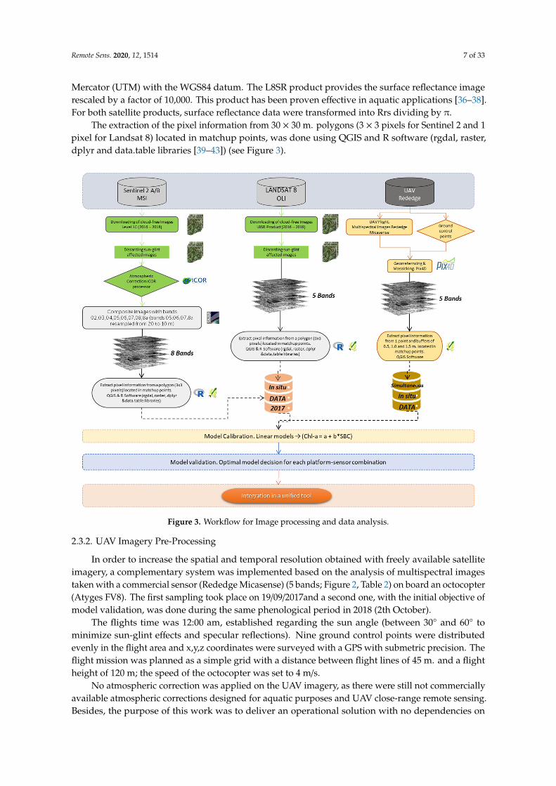
The extraction of the pixel information from 30 × 30 m. polygons (3 × 3 pixels for Sentinel 2 and 1pixel for Landsat 8) located in matchup points, was done using QGIS and R software (rgdal, raster,dplyr and data.table libraries [39–43]) (see Figure 3).


𝑁𝑅𝑀𝑆𝐸 = ´ (5)

𝑀𝐴𝑃𝐸 = 1𝑛 𝑦 − 𝑦𝑦 (6)

𝑏𝑖𝑎𝑠 = ∑ 𝑦 − 𝑦 , (7)

where 𝒚𝒑 is the predicted values, 𝒚𝒎 is the measured values and n is the number of samples.

Figure 3. Workflow for Image processing and data analysis.

3. Results

3.1. Water Quality

The studied reservoir is an eutrophic waterbody with recurrent cyanobacterial blooms since 2012, documented through the Galician Platform for Environmental Information (GAIA) (www.gaia.xunta.es) (Table 1). This periodic monitoring showed during 2017 Microcystis sp. as the dominant cyanobacteria, even though Chorococcus sp., Aphanocapsa sp. and Woronischia sp. were also present. The chl-a reached a maximum in the BC point (which is considered more representative of the main waterbody) of 21.26 µgr/l during May being the mean value for this year in BC sampling point 11.11 µgr/l. The highest cyanobacteria cell concentration was registered in October (9750 cel/ml) being Aphanocapsa sp. the dominant taxa. In the BP sampling point, the maximum chl-a was registered on 25th September (89.70 µgr/l), in this case, Microcystis sp. Being the dominant cyanobacterial taxa (115,500 cel/ml), and the mean annual value 20.96 µgr/l [28]. During 2018 (when the second UAV

Figure 3. Workflow for Image processing and data analysis.

2.3.2. UAV Imagery Pre-Processing

In order to increase the spatial and temporal resolution obtained with freely available satelliteimagery, a complementary system was implemented based on the analysis of multispectral imagestaken with a commercial sensor (Rededge Micasense) (5 bands; Figure 2, Table 2) on board an octocopter(Atyges FV8). The first sampling took place on 19/09/2017and a second one, with the initial objective ofmodel validation, was done during the same phenological period in 2018 (2th October).

The flights time was 12:00 am, established regarding the sun angle (between 30◦ and 60◦ tominimize sun-glint effects and specular reflections). Nine ground control points were distributedevenly in the flight area and x,y,z coordinates were surveyed with a GPS with submetric precision. Theflight mission was planned as a simple grid with a distance between flight lines of 45 m. and a flightheight of 120 m; the speed of the octocopter was set to 4 m/s.

No atmospheric correction was applied on the UAV imagery, as there were still not commerciallyavailable atmospheric corrections designed for aquatic purposes and UAV close-range remote sensing.Besides, the purpose of this work was to deliver an operational solution with no dependencies on

Remote Sens. 2020, 12, 1514 8 of 33

concurrent field radiometric sampling, and therefore the effect of the thin atmosphere layer betweenthe sensor and the water surface was neglected. The georeferencing, radiometric processing andmosaicking of the image were performed with the Pix4D software (Pix4D, Lausanne, Sw.). Rawmultispectral images were corrected to ground absolute reflectance using the irradiance measurestaken along with each snapshot by a specific sensor onboard the UAV and spectrally rescaled against acalibration panel with values around 70 % of diffuse reflectance in the visible-infrared spectrum. Theextraction of the image information was done at different sampling sizes corresponding to the medianof all the pixel values included in circular buffers of 0.5, 1.0 and 1.5 m. around each match-up pointusing QGIS 2.18.15. These buffers were set in order to test the coherence and representativeness of thedata given by the sensor against a different size of sampling areas around the in situ sampling points.

In order to compare the reflectances recorded by the S2 MSI and UAV sensors, we used twosimultaneous images of both sensors (10/02/2018). We made a focal analysis on the Micasense bands inwhich the extent of each of the S2 MSI pixels covering the reservoir was used as focal unit, once filteredthose prone to spectral mixtures from the shore area. From these extents (squares of 10 × 10 m. labelledwith an unique ID), a synthetic value of the Micasense reflectance for each band was calculated asthe mean value of the Micasense image pixels covered by the area of each individual S2 MSI imagepixel extent.

2.3.3. Data Analysis

For developing the empirical model, linear fits were applied expressing the relationships betweenRrs at different wavelengths in every match-up point and their corresponding “in situ” chl-a data as alinear function of the format:

chl-a = a + b × SBC (1)

where a and b are the model parameters (intercept and slope, respectively) and SBC is the testedSpectral Band Combination (Table 3). SBCs are either an index, a ratio or an algorithm. Some of thesecombinations (of two and three bands) are those proposed by different authors and adapted to OLI,MSI and Rededge spectral bands (Figure 2, Table 2).

As shown in Table 3, in addition to the standard 3 bands and 2 bands algorithms (3BDA and2BDA) [21,22], we have included one modification of the 3 bands algorithm (3BDA_MOD) adapted toUAV- Rededge Micasense data.

These both algorithms (2BDA and 3BDA) come from a common initial conceptual model, relatingremotely sensed reflectance and pigment content in vascular plant leaves [44]. The model was initiallyconceived to isolate the absorption coefficient of the pigment of interest from the reflectance spectrum.The 3BDA relationship used between the pigment content in the leaves and the reflectance wasas follows:

3BDA− Pigment concentration ∝(R−1λ1 −R−1

λ2

)Rλ3 (2)

When the 3BDA model is tuned for the retrieval of chl-a in turbid productive waters, as describedby [21,22,45], the spectral regions are defined as:

• λ1: Spectral region such that R−1λ1 is maximally sensitive to the absorption chl-a but still affected

by the absorption of other constituents and backscattering: λ1 = 660–690 nm.• λ2: Spectral region such that R−1

λ2 is minimally sensitive to chl-a for which the absorption byother constituents is almost equal to that at λ1: 710-λ2-730 nm.

• λ3: Spectral region minimally affected by the absorption of pigments, used to compensate for thevariability in backscattering between samples: initially λ3 > 740 nm.

Remote Sens. 2020, 12, 1514 9 of 33

The 2BDA algorithm is described by the authors as a particular case of the 3BDA, which onlyuses the λ1 and λ3 terms of the equation and gives good results when achla(λ1)� bb and achla(λ1)�atripton(λ1)+ aCDOM(λ1) [39], any a being the absorption coefficients and bb the backscattering coefficient.

2BDA− Pigment concentration ∝(R−1λ1

)Rλ3 (3)

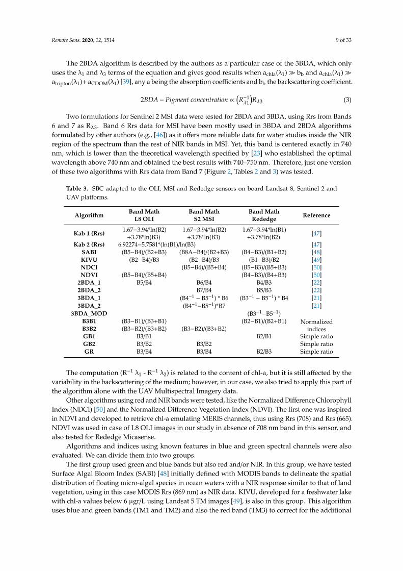
Two formulations for Sentinel 2 MSI data were tested for 2BDA and 3BDA, using Rrs from Bands6 and 7 as Rλ3. Band 6 Rrs data for MSI have been mostly used in 3BDA and 2BDA algorithmsformulated by other authors (e.g., [46]) as it offers more reliable data for water studies inside the NIRregion of the spectrum than the rest of NIR bands in MSI. Yet, this band is centered exactly in 740nm, which is lower than the theoretical wavelength specified by [23] who established the optimalwavelength above 740 nm and obtained the best results with 740–750 nm. Therefore, just one versionof these two algorithms with Rrs data from Band 7 (Figure 2, Tables 2 and 3) was tested.

Table 3. SBC adapted to the OLI, MSI and Rededge sensors on board Landsat 8, Sentinel 2 andUAV platforms.

Algorithm Band MathL8 OLI

Band MathS2 MSI

Band MathRededge Reference

Kab 1 (Rrs) 1.67−3.94*ln(B2)+3.78*ln(B3)

1.67−3.94*ln(B2)+3.78*ln(B3)

1.67−3.94*ln(B1)+3.78*ln(B2) [47]

Kab 2 (Rrs) 6.92274−5.7581*(ln(B1)/ln(B3) [47]SABI (B5−B4)/(B2+B3) (B8A−B4)/(B2+B3) (B4−B3)/(B1+B2) [48]KIVU (B2−B4)/B3 (B2−B4)/B3 (B1−B3)/B2 [49]NDCI (B5−B4)/(B5+B4) (B5−B3)/(B5+B3) [50]NDVI (B5−B4)/(B5+B4) (B4−B3)/(B4+B3) [50]

2BDA_1 B5/B4 B6/B4 B4/B3 [22]2BDA_2 B7/B4 B5/B3 [22]3BDA_1 (B4−1

− B5−1) * B6 (B3−1− B5−1) * B4 [21]

3BDA_2 (B4−1−B5−1)*B7 [21]

3BDA_MOD (B3−1−B5−1)

B3B1 (B3−B1)/(B3+B1) (B2−B1)/(B2+B1) NormalizedindicesB3B2 (B3−B2)/(B3+B2) (B3−B2)/(B3+B2)

GB1 B3/B1 B2/B1 Simple ratioGB2 B3/B2 B3/B2 Simple ratioGR B3/B4 B3/B4 B2/B3 Simple ratio

The computation (R−1 λ1 - R−1 λ2) is related to the content of chl-a, but it is still affected by thevariability in the backscattering of the medium; however, in our case, we also tried to apply this part ofthe algorithm alone with the UAV Multispectral Imagery data.

Other algorithms using red and NIR bands were tested, like the Normalized Difference ChlorophyllIndex (NDCI) [50] and the Normalized Difference Vegetation Index (NDVI). The first one was inspiredin NDVI and developed to retrieve chl-a emulating MERIS channels, thus using Rrs (708) and Rrs (665).NDVI was used in case of L8 OLI images in our study in absence of 708 nm band in this sensor, andalso tested for Rededge Micasense.

Algorithms and indices using known features in blue and green spectral channels were alsoevaluated. We can divide them into two groups.

The first group used green and blue bands but also red and/or NIR. In this group, we have testedSurface Algal Bloom Index (SABI) [48] initially defined with MODIS bands to delineate the spatialdistribution of floating micro-algal species in ocean waters with a NIR response similar to that of landvegetation, using in this case MODIS Rrs (869 nm) as NIR data. KIVU, developed for a freshwater lakewith chl-a values below 6 µgr/L using Landsat 5 TM images [49], is also in this group. This algorithmuses blue and green bands (TM1 and TM2) and also the red band (TM3) to correct for the additional

Remote Sens. 2020, 12, 1514 10 of 33

radiance caused by the scattering of non-organic suspended matter (see Table 3 for formulation andreferences).

In the last group, we tested Kab1 and Kab2, algorithms developed including blue and green bandsand originally formulated for coastal areas using Landsat 7 ETM+ bands. Finally, in this group, we alsotested simple ratios (GB1, GB2) and normalized indices (B3B1, B3B2) using only the green and bluebands available for each sensor.

Linear fits were adjusted both to chl-a data and Ln (chl-a) data, this approach also being tested byother authors to account for the non-normal distribution of the chl-a values [47,51].

The validation of the best performing models was done, only in case of satellite data, with imagesof the previous and next years (2016 and 2018). For both years, the validation was done with data inthe chl-a range of 1–40 µgr/L for which the models were calibrated. A range of 4.38–20.42 µgr/L wasused in case of Landsat 8 OLI, and 4.38–34.64 µgr/L in case of Sentinel 2 MSI.

The statistical metrics used for the validation exercise were: Root Mean Square Error (RMSE,Equation (4)), Normalized Root Mean Square Error (NRMSE, Equation (5)), Mean Absolute PercentageError (MAPE, Equation (6)) and bias (Equation (7)).

RMSE =

√1/n

∑n

i=1

(ypi − ymi

)2, (4)

NRMSE =RMSE

ymmax − ymmin, (5)

MAPE =1n

n∑i=1

∣∣∣ypi − ymi

∣∣∣ymi

(6)

bias =1n

n∑i=1

(ypi − ymi

), (7)

where yp is the predicted values, ym is the measured values and n is the number of samples.

3. Results

3.1. Water Quality

The studied reservoir is an eutrophic waterbody with recurrent cyanobacterial blooms since 2012,documented through the Galician Platform for Environmental Information (GAIA) (www.gaia.xunta.es)(Table 1). This periodic monitoring showed during 2017 Microcystis sp. as the dominant cyanobacteria,even though Chorococcus sp., Aphanocapsa sp. and Woronischia sp. were also present. The chl-a reacheda maximum in the BC point (which is considered more representative of the main waterbody) of21.26 µgr/L during May being the mean value for this year in BC sampling point 11.11 µgr/L. Thehighest cyanobacteria cell concentration was registered in October (9750 cel/mL) being Aphanocapsa sp.the dominant taxa. In the BP sampling point, the maximum chl-a was registered on 25th September(89.70 µgr/L), in this case, Microcystis sp. Being the dominant cyanobacterial taxa (115,500 cel/mL), andthe mean annual value 20.96 µgr/L [28]. During 2018 (when the second UAV flight was done) thegeneral condition of the reservoir was very different, with bigger cyanobacterial blooms, the mean andmaximum values of chl-a being higher than in 2017 (BCmean = 64.47 µgr/L, BPmean = 130.31 µgr/L).This documented highly changing condition in space and time makes this drinking water reservoir asuitable example of a sensible area which needs to be continuously monitored (Table 1).

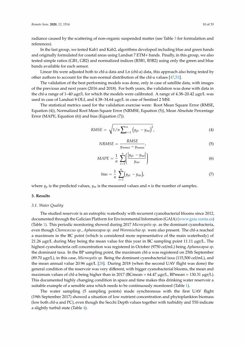
The water sampling (5 sampling points) made synchronous with the first UAV flight(19th September 2017) showed a situation of low nutrient concentration and phytoplankton biomass(low both chl-a and PC), even though the Secchi Depth values together with turbidity and TSS indicatea slightly turbid state (Table 4).

www.gaia.xunta.es

Remote Sens. 2020, 12, 1514 11 of 33

Table 4. Summary of the water analysis results of the in situ samplings synchronous with the UAVflights (DOC: Dissolved Organic Carbon; TSS: Total Suspended Solids; EC: Electrical Conductivity, Ptotal: Total Phosphorous).

2017 2018

Mean Max Min Mean Max Min

Chlorophyll a (µgr/L) 2.19 2.68 1.34 93.04 99.3 89.84Phycocyanin (µgr/L) 0.18 0.24 0.13 19.03 27.21 18.86

Turbidity (NTU) 4.16 5.20 3.07 2.3 2.8 1.4Sechi Disc Depth (m.) 1.7 2.0 1.5 1.6 1.75 1.20

pH Surface 7.18 7.26 7.04 7.22 7.32 7.08DOC (mg/L) 2.22 2.10 2.40 2.77 2.99 2.57TSS (mg/L) 3.20 6.8 1.2 21.5 27.2 18.0

OD sup (mg/L) 9.72 9.90 9.47 10.5 10.71 10.36Temp surface (◦C) 16.83 16.87 16.76 16.33 16.43 16.15EC surface (µS/cm) 129.6 131.0 128.0 127.0 127.0 127.0

P total (mg/L) 0.021 0.013Ammonium (mg/L) < 0.05

Nitrite (mg/L) 0.057Nitrate (mg/L) 9.27N total (mg/L) 2.20 2.76

Even though the phenological phase was considered the same in 2018 and in 2017, the secondUAV flight was done in very different water quality conditions with a cyanobacterial bloom in thereservoir and much higher chl-a and PC concentrations (Table 4). Curiously, turbidity was higher inthe first flight. Even though the same number of samples (5) was taken in either campaign, we have 4data in 2018 as one of the chl-a samples had to be discarded.

3.2. Spectral Band Combinations for the Retrieval of chl-a

The empirical approach was selected to build models for the retrieving of chl-a from the threetypes of multispectral images. All the indices and band ratios tested were adapted to the characteristicsof the bands of each sensor (Tables 2 and 3, Figure 2). In case of satellite imagery, the time windowused for the development of the algorithms (3 days) can be a source of error in case of sudden changesin the development of an algal bloom. The chosen year for the calibration of the models was the onewith more potential matchups (more in situ data) and stable conditions regarding chl-a concentration(cf. Table 1), in order to reduce the uncertainty in the calibration of the models regarding this timedifference. To evaluate this effect, we plotted the scatter plot graphics for the calibrated models forretrieving chl-a with a color code reflecting this time difference (0–3 days) (e.g., Figure 4F).

3.2.1. Landsat 8 Imagery

In the calibration to find a suitable linear model for the determination of chl-a (Equation (1)) withLandsat 8 OLI multispectral data, most of the algorithms and band indices tested were positive andsignificatively correlated (Pearson correlation) with chl-a concentration (Table 5). The linear fit wasmade with both chl-a data inside an interval of 5.65–18.09 µgr/L, and Ln transformed chl-a data, givingthe latter the best results.

Remote Sens. 2020, 12, 1514 12 of 33


and significatively correlated (Pearson correlation) with chl-a concentration (Table 5). The linear fit was made with both chl-a data inside an interval of 5.65 – 18.09 µgr/l, and Ln transformed chl-a data, giving the latter the best results.

Given the inherent complexity of inland waters, the combinations using red and NIR bands, specifically 2BDA, SABI and NDVI, were the best performing Spectral Band Combinations. The Surface Algal Bloom Index (SABI) which uses green and blue bands in addition to red and NIR [48] also gave good results. These three had the strongest (Pearson r > 0.8) and the more significative correlations with Ln(chl-a) data (Table 5, Figure 4). The results obtained with un-transformed Ln data did not show high differences, the Pearson r and R2 being 0.858 and 0.753 for 2BDA, 0.844 and 0.712 for SABI and 0.834 and 0.6953 for NDVI models, respectively. Kab_1 was also tested as its results were considered good, but the scatterplot showed a relationship based in two defined and separated group of points.

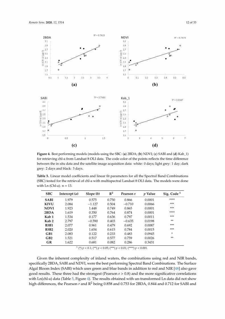
Table 5. Linear model coefficients and linear fit parameters for all the Spectral Band Combinations (SBC) tested for the retrieval of chl-a with multispectral Landsat 8 OLI data. The models were done with Ln (Chl-a). n = 13.

SBC Intercept (a) Slope (b) R2 Pearson r p Value Sig. Code(1) SABI 1.979 0.575 0.750 0.866 0.0001 **** KIVU 2.084 –1.127 0.504 –0.710 0.0066 *** NDVI 1.923 1.448 0.749 0.865 0.0001 *** 2BDA 1.619 0.350 0.764 0.874 0.0001 **** Kab 1 1.534 0.177 0.636 0.797 0.0011 *** Kab 2 2.797 –0.590 0.403 –0.635 0.0198 ** B3B1 2.077 0.961 0.479 0.692 0.0087 *** B3B2 2.020 1.654 0.615 0.784 0.0015 *** GB1 2.083 0.122 0.233 0.483 0.0945 * GB2 1.521 0.517 0.577 0.759 0.0026 ** GR 1.622 0.681 0.082 0.286 0.3431

1 (*) p<0.1; (**) p<0.05; (***) p<0.01; (****) p<0.001

(a)

(b)

(c)

(d)

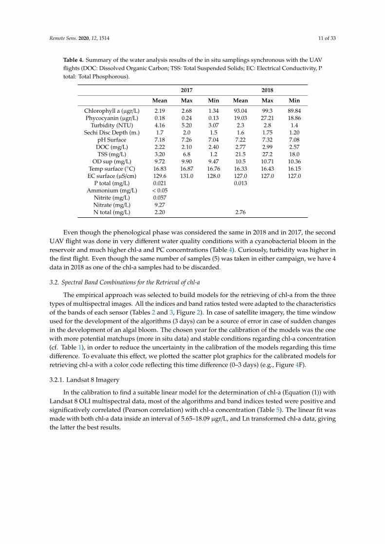
Figure 4. Best performing models (models using the SBC: (a) 2BDA; (b) NDVI; (c) SABI and (d) Kab_1)for retrieving chl-a from Landsat 8 OLI data. The code color of the points reflects the time differencebetween the in situ data and the satellite image acquisition data: white: 0 days; light grey: 1 day; darkgrey: 2 days and black: 3 days.

Table 5. Linear model coefficients and linear fit parameters for all the Spectral Band Combinations(SBC) tested for the retrieval of chl-a with multispectral Landsat 8 OLI data. The models were donewith Ln (Chl-a). n = 13.

SBC Intercept (a) Slope (b) R2 Pearson r p Value Sig. Code 1

SABI 1.979 0.575 0.750 0.866 0.0001 ****KIVU 2.084 −1.127 0.504 −0.710 0.0066 ***NDVI 1.923 1.448 0.749 0.865 0.0001 ***2BDA 1.619 0.350 0.764 0.874 0.0001 ****Kab 1 1.534 0.177 0.636 0.797 0.0011 ***Kab 2 2.797 −0.590 0.403 −0.635 0.0198 **B3B1 2.077 0.961 0.479 0.692 0.0087 ***B3B2 2.020 1.654 0.615 0.784 0.0015 ***GB1 2.083 0.122 0.233 0.483 0.0945 *GB2 1.521 0.517 0.577 0.759 0.0026 **GR 1.622 0.681 0.082 0.286 0.3431

1 (*) p < 0.1; (**) p < 0.05; (***) p < 0.01; (****) p < 0.001.

Given the inherent complexity of inland waters, the combinations using red and NIR bands,specifically 2BDA, SABI and NDVI, were the best performing Spectral Band Combinations. The SurfaceAlgal Bloom Index (SABI) which uses green and blue bands in addition to red and NIR [48] also gavegood results. These three had the strongest (Pearson r > 0.8) and the more significative correlationswith Ln(chl-a) data (Table 5, Figure 4). The results obtained with un-transformed Ln data did not showhigh differences, the Pearson r and R2 being 0.858 and 0.753 for 2BDA, 0.844 and 0.712 for SABI and

Remote Sens. 2020, 12, 1514 13 of 33

0.834 and 0.6953 for NDVI models, respectively. Kab_1 was also tested as its results were consideredgood, but the scatterplot showed a relationship based in two defined and separated group of points.

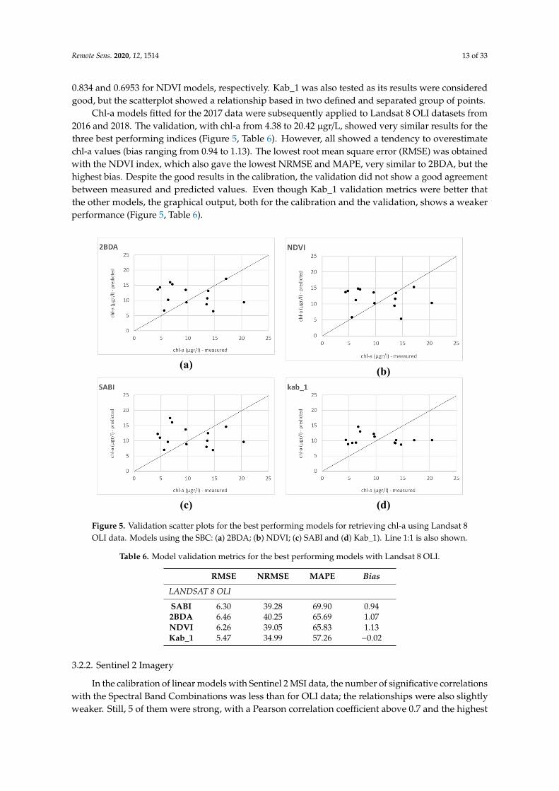
Chl-a models fitted for the 2017 data were subsequently applied to Landsat 8 OLI datasets from2016 and 2018. The validation, with chl-a from 4.38 to 20.42 µgr/L, showed very similar results for thethree best performing indices (Figure 5, Table 6). However, all showed a tendency to overestimatechl-a values (bias ranging from 0.94 to 1.13). The lowest root mean square error (RMSE) was obtainedwith the NDVI index, which also gave the lowest NRMSE and MAPE, very similar to 2BDA, but thehighest bias. Despite the good results in the calibration, the validation did not show a good agreementbetween measured and predicted values. Even though Kab_1 validation metrics were better thatthe other models, the graphical output, both for the calibration and the validation, shows a weakerperformance (Figure 5, Table 6).


Figure 4. Best performing models (models using the SBC: (a) 2BDA; (b) NDVI; (c) SABI and (d) Kab_1) for retrieving chl-a from Landsat 8 OLI data. The code color of the points reflects the time difference between the in situ data and the satellite image acquisition data: white: 0 days; light grey: 1 day; dark grey: 2 days and black: 3 days.

Chl-a models fitted for the 2017 data were subsequently applied to Landsat 8 OLI datasets from 2016 and 2018. The validation, with chl-a from 4.38 to 20.42 µgr/l, showed very similar results for the three best performing indices (Figure 5, Table 6). However, all showed a tendency to overestimate chl-a values (bias ranging from 0.94 to 1.13). The lowest root mean square error (RMSE) was obtained with the NDVI index, which also gave the lowest NRMSE and MAPE, very similar to 2BDA, but the highest bias. Despite the good results in the calibration, the validation did not show a good agreement between measured and predicted values. Even though Kab_1 validation metrics were better that the other models, the graphical output, both for the calibration and the validation, shows a weaker performance (Figure 5, Table 6).

(a)

(b)

(c)

(d)

Figure 5. Validation scatter plots for the best performing models for retrieving chl-a using Landsat 8 OLI data. Models using the SBC: (a) 2BDA; (b) NDVI; (c) SABI and (d) Kab_1). Line 1:1 is also shown.

Table 6. Model validation metrics for the best performing models with Landsat 8 OLI.

RMSE NRMSE MAPE Bias LANDSAT 8 OLI SABI 6.30 39.28 69.90 0.94 2BDA 6.46 40.25 65.69 1.07 NDVI 6.26 39.05 65.83 1.13 Kab_1 5.47 34.99 57,26 -0.02

3.2.2. Sentinel 2 Imagery

In the calibration of linear models with Sentinel 2 MSI data, the number of significative correlations with the Spectral Band Combinations was less than for OLI data; the relationships were also slightly weaker. Still, 5 of them were strong, with a Pearson correlation coefficient above 0.7 and

Figure 5. Validation scatter plots for the best performing models for retrieving chl-a using Landsat 8OLI data. Models using the SBC: (a) 2BDA; (b) NDVI; (c) SABI and (d) Kab_1). Line 1:1 is also shown.

Table 6. Model validation metrics for the best performing models with Landsat 8 OLI.

RMSE NRMSE MAPE Bias

LANDSAT 8 OLI

SABI 6.30 39.28 69.90 0.942BDA 6.46 40.25 65.69 1.07NDVI 6.26 39.05 65.83 1.13Kab_1 5.47 34.99 57.26 −0.02

3.2.2. Sentinel 2 Imagery

In the calibration of linear models with Sentinel 2 MSI data, the number of significative correlationswith the Spectral Band Combinations was less than for OLI data; the relationships were also slightlyweaker. Still, 5 of them were strong, with a Pearson correlation coefficient above 0.7 and the highest

Remote Sens. 2020, 12, 1514 14 of 33

significance level. In this case, the best fits were obtained with the chl-a value, and not with the Lntransformed data. The chl-a values in this case ranged from 5.09 to 50.37 µgr/L.

As with OLI data, all the linear models with Pearson r > 0.8 and a p value lower than 0.0001 wereconsidered the best performing and were tested in the validation stage. In this case, we also included inthe validation the 3BDA algorithm, as it also gave good results and the correlation coefficient was closeto 0.8 (Table 6). In case of Sentinel 2 data, not only did the combination of the NIR and red bands fitbest with chl-a values but also 3 Spectral Band Combinations with green and blue bands gave similarlygood results (Table 7, Figure 6).

Table 7. Linear model coefficients and linear fit parameters for all the Spectral Band Combinationstested for the retrieval of chl-a with multispectral Sentinel 2 MSI data. The models were done with insitu chl-a. n = 23.

Index Intercept (a) Slope (b) R2 Pearson r p Value Sig. Code 1

SABI 5.885 31.716 0.112 0.335 0.1274KIVU 24.360 −28.930 0.296 −0.544 0.0089 ***NDCI 10.130 61.300 0.213 0.461 0.0306 **

2BDA_1 29.516 −9.168 0.174 −0.417 0.0532 *2BDA_2 −30.740 22.850 0.702 0.837 0.0000 ****3BDA_1 14.515 3.597 0.006 0.081 0.72033BDA_2 7.134 26.795 0.532 0.729 0.0001 ****Kab_1 −5.064 6.361 0.679 0.824 0.0000 ****B3B2 8.662 61.763 0.673 0.820 0.0000 ****GB2 1.611 10.119 0.656 0.810 0.0000 ****GR 2.766 6.108 0.073 0.270 0.2234

1 (*) p < 0.1; (**) p < 0.05; (***) p < 0.01; (****) p < 0.001.


the highest significance level. In this case, the best fits were obtained with the chl-a value, and not with the Ln transformed data. The chl-a values in this case ranged from 5.09 to 50.37 µgr/l.

As with OLI data, all the linear models with Pearson r > 0.8 and a p value lower than 0.0001 were considered the best performing and were tested in the validation stage. In this case, we also included in the validation the 3BDA algorithm, as it also gave good results and the correlation coefficient was close to 0.8 (Table 6). In case of Sentinel 2 data, not only did the combination of the NIR and red bands fit best with chl-a values but also 3 Spectral Band Combinations with green and blue bands gave similarly good results (Table 7, Figure 6).

The results obtained in the linear fits with Ln transformed data showed a lower performance in case of Sentinel 2, the Pearson r and R2 being 0.718 and 0.5167 for 2BDA_2, 0.660 and 0.436 for 3BDA_2, 0.653 and 0.427 for Kab_1 and 0.659 and 0.435 for B3B2, respectively.

Table 7. Linear model coefficients and linear fit parameters for all the Spectral Band Combinations tested for the retrieval of chl-a with multispectral Sentinel 2 MSI data. The models were done with in situ chl-a. n=23.

Index Intercept (a) Slope (b) R2 Pearson r p Value Sig. Code(1) SABI 5.885 31.716 0.112 0.335 0.1274 KIVU 24.360 –28.930 0.296 –0.544 0.0089 *** NDCI 10.130 61.300 0.213 0.461 0.0306 ** 2BDA_1 29.516 –9.168 0.174 –0.417 0.0532 * 2BDA_2 –30.740 22.850 0.702 0.837 0.0000 **** 3BDA_1 14.515 3.597 0.006 0.081 0.7203 3BDA_2 7.134 26.795 0.532 0.729 0.0001 **** Kab_1 –5.064 6.361 0.679 0.824 0.0000 **** B3B2 8.662 61.763 0.673 0.820 0.0000 **** GB2 1.611 10.119 0.656 0.810 0.0000 **** GR 2.766 6.108 0.073 0.270 0.2234

1 (*) p<0.1; (**) p<0.05; (***) p<0.01; (****) p<0.001

(a)

(b)

(c)

(d)

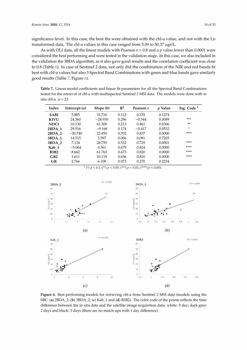
Figure 6. Best performing models for retrieving chl-a from Sentinel 2 MSI data (models using theSBC: (a) 2BDA_2; (b) 3BDA_2; (c) Kab_1 and (d) B3B2). The color code of the points reflects the timedifference between the in situ data and the satellite image acquisition data: white: 0 day; dark grey:2 days and black: 3 days (there are no match-ups with 1 day difference).

Remote Sens. 2020, 12, 1514 15 of 33

The results obtained in the linear fits with Ln transformed data showed a lower performance incase of Sentinel 2, the Pearson r and R2 being 0.718 and 0.5167 for 2BDA_2, 0.660 and 0.436 for 3BDA_2,0.653 and 0.427 for Kab_1 and 0.659 and 0.435 for B3B2, respectively.

As can be seen in Figure 6, the models using blue and green bands (Kab_1, B3B2) gave relativelyhigh R2 values but the correlation was highly dependent on one data point, so they were not consideredrobust. The results of the calibration/validation exercise are given (Table 8, Figure 7).

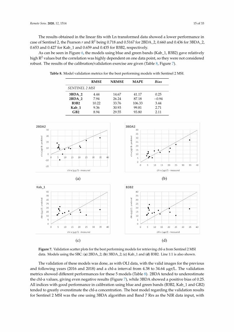
Table 8. Model validation metrics for the best performing models with Sentinel 2 MSI.

RMSE NRMSE MAPE Bias

SENTINEL 2 MSI

3BDA_2 4.44 14.67 41.17 0.252BDA_2 7.94 26.24 87.18 −0.94

B3B2 10.22 33.76 106.33 3.44Kab_1 9.36 30.93 99.81 2.71GB2 8.94 29.55 93.80 2.11


Figure 6. Best performing models for retrieving chl-a from Sentinel 2 MSI data (models using the SBC: (a) 2BDA_2; (b) 3BDA_2; (c) Kab_1 and (d) B3B2). The color code of the points reflects the time difference between the in situ data and the satellite image acquisition data: white: 0 day; dark grey: 2 days and black: 3 days (there are no match-ups with 1 day difference).

As can be seen in Figure 6, the models using blue and green bands (Kab_1, B3B2) gave relatively high R2 values but the correlation was highly dependent on one data point, so they were not considered robust. The results of the calibration/validation exercise are given (Table 8, Figure 7).

The validation of these models was done, as with OLI data, with the valid images for the previous and following years (2016 and 2018) and a chl-a interval from 4.38 to 34.64 µgr/l. The validation metrics showed different performances for these 5 models (Table 8). 2BDA tended to underestimate the chl-a values, giving even negative results (Figure 7), while 3BDA showed a positive bias of 0.25. All indices with good performance in calibration using blue and green bands (B3B2, Kab_1 and GB2) tended to greatly overestimate the chl-a concentration. The best model regarding the validation results for Sentinel 2 MSI was the one using 3BDA algorithm and Band 7 Rrs as the NIR data input, with the lowest values for all metrics, followed by 2BDA, as can also be seen in the validation scatterplots (Figure 7)

Table 8. Model validation metrics for the best performing models with Sentinel 2 MSI.

RMSE NRMSE MAPE Bias SENTINEL 2 MSI 3BDA_2 4.44 14.67 41.17 0.25 2BDA_2 7.94 26.24 87.18 -0.94

B3B2 10.22 33.76 106.33 3.44 Kab_1 9.36 30.93 99.81 2.71 GB2 8.94 29.55 93.80 2.11

(a)

(b)

(c)

(d)

Figure 7. Validation scatter plots for the best performing models for retrieving chl-a from Sentinel 2 MSIdata. Models using the SBC: (a) 2BDA_2; (b) 3BDA_2; (c) Kab_1 and (d) B3B2. Line 1:1 is also shown.

The validation of these models was done, as with OLI data, with the valid images for the previousand following years (2016 and 2018) and a chl-a interval from 4.38 to 34.64 µgr/L. The validationmetrics showed different performances for these 5 models (Table 8). 2BDA tended to underestimatethe chl-a values, giving even negative results (Figure 7), while 3BDA showed a positive bias of 0.25.All indices with good performance in calibration using blue and green bands (B3B2, Kab_1 and GB2)tended to greatly overestimate the chl-a concentration. The best model regarding the validation resultsfor Sentinel 2 MSI was the one using 3BDA algorithm and Band 7 Rrs as the NIR data input, with

Remote Sens. 2020, 12, 1514 16 of 33

the lowest values for all metrics, followed by 2BDA, as can also be seen in the validation scatterplots(Figure 7)

A clear pattern regarding the influence of the time window in the calibration of the algorithms(Figures 4 and 6) could not be found in the graphical analysis for Sentinel 2 but Landsat 8 graphicsshowed the worst fit for the 3-day time-lapse points. Overall, once the validation was done, thebest performing model for retrieving chl-a in the studied reservoir was the one fitted with the 3BDAalgorithm applied to Sentinel 2 imagery. The validation results for Landsat 8 were poorer thanSentinel 2.

3.2.3. UAV Imagery. Model Calibration

The two UAV flights (2017 and 2018) were made in late summer-early autumn, when thecyanobacterial bloom events take place in this area. This sampling plan was intended to calibrate andsubsequently validate the models; but two opposite conditions of algal bloom development were found(extremely different chl-a values, cf. Table 4). The chl-a interval covered was too broad to validate themodels obtained with the 2017 flight with the data of the 2018 flight, so the validation was not possible.Nevertheless, these two opposite situations gave the opportunity to test the multispectral sensorperformance in low and high chl-a concentrations, test the coherence of the relationships betweenflights and to test which of the Spectral Band Combinations were most “portable” to monitor chl-aconcentration in waterbodies with different eutrophication levels.

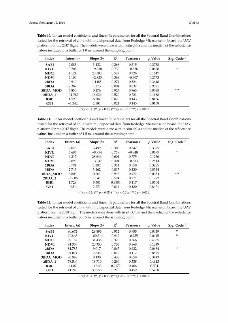
The 2017 flight, done in low chl-a concentration conditions, showed a better performance of theSpectral Band Combinations using NIR and red bands. Even though some positive correlations werefound, the only significative one applies a modified version of the 3BDA model (3BDA_MOD), for allthe three sampling areas tested. (Tables 9–11, Figure 8).

The second flight results, done in high chl-a concentration conditions, confirmed the combinationof red and NIR bands as the most suitable for chl-a retrieval with the Rededge Micasense sensor. Inthis case, the best performing models were always 2BDA and SABI (Figure 8, Tables 12–14).

In another exercise, the data of both flights were analyzed together. We used the 9 available points(5 from 2017 and 4 for 2018) to calibrate linear models that could be adjusted to this broad range of chl-aconcentrations. As it was assessed that the results were similar for the 3 buffers tested (Tables 9–14),this exercise was done only with the 0.5-m. buffer data. Even though this uneven distribution of data isassociated with a high level of uncertainty, we considered the obtained results promising and worthyof being shown.

Table 9. Linear model coefficients and linear fit parameters for all the Spectral Band Combinationstested for the retrieval of chl-a with multispectral data from Rededge Micasense on board the UAVplatform for the 2017 flight. The models were done with in situ chl-a and the median of the reflectancevalues included in a buffer of 0.5 m. around the sampling point.

Index Interc. (a) Slope (b) R2 Pearson r p Value Sig. Code 1

SABI 2.073 3.085 0.264 0.514 0.3755KIVU 3.665 −9.405 0.711 −0.843 0.0727 *NDCI 4.091 28.404 0.603 0.776 0.1225NDVI 2.088 2.778 0.363 0.603 0.28192BDA 0.970 1.109 0.267 0.517 0.37213BDA 3.262 7.039 0.046 0.215 0.7279

3BDA_MOD 3.715 0.2615 0.945 0.972 0.0055 ***2BDA_2 −12.031 16.256 0.597 0.773 0.1256

B3B1 1.371 9.470 0.037 0.193 0.7549GB1 −2.578 4.008 0.038 0.195 0.7526

1 (*) p < 0.1(**) p < 0.05; (***) p < 0.01; (****) p < 0.001.

Remote Sens. 2020, 12, 1514 17 of 33


Index Interc (a) Slope (b) R2 Pearson r p Value Sig. Code 1

SABI 2.083 3.132 0.266 0.515 0.3738KIVU 3.708 −9.950 0.733 −0.856 0.0638 *NDCI 4.124 28.100 0.527 0.726 0.1647NDVI 2.100 −2.823 0.369 −0.607 0.27732BDA 0.940 1.1485 0.274 0.524 0.36483BDA 2.387 1.273 0.001 0.037 0.9521

3BDA_MOD 3.830 0.276 0.927 0.963 0.0085 ***2BDA_2 −11.787 16.039 0.520 0.721 0.1688

B3B1 1.599 6.787 0.020 0.143 0.8186GB1 −1.242 2.881 0.021 0.145 0.8158

1 (*) p < 0.1; (**) p < 0.05; (***) p < 0.01; (****) p < 0.001.



SABI 2.078 3.499 0.300 0.547 0.3395KIVU 3.696 −9.954 0.719 −0.848 0.0695 *NDCI 4.217 28.646 0.601 0.775 0.1236NDVI 2.099 −3.047 0.401 −0.633 0.25142BDA 0.791 1.292 0.311 0.558 0.32853BDA 2.743 3.462 0.017 0.130 0.8344

3BDA_MOD 3.803 0.264 0.946 0.972 0.0054 ***2BDA_2 −12.06 16.41 0.594 0.771 0.1272

B3B1 1.729 5.301 0.8504 0.117 0.8504GB1 −0.514 2.271 0.014 0.120 0.8471

1 (*) p < 0.1; (**) p < 0.05; (***) p < 0.01; (****) p < 0.001.

Table 12. Linear model coefficients and linear fit parameters for all the Spectral Band Combinationstested for the retrieval of chl-a with multispectral data from Rededge Micasense on board the UAVplatform for the 2018 flight. The models were done with in situ Chl-a and the median of the reflectancevalues included in a buffer of 0.5 m. around the sampling point.


SABI 90.672 28.895 0.912 0.955 0.0449 **KIVU 102.65 −80.314 0.912 −0.955 0.0445 **NDCI 97.157 31.436 0.320 0.566 0.4335NDVI 91.359 20.330 0.753 0.868 0.13192BDA 81.783 9.017 0.867 0.932 0.0684 *3BDA 94.014 2.844 0.012 0.112 0.8875

3BDA_MOD 96.948 0.130 0.433 0.658 0.34132BDA_2 78.540 18.710 0.290 0.538 0.4613

B3B1 64.07 112.43 0.2172 0.466 0.534GB1 41.240 30.550 0.210 0.459 0.5408

1 (*) p < 0.1; (**) p < 0.05; (***) p < 0.01; (****) p < 0.001.

Remote Sens. 2020, 12, 1514 18 of 33



SABI 90.684 29.020 0.911 0.9542 0.0457 **KIVU 102.671 −80.930 0.907 −0.952 0.0477 **NDCI 96.906 29.599 0.288 0.536 0.4634NDVI 91.375 20.373 0.752 0.867 0.13302BDA 81.747 9.068 0.865 0.930 0.0696 *3BDA 93.583 1.587 0.004 0.064 0.9358

3BDA_MOD 93.837 0.127 0.410 0.640 0.35912BDA_2 79.550 17.390 0.256 0.506 0.4937

B3B1 68.00 97.26 0.1573 0.396 0.6033GB1 48.590 26.230 0.151 0.388 0.6114

1 (*) p < 0.1; (**) p < 0.05; (***) p < 0.01; (****) p < 0.001.



SABI 90.672 29.021 0.9099 0.9539 0.0461 **KIVU 102.730 −81.120 0.9056 0.9516 0.0483 **NDCI 97.096 31.118 0.308 0.5550 0.4450NDVI 91.361 20.354 0.750 0.8660 0.13402BDA 81.740 9.060 0.8651 0.9301 0.0698 *3BDA 93.810 2.270 0.0079 0.0891 0.9109

3BDA_MOD 96.936 0.1305 0.4257 0.6524 0.34752BDA_2 78.740 18.430 0.2772 0.5265 0.4735

B3B1 66.56 102.88 0.1709 0.4133 0.5867GB1 45.950 27.790 0.1644 0.4054 0.5945

1 (*) p < 0.1; (**) p < 0.05; (***) p < 0.01; (****) p < 0.001.

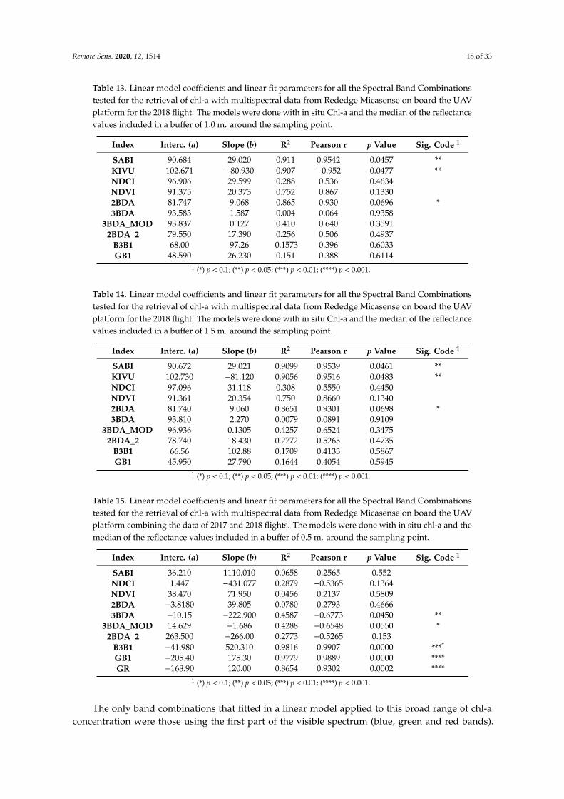
Table 15. Linear model coefficients and linear fit parameters for all the Spectral Band Combinationstested for the retrieval of chl-a with multispectral data from Rededge Micasense on board the UAVplatform combining the data of 2017 and 2018 flights. The models were done with in situ chl-a and themedian of the reflectance values included in a buffer of 0.5 m. around the sampling point.


SABI 36.210 1110.010 0.0658 0.2565 0.552NDCI 1.447 −431.077 0.2879 −0.5365 0.1364NDVI 38.470 71.950 0.0456 0.2137 0.58092BDA −3.8180 39.805 0.0780 0.2793 0.46663BDA −10.15 −222.900 0.4587 −0.6773 0.0450 **

3BDA_MOD 14.629 −1.686 0.4288 −0.6548 0.0550 *2BDA_2 263.500 −266.00 0.2773 −0.5265 0.153

B3B1 −41.980 520.310 0.9816 0.9907 0.0000 ****

GB1 −205.40 175.30 0.9779 0.9889 0.0000 ****GR −168.90 120.00 0.8654 0.9302 0.0002 ****

1 (*) p < 0.1; (**) p < 0.05; (***) p < 0.01; (****) p < 0.001.

The only band combinations that fitted in a linear model applied to this broad range of chl-aconcentration were those using the first part of the visible spectrum (blue, green and red bands).

Remote Sens. 2020, 12, 1514 19 of 33

The combination of these bands (blue-green and green-red) gave the results shown in Table 15 andFigure 9. It can be seen that this relationship is based upon two separate groups of points, so it is notconsidered good for directly retrieving absolute chl-a values accurately; however, the results suggestedthat it can be used to classify the pixels into broad chl-a categories or classes to which apply algorithmsspecific to this narrower chl-a range inside of each class. This is also a key issue when dealing withcyanobacterial blooms with a spatial patchy distribution in waterbodies, in order to spatially stratifythe analyses.


SABI 90.684 29.020 0.911 0.9542 0.0457 ** KIVU 102.671 –80.930 0.907 -0.952 0.0477 ** NDCI 96.906 29.599 0.288 0.536 0.4634 NDVI 91.375 20.373 0.752 0.867 0.1330 2BDA 81.747 9.068 0.865 0.930 0.0696 * 3BDA 93.583 1.587 0.004 0.064 0.9358 3BDA_MOD 93.837 0.127 0.410 0.640 0.3591 2BDA_2 79.550 17.390 0.256 0.506 0.4937 B3B1 68.00 97.26 0.1573 0.396 0.6033 GB1 48.590 26.230 0.151 0.388 0.6114

1 (*) p<0.1; (**) p<0.05; (***) p<0.01; (****) p<0.001

Table 14. Linear model coefficients and linear fit parameters for all the Spectral Band Combinations tested for the retrieval of chl-a with multispectral data from Rededge Micasense on board the UAV platform for the 2018 flight. The models were done with in situ Chl-a and the median of the reflectance values included in a buffer of 1.5 m. around the sampling point.

Index Interc. (a) Slope (b) R2 Pearson r p Value Sig. Code(1) SABI 90.672 29.021 0.9099 0.9539 0.0461 ** KIVU 102.730 –81.120 0.9056 0.9516 0.0483 ** NDCI 97.096 31.118 0.308 0.5550 0.4450 NDVI 91.361 20.354 0.750 0.8660 0.1340 2BDA 81.740 9.060 0.8651 0.9301 0.0698 * 3BDA 93.810 2.270 0.0079 0.0891 0.9109

3BDA_MOD 96.936 0.1305 0.4257 0.6524 0.3475 2BDA_2 78.740 18.430 0.2772 0.5265 0.4735

B3B1 66.56 102.88 0.1709 0.4133 0.5867 GB1 45.950 27.790 0.1644 0.4054 0.5945

1 (*) p<0.1; (**) p<0.05; (***) p<0.01; (****) p<0.001

(a)

(b)

(c)

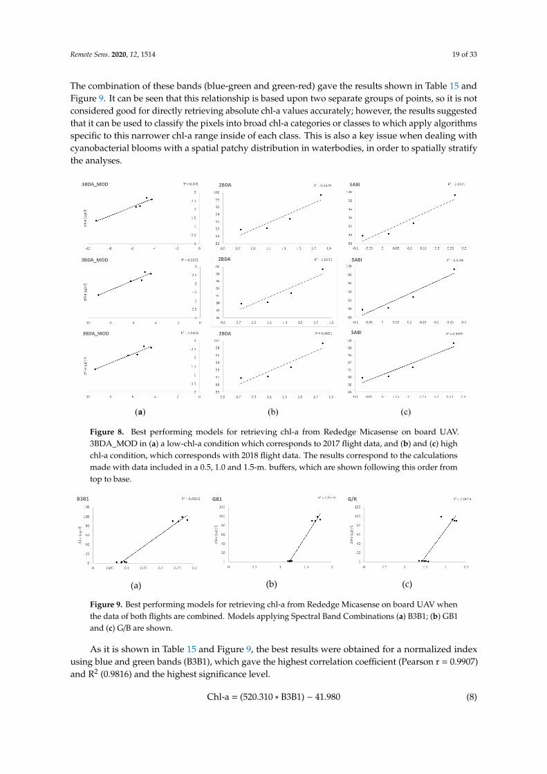
Figure 8. Best performing models for retrieving chl-a from Rededge Micasense on board UAV. 3BDA_MOD in (a) a low-chl-a condition which corresponds to 2017 flight data, and (b) and (c) high

Figure 8. Best performing models for retrieving chl-a from Rededge Micasense on board UAV.3BDA_MOD in (a) a low-chl-a condition which corresponds to 2017 flight data, and (b) and (c) highchl-a condition, which corresponds with 2018 flight data. The results correspond to the calculationsmade with data included in a 0.5, 1.0 and 1.5-m. buffers, which are shown following this order fromtop to base.


chl-a condition, which corresponds with 2018 flight data. The results correspond to the calculations made with data included in a 0.5, 1.0 and 1.5-m. buffers, which are shown following this order from top to base.

In another exercise, the data of both flights were analyzed together. We used the 9 available points (5 from 2017 and 4 for 2018) to calibrate linear models that could be adjusted to this broad range of chl-a concentrations. As it was assessed that the results were similar for the 3 buffers tested (Tables 9–14), this exercise was done only with the 0.5-m. buffer data. Even though this uneven distribution of data is associated with a high level of uncertainty, we considered the obtained results promising and worthy of being shown.

The only band combinations that fitted in a linear model applied to this broad range of chl-a concentration were those using the first part of the visible spectrum (blue, green and red bands). The combination of these bands (blue-green and green-red) gave the results shown in Table 15 and Figure 9. It can be seen that this relationship is based upon two separate groups of points, so it is not considered good for directly retrieving absolute chl-a values accurately; however, the results suggested that it can be used to classify the pixels into broad chl-a categories or classes to which apply algorithms specific to this narrower chl-a range inside of each class. This is also a key issue when dealing with cyanobacterial blooms with a spatial patchy distribution in waterbodies, in order to spatially stratify the analyses.

Table 15. Linear model coefficients and linear fit parameters for all the Spectral Band Combinations tested for the retrieval of chl-a with multispectral data from Rededge Micasense on board the UAV platform combining the data of 2017 and 2018 flights. The models were done with in situ chl-a and the median of the reflectance values included in a buffer of 0.5 m. around the sampling point.

Index Interc. (a) Slope (b) R2 Pearson r p Value Sig. Code(1)

SABI 36.210 1110.010 0.0658 0.2565 0.552 NDCI 1.447 –431.077 0.2879 –0.5365 0.1364 NDVI 38.470 71.950 0.0456 0.2137 0.5809 2BDA –3.8180 39.805 0.0780 0.2793 0.4666 3BDA –10.15 –222.900 0.4587 –0.6773 0.0450 ** 3BDA_MOD 14.629 –1.686 0.4288 –0.6548 0.0550 * 2BDA_2 263.500 –266.00 0.2773 –0.5265 0.153 B3B1 –41.980 520.310 0.9816 0.9907 0.0000 ****

GB1 –205.40 175.30 0.9779 0.9889 0.0000 **** GR –168.90 120.00 0.8654 0.9302 0.0002 ****

1 (*) p<0.1; (**) p<0.05; (***) p<0.01; (****) p<0.001

(a)

(b)

(c)

Figure 9. Best performing models for retrieving chl-a from Rededge Micasense on board UAV when the data of both flights are combined. Models applying Spectral Band Combinations (a) B3B1; (b) GB1 and (c) G/B are shown.

Figure 9. Best performing models for retrieving chl-a from Rededge Micasense on board UAV whenthe data of both flights are combined. Models applying Spectral Band Combinations (a) B3B1; (b) GB1and (c) G/B are shown.

As it is shown in Table 15 and Figure 9, the best results were obtained for a normalized indexusing blue and green bands (B3B1), which gave the highest correlation coefficient (Pearson r = 0.9907)and R2 (0.9816) and the highest significance level.

Chl-a = (520.310 ∗ B3B1) − 41.980 (8)

Remote Sens. 2020, 12, 1514 20 of 33

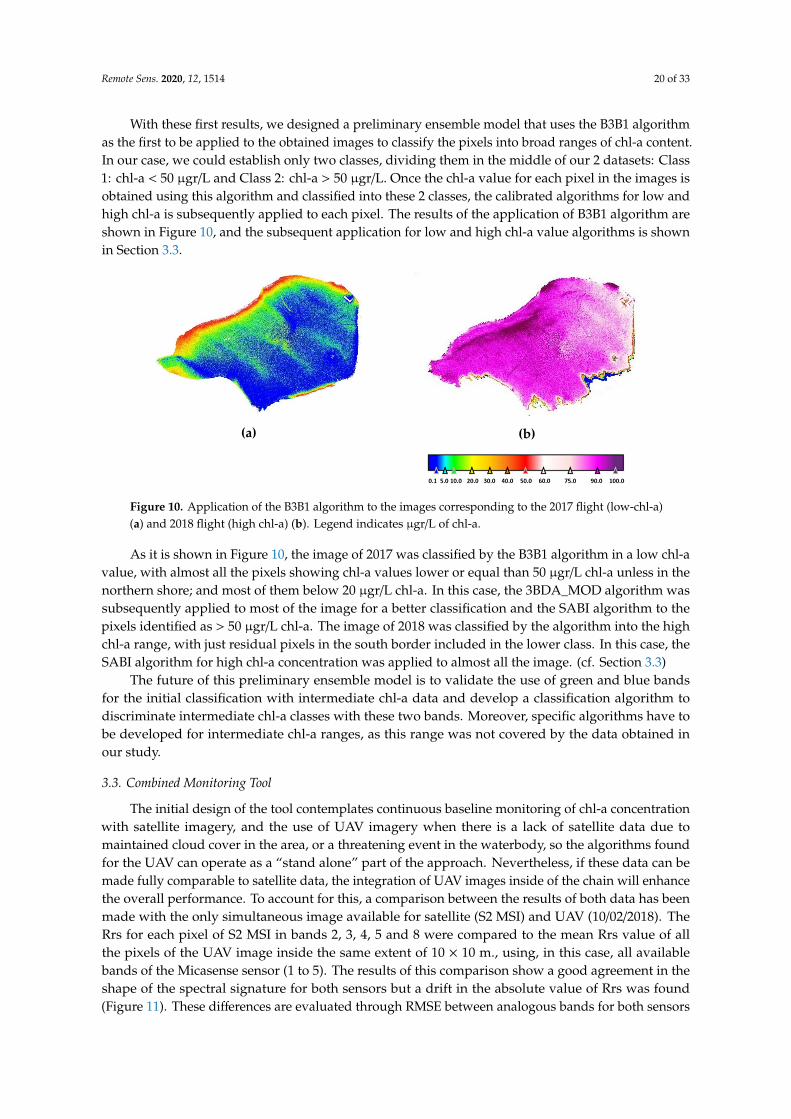
With these first results, we designed a preliminary ensemble model that uses the B3B1 algorithmas the first to be applied to the obtained images to classify the pixels into broad ranges of chl-a content.In our case, we could establish only two classes, dividing them in the middle of our 2 datasets: Class1: chl-a < 50 µgr/L and Class 2: chl-a > 50 µgr/L. Once the chl-a value for each pixel in the images isobtained using this algorithm and classified into these 2 classes, the calibrated algorithms for low andhigh chl-a is subsequently applied to each pixel. The results of the application of B3B1 algorithm areshown in Figure 10, and the subsequent application for low and high chl-a value algorithms is shownin Section 3.3.


As it is shown in Table 15 and Figure 9, the best results were obtained for a normalized index using blue and green bands (B3B1), which gave the highest correlation coefficient (Pearson r = 0.9907) and R2 (0.9816) and the highest significance level.

Chl-a = (520.310 * B3B1) – 41.980 (8)

With these first results, we designed a preliminary ensemble model that uses the B3B1 algorithm as the first to be applied to the obtained images to classify the pixels into broad ranges of chl-a content. In our case, we could establish only two classes, dividing them in the middle of our 2 datasets: Class 1: chl-a < 50 μgr/l and Class 2: chl-a > 50 μgr/l. Once the chl-a value for each pixel in the images is obtained using this algorithm and classified into these 2 classes, the calibrated algorithms for low and high chl-a is subsequently applied to each pixel. The results of the application of B3B1 algorithm are shown in Figure 10, and the subsequent application for low and high chl-a value algorithms is shown in section 3.3.

(a)

(b)

Figure 10. Application of the B3B1 algorithm to the images corresponding to the 2017 flight (low-chl-a) (a) and 2018 flight (high chl-a) (b). Legend indicates µgr/l of chl-a.

As it is shown in Figure 10, the image of 2017 was classified by the B3B1 algorithm in a low chl-a value, with almost all the pixels showing chl-a values lower or equal than 50 μgr/l chl-a unless in the northern shore; and most of them below 20 μgr/l chl-a. In this case, the 3BDA_MOD algorithm was subsequently applied to most of the image for a better classification and the SABI algorithm to the pixels identified as > 50 μgr/l chl-a. The image of 2018 was classified by the algorithm into the high chl-a range, with just residual pixels in the south border included in the lower class. In this case, the SABI algorithm for high chl-a concentration was applied to almost all the image. (cf. section 3.3)

The future of this preliminary ensemble model is to validate the use of green and blue bands for the initial classification with intermediate chl-a data and develop a classification algorithm to discriminate intermediate chl-a classes with these two bands. Moreover, specific algorithms have to be developed for intermediate chl-a ranges, as this range was not covered by the data obtained in our study.

3.3.Combined Monitoring Tool

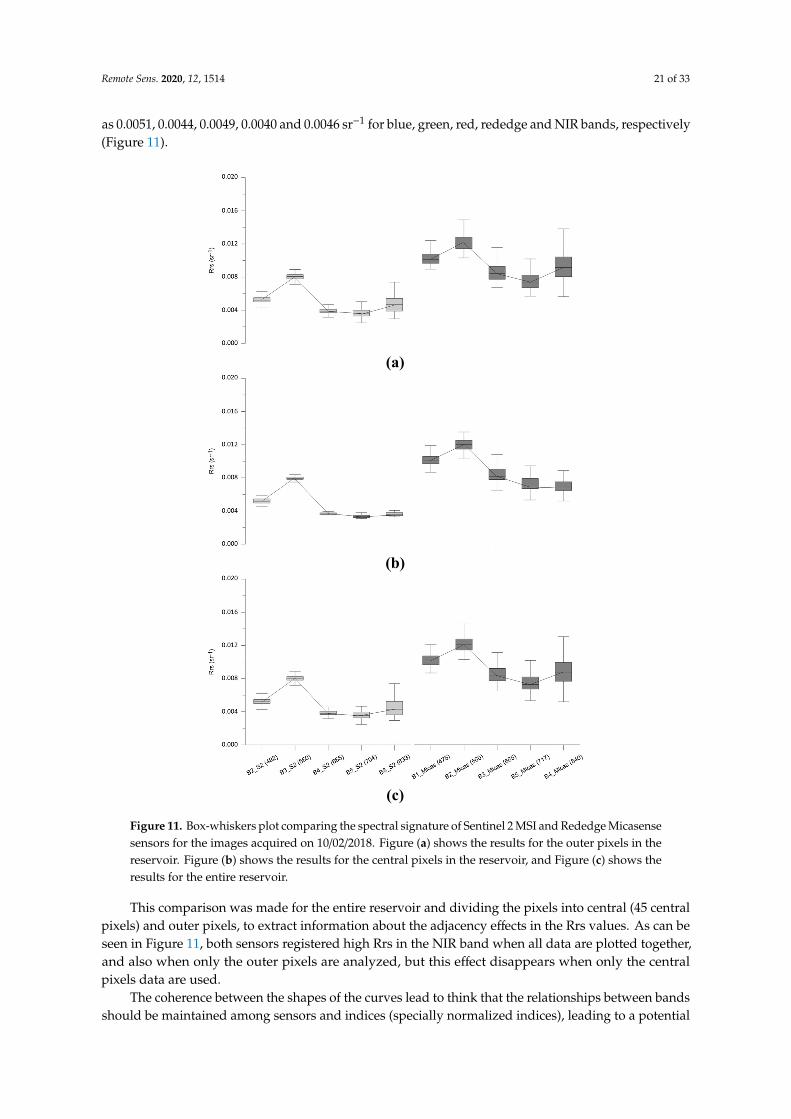
The initial design of the tool contemplates continuous baseline monitoring of chl-a concentration with satellite imagery, and the use of UAV imagery when there is a lack of satellite data due to maintained cloud cover in the area, or a threatening event in the waterbody, so the algorithms found for the UAV can operate as a “stand alone” part of the approach. Nevertheless, if these data can be made fully comparable to satellite data, the integration of UAV images inside of the chain will enhance the overall performance. To account for this, a comparison between the results of both data has been made with the only simultaneous image available for satellite (S2 MSI) and UAV (10/02/2018). The Rrs for each pixel of S2 MSI in bands 2, 3, 4, 5 and 8 were compared to the mean Rrs value of all the pixels of the UAV image inside the same extent of 10 × 10 m., using, in this case, all

Figure 10. Application of the B3B1 algorithm to the images corresponding to the 2017 flight (low-chl-a)(a) and 2018 flight (high chl-a) (b). Legend indicates µgr/L of chl-a.

As it is shown in Figure 10, the image of 2017 was classified by the B3B1 algorithm in a low chl-avalue, with almost all the pixels showing chl-a values lower or equal than 50 µgr/L chl-a unless in thenorthern shore; and most of them below 20 µgr/L chl-a. In this case, the 3BDA_MOD algorithm wassubsequently applied to most of the image for a better classification and the SABI algorithm to thepixels identified as > 50 µgr/L chl-a. The image of 2018 was classified by the algorithm into the highchl-a range, with just residual pixels in the south border included in the lower class. In this case, theSABI algorithm for high chl-a concentration was applied to almost all the image. (cf. Section 3.3)

The future of this preliminary ensemble model is to validate the use of green and blue bandsfor the initial classification with intermediate chl-a data and develop a classification algorithm todiscriminate intermediate chl-a classes with these two bands. Moreover, specific algorithms have tobe developed for intermediate chl-a ranges, as this range was not covered by the data obtained inour study.

3.3. Combined Monitoring Tool

The initial design of the tool contemplates continuous baseline monitoring of chl-a concentrationwith satellite imagery, and the use of UAV imagery when there is a lack of satellite data due tomaintained cloud cover in the area, or a threatening event in the waterbody, so the algorithms foundfor the UAV can operate as a “stand alone” part of the approach. Nevertheless, if these data can bemade fully comparable to satellite data, the integration of UAV images inside of the chain will enhancethe overall performance. To account for this, a comparison between the results of both data has beenmade with the only simultaneous image available for satellite (S2 MSI) and UAV (10/02/2018). TheRrs for each pixel of S2 MSI in bands 2, 3, 4, 5 and 8 were compared to the mean Rrs value of allthe pixels of the UAV image inside the same extent of 10 × 10 m., using, in this case, all availablebands of the Micasense sensor (1 to 5). The results of this comparison show a good agreement in theshape of the spectral signature for both sensors but a drift in the absolute value of Rrs was found(Figure 11). These differences are evaluated through RMSE between analogous bands for both sensors

Remote Sens. 2020, 12, 1514 21 of 33

as 0.0051, 0.0044, 0.0049, 0.0040 and 0.0046 sr−1 for blue, green, red, rededge and NIR bands, respectively(Figure 11).


available bands of the Micasense sensor (1 to 5). The results of this comparison show a good agreement in the shape of the spectral signature for both sensors but a drift in the absolute value of Rrs was found (Figure 11). These differences are evaluated through RMSE between analogous bands for both sensors as 0.0051, 0.0044, 0.0049, 0.0040 and 0.0046 sr-1 for blue, green, red, rededge and NIR bands, respectively (Figure 11).

(a)

(b)

(c)

Figure 11. Box-whiskers plot comparing the spectral signature of Sentinel 2 MSI and Rededge Micasense sensors for the images acquired on 10/02/2018. Figure (a) shows the results for the outer pixels in the reservoir. Figure (b) shows the results for the central pixels in the reservoir, and Figure (c) shows the results for the entire reservoir.

This comparison was made for the entire reservoir and dividing the pixels into central (45 central pixels) and outer pixels, to extract information about the adjacency effects in the Rrs values. As can be seen in Figure 11, both sensors registered high Rrs in the NIR band when all data are plotted together, and also when only the outer pixels are analyzed, but this effect disappears when only the central pixels data are used.

Figure 11. Box-whiskers plot comparing the spectral signature of Sentinel 2 MSI and Rededge Micasensesensors for the images acquired on 10/02/2018. Figure (a) shows the results for the outer pixels in thereservoir. Figure (b) shows the results for the central pixels in the reservoir, and Figure (c) shows theresults for the entire reservoir.

This comparison was made for the entire reservoir and dividing the pixels into central (45 centralpixels) and outer pixels, to extract information about the adjacency effects in the Rrs values. As can beseen in Figure 11, both sensors registered high Rrs in the NIR band when all data are plotted together,and also when only the outer pixels are analyzed, but this effect disappears when only the centralpixels data are used.

The coherence between the shapes of the curves lead to think that the relationships between bandsshould be maintained among sensors and indices (specially normalized indices), leading to a potential

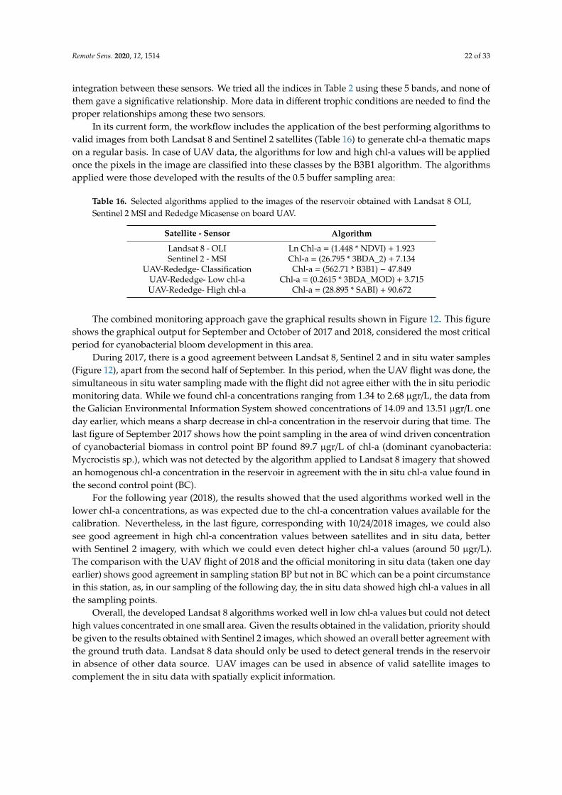
Remote Sens. 2020, 12, 1514 22 of 33

integration between these sensors. We tried all the indices in Table 2 using these 5 bands, and none ofthem gave a significative relationship. More data in different trophic conditions are needed to find theproper relationships among these two sensors.

In its current form, the workflow includes the application of the best performing algorithms tovalid images from both Landsat 8 and Sentinel 2 satellites (Table 16) to generate chl-a thematic mapson a regular basis. In case of UAV data, the algorithms for low and high chl-a values will be appliedonce the pixels in the image are classified into these classes by the B3B1 algorithm. The algorithmsapplied were those developed with the results of the 0.5 buffer sampling area:

Table 16. Selected algorithms applied to the images of the reservoir obtained with Landsat 8 OLI,Sentinel 2 MSI and Rededge Micasense on board UAV.

Satellite - Sensor Algorithm

Landsat 8 - OLI Ln Chl-a = (1.448 * NDVI) + 1.923Sentinel 2 - MSI Chl-a = (26.795 * 3BDA_2) + 7.134

UAV-Rededge- Classification Chl-a = (562.71 * B3B1) − 47.849UAV-Rededge- Low chl-a Chl-a = (0.2615 * 3BDA_MOD) + 3.715UAV-Rededge- High chl-a Chl-a = (28.895 * SABI) + 90.672

The combined monitoring approach gave the graphical results shown in Figure 12. This figureshows the graphical output for September and October of 2017 and 2018, considered the most criticalperiod for cyanobacterial bloom development in this area.

During 2017, there is a good agreement between Landsat 8, Sentinel 2 and in situ water samples(Figure 12), apart from the second half of September. In this period, when the UAV flight was done, thesimultaneous in situ water sampling made with the flight did not agree either with the in situ periodicmonitoring data. While we found chl-a concentrations ranging from 1.34 to 2.68 µgr/L, the data fromthe Galician Environmental Information System showed concentrations of 14.09 and 13.51 µgr/L oneday earlier, which means a sharp decrease in chl-a concentration in the reservoir during that time. Thelast figure of September 2017 shows how the point sampling in the area of wind driven concentrationof cyanobacterial biomass in control point BP found 89.7 µgr/L of chl-a (dominant cyanobacteria:Mycrocistis sp.), which was not detected by the algorithm applied to Landsat 8 imagery that showedan homogenous chl-a concentration in the reservoir in agreement with the in situ chl-a value found inthe second control point (BC).

For the following year (2018), the results showed that the used algorithms worked well in thelower chl-a concentrations, as was expected due to the chl-a concentration values available for thecalibration. Nevertheless, in the last figure, corresponding with 10/24/2018 images, we could alsosee good agreement in high chl-a concentration values between satellites and in situ data, betterwith Sentinel 2 imagery, with which we could even detect higher chl-a values (around 50 µgr/L).The comparison with the UAV flight of 2018 and the official monitoring in situ data (taken one dayearlier) shows good agreement in sampling station BP but not in BC which can be a point circumstancein this station, as, in our sampling of the following day, the in situ data showed high chl-a values in allthe sampling points.

Overall, the developed Landsat 8 algorithms worked well in low chl-a values but could not detecthigh values concentrated in one small area. Given the results obtained in the validation, priority shouldbe given to the results obtained with Sentinel 2 images, which showed an overall better agreement withthe ground truth data. Landsat 8 data should only be used to detect general trends in the reservoirin absence of other data source. UAV images can be used in absence of valid satellite images tocomplement the in situ data with spatially explicit information.

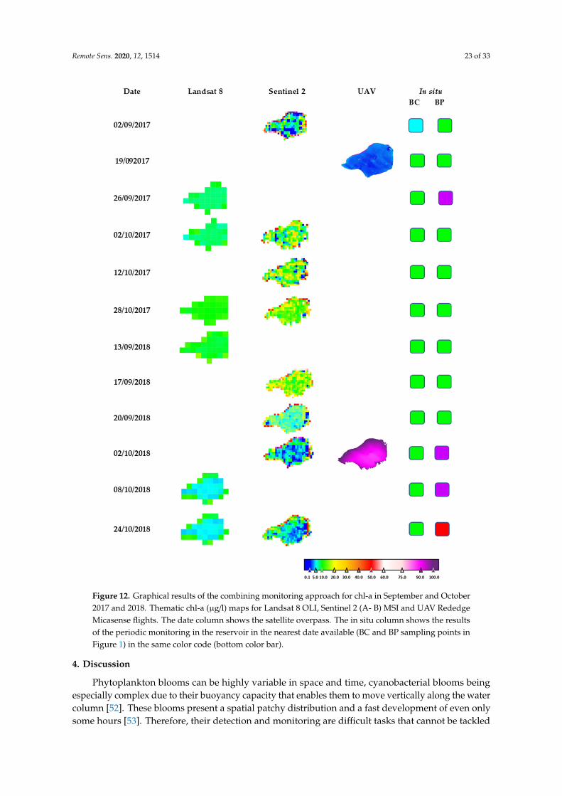
Remote Sens. 2020, 12, 1514 23 of 33


Figure 12. Graphical results of the combining monitoring approach for chl-a in September and October 2017 and 2018. Thematic chl-a (µg/l) maps for Landsat 8 OLI, Sentinel 2 (A- B) MSI and UAV Rededge Micasense flights. The date column shows the satellite overpass. The in situ column shows the results of the periodic monitoring in the reservoir in the nearest date available (BC and BP sampling points in Figure 1) in the same color code (bottom color bar).

During 2017, there is a good agreement between Landsat 8, Sentinel 2 and in situ water samples (Figure 12), apart from the second half of September. In this period, when the UAV flight was done, the simultaneous in situ water sampling made with the flight did not agree either with the in situ periodic monitoring data. While we found chl-a concentrations ranging from 1.34 to 2.68 µgr/l, the data from the Galician Environmental Information System showed concentrations of 14.09 and 13.51 µgr/l one day earlier, which means a sharp decrease in chl-a concentration in the reservoir during

Figure 12. Graphical results of the combining monitoring approach for chl-a in September and October2017 and 2018. Thematic chl-a (µg/l) maps for Landsat 8 OLI, Sentinel 2 (A- B) MSI and UAV RededgeMicasense flights. The date column shows the satellite overpass. The in situ column shows the resultsof the periodic monitoring in the reservoir in the nearest date available (BC and BP sampling points inFigure 1) in the same color code (bottom color bar).

4. Discussion

Phytoplankton blooms can be highly variable in space and time, cyanobacterial blooms beingespecially complex due to their buoyancy capacity that enables them to move vertically along the watercolumn [52]. These blooms present a spatial patchy distribution and a fast development of even onlysome hours [53]. Therefore, their detection and monitoring are difficult tasks that cannot be tackled

Remote Sens. 2020, 12, 1514 24 of 33

only by in situ point measurements; the synoptic view offered by satellites and UAV multispectral orhyperspectral imagery is an excellent complement to this routine type of sampling [14,54]

The data provided by Sentinel 2 and Landsat 8, when combined in the form of a virtual constellation,opened up new opportunities for capturing limnological dynamics that reflect rates of change at anunprecedent resolution [26,36,54]. The Landsat 8 equatorial repeat cycle (since 2013) is 16 days, whileeach of the Sentinels 2 is 10 days, which becomes 5 days when the two are combined (Sentinel 2Asince 2015 and S2B since 2017). The revisit time of the virtual constellation formed by the Landsat 8and Sentinel 2 satellites has been estimated at ~2.9 days [25], which can be even lower in waterbodieslocated in latitudes where two overpasses of any of the satellites overlap. Not only the temporalbut also the spatial resolution of these satellites (10 m. in case of Sentinel 2 MSI and 30 m. in caseof Landsat 8 OLI) has broadened the scope of the inland water quality monitoring through satelliteimagery, making it possible to capture much smaller waterbodies than the ones usually studied withdedicated multispectral ocean color sensors on board other satellites (e.g., MERIS or Sentinel 3 OLCIwith a 300-m. resolution).

One way to make the most of this combination of platforms and sensors is to validate whichmodels or combination of models are suitable for each type of sensor and type of waterbody andcombine the results into a single multi-platform tool with medium to high spatial resolution (10–30 m),which will raise to a very high resolution (8 cm.) in the events of UAV imagery availability. As apilot experience, we studied a very small waterbody, focusing the efforts on the retrieval of chl-aconcentration as a proxy for phytoplankton biomass and trophic status.

The inference process followed in Remote Sensing to obtain information about objects frommeasurements made from space is always less than perfect. The development of remote sensingproducts to quantify biophysical parameters is subject to different types and degree of uncertaintiesdue to different sources of error inside of the processing chain. Based on the Image Chain Approach toidentify uncertainty in Remote Sensing [55,56], every step in the processing chain from the captureof the image by the sensor to the final product has an associated uncertainty. This uncertaintiespropagate along the entire chain, but we will focus the analysis of the uncertainties, in our proposedprocessing scheme, in the weakest points identified, which also have the potential to be improvedin the framework of any established monitoring program: the selection of the time window for thematch-up points and the performance of the applied atmospheric correction.

The first source of uncertainty is related to the time lapse (± 3 days) between the image acquisitionand the in situ ground truth data. Loew et al. [57], in their description of uncertainties in the validationprocess, state that, regarding the uncertainty due to imperfect spatiotemporal collocation, a compromiseshould be achieved among two concerns: on the one hand, the measurements should be close to eachother relative to the spatiotemporal scale on which the variability of the field becomes comparable tothe measurement uncertainties; and on the other hand, the need for sufficient collocated pairs to allowa statistical analysis. In our case, the compromise to minimize the uncertainty of the obtained producthad to be achieved among the available data (potential matchups) and the frequency and durationof the algal blooms in the area. Trying to minimize this uncertainty, the data of 2017 were used foralgorithm calibration, when the intensity and duration of the algal blooms showed a lower changerate of the 3 studied years (Table 1). Moreover, the extremely high values in sampling point BP werenot used in the calibration and validation exercises, being considered exceptional both in time andspace and thus with the higher probabilities of not being captured by the satellite images. However,the valid time difference between in situ sampling and satellite overpass used in our work, similarto that used by [51,58,59], is a source of uncertainty that was taken into account when interpretingthe results. The uncertainty regarding spatio-temporal collocation can be easily reduced by achievinga compromise with the official agencies in charge of in situ monitoring in which a prioritization ofsatellite overpassing dates should be established for in situ sampling.

The second source of higher uncertainty identified was the atmospheric correction algorithmapplied for each source of data. Lacking vicarious calibration data simultaneous with the satellite

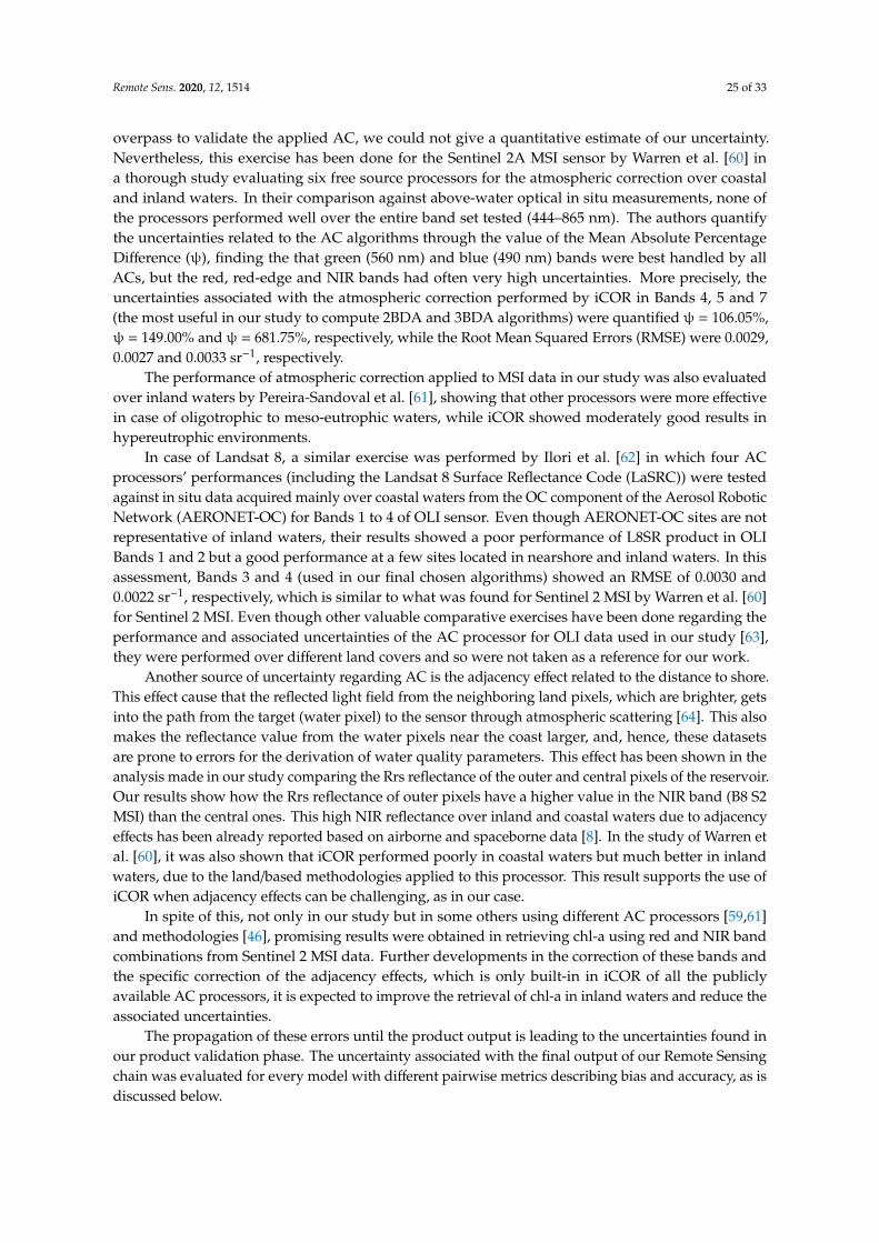
Remote Sens. 2020, 12, 1514 25 of 33

overpass to validate the applied AC, we could not give a quantitative estimate of our uncertainty.Nevertheless, this exercise has been done for the Sentinel 2A MSI sensor by Warren et al. [60] ina thorough study evaluating six free source processors for the atmospheric correction over coastaland inland waters. In their comparison against above-water optical in situ measurements, none ofthe processors performed well over the entire band set tested (444–865 nm). The authors quantifythe uncertainties related to the AC algorithms through the value of the Mean Absolute PercentageDifference (ψ), finding the that green (560 nm) and blue (490 nm) bands were best handled by allACs, but the red, red-edge and NIR bands had often very high uncertainties. More precisely, theuncertainties associated with the atmospheric correction performed by iCOR in Bands 4, 5 and 7(the most useful in our study to compute 2BDA and 3BDA algorithms) were quantified ψ = 106.05%,ψ = 149.00% and ψ = 681.75%, respectively, while the Root Mean Squared Errors (RMSE) were 0.0029,0.0027 and 0.0033 sr−1, respectively.

The performance of atmospheric correction applied to MSI data in our study was also evaluatedover inland waters by Pereira-Sandoval et al. [61], showing that other processors were more effectivein case of oligotrophic to meso-eutrophic waters, while iCOR showed moderately good results inhypereutrophic environments.

In case of Landsat 8, a similar exercise was performed by Ilori et al. [62] in which four ACprocessors’ performances (including the Landsat 8 Surface Reflectance Code (LaSRC)) were testedagainst in situ data acquired mainly over coastal waters from the OC component of the Aerosol RoboticNetwork (AERONET-OC) for Bands 1 to 4 of OLI sensor. Even though AERONET-OC sites are notrepresentative of inland waters, their results showed a poor performance of L8SR product in OLIBands 1 and 2 but a good performance at a few sites located in nearshore and inland waters. In thisassessment, Bands 3 and 4 (used in our final chosen algorithms) showed an RMSE of 0.0030 and0.0022 sr−1, respectively, which is similar to what was found for Sentinel 2 MSI by Warren et al. [60]for Sentinel 2 MSI. Even though other valuable comparative exercises have been done regarding theperformance and associated uncertainties of the AC processor for OLI data used in our study [63],they were performed over different land covers and so were not taken as a reference for our work.

Another source of uncertainty regarding AC is the adjacency effect related to the distance to shore.This effect cause that the reflected light field from the neighboring land pixels, which are brighter, getsinto the path from the target (water pixel) to the sensor through atmospheric scattering [64]. This alsomakes the reflectance value from the water pixels near the coast larger, and, hence, these datasetsare prone to errors for the derivation of water quality parameters. This effect has been shown in theanalysis made in our study comparing the Rrs reflectance of the outer and central pixels of the reservoir.Our results show how the Rrs reflectance of outer pixels have a higher value in the NIR band (B8 S2MSI) than the central ones. This high NIR reflectance over inland and coastal waters due to adjacencyeffects has been already reported based on airborne and spaceborne data [8]. In the study of Warren etal. [60], it was also shown that iCOR performed poorly in coastal waters but much better in inlandwaters, due to the land/based methodologies applied to this processor. This result supports the use ofiCOR when adjacency effects can be challenging, as in our case.

In spite of this, not only in our study but in some others using different AC processors [59,61]and methodologies [46], promising results were obtained in retrieving chl-a using red and NIR bandcombinations from Sentinel 2 MSI data. Further developments in the correction of these bands andthe specific correction of the adjacency effects, which is only built-in in iCOR of all the publiclyavailable AC processors, it is expected to improve the retrieval of chl-a in inland waters and reduce theassociated uncertainties.

The propagation of these errors until the product output is leading to the uncertainties found inour product validation phase. The uncertainty associated with the final output of our Remote Sensingchain was evaluated for every model with different pairwise metrics describing bias and accuracy, as isdiscussed below.

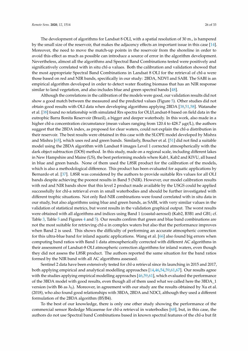
Remote Sens. 2020, 12, 1514 26 of 33

The development of algorithms for Landsat 8 OLI, with a spatial resolution of 30 m., is hamperedby the small size of the reservoir, that makes the adjacency effects an important issue in this case [14].Moreover, the need to move the match-up points in the reservoir from the shoreline in order toavoid this effect as much as possible can introduce a source of error in the algorithm development.Nevertheless, almost all the algorithms and Spectral Band Combinations tested were positively andsignificatively correlated with in situ chl-a values. Both the calibration and validation showed thatthe most appropriate Spectral Band Combinations in Landsat 8 OLI for the retrieval of chl-a werethose based on red and NIR bands, specifically in our study: 2BDA, NDVI and SABI. The SABI is anempirical algorithm developed in order to detect water floating biomass that has an NIR responsesimilar to land vegetation, and also includes blue and green spectral bands [48].

Although the correlations in the calibration of the models were good, our validation results did notshow a good match between the measured and the predicted values (Figure 5). Other studies did notobtain good results with OLI data when developing algorithms applying 2BDA [38,51,58]. Watanabeet al. [38] found no relationship with simulated Rrs spectra for OLI/Landsat-8 based on field data in theeutrophic Barra Bonita Reservoir (Brazil), a bigger and deeper waterbody. In this work, also made in ahigher chl-a concentration circumstance (mean values ranging from 120.4 to 428.7 µgr/L), the authorssuggest that the 2BDA index, as proposed for clear waters, could not explain the chl-a distribution intheir reservoir. The best results were obtained in this case with the SLOPE model developed by Mishraand Mishra [65], which uses red and green bands. Similarly, Boucher et al. [51] did not find a suitablemodel using the 2BDA algorithm with Landsat 8 images Level 1 corrected atmospherically with thedark object subtraction (DOS) method. In this study, made on a regional scale, including different lakesin New Hampshire and Maine (US), the best performing models where Kab1, Kab2 and KIVU, all basedin blue and green bands. None of them used the L8SR product for the calibration of the models,which is also a methodological difference. This product has been evaluated for aquatic applications byBernardo et al. [37]. L8SR was considered by the authors to provide suitable Rrs values for all OLIbands despite achieving the poorest results in Band 5 (NIR). However, our model calibration resultswith red and NIR bands show that this level 2 product made available by the USGS could be appliedsuccessfully for chl-a retrieval even in small waterbodies and should be further investigated withdifferent trophic situations. Not only Red-NIR combinations were found correlated with in situ data inour study, but also algorithms using blue and green bands, as SABI, with very similar values in thevalidation of statistical metrics, but worst results in the validation graphical output. The worst resultswere obtained with all algorithms and indices using Band 1 (coastal-aerosol) (Kab2, B3B1 and GB1; cf.Table 3, Table 5 and Figures 4 and 5). Our results confirm that green and blue band combinations arenot the most suitable for retrieving chl-a in complex waters but also that the performance improveswhen Band 2 is used. This shows the difficulty of performing an accurate atmospheric correctionfor this ultra-blue band for inland aquatic applications. Wang et al. [66] also found big errors whencomputing band ratios with Band 1 data atmospherically corrected with different AC algorithms intheir assessment of Landsat-8 OLI atmospheric correction algorithms for inland waters, even thoughthey did not assess the L8SR product. The authors reported the same situation for the band ratiosformed by the NIR band with all AC algorithms assessed.

Sentinel 2 data have been extensively tested for chl-a retrieval since its launching in 2015 and 2017,both applying empirical and analytical modelling approaches [14,46,54,59,61,67]. Our results agreewith the studies applying empirical modelling approaches [46,59,61], which evaluated the performanceof the 3BDA model with good results, even though all of them used what we called here the 3BDA_1version (with B6 as λ3). Moreover, in agreement with our study are the results obtained by Xu et al.(2018), who also found good relationships with 3BDA, 2BDA and NDCI, although they used a differentformulation of the 2BDA algorithm (B5/B4).

To the best of our knowledge, there is only one other study showing the performance of thecommercial sensor Rededge Micasense for chl-a retrieval in waterbodies [68], but, in this case, theauthors do not use Spectral band Combinations based in known spectral features of the chl-a but fit

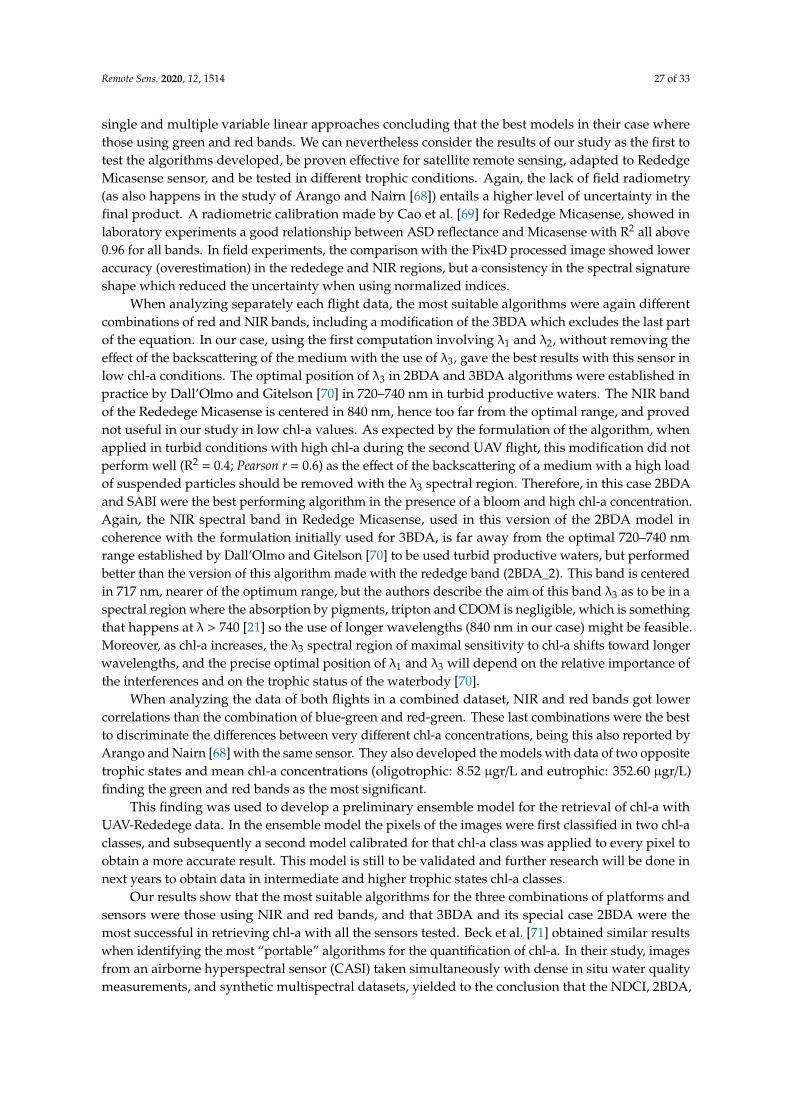
Remote Sens. 2020, 12, 1514 27 of 33

single and multiple variable linear approaches concluding that the best models in their case wherethose using green and red bands. We can nevertheless consider the results of our study as the first totest the algorithms developed, be proven effective for satellite remote sensing, adapted to RededgeMicasense sensor, and be tested in different trophic conditions. Again, the lack of field radiometry(as also happens in the study of Arango and Nairn [68]) entails a higher level of uncertainty in thefinal product. A radiometric calibration made by Cao et al. [69] for Rededge Micasense, showed inlaboratory experiments a good relationship between ASD reflectance and Micasense with R2 all above0.96 for all bands. In field experiments, the comparison with the Pix4D processed image showed loweraccuracy (overestimation) in the rededege and NIR regions, but a consistency in the spectral signatureshape which reduced the uncertainty when using normalized indices.

When analyzing separately each flight data, the most suitable algorithms were again differentcombinations of red and NIR bands, including a modification of the 3BDA which excludes the last partof the equation. In our case, using the first computation involving λ1 and λ2, without removing theeffect of the backscattering of the medium with the use of λ3, gave the best results with this sensor inlow chl-a conditions. The optimal position of λ3 in 2BDA and 3BDA algorithms were established inpractice by Dall’Olmo and Gitelson [70] in 720–740 nm in turbid productive waters. The NIR bandof the Rededege Micasense is centered in 840 nm, hence too far from the optimal range, and provednot useful in our study in low chl-a values. As expected by the formulation of the algorithm, whenapplied in turbid conditions with high chl-a during the second UAV flight, this modification did notperform well (R2 = 0.4; Pearson r = 0.6) as the effect of the backscattering of a medium with a high loadof suspended particles should be removed with the λ3 spectral region. Therefore, in this case 2BDAand SABI were the best performing algorithm in the presence of a bloom and high chl-a concentration.Again, the NIR spectral band in Rededge Micasense, used in this version of the 2BDA model incoherence with the formulation initially used for 3BDA, is far away from the optimal 720–740 nmrange established by Dall’Olmo and Gitelson [70] to be used turbid productive waters, but performedbetter than the version of this algorithm made with the rededge band (2BDA_2). This band is centeredin 717 nm, nearer of the optimum range, but the authors describe the aim of this band λ3 as to be in aspectral region where the absorption by pigments, tripton and CDOM is negligible, which is somethingthat happens at λ > 740 [21] so the use of longer wavelengths (840 nm in our case) might be feasible.Moreover, as chl-a increases, the λ3 spectral region of maximal sensitivity to chl-a shifts toward longerwavelengths, and the precise optimal position of λ1 and λ3 will depend on the relative importance ofthe interferences and on the trophic status of the waterbody [70].

When analyzing the data of both flights in a combined dataset, NIR and red bands got lowercorrelations than the combination of blue-green and red-green. These last combinations were the bestto discriminate the differences between very different chl-a concentrations, being this also reported byArango and Nairn [68] with the same sensor. They also developed the models with data of two oppositetrophic states and mean chl-a concentrations (oligotrophic: 8.52 µgr/L and eutrophic: 352.60 µgr/L)finding the green and red bands as the most significant.

This finding was used to develop a preliminary ensemble model for the retrieval of chl-a withUAV-Rededege data. In the ensemble model the pixels of the images were first classified in two chl-aclasses, and subsequently a second model calibrated for that chl-a class was applied to every pixel toobtain a more accurate result. This model is still to be validated and further research will be done innext years to obtain data in intermediate and higher trophic states chl-a classes.

Our results show that the most suitable algorithms for the three combinations of platforms andsensors were those using NIR and red bands, and that 3BDA and its special case 2BDA were themost successful in retrieving chl-a with all the sensors tested. Beck et al. [71] obtained similar resultswhen identifying the most “portable” algorithms for the quantification of chl-a. In their study, imagesfrom an airborne hyperspectral sensor (CASI) taken simultaneously with dense in situ water qualitymeasurements, and synthetic multispectral datasets, yielded to the conclusion that the NDCI, 2BDA,

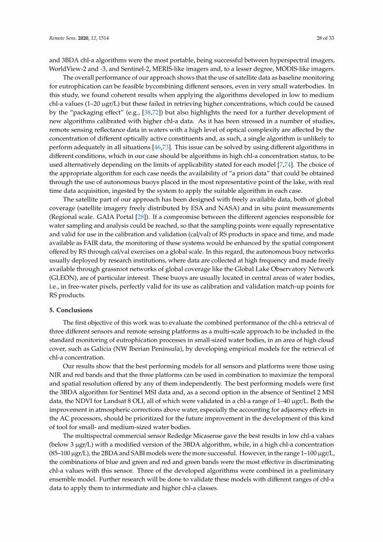
Remote Sens. 2020, 12, 1514 28 of 33

and 3BDA chl-a algorithms were the most portable, being successful between hyperspectral imagers,WorldView-2 and -3, and Sentinel-2, MERIS-like imagers and, to a lesser degree, MODIS-like imagers.

The overall performance of our approach shows that the use of satellite data as baseline monitoringfor eutrophication can be feasible bycombining different sensors, even in very small waterbodies. Inthis study, we found coherent results when applying the algorithms developed in low to mediumchl-a values (1–20 µgr/L) but these failed in retrieving higher concentrations, which could be causedby the “packaging effect” (e.g., [38,72]) but also highlights the need for a further development ofnew algorithms calibrated with higher chl-a data. As it has been stressed in a number of studies,remote sensing reflectance data in waters with a high level of optical complexity are affected by theconcentration of different optically active constituents and, as such, a single algorithm is unlikely toperform adequately in all situations [46,73]. This issue can be solved by using different algorithms indifferent conditions, which in our case should be algorithms in high chl-a concentration status, to beused alternatively depending on the limits of applicability stated for each model [7,74]. The choice ofthe appropriate algorithm for each case needs the availability of “a priori data” that could be obtainedthrough the use of autonomous buoys placed in the most representative point of the lake, with realtime data acquisition, ingested by the system to apply the suitable algorithm in each case.

The satellite part of our approach has been designed with freely available data, both of globalcoverage (satellite imagery freely distributed by ESA and NASA) and in situ point measurements(Regional scale. GAIA Portal [28]). If a compromise between the different agencies responsible forwater sampling and analysis could be reached, so that the sampling points were equally representativeand valid for use in the calibration and validation (cal/val) of RS products in space and time, and madeavailable as FAIR data, the monitoring of these systems would be enhanced by the spatial componentoffered by RS through cal/val exercises on a global scale. In this regard, the autonomous buoy networksusually deployed by research institutions, where data are collected at high frequency and made freelyavailable through grassroot networks of global coverage like the Global Lake Observatory Network(GLEON), are of particular interest. These buoys are usually located in central areas of water bodies,i.e., in free-water pixels, perfectly valid for its use as calibration and validation match-up points forRS products.

5. Conclusions

The first objective of this work was to evaluate the combined performance of the chl-a retrieval ofthree different sensors and remote sensing platforms as a multi-scale approach to be included in thestandard monitoring of eutrophication processes in small-sized water bodies, in an area of high cloudcover, such as Galicia (NW Iberian Peninsula), by developing empirical models for the retrieval ofchl-a concentration.

Our results show that the best performing models for all sensors and platforms were those usingNIR and red bands and that the three platforms can be used in combination to maximize the temporaland spatial resolution offered by any of them independently. The best performing models were firstthe 3BDA algorithm for Sentinel MSI data and, as a second option in the absence of Sentinel 2 MSIdata, the NDVI for Landsat 8 OLI, all of which were validated in a chl-a range of 1–40 µgr/L. Both theimprovement in atmospheric corrections above water, especially the accounting for adjacency effects inthe AC processors, should be prioritized for the future improvement in the development of this kindof tool for small- and medium-sized water bodies.

The multispectral commercial sensor Rededge Micasense gave the best results in low chl-a values(below 3 µgr/L) with a modified version of the 3BDA algorithm, while, in a high chl-a concentration(85–100µgr/L), the 2BDA and SABI models were the more successful. However, in the range 1–100µgr/L,the combinations of blue and green and red and green bands were the most effective in discriminatingchl-a values with this sensor. Three of the developed algorithms were combined in a preliminaryensemble model. Further research will be done to validate these models with different ranges of chl-adata to apply them to intermediate and higher chl-a classes.

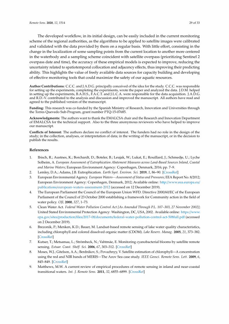
Remote Sens. 2020, 12, 1514 29 of 33

The developed workflow, in its initial design, can be easily included in the current monitoringscheme of the regional authorities, as the algorithms to be applied to satellite images were calibratedand validated with the data provided by them on a regular basis. With little effort, consisting in thechange in the localization of some sampling points from the current location to another more centeredin the waterbody and a sampling scheme coincident with satellite overpass (prioritizing Sentinel 2overpass date and time), the accuracy of these empirical models is expected to improve, reducing theuncertainty related to spatiotemporal collocation and adjacency effects, thus improving their predictingability. This highlights the value of freely available data sources for capacity building and developingof effective monitoring tools that could maximize the safety of our aquatic resources.

Author Contributions: C.C.C. and J.A.D.G. principally conceived of the idea for the study. C.C.C. was responsiblefor setting up the experiments, completing the experiments, wrote the paper and analyzed the data. J.D.M. helpedin setting up the experiments, B.A.H.S., F.A.C.T. and J.L.C.A. were responsible for the data acquisition. J.A.D.G.and R.D.-V. contributed to the analysis and discussion and improved the manuscript. All authors have read andagreed to the published version of the manuscript.

Funding: This research was co-funded by the Spanish Ministry of Research, Innovation and Universities throughthe Torres Quevedo Sub-Program, grant number PTQ-15-07685.

Acknowledgments: The authors want to thank the EMALCSA chair and the Research and Innovation Departmentof EMALCSA for the technical support. Also to the three anonymous reviewers who have helped to improveour manuscript.

Conflicts of Interest: The authors declare no conflict of interest. The funders had no role in the design of thestudy; in the collection, analyses, or interpretation of data; in the writing of the manuscript, or in the decision topublish the results.

References

1. Ibisch, R.; Austnes, K.; Borchardt, D.; Boteler, B.; Leujak, W.; Lukat, E.; Rouillard, J.; Schmedje, U.; LycheSolheim, A. European Assessment of Eutrophication Abatement Measures across Land-Based Sources Inland, Coastaland Marine Waters; European Environment Agency: Copenhagen, Denmark, 2016; pp. 7–9.

2. Lemley, D.A.; Adams, J.B. Eutrophication. Earth Syst. Environ. Sci. 2019, 1, 86–90. [CrossRef]3. European Environmental Agency. European Waters—Assessment of Status and Pressures; EEA Report No. 8/2012;

European Environment Agency: Copenhagen, Denmark, 2012; Available online: http://www.eea.europa.eu/

publications/european-waters-assessment-2012 (accessed on 12 December 2019).4. The European Parliament the Council of the European Union WFD. Directive 2000/60/EC of the European

Parliament of the Council of 23 October 2000 establishing a framework for Community action in the field ofwater policy. OJL 2000, 327, 1–73.

5. Clean Water Act. Federal Water Pollution Control Act [As Amended Through P.L. 107–303, 27 November 2002];United Stated Environmental Protection Agency: Washington, DC, USA, 2002. Available online: https://www.epa.gov/sites/production/files/2017-08/documents/federal-water-pollution-control-act-508full.pdf (accessedon 2 December 2019).

6. Brezonik, P.; Menken, K.D.; Bauer, M. Landsat-based remote sensing of lake water quality characteristics,including chlorophyll and colored dissolved organic matter (CDOM). Lake Reserv. Manag. 2005, 21, 373–382.[CrossRef]

7. Kutser, T.; Metsamaa, L.; Strömbeck, N.; Vahtmäe, E. Monitoring cyanobacterial blooms by satellite remotesensing. Estuar. Coast. Shelf. Sci. 2006, 67, 303–312. [CrossRef]

8. Moses, W.J.; Gitelson, A.A.; Berdnikov, S.; Povazhnyy, V. Satellite estimation of chlorophyll—A concentrationusing the red and NIR bands of MERIS—The Azov Sea case study. IEEE Geosci. Remote Sens. Lett. 2009, 6,845–849. [CrossRef]

9. Matthews, M.W. A current review of empirical procedures of remote sensing in inland and near-coastaltransitional waters. Int. J. Remote Sens. 2011, 32, 6855–6899. [CrossRef]

http://dx.doi.org/10.1016/B978-0-12-409548-9.10957-1

http://www.eea.europa.eu/publications/european-waters-assessment-2012

http://www.eea.europa.eu/publications/european-waters-assessment-2012

https://www.epa.gov/sites/production/files/2017-08/documents/federal-water-pollution-control-act-508full.pdf

https://www.epa.gov/sites/production/files/2017-08/documents/federal-water-pollution-control-act-508full.pdf

http://dx.doi.org/10.1080/07438140509354442

http://dx.doi.org/10.1016/j.ecss.2005.11.024

http://dx.doi.org/10.1109/LGRS.2009.2026657

http://dx.doi.org/10.1080/01431161.2010.512947

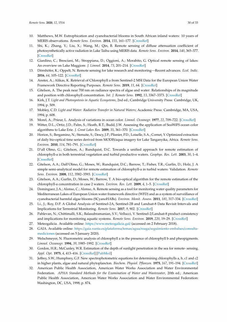
Remote Sens. 2020, 12, 1514 30 of 33

10. Matthews, M.W. Eutrophication and cyanobacterial blooms in South African inland waters: 10 years ofMERIS observations. Remote Sens. Environ. 2014, 155, 161–177. [CrossRef]

11. Shi, K.; Zhang, Y.; Liu, X.; Wang, M.; Qin, B. Remote sensing of diffuse attenuation coefficient ofphotosynthetically active radiation in Lake Taihu using MERIS data. Remote Sens. Environ. 2014, 140, 365–377.[CrossRef]

12. Giardino, C.; Bresciani, M.; Stroppiana, D.; Oggioni, A.; Morabito, G. Optical remote sensing of lakes:An overview on Lake Maggiore. J. Limnol. 2014, 73, 201–214. [CrossRef]

13. Dörnhöfer, K.; Oppelt, N. Remote sensing for lake research and monitoring—Recent advances. Ecol. Indic.2016, 64, 105–122. [CrossRef]

14. Anster, A.; Alikas, K. Retrieval of Chlorophyll a from Sentinel-2 MSI Data for the European Union WaterFramework Directive Reporting Purposes. Remote Sens. 2019, 11, 64. [CrossRef]

15. Gitelson, A. The peak near 700 nm on radiance spectra of algae and water: Relationships of its magnitudeand position with chlorophyll concentration. Int. J. Remote Sens. 1992, 13, 3367–3373. [CrossRef]

16. Kirk, J.T. Light and Photosyntesis in Aquatic Ecosystems, 2nd ed.; Cambridge University Press: Cambridge, UK,1994; p. 509.

17. Mobley, C.D. Light and Water: Radiative Transfer in Natural Waters; Academic Press: Cambridge, MA, USA,1994; p. 608.

18. Morel, A.; Prieur, L. Analysis of variations in ocean color. Limnol. Oceanogr. 1977, 22, 709–722. [CrossRef]19. Witter, D.L.; Ortiz, J.D.; Palm, S.; Heath, R.T.; Budd, J.W. Assessing the application of SeaWiFS ocean color

algorithms to Lake Erie. J. Great Lakes Res. 2009, 35, 361–370. [CrossRef]20. Horion, S.; Bergamino, N.; Stenuite, S.; Descy, J.P.; Plisnier, P.D.; Loiselle, S.A.; Cornet, Y. Optimized extraction

of daily bio-optical time series derived from MODIS/aqua imagery for Lake Tanganyika, Africa. Remote Sens.Environ. 2010, 114, 781–791. [CrossRef]

21. D’all Olmo, G.; Gitelson, A.; Rundquist, D.C. Towards a unified approach for remote estimation ofchlorophyll-a in both terrestrial vegetation and turbid productive waters. Geophys. Res. Lett. 2003, 30, 1–4.[CrossRef]

22. Gitelson, A.A.; Dall’Olmo, G.; Moses, W.; Rundquist, D.C.; Barrow, T.; Fisher, T.R.; Gurlin, D.; Holz, J. Asimple semi-analytical model for remote estimation of chlorophyll-a in turbid waters: Validation. RemoteSens. Environ. 2008, 112, 3582–3593. [CrossRef]

23. Gitelson, A.A.; Gurlin, D.; Moses, W.; Barrow, T. A bio-optical algorithm for the remote estimation of thechlorophyll-a concentration in case 2 waters. Environ. Res. Lett. 2009, 4, 1–5. [CrossRef]

24. Domínguez, J.A.; Alonso, C.; Alonso, A. Remote sensing as a tool for monitoring water quality parameters forMediterranean Lakes of European Union water framework directive (WFD) and as a system of surveillance ofcyanobacterial harmful algae blooms (SCyanoHABs). Environ. Monit. Assess. 2011, 181, 317–334. [CrossRef]

25. Li., J.; Roy, D.P. A Global Analysis of Sentinel-2A, Sentinel-2B and Landsat-8 Data Revisit Intervals andImplications for Terrestrial Monitoring. Remote Sens. 2017, 9, 902. [CrossRef]

26. Pahlevan, N.; Chittimalli, S.K.; Balasubramanian, S.V.; Vellucci, V. Sentinel-2/Landsat-8 product consistencyand implications for monitoring aquatic systems. Remote Sens. Environ. 2019, 220, 19–29. [CrossRef]

27. Meteogalicia. Available online: https://www.meteogalicia.gal/ (accessed on 2 February 2018).28. GAIA. Available online: https://gaia.xunta.es/plataforma/temas/agua/roaga/seguimiento-embalses/consulta-

mediciones (accessed on 5 January 2020).29. Welschmeyer, N. Fluorometric analysis of chlorophyll a in the presence of chlorophyll b and pheopigments.

Limnol. Oceanogr. 1994, 39, 1985–1992. [CrossRef]30. Gordon, H.R.; McCunley, W.R. Estimation of the depth of sunlight penetration in the sea for remotesensing.

Appl. Opt. 1975, 4, 413–416. [CrossRef] [PubMed]31. Jeffrey, S.W.; Humphrey, G.F. New spectrophotometric equations for determining chlorophylls a, b, c1 and c2

in higher plants, algae and natural phytoplancton. Biochem. Physiol. Pflanzen. 1975, 167, 191–194. [CrossRef]32. American Public Health Association, American Water Works Association and Water Environmental

Federation. APHA Standard Methods for the Examination of Water and Wastewater, 20th ed.; AmericanPublic Health Association, American Water Works Association and Water Environmental Federation:Washington, DC, USA, 1998; p. 874.

http://dx.doi.org/10.1016/j.rse.2014.08.010


http://dx.doi.org/10.4081/jlimnol.2014.817

http://dx.doi.org/10.1016/j.ecolind.2015.12.009

http://dx.doi.org/10.3390/rs11010064

http://dx.doi.org/10.1080/01431169208904125

http://dx.doi.org/10.4319/lo.1977.22.4.0709

http://dx.doi.org/10.1016/j.jglr.2009.03.002


http://dx.doi.org/10.1029/2003GL018065


http://dx.doi.org/10.1088/1748-9326/4/4/045003

http://dx.doi.org/10.1007/s10661-010-1831-7

http://dx.doi.org/10.3390/rs9090902


https://www.meteogalicia.gal/

https://gaia.xunta.es/plataforma/temas/agua/roaga/seguimiento-embalses/consulta-mediciones

https://gaia.xunta.es/plataforma/temas/agua/roaga/seguimiento-embalses/consulta-mediciones

http://dx.doi.org/10.4319/lo.1994.39.8.1985

http://dx.doi.org/10.1364/AO.14.000413

http://www.ncbi.nlm.nih.gov/pubmed/20134900

http://dx.doi.org/10.1016/S0015-3796(17)30778-3

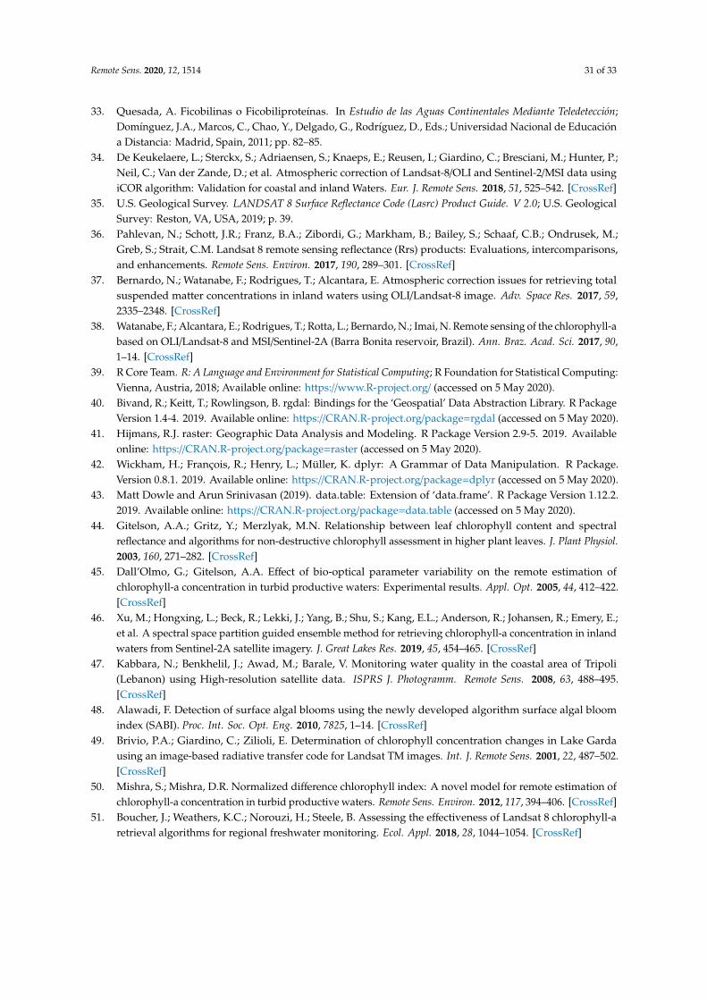
Remote Sens. 2020, 12, 1514 31 of 33

33. Quesada, A. Ficobilinas o Ficobiliproteínas. In Estudio de las Aguas Continentales Mediante Teledetección;Domínguez, J.A., Marcos, C., Chao, Y., Delgado, G., Rodríguez, D., Eds.; Universidad Nacional de Educacióna Distancia: Madrid, Spain, 2011; pp. 82–85.

34. De Keukelaere, L.; Sterckx, S.; Adriaensen, S.; Knaeps, E.; Reusen, I.; Giardino, C.; Bresciani, M.; Hunter, P.;Neil, C.; Van der Zande, D.; et al. Atmospheric correction of Landsat-8/OLI and Sentinel-2/MSI data usingiCOR algorithm: Validation for coastal and inland Waters. Eur. J. Remote Sens. 2018, 51, 525–542. [CrossRef]

35. U.S. Geological Survey. LANDSAT 8 Surface Reflectance Code (Lasrc) Product Guide. V 2.0; U.S. GeologicalSurvey: Reston, VA, USA, 2019; p. 39.

36. Pahlevan, N.; Schott, J.R.; Franz, B.A.; Zibordi, G.; Markham, B.; Bailey, S.; Schaaf, C.B.; Ondrusek, M.;Greb, S.; Strait, C.M. Landsat 8 remote sensing reflectance (Rrs) products: Evaluations, intercomparisons,and enhancements. Remote Sens. Environ. 2017, 190, 289–301. [CrossRef]

37. Bernardo, N.; Watanabe, F.; Rodrigues, T.; Alcantara, E. Atmospheric correction issues for retrieving totalsuspended matter concentrations in inland waters using OLI/Landsat-8 image. Adv. Space Res. 2017, 59,2335–2348. [CrossRef]

38. Watanabe, F.; Alcantara, E.; Rodrigues, T.; Rotta, L.; Bernardo, N.; Imai, N. Remote sensing of the chlorophyll-abased on OLI/Landsat-8 and MSI/Sentinel-2A (Barra Bonita reservoir, Brazil). Ann. Braz. Acad. Sci. 2017, 90,1–14. [CrossRef]

39. R Core Team. R: A Language and Environment for Statistical Computing; R Foundation for Statistical Computing:Vienna, Austria, 2018; Available online: https://www.R-project.org/ (accessed on 5 May 2020).

40. Bivand, R.; Keitt, T.; Rowlingson, B. rgdal: Bindings for the ‘Geospatial’ Data Abstraction Library. R PackageVersion 1.4-4. 2019. Available online: https://CRAN.R-project.org/package=rgdal (accessed on 5 May 2020).

41. Hijmans, R.J. raster: Geographic Data Analysis and Modeling. R Package Version 2.9-5. 2019. Availableonline: https://CRAN.R-project.org/package=raster (accessed on 5 May 2020).

42. Wickham, H.; François, R.; Henry, L.; Müller, K. dplyr: A Grammar of Data Manipulation. R Package.Version 0.8.1. 2019. Available online: https://CRAN.R-project.org/package=dplyr (accessed on 5 May 2020).

43. Matt Dowle and Arun Srinivasan (2019). data.table: Extension of ‘data.frame’. R Package Version 1.12.2.2019. Available online: https://CRAN.R-project.org/package=data.table (accessed on 5 May 2020).

44. Gitelson, A.A.; Gritz, Y.; Merzlyak, M.N. Relationship between leaf chlorophyll content and spectralreflectance and algorithms for non-destructive chlorophyll assessment in higher plant leaves. J. Plant Physiol.2003, 160, 271–282. [CrossRef]

45. Dall’Olmo, G.; Gitelson, A.A. Effect of bio-optical parameter variability on the remote estimation ofchlorophyll-a concentration in turbid productive waters: Experimental results. Appl. Opt. 2005, 44, 412–422.[CrossRef]

46. Xu, M.; Hongxing, L.; Beck, R.; Lekki, J.; Yang, B.; Shu, S.; Kang, E.L.; Anderson, R.; Johansen, R.; Emery, E.;et al. A spectral space partition guided ensemble method for retrieving chlorophyll-a concentration in inlandwaters from Sentinel-2A satellite imagery. J. Great Lakes Res. 2019, 45, 454–465. [CrossRef]

47. Kabbara, N.; Benkhelil, J.; Awad, M.; Barale, V. Monitoring water quality in the coastal area of Tripoli(Lebanon) using High-resolution satellite data. ISPRS J. Photogramm. Remote Sens. 2008, 63, 488–495.[CrossRef]

48. Alawadi, F. Detection of surface algal blooms using the newly developed algorithm surface algal bloomindex (SABI). Proc. Int. Soc. Opt. Eng. 2010, 7825, 1–14. [CrossRef]

49. Brivio, P.A.; Giardino, C.; Zilioli, E. Determination of chlorophyll concentration changes in Lake Gardausing an image-based radiative transfer code for Landsat TM images. Int. J. Remote Sens. 2001, 22, 487–502.[CrossRef]

50. Mishra, S.; Mishra, D.R. Normalized difference chlorophyll index: A novel model for remote estimation ofchlorophyll-a concentration in turbid productive waters. Remote Sens. Environ. 2012, 117, 394–406. [CrossRef]

51. Boucher, J.; Weathers, K.C.; Norouzi, H.; Steele, B. Assessing the effectiveness of Landsat 8 chlorophyll-aretrieval algorithms for regional freshwater monitoring. Ecol. Appl. 2018, 28, 1044–1054. [CrossRef]

http://dx.doi.org/10.1080/22797254.2018.1457937


http://dx.doi.org/10.1016/j.asr.2017.02.017

http://dx.doi.org/10.1590/0001-3765201720170125

https://www.R-project.org/

https://CRAN.R-project.org/package=rgdal

https://CRAN.R-project.org/package=raster

https://CRAN.R-project.org/package=dplyr

https://CRAN.R-project.org/package=data.table

http://dx.doi.org/10.1078/0176-1617-00887

http://dx.doi.org/10.1364/AO.44.000412

http://dx.doi.org/10.1016/j.jglr.2018.09.002

http://dx.doi.org/10.1016/j.isprsjprs.2008.01.004

http://dx.doi.org/10.1117/12.862096

http://dx.doi.org/10.1080/014311601450059


http://dx.doi.org/10.1002/eap.1708

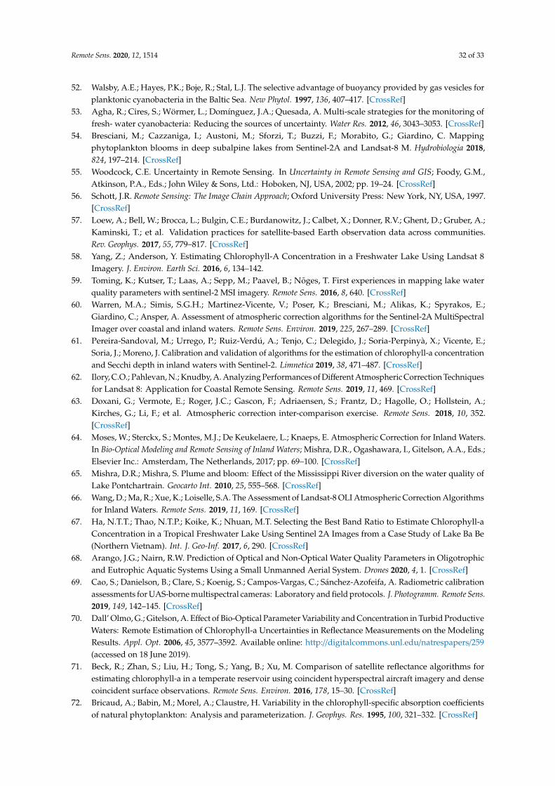
Remote Sens. 2020, 12, 1514 32 of 33

52. Walsby, A.E.; Hayes, P.K.; Boje, R.; Stal, L.J. The selective advantage of buoyancy provided by gas vesicles forplanktonic cyanobacteria in the Baltic Sea. New Phytol. 1997, 136, 407–417. [CrossRef]

53. Agha, R.; Cires, S.; Wörmer, L.; Domínguez, J.A.; Quesada, A. Multi-scale strategies for the monitoring offresh- water cyanobacteria: Reducing the sources of uncertainty. Water Res. 2012, 46, 3043–3053. [CrossRef]

54. Bresciani, M.; Cazzaniga, I.; Austoni, M.; Sforzi, T.; Buzzi, F.; Morabito, G.; Giardino, C. Mappingphytoplankton blooms in deep subalpine lakes from Sentinel-2A and Landsat-8 M. Hydrobiologia 2018,824, 197–214. [CrossRef]

55. Woodcock, C.E. Uncertainty in Remote Sensing. In Uncertainty in Remote Sensing and GIS; Foody, G.M.,Atkinson, P.A., Eds.; John Wiley & Sons, Ltd.: Hoboken, NJ, USA, 2002; pp. 19–24. [CrossRef]

56. Schott, J.R. Remote Sensing: The Image Chain Approach; Oxford University Press: New York, NY, USA, 1997.[CrossRef]

57. Loew, A.; Bell, W.; Brocca, L.; Bulgin, C.E.; Burdanowitz, J.; Calbet, X.; Donner, R.V.; Ghent, D.; Gruber, A.;Kaminski, T.; et al. Validation practices for satellite-based Earth observation data across communities.Rev. Geophys. 2017, 55, 779–817. [CrossRef]

58. Yang, Z.; Anderson, Y. Estimating Chlorophyll-A Concentration in a Freshwater Lake Using Landsat 8Imagery. J. Environ. Earth Sci. 2016, 6, 134–142.

59. Toming, K.; Kutser, T.; Laas, A.; Sepp, M.; Paavel, B.; Nõges, T. First experiences in mapping lake waterquality parameters with sentinel-2 MSI imagery. Remote Sens. 2016, 8, 640. [CrossRef]

60. Warren, M.A.; Simis, S.G.H.; Martinez-Vicente, V.; Poser, K.; Bresciani, M.; Alikas, K.; Spyrakos, E.;Giardino, C.; Ansper, A. Assessment of atmospheric correction algorithms for the Sentinel-2A MultiSpectralImager over coastal and inland waters. Remote Sens. Environ. 2019, 225, 267–289. [CrossRef]

61. Pereira-Sandoval, M.; Urrego, P.; Ruiz-Verdú, A.; Tenjo, C.; Delegido, J.; Soria-Perpinyà, X.; Vicente, E.;Soria, J.; Moreno, J. Calibration and validation of algorithms for the estimation of chlorophyll-a concentrationand Secchi depth in inland waters with Sentinel-2. Limnetica 2019, 38, 471–487. [CrossRef]

62. Ilory, C.O.; Pahlevan, N.; Knudby, A. Analyzing Performances of Different Atmospheric Correction Techniquesfor Landsat 8: Application for Coastal Remote Sensing. Remote Sens. 2019, 11, 469. [CrossRef]

63. Doxani, G.; Vermote, E.; Roger, J.C.; Gascon, F.; Adriaensen, S.; Frantz, D.; Hagolle, O.; Hollstein, A.;Kirches, G.; Li, F.; et al. Atmospheric correction inter-comparison exercise. Remote Sens. 2018, 10, 352.[CrossRef]

64. Moses, W.; Sterckx, S.; Montes, M.J.; De Keukelaere, L.; Knaeps, E. Atmospheric Correction for Inland Waters.In Bio-Optical Modeling and Remote Sensing of Inland Waters; Mishra, D.R., Ogashawara, I., Gitelson, A.A., Eds.;Elsevier Inc.: Amsterdam, The Netherlands, 2017; pp. 69–100. [CrossRef]

65. Mishra, D.R.; Mishra, S. Plume and bloom: Effect of the Mississippi River diversion on the water quality ofLake Pontchartrain. Geocarto Int. 2010, 25, 555–568. [CrossRef]

66. Wang, D.; Ma, R.; Xue, K.; Loiselle, S.A. The Assessment of Landsat-8 OLI Atmospheric Correction Algorithmsfor Inland Waters. Remote Sens. 2019, 11, 169. [CrossRef]

67. Ha, N.T.T.; Thao, N.T.P.; Koike, K.; Nhuan, M.T. Selecting the Best Band Ratio to Estimate Chlorophyll-aConcentration in a Tropical Freshwater Lake Using Sentinel 2A Images from a Case Study of Lake Ba Be(Northern Vietnam). Int. J. Geo-Inf. 2017, 6, 290. [CrossRef]

68. Arango, J.G.; Nairn, R.W. Prediction of Optical and Non-Optical Water Quality Parameters in Oligotrophicand Eutrophic Aquatic Systems Using a Small Unmanned Aerial System. Drones 2020, 4, 1. [CrossRef]

69. Cao, S.; Danielson, B.; Clare, S.; Koenig, S.; Campos-Vargas, C.; Sánchez-Azofeifa, A. Radiometric calibrationassessments for UAS-borne multispectral cameras: Laboratory and field protocols. J. Photogramm. Remote Sens.2019, 149, 142–145. [CrossRef]

70. Dall’ Olmo, G.; Gitelson, A. Effect of Bio-Optical Parameter Variability and Concentration in Turbid ProductiveWaters: Remote Estimation of Chlorophyll-a Uncertainties in Reflectance Measurements on the ModelingResults. Appl. Opt. 2006, 45, 3577–3592. Available online: http://digitalcommons.unl.edu/natrespapers/259(accessed on 18 June 2019).

71. Beck, R.; Zhan, S.; Liu, H.; Tong, S.; Yang, B.; Xu, M. Comparison of satellite reflectance algorithms forestimating chlorophyll-a in a temperate reservoir using coincident hyperspectral aircraft imagery and densecoincident surface observations. Remote Sens. Environ. 2016, 178, 15–30. [CrossRef]

72. Bricaud, A.; Babin, M.; Morel, A.; Claustre, H. Variability in the chlorophyll-specific absorption coefficientsof natural phytoplankton: Analysis and parameterization. J. Geophys. Res. 1995, 100, 321–332. [CrossRef]

http://dx.doi.org/10.1046/j.1469-8137.1997.00754.x

http://dx.doi.org/10.1016/j.watres.2012.03.005

http://dx.doi.org/10.1007/s10750-017-3462-2

http://dx.doi.org/10.1002/0470035269

http://dx.doi.org/10.5860/choice.45-0889

http://dx.doi.org/10.1002/2017RG000562

http://dx.doi.org/10.3390/rs8080640


http://dx.doi.org/10.23818/limn.38.27

http://dx.doi.org/10.3390/rs11040469

http://dx.doi.org/10.3390/rs10020352

http://dx.doi.org/10.1016/B978-0-12-804644-9.00003-3

http://dx.doi.org/10.1080/10106041003763394

http://dx.doi.org/10.3390/rs11020169

http://dx.doi.org/10.3390/ijgi6090290

http://dx.doi.org/10.3390/drones4010001

http://dx.doi.org/10.1016/j.isprsjprs.2019.01.016

http://digitalcommons.unl.edu/natrespapers/259


http://dx.doi.org/10.1029/95JC00463

Remote Sens. 2020, 12, 1514 33 of 33

73. Tyler, A.; Hunter, P.D.; Spyrakos, E.; Groomb, E.; Constantinescu, A.M.; Kitchen, J. Developments in Earthobservation for the assessment and monitoring of inland, transitional, coastal and shelf-sea waters. Sci. TotalEnviron. 2016, 572, 1307–1321. [CrossRef] [PubMed]

74. Stumpf, R.P.; Tyler, M.A. Satellite detection of bloom and pigment distributions in estuaries. Remote Sens.Environ. 1988, 24, 385–404. [CrossRef]

© 2020 by the authors. Licensee MDPI, Basel, Switzerland. This article is an open accessarticle distributed under the terms and conditions of the Creative Commons Attribution(CC BY) license (http://creativecommons.org/licenses/by/4.0/).

http://dx.doi.org/10.1016/j.scitotenv.2016.01.020

http://www.ncbi.nlm.nih.gov/pubmed/26805447

http://dx.doi.org/10.1016/0034-4257(88)90014-4

http://creativecommons.org/

http://creativecommons.org/licenses/by/4.0/.

an uav and satellite multispectral data approach to

Documents