analele universitĂŢii “dunĂrea de jos” din galaŢi€¦ · · 2010-06-18ria—the guide...
TRANSCRIPT

MINISTERU
ANAL “DUNĂR
Fascicula X
MECANICĂ APLIC
A
MINISTRY O
THE ANNAUNIV
Fascicle X
APPLIED MECHA
Y
L EDUCAŢIEI SI CERCETĂRII
ELE UNIVERSITĂŢII EA DE JOS” DIN GALAŢI
ATĂ
NUL XXV (XXX) 2007
ISSN 1221-4612
F EDUCATION AND RESEARCH
LS OF “DUNAREA DE JOS” ERSITY OF GALATI
NICS
EAR XXV (XXX) 2007 ISSN 1221-4612

Manuscripts, reviews and books for an exchange cooperation, as well as any correspondence will be mailed to:
THE ANNALS OF GALATI UNIVERSITY
UNIVERSITATEA "DUNĂREA DE JOS" DIN GALAŢI
REDACŢIA ANALELOR
Fax 40 236 46 13 53
Str. Domneasca nr. 47
800008 Galaţi
ROMANIA

EDITING MANAGEMENT
RESPONSIBLE EDITOR: Professor VIOREL MINZU
MEMBERS: Professor TEODOR MUNTEANU Professor DANIELA SARPE Professor MIRELA PRAISLER Professor ANCA GATA ASSISTANT EDITOR: Assoc. Professor ALEXANDRU IOAN
EDITING STAFF
FASCICLE X APPLIED MECHANICS YEAR XXIV (XXX) 2007
EDITOR IN CHIEF: Professor IONEL CHIRICA
Tel: 40 236 414871 Fax: 40 236 314463
e-mail: [email protected]
MEMBERS: Professor SORIN D. MUSAT, University “Dunarea de Jos” of Galati Professor LIVIU D. STOICESCU, University “Dunarea de Jos” of Galati Professor IORDAN MATULEA, University “Dunarea de Jos” of Galati Professor IORDAN MATULEA, University “Dunarea de Jos” of Galati Professor EUGEN RUSU, University “Dunarea de Jos” of Galati Professor CARLOS GUEDES SOARES, IST, Technical University of Lisbon Professor R. AJIT SHENOI, University of Southampton, UK Professor PURNENDU K. DAS, University of Glasgow, UK Professor PHILIPPE RIGO, University of Liege, Belgium Professor DAVID HUI, University of New Orleans, USA ASSISTANT EDITOR : Ass. Professor ELENA F. BEZNEA, University “Dunarea de Jos” of Galati

_________________________________________________________________________________________________________________ ANALELE UNIVERSITATII „DUNAREA DE JOS” DIN GALATI
Fascicula X - MECANICA APLICATA, ISSN 1221-4612 Anul 2007
MECANICA APLICATA CUPRINS
I.CHIRICA, E.F.BEZNEA, R.CHIRICA, V. GIUGLEA, PH. RIGO. Metodologii de calcul la oboseala a structurilor de nave ................................................................................................................................ 7 S.D.MUSAT, L.C.RUSU. Equatii Lagrange cu multiplicatori pentru corpuri rigide............................................ 13 S.D.MUSAT, L.C.RUSU. Studiul torsiunii in sistemele cu ramificatii care transmit miscare de rotati ............... 19 L.C.RUSU. Performante obtinute cu modele de spectre de val de a 3-a generatie in Marea Neagra.................... 23 S.D.MUSAT, D. BOAZU. Vibratii fortate in sisteme de arbori cu roti dintate .................................................... 33 D.BOAZU. Poiectarea formei pentru problemele de contact elastic ..................................................................... 39 E.RUSU. Un program MATLAB pentru modelarea sprectrelor de val................................................................. 45 G.C.BALAN, A.EPUREANU. Detectia Chatter prin utilizarea Fortei principale de taiere (Prima parte)............ 53 E.F.BEZNEA, I.CHIRICA, R.CHIRICA. Pierderea stabilitatii panourilor compozite cu imperfectiuni initiale .. 57 R.CHIRICA, S.D. MUSAT, E.F.BEZNEA. Analiza vibratiilor torsionale ale unui model de nava de tip portcontainer, confectionat din materiale compozite............................................................................................. 63
APPLIED MECHANICS
CONTENTS I.CHIRICA, E.F.BEZNEA, R.CHIRICA, V. GIUGLEA , PH. RIGO. Methodologies for ship structures fatigue life assessment............................................................................................................................................. 7 S.D.MUSAT, L.C.RUSU. Lagrange Equations with Multipliers for the Rigid Body........................................... 13 S.D.MUSAT, L.C.RUSU. Study of Torsion in the Systems with Ramifications for Transmitting the Rotation Motion .................................................................................................................................................... 19 L.C.RUSU. On the Performances of the Third Generation Spectral Wave Models in the Black Sea ................... 23 S.D.MUSAT, D. BOAZU. Forced vibrations in geared shaft systems.................................................................. 33 D.BOAZU. Shape Design For Elastic Contact Problems...................................................................................... 39 E.RUSU. A MATLAB Toolbox Associated with Spectral Wave Modelling ....................................................... 45 G.C.BALAN, A.EPUREANU. Chatter Detection Using the Main Cutting Force (1-st Part) ............................... 53 E.F.BEZNEA, I.CHIRICA, R.CHIRICA. Buckling of composite panels with initial imperfection ..................... 57 R.CHIRICA, S.D. MUSAT, E.F.BEZNEA. Torsional vibration analysis of a container-ship hull model, made of composite materials ................................................................................................................................. 63

THE ANNALS OF “DUNAREA DE JOS” UNIVERSITY OF GALATI FASCICLE X APPLIED MECHANICS, ISSN 1221-4612
2007
I t s iI G
K
The fing cathe crgrowsof strpredicT-joinjointssurfacof thstressIn thstressproparaw dFatigucrackFor mmajorsels a[1], ntivelystrengtigue dama(tankewere only 3
n the
Methodologies for Ship Structures Fatigue Life Assessment
Ionel Chirică, Elena-Felicia Beznea, Raluca Chirică “Dunarea de Jos” University of Galati
Vasile Giuglea Ship Design Group
Philippe Rigo University of Liege
ABSTRACT
n the paper, the analysis of the methodologies for ship structures fatigue life assessment isreated. In fact, the fatigue life determination, by using usage factor of the ship decktructure is the main aim of the paper. In the paper are exposed certain methodologiesusedn ship structural analysis. The work was made within the European Project PC6-MPROVE, (https://improve.bal-pm.com/) which has been financed by the EU through theROWTH Programme, under Contract No. FP6-03138.
EY WORDS F ti hi t t
sion or wastage. The cracks occurred mostly o
1. Introductionatigue life of a structure under repeated load-n be divided into the crack initiation life and ack propagation life where the initiated crack to a certain point where it affects the safety
ucture. The purpose of this investigation is to t the theoretical macro crack propagation in a t and a Hopper knuckle, typical welding
in vessels, using stress intensity factors. The e cracks that initiate and propagate at the toe
e welding area are affected by the residual es that are created during the welding process. is experiment, an effect of these residual es was reflected on the analysis of the crack gation, and it was compared with the actual ata. e is responsible for a large proportion of
s occurring in welded ship structural details. any years fatigue related failure has become a concern in the maintenance of existing ves-nd the design of new vessels. As reported in umerous cracks were experienced by rela- new oil carriers constructed of higher-th materials. As indicated, more than 10 fa-cracks per damaged ship were found during ge surveys of 48 "second generation" VLCCs r class) using E32 and E36 steels. The cracks discovered when the ships were, on average, to 4 years old without any significant corro-
side longitudinals at the connections to transverse bulkheads or transverse webs. Fatigue cracks were also reported on other types of vessels. For exam-ple, in some bulk carriers, cracks were commonly found in the "hard" corners of the lower hopper tanks connecting to the side frames, and the lower stools connecting to the double bottom. It is important to note that the fatigue strength of welded structural details (with stress concentration) is not dependent on the tensile strength of the steel. Fatigue refers to the failure of materials under re-peated actions of stress fluctuation. The loads re-sponsible for fatigue are generally not large enough to cause material yielding. Instead, failure occurs after a certain number of load or stress fluctuations. Two distinct features, typical of high-cycle fatigue, are generally seen on the cracked surfaces of fa-tigue failure of ship structures: 1) the material has undergone only minor yielding, and the strain was essentially elastic, 2) the fracture surface is smooth, with characteristic chevron lines reflecting the variable intensity of loading of low and high sea states during the ves-sel's service life. The American Bureau of Shipping (ABS) has over the years devoted considerable effort in the devel-opment of the SafeHull system to cope with the assessment of yielding, ultimate strength and fa-tigue of hull structures. ABS SafeHull is a dynamic
7
FASCICLE X THE ANNALS OF “DUNAREA DE JOS” UNIVERSITY OF GALATI __________________________________________________________________________ based design and analysis tool. To provide a practi-cal tool for fatigue strength assessment, the Safe-Hull approach is based on the so-called “Simplified Fatigue”.
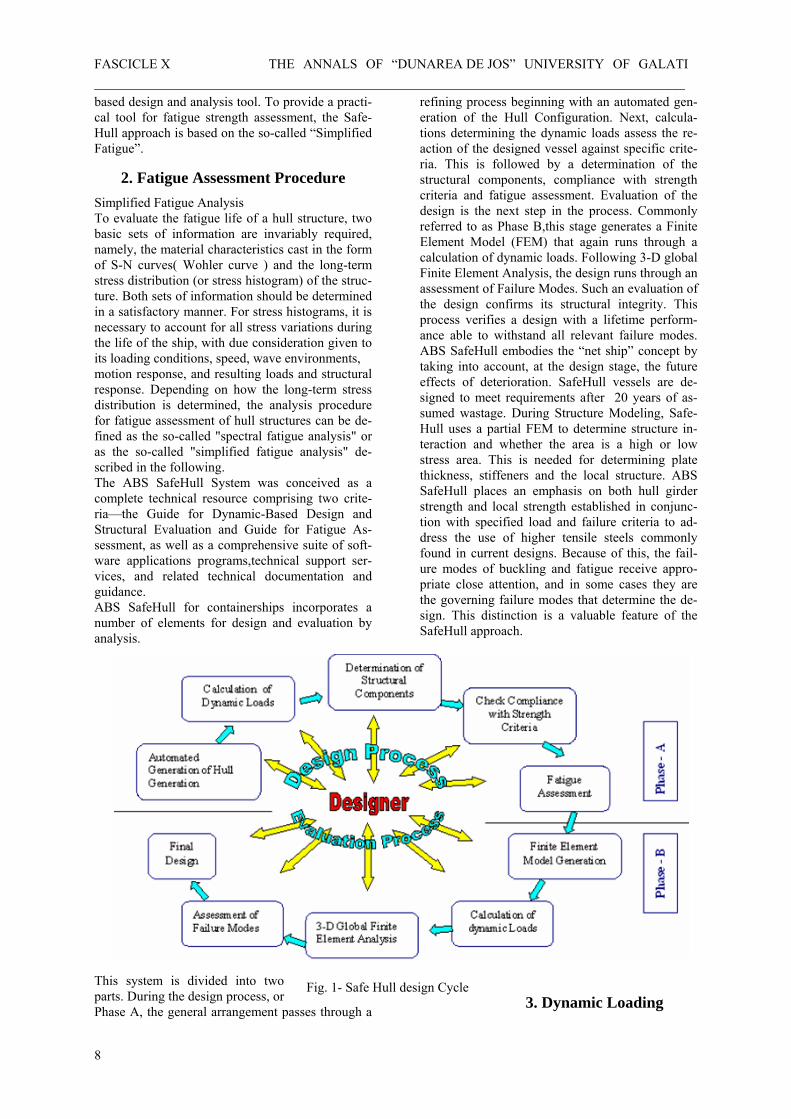
2. Fatigue Assessment Procedure Simplified Fatigue Analysis To evaluate the fatigue life of a hull structure, two basic sets of information are invariably required, namely, the material characteristics cast in the form of S-N curves( Wohler curve ) and the long-term stress distribution (or stress histogram) of the struc-ture. Both sets of information should be determined in a satisfactory manner. For stress histograms, it is necessary to account for all stress variations during the life of the ship, with due consideration given to its loading conditions, speed, wave environments, motion response, and resulting loads and structural response. Depending on how the long-term stress distribution is determined, the analysis procedure for fatigue assessment of hull structures can be de-fined as the so-called "spectral fatigue analysis" or as the so-called "simplified fatigue analysis" de-scribed in the following. The ABS SafeHull System was conceived as a complete technical resource comprising two crite-ria—the Guide for Dynamic-Based Design and Structural Evaluation and Guide for Fatigue As-sessment, as well as a comprehensive suite of soft-ware applications programs,technical support ser-vices, and related technical documentation and guidance. ABS SafeHull for containerships incorporates a number of elements for design and evaluation by analysis.
This system is divided into two parts. During the design process, or Phase A, the general arrangement passes through a
refining process beginning with an automated gen-eration of the Hull Configuration. Next, calcula-tions determining the dynamic loads assess the re-action of the designed vessel against specific crite-ria. This is followed by a determination of the structural components, compliance with strength criteria and fatigue assessment. Evaluation of the design is the next step in the process. Commonly referred to as Phase B,this stage generates a Finite Element Model (FEM) that again runs through a calculation of dynamic loads. Following 3-D global Finite Element Analysis, the design runs through an assessment of Failure Modes. Such an evaluation of the design confirms its structural integrity. This process verifies a design with a lifetime perform-ance able to withstand all relevant failure modes. ABS SafeHull embodies the “net ship” concept by taking into account, at the design stage, the future effects of deterioration. SafeHull vessels are de-signed to meet requirements after 20 years of as-sumed wastage. During Structure Modeling, Safe-Hull uses a partial FEM to determine structure in-teraction and whether the area is a high or low stress area. This is needed for determining plate thickness, stiffeners and the local structure. ABS SafeHull places an emphasis on both hull girder strength and local strength established in conjunc-tion with specified load and failure criteria to ad-dress the use of higher tensile steels commonly found in current designs. Because of this, the fail-ure modes of buckling and fatigue receive appro-priate close attention, and in some cases they are the governing failure modes that determine the de-sign. This distinction is a valuable feature of the SafeHull approach.
3. Dynamic Loading Fig. 1- Safe Hull design Cycle
8
THE ANNALS OF “DUNAREA DE JOS” UNIVERSITY OF GALATI FASCICLE X ___________________________________________________________________________
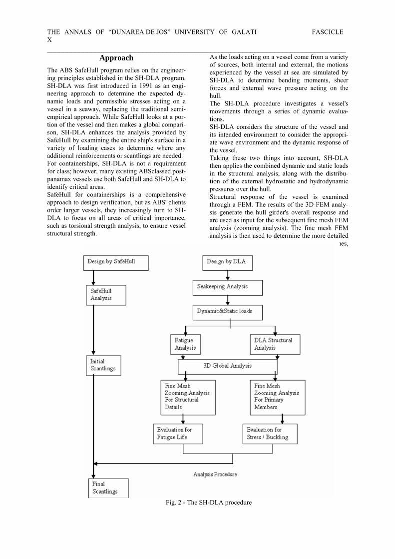
Approach The ABS SafeHull program relies on the engineer-ing principles established in the SH-DLA program. SH-DLA was first introduced in 1991 as an engi-neering approach to determine the expected dy-namic loads and permissible stresses acting on a vessel in a seaway, replacing the traditional semi-empirical approach. While SafeHull looks at a por-tion of the vessel and then makes a global compari-son, SH-DLA enhances the analysis provided by SafeHull by examining the entire ship's surface in a variety of loading cases to determine where any additional reinforcements or scantlings are needed. For containerships, SH-DLA is not a requirement for class; however, many existing ABSclassed post-panamax vessels use both SafeHull and SH-DLA to identify critical areas. SafeHull for containerships is a comprehensive approach to design verification, but as ABS' clients order larger vessels, they increasingly turn to SH-DLA to focus on all areas of critical importance, such as torsional strength analysis, to ensure vessel structural strength.
As the loads acting on a vessel come from a variety of sources, both internal and external, the motions experienced by the vessel at sea are simulated by SH-DLA to determine bending moments, sheer forces and external wave pressure acting on the hull. The SH-DLA procedure investigates a vessel's movements through a series of dynamic evalua-tions. SH-DLA considers the structure of the vessel and its intended environment to consider the appropri-ate wave environment and the dynamic response of the vessel. Taking these two things into account, SH-DLA then applies the combined dynamic and static loads in the structural analysis, along with the distribu-tion of the external hydrostatic and hydrodynamic pressures over the hull. Structural response of the vessel is examined through a FEM. The results of the 3D FEM analy-sis generate the hull girder's overall response and are used as input for the subsequent fine mesh FEM analysis (zooming analysis). The fine mesh FEM analysis is then used to determine the more detailed local stresses, including transverse web frames, longitudinal girders, and all horizontal stringers.
Fig. 2 - The SH-DLA procedure

FASCICLE X THE ANNALS OF “DUNAREA DE JOS” UNIVERSITY OF GALATI __________________________________________________________________________ These FEM results are then used to examine the stresses and deflections in the structure to ensure they fall within the prescribed limits of the failure modes of yield and buckling. The greater detail of SH-DLA provides further assurance to a robust design with a long service life. SH-DLA represents a consistent and rational ap-proach that employs a direct linear analysis of the containership. This reduces the "modeling uncer-tainties" that may be introduced when using rule scantling equations. Rule equations have necessar-ily relied on simplifications to account for the ap-plied loads, structural response and strength. The comprehensive SH-DLA analysis does not rely on these modeling simplifications and produces more reliable answers for structural components. Just as SH-DLA can be used to further verify spe-cific load cases, ABS employs a variety of other analyses to refine designs against known influ-ences.
4. Loads and Strength Assessment To obtain the combined load effects, a comprehen-sive set of design load cases has been developed to ensure that the maximum response has been con-sidered by analyzing the Hydrodynamic Loads, Impact Loads, Ballast Loads, Container Loads, and Operational Loads. Loading cases are used to de-termine the effect of green water on deck and on hatch covers. Loads are calculated to determine the proper scantlings in a rational manner for the fore-body. The torsional strength of the hull and high stress concentrations at the hatch corners are of paramount concern. Oblique sea conditions are applied to impose maximum torsional loads at the forward and aft ends of the mid-ship cargo hold and to check the fatigue strength of the structures immediately forward of the engine room where there is an abrupt change in torsional rigidity. ABS SafeHull encompasses a strength assessment to verify the suitability of the initial design, against the specified failure criteria. A series of load cases are specified to determine the scantlings against yielding strength, buckling and ultimate strength, and fatigue strength of the material. Of particular importance to containerships is the design of hatch openings concerning associated loads, stresses and distortions. The large deck openings, the strong warping restraint of the engine room, and the non-prismatic hull structure of con-tainerships cause significant torsion-induced longi-tudinal warping stresses along the strength deck. Certain structural details have been identified as particularly vulnerable to fatigue. Special attention in the development of the SafeHull criteria has been given to the following fatigue sensitive areas: Hatch corners on the main and second decks, and top of continuous hatchside coamings
Connections of longitudinal deck girders to trans-verse bulkheads, and side longitudinals to webs and transverse bulkheads End connections for the hatch side coaming, in-cluding coaming stays and hatch end coamings Cutouts in the longitudinal bulkheads, longitudinal deck girders, hatch end coamings and cross deck beams Transverse structures, hatch openings and hatch corners must be considered together as any distor-tion and stress to one point influences the entire structure. As the size of containerships continue to increase, the transverse structures become more critical with increasing ship breadth or decreasing width of the double side structures. The result of these analyses is a vessel that meets load requirements, while avoiding sometimes overly conservative safety factors. SafeHull pro-vides the exact knowledge of what areas need more or less consideration and answers the question of where reinforcement with filler plates best strengthens the structure and prevents cracking. The SafeHull approach is based on the "simplified fatigue analysis" with the assumption that the long-term stress histogram of the hull structure follows the Weibull probability distribution. It has been known that a vessel's long-term stress distribution resulting from random sea loading can be fit closely into the two-parameter Weibull probability distribution. Based on the assumption, fatigue dam-age (or fatigue life) can be obtained in a closed form as expressed in the following equation [2]:
( ) ⎟⎟
⎠
⎞⎜⎜⎝
⎛+Γ=ξ
1µln ξ/
mNS
KND m
R
mRL (1)
( Fatigue life = Design Life /D ) where
ξ1(/ν,
ξ1γνν,
ξ1γ1µ ξ/ mmmm m +Γ
⎭⎬⎫
⎩⎨⎧
⎟⎟⎠
⎞⎜⎜⎝
⎛ ∆++−⎟⎟
⎠
⎞⎜⎜⎝
⎛+−= ∆−
(2) ν = (Sq/SR)lnNRNL = fT, total number of cycles in life time NR = Number of cycles corresponding to the prob-ability of exceedance 1/ NRSR = Most probable extreme stress range in NR cy-cles (i.e. , at the probability of exceedance of 1/ NR ) D = Cumulative fatigue damage ratio f = Life time average of the response zero – cross-ing frequency ( Hz ) T = Base time period , taken as the design life of the structure ( seconds ) ξ = Weibull shape parameter of stress range Sq = S – N stress range at the intersection of two segments
10
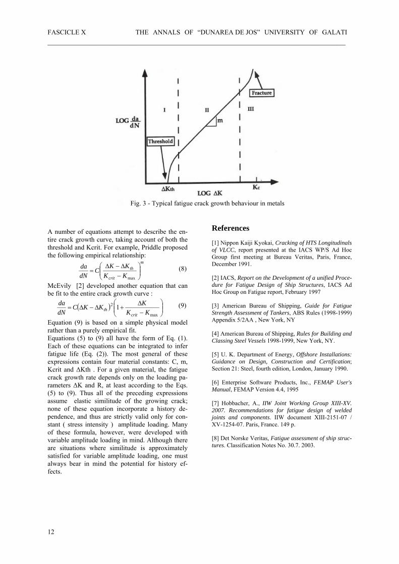
THE ANNALS OF “DUNAREA DE JOS” UNIVERSITY OF GALATI FASCICLE X ___________________________________________________________________________ m , K = Parameters of the upper segment of the S-N curve ∆m = Slope change of the upper to lowe segment of the S-N curve γ(a,x) = incomplete gamma function. Legendre form Γ(a) = Gamma function . As can be seen in Equation (1), the two parameters of the Weibull distribution used are the stress range SR at the probability of exceedance of 1/ NR, and the Weibull shape parameter ξ. For a given set of SR, ξand S-N curve, the fatigue damage (or fatigue life) can be readily obtained using the equation. Simi-larly, for a given set of ξ, S-N curve and a specified fatigue damage (or fatigue life), the stress range SR can be determined. The SafeHull assessment procedures were devel-oped from various sources including the Palmgren-Miner linear damage model, U. K. DEn’s S-N curves, environment data of the North-Atlantic Ocean, etc. In assessing the adequacy of the struc-tural configuration and the initially selected scant-lings, the fatigue strength of the hull girder and individual structural members or details is to be in compliance with the failure criteria specified. The SafeHull fatigue criteria were established to allow consideration of a broad variation of structural de-tails and arrangements so that most of the important structural details in the vessel can be assessed for their adequacy in fatigue strength. To this end, the structural response should be calculated by a finite element structural analysis as defined here or by other equivalent and effective means. Due consid-eration should be given to structural members or details expected to have high stresses. While this is a simplified analysis, some judgments are still re-quired in applying the approach to the actual de-sign. 5. Empirical Fatigue Crack Growth Equations Figure 2 is a schematic log-log plot of da/dN ver-sus ∆K, which illustrates typical fatigue crack growth behavior in metals. The sigmoidal curve contains three distinct regions. At intermediate ∆K values, the curve is linear, but the crack growth rate deviates from the linear trend at high and low ∆K levels. In the former case, the crack growth rate accelerates as Kmax approaches Kcrit the fracture toughness of the material. At the other extreme, da/dN approaches zero at a threshold ∆K; In [2], the causes of this threshold are explored. The linear region of the log-log plot in Fig. 2 can be described by a power law:
mKCdNda
∆= (3)
where C and m are material constants that are de-termined experimentally . According to Eq. (3) , the fatigue crack growth rate depends only on ∆K ; da/dN is insensitive to the R ratio in Region II . Paris and Erdogan [2] were apparently the first to discover the power law relationship for fatigue crack growth in Region II. They proposed an expo-nent of four, which was in line with their experi-mental data. Subsequent studies over the past three decades, however, have shown that m is not neces-sarily four, but ranges from two to seven for vari-ous materials . Equation (from up) has become widely known as the Paris Law. A number of researchers have developed equations that model all or part of the sigmoidal da/dN - ∆K relationship. Many of these equations are empirical, although some are based on physical considera-tions. Forman [2] proposed the following relation-ship for Regions II and ID:
( ) KKR
KCdNda
crit
m
∆−−∆
=1
(4)
This equation can be rewritten in the following form
1max
1
−
∆=
−
KK
KCdNda
crit
m (5)
Thus the crack growth rate becomes infinite as Kmax approaches Kcrit. Note that the above relationship accounts for R ratio effects, while Eq. (10.5) assumes that da/dN depends only on ∆K. Another important point is that the material constants C and m in the Forman equation do not have the same numerical values or units as in the Paris-Erdogan equation (Eq. (10.5)). Weertman [9] proposed an alternative semiempiri-cal equation for Regions II and III:
2max2
4
KKKC
dNda
crit−∆
= (6)
This equation can be made more general with a variable exponent, m on ∆K. Again, the fitting pa-rameters, C and m, do not necessarily have the same values or units in the various crack growth equations. Both the Forman and Weertman equations are as-ymptotic to Kmax = Kcrit but neither predicts a threshold. Klesnil and Lukas [4] modified Eq. (6) to account for the threshold:
)( mth
m KKCdNda
∆−∆= (7)
Donahue [2] suggested a similar equation, but with the exponent, m, applied to the quantity (∆K-∆Kth). In both cases, the threshold is a fitting pa-rameter to be determined experimentally .One problem with these equations is that ∆Kth often depends on the R ratio.
FASCICLE X THE ANNALS OF “DUNAREA DE JOS” UNIVERSITY OF GALATI __________________________________________________________________________ A number of equations attempt to describe the en-tire crack growth curve, taking account of both the threshold and Kcrit. For example, Priddle proposed the following empirical relationship:
m
crit
th
KKKK
CdNda
⎟⎟⎠
⎞⎜⎜⎝
⎛−∆−∆
=max
(8)
McEvily [2] developed another equation that can be fit to the entire crack growth curve :
( ) ⎟⎟⎠
⎞⎜⎜⎝
⎛−∆
+∆−∆=max
2 1KK
KKKCdNda
critth
(9)
Equation (9) is based on a simple physical model rather than a purely empirical fit. Equations (5) to (9) all have the form of Eq. (1). Each of these equations can be integrated to infer fatigue life (Eq. (2)). The most general of these expressions contain four material constants: C, m, Kcrit and ∆Kth . For a given material, the fatigue crack growth rate depends only on the loading pa-rameters ∆K and R, at least according to the Eqs. (5) to (9). Thus all of the preceding expressions assume elastic similitude of the growing crack; none of these equation incorporate a history de-pendence, and thus are strictly valid only for con-stant ( stress intensity ) amplitude loading. Many of these formula, however, were developed with variable amplitude loading in mind. Although there are situations where similitude is approximately satisfied for variable amplitude loading, one must always bear in mind the potential for history ef-fects.
Fig. 3 - Typical fatigue crack growth behaviour in metals
References
[1] Nippon Kaiji Kyokai, Cracking of HTS Longitudinals of VLCC, report presented at the IACS WP/S Ad Hoc Group first meeting at Bureau Veritas, Paris, France, December 1991.
[2] IACS, Report on the Development of a unified Proce-dure for Fatigue Design of Ship Structures, IACS Ad Hoc Group on Fatigue report, February 1997
[3] American Bureau of Shipping, Guide for Fatigue Strength Assessment of Tankers, ABS Rules (1998-1999) Appendix 5/2AA , New York, NY
[4] American Bureau of Shipping, Rules for Building and Classing Steel Vessels 1998-1999, New York, NY.
[5] U. K. Department of Energy, Offshore Installations: Guidance on Design, Construction and Certification; Section 21: Steel, fourth edition, London, January 1990.
[6] Enterprise Software Products, Inc., FEMAP User's Manual, FEMAP Version 4.4, 1995
[7] Hobbacher, A., IIW Joint Working Group XIII-XV. 2007. Recommendations for fatigue design of welded joints and components. IIW document XIII-2151-07 / XV-1254-07. Paris, France. 149 p.
[8] Det Norske Veritas, Fatigue assessment of ship struc-tures. Classification Notes No. 30.7. 2003.
12

THE ANNALS OF “DUNAREA DE JOS” UNIVERSITY OF GALATI FASCICLE X ___________________________________________________________________________
Lagrange Equations with Multipliers for the Rigid Body
Sorin Dumitru Muşat & Liliana Celia Rusu Dunarea de Jos University of Galati
ABSTRACT
The objective of the present paper is to establish some equations concerning the dynamics of the rigid bodies with kinematical constrains. Starting from the Lagrange equations with multipliers for the incremental motion, the differential equations with multipliers for the rigid body with kin-ematical constrains are established by imposing the limits. It is operated with the projections of the vectors velocity of translation and the angular velocities on the axis of the reference system considered linked with the rigid body (quasi velocities). The equations of the kinematical con-strains are used in a nonholonomic form. The constraining forces are resulting by projecting the forces on the axes linked with the rigid body.
1. Introduction In dynamics of the rigid body with general motion
the so called Newton-Euler([1]) equations are cur-rently used. The motion is considered decomposed in two parts: the motion of the centre of gravity and the motion of a rigid with a fixed point in the centre of gravity. The equation of motion of the gravity (New-ton) is used with thee projections of the vectors on the axes of a fix reference system. The equations of mo-tion with respect to the centre of gravity (Euler) are operating with the projections of the vectors on the axes of the reference system that is linked with the moving rigid body. In this work an approach will be presented that considers as reference an arbitrary point of the rigid body; either for the translation and the rotation part of the motion the projections of the vec-tors on the axes of the reference system that is linked with the rigid body (the quasi velocity concept being thus used). The kinematical constrains either holonomic or non holonomic are used in a non holonomic form and are introduced in the computa-tions by means of the Lagranges’ multipliers. Such an approach allows in many situations a convenient rep-resentation of the kinematical constrains and the de-termination of the constraining forces through their projections on the axes of the reference system that is linked with the rigid body.
2. Incremental motion of a free rigid body We consider ( )0 0 0 0 0, , ,O x y zℜ a fix Cartesian
reference system, ( ), , ,O x y zℜ a reference system linked with the moving rigid body and
( ), , ,O x y z∗ ∗ ∗ ∗ ∗ℜ a Cartesian reference system that
coincides with ℜ at the current time moment (fig.1). t
0rr x
y
z 0r∆r
∆Φuuur
Or∆r
A
rr
0O
0z
0y
0x
O∗
z∗
y∗
x∗
O
Figure 1
13

FASCICLE X THE ANNALS OF “DUNAREA DE JOS” UNIVERSITY OF GALATI ___________________________________________________________________________ The spatial disposal of the reference system ∗ℜ is defined by the three parameters of position,
, ,O O Ox y z∗ ∗ ∗ , and by the three orientation angles
, ,ψ θ ϕ∗ ∗ ∗ , that are included in the vector of dis-placement:
T Tt r⎡ ⎤= ⎣ ⎦x x x
T,
where: T
,t O O O rx y z ψ ϑ ϕ∗ ∗ ∗ ∗ ∗ ∗⎡ ⎤ ⎡= =⎣ ⎦ ⎣x xT⎤⎦ .
The orientation matrix of the rigid body at the mo-ment is: t
( )r=R R x . The incremental motion of the rigid body is the mo-tion from the moment to the time moment
with a finite very small. The displacement of the rigid body from the time moment to the mo-ment
tt + ∆t t∆
tt τ+ , 0 tτ≤ ≤ ∆ , is defined by the variation
of the vector and of the variation of the rota-
tion angle vector ∆Φ that measures the modification of the rigid body orientation from the moment to the time moment t
Or∆uuur
Orr
uuur
tτ+ .
The position of the reference system with re-spect with is given by the vector cu
ℜ∗ℜ t Oq r≡ ∆
uuuuurrtqr
which is very small; we make the notation:
t x y zt t t⎡ ⎤= ⎣ ⎦qT
,
Where , ,x y zt t t are the projections of the vector tqr on
the axes of the reference system . ∗ℜWe define the orientation of the reference system with respect to with the angle ; a random
orientation of the rigid body is obtained as a result of three successive rotations: along the axis O z
ℜ ∗ℜ RPY
∗ ∗ with the angle xϕ (Roll), rotation with angle yϕ along the
axes O y∗ ∗ (Pitch) and rotation with the angle
xϕ along the axis (Yaw). The orientation matrix
of the reference system with respect to
O x∗ ∗
ℜ ∗ℜ is: 1 0 00 cos sin0 sin cos
cos 0 sin cos sin 00 1 0 sin cos 0
sin 0 cos 0 0 1
x x
x x
y y z z
z z
y y
ϕ ϕϕ ϕ
ϕ ϕ ϕ ϕϕ ϕ
ϕ ϕ
⎡ ⎤⎢ ⎥= − ×⎢ ⎥⎢ ⎥⎣ ⎦
⎡ ⎤ −,
⎡ ⎤⎢ ⎥ ⎢ ⎥×⎢ ⎥ ⎢ ⎥⎢ ⎥ ⎢ ⎥− ⎣ ⎦⎣ ⎦
R
and depends of the order of the three rotations. For small values of the angles , ,x y zϕ ϕ ϕ that are specific
to the incremental motion the following approxima-
tions are admitted sinφ=φ, cosφ=1. Neglecting now the terms that are quadratic in the angles, results:
r≅ +R I q% where I is the 3 3× unit matrix and
00
0
z y
r z
y x
ϕ ϕ
xϕ ϕϕ ϕ
⎡ ⎤−⎢ ⎥= −⎢ ⎥⎢ ⎥−⎣ ⎦
q%
Is the anti symmetrical matrix associated with the vector rqr , constructed with the projections
, ,x y zϕ ϕ ϕ of the vector ∆Φuuur
on the axes of the refer-
ence system ∗ℜ . The orientation matrix no longer depends of the order of the three rotations. For the incremental matrix the orientation of the reference system
R
ℜwith respect to ∗ℜ will be specified by the vector :
r x y zϕ ϕ ϕ⎡ ⎤= ⎣ ⎦qT
. The position and orientation of the reference sys-
tem ℜwith respect to ∗ℜ will be defined by:
t r x y z x y zϕt t t ϕ ϕ⎡ ⎤ ⎡ ⎤= = ⎣⎣ ⎦q q qTT T
⎦T
.
The following notation will be also made:
t r x y z x y zt t t ϕ ϕ ϕ⎡ ⎤ ⎡ ⎤= = = ⎣ ⎦⎣ ⎦v q v v & & && & & &T TT T
. For the incremental motion the projections of any
vector on the axes of the reference system ℜ the same projections on the correspondent axes of the reference system ∗ℜ will be considered.
3. Lagrange equations for the incremental
motion of a free rigid body
The Lagrange equations for the incremental mo-tion of a rigid body (as seen by an observer linked with the reference system ∗ℜ ) are written as:
d E Edτ
∂ ∂⎛ ⎞ − =⎜ ⎟∂ ∂⎝ ⎠Q
v q
where E is the kinetic energy of the rigid, Q the vec-tor of the generalized forces (projections on the axes of the reference system ∗ℜ (or ) of the resultant and of the resultant moment with respect to O
ℜ∗ of the
forces acting on the rigid body. The velocity of a random point belonging to the
rigid body is given by: O Ov vr ru q r r q= + × = − ×
r r r r r r r
14

THE ANNALS OF “DUNAREA DE JOS” UNIVERSITY OF GALATI FASCICLE X ___________________________________________________________________________ or, in matrix form with the projections of the vectors on the axes of the reference system ℜ ,
t r= −u v r v% where is the anti symmetrical matrix associated with the vector ,
r%rr
00
0
z yz xy x
−⎡ ⎤⎢ ⎥= −⎢ ⎥⎢ ⎥−⎣ ⎦
r%
with , ,x y z the coordinates of the generic point, , in the reference system ℜ .
A
The kinetic energy of the rigid body is:
( )( ) ( )
( )( )
( )
( )
( )
( )
( )
21 12 2
12
12
12
sau
C C
t r t rC
t tC
t rC
r tC
r rC
E u dm dm
dm
dm
dm
dm
dm
= =
= − −
⎛ ⎞⎜ ⎟= −⎜ ⎟⎝ ⎠
⎛ ⎞⎜ ⎟⎜ ⎟⎝ ⎠
− +⎛ ⎞⎜ ⎟⎜ ⎟⎝ ⎠⎛ ⎞⎜ ⎟+⎜ ⎟⎝ ⎠
∫ ∫
∫
∫
∫
∫
∫
u u
v v r v rv
v r v
v r v
v r v
v r r v
r
% %
%
%
% %
T
T T T
T
T
T T
T T
=
=
where ( )C indicates the rigid body. The following compact form can be considered:
12E = v vTM
where is the generalized inertia matrix of the rigid body with respect to the reference system
, symmetrical and positively defined,
M
( , , ,O x y zℜ )
⎤⎥
O
O O
−⎡ ⎤⎢ ⎥⎣ ⎦
M SS J
M =
with: 1 0 00 1 0 ,0 0 1
00 ,
0
,
O
x xy xz
O yx y yz
zx zy z
M
J J JJ J JJ J J
ζ ηζ ξη ξ
⎡ ⎤⎢ ⎥= ⎢ ⎥⎢ ⎥⎣ ⎦−⎡ ⎤
⎢ ⎥= −⎢ ⎥⎢ ⎥−⎣ ⎦⎡ − −⎢= − −⎢ ⎥⎢ ⎥− −⎣ ⎦
M
S
J
where M is the mass of the rigid body, , ,ξ η ζ the coordinates of the center of gravity of the rigid body with respect to the reference system ℜ ,
, ,x y zJ J J , , ,xy yx yz zy zx xzJ J J J J J= = = the axial
and centrifugal inertia moments with respect to the axes and the perpendicular pair of plans of the refer-ence system ℜ .
The kinetic energy can be written as:
12
12
or+
t t
t O r
r O t
r O r
E = +
−+ +
+
v Mv
v S v
v S vv J v
T
T
T
T
The first term from the left side of the Lagrange
equations can be written:
t
r
EE
E
∂⎧ ⎫⎪ ⎪∂∂ ⎪ ⎪= ⎨ ⎬∂∂ ⎪ ⎪⎪ ⎪∂⎩ ⎭
vv
v
where:
,
.
t O rt
O t O rr
E
E
∂= −
∂∂
= +∂
Mv S vv
S v J vv
Hence the first term results:
t
r
Ed Ed E
τ
τ
τ
⎧ ⎫⎛ ⎞∂ ∂⎪ ⎪⎜ ⎟∂ ∂∂ ⎪ ⎪⎛ ⎞ ⎝ ⎠= ⎨ ⎬⎜ ⎟∂⎝ ⎠ ⎛ ⎞∂ ∂⎪ ⎪
⎜ ⎟⎪ ⎪∂ ∂⎝ ⎠⎩ ⎭
vv
v
with:
,
,
t O r r t r O tt
O t O r r O t r O rr
E
Eτ
τ
⎛ ⎞∂ ∂= − + −⎜ ⎟∂ ∂⎝ ⎠
⎛ ⎞∂ ∂= + + +⎜ ⎟∂ ∂⎝ ⎠
Mv S v v Mv v S vv
S v J v v S v v J vv
& & % %
& & % % &
where is the anti-symmetrical matrix associated with the angular velocity vector
rv%vr ω≡r r
, with the projections on the axes of the reference system ℜ . The derivation rule of the vectors defined with respect to a moving reference system ( ) was accounted for. Hence the following compact form can be written:
ℜ
Eτ
∗∂ ∂⎛ ⎞ = −⎜ ⎟∂ ∂⎝ ⎠v Q
v&M
15

FASCICLE X THE ANNALS OF “DUNAREA DE JOS” UNIVERSITY OF GALATI ___________________________________________________________________________
t
where -r r O
r O r O r
∗ ⎡ ⎤ ⎧ ⎫= − ⎨ ⎬⎢ ⎥
⎩ ⎭⎣ ⎦
v M v S vQ
v S v J v% %
% %.
The second term from the Lagrange equations is:
.E∂=
∂0
q
Let us consider ( , ,k k t tF F tτ τ )τ+ += x vr r
+ the
forces acting in the points ( ) , 1,...,k kA r k n=r
of the rigid body. For expressing the generalized forces
can be observed that the modifica-
tion of the vector in the incremental motion (by defining the displacement of the point
t r⎡= ⎣Q Q QTT T ⎤⎦
0krr
kA in the mo-
tion with respect to the reference system ∗ℜ ) can be written:
0k Or r∆ = ∆ + ∆Φ×
uuurr rkrr
r
. In matrix form with the projections of the vectors
on the axes of the reference system ℜ , can be written 0k t k∆ = −r q r q% .
The generalised forces and will be ex-
pressed as: tQ rQ
( )0
1 1
n nk
t k tk kt= =
∂ ∆= → =
∂∑ ∑r
Q F Qq
T
kF ,
( )0
1
nk
r k rk r=
∂ ∆= → =
∂∑r
Q F Qq
%
T
1
n
k kk=∑r F .
In and are the resultant force and moment of the force with respect to the reference point are included as projections on the axes of the reference system ℜ . Will be obtained in general:
tQ rQO
( ), ,t t tτ τ τ+ += +Q Q x v . Hence the equations of motion can be written in
the following form: ( ) ( ), ,t t t tτ τ τ τ∗
+ + += +v Q v Q x v&M + (1) The parameters of position for the incremental
motion are appearing explicitly in equations (1). Now considering the limits , 0t∆ → 0τ → , the equations (1) become ( ) ( ), ,t∗= +v Q v Q x v&M (2)
where and are those from the moment t . The equations (2) describe the instantaneous motion of the free body. The equations (2) were deduced from La-grange equations but they have the specitifity of Euler equations for rigid body with a fix point in the sense that that are operating with the projections of the kin-
ematical parameters of the first order (translation and angular velocities) on the axis of a reference system linked with the rigid body (quasi velocities).
x v
The following equation is added to the equation (2): ( )r=x L x v& (3) where the matrix has the structure L
( )( )
r
r
⎡ ⎤= ⎢ ⎥⎣ ⎦
R x 0L
0 R x .
The differential equations (3) allow a complete solv-ing of the problem of the motion of a free rigid body. 4. Kinematical constrains imposed to the
rigid body. Equations with multipliers
It is considered a rigid body subjected to kinema-tical constrains scleronomous, holonomic or non-holonomic, having the following nonholonomic form:
( ) =A x v 0 and that for the incremental motion can be written: ( )t tτ τ+ + =A x v 0 .
The Lagrange equations with multipliers ([2]) for the incremental motion of a rigid body can be written:
( ) ( ) ( )
( )T, ,
.t t t t
t t
tτ τ τ τ
τ τ
τ∗+ + + +
+ +
= + + +=
v Q v Q x v A x λA x v 0
&M ,
Now making 0t∆ → , 0τ → , will be obtained
( ) ( ) ( )( )
T, , ,t∗= + +=
v Q v Q x v A x λA x v 0
&M (4)
To this is added the following relationship: ( )r=x L x v& . (5) The differential algebraic system (4), (5) describes
the motion of the rigid motion in the presence of the kinematical constrains. λ is the vector of the La-grange multipliers and is the vector of the generalised forces corresponding to the reactions in-troduced by the kinematical constrains.
TcQ = A λ
For the case of the rigid with plane motion, con-sidering the plane xOy parallel with the director plane 0 0 0x O y , the vector is reduced to v
Tv v vtx ty rz ω⎡ ⎤= ≡⎣ ⎦v and equations (2) become:
0 0 v0 0 v0 0
0 v0 v
0
tx
ty
z
tx tx
ty ty
rz
MM
JM M Q
M M QM M Q
ωω ωξ
ω ωηωξ ωη ω
⎡ ⎤⎧ ⎫⎪ ⎪⎢ ⎥ =⎨ ⎬⎢ ⎥⎪ ⎪⎢ ⎥⎣ ⎦ ⎩ ⎭
− −⎡ ⎤⎧ ⎫ ⎧ ⎫⎪ ⎪ ⎪ ⎪⎢ ⎥= − − +⎨ ⎬ ⎨ ⎬⎢ ⎥⎪ ⎪ ⎪ ⎪⎢ ⎥⎣ ⎦ ⎩ ⎭ ⎩ ⎭
&
&
& (6)
16

THE ANNALS OF “DUNAREA DE JOS” UNIVERSITY OF GALATI FASCICLE X ___________________________________________________________________________
5. Examples
1. Will be considered first a rigid body with a fixed axis in the points and A B (figure 2). It is considered that the forces acting on the rigid body are reduced in O to maximum a moment having the di-rection of the rotation axis. The elements of the resul-tant will be denoted by ( ), ,0x y
rxR R R , (for the force)
and ( ), ,0O xM M y
rM , (for the moment). The dy-
namic reactions will obey the following relationships:
, ;,
x A B y A B
x A B y A B
X X Y YY a Y b X a X b= + = +
= − = − +R R
M M
The kinematical constrains imposed to the rigid
body in nonholonomic form can now be written: v v v 0, v vtx ty tz rx ry= = = = = 0
⎥⎥⎥⎥
And can be introduced in the equations from above:
1 0 0 0 00 1 0 0 00 0 1 0 0
0000
0
0 00 0
0 0 0
0 00 0
0 0 0
x xy xz
yx y yz
zzx zy
z
z
z
z
M M
J J JM J J J
J J J
M
M
⎡ ⎤−⎡ ⎤ ⎡ ⎤ ⎧ ⎫⎢ ⎢ ⎥ ⎢ ⎥ ⎪ ⎪−⎢ ⎢ ⎥ ⎢ ⎥ ⎪ ⎪⎢ ⎢ ⎥ ⎢ ⎥− − ⎪ ⎪⎣ ⎦ ⎣ ⎦ ⎪ ⎪⎢ =⎨ ⎬⎢ ⎡ ⎤− − −⎡ ⎤ ⎪ ⎪⎢ ⎢ ⎥⎢ ⎥ ⎪ ⎪− −⎢ ⎢ ⎥⎢ ⎥ ⎪ ⎪⎢ ⎢ ⎥ =⎢ ⎥− − − − ⎪ ⎪⎩ ⎭⎣ ⎦ ⎣ ⎦⎣
−⎡ ⎤⎢ ⎥⎢ ⎥⎢ ⎥⎣ ⎦= −−⎡
⎢
⎣
&
ζ ηζ ξη ξ
ζ ηζ ξ
ω ϕη ξ
ωω
ωω
00
0
0 0 0 00 0 0 0
0 0 0 0 000 000 0
0 0 0
z
z
z x xy xz
z yx y yz
zzx zy
M
J J JJ J JJ J J
⎛ ⎡⎜ ⎢⎜ ⎢⎜ ⎢⎜ ⎢⎜ −⎢ ⎤ ⎡ ⎤⎜ ⎢ ⎥ ⎢ ⎥⎜ ⎢ ⎢ ⎥ ⎢ ⎥⎜ ⎢ ⎢ ⎥ ⎢ ⎥− −⎦ ⎣ ⎦⎣⎝
⎞⎤− −⎡ ⎤ ⎡ ⎤ ⎧ ⎫⎟⎥⎢ ⎥ ⎢ ⎥ ⎪ ⎪− ⎟⎥⎢ ⎥ ⎢ ⎥ ⎪ ⎪⎟⎥⎢ ⎥ ⎢ ⎥− − ⎪ ⎪⎣ ⎦ ⎣ ⎦ ⎪ ⎪⎟⎥ ⎨ ⎬⎟⎥⎡ ⎤− − −⎡ ⎤ ⎪⎟⎥⎢ ⎥⎢ ⎥ ⎪− − ⎟⎥⎢ ⎥⎢ ⎥ ⎪⎟⎥⎢ ⎥⎢ ⎥ − − ⎪⎩⎣ ⎦ ⎣ ⎦ ⎦ ⎠
ζ ηζ ξη ξ
ω ζ ηω ζ ξ
η ξ
ωω
ω
00000
0
x
y
x
⎥⎥⎥⎥⎦
y
zM
⎧ ⎫ ⎧ ⎫⎪ ⎪ ⎪ ⎪⎪ ⎪ ⎪ ⎪⎪ ⎪ ⎪ ⎪⎪ ⎪ ⎪ ⎪+ +⎨ ⎬ ⎨ ⎬
⎪ ⎪ ⎪ ⎪ ⎪⎪ ⎪ ⎪ ⎪ ⎪⎪ ⎪ ⎪ ⎪ ⎪
⎪ ⎪⎪ ⎪ ⎪ ⎩ ⎭⎭ ⎩ ⎭
RR0
MM
Extracting the significant equations results:
2
2
2
2
,,,
,,
A B z z
A B z z
A B yz z xz z
A B xz z yz
z z z
X X M MY Y M MY a Y b J JX a X b J J
J M
ξω ηωηω ξωω ω
zω ωω
+ = −+ = +− = −
− + = − −=
&
&
&
&
&
that is the differential equation of motion and the equations for determining the dynamical reactions.
0 ,z z
yR
2. Let now be considered the well known problem of a skate sliding in the horizontal plane 0 0 0x O y (figure 3). The only force applied to the skate is the gravity force. The friction coefficient is considered zero along the skate and tends to infinity in the direction normal to the skate. The mass of the skate is M and the inertia moment with respect to the axis Oz is J . The initial conditions are define by end 0v 0ω .
The kinematical constrain (strictly nonholonomic)
results from the condition that the velocity of the con-tact point to be oriented along the axis, Ox
0 v 1 v 0 0tx ty ω⋅ + ⋅ + ⋅ = ,
that is [ ]0 1 0=A .
The equations with multipliers (6) will be written:
t yQ
ϑ v rz
v ty
v tx
0ω
0v0O
0y
0x
O
y
x
Figure 3
O
( )vrzω ϕ= = &
ϕ
ϕ xM
yM
xR
BY
BX
AY
AX
( ), ,C ξ η ζ y
x
0y
0x
B
0O O≡
A
b
a
Figure 2
17

FASCICLE X THE ANNALS OF “DUNAREA DE JOS” UNIVERSITY OF GALATI ___________________________________________________________________________
0
0 0 v0 0 v0 0
0 0 v0 0 v 1
0 0 0 0
tx
ty
tx
ty
MM
JM
M
ωω
ω λω
⎡ ⎤ ⎧ ⎫⎪ ⎪⎢ ⎥ =⎨ ⎬⎢ ⎥⎪ ⎪⎢ ⎥⎣ ⎦ ⎩ ⎭
−⎡ ⎤ ⎧ ⎫⎪ ⎪⎢ ⎥= − +⎨ ⎬⎢ ⎥⎪ ⎪⎢ ⎥⎣ ⎦ ⎩ ⎭
&
&
&
⎡ ⎤⎢ ⎥⎢ ⎥⎢ ⎥⎣ ⎦
.
(7)
The first and third equations from (7) lead to:
0
0 0
v 0 v constant= v ,0 constant= ;
tx tx
tω ω ω ϑ= → =
= → = =&
& ω
The second equation from (7) leads: 0 0v vtxM Mλ ω ω= =& & .
The force introduced by the kinematical constrains is:
TT 0 0ct yQλ ⎡ ⎤= = ⎣ ⎦Q A
where 0 0vt yQ Mλ ω= = .
The relationship (5) leads to: ( ) ( )( ) ( )
0 0 0
0 0
cos sin vsin cos 0
O
O
x t ty t t
ω ωω ω
−⎡ ⎤⎧ ⎫ ⎧ ⎫=⎨ ⎬ ⎨ ⎬⎢ ⎥
⎩ ⎭⎩ ⎭ ⎣ ⎦
&
&
That is to the following differential equations:
( )( )
0 0
0 0
v cos ,
v sin ,O
O
x t
y t
ω
ω
=
=
&
&
By integration results:
( ) ( )0 00 0
0 0
v vsin , cosO Ox t y tω ωω ω
= = − +
That represent the parametrical equations of a circle with the radius 0 0vR ω= and the center on the
axis. 0Oy
6. Conclusions
Starting from the Lagrange equations with multi-pliers for the incremental motion bay passing to the limits the differential equations with multipliers for the instantaneous motion of the rigid body with kin-ematical constrains were established. Analogue with Euler equations for the rigid body with a fixed point that operate with the projections of the angular veloc-ity vector on the axes of the reference system linked with the rigid body, the well known equations New-ton-Euler, operate with the projections of the angular velocities vectors on the axes of the reference system linked with the rigid body.
Moreover the instantaneous motion of the rigid body can be defined in any point, , belonging to the rigid body. The equations of the kinematical con-strains are used in a nonholonomic form.
O
The constraining forces are obtained also as pro-jections on the axes of the reference system linked with the rigid body.
7. References
1. HAUG, J.E., 1989, Computer aided kinematics and dynamics of mechanical systems, Allyn and Bacon.
2. LAZǍR,D., 1976, Principiile mecanicii analitice, Editura tehnică, Bucureşti
18
THE ANNALS OF “DUNAREA DE JOS” UNIVERSITY OF GALATI FASCICLE X ___________________________________________________________________________
Study of Torsion in the Systems with Ramifications for Transmitting the Rotation Motion
Sorin Dumitru Muşat & Liliana Celia Rusu
Dunarea de Jos University of Galati
ABSTRACT
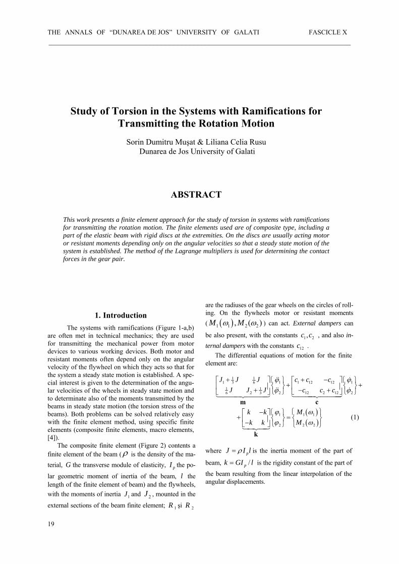
This work presents a finite element approach for the study of torsion in systems with ramifications for transmitting the rotation motion. The finite elements used are of composite type, including a part of the elastic beam with rigid discs at the extremities. On the discs are usually acting motor or resistant moments depending only on the angular velocities so that a steady state motion of the system is established. The method of the Lagrange multipliers is used for determining the contact forces in the gear pair.
1. Introduction The systems with ramifications (Figure 1-a,b)
are often met in technical mechanics; they are used for transmitting the mechanical power from motor devices to various working devices. Both motor and resistant moments often depend only on the angular velocity of the flywheel on which they acts so that for the system a steady state motion is established. A spe-cial interest is given to the determination of the angu-lar velocities of the wheels in steady state motion and to determinate also of the moments transmitted by the beams in steady state motion (the torsion stress of the beams). Both problems can be solved relatively easy with the finite element method, using specific finite elements (composite finite elements, macro elements, [4]).
The composite finite element (Figure 2) contents a finite element of the beam (ρ is the density of the ma-terial, the transverse module of elasticity, the po-
lar geometric moment of inertia of the beam, the length of the finite element of beam) and the flywheels, with the moments of inertia
G pIl
1J and , mounted in the
external sections of the beam finite element; 2J
1R şi 2R
are the radiuses of the gear wheels on the circles of roll-ing. On the flywheels motor or resistant moments ( ( )1 1 2 2, (M M )ω ω ) can act. External dampers can
be also present, with the constants , and also in-ternal dampers with the constants .
1 2,c c
12cThe differential equations of motion for the finite
element are:
( )( )
1 11 1 1 12 12 13 6
1 12 2 12 2 12 26 3
1 11
2 22
(1)
J J J c c cJ J J c c c
Mk kMk k
ϕ ϕϕ ϕ
ωϕωϕ
+ + −⎡ ⎤⎧ ⎫ ⎡ ⎤ ⎧ ⎫+ +⎨ ⎬ ⎨⎢ ⎥ ⎢ ⎥+ − +⎩ ⎭ ⎣ ⎦ ⎩ ⎭⎣ ⎦
⎧ ⎫− ⎧ ⎫⎡ ⎤+ =⎨ ⎬ ⎨ ⎬⎢ ⎥−⎣ ⎦ ⎩ ⎭ ⎩ ⎭
cm
k
&& &
&& &144424443144424443
14243
⎬
where pJ I lρ= is the inertia moment of the part of
beam, /pk GI l= is the rigidity constant of the part of
the beam resulting from the linear interpolation of the angular displacements.
19

FASCICLE X THE ANNALS OF “DUNAREA DE JOS” UNIVERSITY OF GALATI ___________________________________________________________________________
2. The equations of motions for the system without kinematical constrains
The gear pairs achieves kinematical constrains (the relative motion of the gearing wheels is rolling without sliding at the level of the rolling circles) so that at the level of the system some angular displacements are independent while some others are dependent. It is thus made a numbering of the displacement on the system by numbering first the independent displacements and after this the dependent displacements (Figure 1-a,b). The numbers in the brackets correspond to the numbers of the finite elements.
The kinematical constrains are considered un-bounded and the matrices of this system ob-tained by assembling the matrices of the finite elements were thus built.
, ,M C Km,c,k
The assembling operation means including the ele-ments of the elementary matrices ( )e m,c,k inside the correspondent matrices of the system without con-strains ( ), ,S M C K (Figure 3) (see for example also [3]). The correspondence matrix , between the numbers of the displacements from the numbering on the system and the numbering of the displacements on the element (Figure 3a). The line ne from is ana-lysed, this corresponds to the finite element with the number
MC
MC
( )ne . An element from this line is thus con-sidered. The number of the column where the element is retrieved is i . The value of this element is
1 ( , )i MC ne i= . Maintaining constant the values and i the line is again followed considering all the
elements of the line. ne
Let us consider the number of the column in which sch an element is encountered, its value being
j
1 ( , )j MC ne j= . The value is added to
the corresponding matrix of the system, by summing with the previously added elements,
( ),ne
e i⎛ ⎞⎜ ⎟⎝ ⎠ j
1 1( , )S i j
( ) ( )1 1 1 1( , ) ( , ) ,neS i j S i j e i j= + The differential equations of motion f the system
without kinematical constrains are obtained in the fol-lowing form
( )Mx x Kx F x&& & &+ C + = (2)
8ϕ
Constrain
ϕ+
ϕ+
ϕ+
1ϕ
7ϕ
.b
Figure 1
7ϕ 2ϕ
( )3 ( )1
( )2
( )n=4 8ϕ
6ϕ
5ϕ
4ϕ
3ϕ
1ϕ
.a
7ϕ 2ϕ
( )1
( )26ϕ
4ϕ
3ϕ
( )3
( )n=4
5ϕ
2c
Figure 2
12c
1c 2c
( )2 2M ω
2R
2ϕ
( )1 1M ω
ρ , , pG I
Finite element
2J 1J
1ϕ
1R
l
20

THE ANNALS OF “DUNAREA DE JOS” UNIVERSITY OF GALATI FASCICLE X ___________________________________________________________________________
3. The equations of motion for the system
with kinematical constrains The vector of the generalised displacements (rota-
tions) for the system without kinematical constrains, x , contents the nodal displacements of the system in the
form forma TT T⎡⎣x x x%= ⎤⎦ where includes the
independent displacements and
x%x includes the de-
pendent displacements. The vector of the forces and moments is obtained by localising the external mo-ments corresponding to the numbering in the system of the displacements of the wheels.
F
The equations of the kinematical constrains were obtained by expressing of the conditions of rolling without sliding between the wheels of the gearing.
0i i j jR sRϕ ϕ+ = (3’)
where iϕ is the independent displacement and jϕ is
the dependent displacement; through (sign) it is accounted for the sign convention considered (Figure 1-a,b). Thus for the cylindrical gearings for the external gearing and
s
1s = +1s = − for the internal gear-
ing.
If the beam between two wheels is long and/or has
a variable section being divided in more finite elements the equations of the kinematical constrains result from the conditions of continuity of the displacements (the equality of the rotations) in the nodal common sections
0i jϕ ϕ− = (3’’)
The kinematical constrains (3’) and (3’’) can be written in the following compact form: ( )A x A x&= 0 = 0 (4 ) The matrix is of maximum degree having the structure from Figure 4; the number of rows is equal with the number of the equations corresponding to the kinematical constrains while the number of columns is equal with the number of the displacements either independent or dependent.
A
Denoting with the number of the finite ele-ments, the total number of displacements rota-tions and with the number of the kinematical constrains (gearings), the number of the degrees of freedom the system is .
nN=2n
Nc
N=N-Nc%
The motion of the system in the presence of the kinematical constrains is described by the following system of differential algebraic equations:
c.
5 8
3 6
21
1j The matrices of the system
1i
i
j
( )ne
e i ,⎛ ⎞⎜ ⎟⎝ ⎠ j ( )1 1S i , j
M
Number of displacement on element
1j 1 i ( )ne
Number of element ↓
1
( )1
( )2
( )n
2
j i
a .
MC
b .
Figure 3
Number of equa-tion on element
The matrices of the elements
Dependent displacements
Independent displacements
continuity j i
Gearing
1− 1 000 0 0 000
M
00 jsR
AA%
=A
i j
000 iR 0 0 00 M
M
Figure 4
21

FASCICLE X THE ANNALS OF “DUNAREA DE JOS” UNIVERSITY OF GALATI ___________________________________________________________________________
c cN
( ) T ,⎫+ ⎪⎬⎪⎭
Mx x Kx F x A λA x
&& & &+ C + == 0 ,
(5)
where is the vector corresponding to the Lagrange multipliers.
λ
The differential equations of motion of the system with constrains can be obtained only in independent displacements (generalised coordinates in the real system) by eliminating the Lagrange multipliers by using the orthogonal complement matrix:
1−
⎡ ⎤= ⎢ ⎥−⎣ ⎦
IB
A A% .
The displacements were expressed as functions of the independent displacements:
x
(6) x Bx%=
By introducing equation (6) in (5) the equation of the kinematical constrains is identically verified. By multiplying the first equation in (5) with will be obtained the differential equations of the real system:
TB
( )Mx x Kx F x%&& & &% % %% % % %+ C + = (7)
where
( ) ( )T T T T, , ,= = = =M B MB C B CB K B KB F x B F x% &% % % % &
The equations (7) are solved using a numerical proce-dure. The rotations of all the wheels result from the transformation (6).
4. Lagrange multipliers – contact forces
In the steady state motion ; from the first
equation (5) results: =x 0&&
( ) T
r r r +x Kx F x A λ& &C + = (8) Now multiplying with the first equation from
(5); the matrix is a square matrix (with the di-
mensions
ATA A
N × ) and can be inversed so that:
( ) ( )( )1T −= −r rλ A A F x Cx Kx& & − r
where correspond to a random moment of the steady state motion.
rx
If an equation with the constrain corresponds to a gearing (condition of rolling without sliding on the rolling circles) the Lagrange multipliers
k
kλ represent
the magnitude of the tangential forces – Figure 5; the forces at the contact of the teeth can be thus deter-mined, N cok k sλ α= , where α is the gearing angle. If the equation for a kin-ematical constrain correspond to a continuity condition, the multiplier represents the elastic moment transmitted by the section.
For the evaluation of the maximum dynamical mo-ments from the parts of beam included in the finite ele-ments each line is selected (finite element) from the matrix by identifying the numbers and of the angles from the extremities 1 and 2 of the elements:
MC 1i 1j
1 1( ,1) , ( ,2)i ne j ne= =MC MC with which are extracted the values of the angles at the extremities, ( ) ( )1 1 2,i iϕ ϕ= =x x 2
The value of the relative rotation angle of the ex-treme sections of finite element is: 12 2 1ϕ ϕ ϕ= − , While the maximum value of the moment transmitted by the part of the beam is: 12 element 12pM GI ϕ−= ,
with which the tangential tensions necessary in the veri-fication of the resistance of the beam (statically stress) are evaluated.
5. References 1.BLAJER, W., 1992, A Projection Method Approach to Con-
strained Dynamic Analysis, ASME Journal of Applied Me-chanics , Vol. 59, pp.643-649.
2.BLAJER W., BESTLE D. and SCHIEHLEN, W. , 1994 , An Orthogonal Complement Matrix Formulation for Constrained Multibody Systems, ASME Journal of Mechanical Design , Vol.116, pp.423-428.
3.STOICESCU,L.,MODIGA,M., 1973, Metode matriceale în teoria structurilor de nave, Institutul politehnic Galaţi.
4.WU, J.-S., and CHEN, C.-H., 2001, Torsional Vibration Analy-sis of Gear-Branched Systems by Finite Element Method, Jour-nal of Sound and Vibrations, Vol.240, No.1, pp.159-182.
α
Figure 5
jR
iR kN
kN
kλ
α
kλ
22
THE ANNALS OF “DUNAREA DE JOS” UNIVERSITY OF GALATI FASCICLE X APPLIED MECHANICS, ISSN 1221-4612
2007
On the Performances of the Third Generation Spectral Wave Models in the Black Sea
Liliana Celia Rusu Dunarea de Jos University of Galati
Sonia Ponce de León Álvarez Tecnocean Ing., Barcelona, Spain
ABSTRACT
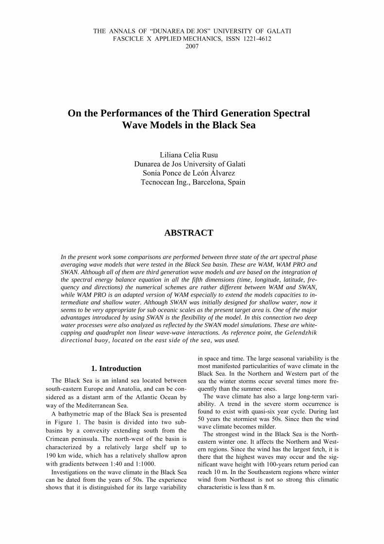
In the present work some comparisons are performed between three state of the art spectral phase averaging wave models that were tested in the Black Sea basin. These are WAM, WAM PRO and SWAN. Although all of them are third generation wave models and are based on the integration of the spectral energy balance equation in all the fifth dimensions (time, longitude, latitude, fre-quency and directions) the numerical schemes are rather different between WAM and SWAN, while WAM PRO is an adapted version of WAM especially to extend the models capacities to in-termediate and shallow water. Although SWAN was initially designed for shallow water, now it seems to be very appropriate for sub oceanic scales as the present target area is. One of the major advantages introduced by using SWAN is the flexibility of the model. In this connection two deep water processes were also analyzed as reflected by the SWAN model simulations. These are white-capping and quadruplet non linear wave-wave interactions. As reference point, the Gelendzhik directional buoy, located on the east side of the sea, was used.
1. Introduction The Black Sea is an inland sea located between
south-eastern Europe and Anatolia, and can be con-sidered as a distant arm of the Atlantic Ocean by way of the Mediterranean Sea.
A bathymetric map of the Black Sea is presented in Figure 1. The basin is divided into two sub-basins by a convexity extending south from the Crimean peninsula. The north-west of the basin is characterized by a relatively large shelf up to 190 km wide, which has a relatively shallow apron with gradients between 1:40 and 1:1000.
Investigations on the wave climate in the Black Sea can be dated from the years of 50s. The experience shows that it is distinguished for its large variability
in space and time. The large seasonal variability is the most manifested particularities of wave climate in the Black Sea. In the Northern and Western part of the sea the winter storms occur several times more fre-quently than the summer ones.
The wave climate has also a large long-term vari-ability. A trend in the severe storm occurrence is found to exist with quasi-six year cycle. During last 50 years the stormiest was 50s. Since then the wind wave climate becomes milder.
The strongest wind in the Black Sea is the North-eastern winter one. It affects the Northern and West-ern regions. Since the wind has the largest fetch, it is there that the highest waves may occur and the sig-nificant wave height with 100-years return period can reach 10 m. In the Southeastern regions where winter wind from Northeast is not so strong this climatic characteristic is less than 8 m.

FASCICLE X THE ANNALS OF “DUNAREA DE JOS” UNIVERSITY OF GALATI ___________________________________________________________________________
in aciattionby ibounificpenlots
widgooHowcomthathighthe Seawith
Figure 1: Bathymetric map of the Black Sea basin and the location of the reference point (Gelendzihik buoy, 37.98E, 44.51N)
Strong wind and large waves may also take place utumn during so-called extraordinary storms asso-ed with Mediterranean depressions. The investiga-s show that development of these storms is caused nteraction between wind waves and air flow in the ndary layer (Janssen et al., 1989). They have sig-ant destructive power. The most severed hap-
ed in 1854 and 1992, both in November, causing of damages and casualties. Second generation wave models have been
ely used in the Black Sea and they often provided d results some of them being still operational. ever, third generation models include a more plete description of the physical processes and is why their reliability is usually considerably er. During the time, various implementations of WAM model have been carried out in the Black area and their calibrations have been made either in situ or remotely sensed data.
The implementation of Vlachev et al. (2004) is
considered here as a reference because the availability of the same wind field allows a parallel on the per-formances of the two model systems developed using WAM, WAM PRO and SWAN, respectively.
2. The theoretical framework of the third generation spectral wave models
2.1 Propagation equation
Third generation wave models solve the energy bal-ance equation (1) that describes the evolution of the wave spectrum in time, geographical and spectral spaces (the spectral space is usually defined by the relative radian frequency σ and the wave direc-tionθ ):
.SDtDE
= (1)

THE ANNALS OF “DUNAREA DE JOS” UNIVERSITY OF GALATI FASCICLE X ___________________________________________________________________________ Nevertheless, while the standard WAM model con-siders the energy density spectrum (E), in SWAN the action density spectrum (N) is preferred. This is be-cause in the presence of currents action density is conserved whereas energy density is not. The action density is equal to the energy density (E) divided by the relative frequency (σ ). For large scale applica-tions this equation is related to the spherical coordi-nates defined by longitude λ and latitude φ, (Booij et al., 1999):
.
coscos
1
σθ
θσ
σ
φφφφ
λλ
SNN
NNtN
=∂∂
+∂∂
+
+∂∂
+∂∂
+∂∂
&&
&&
(2)
In the right hand side of the action balance equation
is the source (S) expressed in terms of energy density. In deep water, three components are significant in the expression of the total source term. They correspond to the atmospheric input (Sin), whitecapping dissipa-tion (Sdis) and nonlinear quadruplet interactions (Snl), respectively. Besides these three terms, in shallow water additional source terms, induced by the finite depth effects (Sfd), may play an important role and they correspond to phenomena like bottom friction, depth induced wave breaking and triad non linear wave-wave interactions. Hence the total source be-comes:
.fdnldisintotal SSSSS +++= (3)
Since shallow water processes are beyond the scope of the present work only the options available in SWAN for deep water wave modelling will be dis-cussed in the next subsections. 2.2 Standard formulations for atmospheric input and whitecapping dissipation
Transfer of wind energy to the waves is described in the third generation wave models presently operating (including SWAN) with the resonance mechanism of Phillips (1957) and the feed-back mechanism of Miles (1957). The corresponding source term that joins these two mechanisms is commonly described as the sum of the linear and the exponential growths:
( ) ( ),,, θσθσ BEASin += (4)
in which A describes the linear growth and BE the exponential growth. The expression for the term A is due to Cavaleri and Malanotte-Rizzoli (1981), with a filter to avoid growth at frequencies lower than the Pierson-Moskowitz frequency (Tolman, 1992). Two optional expressions for the coefficient B are used in the model. The first is taken from an early version of
the WAM model, known as WAM Cycle 3, (the WAMDI group, 1988). It is due to Snyder et al. (1981), rescaled in terms of friction velocity by Ko-men et al. (1984), and it is currently called the Komen parameterization. The second expression is due to Janssen (1989, 1991) and it is based on the quasi-linear wind-wave theory. Whitecapping is primarily controlled by the steepness of the waves. In the third generation wave models presently operating (including SWAN) the whitecap-ping formulations are based on the pulse model of Hasselmann (1974), as adapted by the WAMDI group (1988), so as to be applicable in finite water depth. This expression is:
( ) ( ,,~~,, θσσθσ EkkS wds Γ−= ) (5)
where σ~ and k~
denote the mean frequency and the mean wave number, and the coefficient depends on the overall wave steepness:
Γ
( ) ,~~
~1p
PMdsKJ S
SkkC ⎟⎟
⎠
⎞⎜⎜⎝
⎛⎟⎠⎞
⎜⎝⎛ +−=Γ=Γ δδ (6)
For δ=0 the expression of Γ reduces to the expression as used by the WAMDI group (1988). The coeffi-
cients Cds, δ and p are tuneable coefficients, is the
overall wave steepness and
S~
PMS~ is the value of this parameter for the Pierson-Moskowitz spectrum, (3.02×10⁻³)1/2. The values of the tunable coefficients Cds, δ and p in the SWAN model have been obtained by Komen et al. (1984) and Janssen (1992) by closing the energy balance of the waves in idealized wave growth conditions (both for growing and fully devel-oped wind seas) for deep water. This implies that co-efficients in the steepness dependent coefficient Γ depend on the wind input formulation that is used. Since two different wind input formulations are used in the SWAN model, two sets of coefficients are used. For the Komen parameterization, corresponding also to WAM Cycle 3, Cds = 2.36×10⁻⁵, δ=0 and p = 4. The tuneable coefficients are in this case Cds and
2~PMS . In the Janssen parameterization, also used in
WAM cycle 4, it is assumed again p = 4 and the tun-ing parameters used in this case are δ (default 0.5) and Cds1 (default 4.5) which is given by:
.~1
4
1 ⎟⎟⎠
⎞⎜⎜⎝
⎛=
PMdsds S
CC (7)
2.3 Alternative formulations for atmospheric input and whitecapping dissipation
A first alternative formulation for whitecapping is based on the Cumulative Steepness Method (CSM),

FASCICLE X THE ANNALS OF “DUNAREA DE JOS” UNIVERSITY OF GALATI ___________________________________________________________________________ as described in Van Vledder and Hurdle (2002). With this method, dissipation due to whitecapping depends on the steepness of the wave spectrum at and below a particular frequency. Thus the following quantity (di-rectionally dependent) is defined:
( ) ( ) ( ) .,'cos,0
2
0
2 θσθσθθθσσ π
ddEkSm
st ∫ ∫ −=
(8)
In this expression the coefficient m controls the direc-tional dependence. It is expected that this coefficient will be about 1 if the straining mechanism is domi-nant, while m is more than 10 if other mechanism play a role (e.g. instability that occurs when vertical acceleration in the waves becomes greater than grav-ity). Default in SWAN is m = 2. Hence, in this alter-native formulation the new source term for whitecap-ping dissipation is given by:
( ) ( ) ( ),,,, θσθσθσ ESCS ststwc
stwc −= (9)
with a tuneable coefficient (with the default value 0.5).
stwcC
In the last SWAN version (40.51), a second al-ternative formulation for whitecapping dissipation has been introduced. This is due to Van der Westhuysen et al. (2007), and is an adapted form of the expression of Alves and Banner (2003), which is based on the apparent relationship between wave groups and whitecapping dissipation. This adaptation seems to be more appropriate for mixed sea-swell conditions and in shallow water and it was done by removing the dependencies on mean spectral steepness and wave number in the original expression, and by applying source term scaling arguments for its calibration. This led to the following expression for the source term corresponding to whitecapping dissipation:
( ) ( )
( )( )( ) ( ),,tanh
,
42
2
θσ
θσ
Egkkh
BkBCS
op
p
rwcdsw
−⋅
⋅⎟⎟⎠
⎞⎜⎜⎝
⎛−=
(10)
in which Cds is the tunable coefficient (the default value in SWAN for this formulation is Cds = 5.0×10⁻⁵) and the density function B(k) is the azimuthal-integrated spectral saturation, which is positively cor-related with the probability of wave group-induced breaking. It is calculated in the frequency space as follows:
( ) ( ) ,,2
0
3 θθσπ
dEkckB g∫= (11)
and Br is a threshold saturation level (default value in SWAN Br=1.75×10⁻³). When B(k)>Br, waves break and the exponent p is set equal to a calibration pa-
rameter po. For B(k)≤Br there is no breaking, but some residual dissipation proved necessary. This is obtained by setting p=0. A smooth transition between these two situations is achieved in the following ex-pression deduced by Alves and Banner (2003):
( ) .110tanh22 ⎥
⎥⎦
⎤
⎢⎢⎣
⎡⎟⎟⎠
⎞⎜⎜⎝
⎛−+=
r
oo
BkBpp
p
(12) The wind input formulation used in saturation-based model is based on that by Yan (1987). This expres-sion embodies experimental findings that for strong wind forcing, 1.0* >cu (where is the friction velocity of wind and c the wave phase velocity), that is the wind-induced growth rate of waves depends quadratic on
∗u
cu∗ whereas for weaker forcing
1.0* <cu , that is the growth rate depends linearly
on cu∗ (Snyder et al, 1981):
( ) ( )
( ) ,1cos2825.0,0max
,1,
*⎥⎦
⎤⎢⎣
⎡⎟⎠⎞
⎜⎝⎛ −−=
==
αθρρ
θσσ
θσβ
cu
SE
w
a
inSnyder
(13) where aρ and wρ are the densities of air and water, respectively and α is the wind direction. Yan (1987) proposes an analytical fit through the two ranges of the form:
( )
( ) ( ) ,coscos
cos2
HFc
uE
cu
Dfit
+−+−⎟⎠⎞
⎜⎝⎛+
+−⎟⎠⎞
⎜⎝⎛=
∗
∗
αθαθ
αθβ
(14) where D, E, F and H are coefficients of the fit. Yan proposes the parameter values
,1011.3;105.5
;1044.5;100.445
32
−−
−−
×−=×=
×=×=
HF
ED (15)
which produces a reasonable fit between the curves of Snyder et al. (1981). However, Yan's fit yields a smaller growth rate than the expression of Snyder et al. (1981) for mature waves (for cu∗ lower than 0.054). Yan (1987) confirms that this leads to an un-derestimation of the evolution of mature waves com-pared to that produced using Snyder et al.'s expres-sion. Therefore in SWAN equation (14) was refitted

THE ANNALS OF “DUNAREA DE JOS” UNIVERSITY OF GALATI FASCICLE X ___________________________________________________________________________ in order to better match Snyder et al.'s expression (13) for mature waves. This yielded parameter values of:
,1002.3;102.5;1052.5;100.4
45
32
−−
−−
×−=×=
×=×=
HFED
(16)
Finally, the choice of the exponent po in equations (10) and (12) is made by requiring that the source terms of whitecapping (10) and wind input (14) have equal scaling in frequency, after Resio et al (2004). This leads to a value of po = 4 for strong wind forcing ( 1.0* >cu ) and po = 2 for weaker forcing
( 1.0* <cu ). A smooth transition between these
two limits, centered around 1.0* =cu , is achieved by the expression:
,1.0tanh3 **⎥⎦
⎤⎢⎣
⎡⎟⎠⎞
⎜⎝⎛ −+=⎟
⎠⎞
⎜⎝⎛
cu
wcu
po (17)
where w is a scaling parameter for which a value of w = 26 is used in SWAN. In shallow water, under strong wind forcing (po = 4), this scaling condition requires the additional dimensionless factor
( ) ,tanh 21−kh in equation. (10), where h is the water depth and k the wave number.
2.4 Quadruplet non linear interactions
In deep water quadruplet wave-wave interactions dominate the evolution of the spectrum. They transfer wave energy from the spectral peak both to lower frequencies, thus moving the peak frequency to lower values, and to higher frequencies, where the energy is dissipated by whitecapping. Hasselmann (1962) de-rived the transfer rate to, and from, a spectral compo-nent arising from interactions with sets of three other spectral components. The resulting source term takes the form of an integral over the phase space of inter-acting quadruplets called the Boltzmann integral:
( ) ( )
( ) ( )[( ) (
321
43214321
21434321
432144,4 ,,,.......
kdkdkd
kkkk
NNNNNNNN
kkkkGkSnl
rrr
rrrr]
)
rrrrr
⋅
−−+−−+⋅
⋅+−+⋅
⋅= ∫ ∫∞
ωωωωδδ
ω
(18) In the above relationship ω is the absolute radian frequency that equals the sum of the relative radian frequency σ and the multiplication of the wave num-ber and ambient current velocity vectors:
,uk rr⋅+= σω (19)
which is the usual Doppler shift. ( )tkNi ,,,r
φλ is the
action density for the wave number vector ikr
.
( )4321 ,,, kkkkGrrrr
is the interaction coefficient de-rived by Hasselmann (1962). The Dirac delta func-tions (δ ) in equations (18) select the resonance con-ditions, which are associated with conservation of energy and momentum in the interaction, (Hassel-mann, 1963). The source term is evaluated for
infinite water depth and then adjusted for finite depth by an empirical scaling (Herterich and Hasselmann, 1980; Hasselmann and Hasselmann, 1981).
∞,4nlS
( ) ,,44 ∞= nlpnl SdkRS (20)
( ) ( )⎪⎪
⎩
⎪⎪
⎨
⎧
≥⎥⎥⎦
⎤
⎢⎢⎣
⎡−⎟⎟
⎠
⎞⎜⎜⎝
⎛−+
<
=
5.0
25.1exp6
515.51
5.0,43.4
dk
dkdk
dk
dk
dkR
p
pp
p
p
p
(21) A full computation of the Boltzmann integral express-ing this type of non linear interactions is extremely time consuming and not convenient in any operational wave model. Nevertheless, the current version of SWAN has two methods to compute the Boltzmann integral in an exact manner, leading to four different options. The first approach is the so-called FD-RIAM technique as proposed by Hashimoto et al. (1998) and the second approach is the exact method developed by Webb, Tracy and Resio (WRT), (Resio et al., 2001) denoted in SWAN as XNL that can be acti-vated in three different modes (deep water transfer, deep water transfer with WAM depth scaling and finite depth transfer).
To reduce the computational demands involved in implementing the source term described by equa-tion (18) in SWAN, as in WAM, a discrete interaction approximation (DIA), (Hasselmann et al., 1985) is applied, in which only two quadruplets are summed. These both have the same set of frequencies:
.,75.0,25.1 4321 σσσσσσσ ==== (22) In both quadruplets, the third and fourth wave vectors coincide, while the others lie at angles °−= 5.111θ
and °= 6.332θ to this common direction.

FASCICLE X THE ANNALS OF “DUNAREA DE JOS” UNIVERSITY OF GALATI ___________________________________________________________________________
despclprfeinthplpetrcoitin
Fabcsd
This DIA has been found to be quite successful in scribing the essential features of a developing wave ectrum using the fact that the interactions between osely neighboring wave numbers reproduce the incipal features of the nonlinear transfer. Four dif-rent numerical procedures for DIA can be activated to the SWAN model: semi-implicit computation of e nonlinear transfer with DIA per sweep, fully ex-icit computation of the nonlinear transfer with DIA r sweep, fully explicit computation of the nonlinear
ansfer with DIA per iteration and fully explicit mputation of the nonlinear transfer with DIA per
eration, but neighboring interactions are interpolated a piecewise constant manner.
igure 2: Comparisons WAMC4-WAM PRO versus the Gelendzihik buoy ) Significant wave heights for the time interval November - December 1996; ) Significant wave heights for the time interval January – 6th of February 1997; ) Impact of the time step on the significant wave height results in WAM PRO (15 minutes and 5 minutes, re-p ctively); e) Wave period (Tm02), WAM PRO versus Gelendzihik, for the time interval November - December 1996;
Various options and source term parameterizations were tested for the Black Sea’s specific conditions and some results will be discussed in the next sec-tions.
3. WAM PRO versus WAM
The WAM-PRO model is the original code of the WAM cycle 4 model, which was adapted for shallow waters and high spatial applications in the PROMISE project Monbaliu et al (2000). Two aspects were consid-ered for the improvements in WAM-PRO: computational efficiency and the representation of the physical proc-esses involved in the evolution of waves in shallow wa-ter areas. As results were implemented, additional source

THE ANNALS OF “DUNAREA DE JOS” UNIVERSITY OF GALATI FASCICLE X ___________________________________________________________________________ terms were found which deal with the shallow water physics; a depth-induced wave breaking expression and six new bottom friction formulations, two of them taking into account wavecurrent interaction, have been imple-mented (Monbaliu et al 2000), a new fetch growth lim-iter (Luo and Sclavo 1997). Later a numerical improve-ment was introduced in the WAM-PRO for the nested run procedure as well as for the generation of boundary conditions for avoiding the use of a large amount of disk space (Osuna 2002).
Simulations with the WAM PRO model where performed and the results were compared with those provided by the WAM model for the same time in-terval at the end of 1996 and the beginning of 1997 (from 1st of November 1996 till 6th of February 1997) that used exactly the same wind data field, Vlachev et al. (2004). The results of the compari-sons are presented in Figure 2. As check point the Gelendzhik directional buoy located on the east coast of the sea was used.
4. SWAN versus WAM
For the same period (1st of November 1996, 6th of February 1997) SWAN model simulations were also performed. Both parameterizations Komen corresponding to WAM cycle 3 and Janssen corresponding to WAM cycle 4 were used. The direct comparisons are presented in Figures 3 and 4 while the corresponding statistical results in Table 1. As can be seen Komen parameterization gives sensible better results than Janssesn.
The results were also compared with those pro-
vided by the WAM model for the same time interval at the end of 1996 and the beginning of 1997 (TI-1) that used exactly the same wind data field, Vlachev et al. (2004). Looking at the values of the statistical pa-rameters it has to be noticed that, probably due to the better flexibility in tuning the parameters, the SWAN results are considerably better to those provided by WAM for any of the whitecapping parameterization considered. Thus, the biases obtained for the same time interval were for Hs: 0.27, for Tp: 0.43 and for Dir: 33.1. Referring to the RMSE the values obtained were for Hs: 0.53, for Tp: 1.74 and for Dir: 92.7,
which means considerably higher root mean square errors at least as regards the significant wave height and the mean direction. The scatter indices obtained were: 0.68 for Hs, 0.34 for Tp and 0.46 for Dir, which means also that the results of SWAN are better. Fi-nally the computed correlation coefficients were for Hs: 0.73, for Tp: 0.55 and 0.36 for Dir. This means also better correlations with the measured data as concerns the SWAN results.
Figure 3 Comparison Gelendzihik buoy – SWAN (Komen parameterization), Hs, Tp and Mean direction (1996.11.01h00-1997.02.06h00– 660 valid data points).
Table 1
n=684
Bias
RMSE
SI
r
Hs (m) -0.01 0.365 0.36 0.89 K Tm (s) 0.56 0.893 0.22 0.79 O Tp (s) 0.44 1.486 0.26 0.64 M Dir (°) 10.6 53.22 0.26 0.45 Hs (m) -0.04 0.469 0.47 0.81 J Tm (s) -0.06 0.855 0.22 0.70 N Tp (s) 0.04 1.59 0.28 0.52 S Dir (°) -9.57 68.60 0.32 0.32
Figure 4 Comparison Gelendzihik buoy – SWAN (Jansen parameterization), Hs, Tp and Mean direction (1996.11.01h00-1997.02.06h00– 660 valid data points).

FASCICLE X THE ANNALS OF “DUNAREA DE JOS” UNIVERSITY OF GALATI ___________________________________________________________________________
terization Q2 appears most effective from computa-2
Table4. Testing various options for quadruplets in SWAN
Another series of simulations was focused on the analysis of the influences of the quadruplet non linear interactions making a balance between the computa-tional time and the accuracy of the results. The quad-ruplet nonlinear interaction source term based on the Boltzmann integral and the DIA approach for simpli-fying the computations were described in the previous section. Thus, nine parameterizations are available in the SWAN model to account for the quadruplet inter-actions. Four of them are based on the fully computa-tion of the Boltzmann integral (FD-RIAM, XNL for deep water transfer, XNL for deep water transfer with WAM depth scaling and XNL for finite depth trans-fer), but none of these formulations can be used on a PC platform and even for workstations they cannot be yet used operationally. The fifth option available, multiple DIA, requires also a high computational ef-fort although lower than the previous cases. The ef-fectiveness of the other four different formulations that are based on the DIA approximation was as-sessed. These are: Q1- semi-implicit computation of the nonlinear transfer with DIA per sweep, Q2- fully explicit computation of the nonlinear transfer with DIA per sweep (default in SWAN), Q3- fully explicit computation of the nonlinear transfer with DIA per iteration and Q8 - fully explicit computation of the nonlinear transfer with DIA per iteration, but neighboring interactions are interpolated in piecewise constant manner. The computations were performed on a common Pentium IV PC platform with a 3.2 GHz processor and RAM memory of 1024 MB, while the time interval considered was the final part of the time interval considered in the previous simulations, only for the year 1997 (1997/01/01 -1997/02/06). The statistical results and the corresponding computer times are presented in Table 2. The default parame-
tional point of view and, for this reason, although the results when using Q1 are slightly better in all pa-rameters, the fully explicit computation of the nonlinear transfer with DIA per sweep (Q2) was preferred in further computations. In addition, the option Q4, corresponding to the multiple DIA ap-proach, was also evaluated but the computer time required was about 3 times greater than for Q2 for the time interval considered. Nevertheless, this mul-tiple DIA improve slightly the results and using it might be an option for the situations when the com-putational time is not strictly limited or when devel-oping parallel computations.
5. Final considerations Differences between wave model simulations and
measurements can be generated due to various fac-tors, most frequent being: differences between wind fields used for calculations from the real, errors due to the choices of some parameters in the wave model, model limitations in relationship with some complex physical processes and inaccurate measurements. As the present work fully illustrates, the default options, without taking into account the specific features and conditions of a specific location, are not always the most appropriate way to use a third generation wave model. Moreover, even in the same computational domain different dynamics request sometimes differ-ent settings for the wave model.
Lopatoukhin et al. (2004) provided some interest-ing information concerning the wind and wave cli-mate of the seas around Russia including the Caspian and Black Seas. Hence as regards the NCEP reanaly-sis wind the best correspondence is encountered in the North (Barents Sea where the correlation was of about 0.9). This correlation decreases when moving to the south.
As regards the comparison between the three dif-ferent third generation wave models performed here-with, the results clearly showed that SWAN might be very effective at these sub oceanic scales as the Black Sea is. The present SWAN model implementation in the Black Sea brings the main advantage of the model flexibility in tuning parameters and physical processes for a better calibration of the model in a specific site. From this point of view SWAN seems to be more appropriate for such a sub oceanic domain than WAM or even WAM PRO that are considered more tradi-tionally as generation wave models. Probably moti-vated by the same reasons, several SWAN implemen-tations are currently tested also for the entire Mediter-ranean Sea basin.
Especially in such inland seas, as the Black Sea is, most of the processes related with wave generation and deep water dissipations are sometimes rather dif-ferent than in open ocean and, although the same mathematical formulations describing these processes
n=684
Bias
RMSE
SI
r Case/Time
Hs(m) 0.01 0.32 0.29 0.92 Q1 Tp (s) 0.467 1.37 0.23 0.72 21h09min Dir(°) 20.36 51.65 0.22 0.58 1.53u Hs(m) -0.028 0.32 0.29 0.91 Q2 Tp (s) 0.604 1.42 0.24 0.72 13h50min Dir(°) 22.64 51.34 0.22 0.60 u Hs(m) -0.029 0.32 0.29 0.91 Q3 Tp (s) 0.576 1.40 0.24 0.72 15h31min Dir(°) 22.67 51.71 0.22 0.59 1.12u Hs(m) 0.120 0.33 0.30 0.92 Q8 Tp (s) 0.973 1.683 0.28 0.71 14h45min Dir(°) 25.30 51.07 0.22 0.57 1.07u
THE ANNALS OF “DUNAREA DE JOS” UNIVERSITY OF GALATI FASCICLE X ___________________________________________________________________________ remain in general valid, some key parameters should be drastically changed. The effectiveness of various deep water parameterizations was evaluated and the emphasis was put on the process of whitecapping. Certainly, this is still the week link in deep water wave modeling and in the third generation wave models its formulation is closely related with the model for wave generation by atmospheric input. Among the options currently available the pulse-based model of Hasselmann, coupled with Komen’s model for atmospheric input, seems to be more reli-able in terms of significant wave heights for the spe-cific conditions of the Black Sea and this especially concerns the high energetic peaks. However, a con-siderable change of the tuneable coefficients was im-posed by the calibration process. As a conclusion, under certain limitations, the model system implemented and tested herewith can provide reliable information concerning the wave climate in the Black Sea basin, especially as regards predictions of the significant wave heights where all the statistical parameters analyzed (bias, root mean square error, scatter index and correlation coefficient) show very good results. In relationship with the mean periods, although in terms of correlation coefficients the accuracy is lower than in the previous case, the general results can be still considered acceptable while in terms of scatter indices they are sometimes better than for Hs. Nevertheless, the model estimations for wave directions can be still subjected to considerable im-provements especially in terms of correlation coeffi-cients. It is also true that both directional buoys were located in deep water and no depth induced refraction affects the wave direction so it is expected that in intermediate and shallow water the direction esti-mated would become statistically better. The circula-tion in the Black Sea is dominated by the Rim current characterized through a high variability both spatial and temporal. Moreover, the anticyclonic eddies, characteristic for the Black Sea coastal waters, are usually more pronounced and stable at the Caucasian and Anatolian coasts, where the two buoys were op-erating. These flow patterns, that haven’t been ac-counted for, can significantly influence the wave di-rection through wave refraction induced by current variations. Hence, coupling the wave prediction sys-tem with a circulation model system (as for example POM) should contribute to an increase in the accu-racy of the wave model results.
7. Acknowledgements The wind field for this period was provided by the project HIPOCAS “Hindcast of Dynamic Processes of the Ocean and Coastal Areas of Europe”, developed in the framework of the European Program “Energy, Environment and Sustainable Development” (Guedes Soares et al., 2002), which gave the
reanalysis wind conditions for 44 years, between 1958 and 2001.
8. References ALVES J.H.G.M., BANNER, M.L., 2003. Performance of a satu-
ration-based dissipation-rate source term in modelling the fetch-limited evolution of wind waves, J. Phys. Oceanogr., 33, pp. 1274-1298.
BOOIJ, N., RIS, R.C.E , HOLTHUIJSEN, L.H., 1999. A third generation wave model for coastal regions. Part 1: Model de-scription and validation”, J. Geophys. Res. Vol. 104, C4, pp. 7649-7666.
CERC, 1984. Shore Protection Manual, Coastal Engineer Research Center, U.S. Army Corps of Engrs. Washington D.C.: U.S. Govt. Printing Office.
ELLIOTT, A.J., 1986. Share Diffusion and Spread of Oil in the Surface Layers of the North Sea, Dt. Hydrogr. Z 39, 113-137.
CAVALERI, L., MALANOTTE-RIZZOLI, P., 1981. Wind wave prediction in shallow water: Theory and applications. J. Geo-phys. Res., 86, No. C11, 10,961-10,973.
GUEDES SOARES, C., WEISSE, R., CARRETERO J.C., ALVAREZ, E., 2002. A 40 years Hindcast of Wind, Sea Level and Waves in European Waters, Proceedings of the 21st Inter-national Conference on Offshore Mechanics and Arctic Engi-neering (OMAE’02), ASME Paper OMAE2002-SR28604.
GUEDES SOARES, C., RUSU, E., 2005. SWAN Hindcast in the Black Sea, Proceedings Fifth International Symposium on Ocean Wave Measurement and Analysis (WAVES 2005), Madrid, Spain, CD edition, 9p.
HASHIMOTO, N., TSURUYA, H., NAKAGAWA, Y., 1998. Numerical computations of the nonlinear energy transfer of gravity-wave spectra in finite water depths, Coastal Engng. J., 40, 23-40.
HASSELMANN, K., 1962. On the non-linear energy transfer in a gravity–wave spectrum: Part 1. General theory. J. Fluid Mech. 12, 481–500.
HASSELMANN, K., 1963. On the non-linear energy transfer in a gravity–wave spectrum: Part 2. Conservation theorems: wave–particle analogy; irreversibility. J. Fluid Mech. 13, 273–281.
HASSELMANN, K., 1974. On the spectral dissipation of ocean waves due to white-cap, Bound.-layer Meteor., 6, 1-2, 107-127.
HASSELMANN, S., HASSELMANN, K., 1981. A symmetrical method of computing the nonlinear transfer in a gravity–wave spectrum. amb. Geophys. Einzeschriften, Reihe A: Wiss. Ab-hand. 52, 138.
HASSELMANN, S., HASSELMANN, K.., ALLENDER, J.H., BARNETT, T.P., 1985. Computations and parameterizations of the nonlinear energy transfer in a gravity wave spectrum. Part II: Parameterizations of the nonlinear transfer for applica-tion in wave models, J. Phys.Oceanogr., 15, 11, 1378-1391.
JANSSEN, P.A.E.M., 1989. Wave induced stress and the drag of air flow over sea waves, J. Phys.Oceanogr., 19, 745-754.
JANSSEN, P.A.E.M., 1991. Quasi-linear theory of wind-wave generation applied to wave forecasting, J. Phys. Oceanogr., 21, 1631-1642.
KOMEN, G.J., HASSELMANN, S., HASSELMANN, K., 1984. On the existence of a fully developed wind sea spectrum, J. Phys. Oceanogr., 14, 1271-1285.
LOPATOUKHIN, L.J., BOUKHANOVSKY, A.V., CHERNY-SHEVA, E.S., IVANOV, S.V., 2004: Hindcasting of wind and wave climate of seas around Russia, Proc. the 8th International

FASCICLE X THE ANNALS OF “DUNAREA DE JOS” UNIVERSITY OF GALATI ___________________________________________________________________________
Workshop on Waves Hindcasting and Forecasting, North Shore, Oahu, Hawaii, November 14-19.
LUO, W., SCLAVO, M., 1997. Improvement of the third genera-tion WAM model (cycle 4) for applications in the nearshore re-gions, Int. Doc. 116, Proudman Oceanogr. Lab., Liverpool, U. K.
MONBALIU, J., PADILLA-HERNANDEZ, R., HAR-GREAVES, J.C., CARRETERO- ALBIACH, J.C., LUO, W., SCLAVO, M., GUNTHER, H., 2000. The spectral wave model WAM adapted for applications with high spatial resolu-tion,Coastal Eng., 41, 41–62.
OSUNA, C.J.P., 2002. On the high-resolution simulation of the dynamic interaction between current and waves in coastal wa-ters: An application to the southern North Sea, Ph.D. thesis, Katholieke Univ. eit Leuven, Belgium.
PHILLIPS, O.M., 1957. On the generation of waves by turbulent wind, J. Fluid Mech., 2, 417-445.
PLANT, W.J., 1982. A relation between wind stress and wave slope. J. Geophys. Res. 87 (C4), 1961–1967.
PONCE DE LEON, S., OCAMPO-TORRES, F.J., 1998. Sensi-tivity of a wave model to wind variability, J. Geophys. Res., 103, 3179– 3201.
PONCE DE LEON, S., PILAR, P., GUEDES SOARES, C., 2004. On the accuracy of wave models in the coastal zone, in Coastal Engineering 2004, edited by J. M. Smith, pp. 920– 933, World Sci., Hackensack, N.J.
RESIO, D.T., PIHL, J.H., TRACY, B.A., VINCENT, C.L., 2001. Nonlinear energy fluxes and the finite depth equilibrium range wave spectra, J. Geophys. Res., 106, C4, 6985-7000.
RESIO, D.T., LONG, C.E., VINCENT, C.L, 2004. Equilibrium-range constant in windgenerated wave spectra, J. Geophys. Res., 109, C01018.
RUSU, L., GUEDES SOARES, C., 2006. Wave Modelling in the Black Sea Western Nearshore, Eighth International Conference on Marine Science and Technology “Black Sea 2006”, Varna.
SNYDER, R.L., DOBSON, F.W., ELLIOTT, J.A., LONG, R.B., 1981. Array measurement of atmospheric pressure fluctuations above surface gravity waves, J. Fluid Mech., 102, 1-59.
TOLMAN, H.J., 1992. Effects of numerics on the physics in a third-generation wind-wave model, J.Phys. Oceanogr., 22, 10, 1095-1111.
VALCHEV, N., PILAR, P., CHERNEVA, Z., GUEDES SOARES, C., 2004. Set-up and validation of a third-generation wave model for the Black Sea, Proc. 7th Int. Conf. “BLACK SEA’2004”, 273-279.
VAN VLEDDER, G.P.H., HURDLE, D.P., 2002. Performance of formulations for whitecapping in wave prediction models, Proc. OMAE 2002.
VAN DER WESTHUYSEN, A. J., ZIJLEMA, M., BATTJES, J.A., 2007. Nonlinear saturation-based whitecapping dissipa-tion in SWAN for deep and shallow water. Coastal Engineering 54, 151–170.
WAMDI GROUP., 1988. The WAM model – a third generation ocean wave prediction model, J. Phys. Oceanogr., 18, 1775-1810.
YAN, L., 1987. An improved wind input source term for third generation ocean wave modeling, Scientific report WR-No 87-8, De Bilt, The Netherlands.
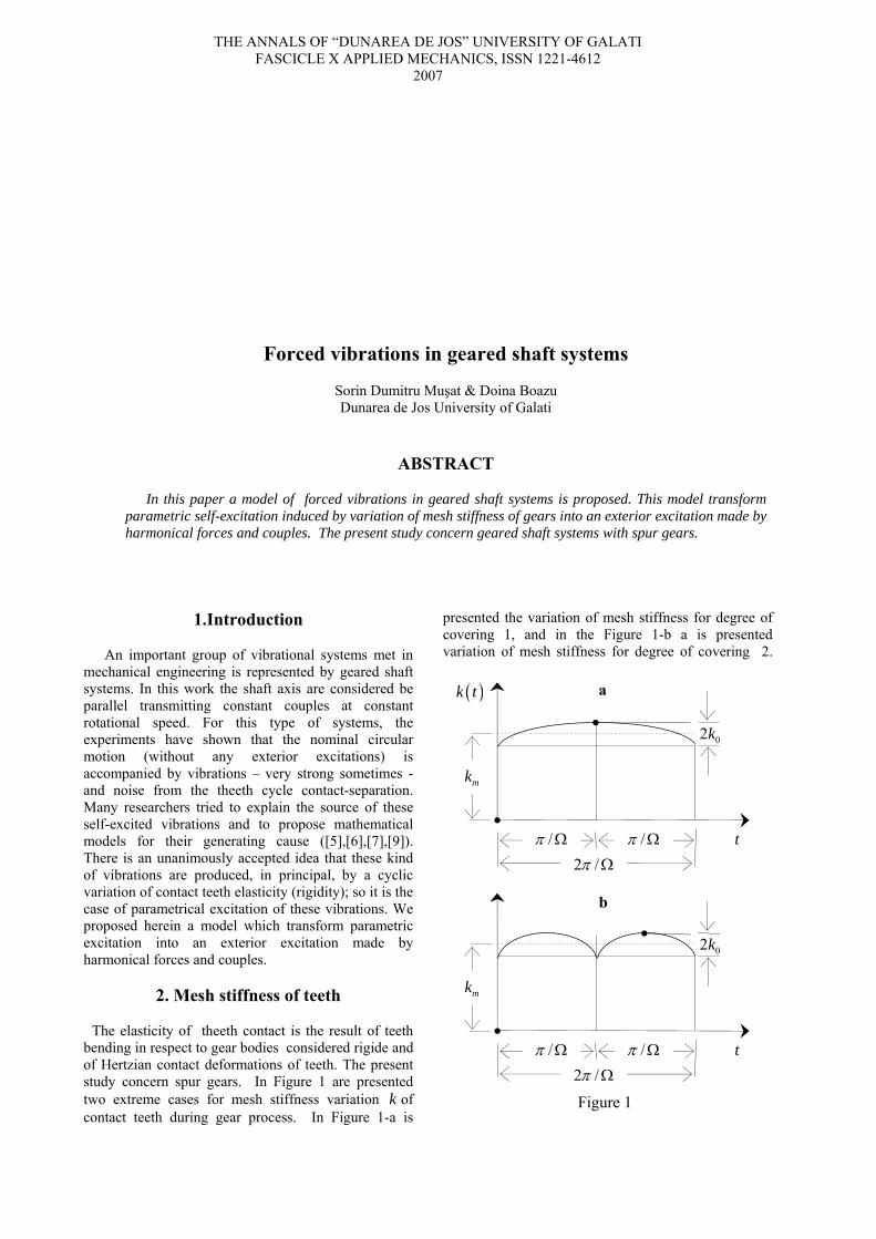
THE ANNALS OF “DUNAREA DE JOS” UNIVERSITY OF GALATI FASCICLE X APPLIED MECHANICS, ISSN 1221-4612
2007
Forced vibrations in geared shaft systems
Sorin Dumitru Muşat & Doina Boazu Dunarea de Jos University of Galati
ABSTRACT
In this paper a model of forced vibrations in geared shaft systems is proposed. This model transform parametric self-excitation induced by variation of mesh stiffness of gears into an exterior excitation made by harmonical forces and couples. The present study concern geared shaft systems with spur gears.
1.Introduction
An important group of vibrational systems met in mechanical engineering is represented by geared shaft systems. In this work the shaft axis are considered be parallel transmitting constant couples at constant rotational speed. For this type of systems, the experiments have shown that the nominal circular motion (without any exterior excitations) is accompanied by vibrations – very strong sometimes - and noise from the theeth cycle contact-separation. Many researchers tried to explain the source of these self-excited vibrations and to propose mathematical models for their generating cause ([5],[6],[7],[9]). There is an unanimously accepted idea that these kind of vibrations are produced, in principal, by a cyclic variation of contact teeth elasticity (rigidity); so it is the case of parametrical excitation of these vibrations. We proposed herein a model which transform parametric excitation into an exterior excitation made by harmonical forces and couples.
2. Mesh stiffness of teeth
The elasticity of theeth contact is the result of teeth
bending in respect to gear bodies considered rigide and of Hertzian contact deformations of teeth. The present study concern spur gears. In Figure 1 are presented two extreme cases for mesh stiffness variation of contact teeth during gear process. In Figure 1-a is
presented the variation of mesh stiffness for degree of covering 1, and in the Figure 1-b a is presented variation of mesh stiffness for degree of covering 2.
k
t
02k
( )k t
mk
2 /π Ω
/π Ω /π Ω
t
02k
mk
2 /π Ω
/π Ω /π Ω
Figure 1
a
b

FASCICLE X THE ANNALS OF “DUNAREA DE JOS” UNIVERSITY OF GALATI
We denote circular frequency of gearing by Ω . Harmonical variation of mesh stiffness and the shape of curves from Figure 1 give the reason to aproximate this variation by means a harmonical function,
( ) ( )0 cosmk t k k t= − Ω , (1)
where is the mean value, is the amplitude of fluctuations.
mk 0k
3. Parametric excitation modeling using harmonical excitation
Mechanical model for parametric vibrations
produced by cyclic variations of mesh stiffness is the one from Figure 2, where ,a bJ J are the moments of inertia of gears, radii of the base circles of gears, ,a br r
,a bM M reduced mass of gears along line of action
( 2 2/ , /a a a b b bM J r M J r= = ).
Equations of motion of the two masses are:
( )( )( )( )
0,0.
a a b a
b b b a
M x k t x xM x k t x x
− −+ −
&&
&&
==
a
For remove the body motion of the system it is introduced the relative displacement of masses,
bx x x= − , and we substract the two equations. It is obtained:
( )2 01 cos 2m
kx p t xk
⎛ ⎞+ − Ω =⎜ ⎟
⎝ ⎠&& 0,
(2) where
m m
a b
k kpM M
= +
is natural circular frequency of the system for ct.mk k= =
Equations (2) is a differential equation of Mathieu type. The possibility of some instable motions (some increased amplitude indefinit in time) results from diagrams represented in Figure 3-a (using [4]). It can
range of values of
observe that for (situation of interest) the 0 / 1mk k
Ω for instable motion is reduced at precise values / , 1,2,...p j jΩ = = (3) If between the two rom Figure 2 we masses of system fconsider a viscous damper, the shape of diagrams become those from Figure 3-b. For values of Ω given by (3) the motion of system becomes instable (vibration with finit amplitude). The size of segments A A− , B B− , C C− represents a measure of
d g effect for situ tions illustrated by (3). It results that for these situations the amplitude of vibration decreases for increased values of j . The problems presented above show that for ( in studied cases the ratio 0 / <0.1mk k ) parametrical vibrations (self-parametric) m from Figure 2 can be proper modeled considerring
ampin a
of syste
( ) constantmk t k= = and introducing on the line of tion forces or cinematic periodic
excitation with period 2 /Taction periodic excita
π= Ω . We admit a kinematic excitation as in th with e Figure 4
( ) ( )0 sinx t x t= Ω (4) which determines resonance only for pΩ =
C C
B B
A A
0
01
0 / mk k
/ pΩ
0.2 0.6 0.8 0.4
1
1/ 2
1/ 3
1 0 / mk k
/ pΩ
0.2 0.6 0.8 0.4
1
1/ 2
1/ 3
Figure 3
ar
br
bx ax
aM bM ( )k t
Line of action
Figure 2
34
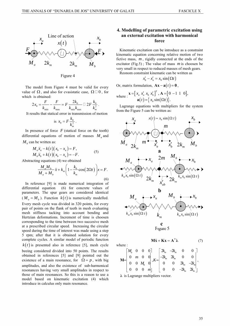
THE ANNALS OF “DUNAREA DE JOS” UNIVERSITY OF GALATI FASCICLE X
The model from Figure r every va
ob
4 must be valid folue of Ω , and also for cvasistatic case, 0Ω , for
which is tained: 0 0
0 2min max min max
22 Fx = − 2m
k kF F Fk k k k k
= .
It results that statical error in transmission of motion
is 0kx F= . 0 2mk
In presence of force F (statical force on the tooth) differential equations of motion of masses aM and
bM can be written as:
( )( )( )( )
,.
a a b a
b b b a
M x k t x x FM x k t x x F
− =+ − = −&&
(5)
Abstracting equations (4) we obtained
−&&
( )0a bM M k1 cos 2 .ma b m
x k t xM M k
⎞+ − Ω =⎜ ⎟+ ⎝ ⎠
&&
(6) In reference [9] is made numerical integration
di
F⎛
of fferential equation (6) for concrete values of
parameters. The spur gears are considered identical ( a bM M= ). Function ( )k t is numerically modelled. E cycle was d d in 320 points, for every pair of points on the flank of teeth in mesh evaluating mesh stiffness tacking into account bending and Hertzian deformations. Increment of time is choosen corresponding to the time between two succesive mesh at a prescribed circular speed. Increasing the circular speed during the time of interest was made using a step 5 rpm; after that it is obtained solution for every complete cycles. A similar model of periodic function (
very mesh ivide
)k t is presented also in reference [5], mesh cycle g considered divided into 50 points. The results
obtained in references [5] and [9] pointed out the existence of a main resonance, for
beein
pΩ = , with big amplitudes, and also the existence of su armonical resonances having very small amplitudes in respect to those of main resonances. So this is a reason to use a model based on kinematic excitation (4) which introduce in calculus only main resonance.
4. Modelling of parametric excitation using an external excitation with harmonical
force
b-h
Kinematic excitation can be introduce as a constraint
kinematic equation concerning relative motion of two fictive mass, , rigidly connected at the ends of the excitator (Fig.5) ; The value of mass m is choosen be very small in respect to reduced masses of mesh gears.
m
Reonom constraint kinematic can be written as ( )0 sinb ax x x t′ ′− = Ω
Or, matrix formulation, ( )t− =Ax a 0 ,
where : [ ] [( ) ( )
T
0
, 0 1 1 0sin .
a a b bx x x xt x t′ ′= = −= Ω
x Aa
],
Lagrange equations with multipliers for the system from the Figure 5 can be written as:
T+ =Mx Kx A λ&& (7) where :
2 2 0 00 0 02 2 0 00 0 0
, ,0 0 2 20 0 00 0 2 20 0 0
m ma
m m
m mb
m m
k kMk km
Kk kMk km
−⎡ ⎤⎡ ⎤⎢ ⎥⎢ ⎥ −⎢ ⎥⎢ ⎥= =⎢ ⎥⎢ ⎥ −⎢ ⎥⎢ ⎥
−⎣ ⎦ ⎣ ⎦
M
λ is Lagrange multipliers vector.
bM
2 mk ( )0 sinmk x tΩ
( )0 sinmk x tΩ
ax
a
( )0 sinmk x tΩ
bx
2 mk
ax
( ) (0 sin )x t x t= Ω
m
max′
bx ax
aM bM 2 mk 2 mk bx′
Figure 5
b
2m
( )0 sinmk x tΩ
bx
mk
c
abx′
aM
aM bM
F F( )x t
bx ax
aM bM 2 mk
Line of action
2 mk
Figure 4
35

FASCICLE X THE ANNALS OF “DUNAREA DE JOS” UNIVERSITY OF GALATI
Lagrange multipliers can be removed using the matrix , the natural orthogonal complement of matrix (2],[3]) with property:
BA
TT, .= =AB 0 B A 0 Any of displacements ax′ or bx′ can be seen as a
dependent one. By choosen the displacement bx′ as dependent one the displacement vector is partitioned in form:
x
cu , a
a
b
x
bx xx
⎧ ⎫⎧ ⎫ ⎪ ⎪′= =⎨ ⎬ ⎨ ⎬⎩ ⎭ ⎪ ⎪
⎩ ⎭
xx = x x
x%
% ′ (8)
And the matrix A in form :
[ ] [ ] with 0 1 0 , 1 .⎡ ⎤ = − =⎣ ⎦A = A A A A% %
It can be written relations : ( ) ( ) ( ), ,t t+ = + +x = Bx b x Bx b x = Bx b& &% & % % t (9)
where :
( ) ( )11 , tt−−
⎧ ⎫⎡ ⎤= = ⎨ ⎬⎢ ⎥ −−⎣ ⎦ ⎩ ⎭
0IB b
A aA A% .
By introducing transformations Introducând transformările (9) into (7) and premultiplying with
the Lagrange multipliers are removed and we obtain
TB
( )t+ =Mx Kx f&&% %% % where :
T
0 0 0 2 0 ,
0 0
a
b
Mm
M
⎡ ⎤⎢ ⎥= = ⎢ ⎥⎢ ⎥⎣ ⎦
M B MB%
T
2 2 0 2 4 2 ,
0 2 2
m m
m m m
m m
k kk k k
k k
⎡ ⎤⎢ ⎥= = ⎢ ⎥⎢ ⎥⎣ ⎦
K B KB%
( ) ( ) ( ) ( )T T0
20 0
0
sinwith
0 2 .
2a m
m
t t t
mx k xk x
= − − = Ω
⎧ ⎫⎪ ⎪= Ω −⎨ ⎬⎪ ⎪⎩ ⎭
f B Mb B Kb f
f
&& t
By considering ax′ as dependent and by following
the above procedure we can obtained the same matrices şi ; the vector becomes M% K% 0f
02
0
22
0
m
a m
k xmx k x
−⎧ ⎫⎪ ⎪= − Ω +⎨⎪ ⎪⎩ ⎭
f 0 .⎬ (10)
For obtaining a simetrical solution the cinematic excitation is decomposed into two identical components by using one of them in removing of bx′ . By overlapping effects of the two cinematic excitations
one obtains 0
0
0
0m
m
k x
k x
−⎧ ⎫⎪ ⎪= ⎨ ⎬⎪ ⎪⎩ ⎭
f (11)
that means an average of the vectors determined in the above procedure.
We hold differential equations in form
( )0
0
0 0 00 2 0 2 0 sin0 0
a a m m a m
ab m m m ab
b b m m m b m
M x k k x k xm x k k k x
M x k k k x k x
− −⎧ ⎫ ⎧ ⎫ ⎧ ⎫⎡ ⎤ ⎡ ⎤⎪ ⎪ ⎪ ⎪ ⎪ ⎪⎢ ⎥ ⎢ ⎥′ ′ t+ − − =⎨ ⎬ ⎨ ⎬ ⎨ ⎬⎢ ⎥ ⎢ ⎥⎪ ⎪ ⎪ ⎪ ⎪ ⎪⎢ ⎥ ⎢ ⎥− −⎩ ⎭ ⎩ ⎭ ⎩ ⎭⎣ ⎦ ⎣ ⎦
&&
&&
&&
Ω
(12)
Which describe the motion of the system from the Figure 5-b.
The value of mass m can be however small. At limit, considering , we obtain the system from Figure 5-c with the motion describes by the equations
0m →
( )0
0
0sin
0a a m m a m
b b m m b m
M x k k x k xt
M x k k x k x− −⎧ ⎫ ⎧ ⎫ ⎧ ⎫⎡ ⎤ ⎡ ⎤
+ = Ω⎨ ⎬ ⎨ ⎬ ⎨ ⎬⎢ ⎥ ⎢ ⎥−⎩ ⎭ ⎩ ⎭ ⎩ ⎭⎣ ⎦ ⎣ ⎦
&& &&
&& &&
(13)
Harmonical excitations from the right member of equations generally excites coupling vibrations (torsional and bending of geared shafts.
The model proposed by equations (13) can be olso obtained by method of fictious potential ([1]). The values of mesh stiffness are bigger that shafts stiffness (from modeling of geared shaft system using FEM); elastic elements of stiffness model rigid transmission of motion -Figura 6-a.
mk
mk
Equation of kinematic constraint given by the kinematic excitation is written:
( ) 0 sin 0c x t= − ΩAx = (14) where
[ ] [ ]T , 1 1a bx x= = −x A . Kinetic energy of system from Figure 6-a is
T12E= x Mx& & .
The fictious potential associated to kinematic
constraint ([1]) is
212V= cα
where α is a penalty factor with very large value. Tacking into account (14) fictious potential can be express as
36

THE ANNALS OF “DUNAREA DE JOS” UNIVERSITY OF GALATI FASCICLE X
( ) ( ) ( ) ( )( ) ( )
TT T10 02
T T T T 2 210 02
V sin sin
sin sin
x t x t
x t x t
α
α α α
= − Ω − Ω
= − Ω + Ω
x A Ax
x A Ax x A
=
Lagrange equations
E E Vddt
∂ ∂ ∂⎛ ⎞ − + =⎜ ⎟∂ ∂ ∂⎝ ⎠0
x x x&
lead to differential equations ( )( )
0
0
0 sinsin0
a a a
b b b
M x x x tM x x x t
αα ααα α− Ω⎧−⎧ ⎫ ⎧ ⎫⎡ ⎤ ⎡ ⎤
+ =⎨ ⎬ ⎨ ⎬ ⎨ ⎬⎢ ⎥ ⎢ ⎥ Ω−⎣ ⎦⎩ ⎭ ⎩ ⎭⎣ ⎦ ⎩
&&
&&
⎫
⎭ (15)
The equations (15) describe the motion of system from Figure 6-b; these will describe the motion of system from Figure 6-a if α →∞ . Value of mesh stiffness of the real system fullfil condition of imposed size for
mkα (this value
practically models rigid body motion) so admitting mkα = (Fig. 6-c) it is accomplished a theoretical
acurate modeling of system motion described by equations (15).
References
1. BAYO, E., SERNA, M.A., 1989, Penalty formulation for the dynamic analysis of elastic mechanisms, Journal of Mechanisms, Transmissions and Automation in Design, 111, pp.321-327.
2. BLAJER,W., 1992, A projection method approach to consrained dynamic analysis, ASME Journal of Applied Mechanics, 59, pp.643-649.
3. BLAJER,W., BESTLE, D. and SCHIEHLEN, W., 1994, A projection method approach to constrained
dynamic analysis, ASME Journal of Mechanical Design , 116, pp.423-428.
4. BOLOTIN, W.W., 1961, Kinetische stabilitat elastischer systeme, DVW, Berlin.
5. OZGUVEN, H.N. AND HOUSER, D.R., 1988, Dynamic analyses of high speed gears by using loaded static transmission error, Journal of Sound and Vibration, 125, pp.71-83.
6. OZGUVEN, H.N., 1991, A non-linear mathematical model for dynamic analysis of spur gears including shaft and bearing dynamics, Journal of Sound and Vibration, 145, pp.239-260.
bM
( )0 sinx tα Ω
( )0 sinmk x tΩ
ax
a
( )0 sinx tα Ω
bx ax
( ) ( )0 sinx t x t= Ω ax
bx
aM bM
Figure 6
b
( )0 sinmk x tΩ
bx
mk
c
aM
aM bM
α
37

FASCICLE X THE ANNALS OF “DUNAREA DE JOS” UNIVERSITY OF GALATI
7. ŞENER, O.S. AND OZGUVEN, H.N., 1993, Dynamic analysis of geared shaft systems by using a continuous system model, Journal of Sound and Vibration, 166, 3, pp.539-556.
8. UMEZAWA, K., AJIMA, T., HOUJOH, H., Vibration of three axes gear system, Buletin of JSME, 27, 29,249, 1996, pp.590-597.
9. UMEZAWA, K., SATO,T., ISHIKAWA, J., Simulation on rotational vibration of spur gear, Buletin of JSME, 27, 223, 1984, pp.102-109.
38

THE ANNALS OF “DUNAREA DE JOS” UNIVERSITY OF GALATI FASCICLE X APPLIED MECHANICS, ISSN 1221-4612
2007
Shape Design For Elastic Contact Problems
Doina Boazu “Dunarea de Jos” University of Galati
ABSTRACT
In this work, a method of optimized contact surface in such a way that the contact reactions
between the two surfaces are to be uniform. To achieve an optimum profile of indenter was used finite element method. The presented procedure concern problems of conform contact between elastic bodies, without considering friction.
KEY WORDS: Sensitivity analysis, Contact problems, FEM Modeling
1. Introduction
Many mechanical structures are built from two or more parts. Forces transmission between these parts is achieved by mechanical contact. Excessively high contact forces have an important influence on performance, reliability and lifetime of the structures involved. The goal of this study is modifying the profile of indentor in such a way that the contact reactions between the two elastic bodies are to be uniform. 2. The principle of method
Between the two elastic discretized bodies,
along the contact edge (for 2D problems) were generated truss elements normal to contact surfaces. Shape modification of contact zone to achieve an optimum profile of indenter is created by the difference between reactions from external load and the uniform imposed reactions along the contact edge. The optimized profile of indenter arise from a superposition of two effects: one is the effect of external load and the second one is the imposed effect of uniform reactions in the contact zone. The proposed “optimization” is not an iterative process as in the references [1] and [2].
For conform contact problems (the problem which the extension of contact zone is known a priori), one can obtain an optimized profile of contact zone using the following relation:
_ _contact optimized contact exterior uniform imposedK u F F⎡ ⎤ ⋅ + =⎣ ⎦
where Kcontact is the rigidity matrix of contact domain, uoptimized is the displacement vector corresponding to optimiyed profile of indentor, Fcontact_exterior is reactions vector of contact zone because of exterior load , vector Funiform_imposed contain uniform reactions in contact domain.
The obtained “optimized” profile is dependent of mesh density in the contact zone. Using a mesh one can obtain a “zig-zag” profile and non-uniformities at the external edges.
3. Numerical examples
The proposed technique is applied to solve the two-dimensional shape optimization problems of elastic contact. The illustrative examples presented herein include typical contact cases of elastic vs elastic bodies. A more practical contact problem of a seal surface design is also investigated. In the study,

FASCICLE X THE ANNALS OF “DUNAREA DE JOS” UNIVERSITY OF GALATI
the design objective is to seek a uniform contact stress distribution over the entire contact surfaces.
Example 1: Contact between two elastic bodies
In this example, two elastic bodies B1 and B2 come into contact under a uniformly distributed far field compressive load of P = 1.0 MPa. The
Young’s modulus of the elastic material is 15.0MPa for B1 and 1.0 MPa for B2, Poisson’s ratio is 0.3 for both. The plane stress finite element model of the contact system is illustrated in Figure 1. In the evolutionary iteration, the contact boundary on B1 is considered as the design domain and the re-meshing process will be carried out over the entire region of body B1.
Fig. 1 Two elastic bodies in contact
Fig. 2 FEA model of contact with elastic body
Figure 4 shows the initial and optimal contact stress distributions on the contact surface. In the initial design, a distinct edge singularity (ie. a very sharp
increase in contact stress near the corner) can be observed. The final design has a constant distribution of contact stress. Figure 3 displays a sketch of the
40

THE ANNALS OF “DUNAREA DE JOS” UNIVERSITY OF GALATI FASCICLE X
optimized contact profile. It is found that the profile is similar to the traditional punch design. The
rigidity matrix of contact domain Kcontact , named kk have the following elements
kk(1,1)=2563.47; kk(1,2)=-1949.73; kk(1,3)=-780.75; kk(1,4)=-211.27; kk(1,5)=-131.621; kk(1,6)=-52.9104; kk(1,7)=5.10714; kk(1,8)=64.0076; kk(1,9)=131.109; kk(1,10)=217.446; kk(1,11)=145.15; kk(2,2)=5989.78; kk(2,3)=-2805.47; kk(2,4)=-1259.17; kk(2,5)=-412.296; kk(2,6)=-231.446; kk(2,7)=-76.2815; kk(2,8)=44.1198; kk(2,9)=168.001; kk(2,10)=315.052; kk(2,11)=217.446; kk(3,3)=7462.22; kk(3,4)=-2486.62; kk(3,5)=-1131.99; kk(3,6)=-347.735; kk(3,7)=-197.221; kk(3,8)=-60.0812; kk(3,9)=48.5399; kk(3,10)=168.001; kk(3,11)=131.109; kk(4,4)=7770.46; kk(4,5)=-2333.67; kk(4,6)=-1045.39; kk(4,7)=-302.866;
kk(4,8)=-179.552; kk(4,9)=-60.0811; kk(4,10)=44.1199; kk(4,11)=64.0076; kk(5,5)=7874.26; kk(5,6)=-2274.1; kk(5,7)=-1019.33; kk(5,8)=-302.866; kk(5,9)=-197.221; kk(5,10)=-76.2813; kk(5,11)=5.10719; kk(6,6)=7903.16; kk(6,7)=-2274.1; kk(6,8)=-1045.39; kk(6,9)=-347.734; kk(6,10)=-231.446; kk(6,11)=-52.9103; kk(7,7)=7874.26; kk(7,8)=-2333.66; kk(7,9)=-1131.99; kk(7,10)=-412.295; kk(7,11)=-131.621; kk(8,8)=7770.46; kk(8,9)=-2486.62; kk(8,10)=-1259.62; kk(8,11)=-211.27; kk(9,9)=7462.22; kk(9,10)=-2805.47; kk(9,11)=-780.75; kk(10,10)=5989.78; kk(10,11)=-1949.73; kk(11,11)=2563.47;
Fig. 3 Optimized profile of indenter
Fig. 4 Stress distribution on the contact surface Example 2: Design of axisymmetric seal surface
In engineering design, the sealed surface between two components is often required to have a
uniform contact stress for the reliability and duration of seal functionality. In this example, a sealing surface of two elastic bodies B1 and B2 with axisymmetric shapes is to be designed. A 10 kN point
41
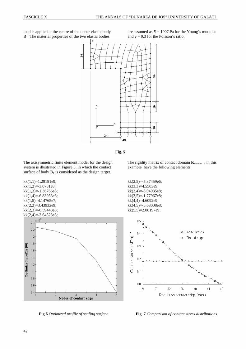
FASCICLE X THE ANNALS OF “DUNAREA DE JOS” UNIVERSITY OF GALATI
load is applied at the centre of the upper elastic body B1. The material properties of the two elastic bodies
are assumed as E = 100GPa for the Young’s modulus and v = 0.3 for the Poisson’s ratio.
Fig. 5
The axisymmetric finite element model for the design system is illustrated in Figure 5, in which the contact surface of body B1 is considered as the design target.
The rigidity matrix of contact domain Kcontact , in this example have the following elements:
kk(1,1)=1.29181e9; kk(1,2)=-3.0781e8; kk(1,3)=-1.36766e8; kk(1,4)=-6.83953e6; kk(1,5)=4.14765e7; kk(2,2)=3.43932e9; kk(2,3)=-6.59443e8; kk(2,4)=-2.64523e8;
kk(2,5)=-5.37459e6; kk(3,3)=4.5503e9; kk(3,4)=-8.04035e8; kk(3,5)=-1.77967e8; kk(4,4)=4.6092e9; kk(4,5)=-5.63008e8; kk(5,5)=2.08197e9;
Fig.6 Optimized profile of sealing surface
Fig. 7 Comparison of contact stress distributions
42

THE ANNALS OF “DUNAREA DE JOS” UNIVERSITY OF GALATI FASCICLE X
Shown in Figure 7 is the comparison of the contact stress distributions in the initial and the final designs. A uniform stress distribution in the entire sealing ring area has been obtained through the
evolutionary modification on the sealing surface. Figure 6 shows the optimized profile of sealing surface. This is expected to enhance the sealing effect and duration, especially if cyclic loading is involved.
4. Concluding remarks
This study has demonstrated that the proposed technique can solve shape optimization for elastic contact problems with and without friction. Compared with the existing mathematical programming based methods, the greatest advantage of this technique is its simplicity and stability. This
procedure can be easily integrated into the standard finite element codes by just adding a few lines to gradually adjust the gap spacing between two contact bodies.
The proposed approach can be extended to more contact problems such as bending plates and three- dimensional bodies and possibly to large deformation process such as metal forming.
References
[1] Okamoto, N. and Nakazawa, M., "Finite Element Incremental Contact Analysis with Various Frictional Conditions", Int. J. Numer. Meth. Engng, Vol. 14, pp. 337-357, 1979.
[2] Tseng, J. and Olson, M.D., "The Mixed Finite Element Method Applied to Two-dimensional Elastic Contact Problems", Int. J. Numer. Meth. Engng., Vol. 17, pp. 991-1014, 1981.
[3] Sachdeva, T.D. and Ramakrishnan, C.V., "A Finite Element Solution for the Two-dimensional Elastic Contact Problems with Friction", Int. J. Numer. Meth. Engng., Vol. 17, pp. 1257-1271, 1981.
[4] Zhong, Z.H., Finite Element Procedures for Contact-impact Problems, Oxford University Press Inc., New York, 1993.
[5] Aliabadi, M.H. and Brebbia, C.A., Computational Methods in Contact Mechanics, Computational Mechanics Publications Southampton Boston, 1993.
[6] Conry, T.F. and Seireg, A., "A Mathematical Programming Method for Design of Elastic Bodies in Contact", ASME Transactions J. Appl. Mech., pp.387 -392, June 1971.
[7] Haug, E.J. and Kwak, B.M., "Contact Stress Minimization by Contour Design", Int. J. Numer. Meth. Engng., Vol.12, pp. 917-930, 1978.
[8] Cheng, W.Q., Zhu, F.W. and Luo, J.W., "Computational Finite Element Analysis and Optimal Design for Multibody Contact System", Comp. Meth. Appl. Mech. & Engng., Vol. 71, pp.31-39, 1988.
[9] Belegundu, A.D. and Chandrupatla, T.R., "Shape Optimization of Valve Geometry with Contact Analysis",
Sensitivity Analysis and Optimization with Numerical Methods, AMSE (edited by Saigal, S. and Mukherjee, S.), pp.71-78, 1990.
[10] Park, J. and Anderson, W.J., "Geometric Optimization in Presence of Contact Singularities", AIAA Journal, Vol. 33, No. 8, pp. 1503-1509, 1995.
[11] Fancello, E.A. and Feijoo, R.A., "Shape Optimization in Frictionless Contact Problems", Int. J. Numer. Meth. Engng., Vol.37, pp. 2311-2335, 1994.
[12] Fancello, E.A., Haslinger, J. and Feijoo, R.A., "Numerical Comparison Between Two Cost Functions in Contact Shape Optimization", Structural Optimization, Vol. 9, No. 1, pp.57-68, 1995.
[13] Tada, Y. and Nishihara, N., "Optimum Shape Design of Contact Surface with Finite Element Methods", Advances in Engineering Software, Vol. 18, pp.75-85, 1993.
[14] Xie, Y.M. and Steven, G.P., "A Simple Evolutionary Procedure for Structural Optimization", Comp. & Struct., Vol. 49, pp. 885-896, 1993.
[15] Xie, Y.M. and Steven, G.P., Evolutionary Structural Optimization, Springer-Verlag, Berlin, 1997.
[16] Galin, L.A., "Contact Problems in the Theory of Elasticity" (edited by Sneddon, I.N.), North Carolina State College Translation, 1961.
[17] Oden, J.T. and Carey, G.F., Finite Elements : Special Problems in Solid Mechanics, Volume V, Prentice-Hall Inc., New Jersey, 1984.
[18] Zhong, Z.H and Mackerle, J., "Static Contact Problems - A Review", Engineering Computations, Vol. 9, pp. 3-37, 1992.
43

FASCICLE X THE ANNALS OF “DUNAREA DE JOS” UNIVERSITY OF GALATI
[19] Zhong, Z.H and Mackerle, J., "Contact-impact Problems: A Review with Bibliography", ASME Transactions, Appl. Mech. Rev., Vol. 47(2), pp. 55-76, 1993.
[20] Seireg, , A.A. and Rodriguez, J., Optimizing the Shape of Mechanical Elements and Structures, Marcel Dekker, Inc., New York, 1997.
44

THE ANNALS OF “DUNAREA DE JOS” UNIVERSITY OF GALATI FASCICLE X APPLIED MECHANICS, ISSN 1221-4612
2007
A MATLAB Toolbox Associated with Spectral Wave Modelling
Eugen Rusu Dunarea de Jos University of Galati
ABSTRACT A MATLAB toolbox with capabilities for visualizations data pre and post processing has been designed and associated with the state of the art spectral numerical wave models. At its first level, this computational environment facilitates the visualization and transformation of the main input fields (bathymetry, wind, current and tide), usu-ally required by the wave models. At the second level, after running the wave model, the interface allows the visualization of the model output both in space and time frames. Some additional wave parameters in relationship with the standard model output are also computed in the post processing phase. The proposed system was designed first for SWAN, bringing the advantage of a quick model implementation in a specific site com-bined with a comprehensive visualization of the simulation results. The MATLAB inter-face was further extended by adapting it for the generation models WAM and WW3, and in present can be easily associated with any other existent wave model. Moreover, con-nections with ocean and coastal circulation models, like POM or SHORECIRC, have been also accomplished. A special module for analysis in the time domain that allows both direct comparisons with in situ or remotely sensed measurements and statistical analyses was also developed. Moreover, a direct link with other MATLAB toolboxes available in the public domain and with the R environment for statistical computing and graphics, was also accomplished enlarging in this way considerably the area of appli-cability of this tool.
1. Introduction Third generation phase averaging models are
nowadays used on a wider scale. They can be genera-tion models as WAM (WAMDI Group. 1988) and WW3 (Tolman, 1999), or transformation models as SWAN (Booj et al., 1999) and STWAVE (Smith et al., 2001).
The physics for the transformation scale is more elaborated to account better for the processes specific in the coastal environment as refraction, shoaling, breaking or triad wave-wave interactions. As regards SWAN has to be underlined that in the last versions it goes beyond the condition of a model only for trans-
formation scales its range being extended in both di-rection, offshore and nearshore.
Most of the model codes are available free on the Internet. However the implementation of a wave model usually requires some specific tools for gener-ating and visualizing the input. Model outputs should be also visualized even from the first phase to verify that the model is running correctly and to identify any possible problem.
Various complex professional engineering soft-ware packages including wave modeling together with flow simulations are commercially available. They are usually designed in integrated modular frameworks with add-on modules including software for data processing visualization and post processing.
FASCICLE X THE ANNALS OF “DUNAREA DE JOS” UNIVERSITY OF GALATI ___________________________________________________________________________
In the USA, the most popular commercially avail-able software package associated with wave and near-shore current modelling is: Surface Water Modelling System (SMS) developed by Environmental Model-ling Systems, Inc. SMS includes the coastal wave models STWAVE and CGWAVE.
In Europe, two commercial packages are consid-ered in the top. These are DELFT3D, developed by Delft Hydraulics, and MIKE (version 21 for free sur-face flow and version 3 which is a fully 3D modeling package), developed by the Danish Hydraulic Insti-tute. Delft3D contains the second-generation model HISWA and its successor SWAN, while MIKE in-cludes five wave models (two spectral and other three based on the momentum concept).
All these packages support coastal circulation modeling, for either 3D or 2D flows, with advanced finite-element or finite-difference models. However the utilization of these packages is still not an easy task and requires a high degree of training and quali-fications.
The present work describes an alternative to the existent software which has the advantage of the sim-plicity and flexibility. This is a MATLAB interface with capabilities for data pre processing visualizations and post processing that was associated initially with SWAN and further extended to be used in relation-ship with most of the current operating wave and cir-culation models.
2. Options for pre processing of the input fields
The interface developed herewith is composed by
two modules which are independent but can interact at various levels. These are the pre processor and the module for analysis and post processing of the model output. In the pre processing phase are available all the standard capabilities for reading, visualizing and preparing of the input data fields according to the requirements of the various wave models.
The most usual input fields in wave modelling are bathymetry, tide, wind and currents. The sequence for pre processing is illustrated in Figure 2 for a case study domain in Campese Bay, Giglio Island in the Mediterranean Sea. Three different data sets are avail-able in the considered area, deep water bathymetry, shallow water bathymetry and coast line.
The scattered bathymetric data given in digital format x-y-z in spherical coordinates (longitude-latitude-depth) are first transformed in Cartesian co-ordinates using a Universal Transverse Mercator (UTM) projection via M_MAP software package (Pawlowicz, 2004) that is connected to the pre proc-essor. UTM are ellipsoidal projections and they are usually considered more appropriate for regions less than a few degrees in longitude. Nevertheless, most of the other standard projections are also available and
can be used after case. In this particular case, the Car-tesian coordinates are preferred because the connec-tion with some nearshore circulation models becomes simpler. The same sequence can be further followed without changing the coordinate system from spheri-cal to Cartesians.
The next step is to define the grid by giving its characteristics, the coordinates of the origin, grid rota-tion, number of meshes and lengths in x and y direc-tions, respectively, or alternatively in longitude and latitude. The grids can be defined either graphically or numerically. In the first case the origin and the oppo-site corner point are graphically selected directly on the map while the grid spacing and the angle of the grid rotation may be introduced as numerical inputs. The option to generate a rotated grid is important be-cause in areas where the nearshore currents are going to be evaluated one of the grid axes should approxi-mate the shore-normal direction. A cubic interpola-tion method based on Delaunay triangulation is ap-plied for grid generation. In areas where bathymetric data are missing, the nearest neighbour method is coupled with cubic interpolation to fill the gaps. A bathymetric map, where the land is coloured in brown and the water in various nuances of blue according to the depth darker as the depth increases, is associated to each grid.
As showed in Figure 1 each step can be visualized giving in this way the possibility to perform various corrections. Of course, some steps for processing the bathymetric data as the grid generation, reshaping or rotation, are specific only for the regular grids. How-ever the visualizations of the scattered data or of the grids and the design of the isomaps are valid also for the case of the curvilinear grids.
3. Data transfer from model to the compu-tational environment
Initially the SWAN model was used as a refer-
ence, and because of this all the SWAN output pa-rameters have correspondents into the interface. Moreover, for the SWAN model a particular module for setting the model simulations in the form of a user friendly window was developed as well.
The following sequence must be repeated for each model simulation. The bottom grid automatically de-fines the computational grid used for the SWAN simulations and the characteristics, as contained in the bathymetric driver generated together with the bathy-metric grid, are written to the SWAN input file. The number of wave directions is fixed at 36 with the op-tion that the spectral directions cover the full circle.
Thus a 10-degree resolution is achieved in direc-tional space. The number of frequencies considered is 35 with the frequency range between 0.04 and 1 Hz. Of course these parameters can be also tuned.

THE ANNALS OF “DUNAREA DE JOS” UNIVERSITY OF GALATI FASCICLE X ___________________________________________________________________________
Figure 1: Bathymetric data transformation, from scatter data to the bathymetric map (Campese bay, Giglio Island in the Mediterranean Sea south of Tuscany).
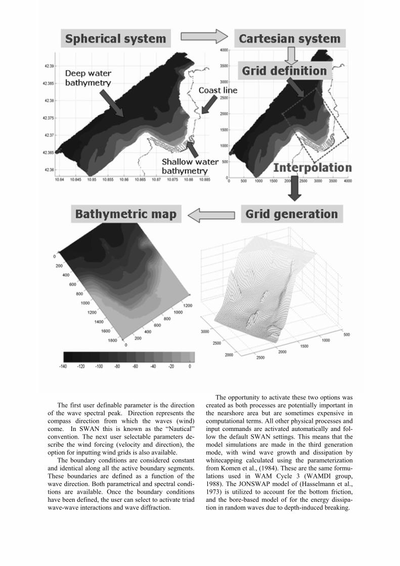
FASCICLE X THE ANNALS OF “DUNAREA DE JOS” UNIVERSITY OF GALATI ___________________________________________________________________________
The first user definable parameter is the direction
of the wave spectral peak. Direction represents the compass direction from which the waves (wind) come. In SWAN this is known as the “Nautical” convention. The next user selectable parameters de-scribe the wind forcing (velocity and direction), the option for inputting wind grids is also available.
The boundary conditions are considered constant and identical along all the active boundary segments. These boundaries are defined as a function of the wave direction. Both parametrical and spectral condi-tions are available. Once the boundary conditions have been defined, the user can select to activate triad wave-wave interactions and wave diffraction.
The opportunity to activate these two options was created as both processes are potentially important in the nearshore area but are sometimes expensive in computational terms. All other physical processes and input commands are activated automatically and fol-low the default SWAN settings. This means that the model simulations are made in the third generation mode, with wind wave growth and dissipation by whitecapping calculated using the parameterization from Komen et al., (1984). These are the same formu-lations used in WAM Cycle 3 (WAMDI group, 1988). The JONSWAP model of (Hasselmann et al., 1973) is utilized to account for the bottom friction, and the bore-based model of for the energy dissipa-tion in random waves due to depth-induced breaking.

THE ANNALS OF “DUNAREA DE JOS” UNIVERSITY OF GALATI FASCICLE X ___________________________________________________________________________
Following user input, the SWAN command file can be visualized and modified before running the model. This procedure maintains maximum flexibility in the designed system for the expert user. A general setting of the model can be made rapidly via the inter-face while for more complex situations further modi-fications can be made directly in the command file. After finishing the settings the SWAN model can be executed through the interface inside MATLAB or run in a DOS window.
The generality of this computational environment resides in the fact that it works with a unique set of variables. This includes the SWAN output and some other parameters that can be derived from them. Thus, for each model associated to the present computa-tional environment an individual program for loading the output is developed. Since in general the SWAN output includes more parameters than most of the other models if an output parameter does not exist in a specific model, automatically is associated to it in the interface the MATLAB quantity NaN (not a num-ber). Thus, in order to connect a new wave or cir-culation model to the interface it is necessary only to develop the specific MATLAB executable for loading the data.
4. Spatial analysis and post processing
Hence the only part where the post processing module interacts with the model is when it reads the output data from the wave model and loads them by allocating values to its own variables. It is thus quite simple to connect the interface to some other wave or circulation models. As regards the transfer of infor-mation was chosen the solution of making it sequen-tial that is to load the data separately for each time step. The phase and group velocities are two additional parameters computed. The phase velocities were esti-mated using the standard definitions (CERC 1984). Thus in the case of shallow water waves (when d < L/20, where d is the depth and L the wavelength) the waves are considered non dispersive and consequently the phase velocity and the group velocity are equals:
gc c gd ,= = (1)
In deep water (d > L/2):
gc 2c gL / 2 ,π= = (2)
while for the intermediate water (L/2 ≤ d ≤ L/20), results:
g
c gL / 2 tanh( 2 d / L )
1 4 d / Lc c 12 sinh( 4 d / L )
π π
ππ
=
⎛ ⎞= ⋅ +⎜ ⎟
⎝ ⎠.
(3)
A model for a quick estimation of the wind and wave contributions to the propagation of the oil on the ocean surface was implemented and connected to the wave models.
When are present tide, wind-driven currents and waves the center of the mass of the oil is supposed to move according to the equation:
dcurrent wind Stokes
dx U 0.035 U Udt
= + ⋅ +r r r r
(4)
xr is the vector defining the centre of mass of the oil
and currentUr
is the drift due to tidal currents. This tidal currents can be analysed using standard tidal analyse techniques.
The term 0.035Uwind accounts the wind-driven currents. The direction of oil spill motion induced by the wind is at a non-zero angle to the direction of the wind as a result of the Ekman effect.

FASCICLE X THE ANNALS OF “DUNAREA DE JOS” UNIVERSITY OF GALATI___________________________________________________________________________

THE ANNALS OF “DUNAREA DE JOS” UNIVERSITY OF GALATI FASCICLE X ___________________________________________________________________________
The formula proposed by Samuels et al (1982) is considered to compute the deflection angle. Accord-ing to this the wind-driven current is deflected with an angle θ to the right (clockwise) from the wind direc-tion (for the Northern Hemisphere).
38 windU25 exp 10 gθ υ−⎛ ⎞= ° −⎜ ⎟
⎝ ⎠ (4)
Where Uwind is the wind speed, g is the gravitational acceleration and υ the kinematical viscosity of the seawater. The effects of wind induced surface were modelled by the inclusion of a logarithmic velocity profile. In analogy with flow structure within a bot-tom boundary layer it was assumed that the surface layer of thickness zo moves at a velocity (typically 3.5% of the wind speed) which decays with the depth, Elliott (1986), according to:
( )( )
ow wind
c o
log z zU ( z ) 0.035 U 1
log z z⎛
= ⋅ −⎜⎜⎝
⎞⎟⎟⎠
(5)
Where zc is the depth at which the velocity is zero. It has been assumed that zc scales on the wavelength of the surface waves, i.e. zc=αL. For typical values the wind share is approximately ten times as large as that due to tidal currents. The Stokes drift was estimated using the mass transport relationship from the second order theory (Lakshmi and Clayson 2000):
( )[( )
]./2sinh
/4cosh2
)( 2
2
LdLdzC
LHzu
πππ +
⋅⋅⎟⎠⎞
⎜⎝⎛= (7)
For the deep water waves the expression (7) becomes:
( )2
sH 4u z C exp .L
π⎛ ⎞ ⎛= ⋅ ⋅⎜ ⎟ ⎜⎝ ⎠ ⎝
zLπ ⎞
⎟⎠
(8)
Finally the next option is the local data assessment, when can be selected any point from the domain and evaluate the corresponding wave parameters. The location can be defined either with graphical or nu-merical input. In order to compute the wave variables in any arbitrary point are requested from the wave model the grid data and are made bilinear interpola-tions between the grid points, in the same manner as the SWAN model does. In this way there is practi-cally no difference between the results computed by SWAN in the respective points and those provided by the interface. There is a main advantage introduced by this methodology, that is the particular locations where are needed to be seen the model results should not be declared ‘a priori’ as output locations. They can be defined only in the post processing phase and as a consequence it is increased the computational efficiency of the model simulation because of the re-
In order to simplify as much as possible the post simulation phase, the output data was structured in three distinct parts: vector fields, scalar field, and local data. The following vector fields can be repre-sented: the wave vectors (having the significant wave height as module and the mean wave direction), the swell vectors (with the significant height of the swell as module and the peak direction), the wind and cur-rent vectors, the energy transport, the wave forces and the orbital velocity. These are all direct SWAN out-put, or in the case of the wind and current are also input. The four additional quantities that were defined in the previous section, group velocity, phase veloc-
ity, wind induced current velocity and Stokes drift, may be also represented. For each vector field it was assigned a different colour, however if from visual reasons it is necessary to change this colour this can be made with the command set colour. Other set com-mands available concern the density and the scaling factor of the vector field.
The scalar fields can be represented in three ways, as: 3D plots, 2D plots or contour plots. The following parameters can be displayed: depth, significant wave height, significant height of swell (resulted by inte-grating the spectrum in the low frequency part), all the wave periods defined in SWAN (TM01, TM02, TMM10, peak period, relative mean period RTM01, average wave period and relative average wave pe-riod), wavelength, steepness, directional spreading, frequency spreading, wave power, dissipation and also wind, current and orbital velocities in absolute values. Two new parameters, the peakedness of the wave spectrum and the Benjamin-Feir index for quan-tifying the probability of freak waves, which were made available in the most recent SWAN release (40.51AB), were also introduced as scalar variables. The 2D projections and the contour plots provide similar representations of the field and the user can decide after case which of them is more appropriate. Moreover various combinations between the vector and scalar fields can be also made. For both vector and scalar fields, the maximum value of the quantity represented as well as its field location, are also given.
Figure 2a illustrates an example of the wave model output visualization in the coastal environment close to Lisbon (conditions from 2004/04/14_h12). In background is presented the significant wave height scalar field while in foreground the wave vectors. Figure 2b presents a 3D representation of the bathym-etry in the same area. In order to give a better per-spective the coast line was represented in both fig-ures.

FASCICLE X THE ANNALS OF “DUNAREA DE JOS” UNIVERSITY OF GALATI ___________________________________________________________________________ duced number of output requests. In Figure 2a to-gether with the representation of the scalar and vector fields is presented also such a local data assessment. Were evaluated in the respective point the significant wave height, the wave period (TM01) and the water depth and were compared with the maximum values existent in the entire field. Moreover the most impor-tant vectors, namely wave, wind and current, are also computed and figured.
Another interpolation scheme was designed for the local data assessment which is valid both for regular and curvilinear grids (however in the case of the regu-lar grids it is still preferred the initial interpolation scheme which seems to be faster).
An additional post processing option concerns the visualizations of the biased fields for two scalar quan-tities. This allows comparisons between different model outputs as for example significant wave height and significant swell height but also for the same pa-rameter evaluated in different conditions. Such an example is illustrated in Figure 3 for a case study re-lated to the coastal environment of the Porto Santo Island and corresponding to the time frame 2001/01/26-h09. Thus Figure 3a presents the signifi-cant wave height scalar fields and the wave vectors for the spatiotemporal frame considered. Figures 3b and 3c illustrate the Hs biased fields, positive and negative biases, respectively due to the process of diffraction. The computation of the Hs bias is per-formed in all the grid points with the following rela-tionship:
( ) ( ) ( ,,,, jiHjiHjiDH sss −+ −= ) (9) where DHs is the Hs bias, (i,j) defines the grid point, Hs+ is the significant wave height computed with the diffraction process activated while Hs- the significant wave height without activating diffraction into the model. A similar relationship is applied for any other different process considered. For this particular case, as shown in Figure 7b, diffraction has a considerable spatial impact in the computational domain consid-ered. At the edges of the island Hs enhancements of more than half a meter, representing relative incre-ments of about 40%, are induces. Another observa-tion resulting from the analysis of the above figures would be that the numerical scheme implemented to model diffraction in a phase decoupled approach in-duces also some noise in the computational domain because there is no reason to believe that diffraction might have any relevance in the north of the island. A similar case is presented in Figures 3d and 3c for the case of the triad nonlinear interactions. These triads are relevant in shallow water especially for steep waves and due to them the energy is moved to the high frequency domain. Thus Figure 3d shows that for the considered case triads modify significantly the wave field especially in the south of the island; how-ever the maximum increments in terms of significant wave height, up to one meter, are encountered in the
north of the island. On the other hand Figure 3e shows that also in the north of the island the triad nonlinear interactions can bring also decreases of the significant wave heights of almost half a meter.
5. Concluding remarks A MATLAB toolbox with capacities for data
processing and visualisations, that might be associ-ated with most of the currently operating spectral wave models, has been designed. This allows a quick implementation of the wave models in a spe-cific site and, on the other hand, a better evaluation of the model output. A special module for analysis in the time domain that allows both direct compari-sons with in situ or remotely sensed measurements and statistical analyses was also developed being connected in addition with the R computational environment for statistical computing and graphics, http://www.r-project.org/. Moreover the link with some other MATLAB toolboxes as DIWASP (Johnson 2002) and M_MAP (Pawlowicz, 2004) has been also made.
6. References
BOOIJ, N., RIS, R. C and HOLTHUIJSEN, L. H., 1999. A third generation wave model for coastal regions. Part 1: Model de-scription and validation, J. Geophys. Res. 104, C4, pp. 7649-7666.
CERC 1984. Shore Protection Manual, Coastal Engineer Research Center, U.S. Army Corps of Engrs. Washington D.C.: U.S. Govt. Printing Office.
ELLIOTT, A.J. 1986. Share Diffusion and Spread of Oil in the Surface Layers of the North Sea, Dt. Hydrogr. Z 39, 113-137.
JOHNSON, D., 2002, DIWASP, a directional wave spectra tool-box for MATLAB, User Manual, WP 1601 DJ (V1.1), i-18. Centre for Water Research, University of Western Australia.
KOMEN, G.J., S. HASSELMANN, and K. HASSELMANN, 1984: On the existence of a fully developed windsea spectrum, J. Phys. Oceanogr., 14, 1271-1285.
KUIK, A.J., G.PH. VAN VLEDDER and L.H. HOLTHUIJSEN, 1988: A method for the routine analysis of pitch-and-roll buoy wave data, J. Phys. Oceanogr., 18, 1020-1034.
LAKSHMI H. K. and CLAYSON, C. A. 2000. Small Scale Proc-esses in Geophysical Fluid Flows, AP – International Geophys-ics Series, volume 67, Academic Press, San Diego, Calif., 888 p.
PAWLOWICZ R, 2004: M_Map - A mapping package for MAT-LAB, User Manual, V 1.4, Department of Earth and Ocean Sciences, University of British Columbia, Canada.
SAMUELS, W.B., HUANG, N.E. and AMSTUTZ D.E. 1982. An Oil Spill Trajectory Analysis Model with a Variable Wind De-flection Angle, Ocean Engng. Vol. 9, Pergamon Press Ltd., 347-360.
SMITH, J. M., SHERLOCK, A. R., & RESIO, D. T. 2001 STWAVE: Steady-State Spectral Wave Model, user’s guide for

THE ANNALS OF “DUNAREA DE JOS” UNIVERSITY OF GALATI FASCICLE X ___________________________________________________________________________
STWAVE Version 3.0, ERDC/CHL SR-01-01, U.S. Army Engi-neer Research and Development Center, Vicksburg, MS.
THE MATH WORKS INC., 2004: MATLAB the Language of Technical Computing, Reference Guide, v.7.0 (Release 14).
TOLMAN, H. L., 1999 User manual and system documentation of WAVEWATCH III, Tech. Note 166, NOAA/NWS/NCEP/OMB, 99 pp.
WAMDI GROUP, 1988: The WAM model - a third generation ocean wave prediction model, J. Phys.Oceanogr., 18, 1775-1810.

THE ANNALS OF “DUNAREA DE JOS” UNIVERSITY OF GALATI FASCICLE X APPLIED MECHANICS, ISSN 1221-4612
2007
Chatter Detection Using the Main Cutting Force (1-st Part)
George C. Balan, Alexandru Epureanu
Dunarea de Jos University of Galati
ABSTRACT Li et al (1997) uses the coherence function between two crossed accelerations (in the directions: axial X and vertical Z, measured by two accelerators mounted on the tool shank), to identify chat-ter in turning. In a frame of an experiment focused on the monitoring of a lathe we registered the accelerations of the cutter-holder, for different cutting wear classes (c1 ÷ c6), where c6 means “Chatter”. 12 monitoring indices were calculated, among: X5 → Fz variation range; X6 → number of inter-sections of oscillogram Fz with its average value zF . In the second part of this paper we will demonstrate the accurate use of these indices values for chatter detection. In this first part of the paper we present the state of the art and the experimental setup.
1. Introduction Li et al (1997) uses the coherence function between
two crossed accelerations (in the directions: axial X and vertical Z, measured by two accelerators mounted on the tool shank), to identify chatter in turning. The value of the coherence function reaches unity at the onset of chatter. This effect is explained so: at the onset of chatter, the distribution of the vibration en-ergy converges to the frequency of chatter. The vibra-tion signal also undergoes a transition from random to periodic behavior when the vibrations of the tool shank in two perpendicular directions are coupled. The above effect leads to the change in the coherence function between the crossed accelerations of the cut-ter-holder.
Vibrations and ultrasonic emission (UE) are exam-ined in (Colgan et al, 1994), in an effort to collect data for use with what the authors refer to as a “multi-valued influence matrix” (MVIM). The MVIM is a matrix containing two columns of parameters that, as determined from testing, represents a healthy tool and a worn tool. Measurements made online are compared to the data stored in the MVIM and a decision is made
based on the mathematical distance of the measure-ment vector from the “healthy” and “worn” vectors stored in the matrix.
Vibrations are also used, along with wavelet analy-sis, to create discrete hidden Markov models (HMMs) in (Sim et al, 2000). Feature vectors are extracted from vibration data, and converted into a symbol se-quence for use with HMMs. HMMs could be im-proved by combining them with wavelet-based statis-tical signal processing methods, as was demonstrated in (Crouse et al, 1998).
Vibration and acoustic emission (AE) are used to determine the effects of wear on the surface finish during turning in (Wang et al, 1995). This study used “multigrade monitoring models,” which possess sin-gle criterion mode quickness but the accuracy of com-bined mode models. It is found that the excitation due to cutting occurs at higher frequencies, and thus the cutting signature can be found by filtering out the lower frequency components and using the result with the models. This leads to the use of intelligent and adaptive models during turning.
In a frame of an experiment which aimed at the monitoring of a lathe we register the accelerations of
53

FASCICLE X THE ANNALS OF “DUNAREA DE JOS” UNIVERSITY OF GALATI ___________________________________________________________________________ the cutter-holder, for distinct tool wear classes. In table 1 the classes (tool conditions) are shown. Table 1. The classes in turning
Class Tool conditions
Identification on cutter
Identification on work-piece
c 1 Normal V B < 0.1 mm , or V B m a x < 0.2 mm
---------
c 2 Slight wear 0.11 < V B < 0.2 mm , or 0.21 < V B m a x < 0.4 mm
---------
c 3 Medium wear 0.21 < V B < 0.3 mm , or 0.41 < V B m a x < 0.6 mm
---------
c 4 Severe wear 0.31 < V B < 0.4 mm , or 0.61 < VB m a x < 0.7 mm
---------
c 5 Tool breakage
V B > 0.41 mm , or V B m a x > 0.71mm
---------
c 6 Chatter Fresh tool Chatter marks c 7 Transient
cutting Fresh tool An axial slot
c 8 Air cutting --------- ---------
In order to obtain the monitoring indices we have to use:
- strain gauges glued on the cutting-tool, which measure the components of the cutting force (Fy - the repelling force , Fz - the main force);
- accelerations of cutter holder vibrations ( a x , a y , a z ).
The signs of the sensors are registered simultane-ously with the device SPIDER 8 (Hottinger).
2. The Experimental Setup
2.1. Components of Cutting Force
Forces Fy and Fz will be calculated on the basis of the experimental study of the cutting tool bending and with the help of two strain gauges 1 and 2 (fig. 1), stuck on the cutting tool and connected to SPIDER. The gauges are as type HBM (short, R = 120 Ω). The cutting tool (armed with a cutting plate, whose di-mensions are: h = 37 mm; a = 23; b = 23) is forced to bend by force Fz and to compress by Fx . Measur-ing relative deformations ε1 and ε2 , the unitary efforts shown in figure 1 may be calculated: σ 1 = E ε 1 , σ 2 = E ε 2 (1)
The unitary efforts of compressing and bending are: σ
c = Fy / ( a b ) ,
σ i = M / W = ( Fz h – Fy a / 2 ) / ( b a 2 / 6 ) . (2) From figure 1: σ1 = σi + σ c , σ2 = σi - σ c , (3) whence: σ i = ( σ1 + σ2 ) / 2 , σ c = ( σ1 - σ 2 ) / 2 . (4) The results is: F y = a b ( σ1 - σ2 ) / 2 . (5)
The stress of cutting tool bending is produced by Fz
and Fy : 6ab
2aF
6abhF
2y
y2z
z /
/;
/
⋅=
⋅= σσ
We know that: Fy ≈ 0,3 Fz , so
%.,, 909037F
511F30
z
z
z
y ==⋅⋅
=σσ
; therefore, the bend-
ing produced by Fy is negligible. The relations (2) become:
%,
;,,
;,/
3030
F107523
F30
F0180623
37F
i
c
z4
2z
c
z3z
i
==
⋅⋅=⋅
=
⋅=⋅
=
−
σσ
σ
σ
In conclusion, the stresses produced by Fy can be neglected and only the main cutting force is measu red by means of tensometrical system: Fz= a2 b σ / ( 6 h ) , (6) where: σ = (σ1 + σ2 ) / 2 . (7)
The experiment was carried out on a lathe S N B 400 X 1500.
The process developed as follows: a)- The gauges were stamped charging statically the
cutting tool on recess face - near the top - with a weight G. The two acquired signals has values of op-posite signs, because the strain gauges are solicited: 1 - at the compression, and 2 - at the stretching: ε1
I n r = - 0,0051 ; ε2 I n r = 0,0037.
54
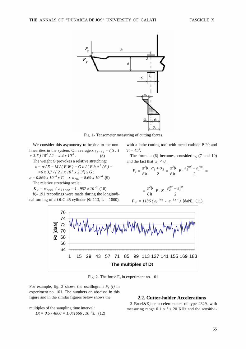
THE ANNALS OF “DUNAREA DE JOS” UNIVERSITY OF GALATI FASCICLE X
Fig. 1- Tensometer measuring of cutting forces
We consider this asymmetry to be due to the non-
linearities in the system. On average:ε I n r e g = ( 5 . 1 + 3.7 ) 10-3 / 2 = 4.4 x 10⁻³ . (8)
The weight G provokes a relative stretching: ε = σ / E = M / ( E W ) = G h / ( E b a 2 / 6 ) = =6 x 3,7 / ( 2.1 x 10 6 x 2.33) x G ;
ε = 0.869 x 10 -6 x G → ε real = 8.69 x 10 -6 .(9) The relative stretching scale:
K F = ε r e a l / ε I n r e g = 1 . 957 x 10 -3 .(10) b)- 191 recordings were made during the longitudi-
nal turning of a OLC 45 cylinder (Φ 113, L = 1000),
with a lathe cutting tool with metal carbide P 20 and ℜ = 45o.
The formula (6) becomes, considering (7 and 10) and the fact that ε1 < 0 :
=
−⋅⋅=
+⋅=
2E
h6ba
2h6baF
real1
real2
221
2
zεεσσ
2
KEh6ba inr
1inr2
2 εε −⋅⋅⋅=
F z = 1136 ( ε2 I n r - ε1
I n r ) [daN], (11)
64666870727476
1 15 29 43 57 71 85 99 113 127 141 155 169 183
The multiples of Dt
Fz [d
aN]
Fig. 2- The force Fz in experiment no. 101
For example, fig. 2 shows the oscillogram Fz (t) in experiment no. 101. The numbers on abscissa in this figure and in the similar figures below shows the multiples of the sampling time interval: Dt = 0.5 / 4800 = 1.041666 . 10 -4s. (12)
2.2. Cutter-holder Accelerations 3 Bruel&Kjaer accelerometers of type 4329, with
measuring range 0.1 < f < 20 KHz and the sensitivi-
55

FASCICLE X THE ANNALS OF “DUNAREA DE JOS” UNIVERSITY OF GALATI ___________________________________________________________________________ ties described below were mounted on a plate which was solidary with port-knife: - s = 12.5 mV/g, for accelerations on direction x (ax); - s = 11.5 mV/g, for accelerations on direction y (ay); - s = 13.5 mV/g, for accelerations on direction z (az). There exists the relation ship:
]/[.]/[
][ 2reala sma
s819g
sa
gmVsmVaa ⋅=⋅== ,(13)
where a [mV] is the input into Spider; therefore the PC recorded value is :
;.;. inry
realy
inrx
realx a8530aa7850a ⋅=⋅=
(14) inrz
realz a7270a ⋅= .
For example, recording no. 101 showed the oscilo-gram az
inr in fig. 3.
-0.015
-0.01
-0.005
0
0.005
0.01
1 9 17 25 33 41 49 57 65 73 81 89 97
The multiples of Dt
az [m
V]
Fig. 3- The acceleration az
inr in experiment no. 101
2.3. Tool Wear
After each passing the tool wear was measured with the help of a Brinell lens. The wear spot looked ir-regular (like a triangle), so the wear criterion VBmax was used.
The recordings which reached the limits of classes in table 1 were calculated by means of interpolation
3. Acknowledgement
This research was supported by a grant by Ministry of Education of Romania (Balan, 2002).
4. References Balan G ., The monitoring of a lathe using an artificial neural
network, Grant type A nr. 33 445, 2002, Theme 19, Cod CNCSIS 451
Colgan J, Chin H, Danai K, Hayashi SR (1994) On-line tool breakage detection in turning: a multi-sensor method, J Eng Ind 116:117–122
Crouse MS, Nowak RD, Baraniuk RG (1998) Wavelet-based statistical signal processing using hidden Markov models, IEEE Trans Signal Process 46(4):886–902
Sim WM, Dewes RC, Aspinwal AC (2000) A knowledge-based system for the selection of cutting tools and data for high speed machining of moulds/dies, Proceedings of the 33rd International Matador Conference, pp 119–125
Wang T, Meng C, Zhao G (1995) Research on intelligent moni-toring technology of machining process, International Confer-ence on Intelligent Manufacturing, Wuhan, China, pp 333–337
X. Q. Li, Y. S. Wong, A. Y. C. Nee (1997) Tool wear and chatter detection using the coherence function of two crossed accelera-tions, Int. J. Mech. Tools Manufact., Vol. 37, No. 4, pp. 425-437
56

THE ANNALS OF “DUNAREA DE JOS” UNIVERSITY OF GALATI FASCICLE X APPLIED MECHANICS, ISSN 1221-4612
2007
Buckling of composite panels with initial imperfections
Elena-Felicia Beznea, Ionel Chirică, Raluca Chirică “Dunarea de Jos” University of Galati
ABSTRACT In the paper, the buckling behaviour of laminated plates, with a pre-existing initial deformation and a central circular delamination, subjected to in-plane loading is treating. The plate is modelled as an orthotropic Mindlin plate. The analysis is carried out by using so layered shell elements, gap and coupling elements. By applying the finite element method, the plates with initial deformation (first modal shape of buckling) are studied. Numerical and experimental results for the critical buckling load are presented for several examples.
KEY WORDS: Imperfect Composite Plates, Buckling, FEM Analysis
1. Introduction In the paper, certain studies on buckling be-havior of the delaminated composite panels used in ship hull structures are presented. Both global and local sublaminate buckling deformation modes are predicted for rectangular plates of any thickness. The aim of the work presented in this paper is to analyze the influence of delamination on the changes in the buckling behaviour of structures with initial transversal deformations made of com-posite materials. This problem has been solved by using the finite element method. The work presented herein focuses on the buckling performance degradation of stability criti-cal structures having discrete zone of delamination. The plate is assumed to be thin relative to its span, such that buckling instead of compressive failure occurs. If an initial delamination exists, this delami-nation may close under the applied load. To prevent the two adjacent plies from penetrating, a simple contact model is used.
In this contact model, the normal stiffness of the interface is given a penalty value if the relative normal displacement between two adjacent plies is negative. The normal stiffness is zero if opening of the initial delamination occurs. The shear stiffness of the initial delamination zone is always taken equal to zero, so no friction is modelled. The aim of the work presented in this paper is to analyze the influence of delamination on the changes in the buckling behaviour of structures made of composite materials. This problem has been solved by using the finite element method. An orthotropic delamination model, describing mixed mode delaminating, by using COSMOS/M soft package, was applied. So, the damaged part of the structures and the undamaged part have been repre-sented by wellknown finite elements (layered shell elements). The influence of the position of circular delaminated zone on the critical buckling force was investigated.

FASCICLE X THE ANNALS OF “DUNAREA DE JOS” UNIVERSITY OF GALATI ___________________________________________________________________________ The delamination model has been developed by using the surface-to-surface contact option. In case of surface-to-surface contact, the FE meshes of adjacent plies do not need to be identical. The contact algorithm of COSMOS/M will determine which node of the so-called master surface is in contact with a given node on the slave surface. Hence, the user can define the interaction between the two surfaces.
- E-glass/epoxy: E1 = 46 GPa, E2 = 13 GPa, E3=13 GPa G12 = 5 GPa, G13 = 5 GPa, G23 = 4.6 GPa
12µ =0.3, =0.42, =0.3 23µ 13µ- UD layers: t1 = 0.59 mm; - Biaxial layers: t2 = 0.39 mm, modeled as two UD layers having thickness t2/2, at ±45°; - Lay-up is presented in Table 1. Numerical studies, non-linear analysis (large displacements), were performed with COSMOS/M code. For FEM analysis 3-node structural layered shell element (SHELL3L) were used.
In tests, the different layers are intentionally not connected to each other in circular regions. The condition is that the delaminated region does not grow. In COSMOS/M these regions were modeled by two layers of elements with coincident but sepa-rate nodes and section definitions to model offsets from the common reference plane. Thus, their de-formations are independent. At the boundary of the delamination zones the nodes of one row are con-nected to the corresponding nodes of the regular region by master slave node system.
Boundary conditions introduced were: - On x=0 edge, completely fixed; - On x=a edge, all DOF fixed, except x-translation; - On y=0, y=b edges, all DOF fixed, except x, y translations and z rotation.
Table 1 Plate lay-up
α t [mm] +450 0.195 -450 0.195 4 × 00 2.36 +450 0.195 -450 0.195 6 × 00 3.54 +450 0.195 -450 0.195 4 × 00 2.36 +450 0.195 -450 0.195
2. Numerical Modeling of the Delamination Region of the Clamped
Orthotropic Imperfect Plate Asymmetric sublaminate, generally would exhibit bending-stretching coupling resulting in pre-buckling out-out-plane displacements before any kind of buckling occurs. This is potentially a source of discrepancy between eigenvalue-based buckling predictions and actual mechanical behav-ior which is observable in tests and perhaps careful analyses in which end-loading versus out-of-plane displacements are predicted. The sublaminate may be modeled as a separate circular plate with clamped boundaries, for the local buckling. The loads applied to the sublaminate model are computed based upon the assumption that the in-plane loads acting on the plate section as a whole are the same throughout the entire plate, even in the delamination zone. The study of the influence of the position of delaminated region on buckling load of a clamped orthotropic plate, having initial transversal defor-mation, with 3 values of the magnitude, was made. The region was considered on the middle of the plate. The region was considered as the circular one. For each value of the initial transversal defor-mation magnitude, various position of the delami-nated region were considered along the thickness of the plate, considering different sublaminating lay-ers (from 1 to 11 layers).
The FEM model, composed of shell ele-ments, for geometric representation of a plate sized 320×320, thickness of 10 mm, having a circular delamination zone (with the diameters dx and dy), was made. The material used for the plate has the char-acteristics:
58
Figure 1: The plate model
The FEM model incorporates two sets of collocated shells in the delamination region, each representing an unsymmetric of a number of ni layers sublami-nate. The initial deformation of the plate has the shape of the first buckling mode of the clamped plate. Maximum initial deformation magnitude is considered as a rate from the thickness, t, that is wo = γ t. (1)In the analysis, for the rate γ the following values were chosen: 0.106, 0.32 and 0.96.

THE ANNALS OF “DUNAREA DE JOS” UNIVERSITY OF GALATI FASCICLE X __________________________________________________________________________
Fibers at -45°Fibers at +45° Fibers at 0° Figure 2: Fibers orientation in layers
Table 2: Lay-up and cases with position of delamination
Position of delamination L. No.
t [mm] α Case
1 Case
2 Case
3 Case
4 Case
5 Case
6 Case
7 Case
8 Case
9 Case 10
1 0.195 +450 1 L. 2 0.195 -450
2 L.
3 2.360 00
3L.
4 0.195 +450
4 L.
5 0.195 -450
5 L.
6 3.54 00
6 L.
7 0.195 +450
7 L.
8 0.195 -450
8 L.
9 2.36 00
9 L.
10 0.195 +450
10L.
11 0.195 -450
10 L. 9L.
8 L. 7L.
6 L. 5 L.
4 L. 3 L.
2 L. 1 L.
L.=layer
3. Numerical results for buckling force
The analysis of the buckling of the orthotropic delamination model, describing mixed mode de-laminating, by using COSMOS/M soft package, was applied. So, the damaged part of the structures and the undamaged part have been represented by layered shell elements. The influence of the posi-tion of circular delaminated zone on the critical buckling force was investigated.
In this contact model, the normal stiffness of
the interface is given a penalty value if the relative normal displacement between two adjacent plies is negative. The normal stiffness is zero if opening of the initial delamination occurs. The shear stiffness of the initial delamination zone is always taken equal to zero, so no friction is modelled.
In table 3, the values of the buckling stress [MPa], obtained for the 10 cases and the three val-ues of magnitude of the initial transversal deforma-tion are shown.
Table 3: Buckling stress [MPa]
w0Case
1 Case
2 Case
3 Case
4 Case
5 Case
6 Case
7 Case
8 Case
9 Case 10
1,06 86,6 86,1 79,8 79,2 78,7 78,7 79,2 79,8 86,1 86,5 3,2 95,2 94,7 87,7 87,2 86,6 86,5 87,2 87,8 94,6 95,2 9,6 105 104,6 99,9 99,5 99,2 99,1 99,5 99,9 104,7 105,
7
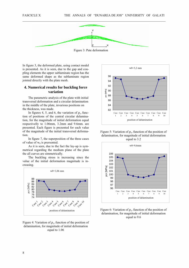
FASCICLE X THE ANNALS OF “DUNAREA DE JOS” UNIVERSITY OF GALATI ___________________________________________________________________________
Figure 3: Pate deformation
In figure 3, the deformed plate, using contact model is presented. As it is seen, due to the gap and cou-pling elements the upper sublaminate region has the same deformed shape as the sublaminate region jointed directly with the plate mesh.
4. Numerical results for buckling force variation
The parametric analysis of the plate with initial transversal deformation and a circular delamination in the middle of the plate, invarious positions on the thickness, was made. In figures 4, 5, and 6, the variation of pcr func-tion of positions of the central circular delamina-tion, for the magnitude of initial deformation equal respectivelly to 1.06mm, 3.2mm and 9.6mm. are presented. Each figure is prezented for each value of the magnitude of the initial transversal deforma-tion. In figure 7, the superposition of the three cases of value of w0 is prersented. As it is seen, due to the fact the lay-up is sym-metrical regarding the medium plane of the plate the all curves are simmetrically. The buckling stress is increasing since the value of the initial deformation magnitude is in-creasing.
w0=1,06 mm
7476788082848688
Case 1
Case 2
Case 3
Case 4
Case 5
Case 6
Case 7
Case 8
Case 9
Case 10
position of delamination
pcr [
MPa
]
Figure 4: Variation of pcr function of the position of delamination, for magnitude of initial deformation
equal to 1.06
w0=3,2 mm
82
84
86
88
90
92
94
96
Case1
Case2
Case3
Case4
Case5
Case6
Case7
Case8
Case9
Case10
position of delamination
pcr [
MP
a]
Figure 5: Variation of pcr function of the position of delamination, for magnitude of initial deformation
equal to 3.2
w0=9,6mm
96979899
100101102103104105106
Case1
Case2
Case3
Case4
Case5
Case6
Case7
Case8
Case9
Case10
position of delamination
pcr [
MP
a]
Figure 6: Variation of pcr function of the position of delamination, for magnitude of initial deformation
equal to 9.6
8
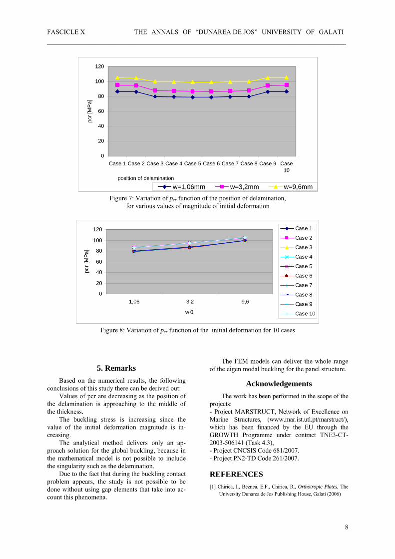
FASCICLE X THE ANNALS OF “DUNAREA DE JOS” UNIVERSITY OF GALATI ___________________________________________________________________________
0
20
40
60
80
100
120
Case 1 Case 2 Case 3 Case 4 Case 5 Case 6 Case 7 Case 8 Case 9 Case10
position of delamination
pcr [
MP
a]
w=1,06mm w=3,2mm w=9,6mm
Figure 7: Variation of pcr function of the position of delamination, for various values of magnitude of initial deformation
0
20
40
60
80
100
120
1,06 3,2 9,6
w 0
pcr [
MPa
]
Case 1
Case 2
Case 3
Case 4
Case 5
Case 6
Case 7
Case 8
Case 9
Case 10
Figure 8: Variation of pcr function of the initial deformation for 10 cases
5. Remarks Based on the numerical results, the following conclusions of this study there can be derived out: Values of pcr are decreasing as the position of the delamination is approaching to the middle of the thickness. The buckling stress is increasing since the value of the initial deformation magnitude is in-creasing. The analytical method delivers only an ap-proach solution for the global buckling, because in the mathematical model is not possible to include the singularity such as the delamination. Due to the fact that during the buckling contact problem appears, the study is not possible to be done without using gap elements that take into ac-count this phenomena.
The FEM models can deliver the whole range of the eigen modal buckling for the panel structure.
Acknowledgements The work has been performed in the scope of the projects: - Project MARSTRUCT, Network of Excellence on Marine Structures, (www.mar.ist.utl.pt/marstruct/), which has been financed by the EU through the GROWTH Programme under contract TNE3-CT-2003-506141 (Task 4.3), - Project CNCSIS Code 681/2007. - Project PN2-TD Code 261/2007.
REFERENCES [1] Chirica, I., Beznea, E.F., Chirica, R., Orthotropic Plates, The
University Dunarea de Jos Publishing House, Galati (2006)
8

FASCICLE X THE ANNALS OF “DUNAREA DE JOS” UNIVERSITY OF GALATI ___________________________________________________________________________ [2] Chirica, I., Beznea, E.F., Chirica, R., Boazu, D., Chirica, A.,
Buckling Behavior of the Delaminated Ship Hull Panels, Proceedings of The 12-th International Maritime Associa-tion of the Mediterranean Congress – IMAM, 2-6 sept. 2007, Varna, Bulgaria, pp. 161-166, vol. 1-Maritime Trans-portation, Ed. Taylor&Francis, ISBN 978-0-415-43725-7 (2007)
[3] Hayman, B., Defect and damage assessment for ships built in FRP sandwich, RINA Conference on High Speed Craft, Royal Institution of Naval Architects, London, UK, Novem-ber (2004)
[4] Kim, H., & Kedward, K.T., A Method for Modeling the Local and Global Buckling of Delaminated Composite Plates, Com-posite Structures 44, p. 43-53 (1999)
[5] Linde, P., Schulz, A. & Rust, W., Influence of modelling and solution methods on the FE-simulation of the post-buckling behaviour of stiffened aircraft fuselage panels, Composite Structures 73, pp.229–236 (2006).
8

THE ANNALS OF “DUNAREA DE JOS” UNIVERSITY OF GALATI FASCICLE X APPLIED MECHANICS, ISSN 1221-4612
2007
Torsional vibrations analysis of a container-ship hull model, made of composite materials
Raluca Chirică, Sorin Dumitru Muşat, Elena-Felicia Beznea “Dunarea de Jos” University of Galati
ABSTRACT In the paper, the torsional vibration of the ship is treated.Taking into account the thin-walled beam theory, the torsion behaviour analysis of simple open and closed section beam is presented. Finally, the torsion analysis of a ship hull container model, made of composite material, based on FEM analysis is presented.The work was made within the European Project FP6- MARSTRUCT, Network of Exce-lence on Marine Structures, which has been financed by the EU through the GROWTH Programme under contract TNE3-CT-2003-506141 (Task 4.3).
1. Introduction
Stimulated by the vast potential advantages provided by new composite materials, the anisotropic composite thin-walled beam structures are likely to play a crucial role in the construction of actual and future generation of high performance vehicles. The extensive research activities related to the thin-walled beams in the past have covered a broad range of domains such as aeroelastic tailoring, smart materials/structures as well as the theoretical issues prompted by the multitude of the unusual effects inherent in this kind of structures. It is more than sure that this research trend will continue and get intensified in the years ahead. Among the unusual effects of the composite thin-walled beam structures, those contributed from warping and warping restraint, transverse shear strain, 3-D strain effect, and non-uniformity of the transverse shear stiffness within the structure, have been identified to have significant influence on the prediction accuracy of the models. Due to the complex influence of these non-classical effects, it is vital to validate the related models. In fact, during the last two decades, a number of analytical models for thin-
walled beams have been proposed in specialized contexts and validated either numerically or experimentally. On the other hand, refined thin-walled beam theory originally developed in some papers has been extensively used for the study, among others, of dynamic response/structural feedback control and static ship hull elasticity. For these beam models, certain validation against the experimental and analytical predictions provided by other models of thin-walled beams is available in the literature. Moreover, the 3-D strain effect, the non-uniformity of contourwise shear stiffness has not been accounted for in the model. It is a well-known fact that the next generation of advanced water vehicles, in general, and the combat ships of the post-cold era, in particular, are likely to operate in more severe environmental conditions than in the past. In this connection, the dynamic elastic response of ship hulls to time-dependent external loading, such as waves and water explosive blast induced loads, is closely related to the level of the operational qualities of these water vehicles. In spite of the evident practical importance of the problem involving the determination of the dynamic elastic response of

FASCICLE X THE ANNALS OF “DUNAREA DE JOS” UNIVERSITY OF GALATI
ship hulls to time-dependent pressure pulses, there are very few works addressing this issue. The literature is especially devoted to the dynamic aeroelastic response that is quite void of such works. In (Marzocca, P., &all, 2001) the problem is considered in a comprehensive form, including the combination of various gusts and explosive blast loads. However, the structural model is still based on the 2-D cross-section. This article approaches the problem in an extended context in the sense that the aircraft wing is modeled as an anisotropic thin-walled beam and based on it, the elastic tailoring effects on the dynamic aeroelastic response are investigated. Special attention is given to the formulation of the problem and the solution methodology. It should be noted that due to the nonconservative nature of the problem, the classical modal analysis is not efficient for the solution.
2. State of the art in the thin-walled beam theory
In this chapter a brief literature review of thin-walled structures and an overview of bending and buckling of thin plates is presented together with the theories of torsion of thin-walled open sections.
2.1 General equations A thin-walled structure is defined as a structure that is made from thin plates joined along their edges. The plate thickness is small compared to other cross-sectional dimensions which are in turn often small compared to the overall length. There are several reasons why thin-walled structures must be given special consideration in their analysis and design. In a thin-walled beam the shear stresses and strains are much larger relative to those in a solid rectangular beam. When certain thin-walled structures are twisted there is a so-called warping of the cross-section and the Bernoulli hypothesis is violated. The term warping is defined as the out-of-plane distortion of the cross-section of a beam in the direction of its longitudinal axis. Thin-walled structures are also susceptible to local buckling if the in-plane stresses reach their critical values. If this happens, the geometry of the cross-section changes, in contrast to overall buckling where the cross-sectional form is retained, as in the case of a pin-ended column. However, if a thin-walled column is made sufficiently long it may suffer overall buckling before it buckles locally. This means that thin-walled structures must be designed against both local and overall buckling. Theory and experiments show that these two phenomena can interact and when this happens the buckling load can decrease below the values of the individual loads.
There is an extensive amount of literature dealing with the theory of thin-walled structures and it is beyond the scope of this thesis to review this literature to any larger extent. However, a brief review of some literature on the elastic buckling of thin-walled structures is given below. The membrane theory of plates was first studied by Euler (1766) and the flexural theory by Bernoulli (1789) and Navier (1823). The theory for combined membrane and flexural effects was developed by Kirchhoff (1877) and Saint-Venant (1883). At this state, the governing equation for thin isotropic plates loaded laterally with q per unit area and in-plane forces Nx, Nz and Nxz per unit length was
2
22
2
2
4
4
22
4
4
4
2
2
zwN
zxwN
xwNq
zw
zxw
xwD
zxzx∂∂
+∂∂
∂+
∂∂
+=
=⎥⎦
⎤⎢⎣
⎡
∂∂
+∂∂
∂+
∂∂
(1)
where w is the lateral deflection. At the turn of the twentieth century the equation governing the buckling of flat plates was available and it was known that it forms the basis of an eigenvalue problem. At that time it was not recognised that as the plate buckles the values of x, Nx and Nxz at a given point would vary because of the stretching of the plate. The next development which overcame this deficiency was due to Foppl (1907) who introduced the stress function Φ and paved the way for von Karman (1910) to derive the governing equations for perfectly flat plates
qzx
wzxz
wxx
wz
zw
zxw
xwD
+∂∂
∂∂∂Φ∂
−∂∂
∂Φ∂
+∂∂
∂Φ∂
=
=⎥⎦
⎤⎢⎣
⎡
∂∂
+∂∂
∂+
∂∂
22
2
2
2
2
2
2
2
2
4
4
22
4
4
4
2
2 (2)
⎥⎥⎦
⎤
⎢⎢⎣
⎡
∂∂
∂∂
−⎟⎟⎠
⎞⎜⎜⎝
⎛
∂∂∂
=
=∂
Φ∂+
∂∂Φ∂
++∂
Φ∂
2
2
2
222
4
4
22
4
4
4
2
zw
xw
zxwEt
zzxx (3)
These equations enabled the post-buckling behaviour of perfectly flat plates to be studied. The von Karman large-deflection equations for flat isotropic plates with in-plane loading were modified to account for anisotropy by Rostovtsev (1940) and later the effect of initial imperfections were included resulting in the following simultaneous equations:
( ) ( ) ( ) qzxwy
zxzwy
xxwy
zzwD
zxwH
xwD zx +
∂∂+∂
∂∂Φ∂
−∂
+∂∂
Φ∂+
∂+∂
∂Φ∂
=∂∂
+∂∂
∂+
∂∂ 22
2
2
2
2
2
2
2
2
4
4
22
4
4
4
22 (4)
64
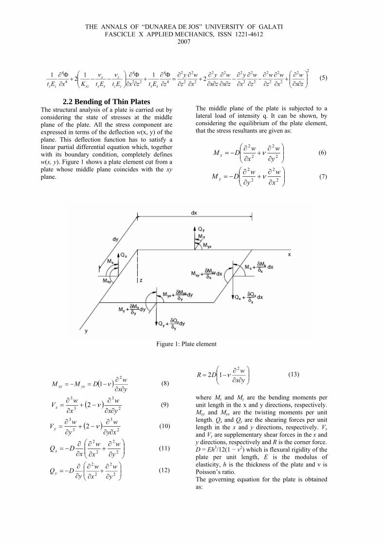
THE ANNALS OF “DUNAREA DE JOS” UNIVERSITY OF GALATI FASCICLE X APPLIED MECHANICS, ISSN 1221-4612
2007
22
2
2
2
2
2
2
2
222
2
2
2
2
4
4
22
4
4
4
21121⎟⎟⎠
⎞⎜⎜⎝
⎛
∂∂∂
+∂∂
∂∂
−∂∂
∂∂
−∂∂
∂∂∂
∂+
∂∂
∂∂
=∂
Φ∂+
∂∂Φ∂
⎟⎟⎠
⎞⎜⎜⎝
⎛−−+
∂Φ∂
zxw
xw
zw
zw
xy
zxw
zxy
xw
zy
zEtzxEtEtKxEt xxzz
z
xx
x
xzzz
νν (5)
2.2 Bending of Thin Plates
The structural analysis of a plate is carried out by considering the state of stresses at the middle plane of the plate. All the stress component are expressed in terms of the deflection w(x, y) of the plane. This deflection function has to satisfy a linear partial differential equation which, together with its boundary condition, completely defines w(x, y). Figure 1 shows a plate element cut from a plate whose middle plane coincides with the xy plane.
( )yx
wDMM yxxy ∂∂∂
−=−=2
1 ν (8)
( )2
3
3
3
2yxw
xwVx
∂∂∂
−+∂∂
= ν (9)
( )2
3
3
3
2xyw
ywVy
∂∂∂
−+∂∂
= ν (10)
⎟⎟⎠
⎞⎜⎜⎝
⎛
∂∂
+∂∂
∂∂
−=2
2
2
2
yw
xw
xDQx (11)
⎟⎟⎠
⎞⎜⎜⎝
⎛
∂∂
+∂∂
∂∂
−=2
2
2
2
yw
xw
yDQy (12)
The middle plane of the plate is subjected to a lateral load of intensity q. It can be shown, by considering the equilibrium of the plate element, that the stress resultants are given as:
⎟⎟⎠
⎞⎜⎜⎝
⎛
∂∂
+∂∂
−=2
2
2
2
yw
xwDM x ν (6)
⎟⎟⎠
⎞⎜⎜⎝
⎛
∂∂
+∂∂
−= 2
2
2
2
xw
ywDM y ν (7)
Figure 1: Plate element
⎟⎟⎠
⎞⎜⎜⎝
⎛∂∂
∂−=
yxwDR
2
12 ν (13)
where Mx and My are the bending moments per unit length in the x and y directions, respectively. Mxy and Myx are the twisting moments per unit length. Qx and Qy are the shearing forces per unit length in the x and y directions, respectively. Vx and Vy are supplementary shear forces in the x and y directions, respectively and R is the corner force. D = Eh3/12(1 − ν2) which is flexural rigidity of the plate per unit length, E is the modulus of elasticity, h is the thickness of the plate and ν is Poisson’s ratio. The governing equation for the plate is obtained as:

FASCICLE X THE ANNALS OF “DUNAREA DE JOS” UNIVERSITY OF GALATI
Dq
yw
yxw
xw
=∂∂
+∂∂
∂+
∂∂
4
4
22
4
4
4
2 (14)
Any plate problem should satisfy the governing equation (14) and boundary conditions of the plate.
2.3 Plate and Box Girder Analysis The high bending moments and shearing forces associated with the carrying of large loads over long spans, frequently necessitates the use of fabricated plate and box girders. In their simplest form, plate and box girders can be considered as an assemblage of webs and flanges. In order to reduce the self-weight of these girders and thus achieve economy, slender plate sections are employed. Hence local buckling and postbuckling reserve strength of plates are important design criteria. Flanges in a box girder and webs in plate and box girders are often reinforced with stiffeners to allow for efficient use of thin plates. The designer has to find a combination of plate thickness and stiffener spacing that will result in the most optimal section with reduced weight and fabrication cost. There are some difficulties that are usually encountered by designers of plated structures: • The engineer’s simple ‘plane sections remain plane’ theory of bending is no longer adequate, even for linear elastic analysis; • Non-linear elastic behaviour caused by the buckling of plates can be of great importance and must be allowed for; • Because of this complex non-linear elastic behaviour, and also because of stress concentration problems, some yielding may occur at loads which are quite low in relation to ultimate collapse loads. While such yielding may not be of great significance as regards rigidity and strength, it means that simple maximum stress criteria are no longer sufficient. • Because of the buckling problem in plates and stiffened panels, complete plastification is far from being realized at collapse. Hence simple plastic criteria are also not sufficient. • Complex interactions occur between flanges, webs and diaphragms and the pattern of this interaction can change as the level of load increases.
2.4 Torsion of Thin-Walled Open Sections
Thin-walled open cross-sections composed of slender plates are particularly susceptible to lateral torsional buckling, because the torsional rigidity of such cross-sections are low and so their resistance to torsional instability is limited. The analysis of lateral torsional buckling behaviour of beams is more complex than that of in-plane buckling behaviour of columns because
the lateral buckling problem is intrinsically three-dimensional. The problem is further complicated because the lateral (out-of-plane) deflection and twisting are coupled, so this coupling effect must be considered in the analysis 2.4.1 Uniform Torsion of Thin-Walled
Open Sections When an equal and opposite torque T is applied to the ends of a simply supported beam with a thin-walled open section, the twisting moment along the length of the members is constant and the beam is said to be under a uniform torsion. Under the action of the torque, warping of the cross-section will occur and plane sections of the cross-section no longer remain plane as a result of the uneven axial deformation that takes place over the entire cross-section. For the simply supported beam, in which warping of all the cross-sections is unrestrained, the applied torque is resisted only by shear stresses developed in the cross-section. These stresses act parallel to the edge of the component plates of the cross-section, as shown in Figure 2. The distribution of these shear stresses is the same for all thin-walled, open cross-sections. The magnitude of these shear stresses will be proportional to the distance from the midline of the component plate. These shear stresses are called Saint-Venant shear stresses and the associated torsion is referred to as Saint-Venant torsion, Tsv. The angle of twist γ over the length L caused by the Saint-Venant torsion is given by
GJT
Lsv=
γ (16)
where γ/L is the angle of twist per unit length, G is the shear modulus and J is the torsional constant of the cross-section.
Figure 2: Saint-Venant shear stress distribution in an I-section
The rate of twist is expressed as
GJT
zsv=
ddγ (17)
64

FASCICLE X THE ANNALS OF “DUNAREA DE JOS” UNIVERSITY OF GALATI
where z is the coordinate axis along the length of the beam. Equation (17) can be written as
z
GJTsv ddγ
= (18)
The Saint-Venant torsion expressed in Equation (18) is also referred to as uniform or pure torsion.
2.4.2 Non-Uniform Torsion of Thin-Walled, Open Sections
Consider a cantilever beam subjected to a torque applied at the free end. At the free end the cross-section is free to warp, so the applied torque is resisted only by Saint-Venant torsion. At the fixed end, however, warping is prevented. As a result, in addition to Saint-Venant torsion, there exists another type of torsion known as warping restraint torsion in the cross-section. If the cross-section is prevented from warping, axial strain and axial stresses must be induced in the cross-section, in addition to the shear stresses. These induced axial stresses are in self-balance because no external axial force is applied to the beam. The resultant of these axial stresses in the two flanges constitutes a pair of equal moments called the bi-moment, Bω, acting oppositely in each of the two planes of the flanges. The development of these bending moments, or bi-moments, in the flanges in the cross-section is shown in Figure 3. Since warping is prevented at the fixed end, the two flanges of the beam must bend in opposite directions as the cross-section rotates under the action of the applied torque. The bending of the flanges will thus induce bending moments Mf at the fixed end. The bending moment can be expressed in terms of the lateral displacement uf as
2
2
dzud
EIM fff = (19)
where E is the modulus of elasticity. If the moment of inertia of one flange about the y axis of the cross-section, and uf the lateral displacement of the flange. Associated with the bending moment in one flange is the shear force Vf given by
3
3
dd
dd
zu
EIz
MV f
ff
f −=−= (20)
The shear forces are present in both flanges of the I-section. They are equal in magnitude but act in opposite directions, as shown in Figure 4. This pair of shear forces constitute a couple acting on the cross-section. The resulting torsion, which is referred to as the warping restraint torsion or non-uniform torsion, is given by (21) hVT f=ω
where h is the distance between the lines of action of the shear forces. Equation (21) can be expressed as
Figure 3: Bending of flanges due to warping restraint at the fixed end.
3
3
3
32
2 dzdEC
dxdhEIT f
γγωω −=−= (22)
where
2
2hIC f=ω
(23)
is called the warping constant of the I-section. The warping constant is different for different cross-sections.
Figure 4: Moment and shear developed at the fixed-end cross-section of an I section
If warping is restrained, the applied twisting moment will be resisted by both Saint-Venant torsion and warping restraint torsion
ωTTT sv += (24) or
3
3
dd
dd
zEC
zGJT γγ
ω−= (25)
65

FASCICLE X THE ANNALS OF “DUNAREA DE JOS” UNIVERSITY OF GALATI
Equation (25) represents the internal twisting moment that will develop in the cross-section when the member is twisted. The first term represents the resistance of the cross-section to twisting and the second term represents the resistance of the cross-section to warping. Saint-Venant torsion is always present when a member is subjected to twisting and rotates. Warping restraint torsion will develop if a cross-section is prevented from warping when it is being twisted. 6. Analysis of the container ship model The torsion behaviour of a container ship model was made. The real ship has the following characteristics: - 1600 containers. - Length L=120 m, - Beam B=20 m, - Depth D=10 m. The dimensions of the all openings in the deck are: - length, l=30 m, - breadth, b=15 m. Due to the fact the container ship model is analised, the scale of the model is 1:50. So, the main characteristics of the analysed model are:
- Length L=2400 mm, - Beam B=400 mm, - Depth D=200 mm. A continuum opening in the deck was considered having the dimensions: - l= 600 mm, - b= 300 mm. The hull shape is a cilindrical one. The mechanical characteristics of the material are: E1=46 GPa, E2=13 GPa, G12=5 GPa, µ12=0.3, ρ= 1500 kg/m3. The ship model shell has the following thicknesses: - the outer shell: t=2mm - the deck plate: t=3mm To assure the indeformability of the hull in transversal direction, 13 bulkheads were placed. A natural vibrations analysis was made with COSMOS/M soft. The first 20 modal shapes were determined. The first 2 modal torsion vibrations are the modes 2 (43.55 Hz), 3(120,39 Hz) and 19 (275.95 Hz). The numerical results will be compared with the results obtained after the experimental tests.
In the figure 5, the geometry of the container ship model analysed is presented. As it is seen, the model has 3 parts: an open section in the middle part of the ship and closed section at the ends.
Figure 5: Container ship model
In figures 6, 7 and 8 the modal shapes resulted after the natural frequencies calculus are presented.
66
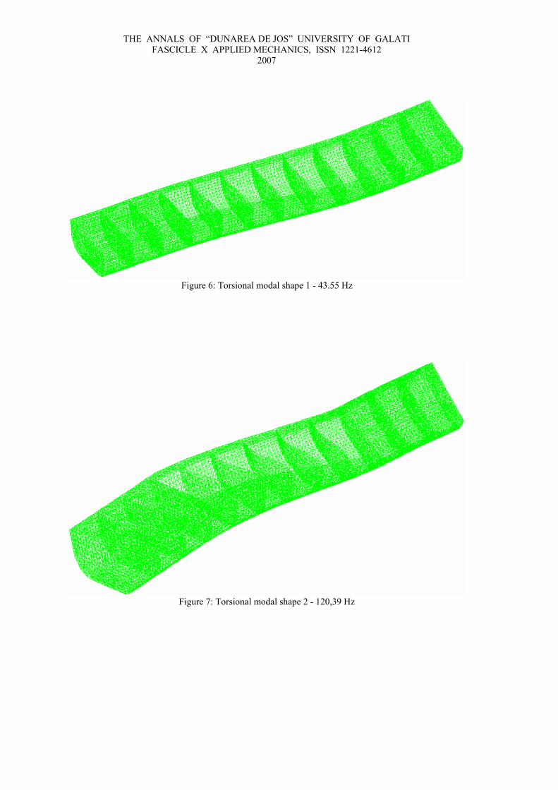
THE ANNALS OF “DUNAREA DE JOS” UNIVERSITY OF GALATI FASCICLE X APPLIED MECHANICS, ISSN 1221-4612
2007
Figure 6: Torsional modal shape 1 - 43.55 Hz
Figure 7: Torsional modal shape 2 - 120,39 Hz

THE ANNALS OF “DUNAREA DE JOS” UNIVERSITY OF GALATI FASCICLE X APPLIED MECHANICS, ISSN 1221-4612
2007
Figure 8: Torsional modal shape 3 - 275.95 Hz
Acknowledgements The work has been performed in the scope of the project MARSTRUCT, Network of Excellence on Marine Structures, (www.mar.ist.utl.pt/marstruct/), which has been financed by the EU through the GROWTH Programme under contract TNE3-CT-2003-506141 (Task 4.3). References 1. Martin Ålenius, 2003, Finite Element Modelling of Composite Bridge Stability, MSc Thesis Stockholm 2. Marzocca, P., Librescu, L., and Chiocchia, G., 2001, Aeroelastic Response of 2-D Lifting Surfaces to Gust and Arbitrary Explosive Loading
Signatures, International Journal of Impact Engineering, Vol. 25, pp. 41–65 3. Song, O. and Librescu, L., 1993, Free Vibration of Anisotropic Composite Thin-Walled Beams of Closed Cross-Section Contour, Journal of Sound and Vibration, Vol. 167, No. 1, pp. 129–147 4. Chirica, I., Beznea, E.F., 2004, Elasticitatea materialelor anizotrope, Editura Fundatiei Universitare Dunarea de Jos, Galati, ISBN 973-627-176-5 5. Chirica, I., Chirica, R., 2005, Structuri compozite cu pereti subtiri, Editura Didactica si Pedagogica, Bucuresti, ISBN 973-30-1270-X 6. Chirica, I., Beznea, E.F., Chirica, R., 2006, Placi compozite, Editura Fundatiei Universitare Dunarea de Jos, Galati, ISBN (10) 973-627-337-7; ISBN (13) 978-973-627-337-7.