Analog Communication Systems

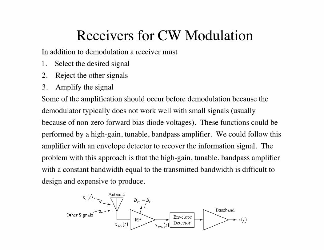
Receivers for CW ModulationIn addition to demodulation a receiver must1. Select the desired signal2. Reject the other signals3. Amplify the signalSome of the amplification should occur before demodulation because the demodulator typically does not work well with small signals (usuallybecause of non-zero forward bias diode voltages). These functions could be performed by a high-gain, tunable, bandpass amplifier. We could follow thisamplifier with an envelope detector to recover the information signal. The problem with this approach is that the high-gain, tunable, bandpass amplifier with a constant bandwidth equal to the transmitted bandwidth is difficult to design and expensive to produce.

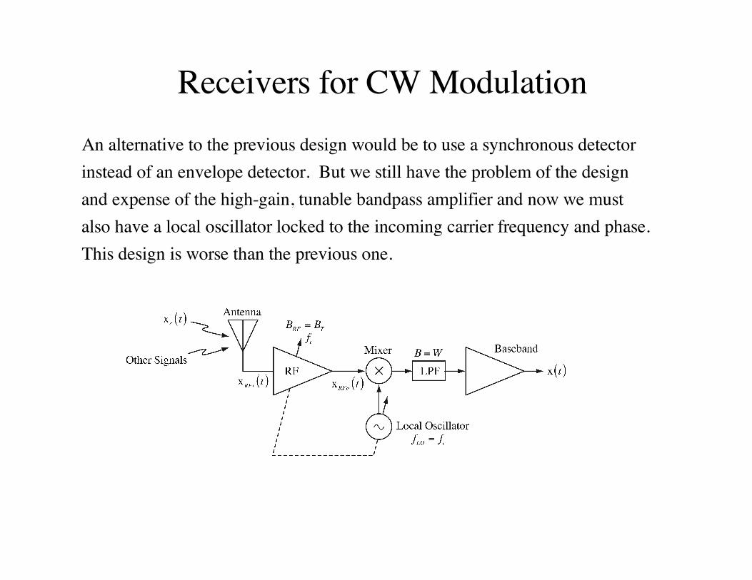
Receivers for CW ModulationAn alternative to the previous design would be to use a synchronous detectorinstead of an envelope detector. But we still have the problem of the designand expense of the high-gain, tunable bandpass amplifier and now we mustalso have a local oscillator locked to the incoming carrier frequency and phase. This design is worse than the previous one.

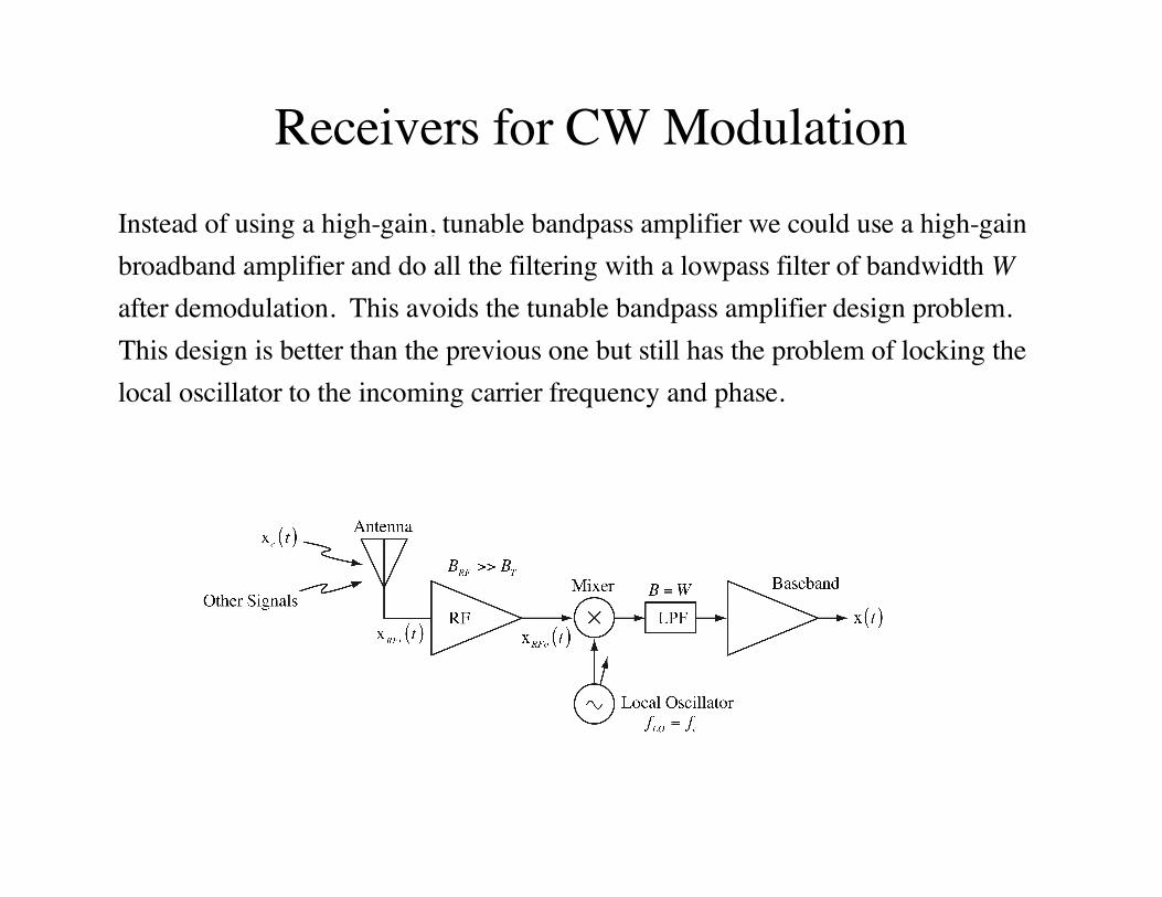
Receivers for CW ModulationInstead of using a high-gain, tunable bandpass amplifier we could use a high-gainbroadband amplifier and do all the filtering with a lowpass filter of bandwidth Wafter demodulation. This avoids the tunable bandpass amplifier design problem.This design is better than the previous one but still has the problem of locking thelocal oscillator to the incoming carrier frequency and phase.

Receivers for CW Modulation

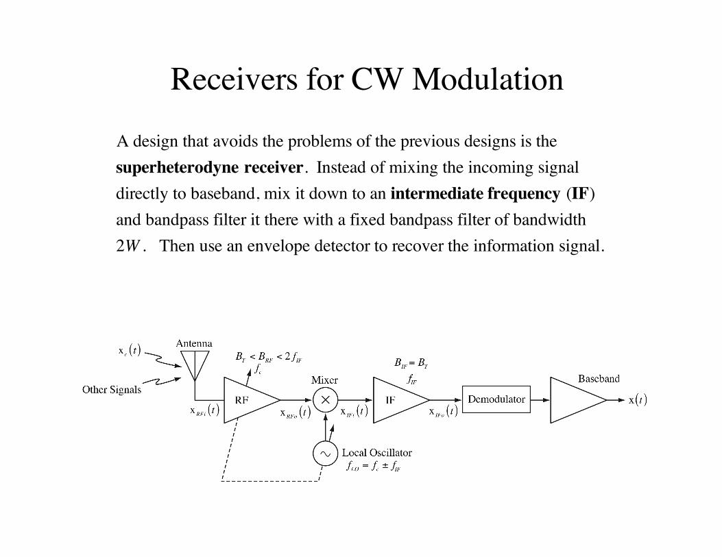
A design that avoids the problems of the previous designs is the superheterodyne receiver. Instead of mixing the incoming signaldirectly to baseband, mix it down to an intermediate frequency (IF) and bandpass filter it there with a fixed bandpass filter of bandwidth 2W . Then use an envelope detector to recover the information signal.

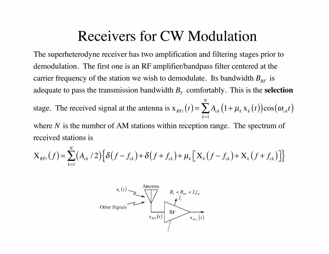
Receivers for CW ModulationThe superheterodyne receiver has two amplification and filtering stages prior to demodulation. The first one is an RF amplifier/bandpass filter centered at thecarrier frequency of the station we wish to demodulate. Its bandwidth BRF isadequate to pass the transmission bandwidth BT comfortably. This is the selection

stage. The received signal at the antenna is xRFi t( ) = Ack 1+ µk xk t( )( )cos ω ckt( )k=1

N

∑

where N is the number of AM stations within reception range. The spectrum of received stations is

XRFi f( ) = Ack / 2( ) δ f − fck( ) +δ f + fck( ) + µk Xk f − fck( ) + Xk f + fck( )⎡⎣ ⎤⎦{ }k=1

N

∑

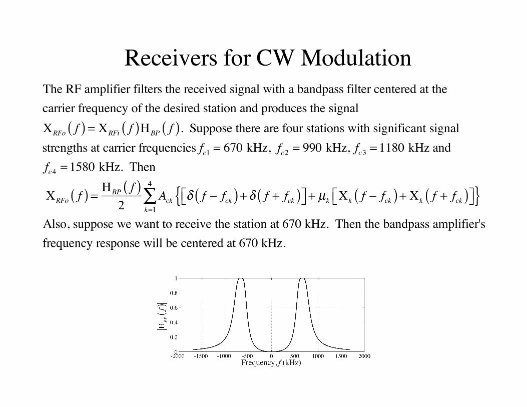
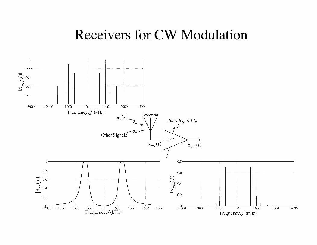
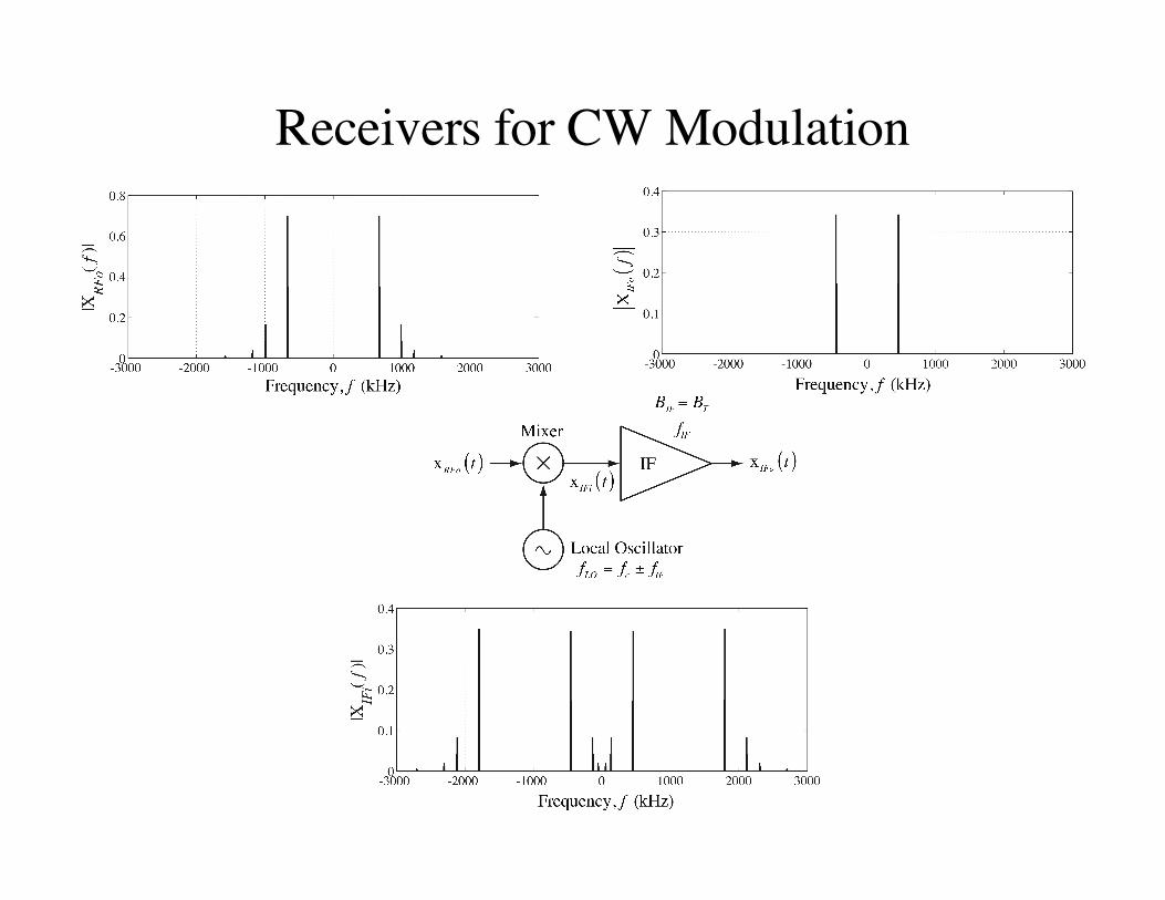
Receivers for CW ModulationThe RF amplifier filters the received signal with a bandpass filter centered at thecarrier frequency of the desired station and produces the signal XRFo f( ) = XRFi f( )HBP f( ). Suppose there are four stations with significant signalstrengths at carrier frequencies fc1 = 670 kHz, fc2 = 990 kHz, fc3 = 1180 kHz and fc4 = 1580 kHz. Then

XRFo f( ) = HBP f( )2

Ack δ f − fck( ) +δ f + fck( )⎡⎣ ⎤⎦ + µk Xk f − fck( ) + Xk f + fck( )⎡⎣ ⎤⎦{ }k=1

4

∑Also, suppose we want to receive the station at 670 kHz. Then the bandpass amplifier'sfrequency response will be centered at 670 kHz.

Receivers for CW Modulation

Receivers for CW Modulation

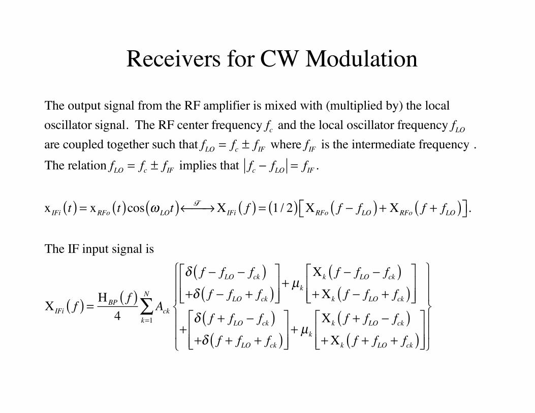
The output signal from the RF amplifier is mixed with (multiplied by) the local oscillator signal. The RF center frequency fc and the local oscillator frequency fLO are coupled together such that fLO = fc ± fIF where fIF is the intermediate frequency . The relation fLO = fc ± fIF implies that fc − fLO = fIF .

x IFi t( ) = xRFo t( )cos ω LOt( ) F← →⎯ XIFi f( ) = 1 / 2( ) XRFo f − fLO( ) + XRFo f + fLO( )⎡⎣ ⎤⎦.

The IF input signal is

XIFi f( ) = HBP f( )4

Ack

δ f − fLO − fck( )+δ f − fLO + fck( )⎡

⎣⎢⎢

⎤

⎦⎥⎥+ µk

Xk f − fLO − fck( )+Xk f − fLO + fck( )⎡

⎣⎢⎢

⎤

⎦⎥⎥

+δ f + fLO − fck( )+δ f + fLO + fck( )⎡

⎣⎢⎢

⎤

⎦⎥⎥+ µk

Xk f + fLO − fck( )+Xk f + fLO + fck( )⎡

⎣⎢⎢

⎤

⎦⎥⎥

⎧

⎨

⎪⎪

⎩

⎪⎪

⎫

⎬

⎪⎪

⎭

⎪⎪

k=1

N

∑

Receivers for CW Modulation

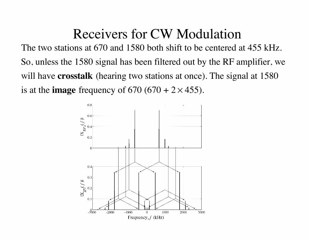
Receivers for CW ModulationThe two stations at 670 and 1580 both shift to be centered at 455 kHz. So, unless the 1580 signal has been filtered out by the RF amplifier, we will have crosstalk (hearing two stations at once). The signal at 1580is at the image frequency of 670 (670 + 2 × 455).

Receivers for CW Modulation

There are several parameters or "figures of merit" for receivers that are in common use.

Sensitivity - The minimum input voltage necessary to produce the specified signal- to-noise ratio S/N( )at the output of the IF section.Dynamic Range - The ratio of the maximum input signal strength the receiver can handle without significant distortion to the minimum signal strength at which it can meet the S/N requirementSelectivity - A measure of the ability of a radio receiver to select a particular frequency or particular band of frequencies and reject all unwanted frequenciesNoise Figure - The ratio of the S/N at the input to the S/N at the output, usually expressed in dBImage Rejection - The ratio of the response of the RF bandpass filter at the carrier frequency to its response at the image frequency, usually expressed in dB

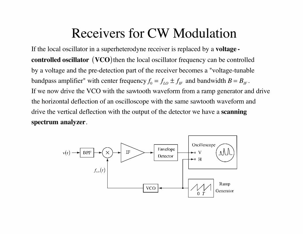
Receivers for CW ModulationIf the local oscillator in a superheterodyne receiver is replaced by a voltage -controlled oscillator VCO( ) then the local oscillator frequency can be controlled by a voltage and the pre-detection part of the receiver becomes a "voltage-tunablebandpass amplifier" with center frequency f0 = fLO ± fIF and bandwidth B = BIF .If we now drive the VCO with the sawtooth waveform from a ramp generator and drive the horizontal deflection of an oscilloscope with the same sawtooth waveform and drive the vertical deflection with the output of the detector we have a scanning spectrum analyzer.

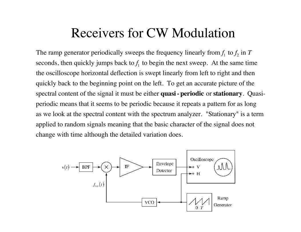
Receivers for CW ModulationThe ramp generator periodically sweeps the frequency linearly from f1 to f2 in T seconds, then quickly jumps back to f1 to begin the next sweep. At the same timethe oscilloscope horizontal deflection is swept linearly from left to right and then quickly back to the beginning point on the left. To get an accurate picture of thespectral content of the signal it must be either quasi - periodic or stationary. Quasi-periodic means that it seems to be periodic because it repeats a pattern for as longas we look at the spectral content with the spectrum analyzer. "Stationary" is a termapplied to random signals meaning that the basic character of the signal does notchange with time although the detailed variation does.

Multiplexing Systems

Multiplexing is the sending of multiple messages over the samecommunication channel. There are three basic types of multiplexing systems, frequency-division multiplexing (FDM), time-division multiplexing (TDM) and code-division multiplexing (CDM).

Multiplexing Systems

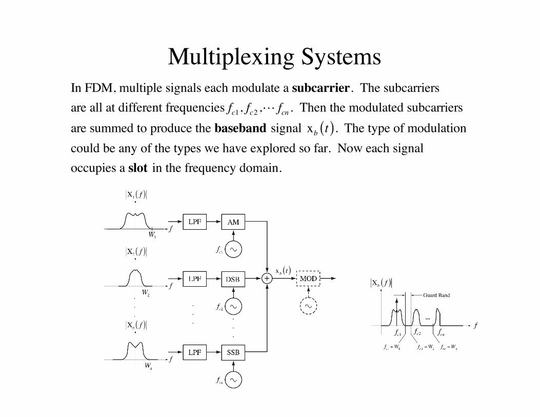
In FDM, multiple signals each modulate a subcarrier. The subcarriersare all at different frequencies fc1, fc2 , fcn . Then the modulated subcarriers are summed to produce the baseband signal xb t( ). The type of modulationcould be any of the types we have explored so far. Now each signal occupies a slot in the frequency domain.

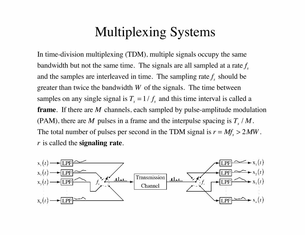
Multiplexing SystemsIn time-division multiplexing (TDM), multiple signals occupy the samebandwidth but not the same time. The signals are all sampled at a rate fsand the samples are interleaved in time. The sampling rate fs should be greater than twice the bandwidth W of the signals. The time betweensamples on any single signal is Ts = 1 / fs and this time interval is called a frame. If there are M channels, each sampled by pulse-amplitude modulation(PAM), there are M pulses in a frame and the interpulse spacing is Ts / M .The total number of pulses per second in the TDM signal is r = Mfs > 2MW .r is called the signaling rate.

Multiplexing Systems

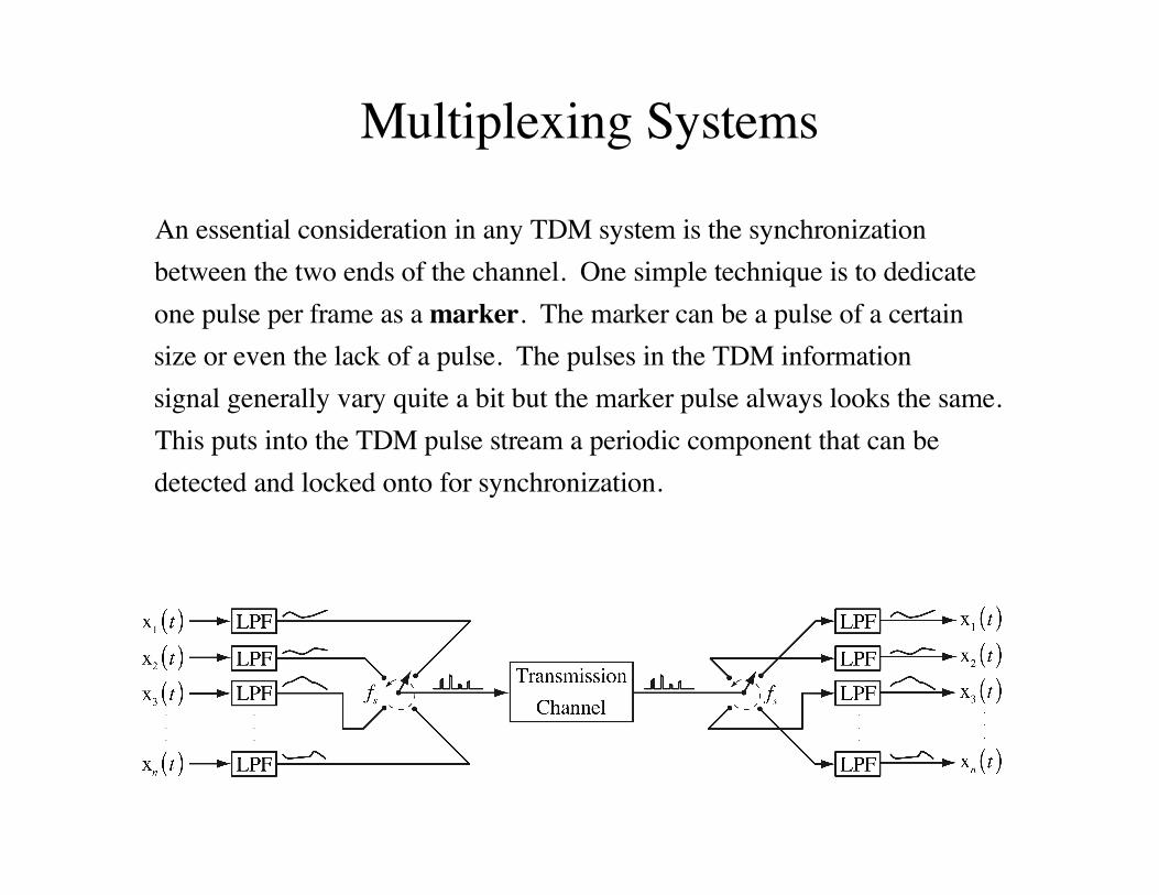
An essential consideration in any TDM system is the synchronizationbetween the two ends of the channel. One simple technique is to dedicateone pulse per frame as a marker. The marker can be a pulse of a certain size or even the lack of a pulse. The pulses in the TDM information signal generally vary quite a bit but the marker pulse always looks the same.This puts into the TDM pulse stream a periodic component that can be detected and locked onto for synchronization.

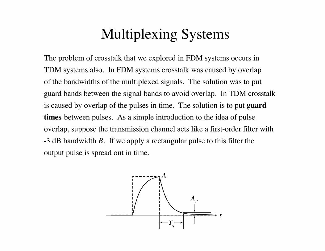
Multiplexing SystemsThe problem of crosstalk that we explored in FDM systems occurs in TDM systems also. In FDM systems crosstalk was caused by overlapof the bandwidths of the multiplexed signals. The solution was to putguard bands between the signal bands to avoid overlap. In TDM crosstalk is caused by overlap of the pulses in time. The solution is to put guard times between pulses. As a simple introduction to the idea of pulseoverlap, suppose the transmission channel acts like a first-order filter with-3 dB bandwidth B. If we apply a rectangular pulse to this filter the output pulse is spread out in time.

Multiplexing Systems

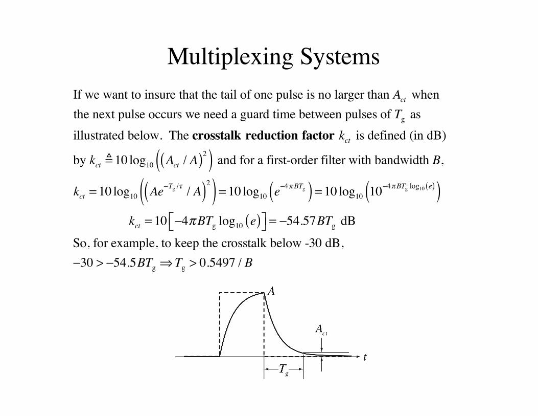
If we want to insure that the tail of one pulse is no larger than Act whenthe next pulse occurs we need a guard time between pulses of Tg as illustrated below. The crosstalk reduction factor kct is defined (in dB)

by kct 10 log10 Act / A( )2( ) and for a first-order filter with bandwidth B,

kct = 10 log10 Ae−Tg /τ / A( )2( ) = 10 log10 e−4πBTg( ) = 10 log10 10−4πBTg log10 e( )( ) kct = 10 −4πBTg log10 e( )⎡⎣ ⎤⎦ = −54.57BTg dB

So, for example, to keep the crosstalk below -30 dB, −30 > −54.5BTg ⇒Tg > 0.5497 / B

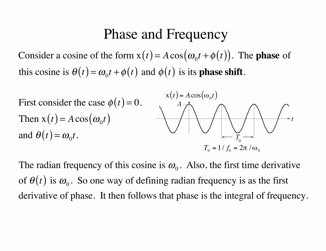
Phase and FrequencyConsider a cosine of the form x t( ) = Acos ω0t +φ t( )( ). The phase ofthis cosine is θ t( ) =ω0t +φ t( ) and φ t( ) is its phase shift.

First consider the case φ t( ) = 0. Then x t( ) = Acos ω0t( ) and θ t( ) =ω0t.

The radian frequency of this cosine is ω0 . Also, the first time derivative of θ t( ) is ω0 . So one way of defining radian frequency is as the first derivative of phase. It then follows that phase is the integral of frequency.

t

0T

Ax t( ) = Acos 0t( )

T0 = 1 / f0 = 2 / 0

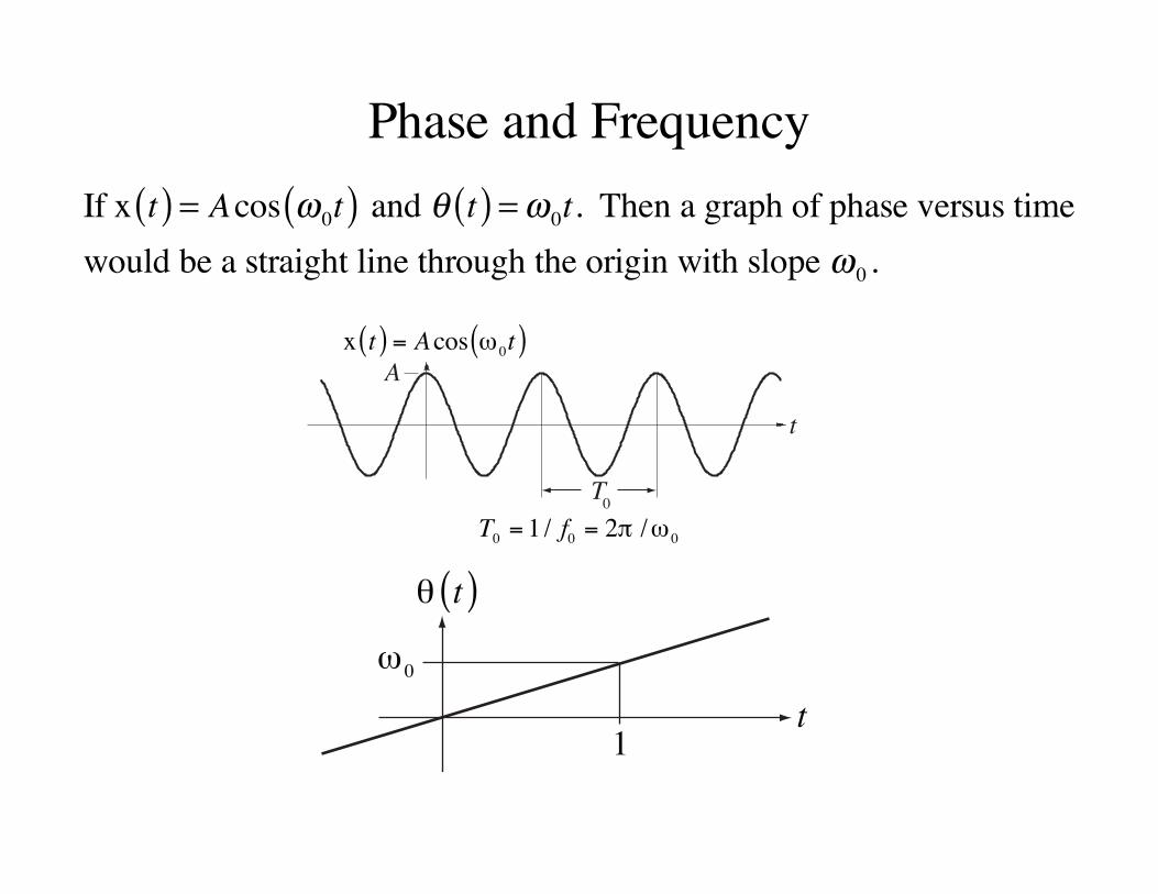
Phase and FrequencyIf x t( ) = Acos ω0t( ) and θ t( ) =ω0t. Then a graph of phase versus timewould be a straight line through the origin with slope ω0 .

t

0T

Ax t( ) = Acos 0t( )

T0 = 1 / f0 = 2 / 0

t

! t( )

1

" 0

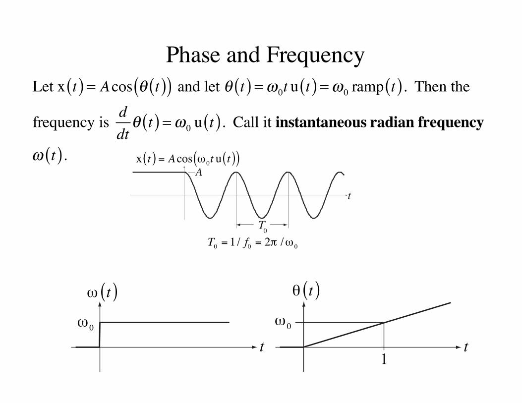
Phase and FrequencyLet x t( ) = Acos θ t( )( ) and let θ t( ) =ω0t u t( ) =ω0 ramp t( ). Then the

frequency is ddtθ t( ) =ω0 u t( ). Call it instantaneous radian frequency

ω t( ).

t

0T

A

T0 = 1 / f0 = 2 / 0

x t( ) = Acos 0t u t( )( )

t

! t( )

1

" 0

t" 0

" t( )

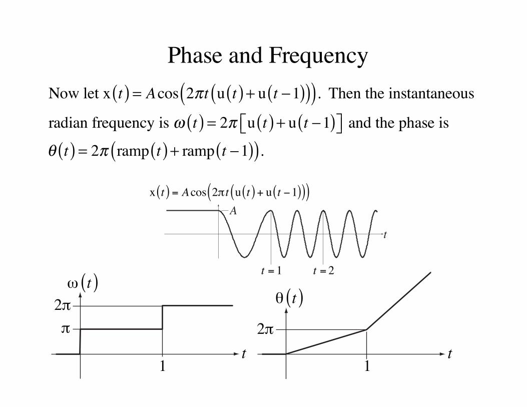
Phase and FrequencyNow let x t( ) = Acos 2πt u t( ) + u t −1( )( )( ). Then the instantaneous

radian frequency is ω t( ) = 2π u t( ) + u t −1( )⎡⎣ ⎤⎦ and the phase is

θ t( ) = 2π ramp t( ) + ramp t −1( )( ).

t11 t

! t( )" t( )

#2#

2#

t

A

t = 1 t = 2

x t( ) = Acos 2 t u t( ) + u t 1( )( )( )

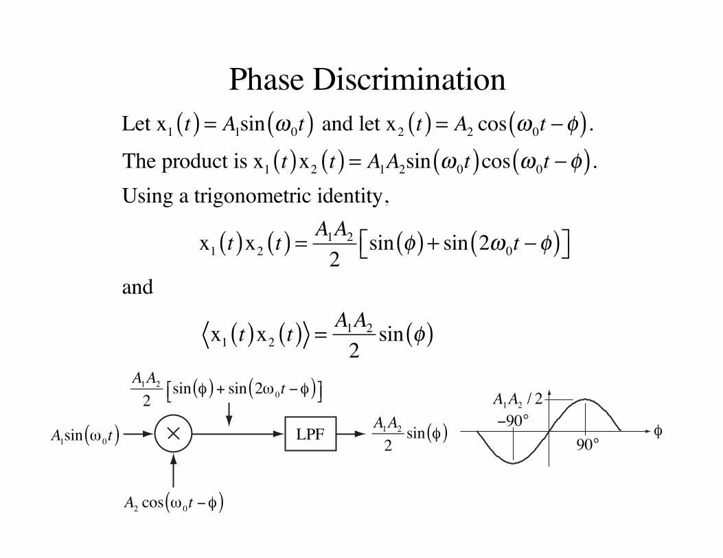
Phase DiscriminationLet x1 t( ) = A1sin ω0t( ) and let x2 t( ) = A2 cos ω0t −φ( ). The product is x1 t( )x2 t( ) = A1A2sin ω0t( )cos ω0t −φ( ).Using a trigonometric identity,

x1 t( )x2 t( ) = A1A2

2sin φ( ) + sin 2ω0t −φ( )⎡⎣ ⎤⎦

and

x1 t( )x2 t( ) = A1A2

2sin φ( )

LPFA1sin ! 0t( )

A2 cos ! 0t "#( )

A1A22 sin #( ) + sin 2! 0t "#( )$% &'

A1A22 sin #( )

A1A2 / 2

90°90°

Voltage-Controlled Oscillators

A voltage - controlled oscillator (VCO) is a device that accepts an analog voltage as its input and produces a periodic waveformwhose fundamental frequency depends on that voltage. Anothercommon name for a VCO is "voltage-to-frequency converter". The waveform is typically either a sinusoid or a rectangular wave. A VCO has a free-running frequency fv. When the input analogvoltage is zero, the fundamental frequency of the VCO output signalis fv. The output frequency of the VCO is fVCO = fv + Kv vin whereKv is a gain constant with units of Hz/V.

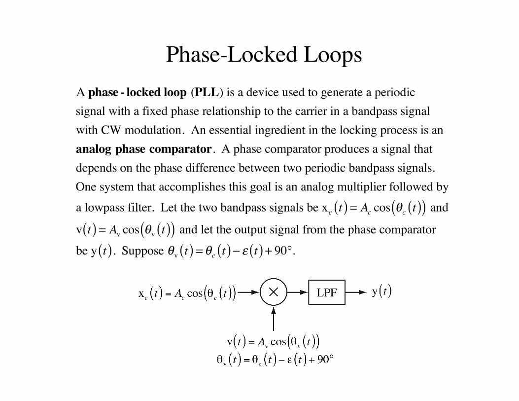
Phase-Locked LoopsA phase - locked loop (PLL) is a device used to generate a periodicsignal with a fixed phase relationship to the carrier in a bandpass signal with CW modulation. An essential ingredient in the locking process is an analog phase comparator. A phase comparator produces a signal that depends on the phase difference between two periodic bandpass signals. One system that accomplishes this goal is an analog multiplier followed by a lowpass filter. Let the two bandpass signals be xc t( ) = Ac cos θc t( )( ) and

v t( ) = Av cos θv t( )( ) and let the output signal from the phase comparator be y t( ). Suppose θv t( ) = θc t( )− ε t( ) + 90°.

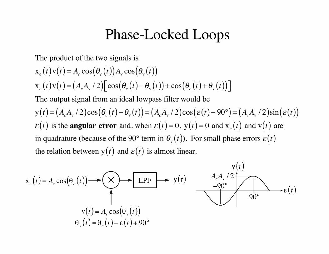
Phase-Locked LoopsThe product of the two signals is xc t( )v t( ) = Ac cos θc t( )( )Av cos θv t( )( )xc t( )v t( ) = AcAv / 2( ) cos θc t( )−θv t( )( ) + cos θc t( ) +θv t( )( )⎡⎣ ⎤⎦The output signal from an ideal lowpass filter would bey t( ) = AcAv / 2( )cos θc t( )−θv t( )( ) = AcAv / 2( )cos ε t( )− 90°( ) = AcAv / 2( )sin ε t( )( )ε t( ) is the angular error and, when ε t( ) = 0, y t( ) = 0 and xc t( ) and v t( ) arein quadrature (because of the 90° term in θv t( )). For small phase errors ε t( )the relation between y t( ) and ε t( ) is almost linear.

Phase-Locked Loops

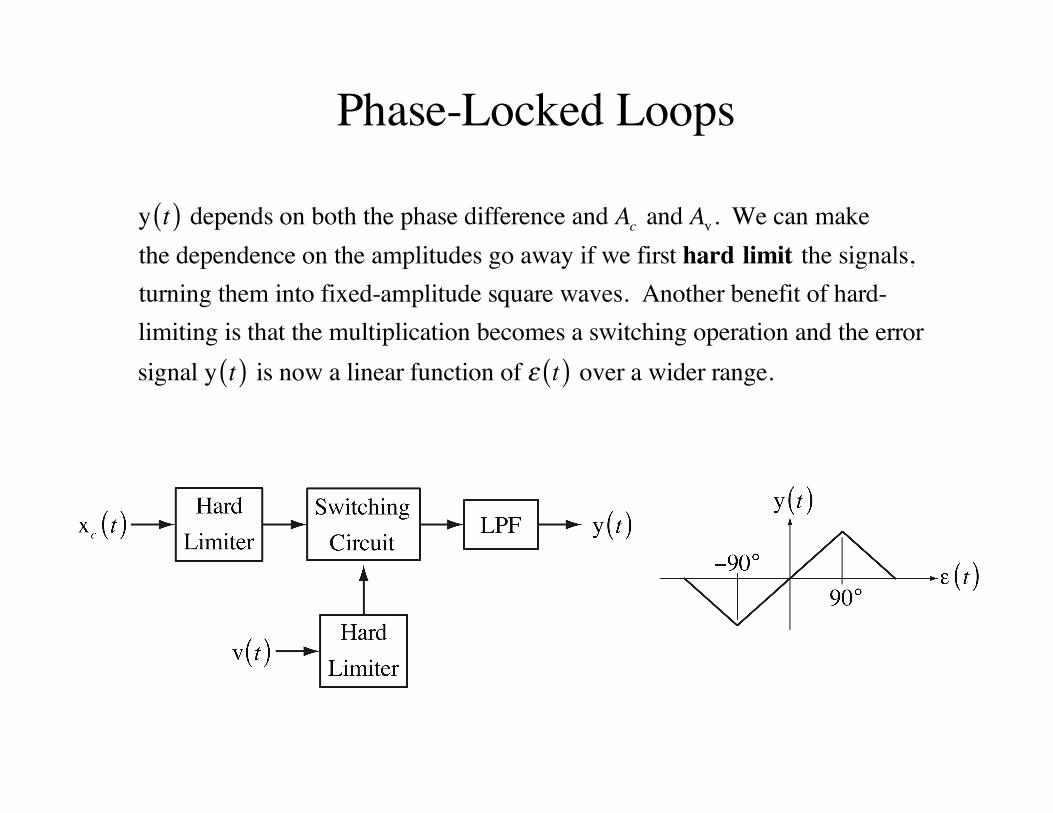
y t( ) depends on both the phase difference and Ac and Av. We can makethe dependence on the amplitudes go away if we first hard limit the signals, turning them into fixed-amplitude square waves. Another benefit of hard-limiting is that the multiplication becomes a switching operation and the error signal y t( ) is now a linear function of ε t( ) over a wider range.

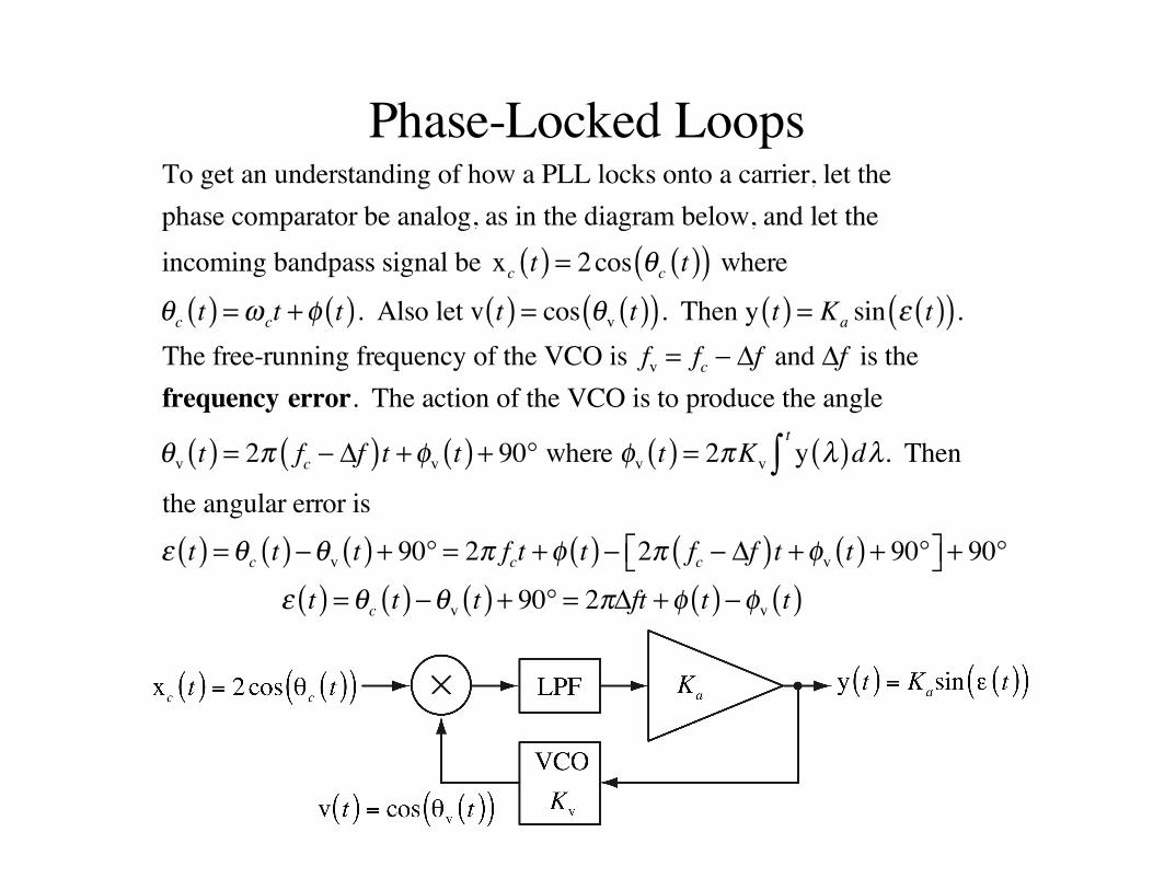
Phase-Locked LoopsTo get an understanding of how a PLL locks onto a carrier, let thephase comparator be analog, as in the diagram below, and let theincoming bandpass signal be xc t( ) = 2cos θc t( )( ) where

θc t( ) =ω ct +φ t( ). Also let v t( ) = cos θv t( )( ). Then y t( ) = Ka sin ε t( )( ).The free-running frequency of the VCO is fv = fc − Δf and Δf is the frequency error. The action of the VCO is to produce the angle

θv t( ) = 2π fc − Δf( )t +φv t( ) + 90° where φv t( ) = 2πKv y λ( )dλt

∫ . Then

the angular error is

ε t( ) = θc t( )−θv t( ) + 90° = 2π fct +φ t( )− 2π fc − Δf( )t +φv t( ) + 90°⎡⎣ ⎤⎦ + 90°

ε t( ) = θc t( )−θv t( ) + 90° = 2πΔft +φ t( )−φv t( )

Phase-Locked Loops

From the previous slide ε t( ) = θc t( )−θv t( ) + 90° = 2πΔft +φ t( )− φv t( )

2πKv y λ( )dλt

∫

Differentiating with respect to time, ε t( ) = 2πΔf + φ t( )− 2πKv y t( )

Ka sin ε t( )( )

ε t( ) + 2πKvKa sin ε t( )( ) = 2πΔf + φ t( )Let KvKa = K , the loop gain. Then ε t( ) + 2πK sin ε t( )( ) = 2πΔf + φ t( )This is a non-linear differential equation and cannot be solved in general for an arbitrary φ t( ). But consider the special case of φ t( ) = φ0 ,

a constant. Then φ t( ) = 0 and ε t( )

2πK+ sin ε t( )( ) = Δf / K . When the loop

is locked, ε t( ) is a constant ε ss , ε t( ) = 0, ε ss = sin−1 Δf / K( ) and

y t( ) = yss = Ka sin sin−1 Δf / K( )( ) = Δf / Kv

Phase-Locked Loops

In steady state, y t( ) = yss = Δf / Kv and vss t( ) = cos ω ct +φ0 − ε ss + 90°( ).The steady-state angular error ε ss = sin−1 Δf / K( ) will be small if the loop gain K is big. When Δf / K >1, the differential equation

ε t( )

2πK+ sin ε t( )( ) = Δf / K

does not have a steady-state solution because there is no real-valued solution of ε ss = sin−1 Δf / K( ). Therefore a lock-in condition is that Δf / K ≤1. At lock-in when ε ss is small the differential equation

becomes ε t( )

2πK+ ε t( ) ≅ Δf / K , a linear first-order equation with the

well-known solution form ε t( ) = ε t0( )e−2πK t−t0( ) , t ≥ t0 . So the responseof the PLL to sudden changes in input frequency is to approach steady

state on a time constant of 12πK

.

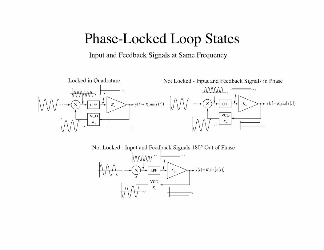
Phase-Locked Loop StatesInput and Feedback Signals at Same Frequency

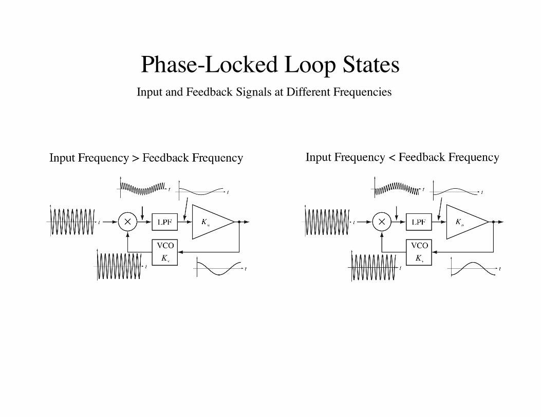
Phase-Locked Loop StatesInput and Feedback Signals at Different Frequencies

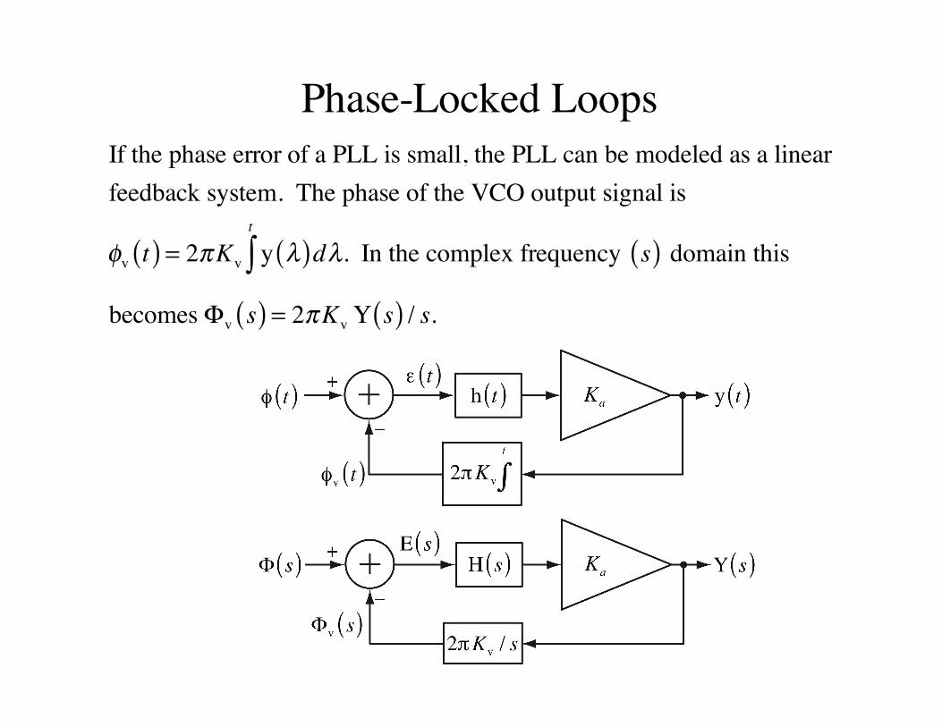
Phase-Locked LoopsIf the phase error of a PLL is small, the PLL can be modeled as a linearfeedback system. The phase of the VCO output signal is

φv t( ) = 2πKv y λ( )dλt

∫ . In the complex frequency s( ) domain this

becomes Φv s( ) = 2πKv Y s( ) / s.

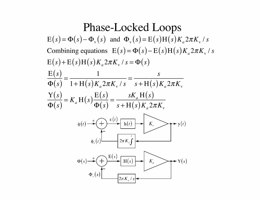
Phase-Locked LoopsE s( ) = Φ s( )− Φv s( ) and Φv s( ) = E s( )H s( )Ka2πKv / sCombining equations E s( ) = Φ s( )− E s( )H s( )Ka2πKv / sE s( ) + E s( )H s( )Ka2πKv / s = Φ s( )E s( )Φ s( ) =

11+ H s( )Ka2πKv / s

= ss + H s( )Ka2πKv

Y s( )Φ s( ) = Ka H s( ) E s( )

Φ s( ) =sKa H s( )

s + H s( )Ka2πKv

Phase-Locked Loops

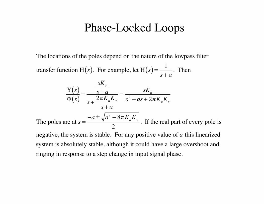
The locations of the poles depend on the nature of the lowpass filter

transfer function H s( ). For example, let H s( ) = 1s + a

. Then

Y s( )Φ s( ) =

sKa

s + as + 2πKaKv

s + a

= sKa

s2 + as + 2πKaKv

The poles are at s =−a ± a2 − 8πKaKv

2. If the real part of every pole is

negative, the system is stable. For any positive value of a this linearized system is absolutely stable, although it could have a large overshoot and ringing in response to a step change in input signal phase.

Phase-Locked Loops

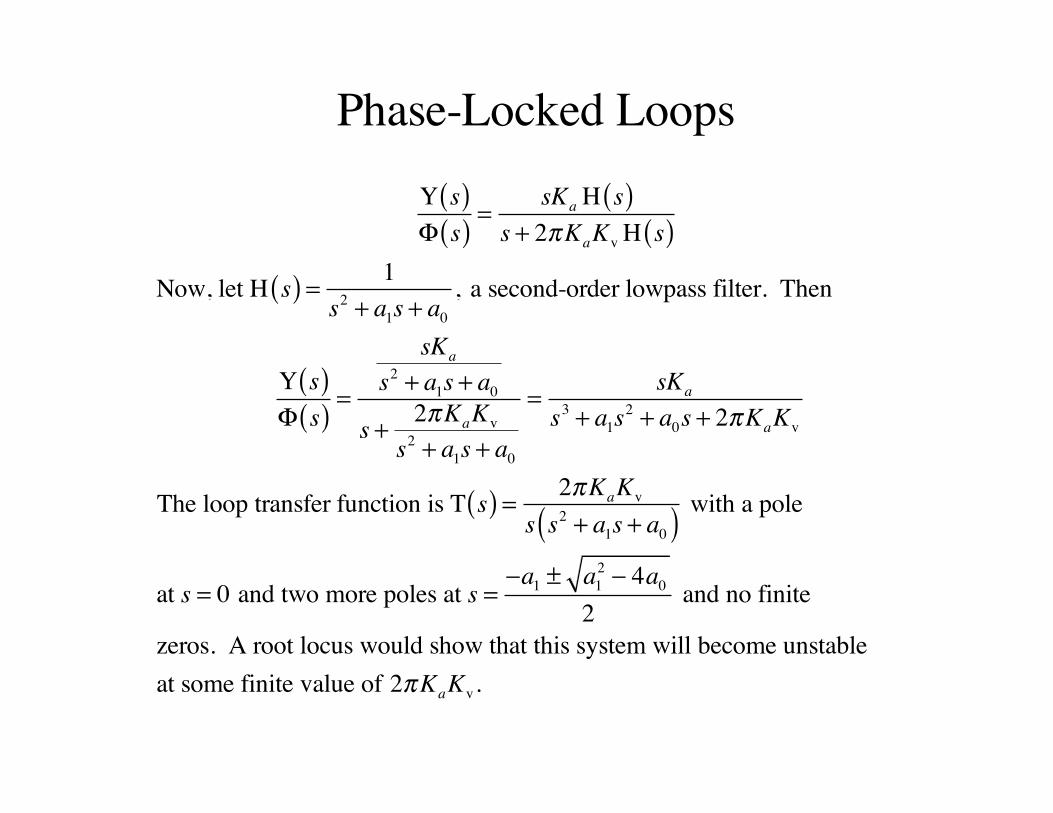
Y s( )Φ s( ) =

sKa H s( )s + 2πKaKv H s( )

Now, let H s( ) = 1s2 + a1s + a0

, a second-order lowpass filter. Then

Y s( )Φ s( ) =

sKa

s2 + a1s + a0

s + 2πKaKv

s2 + a1s + a0

= sKa

s3 + a1s2 + a0s + 2πKaKv

The loop transfer function is T s( ) = 2πKaKv

s s2 + a1s + a0( ) with a pole

at s = 0 and two more poles at s =−a1 ± a1

2 − 4a0

2 and no finite

zeros. A root locus would show that this system will become unstable at some finite value of 2πKaKv.

Phase-Locked Loops

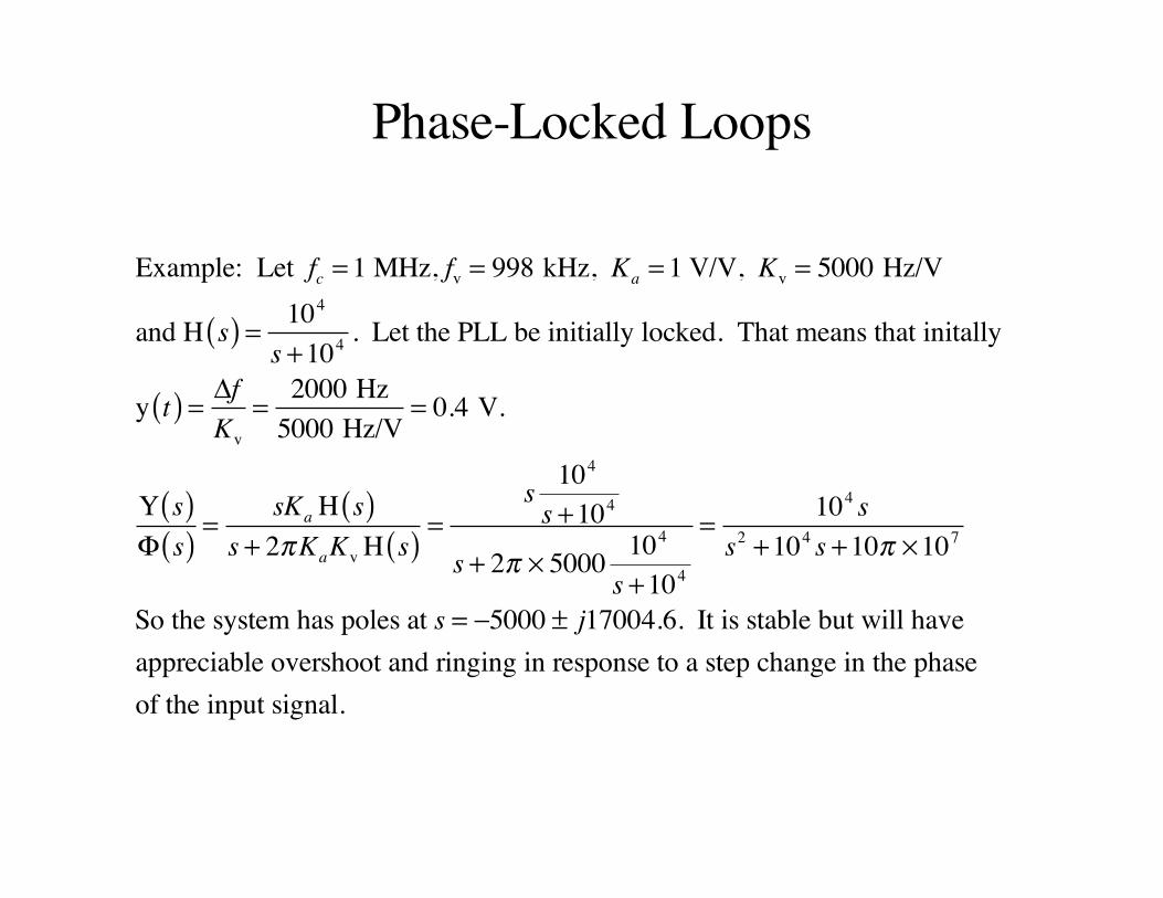
Example: Let fc = 1 MHz, fv = 998 kHz, Ka = 1 V/V, Kv = 5000 Hz/V

and H s( ) = 104

s +104 . Let the PLL be initially locked. That means that initally

y t( ) = ΔfKv

= 2000 Hz5000 Hz/V

= 0.4 V.

Y s( )Φ s( ) =

sKa H s( )s + 2πKaKv H s( ) =

s 104

s +104

s + 2π × 5000 104

s +104

= 104 ss2 +104 s +10π ×107

So the system has poles at s = −5000 ± j17004.6. It is stable but will have appreciable overshoot and ringing in response to a step change in the phase of the input signal.

Phase-Locked Loops

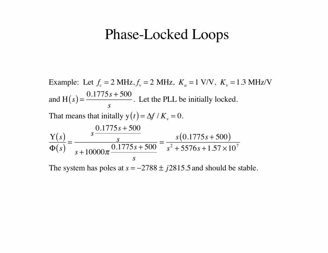
Example: Let fc = 2 MHz, fv = 2 MHz, Ka = 1 V/V, Kv = 1.3 MHz/V

and H s( ) = 0.1775s + 500s

. Let the PLL be initially locked.

That means that initally y t( ) = Δf / Kv = 0.

Y s( )Φ s( ) =

s 0.1775s + 500s

s +10000π 0.1775s + 500s

=s 0.1775s + 500( )

s2 + 5576s +1.57 ×107

The system has poles at s = −2788 ± j2815.5and should be stable.

Phase-Locked Loops

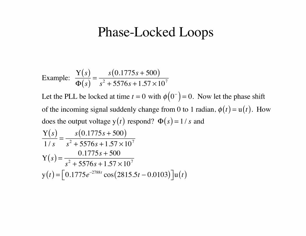
Example: Y s( )Φ s( ) =

s 0.1775s + 500( )s2 + 5576s +1.57 ×107

Let the PLL be locked at time t = 0 with φ 0−( ) = 0. Now let the phase shift

of the incoming signal suddenly change from 0 to 1 radian, φ t( ) = u t( ). Howdoes the output voltage y t( ) respond? Φ s( ) = 1 / s andY s( )1 / s

=s 0.1775s + 500( )

s2 + 5576s +1.57 ×107

Y s( ) = 0.1775s + 500s2 + 5576s +1.57 ×107

y t( ) = 0.1775e−2788t cos 2815.5t − 0.0103( )⎡⎣ ⎤⎦u t( )

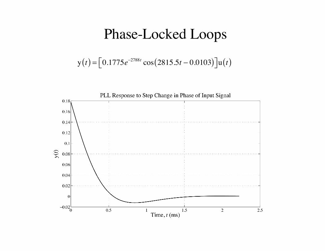
Phase-Locked Loops

y t( ) = 0.1775e−2788t cos 2815.5t − 0.0103( )⎡⎣ ⎤⎦u t( )

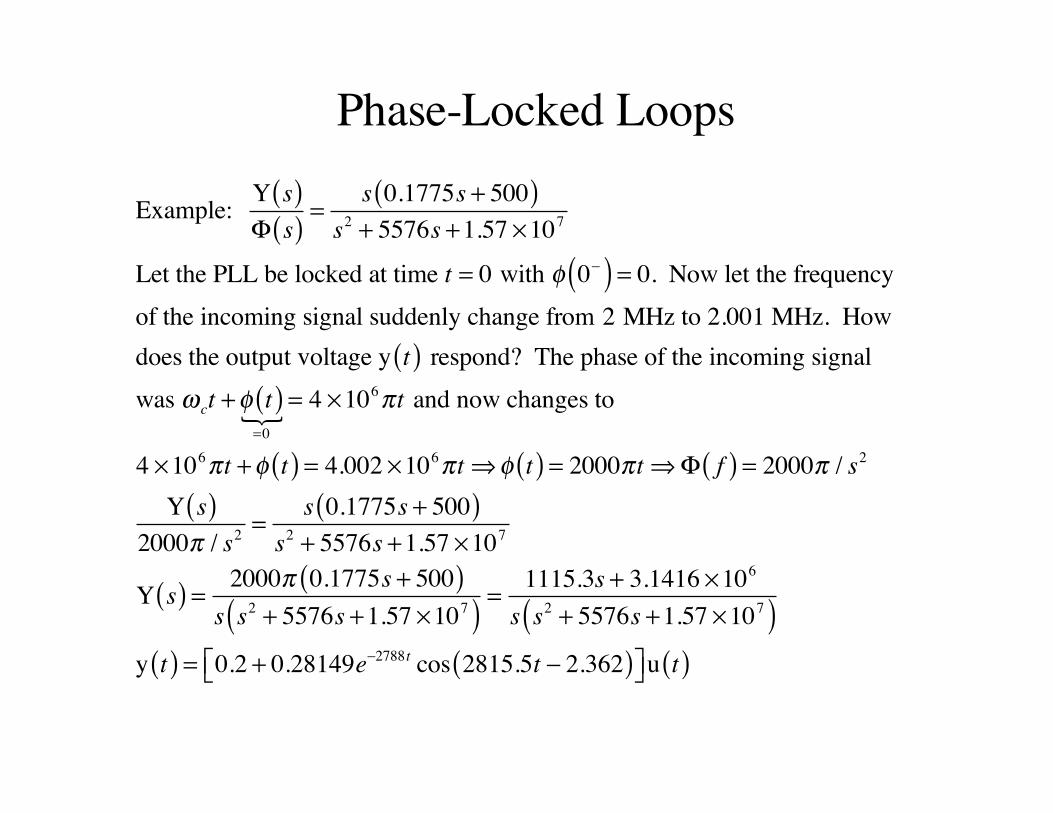
Phase-Locked Loops

Example: Y s( )Φ s( ) =

s 0.1775s + 500( )s2 + 5576s +1.57 ×107

Let the PLL be locked at time t = 0 with φ 0−( ) = 0. Now let the frequencyof the incoming signal suddenly change from 2 MHz to 2.001 MHz. Howdoes the output voltage y t( ) respond? The phase of the incoming signalwas ω ct +φ t( )

=0 = 4 ×106πt and now changes to

4 ×106πt +φ t( ) = 4.002 ×106πt⇒φ t( ) = 2000πt⇒Φ f( ) = 2000π / s2

Y s( )2000π / s2 =

s 0.1775s + 500( )s2 + 5576s +1.57 ×107

Y s( ) = 2000π 0.1775s + 500( )s s2 + 5576s +1.57 ×107( ) =

1115.3s + 3.1416 ×106

s s2 + 5576s +1.57 ×107( )y t( ) = 0.2 + 0.28149e−2788t cos 2815.5t − 2.362( )⎡⎣ ⎤⎦u t( )

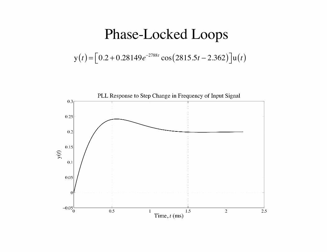
Phase-Locked Loopsy t( ) = 0.2 + 0.28149e−2788t cos 2815.5t − 2.362( )⎡⎣ ⎤⎦u t( )

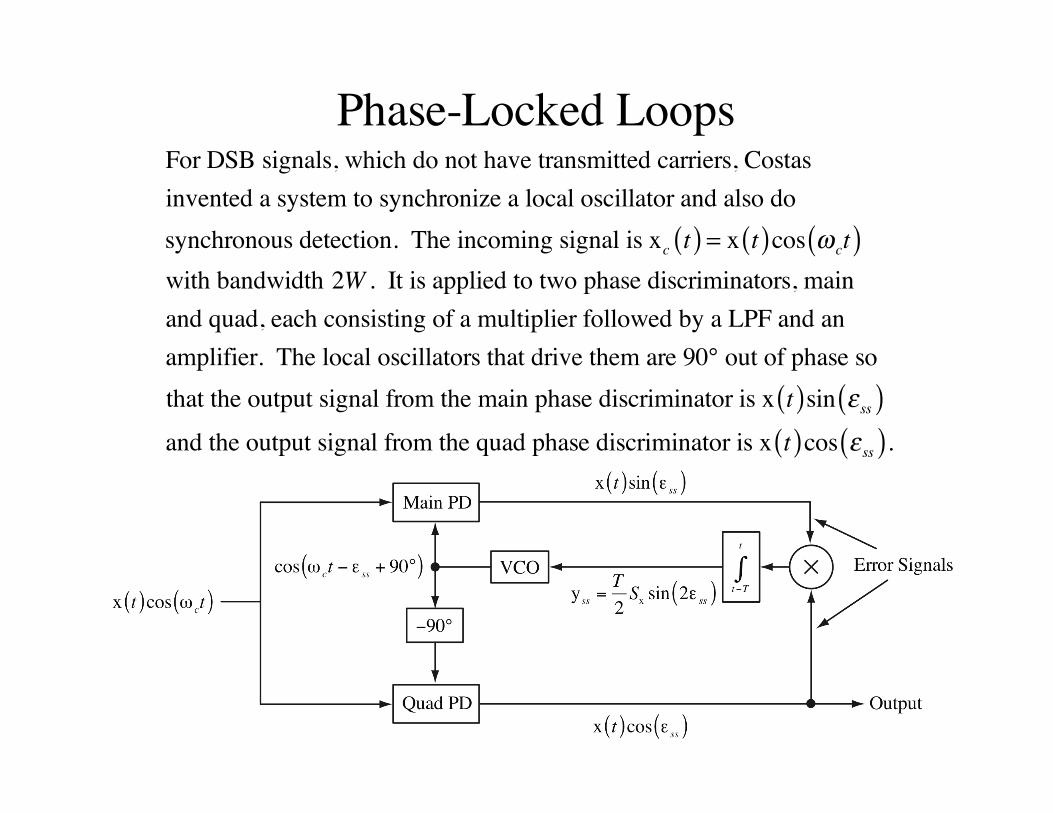
Phase-Locked LoopsFor DSB signals, which do not have transmitted carriers, Costasinvented a system to synchronize a local oscillator and also dosynchronous detection. The incoming signal is xc t( ) = x t( )cos ω ct( )with bandwidth 2W . It is applied to two phase discriminators, mainand quad, each consisting of a multiplier followed by a LPF and an amplifier. The local oscillators that drive them are 90° out of phase so that the output signal from the main phase discriminator is x t( )sin ε ss( )and the output signal from the quad phase discriminator is x t( )cos ε ss( ).

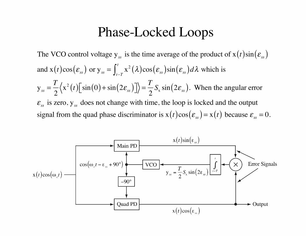
Phase-Locked LoopsThe VCO control voltage yss is the time average of the product of x t( )sin ε ss( )and x t( )cos ε ss( ) or yss = x2 λ( )cos ε ss( )sin ε ss( )dλ

t−T

t

∫ which is

yss =T2

x2 t( ) sin 0( ) + sin 2ε ss( )⎡⎣ ⎤⎦ = T2Sx sin 2ε ss( ). When the angular error

ε ss is zero, yss does not change with time, the loop is locked and the outputsignal from the quad phase discriminator is x t( )cos ε ss( ) = x t( ) because ε ss = 0.