transform signal and system - utkweb.eecs.utk.edu/~mjr/ece503/presentationslides/chapter...consider...

z Transform Signal and SystemAnalysis

5/10/04 M. J. Roberts - All Rights Reserved 2

Block Diagrams and TransferFunctions

Just as with CT systems, DT systems are convenientlydescribed by block diagrams and transfer functionscan be determined from them. For example, from thisDT system block diagram the difference equation canbe determined.

y x x yn n n n[ ] = [ ] − −[ ] − −[ ]2 112

1


Block Diagrams and TransferFunctions

From a z-domain block diagram the transfer function canbe determined.

Y X X Yz z z z z z( ) = ( )− ( )− ( )− −212

1 1

HYX

zzz

z

z

z

z( ) = ( )

( ) = −

+= −

+

−

−

2

112

2 112

1

1


Block Diagram Reduction

All the techniques for block diagram reduction introducedwith the Laplace transform apply exactly to z transformblock diagrams.


System Stability

A DT system is stable if its impulse responseis absolutely summable. That requirementtranslates into the z-domain requirement thatall the poles of the transfer function must liein the open interior of the unit circle.


System InterconnectionsCascade

Parallel


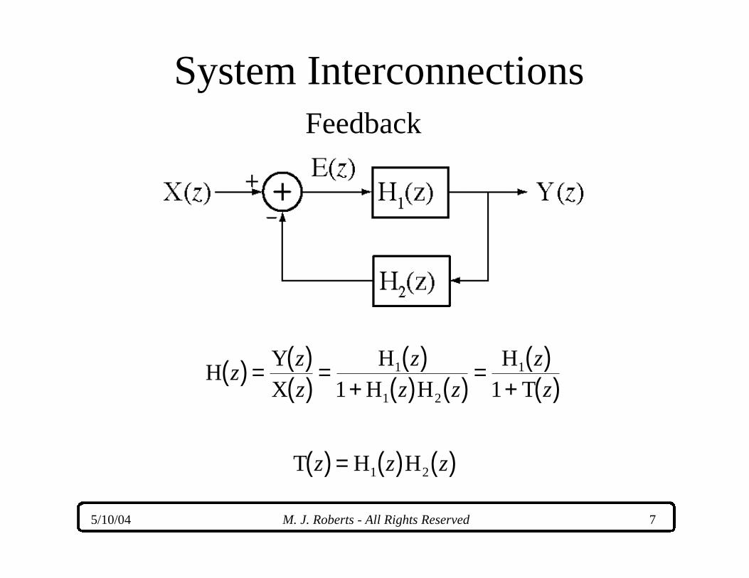
System Interconnections

HYX

HH H

HT

zzz

zz z

zz

( ) = ( )( ) = ( )

+ ( ) ( ) = ( )+ ( )

1

1 2

1

1 1

T H Hz z z( ) = ( ) ( )1 2

Feedback


Responses to Standard Signals

If the system transfer function is the z

transform of the unit-sequence response is

which can be written in partial-fraction form as

If the system is stable the transient term, , dies out

and the steady-state response is .

HND

zzz

( ) = ( )( )Y

ND

zz

zzz

( ) =−

( )( )1

YND

Hz zzz

zz

( ) = ( )( ) + ( )

−1 1

1

zzz

ND

1( )( )

H 11

( )−z

z


Responses to Standard Signals

Let the system transfer function be

Then

and

Let the constant, K be 1 - p. Then

H zKz

z p( ) =

−

Y zz

zKz

z pK

pz

zpz

z p( ) =

− −=

− −−

−

1 1 1

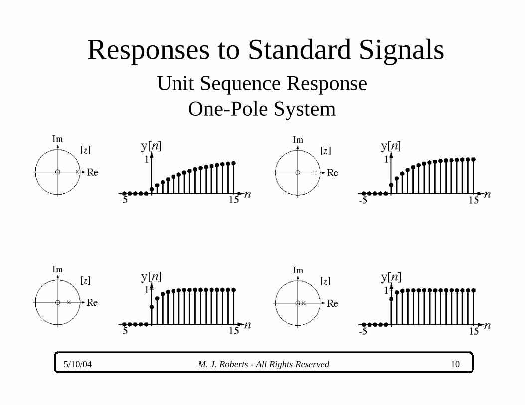
y unK

pp nn[ ] =

−−( ) [ ]+

11 1

y un p nn[ ] = −( ) [ ]+1 1


Responses to Standard SignalsUnit Sequence Response

One-Pole System


Responses to Standard SignalsUnit Sequence Response

Two-Pole System


Responses to Standard SignalsIf the system transfer function is the z transform

of the response to a suddenly-applied sinusoid is

Let . Then the system response can be written as

and, if the system is stable, the steady-state response is

a DT sinusoid with, generally, different magnitude and phase.

HND

zzz

( ) = ( )( )

YND

cos

cosz

zz

z z

z z( ) = ( )

( )− ( )[ ]

− ( ) +ΩΩ

02

02 1

y

N

DH cos Hn z

z

zp n p[ ] = ( )

( )

+ ( ) + ∠ ( )−Z 1 11 0 1Ω(( ) [ ]u n

H cos H up n p n1 0 1( ) + ∠ ( )( ) [ ]Ω

p e j1

0= Ω


For a stable system, the response to a suddenly-appliedsinusoid approaches the response to a true sinusoid (appliedfor all time).

Pole-Zero Diagrams andFrequency Response


Let the transfer function of a DT system be


H zz

zz

zz p z p

( ) =− +

=−( ) −( )2 1 2

25

16

pj

1

1 24

= +p

j2

1 24

= −

H ee

e p e pj

j

j jΩ

Ω

Ω Ω( ) =− −1 2


The Jury Stability Test

Let a transfer function be in the form,

where

Form the “Jury” array

HND

zzz

( ) = ( )( )

D z a z a z a z aDD

DD( ) = + + + +−

−1

11 0L

1

2

3

4

5

6

2 3

0 1 2 2 1

1 2 2 1 0

0 1 2 2 1

1 2 3 1 0

0 1 2 2

2 3 4 0

0 1 2

a a a a a a

a a a a a a

b b b b b

b b b b b

c c c c

c c c c

D s s s

D D D

D D D

D D

D D D

D

D D D

L

L

L

L

L

L

M M M M N

− −

− −

− −

− − −

−

− − −

−


The Jury Stability Test

The third row is computed from the first two by

The fourth row is the same set as the third row except inreverse order. Then the c’s are computed from the b’s inthe same way the b’s are computed from the a’s. This continues until only three entries appear. Then the system is stable if

ba a

a ab

a a

a ab

a a

a ab

a a

a aD

D

D

D

D

DD

D D0

0

01

0 1

12

0 2

21

0 1

1

= = = =− −−

−

, , , ,L

D 1 0( ) > −( ) −( ) >1 1 0D D

a a b b c c s sD D D> > > >− −0 0 1 0 2 0 2, , , ,L


Root LocusRoot locus methods for DT systems are like rootlocus methods for CT systems except that theinterpretation of the result is different.

CT systems: If the root locus crosses into theright half-plane the system goes unstable at thatgain.

DT systems: If the root locus goes outside theunit circle the system goes unstable at that gain.


Simulating CT Systems with DTSystems

The ideal simulation of a CT system by a DT system would havethe DT system’s excitation and response be samples from the CTsystem’s excitation and response. But that design goal is neverachieved exactly in real systems at finite sampling rates.



One approach to simulation is to make the impulse response ofthe DT system be a sampled version of the impulse response ofthe CT system.

With this choice, the response of the DT system to a DT unitimpulse consists of samples of the response of the CT system to aCT unit impulse. This technique is called impulse-invariantdesign.

h hn nTs[ ] = ( )



When the impulse response of the DT system is asampled version of the impulse response of the CT system but theunit DT impulse is not a sampled version of the unit CT impulse.

A CT impulse cannot be sampled. First, as a practical matterthe probability of taking a sample at exactly the time ofoccurrence of the impulse is zero. Second, even if the impulsewere sampled at its time of occurrence what would the samplevalue be? The functional value of the impulse is not defined at itstime of occurrence because the impulse is not an ordinaryfunction.

h hn nTs[ ] = ( )



In impulse-invariant design, even though the impulse response is asampled version of the CT system’s impulse response that does notmean that the response to samples from any arbitrary excitationwill be a sampled version of the CT system’s response to thatexcitation.

All design methods for simulating CT systems with DT systemsare approximations and whether or not the approximation is a goodone depends on the design goals.


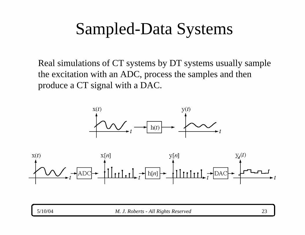
Sampled-Data Systems

Real simulations of CT systems by DT systems usually samplethe excitation with an ADC, process the samples and thenproduce a CT signal with a DAC.


Sampled-Data SystemsAn ADC simply samples a signal and produces numbers. Acommon way of modeling the action of a DAC is to imaginethe DT impulses in the DT signal which drive the DAC areinstead CT impulses of the same strength and that the DAChas the impulse response of a zero-order hold.



The desired equivalence between a CT and a DT system isillustrated below.

The design goal is to make look as much like aspossible by choosing h[n] appropriately.

yd t( ) yc t( )


Sampled-Data SystemsConsider the response of the CT system not to the actual signal,x(t), but rather to an impulse-sampled version of it,

The response is

where and the response at the nth multiple ofis

The response of a DT system with to the excitation, is

x x x combδ δt nT t nT t f f ts sn

s s( ) = ( ) −( ) = ( ) ( )=−∞

∞

∑

y h x h x x ht t t t m t mT m t mTsm

sm

( ) = ( )∗ ( ) = ( )∗ [ ] −( ) = [ ] −( )=−∞

∞

=−∞

∞

∑ ∑δ δ

x xn nTs[ ] = ( ) Ts

y x hnT m n m Ts sm

( ) = [ ] −( )( )=−∞

∞

∑h hn nTs[ ] = ( )

x xn nTs[ ] = ( )y x h x hn n n m n m

m

[ ] = [ ] ∗ [ ] = [ ] −[ ]=−∞

∞

∑



The two responses are equivalent in the sense that the values atcorresponding DT and CT times are the same.


Sampled-Data SystemsModify the CT system to reflect the last analysis.

Then multiply the impulse responses of both systems by Ts


Sampled-Data SystemsIn the modified CT system,

In the modified DT system,

where and h(t) still represents the impulseresponse of the original CT system. Now let approach zero.

This is the response, , of the original CT system.

y x h x h x ht t T t nT t nT t T nT t nT Ts s sn

s s s sn

( ) = ( )∗ ( ) = ( ) −( )

∗ ( ) = ( ) −( )

=−∞

∞

=−∞

∞

∑ ∑δ δ

y x h x hn m n m m T n m Tm

s sm

[ ] = [ ] −[ ] = [ ] −( )( )=−∞

∞

=−∞

∞

∑ ∑

h hn T nTs s[ ] = ( )Ts

lim y lim x h x hT T

s s sns s

t nT t nT T t d→ →

=−∞

∞

−∞

∞

( ) = ( ) −( ) = ( ) −( )∑ ∫0 0τ τ τ

yc t( )



Summarizing, if the impulse response of the DT system ischosen to be then, in the limit as the sampling rateapproaches infinity, the response of the DT system is exactlythe same as the response of the CT system.

Of course the sampling rate can never be infinite in practice.Therefore this design is an approximation which gets better asthe sampling rate is increased.

T nTs sh( )


Digital Filters

• Digital filter design is simply DT systemdesign applied to filtering signals

• A popular method of digital filter design is tosimulate a proven CT filter design

• There many design approaches each of whichyields a better approximation to the ideal asthe sampling rate is increased


Digital Filters

• Practical CT filters have infinite-durationimpulse responses, impulse responses whichnever actually go to zero and stay there

• Some digital filter designs produce DT filterswith infinite-duration impulse responses andthese are called IIR filters

• Some digital filter designs produce DT filterswith finite-duration impulse responses andthese are called FIR filters


Digital Filters

• Some digital filter design methods use time-domain approximation techniques

• Some digital filter design methods usefrequency-domain approximation techniques


Digital FiltersImpulse and Step Invariant Design


H s s( )

Impulse invariant:

h t( ) L−1 Sampleh n[ ] Z

H z z( )

Step invariant:

H s s( )×1

s H s ss( ) L−1

h− ( )1 tSample

h− [ ]1 n

Z zz

zz−( )

1H

× −zz

1

H z z( )

Impulse and Step Invariant DesignDigital Filters


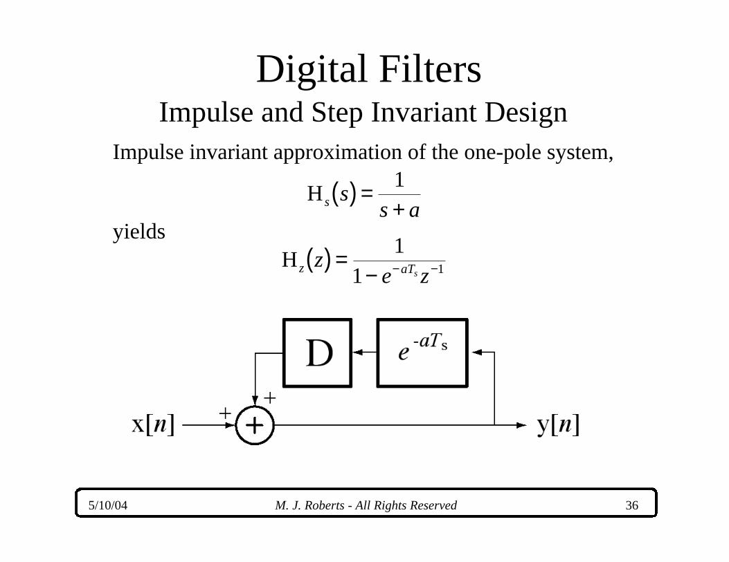
Impulse invariant approximation of the one-pole system,

yields

H s ss a

( ) =+1

H z aTze zs

( ) =− − −

11 1



Let a be one and let in H z aTze zs

( ) =− − −

11 1Ts = 0 1.

Digital FilterImpulse Response

CT FilterImpulse Response



Step response of H z aTze zs

( ) =− − −

11 1

Digital FilterStep Response

CT FilterStep Response

Notice scale difference



Digital FiltersWhy is the impulse response exactlyright while the step response is wrong?

This design method forces an equalitybetween the impulse strength of a CTexcitation, a unit CT impulse at zero,and the impulse strength of thecorresponding DT signal, a unit DTimpulse at zero. It also makes theimpulse response of the DT system,h[n], be samples from the impulseresponse of the CT system, h(t).


A CT step excitation is not an impulse. So what should thecorrespondence between the CT and DT excitations be now? If thestep excitation is sampled at the same rate as the impulse responsewas sampled, the resulting DT signal is the excitation of the DTsystem and the response of the DT system is the sum of theresponses to all those DT impulses.

Digital Filters


Digital FiltersIf the excitation of the CT system were a sequence of CT unitimpulses, occurring at the same sampling rate used to form h[n],then the response of the DT system would be samples of theresponse of theCT system.


Impulse invariant approximation of

with a 1 kHz sampling rate yields

H s ss

s s( ) =

+ + ×2 5400 2 10

H.

. .z

z zz z

( ) = −( )− +

0 91351 508 0 67032



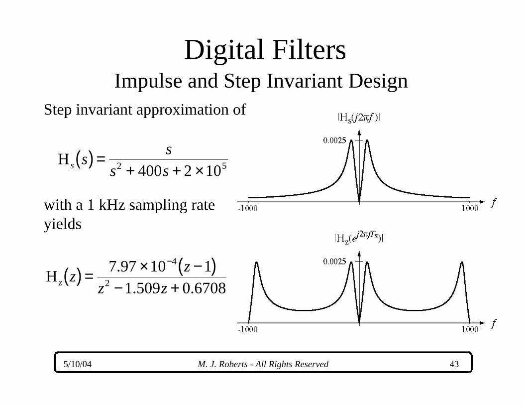
Step invariant approximation of

with a 1 kHz sampling rateyields

H s ss

s s( ) =

+ + ×2 5400 2 10

H.

. .z zz

z z( ) = × −( )

− +

−7 97 10 11 509 0 6708

4

2



Every CT transfer function implies a corresponding differentialequation. For example,

Derivatives can be approximated by finite differences.

H y y xs ss a

ddt

t a t t( ) =+

⇒ ( )( ) + ( ) = ( )1

ddt

tn n

Ts

yy y( )( ) ≅ +[ ] − [ ]1 d

dtt

n nTs

yy y( )( ) ≅ [ ] − −[ ]1

ddt

tn n

Ts

yy y( )( ) ≅ +[ ] − −[ ]1 1

2

Forward Backward

Central

Finite Difference DesignDigital Filters


Using a forward difference to approximate the derivative,

A more systematic method is to realize that every s in a CTtransfer function corresponds to a differentiation in the timedomain which can be approximated by a finite difference.

Hy y

y xss

ss a

n nT

a n n( ) =+

⇒ +[ ] − [ ] + [ ] = [ ]1 1

sz

Ts

→ −1s

z

Ts

→ − −1 1

sz z

Ts

→ − −1

2

Forward Backward Central

Digital FiltersFinite Difference Design


Then

H Hs zs

z

T

s

s

ss a

zs a

Tz aT

s

( ) =+

⇒ ( ) =+

=− −( )→ −

1 111



Finite difference approximation of


H s ss

s s( ) =

+ + ×2 5400 2 10

H.

. .z

z zz z

( ) = × −( )− +

−6 25 10 11 5 0 625

4

2



Direct substitution and matched filter design use the relationship, to map the poles and zeros of an s-domain transferfunction into corresponding poles and zeros of a z-domaintransfer function. If there is an s-domain pole or zero at a, the z-domain pole or zero will be at .

Direct Substitution

Matched z-Transform

Direct Substitution and Matched z-Transform Design

z esTs=

z esTs=

eaTs

s a z eaTs− → −

s a e zaTs− → − −1 1

Digital Filters


Matched z-transform approximation of


H s ss

s s( ) =

+ + ×2 5400 2 10

H. .z zz z

z z( ) = −( )

− +1

1 509 0 67082

Digital FiltersDirect Substitution and Matched z-Transform Design


This method is based on trying to match the frequency responseof a digital filter to that of the CT filter. As a practical matter itis impossible to match exactly because a digital filter has aperiodic frequency response, but a good approximation can bemade over a range of frequencies which can include all theexpected signal power.

The basic idea is to use the transformation,

to convert from the s to z domain.

sT

zs

→ ( )1ln e zsTs →or

Bilinear TransformationDigital Filters


The straightforward application of the transformation,would be the substitution,

But that yields a z-domain function that is a transcendentalfunction of z with infinitely many poles. The exponentialfunction can be expressed as the infinite series,

and then approximated by truncating the series.

sT

zs

→ ( )1ln

H Hlnz s s

Tz

z ss

( ) = ( ) → ( )1

e xx x x

kx

k

k

= + + + + ==

∞

∑12 3

2 3

0! ! !L

Digital FiltersBilinear Transformation


Truncating the exponential series at two terms yields thetransformation,

or

This approximation is identical to the finite difference methodusing forward differences to approximate derivatives. Thismethod has a problem. It is possible to transform a stable s-domain function into an unstable z-domain function.

+ →sT zs

szTs

→ −1



The stability problem can be solved by a very clevermodification of the idea of truncating the series. Express theexponential as

Then approximate both numerator and denominator with atruncated series.

This is called the bilinear transformation because both numeratorand denominator are linear functions of z.

ee

e

zsT

sT

sT

s

s

s= →

−

2

2

12

12

+

−→

sT

sTz

s

s

sT

zzs

→ −+

2 11



The bilinear transformationhas the quality that everypoint in the s plane maps intoa unique point in the z plane,and vice versa. Also, the lefthalf of the s plane maps intothe interior of the unit circlein the z plane so a stable s-domain system istransformed into a stable z-domain system.



The bilinear transformation is unique among the digital filter designmethods because of the unique mapping of points between the twocomplex planes. There is however a “warping” effect. It can be seenby mapping real frequencies in the z plane (the unit circle) intocorresponding points in the s plane (the ω axis). Letting with

Ω real, the corresponding contour in the s plane is

or

z e j= Ω

sT

ee

jTs

j

js

= −+

=

2 11

22

Ω

ΩΩ

tan

Ω =

−22

1tanωTs



Bilinear approximation of


H s ss

s s( ) =

+ + ×2 5400 2 10

H. .

zz

z z( ) = −

− +

2

2

11 52 0 68



FIR digital filters are based on theidea of approximating an idealimpulse response. Practical CTfilters have infinite-duration impulseresponses. The FIR filterapproximates this impulse bysampling it and then truncating it toa finite time (N impulses in theillustration).

FIR FiltersDigital Filters


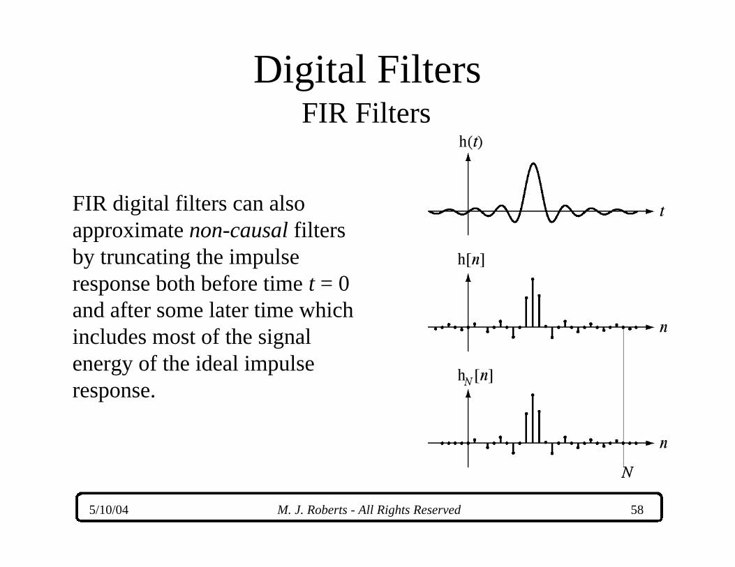
FIR digital filters can alsoapproximate non-causal filtersby truncating the impulseresponse both before time t = 0and after some later time whichincludes most of the signalenergy of the ideal impulseresponse.

Digital FiltersFIR Filters


The design of an FIRfilter is the essence ofsimplicity. It consists ofmultiple feedforwardpaths, each with adifferent delay andweighting factor and allof which are summed toform the response.

hN mm

N

n a n m[ ] = −[ ]=

−

∑ δ0

1



Since this filter has no feedback paths its transfer function is of theform,

and it is guaranteed stable because it has N - 1 poles, all of whichare located at z = 0.

HN mm

m

N

z a z( ) = −

=

−

∑0

1



The effect of truncating an impulse response can be modeled bymultiplying the ideal impulse response by a “window” function. Ifa CT filter’s impulse response is truncated between t = 0 and t = T,the truncated impulse response is

where, in this case,

hh ,

,h wT t

t t Tt t( ) =

( ) < <

= ( ) ( )0

0 otherwise

w recttt

T

T( ) =

−

2



The frequency-domain effect of truncating an impulse response isto convolve the ideal frequency response with the transform of thewindow function.

If the window is a rectangle,

H HT f f W f( ) = ( )∗ ( )

W sincf T Tf e j fT( ) = ( ) − π



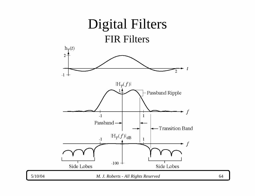
Let the ideal transfer function beThe corresponding impulse response is

The truncated impulse response is

The transfer function for the truncated impulse response is

H rectffB

e j fT( ) =

−

2π

h sinc rectT t B B tT t

T

T( ) = −

−

2 22

2

h sinct B B tT( ) = −

2 2

2

H rect sincTj fT j fTf

fB

e T Tf e( ) =

∗ ( )− −

2π π



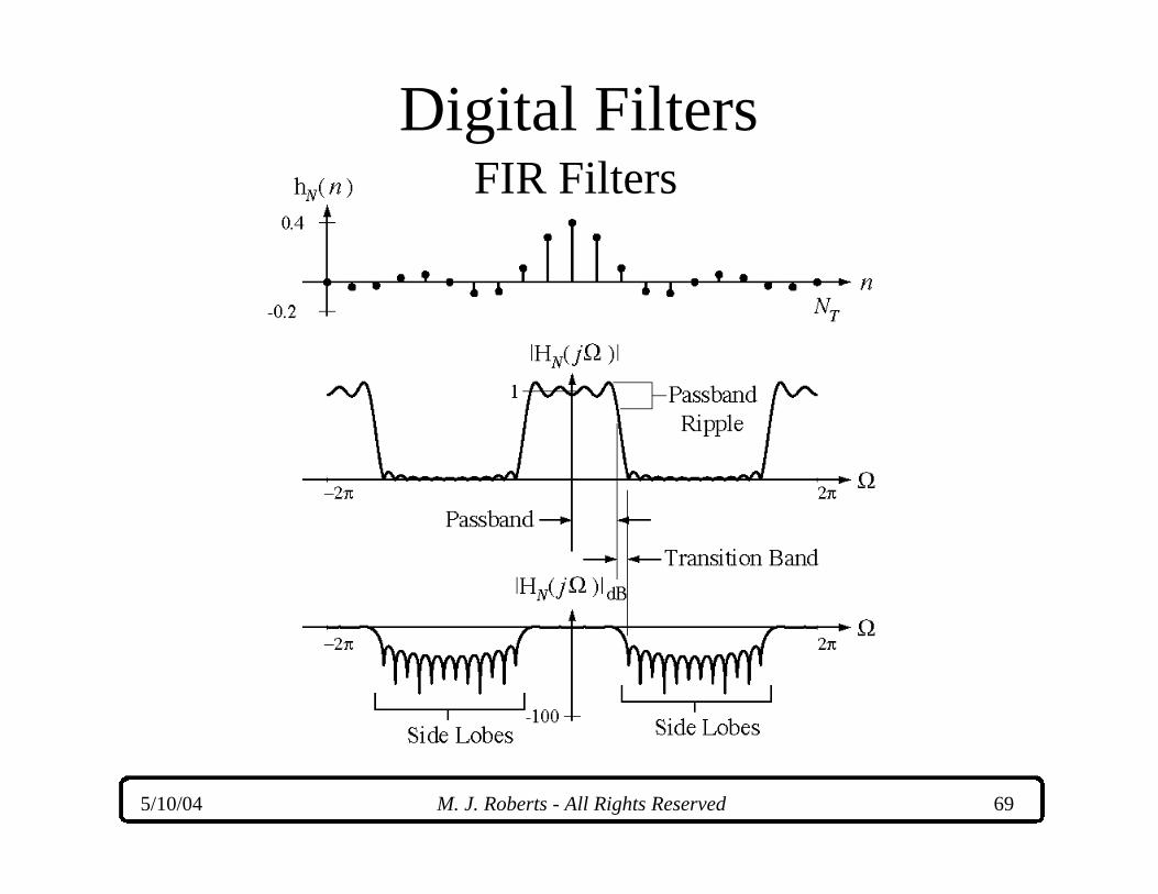
The effects of windowing a digital filter’s impulse response aresimilar to the windowing effects on a CT filter.

hh ,

,h wN n

n n Nn n[ ] =

[ ] ≤ <

= [ ] [ ]0

0 otherwise

H H WN j j jΩ Ω Ω( ) = ( ) ( )



The “ripple” effect in the frequency domain can be reduced byusing windows of different shapes. The shapes are chosen tohave DTFT’s which are more confined to a narrow range offrequencies. Some commonly-used windows are

1. von Hann

2. Bartlett

w cos ,nn

Nn N[ ] = −

−

≤ <12

12

10

π

w,

,n

nN

nN

nN

Nn N

[ ] = −≤ ≤ −

−−

− ≤ <

21

01

2

22

11

2



3. Hamming

4. Blackman

5. Kaiser

w . . cos ,nn

Nn N[ ] = −

−

≤ <0 54 0 46

21

0π

w . . cos . cos ,nn

Nn

Nn N[ ] = −

−

+

−

≤ <0 42 0 5

21

0 084

10

π π

w n

IN

nN

IN

a

a

[ ] =

−

− − −

−

0

2 2

0

12

12

12

ω

ω

(windows continued)



Windows Window Transforms



Standard Realizations

• Realization of a DT system closely parallelsthe realization of a CT system

• The basic forms, canonical, cascade andparallel have the same structure

• A CT system can be realized with integrators,summers and multipliers

• A DT system can be realized with delays,summers and multipliers



Canonical

Delay

Summer

Multiplier



Cascade


Standard RealizationsParallel


State-Space AnalysisIn DT system state-space analysis the “next” state-variable valuesare set equal to a linear combination of the “present” state-variablevalues and the “present” excitations. The system and outputequations are

For this system,q Aq Bx y Cq Dxn n n n n n+[ ] = [ ] + [ ] [ ] = [ ] + [ ]1 ,

q nn

n[ ] =

[ ][ ]

q

q1

2

A =

13

14

12

0

B =

1 0

0 1x n

n

n[ ] =

[ ][ ]

x

x1

2

y n n[ ] = [ ][ ]y C = [ ]2 3

D = [ ]0 0


State-Space AnalysisFor illustration purposed let the excitation vector be

and let the system be initiallyat rest. Then by directrecursion,

x nn

n[ ] =

[ ][ ]

u

δ

n n n nq q y

. . .

. . .

1 2

0 0 0 0

1 1 1 5

2 1 5833 0 5 4 667

3 1 6528 0 7917 5 681

[ ] [ ] [ ]

M M M M


State-Space AnalysisThe recursion process proceeds as follows

and

q Aq Bx

q Aq Bx A q ABx Bx

q Aq Bx A q A Bx ABx Bx

q A q A Bx A Bx

1 0 0

2 1 1 0 0 1

3 2 2 0 0 1 2

0 0 1

2

3 2

1 2

[ ] = [ ] + [ ][ ] = [ ] + [ ] = [ ] + [ ] + [ ][ ] = [ ] + [ ] = [ ] + [ ] + [ ] + [ ]

[ ] = [ ] + [ ] + [ ] + +− −

M

Ln n n n AA Bx A Bx1 02 1n n−[ ] + −[ ]

y Cq Dx CAq CBx Dx

y Cq Dx CA q CABx CBx Dx

y Cq Dx CA q CA Bx CABx CBx Dx

y CA

1 1 1 0 0 1

2 2 2 0 0 1 2

3 3 3 0 0 1 2 3

2

3 2

[ ] = [ ] + [ ] = [ ] + [ ] + [ ][ ] = [ ] + [ ] = [ ] + [ ] + [ ] + [ ][ ] = [ ] + [ ] = [ ] + [ ] + [ ] + [ ] + [ ]

[ ] =

M

n nqq CA Bx CA Bx CA Bx Dx0 0 1 11 2 0[ ] + [ ] + [ ] + + −[ ] + [ ]− −n n n nL


State-Space AnalysisThe recursions can be written in the more compact forms,

These two equations can be written in the forms,

where (pp. 866-867).

y CA q C A Bx Dxn m nn n m

m

n

[ ] = [ ] + [ ] + [ ]− −

=

−

∑0 1

0

1

q A q A Bxn mn n m

m

n

[ ] = [ ] + [ ]− −

=

−

∑0 1

0

1

Zero-Input Response Zero-State

Response

q q Bxn n n n n[ ] = [ ] [ ] + −[ ] −[ ] ∗ [ ]− −

φ φ0 1 1zero excitation

responsezero stateresponse

124 34 1 2444 3444u

y C q C Bx Dxn n n n n n[ ] = [ ] [ ] + −[ ] −[ ] ∗ [ ] + [ ]φ φ0 1 1u

An n= [ ]φ


State-Space AnalysisAn alternate to the previous discrete-time-domain solution ofthe state and output equations is to solve them using the ztransform. Transforming the system equation,

by comparing this equation with a previous one,

it is apparent that and therefore

z z z z zQ q AQ BX( )− [ ] = ( )+ ( )0

Q I A BX q I A BX I A qz z z z z z z z( ) = −[ ] ( )+ [ ][ ] = −[ ] ( )+ −[ ] [ ]− −

−

−

−

1 1 10 0zero stateresponse

zero excitationresponse

1 244 344 1 244 344

φ n z z[ ]← → −[ ]−Z I A 1

q q Bxn n n n n[ ] = [ ] [ ] + −[ ] −[ ] ∗ [ ]− −

φ φ0 1 1zero excitation

responsezero stateresponse

124 34 1 2444 3444u

Φ z z z( ) = −[ ]−I A 1


State-Space AnalysisLet the excitation vector again be and let the systembe initially at rest.

Inverse transforming (pg. 868),

x nn

n[ ] =

[ ][ ]

u

δ

Q zz

z

zz( ) =

− −

−

−

−13

14

12

1 0

0 1 11

1

Q z z z z

z z z

( ) = −−

−−

+

−−

−+

+

1 8461

0 5780 5575

0 2680 2242

0 9231

0 5190 5575

0 5960 2242

. ..

..

. ..

..

q n nn n

n n[ ] =− ( ) − −( )− ( ) + −( )

−[ ]

−( ) −( )

−( ) −( )1 846 0 578 0 5575 0 268 0 2242

0 923 0 519 0 5575 0 596 0 22421

1 1

1 1

. . . . .

. . . . .u


State-Space AnalysisThe response vector is easily found from the state-variablevector.

The closed-form solution has the same initial values as the recursion solution indicating it is probably correct.

y n nn n[ ] = − ( ) + −( )[ ] −[ ]−( ) −( )6 461 2 713 0 5575 1 252 0 2242 11 1. . . . . u

n n n nq q y

. . .

. . .

1 2

0 0 0 0

1 1 1 5

2 1 5833 0 5 4 667

3 1 6528 0 7917 5 681

[ ] [ ] [ ]

M M M M


State-Space Analysis

Some other results of state-space analysis that are similar tothose from the CT-system case are

If and then

where and and

where and .

H C I A B Dz z( ) = −[ ] +−1

q Tq2 1n n[ ] = [ ] q A q B x1 1 1 11n n n+[ ] = [ ] + [ ]q A q B x2 2 2 21n n n+[ ] = [ ] + [ ]

A TA T2 11= − B TB2 1=

y C q D xn n n[ ] = [ ] + [ ]2 2 2

C C T2 11= − D D2 1=

Transfer Function

transform signal and system - utkweb.eecs.utk.edu/~mjr/ece503/presentationslides/chapter...consider...

Documents