analysis and design of metamaterial-inspired microwave ... · microwave structures and antenna...
TRANSCRIPT

Loughborough UniversityInstitutional Repository
Analysis and design ofmetamaterial-inspired
microwave structures andantenna applications
This item was submitted to Loughborough University's Institutional Repositoryby the/an author.
Additional Information:
• A Doctoral Thesis. Submitted in partial fulfillment of the requirementsfor the award of Doctor of Philosophy of Loughborough University.
Metadata Record: https://dspace.lboro.ac.uk/2134/6094
Publisher: c© Titos Kokkinos
Please cite the published version.

This item was submitted to Loughborough’s Institutional Repository (https://dspace.lboro.ac.uk/) by the author and is made available under the
following Creative Commons Licence conditions.
For the full text of this licence, please go to: http://creativecommons.org/licenses/by-nc-nd/2.5/
Analysis and Design of Metamaterial-Inspired Microwave
Structures and Antenna Applications
by
Titos Kokkinos
A doctoral thesis submitted in conformity with the requirementsfor the degree of Doctorate of Philosophy
Department of Electronic and Electrical EngineeringLoughborough University
Copyright c© 2010 by Titos Kokkinos

Abstract
Analysis and Design of Metamaterial-Inspired Microwave Structures and Antenna
Applications
Titos Kokkinos
Doctorate of Philosophy
Department of Electronic and Electrical Engineering
Loughborough University
2010
Novel metamaterial and metamaterial-inspired structures and microwave/antenna ap-
plications thereof are proposed and studied in this thesis. Motivated by the challenge
of extending the applicability of metamaterial structures into practical microwave so-
lutions, the underlying objective of this thesis has been the design of low-cost, easily
fabricated and deployable metamaterial-related devices, and the development of com-
putational tools for the analysis of those. For this purpose, metamaterials composed
of tightly coupled resonators are chosen for the synthesis of artificial transmission lines
and enabling antenna applications. Specifically, fully-printed double spiral resonators
are employed as modular elements for the design of tightly coupled resonators arrays.
After thoroughly investigating the properties of such resonators, they are used for the
synthesis of artificial lines in either grounded or non-grounded configurations. In the
first case, the supported backward waves are exploited for the design of microstrip-based
filtering/diplexing devices and series-fed antenna arrays. In the second case, the effective
properties of such structures are employed for the design of a novel class of self-resonant,
low-profile folded monopoles, exhibiting low mutual coupling and robust radiating prop-
erties. Such monopoles are, in turn, used for the synthesis of different sub-wavelength
antenna arrays, such as superdirective arrays. Finally, an in-house periodic FDTD-based
computational tool is developed and optimized for the efficient and rigorous analysis of
planar, metamaterial-based, high-gain antennas.
ii

To my wife, Eirini.
iii

Acknowledgements
Although doctorate research tends to be a quite lonely process, it becomes much
more fruitful, efficient and enjoyable through the interaction with people that share the
same research interests. During my doctorate studies in Loughborough University I had
the chance to collaborate with researchers and academics that possess solid technical
backgrounds and high research qualities. Now, that this endeavor reaches its end, I feel
the moral obligation to thank all of them by heart and wish them all the best in their
personal and professional lives.
First of all, I gratefully thank my supervisor Dr Alexandros P. Feresidis for his
guidance, patience, understanding and encouragement during this research endeavor.
Throughout my doctoral studies Alex has been extremely supportive and always avail-
able to help towards overcoming the encountered technical difficulties and suggest new
research directions.
Together with Alex, I would also like to thank all the faculty members of the WiCR
and CMCR groups, namely Prof. Yiannis Vardaxoglou, Dr Rob Edwards, Dr James Flint
and Rob Seager, and the post-doctoral researchers Dr James Kelly, Dr Alford Chauraya,
Dr Panagiotis Kosmas and Dr George Goussetis, for all the interaction we had during
the last four years.
I would like also to thank the technicians of the Department of Electronic and Elec-
trical Engineering Terry West, Peter Godfrey and Peter Harrison, whose help with the
fabrication of some of the prototypes has been invaluable.
Special thanks go to the fellow graduate students of WiCR Stratos Doumanis, George
Palikaras, Marta Padilla-Pardo and Nikos Christopoulos, the MSc students Eirini Liakou,
Tomas Rufete and Anestis Katsounaros that I had the chance to work with, and all the
other members of WiCR and CMCR.
Given that part of the writing up of this thesis was carried out while being with
Bell Laboratories Ireland, Alcatel-Lucent, I would also like to thank my colleagues Dr
Andrei Grebennikov and Dr Florian Pivit for all the stimulating discussions during the
last ten months, and my manager Dr Francis Mullany for providing me the working hours
flexibility required for the conclusion of the writing up and the submission of the thesis.
Also, I would like to acknowledge the financial support, through a scholarship for
graduate studies and multiple travel grants, of EPSRC, the Department of Electronic
and Electrical Engineering, the Faculty of Engineering, Loughborough University, and
iv

the European Antennas Virtual Center of Excellence.
Last but definitely not least, I would like to express my deepest gratitude to my life
partner and wife Eirini, who, throughout these years, has been consistently supportive,
patient and willing to undergo several personal sacrifices in order for this research en-
deavor to be concluded. Eirini, thank you for being at my side, thank you for being
yourself.
v

Publications from the Research
Aspects of the work of this thesis have been published or accepted for publication in
the following papers.
Referred Journal Papers
• T. Kokkinos, and A. P. Feresidis,“Low-Profile Folded Monopoles with Embedded
Planar Metamaterial Phase-Shifting Lines”, IEEE Transactions on Antennas and
Propagation, to appear, Oct. 2009.
• T. Kokkinos, E. Liakou and A. P. Feresidis,“Decoupling antenna elements of PIFA
arrays on handheld devices”, Electronics Letters, vol. 44, no. 25, pp. 1442-1444,
Dec. 2008.
• J. R. Kelly, T. Kokkinos, and A. P. Feresidis,“Analysis and Design of Subwave-
length Resonant Cavity Type 2-D Leaky-Wave Antennas”, IEEE Transactions on
Antennas and Propagation, vol. 56, no. 9, pp. 2817-2825, Sept. 2008.
Referred Conference Papers
• A.P. Feresidis, T. Kokkinos and Q. Li, “Isolation Enhancement of Monopole An-
tennas and PIFAs on a Compact Ground Planes”, to be presented in Proc. IEEE
LAPC 2009, Loughborough, UK.
• T. Kokkinos and A.P. Feresidis, “An Electrically Small Monopole-Like Antenna
with Embedded Metamaterial High-µ Matching Network”, Proc. Metamaterials
2008, Pamplona, Spain, Sept. 2008 (oral presenantion) (Best Student Paper Award
Finalist).
• T. Kokkinos, T. Rufete-Martinez and A.P. Feresidis, “lectrically Small Superdirec-
tive Endfire Arrays of Low-Profile Folded Monopoles”, Proc. Metamaterials 2008,
Pamplona, Spain, Sept. 2008 (oral presentation).
• T. Kokkinos, A. Katsounaros and A.P. Feresidis, “Series-Fed Microstrip Patch Ar-
rays Employing Metamaterial Transmission Lines: A Comparative Study” Proc.
IET EuCAP 2007, Edinburgh UK, Nov. 2007 (poster presentation).
vi

• T. Kokkinos, A.P. Feresidis and J.C. Vardaxoglou, “A Low-profile Monopolelike
Small Antenna with Embedded Metamaterial Spiral-based Matching Network”,
Proc. IET EuCAP 2007, Edinburgh UK, Nov. 2007 (poster presentation).
• J. R. Kelly, T. Kokkinos, and A. P. Feresidis, “Modeling and Design of a Subwave-
length Resonant Cavity Antenna” Proc. Metamaterials 2007, Rome, Oct. 2007
(oral presentation).
• T. Kokkinos, A.P. Feresidis and J.C. Vardaxoglou, “Equivalent Circuit of Double
Spiral Resonators Supporting Backward Waves”, Proc. IEEE LAPC 2007, Lough-
borough, UK (poster presentation).
• T. Kokkinos, A.P. Feresidis and J.C. Vardaxoglou, “Analysis and Application of
Metamaterial Spiral-Based Transmission Lines” Proc. IWAT 2007, Cambridge, UK
(oral presentation).
• T. Kokkinos, A.P. Feresidis and J.C. Vardaxoglou, “On the Use of Spiral Res-
onators for the Design of Uniplanar Microstrip-Based Left-Handed Metamaterials”,
Proc. 2006 IEEE European Conference on Antennas and Propagation, Nice, France
(poster presentation).
Other aspects of the work of this thesis have been recently submitted for publication
or remain under submission.
vii

Contents
1 Introduction 1
1.1 Electromagnetic Metamaterials . . . . . . . . . . . . . . . . . . . . . . . 1
1.2 Metamaterial and Metamaterial-Inspired Applications . . . . . . . . . . . 6
1.3 Motivation . . . . . . . . . . . . . . . . . . . . . . . . . . . . . . . . . . . 8
1.4 Aim and Overview of the Thesis . . . . . . . . . . . . . . . . . . . . . . . 9
2 Theoretical Background 12
2.1 Synthesis and Analysis of Metamaterial Structures Considering Arbitrary
Resonators and Their Equivalent Circuits . . . . . . . . . . . . . . . . . . 12
2.1.1 General . . . . . . . . . . . . . . . . . . . . . . . . . . . . . . . . 12
2.1.2 Free-Standing Resonators Interacting with Plane Waves . . . . . . 13
Resonators Magnetically Coupled to Plane Waves . . . . . . . . . 13
Resonators Electrically Coupled to Plane Waves . . . . . . . . . . 17
Examples of Resonators . . . . . . . . . . . . . . . . . . . . . . . 20
Metamaterial Applications . . . . . . . . . . . . . . . . . . . . . . 21
2.1.3 Arrays of Tightly Coupled Resonators . . . . . . . . . . . . . . . 22
Electrically Coupled Resonators . . . . . . . . . . . . . . . . . . . 24
Magnetically Coupled Resonators . . . . . . . . . . . . . . . . . . 26
Metamaterial Applications . . . . . . . . . . . . . . . . . . . . . . 29
2.1.4 Discussion . . . . . . . . . . . . . . . . . . . . . . . . . . . . . . . 30
2.2 Periodic FDTD Analysis of Metamaterial Structures . . . . . . . . . . . . 30
2.2.1 The Finite-Difference Time-Domain Technique . . . . . . . . . . . 31
Maxwell’s Equations in the FDTD Technique . . . . . . . . . . . 31
2.2.2 Floquet’s Theorem . . . . . . . . . . . . . . . . . . . . . . . . . . 35
Floquet’s Theorem in Frequency-Domain . . . . . . . . . . . . . . 35
Floquet’s Theorem in Time-Domain . . . . . . . . . . . . . . . . . 36
viii

2.2.3 Periodic Boundary Conditions in the FDTD Technique . . . . . . 37
General . . . . . . . . . . . . . . . . . . . . . . . . . . . . . . . . 37
Sine-Cosine Method . . . . . . . . . . . . . . . . . . . . . . . . . 37
Sine-Cosine Method in Practice . . . . . . . . . . . . . . . . . . . 39
2.2.4 Applications of the Periodic FDTD-based Tool . . . . . . . . . . . 43
Dispersion Analysis of Periodic Structures . . . . . . . . . . . . . 43
Modal Field Patterns Extraction . . . . . . . . . . . . . . . . . . 44
Analysis of Leaky-Wave Structures . . . . . . . . . . . . . . . . . 44
2.3 Commercial Electromagnetic Solvers . . . . . . . . . . . . . . . . . . . . 44
2.3.1 General . . . . . . . . . . . . . . . . . . . . . . . . . . . . . . . . 44
2.3.2 Ansoft HFSS . . . . . . . . . . . . . . . . . . . . . . . . . . . . . 45
2.3.3 Ansoft Designer . . . . . . . . . . . . . . . . . . . . . . . . . . . . 45
2.3.4 CST Microwave Studio . . . . . . . . . . . . . . . . . . . . . . . . 45
3 Spiral-based Artificial Transmission Lines and Applications 47
3.1 Review of Artificial Transmission Lines . . . . . . . . . . . . . . . . . . . 47
3.2 Double Spiral Resonators . . . . . . . . . . . . . . . . . . . . . . . . . . . 48
3.2.1 Description . . . . . . . . . . . . . . . . . . . . . . . . . . . . . . 48
3.2.2 Periodic Analysis . . . . . . . . . . . . . . . . . . . . . . . . . . . 50
Dispersion Analysis . . . . . . . . . . . . . . . . . . . . . . . . . . 50
Modal Field Patterns . . . . . . . . . . . . . . . . . . . . . . . . . 51
3.2.3 Equivalent Circuit . . . . . . . . . . . . . . . . . . . . . . . . . . 53
Lossless Approach . . . . . . . . . . . . . . . . . . . . . . . . . . 54
Impact of Losses . . . . . . . . . . . . . . . . . . . . . . . . . . . 56
3.3 Analysis of Coupled DSR . . . . . . . . . . . . . . . . . . . . . . . . . . . 58
3.3.1 DSR Coupling Configurations . . . . . . . . . . . . . . . . . . . . 58
3.3.2 DSR Coupling Assessment . . . . . . . . . . . . . . . . . . . . . . 62
3.4 1-D DSR-based Artificial Transmission Lines . . . . . . . . . . . . . . . . 65
3.4.1 Simulation . . . . . . . . . . . . . . . . . . . . . . . . . . . . . . . 65
3.4.2 Fabrication and Measurements . . . . . . . . . . . . . . . . . . . . 66
3.4.3 Impact of Losses . . . . . . . . . . . . . . . . . . . . . . . . . . . 69
3.5 DSR-based Artificial Transmission Lines Applications . . . . . . . . . . . 71
3.5.1 Series-Fed Patch Arrays . . . . . . . . . . . . . . . . . . . . . . . 71
General . . . . . . . . . . . . . . . . . . . . . . . . . . . . . . . . 71
ix

Proposed study . . . . . . . . . . . . . . . . . . . . . . . . . . . . 72
Fabrication and Measurements . . . . . . . . . . . . . . . . . . . . 74
4 A Metamaterial Low-Profile Monopole-Like Antenna 81
4.1 Introduction . . . . . . . . . . . . . . . . . . . . . . . . . . . . . . . . . . 81
4.2 Proposed Antenna Design - General Description . . . . . . . . . . . . . . 85
4.3 Spiral-Based Phase-Shifting Lines . . . . . . . . . . . . . . . . . . . . . . 87
4.4 Equivalent Circuit . . . . . . . . . . . . . . . . . . . . . . . . . . . . . . 90
4.5 Low-Profile Antenna at 2.4 GHz . . . . . . . . . . . . . . . . . . . . . . . 92
4.5.1 Antenna Parameters and Full-wave Simulations . . . . . . . . . . 92
4.5.2 Fabrication and Measurement . . . . . . . . . . . . . . . . . . . . 96
4.5.3 Q-factor calculation . . . . . . . . . . . . . . . . . . . . . . . . . . 99
4.6 Towards Ultra Low-Profile Folded Monopoles . . . . . . . . . . . . . . . 100
4.7 Impact of the Ground Plane . . . . . . . . . . . . . . . . . . . . . . . . . 103
4.7.1 Reducing the Ground Plane Size . . . . . . . . . . . . . . . . . . 103
4.7.2 Antenna Designs on a λ/2 × λ/2 Ground Plane . . . . . . . . . . 105
λ/9 folded-monopole on a λ/2 × λ/2 ground plane . . . . . . . . . 105
λ/17 folded-monopole on a λ/2 × λ/2 ground plane . . . . . . . . 106
4.8 Microstrip-fed Low-Profile Folded Monopoles . . . . . . . . . . . . . . . . 109
4.9 Coupling Assessment Between Low-Profile Folded Monopoles . . . . . . . 112
4.9.1 Full-wave Analysis . . . . . . . . . . . . . . . . . . . . . . . . . . 113
Inter-element spacing : 0.2λ . . . . . . . . . . . . . . . . . . . . . 113
Inter-element spacing : 0.15λ . . . . . . . . . . . . . . . . . . . . 113
4.9.2 Analytical Approach . . . . . . . . . . . . . . . . . . . . . . . . . 114
5 Sub-wavelength Antenna Arrays 117
5.1 Introduction . . . . . . . . . . . . . . . . . . . . . . . . . . . . . . . . . . 117
5.2 Sub-wavelength Phased Arrays . . . . . . . . . . . . . . . . . . . . . . . 119
5.3 Sub-wavelength Superdirective Endfire Arrays . . . . . . . . . . . . . . . 123
5.3.1 General . . . . . . . . . . . . . . . . . . . . . . . . . . . . . . . . 123
5.3.2 Feeding Network . . . . . . . . . . . . . . . . . . . . . . . . . . . 124
5.3.3 Driven Superdirective Arrays . . . . . . . . . . . . . . . . . . . . 126
0.2λ Array . . . . . . . . . . . . . . . . . . . . . . . . . . . . . . . 127
0.15λ Array . . . . . . . . . . . . . . . . . . . . . . . . . . . . . . 128
x

5.3.4 0.1λ Parasitic Array . . . . . . . . . . . . . . . . . . . . . . . . . 130
5.3.5 Comparison . . . . . . . . . . . . . . . . . . . . . . . . . . . . . . 131
5.4 Decoupling PIFAs on Handhelds . . . . . . . . . . . . . . . . . . . . . . . 133
6 Periodic FDTD Analysis of Leaky-Wave Antennas 141
6.1 Introduction . . . . . . . . . . . . . . . . . . . . . . . . . . . . . . . . . . 141
6.2 Periodic FDTD Analysis of LWA . . . . . . . . . . . . . . . . . . . . . . 142
6.2.1 Background . . . . . . . . . . . . . . . . . . . . . . . . . . . . . . 142
6.2.2 An Improved Methodology . . . . . . . . . . . . . . . . . . . . . . 145
6.2.3 Validation of the Improved Methodology . . . . . . . . . . . . . . 146
Metal-strip-loaded dielectric rod LWA . . . . . . . . . . . . . . . . 146
Partially-reflective-surface (PRS) half-wavelength LWA . . . . . . 148
6.2.4 Large alpha Values Assessment . . . . . . . . . . . . . . . . . . . 149
6.3 Periodic FDTD Analysis of Sub-wavelength Resonant Cavity Type 2-D
LWA . . . . . . . . . . . . . . . . . . . . . . . . . . . . . . . . . . . . . . 152
6.4 Radiation Pattern Calculation of Finite-size LWAs Using Periodic FDTD
Simulations . . . . . . . . . . . . . . . . . . . . . . . . . . . . . . . . . . 157
6.4.1 General . . . . . . . . . . . . . . . . . . . . . . . . . . . . . . . . 157
6.4.2 Electromagnetic Behavior of Finite-size LWA . . . . . . . . . . . . 158
6.4.3 Array Factor of Finite-size LWA . . . . . . . . . . . . . . . . . . . 160
Proposed Model . . . . . . . . . . . . . . . . . . . . . . . . . . . . 160
Validation - Discussion . . . . . . . . . . . . . . . . . . . . . . . . 163
7 Conclusions 167
7.1 Review . . . . . . . . . . . . . . . . . . . . . . . . . . . . . . . . . . . . . 167
7.2 Future Work . . . . . . . . . . . . . . . . . . . . . . . . . . . . . . . . . . 169
A Analysis Of Coupled Lines 172
xi

List of Tables
2.1 Location of field components on the Yee’s space lattice (according to the
convention of this thesis). . . . . . . . . . . . . . . . . . . . . . . . . . . 33
2.2 Points on the Yee’s cell at which the partial spatial derivatives of the field
components are calculated (according to the convention of this thesis). . 34
2.3 Methods that have been proposed for the application of periodic boundary
conditions in time-domain [1]. . . . . . . . . . . . . . . . . . . . . . . . 37
2.4 Pairs of field elements arrays of the computational domain of Fig. 2.19
that are involved in the application of the periodic boundary conditions. 41
4.1 Resonance and fractional bandwidth of the four antennas of different profiles.102
4.2 Input resistance, radiation resistance and simulated radiating efficiency
(at resonance) of the four antennas of different profiles. . . . . . . . . . . 102
4.3 Coupling coefficients between pairs of λ/4 monopoles and the proposed
low-profile folded monopoles (LPFM) for different inter-element distances. 114
5.1 Comparative study of the three antenna designs with enhanced directivities.133
6.1 Cavity heights and MGP parameters of the investigated antenna structures.154
xii

List of Figures
2.1 Schematic representation of an LC resonator inductively coupled to an
impinging plane wave. . . . . . . . . . . . . . . . . . . . . . . . . . . . . 14
2.2 a) Lumped-element circuit model for a plane wave magnetically coupled
to a free-standing LC resonator. b) Equivalent circuit of the model a). . 15
2.3 Relative effective constitutive parameters when free-space is loaded with
inductively excited resonators. The parameters of the resonators are Lo =
3.0 nH, Co = 1.0 pF , fo = 2.906 GHz, kM = 0.5 and d = 3 mm . . . . . . 16
2.4 Dispersion analysis of the unit cell of Fig. 2.2(b) extracted through the
periodic analysis of [2]. . . . . . . . . . . . . . . . . . . . . . . . . . . . . 18
2.5 Schematic representation of an LC resonator electrically coupled to an
impinging plane wave. . . . . . . . . . . . . . . . . . . . . . . . . . . . . 18
2.6 a) Lumped-element circuit model for a plane wave electrically coupled to
a free-standing LC resonator. b) Equivalent circuit of the model a). . . . 19
2.7 Relative effective constitutive parameters when free-space is loaded with
capacitively excited resonators. The parameters of the resonators are Lo =
3.0 nH, Co = 1.0 pF , fo = 2.906 GHz, kE = 0.5 and d = 3 mm . . . . . . 20
2.8 The well-known split-ring resonator [3] has been extensively used in the
literature for the synthesis of artificial magnetodielectrics. . . . . . . . . . 21
2.9 The well-known dipole resonator. Arrays of such resonators can be used
for the synthesis of artificial dielectrics. . . . . . . . . . . . . . . . . . . . 22
2.10 Equivalent circuit of a medium loaded with both magnetically and elec-
trically excited resonators. By properly tuning the two resonators, left-
handed modes may be supported by the loaded medium. . . . . . . . . . 23
2.11 An array of tightly coupled resonators. In the general case, the resonators
may be both electrically (kE) and magnetically (kM) coupled. . . . . . . 24
xiii

2.12 A unit cell of the array of Fig. 2.11, where the resonators are considered
to be exclusively electrically coupled. . . . . . . . . . . . . . . . . . . . . 24
2.13 Equivalent circuit of the unit cell of Fig. 2.12. The coupling mechanism
has been represented with an admittance inverter J = ωCm . . . . . . . . 25
2.14 Dispersion relation (2.26) for different values of the coupling coefficient |kE|. 26
2.15 L − C resonators array consisted of magnetically coupled resonators. . . 27
2.16 Equivalent circuit of the structural unit cell of the magnetically coupled
resonators array. In this unit cell the inductive coupling mechanism is
represented with an equivalent impedance inverter K = ωLm. . . . . . . 27
2.17 Dispersion relation (2.34) for different values of the coupling coefficient |kM |. 29
2.18 Yee’s cell. . . . . . . . . . . . . . . . . . . . . . . . . . . . . . . . . . . . 33
2.19 Computational domain used for the FDTD analysis of a two-dimensional
periodic structure (only TM modes are assumed). . . . . . . . . . . . . . 40
2.20 Flow chart of the algorithm that is used for the application of periodic
boundary conditions, through the sine-cosine method, in the FDTD tech-
nique. . . . . . . . . . . . . . . . . . . . . . . . . . . . . . . . . . . . . . 42
2.21 Square unit cell (dashed line) and its reciprocal irreducible Brillouin zone
(solid line). . . . . . . . . . . . . . . . . . . . . . . . . . . . . . . . . . . 43
3.1 Schematic of a double spiral resonator. In our approach, the spiral is to
be printed on a grounded substrate. The figure should be also assumed to
be the computational domain of the full-wave periodic analysis. . . . . . 49
3.2 a) Open-loop resonator. b) Double spiral can be formed by wounding the
open ends of the open-loop resonator. . . . . . . . . . . . . . . . . . . . . 49
3.3 Dispersion diagram of the unit cell of Fig. 3.1. The first formulated
passband (fundamental mode) is clearly a backward wave band. . . . . . 51
3.4 Modal field pattern of the electric field component oriented along x−axis
for the mode that is supported at fo = 3.4 GHz and propagating along
x−axis (kxdx = π/2,kydy = 0). . . . . . . . . . . . . . . . . . . . . . . . . 52
3.5 Modal field pattern of the electric field component oriented along z−axis
for the mode that is supported at fo = 3.4 GHz and propagating along
x−axis (kxdx = π/2,kydy = 0). . . . . . . . . . . . . . . . . . . . . . . . . 53
xiv
3.6 Modal field pattern of the magnetic field component oriented along z−axis
for the mode that is supported at fo = 3.4 GHz and propagating along
x−axis (kxdx = π/2,kydy = 0). . . . . . . . . . . . . . . . . . . . . . . . . 54
3.7 Equivalent circuit of the DSR of Fig. 3.1 (lossless case). . . . . . . . . . 55
3.8 Equivalent circuit of the DSR of Fig. 3.1 (including losses). . . . . . . . . 56
3.9 Normalized transmission through a weakly excited DSR calculated using
the equivalent circuit of Fig. 3.8 and Ansoft Designer. . . . . . . . . . . 57
3.10 Four possible scenarios and equivalent lumped-element representation for
two inductively coupled spirals, depending on their polarities (windings of
the spirals) and the sign of the coupling coefficient (direction of the flowing
currents and the corresponding magnetic flux). . . . . . . . . . . . . . . 60
3.11 Exact equivalent circuits of the four scenarios of Fig. 3.10. For all the
equivalent circuits, regardless of the sign of kM , Lm = kMLo . . . . . . . 61
3.12 Ansoft Designer model used for the calculation of the transmission through
a weakly excited pair of coupled DSRs. In this configuration, the double
spirals have been arranged symmetrically along the axis of propagation
(as in Fig. 3.10(a) ). . . . . . . . . . . . . . . . . . . . . . . . . . . . . . 63
3.13 Ansoft Designer model used for the calculation of the transmission through
a weakly excited pair of coupled DSRs. In this configuration, the double
spirals have been arranged asymmetrically along the axis of propagation
(each spiral is rotated by 180o compared to its adjacent spirals) (as in Fig.
3.10(e) ). . . . . . . . . . . . . . . . . . . . . . . . . . . . . . . . . . . . . 63
3.14 Simulated transmission through the weakly excited pair of coupled DSR
of Fig. 3.12. . . . . . . . . . . . . . . . . . . . . . . . . . . . . . . . . . . 64
3.15 Simulated transmission through the weakly excited pair of coupled DSRs
of Fig. 3.13. . . . . . . . . . . . . . . . . . . . . . . . . . . . . . . . . . . 64
3.16 Top view of a DSR-based transmission line composed of 4 DSR and em-
bedded within a common 50 Ω microstrip line. . . . . . . . . . . . . . . . 66
3.17 Simulated S−parameters of the transmission line of Fig. 3.16. . . . . . . 67
3.18 Fabricated prototype of a spiral-based transmission line that is composed
of six unit cells. . . . . . . . . . . . . . . . . . . . . . . . . . . . . . . . 67
3.19 Measured and simulated S11 of the prototype of Fig. 3.18. . . . . . . . . 68
3.20 Measured and simulated S21of the prototype of Fig. 3.18. . . . . . . . . . 68
xv

3.21 Measured unwrapped transmission phases of two DSR-based transmission
lines that are composed of 4 and 6 unit cells, respectively. . . . . . . . . 69
3.22 Simulated power losses across a 4-unit-cell spiral-based transmission line
for several cases of ohmic and dielectric losses. . . . . . . . . . . . . . . . 70
3.23 Measured power losses across a 4-unit-cell and a 6-unit-cell spiral-based
transmission line. . . . . . . . . . . . . . . . . . . . . . . . . . . . . . . . 71
3.24 Analytically calculated directivity of a three-element and a four-element
microstrip patch array, as a function of the distance between any pair of
neighboring patches. . . . . . . . . . . . . . . . . . . . . . . . . . . . . . 73
3.25 Array factors of a three-element (point A in Fig. 3.24) and a four-element
array (point B in Fig. 3.24) occupying the same area. . . . . . . . . . . 74
3.26 a) Three-element series-fed array, incorporating conventional interconnect-
ing lines, that corresponds to point A of Fig. 3.24 and b) four-element
series-fed array, incorporating artificial DSR-based interconnecting lines,
that corresponds to point B of Fig. 3.24. . . . . . . . . . . . . . . . . . . 75
3.27 Photograph of the fabricated three- and four-element series-fed array pro-
totypes. . . . . . . . . . . . . . . . . . . . . . . . . . . . . . . . . . . . . 77
3.28 Measured return loss of the conventional three-element array. . . . . . . . 77
3.29 Measured return loss of the four-element array. . . . . . . . . . . . . . . . 78
3.30 Measured E-plane radiation patterns of the three-element and four-element
patch arrays at 2.4 GHz. . . . . . . . . . . . . . . . . . . . . . . . . . . . 79
3.31 E-plane radiation patterns of the four-element array at frequencies 2.31GHz,
2.40 GHz and 2.49 GHz. . . . . . . . . . . . . . . . . . . . . . . . . . . . 80
4.1 Schematic representation of a) the typical folded monopole of height h1 =
λ/4 and b) a low-profile folded monopole with an embedded metamaterial
phase-shifting line. . . . . . . . . . . . . . . . . . . . . . . . . . . . . . . 82
4.2 a) Side view and b) top view schematic of the proposed low-profile antenna. 86
4.3 Unit cell of a) a free standing DSR and b) a DSR participating in an array. 87
4.4 Equivalent circuit representation of the unit cells of a) Fig. 4.3(a) and b)
Fig. 4.3(b). . . . . . . . . . . . . . . . . . . . . . . . . . . . . . . . . . . 88
4.5 Coupling scenarios for a pair of spirals and equivalent circuit representa-
tions. Lss corresponds to the self-inductance of each of the spirals and
Lm = |kM |Lss to the absolute value of their mutual inductance. . . . . . 89
xvi

4.6 Dispersion curves of the unit cell of Fig. 4.4(b) for positive and negative
values of the coupling coefficient kM . . . . . . . . . . . . . . . . . . . . . 89
4.7 Transmission magnitude and phase through a single unit cell similar with
that of Fig. 4.4(b) for a positive coupling coefficient (kM > 0). . . . . . . 90
4.8 Equivalent circuit of the proposed low-profile folded monopole antenna. . 90
4.9 Input resistance of the antenna of section 4.2 calculated using the equiva-
lent circuit of Fig. 4.8 and Ansoft HFSS simulations. . . . . . . . . . . . 93
4.10 Input reactance of the antenna of section 4.2 calculated using the equiva-
lent circuit of Fig. 4.8 and Ansoft HFSS simulations. . . . . . . . . . . . 93
4.11 Simulated input impedance of the proposed antenna. . . . . . . . . . . . 95
4.12 Currents on the vertical posts at 2.36 GHz. . . . . . . . . . . . . . . . . 95
4.13 Simulated (using Ansoft HFSS) transmission magnitude and phase when
both posts are terminated with coaxial ports (none of the ports is shorted
in this case). . . . . . . . . . . . . . . . . . . . . . . . . . . . . . . . . . . 96
4.14 Measured and simulated return loss of the proposed antenna. . . . . . . . 97
4.15 Measured (Wheeler cap method) and simulated (Ansoft HFSS) radiation
efficiency of the proposed antenna. . . . . . . . . . . . . . . . . . . . . . 98
4.16 Simulated E−plane (xz−plane) of the proposed low-profile folded monopole,
built on a 2λ × 2λ ground plane. . . . . . . . . . . . . . . . . . . . . . . 99
4.17 Simulated H−plane (xy−plane) of the proposed low-profile folded monopole,
built on a 2λ × 2λ ground plane. . . . . . . . . . . . . . . . . . . . . . . 99
4.18 Simulated input resistance of four antennas of different profiles. . . . . . 101
4.19 Simulated input reactance of four antennas of different profiles. . . . . . . 101
4.20 Simulated reflection coefficient of four antennas of different profiles. . . . 102
4.21 Simulated radiation efficiency of four antennas of different profiles. The
dots on the traces denote the resonance of each antenna design. . . . . . 103
4.22 Simulated input reactance of the λ/9 folded monopole built on ground
planes of different sizes. . . . . . . . . . . . . . . . . . . . . . . . . . . . . 104
4.23 Simulated input reflection coefficient of the λ/9 folded monopole built on
ground planes of different sizes. . . . . . . . . . . . . . . . . . . . . . . . 104
4.24 Photograph of the proposed λ/9 folded monopole built on a λ/2 × λ/2
ground plane. . . . . . . . . . . . . . . . . . . . . . . . . . . . . . . . . . 105
4.25 Measured and simulated return loss of the λ/9 folded monopole built on
a λ/2 × λ/2 ground plane. . . . . . . . . . . . . . . . . . . . . . . . . . . 106
xvii

4.26 Measured and simulated E−plane radiation pattern of the λ/9 folded
monopole built on a λ/2 × λ/2 ground plane. . . . . . . . . . . . . . . . 107
4.27 Measured and simulated H−plane radiation pattern of the λ/9 folded
monopole built on a λ/2 × λ/2 ground plane. . . . . . . . . . . . . . . . 107
4.28 a) Top view and b) side view photograph of the λ/17 low-profile folded
monopole built on a λ/2 × λ/2 ground plane. . . . . . . . . . . . . . . . 108
4.29 Measured and simulated return loss of the λ/17 folded monopole built on
a λ/2 × λ/2 ground plane. . . . . . . . . . . . . . . . . . . . . . . . . . . 108
4.30 Measured and simulated E−plane radiation pattern of the λ/17 folded
monopole built on a λ/2 × λ/2 ground plane. . . . . . . . . . . . . . . . 109
4.31 Measured and simulated H−plane radiation pattern of the λ/17 folded
monopole built on a λ/2 × λ/2 ground plane. . . . . . . . . . . . . . . . 109
4.32 a) Top view and b) side view schematic of the microstrip-fed low-profile
antenna. . . . . . . . . . . . . . . . . . . . . . . . . . . . . . . . . . . . . 110
4.33 a) Side view and b)top view photograph of the microstrip-fed low-profile
antenna. . . . . . . . . . . . . . . . . . . . . . . . . . . . . . . . . . . . . 110
4.34 Simulated and measured return loss of the microstip-fed single element. . 111
4.35 E-plane radiation pattern for a single low-profile folded monopole fed with
a microstrip line. . . . . . . . . . . . . . . . . . . . . . . . . . . . . . . . 112
4.36 H-plane radiation pattern for a single low-profile folded monopole fed with
a microstrip line. . . . . . . . . . . . . . . . . . . . . . . . . . . . . . . . 112
4.37 Return loss and coupling coefficient between two λ/4 monopoles and two
low-profile folded monopoles (LPFM), respectively, being 0.2λ apart. . . 113
4.38 Return loss and coupling coefficient between two λ/4 monopoles and two
low-profile folded monopoles (LPFM), respectively, being 0.15λ apart. . . 114
4.39 Configurations for the calculation of the mutual inductances supported
between a pair of a) λ/4 monopoles and b) the proposed low-profile folded
monopoles. . . . . . . . . . . . . . . . . . . . . . . . . . . . . . . . . . . . 115
4.40 Mutual inductance supported between two λ/4 monopoles and two low-
profile folded monopoles as a function of the distance between them. . . . 116
5.1 Microstrip-based feeding network employed for the synthesis of the two-
element sub-wavelength phased array. . . . . . . . . . . . . . . . . . . . . 120
5.2 S−parameters (magnitude) of the feeding network of Fig. 5.1. . . . . . . 121
xviii

5.3 S−parameters (phase) of the feeding network of Fig. 5.1. . . . . . . . . . 121
5.4 Photograph of the fabricated prototype of the investigated sub-wavelength
phased array of low-profile folded monopoles. . . . . . . . . . . . . . . . . 122
5.5 Measured return losses (S11) of the two sub-wavelength arrays. . . . . . . 122
5.6 H−plane patterns of the two compared sub-wavelength arrays. . . . . . . 123
5.7 Relative excitation phase, according to the analysis of [4], for the design
of two-element superdirective arrays. . . . . . . . . . . . . . . . . . . . . 125
5.8 Top view schematic of the modified ring hybrid used as feeding network
for the proposed superdirective endfire two-element array designs. . . . . 125
5.9 Insertion loss and phase difference between the two output ports of the
modified hybrid of Fig. 5.8. . . . . . . . . . . . . . . . . . . . . . . . . . 126
5.10 A schematic representation of the proposed superdirective arrays. . . . . 127
5.11 Photograph of the fabricated two-element superdirective endfire array. . . 127
5.12 Return loss for the 0.2λ superdirective endfire array. . . . . . . . . . . . . 128
5.13 H−plane radiation pattern for the 0.2λ array prototype compared with
that of a single low-profile monopole. The orientation of the 2-element
array with respect to the measured pattern has been noted with the two
dots in the middle of the plot (each dot represents each element of the
array). . . . . . . . . . . . . . . . . . . . . . . . . . . . . . . . . . . . . . 129
5.14 Return loss for the 0.15λ superdirective enfdire array. . . . . . . . . . . . 130
5.15 H−plane radiation patterns for the 0.15λ array prototype and the single
monopole. The orientation of the 2-element array with respect to the
measured pattern has been noted with the two dots in the middle of the
plot (each dot represents each element of the array). . . . . . . . . . . . . 130
5.16 Return loss for the 0.1λ parasitic array. . . . . . . . . . . . . . . . . . . . 132
5.17 H−plane radiation patterns for the 0.10λ array prototype and the single
monopole. The orientation of the 2-element array with respect to the
measured pattern has been noted with the two dots in the middle of the
plot (each dot represents each element of the array). . . . . . . . . . . . . 132
5.18 Layout of the a) single PIFA element, b) two-element array on handheld
(no slits on the ground plane), c) coupling reduction scheme by inserting
a single slit (notch) on the ground plane, d) coupling reduction scheme by
inserting two coupled slits at a distance d from each other. . . . . . . . . 135
xix

5.19 Simulated (using CST MWS) S−parameters of the two-element array in
the cases that no slits (original design), one slit, two slits and two resonat-
ing coupled slits have been inserted on the common ground plane. . . . . 137
5.20 Ground plane currents and normal electric field for the resonating effective
magnetic loop. . . . . . . . . . . . . . . . . . . . . . . . . . . . . . . . . . 138
5.21 Radiation patterns comparison between the conventional and the decou-
pled PIFA arrays at 1.85 GHz. . . . . . . . . . . . . . . . . . . . . . . . 139
5.22 Measured S−parameters for the configurations of Fig. 5.18(b) and Fig.
5.18(d), when d = 11mm. Due to fabrication imperfections, the resonance
of the coupled slits is achieved at 1.92 GHz. . . . . . . . . . . . . . . . . 140
6.1 Time-domain waveform extracted from the simulation of a non-radiating
structure using the periodic FDTD technique presented in chapter 2. . . 143
6.2 Time-domain waveform extracted from the simulation of a leaky-wave
structure using the periodic FDTD technique presented in chapter 2. . . 143
6.3 Generic representation of the periodic FDTD computational domain re-
quired for the implementation of equation (6.3). . . . . . . . . . . . . . . 144
6.4 Unit cell of the metal-strip-loaded dielectric rod LWA, as modeled through
the periodic FDTD analysis. . . . . . . . . . . . . . . . . . . . . . . . . 147
6.5 Complex propagation constant calculation for the leaky-mode supported
by the antenna of Fig. 6.4 calculated using both equation (6.3) and the
improved methodology. . . . . . . . . . . . . . . . . . . . . . . . . . . . . 148
6.6 a) Schematic representation of the dipole-based partially-reflective-surface
(PRS) half-wavelength leaky-wave structure of [5]. b) Computational do-
main used for the periodic FDTD analysis of the unit cell of the structure
of a). . . . . . . . . . . . . . . . . . . . . . . . . . . . . . . . . . . . . . 149
6.7 Complex propagation constant values of the perturbed, x−axis propagat-
ing TE1 mode, calculated using the lossy medium approach [5] and the
proposed improved methodology. . . . . . . . . . . . . . . . . . . . . . . 150
6.8 Error in α calculation using the lossy medium approach the improved
methodology as a function of the magnitude of α. . . . . . . . . . . . . . 151
xx

6.9 Schematic representation of the investigated sub-wavelength resonant cav-
ity type 2-D leaky-wave antennas. a) Cross-section of the investigated an-
tennas, b)top-view of the employed PRS and c) top-view of the employed
MGP. . . . . . . . . . . . . . . . . . . . . . . . . . . . . . . . . . . . . . 153
6.10 Side view of the computational domain employed for the periodic FDTD
analysis of the sub-wavelength resonant cavity type 2-D LWAs. . . . . . 155
6.11 Phase constant of the supported TE leaky-modes. . . . . . . . . . . . . . 156
6.12 Attenuation constants of the leaky-modes shown in Fig. 6.11. . . . . . . 156
6.13 Normalized attenuation constant as a function of cavity height for three
different PRSs. . . . . . . . . . . . . . . . . . . . . . . . . . . . . . . . . 156
6.14 Top view of a finite size resonant cavity type 2-D LWA. If the structure
is excited with an x−axis oriented current source, a TE wave will be
supported along z−axis and a TM wave along x−axis. The TE wave will
correspond the yz−plane to the H-plane of the antenna and the TM wave
would create an E-plane in the xy-plane. . . . . . . . . . . . . . . . . . 158
6.15 Dispersion relations of the TE1 and TM1 modes supported by a λ/2 par-
allel plate waveguide with a cut-off frequency at 3.7 GHz . . . . . . . . . 160
6.16 Impedances of the TE1 and TM1 modes supported by a λ/2 parallel plate
waveguide with a cut-off frequency at 3.7 GHz. . . . . . . . . . . . . . . 160
6.17 Reflection coefficients for the TE and TM wave impinging at the open ends
of a finite size waveguide structure (with a cut-off frequency at 3.7 GHz),
when diffraction effects are not considered. . . . . . . . . . . . . . . . . . 161
6.18 Array representation of a cross section of a finite size LWA along any of
its principal planes. . . . . . . . . . . . . . . . . . . . . . . . . . . . . . . 161
6.19 E- and H-plane radiation patterns of a λ/4.9 resonant cavity type 2-D
leaky-wave antenna composed of 13 unit cells, calculated using the pro-
posed model. . . . . . . . . . . . . . . . . . . . . . . . . . . . . . . . . . 164
6.20 E- and H-plane radiation patterns of a λ/4.9 resonant cavity type 2-D
leaky-wave antenna composed of 13 unit cells, calculated using the a full-
wave simulation of the entire finite size structure (obtained from [6]). . . 164
A.1 Microstrip lines coupled under an even-mode excitation. In that case a
magnetic wall can be assumed between the lines and, therefore, no capac-
itance is supported between them. . . . . . . . . . . . . . . . . . . . . . . 173
xxi

A.2 Microstrip lines coupled under an odd-mode excitation. In that case an
electric wall can be assumed between the lines and, therefore, a fringing
field capacitance is supported between them. . . . . . . . . . . . . . . . . 173
xxii

Chapter 1
Introduction
This chapter offers a general introduction to the thesis. Initially, a brief but inclusive
introduction to electromagnetic metamaterials is attempted. In the second section of the
chapter, the major classes of metamaterial applications are described. The reasons that
motivated this research endeavor are discussed in the third section of the chapter, while
an overview of the thesis is offered in the last section of the chapter.
1.1 Electromagnetic Metamaterials
Electromagnetic metamaterials constitute an extended class of electromagnetic struc-
tures that has attracted significant interest among electromagnetic engineers, microwave
engineers and physicists during the last decade. Deriving its name from the Greek prefix
µǫτα−, meaning beyond, the term “metamaterial” had been originally employed to de-
scribe any artificial (engineered) structure possessing effective electromagnetic properties
not encountered among natural materials.
The first theoretical study of the properties of a hypothetical medium possessing un-
natural electromagnetic parameters was pursued in 1967 by V.G. Veselago who examined
the electromagnetic properties of an ideal medium that possesses simultaneously negative
values of its electric permittivity ǫ and its magnetic permeability µ [7]. In this study,
Veselago showed that when both ǫ and µ are negative, the phase constant β = ω√
ǫµ of a
wave that propagates in that medium remains real allowing the electromagnetic waves to
propagate without any attenuation, losses or internal reflections. By means of Maxwell’s
equations, he proved that in such a medium the electric field E, the magnetic field H and
the wave vector k form a left-handed triplet, in contrast to the ordinary media where they
1

Chapter 1. Introduction 2
form a right-handed triplet. Therefore, media with simultaneously negative values of ǫ
and µ are nowadays called Left-Handed Media (LHM). Also, by comparing the direction
of the wave vector k to the Pointing vector S, defined as S = E×H∗ and always forming
a right-handed triplet with the electric and magnetic field components, he concluded that
in media that simultaneously exhibit negative ǫ and µ the wave vector k and the Poynting
vector S are contra-directional, as opposed to common right-handed media where they
are co-directed. This suggests that in LHM the power flows in the opposite direction
of phase progression or, equivalently, that the group velocity ug and the phase velocity
uϕ are antiparallel. The electromagnetic waves which are characterized by antiparallel
group and phase velocities are called backward-waves 1 and such waves can be supported
in LHM. Extending his study, Veselago examined the reflection of a wave at an interface
between a right-handed and a left-handed medium. By properly applying the boundary
conditions at this interface, he proved that the angle of refraction of this wave is negative,
regardless of its polarization. This finding suggests that the index of refraction of LHM is
negative and can be mathematically formulated by recalling the definition of the index of
refraction, which is n = ±√ǫµ. When ǫ and µ are of the same sign, the index of refraction
remains real and therefore lossless propagation in the medium is allowed. For the case
of a right-handed medium, the “+” sign is chosen for n (Positive-Refractive-Index (PRI)
medium), while for the case of the left-handed medium, Veselago proved that the “-”
sign should be chosen, resulting in a negative, relative to the vacuum, index of refraction
(Negative-Refractive-Index (NRI) medium).
Veselago’s seminal work on media possessing simultaneously negative values of ǫ and
µ was purely theoretical given that at that time no media with such properties had been
engineered. Even though it was known that electromagnetic plasma exhibits negative ǫ
values below its cut-off and W. Rotman had proposed an artificial dielectric, composed
of periodic arrays of wires, that simulated plasma operation 2 [9], no medium with a
1Backward-waves had been known for years before Veselago’s study and have been extensively used innumerous electromagnetic applications such as backward-wave oscillators and backward-wave amplifiers.Nevertheless, in the aforementioned applications backward-waves are supported by periodic structuresthat exhibit periodic effective refractive indexes, and they correspond to higher-order spatial harmon-ics (i.e. n=-1 spatial harmonic) [8], as compared to Veselago’s backward-waves that are attributed tonegative values of the fundamental spatial mode (i.e. n=0) of the refractive index.
2Plasma is any gas that contains certain quantities of charged (ionized) particles. From an electro-magnetic point of view, in the absence DC magnetic fields, plasma can be considered as an isotropic lossy
dielectric with magnetic permeability of unity and dispersive electric permittivity ǫp = 1− ω2
p
ν2+ω2 +jω2
pν/ω
ν2+ω2 ,where ωp is the so-called plasma frequency and ν is the collision frequency.

Chapter 1. Introduction 3
negative µ property was available.
The interest for artificial media possessing electromagnetic properties not encountered
among natural materials was renewed in the 90′s mostly by physicists and engineers work-
ing on photonic crystals (PC) [10], [11], [12], electromagnetic/photonic bandgap struc-
tures (EBG/PGB) [13], [14], [15], frequency selective surfaces (FSS) [16], [17], hard/soft
electromagnetic surfaces [18], chiral media [19], [20], [21] and other periodic artificial
structures.
Since 1996 Sir J. Pendry had been studying plasmons supported by arrays of wires [22]
while in his seminal work published in 1999 he reported the magnetic activity of conduct-
ing resonators interacting with electromagnetic waves [3]. Specifically, in this work Sir J.
Pendry showed that arrays of metallic resonators, each of those being of sub-wavelength
dimensions, when properly excited with plane waves, form an effective medium exhibiting
negative µ property for a certain frequency band after the self-resonance of the resonators.
This work constituted the most significant step towards the experimental verification of
negative refraction from LHM, since it provided all the theoretical background for the
synthesis of media exhibiting an effective negative µ property, even though composed
of non-magnetic modular elements. Shortly afterwards, D.R Smith et al. experimen-
tally demonstrated negative refraction using artificial LHM [23], [24], by synthesising a
medium composed of arrays of properly tuned sub-wavelength metallic resonators, sim-
ilar with those proposed by Sir J. Pendry in [3], and metallic wires, similar with those
studied by W. Rotman in [9].
Simultaneously with the efforts for the development of LHM, other engineers and
scientists had been working on the synthesis and development of artificial dielectrics
(either 3-D structures or 2-D surfaces) possessing properties resembling those of what
would be magnetic conductors in the existence of magnetic charges. Published results
of these studies suggested that such properties can be obtained from arrays of properly
excited resonators and for frequency bands centered at the resonance of these resonators
[25], [26], [27]. As a result, a new type of artificial structures/surfaces, emulating the
inexistent magnetic conductor and called either Artificial Magnetic Conductors (AMC)
or High Impedance Surfaces (HIS), was added to the class of metamaterials, attracting
significant interest among researchers. At this point, it is worth mentioning that both
the synthesis of LHM, reported in [24], and AMC or HIS, reported in [27] and [25],
relied on the synthesis of specific effective permeability profiles using arrays of resonating
metallic modular elements of sub-wavelength dimensions. Therefore, in both types of

Chapter 1. Introduction 4
metamaterial structures the results of [3] have been exploited.
Another type of metamaterial structures that are directly derived from the work of
[3] are the so-called artificial magneto-dielectrics, that are composed of arrays of non-
magnetic, metallic resonators and are employed to provide unusual magnetic permeability
values, such as µ >> 1 or µ → 0, or certain spatial permeability profiles (tensors), such
as magnetically anisotropic media. Similar artificial dielectrics can be employed for the
extraction of the corresponding cases for the effective electric permittivity.
The last major type of metamaterial structures, that were proposed shortly after
the experimental verification of LHM negative refraction by D.R Smith et al., were the,
so-called, LC-loaded transmission lines and were introduced independently G.V. Elefthe-
riades et al. [28], [29], and C. Caloz et al. [30]. In this approach, LHM are synthesised by
periodically loading, in the sub-wavelength scale, conventional transmission lines (sup-
porting TEM or quasi-TEM modes) with series capacitance and shunt inductance. The
origin of this idea for the implementation of LHM can be traced back to the equiva-
lent circuit representations of media supporting conventional (right-handed) plane/TEM
waves. The propagation properties in such cases can be modeled through series induc-
tances and a shunt capacitances representing the magnetic permeability and the electric
permittivity, respectively, of these media. Therefore, it is reasonable to suggest that the
dual equivalent circuit representation (series capacitors and shunt inductors) would corre-
spond to the propagation of a left-handed waves. Even though such dual 1-D transmission
lines had been used in the past for the representation of backward waves [31] or the im-
plementation of high-pass filter configurations [32], they had never been treated in the
context of LHM, considering effective negative indexes of refraction for the fundamental
spatial harmonic and all the emerging microwave applications (these applications will be
presented in the following section of the thesis). Furthermore, the 2-D [33] and 3-D [34],
[35] versions of these structures and the properties of those had never been investigated.
Given that the LC-loaded transmission lines metamaterials are usually implemented by
loading conventional (right-handed) transmission lines with series capacitors and shunt
inductors, the final structures are composed of series and shunt branches that can be
both capacitive and inductive. Therefore, a single structure may support simultaneously
forward (right-handed), backward (left-handed) and standing (phase-matched) waves.
This feature together with the compatibility of this type of metamaterials with standard
microwave technologies (such as microstip and CPW lines) enabled the use of LC-loaded
transmission lines in numerous microwave and antenna applications that require phase
Chapter 1. Introduction 5
manipulation of the involved waves.
The term “metamaterials” was originally used exclusively in order to refer to any of
the aforementioned periodic structures that possess effective electromagnetic parameters
that are not encountered among natural substances/materials. Because of the unusual
but promising properties of these structures, the interest for metamaterials expanded
rapidly among physicists and engineers, and more and more researchers were initiat-
ing new research projects on metamaterials and other periodic or dispersive structures
that could possibly lead to further interesting applications or unusual phenomena. As
a result, nowadays, approximately 10 years after the first metamaterial electromagnetic
structure, the term “metamaterials” has gained a much broader context, including almost
any periodic structure that is employed as a substrate or superstrate to enhance the per-
formance or the properties of conventional microwave and antenna structures, and even
non-periodic structures that rely their operation on some kind of phase manipulation
technique, similar with those of the LC-loaded transmission lines.
Finally, it is worth mentioning that metamaterials, since ever their formulation as
a research field, apart from intense interest have also attracted severe critique. Origi-
nally, that critique was focused on the physics of LHM [36], [37], [38], [39], while later
on that critique was maintained by engineers working in other well-established areas
of electromagnetism and microwave engineering such as microwave filters [40] and FSS
[41]. The latter critique was mostly focused on the novelty of some metamaterial struc-
tures and their applications, given that all metamaterials, microwave filters and FSS rely
their operation predominantly on very well known and extensively studied electromag-
netic/microwave resonators. Furthermore, during the recent years, the critique against
metamaterials also refers to their applicability only to a limited number of microwave
and antenna applications, the inherent imperfections associated with their operation (i.e.
ohmic losses, narrow bandwidth of operation) and the inexistence of rigorous proof of
the superior performance of metamaterial-based applications through their systematic
comparison with their conventional counterparts.

Chapter 1. Introduction 6
1.2 Metamaterial and Metamaterial-Inspired Appli-
cations
The rapid spread of the interest for metamaterial structures must be attributed to the
several promising applications that have been proposed in the literature and that involve
both interesting/unusual physical aspects and device designs with enhanced characteris-
tics/performance as compared to their conventional counterparts.
The first and possibly the most significant application of LHM and negative refraction
is the, so-called, perfect lens. Veselago had already in the 60’s envisioned the possibility
of designing a new type of flat lens composed of a NRI slab bounded by two conventional
PRI slabs. In such configuration, any cylindrical wave traveling in the first PRI slab
and impinging on the first PRI/NRI interface would be negatively refracted and, hence,
focused within the NRI slab. Consequently, waves emanating from the NRI focal point
would be again negatively refracted at the second NRI/PRI interface, creating a second
focal point withing the second PRI slab. Many decades after the proposal of the flat
NRI lens by Veselago, Sir J. Pendry not only confirmed the feasibility of such a scheme,
but also showed that such lens, if properly designed, could function as “perfect”lens,
being able to focus the whole spectrum of the source (i.e. both the propagating and the
evanescent spectrum) [42]. This is achieved by the evanescent part of the source spectrum
being amplified within the NRI slab and, hence, recovered at its original magnitude at
the two focal points. This property of the Veselago-Pendry flat lens offers the possibility
of imaging beyond the diffraction limit (sub-wavelength imaging). Up to date, even
though there have been several attempts, the only successfully experimental verification
of the Veselago-Pendry flat lens has been presented by G.V. Eleftheriades et al. and A.
Grbic et al., initially using a planar 2-D lens [43] and thereafter full 3-D structures [44],
[45], [46]. All these structures, that have been implemented employing either directly or
indirectly the LC-loaded transmission lines metamaterials, have been used to reconstruct
point source images of sub-wavelength dimensions.
Another large class of metamaterial applications are those involving artificial di-
electrics and magneto-dielectrics exhibiting tailored values and forms of their effective
dielectric constants. An extremely popular example of these applications is the con-
trolling of electromagnetic waves using engineered dielectric/magneto-dielectric tensors
(anisotropic artificial material profiles) [47] and the synthesis of coatings (cloaks) [48],

Chapter 1. Introduction 7
[49] that offer electromagnetic invisibility to coated scatterers. Another example of meta-
material applications involving artificial dielectrics with permittivities near to zero are
those referring to the tunneling of electromagnetic energy through waveguides of arbi-
trary shapes filled with such artificial dielectrics [50], [51]. Finally, the most popular
application of metamaterial magneto-dielectrics, composed of several non-magnetic res-
onant modular elements such as those of [3], [52], [53], is their use to provide increased
miniaturization factors, potentially without significantly reducing the operating band-
width 3, in several antenna, mostly microstrip-based, applications [59], [60], [61], [62],
[63]. In such antenna applications, artificial magneto-dielectrics exhibiting high-µ val-
ues could provide similar miniaturization factors with those of conventional dielectrics
(λg = λ/√
ǫrµr) while when used together with conventional dielectrics may be exploited
to maintain the impedance level close to that of free space (Z =√
µr/ǫr).
A third class of metamaterial applications are those involving the use of AMC/HIS
and other periodic meta-surfaces or EBG structures for the size-reduction and the radi-
ating properties enhancement of highly-directive antennas and antenna arrays [27], [6],
[64], [65], [66], [67], [68], [69],[70], [71], [72].
Finally, the most extended class of metamaterial applications are those employing
the LC-loaded transmission line structures for the design of microwave devices and an-
tennas with enhanced performance as compared with their conventional counterparts.
Given the compatibility of this type of metamaterial with standard microwave technolo-
gies (i.e. microstrip, CPW, CPS), its use for the development of such applications had
been a straightforward procedure. A big portion of these applications are based on the
phase-shifting lines of [73] that exploit the backward and forward waves that can be sup-
ported simultaneously by 1-D LC-loaded transmission lines to design phase-shifters that
can insert any required phase-shift (positive or negative) independently of their physical
dimensions (usually being of sub-wavelength dimensions). The possibility of controlling
the phase of microwaves using devices of sub-wavelength dimensions can be employed for
the miniaturization of the vast majority of microwave devices that involve phase-shifting
lines (e.g. power dividers, baluns, couplers etc) [74], [75], [76], [77]. Other applications of
3It is pointed out that the performance of all radiating structures is governed by fundamental physicallimits that relate the antennas operating bandwidth with their volume and their radiating efficiency (Chuand Chu-Harrington limits [54], [55], [56], [57], [58]). Operation of any antenna beyond these limits isnot possible by any means. Nevertheless, smart design approaches could enable the design of antennasoperating closer to the these limits than others. Metamaterial magneto-dielectrics have been proposedas one of these design approaches.

Chapter 1. Introduction 8
the LC-loaded transmission lines include spatial filtering applications [78], [79], minia-
turized filters [80], [81], zeroth-order resonators (inspired by the work of N. Engheta [82]),
leaky-wave antennas able of scanning their beams with frequency from the backward to
the forward direction [83], [84], [85] and other antenna designs that employ negative- and
zeroth-order resonances of LC-loaded structures to achieve miniaturization [86], [87].
Apart from microwave devices and antenna designs that involve directly metamaterial
structures, in recent years there have have been several other designs that even though
they do not employ any of the well-known metamaterial structures, they can be consid-
ered to be metamaterial-inspired. An example of such design is the small antenna design
of [88] that has been inspired by the ideal metamaterial-based structures that had been
proposed and theoretically studied in [89] (the term metamaterial-inspired has been at-
tributed to Prof. R. Ziolkowski). Another example of metamaterial-inspired designs are
the near-field plates of [90], [91] that can be employed to focus an impinging plane wave
to a focal point of sub-wavelength dimensions (subdiffraction focusing). This design has
been directly inspired by Veselago-Pendry perfect lens given that the flat-plates opera-
tion is based on the reconstruction of the impedance profile along the second NRI/PRI
interface of the Veselago-Pendry perfect lens.
1.3 Motivation
Electromagnetic metamaterials are definitely an interesting and challenging area of study
and research. The richness of the electromagnetic phenomena associated with their oper-
ation, the great variety of their unconventional properties and their potential applicability
in the design of novel applications or alternative implementations of conventional appli-
cations with enhanced performance have motivated several engineers to perform research
in that area.
When this research endeavor started, back in 2005, most of the conceptual aspects
related to the operation of electromagnetic metamaterials had been well studied and
understood, and the research interest was moving towards the development of metama-
terials structures operating in higher frequencies (i.e millimeter waves, THz and optical
frequencies) and the development of metamaterial-based devices that could be employed
in practical applications. In the latter front, there are three major challenges that have
to be faced in order to allow metamaterial enabled devices to penetrate into real world
applications. First, being inherently resonant structures, metamaterials usually exhibit

Chapter 1. Introduction 9
narrowband and lossy operation. Secondly, the LC-loaded transmission lines, the only
broadband implementation of metamaterials, in most of the cases incorporate large num-
bers of lumped-elements that would increase the fabrication cost and the required fabrica-
tion effort of applications employing them. Finally, being periodic structures, metamate-
rials and metamaterial-based applications usually require large computational resources
and time to be analysed or synthesised, unless dedicated periodic tools are employed.
The three aforementioned constraint factors are those that motivated this research
project. The main target of this project has been set to be the proposal of metamaterial
or metamaterial-inspired structures and devices that would be easily fabricated and could
be used to tackle major challenges in modern microwave and antenna design, such as size
miniaturization, fabrication cost reduction and performance enhancement. Also, on the
front of modeling, the evolution of pre-existing periodic tools, such as the periodic FDTD
tool of [92], to allow for the fast and computationally efficient analysis and synthesis of
useful antenna applications, such as the high-gain antenna designs presented in this thesis,
has been considered of great importance, as well.
1.4 Aim and Overview of the Thesis
The main objective of this thesis has been the enhancement of the applicability of meta-
material and metamaterial-inspired structures and devices into practical microwave and
antenna solutions. For this purpose, novel, low-cost, compatible with standard mi-
crowave technologies, 1-D artificial lines are synthesised using compact, fully-printed,
tightly coupled resonators. Such artificial lines are initially employed in grounded con-
figurations for the synthesis of innovative series-fed microstrip patch arrays and com-
pact filtering/diplexing devices. In turn, similar artificial lines are employed in non-
grounded configurations for the design of a novel class of self-resonant, low-profile folded
monopoles with enhanced, as compared to their conventional counterparts, performance.
The unique features of these radiators are exploited for the synthesis of different compact
(sub-wavelength) antenna arrays that could be employed in several emerging wireless ap-
plications. Finally, novel and computationally efficient approaches are proposed for the
rigorous modeling of periodic, metamaterial-based leaky-wave structures, enabling the
fast, accurate and optimized design of flat-plate, metamaterial-based, high-gain anten-
nas.
The thesis has been divided into seven chapters. In chapter 2, that follows this in-

Chapter 1. Introduction 10
troductory chapter, all the theoretical aspects that are employed within the thesis are
presented. In the first part of this chapter, an inclusive derivation of any metamate-
rial properties through the equivalent circuit analysis of random resonators is presented.
This analysis shows that metamaterial properties can be derived not only in the well-
known case of free standing resonators interacting with impinging plane waves but also
in the much less investigated case of tightly coupled resonators. The results of the lat-
ter case have been employed in the following chapters for the synthesis of fully-printed,
microstrip-based metamaterial lines. In the second part of the same chapter the theo-
retical background of the periodic FDTD tool that has been developed in [93] is briefly
presented. This tool has been furthered developed and optimized as part of this research
endeavor while it has been extensively used for the analysis of some of the proposed struc-
tures of this thesis. Finally, in the last part of chapter 2 the commercial electromagnetic
solvers that have been employed throughout the thesis are briefly presented.
In chapter 3, fully-printed, microstrip-based resonators are studied and employed
together with the theory of chapter 2 for the synthesis of novel metamaterial 1-D lines
supporting backward waves. The proposed lines are fabricated and tested and their
metamaterial properties are experimentally validated. Finally, these lines are employed
for the synthesis of series-fed microstrip patch arrays.
In chapter 4, fully-printed, metamaterial-inspired phase-shifting lines composed of
tightly coupled resonators are employed for the synthesis of a novel class of low-profile
folded monopoles. The operation of these monopoles are explicitly explained through
the phase-shifting properties of the employed lines, while an equivalent circuit for the
proposed antennas is presented. Several versions of the proposed antenna design are
examined, and the impact of the ground plane against which it is fed and its profile
on its radiating properties are thoroughly investigated. Finally, two different versions
of the proposed antennas are built and measured. Finally, the electromagnetic coupling
between any pair of the proposed antennas is modeled.
Chapter 5 is dedicated to the design of different types of sub-wavelength antenna ar-
rays. Initially, two sub-wavelength phased arrays, one composed of conventional monopoles
and one composed of the low-profile folded monopoles of chapter 4, are built, measured
and compared, exhibiting the importance of using low-coupling radiating elements when
designing sub-wavelength antenna arrays. Subsequently, the low-coupling monopoles of
chapter 4 are employed for the design of single-port, off-the-shelf, superdirective arrays
and the limits of such arrays are explored. Finally, in the last part of chapter 5, a novel,

Chapter 1. Introduction 11
metamaterial-inspired scheme for the decoupling of PIFAs on handhelds is presented and
experimentally validated.
In chapter 6, the periodic FDTD tool originally developed in [93] is furthered de-
veloped, optimized and employed for the analysis of novel leaky-wave sub-wavelength
resonant cavity type high-gain antennas. Specifically the computational performance of
the FDTD tool, when employed for the modeling of leaky-wave structures, is signifi-
cantly improved by introducing rigorous post-processing techniques that are based on
solid electromagnetic arguments. In turn, this tool is employed for the analysis of the
computationally demanding, novel class of sub-wavelength resonant cavity type leaky-
wave antennas comprising of an AMC and a PRS. Finally, a second post-processing
algorithm, that is also derived from electromagnetic arguments, is developed, enabling
the approximate calculation of the radiation patterns of the aforementioned antennas
employing only the periodic FDTD tool and the developed post-processing algorithm.
In chapter 7, the conclusions of the thesis are summarized.

Chapter 2
Theoretical Background
In this chapter, the theoretical aspects, the analytical and numerical methodologies and
the commercial electromagnetic tools that have been developed and employed throughout
this thesis are being reported. The majority of the reported material has been extracted
from the general literature. In the first section of the chapter, an inclusive theory for the
analysis or synthesis of any metamaterial structure through its equivalent circuit is pre-
sented. This theory has been inspired from the study of numerous metamaterial-related
references and has been formulated in accordance with the standard approaches for the
analysis of periodic structures [2], [94]. Following this theory, a periodic FDTD-based
computational tool that has been developed and optimized for the analysis and modeling
of periodic metamaterial structures is reported. The reported FDTD background has
been mostly extracted from [1], while the presented FDTD-based tool was originally re-
ported in [93], [95]. Finally, in the last section of this chapter, a short description of the
commercial electromagnetic solvers employed for the needs of the thesis is also provided.
2.1 Synthesis and Analysis of Metamaterial Struc-
tures Considering Arbitrary Resonators and Their
Equivalent Circuits
2.1.1 General
A simplified theory for the analysis of any metamaterial structure already proposed in the
literature and the synthesis of novel metamaterial structures is reported in this section.
12

Chapter 2. Theoretical Background 13
According to this theory, any metamaterial-like properties can be obtained by consid-
ering two discrete cases. The first of them refers to the interaction of arbitrary chosen
resonators with plane waves, and the second to the electromagnetic behavior of arrays of
tightly coupled resonators. Even though the first case (synthesis of metamaterial struc-
tures considering interaction of resonators with plane waves) has been well-known for
years, it is hereby suggested that this case is only one of the eigen-solutions of the prob-
lem of metamaterial synthesis and that the consideration of tightly coupled resonators
provides the second eigen-solution of the same problem. This second eigen-solution has
been employed extensively in this thesis for the synthesis of novel metamaterial structures
and corresponding microwave applications.
2.1.2 Free-Standing Resonators Interacting with Plane Waves
In this section, it is shown how it is possible to obtain several metamaterial-like properties
by considering arbitrary chosen resonators interacting with impinging plane waves. This
is achieved through the analysis of the equivalent circuits of resonators excited either by
the magnetic or the electric component of the impinging plane wave. In practice, it is hard
to imagine any resonator that interacts with impinging plane waves purely electrically or
purely magnetically, but for the sake of the presentation of the proposed theory, the as-
sumption of the existence of purely electrically or purely magnetically excited resonators
is made. Specifically, it is shown that a medium loaded with resonators magnetically in-
teracting with plane waves behaves like an artificial magneto-dielectric, exhibiting either
high-µ or negative-µ values. Similarly, it is shown that a medium loaded with resonators
electrically interacting with plane waves behaves like an artificial dielectric, exhibiting
either high-ǫ or negative-ǫ values. Therefore, by properly combining or configuring these
artificial media, all the well-known metamaterial structures can be designed.
Resonators Magnetically Coupled to Plane Waves
Let us consider a free-standing LC resonator and an incident plane wave that magnet-
ically excites the resonator (i.e. the magnetic component of the plane wave is aligned
with the magnetic moment of the resonator), as in Fig. 2.1. The propagation of the
plane wave through the resonator can be modeled using the lumped-element circuit rep-
resentation of Fig. 2.2(a). Specifically, the propagation characteristics of the plane
wave along a distance d of free space are modeled through the distributed inductance

Chapter 2. Theoretical Background 14
E H
k
Lo
Co
d
Figure 2.1: Schematic representation of an LC resonator inductively coupled to an im-
pinging plane wave.
Ld = µo = 4π×10−7 H/m and the distributed capacitance Cd = ǫo = 8.854×10⁻¹² F/m,
resulting in a wave impedance Zo = Ldd/Cdd = 120πΩ (free space impedance). The pres-
ence of the magnetically excited resonator is taken into account through an LC circuit,
that is composed of an inductance Lo and capacitance Co, exhibiting a self-resonance
ωo = 1/√
LoCo. No losses are assumed at this stage of the analysis. Given that magnetic
interaction between the plane wave and the resonator has been considered, the inductor
of the resonator Lo is shown to be coupled to the distributed inductance of the hosting
medium Ld, exhibiting a coupling coefficient kM .
The Kirchoff’s voltage law applied to the lumped-element circuit of Fig. 2.2(a) reads
V1 − jωLddI1 + jωLmIo − V2 = 0 (2.1)
or, equivalently,
V1 − V2 = jω (LddI1 − LmIo) , (2.2)
where Lm = kM
√LddLo is the mutual inductance supported between the resonator and
the hosting medium. Besides, the Kirchoff’s voltage law applied to the resonator of Fig.
2.2(a) gives
jωLoIo − jωLmI1 +Io
jωCo
= 0 (2.3)
Equation (2.2) can be rewritten, using equation (2.3), as
V1 − V2 = jωI1
[
Ldd + Lddω2k2
MLoCo
1 − ω2LoCo
]
. (2.4)
Equation (2.4) suggests that the lumped-element circuit of Fig. 2.2(a) is equivalent
with the lumped-element circuit of Fig. 2.2(b), in which the series equivalent inductance

Chapter 2. Theoretical Background 15
Lo Cdd
Ldd
kM Co
+
-
V1
+
-
V2
I1 I2
IC Io
a)
Cdd
+
-
V1
+
-
V2
IC
b)
Leq I1 I2
Figure 2.2: a) Lumped-element circuit model for a plane wave magnetically coupled to
a free-standing LC resonator. b) Equivalent circuit of the model a).
Leq is given by equation
Leq = Ldd
(
1 + k2M
ω2LoCo
1 − ω2LoCo
)
(2.5)
The equivalent inductance of equation (2.4) expresses the effective distributed induc-
tance encountered by a plane wave traveling in a medium loaded with resonators that
are being excited magnetically. Therefore, the equivalent circuit of Fig. 2.2(b) can be
employed for the analysis of this type of loaded medium and the extraction of its ef-
fective constitutive parameters or the dispersion diagram of a periodic structure that is
composed of unit cells similar with that of Fig. 2.1.
It is well-known that the equivalent circuit of Fig. 2.2(b) models a medium with the
effective constitutive parameters:
µeff =Z (ω) /d
jω(2.6)
ǫeff =Y (ω) /d
jω(2.7)
where Z (ω) and Y (ω) are the series impedance and the shunt admittance of the equiv-
alent circuit [28]. Hence, equations (2.6) and (2.7), together with equation (2.5), result

Chapter 2. Theoretical Background 16
1 1.5 2 2.5 3 3.5 4 4.5 5−10
−8
−6
−4
−2
0
2
4
6
8
10
Frequency (GHz)
µ eff ,
εef
f
µeff
εeff
fo f
z
Figure 2.3: Relative effective constitutive parameters when free-space is loaded with
inductively excited resonators. The parameters of the resonators are Lo = 3.0 nH,
Co = 1.0 pF , fo = 2.906 GHz, kM = 0.5 and d = 3 mm
in the following constitutive parameters for a medium loaded with inductively excited
resonators
µeff =jωLd
(
1 + k2M
ω2LoCo
1−ω2LoCo
)
jω(2.8)
ǫeff =jωCd
jω(2.9)
In the case that the hosting medium is free space,
µeff = µo
(
1 − k2M
1
1 − ω2o
ω2
)
(2.10)
ǫeff = ǫo (2.11)
Assuming that the parameters of the loading resonators are Lo = 3.0nH, Co = 1.0pF
and fo = 2.906 GHz, and that the coupling between the resonators and the impinging
wave is kM = 0.5, the relative effective parameters of equations (2.10) and (2.11) are
shown in Fig. 2.3.
As equations (2.10) and (2.11), and Fig. 2.3 suggest the effective electric permittivity
of the loaded medium remains constant, as frequency increases, and equal to that of the
free space. Therefore, it is concluded that the loading of a medium with inductively
excited resonators does not affect its effective electric permittivity. On the other hand,
the effective magnetic permeability is significantly affected by the presence of the induc-
tively coupled resonators. Specifically, Fig. 2.3 suggests that the effective permeability

Chapter 2. Theoretical Background 17
of the loaded medium is increased from the original value of the permeability of the
hosting medium, in this case that of free-space (µeff = µo), to infinity. This maximum
value occurs at frequency fo, which is the self-resonance of the loading resonators. In
this bandwidth the structure behaves as a magneto-dielectric or ferromagnetic material,
although composed exclusively of non-magnetic structures. From frequency fo to fre-
quency fz, given by equation (2.12), the effective permeability of the loaded medium
assumes negative values. Given that in this bandwidth the effective electric permittivity
of the loaded medium remains positive, the effective refractive index neff = ±√µeffǫeff
becomes imaginary suggesting that the examined medium can not support any propa-
gating wave. Finally, above the frequency fz the effective permeability of the loaded
medium grows from 0 to the the permittivity values of the hosting medium.
ωz =ωo
1 − k2M
(2.12)
All the aforementioned suggestions are also validated through the dispersion analysis
of the equivalent circuit of Fig. 2.2(b) that can be performed using the analysis of [2].
The extracted dispersion diagram of the unit cell of Fig. 2.2(b) is presented in Fig. 2.4.
This dispersion diagram has been plotted for both positive and negative values of the
wavenumber k and suggests that the examined medium exhibits two passbands, with
right-handed modes supported in both these passbands (for any mode on any of the
curves of the dispersion diagram the corresponding group velocity, calculated as ug = ∂ω∂k
,
and the phase velocity, calculated as uph = ωk, are of the same sign). Specifically, the first
right-handed mode extends from dc to the frequency fo and corresponds to the variation
of µeff from unity to ∞, and the second mode is supported from the frequency fz and
upwards and corresponds to the variation of µeff from zero to unity. A stopband is being
developed within the bandwidth fz −fo that is attributed to the effective negative values
of the magnetic permeability of the proposed medium.
Resonators Electrically Coupled to Plane Waves
The second major class of artificial materials that are examined are composed of res-
onators electrically excited by impinging plane waves, resulting in artificial dielectrics.
Such a configuration is shown in Fig. 2.5. Similar to the case of the magnetically excited
resonators, the effective parameters can be extracted from the analysis of the equivalent
circuit of Fig. 2.6(a). In that case the capacitance Co of the resonator is shown to be
coupled to the distributed capacitance of the free space under a coupling coefficient kE.

Chapter 2. Theoretical Background 18
Figure 2.4: Dispersion analysis of the unit cell of Fig. 2.2(b) extracted through the
periodic analysis of [2].
E
H k
Lo
Co
d
Figure 2.5: Schematic representation of an LC resonator electrically coupled to an im-
pinging plane wave.

Chapter 2. Theoretical Background 19
Lo Cdd
Ldd
kE
Co
+
-
V1
+
-
V2
I1 I2
IC
Vo
+
-
a)
Ceq
+
-
V1
+
-
V2
IC
b)
Ldd I1 I2
Figure 2.6: a) Lumped-element circuit model for a plane wave electrically coupled to a
free-standing LC resonator. b) Equivalent circuit of the model a).
Kirchoff’s current law on the hosting transmission line equivalent circuit reads
I1 − I2 = VojωCm − V2jωCdd, (2.13)
where Cm = kE
√CddCo is the mutual capacitance supported between the resonator and
the hosting medium.
Also, Kirchoff’s current law on the resonator reads
jωCoVo − jωCmV2 +Vo
jωLo
= 0. (2.14)
Equation (2.13) can be rewritten, using equation (2.14), as
I2 − I1 = jωV2
[
Cdd + Cddω2k2
ELoCo
1 − ω2LoCo
]
, (2.15)
suggesting that the lumped-element circuit of Fig. 2.6(a) is equivalent with that of Fig.
2.6(b), where the shunt capacitance Ceq is given by equation
Ceq = Cdd
(
1 + k2E
ω2LoCo
1 − ω2LoCo
)
. (2.16)

Chapter 2. Theoretical Background 20
1 1.5 2 2.5 3 3.5 4 4.5 5−10
−8
−6
−4
−2
0
2
4
6
8
10
Frequency (GHz)
ε eff ,
µ eff
εeff
µeff
fz f
o
Figure 2.7: Relative effective constitutive parameters when free-space is loaded with
capacitively excited resonators. The parameters of the resonators are Lo = 3.0 nH,
Co = 1.0 pF , fo = 2.906 GHz, kE = 0.5 and d = 3 mm
Similar as before, the effective constitutive parameter of the resulting medium are
µeff =jωLd
jω(2.17)
and
ǫeff =jωCd
(
1 + k2E
ω2LoCo
1−ω2LoCo
)
jω(2.18)
In the case that the hosting medium is free space,
µeff = µo (2.19)
ǫeff = ǫo
(
1 − k2E
1
1 − ω2o
ω2
)
(2.20)
Equations (2.19) and (2.20) have been plotted in Fig. 2.7. The frequency dependence
of the effective electric permittivity in that case is identical with that of the magnetic
permeability in the case of the magnetically excited resonators. Therefore, it is reasonable
to expect that the dispersion analysis of the unit cell of Fig. 2.6 results in the dispersion
diagram of Fig. 2.4.
Examples of Resonators
Up to this point, all the considered resonators have been represented through their equiva-
lent circuits and no mention has be made to any specific type of resonators. Nevertheless,
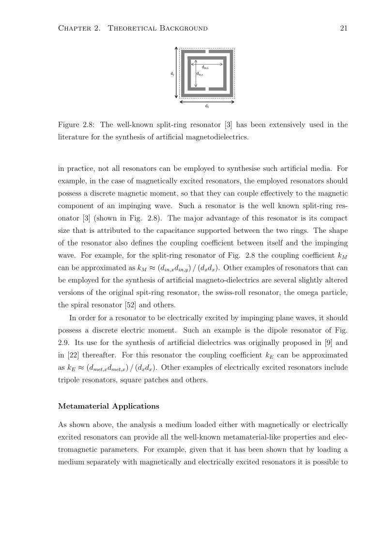
Chapter 2. Theoretical Background 21
dx
dy
din,x
din,y
Figure 2.8: The well-known split-ring resonator [3] has been extensively used in the
literature for the synthesis of artificial magnetodielectrics.
in practice, not all resonators can be employed to synthesise such artificial media. For
example, in the case of magnetically excited resonators, the employed resonators should
possess a discrete magnetic moment, so that they can couple effectively to the magnetic
component of an impinging wave. Such a resonator is the well known split-ring res-
onator [3] (shown in Fig. 2.8). The major advantage of this resonator is its compact
size that is attributed to the capacitance supported between the two rings. The shape
of the resonator also defines the coupling coefficient between itself and the impinging
wave. For example, for the split-ring resonator of Fig. 2.8 the coupling coefficient kM
can be approximated as kM ≈ (din,xdin,y) / (dxdx). Other examples of resonators that can
be employed for the synthesis of artificial magneto-dielectrics are several slightly altered
versions of the original spit-ring resonator, the swiss-roll resonator, the omega particle,
the spiral resonator [52] and others.
In order for a resonator to be electrically excited by impinging plane waves, it should
possess a discrete electric moment. Such an example is the dipole resonator of Fig.
2.9. Its use for the synthesis of artificial dielectrics was originally proposed in [9] and
in [22] thereafter. For this resonator the coupling coefficient kE can be approximated
as kE ≈ (dmet,xdmet,x) / (dxdx). Other examples of electrically excited resonators include
tripole resonators, square patches and others.
Metamaterial Applications
As shown above, the analysis a medium loaded either with magnetically or electrically
excited resonators can provide all the well-known metamaterial-like properties and elec-
tromagnetic parameters. For example, given that it has been shown that by loading a
medium separately with magnetically and electrically excited resonators it is possible to

Chapter 2. Theoretical Background 22
dx
dy
dmet,x
dmet,y
Figure 2.9: The well-known dipole resonator. Arrays of such resonators can be used for
the synthesis of artificial dielectrics.
obtain negative values for the effective magnetic permeability and electric permittivity,
respectively, for a bandwidth just after the self-resonance of the resonators, it is rea-
sonable to suggest that by loading a medium simultaneously with both electrically and
magnetically excited resonators of similar self-resonances, it is possible to achieve a band-
width at which both the effective magnetic permeability and electric permittivity assume
negative values and therefore obtain a left-handed behavior. The equivalent circuit of
such a scenario is depicted in Fig. 2.10.
Besides, in both cases of resonators-loaded media, a stopband is created that is at-
tributed to the negative effective µ or ǫ, obtaining an FSS behavior. Also, in the case of
the magnetically excited resonators, the exhibited effective permeability values before the
self-resonance assume large values even though the loaded medium consists exclusively
of non-magnetic materials. Therefore, such a medium can be employed as an artificial
magneto-dielectric. Finally, given that the effective impedance of any medium is defined
as Zeff =√
µeff/ǫeff , it is clear that both media can be employed for the synthesis
of High-Impedance Structures or, equivalently, Artificial Magnetic Conductors. For the
case of the magnetically excited resonators, this is achieved exactly at or slightly before
the resonance, where the effective permeability assumes very large values. For the case of
the electrically excited resonators, this is achieved exactly at or slight after the frequency
fz at which the effective permittivity becomes zero.
2.1.3 Arrays of Tightly Coupled Resonators
Up to this point, only interaction of resonators with plane waves has been considered,
while any interaction between resonators has been ignored. In this section, the other

Chapter 2. Theoretical Background 23
b)
I1
Ceq
+
-
V1
+
-
V2
I2
Lo,M Cdd
Ldd
kM Co,M
+
-
V1
+
-
V2
I1 I2
IC Io
a)
IC
Leq
Co,E Lo,E
kE
Figure 2.10: Equivalent circuit of a medium loaded with both magnetically and electri-
cally excited resonators. By properly tuning the two resonators, left-handed modes may
be supported by the loaded medium.
extreme scenario is considered. Specifically, it is assumed that the wave propagation is
achieved exclusively through interacting resonators (tightly coupled resonators), in the
absence of free-space propagation. It will be shown that through this approach, a second
class of structures with metamaterial-like properties can be formed.
For this purpose, let us assume an infinite array of ideal, lossless L−C resonators with
resonant frequency ωo = 1/√
LoCo. In the general case, each resonator can be assumed
to be both electrically (capacitively) and magnetically (inductively) coupled with its
adjacent resonators, as in Fig. 2.11, exhibiting a total coupling coefficient k = kE + kM ,
where kE and kM are the electric and magnetic coupling coefficients, given by equations
(2.21) and (2.22), respectively. In the following text, the two extreme cases, in which the
coupling between the resonators is considered either purely electric or purely magnetic,
are examined and the traveling waves supported by such arrays are studied.
kE =
∫ ∫ ∫
ǫ ~E1 · ~E2dυ√
∫ ∫ ∫
ǫ∣
∣
∣
~E1
∣
∣
∣
2
dυ ×∫ ∫ ∫
ǫ∣
∣
∣
~E2
∣
∣
∣
2
dυ
(2.21)
kM =
∫ ∫ ∫
µ ~H1 · ~H2dυ√
∫ ∫ ∫
µ∣
∣
∣
~H1
∣
∣
∣
2
dυ ×∫ ∫ ∫
µ∣
∣
∣
~H2
∣
∣
∣
2
dυ
(2.22)

Chapter 2. Theoretical Background 24
Co Lo Co Lo Co Lo
kE kE kM kM
Figure 2.11: An array of tightly coupled resonators. In the general case, the resonators
may be both electrically (kE) and magnetically (kM) coupled.
2Co
Lo/2 Lo/2
2Co 2Co
Lo/2 Lo/2 Cm
Unit Cell
2Co
Figure 2.12: A unit cell of the array of Fig. 2.11, where the resonators are considered to
be exclusively electrically coupled.
Electrically Coupled Resonators
In the first instance, each resonator of the chain of Fig. 2.11 is assumed to be purely
electrically coupled with its adjacent resonators, i.e. kM = 0, as shown in Fig. 2.12. In
this figure, each resonator has been redrawn as a series connection of two 2Co capacitors
and two Lo/2 inductors, in order to allow for the better representation of the capacitive
coupling between any two adjacent resonators and point out the symmetries in the result-
ing array. The mutual capacitance supported between the electrically coupled resonators
Cm = kE2Co assumes negative values, since the electric coupling coefficient kE, given by
equation (2.21), also assumes negative values. In fact, the sign of kE is defined by the dot
product ~E1 · ~E2. Due to the existence of electric charges, the aforementioned dot product
assumes large negative values if the vectors ~E1 and ~E2 are contra-directional and small
positive values if the vectors ~E1 and ~E2 are co-directional (uncoupled resonators).
The unit cell of Fig. 2.12 has been redrawn in Fig. 2.13, where the coupling mech-
anism is represented with an admittance inverter J = ωCm. Fig. 2.13 can be employed
for the analysis of electrically coupled resonators and the modeling of traveling waves
supported by such arrays. For example, the transmission (ABCD) matrix of the unit
cell can be employed together with Floquet′s theorem, in a similar manner as in [96] and

Chapter 2. Theoretical Background 25
Lo/2 Lo/2
(1-|kE|)2Co
|kE|2Co
(1-|kE|)2Co Vn+1
In In+1
+ +
- -
Vn
Figure 2.13: Equivalent circuit of the unit cell of Fig. 2.12. The coupling mechanism has
been represented with an admittance inverter J = ωCm
[97], to solve for the complex propagation of the waves supported by infinite arrays of
electrically coupled resonators. Specifically, the transmission matrix employed together
with the Floquet′s theorem, as in [96], reads
[
Vn
In
]
=
[
A B
C D
]
UC
·[
Vn+1
In+1
]
=
[
Vn+1eγd
In+1eγd
]
. (2.23)
where γ = α + jβ is the complex propagation constant of the sought traveling waves.
For reciprocal unit cells, equation (2.23) leads to nontrivial solutions of the form
cosh (γd) =AUC + DUC
2(2.24)
Calculating the parameters AUC and DUC for the unit cell of Fig. 2.13 and substitut-
ing them in equation (2.24) leads to the following dispersion relation for the supported
traveling waves:
cosh (γd) = −2Co
Cm
+ ω2Lo
(
(2Co)2 − C2
m
)
2Cm
(2.25)
Given that Cm = − |kE| (2Co) and ωo = 1/√
LoCo, equation (2.25) becomes equivalent
to
cosh (γd) =1
|kE|− ω2
ω2o
1 − |kE|2|kE|
(2.26)
The dispersion relation of equation (2.26) is exclusively depended on the parameters of
each of the resonators and the electric coupling between them. When a purely imaginary
propagation constant is assumed, γ = jβ, equation (2.26) results in dispersion curves
similar with those depicted in Fig. 2.14. These curves correspond to the well-known
forward, slow waves, that have been extensively studied in the past in the context of
filter design. These slow waves are supported within a bandwidth that is defined by the
frequencies flower and fupper (obtained from equation (2.26) for βd = 0, π and given in
equations (2.27) and (2.28), respectively) and depends on the coupling coefficient kE,
according to equation (2.29).

Chapter 2. Theoretical Background 26
0 0.5 1 1.5 2 2.5 32
2.5
3
3.5
4
4.5
5
5.5
6
βd (rad)
Fre
quen
cy (
GH
z)
kE = 0.7
kE = 0.5
kE = 0.3
kE = 0.1
L−L(d=10mm)
Figure 2.14: Dispersion relation (2.26) for different values of the coupling coefficient |kE|.
flower = fo
√
1 − |kE|1 − |kE|2
(2.27)
fupper = fo
√
1 + |kE|1 − |kE|2
(2.28)
∆f
fo
=
√
1 + |kE| −√
1 − |kE|√
1 − |kE|2(2.29)
For ω = ωo, the dispersion relation of equation (2.26) is simplified to cosh (γd) =
kE. Hence, the dispersion equation still depends on the electric coupling between the
resonators. This is the reason why the dispersion curves of Fig. 2.14 do not intersect at
a certain point. Also, in Fig. 2.14 the dotted curve L − L corresponds to the light-line
when periodicity of d = 10 mm is considered.
Magnetically Coupled Resonators
In this section, the resonators that form the array of Fig. 2.11 are assumed to be exclu-
sively magnetically (inductively) coupled, as shown in Fig. 2.15. It will be shown that
this case is much more interesting than the previous one and can lead to much more
interesting results. In Fig. 2.15, the L−C resonators have been redrawn as a series con-
nection of two Lo/2 inductors and two 2Co capacitors, so as to exhibit the symmetries
in the array and show schematically that half of the total inductance of each resonators
is coupled to each of the two adjacent resonators. In that case the mutual inductance

Chapter 2. Theoretical Background 27
Lo/2 Lo/2
2Co 2Co
Lo/2 Lo/2
2Co 2Co Lm
Unit Cell
Figure 2.15: L − C resonators array consisted of magnetically coupled resonators.
kMLo/2
2Co (1-kM)Lo/2 (1-kM)Lo/2 2Co
+
-
+
-
Vn+1
In In+1
Vn
Figure 2.16: Equivalent circuit of the structural unit cell of the magnetically coupled
resonators array. In this unit cell the inductive coupling mechanism is represented with
an equivalent impedance inverter K = ωLm.
between any pair of adjacent resonators is Lm = kMLo/2. The magnetic coupling coeffi-
cient kM , that is given from equation (2.22), assumes both positive and negative values,
due to the non-existence of magnetic charges and because of the fact that the magnetic
fields appear always with closed magnetic lines.
Careful observation of Fig. 2.15 shows that such an array can be created by the
repetition of a structural unit cell that includes the two halves of two adjacent resonators
and the coupling mechanism between them. The exact equivalent circuit of this unit
cell is dependent by both the sign of the magnetic coupling coefficient and the relative
polarity of the coupled inductors. In order, though, to strictly speak about the relative
polarity of two inductors and sign of their coupling coefficient the exact topology of
the inductors should be known. Therefore, a generic equivalent circuit, identical with
that of [32], is employed for the purposes of this analysis. This equivalent circuit cell is
shown in Fig. 2.16. In this equivalent circuit of the unit cell, the coupling mechanism is
represented by an impedance inverter K = ωLm, as also suggested in [32].
Using the unit cell of Fig. 2.16 and equations (2.6) and (2.7), it possible to calculate
the equivalent effective parameters of an 1-D array composed of inductively coupled
resonators. It is pointed out that the extraction of such parameters for a structure that
is composed of tightly coupled resonators and the electromagnetic wave propagation is
exclusively achieved through these resonators (spatial resonances) is not an absolutely

Chapter 2. Theoretical Background 28
rigorous way of modeling since the formed arrays do not constitute an actual medium
and, therefore, can not be described through its effective parameters. Furthermore, the
extraction of the effective parameters for an one-dimensional array can be more effectively
substituted by simply carrying out the dispersion analysis of the periodic structure.
Nevertheless, the effective parameters of the array of inductively coupled resonators are
extracted here in order to point out the nature of the supported propagating waves for
different values and signs of the coupling coefficient kM .
After calculating equations (2.6) and (2.7) for the unit cell of Fig. 2.16, the effective
magnetic permeability and the electric permittivity of the considered arrays of inductively
coupled resonators are found to be
µeff (ω) = −1 − (1 − kM) ω2
ω2o
ω2Cod(2.30)
ǫeff (ω) = − 2
ω2kMLod(2.31)
where Lo, Co and ωo are the self-inductance, self-capacitance and self-resonance of the
considered resonators, kM is the magnetic coupling coefficient, and d is the periodicity
of the array. Equations (2.6) and (2.7) suggest that both µeff (ω) and ǫeff (ω) assume
negative values when kM > 0 for any frequency smaller than fupper, where fupper is
given by equation (2.32). In that case, the supported modes by the examined arrays are
expected to be left-handed or, equivalently, backward-waves .
fupper = fo
1√1 − kM
(2.32)
On the other hand, for negative values of the coupling coefficient (kM < 0), both the
effective constitutive parameters assume positive values for any frequency larger than
flower, where flower is given by equation (2.33). In that case, the corresponding supported
modes are right-handed and the corresponding medium can be considered as an artificial
magnetodielectric.
flower = fo
1√1 + kM
(2.33)
Similar conclusions can be extracted through the dispersion analysis of the unit cell
of Fig. 2.16. Specifically, employing equations (2.23) and (2.24) together with the unit
cell of Fig. 2.16, similar to the case of the electrically coupled resonators, the dispersion
relation for the waves supported by an array of magnetically coupled resonators is found
to be

Chapter 2. Theoretical Background 29
0 0.5 1 1.5 2 2.5 32
2.5
3
3.5
4
4.5
5
5.5
6
βd (rad)
Fre
quen
cy (
GH
z)
kM
= 0.7k
M = 0.5
kM
= 0.3k
M = 0.1
Figure 2.17: Dispersion relation (2.34) for different values of the coupling coefficient |kM |.
cosh (γd) =1
kM
− ω2o
ω2
1
kM
(2.34)
As with the dispersion relation of the electrically coupled resonators, equation (2.34)
depends only on the characteristics of the resonators that comprise the array and the
coupling between them. For positive values of the coupling coefficient kM , the dispersion
equation (2.34) has been plotted in Fig. 2.17, where γ = jβ. This figure validates that
indeed the supported waves by an array of inductively coupled resonators with kM > 0
are backward and the corresponding modes are left-handed.
These modes are supported between the frequencies flower and fupper, as described
above, over a fractional bandwidth that is given by equation (2.35). This equation
suggests that the larger kM is, the larger is the bandwidth of these left-handed modes.
For ω = ωo, the dispersion relation of equation (2.34) is simplified to cosh (γd) = 0,
hence the dispersion equation does not depend on the magnetic coupling between the
resonators. This is the reason why the dispersion curves of Fig. 2.17 intersect at the
point (π/2, ωo) of the dispersion diagram.
∆f
fo
=
√1 + kM −
√1 − kM
√
1 − k2M
(2.35)
Metamaterial Applications
The synthesis of metamaterial structures using tightly coupled resonators has not been
extensively described in the literature. For this reason, a portion of this thesis has been
dedicated to the development of such structures and corresponding antenna applications.

Chapter 2. Theoretical Background 30
Nevertheless, there are two types of already reported metamaterial structures that can
be assumed to be part of this class of metamaterials. The first type of those is the well-
known LC-loaded transmission lines. This type of left-handed media can be considered
as arrays of inductively coupled resonators where kM = 1, suggesting a perfect coupling
between the resonators [98]. The second refers to the magneto-inductive waves that
have been experimentally shown to be supported by arrays composed of large coupled
inductive loops [99], [100].
2.1.4 Discussion
In the theory presented in the previous paragraphs, all the possible ways to synthesise
any of the well-known metamaterial properties were derived through the consideration
of resonators either interacting with impinging plane waves or forming tightly coupled
arrays. Therefore, all the up-to-date proposed metamaterial structures should attribute
their operation either to one of those cases or to a combination of both. In the framework
of this thesis, novel metamaterial structures that rely their operation on the second, least
investigated, case will be developed and studied.
2.2 Periodic FDTD Analysis of Metamaterial Struc-
tures
The theory presented in the previous section of this chapter offers an analytical tool for
the synthesis of any type of metamaterial structure. Nevertheless, it can be employed
only as a first step towards the design or the analysis of a metamaterial structure. For
a more accurate analysis of these structures, a full-wave tool would be required. Given
that metamaterial structures are usually periodic structures, a periodic full-wave compu-
tational tool should be employed for the rigorous and computationally efficient modeling
of metamaterial structures. For this reason, the development of such a tool was consid-
ered extremely important and effort was dedicated to it. Specifically, this tool is a Finite
Difference Time-Domain (FDTD) code that terminated the computational domain with
periodic boundary conditions. Therefore, by simulating a single unit cell of a periodic
structure, the expected response of an infinitely large structure can be obtained. Even
though this tool was initially reported in [93], [95], [92], it has been furthered developed
and optimized for the needs of this thesis and, also, has been extensively employed for

Chapter 2. Theoretical Background 31
the analysis of the metamaterial and metamaterial-inspired structures proposed in this
thesis. Therefore, the theoretical background of the tool is reported in this chapter for
reasons of completeness.
2.2.1 The Finite-Difference Time-Domain Technique
In the FDTD technique, initially proposed by K.S. Yee in 1966 [101], the space for
which Maxwell’s equations have to be solved is properly discretized and all the related
components of the electromagnetic fields are properly located within the formulated
mesh. In turn, time-dependent Maxwell’s equations, in their differential form, are solved
by means of approximative numerical procedures (centered differences), resulting in a
time-marching technique that provides with the temporal evolution of the fields within
the space under consideration.
Although Yee’s algorithm was proposed almost 40 years ago, it was not until the 80′s
that scientists started to further develop it and use it for the modeling of practical appli-
cations. This delay was caused by the lack of computational resources by the time that
the algorithm was initially proposed; the FDTD technique is a computationally demand-
ing technique (in terms of computational memory and power), as Maxwell’s equations
are solved for the whole medium under consideration on a rather dense mesh, in order for
certain conditions, related with the accuracy of the technique, to be satisfied. Therefore,
the development of advanced computational systems was a prerequisite for the further
development and the extended use of the technique.
Maxwell’s Equations in the FDTD Technique
The centered-difference approximation can be used for the solution of the three-dimensional
time-dependent Maxwell’s equations, resulting in a fully explicit, time-stepping, algo-
rithm. Time-dependent Maxwell’s equations, in their differential form, are those of equa-
tions (2.36)-(2.39). Out of these 4 equations, only (2.36)-(2.38) are linearly independent,
while equation (2.39) can be derived using the other three.
∇× E = −∂B
∂t(2.36)
∇× H =∂D
∂t+ JC (2.37)
∇ · E = ρ (2.38)

Chapter 2. Theoretical Background 32
∇ · B = 0 (2.39)
For the needs of the FDTD technique, only equations (2.36) and (2.37) are used, while
it can be shown that equation (2.38) is inherently satisfied for a charge free medium
[1]. Equations (2.36) and (2.37), together with the constitutive relations D = ǫE and
B = µH, can be cast, in rectangular coordinates, for a source free and lossless medium,
in the form:
∂
∂t
Ex
Ey
Ez
=1
ǫ
∂Hz
∂y− ∂Hy
∂z
∂Hx
∂z− ∂Hz
∂x∂Hy
∂x− ∂Hx
∂y
(2.40)
∂
∂t
Hx
Hy
Hz
=1
µ
∂Ey
∂z− ∂Ez
∂y
∂Ez
∂x− ∂Ex
∂z
∂Ex
∂y− ∂Ey
∂x
(2.41)
Then, the problem of the proper discretization of the field components in the three-
dimensional space and time is raised. The best up-to-date solution to this problem has
been proposed by K.S. Yee [101]. According to this solution, the spatial discretization
of the fields should be done according to Fig. 2.18, where the, so-called, Yee’s cell is de-
picted. The first sign for the validity of this discretization scheme is that on the Yee’s cell
each electric/magnetic field component is encircled by all the perpendicular to it mag-
netic/electric, respectively, components, fact that is implied by the Maxwell’s integral
equations. Therefore, in order to apply the centered-differences approximation for the
solution of three-dimensional problems, the space should be discretized using such cubic
unit cells, with dimensions ∆x × ∆y × ∆z, and the field components should be located
on each cell as shown in Fig. 2.18 and extensively presented in Table 2.1. As far as
the discretization in time is concerned, again it is chosen that electric field components
should be sampled at time moments n∆t and the magnetic field components at time
moments (n+ 12)∆t. Hereafter, the points is space and time at which the derivatives will
be approximated have to be properly chosen. As far as the temporal derivatives are con-
cerned, they are calculated at points (n + 12)∆t and n∆t, for the electric and magnetic
field components, respectively. The points at which the spatial derivatives are calcu-
lated are shown in Table 2.2. Finally, equations (2.40) and (2.41) can be approximated,

Chapter 2. Theoretical Background 33
(i,j,k)
(x)
(y)
(z)
Ex
Ex
Ey
Ex
Ez
Ez
Ez
Ey
Ey
Hz
Hy
Hx
Figure 2.18: Yee’s cell.
Field Component Location on Yee’s Space Lattice
Ex (i + 12)∆x, j∆y, k∆z
Ey i∆x, (j + 12)∆y, k∆z
Ez i∆x, j∆y, (k + 12)∆z
Hx i∆x, (j + 12)∆y, (k + 1
2)∆z
Hy (i + 12)∆x, j∆y, (k + 1
2)∆z
Hz (i + 12)∆x, (j + 1
2)∆y, k∆z
Table 2.1: Location of field components on the Yee’s space lattice (according to the
convention of this thesis).

Chapter 2. Theoretical Background 34
∂/∂x ∂/∂y ∂/∂z
Ex (i + 12)∆x, (y + 1
2)∆y, k∆z (i + 1
2)∆x, j∆y, (k + 1
2)∆z
Ey (i + 12)∆x, (j + 1
2)∆y, k∆z i∆x, (j + 1
2)∆y, (k + 1
2)∆z
Ez (i + 12)∆x, j∆y, (k + 1
2)∆z (i + 1
2)∆x, j∆y, (k + 1
2)∆z
Hx i∆x, j∆y, (k + 12)∆z i∆x, (j + 1
2)∆y, k∆z
Hy i∆x, j∆y, (k + 12)∆z (i + 1
2)∆x, j∆y, k∆z
Hz i∆x, (j + 12)∆y, k∆z (i + 1
2)∆x, j∆y, k∆z
Table 2.2: Points on the Yee’s cell at which the partial spatial derivatives of the field
components are calculated (according to the convention of this thesis).
resulting in the following FDTD update equations for the field components:
Ex
∣
∣
n+1
i+ 1
2,j,k
= Ex
∣
∣
n
i+ 1
2,j,k
+∆t
ǫ
Hz
∣
∣
n+ 1
2
i+ 1
2,j+ 1
2,k− Hz
∣
∣
n+ 1
2
i+ 1
2,j− 1
2,k
∆y−
Hy
∣
∣
n+ 1
2
i+ 1
2,j,k+ 1
2
− Hy
∣
∣
n+ 1
2
i+ 1
2,j,k− 1
2
∆z
(2.42)
Ey
∣
∣
n+1
i,j+ 1
2,k
= Ey
∣
∣
n
i,j+ 1
2,k
+∆t
ǫ
Hx
∣
∣
n+ 1
2
i,j+ 1
2,k+ 1
2
− Hx
∣
∣
n+ 1
2
i,j+ 1
2,k− 1
2
∆z−
Hz
∣
∣
n+ 1
2
i+ 1
2,j+ 1
2,k− Hz
∣
∣
n+ 1
2
i− 1
2,j+ 1
2,k
∆x
(2.43)
Ez
∣
∣
n+1
i,j,k+ 1
2
= Ez
∣
∣
n
i,j,k+ 1
2
+∆t
ǫ
Hy
∣
∣
n+ 1
2
i+ 1
2,j,k+ 1
2
− Hy
∣
∣
n+ 1
2
i− 1
2,j,k+ 1
2
∆x−
Hx
∣
∣
n+ 1
2
i,j+ 1
2,k+ 1
2
− Hx
∣
∣
n+ 1
2
i,j− 1
2,k+ 1
2
∆y
(2.44)
Hx
∣
∣
n+ 1
2
i,j+ 1
2,k+ 1
2
= Hx
∣
∣
n− 1
2
i,j+ 1
2,k+ 1
2
+∆t
µ
Ey
∣
∣
n
i,j+ 1
2,k+1
− Ey
∣
∣
n
i,j+ 1
2,k
∆z−
Ez
∣
∣
n
i,j+1,k+ 1
2
− Ez
∣
∣
n
i,j,k+ 1
2
∆y
(2.45)
Hy
∣
∣
n+ 1
2
i+ 1
2,j,k+ 1
2
= Hy
∣
∣
n− 1
2
i+ 1
2,j,k+ 1
2
+∆t
µ
Ez
∣
∣
n
i+1,j,k+ 1
2
− Ez
∣
∣
n
i,j,k+ 1
2
∆x−
Ex
∣
∣
n
i+ 1
2,j,k+1
− Ex
∣
∣
n
i+ 1
2,j,k
∆z
(2.46)
Hz
∣
∣
n+ 1
2
i+ 1
2,j+ 1
2,k
= Hz
∣
∣
n− 1
2
i+ 1
2,j+ 1
2,k
+∆t
µ
Ex
∣
∣
n
i+ 1
2,j+1,k
− Ex
∣
∣
n
i+ 1
2,j,k
∆y−
Ey
∣
∣
n
i+1,j+ 1
2,k− Ey
∣
∣
n
i,j+ 1
2,k
∆x
(2.47)
Up to this point, only isotropic, homogeneous, lossless and source/charge free media
have been assumed. However, the FDTD technique is much more general and can be used
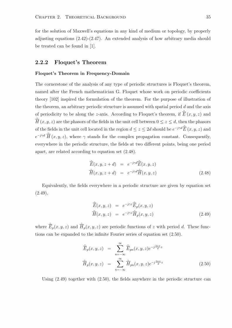
Chapter 2. Theoretical Background 35
for the solution of Maxwell’s equations in any kind of medium or topology, by properly
adjusting equations (2.42)-(2.47). An extended analysis of how arbitrary media should
be treated can be found in [1].
2.2.2 Floquet’s Theorem
Floquet’s Theorem in Frequency-Domain
The cornerstone of the analysis of any type of periodic structures is Floquet’s theorem,
named after the French mathematician G. Floquet whose work on periodic coefficients
theory [102] inspired the formulation of the theorem. For the purpose of illustration of
the theorem, an arbitrary periodic structure is assumed with spatial period d and the axis
of periodicity to be along the z-axis. According to Floquet’s theorem, if E (x, y, z) and
H (x, y, z) are the phasors of the fields in the unit cell between 0 ≤ z ≤ d, then the phasors
of the fields in the unit cell located in the region d ≤ z ≤ 2d should be e−jγdE (x, y, z) and
e−jγd H (x, y, z), where γ stands for the complex propagation constant. Consequently,
everywhere in the periodic structure, the fields at two different points, being one period
apart, are related according to equation set (2.48).
E(x, y, z + d) = e−jγdE(x, y, z)
H(x, y, z + d) = e−jγdH(x, y, z) (2.48)
Equivalently, the fields everywhere in a periodic structure are given by equation set
(2.49),
E(x, y, z) = e−jγzEp(x, y, z)
H(x, y, z) = e−jγzHp(x, y, z) (2.49)
where Ep(x, y, z) and Hp(x, y, z) are periodic functions of z with period d. These func-
tions can be expanded to the infinite Fourier series of equation set (2.50).
Ep(x, y, z) =∞∑
n=−∞
Epn(x, y, z)e−j 2nπd
z
Hp(x, y, z) =∞∑
n=−∞
Hpn(x, y, z)e−j 2nπd
z (2.50)
Using (2.49) together with (2.50), the fields anywhere in the periodic structure can

Chapter 2. Theoretical Background 36
be written as:
E(x, y, z) =∞∑
n=−∞
Epn(x, y, z)e−jγz−j 2nπd
z
H(x, y, z) =∞∑
n=−∞
Hpn(x, y, z)e−jγz−j 2nπd
z (2.51)
Given that the propagation constant γ can be written as γ = β − jα, where α is
the attenuation constant and β the real propagation constant, equation set (2.51) can be
rewritten as:
E(x, y, z) =∞∑
n=−∞
Epn(x, y, z)e−αz−j(β+ 2nπd
)z
H(x, y, z) =∞∑
n=−∞
Hpn(x, y, z)e−αz−j(β+ 2nπd
)z (2.52)
where βn = β + 2nπd
defines all the possibly supported modes (spatial harmonics).
Floquet’s Theorem in Time-Domain
Floquet’s theorem in the form of equation set (2.48) involves the phasors of the fields
(frequency-domain analysis). In order for this theorem to be applied to a time-domain
analysis, it has to be properly expressed in terms of the actual time-varying fields.
In the case of a lossless medium (α = 0), Floquet’s theorem suggests that the fields
at two points, that are one period apart, differ only by the phase factor e−βd. This
phase corresponds to the phase added to a wave after traveling distance d. The proper
interpretation of this statement in time-domain implies that the actual fields, at those
two points, are identical at two time moments which differ by the time interval τd needed
for the wave to travel from the first point to the other (equation set (2.53)).
E(x, y, z, t) = E(x, y, z + d, t + τd)
H(x, y, z + d, t) = H(x, y, z, t − τd) (2.53)
According to equation set (2.53), Floquet’s theorem in time-domain involves both
previous as well as future snapshots of the fields. The time difference between these
snapshots is dependent on the periodicity of the structure and the phase velocity of the
waves in the medium under consideration, and usually is unknown. This interpretation
of Floquet’s theorem suggests that the theorem cannot be used directly in any kind of
time-marching algorithm, as the knowledge of future snapshots of the fields is impossible.

Chapter 2. Theoretical Background 37
FDTD with Periodic Boundary Conditions
Direct Field Methods Field Transformation Methods
Normal Incidence Method Multi-Spatial Grid
Sine-Cosine Method Split-Field
Multiple Unit Cell Methods
Angled Update Method
Table 2.3: Methods that have been proposed for the application of periodic boundary
conditions in time-domain [1].
2.2.3 Periodic Boundary Conditions in the FDTD Technique
General
Floquet’s theorem in the time-domain, as expressed in equation (2.53), can not be used
directly within the FDTD technique, given that this would require the knowledge of
future snapshots of the fields. On the other hand, the existence of several electromag-
netic applications which involve periodic structures and the intense interest for the time-
domain modeling of these structures have motivated researchers to develop techniques
that would overcome this inherent difficulty and allow for the use of Floquet’s theorem
in time-domain analyses. Some of the techniques that have been developed in order to
apply periodic boundary conditions in time-domain are shown in Table 2.2.3. The tech-
niques listed on the right side of Table 2.2.3 are based on a field transformation, used
to overcome the need for time-advanced data, while those listed on the left side provide
ways of directly solving equations (2.42)-(2.47).
Out of these techniques, the one that seems to be more promising for the needs
and the purposes of this thesis is the, so-called, sine-cosine method. This method will
be extensively presented in the next section, while further details about all the other
techniques can be found in [1].
Sine-Cosine Method
The sine-cosine method was initially proposed by Harms et al. [103]. In this method, a
transformation of the Floquet’s theorem is used to overcome the problem of applying the
periodic boundary conditions in time-domain. For the purpose of illustrating the method,
let us assume an arbitrary two-dimensional periodic structure with a direct lattice vector

Chapter 2. Theoretical Background 38
p = dxx + dyy and reciprocal lattice wave vector k = kxx + kyy. In that case, Floquet’s
theorem of equation (2.48) (expressed in frequency-domain), for a point of the structure
r, can be written as follows:
E(r) = E(r + p)e+jk·p (2.54)
H(r + p) = H(r)e−jk·p (2.55)
Assuming that the wave vector k = kxx + kyy corresponds to a wave of frequency ω,
equations (2.54) and (2.55) are equivalent with (2.56) and (2.57), respectively.
E(r)ejωt = E(r + p)e+jk·pejωt (2.56)
H(r + p)ejωt = H(r)e−jk·pejωt (2.57)
Expanding all the exponential factors of equations (2.56) and (2.57), using Euler’s re-
lation, and carrying out some basic algebraic manipulations, equation (2.56) becomes
equivalent with equation set (2.58), while equation (2.57) is equivalent to the equation
set (2.59):
Ecos(r, t) = Ecos(r + p, t)cos(k · p) − Esin(r + p, t)sin(k · p)
Esin(r, t) = Esin(r + p, t)cos(k · p) + Ecos(r + p, t)sin(k · p) (2.58)
Hcos(r + p, t) = Hcos(r, t)cos(k · p) + Hsin(r, t)sin(k · p)
Hsin(r + p, t) = Hsin(r, t)cos(k · p) − Hcos(r, t)sin(k · p) (2.59)
In equation sets (2.58) and (2.59), Ecos(r, t) and Hcos(r, t) stand for the actual
time-varying electric and magnetic fields that possess cosinusoidal time variation1, while
Esin(r, t) and Hsin(r, t) stand for time-varying electric and magnetic fields that possess
sinusoidal time variation2.
Using this transformation, equation sets (2.58) and (2.59), which are equivalent to
Floquet’s theorem of equation (2.48) and its expression in time-domain (equation (2.53)),
are extracted. These equations involve field values which refer exclusively to the same
snapshot. This fact enables the use of periodic boundary conditions, through equation
sets (2.58) and (2.59), within the FDTD technique and the time-domain modeling of
periodic structures.
1Ecos(r, t) = E(r) · cos(ωt) and Hcos(r, t) = H(r) · cos(ωt)2Esin(r, t) = E(r) · sin(ωt) and Hsin(r, t) = H(r) · sin(ωt)

Chapter 2. Theoretical Background 39
Sine-Cosine Method in Practice
In order to illustrate how periodic boundary conditions, through the sine-cosine method,
are applied in practice within the FDTD algorithm, the computational domain of Fig.
2.19 is used. This computational domain can be employed for the modeling of a two-
dimensional periodic structure of a direct lattice vector p = dxx + dyy. In the following,
without loss of generality, only TM waves are assumed and, therefore, only the Ex, Ey
and Hz field components are shown on the computational domain of Fig. 2.19. This
analysis can be easily extended to full three-dimensional cases.
The computational domain of Fig. 2.19 is composed of two grids; the first for the
electric field components (solid line) and the second for the magnetic field components
(dashed line). The dimensions and the location of the electric grid are identical with
the dimensions and the location of the actual physical structure, while the magnetic grid
is half Yee’s cell offset with respect to the electric grid. The location of all the field
components has been chosen in accordance with Table 2.1.
When the computational domain is terminated with periodic boundary conditions,
enforced through the sine-cosine method, the dimensions of the electric and the magnetic
grids have to be identical. In that occasion, the exterior field components of the com-
putational domain are always the electric field components, resulting in a electric grid
which is larger, by one Yee’s cell, than the magnetic grid.
As mentioned in section 2.2.1, the core of the FDTD algorithm is the update equations
(2.42)-(2.47). For those equations to be solved, each electric/magnetic field component
should be encircled by all the perpendicular to it magnetic/electric, respectively, field
components. Going back to the computational domain of Fig. 2.19, it is easy to observe
that the majority of the electric/magnetic field components are encircled by the proper
magnetic/electric field components, so that they can be updated by FDTD equations.
At the same time, this is not the case for certain arrays of grid points. These are the
array of Ex components along the line y = yo, the array of Ey components along the line
x = xo, the array of Hz components along the line y = yo + dy + ∆y/2 and the array
of Hz components along the line x = xo + dx + ∆x/2, as shown in Fig. 2.19. Each of
these arrays is on each of the four exterior boundaries of the rectangular computational
domain. Besides, for all these four grid points arrays, there is the corresponding, parallel
to each of them, array, which is exactly one spatial period (dx or dy) apart. The elements
of the latter grid points arrays can be calculated through Maxwell’s update equations, as

Chapter 2. Theoretical Background 40
(Xo,Yo)
dy
dx
(x)
(y)
Magnetic Field GridElectric Field Grid
HzEyEx
x∆
y∆
Figure 2.19: Computational domain used for the FDTD analysis of a two-dimensional
periodic structure (only TM modes are assumed).
they are composed of field elements that are encircled by the proper field components.
Therefore, it is reasonable to suggest that the elements of each array of the first category
should be updated through the periodic boundary conditions and the use of the field
elements of the arrays of the second category. The pairs of the arrays of field components,
that are updated through the periodic boundary conditions, are summarized in Table 2.4.
After exhibiting how the periodic boundary conditions are applied in space, it remains
to be explained how they will be applied within a time-marching technique. Equation
sets (2.58) and (2.59) involve field snapshots with sinusoidal and cosinusoidal time vari-
ation. Given that a single computational domain could be either exclusively sinusoidally
or cosinusoidally time-varying, it is suggested that two identical computational domains
(e.g. this of Fig. 2.19) should be used for the simulation of a single structure. In the first
one, all the field components will be characterized by a sinusoidal time variation (sine
computational domain) and in the second, all the field components will be characterized
by a cosinusoidal time variation (cosine computational domain). These two computa-
tional domains simulate the same structure, for the wave vector k = kxx + kyy, that
is involved in equation sets 2.58) and (2.59), and run in parallel. The only difference

Chapter 2. Theoretical Background 41
Array of field components Array of field components
updated using Maxwell’s Equations updated using Periodic Boundary Conditions
Ex at y = yo + dy Ex at y = yo
Ey at x = xo + dx Ey at x = xo
Hz at y = yo + ∆y/2 Hz at y = yo + dy + ∆y/2
Hz at x = xo + ∆x/2 Hz at x = xo + dx + ∆x/2
Table 2.4: Pairs of field elements arrays of the computational domain of Fig. 2.19 that
are involved in the application of the periodic boundary conditions.
of these domains is that the excitation of the first is sinusoidally modulated, while the
excitation of the second is cosinusoidally modulated. These two domains interact only
when the periodic boundary conditions of equation sets (2.58) and (2.59) have to be
calculated. It has to be pointed out that, although, these two domains run in parallel
and interact only for the calculation of the periodic boundary conditions, none of them
can produce correct results independently. The whole algorithm for the use of periodic
boundary conditions, through sine-cosine method, in the FDTD technique is shown in
the flow chart of Fig. 2.20.
At this point, the key role of the reciprocal lattice wave vector k = kxx + kyy, which
is involved in equation sets (2.58) and (2.59), should be explicitly discussed. As shown in
the flow chart of Fig. 2.20, the first step of any simulation that involves periodic boundary
conditions, through the sine-cosine method, is the enforcement of a certain value for this
reciprocal lattice wave vector k, both in the sine and the cosine computational domains.
The knowledge of the value of this wave number is a prerequisite for the use of the
algorithm. Therefore, the algorithm calculates the time-domain response of a periodic
medium that corresponds to a certain lattice wave number. This fact imposes a certain
limitation to this type of analysis; each time it is applied to a structure, it solves only
for the waves that correspond to the enforced reciprocal lattice wave vector. Therefore,
in the case that a periodic structure has to be solved for a certain range of wave vectors,
the simulation has to be repeated for all the possible values of the wave vector. The
impact of this limitation to the proposed methodology is reduced by L. Brillouin’s work
on periodic structures [104]. According to this work, for a periodic structure that is
described by a lattice vector p = dxx + dyy, where dx = dy (square unit cell), all the
supported modes are characterized by a wave vector k = kxx+kyy that assumes a limited

Chapter 2. Theoretical Background 42
Cosine Computational Domain
Magnetic field update equations Magnetic field update equations
Periodic Boundary Conditions for the the magnetic field
Electric field update equations Electric field update equations
Set wave vector k
Additional calculations for the electric field(sources, conductors, ABCs, etc)
Additional calculations for the electric field(sources, conductors, ABCs, etc)
Periodic Boundary Conditions for the the electric field
Sine Computational Domain
Figure 2.20: Flow chart of the algorithm that is used for the application of periodic
boundary conditions, through the sine-cosine method, in the FDTD technique.

Chapter 2. Theoretical Background 43
ΓX
M
ky
kx
(y)
(x)
dx
dy
Figure 2.21: Square unit cell (dashed line) and its reciprocal irreducible Brillouin zone
(solid line).
number of values. These values belong to the reciprocal irreducible Brillouin zone on the
k−space. For the case of a two-dimensional periodic structure with square unit cell, the
irreducible Brillouin zone is the triangle ΓXM on the k−space of Fig. 2.21, where Γ
corresponds to the point (kx, ky) = (0, 0), X corresponds to the point (kx, ky) = (π, 0)
and M corresponds to the point (kx, ky) = (π, π).
To conclude this discussion about the way sine-cosine method is applied in practice,
a last comment should be made about the broadband character of the FDTD technique
and whether or not it is affected by the fact that equations (2.56) and (2.57) refer to
monochromatic waves. It has to be pointed out that the periodic boundary conditions of
(2.58) and (2.59) do not affect the broadband characteristics of FDTD. Using arguments
related to Fourier analysis, it can be shown that an analysis that employs equation sets
(2.58) and (2.59) can provide simultaneously with all the supported frequencies (modes)
that correspond to the enforced reciprocal lattice wave vector k = kxx + kyy. This
statement is also supported in [105].
2.2.4 Applications of the Periodic FDTD-based Tool
Dispersion Analysis of Periodic Structures
The first type of analysis that can be performed using the proposed computational tool is
the dispersion analysis of any type of periodic/metamaterial structure. In order for such
an analysis to be carried out successfully, all the modes that can be supported by the

Chapter 2. Theoretical Background 44
structure, for all the wave vectors k = kxx + kyy of the reciprocal irreducible Brillouin
zone on the k-space of Fig. (2.21), have to be detected. This is achieved by enforcing
the aforementioned wave vectors through the periodic boundary conditions and, in turn,
by detecting all the supported resonances through the spectral analysis of the extracted
time-domain responses of the simulated unit cell.
Modal Field Patterns Extraction
Apart from the calculation of the dispersion equations and diagrams of periodic struc-
tures, the proposed methodology can be directly applied to the extraction of the modal
field patterns of the supported modes. These field patterns are calculated from the Fourier
transform of the field components within the FDTD computational domain, iteratively
applied on their time samples. In particular, the Fourier transform of the electric field is
evaluated at a known frequency ω as in equation (2.60),
E (ri,j,k, ω) ≈Ntot∑
n=1
E (ri,j,k, n∆t) × exp(−jωn ∆t) (2.60)
where ri,j,k = x i∆x + y j∆y + z k∆z is the position vector of a FDTD grid point, N the
number of time-steps, counted after the excitation has faded away, used for the Fourier
transform, and E (ri,j,k, n∆t) = Ecos (ri,j,k, n∆t) + jEsin (ri,j,k, n∆t).
Analysis of Leaky-Wave Structures
Finally, the proposed methodology can be employed for the analysis of leaky-wave struc-
tures and the calculation of the complex wave numbers of leaky-waves. The details of
this type of analysis will be presented in details in chapter 6 of this thesis, where this
methodology is developed, optimized and employed for the analysis of several leaky-wave
structures.
2.3 Commercial Electromagnetic Solvers
2.3.1 General
The theory for the synthesis of metamaterial structures considering coupled resonators
and the developed periodic FDTD numerical tool have been extensively used throughout
this thesis, mostly during the initial stages of the analysis and design of novel periodic

Chapter 2. Theoretical Background 45
structures and devices. Nevertheless, many additional commercially available numerical
tools were used for the complete and inclusive characterization of the developed finite-
size structures. These tools are briefly presented in the following text for reasons of
completeness of this theoretical chapter.
2.3.2 Ansoft HFSS
Ansoft HFSS used to be for years the most popular, commercially available, 3-D full-
wave electromagnetic solver. It employs the finite-element-method (FEM) for the solu-
tion of Maxwell’s equation in frequency domain. Ansoft HFSS offers a stable, rigorous,
frequency-domain electromagnetic solver that can be effectively employed for the com-
putationally efficient analysis of complicated structures. It’s comparative advantages are
becoming critical when referring to highly resonant structures, such as filters or meta-
material structures, while its weak points are becoming dominant when referring to the
analysis of broadband structures (frequency sweeping is required for any broadband anal-
ysis). Ansoft HFSS was one of the first commercially available full-wave tools to support
periodic boundary conditions and a periodic (eigenmode) solver. For this reason, HFSS
was used for the validation of the developed periodic FDTD-based tool.
2.3.3 Ansoft Designer
Ansoft Designer is a 2.5-D, method-of-moment (MOM) based electromagnetic tool, capa-
ble of solving Maxwell’s equations in planar electromagnetic structures. Its use becomes
efficient, in terms of the required computational resources and time, when referring to
planar electromagetic structures, such as microstrip-based microwave circuits and an-
tennas. Ansoft Designer also includes a circuit simulator that was used for the circuit
simulations that were required for needs of this thesis.
2.3.4 CST Microwave Studio
CST Microwave Studio (CST MWS) is a relatively new commercial, 3-D full-wave, numer-
ical tool. In its present form, it integrates three different electromagnetic solvers; a finite-
integral time-domain solver, a finite-element frequency-domain solver and a transmission-
line-matrix (TLM) time-domain solver (prior Microstripes solver). The first solver to be
included in CST Microwave Studio was the finite-integral time-domain solver. This solver

Chapter 2. Theoretical Background 46
employs sophisticated, non-orthogonal discretization (meshing) schemes, that allow the
tool to efficiently and rigorously model complicated structures. CST Microwave Studio
offers an extremely convenient and robust graphical user interface that allows for the
accurate and fast insertion of complicated electromagnetic models. Being a time-domain
solver, allows for the broadband analysis of the structures under investigation, while it
becomes inefficient (time-consuming) for highly resonant structures. Nevertheless, for the
analysis of such highly resonant structures, the available frequency-domain solver may
be used. Conclusively, CST Microwave Studio constitutes a robust, rigorous and efficient
computational electromagnetic tool that can be employed for the analysis of almost any
type of electromagnetic problems. This feature together with its excellent graphical user
interface justifies the impressive spread of its use among microwave engineers during the
recent years.

Chapter 3
Spiral-based Artificial Transmission
Lines and Applications
In this chapter, a novel class of uniplanar, fully-printed, microstrip-based artificial lines
supporting backward waves is reported. The synthesis of these lines has been based
on the theory of section 2.1.3 for the synthesis of arrays supporting left-handed modes
considering exclusively inductively tightly coupled resonators. The resonators employed
for the synthesis of the proposed artificial lines are compact, symmetrical, microstrip-
based, fully-printed resonators that possess well-defined inductive characteristics and,
therefore, tend to couple inductively to similar adjacent resonators. These resonators
are explicitly described and modeled in the first section of the chapter. In turn, these
resonators are properly arranged in arrays that support backward waves. Such arrays
are built, measured and characterized at microwave frequencies. Finally, these artificial
lines are employed in the design of series-fed microstrip patch arrays.
3.1 Review of Artificial Transmission Lines
Artificial transmission lines are any engineered transmission lines that apart from the tra-
ditional parameters of conventional transmission lines (characteristic impedance, phase
velocity, time delay) also possess additional features that make them attractive for cer-
tain microwave applications. One of the most popular classes of artificial transmission
lines are the so-called slow-wave transmission lines [32], that exhibit effective refractive
indexes smaller than the unity. In the context of metamaterials and LHM, the first
class of artificial transmission lines was proposed by G.V. Eleftheriades et. al [28] and C.
47

Chapter 3. Spiral-based Artificial Transmission Lines and Applications 48
Caloz et. al [30]. These artificial transmission lines are synthesized by periodically load-
ing conventional transmission lines with series capacitances and shunt inductances, and
exhibit dispersive properties for their effective index of refraction and their characteris-
tic impedance. Following the original implementation of these lines, several alternative
implementations have been proposed in the literature (e.g. [86], [87], [81]).
3.2 Double Spiral Resonators
3.2.1 Description
The fundamental resonator employed in this chapter for the synthesis of the artificial,
fully-printed, microstrip-based left-handed lines is the, so-called, double spiral resonator
(DSR), shown in Fig. 3.1. It is composed of two single spirals that are connected in
series and printed on a grounded dielectric substrate (microstrip-like configuration). This
structure can be assumed to be an alteration of the well-known open-loop resonator (Fig.
3.2), or even the split-ring resonator, towards the direction of enhancing its inductive
components and further minimizing its total size. In its final version, the DSR can be
considered to be composed of two single spirals connected in series. The main reasons
why the DSR has been chosen, in the framework of this project, are its symmetric
properties and the fact that it possesses two discrete and spatially separated magnetic
moments that could be separately coupled to adjacent elements. Even though DSR is not
the most compact resonant element that has been proposed so far in the literature (for
example, the SRR is more compact), for the purposes of this work, these two features
are of much higher importance.
The structure of Fig. 3.1 is an extremely interesting element that could be exploited
both for its inductive and capacitive properties. Therefore, the study of its electro-
magnetic properties in several different configurations (backed on several types of sub-
strates, free standing in the air and others), in accordance with the theory of section 2.1,
could potentially lead to several different metamaterial applications, such as the design
of magneto-dielectrics, EBG structures, LHM, AMC and others. Nevertheless, in the
framework of this thesis, the DSR will be studied exclusive for the case in which they
form arrays of tightly coupled resonators. Furthermore, as far as this chapter of the thesis
is concerned, DSR will be considered exclusively backed on grounded dielectric substrates
(microstrip-like configuration), forming transmission lines that support backward waves.

Chapter 3. Spiral-based Artificial Transmission Lines and Applications 49
dx
dy
(x)
(y)
Figure 3.1: Schematic of a double spiral resonator. In our approach, the spiral is to be
printed on a grounded substrate. The figure should be also assumed to be the computa-
tional domain of the full-wave periodic analysis.
a) b)
Figure 3.2: a) Open-loop resonator. b) Double spiral can be formed by wounding the
open ends of the open-loop resonator.

Chapter 3. Spiral-based Artificial Transmission Lines and Applications 50
3.2.2 Periodic Analysis
As it has been already mentioned in the introduction of the thesis, metamaterials are
periodic structures whose properties are partially attributed to their periodic nature.
Therefore, a periodic analysis of the structural unit cell under consideration should be
always considered as the first step in their analysis. In the following, the double spiral
of Fig. 3.1, backed on a grounded dielectric substrate, will be treated as the structural
unit cell of two-dimensional arrays. The periodicity of these arrays is assumed to be
dx = 6.4mm and dy = 3.2mm, along x− and y−axis, respectively, both the strips width
and the gaps width are s = w = 0.2 mm, while the arrays are built on a substrate of
dielectric constant ǫr = 2.2 and height h = 1.15 mm.
Dispersion Analysis
In order to calculate the modes supported by an array of DSR, the unit cell is anal-
ysed using full-wave simulations with the computational domain being terminated with
periodic boundary conditions. In turn, the frequencies of all the supported modes are
estimated in terms of the phase shift per unit cell of all the Bloch wave-vectors being
within the irreducible Brillouin zone. For the DSR of Fig. 3.1, the calculated dispersion
diagram is shown in Fig. 3.3. These results were extracted using the periodic FDTD
tool presented in section 2.2 and validated (at several points) using Ansoft HFSS.
The results of the dispersion analysis of the DSR show that the first (fundamental)
mode supported by the proposed structure is a backward wave since the corresponding
phase and group velocities are anti-parallel. The formulated passband in which the two-
dimensional structure supports backwards waves extends from approximately 2.5 GHz
to 4 GHz. Specifically for the case that 1-D propagation along x−axis is assumed, the
bandwidth over which backward waves are supported extends from 3.3GHz to 3.9GHz,
a fractional bandwidth of FGW = 17 %. At these frequencies, the total length ℓDblSpiral
of the turns of the double spiral corresponds approximately to the half of the guided
wavelength (ℓDblSpiral = λg/2). Furthermore, the physical dimensions of the unit cell of
Fig. 3.1 are equivalent to λg/12 and λo/16, where λg and λo are the guided and free-
space wavelength of the frequencies within the passband. As a result the medium under
consideration can be treated as an effective dielectric.

Chapter 3. Spiral-based Artificial Transmission Lines and Applications 51
Figure 3.3: Dispersion diagram of the unit cell of Fig. 3.1. The first formulated passband
(fundamental mode) is clearly a backward wave band.
Modal Field Patterns
In order to study the identifying characteristics of the left-handed modes supported by
the double spirals, the in-house FDTD code is employed for the extraction of the modal
field patterns of the major field components of the modes. The periodic FDTD analysis
of the unit cell shows that the identifying components of the electric and magnetic field
that determine the operation of this structure are the electric field components along x−and z− axes and the magnetic field component along z− axis.
In Fig. 3.4, the modal pattern of the Ex field component is plotted for a backward
wave supported at fo = 3.4 GHz and propagating along x−axis (kxdx = π/2,kydy = 0).
This modal field pattern shows that the electric field along x−axis is negligible everywhere
in the unit cell, but the edges of the unit cell and the very middle of the unit cell. These
observations lead to three important conclusions. First, it is shown that between the
adjacent y−oriented metal strips of the spirals the magnitude of the fringing fields are
orders of magnitude below the maximum value of the Ex field component. Therefore,
these strips can be assumed to be coupled under an even-mode excitation (see appendix
A) and no capacitance is developed between them. The same is the situation with the

Chapter 3. Spiral-based Artificial Transmission Lines and Applications 52
x−axis
y−axis
Ex
Figure 3.4: Modal field pattern of the electric field component oriented along x−axis
for the mode that is supported at fo = 3.4 GHz and propagating along x−axis (kxdx =
π/2,kydy = 0).
x−oriented strips of the spiral, conclusion that can be extracted from the observation
of the modal field patterns of the Ey electric field component. The second conclusion
is based on the observation of the very strong Ex component that is supported between
the two adjacent y−oriented strips that belong to the two different single spirals in the
middle of the unit cell. These two strips will be assumed as coupled under an odd-mode
excitation and the supported capacitance between them should be always taken into
account. Last but not least, the Ex field that is supported along y−axis at the edges of
the unit cell (this electric field component is actually supported between two neighboring
unit cells) lead to the conclusion that there is some capacitive coupling supported between
adjacent double spirals.
Fig. 3.5 shows the modal field pattern of the z−oriented component of the electric
field of the same wave as before. The reason why this pattern is presented is to show that
the Ez field component is strong all along the length of the wounded spiral. Therefore, it
can be concluded that all along the length of the spiral a quasi-TEM wave is supported
between the spiral and the ground plane. The same conclusion is supported by obser-
vation of the Hx and Hy modal field patterns, in which the x−oriented component of
the magnetic field assumes large values below the y−oriented strips of the spiral and the
y−oriented component of the magnetic field assumes large values below the x−oriented
strips.

Chapter 3. Spiral-based Artificial Transmission Lines and Applications 53
x−axis
y−axis
Ez
Figure 3.5: Modal field pattern of the electric field component oriented along z−axis for
the mode that is supported at fo = 3.4 GHz and propagating along x−axis (kxdx =
π/2,kydy = 0).
To conclude the analysis of the modal field patterns of the supported backward waves,
the modal pattern of the z−oriented component of the magnetic field is shown in Fig. 3.6.
This pattern suggests that the vertical magnetic field is assumes large values in the middle
of each of the single spirals that compose the double spiral. This field is supported by the
currents on the spirals and suggests that the DSR can support a shunt inductance that
is required for the generation of backward waves, as suggested by Eleftheriades etal. in
[28]. Observation of the phase of the two discrete magnetic components shows that these
are in phase. In an array configuration, these components couple to the corresponding
components of the adjacent DSR, providing the required inductive coupling for the array
to support backward waves.
3.2.3 Equivalent Circuit
In this section, a simplified equivalent circuit for the DSR backed on grounded dielectric
substrates is proposed. This equivalent circuit will be employed in the following text for
the efficient analysis and design of DSR-based artificial transmission lines.

Chapter 3. Spiral-based Artificial Transmission Lines and Applications 54
x−axis
y−axis
Hz
Figure 3.6: Modal field pattern of the magnetic field component oriented along z−axis
for the mode that is supported at fo = 3.4 GHz and propagating along x−axis (kxdx =
π/2,kydy = 0).
Lossless Approach
As it was shown though the extraction of the modal field patterns of the DSR there are
two identifying field components associated with the operation of the DSR; the strong
vertical magnetic field supported by the single spiral resonators and the series capacitance
supported between the two different single spirals of the same DSR. Therefore in the
extraction of the equivalent circuit those two characteristics should be taken into account.
The most simplified equivalent circuit that rigorously and effectively describes all the
electromagnetic properties of the DSR is the one proposed in Fig. 3.7. In this equivalent
circuit, each single spiral is represented with a shunt LC resonator of inductance Lss and
capacitance Css, connected with each other through a series capacitance Cser.
The shunt inductance of each of the single spiral resonators Lss can be calculated
analytically using several different approaches [106], [107], [108]. Most of these models
were compared with each other and were shown to be in good agreement. For the purposes
of this thesis, the inductance of a spiral resonator is calculated using the modified Wheeler
formula proposed in [107]. According to this model, the inductance of a printed spiral
resonator is given by equation (3.1)
Lspiral = K1µ0n2davg
1 + K2ρ(3.1)

Chapter 3. Spiral-based Artificial Transmission Lines and Applications 55
Lss Lss Css Css
Cser
Figure 3.7: Equivalent circuit of the DSR of Fig. 3.1 (lossless case).
where n are the number of the turns of the spiral, davg is the average value of the inner and
outer diameter of the spiral (davg = (din + dout) /2), ρ is the so-called fill ratio of the spiral
defined as ρ = (dout − din) / (dout + din), and the coefficients K1 and K2 are dependent
on the geometry of the spiral under consideration and are reported in [107]. For the case
of the square spiral, K1 and K2 have been found to be 2.34 and 2.75, respectively.
Equation (3.1) estimates the inductance of a printed spiral that is not in close prox-
imity to a ground plane. According to the analysis of [32], when an inductive structure
is in close proximity to a ground plane and a microstrip-like mode is supported, the in-
ductance of the structure in the absence of the ground plane should be corrected by the
factor
Kg = 0.57 −(
0.145 ∗ ℓnw
h
)
(3.2)
in order to account for the presence of the ground plane. In equation (3.2) h is the
distance between the spiral and the ground plane and w stands for the width of the
strips that forms the spirals. Combining equations (3.1) and (3.2), the inductance Lss
involved in the proposed equivalent circuit is given by equation
Lss = KgLspiral. (3.3)
For the single spirals of the DSR of Fig. 3.1, equation (3.3) calculates its inductances
Lss as Lss = 13.78 nH.
The capacitance Css of the single spiral involved in the equivalent circuit of Fig. 3.7
is attributed to both the capacitance supported between the strips that form the spiral
(minor contribution) and the capacitance supported between the strips and the ground
plane (major contribution). The analytical calculation of this parameter in much more
challenging than the calculation of the inductance. Even though there are references in

Chapter 3. Spiral-based Artificial Transmission Lines and Applications 56
Lss Lss
Css Css
Cser
Rss Rss
Figure 3.8: Equivalent circuit of the DSR of Fig. 3.1 (including losses).
the literature that could be employed for this calculation ([107], [108]), it has been seen
that this calculation does not lead to satisfying accurate results and inserts a major error
to the extracted self-resonance of any of the single spirals ωss. For this reason, in the
following analysis, the estimation of the capacitance Css is performed through the full-
wave estimation of the self-resonance of the single spirals. Specifically, the self-resonance
fss of the single spirals is estimated through the full-wave analysis of a weakly excited
single spiral. Then, the capacitance Css is calculated through equation
Css =1
(2πfss)2 Lss
(3.4)
For the single spirals of the DSR of Fig. 3.1, full-wave simulation carried out using
Ansoft Designer estimated the self-resonance of the single spiral to be fss = 5.05 GHz.
Then, equation (3.4) estimates the capacitance Css as Css = 0.072 pF
Finally, the series capacitance Cser involved in the equivalent circuit of Fig. 3.7 can be
considered as the capacitance supported between two strips coupled under an odd mode.
The equations for the calculation of this capacitance are provided in appendix A, and
for the DSR of Fig. 3.1 the series capacitance has been calculated to be Cser = 0.053 pF
Impact of Losses
The equivalent circuit of Fig. 3.7 does not involve any kind of losses. In practice,
however, the operation of the proposed DSR is associated with some ohmic losses that
are attributed mostly to the resistance of the metallic spirals. This resistance can be
represented as an ohmic resistance Rss connected in series with the inductances Lss, as
in Fig. 3.8.

Chapter 3. Spiral-based Artificial Transmission Lines and Applications 57
3.1 3.15 3.2 3.25−55
−50
−45
−40
−35
−30
−25
Frequency (GHz)
Tra
nsm
issi
on (
dB)
Eq. CircuitFull−wave
Figure 3.9: Normalized transmission through a weakly excited DSR calculated using the
equivalent circuit of Fig. 3.8 and Ansoft Designer.
The value of the resistance Rss can be approximated using equation (3.5) [109].
Rss =ℓ
σwδ(
1 − e−tδ
) (3.5)
In equation (3.5), ℓ is again the total length of the strips that form the single spiral
resonators, w is the width of these strips, σ is the conductivity of the metal employed to
print the spirals (in our case copper), δ is the skin-depth of the strips at the frequencies
of interest, and t is the actual thickness of these strips. For the DSR of Fig. 3.1 and for
operation around 3.2 GHz, Rss is approximated as Rss ≈ 1.4 Ω
In order to validate the equivalent circuit of Fig. 3.8 and the approximated associated
parameters, the transmission through a weakly excited DSR, calculated using both the
equivalent circuit of Fig. 3.8 and a full-wave simulation, are compared. For the case
of the results extracted through the equivalent circuit, the equivalent inductors of the
DSR were considered to be weakly coupled to two auxiliary inductors that were directly
connected to the ports of a circuit simulator, while for the case of the full-wave results,
the DSR was excited through two microstrips that were weakly and inductively coupled
to it. Given that for these two cases equivalent coupling coefficients were hard to be
obtained, the magnitudes of the two extracted curves were normalized to each other.
Finally, the results are depicted in Fig. 3.9.
The results of Fig. 3.9 show that the proposed equivalent circuit predicts quite ac-
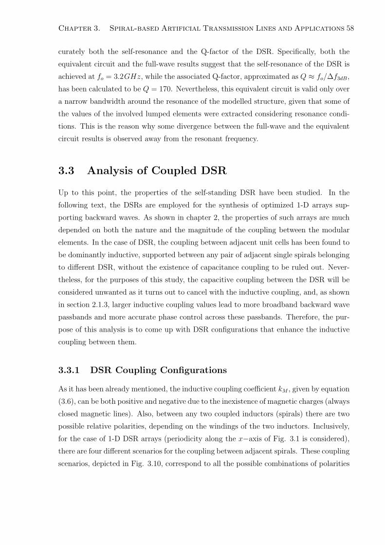
Chapter 3. Spiral-based Artificial Transmission Lines and Applications 58
curately both the self-resonance and the Q-factor of the DSR. Specifically, both the
equivalent circuit and the full-wave results suggest that the self-resonance of the DSR is
achieved at fo = 3.2GHz, while the associated Q-factor, approximated as Q ≈ fo/∆f3dB,
has been calculated to be Q = 170. Nevertheless, this equivalent circuit is valid only over
a narrow bandwidth around the resonance of the modelled structure, given that some of
the values of the involved lumped elements were extracted considering resonance condi-
tions. This is the reason why some divergence between the full-wave and the equivalent
circuit results is observed away from the resonant frequency.
3.3 Analysis of Coupled DSR
Up to this point, the properties of the self-standing DSR have been studied. In the
following text, the DSRs are employed for the synthesis of optimized 1-D arrays sup-
porting backward waves. As shown in chapter 2, the properties of such arrays are much
depended on both the nature and the magnitude of the coupling between the modular
elements. In the case of DSR, the coupling between adjacent unit cells has been found to
be dominantly inductive, supported between any pair of adjacent single spirals belonging
to different DSR, without the existence of capacitance coupling to be ruled out. Never-
theless, for the purposes of this study, the capacitive coupling between the DSR will be
considered unwanted as it turns out to cancel with the inductive coupling, and, as shown
in section 2.1.3, larger inductive coupling values lead to more broadband backward wave
passbands and more accurate phase control across these passbands. Therefore, the pur-
pose of this analysis is to come up with DSR configurations that enhance the inductive
coupling between them.
3.3.1 DSR Coupling Configurations
As it has been already mentioned, the inductive coupling coefficient kM , given by equation
(3.6), can be both positive and negative due to the inexistence of magnetic charges (always
closed magnetic lines). Also, between any two coupled inductors (spirals) there are two
possible relative polarities, depending on the windings of the two inductors. Inclusively,
for the case of 1-D DSR arrays (periodicity along the x−axis of Fig. 3.1 is considered),
there are four different scenarios for the coupling between adjacent spirals. These coupling
scenarios, depicted in Fig. 3.10, correspond to all the possible combinations of polarities

Chapter 3. Spiral-based Artificial Transmission Lines and Applications 59
and signs of the coupling coefficient.
kM =
∫ ∫ ∫
µ ~H1 · ~H2dυ√
∫ ∫ ∫
µ∣
∣
∣
~H1
∣
∣
∣
2
dυ ×∫ ∫ ∫
µ∣
∣
∣
~H2
∣
∣
∣
2
dυ
(3.6)
Specifically, Fig. 3.10(a) and Fig. 3.10(c) depict the case in which the coupled spirals
possess opposite polarities (the left spiral has a clockwise winding and the right spiral
has an anti-clockwise winging). This configuration occurs when the spirals are aligned
symmetrically with respect to the y−axis. Depending on the currents that flow on the
spirals, this configuration may lead to two signs of the coupling coefficient; when currents
are flowing as shown in Fig. 3.10(a) the supported inductive coupling coefficient is nega-
tive (considering that the magnetic lines of each spiral close through its adjacent spiral,
the two magnetic components, where overlapping, are contra-directional and, hence, the
dot product ~H1 · ~H2 is negative). For the same reasons, the inductive coupling coefficient
of the configuration of Fig. 3.10(c) is positive. The lumped-element representations of
the two scenarios are depicted in Fig. 3.10(b) and Fig. 3.10(d), respectively.
Accordingly, the scenarios in which the coupled spirals possess same polarities are
shown in Fig. 3.10(e) and Fig. 3.10(g). For the same reasons as before, the coupling
coefficient in the first of these scenarios will be positive and in the second will be negative.
Artificial lines composed of coupled DSR would not necessarily result in transmission
lines supporting backward waves. On the contrary, as mentioned in chapter 2, the type
of the supported waves will be depending on the sign of the coupling coefficient, or, more
accurately, on the combination of coupling sign and polarity. Specifically, out of the four
scenarios of Fig. 3.10 only two of them will result in backward waves and two of them will
result in forward, right-handed, slow-waves, attributed to an effective high-µ property
(magneto-dielectric). The exact equivalent circuits of these four cases are depicted in Fig.
3.11. The dispersion analysis of all the four equivalent circuits of Fig. 3.11 shows that
the two scenarios that lead to backward waves are the first and the third (Fig. 3.11(a)
and Fig. 3.11(c)) (effective left-handed behaviour) , while those of Fig. 3.11(b) and Fig.
3.11(d) provide solutions only for forward waves (effective magneto-dielectric behavior).
In fact, the cases that lead to backward waves are those that involve shunt inductances
(in Fig. 3.11(a) the equivalent shunt inductance of the coupled spirals is −(− |kM |Lo)
while in Fig. 3.11(c) is (|kM |Lo)).
Given that the purpose of this chapter is the synthesis of artificial lines supporting

Chapter 3. Spiral-based Artificial Transmission Lines and Applications 60
a)
c)
b)
d)
Lss Lss Vn
+
_
In kM < 0
+
_ Vn+1
In+1
Lss Lss Vn
+
_
In kM > 0
+
_ Vn+1
In+1
Opposite Polarity, Negative Coupling
Opposite Polarity, Positive Coupling
Same Polarity, Positive Coupling
Lss Lss
+
_ Vn+1
In+1
Vn
+
_
In kM > 0
e) f)
Same Polarity, Negative Coupling
g)
Lss Lss
+
_ Vn+1
In+1
Vn
+
_
In kM < 0
h)
Figure 3.10: Four possible scenarios and equivalent lumped-element representation for
two inductively coupled spirals, depending on their polarities (windings of the spirals) and
the sign of the coupling coefficient (direction of the flowing currents and the corresponding
magnetic flux).

Chapter 3. Spiral-based Artificial Transmission Lines and Applications 61
a)
b)
Opposite Polarity, Negative Coupling
Opposite Polarity, Positive Coupling
Same Polarity, Positive Coupling
c)
Same Polarity, Negative Coupling
d)
_
In+1
Vn
+
_
2Cser
-Lm Css Css
Lss+Lm Lss+Lm 2Cser
+
In
Vn+1
_
In+1
Vn
+
_
2Cser
-Lm Css Css
Lss+Lm Lss+Lm 2Cser
+
In
Vn+1
_
In+1
Vn
+
_
2Cser
+Lm Css Css
Lss-Lm Lss-Lm 2Cser
+
In
Vn+1
_
In+1
Vn
+
_
2Cser
Lm Css Css
Lss-Lm Lss-Lm 2Cser
+
In
Vn+1
Figure 3.11: Exact equivalent circuits of the four scenarios of Fig. 3.10. For all the
equivalent circuits, regardless of the sign of kM , Lm = kMLo

Chapter 3. Spiral-based Artificial Transmission Lines and Applications 62
backward waves, only the cases of Fig. 3.10(a) and Fig. 3.10(e) will be further investi-
gated. On the other hand, in the following chapters of the thesis, the remaining two cases
will be exploited. Finally, it is clarified that the two coupling scenarios that correspond
to each of the two spirals configurations (polarities) correspond to the two eigensolutions
(modes) of each configuration. Which of the two modes will be established in a certain
application will be depended on the way the spirals are being excited and the surround-
ing electromagnetic environment (boundary conditions). Specifically for the case of the
DSRs-based arrays, it has been seen that the dominant mode is determined by the num-
ber of the DSRs that constitute the array: even number of resonators enhance the modes
that lead to backward waves and odd number of resonators enhance the modes that lead
to forward waves. The latter observation applies exclusively to finite size arrays.
3.3.2 DSR Coupling Assessment
In order to decide which of the two configurations of Fig. 3.10 that lead to backward
waves will be chosen for the synthesis of artificial lines supporting such waves, the coupling
coefficient for the two cases will be calculated. In turn, the configuration that exhibits
larger coupling will be chosen, given that, as shown in chapter 2, larger couplings between
the resonators lead to larger useful bandwidths.
Before proceeding to the rigorous quantitative calculation of the coupling in these two
cases, a comparative estimation for the coupling can be made only by the observation of
Fig. 3.10 and the schematic representation of the currents on this figure. As it has been
mentioned, the coupling between the resonators is mainly inductive and any capacitive
coupling between the DSRs tends to cancel with the inductive coupling, reducing the
total coupling coefficient. The schematic representation of the currents on Fig. 3.10(a)
shows that for this configuration the adjacent strips of the two neighboring spirals are
flown by contra-directional currents (coupled lines under an odd-mode excitation) and,
hence, some coupling capacitance will be supported between them. This capacitance
corresponds to the Ex component that is supported at the edges of the unit cell in the
modal field pattern of Fig. 3.4. Such capacitance is not supported in the configuration
of Fig. 3.10(e), given that the corresponding currents are co-directional. Therefore, it is
expected that the total coupling will be larger for the configuration of Fig. 3.10(e).
For the numerical estimation of the coupling of the two configurations, the well-known
technique of the full-wave simulation of the transmission through pairs of weakly excited

Chapter 3. Spiral-based Artificial Transmission Lines and Applications 63
coupled resonators is employed. Ansoft Designer is used for the full-wave transmission
simulation and the employed models for the two configurations are depicted in Fig. 3.12
and Fig. 3.13, respectively.
Figure 3.12: Ansoft Designer model used for the calculation of the transmission through
a weakly excited pair of coupled DSRs. In this configuration, the double spirals have
been arranged symmetrically along the axis of propagation (as in Fig. 3.10(a) ).
Figure 3.13: Ansoft Designer model used for the calculation of the transmission through
a weakly excited pair of coupled DSRs. In this configuration, the double spirals have
been arranged asymmetrically along the axis of propagation (each spiral is rotated by
180o compared to its adjacent spirals) (as in Fig. 3.10(e) ).
The transmission results obtained for the models of Fig. 3.12 and Fig. 3.13 are
depicted in Fig. 3.14 and Fig. 3.15, respectively. In both cases, the transmission is
maximized at the frequencies f1 and f2, that correspond to the two eigenmodes of each

Chapter 3. Spiral-based Artificial Transmission Lines and Applications 64
configuration. Finally, according to the analysis of [32], the magnitude of the coupling
between the DSR for each configuration is given by equation (3.7).
k =|f 2
1 − f 22 |
f 21 + f 2
2
(3.7)
3 3.1 3.2 3.3 3.4 3.5Frequency (GHz)
Tran
smis
sion
f1
f2
Figure 3.14: Simulated transmission through the weakly excited pair of coupled DSR of
Fig. 3.12.
3 3.1 3.2 3.3 3.4 3.5
Frequency (GHz)
Tran
smis
sion
f1
f2
Figure 3.15: Simulated transmission through the weakly excited pair of coupled DSRs of
Fig. 3.13.
Using the results of Fig. 3.14 and Fig. 3.15 together with equation (3.7), the coupling
coefficient for the configuration of Fig. 3.12 is found to be k = 0.0085 (f1 = 3.175 GHz

Chapter 3. Spiral-based Artificial Transmission Lines and Applications 65
and f2 = 3.23 GHz), while for the configuration of Fig. 3.13 k = 0.035 (f1 = 3.1 GHz
and f2 = 3.31 GHz).
As expected, the total coupling coefficient for the configuration of Fig. 3.13 and Fig.
3.10(e) is larger of that of Fig. 3.12 and Fig. 3.10(a). Therefore, the configuration of
Fig. 3.13 is the one that will be used for the synthesis of 1-D artificial transmission lines
supporting backward waves.
3.4 1-D DSR-based Artificial Transmission Lines
In this section, DSR are employed for the design and fabrication of microstrip-based
transmission lines that support backward waves. Such transmission lines are simulated
and the propagation characteristics are studied. The results of these studies are validated
through the fabrication and measurement of the aforementioned lines. The advantages
of such transmission lines are that these lines are compatible with standard microwave
technologies (microstrip lines), will be fully-printed, and therefore easily fabricated, com-
pletely uniplanar and easily scalable to higher and lower frequencies.
3.4.1 Simulation
Up to this point, the configurations of the DSR along 1-D arrays has been optimized.
What still remains to be identified is the way spiral based transmission lines will be
fed and will match the standard 50 Ω impedance level. It is a common practice, in the
literature, to feed left-handed media using planes waves, properly polarized to excite
the structural elements of the medium. In our case, though, this technique can not be
used given the topology of the medium (printed on a grounded substrate). Furthermore
this technique is usually accompanied by poor transmission through the medium due to
mismatching effects between of the medium with the air.
Therefore a different technique is used to feed the spirals. At the two edges of the
DSR-based transmission lines, single spirals, identical with those that compose the DSR,
properly oriented and perfectly coupled to the adjacent DSR are employed. These single
spirals are open-ended and, therefore, they can be directly attached to a conventional
transmission line. Due to the way the single spirals are located at the edges of the lines
they can be assumed to be part of them. Consequently, these transmission line are fed
by exciting currents directly on them. This is the first time that direct excitation of

Chapter 3. Spiral-based Artificial Transmission Lines and Applications 66
Figure 3.16: Top view of a DSR-based transmission line composed of 4 DSR and embed-
ded within a common 50 Ω microstrip line.
currents on the left-handed medium is reported in the literature to feed such a medium.
Finally, the resulting artificial transmission line is shown in Fig. 3.16.
The simulated S−parameters of the line of Fig. 3.16 are shown in Fig. 3.17. These
results show that the proposed structure exhibit a passband from 3 GHz to 3.4 GHz
(FBW = 13 %), in which the backward waves are supported.
3.4.2 Fabrication and Measurements
In this section, the fabrication and measurement of the transmission line of Fig. 3.16
is reported. The dimensions of each of the DSR that are used are dx = 6.4 mm and
dy = 3.2 mm, while the width of the metallic strips and the gabs between them are g =
s = 0.2mm. The LHM transmission lines are built on RT/duroid5880 dielectric substrate
of dielectric constant ǫr = 2.2 and height h = 1.15mm. The fabricated prototype is shown
in Fig. 3.18. In this prototype six unit cells have been used for the synthesis of the line.
In Fig. 3.19 and Fig. 3.20 the measured and simulated S−parameters of a fabricated
prototype that is composed of four unit cells have been plotted. These figures show
that the fabricated LHM transmission line supports backward waves from 2.9 GHz to
3.3 GHz, a fractional bandwidth of about FBW = 13 %. In this passband, a fairly
satisfying trasmission of −1.8 dB is achieved.
In order to experimentally validate the suggestion that the supported modes in the
formulated passband correspond to backward waves, the inserted phases, by two LHM
transmission lines of different lengths, to a propagating wave are examined. It is well-
known that the difference between these phases are given by equation (3.8), where d1

Chapter 3. Spiral-based Artificial Transmission Lines and Applications 67
Figure 3.17: Simulated S−parameters of the transmission line of Fig. 3.16.
Figure 3.18: Fabricated prototype of a spiral-based transmission line that is composed
of six unit cells.

Chapter 3. Spiral-based Artificial Transmission Lines and Applications 68
2 2.4 2.8 3.2 3.6 4 4.24.2
−25
−20
−15
−10
−5
0
Frequency (GHz)
S11
(dB
)
Measured S11
Simulated S11
Figure 3.19: Measured and simulated S11 of the prototype of Fig. 3.18.
2 2.4 2.8 3.2 3.6 4 4.24.2−70
−60
−50
−40
−30
−20
−10
0
Frequency (GHz)
S21
dB
Measured S21
Simulated S21
Figure 3.20: Measured and simulated S21of the prototype of Fig. 3.18.
and d2 are the lengths of the transmission lines under consideration [110].
∆ϕ = ϕ2 − ϕ1 = −ωn (ω)
c(d2 − d1) (3.8)
Fig. 3.21 shows the measured unwrapped phases that are inserted to a propagating
wave by two of the proposed LHM transmission lines that are composed of four and six
unit cells, respectively. According to these results, the phase inserted by the six unit cells

Chapter 3. Spiral-based Artificial Transmission Lines and Applications 69
2.8 2.9 3 3.1 3.2 3.3 3.40
200
400
600
800
1000
1200
Frequency (GHz)
Unw
rapp
ed T
rans
mis
sion
Pha
ses
(Deg
rees
)
4 Unit Cells
6 Unit Cells
Figure 3.21: Measured unwrapped transmission phases of two DSR-based transmission
lines that are composed of 4 and 6 unit cells, respectively.
line is always greater than this inserted from the four unit cells one. Assuming that d2 is
the total length of the six unit cells and that d1 is the length of the four unit cells, then
∆ϕ > 0, d2 − d1 > 0 and, hence, in order for equation (3.8) to be satisfied, n (ω) must be
negative. Therefore, the effective index of refraction of the proposed transmission lines
is negative.
3.4.3 Impact of Losses
One of the major constraints in the operation of LHM that are composed of highly
resonant metallic particles, such as the SRR or the DSR, is the losses that are inserted
to the waves within the bandwidth of interest. These losses are attributed mostly to
the strong currents that are induced on the metallic elements of the aforementioned
structures at their resonance (ohmic losses). In the following, the nature of these losses
and their impact to the operation of DSR-based transmission lines are studied.
In Fig. 3.22 the simulated power losses across a transmission line that is composed
of four unit cells are plotted for four different cases. In the three of them, the spirals
are assumed to be formed by perfect conductors (σ → ∞), being printed on a substrate
with variable losses. In the fourth case, the spiral are assumed to be printed on a lossless
substrate but using copper (σ = 5.88 ∗ 1007 Siemens/m). For the cases that the losses
of the dielectric substrate are varied (tanδ = 0, 10−4, 10−3) and perfect conductor is
assumed, the power losses across the transmission line are growing as the loss tangent

Chapter 3. Spiral-based Artificial Transmission Lines and Applications 70
2.7 2.8 2.9 3 3.1 3.2 3.3 3.4 3.5 3.60
0.05
0.1
0.15
0.2
0.25
Frequency (GHz)
Pow
er L
osse
s (d
B)
tanδ=0 , Perf. cond.tanδ=0.0001, Perf. cond.tanδ=0.001, Perf. cond.tanδ=0, Copper
Figure 3.22: Simulated power losses across a 4-unit-cell spiral-based transmission line for
several cases of ohmic and dielectric losses.
of the substrate grows, but still assume extremely small values (at the order of 0.05 dB
for a four-cell long line). These values of power losses are of the same order as the losses
that are encountered in the case that no dielectric and conductor losses are assumed
(inherent radiation losses of the structure, at the order of 0.025 dB for a four-cell long
line). Therefore it is concluded that neither the inherent radiation losses of the structure
itself, nor the losses inserted by the dielectric substrate are of critical importance for the
operation of the structure, allowing for the spiral based medium to be printed on cheap
and relatively lossy dielectric substrates (e.g. FR − 4).
On the other hand, the role of the ohmic losses in the operation of this structure is
much more significant. As shown in Fig. 3.22, for the case that conductor losses are
taken into account, the total power losses are significantly large and, specifically, four
times larger than the losses inserted by a substrate of tanδ = 10−3 (worst case scenario
for the dielectric losses). This is due to the strong currents that are developed on the
spirals at their fundamental mode (backward waves modes).
A rough quantitative estimation of ohmic losses, for the structure under consideration,
can be performed by means of the measured transmitted and reflected power. In Fig.
3.23 the total transmitted and reflected power at two LHM transmission lines that are
composed of four and six unit cells is plotted.
Although the exact value of the ohmic losses varies with frequency within the pass-
band (group delay variation), it can be seen that the four unit cells degrade the total

Chapter 3. Spiral-based Artificial Transmission Lines and Applications 71
2.6 2.8 3 3.2 3.4 3.6 3.8−6
−5.6
−5.2
−4.8
−4.4
−4
−3.6
−3.2
−2.8
−2.4
−2
−1.6
−1.2
−0.8
−0.4
00
Frequency (GHz)
S112
+ S
212 (
dB)
4 Unit Cells
6 Unit Cells
Figure 3.23: Measured power losses across a 4-unit-cell and a 6-unit-cell spiral-based
transmission line.
transmitted and reflected power by 1.6 dB, on average, while the six unit cells degrade
the total power by 2.4 dB. Both these observations conclude that each unit cell inserts,
approximately, 0.4 dB power loss. In practice, the actual ohmic power losses per unit
cell are even less since in the estimation of the total losses other sources of power loss,
such as dielectric losses and losses inserted by the connectors, have been included.
3.5 DSR-based Artificial Transmission Lines Appli-
cations
In this section, an application that employs the proposed DSR-based artificial lines is
presented. This application is a series-fed microstrip patch array.
3.5.1 Series-Fed Patch Arrays
General
Series-fed microstrip patch arrays are always good candidates as radiators for applications
that require single-feed, low-profile, fully-printed, highly directive antennas. During the
years, several different series-fed microstrip patch array topologies have been proposed
in the literature. Depending on the specific topology, series-fed arrays can deliver high
directivities in either their E-plane or their H-plane, while, in cases in which both series

Chapter 3. Spiral-based Artificial Transmission Lines and Applications 72
and parallel feeding networks are employed, increased directivities in both the E-plane
and H-plane can be achieved. Furthermore, several studies have been published proposing
techniques for the shaping of the radiated beams. These techniques are mostly employing
the beam shaping possibilities offered by the parameters involved in the array factor of
the array under consideration, i.e. the relative magnitude and phase of the excitations of
each of the elements of the phased array.
In this study, equally spaced, series-fed, microstrip patch arrays that achieve increased
directivity in the E-plane and radiate at broadside are considered. In order for these
arrays to be synthesised, the microstrip patches should be connected in series along their
resonating dimension and be fed in phase. Given the resonant length of each patch
antenna (λg1/2) and that between the radiating edges of each microstrip patch there is
a phase shift of −180o, the interconnecting transmission lines should also insert a phase
shift of 180o between neighboring patches, in order for the latter condition to be fulfilled.
Therefore, conventional microstrip transmission line segments of length λg2/2 should be
used to connect any pair of neighboring patches. Usually, λg1/2 and λg2/2 significantly
differ in length, even though they are referring to the same operating frequency and the
same hosting medium, because of the different widths of the microstrip patches and the
interconnecting transmission lines that result in different effective dielectric constants.
As far as the calculation of the input impedance of such arrays is concerned, it is
possible to assume that both the microstrip patches and the interconnecting transmission
lines act as half-wavelength transformers of the loads that correspond to each of the
radiating edges of the microstrip patches. Therefore the total input impedance of such
array can be assumed, in good proximity, to be equal to the parallel combination of
these loads. In order to get a decent input real impedance, the width of each patch, that
defines the equivalent load of each radiating edge, should be decreased as the number of
the array elements is increased
Proposed study
It is well-known that the directivity of uniformly excited, equally spaced, broadside arrays
depends both on the number of array elements N and the element spacing d. In Fig.
3.24, the analytically calculated directivity of two microstrip patch arrays, composed
of 3 and 4 elements, respectively, as a function of the distance between the edges of
any pair of neighboring array elements, is depicted. For this calculation it has been

Chapter 3. Spiral-based Artificial Transmission Lines and Applications 73
Figure 3.24: Analytically calculated directivity of a three-element and a four-element
microstrip patch array, as a function of the distance between any pair of neighboring
patches.
assumed that the minimum distance between the edges of any pair of neighboring array
elements (0 mm) corresponds to a λg1/2 distance (resonant length of the patch) between
the point radiators for which the array factor has been calculated. As it is shown in
Fig. 3.24, for any given element spacing, the four-element array always achieves higher
directivity (larger effective radiating aperture), while any specific value of directivity
can be achieved by both the three- and four-element arrays, provided that the distance
between the elements is properly set.
As it has been already mentioned, the use of artificial phase-shifting lines allows for
the manipulation of the phase of electromagnetic waves independently of the size of the
structure that supports these waves. In the framework of the uniformly excited, equally
spaced, broadside series-fed arrays, this property could be exploited for the synthesis of
arrays that will be composed of different number of elements but will be able to achieve
the same directivity and occupy the same volume.
Based on this idea, the properties of two different broadside, series-fed arrays, that
are composed of 3 and 4 microstrip patches, respectively, occupy the same volume and
have been designed so as to deliver the same directivity, are compared in this section.
More specifically, the first of these two arrays, shown in Fig. 3.26(a), is composed of
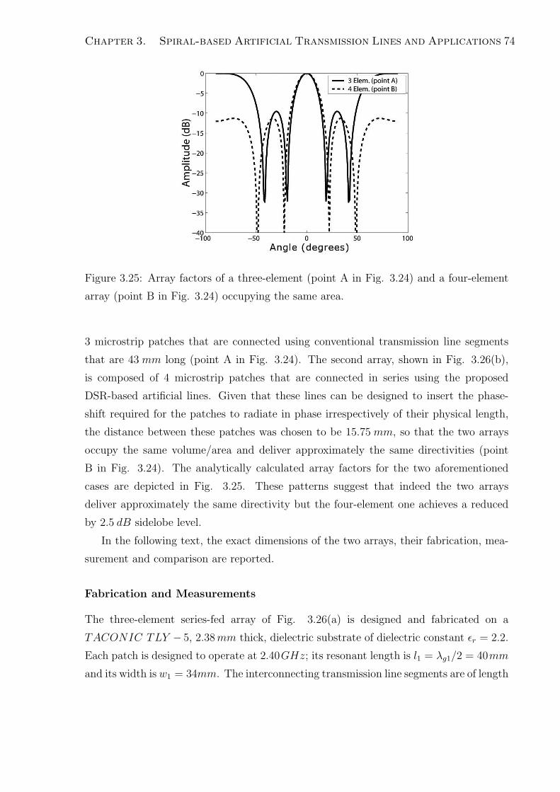
Chapter 3. Spiral-based Artificial Transmission Lines and Applications 74
Figure 3.25: Array factors of a three-element (point A in Fig. 3.24) and a four-element
array (point B in Fig. 3.24) occupying the same area.
3 microstrip patches that are connected using conventional transmission line segments
that are 43 mm long (point A in Fig. 3.24). The second array, shown in Fig. 3.26(b),
is composed of 4 microstrip patches that are connected in series using the proposed
DSR-based artificial lines. Given that these lines can be designed to insert the phase-
shift required for the patches to radiate in phase irrespectively of their physical length,
the distance between these patches was chosen to be 15.75 mm, so that the two arrays
occupy the same volume/area and deliver approximately the same directivities (point
B in Fig. 3.24). The analytically calculated array factors for the two aforementioned
cases are depicted in Fig. 3.25. These patterns suggest that indeed the two arrays
deliver approximately the same directivity but the four-element one achieves a reduced
by 2.5 dB sidelobe level.
In the following text, the exact dimensions of the two arrays, their fabrication, mea-
surement and comparison are reported.
Fabrication and Measurements
The three-element series-fed array of Fig. 3.26(a) is designed and fabricated on a
TACONIC TLY − 5, 2.38 mm thick, dielectric substrate of dielectric constant ǫr = 2.2.
Each patch is designed to operate at 2.40GHz; its resonant length is l1 = λg1/2 = 40mm
and its width is w1 = 34mm. The interconnecting transmission line segments are of length

Chapter 3. Spiral-based Artificial Transmission Lines and Applications 75
b) a)
Figure 3.26: a) Three-element series-fed array, incorporating conventional interconnecting
lines, that corresponds to point A of Fig. 3.24 and b) four-element series-fed array,
incorporating artificial DSR-based interconnecting lines, that corresponds to point B of
Fig. 3.24.

Chapter 3. Spiral-based Artificial Transmission Lines and Applications 76
d1 = λg2/2 = 43 mm (point A in Fig. 3.24) and width 2.0 mm. The total length of the
array is 3l1 + 2d1 = 206.0 mm, while it is fed with a coaxial cable that is attached on the
first element of the array.
The four-element series-fed array of Fig. 3.26(b) is designed and fabricated on the
same dielectric substrate. This array is composed of 4 microstrip patches that are iden-
tical with those employed in the three-element array. The conventional interconnecting
transmission lines of the three-element array have been substituted in this array with
the spiral-based artificial lines. These lines are composed of two DSRs each. The total
physical length of each of the spiral-based lines is d2 = 15.3mm. Each DSR has been de-
signed according to the unit cell of Fig. 3.1, employing 0.35mm wide strips and gaps (to
reduce ohmic losses). In order for the spiral-based artificial line to enforce the elements
of the array to radiate in phase at the targeted operating frequency (2.45 GHz), each
DSR has been designed so as this frequency point to correspond to the +90o phase-shift
point on its dispersion diagram. Finally, the total length of the four-element array is
4l1 + 3d2 = 205.9 mm.A photograph of the two fabricated prototypes is depicted in Fig.
3.27. Both antennas are being fed using a coaxial cable, that is connected to the first
patch through the ground plane and the dielectric substrate.
The measured return loss of the conventional three-element array is presented in Fig.
3.28. These results suggest that the three-element array achieves five different resonances
from 1.9 GHz to 2.9 GHz. The third of them, that supported at 2.40 GHz, is the one at
which the array has be designed to operate. Indeed, this is the resonance that corresponds
to the the case that all the array elements are fed in-phase and the array is radiating
at the broadside direction. The measured −10 dB fractional bandwidth of the antenna
at this frequency is FBW−10 dB = 2.0%. All the other four resonances correspond to
traveling waves that are supported by the array.
The measured return loss of the fabricated four-element array is presented in Fig. 3.29.
These results show that the four-element array exhibits a −10 dB fractional bandwidth
of the order of FBW−10 dB = 15.0% that extends symmetrically around 2.4 GHz. This
bandwidth corresponds to the fractional bandwidth of the employed DSR-based artificial
lines (because of the larger size of the employed DSRs and the higher dielectic substrate,
the bandwidth of these DSRs is larger than those examined in the previous sections of this
chapter). Across that bandwidth of the metamaterial series-fed array multiple resonances
are observed. These resonances are attributed to both the discrete resonances of the 3-
element array, that have been now all included in the operational bandwidth of the
Chapter 3. Spiral-based Artificial Transmission Lines and Applications 77
Figure 3.27: Photograph of the fabricated three- and four-element series-fed array pro-
totypes.
1.5 2 2.5 3−50
−45
−40
−35
−30
−25
−20
−15
−10
−5
0
Frequency (GHz)
|S11
| (dB
)
Figure 3.28: Measured return loss of the conventional three-element array.

Chapter 3. Spiral-based Artificial Transmission Lines and Applications 78
1.5 2 2.5 3−50
−45
−40
−35
−30
−25
−20
−15
−10
−5
0
Frequency (GHz)
|S11
| (dB
)
Figure 3.29: Measured return loss of the four-element array.
4-element array, and the resonances of each of the resonators (spirals) that constitute the
artificial inteconnecting lines. A similar phenomenon (multiple resonances) has been also
observed in [111], where a different class of series-fed arrays with artificial inteconnecting
lines has been investigated.
The E-plane radiation patterns of both the three-element and four-element arrays at
2.4GHz are shown in Fig. 3.30. At this frequency, both arrays exhibit broadside radiation
patterns. The three-element array is slightly more directional than the four-element array,
delivering broadside gain of 11 dBi with a radiation efficiency of approximately 75%. As
far as the four-element array is concerned, it exhibits approximately 2.5 dB reduced
sidelobe levels, as compared to the three-element array, while the delivered gain of this
antenna is 9 dBi and its radiation efficiency approximately 50%. The reduced efficiency
of the four-element array is attributed to the losses on the artificial transmission lines.
Finally, three different E-plane measured radiation patterns of the four-element ar-
ray across its enhanced operating bandwidth are presented in Fig. 3.31. It has been
found that the four-element array scans its main radiating beam with frequency from
the backward direction to the forward direction. Specifically, in Fig. 3.31 the radiation
patterns at frequencies 2.31 GHz, 2.40 GHz and 2.49 GHz are presented. At 2.31 GHz
the four-element array scans its beam at −25o. This beam scans with frequency towards
broadside, where the beam is scanned at 2.40 GHz, and then through broadside towards
positive scanning angles (at 2.49 GHz that beam is scanned at 30o). The efficiency of

Chapter 3. Spiral-based Artificial Transmission Lines and Applications 79
−150 −100 −50 0 50 100 150−40
−35
−30
−25
−20
−15
−10
−5
0
Angle (degrees)
Nor
mal
ized
Am
plitu
de (
dB)
4−element Array3−element Array
Figure 3.30: Measured E-plane radiation patterns of the three-element and four-element
patch arrays at 2.4 GHz.
this antenna across the entire operating bandwidth and all the scanning angles remains
roughly constant. Therefore, the proposed four-element array that employs the artifi-
cial interconnecting lines could be used in application that require beam scanning with
frequency (such as radar applications). The major advantage of the proposed array, as
compared to other metamaterial-based beam-scanning arrays [83], [84], [92], is that it
scans its beam through broadside without any significant reduction of the total achieved
radiation efficiency due to either mismatching effects [92] or increased ohmic losses.

Chapter 3. Spiral-based Artificial Transmission Lines and Applications 80
−150 −100 −50 0 50 100 150−50
−45
−40
−35
−30
−25
−20
−15
−10
−5
0
Angle (degrees)
Nor
mal
ized
Am
plitu
de (
dB)
2.31 GHz2.40 GHz2.49 GHz
Figure 3.31: E-plane radiation patterns of the four-element array at frequencies 2.31GHz,
2.40 GHz and 2.49 GHz.

Chapter 4
A Metamaterial Low-Profile
Monopole-Like Antenna
The analysis, design and measurement of novel, low-profile, small-footprint folded monopoles
employing planar metamaterial phase-shifting lines is presented in this chapter. These
lines are composed of fully-printed spiral elements, that are inductively coupled in order
to exhibit an effective high-µ property. An equivalent circuit for the proposed structure
is presented, validating the operating principles of the antenna and the metamaterial
line. The impact of the antenna profile and the ground plane size on the antenna perfor-
mance are investigated using accurate full-wave simulations. A λ/9 antenna prototype,
designed to operate at 2.36 GHz, is fabricated and tested on both electrically large and
small ground planes, achieving on average 80% radiation efficiency, 5% (110 MHz) and
2.5% (55 MHz) −10 dB measured bandwidths, respectively, and fully omnidirectional,
vertically polarized, monopole-type radiation patterns.
4.1 Introduction
Folded dipoles and monopoles are well-known radiators [112] that provide increased radi-
ation resistance, as compared to the original dipoles and monopoles, while retaining the
same self-resonance. A self-resonant folded monopole of N arms is formed when N − 1
shorted λ/4 monopoles are placed in close proximity to a driven monopole, with the open
ends of all the N wires being connected. At resonance the input radiation resistance of
81

Chapter 4. A Metamaterial Low-Profile Monopole-Like Antenna 82
s << λ/4
h2 << λ/4
Ground Plane Ground Plane
Coaxial Feed
Shorted End
Metamaterial Phase-Shifting
Line
b)
h1 ≈ λ /4
Ground Plane Ground Plane
Coaxial Feed
s << λ/4
Folded Monopole
Shorted End
a)
Low-Profile Folded Monopole
Figure 4.1: Schematic representation of a) the typical folded monopole of height h1 = λ/4
and b) a low-profile folded monopole with an embedded metamaterial phase-shifting line.

Chapter 4. A Metamaterial Low-Profile Monopole-Like Antenna 83
the N -arm folded monopole is
Rrad,fold−mono ≈ N2Rrad,mono (4.1)
where Rrad,mono is the radiation resistance of the single monopole. A coaxially fed folded
monopole composed of two arms is shown in Fig. 4.1(a). The operation of a folded
monopole can be assumed as a superposition of a non-radiating transmission line mode
(contradirectional currents on the wires of the monopole) and an antenna mode (codirec-
tional currents on the wires of the monopole) [112]. The resonance condition of the first
mode is ∆ϕtl = n2π, n = 0,±1,±2... , while the resonance condition for the antenna
mode is ∆ϕant = (n + 1/2)2π, n = 0,±1,±2..., where ∆ϕ denotes the phase shift of
currents flowing between the feeding and the shorting points of the wire that forms the
folded monopole (effective electrical length of the wire). The total current distribution
on a radiating folded monopole is schematically shown in Fig. 4.1(a), suggesting that
the antenna mode becomes dominant.
The radiation resistance of a λ/4 monopole is approximately Rmono = 36.5 Ω. Ac-
cording to equation (4.1), the radiation resistance of the λ/4 folded monopole of Fig.
4.1(a) is expected to be Rfold−mono = 146 Ω. This feature makes the full-length λ/4
folded monopole inappropriate for applications that involve 50Ω feeding lines. Neverthe-
less, the folded monopole configuration has been proved extremely useful in the design
of electrically small antennas that involve low-profile arms with much smaller radiation
resistances than that of the λ/4 monopole. In these cases, the self-resonance of the an-
tenna is secured either by loading the low-profile monopoles with discrete or distributed
inductance (properly meandered radiating wires) or by increasing the monopoles capaci-
tance to the ground. An inclusive study of electrically small folded monopoles, in either
loaded or meandered and multiple-arm configurations, has been presented in [113].
With the advent of metamaterial structures a novel approach for the design of self-
resonant, low-profile folded monopoles has been proposed, originally in [114], [115], [116]
and very recently in [117]. According to this approach, the use of sub-wavelength meta-
material phase-shifting lines is exploited in order to connect the radiating posts of the
folded monopoles and satisfy a self-resonance condition, as shown in Fig. 4.1(b). Specif-
ically, in the antenna designs of [114], [115], [116], [117] different numbers of radiating
posts have been connected through zero-degree phase-shifting L − C loaded transmis-
sion lines that enforce the posts to radiate in-phase, resulting in a folded-monopole-like
behavior.

Chapter 4. A Metamaterial Low-Profile Monopole-Like Antenna 84
In the present chapter, a new approach for the design of self-resonant, low-profile
folded monopoles is reported. In this approach, the use of subwavelength metamaterial
phase-shifting lines is exploited in order to connect the radiating low-profile posts of
two-arm folded monopoles and enforce the actual resonance condition of the supported
antenna mode. In the proposed antenna design, the phase-shifting line is implemented
through a single line that is composed of fully-printed, inductively coupled resonators that
synthesise a medium supporting mostly slow waves and characterized by an effective high-
µ property. In fact, the embedded phase-shifting lines are employed in order to insert the
phase-shift required to be added to the phase of the currents flowing on the radiating,
low-profile posts in order for the resonance condition of the antenna mode ∆ϕant = π to
be established between the feeding and shorting points, in contrast to the antenna designs
of [114], [115], [116], [117] in which the metamaterial phase-shifting lines were employed
to insert a zero-degree phase shift and enforce the radiating posts to radiate in-phase. As
compared to the folded monopoles investigated in [113], the proposed low-profile folded
monopoles do not require any loading with discrete elements (lumped inductors), do not
involve any meandered radiating wires (that may impose difficulties in the fabrication
procedure), and exhibit much smaller footprint than that of the capacitively loaded
monopoles.
A general description of the proposed class of self-resonant, coaxially-fed low-profile
folded monopoles is presented in section 4.2 of the chapter. A detailed description of the
employed phase-shifting lines and their operation when embedded within the proposed
folded monopoles is presented in section 4.3, while a simplified equivalent circuit for the
proposed antenna is presented in section 4.4. Subsequently, an initial implementation
of the proposed low-profile folded monopole, designed to operate at 2.4 GHz and built
on an electrically large ground plane, together with simulated and measured results are
reported in section 4.5. In section 4.6, it is shown that the employed phase-shifting lines
can be used to enforce the antenna mode irrespectively of the profile of the radiating posts
and the radiation properties of ultra low-profile folded monopoles are investigated. In
section 4.7, the impact of the ground plane against which the proposed antennas are built
is examined. Based on the results of this study, the measurement of two optimal antenna
designs are reported in the same section. In section 4.8 a microstrip-fed version of the
proposed antenna is presented and, finally, in section 4.9 the electromagnetic coupling
between pairs of the proposed antenna is assessed.

Chapter 4. A Metamaterial Low-Profile Monopole-Like Antenna 85
4.2 Proposed Antenna Design - General Description
A general description of the proposed antenna design that effectively implements the
antenna model of Fig. 4.1(b) is reported in this section. The side view of the proposed
antenna is depicted in Fig. 4.2(a). As shown in Fig. 4.2(a), the antenna is mainly
composed of two vertical posts, that constitute the main radiation mechanism of the
antenna. The bottom of the first post is directly connected to a feeding port that is a
coaxial cable in this case (feeding post). The second post is connected directly to the
ground plane against which the antenna is fed, at an electrically small distance from
the first post, similarly with the folded monopoles of Fig. 4.1 (shorting post). These
two posts are connected through a spiral-based, metamaterial, phase-shifting line that is
presented in detail in the next section. In the space around these two posts, three layers
of different materials are present. Two of them, these represented with grey color in
Fig. 4.2(a), are dielectric substrates of dielectric constant ǫr and heights hsub1 and hsub2,
that are used in order to bear the ground plane against which the antenna is fed and
the printed metamaterial phase-shifting line, respectively. The space between these two
substrates is filled with air or any other material with dielectric constant close to that of
the free space ǫ0 (e.g. Rohacell foam) that can be employed to hold the two substrates
apart at a certain distance hair. The total profile of the antenna is h = hsub1+hair +hsub2.
The top view of the proposed antenna is shown in Fig. 4.2(b). It mainly depicts
the metalization that is printed on the top side of the upper dielectric substrate of
Fig. 4.2(a). The metalization is composed of two square pads that directly load the
two posts, and the employed metamaterial phase-shifting line that is composed of two
inductively coupled spiral resonators directly attached to the square pads. The operation
of the phase-shifting line will be explicitly explained in the following section. The total
dimensions of the metalization printed on the top side of the upper dielectric substrate
are dx,total × dy,total. For the cases that will be discussed in the following text, these
dimensions are always much smaller than the operating wavelength (dx,total, dy,total << λ),
ensuring that the employed metamaterial phase-shifting line is always of subwavelength
dimensions and the two vertical posts are separated by a subwavelength distance. In
contrast to all the antenna designs investigated in [113], in the proposed antenna design
there is no dc connection between the two vertical posts. The latter feature, apart from
being a major differentiator of the proposed antenna, could be potentially exploited
for the design of easily fabricated reconfigurable monopoles. Such reconfigurable folded
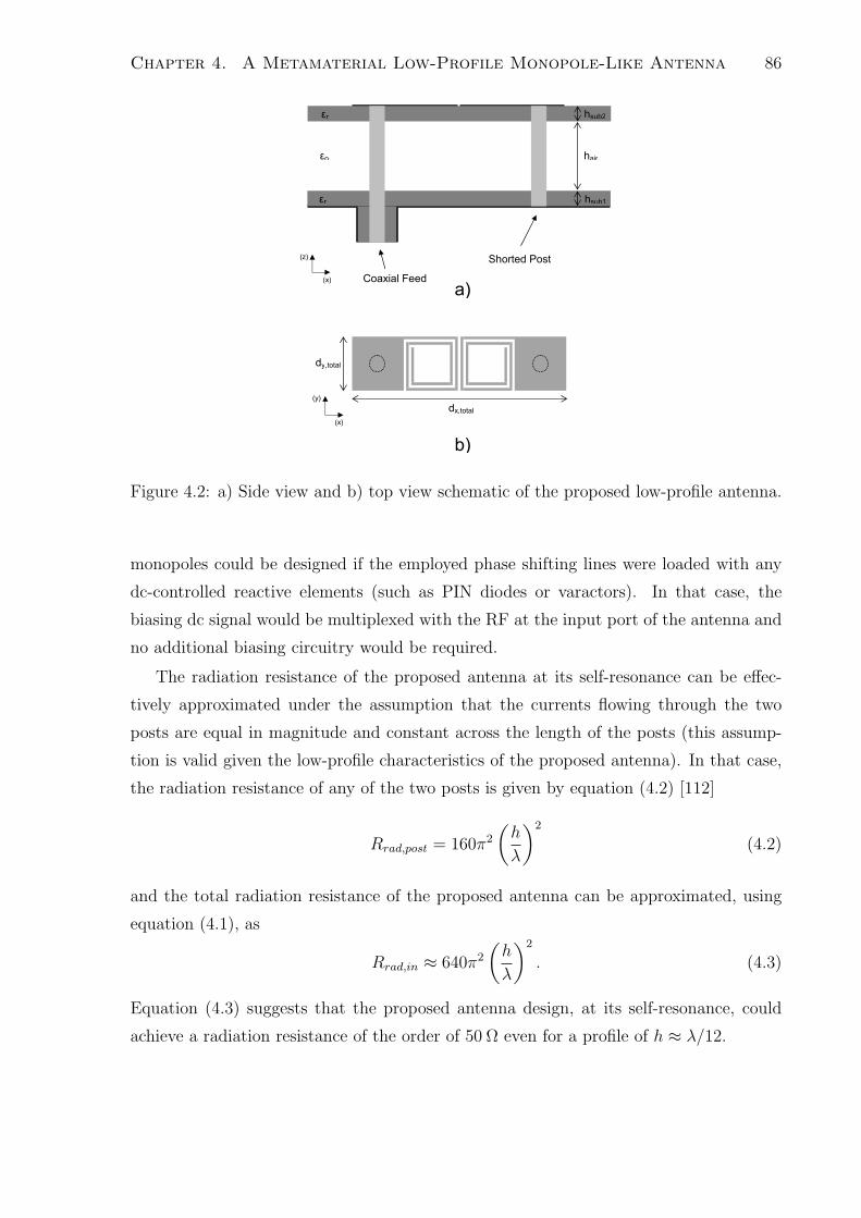
Chapter 4. A Metamaterial Low-Profile Monopole-Like Antenna 86
(z)
(x)
εr
εr
εo
hsub1
hsub2
hair
Coaxial Feed
Shorted Post
(x)
(y)
dy,total
dx,total
a)
b)
Figure 4.2: a) Side view and b) top view schematic of the proposed low-profile antenna.
monopoles could be designed if the employed phase shifting lines were loaded with any
dc-controlled reactive elements (such as PIN diodes or varactors). In that case, the
biasing dc signal would be multiplexed with the RF at the input port of the antenna and
no additional biasing circuitry would be required.
The radiation resistance of the proposed antenna at its self-resonance can be effec-
tively approximated under the assumption that the currents flowing through the two
posts are equal in magnitude and constant across the length of the posts (this assump-
tion is valid given the low-profile characteristics of the proposed antenna). In that case,
the radiation resistance of any of the two posts is given by equation (4.2) [112]
Rrad,post = 160π2
(
h
λ
)2
(4.2)
and the total radiation resistance of the proposed antenna can be approximated, using
equation (4.1), as
Rrad,in ≈ 640π2
(
h
λ
)2
. (4.3)
Equation (4.3) suggests that the proposed antenna design, at its self-resonance, could
achieve a radiation resistance of the order of 50 Ω even for a profile of h ≈ λ/12.

Chapter 4. A Metamaterial Low-Profile Monopole-Like Antenna 87
dx
dy
a)
dx
b)
dy
w
s
Figure 4.3: Unit cell of a) a free standing DSR and b) a DSR participating in an array.
4.3 Spiral-Based Phase-Shifting Lines
An antenna design similar to the low-profile folded monopole of Fig. 4.1(b) requires
a metamaterial phase-shifting line that would be compact (s << λ/4), non-radiating,
and preferably planar, fully-printed and low-loss. It is reminded at this point that the
purpose of this phase-shifting line is to add the required phase in order for the flowing
on the radiating posts currents to satisfy the resonance condition of the antenna mode of
a typical folded monopole (∆ϕant = π). For the design of such a phase-shifting line, the
use of tightly coupled resonators can be considered. Nevertheless, for this application,
the wanted supported mode is not the backward wave mode discussed in chapter 3, but
a slow wave mode instead.
For the implementation of the required slow waves, the use of the DSR, similar with
that of Fig. 4.3(a), is also proposed. Nevertheless, in this case different polarities, as
compared to these considered in chapter 3, between adjacent spirals will be required
to achieve the required operating mode. Specifically, the relative polarities of adjacent
tightly coupled spirals in this case will be similar with that depicted in Fig. 4.3(b).
The equivalent circuit of the DSR of Fig. 4.3(a) is depicted in Fig. 4.4(a), while
that of the configuration of Fig. 4.3(b) is depicted in Fig. 4.4(b). For a DSR employed

Chapter 4. A Metamaterial Low-Profile Monopole-Like Antenna 88
Css
Lss
2Cser
Css
2Cser
Lss
b)
kM
+ +
_ _
V1 V2
I1 I2
Lss Lss Css Css
Cser
a)
Figure 4.4: Equivalent circuit representation of the unit cells of a) Fig. 4.3(a) and b)
Fig. 4.3(b).
in a non-grounded configuration, printed on a substrate of dielectric constant ǫr = 2.2,
and designed to operate at the 2.4 GHz band, with dx = 8.2 mm, dy = 3.8 mm and
w = s = 0.2 mm, the involved equivalent circuit parameters have been found to be
Lss = 24.8 nH, Css = 0.085 pF and Cser = 0.06 pF .
For reasons of completeness, it is reminded that, in the general case, the periodic
analysis of the configuration of Fig. 4.3(b) and the equivalent circuit of Fig. 4.4(b) can
provide non-trivial solutions both for backward and forward slow waves, depending on the
sign of the coupling coefficient kM (as also shown in Fig. 4.5 and Fig. 4.6). Nevertheless,
the specific configuration secures an optimized (maximized) positive coupling coefficient
that enables the forward slow waves to become dominant.
Finally, in order to quantify the propagation characteristics along a single unit cell
identical with that of Fig. 4.3(b), its transmission magnitude and phase, obtained
through the analysis of the equivalent circuit of Fig. 4.4(b), are presented in Fig. 4.7.
These results suggest that the single unit cell exhibit satisfying transmission for all the
points of its dispersion curve. Across this bandwidth, the single unit cell could provide
any phase-shift between 0o and −180o. Therefore, the single unit cell of Fig. 4.3(b) could
be used as phase-shifting line for the proposed low-profile folded monopole of Fig. 4.1(b).

Chapter 4. A Metamaterial Low-Profile Monopole-Like Antenna 89
V1 +
_ _
2Cser
Lm Css Css
Lss-Lm Lss-Lm 2Cser
+
I1
a)
c)
b)
d)
kM <0
kM >0
V2
I2
V1 +
_ _
2Cser
-Lm Css Css
Lss+Lm Lss+Lm 2Cser
+
I1
I2
V2
Figure 4.5: Coupling scenarios for a pair of spirals and equivalent circuit representations.
Lss corresponds to the self-inductance of each of the spirals and Lm = |kM |Lss to the
absolute value of their mutual inductance.
0 0.5 1 1.5 2 2.5 30
0.5
1
1.5
2
2.5
3
βd (Radians)
Fre
quen
cy (
GH
z)
kM
< 0 k
M > 0
Light−line
Figure 4.6: Dispersion curves of the unit cell of Fig. 4.4(b) for positive and negative
values of the coupling coefficient kM .
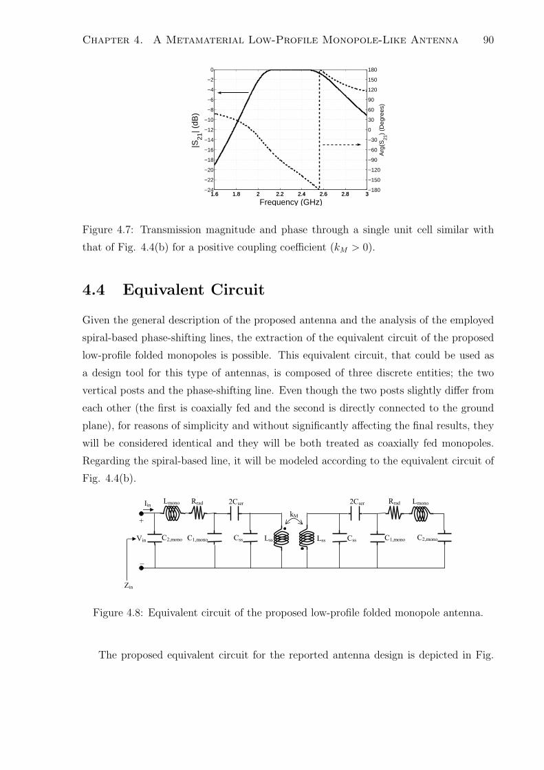
Chapter 4. A Metamaterial Low-Profile Monopole-Like Antenna 90
1.6 1.8 2 2.2 2.4 2.6 2.8 3−24
−22
−20
−18
−16
−14
−12
−10
−8
−6
−4
−2
0
|S21
| (dB
)1.6 1.8 2 2.2 2.4 2.6 2.8 3
−180
−150
−120
−90
−60
−30
0
30
60
90
120
150
180
Frequency (GHz)
Arg
(S21
) (D
egre
es)
Figure 4.7: Transmission magnitude and phase through a single unit cell similar with
that of Fig. 4.4(b) for a positive coupling coefficient (kM > 0).
4.4 Equivalent Circuit
Given the general description of the proposed antenna and the analysis of the employed
spiral-based phase-shifting lines, the extraction of the equivalent circuit of the proposed
low-profile folded monopoles is possible. This equivalent circuit, that could be used as
a design tool for this type of antennas, is composed of three discrete entities; the two
vertical posts and the phase-shifting line. Even though the two posts slightly differ from
each other (the first is coaxially fed and the second is directly connected to the ground
plane), for reasons of simplicity and without significantly affecting the final results, they
will be considered identical and they will be both treated as coaxially fed monopoles.
Regarding the spiral-based line, it will be modeled according to the equivalent circuit of
Fig. 4.4(b).
Lss C1,mono C2,mono Css Lss Css C2,mono C1,mono
Lmono Rrad
Zin
2Cser
kM
2Cser Rrad Lmono
Vin
+
_
Iin
Figure 4.8: Equivalent circuit of the proposed low-profile folded monopole antenna.
The proposed equivalent circuit for the reported antenna design is depicted in Fig.

Chapter 4. A Metamaterial Low-Profile Monopole-Like Antenna 91
4.8. The first and the last parts of the proposed equivalent circuit correspond to the
two vertical monopoles. The inductance Lmono of the two posts depends on their length
and their radius and can be calculated, assuming the quasi-static analysis of [106], using
equation (4.4).
L mono = 0.2 · h ·[
ℓn
(
4h
dpost
)
− 3
4
]
[nH] . (4.4)
Assuming that the vertical posts are lossless, the only resistive component involved
in their equivalent circuit is their radiation resistance Rrad. The radiation resistance
of each post can be calculated, when considering it to be short and be driven by a
constant current, using equation (4.2). Finally, the capacitances C1,mono and C2,mono
involved in the equivalent circuit of Fig. 4.8 represent the internal capacitance of each
monopole, that defines together with Lmono the input impedance and the self-resonances
of the monopole, and its external capacitance, that is encountered when a monopole is
fed coaxially against a ground plane, respectively. These capacitances depend on the
loading of each of the posts (surrounding dielectric material, loading pads etc) and the
most effective way to be calculated are through the full-wave simulation of the coaxially
fed short monopole and the full-wave estimation of its self-resonance ωres and its anti-
resonance ωanti−res. Specifically, given that the series branch Lmono −C1,mono defines the
resonance of the monopole and the parallel combination of the branch Lmono − C1,mono
with the capacitance C1,mono defines its anti-resonance, the capacitances C1,mono and
C2,mono can be approximated, when ωres and ωanti−res have been estimated through a
full-wave simulation, using equations (4.5) and (4.6), respectively.
C1,mono ≈1
ω2resLmono
(4.5)
C2,mono ≈C1,mono
ω2anti−resLmonoC1,mono − 1
(4.6)
The remaining lumped elements involved in the equivalent circuit of Fig. 4.8 refer
to the employed phase-shifting line. Both the impact and the way their values can be
estimated have been reported in section 4.3. Therefore, the only parameter involved in
the equivalent circuit that remains to be quantified is the inductive coupling coefficient
kM . According to [32], when the transmission through a weakly excited pair of coupled
resonators is known, the coupling coefficient can be calculated using equation
kM =f 2
2 − f 21
f 22 + f 2
1
, (4.7)

Chapter 4. A Metamaterial Low-Profile Monopole-Like Antenna 92
where f1 and f2 are the two resonances of the coupled configuration (frequencies at
which the transmission through the coupled pair is maximized). At these frequencies
the transmission phase sign is altered. Consequently, in cases that only the transmission
through a strongly excited pair is known, as in Fig. 4.7, the coupling coefficient can
be approximated by calculating equation (4.7) for two frequencies that correspond to
transmission phases that differ by 180o.
Considering the antenna model of section 4.2 with a profile of λ/9 and the spiral
dimensions reported in section 4.3, the parameters of the presented equivalent circuit
assume the following values; for the short monopoles Lmono = 9.3 nH, Rrad = 19 Ω,
C1,mono = 0.25 pF and C2,mono = 0.29 pF , and for the metamaterial phase-shifting line
Lss = 24.8 nH, Css = 0.081 pF , Cser = 0.06 pF and kM = 0.2. It is pointed out that
all the values of the parameters associated with the operation of the phase-shifting line
are dependent on the distance of the line from the employed ground plane. Therefore,
different antenna profiles will result in different values for these parameters.
The input impedance of the considered λ/9 antenna design, calculated using the
proposed equivalent circuit and also using a full-wave Ansoft HFSS simulation, is shown
in Fig. 4.9 and Fig. 4.10. The equivalent circuit results are in good agreement with
the full-wave results. The major disagreement between them concerns the values of the
calculated impedance around the anti-resonances of the structure. This disagreement
should be attributed to the modeling of the posts and the phase-shifting line as lossless
structures and also to the fact that the two posts were considered identical. However,
good agreement is achieved for the resonances that are of our interest.
4.5 Low-Profile Antenna at 2.4 GHz
4.5.1 Antenna Parameters and Full-wave Simulations
The parameters that were considered in the previous sections for the profile of the folded
monopole and the dimensions of the spirals are used in this section for the simulation
and fabrication of an initial prototype of the proposed low-profile antenna that would
operate at approximately 2.4 GHz. The profile of this initial antenna prototype has
been chosen to be approximately λ/9 in order to ensure that, according to equation
(4.3), the antenna prototype would exhibit a decent radiation resistance (≈ 50 Ω) and,
therefore, could be easily matched to a 50 Ω feeding port (SMA connector). This λ/9

Chapter 4. A Metamaterial Low-Profile Monopole-Like Antenna 93
1.8 2 2.2 2.4 2.60
500
1000
1500
2000
2500
3000
Frequency (GHz)
Inpu
t Res
ista
nce
(Ohm
s)
Full−waveEq. Circuit
Figure 4.9: Input resistance of the antenna of section 4.2 calculated using the equivalent
circuit of Fig. 4.8 and Ansoft HFSS simulations.
1.7 1.8 1.9 2 2.1 2.2 2.3 2.4 2.5 2.6 2.7−1500
−1000
−500
0
500
1000
1500
Frequency (GHz)
Inpu
t Rea
ctan
ce (
Ohm
s)
Full−waveEq. Circuit
Figure 4.10: Input reactance of the antenna of section 4.2 calculated using the equivalent
circuit of Fig. 4.8 and Ansoft HFSS simulations.
monopole is initially built on an electrically large ground plane (the employed ground
plane dimensions are 2λ × 2λ). At the targeted operating frequency the wavelength is
λ = 125 mm. In order to achieve an antenna profile of h = λ/9, the length of the
employed posts is set to be hpost = hsub1 + hair + hsub2 = 13.8 mm. The diameter of the
posts is dpost = 0.91 mm. This dimension is mainly enforced by fabrication restrictions
(core wire of the used coaxial cable). The employed dielectric substrates are of dielectric
constant ǫr = 2.2 and height hsub1 = hsub2 = 2.4 mm. Therefore, the distance between
the two substrates is set to be, in this initial design, hair = 9.0 mm. Referring to

Chapter 4. A Metamaterial Low-Profile Monopole-Like Antenna 94
the top view of the reported design (Fig. 4.2(b)), the total footprint of the antenna is
dx,total × dy,total = 15.8 mm × 3.8 mm ≈ λ/8 × λ/33. The square pads that directly load
the posts are of dimensions 3.8 mm × 3.8 mm.
As far as the metamaterial phase-shifting line is concerned, the double spiral res-
onators are designed to achieve their first self-resonance (half-wavelength resonators) at
2.34 GHz, when placed 13.8 mm above a ground plane and in the presence of all the
dielectric layers of Fig. 4.2(a). Referring to Fig. 4.3, this is achieved when dx = 8.2 mm,
dy = 3.8 mm and the width of the strips and the gaps between them is set to be
w = s = 0.2 mm. The transmission characteristics of this specific phase-shifting line
have been already presented in Fig. 4.7.
The proposed antenna was simulated using Ansoft HFSS. The simulated input impedance
of the λ/9 antenna design is depicted in Fig. 4.11. This result suggests that the pro-
posed structure achieves its first self-resonance (Xin (ω) = 0 and ∂Xin (ω) /∂ω > 0) at
1.8 GHz. Even though this frequency is out of the band of operation of the employed
phase-shifting line (Fig. 4.7), there is some wave transmission through the spirals at this
frequency, with a positive phase-shift added to the transmitted waves (assuming that
negative phase is added to a forward propagating wave). In fact, what occurs at 1.8GHz
is that the phase-shifting line compensates the negative phase-shift added to the currents
when flowing on the radiating posts, resulting in a 0o phase-shift between the feeding and
shorting points. Therefore the resonance condition that is satisfied at 1.8 GHz is that of
the transmission line mode.
The second self-resonance of the proposed antenna is achieved at 2.36 GHz. The
supported currents on the posts at this resonance are depicted in Fig. 4.12. These
codirectional currents suggest that this resonance corresponds to the antenna mode of
the proposed low-profile folded monopole. Therefore, the electrical length of the structure
at 2.36 GHz is of the order of −180o. According to the calculated transmission phase
of the phase-shifting line, shown in Fig. 4.7, the effective electrical length of the phase-
shifting line at this frequency is approximately −120o. Therefore, it is estimated that
the effective total length of the radiating posts is approximately −60o, which is close to
the effective length of a line with physical length 2 × λ/9.
In order to validate the aforementioned arguments regarding the nature of the two
self-resonances of the proposed antenna, the transmission of waves from the feeding point
to the shorting point of the proposed structure has been simulated using Ansoft HFSS.
For this purpose, coaxial ports have been attached to both posts. Similarly to the case of

Chapter 4. A Metamaterial Low-Profile Monopole-Like Antenna 95
1.7 1.8 1.9 2 2.1 2.2 2.3 2.4 2.5 2.6 2.7−600
−400
−200
0
200
400
600
800
Frequency (GHz)
Impe
danc
e (O
hms)
Re(Zin
)Im(Z
in)
Figure 4.11: Simulated input impedance of the proposed antenna.
Figure 4.12: Currents on the vertical posts at 2.36 GHz.

Chapter 4. A Metamaterial Low-Profile Monopole-Like Antenna 96
1.8 2 2.2 2.4 2.6−20
−15
−10
−5
0
Frequency (GHz)
|S21
| (dB
)1.8 2 2.2 2.4 2.6
−200
−150
−100
−50
0
50
100
150
200
Arg
(S21
) (D
egre
es)
Figure 4.13: Simulated (using Ansoft HFSS) transmission magnitude and phase when
both posts are terminated with coaxial ports (none of the ports is shorted in this case).
the extraction of the equivalent circuit, substituting the shorting post with a coaxially fed
post does not significantly influence the electromagnetic characteristics of the structure.
The results of this full-wave simulation are shown in Fig. 4.13 and certify that the
currents at the feeding and shorting points of the proposed antenna are −180o out of
phase in the 2.4 GHz region (antenna mode resonance) while they are in phase in the
1.8 GHz region (transmission line resonance).
4.5.2 Fabrication and Measurement
The proposed antenna, operating at 2.4 GHz and built on an electrically large ground
plane, was in turn fabricated and measured. The dielectric material that was used for
the two substrates was the TACONIC TLY − 5A (ǫr = 2.2), while the thickness of the
layer of air between the two dielectric substrates was relatively accurately maintained
using Rohacell foam. Note that the dimensions of the lower substrate, on which the
ground plane of the antenna was built, were 25cm × 25cm, while the dimensions of the
upper substrate were slightly greater than the total dimensions the top-loading phase-
shifting line. This spiral-based phase-shifting line was printed on the upper side of the
top substrate using standard photolithography techniques (chemical etching). A semi-
rigid coaxial cable RG 405 was employed to directly feed the antenna. In fact, the core
wire of this cable was also used to implement the radiating via that was supposed to
be connected directly with the feeding cable. This choice significantly simplified the

Chapter 4. A Metamaterial Low-Profile Monopole-Like Antenna 97
1.7 1.8 1.9 2 2.1 2.2 2.3 2.4 2.5 2.6 2.7−25
−20
−15
−10
−5
0
Frequency (GHz)
|S11
| (dB
)
MeasuredSimulated
Figure 4.14: Measured and simulated return loss of the proposed antenna.
fabrication procedure. The second radiating post was implemented with a typical wire
of the same diameter with that of the core of the coaxial cable.
The simulated and measured return loss (S11) of the proposed antenna is shown in Fig.
4.14. These results suggest that the proposed antenna is well-matched within a fractional
bandwidth of 5% (|S11| < −10dB) around 2.36GHz, while it is not matched at 1.8GHz.
This is due to the fact that for the antenna mode a decent radiation resistance, given by
equation (4.3), is achieved, while for the transmission line mode resonance the effective
resistance is too small for the antenna to be matched to a 50 Ω feeding line.
The simulated (Ansoft HFSS) and measured radiation efficiency of the proposed an-
tenna together with the measured input reflection coefficient are plotted in Fig. 4.15.
The measured efficiency curve has been calculated using the conventional Wheeler cap
method [118] and considering constant power losses both in the presence and the absence
of the cap. For the implementation of the measurement in the presence of the cap, a
half-spherical cap of radius slightly larger than λ/2π has been backed on the ground
plane of the antenna. Even though the employed measurement technique has not been
optimized and the method is conceptually an approximate one, the measured and sim-
ulated results are in good agreement and they both show that at the lower edge of the
operating band (2.32 GHz) rather high radiation efficiencies of the order of 90% can
be achieved, while when moving towards the upper edge of the band (2.42 GHz) the
radiation efficiency decreases to about 60%, due to the ohmic losses on the employed
spiral-based phase-shifting line. This finding is also validated by the results of Fig. 4.13,

Chapter 4. A Metamaterial Low-Profile Monopole-Like Antenna 98
2.2 2.25 2.3 2.35 2.4 2.45 2.50
0.1
0.2
0.3
0.4
0.5
0.6
0.7
0.8
0.9
1
Frequency (GHz)
Effi
cien
cy /
Ref
lect
ion
Coe
f.
Meas. Effiency (WC)Sim. Efficiency (HFSS)Meas. Input Refl. Coef.
Figure 4.15: Measured (Wheeler cap method) and simulated (Ansoft HFSS) radiation
efficiency of the proposed antenna.
that show a rapidly reducing transmission magnitude when moving towards the upper
edge of the radiation band. This reduction must be caused by a rapid increase of the
ohmic losses on the phase-shifting line, given that the radiation losses are expected to
be approximately constant within the radiation bandwidth. Finally, note that the simu-
lated and measured efficiency results are in excellent agreement (the two curves cross) at
two frequency points. These two frequencies approximately coincide with the simulated
resonance and the anti-resonance of the proposed antenna, as shown in Fig. 4.11. In
fact, at these frequencies the measured input reflection coefficient assumes purely real
values and the error in the calculation of the measured efficiency is minimized. At the
resonance of the investigated antenna, the measured radiation efficiency is 90%.
Finally, the simulated E− and H−plane radiation patterns of the proposed low-profile
folded monopole are reported in Fig. 4.16 and Fig. 4.17, respectively. Both radiation
patterns are affected by the square shape and the electrically large size (2λ × 2λ) of the
ground plane on which the antenna is built. Specifically, the electrically large ground
plane tilts the E−plane pattern off the endfire direction (θ = 90o), resulting in a radiation
pattern that achieves its maximum at approximately θ = 60o. Furthermore, its square
shape enables the creation of non-negligible standing currents at all its four corners that
radiate constructively in the far-field, resulting in a square-like H-plane pattern.

Chapter 4. A Metamaterial Low-Profile Monopole-Like Antenna 99
0°
30°
60°
90°
120°
150°
±180°
−150°
−120°
−90°
−60°
−30°
−60
−40
−20
0
Sim. EθSim. Eφ
Figure 4.16: Simulated E−plane
(xz−plane) of the proposed low-profile
folded monopole, built on a 2λ × 2λ
ground plane.
0°
30°
60°
90°
120°
150°
180°
210°
240°
270°
300°
330°
−30−20
−100
Sim. EθSim. Eφ
Figure 4.17: Simulated H−plane
(xy−plane) of the proposed low-profile
folded monopole, built on a 2λ × 2λ
ground plane.
4.5.3 Q-factor calculation
In this section of the thesis, the Q-factor of the proposed antenna design is reported. For
the calculation of the Q-factor the lossless case is considered and equation (4.8) [113], [57]
is employed. In equation (4.8), R (ω) and X (ω) stand for the resistance and reactance
functions at the input of the investigated antennas, respectively, and R′ (ω) and X ′ (ω)
stand for their first derivatives with respect to frequency.
Q (ω) ≈ ω
2R (ω)
√
R′ (ω)2 +
[
X ′ (ω) +|X (ω)|
ω
]2
(4.8)
Using equation (4.8) together with full-wave simulations of a lossless antenna model,
the Q-factor of the investigated λ/9 LPFM is found to be Q ≈ 15. This value is compa-
rable with the Q-factors of the antennas investigated in [113] (in that study, a Q-factor of
Q ≈ 17.4 had been reported for a 2-arm λ/10 folded monopole), and it is approximately
4 times larger than the Chu limit [54], [57]. In order to provide a intuitive reference for
the performance of the proposed antenna, it is pointed out that the lowest Q-factor that
has been ever reported in the literature was 1.5 times above the Chu limit [119].

Chapter 4. A Metamaterial Low-Profile Monopole-Like Antenna 100
4.6 Towards Ultra Low-Profile Folded Monopoles
The major advantage of the proposed antenna is that it can be designed to be self-
resonant, within the operating bandwidth of the phase-shifting line, irrespectively of
its profile. Therefore, the proposed model could be used for the design of ultra low-
profile, self-resonant antennas with monopole-like radiation properties. In this section,
the limits of this possibility are examined by studying different versions of the proposed
antenna with decreasing profiles. Specifically, referring to the side view of the proposed
antenna (Fig. 4.2(a)), four antenna designs with different values of the parameter hair are
considered. For these designs the parameter hair assumes the values hair = 9mm, 6mm,
2.4 mm and 0 mm, respectively, resulting in total antenna profiles of approximately λ/9,
λ/12, λ/17 and λ/26 (at 2.4 GHz).
When reducing the profile of the proposed antenna by decreasing the length of the
radiating posts, its antenna mode self-resonance is expected to move to a frequency that
corresponds to a larger electrical length for the phase-shifting line, or, equivalently, to-
wards the right on the transmission phase diagram of Fig. 4.7. The simulated, using
Ansoft HFSS, input resistance and reactance for the aforementioned antennas are pre-
sented in Fig. 4.18 and Fig. 4.19, respectively. These results validate that, as far as
the second self-resonance of the proposed structure is concerned, the resonant frequency
is slightly increased with the decrease of the antenna profile. Exemption to the latter
observation consists the λ/26 antenna design, that achieves its antenna mode resonance
at approximately the same frequency with the λ/9 antenna design. This is due to the
phase-shifting line of the λ/26 antenna design being that close to the ground plane that
its transmission properties have changed, as compared to the transmission properties of
the phase-shifting lines in the other investigated designs. As far as the first self-resonance
is concerned, this resonance is also moving to higher frequencies as the profile of the pro-
posed structure is decreased. Nevertheless, this shift is much more rapid, as compared
to the second self-resonance shift. This rapid increment is attributed to the fact that
the transmission phase curve of Fig. 4.7 is almost flat before the formulated passband
(where the first resonance occurs).
Although the proposed antennas achieve an antenna mode self-resonance within the
operating bandwidth of the phase-shifting line for any possible profile, their radiation
properties do not remain unchanged with the reduction of their profile. First of all,
their radiation resistance decreases proportionally to the ratio (h/λ)2, as equation (4.3)

Chapter 4. A Metamaterial Low-Profile Monopole-Like Antenna 101
1.8 2 2.2 2.4 2.60
200
400
600
800
1000
1200
1400
1600
1800
2000
Frequency (GHz)
Inpu
t Res
ista
nce
(Ohm
s) hair
= 9.0 mmh
air= 6.0 mm
hair
= 2.4 mmh
air= 0.0 mm
Figure 4.18: Simulated input resistance of four antennas of different profiles.
1.8 2 2.2 2.4 2.6−1000
−800
−600
−400
−200
0
200
400
600
800
1000
Frequency (GHz)
Inpu
t Rea
ctan
ce (
Ohm
s)
hair
= 9.0 mmh
air= 6.0 mm
hair
= 2.4 mmh
air= 0.0 mm
Figure 4.19: Simulated input reactance of four antennas of different profiles.
suggests and is shown in Fig. 4.18. Therefore, ultra low-profile versions of the proposed
antenna exhibit too small resistances to be matched to 50 Ω feeding lines. This is shown
in Fig. 4.20, where the simulated return losses of the aforementioned antenna designs
are plotted. Secondly, as their radiation resistance decreases and their ohmic resistance,
that is mainly attributed to the operation of the employed phase-shifting line, remains
unchanged, the delivered radiation efficiency also decreases with the reduction of their
profile. The simulated radiation efficiencies of the four examined antennas are shown in
Fig. 4.21. A proof for the validity of these curves has been shown in section 4.5 and
Fig. 4.15, where the simulated curve of the λ/9 monopole was directly compared with a
measured efficiency curve. Finally, the reduction of the profile of the proposed antennas

Chapter 4. A Metamaterial Low-Profile Monopole-Like Antenna 102
1.8 2 2.2 2.4 2.6−25
−20
−15
−10
−5
0
Frequency (GHz)
|S11
| (dB
)
hair
= 9.0 mmh
air= 6.0 mm
hair
= 2.4 mmh
air= 0.0 mm
Figure 4.20: Simulated reflection coefficient of four antennas of different profiles.
results in the increase of their quality factor and the reduction of their useful bandwidth,
as also shown in Fig. 4.20. An inclusive comparison of the properties of the four antennas
under consideration is presented in Table 4.1 and Table 4.2.
Antenna Profile hair (mm) fres (GHz) FBW−10 dB FBW−6 dB
λ/9 9.0 2.365 GHz 3 % 5 %
λ/12 6.0 2.398 GHz 2 % 3 %
λ/17 2.4 2.409 GHz 1 % 2 %
λ/26 0.0 2.372 GHz − 1 %
Table 4.1: Resonance and fractional bandwidth of the four antennas of different profiles.
Antenna Profile hair (mm) Rin (Ω) (Full-wave) Rrad (Ω) (Eq. (4.3)) Sim. Efficiency
λ/9 9.0 70 78 88 %
λ/12 6.0 57 44 69 %
λ/17 2.4 38 22 38 %
λ/26 0.0 19 9 15 %
Table 4.2: Input resistance, radiation resistance and simulated radiating efficiency (at
resonance) of the four antennas of different profiles.

Chapter 4. A Metamaterial Low-Profile Monopole-Like Antenna 103
Figure 4.21: Simulated radiation efficiency of four antennas of different profiles. The dots
on the traces denote the resonance of each antenna design.
4.7 Impact of the Ground Plane
4.7.1 Reducing the Ground Plane Size
The ground plane against which the proposed low-profile folded monopoles are fed has a
major impact on the performance of the antennas. Up to this point, all the investigated
monopoles have been considered to be on an electrically large square ground plane of size
2λ × 2λ. In this section, the exact impact of the employed ground plane size on the op-
eration and the radiation properties of the proposed structure is studied by investigating
several versions of the proposed antenna built on ground planes of different sizes.
In Fig. 4.22 the simulated input reactance of the λ/9 antenna built on square ground
planes of five different sizes is plotted. The largest of these ground planes is 2λ× 2λ and
the smallest is λ/8 × λ/8. These results suggest that for any ground plane larger than
λ/2 × λ/2 the self-resonance of the antenna is not perturbed. Nevertheless, for smaller
ground planes the self-resonance of the antenna changes, while for extremely small ground
planes (i.e. λ/8 × λ/8) the resonance tends to vanish. This conclusion is also validated
by the results of Fig. 4.23, where the simulated return losses of the five antennas are
plotted. For this reason, it is reasonable to suggest that the proposed folded monopoles
should be built on at least λ/2 × λ/2 large ground planes in order for the ground plane
not to significantly and destructively affect the properties of the antenna.
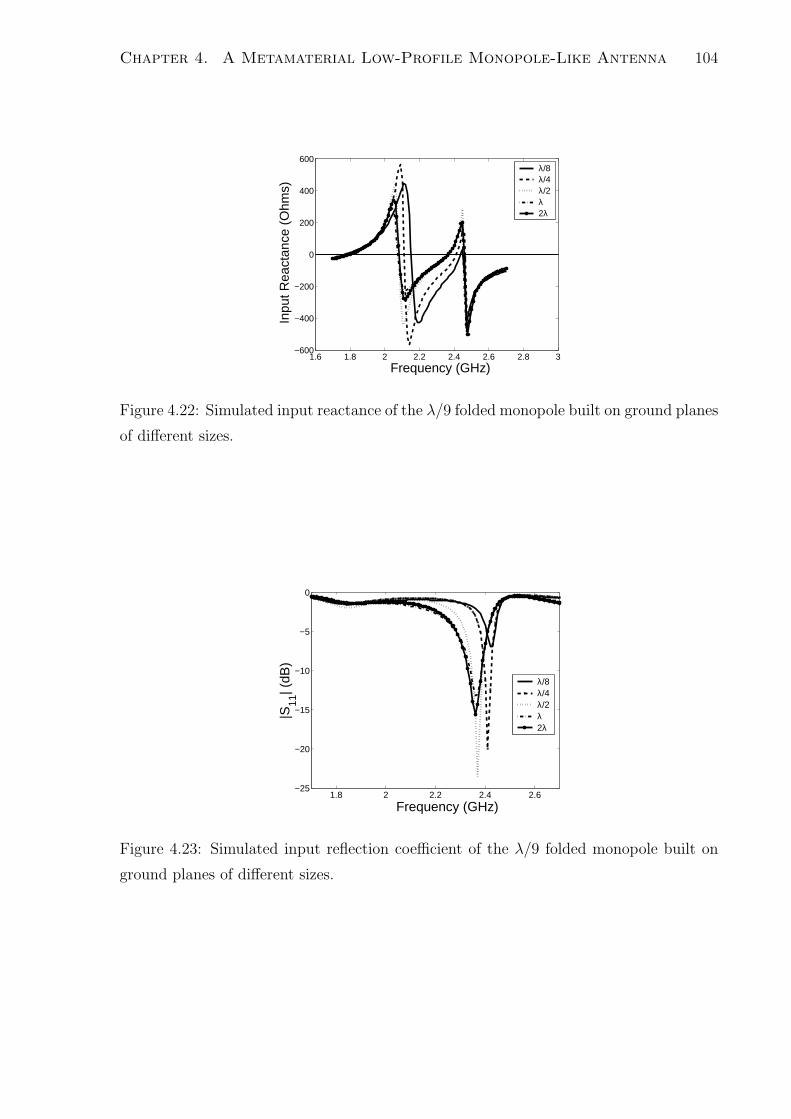
Chapter 4. A Metamaterial Low-Profile Monopole-Like Antenna 104
1.6 1.8 2 2.2 2.4 2.6 2.8 3−600
−400
−200
0
200
400
600
Frequency (GHz)
Inpu
t Rea
ctan
ce (
Ohm
s)
λ/8λ/4λ/2λ2λ
Figure 4.22: Simulated input reactance of the λ/9 folded monopole built on ground planes
of different sizes.
1.8 2 2.2 2.4 2.6−25
−20
−15
−10
−5
0
Frequency (GHz)
|S11
| (dB
)
λ/8λ/4λ/2λ2λ
Figure 4.23: Simulated input reflection coefficient of the λ/9 folded monopole built on
ground planes of different sizes.

Chapter 4. A Metamaterial Low-Profile Monopole-Like Antenna 105
Figure 4.24: Photograph of the proposed λ/9 folded monopole built on a λ/2 × λ/2
ground plane.
4.7.2 Antenna Designs on a λ/2 × λ/2 Ground Plane
Based on the conclusion of the study on the impact of the ground plane size to the input
impedance of the proposed antenna, the fabrication and measurement of two antenna
designs built on a λ/2 × λ/2 ground plane is reported in this section.
λ/9 folded-monopole on a λ/2 × λ/2 ground plane
The first of the two antennas reported in this section is a λ/9 folded-monopole built on
a λ/2 × λ/2 ground plane. Other than the ground plane size, the antenna parameters
are identical with those of the antenna reported in section 4.5. Besides, a sleeve balun
has been used to coaxially feed the antenna and ensure that the feeding cable in not
radiating. A photograph of the fabricated prototype is depicted in Fig. 4.24.
The simulated and measured return losses of this antenna design are shown in Fig.
4.25. A 2.5% −10 dB and a 4% −6 dB fractional bandwidths were measured for this
design. These bandwidths are smaller (approximately by a factor of 2) than those mea-
sured for the antenna fed against the 2λ× 2λ large ground plane. As far as the radiation
patterns are concerned, the simulated and measured E− and H−plane patterns of an-

Chapter 4. A Metamaterial Low-Profile Monopole-Like Antenna 106
1.8 2 2.2 2.4 2.6−30
−25
−20
−15
−10
−5
0
Frequency (GHz)
|S11
| (dB
) MeasuredSimulated
Figure 4.25: Measured and simulated return loss of the λ/9 folded monopole built on a
λ/2 × λ/2 ground plane.
tenna are shown in Fig. 4.26 and Fig. 4.27, respectively. It is noted that the measured
E−plane pattern is not tilted off the θ = 90o direction, as was for the antenna built
on the large ground plane, and is similar to the doughnut-shaped radiation patterns of
conventional dipoles, with the exception of the relatively high cross-polarization levels
that have been measured in the θ = 0o and θ = 180o directions and are attributed to
the radiation of the edges of ground plane. Also, the measured H−plane for this design
is almost perfectly omnidirectional, as opposed to the antenna of section 4.5 where the
standing currents on the corners of the large ground plane affected the H−plane pat-
tern. Radiation efficiencies of the order of 85% were measured for this antenna using the
Directivity/Gain comparison method. Specifically, by measuring the full 3-D radiation
patterns with an angular step of 5o in both the θ− and φ−planes, a maximum direc-
tivity of 2.57 dBi and a maximum gain of 2 dBi were measured at the resonance of the
antenna, yielding an efficiency value of 87.7%. This value is of the same order with the
efficiency values measured using the Wheeler cap method for the antenna built on the
2λ × 2λ large ground plane. Similarly with that antenna, the measured efficiency values
decreased towards the upper edge of the operating band.
λ/17 folded-monopole on a λ/2 × λ/2 ground plane
The second low-profile antenna built and measured on a λ/2 × λ/2 ground plane was a
λ/17 folded-monopole. For this antenna, the thickness of the air layer between the two

Chapter 4. A Metamaterial Low-Profile Monopole-Like Antenna 107
0°
30°
60°
90°
120°
150°
±180°
−150°
−120°
−90°
−60°
−30°
−30
−20
−10
0
Meas. EθSim. EθMeas. EφSim. Eφ
Figure 4.26: Measured and simulated
E−plane radiation pattern of the λ/9
folded monopole built on a λ/2 × λ/2
ground plane.
0°
30°
60°
90°
120°
150°
180°
210°
240°
270°
300°
330°
−30−20
−100
Meas. EθSim. EθMeas. EφSim. Eφ
Figure 4.27: Measured and simulated
H−plane radiation pattern of the λ/9
folded monopole built on a λ/2 × λ/2
ground plane.
dielectric layers has been set to 2.4 mm. According to the conclusions of section 4.6,
further reducing the distance of the spiral-based lines from the ground plane affects the
properties of the phase-shifting lines. Therefore, the λ/17 folded-monopole is among the
very ultra low-profile antenna designs that can be obtained using the proposed approach.
A photograph of the fabricated prototype is shown in Fig. 4.28
The simulated and measured return losses of this antenna are shown in Fig. 4.29.
These results suggest that the λ/17 antenna design does not exhibit satisfying input
resistance to be well-matched to a 50Ω feeding line. In fact, equation (4.3) suggests that
the theoretically estimated radiation resistance for this profile is only 22Ω. Nevertheless,
a measured −8 dB return loss is achieved at 2.45GHz. For this frequency, the simulated
and measured E− and H−plane radiation patterns are shown in Fig. 4.30 and Fig. 4.31,
respectively. These radiation patterns show that even for such low profiles the monopole-
like radiation pattern characteristics are well-retained. Nevertheless, a total radiation
efficiency of only 20% was measured (using the full 3-D radiation pattern measurements
and the Directivity/Gain comparison method) for this antenna.

Chapter 4. A Metamaterial Low-Profile Monopole-Like Antenna 108
a) b)
Figure 4.28: a) Top view and b) side view photograph of the λ/17 low-profile folded
monopole built on a λ/2 × λ/2 ground plane.
1.8 2 2.2 2.4 2.6−14
−12
−10
−8
−6
−4
−2
0
Frequency (GHz)
|S11
| (dB
)
MeasuredSimulated
Figure 4.29: Measured and simulated return loss of the λ/17 folded monopole built on a
λ/2 × λ/2 ground plane.

Chapter 4. A Metamaterial Low-Profile Monopole-Like Antenna 109
−35
−25
15
−5
5
60o
−120o
30o
−150o
0o
270
−30o
150o
−60o
120o
−90o 90o
E−plane (xz−plane)
Sim. Eθ
Sim. Eφ
Meas. Eθ
Meas. Eφ
Figure 4.30: Measured and simulated
E−plane radiation pattern of the λ/17
folded monopole built on a λ/2 × λ/2
ground plane.
−40
−30
−20
−10
0
30o
210o
60o
230o
90o
270o
120o
300o
150o
330o
180o 0o
H−plane (xy−plane)
Sim. Eθ
Sim. Eφ
Meas. Eθ
Meas. Eφ
Figure 4.31: Measured and simulated
H−plane radiation pattern of the λ/17
folded monopole built on a λ/2 × λ/2
ground plane.
4.8 Microstrip-fed Low-Profile Folded Monopoles
Up to this point, all the considered low-profile monopoles were coaxially-fed. In many
applications, though, the use of microstrip feeding lines may drastically simplify the
design and fabrication of the RF front-end. For this reason, the proposed antenna is
tested in this section when considered to be fed by a microstrip line.
The schematic of the proposed microstrip-fed low-profile folded monopole is depicted
in Fig. 4.32. In fact, the only difference between this antenna and the coaxially-fed
monopole is that instead of the antenna to be fed below its ground plane, it is fed from
above the ground plane, using a 50Ω microstrip line. This slightly reduces the total length
of the radiating posts, resulting in a slightly reduced radiation resistance, as compared
to its coaxially-fed counterpart of the same profile. This feature could be inverted by
designing the feeding line at the other side of the ground plane.
The microstrip-fed low-profile monopole of Fig. 4.32 was built similarly as before.
The dielectric material used was again the TACONIC TLY − 5A (ǫr = 2.2). This time
the thickness of the substrates was hsub1 = hsub2 = 1.15 mm, while the ground plane size

Chapter 4. A Metamaterial Low-Profile Monopole-Like Antenna 110
Figure 4.32: a) Top view and b) side view schematic of the microstrip-fed low-profile
antenna.
is set to be λ/2 × λ/2. A photograph of a λ/12 microstrip-fed low-profile monopole is
shown in Fig. 4.33.
Figure 4.33: a) Side view and b)top view photograph of the microstrip-fed low-profile
antenna.
The measured and simulated return losses of the antenna of the λ/12 folded monopole
of Fig. 4.33 are depicted in Fig. 4.34. The simulated results were obtained using CST

Chapter 4. A Metamaterial Low-Profile Monopole-Like Antenna 111
2 2.2 2.4 2.6 2.8 3−20
−18
−16
−14
−12
−10
−8
−6
−4
−2
0
Frequency (GHz)
|S(1
,1)|
(dB
)SimulatedMeasured
Figure 4.34: Simulated and measured return loss of the microstip-fed single element.
Microstripes. As it can be seen in Fig. 4.34, there is a discrepancy between the simulated
and measured results. This can be attributed to two reasons. The first is related to the
full-wave simulation of the structure. In particular, the full-wave simulation of the an-
tenna structure together with the feeding line requires a significantly large computational
domain that could be hardly solved by the available in the lab computational systems.
Therefore, the meshing procedure for this structure was carried out manually, enforcing a
less dense mesh. Also, the convergence criteria employed during the solution of the model
were not so strict. The second reason that might have caused the observed discrepancy
is the fabrication of the antenna and, specifically the microstrip-to-wire transition. It has
been experimentally validated that the quantity of soldering material used to solder the
radiating wire on the microstrip-line influences the inductance of the wire and, therefore,
slightly detunes the final structure.
A second comment on the simulated and measured return losses of the proposed
microstrip-fed low-profile monopole is that even though at resonance the antenna can be
considered matched (|S11| < −10 dB), the return loss does not achieve very small values.
This is attributed to the reduced radiation resistance of the microstrip-fed antenna (as
compared to the coaxially-fed counterpart of the same profile).
The measured E−plane and H−plane radiation patterns of the microstrip-fed an-
tenna are shown in Fig. 4.35 and Fig. 4.36, respectively. These results consist the major
difference between the microstrip-fed and the coaxially-fed antenna. Specifically, given
that in the microstrip-fed case the port is located within one of the two principal planes
of the antenna (H−plane), it significantly affects its radiation patterns resulting in a

Chapter 4. A Metamaterial Low-Profile Monopole-Like Antenna 112
more directive H−plane pattern than the almost perfectly omnidirectional H−plane of
the coaxially-fed antenna. Referring to the H−plane pattern of Fig. 4.36, the feeding
port is located at direction ϕ = 270o and causes the two nulls at the ϕ = 225o and
ϕ = 315o directions. The measured maximum directivity of the microstrip-fed antenna
is 3.16 dBi. The efficiency value that was extracted from the Gain/Comparison method
for the microstrip-fed λ/12 antenna was 43%.
−20
−10
0
0°
30°
60°
90°
120°
150°
±180°
−150°
−120°
−90°
−60°
−30°
EθEφ
Figure 4.35: E-plane radiation pattern
for a single low-profile folded monopole
fed with a microstrip line.
−20
−10
0
0°
30°
60°
90°
120°
150°
180°
210°
240°
270°
300°
330°
EθEφ
Figure 4.36: H-plane radiation pattern
for a single low-profile folded monopole
fed with a microstrip line.
4.9 Coupling Assessment Between Low-Profile Folded
Monopoles
Throughout the study of the proposed low-profile folded monopoles, it has been dis-
covered that one of their major advantages, as compared to conventional monopoles, is
that they exhibit reduced mutual coupling when operating in close proximity to each
other. This feature might be extremely useful for many applications. For this reason,
in this section the coupling between two λ/12 low-profile folded monopoles is assessed
as a function of the distance between them, and compared to the coupling between the
conventional λ/4 monopoles. The assessment is performed through both full-wave and

Chapter 4. A Metamaterial Low-Profile Monopole-Like Antenna 113
2 2.2 2.4 2.6 2.8 3−20
−15
−10
−5
0
Frequency (GHz)
S−
para
met
ers
(dB
)
S11,LPFM
S11,mono
S21,LPFM
S21,mono
Figure 4.37: Return loss and coupling coefficient between two λ/4 monopoles and two
low-profile folded monopoles (LPFM), respectively, being 0.2λ apart.
semi-analytical methods.
4.9.1 Full-wave Analysis
The most accurate assessment of the coupling between any pair of antennas can be
performed through full-wave simulations. In this section, the results of the full-wave
analysis of two-element arrays of conventional monopoles and the proposed low-profile
monopoles are reported.
Inter-element spacing : 0.2λ
In the first case, the inter-element distance is assumed to be d = 25mm or, approximately,
d = 0.2λ. In this case, the return loss and the coupling coefficient between the λ/4
monopoles and the proposed low-profile monopoles are shown in Fig. 4.37. According to
this figure, the maximum coupling level for the low-profile folded monopole is of the order
of S21 = −13.5dB, while for the conventional monopoles the corresponding coupling level
is approximately 3.5 dB larger.
Inter-element spacing : 0.15λ
In the second case, the inter-element distance is assumed to be d = 19 mm or, approx-
imately, d = 0.15λ. In this case, the return loss and the coupling coefficient between

Chapter 4. A Metamaterial Low-Profile Monopole-Like Antenna 114
2 2.2 2.4 2.6 2.8 3−20
−15
−10
−5
0
Frequency (GHz)
S−
para
met
ers
(dB
)
S11,LPFM
S11,mono
S21,LPFM
S21,mono
Figure 4.38: Return loss and coupling coefficient between two λ/4 monopoles and two
low-profile folded monopoles (LPFM), respectively, being 0.15λ apart.
the λ/4 monopoles and the proposed low-profile monopoles are shown in Fig. 4.38. Ac-
cording to this figure, the maximum coupling level for the low-profile folded monopole is
of the order of S21 = −10 dB, while for the conventional monopoles the corresponding
coupling level is approximately 3.0 dB larger. In this case, the coupling between the
conventional monopoles is that high that the monopoles are also detuned.
All the results for the full-wave coupling assessment between pairs of λ/4 monopoles
and the proposed low-profile folded monopoles (LPFM) for different inter-element dis-
tances are summarized in Table 4.3.
A/A λ/4 Monopole Proposed LPFM
d = 0.2λ S21 = −9.0 dB S21 = −13.0 dB
d = 0.15λ S21 = −6.5 dB S21 = −10.0 dB
Table 4.3: Coupling coefficients between pairs of λ/4 monopoles and the proposed low-
profile folded monopoles (LPFM) for different inter-element distances.
4.9.2 Analytical Approach
For the rigorous modeling of the coupling between a pair of monopoles, the EMF method,
as presented in [120], for the calculation of the mutual impedance supported between two
side-by-side dipoles could be employed. Nevertheless, some initial comparative quantita-
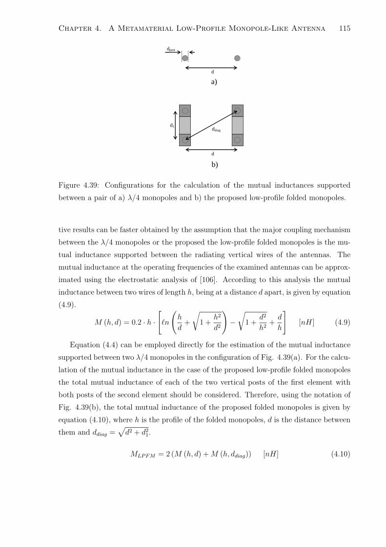
Chapter 4. A Metamaterial Low-Profile Monopole-Like Antenna 115
d
a)
dpost
d
b)
d1 ddiag
Figure 4.39: Configurations for the calculation of the mutual inductances supported
between a pair of a) λ/4 monopoles and b) the proposed low-profile folded monopoles.
tive results can be faster obtained by the assumption that the major coupling mechanism
between the λ/4 monopoles or the proposed the low-profile folded monopoles is the mu-
tual inductance supported between the radiating vertical wires of the antennas. The
mutual inductance at the operating frequencies of the examined antennas can be approx-
imated using the electrostatic analysis of [106]. According to this analysis the mutual
inductance between two wires of length h, being at a distance d apart, is given by equation
(4.9).
M (h, d) = 0.2 · h ·[
ℓn
(
h
d+
√
1 +h2
d2
)
−√
1 +d2
h2+
d
h
]
[nH] (4.9)
Equation (4.4) can be employed directly for the estimation of the mutual inductance
supported between two λ/4 monopoles in the configuration of Fig. 4.39(a). For the calcu-
lation of the mutual inductance in the case of the proposed low-profile folded monopoles
the total mutual inductance of each of the two vertical posts of the first element with
both posts of the second element should be considered. Therefore, using the notation of
Fig. 4.39(b), the total mutual inductance of the proposed folded monopoles is given by
equation (4.10), where h is the profile of the folded monopoles, d is the distance between
them and ddiag =√
d2 + d21.
MLPFM = 2 (M (h, d) + M (h, ddiag)) [nH] (4.10)
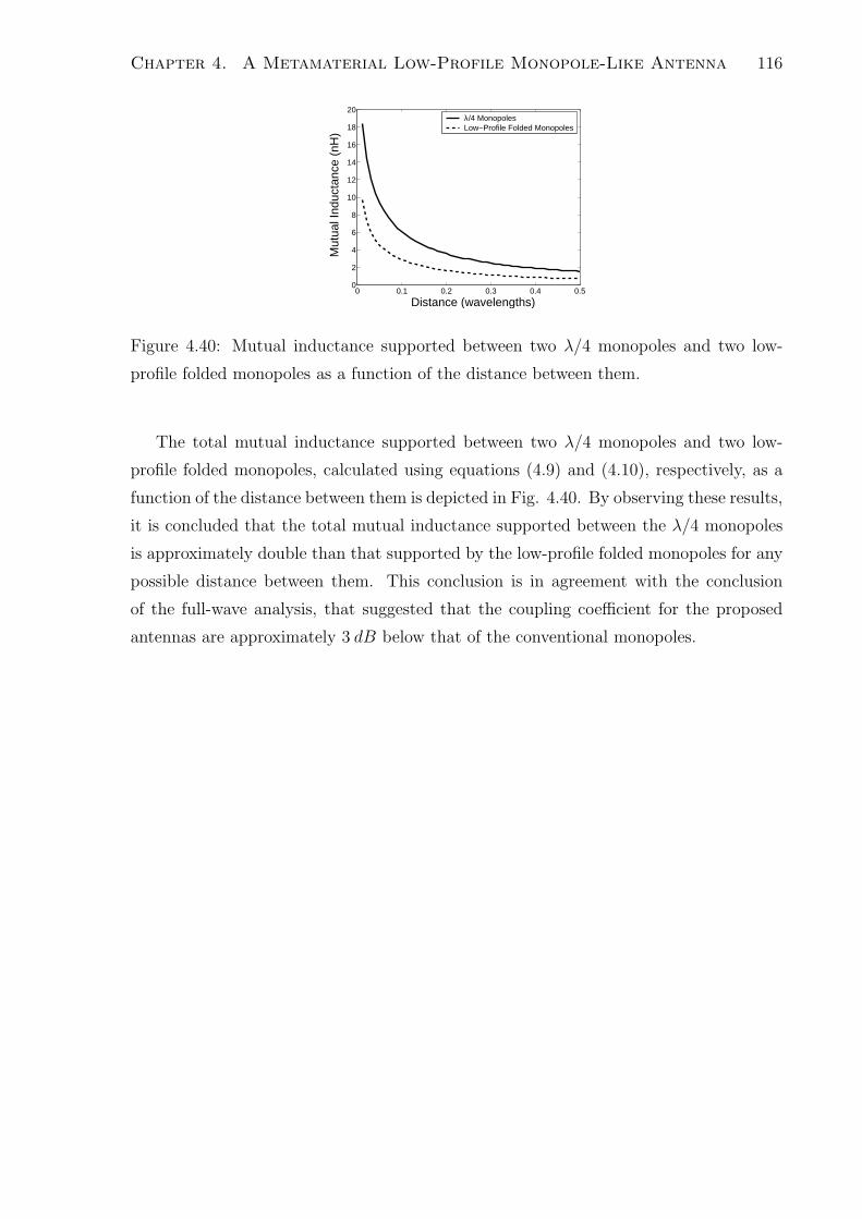
Chapter 4. A Metamaterial Low-Profile Monopole-Like Antenna 116
0 0.1 0.2 0.3 0.4 0.50
2
4
6
8
10
12
14
16
18
20
Distance (wavelengths)
Mut
ual I
nduc
tanc
e (n
H)
λ/4 MonopolesLow−Profile Folded Monopoles
Figure 4.40: Mutual inductance supported between two λ/4 monopoles and two low-
profile folded monopoles as a function of the distance between them.
The total mutual inductance supported between two λ/4 monopoles and two low-
profile folded monopoles, calculated using equations (4.9) and (4.10), respectively, as a
function of the distance between them is depicted in Fig. 4.40. By observing these results,
it is concluded that the total mutual inductance supported between the λ/4 monopoles
is approximately double than that supported by the low-profile folded monopoles for any
possible distance between them. This conclusion is in agreement with the conclusion
of the full-wave analysis, that suggested that the coupling coefficient for the proposed
antennas are approximately 3 dB below that of the conventional monopoles.

Chapter 5
Sub-wavelength Antenna Arrays
In this chapter, three different classes of compact (sub-wavelength) antenna arrays are
designed and investigated. In all of the three cases, emphasis has be given on the en-
hancement of the array performance by means of reducing the electromagnetic coupling
between the individual radiators. The first of these arrays is a two-element phased array
with inter-element separation of the order of 0.2λ. The low-profile folded monopoles pro-
posed in chapter 4 are employed in order to prevent the array performance degradation
caused by the coupling between the array elements. The second investigated class of
sub-wavelength arrays is the superdirective endfire arrays formed by low-profile folded
monopoles. The reduced electromagnetic coupling between these antennas allows for the
design of such arrays without the use of complicated decoupling networks or other tun-
ing elements. Three superdirective arrays are designed and compared in terms of their
achieved directivities and the delivered radiation efficiencies. Finally, a novel approach
for the decoupling of conventional planar inverted-F antennas (PIFAs) built on a com-
mon compact ground plane is presented. The proposed approach could be used for the
implementation of diversity gain schemes in handheld devices.
5.1 Introduction
The use of sub-wavelength antenna arrays in modern communication systems is becoming
more and more frequent. This trend is imposed by the need for miniaturization of mobile
terminals and the implementation of advanced communication techniques that exploit
multiple antenna terminals for more efficient spectral usage (e.g. MIMO, beamforming,
diversity schemes etc). The major difficulty in the design of such sub-wavelength antenna
117

Chapter 5. Sub-wavelength Antenna Arrays 118
arrays is the electromagnetic coupling between the individual radiators that results in the
change of the antennas’ input impedance (increase of the corresponding return loss) and
also the increase of their mutual impedance (increased correlation between the received
signals by different antennas).
In order to overcome these difficulties, two major strategies have be proposed in the
literature. The first of them relies on the use of decoupling feeding networks that com-
pensate for any perturbation of the input impedance of each radiator due to its mutual
impedances with its adjacent radiators [121], [122],[123], [124]. The major disadvantages
of this approach are that for the efficient design of the decoupling networks the mutual
impedances of the array elements should be known a priori (a condition that can not be
always satisfied) and that imperfections in the operation of the decoupling networks (e.g.
ohmic losses) degrade the performance of the designed arrays.
The second approach for the reduction of the coupling between radiators partici-
pating in arrays is the use of insulating structures between the radiating elements [72],
[125], [126]. This approach became quite popular with the advent of electromagnetic
bandgap (EBG) and other metamaterial structures that can act as electromagnetic in-
sulators between the radiating elements. The major disadvantage of this approach is
that the employed insulating structures are being placed in the near-field of the radiat-
ing elements, affecting the radiating properties of the antennas and dissipating power.
Besides, given that the insulating structures are usually periodic structures, they occupy
certain volume/area and therefore their use in ultra compact arrays encounters practical
restrictions.
In this chapter, it is shown that sub-wavelength arrays could be designed and effec-
tively operate without the use of decoupling networks or insulating structures, provided
that self-resonant radiating elements exhibiting ultra low coupling between them are be-
ing employed. The low-profile folded monopoles of chapter 4 meet all these requirements
and, hence, in this chapter are employed for the design of sub-wavelength arrays. Specif-
ically, first, a two-element sub-wavelength phased array, composed of two low-profile
folded monopoles and designed to scan its beam at 60o off broadside, is built and com-
pared with the corresponding sub-wavelength array that is composed of λ/4 monopoles.
In turn, the theory for the design of superdirective endfire arrays, that considers uncou-
pled array elements, along with the proposed low-profile folded monopoles, are effectively
employed for the synthesis of sub-wavelength superdirective endfire arrays. Finally, for
applications that require the use of arrays of conventional antennas, such as PIFAs, built

Chapter 5. Sub-wavelength Antenna Arrays 119
within small volumes, a simplified metamaterial-inspired approach is proposed for the
decoupling of such antenna elements.
5.2 Sub-wavelength Phased Arrays
In this section of the chapter a sub-wavelength two-element phased array comprising of
low-profile folded monopoles is built and its performance is compared to a two-element
phased array composed of conventional λ/4 monopoles. The purpose of this study is
to examine the potential advantages of sub-wavelength arrays composed of low-coupling
radiating elements as compared to their conventional counterparts.
The design procedure starts with the assumption of the design parameters of the
phased array. First, the targeted operating frequency of the sub-wavelength phased
array is set to be 2.45 GHz. For the design of the considered sub-wavelength phased
array, microstrip technology will be employed. In this framework, both the low-profile
folded monopoles and the feeding network will be microstrip-based. This will enable
the simplification of the fabrication procedure, reduce the fabrication cost (fully-printed
feeding network and radiating elements) and will also allow the direct deployment of the
array (passive, single-port-fed antenna).
The fully-printed, microstrip-based feeding network that will be employed for the
design of the sub-wavelength phased array is depicted in Fig. 5.1. It is composed of a
quadrature hybrid that equally splits the power of a single microstrip feeding port and
provides two signals of equal amplitude being −90o out-of-phase. Then, a transmission
line segment of electrical length −215o connected in series with the out-of-phase port
secures a 55o phase difference between the two output ports at 2.45 GHz. The physical
distance between these ports is d = 22.0mm. Given that this feeding network was already
available when the sub-wavelength phased arrays were investigated, it was decided for the
built phased array to be fed with a phase progression of a = 55o and the array elements
to be at a distance d = 22.0 mm. At 2.45 GHz, this physical length corresponds to an
electrical length of βd = 0.36π. The normalized array factor of the two-element array is
then given by equation (5.1), where φ = ±90o along the axis of the array, and φ = 0o in
the broadside direction.
|AF (φ)| =
∣
∣
∣
∣
cos
(
βdsinφ + a
2
)∣
∣
∣
∣
(5.1)

Chapter 5. Sub-wavelength Antenna Arrays 120
Equation (5.1) assumes its maximum when∣
∣cos(
βdsinφ+a
2
)∣
∣ = 1, or equivalently when
βdsinφ + a = 0. For a phase progression a = 55o, an ideal two-element array similar
with the one under investigation is expected to scan its beam at 58o off broadside.
Figure 5.1: Microstrip-based feeding network employed for the synthesis of the two-
element sub-wavelength phased array.
The feeding network of Fig. 5.1 was built on 1.15 mm thick TACONIC TLY − 5A
dielectric substrate (ǫr = 2.2). The simulated (ANSOFT Designer) S−parameters of the
feeding network are shown in Fig. 5.2 and Fig. 5.3 (magnitude and phase, respectively).
These results validate that the quadrature hybrid is designed to operate in the 2.45GHz
band. Specifically, at 2.45 GHz |S11| < −20 dB, |S21| ≈ |S31| ≈ −3 dB and also ∠S31 −∠S21 ≈ 55o.
The feeding network of Fig. 5.1 is employed to feed two different two-element antenna
arrays. In the first array, the radiating elements are low-profile folded monopoles, iden-
tical with those presented in section 4.8. Their profile is considered to be h = 10.3 mm
(λ/12). In the second array, the radiating elements are conventional λ/4 monopoles.
Both types of monopoles are directly attached at the open ends of the feeding networks.
A photograph of the fabricated array with the low-profile folded monopoles is depicted
in Fig. 5.4.
In the following text, the two phased arrays are compared in terms of their measured
performance. Specifically, in Fig. 5.5 the return losses of the two arrays are shown. As
expected, the return loss of the conventional monopoles are much more broadband than
the return loss of the low-profile folded monopoles array. Nevertheless, both arrays can
be considered to be matched at 2.45 GHz (|S11 < −10 dB|).

Chapter 5. Sub-wavelength Antenna Arrays 121
2 2.2 2.4 2.6 2.8 3−30
−25
−20
−15
−10
−5
0
Frequency (GHz)
S−
para
met
ers
(dB
)
|S11
||S
31|
|S21
|
Figure 5.2: S−parameters (magnitude) of the feeding network of Fig. 5.1.
2 2.2 2.4 2.6 2.8 3−200
−150
−100
−50
0
50
100
150
200
Frequency (GHz)
Pha
se (
Deg
rees
)
Arg(S21
)Arg(S
31)
Figure 5.3: S−parameters (phase) of the feeding network of Fig. 5.1.
In Fig. 5.6 the normalized patterns of the two arrays under investigation are plot-
ted. The range of the patterns extends from −90o to +90o. These results show that the
radiation pattern of the low-profile monopole array achieves its maximum closer to the
theoretically calculated scanning angle of ϕo = 58o. Specifically, the low-profile monopole
array scans its beam at 55o while the conventional monopole array scans its beam at 50o.
It is noted that the angular resolution during the radiation pattern measurements is
5o. One potential physical explanation for the divergence between the measured and
the theoretically calculated scanning angles could be the coupling between the radiating
elements of the array, that affects the feeding phase of each of the elements of the array.

Chapter 5. Sub-wavelength Antenna Arrays 122
Figure 5.4: Photograph of the fabricated prototype of the investigated sub-wavelength
phased array of low-profile folded monopoles.
2400 2420 2440 2460 2480 2500−18
−16
−14
−12
−10
−8
−6
−4
−2
Frequency (GHz)
|S11
| (dB
)
LPFMλ/4 Monopoles
Figure 5.5: Measured return losses (S11) of the two sub-wavelength arrays.
In that case, given that the coupling between the low-profile folded monopoles has been
shown to be weaker than that between conventional monopoles, the performance of the
low-profile array is less affected by the coupling and the error in its scanning angle be-
comes smaller. Finally, the measured results show that the delivered radiation efficiency
of the low-profile array (this efficiency was measured to be 45%) is almost equal with
that of the conventional array (the radiation efficiency for the conventional array was
measured to be 48%). Even though this result is slightly counterintuitive, given that the
low-profile monopoles are significantly less efficient than conventional monopoles, this
result was validated through multiple measurements.
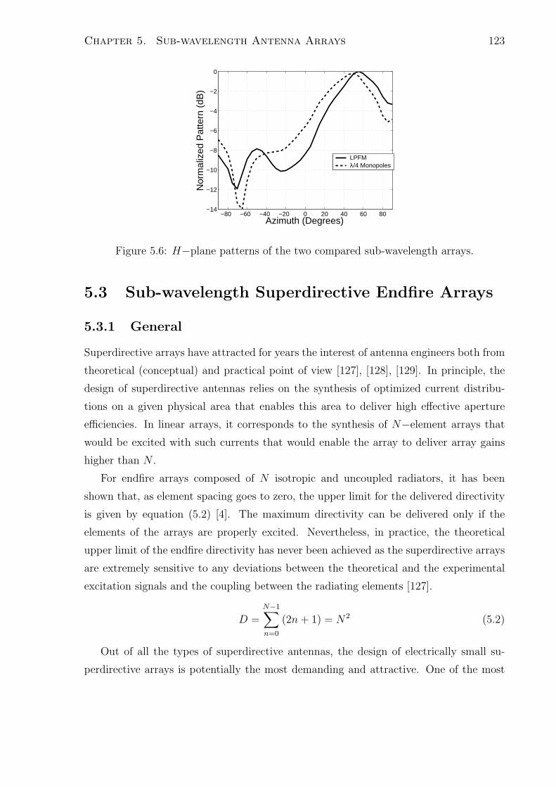
Chapter 5. Sub-wavelength Antenna Arrays 123
−80 −60 −40 −20 0 20 40 60 80−14
−12
−10
−8
−6
−4
−2
0
Azimuth (Degrees)
Nor
mal
ized
Pat
tern
(dB
)
LPFMλ/4 Monopoles
Figure 5.6: H−plane patterns of the two compared sub-wavelength arrays.
5.3 Sub-wavelength Superdirective Endfire Arrays
5.3.1 General
Superdirective arrays have attracted for years the interest of antenna engineers both from
theoretical (conceptual) and practical point of view [127], [128], [129]. In principle, the
design of superdirective antennas relies on the synthesis of optimized current distribu-
tions on a given physical area that enables this area to deliver high effective aperture
efficiencies. In linear arrays, it corresponds to the synthesis of N−element arrays that
would be excited with such currents that would enable the array to deliver array gains
higher than N .
For endfire arrays composed of N isotropic and uncoupled radiators, it has been
shown that, as element spacing goes to zero, the upper limit for the delivered directivity
is given by equation (5.2) [4]. The maximum directivity can be delivered only if the
elements of the arrays are properly excited. Nevertheless, in practice, the theoretical
upper limit of the endfire directivity has never been achieved as the superdirective arrays
are extremely sensitive to any deviations between the theoretical and the experimental
excitation signals and the coupling between the radiating elements [127].
D =N−1∑
n=0
(2n + 1) = N2 (5.2)
Out of all the types of superdirective antennas, the design of electrically small su-
perdirective arrays is potentially the most demanding and attractive. One of the most

Chapter 5. Sub-wavelength Antenna Arrays 124
challenging tasks in the design of a superdirective electrically small array is the design of
its feeding network. Such a feeding network usually performs two majors tasks. First, it
is responsible for the matching of the electrically small radiating elements that, in most
cases, are not self-resonant. Secondly, it decouples the radiating elements that, being in
close proximity, exhibit high mutual impedances and properly sets the relative magni-
tude and phase of the excitation signals at the port of each antenna of the array. The
complexity of these networks and the imperfections associated with their operation (i.e.
ohmic losses) are usually the reasons for not experimentally demonstrating the maximum
directivity of equation (5.2).
With the use of metamaterial structures some of the issues currently handled by the
feeding network could be possibly addressed in a different way, simplifying the design
of the feeding network and improving its performance. For example, in [72], the use
of a metamaterial insulator was proposed for the decoupling of the array elements. In
the present work, the self-resonant low-profile folded monopoles presented in chapter 4,
that exhibit reduced mutual coupling, are employed for the design of two-element endfire
superdirective arrays. Given the features of the employed radiators (self-resonant, low-
coupling), the feeding network can be simplified and perform a single function; that of
properly setting the excitation currents of the array elements. As a result, this feeding
network becomes simple to design, low-cost and easy to fabricate.
5.3.2 Feeding Network
As it has been already mentioned, in this approach, self-resonant, low-coupling radiating
elements are employed for the design of two-element superdirective endfire arrays. As
a result, the required feeding network implements a single function, that of setting the
proper excitation currents at the inputs of the two radiating elements. Based on the
analysis of [4], for two-element arrays, endfire superdirective patterns are obtained when
the two radiators are fed with currents equal in magnitude and a relative phase-shift equal
with that of Fig. 5.7. As Fig. 5.7 suggests, the phase-shift between the two elements
is dependent on the distance between them. Therefore different separation between the
radiators would require different phase-shifts to deliver superdirective patterns.
The results of Fig. 5.7 show that the required phase-shift between the excitation
currents of the two radiating elements of the considered superdirective antennas are of
the order of 140o − 180o. Therefore, the required feeding network has been chosen to be

Chapter 5. Sub-wavelength Antenna Arrays 125
0 0.1 0.2 0.3 0.4 0.5140
150
160
170
180
190
200
Spacing (λ)
Rel
ativ
e P
hase
Diff
eren
ce (
degr
ees)
Element 2
Figure 5.7: Relative excitation phase, according to the analysis of [4], for the design of
two-element superdirective arrays.
implemented through a 180o microstrip-based ring hybrid. Specifically, the differential
ports of the hybrid are employed together with transmission line segments of proper
length connected in series to them to synthesise the required pairs of phase-shift and
distance according to Fig. 5.7. The ring-based feeding network is depicted in Fig. 5.8.
The single feeding port of the antenna arrays is considered the port 1 of the ring of Fig.
5.8. The incoming signal is split into two equal in magnitude and 180o out of phase
output signals. The length of the transmission line segments attached to the output
ports of the hybrid are properly adjusted so that the distance d between the physical
ports 2 and 4 of the feeding network corresponds to the phase required for the synthesis
of the two-element endfire superdirective array (according to the results of Fig. 5.7).
Figure 5.8: Top view schematic of the modified ring hybrid used as feeding network for
the proposed superdirective endfire two-element array designs.
The feeding network of Fig. 5.8 is built on a TACONIC TLY − 5A dielectric

Chapter 5. Sub-wavelength Antenna Arrays 126
substrate of dielectric constant ǫr = 2.2 and is designed for operation in the 2.45 GHz
band. The S−parameters of this feeding network, optimized to feed a superdirective
endfire array with element separation of 0.2λ, are shown in Fig. 5.9.
2 2.2 2.4 2.6 2.8 3−8
−6
−4
−2
0
|S|(d
B)
Frequency (GHz)2 2.2 2.4 2.6 2.8 3
−200
−100
0
100
200
phas
e di
ffere
nce
(ºde
g)
Frequency (GHz)
|S(2,1)||S(4,1)|ang(S(4,2))
Figure 5.9: Insertion loss and phase difference between the two output ports of the
modified hybrid of Fig. 5.8.
5.3.3 Driven Superdirective Arrays
In the following text, the measurement results of two different designs of superdirective
enfdire arrays driven by the feeding network of Fig. 5.8 are presented. A representative
schematic of the fabricated and measured driven superdirective arrays is shown in Fig.
5.10.
In the first of the fabricated prototypes, the separation between the radiating elements
is considered to be 0.2λ. The employed feeding network and its S−parameters are those
presented in the previous section. In the second fabricated prototype, the separation
between the radiating elements is decreased to 0.15λ. For this design the transmission
line segments attached to the outputs of the ring have been adjusted according to the
requirements suggested by Fig. 5.7. It is noted that for both these designs the height of
the employed low-profile monopoles is h = 10.3 mm (λ/12)

Chapter 5. Sub-wavelength Antenna Arrays 127
Figure 5.10: A schematic representation of the proposed superdirective arrays.
0.2λ Array
The first fabricated prototype is the 0.2λ array. A photograph of this prototype is shown
in Fig. 5.11.
Figure 5.11: Photograph of the fabricated two-element superdirective endfire array.
The measured and simulated return loss of the prototype of Fig. 5.11 is depicted in

Chapter 5. Sub-wavelength Antenna Arrays 128
Fig. 5.12. These results show that the designed array is matched at the target frequency
of 2.45 GHz. The second deep that appears at the return loss curve at approximately
2.1GHz, and is more profound for the simulated results, corresponds to the transmission
line resonance of the employed low-profile folded monopoles.
2 2.2 2.4 2.6 2.8 3−30
−25
−20
−15
−10
−5
0
Frequency (GHz)
|S(1
,1)|
(dB
)
SimulatedMeasured
Figure 5.12: Return loss for the 0.2λ superdirective endfire array.
To experimentally show the highly directive properties of the fabricated prototype,
the radiation patterns of the array were measured and compared to that of a single
microstrip-fed low-profile folded monopole. As was expected, the directive properties
of the synthesised arrays appear in the H-plane. The measured H-plane of the 0.2λ
prototype, measured at 2.45 GHz, together with that of the single low-profile monopole,
are depicted in Fig. 5.13.
These results suggest that the synthesised array exhibits a much more directive pat-
tern than the single element. Specifically, the directivity of the array in the endfire
direction was measured to be 5.7dBi, while the directivity of the single low-profile folded
monopole in the same direction had been measured to be 3.17 dBi.
0.15λ Array
The 5.7 dBi of the 0.2λ array do not prove the superdirective properties of the designed
array, given that the two-element array exhibits less than 3dB improvement in the direc-
tivity as compared to the single element. A second attempt to implement a superdirective,
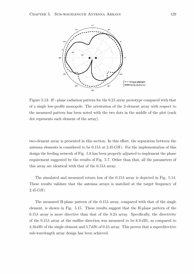
Chapter 5. Sub-wavelength Antenna Arrays 129
Figure 5.13: H−plane radiation pattern for the 0.2λ array prototype compared with that
of a single low-profile monopole. The orientation of the 2-element array with respect to
the measured pattern has been noted with the two dots in the middle of the plot (each
dot represents each element of the array).
two-element array is presented in this section. In this effort, the separation between the
antenna elements is considered to be 0.15λ at 2.45 GHz. For the implementation of this
design the feeding network of Fig. 5.8 has been properly adjusted to implement the phase
requirement suggested by the results of Fig. 5.7. Other than that, all the parameters of
this array are identical with that of the 0.15λ array.
The simulated and measured return loss of the 0.15λ array is depicted in Fig. 5.14.
These results validate that the antenna arrays is matched at the target frequency of
2.45 GHz
The measured H-plane pattern of the 0.15λ array, compared with that of the single
element, is shown in Fig. 5.15. These results suggest that the H-plane pattern of the
0.15λ array is more directive than that of the 0.2λ array. Specifically, the directivity
of the 0.15λ array at the endfire direction was measured to be 6.9 dBi, as compared to
3.16dBi of the single element and 5.7dBi of 0.2λ array. This proves that a superdirective
sub-wavelength array design has been achieved.
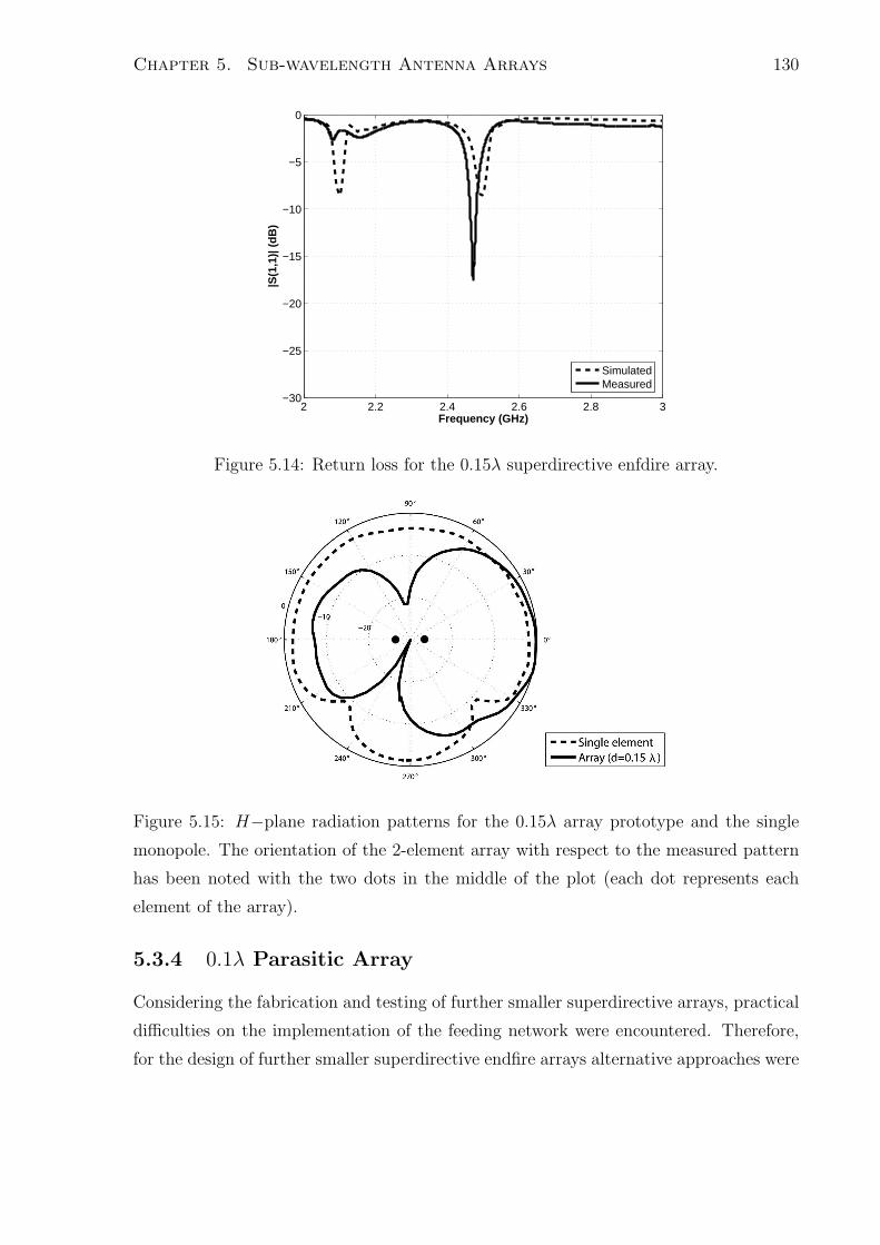
Chapter 5. Sub-wavelength Antenna Arrays 130
2 2.2 2.4 2.6 2.8 3−30
−25
−20
−15
−10
−5
0
Frequency (GHz)
|S(1
,1)|
(dB
)
SimulatedMeasured
Figure 5.14: Return loss for the 0.15λ superdirective enfdire array.
Figure 5.15: H−plane radiation patterns for the 0.15λ array prototype and the single
monopole. The orientation of the 2-element array with respect to the measured pattern
has been noted with the two dots in the middle of the plot (each dot represents each
element of the array).
5.3.4 0.1λ Parasitic Array
Considering the fabrication and testing of further smaller superdirective arrays, practical
difficulties on the implementation of the feeding network were encountered. Therefore,
for the design of further smaller superdirective endfire arrays alternative approaches were

Chapter 5. Sub-wavelength Antenna Arrays 131
searched.
As Fig. 5.7 suggests, for inter-element separations smaller than 0.15λ and as d → 0
the phase-shift between the feeding currents of the two elements moves linearly to 180o.
This observation, together with the fact that for such small separations between the low-
profile monopoles the electromagnetic coupling is not insignificant, lead to the conclusion
that two-element superdirective endfire arrays could be designed with the one of the
elements being directly-fed and the other being parasitically-fed, as also suggested in
[130]. Similarly with the Yagi-Uda antennas, the excited current on the parasitically-fed
element is expected to be approximately equal in magnitude and roughly 180o out of
phase, as compared with the current of the directly-fed element, implementing in that
way the requirement imposed by Fig. 5.7
Based on these arguments, a parasitic two-element array, with element separation
equal to 0.1λ was built and its electromagnetic properties were measured. For the fab-
rication of this array, a ground plane of identical dimensions with those of the driven
arrays was employed. The driven element was fed using a 50 Ω microstrip-line, while
both posts of the parasitic element were shorted to the common ground plane. Given
that a microstrip-fed low-profile folded monopole is slightly electrically smaller than an
identical shorted folded monopole, in the proposed two-element array the parasitic ele-
ment behaves as the reflector of a conventional two-element Yagi-Uda antenna.
The measured and simulated return loss of the parasitic array is depicted in Fig. 5.16
and its H−plane is depicted in Fig. 5.17.
The measured directivity of the parasitic array in the endfire direction was measured
to be 7.6 dBi.
5.3.5 Comparison
All the presented antenna designs exhibited enhanced directivities as compared to the
single low-profile monopole. Specifically, it has been shown that the achieved directivity is
increasing as the distance between the antenna elements is decreasing, as also suggested
by the theory for the design of superdirective arrays. Nevertheless, a more inclusive
characterization and comparison of the three different designs showed that the increment
of the directive properties of the arrays is accompanied by a decrease in their radiation
efficiencies. Specifically, the use of the Directivity/Gain comparison method for the
estimation of the efficiency of each of the designs provided the results presented in Table

Chapter 5. Sub-wavelength Antenna Arrays 132
2 2.2 2.4 2.6 2.8 3−30
−25
−20
−15
−10
−5
0
Frequency (GHz)
|S(1
,1)|
(dB
)
SimulatedMeasured
Figure 5.16: Return loss for the 0.1λ parasitic array.
Figure 5.17: H−plane radiation patterns for the 0.10λ array prototype and the single
monopole. The orientation of the 2-element array with respect to the measured pattern
has been noted with the two dots in the middle of the plot (each dot represents each
element of the array).
5.1. These results show that the most directive array design (parasitic array) achieves an
average efficiency of only 24%, while the directivity of the least directive array (0.2λ) was
measured to be 40%, which is very close with the efficiency of the single element (43%).
This trent is attributed to the fact that decrease of the inter-element separation leads to
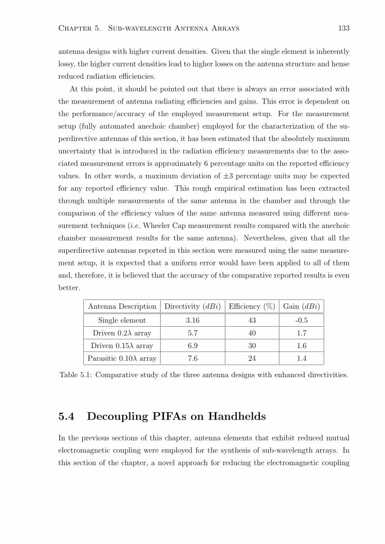
Chapter 5. Sub-wavelength Antenna Arrays 133
antenna designs with higher current densities. Given that the single element is inherently
lossy, the higher current densities lead to higher losses on the antenna structure and hense
reduced radiation efficiencies.
At this point, it should be pointed out that there is always an error associated with
the measurement of antenna radiating efficiencies and gains. This error is dependent on
the performance/accuracy of the employed measurement setup. For the measurement
setup (fully automated anechoic chamber) employed for the characterization of the su-
perdirective antennas of this section, it has been estimated that the absolutely maximum
uncertainty that is introduced in the radiation efficiency measurements due to the asso-
ciated measurement errors is approximately 6 percentage units on the reported efficiency
values. In other words, a maximum deviation of ±3 percentage units may be expected
for any reported efficiency value. This rough empirical estimation has been extracted
through multiple measurements of the same antenna in the chamber and through the
comparison of the efficiency values of the same antenna measured using different mea-
surement techniques (i.e. Wheeler Cap measurement results compared with the anechoic
chamber measurement results for the same antenna). Nevertheless, given that all the
superdirective antennas reported in this section were measured using the same measure-
ment setup, it is expected that a uniform error would have been applied to all of them
and, therefore, it is believed that the accuracy of the comparative reported results is even
better.
Antenna Description Directivity (dBi) Efficiency (%) Gain (dBi)
Single element 3.16 43 -0.5
Driven 0.2λ array 5.7 40 1.7
Driven 0.15λ array 6.9 30 1.6
Parasitic 0.10λ array 7.6 24 1.4
Table 5.1: Comparative study of the three antenna designs with enhanced directivities.
5.4 Decoupling PIFAs on Handhelds
In the previous sections of this chapter, antenna elements that exhibit reduced mutual
electromagnetic coupling were employed for the synthesis of sub-wavelength arrays. In
this section of the chapter, a novel approach for reducing the electromagnetic coupling
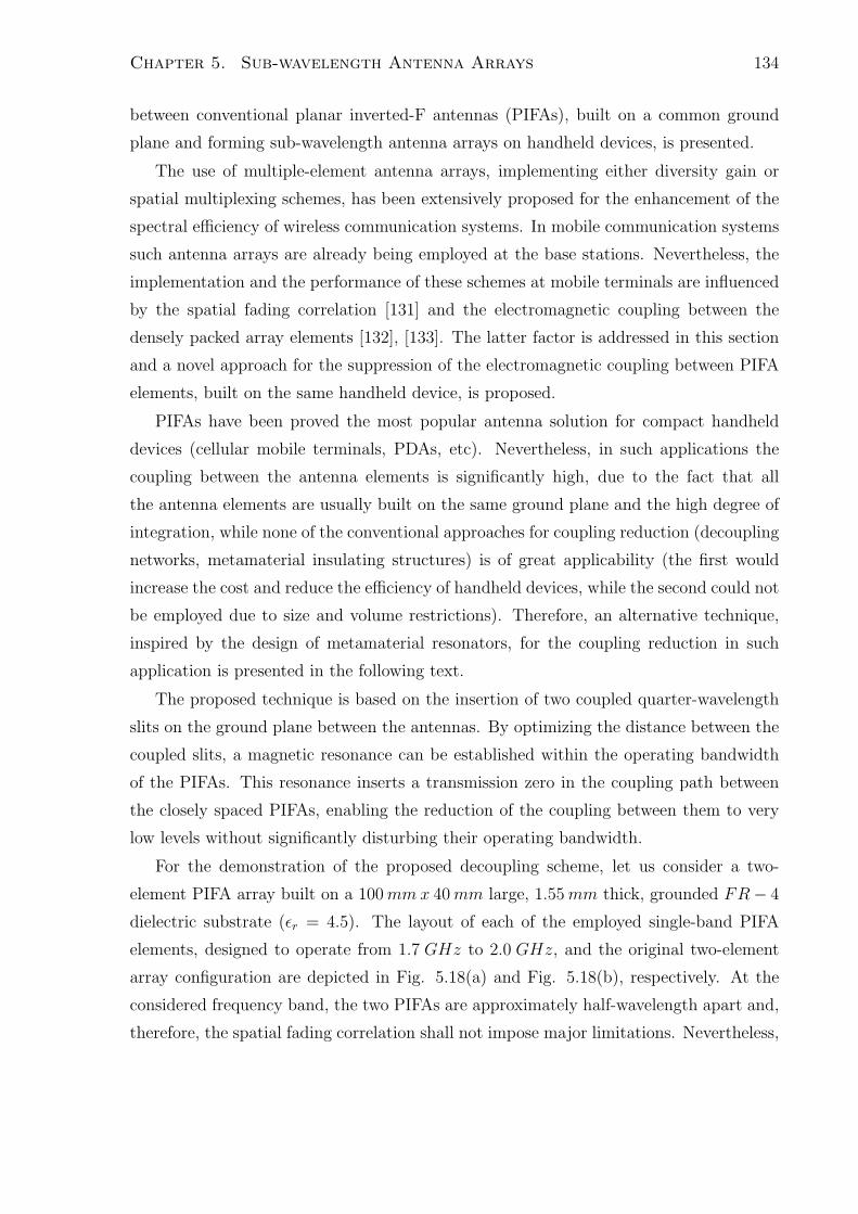
Chapter 5. Sub-wavelength Antenna Arrays 134
between conventional planar inverted-F antennas (PIFAs), built on a common ground
plane and forming sub-wavelength antenna arrays on handheld devices, is presented.
The use of multiple-element antenna arrays, implementing either diversity gain or
spatial multiplexing schemes, has been extensively proposed for the enhancement of the
spectral efficiency of wireless communication systems. In mobile communication systems
such antenna arrays are already being employed at the base stations. Nevertheless, the
implementation and the performance of these schemes at mobile terminals are influenced
by the spatial fading correlation [131] and the electromagnetic coupling between the
densely packed array elements [132], [133]. The latter factor is addressed in this section
and a novel approach for the suppression of the electromagnetic coupling between PIFA
elements, built on the same handheld device, is proposed.
PIFAs have been proved the most popular antenna solution for compact handheld
devices (cellular mobile terminals, PDAs, etc). Nevertheless, in such applications the
coupling between the antenna elements is significantly high, due to the fact that all
the antenna elements are usually built on the same ground plane and the high degree of
integration, while none of the conventional approaches for coupling reduction (decoupling
networks, metamaterial insulating structures) is of great applicability (the first would
increase the cost and reduce the efficiency of handheld devices, while the second could not
be employed due to size and volume restrictions). Therefore, an alternative technique,
inspired by the design of metamaterial resonators, for the coupling reduction in such
application is presented in the following text.
The proposed technique is based on the insertion of two coupled quarter-wavelength
slits on the ground plane between the antennas. By optimizing the distance between the
coupled slits, a magnetic resonance can be established within the operating bandwidth
of the PIFAs. This resonance inserts a transmission zero in the coupling path between
the closely spaced PIFAs, enabling the reduction of the coupling between them to very
low levels without significantly disturbing their operating bandwidth.
For the demonstration of the proposed decoupling scheme, let us consider a two-
element PIFA array built on a 100 mm x 40 mm large, 1.55 mm thick, grounded FR − 4
dielectric substrate (ǫr = 4.5). The layout of each of the employed single-band PIFA
elements, designed to operate from 1.7 GHz to 2.0 GHz, and the original two-element
array configuration are depicted in Fig. 5.18(a) and Fig. 5.18(b), respectively. At the
considered frequency band, the two PIFAs are approximately half-wavelength apart and,
therefore, the spatial fading correlation shall not impose major limitations. Nevertheless,

Chapter 5. Sub-wavelength Antenna Arrays 135
PIFA 1
PIFA 2
d
λ/4
JM
JM
-JM
1
0
0
m
m
40 mm
b) c) d)
Effective
Magnetic
Loop
a)
Figure 5.18: Layout of the a) single PIFA element, b) two-element array on handheld (no
slits on the ground plane), c) coupling reduction scheme by inserting a single slit (notch)
on the ground plane, d) coupling reduction scheme by inserting two coupled slits at a
distance d from each other.

Chapter 5. Sub-wavelength Antenna Arrays 136
the electromagnetic coupling between the two array elements, that is attributed mostly to
the currents on the common ground plane, was found to be relatively high. Specifically,
the structure was simulated using CST Microwave Studio (CST MWS) and the maximum
coupling between the antennas was found to be S21 = −9dB (Fig. 5.19, original design).
A well-known practice in reducing the coupling between antenna elements built on
a common ground plane is the introduction of resonant defects on the ground plane
between the antennas [134], [135]. Such an approach is shown in Fig. 5.18(c), where
a slit (represented also as a magnetic current JM) has been inserted at the edge of the
ground plane. By properly setting the length of the slit to be 29 mm (approximately a
quarter-wavelength at the middle of the operating bandwidth), the slit resonates acting
as a notch and trapping some of the power that was to be transmitted between the
two radiating elements. In fact, for the configuration of Fig. 5.18(c) it was found that
the insertion of such a slit reduces the coupling between the antennas by approximately
4.5 dB (in this case S21 = −13.5 dB, as shown in Fig. 5.19). The coupling between
the two antennas can be further reduced by inserting a second slit of the same length
at a distance d from the first slit, as in Fig. 5.18(d). In the general case, the second
notch introduces another 4.5 dB reduction of the coupling between the antennas (for
the configuration of Fig. 5.18(d), with an arbitrarily chosen value for d, S21 = −18dB).
Nevertheless, even in that case the coupling between the PIFAs, being approximately
half-wavelength apart, remains above -20 dB.
In the proposed approach, it is suggested that a configuration similar with that of Fig.
5.18(d) can be employed to achieve coupling coefficient values significantly below −20dB,
provided that the distance between the two slits is properly chosen. Careful examination
of the electromagnetic fields in the configuration of Fig. 5.18(d) suggests that the two
slits are coupled. Hence, by optimizing the distance between them, they can be made
to resonate forming an effective magnetic loop. By this means, a transmission zero is
introduced in the coupling path between the two radiating elements, reducing further the
electromagnetic coupling between them. Full-wave optimization of the distance between
the slits, carried out using CST MWS, showed that the value of d that makes the coupled
slits to resonate at 1.85GHz (middle frequency of the operating band) is d = 11mm. In
order to show that the distance between the slits can be set so as for the coupled pair of
slits to behave as a magnetic loop, the currents on the ground plane and the electric field
normal to it are depicted in Fig. 5.20. These results validate that the currents on the slits
simultaneously achieve their maximum values (being in phase), resulting in a common,
Chapter 5. Sub-wavelength Antenna Arrays 137
1.2 1.4 1.6 1.8 2 2.2 2.4 2.6 2.8−50
−45
−40
−35
−30
−25
−20
−15
−10
−5
0
Frequency (GHz)
S−
para
met
ers
(dB
)
|S11
| one slit
|S11
| two slits
|S11
| resonating slits
|S11
| original design
|S21
| one slit
|S21
| two slits
|S21
| resonating slits
|S21
| original design
Figure 5.19: Simulated (using CST MWS) S−parameters of the two-element array in the
cases that no slits (original design), one slit, two slits and two resonating coupled slits
have been inserted on the common ground plane.

Chapter 5. Sub-wavelength Antenna Arrays 138
Figure 5.20: Ground plane currents and normal electric field for the resonating effective
magnetic loop.
maximized vertical electric field component in the area between the two coupled slits.
For the value of d that the two slits behave as a resonating magnetic loop, the coupling
between the two antennas is also plotted in Fig. 5.19. This result suggests that for the
resonating coupled slits, the coupling between the PIFAs, at 1.85 GHz, drops below
−50 dB (transmission zero), while it remains below −23 dB for the whole bandwidth of
interest. At this bandwidth both PIFAs remain matched (S11 < −6dB and S22 < −6dB),
even though their input impedances are slightly altered.
It is noted that the resonating coupled slits are expected to radiate. Therefore, the
radiation patterns of the proposed decoupled antenna array have been studied and have
been found to be slightly different than those of the array without the slits. In fact, the
patterns of the proposed structure is slightly more omni-directional (maximum directivity
of 3.5 dBi compared to 4.5 dBi) which is well suited for handset applications. This is

Chapter 5. Sub-wavelength Antenna Arrays 139
Figure 5.21: Radiation patterns comparison between the conventional and the decoupled
PIFA arrays at 1.85 GHz.
shown in Fig. 5.21, where the radiation patterns for the two compared cases have been
plotted. Also, regarding the radiation efficiency of the decoupled array elements, it has
been found that the proposed scheme for the reduction of coupling decreases the efficiency
of each of the radiating elements by approximately 4% (due to the strong currents on
the ground plane).
In order to experimentally validate the proposed technique for coupling reduction
between PIFAs built on the same ground plane, two antenna prototypes (the original
array and the one with the resonating coupled slits) have been fabricated and measured.
The measured S−parameters in the two cases are depicted in Fig. 5.22. These results

Chapter 5. Sub-wavelength Antenna Arrays 140
1.2 1.4 1.6 1.8 2 2.2 2.4 2.6 2.8−50
−45
−40
−35
−30
−25
−20
−15
−10
−5
0
Frequency (GHz)
S−
para
met
ers
(dB
)
|S11
| no slits
|S11
| resonating slits
|S22
| no slits
|S22
| resonating slits
|S21
| no slits
|S21
| resonating slits
Figure 5.22: Measured S−parameters for the configurations of Fig. 5.18(b) and Fig.
5.18(d), when d = 11mm. Due to fabrication imperfections, the resonance of the coupled
slits is achieved at 1.92 GHz.
suggest that the measured maximum coupling in the original array is of the order of
S21 = −9dB and that the insertion of the resonating coupled slits adds a transmission
zero in the coupling coefficient between the antennas. Nevertheless, in the measured data,
this transmission zero occurs at 1.92 GHz, instead of the design frequency (1.85 GHz),
due to fabrication imperfections (mostly to the length of the slits). As a result, the
coupling coefficient becomes slightly larger than −20dB at the lower edge of the operating
bandwidth and a slightly decreased operating bandwidth for the second PIFA is observed.
However, at the resonance of the coupled slits (1.92 GHz) both antennas are matched
(S11 < −6dB and S22 < −6dB) and the coupling drops below −50 dB, as suggested by
the simulations. Furthermore, the measured coupling coefficient between the antennas
in the proposed design is significantly reduced, as compared to the original design, for
the whole operating bandwidth of the PIFAs.

Chapter 6
Periodic FDTD Analysis of
Leaky-Wave Antennas
This chapter presents the development of an efficient and accurate periodic FDTD-based
computational tool for the analysis of leaky-wave structures and its application to the
design and optimization of novel, flat-plate, metamaterial-based, high-gain leaky-wave
antennas. Specifically, in the first part of the chapter, a post-processing methodology that
allows the periodic FDTD tool of [93] to solve periodic leaky-wave structures employing
half of the computational resources that were originally required is derived and validated.
In turn, employing this improved methodology, a novel, computationally demanding, pe-
riodic leaky-wave antenna is modeled and its radiation properties are optimized. Finally,
a semi-analytical model that allows for the fast calculation of the radiation patterns of
finite-size, 2-D leaky-wave structures, given the complex propagation constants of the
supported leaky-modes, is developed.
6.1 Introduction
Leaky-wave structures have been for decades a particularly challenging research field due
to their several applications in antenna technology and the richness of electromagnetic
phenomena associated with them. During the recent years, the interest for leaky-wave
structures has been renewed mostly because of the development of metamaterials and
their potential applicability for the design of novel in leaky-wave antennas (LWAs). To-
wards this direction, two main classes of novel leaky-wave structures have been proposed
in the literature. The first of them involves LWAs that are formed from NRI metamateri-
141

Chapter 6. Periodic FDTD Analysis of Leaky-Wave Antennas 142
als. These structures have been shown to support both backward and forward fast-waves
and, therefore, they are capable of continuously steering their main radiating lobe with
frequency, theoretically from backward to forward endfire [83],[84],[136],[137]. The second
class of the recently proposed metamaterial-based LWAs includes structures that make
use of High-Impedance Surfaces (HISs) or Artificial Magnetic Conductors (AMCs) to-
gether with Partial Reflective Surfaces (PRSs) for the formation for sub-wavelength cavity
type LWAs [65],[67]. These LWAs are low-profile, low-cost, highly directive, broadside
radiators. Both these novel classes of LWAs involve periodic structures.
For the analysis of leaky-wave structures, the estimation of the complex propagation
constant γ = β − jα of the supported fast-waves is of first priority. The phase constant
β defines the scanning angle of the leaky-wave beam according to equation (6.1), while
the attenuation constant α effectively defines the beamwidth of this beam and correlates
the total size of the radiating structure with the total radiating efficiency of the LWA
according to equation (6.2). For the analytical calculation of the complex propagation
constants of leaky-waves and the efficient and rigorous modeling of LWAs, during the
years, several analytical techniques have been proposed. Nowadays, though, the develop-
ment of numerical methodologies that would allow for the efficient modeling of any kind
of LWAs is strongly favored. On this front, the most challenging issue to be resolved is
the usually large physical and electrical size of actual LWAs or segmentations of them
that would electromagnetically behave as their original versions.
Novel numerical approaches for the numerically efficient analysis of LWAs and appli-
cations of those are discussed in this chapter.
θm∼= sin−1(
β
ko
) (6.1)
∆θ ∼= 1Lλo
cosθm
≈αko
0.183cosθm
(6.2)
6.2 Periodic FDTD Analysis of LWA
6.2.1 Background
Towards the direction of creating a technique for the efficient numerical modeling of
periodic leaky-wave structures, the periodic FDTD analysis of [92] was proposed (the
major aspects of this technique were presented in chapter 2). In that approach, the unit

Chapter 6. Periodic FDTD Analysis of Leaky-Wave Antennas 143
cell of a periodic leaky-wave structure is modeled within a FDTD computational domain
that is terminated with periodic boundary conditions, implemented through the sine-
cosine technique [103]. As it was shown in [92], when exciting the computational domain
with a broadband source and enforcing, through the periodic boundary conditions, a
phase-shift between the planes of periodicity (corresponding to a real phase constant
β), this type of modeling is able of rigorously solving for all the bounded (slow) and
radiating (fast) waves supported by the structure under consideration. The output of
this type of computational analysis is time-domain waveforms similar with those of Fig.
6.1 and Fig. 6.2. Specifically, Fig. 6.1 corresponds to a bounded slow-wave, since the
amplitude of the supported resonance remains constant with time. On the contrary, Fig.
6.2 corresponds to a radiating fast-wave, since the decaying amplitude of the supported
resonance suggests some kind of power loss or power leakage from the structure.
0 0.5 1 1.5 2 2.5 3
x 104
−0.2
−0.15
−0.1
−0.05
0
0.05
0.1
0.15
0.2
Time−steps
Fie
ld A
mpl
itude
(a.
u.)
Figure 6.1: Time-domain waveform ex-
tracted from the simulation of a non-
radiating structure using the periodic
FDTD technique presented in chapter 2.
0 0.5 1 1.5 2 2.5 3
x 104
−0.5
−0.4
−0.3
−0.2
−0.1
0
0.1
0.2
0.3
0.4
0.5
Time−steps
Fie
ld A
mpl
itude
(a.
u.)
Figure 6.2: Time-domain waveform ex-
tracted from the simulation of a leaky-
wave structure using the periodic FDTD
technique presented in chapter 2.
The calculation of the parameters of the supported modes (e.g. dispersion relation,
attenuation constant) relies on the post-processing of the time-domain waveforms such as
those of Fig. 6.1 and Fig. 6.2. The calculation of the dispersion diagram can be directly
performed by the spectral analysis of the time-domain data, using either Fourier trans-
form or more sophisticated techniques such as Matrix Pencil [138], [139], [140]. On the
other hand, for the calculation of the attenuation constant of leaky-waves, more sophis-

Chapter 6. Periodic FDTD Analysis of Leaky-Wave Antennas 144
ticated electromagnetic arguments were employed in [92]. According to the approach of
[92], the complex propagation constant of the leaky-modes can be calculated by treating
radiating structures as lossy. In this approach, the complex propagation constant γ is
given by equation (6.3). This equation involves two different time-domain samples of the
fields w(t, zi) and w(t, zj), sampled at two different points zi and zj which are usually one
spatial period apart. Therefore for the calculation of equation 6.3, the periodic FDTD
analysis of two unit cells is required (as shown in Fig. 6.3).
γ(ω) = j1
zj − zi
logF [w(t, zi)]
F [w(t, zj)], (6.3)
A B C
zjzi d
A B C
β2=PBC
β
Unit CellLossy/Radiating Structure
Unit CellLossy/Radiating Structure
PBC
PBC
Figure 6.3: Generic representation of the periodic FDTD computational domain required
for the implementation of equation (6.3).
Treating leaky-wave structures as lossy and calculating the complex propagation con-
stant using equation (6.3) has been proved to work satisfying rigorously and efficiently.
Nevertheless there is a significant weak point associated with this technique; two spa-
tially separated field samples, being usually one spatial period apart, are required for the
calculation of equation (6.3). This usually requires the simulation of two identical unit
cells of the structure under consideration, leading to the increase of the computational re-
sources and the computational time required for the inclusive characterization of a single
structure. Furthermore, it is because of this feature that the proposed technique can be
applied only to propagating (traveling) waves with relatively small attenuation constant,
and not to quickly attenuated traveling waves or even evanescent waves. Although the
latter restriction usually does not apply to the analysis of leaky-waves, it does prevent
the use of the proposed technique for the analysis of periodic structures employed as
EBGs and the calculation of the attenuation constants of modes within stop-bands.
Chapter 6. Periodic FDTD Analysis of Leaky-Wave Antennas 145
6.2.2 An Improved Methodology
In order to further reduce the computational resources required for the analysis of leaky-
wave structures and allow the use of the periodic FDTD tool for the calculation of large
attenuation constant values, an improved methodology is developed and proposed in this
section. The novel features of the improved methodology are related mostly with the
post-processing of the time-domain data obtained from the periodic FDTD simulation of
the single unit cell of a periodic structure.
For the presentation of the improved methodology, let us assume a complex leaky-
wave U (z, t) propagating along the z−axis. This wave can be written as in equation
(6.4)
U (z, t) = Uoe−jγzejωrt (6.4)
where γ = β−jα stands for the complex propagation constant and ωr is the real frequency
of the propagating wave. Substituting γ in equation (6.4), the leaky-wave can be rewritten
as
U (z, t) = Uoe−j(β−jα)zejωrt (6.5)
or, equivalently,
U (z, t) = Uoe−jβzej(ωr+j αz
t )t (6.6)
In equation (6.6), the leaky-wave has been represented in terms of a real propagation
constant β and an effective complex frequency ω = ωr + j αzt. This effective complex
frequency defines the characteristics of the decaying time-domain waveform of Fig. 6.2
and, therefore, can be estimated from the spectral analysis of a single waveform such as
that of Fig. 6.2. As a result, it can be suggested that the attenuation constant α of the
complex propagation constant can be linked directly to the imaginary part of the complex
frequency extracted from the spectral analysis of the decaying time-domain waveforms.
According to equation (6.6), the imaginary part of the effective complex frequency of
the leaky-wave, that can be calculated through the spectral analysis of the time-domain
waveform, is ωi = αzt. Given that in a homogeneous and stationary (i.e. non time-
varying) medium the phase velocity is defined as |uph| =∣
∣
dzdt
∣
∣ ≈∣
∣
zt
∣
∣, and also |uph| =∣
∣
∣
ωr
β
∣
∣
∣,
the ratio zt
can be approximated as zt≈ ωr
β. Hence, the imaginary part of the effective
complex frequency of the leaky-wave ωi can be rewritten as
ωi =αωr
β. (6.7)

Chapter 6. Periodic FDTD Analysis of Leaky-Wave Antennas 146
Equation (6.7) can be employed for the extraction of the following expression for the
attenuation constant of the leaky-wave under consideration
α =ωi
ωr
β. (6.8)
Equation (6.8) relates the attenuation constant α of a leaky-wave with the propagation
constant of the same leaky-wave β and the real and imaginary parts of its corresponding
effective complex frequency. Given that all the aforementioned quantities can be calcu-
lated by the periodic FDTD analysis of a single unit cell of a leaky-wave structure and
the post-processing of a single time-domain waveform, equation (6.8) can be employed
for the estimation of the attenuation constant α from the periodic FDTD analysis of a
single unit cell. This constitutes a major computational improvement of the developed
technique and also provides the possibility of its applicability to the analysis of periodic
structures supporting rapidly attenuated waves. Specifically, regarding the computa-
tional benefits of the proposed algorithm, it is expected to reduce the computational
memory requirements by a factor of two, the total calculations during the solution of a
3-D electromagnetic problem by a factor of two, as well, and the total execution time of
a single simulation by a factor of four.
6.2.3 Validation of the Improved Methodology
For the validation of the improved methodology, two periodic leaky-wave structures are
analysed using both the two-unit-cells and the single-unit-cell approaches and the results
are compared. The two leaky-wave structures that are being analysed are the metal-strip-
loaded dielectric rod LWA [141], [142], [143], [144] and the partially-reflective-surface
(PRS) half-wavelength LWA of [5].
Metal-strip-loaded dielectric rod LWA
The first leaky-wave antenna that is analysed for the validation of the proposed method-
ology is the well-known metal strip loaded dielectric rod leaky-wave antenna. This leaky-
wave antenna is fabricated by periodically loading a simple dielectric rod with metallic
strips. These periodic perturbations allow the structure to support fast-waves that result
in leaky-wave radiation. The unit cell of the simulated structure is depicted in Fig. 6.4.
For the purposes of this study, a metal-strip-loaded dielectric rod leaky-wave antenna
designed to operate around 80 GHz is simulated. The physical length d of the unit cell,

Chapter 6. Periodic FDTD Analysis of Leaky-Wave Antennas 147
(x)
(y)
d
w
h
PBC
PBC
ABC
ABC
(z)
airdielectric rodmetal strip
(x)
ABC
ABC
ABC
ABC
Figure 6.4: Unit cell of the metal-strip-loaded dielectric rod LWA, as modeled through
the periodic FDTD analysis.
i.e. the spatial periodicity of the structure, is d = 2.5 mm. The width and the height
of the dielectric rod is w = 3 mm and h = 1.5747 mm, respectively, and the dielectric
constant of the rod is ǫr = 2.33. The width of the metal strips are 0.5d, while they are
modeled as perfect conductors. For the needs of this analysis, a computational domain of
Nx ×Ny ×Nz = 20×40×33 Yee’s cells is used. This computational domain includes the
dielectric rod surrounded with air: as far as the z−direction is concerned, 15 cells of air
are assumed below and above the structure, to make sure that the absorbing boundary
conditions do not affect the radiation of the structure, while in the x-direction two cells
of air are assumed at the sides of the structure. The computational domain is excited
with a Gabor pulse (sinusoidally modulated Gaussian pulse) of a bandwidth of 10 GHz
around the operating frequency. This pulse excites an electric field which is polarized
parallel to the metal strips and has a spatial profile of the form F (x, z) = sin(πxw
)sin(πzh
),
which corresponds to the TE11 mode.
The results of the dispersion analysis (complex propagation constant calculation) of
the unit cell of Fig. 6.4 employing the two-unit-cells approach (lossy medium approach)
and the improved methodology (complex frequency exploitation) are shown in Fig. 6.5.
These results suggest that the α values obtained by treating the leaky-wave structure as
a lossy structure are in good agreement with those obtained using equation (6.8) and the
extracted complex frequency values. As a result, the proposed improved methodology
can be considered valid.

Chapter 6. Periodic FDTD Analysis of Leaky-Wave Antennas 148
76 78 80 82 8484−0.32
−0.3
−0.28
−0.26
−0.24
−0.22
−0.2
−0.18
−0.16
−0.14
−0.12
Frequency (GHz)
β/k o
76 78 80 82 840.6
0.7
0.8
0.9
1
1.1
1.2
1.3
1.4
1.5x 10
−3
Frequency (GHz)
α /k
o
Treating as lossy mediumFrom complex frequency
Figure 6.5: Complex propagation constant calculation for the leaky-mode supported by
the antenna of Fig. 6.4 calculated using both equation (6.3) and the improved method-
ology.
Partially-reflective-surface (PRS) half-wavelength LWA
To further validate the proposed methodology, a second leaky-wave structure is analysed
using both the improved methodology and the lossy medium approach. The second con-
sidered leaky-wave structure is the dipole-based PRS half-wavelength LWA. This struc-
ture, that has been analysed in [5] using the lossy medium approach, is composed of a
ground plane and a dipole-based PRS being half wavelength above the ground plane.
Between these two surfaces leaky-modes can be supported (these leaky-waves are per-
turbations of the standard parallel-plate modes) allowing for the structure to radiate.
The schematic representation of this structure is shown in Fig. 6.6(a). Referring to Fig.
6.6(a), the parameters of the leaky-wave structure that was analysed in [5], using the
lossy medium approach, are l1 = 14.5 mm, l2 = 13.5 mm, w1 = 1 mm, w2 = 0.5 mm and
h = 10.7 mm. This structure supports a perturbed (leaky) TE1 parallel-plate mode that
is developed slightly beyond 14GHz.The computational domain that has been employed
in this work for the analysis of the unit cell of that structure, also schematically shown
in Fig. 6.6(b), is Nx × Ny × Nz = 8 × 116 × 40 Yee’s cells, while 15 cells have been
considered in the parallel-plate cavity. For the excitation of the perturbed TE1 mode,
propagating along x−axis (short unit cell dimension), a y−oriented current source has
been used. The spectrum of this source extended from 6 GHz to 20 GHz (Gabor pulse).
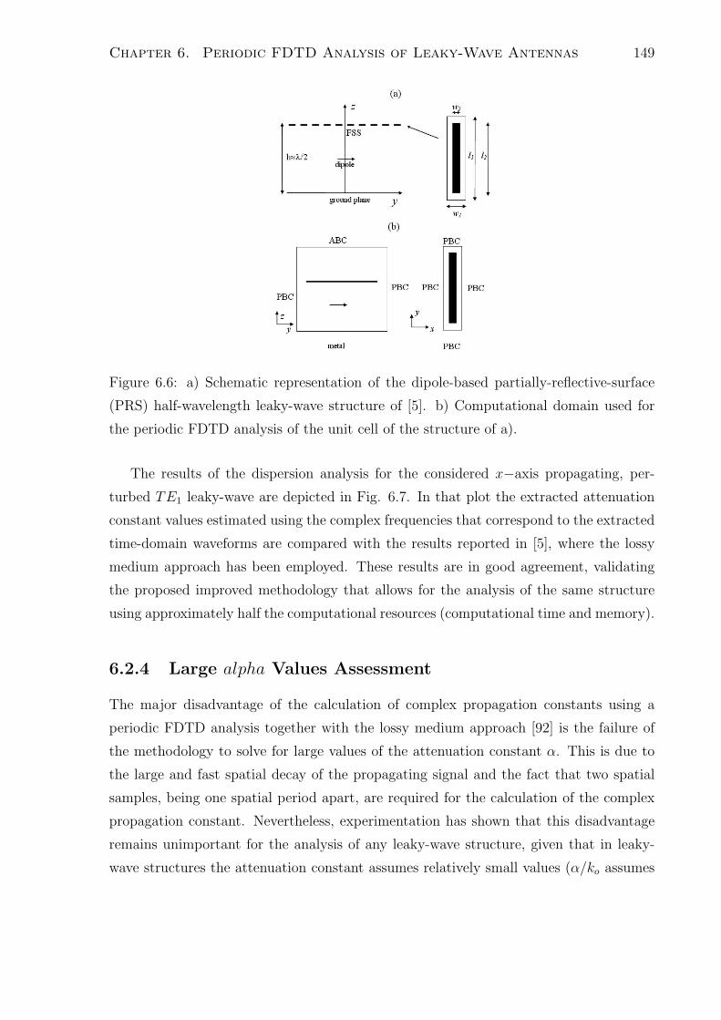
Chapter 6. Periodic FDTD Analysis of Leaky-Wave Antennas 149
Figure 6.6: a) Schematic representation of the dipole-based partially-reflective-surface
(PRS) half-wavelength leaky-wave structure of [5]. b) Computational domain used for
the periodic FDTD analysis of the unit cell of the structure of a).
The results of the dispersion analysis for the considered x−axis propagating, per-
turbed TE1 leaky-wave are depicted in Fig. 6.7. In that plot the extracted attenuation
constant values estimated using the complex frequencies that correspond to the extracted
time-domain waveforms are compared with the results reported in [5], where the lossy
medium approach has been employed. These results are in good agreement, validating
the proposed improved methodology that allows for the analysis of the same structure
using approximately half the computational resources (computational time and memory).
6.2.4 Large alpha Values Assessment
The major disadvantage of the calculation of complex propagation constants using a
periodic FDTD analysis together with the lossy medium approach [92] is the failure of
the methodology to solve for large values of the attenuation constant α. This is due to
the large and fast spatial decay of the propagating signal and the fact that two spatial
samples, being one spatial period apart, are required for the calculation of the complex
propagation constant. Nevertheless, experimentation has shown that this disadvantage
remains unimportant for the analysis of any leaky-wave structure, given that in leaky-
wave structures the attenuation constant assumes relatively small values (α/ko assumes

Chapter 6. Periodic FDTD Analysis of Leaky-Wave Antennas 150
14 16 18 200
0.05
0.1
0.15
0.2
0.25
Frequency (GHz)
β/k o
14 16 18 200
1
2
3
4
5
6x 10
−4
Frequency (GHz)
α/k o
Complex frequencyLossy medium
Figure 6.7: Complex propagation constant values of the perturbed, x−axis propagating
TE1 mode, calculated using the lossy medium approach [5] and the proposed improved
methodology.
values in the range of 10−5−10−3 in order for the resulting LWA to achieve high directivity
through the maximization of its effective radiating aperture). On the other hand, this
disadvantage becomes dominant when periodic structures are solved for evanescent modes
(e.g. in cases in which periodic structures are designed to be used as EBGs). This
suggestion had been also mentioned in [92], where the the proposed methodology had
failed to calculate the dispersion diagram of the unbalanced LC loaded transmission line
metamaterial within the formulated stopbands.
Given the fact that the improved methodology employs only one spatial sample of the
field, it is expected to exhibit an enhanced performance as far as the calculation of large
α values are concerned. In the following text, it is attempted to quantify this expectation
and quantitatively compare the two approaches by means of a numerical experiment. For
this purpose, an 1-D wave of the form of equation (6.9) is assumed.
A (x, t) = Aoe−j((β−jα)(x−xo)−ωr(t−to)) (6.9)
As shown above, this wave can be rewritten as
A (x, t) = Aoe−j(β(x−xo)−(ωr+j αωr
β )(t−to)) (6.10)
This wave is considered to be a leaky-wave (i.e. β < ko and α > 0) of radial frequency
ω = ωr, emanating from point x = xo at the time moment t = to. The attenuation

Chapter 6. Periodic FDTD Analysis of Leaky-Wave Antennas 151
10−3
10−2
10−1
100
0
2
4
6
8
10
12
14
16
α / ko (Np)
Err
or in
α c
alcu
latio
n (%
)
Complex FrequencyLossy Medium
Figure 6.8: Error in α calculation using the lossy medium approach the improved method-
ology as a function of the magnitude of α.
constant α is considered to be arbitrary large, while its exact value is being preset. To
make this ideal wave to resemble more a real-world wave, white Gaussian noise is added to
it so as its SNR level to be 40dB. This 1-D wave is sampled at points x = x1 and x = x2,
where x1−xo = 0.1λ and x2−x1 = 0.2λ (the first sampling point x = x1 is considered to
be very close to the source x = xo, while the second sampling point x = x2 is considered
to be λ/5 away from the first point, distance that could in many cases correspond to the
periodicity of a periodic EBG structure). Then, the two samples are employed together
with the lossy medium approach for the estimation of the preset attenuation constant
value while only the first sample is employed together with the improved methodology for
the estimation of the same attenuation constant value. The error between the calculated
values and the preset value of α is then estimated and the same experiment is repeated
for several growing α values. The results of this numerical experiment are reported in
Fig. 6.8. These results suggest that for small values of the attenuation constant α both
methods can effectively estimate it with an average error of 1 %. This error must be
attributed to the numerical errors involved in the implementation of the two methods.
Nevertheless, the error in the calculation of α when using the traditional lossy medium
approach starts increasing for values of α that are greater than 0.11ko. On the other
hand, the error remains bounded when the improved methodology is employed for values
of α as large as ko. Therefore, it is reasonable to suggest that the proposed improved
methodology may be used for the estimation of attenuation constant values that are 10
times larger that those that can be estimated using the lossy medium approach.

Chapter 6. Periodic FDTD Analysis of Leaky-Wave Antennas 152
6.3 Periodic FDTD Analysis of Sub-wavelength Res-
onant Cavity Type 2-D LWA
In this section, the periodic FDTD technique of [92] together with the proposed im-
proved methodology for the post-processing of the time-domain data and the calcula-
tion of the complex propagation constants of leaky-modes are employed for the anal-
ysis of a novel leaky-wave structure, namely, the sub-wavelength resonant cavity type
2-D LWA. The underlying operating concept for this class of antennas is similar with
any partially-reflective-surface cavity-type LWA, such the one analysed in the previous
section; the power leakage accompanying a perturbed parallel plate mode, supported
between a ground plane and a partially-reflective-surface, is exploited for the design of
highly-directive antennas. Nevertheless, the structures under consideration are of sub-
wavelength heights (instead of being of height λ/2, at which the first mode of a parallel
plate waveguide is supported). This is achieved with the use of artificial magnetic con-
ductors (AMCs) (or high impedance surfaces (HISs)) for ground planes instead of conven-
tional electric conductors. By properly setting the properties of the employed artificial
ground plane (the reflective coefficient of the AMCs or the impedance of the HISs), the
first cavity resonance between the PRS and the artificial ground plane is supported for
separations (cavity heights) much smaller than half-wavelength.
A schematic representation of the investigated sub-wavelength resonant cavity type
2-D LWA is depicted in Fig. 6.9. Specifically, in Fig. 6.9(a), where the side view of
the antenna is depicted, it can be seen that the antenna is mainly composed of a PRS,
printed on a free standing dielectric substrate, and a magnetic ground plane (MGP),
printed on a grounded dielectric substrate. These two surfaces, brought close to each
other (at distance h < λ/2), form a resonant cavity. As already mentioned, the resonant
height h is defined mostly by the properties of the MGP. In the following text, cavities of
different heights, PRSs and MGPs will be investigated. In Fig. 6.9(b) the top view of the
PRS is depicted. For the investigated antenna designs the PRS is composed of square
aperture patches (of length Lprs) arranged in 2-D periodic configurations (of spatial
period Dprs) and printed on low loss dielectric substrates. This substrate is considered
to be outside the cavity (just above the cavity) to minimize the dielectric losses of the
antenna. Finally, the top view of the of the employed MGP is shown in Fig. 6.9(c).
The MGP is composed of square patches (of length Lmgp) arranged in a 2-D periodic

Chapter 6. Periodic FDTD Analysis of Leaky-Wave Antennas 153
Figure 6.9: Schematic representation of the investigated sub-wavelength resonant cavity
type 2-D leaky-wave antennas. a) Cross-section of the investigated antennas, b)top-view
of the employed PRS and c) top-view of the employed MGP.
configuration (of spatial period Dmgp) and is printed on a grounded dielectric substrate.
Due to the strong fields that are supported in this substrate, the employed dielectric
substrate should be of minimal dielectric losses. The aforementioned dimensions of the
PRS and the MGP determine the electromagnetic properties of these two surfaces and
the LWA thereof. Specifically the dimensions related to the PRS define its reflection
coefficient and therefore the power leakage rate of the LWA. Those related to the MGP
define its reflection phase and by adjusting them different resonant cavity heights can be
achieved.
The purpose of the periodic FDTD analysis for this class of antennas is the investi-
gation of the impact of the cavity height to the complex propagation constants of the
supported leaky-modes, and, therefore, the optimization of the delivered directivity by an
antenna of a given physical aperture with respect to its cavity height. For this purpose,
several resonant cavity antennas of different cavity heights (and, therefore, of different
MGP parameters) are analysed and the supported complex propagation constants are
compared. A list of all the antenna structures that have been investigated is reported
in Table 6.3. It is pointed out that all these structures have been designed for opera-
tion at about 3.7 GHz. In all of them, the periodicity of both the PRS and the MGP

Chapter 6. Periodic FDTD Analysis of Leaky-Wave Antennas 154
are Dprs = Dmgp = 22 mm (Dprs, Dmgp ≈ 0.27λ), while the employed dielectric sub-
strates parameters in all of them are ǫr,prs = 2.46, hsub,prs = 3.198 mm, ǫr,mgp = 2.56,
hsub,prs = 3.152 mm.
Structure ID CavityHeight (mm) Lmgp (mm) ∠Lmgp (degrees)
λ/2 38.89 - -
λ/3 26.6 18.25 75.45
λ/3.9 20.9 19.03 15.67
λ/4.9 16.5 19.50 -33.43
λ/6.1 13.2 19.80 -62.05
λ/7.0 11.6 19.95 -74.33
λ/12.7 6.4 20.50 -107.92
λ/19.8 4.1 20.80 -120.67
Table 6.1: Cavity heights and MGP parameters of the investigated antenna structures.
Fig. 6.10 shows the cross-section of the computational domain that is used for the
periodic FDTD analysis of the sub-wavelength resonant cavity type 2-D LWAs. As
already suggested, this computational domain is comprised from a single unit cell of the
antenna and is terminated with PBCs at the planes of periodicity. A polarized line current
source along x−axis is employed to excite simultaneously TE modes along the z−axis and
TM modes along the x−axis. It is pointed out that, given that different discretization
(meshing) schemes were employed for each of the structures of Table 6.3, very dense
meshes, that would minimize the numerical error in each of them, were employed. The
need for extremely dense meshes was also imposed by the strong electric fields supported
within the resonating cavity and especially within the substrate of the MGP. Due to all
these reasons, the computational domain of Fig. 6.10 was composed of large numbers of
Yee’s cells (of the order of several millions). Therefore, the improved methodology that
allows for the calculation of the complex propagation constants using a single spatial
time-domain sample enabled and significantly accelerated the implementation of this
study.
The computational domain of Fig. 6.10 is initially employed for the analysis of four
of the antenna structures that are described in Table 6.3, namely the λ/2, the λ/4.9, the
λ/12.7 and the λ/19.8 . All these designs incorporate a PRS having a reflection coefficient
of 0.962 (i.e., Lprs = 14. mm). The results of the analysis of these four structures

Chapter 6. Periodic FDTD Analysis of Leaky-Wave Antennas 155
Figure 6.10: Side view of the computational domain employed for the periodic FDTD
analysis of the sub-wavelength resonant cavity type 2-D LWAs.
are depicted in Fig. 6.11 and Fig. 6.12. Specifically, Fig. 6.11 shows the section
of the dispersion diagram that corresponds to TE leaky-modes which only propagate
along the z−axis and are characterized by small phase constants (i.e., βd ≤ 15o ). The
reason for the latter restriction is that this analysis is focused on broadside radiators, and
broadside radiation occurs when |α| ≤ |β| . All of the four antennas support fast-waves
at approximately 3.7 GHz. It has to be pointed out that all the modes depicted in Fig.
6.11 are deep in the radiating region of the dispersion diagram, given the relatively large
periodicity of the antennas under investigation.
Based on simple inspection of the slope of the dispersion curves of Fig. 6.11, it is
concluded that the investigated antenna becomes more narrowband as the cavity height
is reduced. Therefore, the λ/19.8 resonant cavity antenna is the most narrowband of the
four structures considered, while the λ/2 antenna is the most broadband.
Fig. 6.12 depicts the attenuation constants associated with the fast-waves shown in
Fig. 6.11. Inspection of these results suggests that the attenuation constants do not
vary monotonically with the change of the cavity height. Instead, they decrease as the
cavity height is reduced from to λ/9 to λ/4.9. When the cavity height is reduced below
λ/4.9 the attenuation constants begin to increase again. This observation, motivated us
to extend our study to consider additional cavity heights, and further antenna designs
were investigated (i.e. all the antennas of Table 6.3, in conjunction with three different

Chapter 6. Periodic FDTD Analysis of Leaky-Wave Antennas 156
Figure 6.11: Phase constant of the sup-
ported TE leaky-modes.
Figure 6.12: Attenuation constants of
the leaky-modes shown in Fig. 6.11.
Figure 6.13: Normalized attenuation constant as a function of cavity height for three
different PRSs.
PRSs). The results of this study are presented in Fig. 6.13. Upon inspection of this
graph it is possible to precisely point out the cavity height which yields the smallest
attenuation constant. This height is of the order of λ/4.9. There is however a trend
for this optimum point to move towards lower cavity heights as the PRS reflectivity is
increased. It is expected, therefore, that for the first two PRS designs (those with reflec-
tivity |ΓPRS| = 0.901 and |ΓPRS| = 0.962) this cavity height will deliver the maximum
value of directivity. For a PRS reflectivity of 0.998 the optimum point occurs for a cavity
height of approximately λ/6.
All the aforementioned conclusions were validated through full-wave simulations of
antenna structures of finite lateral dimensions and were employed for the fabrication of
antenna prototypes with optimized (maximized) delivered directivities. Several of these
results have been presented in [6].

Chapter 6. Periodic FDTD Analysis of Leaky-Wave Antennas 157
6.4 Radiation Pattern Calculation of Finite-size LWAs
Using Periodic FDTD Simulations
6.4.1 General
Up to this point, the periodic FDTD technique together with the proposed improved
methodology for the post-processing of time-domain waveforms were presented and em-
ployed for the calculation of the complex propagation constants of the leaky-modes sup-
ported by sub-wavelength resonant cavity type 2-D LWAs. Although the values of the
complex propagation constants of the leaky-modes provide several indirect information
about the radiating properties of the considered structures, they can not provide di-
rectly their radiation patterns. For this reason, the development of a semi-analytical
formulation for the estimation of the expected radiation patterns of periodic, finite-size,
sub-wavelength resonant cavity type 2-D LWA, composed of sub-wavelength unit cells,
given the complex propagation constants of the supported modes is presented in this
section.
Under the effective aperture condition, any infinitely long 1 periodic LWA, composed
of unit cells of sub-wavelength dimensions, can be treated as a phased array [145], [146].
In that case, each cell of the antenna is assumed to be an omnidirectional point radiator
fed with a current of the form In = Ioe−nαde−jnβd, where γ = β − jα is the complex
propagation constant of the supported leaky-wave. That current value would correspond
to the magnitude of a traveling leaky-wave at the location of this unit cell. Therefore,
the total radiation pattern of the array is identical with the array factor of the equivalent
phased array (equation (6.11)) and is given by equation (6.12).
AF =N−1∑
n=0
Inejnkodcosθ (6.11)
AF =N−1∑
n=0
e−nαdejn(kodcosθ−βd) (6.12)
1A LWA can be assumed to be infinitely long when it is long enough to radiate all the power that isfed to it.

Chapter 6. Periodic FDTD Analysis of Leaky-Wave Antennas 158
6.4.2 Electromagnetic Behavior of Finite-size LWA
The attenuation constant of the supported leaky-waves α usually assumes extremely small
values and, therefore, in order for most of the power fed into the antennas to be radiated,
leaky-wave structures should be large in size (several wavelengths). In many practical
cases, this is not possible due to space/volume restrictions. Such is the case for the
sub-wavelength resonant cavity type 2-D LWA of the previous section; for an attenuation
constant of α = 0.01, in order for the 90% of the fed power to be radiated the structure
should be approximately 4.5 m long. This is not possible for an antenna operating at
3.7 GHz and being designed for use in commercial communications. Nevertheless, the
aforementioned antennas have been prototyped in reasonable lateral sizes (i.e. 29 cm,
13 unit cells) and have been measured to deliver high gains corresponding to aperture
efficiencies of the order of 50% or more [6], [5]. Therefore, the question to be answered is
how such high aperture efficiencies are achieved by antennas of finite and compact lateral
size.
(z)
(x)
• TE-waves • H-plane
• TM-waves • E-plane
Dz
Dx
Figure 6.14: Top view of a finite size resonant cavity type 2-D LWA. If the structure
is excited with an x−axis oriented current source, a TE wave will be supported along
z−axis and a TM wave along x−axis. The TE wave will correspond the yz−plane to the
H-plane of the antenna and the TM wave would create an E-plane in the xy-plane.
In order to answer this question, let us use the resonant cavity type 2-D LWA as a
driving example and consider the leaky-modes supported in these structures. In Fig. 6.14
the top view of a square, periodic resonant cavity type 2-D LWA with finite dimensions

Chapter 6. Periodic FDTD Analysis of Leaky-Wave Antennas 159
Dz and Dx is depicted. If this structure is excited with an x−oriented line source, the
fundamental established modes will be a TE wave along z−axis and a TM wave along
x−axis. These waves are in principle perturbations of the TE and TM modes supported
by parallel plate waveguides (PPW) [5]. Therefore the impedance of these two modes
can be approximated by the impedances of the unperturbed modes
ZTM,perturbed ≈ ZTM,PPW =β (ω)
ωǫ(6.13)
ZTE,perturbed ≈ ZTE,PPW =ωµ
β (ω)(6.14)
where β (ω) =√
ω2ǫµ − (nπ/h) is the dispersion relation of the unperturbed modes and
ǫ, µ the parameters of the materials filling the cavity. When the perturbed TE and TM
waves are excited with small phase velocities βTM,perturbed −→ 0 and βTE,perturbed −→ 0
(very close to the cut-off frequency of the mode), equations (6.13) and (6.14) suggest that
ZTM,perturbed −→ 0 and ZTE,perturbed −→ ∞. In that case, the TM leaky-waves supported
by the open resonant cavity type 2-D leaky-wave structure will propagate through a very
small impedance and the corresponding TE leaky-waves through a very high impedance.
This is depicted in Fig. 6.15 and Fig. 6.16 where the analytical dispersion relations and
the corresponding impedances of the TE1 and TM1 modes supported by a λ/2 parallel
plate waveguide with a cut-off frequency at 3.7 GHz have been plotted.
Going back to the motivating example of the resonant cavity type 2-D LWA of Fig.
6.14, when the perturbed TM waves, that propagate along the x−axis through a low
impedance, and the perturbed TE waves, that propagate along the z−axis through a
high impedance, reach the edges of the finite-size structure, they face free space and a
medium impedance of 120πΩ. Because their characteristic impedances are much different
than the free space impedance, both waves will be reflected back in the structure and will
start traveling towards the opposite directions. If we ignore any diffraction effects that
might appear when the traveling waves reach the edges of the structure, the reflection
coefficients for both the TM and TE waves at the edges of the structure are presented in
Fig. 6.17. These results suggest that the TM waves are reflected with a positive coefficient
RTM that assumes the maximum value of unity at cut-off (when ZTM,perturbed −→ 0 ) and
decays away from cut-off. On the other hand, the TE waves are reflected with a negative
coefficient RTE that again assumes the maximum magnitude of unity at cut-off (when
ZTE,perturbed −→ ∞) and decays away from cut-off. In other words, the open edges of
the finite size structure act as shorts (electric walls) for the impinging TE waves and as

Chapter 6. Periodic FDTD Analysis of Leaky-Wave Antennas 160
0 0.5 1 1.5 23
3.5
4
4.5
5
Phase Velocity (rad/m)
Fre
quen
cy (
GH
z)
βTM
1
βTE
1
Figure 6.15: Dispersion relations of the
TE1 and TM1 modes supported by a
λ/2 parallel plate waveguide with a cut-
off frequency at 3.7 GHz
0 1000 2000 3000 4000 50003
3.5
4
4.5
5
Impendance (Ohms)
Fre
quen
cy (
GH
z)
ZTM
1
ZTE
1
Figure 6.16: Impedances of the TE1 and
TM1 modes supported by a λ/2 parallel
plate waveguide with a cut-off frequency
at 3.7 GHz.
opens (magnetic walls) for the TM waves.
Based on this analysis, it is concluded that in a finite size resonant cavity type 2-
D leaky-wave structure, such as that of Fig. 6.14, traveling waves are bouncing back
and forth, being reflected whenever they impinge on an open edge. Between any two
consecutive reflections they remain leaky, radiating power towards y−axis. Therefore, in
configurations like that of Fig. 6.14, traveling leaky-waves form after multiple reflections
a standing field distribution in the structure, and, hence, the radiating properties of the
structure (i.e. aperture efficiency, radiation patterns) should be attributed more to that
standing field distribution than to a single conventional, traveling leaky-wave.
6.4.3 Array Factor of Finite-size LWA
Proposed Model
Given the analysis of the previous section it becomes clear that equation (6.12) can
not be employed, under the effective aperture approach, for the calculation of the ra-
diation patterns of finite size LWAs, when the complex propagation constants of the
supported modes are known. This is because equation (6.12) considers conventional
traveling leaky-waves and, hence, excitation currents for the point radiators of the form

Chapter 6. Periodic FDTD Analysis of Leaky-Wave Antennas 161
−1 −0.5 0 0.5 13
3.5
4
4.5
5
Reflection Coef.F
requ
ency
(G
Hz)
RTM
1
RTE
1
Figure 6.17: Reflection coefficients for the TE and TM wave impinging at the open ends
of a finite size waveguide structure (with a cut-off frequency at 3.7GHz), when diffraction
effects are not considered.
Io
I0 I1 I-1 I2 I-2 I-n I-(N-1)/2 I(N-1)/2 In
R R
In,dir
In,indir
d
Figure 6.18: Array representation of a cross section of a finite size LWA along any of its
principal planes.
In = Ioe−nαde−jnβd. On the contrary, it is suggested hereby, that the generic array factor
equation (6.11) could be used for the calculation of the radiation patterns of finite-size
LWAs, at least at the principal radiation planes of the antenna, provided that the correct
current coefficients In that correspond to each of the unit cells along these planes are
calculated in accordance with the analysis of the previous section. That calculation of
the current coefficients is attempted in the following text.
For this purpose, let us consider an 1-D array of N point radiators (N is considered
to be an odd number) terminated at both edges with reflective surfaces of reflection coef-
ficient R, as shown in Fig. 6.18. These point radiators correspond to the sub-wavelength
unit cells of the finite-size LWA under investigation, R corresponds to the reflection co-
efficient facing the traveling leaky-waves when reaching the edges of the structure, while
Chapter 6. Periodic FDTD Analysis of Leaky-Wave Antennas 162
the entire array can be representative of any principal planes cross sections of the LWA.
Assuming that the array is externally fed at its middle element with a current Io (feed-
ing point of the LWA), traveling leaky-waves will be excited towards both directions of
the array, with respect to the middle element (left and right). Each of these two waves
will be consecutively reflected whenever it reaches any edge of the array and eventually a
standing field distribution will be created. For the estimation of the equivalent excitation
currents of the array elements, it is considered that the total current of the nth−radiator
In is consisted of two components; the first is derived from the wave the directly arrives at
this unit cell from the feeding point of the array and the multiple reflections of that wave,
and the second is derived from that wave that originally traveled towards the opposite
direction and indirectly reached that unit cell after a single reflection at the opposite
edge, and the multiple reflections of that wave. This is also shown in Fig. 6.18, and can
be expressed as
In = In,dir + In,indir (6.15)
The component In,dir of equation (6.15) can be expressed in terms of the array pa-
rameters and the complex propagation constant of the examined leaky-waves as
In,dir = I+n +I+
n
(
Φ+RΦ+)
+I+n
(
Φ+RΦ+) (
Φ−RΦ−)
+I+n
(
Φ+RΦ+) (
Φ−RΦ−) (
Φ+RΦ+)
+...
(6.16)
where I+n is given by equation (6.17) and corresponds to the wave that directly reaches
the nth unit cell from the feeding point, the second term of equation (6.16) corresponds
to the first reflection of I+n to the closest reflection surface, the third term of equation
(6.16) corresponds to the second reflection of I+n to the opposite reflection surface etc.
The coefficient Φ+ is the transmission coefficient (phasor) of a wave traveling from the
nth element to the nearest reflecting surface and is given by equation (6.18), and Φ− is the
transmission coefficient of a wave traveling from the nth element to the other (opposite)
reflecting surface and is given by equation (6.19)
I+n = Ioe
−jn(β−jα)d (6.17)
Φ+n = e−j(N−1
2−n)(β−jα)d (6.18)
Φ−
n = e−j(N−1
2+n)(β−jα)d (6.19)
Similarly, the contribution of the indirect component involved in equation (6.15) can
Chapter 6. Periodic FDTD Analysis of Leaky-Wave Antennas 163
be written as
In,indir = I−
n +I−
n
(
Φ+RΦ+)
+I−
n
(
Φ+RΦ+) (
Φ−RΦ−)
+I−
n
(
Φ+RΦ+) (
Φ−RΦ−) (
Φ+RΦ+)
+...
(6.20)
where I−
n corresponds to the indirect wave that reaches the nth radiatos and is given by
equation (6.21).
I−
n = Ioe−j(N−1
2)(β−jα)dΦ−
n (6.21)
Combining equation (6.15) with equations (6.16) and (6.20), the total current on the
nth element of the array can be written as
In =∞∑
m=0
(
I+n + I−
n
) [
Φ+n RΦ+
n
]m [
Φ−
n RΦ−
n
]m+
∞∑
m=1
(
I+n + I−
n
) [
Φ+n RΦ+
n
]m [
Φ−
n RΦ−
n
](m−1)
(6.22)
Equation (6.22) can be then used together with the conventional generic array factor
equation (6.11) for the calculation of the principal planes radiation patterns of finite size
LWAs.
Validation - Discussion
For the validation of the proposed model, the principal radiation patterns of a sub-
wavelength finite size resonant cavity type 2-D LWA are calculated, using the proposed
model together with the FDTD results reported in section 6.3, and are compared with the
corresponding radiation patterns, obtained through the simulation of the entire finite-size
structure using a commercial full-wave EM solver (CST Microstripes), that have been
reported in [6].
The antenna under consideration is a λ/4.9 resonant cavity type 2-D LWA composed
of 13 unit cells, identical with that of Fig. 6.10, along both principal planes (the antenna
is composed of 132 unit cells in total). The reflection coefficient of the employed PRS
has been considered to be ΓPRS = 0.962, while the periodicity of the structure is d =
22 mm in both principal planes. This unit cell has been analysed in section 6.3 and the
supported complex propagation constants derived by its periodic FDTD analysis have
been presented in Fig. 6.11 and Fig. 6.12.
Using the proposed model (with RE−plane = 1 and RH−plane = −1), the aforemen-
tioned parameters and the results of the periodic FDTD analysis of the unit cell, the
calculated E- and H-plane radiation patterns are presented in Fig. 6.19.

Chapter 6. Periodic FDTD Analysis of Leaky-Wave Antennas 164
−80 −60 −40 −20 0 20 40 60 80−40
−35
−30
−25
−20
−15
−10
−5
0
Angle (degrees)
Nor
mal
ized
Am
plitu
de (
dB)
H−planeE−plane
Figure 6.19: E- and H-plane radiation patterns of a λ/4.9 resonant cavity type 2-D
leaky-wave antenna composed of 13 unit cells, calculated using the proposed model.
Figure 6.20: E- and H-plane radiation patterns of a λ/4.9 resonant cavity type 2-D leaky-
wave antenna composed of 13 unit cells, calculated using the a full-wave simulation of
the entire finite size structure (obtained from [6]).

Chapter 6. Periodic FDTD Analysis of Leaky-Wave Antennas 165
In Fig. 6.20 the radiation patterns of the same structure, calculated using CST Mi-
crostripes and originally reported in [6], are depicted. Comparing the radiation patterns
of Fig. 6.19 and Fig. 6.20 good agreement can be observed. The E-plane radiation
pattern calculated using the proposed model achieves the same number of nulls and at
roughly the same angles with that calculated through the full-wave simulation. The side-
lobe level and the endfire radiation in both patterns are of the same order of magnitude
(roughly −13 dB and −19 dB, respectively), while similar directivity values can be ex-
tracted from both patterns. Good agreement is also observed for the H-plane patterns.
In that case, both the full-wave and the array factor patterns exhibit two nulls left and
right of the broadside direction, both patterns exhibit a sidelobe level of the order of
−23 dB and endfire directivity of the order of −28 dB, and both patterns suggest that
the H-plane pattern of the investigated antenna is less directive than its E-plane pattern.
Nevertheless, between the two sets of patterns there are also some disagreements,
mostly related with the exact position and the depth of the nulls. This disagreement is
attributed to the fact that no diffraction effects have been considered in the proposed
model for the calculation of the radiation patterns. In fact, diffraction is expected to
affect the total radiation patterns of the finite-size antenna in two different ways. First,
due to the diffraction of waves at the open edges, the reflection coefficient encountered
by the traveling leaky-waves when reaching the edges of the structure would deviate
form the ideal values of RE−plane = 1 and RH−plane = −1 that were considered in the
proposed model. This deviation concerns both the magnitude of the reflection coefficients
(they are expected to be less than the unity) and also its phase (due to the diffraction,
the reflection coefficients are expected to possess some small imaginary part). Secondly,
the diffracted power at the edges of the finite-size structure is also radiated in the free
space and is part of the total radiation patterns that are calculated with the full-wave
simulation of the finite structure. Therefore, the patterns of Fig. 6.20 also include the
contributions of the diffracted fields, while those of Fig. 6.19 were derived by considering
only radiated from the array fields.
Conclusively, even though the proposed model is inherently an approximate one, it
could be used to some extend for the fast and analytical calculation of the radiation
patterns of finite-size LWAs. For the calculation of these patterns, only the complex
propagation constants of the supported leaky-waves, that can be extracted using the
proposed single-cell periodic FDTD methodology, are required. The benefit of using this
model may be huge as the full-wave simulation of the entire finite-size LWA may require

Chapter 6. Periodic FDTD Analysis of Leaky-Wave Antennas 166
several hours of computational time and significantly large computational resources.

Chapter 7
Conclusions
7.1 Review
In this thesis, the analysis, design and modeling of novel metamaterial and metamaterial-
inspired microwave structures and antenna applications were presented. Motivated by the
challenge of enhancing the penetration of metamaterial-related applications into commer-
cial products, novel, low cost, easily deployable metamaterial structures were proposed.
Such metamaterial structures were employed for the design of easily fabricated antenna el-
ements and arrays of those. Also, a periodic, full-wave, FDTD-based tool was developed,
optimized and linked to novel post-processing algorithms that enabled the computation-
ally efficient, rigorous and inclusive characterization of high-gain, metamaterial-based,
flat-plate antennas.
In chapter 2, all the theoretical aspects that were employed throughout the thesis
were presented. Specifically, all the possible approaches for the synthesis of metamaterial
structures were briefly described and modeled through the equivalent circuit analysis of
resonators either interacting with impinging plane waves or forming arrays of tightly
coupled unit cells. It was shown that the latter approach, that has been much less
investigated in the literature, can be employed for the synthesis of any of the well-known
metamaterial properties and applications, depending on the magnitude and the nature
of the coupling between the resonators. Also, in the same chapter, all the theoretical
background of the in-house periodic FDTD-based computational tool, that has been
extensively employed and furthered developed in this thesis, was briefly presented.
In chapter 3, the theory for the design of metamaterial structures employing tightly
coupled resonators was employed together with compact resonators printed on grounded
167

Chapter 7. Conclusions 168
dielectric substrates for the synthesis of microstrip-based artificial transmission lines and
applications of those. Specifically, the double-spiral resonator (DSR) was identified as a
proper modular element for the design of such lines, was extensively analysed and all its
unique properties were identified. In turn, such resonators were employed for the design
of DSR-based artificial lines supporting backward waves over a measured fractional band-
width of 13%. Such lines were used for the synthesis of broadband series-fed microstrip
patch arrays, exhibiting reduced sidelobe levels and beam-scanning capabilities.
In chapter 4, tightly coupled resonators were employed in non-grounded configura-
tions for the synthesis of compact, phase-shifting lines that were used for the design of
low-profile folded monopoles. In the proposed approach, two low-profile, vertical, radi-
ating posts were connected through an artificial, non-radiating, phase-shifting line that
was used to enforce the resonance condition of conventional folded monopoles. Therefore,
the resulting radiators were self-resonant while they exploited the four-fold increase of
the radiation resistance of folded monopoles to exhibit decent radiation resistances even
though being of low profile. Such monopoles were explicitly modeled and analysed, radi-
ators of different profiles were investigated while the impact of the ground plane against
which they were fed was also studied. Both coaxially and microstrip-fed monopoles were
considered while it was shown that pairs of such monopoles exhibit reduced electromag-
netic coupling as compared to the coupling between conventional quarter-wavelength
monopoles.
The self-resonant, low-profile, low-coupling monopoles of chapter 4 were employed in
chapter 5 for the design of two classes of sub-wavelength antenna arrays. The first of them
was a two-element phased array in which the array element separation was approximately
λ/5. Even that small inter-element separation the measured performance of the array was
close to the theoretically expected, in contrast to the performance of the corresponding
array of conventional monopoles. The second class of sub-wavelength arrays that were
investigated were two-element superdirective endfire arrays. In that case, the inherent
properties of the employed low-profile folded monopoles enabled the simplification of the
required feeding network and the fabrication of single-port microstrip-based arrays. The
directivity and the gain delivered by such arrays were rigorously measured to validate
both their superdirective properties and the fundamental limitations associated with their
operation. In the same chapter, a metamaterial-inspired decoupling mechanism was
proposed for the coupling reduction between conventional planar inverted-F antennas
participating in compact arrays built on a common ground plane (handheld devices).

Chapter 7. Conclusions 169
According to this scheme, a resonating pair of slits (effective magnetic loop) was added
in the coupling path between the two coupled antennas to insert a transmission-zero.
The last chapter of the thesis was dedicated to the numerically efficient modeling
of periodic leaky-wave structures with emphasis to metamaterial-based high-gain leaky-
wave antennas. The periodic in-house FDTD-based tool of [92] was linked with novel
post-processing algorithms that enabled the reduction of the computational resources
required for the analysis of periodic leaky-wave structures. The numerically improved
methodology was employed for the analysis of novel sub-wavelength resonant cavity type
2-D leaky-wave antennas and the optimization of their directivity with respect to their
profile. Finally, post-processing algorithms that allowed the approximate calculation of
radiation patterns of electrically large, finite-size, 2-D leaky-wave antennas through the
periodic FDTD analysis of their unit cell were developed.
7.2 Future Work
The objective of this thesis was to propose novel, low-cost, easily fabricated metamate-
rial structures that could be easily deployed within commercial microwave applications.
For this purpose, the least investigated class of metamaterial structures, those formed
by arrays of tightly coupled resonators, was employed. The outcomes of this research
endeavor include several interesting metamaterial structures that could be deployed in
several commercial applications given that they address many of the requirements of
modern telecommunication systems such as size/volume reduction, low fabrication cost
and compatibility with standard microwave technologies. For this reason, it is believed
that this research endeavor could potentially inspire future research activity targeting at
the development and validation of more metamaterial-based microwave applications. In
the following text, some of the directions of future research related with the context of
this thesis are briefly presented.
First, on the front of the synthesis of metamaterial structures using tightly coupled
resonators, it would be interesting if the coupling requirements for the synthesis of differ-
ent metamaterial properties could be married with traditional filter synthesis theory [32].
The results of this study should comment on which of the metamaterial properties could
be achieved under the restrictions imposed by the filter synthesis theory on the sign of
the coupling coefficients. Then, these metamaterial properties could be synthesised over
an exact and predefined bandwidth.

Chapter 7. Conclusions 170
On the front of the design of microstrip-based artificial lines, the use of different
resonators for the synthesis of such lines may be worth investigating. Even though the
double-spiral resonator investigated in this thesis exhibits several comparative advantages
(small footprint, discrete inductive components) it does not provide a direct means of
reconfiguring its electromagnetic properties (e.g. through a tuning discrete component
such a varactor or a PIN diode). This is mostly due to the fact that it does not possess a
discrete capacitive gap on which a tuning discrete element could be fit. Therefore, future
research on reconfigurable resonators and how they could be employed for the synthesis
of artificial lines could lead to the design of novel reconfigurable metamaterial structures.
Regarding the proposed low-profile folded monopoles, future research work may in-
volve the implementation of these monopoles in planar form, using both single layer and
multilayer PCB technology. Some initial investigations carried out showed that such im-
plementations are definitely possible. In their planar form, such antennas could be also
considered for applications that require integrated, fully-printed, electrically small radi-
ators. Also, in their planar form, such monopoles could be designed in dually-polarized
configurations. Another promising feature of the proposed low-profile folded monopoles
is that their radiating mechanism is to a certain degree decorrelated to their reactive
components. Therefore, the self-resonance of such monopoles can be tunned only by
tunning the properties of the embedded matching network (phase-shifting line). As a
result, it is reasonable to expect that reconfigurable folded monopoles could be easily
designed if reconfigurable coupled resonators were employed as embedded phase-shifting
lines. Also, regarding the arrays of low-profile folded monopoles, given the comparative
advantages of such monopoles when forming compact arrays (reduced mutual coupling,
robust input impedance), it would be interesting to test such compact arrays within an
experimental MIMO setup in order to experimentally assess the capacity gain obtained
by employing such sub-wavelength arrays.
Finally, on the front of the periodic modeling of electrical large, metamaterial-based,
high-gain antennas, it is strongly believed that most of the identifying antenna parameters
of such radiators can be rigorously obtained by the full-wave periodic analysis of a single
unit-cell and the post-processing of the extracted data. Therefore, more post-processing
algorithms, similar with those presented in this thesis, should be developed and employed
together with the periodic analysis to achieve the computationally efficient analysis of
these antennas. For example, such post-processing algorithms may be developed for the
calculation of the impedance characteristics of an antenna, its effective aperture and its

Chapter 7. Conclusions 171
radiation efficiency. For the improvement of the accuracy of all these algorithm the effect
of the diffraction at the edges of the finite-size antenna should be also modeled and taken
into account.

Appendix A
Analysis Of Coupled Lines
Any pair of microstrip lines that are located close to each other can be assumed to
be coupled. In this case, the electrical characteristics of these lines, for TEM type of
propagation, can be completely determined in terms of the phase velocity supported by
each line and the effective capacitances between them.
In the following, two different extreme types of excitations for the coupled lines are
examined. The first type refers to the case in which the currents on the coupled strips
are equal in magnitude and in the same direction. This type of coupled line is shown
in Figure A.1 and is referred in the literature as even-mode excited lines. In this case,
a hypothetical magnetic wall can be assumed between the two lines, no displacement
currents and no effective capacitance are supported between the lines, and, consequently,
the propagation on each line is defined by the characteristics of each line.
The second type of excitation is the odd-mode excitation, in which the currents on
the lines are of the same magnitude but are flowing in opposite directions. This case is
depicted in Figure A.2.
Under an odd-mode excitation, a hypothetic electric wall can be assumed between the
lines and the coupling between the lines can be modeled through a capacitance between
the strips. This capacitance can be expressed in terms of the parallel combination of a
capacitance that represents the fringing fields within the dielectric substrate just below
the strips (Cgd/2 in Figure A.2) with the capacitance that represents the fringing fields
in the air just above them Cga/2 in Figure A.2). Each one of these two capacitances are
expressed as a series combination of two capacitors (Cgd and Cga, respectively), while the
mutual poles of these capacitors are grounded, due the created electric wall. Therefore,
all the capacitances of Figure A.2 are grounded.
172

Appendix A. Analysis Of Coupled Lines 173
w s
I I
h εr
εο
Magnetic wall
cp cp
w
Figure A.1: Microstrip lines coupled under an even-mode excitation. In that case a mag-
netic wall can be assumed between the lines and, therefore, no capacitance is supported
between them.
w s
cga
cgd
cga
cgd
I -I
h εr
εο
Electric wall w
cp cp
Figure A.2: Microstrip lines coupled under an odd-mode excitation. In that case an
electric wall can be assumed between the lines and, therefore, a fringing field capacitance
is supported between them.

Appendix A. Analysis Of Coupled Lines 174
To conclude the analysis of the coupled lines under an odd-mode excitation, the values
of the aforementioned capacitances should be estimated. For this purpose, in this study,
the semi-empirical formulas of [147] are employed.
According to the analysis of [147], the fringing fields capacitances for the air is given
by the equation
Cga = ǫo
K(k′)
K(k)(A.1)
where,
k =s/h
s/h + 2w/h(A.2)
and
k′ =√
1 − k2. (A.3)
Then, the ratio of the elliptic function of equation A.1 depends on the value of k.
Specifically,
K(k′)
K(k)=
1
πℓn
(
21 +
√k′
1 −√
k′
)
, if 0 ≤ k2 ≤ 0.5 (A.4)
andK(k′)
K(k)=
π
ℓn
2(
1 +√
k)
/(
1 −√
k) , if 0.5 ≤ k2 ≤ 1 (A.5)
Finally, the fringing field capacitances on the dielectric are given by equation A.6
Cgd =ǫoǫr
πℓn
coth(π
4
s
h
)
+ 0.65Cf
(
0.02
s/h
√ǫr + 1 − ǫ−2
r
)
(A.6)
where
Cf =
√ǫeff
2cZ0
− Cp
2(A.7)
and
Cp = ǫoǫr
w
h. (A.8)

Bibliography
[1] A. Taflove and S. C. Hagness, Computational Electrodynamics: The Finite-
Difference Time-Domain Method, 2nd ed. Boston: Artech House, 2000.
[2] A. Grbic and G.V Eleftheriades, “Periodic analysis of a 2-D negative refractive in-
dex transmission line structure,” IEEE Microwave Wireless Compon. Lett., vol. 51,
no. 10, pp. 2604–2611, Oct. 2003.
[3] J.B. Pendry, A.J. Holden, A.J. Robbins, and W.J. Stewart, “Magnetism from
conductors and enhanced nonlinear phenomena,” IEEE Trans. Microwave Theory
Tech., vol. 47, no. 11, pp. 2075–2084, Nov. 1999.
[4] A.I. Uzkov, “An approach to the problem of optimun directive antennae design,”
Comptes Rendus Academ. Sci. USSR, vol. 53, pp. 35–38, 1946.
[5] P. Kosmas, A.P. Feresidis, and G. Goussetis, “Periodic FDTD analysis of a 2-D
leaky-wave planar antenna based on dipole frequency selective surfaces. ,” IEEE
Trans. Antennas Propagat., vol. 55, no. 6, pp. 2006–2012, Jul. 2007.
[6] J.R. Kelly, T. Kokkinos, and A.P. Feresidis, “Analysis and design of sub-wavelength
resonant cavity type 2-D leaky-wave antennas ,” IEEE Trans. Antennas Propagat.,
vol. 56, no. 9, pp. 2817–2825, Sept. 2008.
[7] V.G. Veselago, “The electrodynamics of substances with simultaneously negative
values of ǫ and µ ,” Soviet Physics Uspekhi, vol. 10, no. 4, pp. 509–514, Jan-Feb
1968.
[8] R. Collin, Foundations For Microwave Engineering, 2nd ed. Toronto, ON:
McGraw-Hill Inc., 1992.
175

Bibliography 176
[9] W. Rotman, “Plasma simulation by artificial dielectrics and parallel-plate media,”
IRE Trans. on Ant. and Propag., vol. 10, no. 1, pp. 82–95, Jan. 1962.
[10] J.D. Joannopoulos, S.G. Johnson, J.N. Winn, and R.D. Meade, Photonic Crystals:
Molding the Flow of Light, 2nd ed. New Jersey: Princeton University Press., 2008.
[11] J. B. Pendry, “Calculating photonic band structure,” J. Phys. : Condens. Matter,
vol. 9, Feb. 1996.
[12] E. Yablonovitch, “Photonic Crystals: Semiconductors of Light ,” Scientific Amer-
ican, pp. 47–55, Dec. 2001.
[13] M.M. Sigalas, C.T. Chan, K.M. Ho, and C.M. Soukoulis, “Metallic photonic band-
gap materials,” Phys. Rev. B, vol. 52, no. 16, pp. 11 744–11 752, Oct. 1995.
[14] A.S. Barlevy, D. Sievenpiper, and Y. Rahmat-Samii, “Photonic bandgap (PBG)
structures of multiple metallic periodic screens: efficient electromagnetic charac-
terization,” in Proc. IEEE Antennas and Propagation International Symposium
(AP-S), vol. 2, Jun. 1998, pp. 1216–1219.
[15] D. Sievenpiper and E. Yablonovitch, “Eliminating surface currents with metal-
lodielectric photonic crystals,” in Proc. IEEE International Microwave Symposium
(MTT-S), vol. 2, Jun. 1998, pp. 663–666.
[16] B.A. Munk, Frequency Selective Surfaces: Theory and Design, 1st ed. New York:
John Wiley and Sons, Ltd., 2000.
[17] J.C. Vardaxoglou, Frequency Selective Surfaces: Analysis and Design , 1st ed.
Research Studies Press Ltd, 1997.
[18] P.-S. Kildal, “Artificially soft and hard surfaces in electromagnetics,” IEEE Trans.
Antennas Propagat., vol. 38, no. 10, pp. 1537–1544, Oct. 1990.
[19] F. Mariotte, S.A. Tretyakov, and B. Sauviac, “Modeling effective properties of
chiral composites,” IEEE Antennas Propagat. Mag., vol. 38, no. 2, pp. 22 – 32,
Apr. 1996.
[20] N. Engheta, D.L. Jaggard, and M.W. Kowarz, “Electromagnetic waves in Faraday
chiral media,” IEEE Trans. Antennas Propagat., vol. 40, no. 4, pp. 367 – 374, Apr.
1992.

Bibliography 177
[21] F. Mariotte and N. Engheta, “Reflection and transmission of guided electromag-
netic waves at an air-chiral interface and at a chiral slab in a parallel-plate waveg-
uide,” IEEE Trans. Microwave Theory Tech., vol. 41, no. 11, pp. 1895–1906, Nov.
1993.
[22] J.B. Pendry, A.J. Holden, W.J. Stewart, and I. Youngs, “Extremely Low Frequency
Plasmons in Metallic Mesostructures,” Phys. Rev. Lett., vol. 76, p. 47734776, Jun.
1996.
[23] D.R. Smith, W.J. Padilla, D.C. Vier, S.C. Nemat-Nasser, and S. Schultz, “Compos-
ite Medium with Simultaneously Negative Permeability and Permittivity,” Phys.
Rev. Lett., vol. 84, no. 18, pp. 4184–4187, May 2000.
[24] R.A. Shelby, D.R. Smith, and S. Schultz, “Experimental verification of a negative
index of refraction,” Science Magazine, vol. 292, pp. 77–79, Apr. 2001.
[25] R.W. Ziolkowski and F. Auzanneau, “Artificial molecule realization of a magnetic
wall,” J. Appl. Phys, vol. 82, no. 7, pp. 3192 – 3194, Oct. 1997.
[26] ——, “Passive artificial molecule realizations of dielectric materials,” J. Appl. Phys,
vol. 82, no. 7, pp. 3195 – 3198, Oct. 1997.
[27] D. Sievenpiper, Z. Lijun, R.F.J. Broas, N.G. Alexopolous, and E. Yablonovitch,
“High-impedance electromagnetic surfaces with a forbidden frequency band,” IEEE
Trans. Microwave Theory Tech., vol. 47, no. 11, pp. 2059–2074, Nov. 1999.
[28] G.V. Eleftheriades, A.K Iyer, and P.C Kremer, “Planar negative refractive index
media using periodically L-C loaded transmission lines,” IEEE Trans. Microwave
Theory Tech., vol. 50, no. 12, pp. 1494–1504, Dec. 2002.
[29] G.V. Eleftheriades and K.G. Balmain, Negative-Refraction Metamaterials; Funda-
mental Principles and Applications. Hoboken, NJ: John Wiley and Sons, Inc.,
2005.
[30] A. Lai, T. Itoh, and C. Caloz, “Composite right/left-handed transmission line
metamaterials,” IEEE Microwave Magazine, vol. 5, no. 3, pp. 34–50, Sept. 2004.
[31] S. Ramo, J.R. Whinnery, and T. Van Duzer, Fields and Waves in Communication
Electronics, 3rd ed. New York, NY: John Wiley and Sons, Inc., 1994.

Bibliography 178
[32] J.S. Hong and M.J. Lancaster, Microstrip filters for RF microwave applications,
2nd ed. West Sussex, UK: John Wiley and Sons, Ltd., 2001.
[33] A.K. Iyer and G.V. Eleftheriades, “Negative refractive index metamaterials sup-
porting 2-D waves,” in Proc. IEEE Intl. Symp. on Microwave Theory and Tech.,
vol. 2, Seattle, WA, July 2002, pp. 1067–1070.
[34] S.M. Rudolph and A. Grbic, “Volumetric negative refractive index medium exhibit-
ing broadband negative permeability,” J. Appl. Phys., vol. 102, p. 013904 013906,
Jul. 2007.
[35] A.K Iyer and G.V. Eleftheriades, “A three-dimensional isotropic transmission-line
metamaterial topology for free-space excitation,” J. Appl. Phys., vol. 92, no. 26,
pp. 261 106 – 261 108, Jun. 2008.
[36] J.M. Williams, “Some Problems with Negative Refraction,” Phys. Rev. Lett.,
vol. 87, no. 24, p. 249703, Dec 2001.
[37] G.W.’t Hooft, “Comment on ‘Negative Refraction Makes a Perfect Lens’,” Phys.
Rev. Lett., vol. 87, no. 24, p. 249701, Dec 2001.
[38] N. Garcia and M. Nieto-Vesperinas, “Left-Handed Materials Do Not Make a Perfect
Lens,” Phys. Rev. Lett., vol. 88, no. 20, pp. 207 403–207 407, May 2002.
[39] ——, “Is there experimental verification of a negative index of refraction yet?”
Opt. Lett., vol. 27, no. 11, pp. 885–887, Jun. 2002.
[40] B.E. Spielman, S. Amari, C. Caloz, G.V. Eleftheriades, T. Itoh, D.R. Jackson, R.
Levy, J.D. Rhodes, and R.V. Snyder, “Metamaterials: A Rich Opportunity for
Discovery or an Overhyped Gravy Train,” IEEE Microwave Magaz., vol. 10, no. 3,
pp. 8–42, May 2009.
[41] B.A. Munk, Metamaterials: Critique and Alternatives. Hoboken, NJ: John Wiley
and Sons, Inc., 2009.
[42] J. B. Pendry, “Negative refraction makes a perfect lens,” Phys. Rev. Lett., vol. 85,
no. 18, pp. 3966–3969, Oct. 2000.

Bibliography 179
[43] A. Grbic and G.V. Eleftheriades, “Overcoming the Diffraction Limit with a Planar
Left-Handed Transmission-Line Lens,” Phys. Rev. Lett., vol. 92, no. 11, pp. 117 403–
117 406, Mar. 2004.
[44] A.K Iyer and G.V. Eleftheriades, “A Multilayer Negative-Refractive-Index
Transmission-Line (NRI-TL) Metamaterial Free-Space Lens at X-Band,” IEEE
Trans. Antennas Propagat., vol. 55, no. 10, pp. 2746 – 2753, Oct. 2007.
[45] ——, “ Free-Space Imaging Beyond the Diffraction Limit Using a Veselago-Pendry
Transmission-Line Metamaterial Superlens,” IEEE Trans. Antennas Propagat.,
vol. 57, no. 6, pp. 1720–1727, Jun. 2009.
[46] S.M. Rudolph and A. Grbic, “Super-resolution focusing using volumetric, broad-
band NRI media,” IEEE Trans. Antennas Propagat., vol. 56, no. 9, p. 2963 2969,
Sept. 2008.
[47] J.B. Pendry, D. Schurig, and D.R. Smith, “Controlling Electromagnetic Fields,”
Science, vol. 312, no. 5781, pp. 1780 – 1782, Jun. 2006.
[48] A. Alu and N. Engheta, “Achieving transparency with plasmonic and metamaterial
coatings,” Phys. Rev. E, vol. 72, no. 1, pp. 016 623 – 016 628, Jul. 2006.
[49] D. Schurig, J. J. Mock, J. Justice, S. A. Cummer, J. B. Pendry, A. F. Starr,
and D.R. Smith, “Metamaterial Electromagnetic Cloak at Microwave Frequencies,”
Science, vol. 314, no. 5801, pp. 977 – 980, Nov. 2006.
[50] M. Silveirinha and N. Engheta, “Tunneling of Electromagnetic Energy through
Subwavelength Channels and Bends using epsilon-Near-Zero Materials,” Phys. Rev.
Lett., vol. 97, no. 15, pp. 157 403 – 157 406, Oct. 2006.
[51] B. Edwards, A. Alu, M.E. Young, M. Silveirinha, and N. Engheta, “Experimental
Verification of Epsilon-Near-Zero Metamaterial Coupling and Energy Squeezing
Using a MicrowaveWaveguide,” Phys. Rev. Lett., vol. 100, no. 3, pp. 033 903 –
033 906, Jan. 2008.
[52] J.D. Baena, R. Marques, F. Medina, and J. Martel, “Artificial magnetic metama-
terial design by using spiral resonators,” Phys. Rev. B, vol. 69, no. 1, pp. 014 402–1
– 014 402–5, 2004.

Bibliography 180
[53] H. Mosallaei and K. Sarabandi, “Magneto-dielectrics in electromagnetics: concept
and applications,” IEEE Trans. Antennas Propagat., vol. 52, no. 6, pp. 1558 – 1567,
Jun. 2004.
[54] L.J. Chu, “Physical limitations of omni-directional antennas,” J. Appl. Phys., vol. 9,
pp. 1163–1175, Dec. 1948.
[55] H.A. Wheeler, “Fundamental limitations of small antennas,” Proc. IRE, pp. 1479
– 1484, Dec. 1947.
[56] R. C. Hansen, “Fundamental limitations in antennas,” Proceedings of the IEEE,
vol. 69, no. 2, pp. 170–182, Feb. 1981.
[57] A.D. Yaghjian and S.R. Best, “Impedance, bandwidth and Q of antennas,” IEEE
Trans. Antennas Propagat., vol. 53, no. 4, p. 12981324, Apr. 2005.
[58] J.S. McLean, “A re-examination of the fundamental limits on the radiation Q of
electrically small antennas,” IEEE Trans. Antennas Propagat., vol. 44, no. 5, p.
672676, May 1996.
[59] R. C. Hansen and M. Burke, “Antenna with magneto-dielectrics,” Microwave Opt.
Technol. Lett., vol. 26, no. 2, p. 7578, 2000.
[60] P.M.T. Ikonen, S.I. Maslovski, C.R. Simovski, and S.A. Tretyakov, “On artificial
magnetodielectric loading for improving the impedance bandwidth properties of
microstrip antennas,” IEEE Trans. Antennas Propagat., vol. 54, no. 6, pp. 1654–
1662, Jun. 2006.
[61] P.M.T. Ikonen, K.N. Rozanov, A. V. Osipov, P. Alitalo, and S.A. Tretyakov, “Mag-
netodielectric substrates in antenna miniaturization: potential and limitations,”
IEEE Trans. Antennas Propagat., vol. 54, no. 11B, pp. 3391 – 3399, Nov. 2006.
[62] K. Buell, H. Mosallaei, and K. Sarabandi, “A substrate for small patch antennas
providing tunable miniaturization factors,” IEEE Trans. Microwave Theory Tech.,
vol. 54, no. 1, pp. 135–146, Jan. 2006.
[63] D. Psychoudakis, S. Koulouridis, and J.L. Volakis, “Magneto-dielectric antenna
designs using material and metallic genetic algorithm optimization,” in Proc. IEEE
Antennas and Propagation Symposium, Jul. 2006, pp. 4505 – 4508.

Bibliography 181
[64] G. Goussetis, A. P. Feresidis, and J. C. Vardaxoglou, “Tailoring the AMC and
EBG Characteristics of Periodic Metallic Arrays Printed on Grounded Dielectric
Substrate,” IEEE Trans. Antennas Propagat., vol. 54, no. 1, pp. 82–89, Jan. 2006.
[65] A. P. Feresidis, G. Goussetis, S. Wang, and J. C. Vardaxoglou, “Artificial magnetic
conductor surfaces and their application to low profile high-gain planar antennas,”
IEEE Trans. Antennas Propagat., vol. 53, no. 1, pp. 209–215, Jan. 2005.
[66] A. P. Feresidis and J. C. Vardaxoglou, “High gain planar antenna using optimised
partially reflective surfaces,” IEE Proc. Microw., Antennas and Propag., vol. 148,
no. 6, pp. 345–350, Dec. 2001.
[67] S. Wang, A.P. Feresidis, G. Goussetis, and J.C. Vardaxoglou, “High-Gain Sub-
wavelength Resonant Cavity Antennas Based on Metamaterial Ground Planes,”
IEE Proc. Microw., Antennas and Propag., vol. 153, no. 1, pp. 1–6, Feb. 2006.
[68] G. K. Palikaras, A.P. Feresidis, and J.C. Vardaxoglou, “Cylindrical electromagnetic
band gap structures for directive base station antennas,” IEEE Antennas Wireless
Propagat. Lett., vol. 3, no. 6, pp. 87–89, 2004.
[69] E. Saenz, K. Guven, E. Ozbay, I. Ederra, and R. Gonzalo, “Enhanced directed
emission from metamaterial based radiation source,” Appl. Phys. Lett., vol. 92, pp.
204 103–204 106, 2008.
[70] E. Saenz, R. Gonzalo, I. Ederra, J. C. Vardaxoglou, and P. de Maagt, “Resonant
meta-surface superstrate for single and multi-frequency dipole antenna arrays,”
IEEE Trans. Antennas Propagat., vol. 56, no. 4, pp. 951–960, Apr. 2008.
[71] E. Saenz, I. Ederra, P. Ikonen, S. Tretyakov, and R. Gonzalo, “Power transmission
enhancement by means of planar meta-surfaces,” J. Optics A: Pure and Applied
Optic, vol. 9, p. S308S314, 2007.
[72] K. Buell, H. Mosallaei, and K. Sarabandi, “Metamaterial insulator enabled superdi-
rective array,” IEEE Trans. Antennas Propagat., vol. 55, no. 4, pp. 1074 – 1085,
Apr. 2007.
[73] M.A. Antoniades and G.V. Eleftheriades, “Compact linear lead/lag metamate-
rial phase shifters for broadband applications,” IEEE Antennas Wireless Propagat.
Lett., vol. 2, no. 1, pp. 103–106, 2003.

Bibliography 182
[74] ——, “A Broadband Wilkinson Balun Using Microstrip Metamaterial Lines,” IEEE
Antennas Wireless Propagat. Lett., vol. 4, pp. 209–212, 2005.
[75] R. Islam, F. Elek, and G.V. Eleftheriades, “Coupled-line metamaterial coupler
having co-directional phase but contra-directional power flow,” Electronics Letters,
vol. 40, no. 5, pp. 315–317, Mar. 2004.
[76] H. Okabe, C. Caloz, and T. Itoh, “A compact enhanced-bandwidth hybrid ring
using an artificial lumped-element left-handed transmission-line section,” IEEE
Trans. Microwave Theory Tech., vol. 52, no. 3, pp. 798–804, Mar. 2004.
[77] C. Caloz, A. Sanada, and T. Itoh, “A novel composite right-/left-handed coupled-
line directional coupler with arbitrary coupling level and broad bandwidth,” IEEE
Trans. Microwave Theory Tech., vol. 52, no. 3, pp. 980–992, Mar. 2004.
[78] J.K.H. Wong, K.G. Balmain, and G.V. Eleftheriades, “A diplexer based on the
spatial filtering property of planar anisotropic transmission-line metamaterials,” in
Proc. IEEE International Workshop on Antenna Technology Small Antennas and
Novel Metamaterials, Mar. 2006, pp. 241–244.
[79] O.F. Siddiqui and G.V. Eleftheriades, “Spatial-filtering microwave devices using
metallic anisotropic grids over ground,” in Proc. 36th European Microwave Con-
ference, Sept. 2006.
[80] J. Bonache, I. Gil, J. Garcia-Garcia, and F. Martin, “Novel microstrip bandpass
filters based on complementary split-ring resonators,” IEEE Trans. Microwave The-
ory Tech., vol. 54, no. 1, pp. 265–271, Jan. 2006.
[81] J. Garcia-Garcia, J. Bonache, I. Gil, F. Martin, M.dC. Velazquez-Ahumada, and
J. Martel, “Miniaturized microstrip and CPW filters using coupled metamaterial
resonators,” IEEE Trans. Microwave Theory Tech., vol. 54, no. 6, pp. 2628–2635,
Jun. 2006.
[82] N. Engheta, “An idea for thin subwavelength cavity resonators using metamaterials
with negative permittivity and permeability,” IEEE Antennas Wireless Propagat.
Lett., vol. 1, no. 1, pp. 10–13, 2002.

Bibliography 183
[83] L. Liu, C. Caloz, and T. Itoh, “Dominant mode leaky-wave antenna with backfire-
to-endfire scanning capability,” IEE Electronics Letters, vol. 38, pp. 1414–1416,
Nov. 2002.
[84] S. Lim, C. Caloz, and T. Itoh, “Metamaterial-based electronically controlled
transmission- line structure as a novel leaky-wave antenna with tunable radia-
tion angle and beamwidth,” IEEE Trans. Microwave Theory Tech., vol. 52, pp.
2678–2690, Dec. 2004.
[85] A.K Iyer and G.V. Eleftheriades, “Leaky-wave radiation from planar negative-
refractive-index transmission-line metamaterials,” in Proc. IEEE Antennas and
Propagation Symposium, vol. 2, Jun. 2004, pp. 1411–1414.
[86] H. Iizuka and P.S. Hall, “Left-handed dipole antennas and their implementations,”
IEEE Trans. Antennas Propagat., vol. 55, no. 5, p. 1246 1253, May 2007.
[87] A.L. Borja, P.S. Hall, L. Qing, and H. Iizuka, “Omnidirectional loop antenna with
left-handed loading,” IEEE Antennas Wireless Propagat. Lett., vol. 6, p. 495 498,
2007.
[88] A. Erentok and R.W. Ziolkowski, “Metamaterial-inspired efficient electrically small
antennas,” IEEE Trans. Antennas Propagat., vol. 56, no. 3, pp. 691–707, Mar. 2008.
[89] R.W. Ziolkowski and A. Erentok, “Metamaterial-based efficient electrically small
antennas,” IEEE Trans. Antennas Propagat., vol. 54, no. 7, p. 2113 2130, Jul.
2006.
[90] A. Grbic, L. Jiang, and R. Merlin, “Near-Field Plates: Subdiffraction focusing with
patterned surfaces,” Science, vol. 320, no. 5874, pp. 511–513, Apr. 2008.
[91] A. Grbic and R. Merlin, “Near-field focusing plates and their design,” IEEE Trans.
Antennas Propagat., vol. 56, no. 10, pp. 3159–3165, Oct. 2008.
[92] T. Kokkinos, C.D. Sarris, and G.V. Eleftheriades, “Periodic FDTD analysis of
leaky-wave structures and applications-to the analysis of negative-refractive-index
leaky-wave antennas ,” IEEE Trans. Microwave Theory Tech., vol. 54, no. 4, pp.
1619–1630, Apr. 2006.

Bibliography 184
[93] T. Kokkinos, “Periodic Finite-Difference Time-Domain Analysis of Negative-
Refractive-Index Metamaterials.” Master’s thesis, University of Toronto, Toronto,
ON, 2005.
[94] O.F. Siddiqui, M. Mojahedi, and G.V. Eleftheriades, “Periodically loaded trans-
mission line with effective negative refractive index and negative group velocity,”
IEEE Trans. Antennas Propagat., vol. 51, pp. 2619–2625, Oct. 2003.
[95] T. Kokkinos, C.D. Sarris, and G.V. Eleftheriades, “Periodic finite-difference time-
domain analysis of loaded transmission-line negative-refractive-index metamaterials
,” IEEE Trans. Microwave Theory Tech., vol. 53, no. 4, pp. 1488–1495, Apr. 2005.
[96] A. Grbic and G.V. Eleftheriades, “Periodic analysis of a 2-D negative refractive
index transmission line structure,” IEEE Trans. Antennas Propagat., vol. 51, pp.
2604–2611, Oct. 2003.
[97] D.M. Pozar, Microwave engineering, 2nd ed. Toronto, Ontario: John Wiley and
Sons, Inc., 1998.
[98] G.V. Eleftheriades, “Analysis of bandwidth and loss in negative-refractive-index
transmission-line (NRITL) media using coupled resonators,” IEEE Microwave
Wireless Compon. Lett., vol. 17, no. 6, pp. 412 – 414, Jun. 2007.
[99] E. Shamonina, V.A. Kalinin, K.H. Ringhofer, and L. Solymar, “Magnetoinductive
waves in one, two, and three dimensions,” J. Appl. Phys., vol. 92, no. 10, pp.
6252–6261, 2002.
[100] E. Shamonina and L. Solymar, “Magneto-inductive waves supported by metama-
terial elements: components for a one-dimensional waveguide,” J. Phys. D: Appl.
Phys., vol. 37, pp. 362–367, Jan. 2004.
[101] K. S. Yee, “Numerical solution of initial boundary value problem involving
maxwell’s equation in isotropic media,” IEEE Trans. Antennas Propagat., vol. 14,
pp. 302–307, May 1966.
[102] G. Floquet, “Sur les quations Diffrentielles Linaires Coefficients Priodiques,” An-
nales de l’Ecole Normale Suprieur, vol. 12, pp. 47–89, 1883.

Bibliography 185
[103] P. Harms, R. Mittra, and W. Ko, “Implementation of the periodic boundary con-
dition in the finite-difference time-domain algorithm for FSS structures,” IEEE
Trans. Antennas Propagat., vol. 42, pp. 1317–1324, Sep. 1994.
[104] L. Brillouin,, Wave Propagation in Periodic Structures: Electric Filters and Crystal
Lattices, 1st ed. New York,: McGraw-Hill, 1946.
[105] M. Boroditsky, “Modification of spontaneous emission in photonic crystals,” Ph.D.
dissertation, University of California, Los Angeles, CA, 1999.
[106] F.W. Grover, Inductance calculations: working formulas and tables, 2nd ed. New
York City, NY: Dover Publications, Inc., 1973.
[107] S.S. Mohan, M.d.M Hershenson, S.P. Boyd, and T.H. Lee, “Simple accurate expres-
sions for planar spiral inductances,” IEEE J. Solid-State Circuits, vol. 34, no. 10,
pp. 1419–1424, Oct. 1999.
[108] F. Bilotti, A. Toscano, and L. Vegni, “Design of spiral and multiple split-ring
resonators for the realization of miniaturized metamaterial samples,” IEEE Trans.
Antennas Propagat., vol. 55, no. 8, pp. 2258–2267, Aug. 2002.
[109] M.d.M Hershenson, S.S. Mohan, S.P. Boyd, and T.H. Lee, “Optimization of induc-
tor circuits via geometric programming,” in Proc. 36th Design Automation Con-
ference, New Orleans, LA, Jun. 1999, pp. 994 – 998.
[110] G.V. Eleftheriades, O. Siddiqui, and A.K. Iyer, “Transmission line models for neg-
ative refractive index media and associated implementations without excess res-
onators,” IEEE Microwave Wireless Compon. Lett., vol. 13, no. 2, pp. 51–53, Feb.
2003.
[111] P. Wang, M.A. Antoniades, and G.V. Eleftheriades, “An investigation of printed
Franklin antennas at X-band using artificial (Metamaterial) phase-shifting lines,”
IEEE Trans. Antennas Propagat., vol. 56, no. 10, pp. 3118–3128, Oct. 2008.
[112] W.L. Stutzman and G.A. Thiele, Antenna theory and design, 2nd ed. John Wiley
and Sons, Inc., 1998.
Bibliography 186
[113] S.R. Best, “The performance properties of electrically small resonant multiple-arm
folded wire antennas ,” IEEE Antennas Propagat. Mag., vol. 47, no. 4, pp. 13–27,
Aug. 2005.
[114] F. Qureshi, M.A. Antoniades, and G.V. Eleftheriades, “A compact and low-profile
metamaterial ring antenna with vertical polarization,” IEEE Antennas Wireless
Propagat. Lett., vol. 4, no. 1, pp. 333 – 336, 2005.
[115] M.A. Antoniades and G.V. Eleftheriades, “Applications of negative-refractive-index
transmission-line (NRI-TL) metamaterials in planar antennas and their feed net-
works,” in Proc. 2nd European Conference on Antennas and Propagation (EuCAP
2007), Edinburgh, UK, Nov. 2007.
[116] G.V. Eleftheriades and M.A. Antoniades, “Antenna applications of negative-
refractive-index transmission-line (NRI-TL) metamaterials,” in Modern Antenna
Handbook edited by C.A. Balanis, John Wiley and Sons, Inc., pp. 713-718 2008.
[117] M.A. Antoniades and G.V. Eleftheriades, “A folded-monopole model for electrically
small NRI-TL metamaterial antennas,” IEEE Antennas Wireless Propagat. Lett.,
vol. 7, pp. 425 – 428, 2008.
[118] H.A. Wheeler, “The radiansphere around a small antenna,” Proc. IRE, vol. 47,
no. 8, pp. 1325 – 1331, Aug. 1959.
[119] S.R. Best, “Low Q Electrically Small Linear and Elliptical Polarized Spherical
Dipole Antennas,” IEEE Trans. Antennas Propagat., vol. 53, no. 3, p. 10451053,
Mar. 2005.
[120] C.A. Balanis, Antenna theory: analysis and design, 3rd ed. New York: Wiley,
2005.
[121] J.C. Coetzee and Y. Yu, “Port decoupling for small arrays by means of an eigen-
mode feed network,” IEEE Trans. Antennas Propagat., vol. 56, no. 6, pp. 1587 –
1593, Jun. 2008.
[122] C. Volmer, J. Weber, R. Stephan, K. Blau, and M.A. Hein, “An eigen-analysis
of compact antenna arrays and its application to port decoupling,” IEEE Trans.
Antennas Propagat., vol. 56, no. 2, pp. 360 – 370, Feb. 2008.

Bibliography 187
[123] J. Weber, C. Volmer, K. Blau, R. Stephan, and M.A. Hein, “Miniaturized antenna
arrays using decoupling networks with realistic elements,” IEEE Trans. Microwave
Theory Tech., vol. 54, no. 6, pp. 2733 – 2740, Jun. 2006.
[124] J. Weber, C. Volmer, R. Stephan, and M.A. Hein, “Eigenmode decoupling of minia-
turized diversity antennas using compact quasi-lumped networks,” in Proc. IEEE
Loughborough Antennas and Propagation Conference(LAPC), Mar. 2008, pp. 89 –
92.
[125] I.S. Nefedov, S.A. Tretyakov, J. Saily, L. Xu, and T. Mynttinen, “Application of
wire media layers for coupling reduction in antenna arrays and microwave devices,”
in Proc. IEEE Loughborough Antennas and Propagation Conference(LAPC), Apr.
2007, pp. 39 – 44.
[126] P.J. Ferrer, J.M. Gonzalez-Arbesu, and J. Romeu, “Bidirectional metamaterial
separator for compact antenna systems,” in Proc. IEEE Antennas and Propagation
Symposium, Jun. 2007, pp. 1893 – 1896.
[127] E.H. Newman and M.R. Schrote, “A wide-band electrically small superdirective
array,” IEEE Trans. Antennas Propagat., vol. 30, no. 6, pp. 1172 – 1176, Nov.
1982.
[128] E.E. Altshuler, T.H. O’Donnell, A.D. Yaghjian, and S.R. Best, “A monopole su-
perdirective array,” IEEE Trans. Antennas Propagat., vol. 53, no. 8, pp. 2653 –
2661, Aug. 2005.
[129] S.R. Best, E.E. Altshuler, A.D. Yaghjian, J.M. McGinthy, and T.H. O’Donnell,
“An impedance-matched 2-element superdirective array,” IEEE Antennas Wireless
Propagat. Lett., vol. 7, pp. 302 – 305, 2008.
[130] T.H. O’Donnell and A.D. Yaghjian, “Electrically small superdirective arrays using
parasitic elements,” in Proc. IEEE Antennas and Propagation Symposium, Jul.
2006.
[131] D.-S. Shiu, G.J. Foschini, M.J. Gans, and J.M. Kahn, “Fading correlation and its
effect on the capacity of multi-element antenna systems,” IEEE Trans. Communi-
cations, vol. 48, no. 3, p. 502 513, Mar. 2000.

Bibliography 188
[132] P.N. Fletcher, M. Dean, and A.R. Rix, “Mutual coupling in multi-element array
antennas and its influence on MIMO channel capacity,” Electronics Letters, vol. 39,
no. 4, p. 342 344, Feb. 2003.
[133] S. Lu, H.T. Hui, and M. Bialkowski, “Optimizing MIMO channel capacities under
the influence of antenna mutual coupling,” IEEE Antennas Wireless Propagat.
Lett., vol. 7, p. 287 290, 2008.
[134] D.-Y. Chiu, C.-H. Cheng, R.D. Murch, and C.R. Rowell, “Reduction of mutual cou-
pling between closely packed antenna elements,” IEEE Trans. Antennas Propagat.,
vol. 55, no. 6B, pp. 1732–1738, Jun. 2007.
[135] I. Kim, C.w. Jung, Y. Kim, and Y.e. Kim, “Low-profile wideband MIMO antenna
with suppressing mutual coupling between two antennas,” Microw. Optical Techn.
Letters, vol. 50, no. 5, pp. 1336–1339, May 2008.
[136] A.K Iyer and G.V. Eleftheriades, “Leaky-wave radiation from a two-dimensional
NRI TL metamaterials,” in Proc. URSI International Symposium on EM Theory,
vol. 2, May 2004, pp. 891–893.
[137] D. Sievenpiper, “Forward and Backward Leaky Wave Radiation With Large Ef-
fective Aperture From an Electronically Tunable Textured Surface,” IEEE Trans.
Antennas Propagat., vol. 53, pp. 236–247, Jan. 2005.
[138] R.S. Adve, T.K. Sarkar, O.M.C.Pereira-Filho, and S.M. Rao, “Extrapolation of
Time-Domain Responses from Three-Dimensional Conducting Objects Utilizing
the Matrix Pencil Technique,” IEEE Trans. Antennas Propagat., vol. 45, pp. 147–
156, Jan. 1997.
[139] T.K. Sarkar and O. Pereira, “Using Matrix Pencil Method to Estimate the Pa-
rameters of a Sum of Complex Exponentials,” IEEE Trans. Antennas Propagat.,
vol. 45, pp. 48–55, Feb. 1995.
[140] Y. Hua and T.K. Sarkar, “Matrix Pencil Method for Estimating Parameters of Ex-
ponentially Damped/Undamped Sinuoids in Noise,” IEEE Trans. Acoustics, Speech
and Signal Processing, vol. 38, pp. 814–824, May 1990.

Bibliography 189
[141] K.L. Klohn, R.E. Horn, H. Jacobs, and E. Freibergs, “Silicon waveguide frequency
scanning linear array antenna,” IEEE Trans. Microwave Theory Tech., vol. 26, p.
764773, Oct. 1978.
[142] R. E. Horn, H. Jacobs, E. Freibergs, and K. L. Klohn, “Electronic modulated beam-
steerable silicon-waveguide array antenna,” IEEE Trans. Microwave Theory Tech.,
vol. 28, p. 647653, Jun. 1980.
[143] S. Kobayashi, R. Lampe, R. Mittra, and S. Ray, “Dielectric rod leakywave antennas
for millimeter-wave applications,” IEEE Trans. Antennas Propagat., vol. 29, p.
822824, Sept. 1981.
[144] M. Chen, B. Houshmand, and T. Itoh, “FDTD Analysis of a Metal-Strip-Loaded
Dielectric Leaky-Wave Antenna,” IEEE Trans. Microwave Theory Tech., vol. 45,
pp. 1294–1301, Aug. 1997.
[145] C. Caloz and T. Itoh, “Array factor approach of leaky-wave antennas and applica-
tion to 1-D/2-D composite right/left-handed (CRLH) structures,” IEEE Microwave
Wireless Compon. Lett., vol. 14, pp. 274–276, Jun. 2004.
[146] A. Grbic and G.V. Eleftheriades, “Leaky CPW-based slot antenna arrays for
millimeter-wave applications,” IEEE Trans. Antennas Propagat., vol. 50, pp. 1494–
1504, Nov. 2002.
[147] T. Edwards, Foundation for microstrip circuit design, 2nd ed. West Sussex, UK:
John Wiley and Sons, Ltd., 1992.