analysis aug30 edit1

8/6/2019 Analysis Aug30 Edit1

http://slidepdf.com/reader/full/analysis-aug30-edit1 1/56

1

Analysis and Design of CognitiveRadio Networks

and Distributed Radio ResourceManagement Algorithms

James Neel

Aug 23-Sep 6, 2006

VIRGINIA POLYTECHNIC INSTITUTE & STATE UNIVERSITY

MOBILE & PORTABLE RADIO RESEARCH GROUP

MPRGVIRGINIA POLYTECHNIC INSTITUTE

AND STATE UNIVERSITY

TechVirginia

1 8 7 2



2

Presentation Schedule

August 23 Modeling Cognitive Radio

Networks

August 30 Model Based Analysis of

Cognitive Radio Networks September 6* Model Based Design of

Cognitive Radio Networks

(*) Formal Defense



3

Research in a nutshell

Hypothesis: Applying game theory and game models (potential andsupermodular) to the analysis of cognitive radio interactions – Provides a natural method for modeling cognitive radio interactions – Significantly speeds up and simplifies the analysis process (can be performed

at the undergraduate level – Senior EE) – Permits analysis without well defined decision processes (only the goals are

needed) – Can be supplemented with traditional analysis techniques – Can provides valuable insights into how to design cognitive radio decision

processes – Has wide applicability

Focus areas: – Formalizing connection between game theory and cognitive radio – Collecting relevant game model analytic results – Filling in the gaps in the models

Model identification (potential games) Convergence Stability

– Formalizing application methodology – Developing applications



4

Analyzing Cognitive Radio Networks

James Neel

August 30, 2006

VIRGINIA POLYTECHNIC INSTITUTE & STATE UNIVERSITY

MOBILE & PORTABLE RADIO RESEARCH GROUP

MPRGVIRGINIA POLYTECHNIC INSTITUTE

AND STATE UNIVERSITY

TechVirginia

1 8 7 2



5

Presentation Overview

Analysis Objectives

Analysis based on dynamical systems – Steady-states

– Optimality

– Convergence

– Noise/Stability

Analysis based on game models – Steady-states

– Optimality

– Convergence

– Noise/Stability

x

y



6

Analysis Objectives



Modeling Review

The interactions in a cognitiveradio network (levels 1-3) canbe represented by the tuple <N , A, {u i }, {d i },T>

A dynamical system model

adequately represents inner-loop procedural radios A myopic asynchronous

repeated game adequatelyrepresents ontological radiosand random procedural radios

– Suitable for outer-loopprocesses

– Not shown here, but can alsohandle inner-loop

Some differences in models – Most analysis carries over

– Some differences

Game Model

Dynamical System



1. Steady statecharacterization

2. Steady state optimality

3. Convergence4. Stability/Noise

5. Scalabilitya1

a2

NE1

NE2

NE3

a1

a2

NE1

NE2

NE3

a1

a2

NE1

NE2

NE3

a1

a2

NE1

NE2

NE3

a3

Steady State Characterization

Is it possible to predict behavior in the system?

How many different outcomes are possible?

Optimality

Are these outcomes desirable?

Do these outcomes maximize the system target parameter

Convergence

How do initial conditions impact the system steady state?

What processes will lead to steady state conditions?

How long does it take to reach the steady state?

Stability /Noise

How do system variations/noise impact the system?

Do the steady states change with small variations/noise?

Is convergence affected by system variations/noise?

Scalability

As the number of devices increases,

How is the system impacted?

Do previously optimal steady states remain optimal?

Analysis Objectives

(Radio 1’s available actions)

(Radio2’s

ava

ilableaction

s)

f o c u s



9

Dynamical Systems Analysis

x

y



Steady-states

Recall model of <N , A,{d i },T > which we characterize

with the evolution function d Steady-state is a point where a*= d(a*) for all t ≥ t *

Obvious solution: solve for fixed points of d . For non-cooperative radios, if a* is a fixed point under

synchronous timing, then it is under the other threetimings.

Works well for convex action spaces

– Not always guaranteed to exist – Value of fixed point theorems

Not so well for finite spaces – Generally requires exhaustive search



12

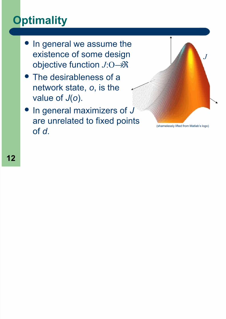
Optimality

In general we assume the

existence of some design

objective function J :O→ℜ

The desirableness of anetwork state, o, is the

value of J (o).

In general maximizers of J

are unrelated to fixed points

of d .(shamelessly lifted from Matlab’s logo)

J



13

Showing convergence with nonlinear programming

(shamelessly lifted from Matlab’s logo)

J α

Left unanswered: where does α come from?



14

Stability

x

y

x

y

Stable, but not attractive

x

y

Attractive, but not stable



15

Lyapunov’s Direct Method

Left unanswered: where does L come from?



16

Analysis models appropriate for dynamical systems

Contraction Mappings – Identifiable unique steady-state – Everywhere convergent, bound for convergence

rate – Lyapunov stable (δ =ε )

Lyapunov function = distance to fixed point – General Convergence Theorem (Bertsekas)

provides convergence for asynchronous timing if contraction mapping under synchronous timing

Standard Interference Function – Forms a pseudo-contraction mapping – Can be applied beyond power control

Markov Chains (Ergodic and Absorbing) – Also useful in game analysis

O1

O2

O3

O4

O5

O6

O7

O8O9

O10

O1 1

O1 1

A(t0)

A(t 1)

A(t 2)

A(t 3)

A(t 4)

A(t 5)

A(t 6)

A(t 7)

A(t8)

A(t 8

)

A(t 9

)



17

Markov Chains

Describes adaptationsas probabilistictransitions betweennetwork states.

– d is nondeterministic Sources of

randomness: – Nondeterministic timing

– Noise

Frequently depicted asa weighted digraph or as a transition matrix



18

General Insights ([Stewart_94])

Probability of occupying a stateafter two iterations. – Form PP.

– Now entry pmn in the mth row and nth column of PP represents the

probability that system is in statean two iterations after being instate am.

Consider Pk . – Then entry pmn in the mth row and nth

column of represents theprobability that system is in statean two iterations after being instate am.



19

Steady-states of Markov chains

May be inaccurate to consider a Markovchain to have a fixed point – Actually ok for absorbing Markov chains

Stationary Distribution – A probability distribution such that π * such that

π *T P =π *T is said to be a stationary distributionfor the Markov chain defined by P.

Limiting distribution – Given initial distribution π

0 and transition matrixP, the limiting distribution is the distribution thatresults from evaluating

0lim T k

k π

→∞P



20

Ergodic Markov Chain

[Stewart_94] states that a Markov chain is ergodic if

it is a Markov chain if it is a) irreducible, b) positive

recurrent , and c) aperiodic .

Easier to identify rule: – For some k Pk has only nonzero entries

(Convergence, steady-state) If ergodic, then chain

has a unique limiting stationary distribution.



21

Absorbing Markov Chains

Absorbing state – Given a Markov chain with transition matrix P, a

state am is said to be an absorbing state if pmm=1.

Absorbing Markov Chain – A Markov chain is said to be an absorbing Markov

chain if it has at least one absorbing state and

from every state in the Markov chain there exists asequence of state transitions with nonzero probability

that leads to an absorbing state. These nonabsorbing

states are called transient states.

a0 a1

a

2 a3 a4 a5



22

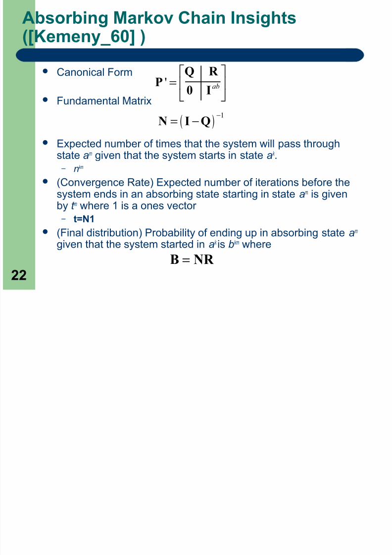
Absorbing Markov Chain Insights([Kemeny_60] )

Canonical Form

Fundamental Matrix

Expected number of times that the system will pass throughstate am given that the system starts in state ak . – nkm

(Convergence Rate) Expected number of iterations before thesystem ends in an absorbing state starting in state am is given

by t m where 1 is a ones vector – t=N1

(Final distribution) Probability of ending up in absorbing state am given that the system started in ak

is bkm where

' ab =

Q R P

0 I

( )1−= −N I Q

=B NR



23

Two-Channel DFS

( f 1, f 1) ( f 1, f 2)

( f 2, f 2)( f 2, f 1)

0.25

0.25

0.25

0.25

0.25

1

1 0.25

0.25

0.25

( f 1, f 1) ( f 1, f 2)

( f 2, f 2)( f 2, f 1)

0.25

0.25

0.25

0.25

0.25

1

1 0.25

0.25

0.25

0.250.250.250.25( f 2, f 2)

0100( f 2, f 1)

0010( f 1, f 2)

0.250.250.250.25( f 1, f 1)

( f 2, f 2)( f 2, f 1)( f 1, f 2)( f 1, f 1)

0.250.250.250.25( f 2, f 2)

0100( f 2, f 1)

0010( f 1, f 2)

0.250.250.250.25( f 1, f 1)

( f 2, f 2)( f 2, f 1)( f 1, f 2)( f 1, f 1)

P =

1.50.5( f 2, f 2)

0.51.5( f 1, f 1)

( f 2, f 2)( f 1, f 1)

1.50.5( f 2, f 2)

0.51.5( f 1, f 1)

( f 2, f 2)( f 1, f 1)

N =0.50.5( f 2, f 2)

0.50.5( f 1, f 1)

( f 2, f 1)( f 1, f 2)

0.50.5( f 2, f 2)

0.50.5( f 1, f 1)

( f 2, f 1)( f 1, f 2)

B =

( )1

1

j j

j

j j

f f u a

f f

−

−

≠= − =

( )

( )

( )

1

, \ 1

j j

j j j j j

f u a

d f f f F f u a−

=

= ∈ = −

Decision Rule

Goal

TimingRandom timer set to go off with probability

p=0.5 at each iteration



24

Procedural Radio Analysis Models



25

Model Steady States



26

Model Convergence



27

Model Stability



28

Using Game Theory to AnalyzeCognitive Radio Networks



29

Modeling Assumptions

Model of <N , A,{u i },{d

i },T >

Adaptations increase player’s goal

Asynchronous myopic repeated game model



30

Nash Equilibrium (Steady-state)

Friend

Foe

Friend Foe

500,500 0,1000

0,01000,0



31

Nash Equilibrium Identification

Exhaustive Search – Time to find all NE can be significant

– Only appropriate for finite action spaces

–

Not every game has an NE

P R S

S

R

P 0, 0

0, 0

0, 0

1, -1

1, -1

1, -1 -1, 1

-1, 1

-1, 1

Paper – Rock – Scissors



32

Nash Equilibrium as a Fixed Point

Best Response function

Synchronous Best Response

Nash Equilibrium as a fixed point

Fixed point theorems can be used toestablish existence of NE (see dissertation)

NE can be solved by implied system of

equations

( ) ( ) ( ){ }ˆ : , ,i i i i i i i i i i i B a b A u b a u a a a A− −= ∈ ≥ ∀ ∈

( ) ( )ˆ ˆii N B a B a∈= ×

( )* *ˆa B a=



33

Significance of NE for CRNs

Why not “if and only if”? – Consider a self-motivated game with a local maximum

and a hill-climbing algorithm. –

For many decision rules, NE do capture all fixed points(see dissertation) Identifies steady-states for all “intelligent” decision rules

with the same goal. Implies a mechanism for policy design while

accommodating differing implementations –

Verify goals result in desired performance – Verify radios act intelligently



34

Pareto efficiency (optimality)

Formal definition: An action vector a* is Pareto

efficient if there exists no other action vector a, such

that every radio’s valuation of the network is at least

as good and at least one radio assigns a higher

valuation Informal definition: An action tuple is Pareto

efficient if some radios must be hurt in order to

improve the payoff of other radios.

Important note – Like design objective function, unrelated to fixed points (NE)

– Inferior to evaluating design objective function (see

dissertation)



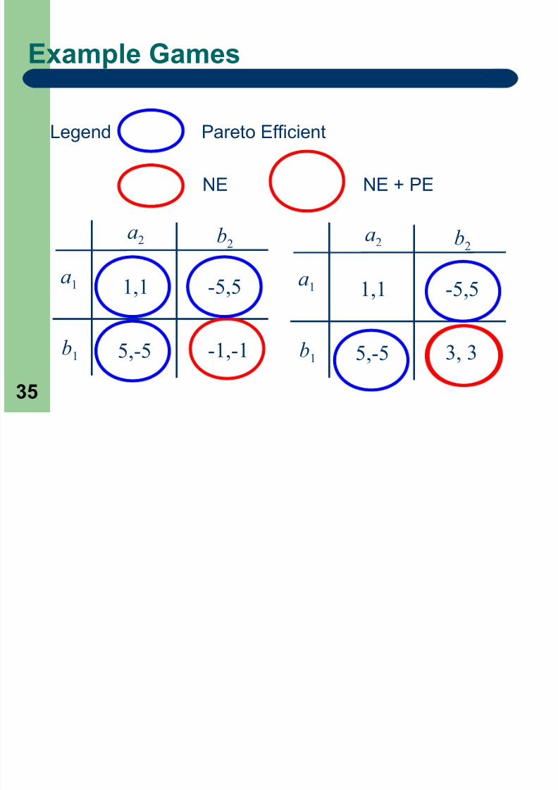
35

Example Games

a1

b1

a2 b2

1,1 -5,5

-1,-15,-5

a1

b1

a2 b2

1,1 -5,5

3, 35,-5

Legend Pareto Efficient

NE NE + PE



36

Paths and Convergence

Path [Monderer_96] – A path in Γ is a sequence γ = (a0, a1,…) such that for every

k ≥ 1 there exists a unique player such that the strategy

combinations (ak-1, ak ) differs in exactly one coordinate.

–

Equivalently, a path is a sequence of unilateral deviations.When discussing paths, we make use of the following

conventions.

– Each element of γ is called a step.

– a0 is referred to as the initial or starting point of γ .

– Assuming γ is finite with m steps, am

is called the terminal point or ending point of γ and say that γ has length m.

Cycle [Voorneveld_96] – A finite path γ = (a0, a1,…,ak ) where ak = a0



37

Improvement Paths

Improvement Path

– A path γ = (a0, a1,…) where for all k ≥ 1, u i (ak )>u

i (ak -

1) where i is the unique deviator at k

Improvement Cycle – An improvement path that is also a cycle

γ 2

γ 1

γ 3

γ 4γ 5γ 6γ 2

γ 1

γ 3

γ 4γ 5γ 6



38

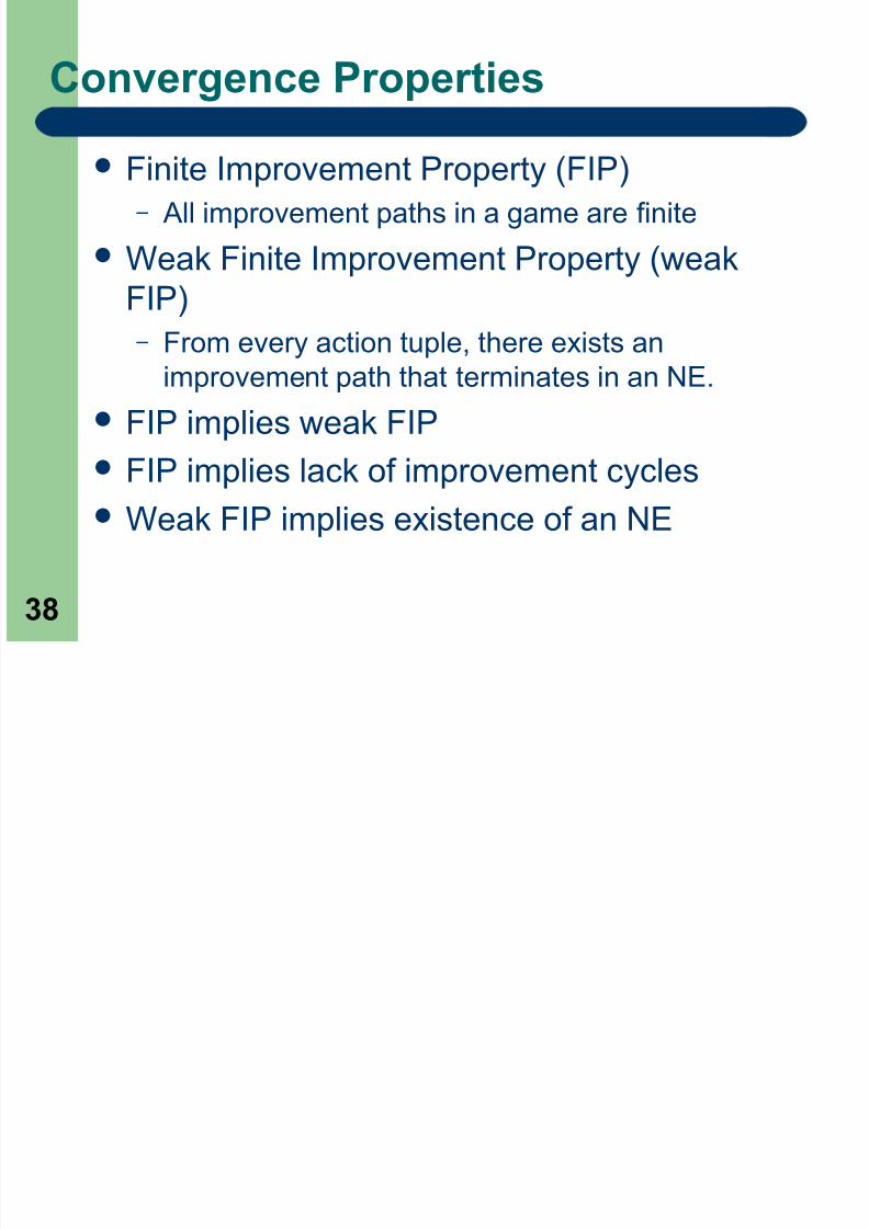
Convergence Properties

Finite Improvement Property (FIP) – All improvement paths in a game are finite

Weak Finite Improvement Property (weak

FIP) – From every action tuple, there exists an

improvement path that terminates in an NE.

FIP implies weak FIP

FIP implies lack of improvement cycles

Weak FIP implies existence of an NE



39

Examples

a

b

A B

1,-1

-1,1

0,2

2,2

Game with FIP

a

b

A B

1,-1 -1,1

1,-1-1,1

C

0,2

1,2

c 2,12,0 2,2

Weak FIP but not FIP



40

Implications of FIP and weak FIP

Unless the game model of a CRN has weak FIP,then no autonomously rational decision rule can beguaranteed to converge from all initial states under random and round-robin timing (Theorem 4.10 indissertation).

If the game model of a CRN has FIP, then ALLautonomously rational decision rules are guaranteedto converge from all initial states under random andround-robin timing.

– And asynchronous timings, but not immediate fromdefinition

More insights possible by considering more refinedclasses of decision rules and timings



41

Decision Rules

Ab bi M k Ch i d



42

Absorbing Markov Chains andImprovement Paths

Sources of randomness – Timing (Random, Asynchronous) – Decision rule (random decision rule) – Corrupted observations (not assumed yet)

An NE is an absorbing state for autonomously

rational decision rules. Weak FIP implies that the game is an absorbing

Markov chain as long as the NE terminatingimprovement path always has a nonzero probabilityof being implemented.

This then allows us to characterize – convergence rate, – probability of ending up in a particular NE, – expected number of times a particular transient state will be

visited

Connecting Marko models



43

Connecting Markov models,improvement paths, and decision rules

Suppose we need the path γ = (a0, a1,…am) for convergence byweak FIP.

Must get right sequence of players and right sequence of adaptations.

Friedman Random Better Response

– Random or Asynchronous Every sequence of players have a chance to occur Random decision rule means that all improvements have a chance to

be chosen

– Synchronous not guaranteed

My random better response (chance of choosing same action) – Because of chance to choose same action, every sequence of

players can result from every decision timing.

– Because of random choice, every improvement path has a chanceof occurring



44

Convergence Results (Finite Games)

If a decision rule converges under round-robin, random, or synchronous timing, then it also converges under asynchronoustiming.

Random better responses converge for the most decision timingsand the most surveyed game conditions. – Implies that non-deterministic procedural cognitive radio

implementations are a good approach if you don’t know much aboutthe network.



45

Impact of Noise

Noise impacts the mapping from actions tooutcomes, f : A→O

Same action tuple can lead to different outcomes

Most noise encountered in wireless systems istheoretically unbounded.

Implies that every outcome has a nonzero chanceof being observed for a particular action tuple.

Some outcomes are more likely to be observedthan others (and some outcomes may have a verysmall chance of occurring)



46

DFS Example

Consider a radio observing the spectralenergy across the bands defined by the set C where each radio k is choosing its band of operation f k .

Noiseless observation of channel c k

Noisy observation If radio is attempting to minimize inband

interference, then noise can lead a radio tobelieve that a band has lower or higher

interference than it does

( ) ( ),i k ki k k k

k N

o c g p c f θ ∈

= ∑( ) ( ) ( ), ,i k ki k k k i k

k N

o c g p c f n c t θ

∈

= +∑%



47

Trembling Hand (“Noise” in Games)

Assumes players have a nonzero chance of making an error implementing their action. – Who has not accidentally handed over the wrong

amount of cash at a restaurant?

– Who has not accidentally written a “tpyo”?

Related to errors in observation as erroneous

observations cause errors in implementation

(from an outside observer’s perspective).



48

Noisy decision rules

Noisy utility ( ) ( ) ( ), ,i i iu a t u a n a t = +%

Trembling

Hand

Observation

Errors



49

Implications of noise

For random timing, [Friedman] shows game withnoisy random better response is an ergodic Markovchain.

Likewise other observation based noisy decisionrules are ergodic Markov chains

– Unbounded noise implies chance of adapting (or notadapting) to any action – If coupled with random, synchronous, or asynchronous

timings, then CRNs with corrupted observation can bemodeled as ergodic Makov chains.

– Not so for round-robin (violates aperiodicity)

Somewhat disappointing – No real steady-state (though unique limiting stationary

distribution)



50

DFS Example with three access points

3 access nodes, 3 channels, attempting to operate inband with least spectral energy.

Constant power

Link gain matrix

Noiseless observations

Random timing

12

3



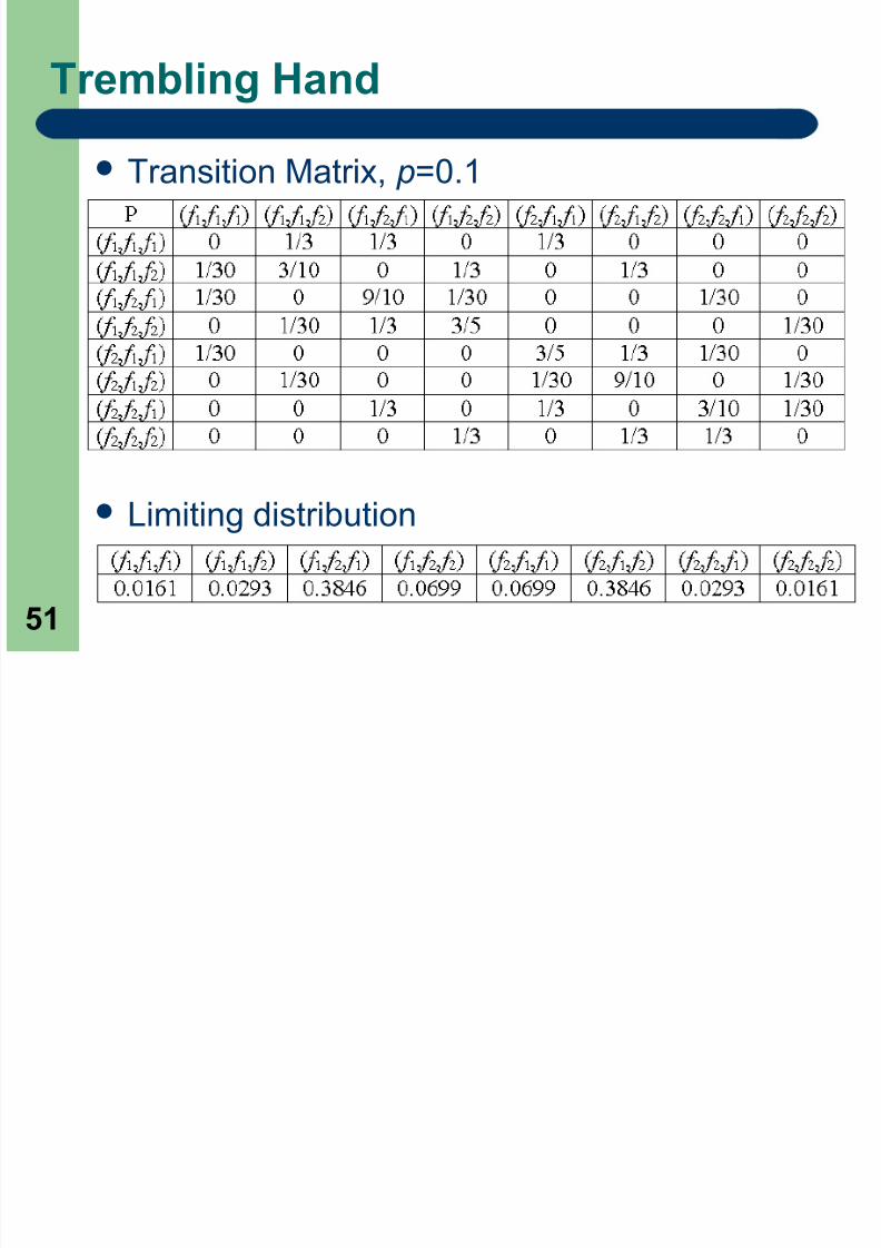
51

Trembling Hand

Transition Matrix, p=0.1

Limiting distribution



52

Noisy Best Response

Transition Matrix, (0,1) Gaussian Noise

Limiting stationary distributions



53

Comment on Noise and Observations

Cardinality of goals makes a difference for cognitiveradios – Probability of making an error is a function of the difference

in utilities – With ordinal preferences, utility functions are just useful

fictions Might as well assume a trembling hand

Unboundedness of noise implies that no state can beabsorbing

NE retains significant predictive power – While CRN is an ergodic Markov chain, NE (and the

adjacent states) remain most likely states to visit – Stronger prediction with less noise – Also stronger when network has a Lyapunov function – Exception - elusive equilibria ([Hicks_04])



54

Summary

Skipped over a lot of stuff in the dissertation Given a set of goals, an NE is a fixed point for all radios with

those goals for all autonomously rational decision processes Traditional engineering analysis techniques can be applied in a

game theoretic setting

– Markov chains to improvement paths Network must have weak FIP for autonomously rational radios

to converge – Weak FIP implies existence of absorbing Markov chain for many

decision rules/timings

In practical system, network has a theoretically nonzero chanceof visiting every possible state (ergodicity), but does haveunique limiting stationary distribution – Specific distribution function of decision rules, goals



55

Shortcomings

Steady-states – Need not be optimal

Could enforce desired equilibria Doesn’t generally scale well

– Identification in finite games is painful Game convergence

– Only looked at finite games – Arguably all DSP controlled radios have a finite action space, but

to a casual observer, action space may appear infinite – How to identify when a game has FIP/weak FIP without exhaustive

search? – Would like to be able to apply Zangwill’s for infinite action spaces

Noise/Stability – Characterizing state distribution not exactly the same as stability – Where do the functions for applying Zangwill’s Theorem and

Lyapunov’s Direct Method come from? Solution: potential games and the interference reducing

network design framework (next week)



Questions?

analysis aug30 edit1

Documents