ANALYSIS OF GAS CARRY-UNDER IN GAS-LIQUID CYLINDRICAL CYCLONES

by

S. K. Marti, F. M. Erdal, O. Shoham, S. A. ShiraziThe University of TulsaandG. E. KoubaChevron Petroleum Technology Company

ABSTRACT

Existing theories for cyclone separators, developed for liquid-liquid, liquid-solid and gas-solidflows, can handle low concentrations of the dispersed phase. These models are not appropriatefor gas-liquid cylindrical cyclone (GLCC) separators over a full range of gas fractions, becausethe flow dynamics and phase distribution are not limited to dispersed flow. Indeed, in the gas-liquid cyclone several flow patterns may occur, including churn, mist, annular, dispersed bubblesand separated flows. Furthermore, several of these flow patterns may occur in the cyclone underthe same inlet flow conditions.

This paper presents a first attempt to develop a mechanistic model to predict gas carry-under inGLCC separators. The model predicts the gas-liquid interface near the GLCC inlet as a functionof the radial distribution of the tangential velocity. The interface defines the starting location forthe bubble trajectory analysis, which enables determination of gas carry-under and separationefficiency for the GLCC. The decay of the tangential velocity in the axial flow direction isincorporated. Also presented are preliminary CFD simulation results obtained from a commercialpackage (CFX). The proposed study is a part of a comprehensive model for a proper design ofindustrial GLCC separators.

2

INTRODUCTION

Cyclone separators have been in existence for at least 150 years, yet the use of cyclones in the oilfield is a fairly recent phenomenon. The high performance and relatively small size of cycloneseparators makes them an extremely attractive alternative technology for offshore applications.The short fluid residence times of cyclones translate into much smaller equipment thanconventional gravity based separation facilities. This can be critical on offshore platforms, whereweight and space requirements have a significant multiplier effect on the overall cost of theseparation facilities. Liquid-liquid and liquid-solid hydrocyclone technology have grown rapidlyover the last decade, but full range compact gas-liquid cyclone technology is only just beginningto emerge.

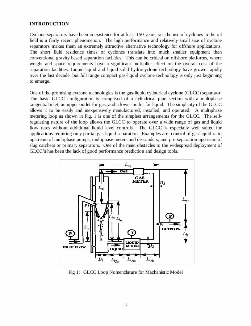
One of the promising cyclone technologies is the gas-liquid cylindrical cyclone (GLCC) separator.The basic GLCC configuration is comprised of a cylindrical pipe section with a multiphasetangential inlet, an upper outlet for gas, and a lower outlet for liquid. The simplicity of the GLCCallows it to be easily and inexpensively manufactured, installed, and operated. A multiphasemetering loop as shown in Fig. 1 is one of the simplest arrangements for the GLCC. The self-regulating nature of the loop allows the GLCC to operate over a wide range of gas and liquidflow rates without additional liquid level controls. The GLCC is especially well suited forapplications requiring only partial gas-liquid separation. Examples are: control of gas-liquid ratioupstream of multiphase pumps, multiphase meters and de-sanders, and pre-separation upstream ofslug catchers or primary separators. One of the main obstacles to the widespread deployment ofGLCC’s has been the lack of good performance prediction and design tools.

Lg2

Lg1

LlwLin

Ll1

P1

Ll2a Ll2m Ll2b

D2

D1

Ll3

P2

Lg3

D3

Fig 1: GLCC Loop Nomenclature for Mechanistic Model

3

The state-of-the-art in predicting cyclone performance has in the past revolved solely aroundcomputational fluid dynamic modeling of the flow field and the trajectories of discreet particles ofthe dispersed phase. While well suited for local modeling of single phase and dispersed two-phaseflows, present CFD models are unable to handle some of the complex flow regimes observed inthe GLCC, in particular, slug and churn flows. Furthermore, CFD models of large system, e.g.,the multiphase metering loop shown in Fig. 1, are too unwieldy to be practical for designpurposes.

Mechanistic modeling offers a practical approach to GLCC design and performance predictionthat is complementary to CFD work. Mechanistic models make simplifying assumptions whilestill capturing the fundamental physics of the problem, consequently, they are not as detailed,rigorous, or accurate as the CFD models. Advantages of mechanistic models include speed,ability to model entire system, run on PC and, therefore, are more accessible to engineers as adesign tool than CFD models. Our approach is to develop fundamental mechanistic models andverify and refine them with experimental data and CFD predictions.

Most of the studies published on cyclone separators have been focused on liquid-liquid, liquid-solid and gas-solid flows. Very few studies on gas-liquid flows in the GLCC have been reported.Recently, Kouba et al. (1995) and Arpandi et al. (1995) developed and discussed mechanisticmodels that predict liquid carry-over with the gas stream. A comprehensive review of theliterature on gas-liquid flow in GLCC’s and related topics is also given by them. Kurokawa andOhtaki (1995) conducted an experimental study on the characteristics of gas-liquid swirling flowand the gas separation efficiency of a spiral type cyclone separator. A honeycomb type swirlbreaker is utilized to improve the gas separation efficiency.

Two studies for fluid system other than gas-liquid are relevant to the determination of separationefficiency in a GLCC. Wolbert et al. (1995) utilized droplet trajectory analysis for the estimationof separation efficiency for liquid-liquid (oil-water) flow in hydrocyclones. Trajectories werecharacterized through a differential equation combining models for the three velocitydistributions, namely, axial radial and tangential, and the settling velocity defined by Stoke’s law.A characteristic droplet diameter, d100, was defined which corresponds to the smallest dropletdiameter that will be separated with a 100% efficiency. Kutepov et al. (1978) conducted anexperimental and theoretical investigation on the separation efficiency of hydrocyclones for solid-liquid separation. A method for calculating the amounts of solid phase carried with the liquidphase in both the clear and thickened products of separation was developed based on stochastictheory of separation processes.

The literature reveals a lack of both experimental studies and predictive methods for gas carry-under phenomenon in GLCC’s. The aim of this work is to lay the foundation for characterizinggas carry-under and determining separation efficiency.

Three mechanisms have been identified as possible ways that gas is carried under with liquid: 1)the trajectory of individual bubbles is too shallow for small bubbles to escape to the gas core, 2)gas core instability results in the gas core filament whipping helically and occasionally breaking

4

off, and 3) a bubble swarm instability occurs with a sudden increase of liquid rate producing acloud of bubbles that are unable to migrate to the gas core. This study addresses the firstmechanism, i.e., the trajectory of small individual bubbles.

MECHANISTIC MODELING

The trajectory of an individual bubble is determined from a force balance on the bubble. This firstrequires an approximation of the velocity field in the GLCC. The axial release point for thebubble is determined from the location of the gas vortex. The d100 bubble is the smallest bubblewhose trajectory will just allow all bubbles of this size to be captured and flow upwards with thegas core. The bubble capture efficiency is the percentage of bubbles of a certain size that arecaptured in the gas core. In order to determine an overall separation efficiency with respect togas carry-under, the bubble size distribution and total amount of entrained gas would have to beknown. Although beyond the scope of the present paper, the overall separation efficiency is thedesired outcome of this work.

The model for gas carry-under and determination of separation efficiency is developed throughbubble trajectory analysis, by extending the studies of Kouba et al. (1994) and Arpandi et al.(1995), and using a similar approach presented by Wolbert et al. (1995) for liquid-liquid flow inhydrocyclones.

A schematics of the physical system is given in Fig. 1. The GLCC is shown in a multiphase flowmetering loop configuration. The gas and liquid mixture is introduced into the GLCC through aninclined tangential inlet. The inclined section promotes stratification and pre-separation of thephases, which then enter tangentially into the GLCC through a slot. The flow from the inlet slotgenerates a swirl near the inlet of the GLCC. Due to the centrifugal forces, the liquid phase ispushed to the wall while the gas phase moves to the center. The gas phase exits from the top intothe gas leg, and the liquid phase exits from the bottom through the liquid exit. A thin gas corefilament is created below the vortex by the smaller bubbles separated below the vortex region. Inthis configuration the gas and the liquid phases are metered utilizing conventional flow metersbefore being recombined at the exit of the loop. The figure includes all the dimensions of theGLCC and the different sections of the flow loop.

Preliminary CalculationsPrior to bubble trajectory analysis, it is essential to determine the distribution of the gas and theliquid in the GLCC. This includes the equilibrium liquid level and the gas-liquid interface shapeand location. These models were presented in detail by Arpandi et al. (1995) and are summarizedbriefly below for completeness.

Equilibrium Liquid Level: The equilibrium liquid level simply corresponds to the pressure drop inthe GLCC as measured by an external sight gauge (glass level indicator). Because the frictionallosses are low in the GLCC, the equilibrium liquid level indicates the amount of liquid in theGLCC.

5

The equilibrium liquid level is determined from a simple pressure balance between the inlet (P1)and the outlet (P2) of the flow loop, for the gas leg and the liquid leg. This simple model neglectsany hydrodynamic interaction between the phases. Equating the pressure drops along the liquidand gas legs one can solve explicitly for the equilibrium liquid level, as follows:

LgL g L L L

gv f

D

ll g l l g in g g

l gl l l

1

3 1 3

1

2

1

12

=− + − + −

− −

Φ Φ ρ ρ

ρ ρρ

( )

( )

(1)

where Φ l and Φ g are the frictional pressure losses in the liquid and gas sections, given as:

Φ ll i i i

ii i

j

m

i

n

l

f L vD

K v= +

==∑∑ρ

2

22

12

(2)

Φ gg i i i

ii i

j

m

i

n

g

f L vD

K v= +

==∑∑ρ

2

22

11(3)

The terms inside the parentheses of Eqs. (2) and (3) represent the frictional losses in the differentpipe segments of the flow loop and the losses in the piping fittings, respectively.

Gas-Liquid Interface: The main assumption for this model is that the interface occurs due to aforced vortex caused by the tangential inlet flow into the GLCC. The occurrence of a forcedvortex in a GLCC was substantiated by the experimental measurements of Millington and Thew(1987). The tangential velocity distribution in the vortex is given by:

( )v r vrRt t is

s

n

=

(4)

where n = 1 for forced vortex, i.e., solid body rotation, n = -1 for free vortex, and -1<n<1 for acombination vortex. In this study it is assumed that the tangential flow from the inlet generates aforced vortex in the GLCC (n = 1). The tangential velocity from the inlet slot, vt is , is determinedfrom the liquid velocity at the inclined inlet section vlin , corrected for the slot area reduction and

for the inlet section inclination angle, α (α = 270), as follows:

( )v vAAt is l

in

isin

= cos α . (5)

where the liquid velocity at the inlet section, vlin , is calculated from the Taitel and Dukler (1976)

model.

6

The centrifugal force gives rise to a radial pressure difference across the vortex, namely, betweenthe gas-liquid interface and the GLCC wall, as follows:

( )( )[ ]

∆P rv r

rdr

l t

R

r

s

= ∫ρ 2

. (6)

The radial pressure difference is balanced by the hydrostatic pressure difference between theliquid and the gas phases in the vortex. Thus, the axial location of the interface at any radialposition, r, can be obtained from the equation below:

( ) ( )( )z r

P r

g l g

=−

∆ρ ρ

. (7)

The interface location z(r) can be used to calculate the total liquid volume displaced by the gasvortex and gas core filament, yielding:

( )V rz r dr R L zgR

R

c l t

c

s

w= + −∫2 2π π( ) (8)

where Rc is the gas core filament radius and zt = z(Rc) is the length of the vortex. The highestpoint of the liquid vortex, where the interface touches the GLCC wall (vortex crown), can becalculated assuming the total gas volume is submerged into the volume of liquid resulting fromthe equilibrium liquid level calculation, as follows:

L LVAl l

g

sw

= +1

(9)

Bubble TrajectoryThe starting axial location for the bubble trajectory is the bottom of the vortex. In the vortexregion the large bubbles are captured easily. At the bottom of the vortex the remaining smallbubbles are assumed to be homogeneously distributed. Below the vortex, the bubbles moveradially towards the GLCC centerline due to centripetal forces, and axially downward due to dragforces from the axial flow of the liquid phase. If a bubble travels sufficiently radially inward, itwill merge with the gas core and will be carried upward by the gas stream. If, however, theradial distance traveled by the bubble is insufficient, it will be carried under by the liquid streaminto the liquid leg exit.

Fig. 2 shows schematically the bubble trajectory model. The bubble is shown at time t and at timet + ∆t. The bubble moves radially at a velocity vr(r) and axially at the surrounding fluid

7

velocity, vz. The buoyancy force and slippage acting on the bubble in the z direction are neglected.As a result the bubble will move farther in the radial direction, yielding an earlier gas carry-underprediction, which is conservative from the design point of view. As a first approximation, thevelocity profile in the z direction is assumed to be uniform, namely, vz(r) = vz. The totalvelocity of the bubble is vb(r), as shown in the figure. During the time interval, ∆t, the bubblemoves dr = vr(r)∆t and dz = vz ∆t in the radial and axial directions, respectively. Equating thetime period for the radial and axial movements of the bubble, and solving for the axial distanceyields the equation governing the bubble trajectory:

dz vdr

v rzr

=( )

(10)

θ

Fig 2: Schematics of Bubble Trajectory

The velocity distribution in the radial direction can be determined from a force balance on thebubble. The forces acting on the bubble in the radial direction are the centripetal (centrifugal andbuoyancy), turbulent and drag forces.

Assuming local equilibrium at any radial location along the trajectory path traveled by the bubble,a force balance on the bubble yields:

F F Frd rc rt= ± (11)

r

z

v(r)

vb

drdz

Interface

Trajectory

vz

8

The centripetal force, Frc, is equal to the sum of the centrifugal force and buoyancy force actingon the bubble, namely:

( ) ( )F

v rr

Rrc l gt

b= − −ρ ρ π2

343

. (12)

The total drag force on the bubble, Fd, is determined from:

( )F

C v r Rd

d l b b= ρ π2 2

2(13)

and the radial component of the drag force is:

( ) ( )F F F

vv

C v r v r Rrd d d

r

b

d l b r b= = =cosθ ρ π 2

2(14)

The total turbulent force acting on the bubble is estimated in the same method proposed by Levich(1962), as follows:

( )Fv r R

tl b b= ρ π'

2 2

2(15)

where ( )v rb' is the fluctuating component of the bubble velocity calculated by:

( )v r v fb b l' 2 2= (16)

where fl is the friction factor. Substituting Eq. (16) into (15) and solving for the radial componentof the turbulent force yields:

Ff v r v r R

rtl r b b=

ρ π( ) ( ) 2

2(17)

Equating the radial forces from Eqs. (12), (14) and (17), as implied in Eq. (11), the radial velocitydistribution can be solved as:

( ) ( )( )v r

v rr

dC f v rr

l g

l

t b

d l b

=−

±43

12ρ ρρ ( )

. (18)

9

The value of the drag coefficient, Cd, is calculated with a modified correlation developed byTurton and Levenspiel (1986) and presented by Karamanev and Nikolov (1992) as:

( )( )[ ]

( ) ( )( )C rR r

R r R rd

e

e e

=+

++ −

24 1 0173 0 4131 16 300

0 657

1 09

. .,

.

.

for Re ≤ 400 (19a)

It was found out that the original correlation given in Eq. (19a) is valid in the range Re<400. Anew correlation is developed for the higher Reynolds number range, based on the data ofHaberman and Morton (1953), reported by Perry (1963), as follows:

C r R r R rd e e( ) ( ) ( ) .= − + +− −10 10 012227 2 3

for 400 ≤ Re ≤ 5000 (19b)

C rd ( ) .= 2 4 for Re ≥ 5000 (19c)

The Reynolds number is:

( ) ( )R r

v r de

l b b

l

=ρ

µ . (20)

The radial velocity distribution given by Eq. (18) can be substituted into Eq. (10). Integration ofEq. (10) yields the bubble trajectory z(r), as follows:

( ) ( )z rv

v rdrz

rR

r

s

= ∫ . (21)

Stepping through r, from r = Rs to r = Rc maps out the entire trajectory of the bubble.

Tangential Velocity DecayThe maximum tangential velocity occurs at the inlet slot of the GLCC. As the flow swirls aroundand moves downwards, the tangential velocity reduces due to viscous dissipation. Thisphenomenon must be predicted and accounted for as it reduces the separation efficiency of theGLCC.

The analysis is carried out on the swirling flow in a control volume bounded by the wall, asshown in Fig. 3. A force balance on the control volume in the θ direction yields:

F dA dV aw l lθ θτ β ρ= − =cos (22)

10

where β is the angle of the tangential velocity vector with respect to the horizontal. The wallshear stress τw is given by:

τρ

w ll tfv

=2

8(23)

Fig 3: Control Volume for Tangential Velocity Decay Analysis

Substituting for the shear stress into Eq. (22), dividing through by ρl, and assuming that the

characteristic length dVdA

l , is proportional to the radial increment dr, namely, dVdA

kdrl = , results:

− =fv

kdralt2

8cosβ θ (24)

The acceleration is:

a vdvrdθ θ

θ

θ= (25)

Substituting Eq. (25) into Eq. (24) yields:

vdvrd

fvkdrl

tθ

θ

θ β= −2

8cos (26)

dr

rdθ

dz β

11

Dividing Eq. (26) by vθ2 , and recalling that

vvt

θ β= cos results in:

dvv

fkdr

rdlθ

θ β θ= −8 cos

(27)

Substituting rddz

θ β=tan

and approximating dzkdr

LD2

= Eq. (27) becomes:

dvv

f LD

lθ

θ β= −4sin

(28)

As an example (used later in the CFD analysis), for v t is= 10 ft/s and vz = 0.5 ft/s, the angle of the

tangential velocity vector is β = 30. Also, the smooth pipe friction factor for fully developed

turbulent flow is fl ≈ 0.06. For this case the tangential velocity decay is dvv

LD

θ

θ= 56%. . This

appears to be in a reasonable agreement with the experimental data of Hargreaves and Silvester(1990) reported by Wolbert et al. (1995), and as shown later is in favorable agreement with thepresent study CFD calculations.

Separation EfficiencyA schematics of the method for the determination of the separation efficiency is shown in Fig. 4.As shown, the d100 bubble is the minimum bubble diameter which if released at the pipe wall (r= Rs) below the vortex will move sufficiently radially to be captured by the gas core just beforethe liquid outlet at the bottom of the GLCC. All bubbles of equal or larger diameter than the d100

bubble will be captured with an efficiency of 100%. However, smaller diameter bubbles, db< d100,can be captured by the gas core only if they are released at a different radial location (Rc<r<Rs)and not at the pipe wall. For this case, however, the probability of capturing the smaller bubble isless than that of the d100 bubble, resulting in lower efficiency for this bubble size. For the exampleshown in Fig. 4, the smaller bubble is released at the radial location re. This bubble will becaptured at any radial release location r<re, resulting in an effective area for capture ofπre

2 . Theseparation efficiency for this bubble is based on the ratio of the effective area for capture to thetotal cross sectional area, namely:

ErR

rR

e

s

e

s

(%) = =

ππ

2

2

2

(29)

12

Fig 4: Schematics of Separation Efficiency Analysis

RESULTS AND DISCUSSION

Mechanistic ModelThe results obtained from the proposed model are plotted in Figs. 5-10. The results are predictedfor a GLCC metering loop, as shown schematically in Fig. 1, which was utilized in this study.The GLCC is 3 in. in diameter, 7.6 ft high (3.4 ft and 4.2 ft above and below the inlet,respectively). The inlet is a 3 ft long 2 in. pipe section inclined at 270 below the horizontal. Thearea of the inlet slot is 2.5 in.2. The gas and liquid phases are metered with a gas vortex sheddingmeter and a Micromotion meter, respectively, before being recombined at the loop exit. Thesystem is operated with air-water at atmospheric conditions.

Fig. 5 shows the effect of the operational flow rates (expressed in terms of the superficialvelocities of the gas and liquid phases in the GLCC) on d100. As can be seen in the figure, the gasvelocity does not have a significant effect on the d100 at low liquid velocities. At high liquidvelocities, however, there is an increase in d100 with increasing gas velocities. Also, as the liquidflow rate increases, the d100 increases significantly. Note that the size of the bubbles is below 0.1mm, as the larger bubbles are captured upstream in the vortex region.

Lt

zt

Llw

InletFlow

Liquid

Gas

Rsre

d100

13

0

0.02

0.04

0.06

0.08

0.1

0 10 20 30 40

v sg (ft/s)

d10

0 (

mm

)

Vsl = 0.05 ft/s

Vsl = 0.1 ft/s

Vsl = 0.5 ft/s

Fig 5: Variation of d100 for a 3” GLCC Operated with Air-Water at Atmospheric Conditions

0

1

2

3

4

5

6

0 5 10 15 20 25

v t is (ft/s)

zt

Vsl = 0.05 ft/s

Vsl = 0.1 ft/s

Vsl = 0.5 ft/s

Fig 6: Effect of Tangential Velocity on Vortex Length for a 3” GLCC Operated with Air-Waterat Atmospheric Conditions

14

The effect of inlet slot tangential velocity on the length of the vortex, zt, can be seen in Fig. 6. Theresult of increasing the tangential velocity is an increase in vortex length and a reduction in axialdistance available for the bubble trajectory, which can cause a reduction in the separationefficiency.

Fig. 7 demonstrates the effect of the ratio of inlet slot tangential velocity to axial velocity, vv

tis

z

,

on d100. This ratio is significant because it determines the radial and axial distances traveled by thebubble, which in turn affect the optimum diameter and length of the GLCC. As can be seen, the

d100 is high for low values of vv

tis

z

, but decreases sharply as the ratio is increased, above 100. For

this region, due to high tangential velocity causing higher centripetal forces, and low axialvelocity resulting in larger residence time, the separation efficiency is high as manifested by thesmall value of d100.

0

0.02

0.04

0.06

0.08

0.1

0 50 100 150 200 250

v t is /v z

d10

0 (

mm

)

Vsl = 0.05 ft/s

Vsl = 0.1 ft/s

Vsl = 0.5 ft/s

Fig 7: Effect of the Ratio of Tangential Velocity to Axial Velocity on d100 for a 3” GLCCOperated with Air-Water at Atmospheric Conditions

The effect of the tangential velocity decay on d100 is demonstrated in Fig. 8. As can be seen, forincreasing percent decay factors, the d100 increases linearly indicating lower separation efficiency.This is more pronounced for higher operational liquid velocity conditions given by the upper line.For our study, as indicated before, the theoretical analysis predicts a decay factor of 5.6%.

15

0

0.04

0.08

0.12

0.16

0.2

0 2 4 6 8 10

% Decay per L/D

d100

(m

m)

Vsl = 0.5 ft/s, Vsg = 5 ft/s

Vsl = 0.1 ft/s, Vsg = 10 ft/s

Fig 8: Effect of Decay on d100 for a 3” GLCC Operated with Air-Water at AtmosphericConditions

Fig. 9 shows the bubble trajectories for a 0.4 mm bubble released at different radial locationsbelow the vortex region for one set of operating conditions. If the bubble is released at theGLCC wall, Ro = Rs, it travels an axial distance Lt = 2.7 ft. As the initial radial location of thebubble is decreased, r<Rs, the bubble requires less axial distance to be captured. For example, Lt

= 1.2 ft when the bubble starts at a distance of R0 = 0.25Rs from the centerline. The effect ofturbulence on these trajectories was examined using Eq. 18 with the positive and negative signs inthe turbulence term to represent the worst case scenarios. This analysis indicated that even forthese extreme cases, turbulence does not affect the trajectory much and can be neglected.

The most significant results of the model is presented in Fig. 10. The separation efficiency E(%)is plotted as a function of the bubble diameter for one set of operating conditions, for 0%, 3%and 7% decay factors. The bubble diameters for which the separation efficiency is 100% is thed100 bubbles. As expected, larger d100 values (lower separation efficiencies) are obtained with thehigher % decay factors. For bubbles with smaller diameters than d100, the separation efficiencydrops exponentially. Note that similar plots must be generated for different operational (flowrates) conditions.

16

-3

-2.5

-2

-1.5

-1

-0.5

0

0 0.02 0.04 0.06 0.08 0.1 0.12

Radial distance from wall, r (ft)

Leng

th, L

(ft)

Ro = RsRo = 0.9RsRo = 0.75RsRo = 0.5RsRo = 0.25Rs

Vsl = 0.5 ft/sVsg = 5 ft/sP = 0 Psigdb = 0.4 mm

Operational Conditions :

Radial Locationof Bubble Release:

Fig 9: Bubble Trajectories for a 0.4mm Bubble Released at Different Radial Locations in a 3”GLCC Operated with Air-Water at Atmospheric Conditions

0

20

40

60

80

100

0 0.02 0.04 0.06 0.08 0.1 0.12

d (mm)

% E

ffici

ency

No Decay3% Decay7% Decay

Fig 10: Separation Efficiency for Various Decay Factors for a 3” GLCC Operated with Air-Water at Atmospheric Conditions

17

CFD SimulationCFD simulations were undertaken in this study to support the mechanistic model by addressingthe following unresolved questions: 1) Does a forced vortex correctly describe the tangentialvelocity profile at large axial distances from the inlet? 2) Does the bubble have to migrate all theway to the gas core in order to be captured? 3) How should the GLCC geometry be optimizedwith respect to slot dimensions, GLCC diameter and length? This can be initially studied bylooking at the effect of tangential and the axial velocities and their ratio, v t is

/vz. 4) Is the effect ofturbulence predicted correctly by the mechanistic model? 5) Can CFD simulation give any insightinto the instability of the gas core? A commercially available computational fluid dynamic (CFD)code called CFX (previously CFDS-FLOW3D) was utilized in order to study and betterunderstand the complex flow behavior in the GLCC configuration, and attempt to answer theabove questions.

To evaluate the accuracy of the flow field simulation, the predictions from the CFD code werecompared to experimental data (Farchi, 1985). The experimental data were carried out in a short186 mm ID GLCC (L/D ≈ 2) operating with air and water at atmospheric conditions. Acomparison of the predicted tangential velocity profiles using a 3-D simulation showed very goodagreement with experimental data. Also, an axisymmetric (2-D) simulation of flow in the GLCCwas carried out that likewise showed very good agreement with the experimental data. Fig. 11,for example, shows a comparison between the simulation results and the experimental dataobtained at three different probe locations below the inlet: Probe-1 is located just below the inlet,and Probe-2 and 3 are located 100 and 200 mm below the inlet, respectively.

-0.5

0

0.5

1

1.5

2

2.5

3

0.000 0.012 0.024 0.036 0.048 0.060 0.072 0.083

r (m)

vt( m

/s)

CFX Prediction Probe-1CFX Prediction Probe-2CFX Prediction Probe-3Data Probe-1Data Probe-2Data Probe-3

Fig 11: Tangential Velocity Prediction vs. Data (Farchi, 1985), ml = 2.66 kg/s, mg = 0.002 kg/s

18

Following the verification of the simulations, flow predictions were carried out for the 3 in. GLCCdescribed above. The simulations show that the flow in the GLCC is very complex and includesthree velocity components: the tangential velocity vt, the axial velocity vz, and the radial velocityvr. The highest tangential velocity, vt, is observed at the inlet, as shown in Fig. 12. The hightangential velocity dissipates quickly in the inlet region, resulting in a combined vortex, notpredicted previously. The dissipation continues in the axial direction towards the outlet, similar tothe trend shown in Fig. 11. However, this tangential velocity decay is not as drastic as the oneobserved in the inlet region, and within an axial distance of L/D ≈ 1 the profile becomes that of aforced vortex. Decay of the tangential velocity below the inlet region for the 3 in. GLCC isshown in Fig. 12, using an axisymmetric simulation. The tangential velocity profiles, as a functionof the radial direction, in different axial locations (approximately 0,3,6,9,12, and 24 inches belowthe inlet) are shown. Note that for this case, near the center of the cylinder, the tangentialvelocity is nearly a constant, up to about 12 inches below the inlet. Eventually, the viscousdissipation (boundary layer effects) influences the core region, as shown in Fig. 12, at the axiallocation of 24 inches below the inlet. Furthermore, considering the dissipation away from the inlet

region (L/D>1) results in an approximately 7 6%.LD

decay, which compares favorably with the

56%.LD

decay predicted by the mechanistic model.

Location BelowInlet (inches)

0

0.1

0.2

0.3

0.4

0.5

0.6

0.7

0.8

0.9

1

0.00 0.01 0.02 0.03

r (m)

v t /

vt i

s

24 129 63 0

Fig 12: Tangential Velocity Distribution in 3 inch GLCC, vz = 0.5 ft/s, vtis = 10 ft/s

19

Fig. 13 shows the velocity vectors in a plane in front of the inlet. Secondary upward (axial) flowis observed in center region of the GLCC, while the main axial flow goes downward with theswirl near the wall region. The magnitude of this secondary upward flow is low as compared tothe main tangential flow, but the average axial flow is downward. This secondary flow alsodecays in the axial direction from the inlet toward the outlet, depending on the magnitude of theaverage axial flow velocity. Recall that in the mechanistic model a flat profile is assumed for theaxial velocity, as an approximation. This makes the mechanistic model predictions conservativefor gas carry-under.

Fig 13: Velocity Vectors in a Plane in Front of the Inlet

The axisymmetric flow velocity predictions were used to study the sensitivity of flow behaviorfor different ratios of the inlet tangential velocity, v t is

, to the average axial velocity, vz. Thesesimulations showed that the ratio of inlet tangential velocity to the average axial velocity ( v t is

/vz)has an important effect on hydrodynamic flow behavior in the GLCC. High v t is

/ vz ratio indicatesa strong rotational flow that enhances separation, while a low v t is

/ vz ratio causes a strong decayof the tangential velocity in downward direction and causes gas carry-under.

The v t is/ vz ratio has also a great affect on the capture radius. The region between the secondary

upward flow and the main downward flow (zero axial velocity) is referred to as the captureradius, Rcap, as depicted in Fig. 14. In this region, the gas bubbles are captured and separated,and move upward towards the gas leg. This results in a much larger capture radius than the gas

20

core radius used in the mechanistic model. This will be further investigated and incorporated inthe mechanistic model in the future.

Rcap

Fig 14: Definition of Capture Radius (Rcap)

Location Below Inlet

0

0.1

0.2

0.3

0.4

0.5

0.6

0.7

1 10 100 1000v t is /v z

Rca

p/r

6 inches

12 inches

Fig 15: Variation of Capture Radius with vtis/vz

21

Predictions of the capture radius as a function of the v t is/ vz ratio is shown in Fig. 15 for 6 and 12

inches below the inlet. For low v t is/ vz ratios, Rcap is small, but as v t is

/ vz ratio increases, Rcap

increases exponentially and approaches a nearly constant value. This relationship between Rcap

and v t is/ vz ratio can help define the operational envelope for gas carry-under, which is very

important for design of GLCC.

Future studies will focus on the effect of turbulence, the prediction of the gas-liquid free surface inthe vortex region and the gas core instability.

CONCLUSIONS

The Petroleum Industry has shown keen interest in utilizing GLCC separators for a wide range ofapplications. A complete understanding of the hydrodynamic behavior of the flow in the GLCC isneeded to make the GLCC more predictable, reliable and viable for field applications. This paperlays the foundation for characterizing gas carry-under and determining separation efficiency.

A bubble trajectory model has been developed to predict the course of the bubbles in the GLCC.A model for the tangential velocity decay has also been developed, which gives results consistentwith the available empirical values used for hydrocyclones. Combination of these models allowsthe determination of the separation efficiencies as a function of the bubble size. This is one of thebuilding blocks for a complete model for the determination of gas carry-under. Additionalexperimental and theoretical work is required, on the bubble size distribution and the total amountof entrained gas, before the goal of quantitative prediction of the overall separation efficiency canbe achieved.

NOMENCLATURE

A = cross sectional areaCd = drag coefficientD = diameterd = bubble diameterF = forcef = friction factorg = acceleration of gravitygc = unit conversion factorK = resistance coefficient for fittingsk = proportionality factorL = lengthR = radiusr = radial coordinateRe = Reynolds Number

22

V = volumev = velocityz = axial coordinatezt = vortex length∆P = pressure dropα = inclination angle of inlet sectionβ = tangential velocity vector angle with respect to the horizontalΦ = frictional lossesµ = viscosityρ = densityτ = shear stress

Subscripts and superscripts

b = bubblec = core, centripetald = drage = effective area for captureg = gasin = inletis = inlet slotl = liquidr = radials = separatort = tangential, turbulent, totalw = crown of vortexz = axialθ = angularn = tangential velocity exponent‘ = fluctuating component of velocity

REFERENCES

Arpandi, I., Joshi A.R., Shoham, O., Shirazi, S. and Kouba, G.E., “Hydrodynamics of Two-PhaseFlow in Gas-Liquid Cylindrical Cyclone Separators”, SPE 30683, presented at SPE AnnualTechnical Conference, Dallas, October 22-26, 1995.

Farchi, D.: “A Study of Mixers and Separators for Two-Phase Flow in M. H. D. EnergyConversion Systems” M.S. thesis (in Hebrew), Ben-Gurion University, Israel, 1990.

Karamanev D.G. and Nikolov, L.N., “Free Rising Spheres Do Not Obey Newton’s law for FreeSeetling”, Biological Faculty, Sofia University, 1421 Sofia, Bulgaria, AIChE Journal, November1992, vol.38, No.11, pp.1843-1846.

23

Kouba, G.E., Shoham, O. and Shirazi, S., “Design and Performance of Gas-Liquid CylindricalCyclone Separators”, Proceedings of the BHR Group 7th International Meeting on MultiphaseFlow, Cannes, France, June 7-9, 1995, pp. 307-327.

Kurokawa, J. and Ohtaki T.: “Gas-Liquid Flow Characteristics and Gas Separation Efficiency inCyclone Separator”, ASME FED vol. 225, Gas-Liquid Flows, 1995, pp. 51-56.

Kutepov, A.M., Nepomnyaahchii, E.A., Ternovskii, I.G. Pashkov, V.P. and Konovalov, G.M.:“Investigation and Calculation of the Separating Efficiency of Hydrocyclones”, from J. AppliedChemistry, USSR, English Translation, vol. 51, 1978, pp. 602-606.

Levich, V. G.: “ Physicochemical Hydrodynamics”, Prentice-Hall, Englewood Cliffs, N. J., 1962.

Millington, B.C., and Thew, M.T.: “LDA study of component velocities in air-water models ofsteam-water cyclone separators”, Proceeding of the 3rd International Conference on MultiphaseFlow, The Hague, The Netherlands, May 18, 1987, pp. 115-125.

Perry, J. H., Editor: “Chemical Engineers’ Handbook”, third edition, Mc Graw Hill Company,1963.

Taitel, Y. and Dukler, A.E., “A Model for Predicting Flow Regime Transition in Horizontal andNear Horizontal Gas-Liquid Flow”, AIChE J., 1976, vol.22, No.1, pp. 47-55.

Wolbert, D., Ma, B.F., Aurelle, Y. and Seareau, J.: “Efficiency Estimation of Liquid-LiquidHydrocyclones Using Trajectory Analysis”, AIChE J., vol. 41, no. 6, June 1995, pp. 1395-1402.