analysis of an electrical microgrid in a remote area based

i

Analysis of an Electrical Microgrid in a Remote Area Based on Distributed Energy Resources

A thesis submitted to the Department of Electrical and Electronic Engineering of Bangladesh University of Engineering and Technology in partial fulfillment of the requirements for the

degree

of

MASTER OF SCIENCE IN ELECTRICAL AND ELECTRONIC ENGINEERING

By

Alimul Haque Khan

Supervised by

Professor Md. Saifur Rahman

Department of Electrical and Electronic Engineering

BANGLADESH UNIVERSITY OF ENGINEERING AND TECHNOLOGY, DHAKA

September, 2014

ii

APPROVAL

The thesis titled “Analysis of an Electrical Microgrid in a Remote Area Based on Distributed Energy Resources”, submitted by Alimul Haque Khan, Roll No. 0409062126F, Session April, 2009 has been accepted as satisfactorily in partial fulfillment of the requirement for the degree of Master of Science in Electrical and Electronic Engineering on September 20, 2014.

BOARD OF EXAMINERS

1.

Dr. Md. Saifur Rahman Professor Department of Electrical and Electronic Engieering Bangladesh University of Engineering and Technology, Dhaka-1000,Bangladesh.

(Chairman) (Supervisor)

2.

Dr. Taifur Ahmed Chowdhury Professor and Head Department of Electrical and Electronic Engieering Bangladesh University of Engineering and Technology, Dhaka-1000,Bangladesh.

(Member) (Ex-officio)

3.

Dr. Mohammad Jahangir Alam Professor Department of Electrical and Electronic Engieering Bangladesh University of Engineering and Technology, Dhaka-1000,Bangladesh.

(Member) (Internal)

4.

Dr. Md. Shahid Ullah Professor and Head Department of Electrical and Electronic Engieering Islamic University of Technology, Gazipur, Bangladesh.

(Member) (External)

iii

DECLARATION I, do hereby, declare that neither this thesis nor any part thereof has been submitted elsewhere for the award of any degree or diploma.

Signature of the candidate

Alimul Haque Khan

iv

ACKNOWLEDGEMENT At first, I gratefully praise to the Almighty Allah for enabling me to complete my Masters thesis work.

I would like to express my most gratitude and appreciation to my thesis supervisor, Dr. Md. Saifur Rahman, for his continuous support and encouragement throughout the work. It was quite impossible for me to complete this work without his valuable expertise, advice and encouragement.

I would also like to express my special thanks to the concerned officials of Jagorani Energy Limited (JEL), Uddipan Energy Limited (UEL), Advanced Micro Energy Inc. Canada, Prakaoushali Sangsad Limited (PSL) and Filament Engineering Limited for their whole-hearted support in allowing me to collect various data from the field.

I am also thankful to the concerned personnel of Power Grid Company Bangladesh Limited (PGCB), Bangladesh Power Development Board (BPDB), Palli Biddyut Samiti (PBS), Infrastructure Development Company Limited (IDCOL) for providing me with all kinds of information related to power generation, transmission and distribution.

Finally, I would like to remember my family and friends as well as those whose names could not be mentioned here for the space limitation, for their support, patience and understandings throughout the course of the research work.

v

DEDICATION

This thesis is dedicated to my parents and my wife.

vi

ABSTRACT Generation of electricity in Bangladesh is mainly based on natural gas. However, the generation sector is experiencing shortfall of gas and thus the region under the supply zone is facing the problem of load shedding owing to lack of sufficient electricity supply from the generating stations. As a result, this sector is moving towards oil, which is a very costly solution. Besides these, there is a movement for coal-based generation to meet the energy demand. However, this one is more harmful for the environment. Importing energy from neighbouring countries is also an option for Bangladesh. In a conventional system, electricity has to be generated in a huge amount, and it is transported to the consumers through the long transmission lines and distribution systems. The losses and costs incorporated with these processes are not negligible. The cost increases especially when the service area is remote. In remote areas, local people use diesel generators for electrifying local markets and villages by means of local grids known as microgrids. However, these generators run for a few hours of the day and the generation cost is very high. The Solar Home System has been used to replace traditional kerosene-based lamps and enable the use of DC TV, DC fans and light bulbs from 1998 in Bangladesh. However, with the advancement of technology, the demand of the consumer is increasing significantly. To meet this growing demand, it is necessary to expand the national grid to cover those remote areas. Quality and reliable electricity supply to all could be possible by adequate generation of electricity as well as by setting up new transmission and distribution networks. However, this would require a huge amount of investment. Also, it will be associated with higher electrical loss and would require a longer time to be installed. As an alternative to this option, it may be possible to produce additional power at the consumer spots by using the locally available distributed energy resources, like solar PV, solar thermal, biogas, wind, hydro, micro-hydro and other available resources. Huge amount of power can be generated by incorporating multiple numbers of smaller generating units, which are distributed throughout the distribution network.

A new model to generate electricity with higher penetration rate of renewable energy usage has been explained in this work. To this end in view, an optimization algorithm has been developed to make proper use of the distributed energy resources and a novel method named “Consumer is Producer” has also been presented. The proposed model is capable of providing quality and reliable power with lower pollution, elimination of evacuation system, higher penetration rate of renewable energy with easier installation and maintenance. Besides these, this model could be used to unlock the potential of engaging a large number of population into the power market and thus producing huge amount of electricity within the minimum possible time. The mathematical modelling has been carried out using MATLAB programming environment. An online database named “PVwatt” is also used to collect and use the relevant data and information in the analysis. Finally, the performance of the proposed model has been compared with that of the traditional power system.

vii

LIST OF CONTENTS

Topics

Page No.

APPROVAL ii

DECLARATION iii

ACKNOWLEDGEMENT iv

DEDICATION v

ABSTRACT vi

List of Contents vii

List of Figures xii

List of Tables xvi

List of Abbreviations xvii

CHAPTER 1 INTRODUCTION

1

1.1 Literature Review 1

1.2 Scope of the Current Work 2

1.3 Objectives 3

1.4 Features of the Alternative to the Present Power System 3

1.5 Methodology 4

1.6 Layout of the Dissertation 4

CHAPTER 2 A REVIEW ON ELECTRICITY GENERATION AND

EVACUATION SYSTEM IN BANGLADESH

5

2.1 Electricity Generation and the Grid 5

2.2 Generation 7

2.3 Transmission and Distribution 9

2.4 Local Mini Grids 11

2.5 Complete Stand-Alone System 11

2.6 Possibilities of Using Electrical Microgrids in Bangladesh 13

2.7 Summary 14

viii

Topics

Page No.

CHAPTER 3

DISTRIBUTED ENERGY RESOURCES AND THE

MICROGRID

15

3.1 Distributed Energy Resources 15

3.2 Microgrid 19

3.3 Levels of Microgrid Based on Power Consumption 21

3.4 Why We Should Think of Distributed Generation 21

3.5 Summary 21

CHAPTER 4

ANALYSIS AND OPTIMIZATION OF THE

AVAILABLE ENERGY RESOURCES

22

4.1 Available Renewable Energy Resources 22

4.1.1 Solar 22

4.1.2 Power Loss in Solar Cells 23

4.2 Effects of Temperature 24

4.3 Effects of Irradiance 25

4.4 Effect of Angle of Incidence 26

4.5 Application of Solar PV in Bangladesh 27

4.5.1 Solar Home System 27

4.5.2 Solar diesel hybrid solution for telecom BTS 28

4.5.3 Solar PV based irrigation system 28

4.5.4 Solar PV based microgrid 28

4.6 Other Renewable Energy Sources 29

4.6.1 Biogas 29

4.6.2 Hydro energy 29

4.6.3 Wind 29

4.6.4 Ocean wave energy 30

4.6.5 Tidal Energy 30

4.6.6 Geothermal Energy 31

4.7 Parameters for Choosing Any Renewable Energy Resource 31

ix

Topics

Page No.

4.8 A Systematic Approach to Finding the Optimum Tilt Angle

for Maximum Demand Met

32

4.8.1 Method of determing the optimumtilt angle 33

4.9 An optimization routine based on MATLAB 36

4.10 Analysis for National load profile and PV generation in

Dhaka

37

4.11 Analysis for Sandwip 43

4.9 Summary 49

CHAPTER 5

THE PROPOSED MODEL FOR DER BASED

MICROGRID AND ITS IMPLEMENTATION

50

5.1 Analysis of Electricity Demand 50

5.2 Analysis of the Generation 51

5.3 The Proposed Model for the DER Based Microgrid 51

5.3.1 Modelling of electricity demand and generation 52

5.4 Optimization of the Resources 54

5.5 Summary 55

CHAPTER 6

CONSUMER IS PRODUCER - A NOVEL MODEL

FOR ELECTRICITY GENERATION

56

6.1 A Short Overview of Power Sector of Bangladesh 56

6.2 Field Survey 57

6.3 Scopes of Interconnected Microgrids 57

6.4 Consumer is Producer - an Alternative Approach 58

6.4.1 CPU 60

6.4.2 Microgrid 61

6.4.3. Interconnected Microgrid 62

6.4.4 Microgrid Network 62

6.4.5 Connection to National Grid 63

6.5 Control and Load Management 63

x

Topics

Page No.

6.6 Determination of Maximum Voltage Between Two Isolated

Microgrids when Interconnected

64

6.7 An Applicable Implementation Policy 66

6.7.1 Stage 1: Building the grid backbone and a few of the power

sources

68

6.7.2 Stage 2: Interconnection of new CPU to the grid 68

6.8 Summary

71

CHAPTER 7 RESULTS AND DISCUSSION

72

7.1 The Tilt Angle Optimization of Solar Panels and Its Benefits 72

7.2 Sizing of Generation for Various DERs 76

7.3 Positive Aspects of the “Consume is Producer” Model 78

7.4 Key features of the Model 78

7.4.1 Suitability 79

7.4.2 Minimization of the cost and loss due to evacuation 79

7.4.3 Plug and play 79

7.4.4 Minimum installation and running cost 79

7.4.5 Reliable load management system as well as source

management system

79

7.4.6 Reliable under extremely critical condition of the power

system

80

7.4.7 Economic feasibility and cost effectiveness 80

7.4.8 Creation of the power market 84

7.4.9 Lower carbon and greenhouse gas emission 84

7.4.10 A comparison with „Solar Home System‟ 84

7.5 Projection About the Installed Capacity 85

7.6 Summary 86

xi

Topics

.

Page No

CHAPTER 8 CONCLUSIONS AND SUGGESTIONS FOR

FUTURE WORK

87

8.1 Findings of the Current Research 87

8.1.1 Possibility of a local grid in a remote area named as

microgrid

87

8.1.2 Optimization of distributed energy resources 87

8.1.3 Integration of microgrids to the national grid to supply

surplus power generated locally

88

8.2 Contributions/Achievements of the Current Research 88

8.3 Suggestions and Recommendations for Future Work 89

REFERENCES 90

APPENDICES 92

APPENDIX-A 93

APPENDIX-B 96

APPENDIX-C 103

APPENDIX-D 111

APPENDIX-E 116

APPENDIX-F 121

APPENDIX-G 122

APPENDIX-H 126

xii

LIST OF FIGURES

Figure No. Title of the Figure Page No

Figure 2.1 Three topologies of generation and evacuation of electricity in Bangladesh.

6

Figure 2.2 Customer density of PBS for several districts. 10

Figure 2.3 Block diagram of a SHS showing the Panel, Battery, Charge Controller and Load.

12

Figure 3.1 Traditional power system. 16

Figure 3.2 Distributed Energy Resources (larger size needs both T&D). 17

Figure 3.3 A DER (smaller size) based power system need no transmission line.

17

Figure 3.4 Flow chart of power flow Central generation and distributed. 18

Figure 3.5 The traditional power system with a central generation. 18

Figure 3.6 Distributed power system with distribution network only. 19

Figure 3.7 Traditional Microgrid: Having no transmission only user level distribution. Generation of power is centralized.

19

Figure 3.8 Solar microgrid layout using four cluster “Sunny Island” inverter. 20

Figure 3.9 DER based microgrid where generation is distributed over the entire area. 20

Figure 4.1 The effect of temperature on current vs voltage curve. 24

Figure 4.2 The effect of temperature on power vs voltage curve. 25

Figure 4.3 The effect of irradiance on current vs voltage curve. 25

Figure 4.4 The effect of irradiance on power vs voltage curve. 26

Figure 4.5 The effect of irradiance on power and current vs voltage curve. 26

Figure 4.6 Sun path diagram for Bangladesh. 33

Figure 4.7 The total generation of Bangladesh for the last three years. 37

Figure 4.8 Total monthly generation of last three years and the average. 38

Figure 4.9 Average monthly demand pattern. 38

xiii

Figure No. Title of the Figure

Page No

Figure 4.10 A system demand for a set of 100 typical village family (Similar to the national demand profile).

39

Figure 4.11 Generation and demand Pattern of the system. 39

Figure 4.12 The frequency of maximum occurrence of minimum shortage for r=0.01%.

40

Figure 4.13 The frequency of maximum occurrence of minimum shortage for r=0.1%.

41

Figure 4.14 The number of maximum occurrence of minimum shortage for r=1%.

41

Figure 4.15 The number of maximum occurrence of minimum shortage for r=2%.

42

Figure 4.16 The number of maximum occurrence of minimum shortage for r=5%

42

Figure 4.17 Number of maximum occurrence of minimum shortage for r=10%.

42

Figure 4.18 The demand, generation and surplus/shortage for 230 and 120 tilt angles. 43

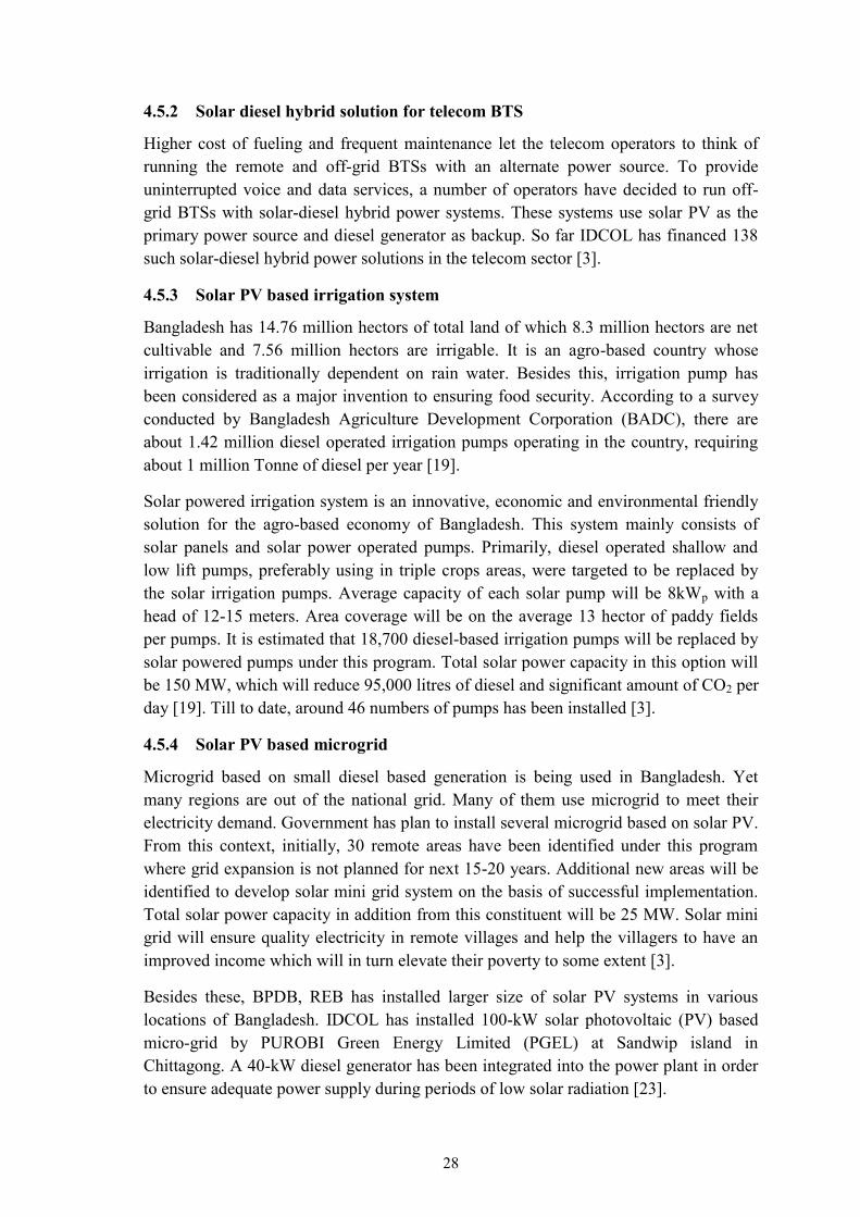
Figure 4.19 The total and average consumption of those users for the last three years (2011~2013).

44

Figure 4.20 The total and average consumption of those users for the last three years (2011~2013).

44

Figure 4.21 The average consumption of those users for the last three years (2011~2013).

45

Figure 4.22 The scaled up representation of Figure 4.21. 45

Figure 4.23 The number of maximum occurrence of minimum shortage for r=0.01% (tilt angle vs Frequency of occurrences).

46

Figure 4.24 The number of maximum occurrence of minimum shortage for r=0.1% (tilt angle vs Frequency of occurrences).

46

Figure 4.25 The number of maximum occurrence of minimum shortage for r=1% (tilt angle vs Frequency of occurrences).

47


47

xiv


Page No


48


48

Figure 4.29 The demand, generation and surplus/shortage for 230 and 90 tilt angle. 49

Figure 5.1 Monthly predicted average demand for 100 number of typical village family.

50

Figure 5.2 Demand, generation, shortage/surplus for various sizes of PV panels.

51

Figure 5.3 The optimum scale of the solar PV for minimum shortage and minimum surplus.

54

Figure 6.1 Recalling Figure 3.7 and Figure 3.9. 58

Figure 6.2 Ring diagram of a new microgrid model, where the generation and consumption will take place at the same point.

59

Figure 6.3 Several layers of the proposed microgrid, where closeness of the rings shows the integrity of generation and consumption.

59

Figure 6.4 Two different rings expressing the consumer and producer units have been merged into a single ring keeping the distribution close to the generation and consumption.

60

Figure 6.5 Discretely developed microgrids, may be interconnected. 60

Figure 6.5 Block diagram of Consumer Producer Unit (CPU). 61

Figure 6.7 CPU based Microgrid. 62

Figure 6.8 Interconnection of Microgrid with central controller. 62

Figure 6.9 Microgrid Network. 63

Figure 6.10 Microgrid connected to national grid. 63

Figure 6.11 Two CPU based isolated microgrid are expressed by equivalent thevenin circuit.

64

Figure 6.12 Resistance, Inductance and capacitance of the line and equivalent. 64

Figure 6.13 Capacitance of the line and its equivalent. 64

Figure 6.14 Equivalent circuit of the inter-connection line. 65

xv


Page No

Figure 6.15 Voltage drop vs Distance of interconnection. 66

Figure 7.1 Demand and generation for the default tilt angle (230) and optimum tilt angle (120) -case study Dhaka.

73

Figure 7.2 Demand met for default and optimum tilt angle-case study Dhaka. 73

Figure 7.3 Shortage at default tilt and optimum tilt angle position- case study Dhaka.

74

Figure 7.4 Demand and generation for the default tilt angle (230) and optimum tilt angle (90)-Case study Sandwip.

75

Figure 7.5 Demand met for optimum and default tilt angle-Case study Sandwip.

75

Figure 7.6 Shortage at default tilt and optimum tilt angle-case study Sandwip. 75

Figure 7.7 Price of purchase of energy from entity 2 VS period of return of initial investment for both of entity 1 and entity 2 while the selling price of energy by entity 1 is 20 Tk.

81


81


81


82

Figure 7.11 Payback period of the initial investment for both of entity 1 and entity 2 while the selling price of entity 2 is 10Tk.

82


83


83


83

Figure 7.15 Forecasted installed capacity of the proposed model based on IDCOL‟s installation number.

86

xvi

LIST OF TABLES

Table No. Title of the Table Page No

Table 2.1 Installed capacities of power plants in Bangladesh according to fuel.

7

Table 2.2 Various authorities, de-rated capacity and their market share. 8

Table 2.3 Cost of generation and purchase for various types of fuel. 8

Table 2.4 Percentage of the generation and its corresponding fuel costs. 9

Table 2.5 Year wise peak demand forecast. 9

Table 2.6 The share of electricity distribution by the relevant authorities 10

Table 4.1 The outputs of a 1kWp solar PV panel at different location of Bangldesh at its default tilt angle (latitude).

34

Table 4.2 The availabe irradiance at different location of Bangldesh 35

Table 4.3 The outputs of a 100kWp solar PV panel at different tilt angle, location is chosen as Dhaka

36

Table 6.1 Initial investment for entity 1 68

Table 6.2 Per year calculation for entity 1 69

Table 6.3 Initial investment for Entity 2 70

Table 6.4 Yearly cost calculation for entity 2 70

Table 7.1 The correlation co-efficient (CC) of generation at Dhaka with national demand profile and generation at Chittagong with Sandwip microgrid demand profile.

72

Table 7.2 The optimization according to the cost of energy 77

Table 7.3 Comparison of SHS and “Consumer is Producer” model 85

Table 7.4 Table 7.4: Possible installation capacity of the proposed “Consumer is Producer” model

86

xvii

ABBREVIATIONS

AAAC All Aluminium Alloy Conductors

AC Air Conditioner Or Alternating Current

ACSR Aluminium-Conductor Steel-Reinforced

ADB Asian Development Bank

APSCL Ashuganj Power Station Company Ltd.

BADC Bangladesh Agriculture Development Corporation

BERC Bangladesh Energy Regulatory Commission

BDT Bangladeshi Taka

BPDB Bangladesh Power Development Board

BTS Base Transceiver Station

BWDB Water Development Board

CC Correlation Co-Efficient

CG Centralized Generation

CPU Consumer Producer Unit

DC Direct Current

DESCO Dhaka Electric Supply Company

DER Distributed Energy Resource

DFID Department For International Development (Dfid)

DPDC Dhaka Power Distribution Company

EGCB Electricity Generation Company Of Bangladesh

FO Furnace Oil

FY 2013 Fiscal Year

GPOBA Global Partnership Of Output-Based Aid

xviii

ABBREVIATIONS

GOB Government Of Bangladesh

GTS Gas Turbines

GWH Giga Watt Hour

HFO Heavy Fuel Oil

HSD High Speed Diesel

HVDC High Voltage Direct Current

IDCOL Infrastructure Development Company Ltd

IPP Independent Power Producers

KfW Kreditanstalt Für Wiederaufbau (German Development Bank)

KV Kilo Volt

KWH Kilo Watt Hour

MVA Mega Volt Ampere

MW Mega Watt

MPEMR Power Division, Ministry Of Power, Energy & Mineral Resources

NGOS Non-Governmental Organizations

NREL National Renewable Energy Lab

NWPGCL North West Power Generation Company Ltd.

PBS Palli Bidyut Samiti

PGCB Power Grid Company Bangladesh

PGEL Purobi Green Energy Limited

PO Partner Organizations

PSMP Power System Master Plan

PV Photovoltaic

xix

ABBREVIATIONS

REB Rural Electrification Board

SHS Solar Home System

SNV Stichting Nederlandse Vrijwilligers (Netherlands Development Organisation)

STS Steam Turbines

T&D Transmission And Distribution

USAID United States Agency For International Development

WZPDCL West Zone Power Distribution Company Limited

XLPE Cross-Linked Poly Ethylene

1

CHAPTER 1

INTRODUCTION

Bangladesh is a developing country with huge population. Development of a country mostly depends on ensuring reliable and quality power to everywhere in the country. Due to unavailability of transmission and distribution network infrastructure, about 45% [1] of the population of Bangladesh remains off grid. Moreover, the grid areas are facing acute load shedding for lack of adequate generation. Per capita electricity generation of Bangladesh is 321KWh [2]. Bangladesh Government has set up its goal to ensure reliable and quality supply of electricity at a reasonable and affordable price to all by 2021 [1]. For sustainable social and economic development, it needs adequate power generation capacity.

People in the off grid areas of Bangladesh are mainly using fuel-based lamps as the lighting sources. Some of them are using electricity by means of local grid based on diesel/petrol generators that run for a few hours in a day. Some people use storage battery to be charged from the local grid or from the nearest national grid and use it for powering direct current (DC) light bulbs, small fans and black and white televisions for weeks. Besides these, the Solar Home System (SHS) of Infrastructure Development Company Ltd (IDCOL) offers the best way to the battery charging based electricity practice [3].

People had a nice feeling when they experienced the benefit of using a switch-based higher luminous bulb through SHS instead of oil-based lower luminous lamp. However, with the advancement of modern technology and globalization, the energy demand of existing users of SHSs is also increasing day by day. They are now willing to use ceiling fans, Television (TV), computer, blender, fridge, domestic water pump, air conditioner (AC) and other domestic appliances as well.

The Renewable Energy Policy of the government of Bangladesh envisions that 5% of the total energy production will have to be achieved by 2015 and 10% by 2020 [4], [5]. Power generation by fuel diversification is the best way to accelerate the development of renewable energy. There is no doubt that a higher penetration of renewable energy in the overall energy consumption will reduce the greenhouse effect drastically. 1.1 Literature Review

The electricity generation of the country is dependent mostly on the natural gas; a small part of the generation comes from hydro, oil and coal. Under the existing generation scenario of Bangladesh, a major portion of the generated electricity comes from natural gas, which is about 80% [1] of the total generation and is not enough to serve the demand. Other sources of energy are oil and coal. Due to shortfall of natural gas,

2

generation units often fail to reach its rated capacity. On the other hand, oil is being subsidized. Moreover, the prime concern about this type of fuel is the emission of carbon-di-oxide (CO2) which accelerates the greenhouse effect and thus the global warming. The only renewable energy source of the country that is connected to the grid, is the Kaptai Hydro power plant, which has a very small share (around 2. 58%) [1] of the total generation. Apart from this, some small and remote areas are being served by diesel generators by means of a local grid, which is defined as a microgrid [6]-[8]. Demand can also be met by connecting several microgrids locally, where installation of additional transmission lines, as in the conventional power stations, is not necessary as the sources are closer to the consumer and discretely located at different places of the microgrid. The discretely situated distributed energy resources (DERs) are being used as a supplement and an alternative to large conventional central power systems worldwide [9]-[11] and the penetration of DERs at medium and low voltage levels is increasing [12]-[14]. In those countries, the size of the DERs is large and most of them are interconnected to the national grid. The size of the energy resources used in local microgrid in Bangladesh is small and the scale of the microgrids is also small because of less electricity demand. The energy resources used in the isolated microgrids that are setup by the local people to meet their own needs are centralized. The available renewable energy sources in Bangladesh may be used as DER in a microgrid, which may meet a significant proportion of the national demand of electricity with a competitive price compared to the traditional power plants. Analysis of various factors by using large-sized DERs has been carried out in those countries. However, for the proposed small scale microgrid in Bangladesh, the size of the DERs will be small and decentralized. The analysis of the relevant factors of such scheme has not yet been carried out. We proposed to make the use of the available small scale energy resources in a decentralized manner in our small scale microgrid. 1.2 Scope of the Current Work

The available renewable energy resources in Bangladesh are hydro, solar, wind, biomass, tidal and wave, and geothermal. Among them hydroelectric power shares the maximum generation capacity of 230MW. Potential of Solar photovoltaic (PV) is available all over the country. Solar PV programs have also gained a large number of installations [3]. There are some suitable locations for installing wind farms of which few are in operation, some are in maintenance and many of them are in feasibility study. The biogas sector is also enriching, but most of the biogas plants are not used to generate electricity, rather they are used for cooking. The potentials of tidal, wave and micro hydro are promising but those are also at the level of feasibility study. The potential of extracting geothermal energy is little for Bangladesh. Using the solar PV resources and other available resources, it is possible to generate electricity that would be adequate to meet the local demand. This principle could be used all over the country. This is how a significant percentage of population may be brought under the electricity coverage region.

3

1.3 Objectives

The objectives of this research are: (a) To study the available resources of the renewable energy at various places of

Bangladesh. (b) To study the evacuation system of the national grid and the present microgrid

located at different places in the country. (c) To study the national load profile and microgrid load profile. (d) To search for an alternative and supplement to further extension of the present

power system. (e) To design a mathematical model for the proposed alternative. (f) To compare the performance of the proposed alternative with that of the

traditional system. 1.4 Features of the Alternative to the Present Power System

The alternative to the present power system is expected to have the following features: (a) Be suitable for the remote area considering the area, density of population,

load profile, availabilities of alternative power resources. (b) Be economically feasible and cost effective. (c) Create market for the common people. As a result, acceleration into the power

business should be possible. (d) Minimize the cost and loss associated with the evacuation. (e) Eliminate the transmission network as well as primary distribution network, by

low-level secondary distribution networks. (f) Decrease the Carbon emission as well as lower greenhouse gas emission and

decelerate the higher rate of global warming. (g) Have a reliable load management system as well as source management

system. (h) Be reliable for the extreme critical condition of the power system. (i) Be easy to install and easy to maintain. The plug and play type easier

installation could ensure the minimum installation time. (j) Minimum installation and running cost.

4

1.6 Methodology

The methodology of the research work may be shown by the following flow chart.

1.7 Layout of the Dissertation

Chapter 1 introduces the present scenario of electricity demand and generation of Bangladesh and emphasizes the necessity of an alternative and supplement to the existing power system.

Chapter 2 describes the available topologies for electricity generation and its evacuation system in Bangladesh.

Chapter 3 discusses the centralized generation system and the distributed generation system as well as the national grid and the local microgrids.

Chapter 4 describes the available renewable energy resources and its potential for Bangladesh.

Chapter 5 introduces a novel model that has been proposed for an electrical microgrid in a remote area based on the available distributed energy resources.

Chapter 6 explores a new model to generate electricity with higher penetration rate of renewable energy.

Chapter 7 shows some of the results obtained from the proposed model with the help of the developed software routines.

Chapter 8 summarizes the findings and achievements of the current research. It also suggests some possible extensions to substantiate the current research in future.

Comparing the performance of the proposed model with that of the conventional ones

Designing an appropriate mathematical model

Looking for the suitable criteria for a new model

Analysis of the National grid and Microgrids

Resource Analysis

5

CHAPTER 2

A REVIEW ON ELECTRICITY GENERATION AND

EVACUATION SYSTEM IN BANGLADESH

This chapter describes the available topologies for electricity generation and its

evacuation system in Bangladesh. Usually, electricity is generated in a large power

station and it is then sent to the customer end by means of transmission and

distribution systems. This is an established technology. However, this system proves

very costly and the cost increases especially when the service area is remote. In

remote areas, local people use kerosene as a fuel for lighting. Also, diesel generators

for electrifying local markets and villages are being used. However, these generators

run for a few hours of the day and the generation cost becomes very high. Practice of

battery charging based electricity system is also found in many places of the remote

area. Besides these, Government of Bangladesh (GOB) is trying to electrify the remote

areas by means of SHS, which has been being used to replace the traditional kerosene-

based lamps from 1998 in Bangladesh. However, with the advancement of technology,

the new demand for SHSs and more energy demand of existing SHS consumers is also

increasing considerably. Electricity to all is an essential requirement for the proper

development of Bangladesh. Thus, it is essential to supply power with quality and

reliability to the present users of the national grid, customers of the SHS and people of

the un-electrified region. With this context, possibilities of exploring new topologies of

generation and evacuation have also been discussed in this chapter.

2.1 Electricity Generation and the Grid

Producing electrical power by means of any energy conversion method is known as electricity generation. Large scale electricity is basically produced from rotary machines such as gas turbine, steam turbine, hydro-turbine and engines etc. The necessary systems that are needed to transfer power from the generating unit to the customer end are known as the evacuation system.

Bangladesh is a small country with large amount of population. Presently, 55% [1] of the total population has access to electricity and per capita generation is 321KWh [2]., which is very low compared to other developing countries. There are mainly three major methods or topologies of supplying electricity to the customers in Bangladesh.

The first one is the traditional large-scale centralized generation, where electricity is generated from hydroelectric power plants, gas turbines, steam turbines, gas engines and diesel engines and by many other means. In a hydroelectric power plant, potential energy of the reserved water is converted into electrical energy. The cost involvement is

6

only for installation, operation and maintenance. On the other hand, steam Turbines (STs), Gas Turbines (GTs) or engine generators are based on fuel such as natural gas, High Speed Diesel (HSD), Furnace Oil (FO), Coal etc. The concerned authority of the Government of Bangladesh, Bangladesh Power Development Board (BPDB) is generating power by its own generators as well as purchasing electricity from other private companies [1]. Whoever produces the electricity is then transmitted and distributed to the consumer end by means of the available transmission and distribution (T&D) system. The T&D system needs special infrastructure, which is very costly [2].

The second one may be termed as the single unit generation i.e. a standalone system that does not need any T&D system such as the solar home system (SHS), solar irrigation system etc. Along with the centralized generation, till now (October, 2014) more than 3 million (3,258,653) SHSs have already been installed in the off-grid rural areas of Bangladesh under the program run by IDCOL with the co-operation of several Non-Governmental Organizations (NGOs). As a result, more than 13 million beneficiaries are getting solar electricity, which is around 9% of the total population of Bangladesh. Most of the installed SHS units are used at home, few of them are used in educational institutions, prayer houses and shops in the market. A SHS is able to provide electricity for a few light bulbs, small DC fan and TV, rechargeable torchlights and adapters for mobile phone charging [3].

The third method of supplying electricity is the local grids run by small-scale diesel/petrol engines at the remote areas. These topologies are shown in the following flow chart in Figure 2.1. Local grid is shown between the extreme two cases.

Figure 2.1: Three topologies of generation and evacuation of electricity in Bangladesh.

Unfortunately, the third method of supplying electricity has not been taken into consideration by the policy makers and has so far remained neglected. These generation units are distributed all over the remote areas of the country and are not interconnected

7

in any way. The generated energy is locally consumed with a low voltage distribution line. However, generation cost is also high in this case. These are operated by local electricians/operators in most of the cases and thus it has enough risks of electrical hazards.

2.2 Generation

Most of the power stations in Bangladesh are based on natural gas, which is around 80% of the total capacity on the fiscal year (FY) 2013 [1]. On the other hand, gas is short supply and about 1500 MW of generation shortfall occurs in a day due to shortage of gas [15]. Therefore, it will be very tough to provide more electricity generated from the natural gas in future. The daily reports of Power Grid Company Bangladesh (PGCB) show the decreasing supply of natural gas and more and more penetration of oil-based generation. Government of Bangladesh is trying some alternative to natural gas such as coal, HSD and Furnace oil based power plants under the fuel diversification program [1]. So far, as the fuel is concerned, the generation capacity is 6,719 MW by Natural Gas, 1,963 MW by heavy fuel oil (HFO), 783 MW by high speed diesel (HSD), 230 MW by Hydro and 200 MW by Coal. Besides these, 500MW has been imported from India since November, 2013 via high voltage direct current (HVDC) transmission line. Table 2.1 shows the installed capacity of Power Plants in Bangladesh according to fuel [16].

Table 2.1 Installed capacities of power plants in Bangladesh according to fuel.

Unit Type Capacity(Unit) Total (%) Coal 250.00 MW 2.39 % Gas 6719.00 MW 64.33 %

HFO 1963.00 MW 18.79 % HSD 783.00 MW 7.5 %

Hydro 230.00 MW 2.2 % Imported 500.00 MW 4.79 %

Total 10445.00 MW 100 %

Presently, the use of natural gas, HSD, Coal and HFO are around 80%, 10%, 5%, and 3% [15], respectively of the total generation. Bulk of the power in Bangladesh is generated by BPDB. There are other independent power sources as well.

Power Division, Ministry of Power, Energy & Mineral Resources (MPEMR), and Bangladesh Energy Regulatory Commission (BERC) are the governing bodies of Power Sector of Bangladesh.

The following authorities are responsible for generating electricity in Bangladesh.

(i) Bangladesh Power Development Board (BPDB) (ii) Ashuganj Power Station Company Ltd. (APSCL) (iii) Electricity Generation Company of Bangladesh (EGCB) (iv) North West Power Generation Company Ltd. (NWPGCL) (v) Independent Power Producers (IPPs)

8

Table 2.2 shows the de-rated generation capacity and their market share for the five authorities of electricity generation [16].

Table 2.2: Various authorities, de-rated capacity and their market share.

SL No Name of the Authorities Capacity Market Share

01 Bangladesh Power Development Board (BPDB) 4442 42.75%

02 Ashuganj Power Station Company Ltd. (APSCL) 682. 6.56% 03 Electricity Generation Company of Bangladesh (EGCB) 622 5.98% 04 North West Power Generation Company Ltd. (NWPGCL) 375 3.06% 05 Independent Power Producers (IPPs) 4269 41.08% Total 10390 100%

All the generated power are purchased by the BPDB and then transmitted by PGCB to the customers‟ premises. The generation cost and purchase cost of each unit (KWh) of electricity is shown in the table 2.3 below [1]. The Snapshots of these costs are given at Appendix-A.

Table 2.3: Cost of generation and purchase for various types of fuel.

Purchase cost Type Maximum Cost / Tk. per unit Average Cost / Tk. per unit Rental Gas 5.97 4.58 Rental HFO 25.70 17.58 Rental Diesel 35.03 27.24 Rental Average 10.99 Generation Cost Hydro 0.88 0.88 Gas 5.87 1.97 Coal 5.71 5.71 HFO 50.60 17.85 Diesel 53.63 43.91 Total Average of Generation and Purchase 3.80

Till September, 2014 the total generation capacity of Bangladesh is 10,445 MW the de-rated capacity is 10,390 [16]. It should be noted here that 3.11% and 11.95% of generated energy are lost due to transmission and distribution, respectively [1].

The major part of the generation comes from the natural gas, for which the cost of generation of per unit energy is lower. However, it is higher for HSD and HFO due to high price. Energy Flow Chart of FY 2013 [1] shows that 77.91GWh of energy is produced from 34.79 Million liters of Diesel costing diesel of about 30.364 Bangladeshi taka (BDT) per kWh of energy whereas it is 13.46BDT for Furnace oil, 3.7BDT for coal

9

and 0.902BDT for gas-based generation on an average (only for BPDB Generation). However, these costs are only for fuel. The actual cost is much higher when other running and maintenance costs are included. It should be noted here that the overall thermal efficiency of the power plants is 33% and the annual plant factor is 45.02%. Table 2.4 shows the percentage of the generation and its corresponding costs for various types of fuel for BPDB only [1]. These data are only for the generation of BPDB and other generations are not included here. This could be found at Appendix-A.

Table 2.4: Percentage of the generation and its corresponding fuel costs.

Fuel Type % of Total Generation % of Total Fuel Cost

Diesel Oil 1.805979438% 28.3247319% Furnace Oil 2.136239115% 24.4400091% Coal 5.894480959% 10.9173104% Natural Gas 85.08369443% 36.3179485% Water 5.079606058% -

Based upon the preliminary study of the Power System Master Plan (PSMP) -2010, the anticipated peak demand would be about 10,283 MW in FY2015, 17,304 MW in FY2020 and 25,199 MW in 2025. The policy envisions 800MW of power from renewable energy by 2015 and 200MW of power by 2020[17]. According to PSMP- 2010 Study year-wise peak demand forecast is shown in Table 2.5.

Table 2.5: Year wise peak demand forecast.

Fiscal Year 20

10

2011

20

12

2013

20

14

2015

20

16

2017

20

18

2019

20

20

2021

20

22

2023

20

24

2025

20

26

2027

20

28

2029

20

30

Peak Demand (MW) 6,

454

6,76

5 7,

518

8,34

9 9,

268

10,2

83

11,4

05

12,6

44

14,0

14

15,5

27

17,3

04

18,8

38

20,4

43

21,9

93

23,5

81

25,1

99

26,8

38

28,4

87

30,1

34

31,8

73

33,7

08

2.3 Transmission and Distribution

The only company that works for the transmission of electricity in Bangladesh is the Power Grid Company of Bangladesh Ltd. (PGCB).

As of June 2013, there is almost 3,020 km of 230 kV and 6,148 km of 132 kV transmission line available in the country. The number of 230/132 kV substations is 16 and combined capacity of those entire substations is 7,525 MVA. Besides, there are 103 substations of 132/33 kV available throughout the country with a capacity of 11,792 MVA. The distribution network is the biggest of the lot, with 3,728 km, 13,128 km and 21,839 km of 33 kV, 11 kV and 400 V lines, respectively. There are 158 substations of 33/11 kV for distribution of power around the country [2].

10

Four companies are distributing the generated power along with BPDB. BPDB is responsible for distribution of electricity in most of the urban areas in Bangladesh except Dhaka Metropolitan City and its adjoining areas under Dhaka Power Distribution Company Limited (DPDC) and Dhaka Electric Supply Company Ltd. (DESCO), areas under West Zone Power Distribution Company Limited (WZPDCL) and some of the rural areas under Rural Electrification Board (REB). The Distribution Zones of BPDB are Chittagong, Comilla, Sylhet, Mymenshing, Rajshahi, Rangpur. 40.10% of the said generated power is purchased by REB and distributed to the pastoral area. BPDB distributes 24.64% of the power among the urban consumers. DPDC and DESCO distribute 18.59% and 10.51% respectively, of the power among the consumers in Dhaka metropolitan area. The rest 6.17% of the power is distributed by WZPDC in Khulna and Barisal divisions [1]. 46.52% of the power is used for resident loads, 10.34% for commercial purposes, 37.42% for industries, 3.17% for agriculture and 2.56% for other purposes [1]. The share of electricity distribution by the relevant authorities has been shown in Table 2.6.

Table 2.6: The share of electricity distribution by the relevant authorities

Authority BPDB DPDC DESCO REB WZPDC

Share in Percentage 24.64% 18.59% 10.51% 40.10% 6.17%

Among the distribution authority, REB has the highest share of electricity distribution. REB is working through Palli Bidyut Samiti (PBS) working over the country. The customer density of PBS is around 35. The urban areas are denser than rural areas. The customer densities of several PBSs are shown in Figure 2.2.

Figure 2.2: Customer density of PBS for several districts.

11

The summary of the length of transmission and distribution lines at various levels is given below:

(a) 230KV:1324.40 km route and 3020 ckt km Used conductor: Mallard, twin mallard, Twin AAAC, finch, ACSR

(b) 132KV: 3505km, 6148 ckt km Used conductor: Grosbeak, AAAC, HAWK, Cu.Cable, XLPE, Twin AAAC

(c) 33KV feeder length:3728km (d) 11KV feeder length: 13128km (e) 0.4KV feeder length: 21839km

2.4 Local Mini Grids

There are a number of local grids in the remote areas of Bangladesh. Most of the local grids in Bangladesh are run by diesel generators. Remote villages and markets have local grids. However, the electricity is available only for a few hours, and used mainly for lighting purposes only. Most of the grids have a generation scale of 5kW ~ 10kW diesel generators serving about 20~50 number of customers/shops.

These grids may be defined as mini grid or micro grid. In a microgrid, no transmission line is needed, only low voltage distribution lines are necessary. Here, bamboo poles or other supporting elements are used instead of the standard poles. The generation cost is around 30Tk per kWh. However, a customer is charged around 50Tk. per kWh.

Besides these, solar PV based mini-grid projects are installed in remote areas of the country, where possibility of grid expansion is remote in the near future. These projects provide grid quality electricity to households and small commercial users, and thereby encourage commercial activities in the project areas.

So far, IDCOL has financed one 100 kWp solar microgrid project in Sandwip Island. The project is currently supplying electricity to adjacent 250 shops, 5 health centers and 5 schools. Another four projects of different capacity (100~159 kWp) have been approved by IDCOL which are in various stages of construction. IDCOL has a target to finance 50 such solar mini-grid projects by 2017. 2.5 Complete Stand-Alone System

A complete stand-alone system has no distribution system. The generated electricity is sent to the load directly or via a storage device. Such an application is solar home system (SHS).

At present 47 Partner Organizations (PO) are implementing the program under the supervision of IDCOL. More than 3 million SHSs have already been installed under the program in the off-grid rural areas of Bangladesh. As a result, 13 million beneficiaries are getting solar electricity, which is around 10% of the total population of Bangladesh. More than 65,000 SHSs are now being installed every month under the program. IDCOL has a target to finance 6 million SHSs by 2017, with an estimated generation capacity of 220 MW of electricity.

12

Solar Photo Voltaic (PV) is used to convert the energy of sunlight into electrical energy. The unit is named as solar cell, it is a junction made from the p-type and n-type semiconductor (silicon). Incident light ray with certain wavelength will make emission of electron from the junction producing flow of electron or electric current. Several cells will form a solar panel/module and several panels/modules will form a solar array.

The electricity generated from the sunlight by the solar PV panel could be utilized in several ways. Due to some limitation, this energy cannot always be used directly to the load. At night the production is zero and at foggy, cloudy or rainy day the output is very low. This is called intermittent source [18]. Due to the intermittency, output of the panel is not constant; it just fluctuates. This fluctuation may hamper the load and may even damage it. Hence, most of the application needs battery as a backup to solve the problem of intermittency except the solar irrigation system, solar PV based battery charging station, grid tie system etc. For a larger system other resources may be used. SHS is remarkable among the application of solar PV. Conventional SHS have light bulbs as load that runs at night. In some cases, low power DC fan and TV are also used. The only way to use this electricity at night is to store the energy in a battery. Therefore, in this system battery is mandatory. Storing the electricity produced by the panel into the battery is known as charging and using the storage energy from the battery by the load is known as discharging. The length of duration while the battery can store and deliver the energy to the load properly is defined as the life time of the battery. It is specified by the number of cycle it is charged and discharged as well as years of operation. If the charging and the discharging are not taken place properly, the life time of the battery will be decreased. Too much charging or discharging is bad for the battery. To ensure this operation properly a charge controller is used. It may be compared to the brain of the total system. It will protect the battery, panel and the load from current reversal, overcharging, deep discharging, short-circuit and other bad impacts. The complete process is shown in the block diagram of Figure 2.3.

Figure 2.3: Block diagram of a SHS showing the Panel, Battery, Charge Controller and Load.

13

2.6 Possibilities of Using Electrical Microgrids in Bangladesh

As discussed earlier, a conventional power system consists of large-scale power stations, transmission lines, substations and distribution lines etc., where the generation and consumption of power are not at the same location. Due to unavailability of enough T&D lines, remote areas are normally not connected with the electrical grid, thus these areas are deprived of development. On the other hand, SHS is being used drastically at the remote areas. Although the number of installed SHS unit is high enough, the total amount of electricity produced by these is not significant yet. Moreover, this is not a permanent solution of electricity. In this context, a local grid may offer a better alternative. Government has planned to install several microgrids at some selected region to add more power in the national generation from the renewable energy sector. Also, the Government has a plan to replace 19,000 number of diesel pumps with the solar PV system as well as installing some mini-grids at various remote sites [19].

Owing to some important factors as will be discussed next, it is a high time to think of the higher penetration of renewable energy into the generation of electricity in a decentralized manner as proposed. For the traditional power generation systems, fuel cost for oil-based plants is high and sometimes it exceeds 30Tk per KWh [1]. The generation cost of natural gas based electricity is lower but, the reserve of our natural gas is going to be diminished very soon. Shortfall of generation due to shortage of enough supply of natural gas is common for generation [15]. Besides these, most of the generation units emit high amount of CO2 which increases the greenhouse effect and the global warming. In addition, the cost and loss associated with the evacuation system is not negligible either. Moreover, interruption at any node in the grid turns into load shading and hampers a lot of users, when many customers get completely disconnected from the grid.

If the generation units (diesel generator) of local grids could be replaced by the solar PV as well as creating new small grid based on solar PV, and these grids could be interconnected to some extent, the problem of electrifying the remote areas may be solved in a greater degree[27]. For example, a 10MW capacity power station may be replaced by installing 1000 number of generating units with 10KW capacity each, which are situated at different locations through an interconnected gird. It would not require any transmission network; rather a low voltage distribution network may be used for the distributed generation.

Similarly, if the outputs of each PV panels are interconnected locally, then it would be able to provide the required energy sufficient for all the users of the locality by means of a Microgrid [7]-[8]. A microgrid is a group of interconnected loads and distributed energy resources (DERs) within clearly defined electrical boundaries that acts as a single controllable entity with respect to the grid. A microgrid can be connected and disconnected from the grid to enable it to operate both in grid-connected or in island-mode [20]. The available renewable energy sources in Bangladesh may be used as DERs in a microgrid, which will reduce the control burden on the grid and may meet a

14

significant proportion of the national demand of electricity with a competitive price compared to the traditional power plants. The penetration of DER based microgrid is increasing in the developing country day by day. Moreover, a microgrid can be interconnected to any adjacent microgrid in case of emergency. Interconnected microgrids have more opportunities to share generated power among various loads and make it easier for load management and control. With proper design and implementation, interconnected microgrids have ample scope to be connected with the national grid without the need of installing new transmission lines [14]. I. 2.7 Summary

Considering the possibilities of incorporating electrical microgrids, new models for generation and distribution of electricity should be in the agenda of power planning cell of the Government of Bangladesh. It is expected that by incorporating electrical microgrid, transmission and distribution loss and overall cost of electricity production will be minimized significantly. Also, the emission of CO2 will be negligible with a new load management technique, and reliable and high quality power may be ensured within the shortest possible time. The proposed model could be used as an alternative to the bulk scale generation and supplement the traditional power system. Installation of large power plant based on renewable energy resources is good. However, the scope of implementation is not available everywhere in Bangladesh. Moreover, it also needs the evacuation system, which is still costly even though loss has been minimized. On the other hand, the installed number of SHSs in the country is huge (more than 3 million) but its share to the total generation is not that significant. Moreover, it is not contributing to the national grid in any way. Therefore, proper sizing of the power sources are important as well as designing the appropriate evacuation system. Keeping this context in mind, distributed energy resources and the microgrid are discussed in the next chapter.

15

CHAPTER 3

DISTRIBUTED ENERGY RESOURCES AND THE MICROGRID

The last chapter reviewed the electricity generation and evacuation system in Bangladesh. This chapter discusses the centralized generation system, distributed generation system, the national grid and the microgrid. A credible alternative generation paradigm, distributed generation has been discussed to overcome significant technical, economic, regulatory and environmental hurdles. Electricity is mainly produced at large generation facilities, shipped through the transmission and distribution grids to the end consumers. However, the recent quest for energy efficiency and reliability and reduction of greenhouse gas emissions led to explore the possibilities to alter the current generation paradigm and increase its overall performance. In this context, one of the best alternatives, complements or even replacing paradigm is the distributed generation, where electricity is produced next to its point of use. Distributed Energy Resources (DERs) can provide solutions to overcome the shortfalls of the centralized generation. Environmental concerns also led regulators to promote efficient generation technologies. 3.1 Distributed Energy Resources

In Bangladesh, most of the power is generated from large-scale traditional centralized power stations. The generated power reach to the consumer through transmission and distribution (T&D) network associating higher loss and cost. The remote areas increase the cost and loss much more. However, large-scale power can be generated by multiple smaller scale power generation units, which are located at several locations within the entire service area. This is also known as decentralized generation or distributed generation, generating power in a decentralized manner [7].

For example, 500MW of power may be generated in a single power station or it may be generated by installing 500 numbers of generating units of 1MW, which are situated at different locations throughout the gird. Decentralization of generation removes the transmission network and only a low voltage distribution network is associated with it.

Distributed energy resources are small, modular, energy generation and storage technologies that provide electric capacity or energy where it is needed. There are options to be either connected to the local electric power grid or isolated from the grid in stand-alone applications for DER based system. DER technologies include wind turbines, photovoltaic (PV), fuel cells, micro-turbines, reciprocating engines, combustion turbines, cogeneration, and energy storage systems [21].

Distributed energy generation is a local and decentralized energy production system. A decentralized energy system is characterized by locating of energy production facilities

16

closer to the site of energy consumption. As a relatively new field of research, several expressions are still currently used such as “decentralized generation”, “dispersed generation”, or “distributed energy resources” etc [22].

Distributed generation may be defines as a generator with small capacity close to its load that is not part of a centralized generation system. Also it is such kind electric power source that is connected directly to the distribution network or on the customer site of the meter. The key criteria in the definition of DER are the connection to the distribution network and the proximity to the end consumer.

The complete discussion on the distributed generation system may be exemplified with the following example and Figure 3.1 to Figure 3.6.

Figure 3.1 shows that a large, remote, centralized and conventional power plant, which may be run by natural gas, oil, coal, nuclear or massive wind or hydro power plants connected to the power system. It needs transmission and distribution lines for energy consumption at the consumer end which is shown in Figure 3.4 and Figure 3.5.

Figure 3.1: Traditional power system.

On the other hand, the same amount of power may be generated from multiple numbers of smaller generating units, which is shown in Figure 3.2; this is an idea of distributed energy resources. However, the size and scale is an important factor. The size is yet too large (10MW) and is associated with transmission system.

17

Figure 3.2: Distributed Energy Resources (larger size needs both T&D).

Same idea could be applicable for a smaller distributed generation. Figure 3.3 shows smaller size of distributed energy resources, which needs no transmission system at all.

Figure 3.3: A DER (smaller size) based power system need no transmission line.

18

Figure 3.4 expresses same idea with a flow chart of power flow.

Figure 3.4: Flow chart of power flow in central generation and distributed generation. Figure 3.5 shows the idea of the traditional centralized power generation by a ring diagram, in a different way. Here, generation, transmission, distribution and consumer network all are shown by rings with different color and radius. The flow of power is also shown by the arrow.

Figure 3.5: The traditional power system with a central generation. The red ring/circle at the center denotes the central generation. The outer ring over the generation ring signifies the transmission layer. This ring has a color of purple. The ring after transmission layer which is blue in color is indicating the distribution layer. Thus, the outermost ring is indicating the consumption layer. The generations are not concentrated in a place rather and the units are distributed over the entire grid. However, this type of grid may have both primary (high voltage) and secondary (low voltage) distribution networks Figure 3.6 shows the distributed power system, where the legends are same as that in Figure 3.5.

19

Figure 3.6: Distributed power system with distribution network only.

3.2 Microgrid

An electrical microgrid is local grid, which mainly operates within a small area, having no transmission network, only low level of voltage distribution network is available in a microgrid [7]. It can operate in an island mode or have a scope to be connected with national grid. The links between the idea of the national gird and the microgrid can be easily explained in similar way of links of a big market in an urban area with the small village market. The products may be either centrally generated or distributed or the products may be produced and consumed within a locality. The traditional microgrid may be expressed by the following circle diagram (Figure 3.7) where, the generation unit small and centralized.

Figure 3.7: Traditional microgrid: having no transmission, only user voltage level of distribution. (Generation of power is centralized).

20

A microgrid is operating at Sandwip has the resources in a single unit. Figure 3.8 shows the solar PV- diesel microgrid structure at Sandwip Island. Details of this microgrid are included in Appendix –B.

Figure 3.8: Solar microgrid layout using four cluster “Sunny Island” inverter. However, the power sources of a microgrid may be decentralized as well. In fact, it has some advantages over a microgrid having central generation unit. There are multiple numbers of power units, which are distributed over the entire grid. Additions of new resources are easier to meet new increasing demand. This microgrid can be expressed by a similar circle diagram, of Figure 3.7. The several layers of a decentralized microgrid are shown in Figure 3.9.

Figure 3.9: DER based microgrid where generation is distributed over the entire area.

21

3.3 Levels of Microgrid Based on Power Consumption

The microgrids may be categorized by the following ways Based on Power Consumption:

(a) Urban Microgrid: Yet, many of the urban area is not electrified. Urban microgrids are available there.

(b) Rural Microgrid: Thousands of rural microgrids are operating to electrify the rural markets and villages.

(c) Industrial Microgrid: a grid of self-powered industry. (d) Remote Microgrid: 100kWp Sandwip Microgrid. (e) Interconnected Microgrid: No microgrid is interconnected in Bangladesh. (f) Islanded Microgrid: Most of the microgrids are islanded.

3.4 Why We Should Think of Distributed Generation

It is time to think of the distributed generation for several important reasons. These are summarized as follows:

(a) Higher installation cost, running and maintenance cost of centralized generation (CG).

(b) Loss and cost associated with transmission and distribution are high for CG. (c) Fluctuations of voltage and frequency for CG. (d) In CG, interruption at a node (generation, transmission or distribution)

hampers a lot of consumers, thus less reliable (e) Most of the generating stations in CG release carbon-di-oxide that is harmful

for the environmental. (f) Higher penetration of renewable energy is tough this.

3.5 Summary

Available microgrids in Bangladesh are mainly based on diesel generators. A few of them are based on biogas or other renewable energy sources. Whatever be the resources, the grids have small but central generation units. As the microgrids operate in a smaller region, people may in general think that the decentralized generations are less important. DER based larger grid are available in various parts of the world. However, a microgrid which has a scale suitable for Bangladesh must make use of the small-scale energy resources in a decentralized manner, which will prove to be more beneficial for Bangladesh. The next chapter will discuss the analysis and optimization of the available resources.

22

CHAPTER 4

ANALYSIS AND OPTIMIZATION OF THE AVAILABLE ENERGY RESOURCES

The last Chapter described the distributed energy resources and the microgrid. This Chapter describes the available renewable energy resources and its potential for Bangladesh. Among several renewable energy resources, the application of solar Photo Voltaic (PV) is more familiar though the largest plant based on renewable energy goes under hydroelectricity. Besides these, wind, biogas, mini hydro and tidal are also well known. GOB has a plan to generate 5% of the total energy from renewable energy resources within 2015 and 10% within 2020. Through the approved renewable energy policy, the GOB is committed to facilitate both public and private sector investments in renewable energy projects to substitute indigenous non-renewable energy resources and increase the contributions of renewable energy based electricity generation. With this context, analysis of the available renewable energy resources is essential. A new concept to maximize the energy usage from solar PV by changing the tilt angle and thus to minimize the shortage to meet a specific demand profile1 of an isolated power system is also introduced here. 4.1 Available Renewable Energy Resources

The possible electricity generations from the renewable energy sources in Bangladesh are as follows:

(a) Solar (b) Wind (c) Small hydro (d) Wave and tidal energy (e) Biogas and (f) Others

4.1.1 Solar

The sun is the source of all energy of the world. Wind, hydro, fuel, tidal and many other sources of energy directly or indirectly receive energy from sunlight. Sunlight is the light and energy that comes from the Sun. When this energy reaches the surface of the earth, it is called solar insolation. What we experience as sunlight is actually solar radiation. It is the radiation and heat from the Sun in the form of electromagnetic waves. Sunlight is a portion of the electromagnetic radiation given off by the Sun, in particular infrared, visible, and ultraviolet light. On Earth, sunlight is filtered through the atmosphere of the earth, and is obvious as daylight when the Sun is above the horizon.

1 Demand profile/pattern or load profile/pattern are used to express the same idea.

23

When the direct solar radiation is not blocked by clouds, it is experienced as sunshine, a combination of bright light and radiant heat. When it is blocked by the clouds or reflects off other objects, it is experienced as the diffused light.

Both light and heat of radiation can be used for our daily life. There are many ways to utilize the solar radiation such as direct heating of water, drying clothes, drying grains, generation of electricity etc. Generation of electricity may be accomplished by directly converting the light into electricity or using the heat energy as a source to boil the steam for a steam turbine. Solar power may be classified two categories, namely, solar thermal and solar photovoltaic (PV). However, only solar PV part will be discussed in this chapter for generating solar power.

The light energy of solar radiation can be converted into direct current of electricity by using a solar cell, which acts as the fundamental power conversion unit [28]. It is made from semi-conductor similar structure like diode. The solar cells are being made from different materials and different structure in the quest of maximum power with minimum cost. However, the efficiency of commercial cells is less than half of the value tested at laboratories. Among the several types of solar cell, poly-crystalline and mono-crystalline solar cells are mostly available. Besides these, amorphous and thin film solar cells are also available in the market [28].

Solar cells are arrangements of semiconductors to convert sunlight directly into electricity by exploiting photovoltaic effect. The incident energy of light creates mobile charged particles in the semiconductor, which are then separated by the device structure and used to produce electrical current.

4.1.2 Power loss in solar cells

The power losses in a solar cell may be discussed by fundamental loss, losses due to collection efficiency, series resistance losses and other losses. These are given below:

The fundamental losses Not the entire solar spectrum is utilized for converting into usable energy. The rest of the energy may be considered as primary loss. The conversion efficiency may be improved by using Tandem cell. Loss as heat dissipation is also significant for solar cell. Besides these, loss due to recombination is also a factor to decrease the overall efficiency. This is an opposite process of carrier generation. Both Voltage and current reduces due to recombination thus the generated power from the PV cell [28].

Impurities or defects in crystal structure or at the surface of the semi-conductor may introduce energy levels inside the energy gap. These energy levels act as stepping stones for the electrons to fall back into the valance band and recombine with the hole thus reducing the carrier. Loss due to the ohmic metal contacts to the semi-conductor is also a fundamental loss. With proper structural development, these losses could be reduced.

24

Loss due to collection efficiency Collection efficiency is defined as the ratio between the number of carriers generated and the number photon strikes the surface. Crystalline materials are good for achieving higher collection efficiencies. To increase the collection efficiency of amorphous or polycrystalline thin films are used. In this case, additional electric field are needed to pull the carriers [28].

Series resistance losses Transmission of electric current produced by the solar cell involves with ohmic losses. This loss may be expressed by an equivalent resistance. This loss mainly reduces the fill factor2[28].

Other losses (i) Loss due to light reflection from the top surface: this can be minimized by

anti-reflection coating and surface texturing (ii) Loss due to shading of cells by top contacts such as fingers and bars: Stanford

University has designed a new cell structure , where both of the contacts are moved to the back side.

(iii) Loss due to incomplete absorption of light: this loss could be minimized by using light trapping and making the back contact optically reflecting.

4.2 Effects of Temperature

Temperature has a negative co-efficient for voltage normally around -23mVK-1 for PV cells and positive co-efficient for current, which is very small and negligible [28]. These effects are shown in Figures 4.1.

Figure 4.1: The effect of temperature on current vs voltage curve.

The generated power of a solar cell decreases with increase of temperature. The maximum power points for various temperatures also move towards the origin when temperature is increased [28]. This effect is shown in Figure 4.2

2 Fill factor=Maximum Power produced by the cell/(Short circuit current*Open circuit voltage of the cell)

25

Figure 4.2: The effect of temperature on power vs voltage curve.

4.3 Effects of Irradiance

Short circuit current of a solar cell is directly proportional to the flux of photon with the band gap energy. The flux of photon increases with the irradiance. The irradiance has negligible effect on voltage. As a result, power is directly proportional to the irradiance of the radiation [28]. The effect of irradiance on current vs voltage curve is shown in Figure 4.3.

Figure 4.3: The effect of irradiance on current vs voltage curve.

26

The effect of irradiance on power vs voltage curve is shown in Figure 4.4.

Figure 4.4: The effect of irradiance on power vs voltage curve. The two curves are shown on the same plot in Figure 4.5

Figure 4.5: The effect of irradiance on power and current vs Voltage curve.

4.4 Effect of Angle of Incidence

Angle of incidence is an important factor. The number of incident photon is maximum when the incident ray is perpendicular to the plane of the solar panel. This can be described by the following equation.

I=Iocos(α) … … … … … …(4.1) where,

α is the tilt angle, the angle between the incident ray and the area vector of the panel plane, Io= received irradiance when α=0o and I= received irradiance when α=other than 0o

27

As the sun seems to move from east to west, the angle of incident also varies with position of the sun. On the other hand, the position of the locus of the sun is also changed with the year round. Therefore, this is another reason for the change of the incident angle of the ray.

To have maximum power output from a solar panel, a maximum power point tracker is being used worldwide. Single axis sun tracker has been developed for better daily performance and dual axis sun tracker has been developed for better yearly performance. However, the cost associated with the sun tracker and the additional spaces that are required for panels‟ movement (inter panel distance) have almost nullified the better performance of the sun tracker. 4.5 Application of Solar PV in Bangladesh

The application of solar PV is mainly found in remote areas of Bangladesh. IDCOL started the SHS program in 2003 to ensure access to clean electricity for the energy starved off-grid rural areas of Bangladesh. The program supplements the Government‟s vision of ensuring „Access to Electricity for All‟ by 2021. Besides these, hybrid microgird (with solar PV), solar PV based irrigation system, grid-tied solar PV system are also in action. These are described below. 4.5.1 Solar Home System

In Bangladesh, access to energy services for cooking and lighting in off-grid villages is slender. Most rural households have to rely on kerosene lamps for lighting and traditional stoves for cooking. The Government has initiated various programs and has given enormous efforts to introduce flexibility in rural economy.

Solar power, especially SHS technology, has been accepted by the rural people in reasonable way to meet their lighting needs. More than 3 million SHSs have already been installed under the program in the off-grid rural areas of Bangladesh [3]. As a result, 13 million beneficiaries are getting solar electricity, which is around 10% of the total population of Bangladesh. IDCOL has a target to finance 6 million SHSs by 2017, with an estimated generation capacity of 220 MW of electricity.

At present 47 Partner Organizations (POs) are implementing this program. IDCOL provides refinancing and grant support as well as necessary technical assistance to the POs. The POs install the SHSs, extend credit to the end users and provide after sales services. IDCOL received credit and grant support from the World Bank, JICA and others financial supporting organization [3].

More than 65,000 SHSs are now being installed every month under the program with average year to year installation growth of 58%. The program replaces 180,000 tons of kerosene having an estimated value of USD 225 million per year. Moreover, around 70,000 people are directly or indirectly involved with the program. The program has been acclaimed as one of the largest and the fastest growing off-grid renewable energy programs in the world [3].

28

4.5.2 Solar diesel hybrid solution for telecom BTS

Higher cost of fueling and frequent maintenance let the telecom operators to think of running the remote and off-grid BTSs with an alternate power source. To provide uninterrupted voice and data services, a number of operators have decided to run off-grid BTSs with solar-diesel hybrid power systems. These systems use solar PV as the primary power source and diesel generator as backup. So far IDCOL has financed 138 such solar-diesel hybrid power solutions in the telecom sector [3].

4.5.3 Solar PV based irrigation system

Bangladesh has 14.76 million hectors of total land of which 8.3 million hectors are net cultivable and 7.56 million hectors are irrigable. It is an agro-based country whose irrigation is traditionally dependent on rain water. Besides this, irrigation pump has been considered as a major invention to ensuring food security. According to a survey conducted by Bangladesh Agriculture Development Corporation (BADC), there are about 1.42 million diesel operated irrigation pumps operating in the country, requiring about 1 million Tonne of diesel per year [19].

Solar powered irrigation system is an innovative, economic and environmental friendly solution for the agro-based economy of Bangladesh. This system mainly consists of solar panels and solar power operated pumps. Primarily, diesel operated shallow and low lift pumps, preferably using in triple crops areas, were targeted to be replaced by the solar irrigation pumps. Average capacity of each solar pump will be 8kWp with a head of 12-15 meters. Area coverage will be on the average 13 hector of paddy fields per pumps. It is estimated that 18,700 diesel-based irrigation pumps will be replaced by solar powered pumps under this program. Total solar power capacity in this option will be 150 MW, which will reduce 95,000 litres of diesel and significant amount of CO2 per day [19]. Till to date, around 46 numbers of pumps has been installed [3].

4.5.4 Solar PV based microgrid

Microgrid based on small diesel based generation is being used in Bangladesh. Yet many regions are out of the national grid. Many of them use microgrid to meet their electricity demand. Government has plan to install several microgrid based on solar PV. From this context, initially, 30 remote areas have been identified under this program where grid expansion is not planned for next 15-20 years. Additional new areas will be identified to develop solar mini grid system on the basis of successful implementation. Total solar power capacity in addition from this constituent will be 25 MW. Solar mini grid will ensure quality electricity in remote villages and help the villagers to have an improved income which will in turn elevate their poverty to some extent [3].

Besides these, BPDB, REB has installed larger size of solar PV systems in various locations of Bangladesh. IDCOL has installed 100-kW solar photovoltaic (PV) based micro-grid by PUROBI Green Energy Limited (PGEL) at Sandwip island in Chittagong. A 40-kW diesel generator has been integrated into the power plant in order to ensure adequate power supply during periods of low solar radiation [23].

29

IDCOL has a target to finance 50 solar mini-grid projects by 2017. The World Bank, KfW, GPOBA, JICA, USAID, ADB and DFID are providing financing support in these projects. 4.6 Other Renewable Energy Sources

Other than the solar PV, there are some other renewable energy sources available in Bangladesh. These are described in brief in sections 4.6.1 to 4.6.6.

4.6.1 Biogas

An agro-based country like Bangladesh has huge potential for utilizing biogas technologies. According to IFRD, there is potential of about four million biogas plants in our country. Grameen Shakti has completed installing 13,500 biogas plants. Recently Seed Bangla Foundation has proposed a 25 KW Biogas based Power Plant in Rajshahi. IDCOL has been implementing domestic biogas programs in Bangladesh since 2006 with support from SNV Netherlands and KfW. Till April 2014, IDCOL has financed construction of over 33,000 biogas plants all over the country through its 24 partner organizations. The program saves 80 thousand tons of firewood ever year worth $2 million and also reduces the use of 28,000 tons of chemical fertilizer worth $20 million by producing 200,000 tons of organic fertilizer. The program also reduces the use of 1,000 tons of kerosene every year. IDCOL has a plan to install 100,000 biogas plants in Bangladesh by 2018. Besides working in partnership with IDCOL, some organizations have constructed domestic biogas plants with their own funds. Moreover, since May 2011, IDCOL along with its partner organizations has installed 18,713 biogas plants in different parts of Bangladesh [3]. Besides these, Biomass production from rice husk energy (similar process to biogas) is steady over decade and day by day it is showing an increasing trend [24].

4.6.2 Hydro energy

The Karnafuli Hydro Power Station is the only hydropower plant in the country (located at Kaptai, about 50 km from the port city of Chittagong), having a capacity of 230 MW by 5 units. It is operated by BPDB which is considering the increase of production up to 330MW. Two sites have been chosen for other two Hydro power plants at the Sangu and Matamuhuri rivers, one named The “Sangu Project” (140MW) and the other “The Mata-muhuri Project” (75MW). The Water Development Board (BWDB) and BPDB carried out a joint study on micro-hydro power potential in the country [4]. A 50 kW micro-hydro plant was installed at Barkal Upazila of Rangamati district in 2005. The ongoing projects are: 50-70 kW Mohamaya Irrigation-cum-Hydro Power Project at Mirersorai, Chittagong. Rehabilation of 50 kW micro-hydro power plant at Barkal Upazila of Rangamati district is underway [16].

4.6.3 Wind

The potential of wind energy is limited to coastal areas, off-shore islands, rivers sides and other inland open areas with strong wind regime. In order to generate electricity

30

from wind energy, BPDB installed 4x225 KW = 900 KW capacity grid connected wind plant at Muhuri dam area of Sonagazi in Feni. Another project of 1000 KW wind-battery hybrid power plant at Kutubdia Island was completed in 2008, which consists of 50 wind turbines of 20 kW capacity each.

Repair work of the existing 900 kW grid connected wind power project at Muhuri dam of Sonagazi in Feni is going on. Repair and operation and maintenance of the existing Kutubdia 1000 kW wind-battery hybrid power Project is underway. Steps have been taken to install 15 MW wind power plant across the coastal regions of Bangladesh after a year wind resources assessment in Muhuri dam area of Feni, Mognamaghat of Cox‟sbazar, Parky beach of Anwara in Chittagong, Kepupara of Borguna and Kuakata of Patuakhali. Wind mapping is going on at Muhuri dam area of Feni and at Mognamaghat of Cox‟s bazar by “Regen Powertech Ltd.” of India.

Installation of wind monitoring stations at Inani beach of Cox'sbazar, Parky Beach of Anwara, Sitakundu of Chittagong and at Chandpur under USAID TA project is also underway[4].

4.6.4 Ocean wave energy

Ocean wave energy is another special type of renewable energy, which is generated directly from the waves of the oceans and thus helps decrease the harmful emissions of greenhouse gases associated with the generation of power. It can be potentially a significant source of generating electricity for Bangladesh. Though the main purpose of ocean wave energy is electricity generation, it can also be used for pumping of water and desalination of water as well.

“The Oscillating Water Column method” is technically feasible and proving very attractive for this purpose. This type of wave energy harnessing device is being commissioned by several countries such as the United Kingdom (500 kW), Ireland (3.5 MW), Norway (100 kW) and India (150 kW). Bangladesh has a good potential for harnessing ocean wave energy from the Bay of Bengal [24].

4.6.5 Tidal energy

Tidal energy is a form of hydropower that converts the energy of tides into electrical power. As tides are more predictable than wind and sunlight, tidal energy can easily be generated from the changing sea levels. The coastal area of Bangladesh has a tidal rise and fall of between 2 to 5 meters. Among these coastal areas, Sandwip has the best prospect (more than 5 meter tidal rise fall) to generate tidal energy [25]. Bangladesh can generate tidal power from these coastal tidal resources by applying low and Medium head tidal movements. Low head tidal movements which uses tides of height within 2m to 5m can be used in areas like Khulna, Barisal, Bagerhat, Satkhira and Cox's Bazar regions and the high tidal movements which use more than 5m of tidal wave can be mainly used in Sandwip. Therefore, we can say that with suitable tidal height available, this can be a great source of electrical energy for Bangladesh.

31

4.6.6 Geothermal energy

Bangladesh shows the prospect to explore the geothermal resources in the northern districts. Dhaka-based private company, namely, „Anglo MGH Energy‟ has initiated a project to setup the country‟s first geothermal power plant with a capacity to produce 200 MW of electricity close to Saland in Thakurgaon district [25] . They have planned to set up 28 deep tube wells to lift hot steam and the lifted steam will be used to run a turbine and the turbine is connected to the generator to generate electricity. From the above discussion, it is clear that geothermal energy can also be a great source of harnessing electrical energy in Bangladesh. 4.7 Parameters for Choosing a Renewable Energy Resource

There are some parameters which should be considered for choosing a renewable energy resource. Among them, geographical location plays a significant role in selecting proper renewable energy resources. Different areas of the Earth receive different amounts of sunlight based on the location, the time of year, and the time of day. A suitable location for installing solar panels has specific characteristics and requirements. Identification of those locations requires that desirable characteristics be defined first. With an ideally suitable site, a solar panel should be placed south faced and a 23.5o tilt angle (in average) with the horizontal plane in Bangladesh. The site should be chosen such that it may receive adequate amount of sun light.

The coastal area of Bangladesh is mostly protected by the trees. However, sometimes we may have to cut the trees of the coastal area to ensure exposure of adequate sunlight on the installed panel. Rivers are open space and receive plenty of solar radiation. However, orientation is important for the installation if that is on a boat or anything movable. It is better to install the panel on any boat or roof-top of an electric car horizontally. In hilly regions, special care should be taken to install interconnection of solar panels/power sources.

Population is another parameter which determines the effectiveness of utilizing a renewable energy resource. In highly dense urban areas where high-rise buildings are common, panel should be chosen for high shadow effect. In these areas interconnected solar system with storage is preferable. Where energy demand is high, there high efficiency solar panel with hybrid system is needed. In low density areas, standalone system is better due to per capita inter-connection cost.

Special care should be taken while installing PV panels at the coastal area for two reasons: firstly to protect them from cyclones and secondly without cutting any trees. Therefore, PV cells should be placed carefully considering all the parameters. Installation of solar PV at the coastal area may hamper the environment because of cutting the overhead trees.

Wind is not always a steady source of energy. Wind speed changes constantly, depending on the time of day, weather, and geographic location. Wind farms can be

32

found near farmland, in narrow mountain passes, and even in the ocean, where there are steadier and stronger winds. Wind turbines are suitable in the coastal areas considering the flow of wind. However, wind farms are not suitable in densely populated areas. Bangladesh is a plain delta having three of the major rivers of the world namely, the Ganges, the Brahmaputra and the Meghna flowing through it. The Jamuna-Padma,-Meghna river system divides it into east and west zones and creates an average water flow of 1.3 trillion m3 in a year throughout the country. Many other rivers flow throughout the country which are actually the tributaries of these rivers. During monsoon, the flow rates of most of the rivers are high but it reduces substantially during winter. Hence the scope of hydropower generation is very limited in Bangladesh, except in some hilly regions in the northeast and southeast parts of the country. However, there are a lot of tributaries, canals, tiny waterfalls which have good potential for setting up hydro power plants. Hydro power plants convert the hydro power of the fluid into mechanical power which is further converted to electrical energy. Many types of hydro power plants can be setup according to the generation capacity.

Bangladesh has a wonderful climate for biogas production. The ideal temperature for biogas is around 35ºC. The temperature in Bangladesh usually varies from 6ºC to 40ºC and also the raw materials for biogas are easily and cheaply available everywhere in the country [25]. Bangladesh is an agricultural land. Therefore, biomass is available in a huge proportion. Cow dung, agricultural residue, poultry dropping, water hyacinth, rice husk etc. are available in Bangladesh for biomass power generation. Biogas plants are more effective in densely populated areas.

Small wind turbines can be installed in the coastal area and off-shore islands of the country. Also micro hydro power plants can be installed in the north-eastern hilly regions and in the existing irrigational canal system with sufficient head.

There are scopes of installing integrated small tidal power plants in the coastal area. Wind plants should be placed in a less density area or in an open area. 4.8 A Systematic Approach for Finding the Optimum Tilt Angle for Meeting

the Maximum Energy Demand.

The panel is ideally kept at a tilt angle equal to its latitude, which is about 23.50 (in average) for Bangladesh. This gives an overall higher output for electricity generation over the year. However, considering the load profile over the year, the best performance may not be found at the default latitude angle.

This is an important analysis for maximizing the utilization of the output. For smaller and isolated system, the surplus energy is not utilized normally. On the other hand, shortages are to be met by an alternate approach. By changing the tilt angle, it is possible, to some extent, to shift the surplus energy to the season when there is shortage. The following analysis is targeted to have the minimum shortage maximizing the demand met for an isolated system.

33

4.8.1 Method of determing the optimum tilt angle

As the system is isolated, there is no scope of utilizing the surplus beyond the demand profile, and the shortage must be met by an alternative source. The surplus energy can not be stored for long time for seasonal use. The analysed figure (Figure 4.11) shows that during November to April of a year has a surplus and June to July has a remarkable shortage. However, it is technically and economically not feasible to store the surplus of one season to use it for another season. It has been found that, by changing the tilt angle, it is possible to shift the curve to a suitable position, where the energy demand will be met maximum.

It has been noticed that the generation is lower at June to september and higer for october to May. By changinng the tilt angle it is possible to have higher generation during June to september, where the demand is higher, thus the shortage can be minimized. However, the surplus will also become less, but is not a factor for an isolated system at all. The choice of a suitable tilt angle for installing the solar panel will be discussed now. To understand the effect of changing the tilt angle, the sun path daigram is described here with the help of Figure 4.6.

Figure 4.6: Sun path diagram for Bangladesh.

The sun path diagram shows the locus of sun over the year for various months. This is generated for a latitude of 240 and the longitude of 900 (for Bangladesh, generated by given online software of University of Oregon). The elevation of the sun varies from 430 to 890 for the variation of winter season to summer season. The winter has a shorter range of azimuth and the summer has a longer range of azimuth. As a result, the winter has a shorter day than night and the summer, a longer day than night. For this reason the

34

winter should have the lower generation and summer should have the higher generation. The maximum power at the winter (December 21) will be generated at the tilt angle of (900-430)=470 and for the summer season (June 210) it will be at (900-890)=10degee. For the rest of the days of the year, the tilt angle at which the maximum power occurs, varies from 10 to 470. For maximum energy generation over the year the tilt angle is taken averagae of the both the extremeties (10 and 470 ), which is 240 for this example.

However, here is an important point to think that due to changes in temperature, changes of irradiance due to cloud, fog, rain over the year, the output is not directly proportional to the duration of the day, rather it depends on the total solar insolation (total energy per square meter within a fixed duration) of the day. The total output for a solar PV panel could be found by using the “PVwatt” database, which is an online database software provided by the National Renewable Energy Lab (NREL) [26], Canada. NREL has 08 observation points for Bangladesh- Bogra, Chittagong, Cox‟s Bazar, Dhaka, Ishwardi, Jessore, Rangpur and Sylhet. The outputs of a 1kWp solar PV panel at different locations of Bangldesh at its default tilt angle (latitude of 23.50) is shown in Table 4.1.

Table 4.1: The outputs of a 1kWp solar PV panel at different location of Bangldesh at its default tilt angle (latitude).

Station Name

Bog

ra

Chi

ttago

ng

Cox

's

Baz

ar

Dha

ka

Ishw

ardi

Jess

ore

Ran

gpur

Sylh

et

Default Tilt angle 24.9° 22.3° 21.4° 23.8° 24.1° 23.2° 25.7° 24.9°

January 113 126 129 116 112 116 108 110

February 107 114 118 112 109 110 110 103

March 125 132 134 122 124 126 126 119

April 122 120 125 116 119 122 119 109

May 112 114 113 107 113 113 99 97

June 96 94 86 90 89 92 85 78

July 86 88 79 85 86 91 77 75

August 91 101 90 93 89 93 84 77

September 91 96 98 97 90 91 81 81

October 107 107 118 109 108 109 107 99

November 106 110 114 105 111 107 114 109

December 111 123 123 112 115 120 112 113

The corresponding irradiance of different locaation of Bangladesh is shown at Table 4.2.

35

Table 4.2: The availabe irradiance at different location of Bangldesh

Station Name

Bog

ra

Chi

ttago

ng

Cox

's B

azar

Dha

ka

Ishw

ardi

Jess

ore

Ran

gpur

Sylh

et

Default Tilt angle

24.9° 22.3° 21.4° 23.8° 24.1° 23.2° 25.7° 24.9°

January 5.32 5.84 6.00 5.47 5.19 5.43 5.02 5.09

February 5.64 5.99 6.16 5.91 5.74 5.77 5.80 5.36

March 6.13 6.21 6.47 6.00 6.03 6.00 6.09 5.68

April 6.19 5.95 6.25 5.85 6.11 6.12 6.00 5.42

May 5.44 5.43 5.46 5.23 5.51 5.49 4.84 4.70

June 4.83 4.67 4.30 4.55 4.48 4.56 4.32 3.95

July 4.19 4.18 3.78 4.18 4.15 4.38 3.74 3.70

August 4.40 4.76 4.27 4.60 4.32 4.46 4.13 3.79

September 4.61 4.77 4.87 4.94 4.56 4.57 4.09 4.14

October 5.25 5.23 5.71 5.44 5.35 5.35 5.16 4.89

November 5.28 5.53 5.73 5.34 5.43 5.19 5.56 5.41

December 5.22 5.76 5.80 5.38 5.37 5.59 5.21 5.31

However, the output also depends on the tilt angle. If the tilt angle is greater (>230) than the default tilt angle (lattitide), the PV panel will generate more energy at winter and less energy at summer than those for the default tilt angle. For an angle smaller than (<230 ) than the default tilt angle (lattitide), the the PV panel will generate less enerrgy at winter and more energy at summer than those for the default tilt angle. By changing the tilt angle, it is possible to have closer generation pattern3 to that of the demand pattern. The output of a 100kWp PV panel for vaious tilt angle, considering the installation at Dhaka region, is shown in Table 4.3.

3 Generation profile and generation pattern are used to express same idea

36

Table 4.3: The outputs of a 100kWp solar PV panel at different tilt angle, location is chosen as Dhaka

T

iltA

ngle

Janu

ary

Febr

uary

Mar

ch

Apr

il

May

June

July

Aug

ust

Sept

embe

r

Oct

ober

Nov

embe

r

Dec

embe

r

28 11951 11382 12180 11415 10420 8677 8234 9145 9648 11042 10763 11578

27 11882 11349 12182 11455 10486 8746 8291 9189 9665 11019 10708 11500

26 11810 11313 12181 11492 10549 8812 8345 9230 9680 10994 10651 11420

25 11735 11275 12177 11527 10610 8877 8399 9270 9692 10966 10591 11336

24 11657 11232 12170 11559 10669 8941 8450 9307 9702 10935 10528 11248

23 11576 11189 12161 11589 10726 9002 8500 9343 9710 10902 10462 11157

22 11492 11143 12149 11616 10781 9062 8547 9377 9716 10866 10393 11063

21 11404 11094 12135 11640 10833 9121 8593 9408 9719 10826 10322 10967

20 11314 11043 12118 11662 10883 9177 8638 9438 9720 10784 10248 10867

19 11220 10989 12098 11681 10931 9232 8681 9466 9720 10738 10171 10763

18 11122 10932 12075 11698 10977 9285 8722 9491 9717 10691 10092 10657

17 11021 10872 12049 11712 11020 9335 8761 9515 9712 10642 10010 10548

16 10916 10810 12021 11724 11061 9384 8798 9536 9705 10589 9925 10435

15 10808 10745 11990 11733 11100 9431 8834 9556 9696 10534 9836 10315

14 10695 10677 11956 11739 11137 9476 8868 9574 9684 10476 9744 10193

13 10576 10607 11920 11743 11172 9519 8899 9589 9671 10416 9650 10066

12 10456 10534 11881 11744 11206 9560 8931 9603 9655 10352 9553 9935

11 10333 10457 11839 11743 11235 9599 8959 9615 9637 10286 9454 9802

10 10209 10378 11794 11739 11262 9637 8986 9624 9617 10217 9352 9666

9 10082 10295 11746 11732 11287 9671 9010 9631 9594 10144 9249 9527

8 9952 10211 11696 11723 11309 9704 9032 9637 9570 10069 9144 9385

7 9819 10124 11643 11711 11329 9734 9053 9640 9543 9991 9036 9242

6 9682 10034 11587 11696 11346 9762 9072 9641 9514 9910 8925 9096

5 9543 9942 11529 11679 11361 9786 9089 9640 9483 9828 8812 8948

4.9 An Optimization Routine Based on MATLAB

A MATLAB based optimization routine has been developped to find out the optimum tilt angle, where the demand will be met to its best possible match. The following key features were adopted in formulating the optimization routine.

1. First, the total yearly demand profile from the data of PGCB (last three years) has been extracted. A similar demand profile has been made for 100 numbers of typical village families.

2. Next, the approximate size of the solar PV panel need is obtained by dividing the yearly total the demand by total produciton of 1kWp solar panel. It is rounded to the nearest integer for ease of the calculation. Let, the rated capacity found from this calculation is denoted as “cap”.

37

3. Then, the total yearly generation of the energy by “cap” (the installed size) is found for various tilt angle from Table 4.3.

4. When demand is greater than the generation, it is considered shortage otherwise it is surplus. Thus both shortage and surplus are found for various tilt angles.

5. The maximum demand is met when the shortage is minimum. 6. The tilt angle for which the maximum demand is met is then found out. 7. For a more real approximation, a random function is included for both the

demand profile and generaion profile as follows: II. random_demand=demand*(1-r+2*r*rand())…………….(4.2)

III. random_generation=generation*(1-r+2*r*rand())…….…(4.3) IV. V. These will assign +r% to –r% value of the demand or generation given at the look up table.

1. Owing to the insertion of a random factor, the tilt angle at which the maximum demand is met, now varies slightly in random fashion.

2. This iteration runs for n (we used n=1000) times. 3. The frequency of satisfying the condition for meeting the maximum demand is

found for various tilt angles.

4.10 Analysis for National Load Profile and PV Generation in Dhaka

The analyzed results based on the procedure describes in the previous section are shown in Figure 4.7 – Figure 4.13. In this case, demand profile has been considered similar to that of national grid and generation profile is connsidered for the region of Dhaka. Figure 4.7 shows the total generation (thus consumption) of Bangladesh for the last three years and the average value of them. The months are indicated by the index of the months from 1 to 36. The MATLAB implementation routine is included in Appendix-C.

Figure 4.7: The total generation of Bangladesh for the last three years (2011~2013).

5 10 15 20 25 30 350

500

1000

1500

2000

2500

3000

3500

4000

Index of month

Tota

l Genera

tion (

GW

h)

Demand of Last three years-2011, 2012, 2013

38

The demand has been analysed to find out the demand pattern. Figure 4.8 shows the total generation (thus consumption) of Bangladesh for the last three years and the average value of them.

Figure 4.8: Total monthly generation of last three years (2011~2013) and the average. For a clear view of the averagae demand pattern, the average of the last three years is shown in Figure 4.9.

Figure 4.9: Average monthly demand pattern.

For a realistic analysis, a system has been considered with a set of 100 typical families of a remote village, where the average consumption is around 50KWh per month. The demand pattern of the group of the users has been assumed to be similar with the national grid ddemand. Thus, the possible demand of the system may be shown as in Figure 4.10.

1 2 3 4 5 6 7 8 9 10 11 120

500

1000

1500

2000

2500

3000

3500

4000

Index of month

Tota

l G

enera

tion (

GW

h)

2011

2012

2013

Average

1 2 3 4 5 6 7 8 9 10 11 120

500

1000

1500

2000

2500

3000

3500

4000

Index of month

Ave

rag

e M

on

thly

De

ma

nd

GW

h

Average demand of the Last three years in GWh

39

Figure 4.10: A system demand for a set of 100 typical village family ( Similar to the national demand profile).

For the best meet of the demand by the electricity generated from the solar PV, the generation pattern of the solar should be best match with the demand pattern. Normally a panel is fixed at the default tilt angle. Monthly generation of a 50 KWp solar PV panel at the default tilt angle is shown in Figure 4.11, where the demand pattern is also shown in the same figure.

Figure 4.11: Generation and demand pattern of the considered system.

The avobe figure clearly shows that, the demand pattern and the generation pattern are not same. Surplus electricity for the months November to April could not be utilized at the time of shortage (May to October) by storing it in storage (battery, ot others). As the system is assumed as an isolated grid the axcess electricity could hardly be utilised

1 2 3 4 5 6 7 8 9 10 11 120

1000

2000

3000

4000

5000

6000

7000

Index of month

Assu

me

d M

on

thly

De

ma

nd

in

KW

h

Possible Demand of the system in KWh

1 2 3 4 5 6 7 8 9 10 11 124000

4500

5000

5500

6000

6500

Index of month

Genera

tion a

nd D

em

and in K

Wh

Demand of the system

Generation at Default tilt

40

beyond the demand profile in any way. It is possible to change the generation pattern by changing the tilt angle Therefore, less shortage and less surplus could be achieved. The model has been developed to find the tilt angel at which the both of the pattern match their best and also the generation is also enough.

For the avobe condition of demand pattern and generation pattern, it is found that the maximum power consumption or maximum demand is met around the angle of 110 and 120. However, as both of the demand and generation pattern may vary, the appropriate angle for maximum utilization condition also may be changed. Using the variation within +r% to – r% of the demand pattern and generation pattern (shown in 4.11), the appropriate tilt angle may be found. However, as the variation is random, the found angle will also vary randomly. For this reason, several numbers (1000) of iteration has been done. The results are shown in the next figures for various random variations.

Figure 4.12 Figure 4.13 show the results when the random variation is 0.01% and 0.1% respectively. The minimum shortage occurs only at 110 and 120. The vertical axis shows the titl angle, and the horizontal axis shows the number of occurance for several tilt angles, when the “maximum demand met” condition is satisfied and where the shortage becomes minimum.

Figure 4.12: The frequency of maximum occurrence of minimum shortage for r=0.01%. Around 480~490 times out of 1000 itteration, the maximum utilization occurs at 110 and 510~520 time out of 1000 itteration, the maximum utilization occurs at 120.

0 5 10 15 20 250

100

200

300

400

500

600

Tilt Angle

Fre

quency

Tilt Angle(Maximum Power Utilized) VS Frequency of Occurrences within 1000 Iteration

41

Figure 4.13 : The frequency of maximum occurrence of minimum shortage for r=0.1%. For 1% random variation, in most of the cases, the minimum shortage occurance appears at 110 and 120, which are shown in Figure 4.14. As the magnitude of the variation increases, the tit angle at which maximum utilization occurs, also varies from 110 and 120.

Figure 4.14: The number of maximum occurrence of minimum shortage for r=1%.

For larger variation of the demand and generation such as for r=2%, 5%,and 10%, the number of maximum occurance is still found to be around 110 and 120. These are shown in Figure 4.15 to Figure 4.17.

0 5 10 15 20 250

100

200

300

400

500

600

Tilt Angle

Fre

quency


0 5 10 15 20 250

20

40

60

80

100

120

140

160

180

Tilt Angle

Fre

quency


42

Figure 4.15 : The number of maximum occurrence of minimum shortage for r=2%.



0 5 10 15 20 250

20

40

60

80

100

120

140

Tilt Angle

Fre

quency


0 5 10 15 20 250

10

20

30

40

50

60

70

80

90

Tilt Angle

Fre

quency


0 5 10 15 20 250

10

20

30

40

50

60

70

80

Tilt Angle

Fre

quency


43

From the above analyses, it can be deduced that utilization of maximum energy for a region may not be generated at a tilt angle of the default latitude. The default latitude will produce the maximum energy over the year, but maximum utilization of power will depend on tilt angle as well as the demand profile over the year. Considering a demand profile similar to the national demand profile of Bangladesh and generation profile same as Dhaka, the minimum shortage occurs for most of the time at a tilt angle of 120 and around it. The demand, generation and surplus/shortage for 230 and 120 tilt angles are shown in Figure 4.18.

Figure 4.18: The demand, generation and surplus/shortage for 230 and 120 tilt angles. The above analysis shows the result of an optimum angle at which the demand will be met for the highest amount. In this analsysis, the demand pattern is taken similar to that of the national grid and the generation profile of Dhaka. And it is found that the opimum tilt angle for maximum demand met is around 12 degree. However, the result may vary for other load pattern as well.

4.11 Analysis for Sandwip

To evaluate the performance of the developed model, demand profile and generation profile of various location should be taken in account. In this context, the location has been chosen as Sandwip, Chittagong, an isolated island. Analysis of this grid will provide more acceptable result for this program. In this analysis, the demand profile of several types of users of currrently running solar PV-diesel hybrid microgrid in Sandwip has been taken in account. The results of these analyses are shown in Figure 4.19 – Figure 4.28. The MATLAB implementation routine is given in Appendix-C. Figure 4.19 shows the consumption pattern of several types of user for the last three years (2011, 2012 and 2013).

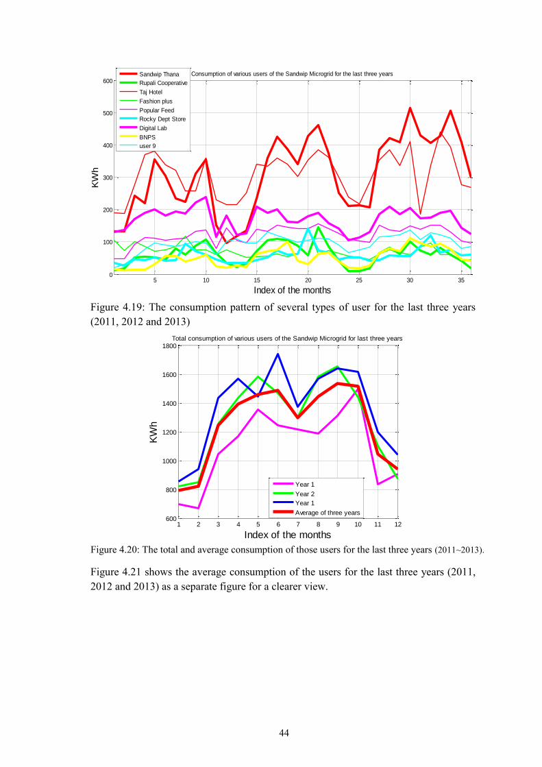
44

Figure 4.19: The consumption pattern of several types of user for the last three years (2011, 2012 and 2013)

Figure 4.20: The total and average consumption of those users for the last three years (2011~2013).

Figure 4.21 shows the average consumption of the users for the last three years (2011, 2012 and 2013) as a separate figure for a clearer view.

1 2 3 4 5 6 7 8 9 10 11 12600

800

1000

1200

1400

1600

1800

Index of the months

KW

h

Total consumption of various users of the Sandwip Microgrid for last three years

Year 1

Year 2

Year 1

Average of three years

5 10 15 20 25 30 350

100

200

300

400

500

600

Index of the months

KW

h

Consumption of various users of the Sandwip Microgrid for the last three years

Sandwip Thana

Rupali Cooperative

Taj Hotel

Fashion plus

Popular Feed

Rocky Dept Store

Digital Lab

BNPS

user 9

45

Figure 4.21: The average consumption of those users for the last three years (2011~2013).

This figure shows the approximate demand profile of 9 users of Sandwip microgrid. The actual demand profile is thus expected to be similar to Figure 4.21. Therefore, the actual demand of the microgrid will be a scaled-up version of Figure 4.21.

For avoiding complexity, the demand profile scaled up in such a way that it will have similar scale of figure 4.10 of previous analysis- around 6500KWh of consumption per month. As the scale of demand profile is similar to the previous analysis, the scale of the generation profile thus, would be similar to that of the previous analysis. 50KWp of Solar PV panel is being considered at this analysis like the previous one. The output of the panel at Sandwip for the default tilt is shown in Figure 4.22 as well as the demand profile. Figure 4.22 shows the scaled up representation of the average consumption of the users for the last three years (2011, 2012 and 2013) have a closer range of demand pattern like that of the national demand analysis.

Figure 4.22: The scaled up representation of Figure 4.21.

1 2 3 4 5 6 7 8 9 10 11 12700

800

900

1000

1100

1200

1300

1400

1500

1600

Index of the months

KW

h

Total consumption of various users of the Sandwip Microgrid for last three years


1 2 3 4 5 6 7 8 9 10 11 123000

3500

4000

4500

5000

5500

6000

6500

7000

Index of the months

KW

h

Total consumption(scaled up)of various users of the Sandwip Microgrid for last three years


46

The default tilt, optimum tilt, maximum generation of energy, maximum utilization of energy, random variation and the relationships among these have been discussed at the previous analysis. In the analysis of Sandwip, only the results are shown here. Figure 4.23 to Figure 4.28 show the results when the random variation is 0.01%, 0.1% , 1%, 2%, 5% and 10% respectively.

Figure 4.23: The number of maximum occurrence of minimum shortage for r=0.01% (tilt angle vs frequency of occurrences).

Figure 4.24 : The number of maximum occurrence of minimum shortage for r=0.1% (tilt angle vs frequency of occurrences).

0 5 10 15 20 250

50

100

150

200

250

Tilt Angle

Fre

quency


0 5 10 15 20 250

50

100

150

200

250

Tilt Angle

Fre

quency


47

Figure 4.25: The number of maximum occurrence of minimum shortage for r=1% (tilt angle vs Frequency of occurrences).


For 0.01%, 0.1%, 1% and 2% of the random variation, in most of the cases, the minimum shortage occurance appears at the tilt angle of 80 to 120 .

For larger variation of the demand and generation such as for r=5% and 10% the number of maximum occurance is still found to be around 70 and 130. These are shown in Figure 4.27 and Figure 4.28.

0 5 10 15 20 250

20

40

60

80

100

120

140

160

Tilt Angle

Fre

quency


0 5 10 15 20 250

50

100

150

Tilt Angle

Fre

quency


48

Figure 4.27 : The number of maximum occurrence of minimum shortage for r=5% (tilt angle vs Frequency of occurrences).


From the above analysis, it can be deduced that utilization of maximum power for a region may not be generated at a tilt angle of the default latitude. The default latitude will produce the maximum energy over the year, but maximum utilization of power will depend on tilt angle as well as the demand profile over the year. For a demand profile of microgrid in Sandwip and generation profile of Sandwip, the minimum shortage occurs for most of the time is at a tilt angle of 90 and around it. The demand, generation and surplus/shortage for default tilt (230) and optimum tilt (90) angles are shown in Figure 4.29.

0 5 10 15 20 250

10

20

30

40

50

60

70

80

90

Tilt Angle

Fre

quency


0 5 10 15 20 250

10

20

30

40

50

60

70

80

Tilt Angle

Fre

quency


49

Figure 4.29: The demand, generation and surplus/shortage for 230 and 90 tilt angle.

Though the difference in output is not significant in percentage between the default tilt angle and optimum tilt angle, the amount will be larger for a larger system. It is however be noted that the change of tilt angle will not maximize the output of the PV panel, rather, it will minimize the shortage and maximize the demand met. 4.12 Summary

For a country like Bangladesh, appropriate use of renewable energy resources is very important. To have a better life there is no alternative to providing sufficient electricity to all class of the population. Renewable energy, especially solar PV, is getting popular to mitigate the energy crisis of many countries. Mini grid or microgrid concurrent with SHSs can be much more effective and may be considered as a better solution to have power with quality, reliability and sustainability. In the next chapter, a novel algorithm has been proposed for optimization of the available distributed energy resources.

1 2 3 4 5 6 7 8 9 10 11 12-3000

-2000

-1000

0

1000

2000

3000

4000

5000

6000

7000

Index of Months

Dem

and,

Genera

tion,

Surp

lus o

r S

hort

age

Demand

Generation at 23 degree tilt angle

Generation around Optimum tilt angle

Surplus/Shirtage at 23 degree tilt angle

Surplus/Shirtage around Optimum tilt angle

50

CHAPTER 5

THE PROPOSED MODEL FOR DER BASED MICROGRID AND ITS IMPLEMENTATION

The last chapter described the analysis and optimization of the tilt angle of solar PV panel for a specific region. A comprehensive modeling of power generation in Bangladesh incorporating the available renewable energy resources, load demand profile and shortage/ surplus for various zones of Bangladesh has not been carried out in the past. As part of the current research, various relevant field data have been collected and appropriate mathematical models have been developed. This includes the analysis of electricity demand and its generation and optimization of the available resources, which are discussed in this chapter. 5.1 Analysis of Electricity Demand

The analysis of demand includes the yearly demand, seasonal variation of the demand and random variation of demand from the normal or average one. From the analyzed data of (sources: PGCB; last three years) it is found that the load profile follows almost a definite pattern. During the months from November to February of the year, the consumption of electricity is lower and the highest electricity consumption occurs at the month of July. Considering a number of 100 typical families of a village, the predicted/ average/ demand has been shown in Figure 5.1. In this prediction, it has been assumed that the load pattern follows that of the national grid, However, for a different load pattern, the analysis would be different.

Figure 5.1: Monthly predicted average demand for 100 number of typical village family.

1 2 3 4 5 6 7 8 9 10 11 120

1000

2000

3000

4000

5000

6000

7000

Index of months

Dem

and in K

Wh

Demand for typical 100 families of a remote area(kWh)

51

Figure 5.2 shows the demand and generation of the electricity for various sizes of solar PV panels and the corresponding shortage and surplus for the generation. It should be noted here that the shortage is decreasing with the increase of installed PV panels. However, reducing the shortage by installing higher energy resources is not a wise task. Hence, there should be an optimum size, where the surplus and shortage both would be minimum.

Figure 5.2: Demand, generation, shortage/surplus for various sizes of PV panels.

5.2 Analysis of the Generation

Like the demand of electricity, the generation of electricity also varies over the year depending on the availability of the energy resources. The renewable energy resources are intermittent sources. Thus, it renders long-term variation (seasonal) as well as short term (within a day) variation in its availability. Whatever be the resource- solar, wind, tidal or hydro, the generations of all individual resources vary with time. However, the resources have average generation capacity over the year. These renewable energy resources may be used to provide the power for the local inhabitants. 5.3 The Proposed Model for the DER Based Microgrid

The available microgrids are mainly a miniature of the traditional power system. That is, the electricity demand of an isolated area is supplied from a single centralized unit. In this model, single centralized generation unit is segmented as multiple smaller generation units of several renewable energy resources.

In the current research, it has been identified that proper sizing for the generation units to meet the demand is an important factor. It should be remembered that the pattern of yearly generation may not be same as the demand pattern. Shortage occurs when the demand is higher than the generation and surplus occurs when the generation is higher than the demand. Combination of several renewable energy resources with different

0 2 4 6 8 10 12-4000

-2000

0

2000

4000

6000

8000

Index of months

Dem

and,

Genera

tion,

Short

age/S

urp

lus(K

Wh)

Shortage or Surplus for various sizes

Demand

Generation for 40kWp



Shortage/Surplus for 40kWp



52

characteristics may help a particular power generation project to match the generation pattern with the demand pattern. To have an optimum model for a distributed energy based microgrid, the following major criteria have been considered to obtain the optimum result.

(i) Minimum shortage as well as unused energy(surplus) (ii) Maximum demand met

(iii) Minimum cost of the alternative sources (iv) Lower cost of energy (v) Higher penetration of renewable energy

(vi) Lower installation cost (vii) Lower running cost

5.3.1 Modelling of electricity demand and generation

As Bangladesh has several types of renewable energy resources that have already been discussed, analysis of combination of multiple resources to properly fulfill the demand is very important. To this end in view, an investigation has been carried out to formulate an appropriate mathematical model. Finally, the following important criteria/aspects have been adopted in developing and implementing the model:

(i) Determination of the probable demand/load pattern over the year (ii) Determination of per unit generation for each of the resources

considered. (iii) Determination of the total generation for several combinations of

multiple resources with multiple numbers of units. (iv) Determination of the generation pattern for the combined resources. (v) Determination of surplus or shortage over the year.

(vi) Searching the minimum shortage, where the demand met is maximum and the price of alternative energy resources (such as fuel-based generator) to meet the shortage is minimum.

(vii) Determination of the combination, where the cost of energy is minimum.

(viii) Determination of the combination, where the penetration of renewable energy is the highest.

(ix) For an analysis closer to the real scenario, a random variation to the monthly/daily demand and generation has to be considered.

It should be noted here that the analysis may be of two types: simple analysis and analysis that includes random variation in demand and generation.

(a) Simple Analysis

Here, demand is denoted by D. Monthly Demand over the year is D1, D2, … … … … … …, D12 (load profile). Similarly generation is denoted by G and monthly total generation over the year is G1, G2, … … … … … G12 (generation profile). Shortage will occur for D>G and surplus when D<G surplus.

53

(b) Analysis Including the Random Variation

In this analysis it has been assumed that both demand and generation vary randomly for various real time causes. The demand is assumed to vary between +r% to –r% and average demands for several months are D1a, D2a, D3a, … … … D12a, where „D‟ stands for demand, the number after D is the index of the months and „a‟ stand for average. The daily demand of a month can be predicted from the average monthly demand including the random variation in it. This is shown in equations 5.1 and 5.2.

For January (D1): The number inside “( )” after Dn represents the particular day of the month.

D1(1) = D1a*[(100-r)+ 2*r*rand()]% … … … … … … (5.1.1) D1(2) = D1a*[(100-r)+ 2*r*rand()]% … … … … … … (5.1.2)

. . . . . . . . .

. . . . . . . . .

. . . . . . . . .

. . . . . . . . .

D1(31) = D1a*[(100-r)+ 2*r*rand()]% … … … … … … (5.1.31)

A generalized formula can be expressed as Dn(x) = Dna*[(100-r)+ 2*r*rand()]% … … … … … … … (5.2)

Similarly, the prediction of generation for a resource may be expresses as Gn(x) = Gna*[(100-r)+ 2*r*rand()]%… … … … … … … (5.3)

where, „n‟ denotes the index of a month „x‟ denotes the xth day of a month „a‟ indicates the average „r‟ is the probable variation of demand or generation „rand()‟ produces a random value that is greater than 0 and less than 1.

As, there are several types of energy resources, the total generation will be the summation of all the generations as follows:

GTn(x) = G1n(x) + G2n(x) + -------------- + Gmn(x) … … … … … (5.4) where, GTn(x) = daily total generation by all of the resources for month of n G1n(x) = daily generation by resources 1 for month of n G2n(x) = daily generation by resources 2 for month of n Gmn(x) = daily generation by resources m for month of n

Thus, the demand and generation for each individual day can be randomly predicted using equations (5.2) and (5.3). This will provide closer view of a realistic demand and generation scenario. However, variation of demand and generation could also be predicted in a similar way on top of the monthly data (Figure 5.1 and Figure 5.2) easily, which would provide a crude approximation of the variation, but has not been used here.

54

It is expected and logical that the combination of several types of renewable energy resources will best fit the generation profile with the demand profile. The calculation of the analysis has been incorporated using the MATLAB programming environment. The MATLAB implementation routine is included in Appendix-D. 5.4 Optimization of the Resources

There may be multiple numbers of resources. This model is a general model in which combination of several types of resources could be analyzed. Considering N1 number of size for resource R1, N2 number of size for resource R2, and Nm number of size for resource Rm will have Ntotal number of different combination of resources.

Where, Ntotal= N1 x N2 x N3 … … … x Nm --- --- --- --- --- (5.5)

The analysis has been done based on this idea. Due to the enormous size of combinations and thus a huge amount of data to be handled, the analysis of only a single resource has been discussed in this chapter.

An optimized design does not necessarily provide a unique result. The basis of optimization is an important factor, such as optimization for minimum production cost per unit, minimum installation cost, maximum penetration of renewable energy, minimum cost for alternative energy resources, etc. Change in the basis of optimization will change the result. An optimum design for minimum shortage does not mean the optimum design for minimum production cost or so. Among the several types of optimization, Figure 5.3 shows the result for optimum size of PV panel that has to be installed for minimum shortage and minimum surplus.

Figure 5.3: The optimum scale of the solar PV for minimum shortage and minimum surplus.

0 10 20 30 40 50 60 70 800

2

4

6

8

10

12x 10

4

Installed Capacity

Short

age o

r S

urp

lus

Installed Capacity VS Shortage or Surplus for Optimum Size

Demand

Generation

Demand met

Shortage

Surplus

Difference bet Shortage and surplus

55

To design the project properly, the following criteria should be taken into consideration:

(i) Utilization of the surplus (ii) Back up for the shortage

(iii) Maximize the penetration of renewable energy (iv) Ensure the minimum cost of energy (v) Minimum utilization of the fuel-based generator

(vi) Minimum shortage (vii) Minimum surplus

(viii) Minimize the unused energy (ix) Cost of the fuel based energy to meet the shortage. (x) If the surplus is kept zero that is all energy generated is consumed

then the shortage will be maximum thus the cost of extra energy will be maximum.

(xi) If the shortage is to be zero, surplus will be maximum and the installation cost will be higher.

An optimization algorithm has been formulated where the above criteria have been taken into consideration. This algorithm has been implemented using MATLAB programming environment and included in Appendix-D. The results of the analysis of demand and generation as well as the optimization algorithm will be discussed in chapter 7.

To show how the model works, only one energy resource (solar PV alone) has been considered to obtain the output in this chapter. However, solar, biogas, wind, diesel hybrid system has also been analyzed in the same way and the MATLAB program is included in appendix-D. The results of this analysis is shown in Appendix-E 5.5 Summary

The proposed model for the analyses of demand and generation and the algorithm for optimum use of the available distributed energy resources have been discussed in this chapter. In the next chapter, a realistic and reliable design model for optimum utilization of the DER based microgrid will be presented.

56

CHAPTER 6

CONSUMER IS PRODUCER - A NOVEL MODEL FOR ELECTRICITY GENERATION

Chapter five described the proposed algorithm to optimize the available distributed energy resources. This chapter explores a new model to generate electricity with higher penetration rate of renewable energy. Conventional system to generate electricity is to generate large amount electricity and it reaches to the consumer through a long transmission line and distribution system. The losses and costs, incorporated with these processes, are not negligible. Another System is the Solar Home System (SHS), which has been used in Bangladesh from 1998 to replace the traditional kerosene based lamp and enable the use of battery based TV, DC fans and light bulbs. With the advancement of technology, the energy demand of the consumers is increasing significantly. To meet this demand, it needs connectivity to the national grid. An alternative to this is to produce enough power at the consuming spot. A novel method to achieve this has been discussed in this chapter. A brief overview of the power sector of Bangladesh and some of the topics discussed in the previous chapters have been repeated here for convenience. Also, the performance of the proposed system has been compared with that of the traditional power system.

6.1 A Short Overview of the Power Sector of Bangladesh

Bangladesh is a small country with a large population and the generation of electricity is not enough to serve the population. Presently, 62% [1] of the total population (including renewable energy) has access to electricity and per capita generation is 321 kWh, which is very low compared to other developing countries. Along with the centralized generation, till April 2014, about 3 million SHSs have already been installed in the off-grid rural areas of Bangladesh under the program run by IDCOL with co-operation of several other supporting agencies. As a result, more than 13 million beneficiaries are getting solar electricity, which is around 10% of the total population of Bangladesh. Most of the installed units of SHS are used at homes. A few of them are used in educational institutes, prayer houses and shops in the market. A solar home system is able to provide electricity for a few light bulbs, small DC fan and TV, rechargeable torch light, adapter for mobile phone charging etc.

However, the energy demand of the customer is increasing significantly. Many of the customers have intention to use a large TV, fridge, electric iron, blender, domestic water pump even AC, like a customer having connection of national grid electricity. However, extension of the grid is not an easy task. Besides this, most of the power stations is based on natural gas which is about 78.12% of the total capacity on the FY 2013 [1]. On the other hand, natural gas is on short supply and about 1500 MW of generation

57

shortfall occurs due to shortage of gas [15]. Therefore, it will be very tough to provide more electricity generated from the natural gas in future. Government of Bangladesh is trying for some alternative of natural gas such as coal, HSD, Furnace oil based power plant as the fuel diversification program [1][2]. Presently, use of gas, HSD, Coal and FO are around 80%, 10%, 5%, 3% respectively [15] of the total generation. On the other hand, Bangladesh naturally receives plenty of solar radiation from the sun. Wind, mini hydro and micro hydro are also available and there is scope to solve the problem of electricity generation with the combination of several renewable energy resources with storage and non-renewable fuel-based generation units. 6.2 Field Survey

A field study has been carried out on several customers of the existing SHSs including the area of Jessore, Rangpur, Laksmipur, Mymensingh, Sandwip, Hatia and Vola from November 2012 to August 2014. It is found that many of the remote areas are yet far from the national grid. In those areas, most of the inhabitants use kerosene lamps/lanterns for lighting purposes. Some of them are using diesel or petrol-based electrical generators in groups for a limited period of the day due to higher fuel cost. SHS is also being used in this area. SHS system is primarily design for lighting purposes. It can also provide energy to TV and low power DC fans. The users of current SHS are interested to use standard TV, fridge, fan, small water pump etc. However, due to lack of enough power, they cannot use these appliances. An alternative way to meet their demand and to provide the similar service as the national grid does, is to produce enough power at the consuming spot and interconnect them locally. This study also shows that a typical house at a village area (nearest to an electrified village) consumes about 50 kWh of electrical energy per month. The average free space of roof is about 40-50 m2

and the average usable space for solar PV application is about 18-25 m2 whether the roof is South (or North) faced or East (or West) faced for a slopped rooftop. For a flat roof, the complete roof area may be used. This area is enough to install solar PV of more than 2-3kWp capacity. It will produce about 210-450 kWh of usable electricity per month, which is enough for 3-5 families of a village, considering the consumption pattern of a traditional family. 6.3 Scopes of Interconnected Microgrids

A conventional power system usually consists of large scale power stations, transmission lines, substations and distribution lines etc., where the generation and consumption of power are not at the same location. By this system, remote areas are normally not connected with the electricity grid, and thus are deprived from development to take place. The traditional power system is also associated with transmission and distribution losses, environment pollution, higher installation cost as well as running cost. Moreover, the load management system also hampers a large number of users. Using the available resources in a remote area, the output of each source of energy i.e. solar PV, biogas, wind etc. may be interconnected locally, and thus this interconnected system will provide enough electrical energy for the entire user

58

of the locality by means of Micro-grid [7]-[9]. The idea of microgrid and DER is being used in several countries in a larger scale. The penetration of DER based microgrid is increasing in the developing country day by day. A Revolution of the microgrid can solve the power crisis of the world in an easier way.

Considering the points above, a new model for generation and distribution of electricity has been proposed. It is expected that the implementation of this model will ensure less transmission and distribution loss and the cost will also be minimized significantly, emission of CO2 will be negligible with a new load management technique as well as ensuring reliable and quality power within the shortest possible time. 6.4 Consumer is Producer - an Alternative Approach [1]

[2] Consumer is Producer (CP) model is a new technique to generate and distribute electricity with higher power quality, stability, reliability, lower transmission and distribution loss and the overall lower cost to produce electricity. It is designed as easier as plug and play equipment. It will be able to provide electricity to a large number of populations within the shortest possible time. [3]

Before discussing the model, the topology of several layers of the model of the microgird should be clarified at first. In this context, Figure 3.7 and Figure 3.9 are recalling here.

Figure 6.1: Recalling Figure 3.7 and Figure 3.9.

Figure 3.7 is the traditional microgrid, where there is no transmission line, rather user level distribution is present only and the generation of power is centralized and Figure 3.9 is the proposed microgrid, which is similar to the traditional microgrid but power generation is distributed over the entire area.

Generation is shown by red rings, blue rings represent the low voltage level distribution and the green rings represent the consumers. To show the generation and the consumption at the same place, the red and the green rings are merged by both of the colors. This is shown in Figure 6.2.

59

Figure 6.2: Ring diagram of a new microgrid model, where the generation and consumption will take place at the same point.

In the proposed model, generation and consumption will take place at same point. And the distribution line will be used to share the power to several users as well as proper management of the microgrid. Thus the layers of the microgrid may be expressed by Figure 6.3.

Figure 6.3: Several layers of the proposed microgrid, where closeness of the rings shows the integrity of generation and consumption.

Instead of using two different rings for showing the generation and consumption, single ring has been used to express the idea in Figure 6.4. As the name implies, this ring may be called the layer for consumer-producer units.

60

Figure 6.4: Two different rings expressing the consumer and producer units have been merged into a single ring keeping the distribution close to the generation and consumption.

This type of microgrid may form in several places of remote areas of a country. In this case, interconnection among the microgrids will be possible. Development of microgrids in several places is shown in Figure 6.5.

Figure 6.5: Discretely developed microgrids, may be interconnected.

[4] So far, the topology of the proposed microgrid has been discussed. The layers of the model comprises with Consumer Producer Unit (CPU), microgrid, interconnected microgrid, and control and management unit. Brief descriptions of these are given below. [5] 6.4.1 CPU [6]

[7] The unit CPU (Figure 6.6) consists of source or sources, loads, control and management system in a unit. Each CPU has its unique identification number.

61

[8] [9]

Figure 6.6: Block diagram of Consumer Producer Unit (CPU). [10]

[11] Sources: The sources may be solar PV, biogas based-generator, small wind generator, small hydro power generator, fuel cell, micro-turbine, gas or diesel generator or any storage element such as battery, fly wheel etc. [12]

[13] Inverter: Whatever be the output of the sources is, the output of the inverter will be AC. Inverter output is kept same as that of the grid. [14]

[15] Synchronizer: The task of the synchronizer is to synchronize the output of the inverter with another CPU or with the grid. [16]

[17] Communication module: The task of this module is to communicate with a Master controller or central controller about the status of the CPU. It receives command from the central controller and executes the command such as to disconnect any load, disconnect itself or disconnect sources (for example, diesel generator was running over the night and at the day time central controller accumulates the data of all of the CPU and decides that, now there is no need to run the diesel generator, then it will send command to the CPU of the diesel generator to stop it.) [18]

[19] Energy meter: It measures the amount of generated or consumed energy; calculate the bills for peak time, off peak time, demand charges etc. Energy calculation module calculates the energy incoming from the grid, outgoing to the grid and the amount of energy used by the loads. [20]

[21] Loads: The loads of the consumer is categorized for a better load management, such as lighting load, fan load, refrigerator, TV, computer, and heavy loads like AC, pump etc. [22]

6.4.2 Microgrid [23]

[24] The microgrid is an inter connection of several numbers of CPUs. The formation of a microgrid by several CPUs is shown in Figure 6.7. This is an alternate expression of Figure 6.4

62

[25] [26]

[27] Figure 6.7: CPU based Microgrid. [28]

6.4.3 Interconnected Microgrid [29]

[30] Interconnection of several microgrids may be achieved by using central controller as shown in Figure 6.8. This is an alternate expression of Figure 6.5. However, interconnections of microgirds have not been shown in Figure 6.5. [31]

[32] [33]

[34] Figure 6.8: Interconnection of Microgrid with central controller. [35] 6.4.4 Microgrid Network [36]

[37] When a large number of interconnected microgrids are combined together, it will form a microgrid network. The microgrid network may be considered as a unit power source that will be connected to the nearest transmission and distribution lines. This is shown in Figure 6.9.

63

[38] [39]

[40] Figure 6.9: Microgrid Network. [41]

6.4.5 Connection to national grid [42]

[43] An option has been provisioned for it to be connected to the nearest national grid when available. Through this connection, it is possible to transfer power to the grid on demand. This is shown in Figure 6.10. [44]

[45] [46]

[47] Figure 6.10: Microgrid connected to national grid. [48] 6.5 Control and Load Management [49]

[50] The control of voltage, frequency, real and reactive power, droop4 etc. can be controlled by the central controller of the interconnected microgrid. It will control the frequency, voltage and other parameters to ensure better quality of power. Like the central controller, each of the CPU has its own identification number. Each central controller will be connected to some branches of a microgrid, but it will control only a few of the branches which are defined to be controlled under it. As the loads are categorized, the central controller will send command to disconnect some types of load when generation is less than the demand. Under this circumstance, the traditional method is to disconnect the branch completely, and as a result, a large number of consumers are affected.

4 Sloop of frequency vs power

64

[51] 6.6 Determination of Maximum Voltage Between Two Isolated Microgrids

when Interconnected

The energy resources are distributed (Figure 6.7) over the microgrid (proposed) instead of central power generation. For such a system, the loads and the resources may be expressed by the thevenin equivalent circuit. Figure 6.11 is expressing the thevenin diagram of an isolated microgrid.

Figure 6.11: Two CPU based isolated microgrid are expressed by equivalent thevenin circuit.

The interconnection of these two microgrid may be done by connecting node 1 and node 2. This connection is used for transferring power from one microgrid to another. Thus the characteristics/parameters of this line could be found out through a similar as that of transmission line. This line may be expressed as by Figure 6.12 and Figure 6.13 with a combination of an equivalent resistance, inductance and capacitance [29].

Figure 6.12: Resistance, Inductance and capacitance of the line and equivalent.

Here, R1, R2… Rn denotes the resistance of the various segments of the line and L1, L2… Ln denotes the inductance of the various segments of the line.

Figure 6.13: Capacitance of the line and its equivalent.

65

There will be a voltage drop between the nodes only if there is any current flow through the line and thus power transfer. In such a case one node will deliver power to the other node. Therefore, one node could be assumed as a source and another could be as load. The complete equivalent circuit may be expressed by a combination of equivalent source, resistance, inductance, capacitance and load [29]. This is shown in Figure 6.14

Figure 6.14: Equivalent circuit of the inter-connection line. The parameters could be found by analyzing the characteristics of the conductors. The inter-connection line is nothing but a low voltage level distribution line. Typical distribution line characteristics [29] are given below:

Conductor characteristics

Single phase Cable: Aluminum Length =1km Radius of the conductor=1cm Distance between the conductor = 0.5m=50cm Resistivity of conductor at 200C, ρ = 28.2 nΩ-m Cross sectional area, A=πr2 =π x 10-4

The inductance of line per m could be found by this equation The resistance, inductance and capacitance could be found by the equations 6.1 to 6.3. However, as there are two conductors, the total resistance will be double of R. Resistance of line,

R= ρl/A ……………..(6.1) Loop inductance per meter,

L= 10-7

H/m……………..(6.2)

Capacitance per meter,

C

(

)…………………(6.3)

66

Inductance and capacitance for per km of line could be found by multiplying this value by 1000. From the value of L and C, inductive reactance and capacitive reactance could be found by equations 6.4 to 6.5. Inductive reactance,

XL= 2πfL ………………….(6.4) Capacitive reactance

XL= 1/2πfC………………….(6.5)

The microgrid is small and isolated. Assuming a total 10KW load being served in a microgrid by another, the is Standard impedance for 10KW load with power factor 0.8 This information are incorporated in a MATLAB file which is given in Appendix –F and output of program is shown in Figure 6.15. It is found that the voltage drop increases with the length of the interconnection line.

Figure 6.15: Voltage drop vs distance of interconnection.

The Figure shows that the voltage is around 210V for a distance of 300 meter. Therefore, three or more CPU may be inserted into the interconnection line to reduce the distance around 300 meters instead of 1000 meters. 6.7 An Applicable Implementation Policy

The proposed scheme is a new model and hence it needs appropriate policy to be incorporated. Policy is an important factor for any program. There may be several entities to form the proposed microgrid. The users may form a microgrid by interconnecting their own CPUs. However, this will create problem if there is no policy for interconnection in the local grid. Without any controlling entity over the grid, it will be more complicated to implement this scheme. Therefore, it is better for a new entity to be connected into an already formed microgrid. For a better explanation of the problem, let us assume that entity 1 will provide the connectivity to the local microgrid for any new entity. Entity 1 will be responsible for

100 200 300 400 500 600 700 800 900 10000

50

100

150

200

250

Distance of Node 2 from Node 1

Voltage

Distance Vs Voltage drop and Voltage at Node 2

Voltage Drop in Interconnection line

VOltage at Node 2

67

the generation, grid related hardware and software support and the backup power. It will have its own power as well as buy power from entity 2. Entity 2 will be responsible for generation, backup (in some cases) and consumption. There may be a third type of entity namely, entity 3, which would be responsible for consumption only. Suppose that all of the power generated by entity 2 will now be sold to entity 1 with a price of B Tk./unit and entity 1 will sale this power to entity 2/entity 3 with a price of S Tk./unit.

As renewable energy resources are intermittent sources, there must be a backup power or storage of energy to have a reliable and continuous power supply. If anyone of entity 2 wishes to stay disconnected from the grid and have a smooth and reliable operation, he must have additional backup power and generation. Thus, it will cost 3~5 time more than the cost if connected with the grid. In this case, the return of initial capital will be delayed; actually, there will be no return, instead there will be a saving of cost of energy. Therefore, it is better to be connected with the grid, as it will reduce the initial investment and ensure the reliable and continuous supply of power.

For individual use, the day of autonomy is important. Day of autonomy is defined as the number of days in which the system will be able to operate without any interruption. It is kept as three days as standard. This is done by storing the energy into deep cycle batteries. This costs a huge portion of the initial cost. Presently, market price of 100Wp panel is about 6,000Tk. and the battery used to store the energy of the panel for 3 days autonomy (150Ah-12V), which costs about 18,000Tk. There are also costs for wiring, structure, controller and labor. By these ways, it will cost around 300Tk. per Wp to be installed. The market price of an SHS without inverter is about 40,0000Tk. Thus initial cost will be around 400Tk per Wp of solar panel.

In the case of grid connected mode, the cost is associated with only the panel, controller (here CPU), structure and labor. There is no cost for the storage. The approximate cost for the CPU may be 40,000Tk. for a 2KWp capacity panel. Including other costs such as labors, cable etc., the total cost to install a 2KWp capacity PV panel will be around 1,20,000Tk. In this way, it will cost around 90Tk. to install 1Wp of solar panel. However, in this mode, cost for backup energy whether it is by means of battery or fuel based generator, will solely be borne by entity 1. It is to be noticed that the backup of the power may be accomplished by using battery only or by using fuel based generator with battery. For individual use, whether the backup energy is by means of battery (3 days autonomy needs a battery of large size) or by means of battery with fuel based generator, it will make the cost higher for entity 1 whereas, the cost will be lower for the grid connected mode as it is a large system.

On the other hand, the day autonomy for a grid is not three days rather the autonomy is for the period of sun set to sun rise (actually the period of zero production to start of production by the solar panels). For this reason, the size of the battery needed for the grid connected mode is just enough to store 40% of the total energy produced by the PV panels (like Sandwip Microgrid). Moreover, additional cost will be needed for the generator to run on the fuel. As a result, the cost associated for backup power or

68

alternative energy for the grid connected mode would be much less than that for the individual mode. However, the running cost will increase slightly. Other cost associated with entity 1 is for the poles, cables, controllers for the distribution system.

For a clear understanding, the discussion may further be divided into two stages; namely, stage 1: for building the grid backbone and a few of the power sources, which are related to entity 1, and stage 2: for interconnection of new CPUs to the existing grid, which is related to entity 2. Let us calculate the cost for a 100KWp solar microgrid (CP model) with the help of these stages.

6.7.1 Stage 1: Building the grid backbone and a few of the power sources

In this stage entity 1 will all the requirements that have already been discussed for the grid backbone so that entity 2 / entity 3 can easily connect their CPUs when they wish. Power generated by entity 1 and entity 2 will be available in the grid to be consumed. Approximate cost for the stage 1 is given the table below. It is assumed that initially demand as well as the number of connected CPUs will be less than that of saturated grid. Let, the total connected solar panel by entity 1 is SP1 and by entity 2 is SP1. In this case, the total connected CPUs in the grid will be SPT. Battery needed for this size of solar panel is BT (Sandwip) whether it is served by entity 1 or by entity 2. For easy calculation, it is assumed that the total battery needed will be installed by entity 1. Also a fuel based generator is needed for a reliable operation. The size of the backup generator will depend on the maximum demand of the system.

Presently, 40 customers are connected to the grid per km of distribution line (PDB and PBS data). For 200 users (types 2 and type 3), it needs 5km distribution line and 1km for interconnections of the line. The number of distribution pole is around 60 (1 pole per 100 m). There are also cost involvements for central controllers and others equipment.

6.7.2 Stage 2: Interconnection of new CPU to the grid

It was mentioned previously that, the free space of rooftop a typical village is enough to install 2KWp of solar panel. In this case, there will be no additional cost for the land. The associated cost is given in Table 6.1.

Table 6.1: Initial investment for entity 1

Components Size Price Breakdown Total BDT Panel 10KWp 10,000*60=6,00,000 6,00,000 Battery 48000Ah, 12V 5 48,00,000 Distribution System 5km 5km*80,000=4,00,000 4,00,000 Distribution Pole 60 60*10000 6,00,000 Diesel 10KW Generator 3 2,00,00*3 6,00,000 Control Equipment 1,00,000 Others (Land, labor, transport etc.)

10,000 per KWp 1,00,000

Total 70,00,000

5 Size of Battery is determined from the data of Sandwip 100KWp Microgrid

69

Installation cost for entity 1 may be given by

CT1= CP +CB+CDL +CDP+CFG+ CCE+Co … … … … … (6.1) where,

CP1= Cost for solar panel CB= Cost for Battery backup CDL= Cost for Distribution lines CDL= Cost for Distribution poles CFG= Cost for fuel based generator CCE= Cost for Control equipment CO= Other costs (labor, land transport etc.) CT1=Total Cost.

The Per Year Calculation for Entity 1 is given in Table 6.2

Table 6.2: Per year calculation for entity 1

Item Notation Amount in KWh

Unit price

Tk./KWh

Total cost (Tk.)

Usable energy from the Panel per year (entity 1)

EP1 13,000

Total energy buy from entity 2 (90KWp) 56,00,000 Tk.

EP2 1,17,000 20 (B) 23,40,000 (CB2)

Total Energy from Panel EPT= EP1+ EP2 1,30,000 Energy loss due to battery (Charging and discharging)

EPL 5,2006

Energy used from Panel EPU= EPT - EPL 1,24,800 Energy from DG ( Assume 30% of Total) EDG 53,485 15 7 8,02,285 (CDG) Total Energy sell ETS = EPU + EDG 1,78,285 25 (S) 44,57,142 (TS) Yearly Running Cost (employee + other cost)

4,00,000 (CR)

Cost per year 35,42,000 TC= CB2+CDG +CR

Net Profit per year 9,15,142 TP=TS - TC

The total Energy sale may be given by,

TS1= (EP1+ EP2 - EPL + EDG)*S … … … … … … (6.2) The total cost per year is given by,

TC1= EP2*B+CDG +CR1 … … … … … … … (6.3) 6 5% of the total generation by solar

7 Energy cost by Diesel Generator is assumed same as Sandwip 100KWp Microgrid

70

And the net profit per year is given by, TP= TS - TC… … … … … … … (6.4)

where, Usable energy from the Panels of entity 1per year = EP1 Total energy buy from entity 2 (Total 90KWp) = EP2 Total Energy from Panel, EPT= EP1+ EP2 Energy loss due to battery (Charging and discharging) =EPL Energy used from Panel, EPU = EPT - EPL

Energy from DG (Assume 30% of Total)= EDG

Yearly Running Cost (employee + other maintenance cost)= CR1

Initial investment for Entity 2 is given in Table 6.3.

Table 6.3: Initial investment for Entity 2

Components Notation Size Price Breakdown Total Panel CP1 2KWp 2,000*60=6,00,000 1,20,000 CPU CCPU 20,000 per

KWp 40,000

Others CO 20,000 Total CT2 1,80,000

The installation cost for entity 2 is given by CT2= CP2 + CCPU + Co … … … … … (6.5)

where, CP2= Cost for solar panel by entity 2 CCPU= Cost for CPU Co= Other costs

Yearly cost calculation for entity 2 is given in Table 6.4

Table 6.4: Yearly cost calculation for entity 2

Item Total energy sale Unit price of energy Total Usable energy from the Panel per year

2600KWh Selling price 20 52,000

Running cost 2% of initial cost 3,200 Net Profit per year 47,800

Yearly Running Cost (employee + other maintenance cost)= CR

The total Energy sale may be expressed as

TS2= EP2*B … … … … … … (6.6) The total cost per year is given by,

TC2=CR2 … … … … … … … (6.7)

71

And the net profit per year is given by, TP2= TS2 - TC2… … … … … … … (6.8)

Further increase of demand may be met by adding more solar panels by entity 2. This may require additional storage or backup. This storage/backup service may be incorporated by the entity 1 or by the entity 2. Results of these analyses are included in chapter 7. 6.8 Summary

The proposed model can be used as an alternative and supplement to the traditional power systems. As the scale of the unit is assumed to be smaller than the unit of a traditional large renewable energy microgrid, but larger than the unit of a solar home system, this will penetrate a significant percentage of renewable energy into the national generation. Due to its easy installation and maintenance, it will require less installation time and thus would allow a quicker growth of penetration of renewable energy into national energy production. It is logical that this inrush will unlock the power market for the common people. Besides these, the rate of global warming will decrease. The various components of the proposed model have been described in this chapter as well as an relevant example of policy description to implement this model. The features of this model, along with the policy, analyses of economic feasibility and projection of the installed capacity will be discussed at the next chapter as well as the results obtained from the analysis described in Chapter 4, Chapter 5 and Chapter 6 using the developed software routines.

72

CHAPTER 7

RESULTS AND DISCUSSION

In chapter 4, the tilt angle of the solar panels has been optimized to generate electricity to match with a specific load demand pattern. Analyses of the demand and generation of electricity by using the distributed` energy resources in a local microgrid have been proposed and the implementation process has been discussed in chapter 5. Finally, considering the overall aspects of electricity generation, distributed energy resources and the quick penetration of renewable energy resources in power generation, a novel model named “Consumer is Producer” has been proposed and described in chapter 6. This chapter will present the results of the three major propositions (in Chapter 4, Chapter 5 and Chapter 6) and discuss the results in a greater detail. 7.1 The Tilt Angle Optimization of Solar Panels and Its Benefits

In this analysis, it is found that, the maximum demand for an isolated grid is not met at the default tilt angle of solar panel; rather, it depends on the demand pattern as well as the generation pattern. Our demand is higher in July and around it and lower at November to February of a year. However, the generation of solar PV is not same as the demand pattern. The idea about the best matching pattern of generation at different tilt angles with the demand profile could be best comprehended from their correlation co-efficients. These are shown in the Table 7.1

Table 7.1: The correlation co-efficient (CC) of generation at Dhaka with national demand profile and generation at Chittagong with Sandwip microgrid demand profile.

From Table 7.1, it is found that, at the default tilt angle (230), the co-efficient is negative, thus there is a bad pattern match. Decreasing the tilt angle will results a better co-efficient and thus a better pattern match of demand and generation. On the other hand, total yearly output will decrease when the tilt position is shifted from default. In this case, 50 tilt angle may not provide the power to maximize the demand met although it has a better CC.

Tilt

A

ngle

50 60 70 80 90 10

0 11

0 12

0 13

0 14

0 15

0 16

0 17

0 18

0 19

0 20

0 21

0 22

0 23

0 24

0 25

0 26

0 27

0 28

0

CC

(D

haka

)

0.15

9 0.

111

0.06

2 0.

012

-0.0

37

-0.0

87

-0.1

36

-0.1

82

-0.2

28

-0.2

71

-0.3

12

-0.3

52

-0.3

88

-0.4

21

-0.4

52

-0.4

80

-0.5

06

-0.5

30

-0.5

51

-0.5

71

0.58

9 -0

.605

-0

.620

-0

.634

CC

(S

nadw

ip)

0.15

6 0.

103

0.04

8 -0

.009

-0

.068

-0

.127

-0

.186

-0

.244

-0

.301

-0

.355

-0

.406

-0

.454

-0

.497

-0

.537

-0

.574

-0

.607

-0

.637

-0

.664

-0

.689

-0

.711

-0

.731

-0

.748

-0

.764

-0

.778

73

The analyses have been done for both of the national demand profile considering the generation profile of Dhaka and for the demand profile of the newly formed microgrid at Sandwip considering the generation profile of Chittagong (nearest observation point to Sandwip by NREL).

Demand and generation for the default tilt angle (230) and optimum tilt angle (120) for the national load profile have been shown in Figure 7.1.

Figure 7.1: Demand and generation for the default tilt angle (230) and optimum tilt angle (120) -case study Dhaka.

From the above figure, it can be noted that, the demand is higher from the June to October over the year. At this period, the demand cannot be met by the solar panel, alternate resources of energy is needed. However, the curve for the optimum tilt is closer to the demand curve than that for the default tilt angle. Thus the demand met at optimum tilt will be more than that at default tilt. These are shown in Figure 7.2.

Figure 7.2: Demand met for default and optimum tilt angle-case study Dhaka.

As the demand cannot be met by panel for a period over the year, there would be shortage at that period. Shortage will be less for the optimum tilt. This is shown in Figure 7.3

1 2 3 4 5 6 7 8 9 10 11 124000

4500

5000

5500

6000

6500

Index of Months

KW

h

Demand and Generation for default and optimum tilt angle-DHK

Demand

Generation at Default Tilt

Generation at Optimum Tilt

1 2 3 4 5 6 7 8 9 10 11 124000

4500

5000

5500

Index of Months

KW

h

Demand met for default and optimum tilt angle-DHK

Demand met at Default Tilt

Demand met at Optimum Tilt

74

Figure 7.3: Shortage at default tilt and optimum tilt angle position- case study Dhaka.

The results are summarised in numerical figures as follows:

(a) Yearly total demand: 62,950 KWh (b) Yearly total Generation at 230 tilt angle: 63,158KWh (c) Yearly total Generation at 120 tilt angle: 61,705 KWh (d) Yearly total shortage at 230 tilt angle: 5,910 KWh (e) Yearly total shortage at 120 tilt angle: 5,400 KWh (f) Yearly demand met 230 tilt angle: 57,040 KWh (g) Yearly demand met 120 tilt angle: 57,550 KWh

The result of the analysis for the demand profile of the microgrid of Sandwip and considering the generation profile of Chittagong is given here. The tilt optimum angle for this case is found around 90 tilt. Demand and generation for the default tilt angle (230) and optimum tilt angle (90) for the national load profile have been shown in Figure 7.4.

Figure 7.4: Demand and generation for the default tilt angle (230) and optimum tilt angle (90)-case study Sandwip.

1 2 3 4 5 6 7 8 9 10 11 12-2500

-2000

-1500

-1000

-500

0

Index of Months

KW

h

Shortage for default and optimum tilt angle-DHK

Shortage met at Default Tilt

Shortage met at Optimum Tilt

1 2 3 4 5 6 7 8 9 10 11 123000

3500

4000

4500

5000

5500

6000

6500

7000

Index of Months

KW

h

Demand and Generation for default and optimum tilt angle-Sandwip

Demand

Generation at Default Tilt

Generation at Optimum Tilt

75

It is also true for Sandwip microgrid that, the demand is higher from the May to October over the year. At this period, the demand cannot be met by the solar panel, alternate resources of energy is needed. However, the curve for the optimum tilt is closer to the demand curve than that for the default tilt angle. Thus the demand met at optimum tilt will be more than that at default tilt. These are shown in Figure 7.5.

Figure 7.5: Demand met for optimum and default tilt angle-case study Sandwip.

As the demand cannot be met by solar panel for a period over the year, there would be shortage at that period. Shortage will be less for the optimum tilt. This is shown in Figure 7.6

Figure 7.6: Shortage at default tilt and optimum tilt angle-case study Sandwip.

The results are summarised in numerical figures as follows:

(a) Yearly total demand: 63,641 KWh (b) Yearly total Generation at 230 tilt angle: 66,244 KWh (c) Yearly total Generation at 90 tilt angle: 63,844 KWh (d) Yearly total shortage at 230 tilt angle: 70,95.5 KWh (e) Yearly total shortage at 90 tilt angle: 64,14KWh (f) Yearly demand met 230 tilt angle: 56,546KWh (g) Yearly demand met 90 tilt angle: 57,227KWh

1 2 3 4 5 6 7 8 9 10 11 123000

3500

4000

4500

5000

5500

6000

6500

Index of Months

KW

h

Demand met for default and optimum tilt angle-Sandwip

Demand met at Default Tilt

Demand met at Optimum Tilt

1 2 3 4 5 6 7 8 9 10 11 12-1800

-1600

-1400

-1200

-1000

-800

-600

-400

-200

0

Index of Months

KW

h

Shortage for default and optimum tilt angle-Sandwip

Shortage met at Default Tilt

Shortage met at Optimum Tilt

76

7.2 Sizing of Generation for Various DERs

Analysis of the demand and generation of electricity by using several distributed energy resources (primarily renewable energy) such as solar PV, biogas, wind, micro-hydro, storage devices and other fuel based generator in a local microgrid has been proposed and the implementation process has been discussed in Chapter 5.

In the current research, it has been identified that proper sizing for the generation units to meet the demand is an important factor. Combination of several renewable energy resources with different characteristics may help a particular power generation project to match the generation pattern with the demand pattern. To have a realistic model, the following major criteria have been adopted to obtain the optimum result.

(i) Minimum shortage as well as minimum surplus (ii) Maximum demand met

(iii) Minimum cost of the alternative sources (iv) Lower cost of energy (v) Higher penetration of renewable energy

(vi) Lower installation cost (vii) Lower running cost

The result of the optimization may vary with the basis of optimization. In Chapter 5, the result of the optimization based on minimum shortage thus maximum demand met, has been shown. The optimization algorithm has also modelled on the basis of installation cost, demand met, percentage of penetration, cost for alternative energy to meet the shortage, total cost for 10 years, cost of energy per KWh and other parameter. The model is developed in such a way that it would be possible to modify the program for other cases, which are not discussed in this analysis.

There may be multiple numbers of resources. This model is a general model in which combination of several types of resources could be analyzed. Considering N1 number of size for resource R1, N2 number of size for resource R2, and Nm number of size for resource Rm will have Ntotal number of different combination of resources.

where, Ntotal= N1 x N2 x ------------ x Nm … … … … … (7.1)

The analysis has been done based on this idea. Due to enormous size of combination and thus huge amount of data, only the analysis of a two resources, namely the solar PV and wind turbine, are taken into consideration.

Different combination of these two resources will produce different amounts of electrical energy over the year. Thus, the installation cost, demand met, running cost, cost of energy, percentage of penetration, carbon emission etc. will form a different combination. Table 7.2 shows the optimization according to the cost of energy. In this analysis the size of solar PV and the size of wind turbine have been considered as

solar=[1 10 15 45 50];wind=[0 1 2 5 10];

77

Table 7.2: The optimization according to the cost of energy

Com

bina

tion

No:

Sola

r PV

KW

p

win

d tu

rbin

e K

W

PV G

ener

atio

n K

Wh

Win

d G

ener

atio

n K

Wh

Com

bine

d ge

nera

tion

KW

h

Shor

tage

KW

h

Surp

lus K

Wh

Opt

imum

shor

tage

or s

urpl

us K

Wh

Inst

alla

tion

cost

Tk.

Die

sel C

ost f

or 1

0 ye

ars T

k.

Tota

l cos

t for

10

year

s whi

le

ever

ythi

ng is

con

stan

t

Cos

t of E

nerg

y pe

KW

h Tk

./KW

h

Dem

and

Met

KW

h

Pene

traio

n in

%

20.00 45 10 52

675

2336

9

7604

4

534

1859

6

1806

2

3650

000

1068

9

3756

891

6.53

9677

5744

7.65

0.99

0782

25.00 50 10 59

478

2377

0

8324

8

528

2101

3

2048

5

4000

000

1056

1

4105

613

6.59

7027

6223

4.3

0.99

1586

24.00 50 5 59

610

1142

7

7103

7

2232

1321

7

1098

6

3750

000

4463

5

4196

346

7.25

766

5781

9.54

0.96

2836

19.00 45 5 55

923

1203

0

6795

3

4671

8465

3795

3400

000

9341

9

4334

187

7.28

5857

5948

7.67

0.92

7197

23.00 50 2 62

787

4529

6731

6

3183

1123

4

8052

3600

000

6365

1

4236

508

7.55

4173

5608

1.69

0.94

6299

22.00 50 1 62

988

2433

6542

1

5580

7032

1453

3550

000

1115

93

4665

931

7.99

1142

5838

8.79

0.91

2775

21.00

50 0 5855

2

0 5855

2

5666

5581

-85

3500

000

1133

20

4633

199

8.74

658

5297

1.55

0.90

3373

18.00 45 2 53

375

4493

5786

7

8136

3248

-488

8

3250

000

1627

21

4877

209

8.92

9498

5461

9.07

0.87

0352

17.00 45 1 52

772

2433

5520

5

8831

2300

-653

1

3200

000

1766

25

4966

254

9.38

7165

5290

4.73

0.85

6951

16.00 45 0 54

840

0 5484

0

9539

1747

-779

2

3150

000

1907

89

5057

892

9.52

6518

5309

2.77

0.84

7691

15.00 15 10 17

897

2466

4

4256

1

1679

3

0 -167

93

1550

000

3358

66

4908

661

11.5

3321

4256

1.09

0.71

7067

10.00 10 10 11

832

2282

2

3465

4

2879

2

0 -287

92

1200

000

5758

36

6958

356

20.0

7964

3465

3.78

0.54

6197

14.00 15 5 18

356

1162

1

2997

8

3088

6

0 -308

86

1300

000

6177

16

7477

162

24.9

4232

2997

7.81

0.49

2541

78

A system should be designed with the optimization based on majority of these parameters mentioned earlier such as, optimizing the system total cost after the optimization of energy cost and then optimization of maximum penetration and etc.

The optimization also depends on the limit or range of the parameters of optimization, like the boundary condition of that of in linear programming. Based on the range, the optimum size of the energy resources as DER for a microgrid could be possible. The results of the analyses based on solar, wind, biogas and diesel have been shown in the Appendix-E. 7.3 Positive Aspects of the “Consume is Producer” Model

The proposed model can be used to be an alternative and supplementary way to the traditional power system. Installation of large power plant based on renewable energy is good, but the scope for the implementation is not available everywhere. Moreover, larger power stations also need the evacuation system, which proves very costly although loss of this has been minimized. Hence, involvement of consumer people for large power stations is tough. On the other hand, the installed figure of SHSs is large (more than 3 million), but the amount of generated electricity is still not enough and is not contributing to the national grid. However, SHS is not a business model for the customers; rather for the NGOs. It is obvious that the number of investors for a smaller system increases exponentially than a larger system. In spite of this, the market of SHS is also almost locked for the common people. Hence, if the investment and policy are such that both of size of installation and investment remain at an optimum level, the production of energy will be high. As a result, the penetration of renewable energy would increase quickly, which will otherwise be difficult to achieve by incorporating the traditional large system and the SHSs. Extensive use of the new model will reduce the green house emission as well as the rate of global warming. 7.4 Key features of the Model

The model „Consumer is Producer‟ have some specialty over the other available models. Most of these features of this model are new or a strengthened version compared to the existing ones. These are described below:

(a) Suitable for the remote area considering the area, density of population, load profile, availabilities of alternative power resources.

(b) Minimization of the cost and loss due to Evacuation. (c) Easy to install and maintenance. Easier installation as like as plug and

play, thus minimum installation time. (d) Economically feasible and cost effective. (e) Creation of market for the common people. As a result, acceleration of

general people into the power business should be possible. Thus, it will offer a higher rate of installation.

79

(f) Decrease the Carbon emission as well as lower greenhouse gas emission and decelerate the higher rate of global warming.

(g) Reliable load management system as well as source management system. (h) Reliable for an extremely critical condition of the power system. (i) Minimum installation and running cost.

7.4.1 Suitability

The concept is to start electrification from the consumer end, which is opposite to that of the conventional system. Interconnection of two or more users is easier for a smaller region. Therefore, CP model will be best fit for the remote area, where the availability of electricity is more important than the price of electricity. Few modification of this model will make it possible for urban areas as well.

7.4.2 Minimization of the cost and loss due to evacuation

Conventional power system needs transmission and distribution system for the evacuation of power. This process is associated with higher installation cost as well as loss (about 15% now). CP model has been eliminated the transmission system completely and the distribution network will exist only at low voltage level. Thus huge investment will be saved including the man power, time and costs associated.

7.4.3 Plug and play

The scale of the model CP is smaller than the power unit of traditional microgrid but larger than the SHS. Thus it is possible to have advantages from the two sides: advantages of traditional microgrid as well as of SHSs. The solar home system is almost a plug and play system and the traditional micro grids provide quality power. Hence the CP model is also a plug and play model that would provide quality power.

7.4.4 Minimum installation and running cost

Due to its plug and play features, the installation will be easier. It consists of less number of moving equipment for generation, critical devices for high voltage handling for transmission and distribution system is not present in this model. Therefore, it is obvious that the maintenance in CP model is easier and the cost for running and maintenance will also be less.

7.4.5 Reliable load management system as well as source management system

Each of the CPU (Consumer Producer Unit- Figure 7.1) has its own identification number and intelligence like the central controller. Each central controller is connected with some branch of the microgrid, but it will control only a few of the defined branches. The traditional system for load management by supressing load is to disconnect some branches from the grid. As a result, all the loads of those branches are disconnected from the power grid; thus a large number of consumers are affected. However, as the loads are categorized in the proposed CP model, the central controller will send command to the CPUs to disconnect some category of loads, when the generation is less than the demand. The alternative sources of energy and storage system

80

are also connected with their own CPUs. The CPU is able to disconnect or connect any of its hand (power source or load) itself in case of any emergency or by following the command from the central controller. Moreover, the statuses of load and generation unit are always observed by the central controller. On the other hand, the control of voltage, frequency, real and reactive power, droop etc. can also be controlled by the central controller in the interconnected microgrid. It will control the frequency, voltage and other parameters for ensuring better of quality power. Hence, the source management is also reliable here.

7.4.6 Reliable under extremely critical condition of the power system

The power system proposed in the CP model is reliable under the extremely critical condition of the power system. Any fault in any branch will result disconnection of the faulty branch from the healthy branch. Therefore, the fault cannot spread over the healthy portion of the system. Once the faulty branch is isolated, each individual CPU will identify the fault, whether it is from itself or from the line. If it is a line fault, it will become disconnected from the line itself. If the fault is from itself, this will wait until the fault is removed automatically or manually. When the fault is removed, the synchronizer of the CPU will be connected to the line. However, if the fault is from the line, the CPU will check the status of the line until the fault is clear. By this way, the proposed model will still be able to serve the consumer under the extremely critical condition.

7.4.7 Economic feasibility and cost effectiveness

A relevant policy to implement this model has been discussed in the previous chapter. The policy has been discussed considering three types of entity. A mathematical model for this policy has also been discussed in Chapter 6. The payback period is an important factor for any business. The results of the analyses about the payback period for entity 1 and entity 2 are given here considering different selling price by each entity. To analyse these, an algorithm has been developed in MATLAB programming environment. It is included at Appendix-G.

In these analyses, it is assumed that entity 1 will buy power from entity 2. Power generated by entity 1 and purchased from entity 2 will be sold to the customers whether they belong to entity 2 or entity 3. The next few figures show the return of initial investment for both entity 1 and entity 2 considering a fixed selling price of entity 1. Figure 7.7 shows the buying price of energy from entity 2 versus the simple payback period while the price of sales is 20Tk. The same are shown in Figures 7.8, Figures 7.9, Figures 7.10 for a selling price of 25Tk., 30Tk. and 35Tk. respectively.

81

Figure 7.7: Price of purchase of energy from entity 2 VS period of return of initial investment for both of entity 1 and entity 2 while the selling price of energy by entity 1 is 20 Tk.

Figure 7.8: Price of purchase of energy from entity 2 VS period of return of initial investment for both of entity 1 and entity 2 while the selling price of energy by entity 1 is 25 Tk.

Figure 7.9: Price of purchase of energy from entity 2 VS period of return of initial investment

for both of entity 1 and entity 2 while the selling price of energy by entity 1 is 30 Tk.

10 10.5 11 11.5 12 12.5 13 13.5 14 14.5 154

5

6

7

8

9

10

Buying Price of energy from entity 2 in BDT

Sim

ple

Pa

yb

ack p

eri

od

in

Ye

ars

Entity 1

Entity 2

12 13 14 15 16 17 18 19 202.5

3

3.5

4

4.5

5

5.5

6

6.5


Sim

ple

Pa

yb

ack p

eri

od

in

Ye

ars

Entity 1

Entity 2

18 19 20 21 22 23 242.6

2.8

3

3.2

3.4

3.6

3.8

4

4.2


Sim

ple

Pa

yb

ack p

eri

od

in

Ye

ars

Entity 1

Entity 2

82

Figure 7.10: Price of purchase of energy from entity 2 VS period of return of initial investment for both of entity 1 and entity 2 while the selling price of energy by entity 1 is 35 Tk. The next few figures show the payback period of the initial investment for both of entity 1 and entity 2 while the selling price of entity 2 is fixed. Figure 7.11 shows the price of energy sold by entity 1 to entity 2 or entity 3 in BDT versus simple payback period for both entities in years. Figure 7.12, Figure 7.13 and Figure 7.14 show the same for energy price of Tk. 15, Tk. 20 and Tk. 25 respectively. It is to be noted that as the selling price of energy by entity 2 is not changed, their payback period is not changing with the change of that of entity 1.

Figure 7.11: Payback period of the initial investment for both of entity 1 and entity 2

while the selling price of entity 2 is 10Tk.

22 23 24 25 26 27 282.2

2.3

2.4

2.5

2.6

2.7

2.8

2.9

3

3.1

3.2


Sim

ple

Pa

yb

ack p

eri

od

in

Ye

ars

Entity 1

Entity 2

15 16 17 18 19 20 21 222

4

6

8

10

12

14

16

18

20

Selling price of energy by entity 1 in BDT

Sim

ple

Pa

yb

ack p

eri

od

in

Ye

ars

Entity 1

Entity 2

83

Figure 7.12: Payback period of the initial investment for both of entity 1 and entity 2 while the selling price of entity 2 is 15Tk.



21 21.5 22 22.5 23 23.5 24 24.5 25 25.5 263

3.5

4

4.5

5

5.5

6

6.5

7


Sim

ple

Pa

yb

ack p

eri

od

in

Ye

ars

Entity 1

Entity 2

27 27.5 28 28.5 29 29.5 30 30.5 31 31.5 32

2.6

2.8

3

3.2

3.4

3.6

3.8

4

4.2

4.4


Sim

ple

Pa

yb

ack p

eri

od

in

Ye

ars

Entity 1

Entity 2

33 33.5 34 34.5 35 35.5 36 36.5 372.2

2.3

2.4

2.5

2.6

2.7

2.8

2.9

3

3.1

3.2


Sim

ple

Pa

yb

ack p

eri

od

in

Ye

ars

Entity 1

Entity 2

84

Presently, the customers of the 100KWp Solar –Diesel Hybrid Microgrid, Sandwip are paying 30Tk. per unit of electricity. The analyses from the above figures show that, the payback period of both entities will be around 4 years keeping the price of electricity within a reasonable range. However, entity 1 and entity 2 may have different payback period depending on the selling and purchasing price of electricity. These could be obtained from the relevant Figures (Figure 7.7 to Figure 7.14).

7.4.8 Creation of the power market

The present power market is locked for the common people. Installation of large power station is not an easy task and involvement of such kind of power business is also hard for the common people. Due to the plug and play feature of the proposed model, it would have easier installation, lower installation cost, less time and labour for installation. As this is a local grid, the common people will be able to involve in power generation easily. As the model is cost effective and economically feasible, there will be an inrush for the installation of the CPUs. Hence, it will be able to create the market for the common people. As a result, acceleration of common people into the power business by means of renewable energy would become possible.

7.4.9 Lower carbon and greenhouse gas emission

Most of the traditional power sources release carbon-di-oxide and other greenhouse gases. Generation of power by those types of power sources will just increase the greenhouse effect, thus increasing the global warming. The proposed model accelerates the penetration of renewable energy into the power sector. Thus this model will reduce the carbon emission, greenhouse effect and the rate of global warming more effectively than by large scale centralized renewable power stations. The day is not far, when people will not count the money, rather the government will buy green energy without counting money.

Moreover, people will be motivated to produce their capita demand by themselves, as the name “Consumer is Producer” implies. However, proper policy and steps should be undertaken to promote this, like the SHS program by IDCOL. Proper design and debugging of the hardware system of this model will make the use of this model more convenient.

7.4.10 A comparison with „Solar Home System‟

The price of an SHS (100Wp) is around BDT 35,000 excluding the components not related to generation (such as light bulbs, cable, DC fans etc.) Therefore, the price for 1MWp will be around BDT 350 Million. There is no fuel cost, but the system price of an SHS becomes high mainly because of the larger size of the battery/battery bank, which is used for three days autonomy.

In the proposed “Consumer is Producer” model, the installation cost for a 1MWp power generation system will be 60 Million BDT for panels and another 30 Million BDT (approximate) for battery, alternative energy resources and controlling equipment, which has already been shown in the Chapter 6. The installation cost for the generation

85

unit is as much as that of the traditional power system, which may be obtained from the information of recently installed centralized power plants as shown below.

Installation Cost of Power Stations of North-West Power Generation Co. Ltd. (NWPGCL) (a) Sirajganj 150 MW Power Plant: BDT 11,448.00 Million (BDT 76.32

Million per MW). (b) Khulna 150 MW Peaking Power Plant BDT: 15,422.37 Million (BDT

102.8158 Million per MW). (c) Bheramara 360MW Combined Cycle Power Plant: BDT 41,404.80

Million (BDT 115.01 Million per MW).

However, unlike the SHS for the alternative energy supply, there would be some extra fuel cost to meet the shortage as well as maintenance cost, whereas a traditional power plant requires a huge amount of fuel cost. In spite of this, if proper policies are undertaken by the government, the proposed “Consumer is Producer” model may have better performance over SHS as this model has some strong arguments over SHS. These are summarised in Table 7.3.

Table 7.3: Comparison of SHS and “Consumer is Producer” model

Comparison Criteria SHS Consumer is Producer Consumer of the Business model for

The enlisted NGOs Everyone

Scale of unit 10Wp~150Wp 1kWp~5kWp Demand meet Demand is forced to be

limited by the size of the SHS As much as need

Per Wp installation Cost Higher (400Tk. ~700 Tk.) Lower (60 Tk. To 90 Tk.) Contribution to the national grid

Nothing Has option to be connected with the national grid

Contribution to the national generation

Insignificant Significant

Penetration of green energy

Lower Higher

7.5 Projection About the Installed Capacity

The SHS program of IDCOL has claimed to be the fastest growing program in the world. This was possible because of the appropriate policy that was undertaken. Thus, the policy taken to enhance any program is very important. Proper policy with subsidy and easy purchase would able to make the CP model achieve higher number of installations like IDCOL or even more. Considering the several arguments discussed in the previous sections and the rate of the installation of IDCOL, the possible installation capacity of the proposed “Consumer is Producer” model could be possible to forecast. This is shown in Table 7.4. The developed program by MATLAB has been included at Appendix-H

86

Table 7.4: Possible installation capacity of the proposed “Consumer is Producer” model

Year after starting the program

Rate of installation 200% of IDCOL

150% of IDCOL

100% of IDCOL

80% of IDCOL

50% of IDCOL

5 Year 404MWp 303 MWp 202 MWp 161 MWp 101 MWp 10 Year 5020 MWp 3765 MWp 2510 MWp 2008 MWp 1255 MWp 15 Year 43268 MWp 32451 MWp 21634 MWp 17307 MWp 10817 MWp 20 Year 437263MWp 327947MWp 218631MWp 174905MWp 109316MWp

It should be noted here that, this analysis has been done considering the number of installation of IDCOL‟s SHS program, not the installed capacity of the SHS. To find the installation capacity of the proposed model, the number of installation has been multiplied by the unit capacity (2KWp) of each CPU. This is illustrated in Figure 7.15

Figure 7.15: Forecasted installed capacity of the proposed model based on IDCOL‟s installation number.

7.6 Summary

The results of the current research have been presented and discussed in this chapter. The next chapter will conclude the major findings and achievements of the current research and suggest some possible extensions of the current research.

1 2 3 4 5 6 7 8 9 100

1000

2000

3000

4000

5000

6000

Year after program start

Fo

rca

ste

d in

sta

lled

ca

pa

city M

Wp

1-10 years projection

200% rate of SHS

150% rate of SHS

100% rate of SHS

90% rate of SHS

80% rate of SHS

70% rate of SHS

50% rate of SHS

87

CHAPTER 8

CONCLUSIONS AND SUGGESTIONS FOR FUTURE WORK

This chapter summarizes the findings and achievements of the current research. It also suggests some possible extensions to substantiate the current research in future. 8.1 Findings of the Current Research The major findings of the current research may be summarized as follows:

8.1.1 Possibility of a local grid in a remote area named as microgrid

(a) A possibility of incorporating local grids namely “microgrids” in the remote area has been suggested, which would economically viable. This would also make interconnections of such microgrids possible.

(b) It has been found that the available distributed energy resources in Bangladesh like solar, wind, biogas, tidal, hydro, micro hydro etc. may be utilized in an optimum way using an appropriate optimization algorithm for its implementation.

(c) If the interconnected microgrids have surplus energy it can be delivered to the National grid so that the generated energy can be used elsewhere to meet the maximum energy demand of the country and thereby ensuring minimum overall shortage.

8.1.2 Optimization of distributed energy resources

Among the available renewable energy resources, not all of the renewable energy resources are suitable/available over the country rather only Solar, and biogas in some extent. Most of the renewable energy resources are intermittent and the characteristics of the generation may not be matched with that of the demand. Several types of resources may fit the characteristic of both more closely.

(a) Optimization of the distributed energy resources for maximum utilization of energy is possible by selecting the tilt angle and sizing the available distributed energy resources properly. Optimization depends on both the generation profile of a particular area and demand profile.

(b) Although it is suggested that for maximum energy generation over the year, the default tilt angle should be 23.50 south facing for the PV panels, it has been found by using the developed optimization algorithm that a 120 tilt angle meets the maximum energy demand if the demand profile of an area (Dhaka in this case) is assumed similar to the national demand profile of Bangladesh.

88

(c) However, the optimum tilt angle may vary for different generation and demand profiles. The same optimization algorithm has been run for the actual demand and generation profiles of Sandwip Island in Bangladesh. In this case, the optimum angle for maximum power utilization has come out to be around 90.

(d) Extensive studies of demand profiles of any region reveals that, the demand profile does not change abruptly each year. It is closely related with climate of the region. If the climate Bangladesh changes in such a way that people are using more heaters to keep their rooms hot during winter, the demand profile may change significantly. In this case, the tilt angle for optimum utilization will also be changed accordingly.

8.1.3 Integration of microgrids to the national grid to supply surplus power generated locally

Generation, transmission and distribution of power are done by some government‟s authority and their co-partners. The common people are yet far from the power business. However, many of them are engaged with the business of power equipment, not with the power or energy business. Power markets are almost locked for the common people due to higher capital cost, which many of the common people cannot support; and also the policy. An implementation policy been discussed with proper example. Through the proposed model for microgrid, it is possible to meet the demand locally. As it may be a business model for everyone, engagement of a large number of populations is not impossible, thus higher the generation and higher the supply of energy. Due to shorter payback period, this may be able to attract all kinds of investors, small of big party, from country or out of the country. These will increase the percentage of penetration of renewable energy into the grid. Increased percentage of penetration of renewable energy into the grid will reduce the carbon emission and greed house effect quickly. In near future, microgrid based on distributed generation will be common everywhere. At that time interconnection of several microgrid will be possible, which will create microgrid network. By this way, the surplus energy could be supply to the nearest grid. 8.2 Contributions/Achievements of the Current Research

The major contributions/achievements are:

(a) Although it is always suggested that the tilt angle for a PV panel should be equal to the latitude of that place (for Bangladesh it is 23.50) for the maximum generation, an average of 120 tilt angle is suggested for the generation to best meet the demand of an isolated grid that has a similar load profile with national load profile of Bangladesh considering the generation profile of Dhaka. For Sandwip Island, it comes out to be around 90 to meet the demand profile. For other regions, the develop model is able to compute the optimum tilt angle.

(b) A common algorithm to optimize a power system based on renewable energy resources has been designed and implemented.

89

(c) A novel Model for Electricity generation, namely, “Consumer is Producer” has been proposed and presented. 8.3 Suggestions and Recommendation for Future Work

(a) The method of implementation of the generalized model of interconnection of microgrids to the national grid has been proposed in the current work. The practical realization of the model can be a new task to be taken as future extension of the current work.

(b) The function or the CPU in the proposed model is not an available embedded system in the market. However, the part of the CPU is available separately in the market. Therefore, the integration of these into an embedded system would be a new task.

(c) Possible recommendations: IDOCL‟s Solar Home System is claimed to be the number one fastest growing program in the world. This has happened due to the proper policy that has been undertaken. Proper policy with subsidy and other required facilities will make the proposed model to be more practicable. The policy makers should know about the model, and the person conducting the research should also be included in the policy making team.

90

REFERENCES

[1] BPDB Annual Report 2012-2013.

[2] PGCB Yearly report-2012-2013.

[3] www.idcol.org

[4] Renewable Energy Policy Of Bangladesh, Ministry Of Energy And Mineral

Resources.

[5] http://www.powerdivision.gov.bd

[6] Microgrids, http://en.openei.org/wiki/Definition:Microgrids

[7] Lasseter, R.H., “MicroGrids”, IEEE Power Engineering Society Winter

Meeting, 2002, vol:1, pp-305 – 308, 2002.

[8] Dobakhshari, A. S., Azizi, S., Ranjbar, A. M., “Control of microgrids: Aspects

and prospects” IEEE International Conference on Networking, Sensing and

Control (ICNSC), 2011, pp. 38 – 43, Apr. 11-13, 2011.

[9] Carrasco, J.M., Franquelo, L.G., Bialasiewicz, J.T., Galvan, E., Guisado,

R.C.P., Prats, Ma.A.M., Leon, J.I., Moreno-Alfonso, N., “Power-Electronic

Systems for the Grid Integration of Renewable Energy Sources: A Survey”

IEEE Transactions on Industrial Electronics, vol: 53 , issue: 4,pp. 1002-1016,

Aug. 2006.

[10] Aggarwal, M., Gupta, S.K., Singh, M., “Integration of wind generation system

in low voltage distribution system”, IEEE 5th India International Conference

on Power Electronics (IICPE), 2012 , pp. 1-6, Dec. 6-8, 2012.

[11] Amin, M., Foisal, A.R.M., Das, N.K., “Design of a thin film double junction

photovoltaic cell and performance analysis by software simulation” IEEE

Electrical Power & Energy Conference (EPEC), 2009 , pp. 1-5, Oct. 22-23,

2009.

[12] Ghadimi, N., Alizade, A., “Islanding Detection Algorithm for Inverter Based

Distributed Generation Using Positive Sequence of Load Voltage”, 2nd

International Conference on Advances in Electrical and Electronics

Engineering (ICAEE'2013), Dubai (UAE), Mar. 17-18, 2013.

[13] Danandeh, A., Seyedi, H., Babaei, E., “Islanding Detection Using Combined

Algorithm Based on Rate of Change of Reactive Power and Current THD

Techniques”, Asia-Pacific Power and Energy Engineering Conference

(APPEEC), 2012, pp. 1 – 4, Mar. 27-29, 2012.

http://ieeexplore.ieee.org/search/searchresult.jsp?searchWithin=p_Authors:.QT.Carrasco,%20J.M..QT.&searchWithin=p_Author_Ids:38330554700&newsearch=true

http://ieeexplore.ieee.org/search/searchresult.jsp?searchWithin=p_Authors:.QT.Franquelo,%20L.G..QT.&searchWithin=p_Author_Ids:37277650800&newsearch=true

http://ieeexplore.ieee.org/search/searchresult.jsp?searchWithin=p_Authors:.QT.Bialasiewicz,%20J.T..QT.&searchWithin=p_Author_Ids:37293854100&newsearch=true

http://ieeexplore.ieee.org/search/searchresult.jsp?searchWithin=p_Authors:.QT.Galvan,%20E..QT.&searchWithin=p_Author_Ids:37277664500&newsearch=true

http://ieeexplore.ieee.org/search/searchresult.jsp?searchWithin=p_Authors:.QT.Guisado,%20R.C.P..QT.&searchWithin=p_Author_Ids:38301804500&newsearch=true

http://ieeexplore.ieee.org/search/searchresult.jsp?searchWithin=p_Authors:.QT.Guisado,%20R.C.P..QT.&searchWithin=p_Author_Ids:38301804500&newsearch=true

http://ieeexplore.ieee.org/search/searchresult.jsp?searchWithin=p_Authors:.QT.Prats,%20Ma.A.M..QT.&searchWithin=p_Author_Ids:38313797700&newsearch=true

http://ieeexplore.ieee.org/search/searchresult.jsp?searchWithin=p_Authors:.QT.Leon,%20J.I..QT.&searchWithin=p_Author_Ids:38304177400&newsearch=true

http://ieeexplore.ieee.org/search/searchresult.jsp?searchWithin=p_Authors:.QT.Moreno-Alfonso,%20N..QT.&searchWithin=p_Author_Ids:38281855600&newsearch=true

http://ieeexplore.ieee.org/xpl/articleDetails.jsp?tp=&arnumber=1667898&sortType%3Ddesc_p_Citation_Count%26queryText%3DDistributed+Generation+Resources


http://ieeexplore.ieee.org/xpl/RecentIssue.jsp?punumber=41

http://ieeexplore.ieee.org/search/searchresult.jsp?searchWithin=p_Authors:.QT.Danandeh,%20A..QT.&searchWithin=p_Author_Ids:38476504200&newsearch=true

http://ieeexplore.ieee.org/search/searchresult.jsp?searchWithin=p_Authors:.QT.Seyedi,%20H..QT.&searchWithin=p_Author_Ids:38477353600&newsearch=true

http://ieeexplore.ieee.org/search/searchresult.jsp?searchWithin=p_Authors:.QT.Babaei,%20E..QT.&searchWithin=p_Author_Ids:37265997800&newsearch=true

91

[14] Hatziargyriou, N., Asano, H., Iravani, R., Marnay, C., “Microgrids” IEEE

Power and Energy Magazine, vol: 5 , issue: 4, pp. 78 – 94, July-Aug. 2007.

[15] PGCB Daily report, Sheet forecast.

[16] www.bpdb.gov.bd

[17] Md. Abduhu Ruhullah, “Renewable Energy Policy”, Global Workshop on Low

Carbon Power Sector Development of Bangladesh, Bangladesh Power

Development Board, December 14, 2011.

[18] http://en.wikipedia.org/wiki/Intermittent_energy_source

[19] “500MW Solar Power Programme, 2012-2016”, An Initiative to Promote

renewable energy programme in Bangladesh, Power Division, Ministry of

Power, Energy and Mineral Resources.

[20] “OE Microgrid R&D Initiative”, Electricity Advisory Committee October 20,

2011.

[21] “Distributed Energy Resources: A How-To Guide”, Federal Energy

Management Program.

[22] “Fact Sheet, Decentralized Energy System” Low Carbon Green Growth

Roadmap for Asia and the Pacific.

[23] “Executive Summary”, Appraisal_PGEL Solar Mini Grid, Microgrid report on

Sandwip 100KWp Microgrid.

[24] Khairul Anam, Husnain-Al-Bustam, “Power Crisis & Its Solution through

Renewable Energy in Bangladesh”, September, 2011.

[25] N. R. Chowdhury, “Present Scenario of Renewable Energy in Bangladesh and

a Proposed Hybrid System to Minimize Power Crisis in Remote Areas”,

International Journal Of Renewable Energy Research Vol.2, No.2, 2012

[26] rredc.nrel.gov/solar/calculators/pvwatts/version1/

[27] Grigsby, L.L.(2006), Power System Stability and Control, CRC Press, Taylor

& Francis, London.

[28] Khan, B H. (2009) “Non-Conventional Energy Resources”, Tata McGraw Hill

Education Pvt. Ltd, India.

[29] Mehta, V.K.(2008), “Principles of Power Systems”, Chand (S.) & Co Ltd,

India.

http://ieeexplore.ieee.org/search/searchresult.jsp?searchWithin=p_Authors:.QT.Hatziargyriou,%20N..QT.&searchWithin=p_Author_Ids:37274828100&newsearch=true

http://ieeexplore.ieee.org/search/searchresult.jsp?searchWithin=p_Authors:.QT.Asano,%20H..QT.&searchWithin=p_Author_Ids:37289452800&newsearch=true

http://ieeexplore.ieee.org/search/searchresult.jsp?searchWithin=p_Authors:.QT.Iravani,%20R..QT.&searchWithin=p_Author_Ids:38183190600&newsearch=true

http://ieeexplore.ieee.org/search/searchresult.jsp?searchWithin=p_Authors:.QT.Marnay,%20C..QT.&searchWithin=p_Author_Ids:38474680000&newsearch=true



http://ieeexplore.ieee.org/xpl/RecentIssue.jsp?punumber=8014

http://ieeexplore.ieee.org/xpl/tocresult.jsp?isnumber=4262832

92

APPENDICES

93

APPENDIX-A Some Snapshots of BPDB Annual Report

96

APPENDIX-B

Solar PV-Diesel Hybrid Micro Gird at Sandwip-A Case Study Appendix-B describes a Solar PV-diesel hybrid microgrid which is located at Sandwip, an island of the district of Chittagong. It is an isolated island having more than a population of 300,000. It is detached from Chittagong mainland by a channel of about 75 kilometers. The island has a dynamic population with various public and private service offerings providing support to the general public including educational institutions, health service centers, small and medium enterprises, etc. However, due to its position and inaccessibility there is no possibility of grid electrification service in this area in the distant future. Despite shortage of reliable and consistent supply of electricity, use and willingness of use of various loads have been found in this region i.e. computers, printers, scanners, photocopy machine, refrigerators, color television, etc. The demand of electricity was met by local diesel generators at various places of the island independently. Recently, a microgrid has started its operation from October 2010. Expanding rural electrification is the key to the prosperity and development of rural areas as well as to fulfill the GOB‟s vision of ensuring access to affordable and reliable electricity for all by 2020. It is well recognized that energy demand in our rural areas is increasing and supply of fossil fuel at subsidized prices is becoming an ongoing challenge for the government. Moreover, providing power without intensifying the effect of climate change is a priority for Bangladesh. There is also increased emphasis on increasing the energy conversion efficiency and promoting the use of alternate energy sources. Companies of Bangladesh on 17 December 2009 with an authorized capital BDT 20 million and paid up capital of BDT 10 million. The proposed shareholding structure PGEL is shown in Table B.1.

Table B.1: Shareholding Structure No Name of the

Shareholders Number of Shares %

1 BRIDGE 50 25 2 IDF 50 25 3 UBOMOUS 50 25 4 REDI 50 25 TOTAL 2,000 100.00%

97

Pre-Microgrid Description

The electricity demands of general shops in the markets of Sandwip are served by diesel generator based local grid. These are operated by local operators at different region and they provide services for about 5 to 8 hours per day. Besides, several shop owners have their own diesel generator for captive consumption. Average tariff rate being charged to the customers by the diesel operators currently range between BDT 53 per kWh and BDT 60 per kWh.Several key points were considered regard to the Project. Such as

(a) Sponsors involvement in the implementation of SHS program of IDCOL, (b) adequate solar radiation in Bangladesh (c) assessment of technical viability by PSE AG, Germany, appointed by

KfW, (d) Project‟s potential to save diesel (e) availability of grant fund (f) adequate market demand for electricity (g) Reduction in effective per unit cost of electricity to be offered by the

Project in comparison to the existing pricing Why New Microgrid

The proposed Project envisages supplying reliable and consistent supply of quality electricity to the local commercial shops, health centers and schools at an affordable, reasonable and competitive price to encourage income generating activities more than before and enhance standard of living of the local people. The Microgrid

The microgrid is a solar PV-diesel hybrid AC microgrid. The official name of this project is “100kW Solar Mini Grid” which is situated at Enamnahar Market, Sandwip. The size of the project area is about 0.6 acres. It consists of a 100-kW solar photovoltaic (PV) with a 40-kW diesel generator in order to ensure adequate power supply during periods of low solar radiation. However, it is not supplying all over Sandwip rather only three markets Enamnahar Market, Khonterhat and Panditerhat as well as their adjacent area. The target of the project was to supply electricity to adjacent 390 shops, 5 health centers and 5 schools. However, the present condition is different from the target. It is shown in Table B.2.

TABLE B.2: No. of connections as of July, 2014 SL No. Consumer Type Nos. 01 Commercial shops 189 02 Financial Institutions/Bank/Govt. office 15 03 School 02 04 Mosques 05 05 Hospitals/Pathological Lab 08 06 Households 49

98

Energy consumption for different category is shown in Table B.3.

Table B.3: Energy Consumption Category SL No.

Type of Consumer (Description of the Consumer )

Nos. Average Consumption

Average Bill Tk./month

01 Large(Consumption more than 100kWh/month)

15 183 6,269

02 Medium (Consumption 41-99kWh/month)

38 38 2,203

03 Small (Consumption less than 40kWh/month)

215 215 624

Particulars

Asantys Systems was responsible for supplying the required machineries and accessories and installing the grid. The solar modules were procured from KYOCERA and inverter, sunny Web box and battery fuse were procured from SMA, Solar Technology AG of Germany. The batteries that are being used as storage were procured from HOPPECKE, Germany. Moreover, PSL is now providing O&M services and training to the management of the Project. Total cost of the proposed Project was about BDT 57.71 million. Breakdown of total cost is shown in Table B.4.

Table B.4: Breakdown of total cost of the project

Particulars Amount (BDT) Amount(BDT) % of Project costs

Land and Land Development 1,260,000 2.18% Civil Construction 2,400,000 4.16% Equipment Solar Modules (100 kW) 19,500,000 Grid Tie, SI Inverter 7,725,000 Backup Diesel Generator – 40 kW 500,000 Accessories 500,000 Batteries – 48 V, 18000 Ah 10,124,334 Total Equipment 38,349,334 66.45% Transportation 725,000 1.26% Distribution & Others Distribution Line (5 km) 1,050,000 AC Household Meters 1,000,000 Control Room, Structure & others 800,000 Total Distribution & Others 2,850,000 4.94% Import Duty & Clearance Cost 7,403,121 12.83% Technical Assistance 3,136,200 5.43% Contingency (3% of capital cost) 1,589,624 2.75% TOTAL PROJECT COST 57,713,279 100.00%

99

The system design is based on AC-coupled bus concept. The main idea is to provide direct solar energy to the consumer via an AC bus through converters, when the converter energy (radiation) meets with the energy demand. Surplus is being charged via a so called “sunny island” charger into the batteries. The size of the solar micro-grid project is 100 kW accompanied by 40 kW Diesel. The solar microgrid is given in Figure B.1, which is a combined operation of several sub-systems.

The Solar PV modules are the main power generation system that is operational during daytime. About 60 kW of the PV modules are directly connected to 6 Sunny mini central (SMC with MPPT) inverters which convert the DC power to AC power at 220V and supply to the micro-grid distribution line at all times. Three phase configuration of the AC distribution line is configured through the Multi-cluster box, which is the interface for all connectors and control. The unused portion of the power in the distribution line is stored into the batteries through 12 bidirectional inverters called “Sunny Islands” in 4 clusters. During daytime additional 40 kW PV power is stored into the same battery bank through DC battery chargers (SIC40 with MPPT). When the grid power is not available, mainly during evening hours the plant uses power from the battery bank. During the worst season of solar radiation, and on cloudy days, backup power is provided by the 40kW Diesel generators. The layout of the solar microgrid using four cluster “Sunny Island” inverter is shown in Figure B.1.

Figure B.1: Solar microgrid layout using four cluster “Sunny Island” inverter

The Web-box is the communication center of the solar power plant which is accessible by internet. It can be used to monitor daily performance of the system and for all trouble shooting. With continuous data logging the Web-box is used for remote system configuration, data storage etc. So the system can be remotely monitored, and designated authority can remotely reconfigured as needed (eg. SOC of battery banks).

100

Description of Major Equipment

The major components of the microgrid project are (a) Photovoltaic (PV) Module (b) Grid Inverter

(i) Multi cluster box (ii) Bidirectional Inverter

(iii) Battery Main Switch (c) Inverter (d) Charger (DC) (e) Sunny Web box & Battery Fuse (Communication Kit) (f) Deep Cycle Industrial Battery (g) Diesel Generator

Photovoltaic (PV) Module

The PV Modules used in this project are polycrystalline and highly efficient. There are 500 nos. of 200Wp PV Modules. The PV Module is procured from Kyocera. The major features of the proposed PV module model KC200GH-2P are as follows:

Table B.5: Solar Module Specification

Particulars Model KC200GH-2P Maximum Power (Pmax) 200Wp (+10%/-5%) Maximum Power Voltage (Vmp) 26.3V Maximum Power Current (Imp) 7.61A Open Circuit Voltage (Voc) 32.9V Short Circuit Current (Isc) 8.21A

Grid Inverter

It consists of the following: (a) Multi cluster box (b) Bidirectional Inverter (c) Battery Main Switch

Multi Cluster Box: There is a multi-cluster box. The model used is SMA MC Box-12.3 Option Code 30001 Major Features of this are

(a) 3-phase Multi cluster-Box for the easy installation of stand-alone and hybrid systems with Sunny island 5048 up to a power range of 110 kW.

(b) Completely wired and equipped with a main connector for PV and wind turbine systems.

(c) Connection for a maximum of 4 clusters consisting of three Sunny Island 5048 devices each.

(d) Integrated generator and load-shedding contactor. (e) The communication cables necessary for the installation are included

101

Bidirectional Inverter: There are 12 nos. of bidirectional inverter. The model used is SMA SI 5048 Option Code 0031. Major Features of this are:

(a) Bi-directional battery inverter for setting 3-phase stand-alone systems (b) Modularly extendable (c) Multi-cluster operation (d) High efficiency (e) Intelligent battery management for maximum battery lifetime (f) Charge level calculation (g) Excellent overload capability (h) Integrated display and control panel (i) Integrated protective functions, DC fuse (j) Output: short-circuit proof (k) Operating temperature range: -25 °C ... +50 °C (l) Continuous charging current of the battery at 25 °C for 100 A battery type:

lead NiCd, battery capacity 100 - 10,000Ah

Battery Main Switch: There are 4 nos of battery main switch and the model used is SMA BATFUSE-B.03 Option Code 30. The main features are as follows:

(a) 1-pole NH 1 battery fuse as a load disconnecting switch for up to 3 Sunny Islands

(b) 6 DC input ports (2 x Battery an 4 x Sunny Island Charger) (c) 1 x auxiliary voltage output with 8.6 x 250 (d) A fuse plug with 6 additional replacement fuses for Sunny Island 5048

Inverter

There are 6 nos. of inverter. The model is SMA SMC 11000TL-11 Option Code 8000x1. Main Features of the inverter are

(a) Inverter for the feeding-in of solar electricity into the low-voltage grid in grid-parallel operation

(b) Transformer-less with all current sensitive failure current monitoring unit (c) Opti-Cool cooling concept - maximum output up to 40°C ambient

temperature (d) Integrated display; suitable for indoor/outdoor mounting (e) SMA Grid Guard grid monitoring (f) Electronic Solar Switch (ESS) circuit-breaker: integrated protective functions (g) Input: thermally monitored varistors, ground fault monitoring, reverse polarity

prevention via short-circuit diode (h) Output: short-circuit proof (current regulation).

Charger (DC)

There are 16 nos. of chargers of Model: SMA SIC 40-MPTOption Code 000. Main features of the charger are as follows:

(a) MPP solar charge controller. (b) Automatic regulation and single point of operation from Sunny Island (c) Up to four devices can be connected in parallel, modularly extendable, active

MPP tracking, efficiency > 98 %, suitable for indoor and outdoor installation due

102

to IP65, fanless. Integrated protective functions: short-circuit / reverse polarity / overload / excessive or insufficient voltage / overheating and undercooling; operating temperature range: - 25°C ... +60 °C;

(d) Battery type: lead;

Sunny Web box Communication Kit

There is one communication kit of model SMA Sunny WebBox Option Code 2001. The main features are as follows:

(a) Multi-functional data logger and communication center for setting parameters (b) System monitoring, remote diagnostics, archiving data and visualization of up

to 50 inverters (c) The data is automatically transferred to Sunny Portal if desired (d) The Sunny WebBox is easily operated using a web interface (e) The data is accessed using a SD card or the integrated FTP server

Deep Cycle Industrial Battery

System requirement 48V, of 18000 Ah total are met with series and parallel connection of 2V of 96nos. of industrial batteries. Battery banks with tubular plate industrial batteries of 48 Volt (made up of 2V units) 18000 Ah total is proposed for 100 kW PV system. Due to the tubular configuration of the positive plate, these batteries are designed to withstand deep discharge and have a longer life. The proposed batteries are manufactured in Germany, with a service warranty of 10 years. Technical Specifications of the batteries are given below.

(a) Rated Voltage : 2V (b) Battery Capacity : 3000Ah@10hr (c) Plate Type : Positive Plate Tubular (d) Brand : HOPPECKE

This is the first solar PV-diesel microgrid in Bangladesh. The characteristics of demand, generation, and increase of demand and other factors of this project are very important. Analysis of these parameters and other learnings from this project will be helpful for designing new microgrid.

103

APPENDIX-C MATLAB Implementation Routine for “Tilt Angle Optimizaiton”

C.1 Finding Correlation of Monthly Demand of Last Three Years (2011, 2012 and 2013) clear all

clc

format long g

y11=[2320.31 2308.32 2728.67 2849.11577 2917.83 2990.17 3161.45

3244.47 3083.4 3226.86 2502.36 2558.81];

y12=[2722.57 2717.84 3063.04 2881.46 3202.52 3307.1 3735.82 3677.42

3455.29 3226 2644.56 2589.76];

y13=[2645 2726.51 3501.76 3592.05 3600 3774.33 4080.22 3677.63 3725.15

3472.81 2923.01 2783.29];

yav=(y11+y12+y13)/3;

Y=[y11 y12 y13];

c12=corrcoef(y11,y12);

c12=c12(1,2);


c13=c13(1,2);


c23=c23(1,2);

cav =(c12+c13+c23)/3;

itta=1000;

r=0.3

for i=1:itta

for j=1:12

y(j)=y11(j)*(1-r+2*r*rand());

yy(i,j)=y11(j)*(1-r+2*r*rand());

end

c=corrcoef(y11,y);

b(i)=c(1,2);

end

coef=sum(b)/length(b)

%c12,c23,c13 are year to year correlation coefficient

%coef is the average correlation coefficient of the demand of 2011 and

%the %predicted demand that varies randomly within +r to –r of the

demand 2011.

104

C.2 Correlation of Demand and Generation at Various Angle clear all

clc

format short g

[A,B] =xlsread('optangle');

B=B(:,1);

B=B(2:end,:);

C=A(1,:);

C=C(:,2:end)

angle=C(:,2:end);

D=A(2:end,:);

dem=D(:,1)

G=50*D(:,2:end)

for i=1:length(D)-1

k=corrcoef(D(:,1),D(:,i+1));

coef(i)=k(1,2);

end

ang_cor=[C; coef]'

xlswrite('cor_coef.xls',ang_cor,'Sheet1');

plot(dem,'k', 'LineWidth',3)

grid on

hold on

plot(G(:,1),'r', 'LineWidth',3)

plot(G(:,5),'c', 'LineWidth',3)

plot(G(:,9),'g', 'LineWidth',3)

plot(G(:,13),'b', 'LineWidth',3)

plot(G(:,17),'m', 'LineWidth',3)

legend('Demand','Generation at 23 degree','Generation at 19

degree','Generation at 15 degree','Generation at 11

degree','Generation at 7 degree')

xlabel('Index of the months', 'FontSize',15);

ylabel('Demand and Generation for variuos tilt angle', 'FontSize',15);

figure

grid on

hold on

plot(dem-G(:,1),'r', 'LineWidth',3)

plot(dem-G(:,5),'c', 'LineWidth',3)

plot(dem-G(:,9),'g', 'LineWidth',3)

plot(dem-G(:,13),'b', 'LineWidth',3)

plot(dem-G(:,17),'m', 'LineWidth',3)

legend('surplus or shortage at 23 degree','surplus or shortage at 19

degree','surplus or shortage at 15 degree','surplus or shortage at 11

degree','surplus or shortage at 7 degree')


ylabel('surplus or shortage for variuos tilt angle', 'FontSize',15);

105

figure

grid on

hold on

plot(dem-(dem-G(:,1)+abs(dem-G(:,1)))/2,'r', 'LineWidth',3)

plot(dem-(dem-G(:,5)+abs(dem-G(:,5)))/2,'c', 'LineWidth',3)

plot(dem-(dem-G(:,9)+abs(dem-G(:,9)))/2,'g', 'LineWidth',3)

plot(dem-(dem-G(:,13)+abs(dem-G(:,13)))/2,'b', 'LineWidth',3)

plot(dem-(dem-G(:,17)+abs(dem-G(:,17)))/2,'m', 'LineWidth',3)

legend('Demand met at 23 degree','Demand met at 19 degree','Demand

met at 15 degree','Demand met at 11 degree','Demand met at 7 degree')


ylabel('surplus or shortage for variuos tilt angle', 'FontSize',15);

figure

grid on

hold on

plot(dem,'k', 'LineWidth',5)

plot(G(:,1),'r', 'LineWidth',2)

plot(G(:,13),'b', 'LineWidth',2)

plot(dem-G(:,1),'r', 'LineWidth',3)

plot(dem-G(:,13),'b', 'LineWidth',3)

plot(dem-(dem-G(:,1)+abs(dem-G(:,1)))/2,'r', 'LineWidth',5)

plot(dem-(dem-G(:,13)+abs(dem-G(:,13)))/2,'b', 'LineWidth',5)

legend('Demand', 'generation at 23','generation at 12', 'surplus or

shortage at 23', 'surplus or shortage at 12', 'demand met at

23','demand met at 23')


ylabel('Demand, generation, surplus/shortage and demand met',

'FontSize',12);

C.3 Comparison of the result of 230 and 120 tilt angle clear all

clf

DD=[ 4400 4400 5350 5250 5500 5800 6400 6000 5850 5400 4450 4150];

G_G23=[113 107 125 122 112 96 86 91 91 107 106 111];

G_G12=[101 99 122 124 118 102 92 94 91 101 95 97];

G_G=50*G_G23;

G_G1=50*G_G12;

len=[31 28 31 30 31 30 31 31 30 31 30 31];

format long g

r=.2

itta=80;

shortage=zeros(itta,1);

surplus=zeros(itta,1);

for k=1:itta

GG=k*G_G;

D=0;

G=0;

S=0;

106

for j=1:12

for i=1:len(j)

D(j,i)=DD(j)*((1-r)+2*r*rand())/len(j);

end

end

for j=1:12

for i=1:len(j)

G(j,i)=GG(j)*((1-r)+2*r*rand())/len(j);

end

end

DEM(k)=sum(sum(D'));

GEN(k)=sum(sum(G'));

S=D-G;

S=S';

SS=sum(S);

shortage(k)=sum(SS+abs(SS))/2;

surplus(k)=sum(SS-abs(SS))/2;

end

surplus=abs(surplus);

diff=surplus-shortage;

diff=abs(diff);

pt=min(diff);

ptt=find(diff==pt);

demet=DEM'-shortage;

ff=sum(demet);

%figure

plot(DEM,'r', 'LineWidth',3)

hold on

grid on

plot(GEN,'k', 'LineWidth',3)

plot(demet,'g', 'LineWidth',3)

plot(shortage,'b', 'LineWidth',3)

plot(surplus,'m', 'LineWidth',3)

plot(diff,'y', 'LineWidth',3)

legend('Demand','Generation','Demand

met','Shortage','Surplus','Difference bet Shortage and surplus')

xlabel('Installed Capacity', 'FontSize',15);

ylabel('Shortage or Surplus', 'FontSize',15);

title('Installed Capacity VS Shortage or Surplus for Optimum

Size','FontSize',15);

ins_cap=ptt

ss=DD-ptt*G_G;

ss1=DD-ptt*G_G1;

disp('Yearly total demand')

sumdd=sum(DD)

disp('Yearly total Generation at 23 degree tilt angle')

sumgg=sum(ptt*G_G)

disp('Yearly total Generation at 12 degree tilt angle')

sumgg1=sum(ptt*G_G1)

107

disp('Yearly total shortage at 23 degree tilt angle')

srtgg=sum(abs(ss)+ss)/2

disp('Yearly total shortage at 12 degree tilt angle')

srtgg1=sum(abs(ss1)+ss1)/2

figure

plot(DD,'r', 'LineWidth',3)

hold on

grid on

plot(ptt*G_G,'y', 'LineWidth',3)

plot(ptt*G_G1,'g', 'LineWidth',3)

plot(ss,'y', 'LineWidth',3);

plot(ss1,'g', 'LineWidth',3);

xlabel('Months');

ylabel('Demand, Generation, Surplus or Shortage');

grid on

legend('Demand','Generation at 23 degree tilt angle', 'Generation at

12 degree tilt angle','Surplus/Shirtage at 23 degree tilt

angle','Surplus/Shirtage at 12 degree tilt angle')

C.4 Comparison of the Result of 230 and 120 Tilt Angle (Another Propgram)

clear all

clf

clc

format long g

y11=[2320.31 2308.32 2728.67 2849.11577 2917.83 2990.17 3161.45

3244.47 3083.4 3226.86 2502.36 2558.81];

y12=[2722.57 2717.84 3063.04 2881.46 3202.52 3307.1 3735.82 3677.42

3455.29 3226 2644.56 2589.76];

y13=[2645 2726.51 3501.76 3592.05 3600 3774.33 4080.22 3677.63 3725.15

3472.81 2923.01 2783.29];

yav=(y11+y12+y13)/3;

Y=[y11 y12 y13]

DD=[ 4400 4400 5350 5250 5500 5800 6400 6000 5850 5400 4450 4150];

ind='January' 'February' 'March' 'April' 'May' 'June' 'July'

'August' 'September' 'October' 'November' 'December'

%plot(a11,num2cell(ind))

plot(y11,'m', 'LineWidth',3)

hold on

grid on

plot(y12,'b', 'LineWidth',3)

plot(y13,'g', 'LineWidth',3)

plot(yav,'r', 'LineWidth',3)

legend('2011','2012','2013', 'Average')

xlabel('Index of month', 'FontSize',15);

xlim([1 12])

ylabel('Total Generation (GWh)', 'FontSize',15);

108

ylim([0 1.1*max(Y)])

figure

plot(DD,'g', 'LineWidth',3)

hold on

grid on

plot(yav,'r', 'LineWidth',3)

legend('Demand of the system in KWh', 'Average demand of Last three

years in GWh')


ylabel('Average Generation and Demand for a system', 'FontSize',14);

xlim([1 12])

ylim([0 1.1*max(DD)])

figure

plot(Y,'b', 'LineWidth',3)

hold on

grid on

legend('Demand of Last three years')


ylabel('Total Generation (GWh)', 'FontSize',15);

xlim([1 36])

ylim([0 1.1*max(Y)])

DD=[ 4400 4400 5350 5250 5500 5800 6400 6000 5850 5400 4450 4150];

G_G23=[113 107 125 122 112 96 86 91 91 107 106 111];

G_G12=[101 99 122 124 118 102 92 94 91 101 95 97];

G_G=50*G_G23;

G_G1=50*G_G12;

S23=DD-G_G;

S12=DD-G_G1;

figure

grid on

hold on

plot(DD,'r', 'LineWidth',3)

plot(G_G,'b', 'LineWidth',3)

plot(G_G1,'g', 'LineWidth',3)

plot(S23,'b', 'LineWidth',3)

plot(S12,'g', 'LineWidth',3)

legend('Demand of the system in KWh', 'Generation at 23 degree tilt',

'Generation at 12 degree tilt', 'surplus(-ve) /shortage(+ve) at 23

degree tilt','surplus(-ve) /shortage(+ve) at 23 degree tilt')


ylabel('Generation and Demand ', 'FontSize',15);

xlim([1 12])

%ylim([0 1.1*max(DD)])

109

C.5 More Analysis for generation and demand

clear all

clf

DD=[ 4400 4400 5350 5250 5500 5800 6400 6000 5850 5400 4450 4150];

G_G23=[113 107 125 122 112 96 86 91 91 107 106 111];

G40=40*[113 107 125 122 112 96 86 91 91 107 106 111];

G50=50*[113 107 125 122 112 96 86 91 91 107 106 111];

G60=60*[113 107 125 122 112 96 86 91 91 107 106 111];

S40=DD-G40;

S50=DD-G50;

S60=DD-G60;

% figure 1

bar(DD,'b')

hold on

grid on

xlabel('Index of months', 'FontSize',15);

ylabel('Demand in KWh','FontSize',15)

title('Demand for 200 family of a remote area(kWh)','FontSize',15)

% figure 2

figure

plot(DD,'r','LineWidth',3)

hold on

grid on

plot(G40,'b','LineWidth',3)

plot(S40,'b','LineWidth',2)

legend('Demand','Generation for 40kWp','Shortage(+ve) /Surplus(-ve)

for 40kWp')


ylabel('Demand, Generation, Shortage/Surplus(KWh)', 'FontSize',15);

title('Shortage or Surplus for 40kWp PV panel','FontSize',15);

% figure 3

figure


hold on

grid on




for 40kWp')




% figure 4

figure


hold on

110

grid on




for 40kWp')




% figure 5

figure


hold on

grid on


plot(G50,'g','LineWidth',3)

plot(G60,'y','LineWidth',3)


plot(S50,'g','LineWidth',2)

plot(S60,'y','LineWidth',2)

legend('Demand','Generation for 40kWp','Generation for

50kWp','Generation for 60kWp','Shortage/Surplus for

40kWp','Shortage/Surplus for 50kWp','Shortage/Surplus for 60kWp')



title('Shortage or Surplus for various sizes','FontSize',15);

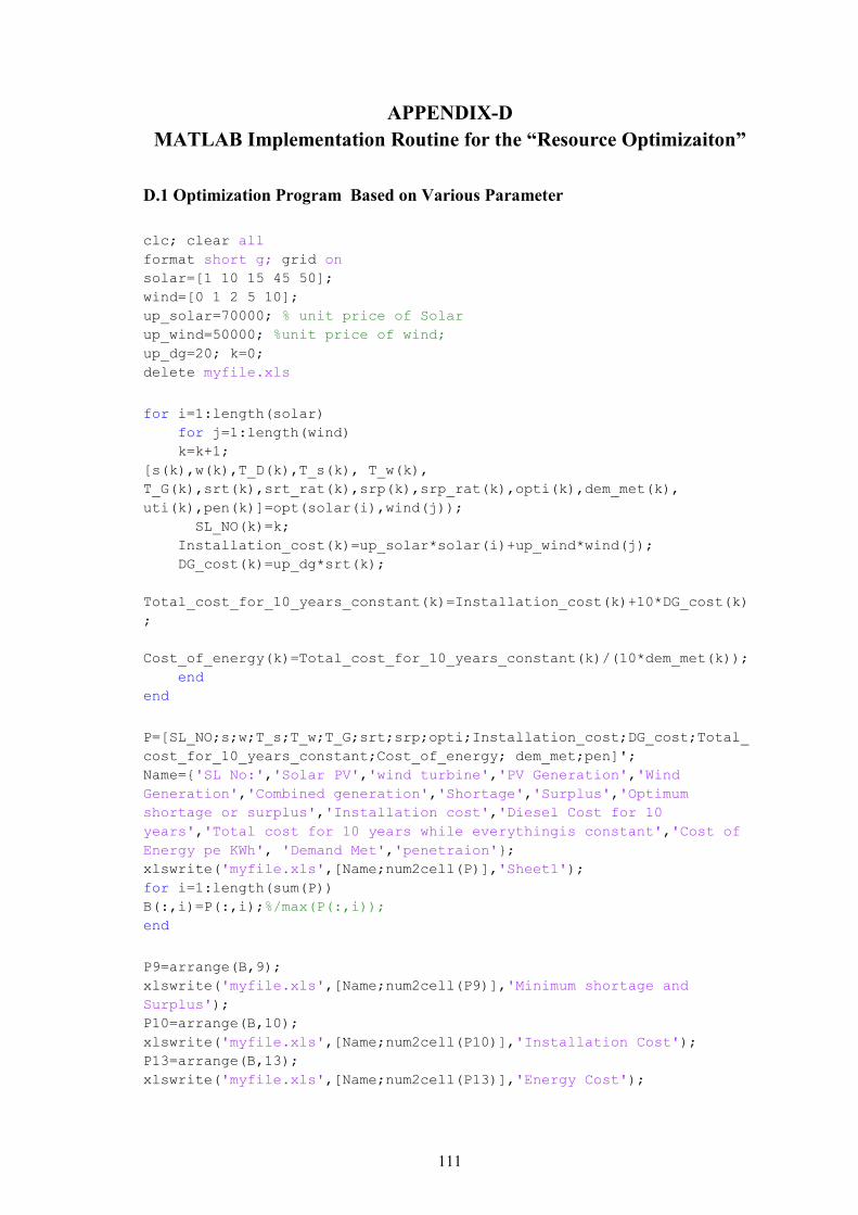
111

APPENDIX-D MATLAB Implementation Routine for the “Resource Optimizaiton”

D.1 Optimization Program Based on Various Parameter clc; clear all

format short g; grid on

solar=[1 10 15 45 50];

wind=[0 1 2 5 10];

up_solar=70000; % unit price of Solar

up_wind=50000; %unit price of wind;

up_dg=20; k=0;

delete myfile.xls

for i=1:length(solar)

for j=1:length(wind)

k=k+1;

[s(k),w(k),T_D(k),T_s(k), T_w(k),

T_G(k),srt(k),srt_rat(k),srp(k),srp_rat(k),opti(k),dem_met(k),

uti(k),pen(k)]=opt(solar(i),wind(j));

SL_NO(k)=k;

Installation_cost(k)=up_solar*solar(i)+up_wind*wind(j);

DG_cost(k)=up_dg*srt(k);

Total_cost_for_10_years_constant(k)=Installation_cost(k)+10*DG_cost(k)

;

Cost_of_energy(k)=Total_cost_for_10_years_constant(k)/(10*dem_met(k));

end

end

P=[SL_NO;s;w;T_s;T_w;T_G;srt;srp;opti;Installation_cost;DG_cost;Total_

cost_for_10_years_constant;Cost_of_energy; dem_met;pen]';

Name='SL No:','Solar PV','wind turbine','PV Generation','Wind

Generation','Combined generation','Shortage','Surplus','Optimum

shortage or surplus','Installation cost','Diesel Cost for 10

years','Total cost for 10 years while everythingis constant','Cost of

Energy pe KWh', 'Demand Met','penetraion';

xlswrite('myfile.xls',[Name;num2cell(P)],'Sheet1');

for i=1:length(sum(P))

B(:,i)=P(:,i);%/max(P(:,i));

end

P9=arrange(B,9);

xlswrite('myfile.xls',[Name;num2cell(P9)],'Minimum shortage and

Surplus');

P10=arrange(B,10);

xlswrite('myfile.xls',[Name;num2cell(P10)],'Installation Cost');

P13=arrange(B,13);

xlswrite('myfile.xls',[Name;num2cell(P13)],'Energy Cost');

112

D.2 The „opt‟ Function used in Program D.1 function [i,j,total_demand,gen_sol, gen_wind, total_generation,

shortage,shortage_ratio,surplus,surplus_ratio,optimum,demand_met,utili

zation,penetration]=opt(a,b)

Demand=[ 4400 4400 5350 5250 5500 5800 6400 6000 5850 5400 4450 4150];

u_a=[113 107 125 122 112 96 86 91 91 107 106 111];%unit production of

a

u_b=[200 207 225 220 192 196 186 291 191 207 210 210];%unit production

of b

format short g;

Demand=(.92+0.1*rand())*[ 4400 4400 5350 5250 5500 5800 6400 6000 5850

5400 4450 4150];

u_a=(.92+0.1*rand())*[113 107 125 122 112 96 86 91 91 107 106

111];%unit production of a

u_b=(.92+0.1*rand())*[200 207 225 220 192 196 186 191 191 207 210

210];%unit production of b

%a=5 ; %b=30

t_a=a*u_a; %Total production of a

t_b=b*u_b; %Total production of b

t_g=t_a+t_b; %%total production of a and b

diff=t_g-Demand;

shortage=(abs(diff)-diff)/2;

surplus=(abs(diff)+diff)/2;

util=Demand-shortage;

i=a;

j=b;

total_demand=sum(Demand);

gen_sol=sum(t_a);

gen_wind=sum(t_b);

total_generation=sum(t_g);

shortage=sum(shortage);

shortage_ratio=shortage/sum(t_g);

surplus=sum(surplus);

surplus_ratio=surplus/sum(t_g);

optimum=surplus-shortage;

demand_met=sum(util);

utilization=sum(util)/total_generation;

penetration=sum(util)/total_demand;

end

113

D.3 The “arrange” Function Used in Program D.1

function [C]=arrange(A,i)

format short g;

b=A(:,i);

c=sort(b);

k=0;

temp=0;

i=1;

while (i<=length(b))

temp=find(c(i)==b);

i=i+length(temp) ;

k=[k;temp];

end

k=k(2:end,:) ;

for i=1:length(k)

C(i,:)=A(k(i),:);

end

end

D.4 A similar program of D.1 but this program deals with more parameter than D.1 %arrange function has been added

clc

clear all

format short g

grid on

%solar=5;%1:50;

solar=[1 10 15];

%wind=25%;1:40

wind=[0 5 10];

biogas= [3 8 12];

up_solar=70000; % unit price of Solar

up_wind=50000; %unit price of wind;

up_bio=20000;

up_dg=20;

k=0;

%delete myfile.xls

for i=1:length(solar)

for j=1:length(wind)

for p=1:length(biogas)

k=k+1;

[s(k),w(k),b(k),T_D(k),T_s(k), T_w(k),T_b(k),

T_G(k),srt(k),srt_rat(k),srp(k),srp_rat(k),opti(k),dem_met(k),

uti(k),pen(k)]=optimization_3_parameter(solar(i),wind(j), biogas(p));

SL_NO(k)=k;

Installation_cost(k)=up_solar*solar(i)+up_wind*wind(j)+up_bio*biogas(p

);

114

DG_cost(k)=up_dg*srt(k);

Total_cost_for_10_years_constant(k)=Installation_cost(k)+10*DG_cost(k)

;

Cost_of_energy(k)=Total_cost_for_10_years_constant(k)/(10*dem_met(k));

end

end

end

P=[SL_NO;s;w;b; T_s;T_w;T_b;T_G; srt;DG_cost;srp;dem_met;

pen;Installation_cost;Cost_of_energy

;Total_cost_for_10_years_constant]';

Name='SL No:','Solar PV','Wind Turbine', 'Biogas','PV

Generation','Wind Generation','Biogas Generation','Combined Total

Generation','Shortage met by Diesel Generator','Yearly Diesel

Cost','Surplus', 'Demand Met','penetraion','Installation cost','Cost

of Energy pe KWh','Total cost for 10 years'

xlswrite('myfile.xls',[Name;num2cell(P)],'Sheet1');

for i=1:length(sum(P))

B(:,i)=P(:,i);%/max(P(:,i));

end

P12=arrange(B,12);

xlswrite('myfile.xls',[Name;num2cell(P12)],'Demand Met');

P13=arrange(B,13);

xlswrite('myfile.xls',[Name;num2cell(P13)],'Penetration');

P14=arrange(B,14);

xlswrite('myfile.xls',[Name;num2cell(P14)],'Installation Cost');

P15=arrange(B,15);

xlswrite('myfile.xls',[Name;num2cell(P15)],'Energy Cost');

D.5 The function “optimization_3_parameter” used in D.4 function [i,j,k,total_demand,gen_solar, gen_wind,gen_biogas,

total_generation,

shortage,shortage_ratio,surplus,surplus_ratio,optimum,demand_met,utili

zation,penetration]=optimization_3_parameter(a,b,c)

Demand=[ 4400 4400 5350 5250 5500 5800 6400 6000 5850 5400 4450 4150];

%u_a=[113 107 125 122 112 96 86 91 91 107 106 111];%unit production of

a

G_G12=[101 99 122 124 118 102 92 94 91 101 95 97];

u_a=G_G12;

u_b=[200 207 225 220 192 196 186 291 191 207 210 210];%unit production

of b

u_c=[160 180 170 175 165 160 165 160 155 150 155 160];%unit production

of c

format short g;

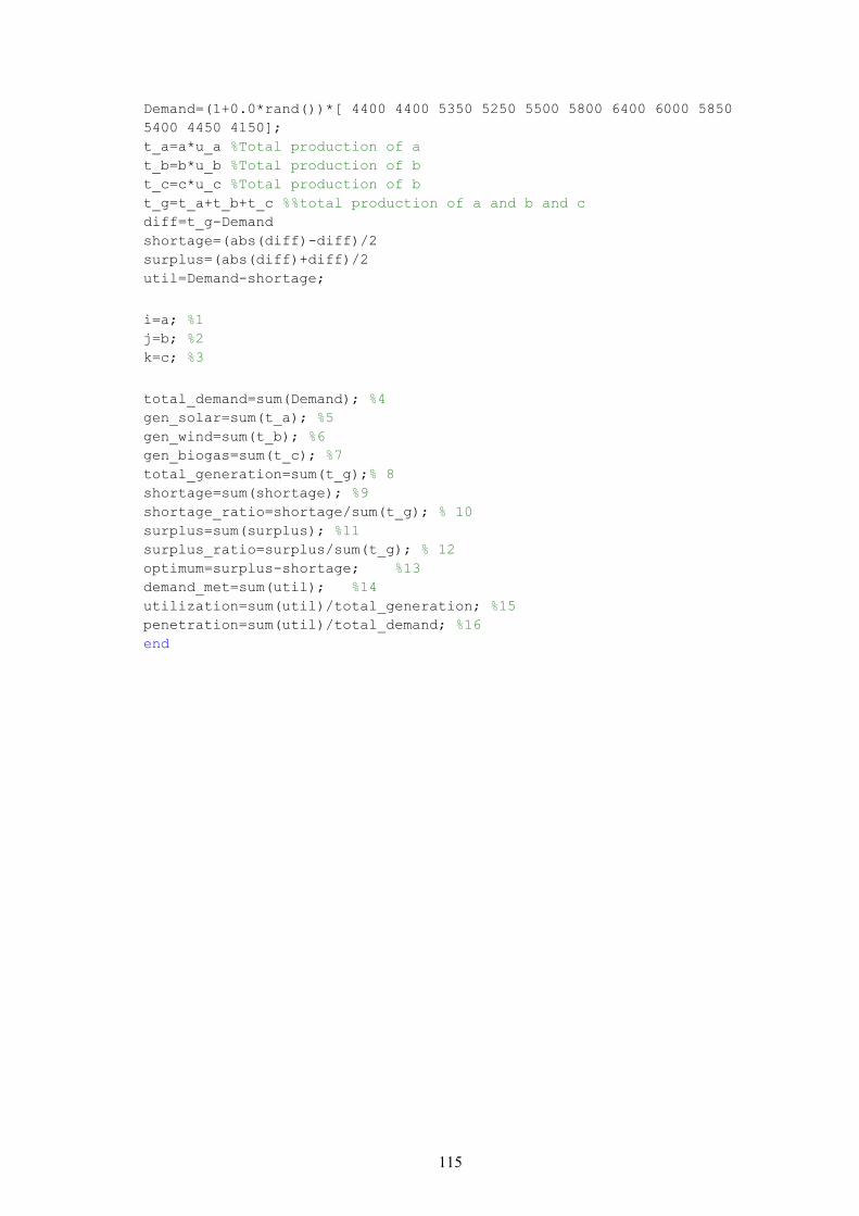
115

Demand=(1+0.0*rand())*[ 4400 4400 5350 5250 5500 5800 6400 6000 5850

5400 4450 4150];

t_a=a*u_a %Total production of a

t_b=b*u_b %Total production of b

t_c=c*u_c %Total production of b

t_g=t_a+t_b+t_c %%total production of a and b and c

diff=t_g-Demand

shortage=(abs(diff)-diff)/2

surplus=(abs(diff)+diff)/2

util=Demand-shortage;

i=a; %1

j=b; %2

k=c; %3

total_demand=sum(Demand); %4

gen_solar=sum(t_a); %5

gen_wind=sum(t_b); %6

gen_biogas=sum(t_c); %7

total_generation=sum(t_g);% 8

shortage=sum(shortage); %9

shortage_ratio=shortage/sum(t_g); % 10

surplus=sum(surplus); %11

surplus_ratio=surplus/sum(t_g); % 12

optimum=surplus-shortage; %13

demand_met=sum(util); %14

utilization=sum(util)/total_generation; %15

penetration=sum(util)/total_demand; %16

end

116

APPENDIX-E Results of Solar, Biogas, Wind Diesel Hybrid System Analysis

The output

SL No:

Solar PV

Wind Turbine

Biogas

PV Generation

Wind Generation

Biogas Generation

Combined Total Generation

Shortage met by Diesel Generator

Yearly Diesel Cost Surplus

Demand Met Penetration Installation cost

Cost of Energy pe KWh

Total cost for 10 years

1 1 0 3 1236 0 5865 7101 55849 1116980 0 7101 0.112804 130000 159.1297 11299800

2 1 0 8 1236 0 15640 16876 46074 921480 0 16876 0.268086 230000 55.96587 9444800

3 1 0 12 1236 0 23460 24696 38254 765080 0 24696 0.392311 310000 32.23518 7960800

4 1 5 3 1236 12675 5865 19776 43174 863480 0 19776 0.314154 380000 45.58455 9014800

5 1 5 8 1236 12675 15640 29551 33399 667980 0 29551 0.469436 480000 24.22862 7159800

6 1 5 12 1236 12675 23460 37371 25579 511580 0 37371 0.593662 560000 15.18771 5675800

7 1 10 3 1236 25350 5865 32451 30499 609980 0 32451 0.515504 630000 20.73834 6729800

8 1 10 8 1236 25350 15640 42226 20724 414480 0 42226 0.670786 730000 11.54455 4874800

9 1 10 12 1236 25350 23460 50046 12904 258080 0 50046 0.795012 810000 6.775367 3390800

10 10 0 3 12360 0 5865 18225 44725 894500 0 18225 0.289515 760000 53.25103 9705000

11 10 0 8 12360 0 15640 28000 34950 699000 0 28000 0.444797 860000 28.03571 7850000

12 10 0 12 12360 0 23460 35820 27130 542600 0 35820 0.569023 940000 17.77219 6366000

13 10 5 3 12360 12675 5865 30900 32050 641000 0 30900 0.490866 1010000 24.01294 7420000

14 10 5 8 12360 12675 15640 40675 22275 445500 0 40675 0.646148 1110000 13.68162 5565000

15 10 5 12 12360 12675 23460 48495 14455 289100 0 48495 0.770373 1190000 8.415301 4081000

16 10 10 3 12360 25350 5865 43575 19375 387500 0 43575 0.692216 1260000 11.78428 5135000

17 10 10 8 12360 25350 15640 53350 9900 198000 300 53050 0.842732 1360000 6.295947 3340000

18 10 10 12 12360 25350 23460 61170 4880 97600 3100 58070 0.922478 1440000 4.160496 2416000

19 15 0 3 18540 0 5865 24405 38545 770900 0 24405 0.387689 1110000 36.13604 8819000

20 15 0 8 18540 0 15640 34180 28770 575400 0 34180 0.542971 1210000 20.37449 6964000

21 15 0 12 18540 0 23460 42000 20950 419000 0 42000 0.667196 1290000 13.04762 5480000

22 15 5 3 18540 12675 5865 37080 25870 517400 0 37080 0.589039 1360000 17.62136 6534000

27 15 10 12 18540 25350 23460 67350 2300 46000 6700 60650 0.963463 1790000 3.70981 2250000

117

Optimization according to Demand Met

SL No:

Solar PV

Wind Turbine

Biogas

PV Generati

on

Wind Generation

Biogas Generation

Combined Total Generati

on

Shortage met by Diesel

Generator

Yearly Diesel Cost

Surplus Demand Met

Penetration Installation cost



1 1 0 3 1236 0 5865 7101 55849 1116980 0 7101 0.112804 130000 159.1297 11299800

2 1 0 8 1236 0 15640 16876 46074 921480 0 16876 0.268086 230000 55.96587 9444800

10 10 0 3 12360 0 5865 18225 44725 894500 0 18225 0.289515 760000 53.25103 9705000

4 1 5 3 1236 12675 5865 19776 43174 863480 0 19776 0.314154 380000 45.58455 9014800

19 15 0 3 18540 0 5865 24405 38545 770900 0 24405 0.387689 1110000 36.13604 8819000

3 1 0 12 1236 0 23460 24696 38254 765080 0 24696 0.392311 310000 32.23518 7960800

11 10 0 8 12360 0 15640 28000 34950 699000 0 28000 0.444797 860000 28.03571 7850000

5 1 5 8 1236 12675 15640 29551 33399 667980 0 29551 0.469436 480000 24.22862 7159800

13 10 5 3 12360 12675 5865 30900 32050 641000 0 30900 0.490866 1010000 24.01294 7420000

7 1 10 3 1236 25350 5865 32451 30499 609980 0 32451 0.515504 630000 20.73834 6729800

20 15 0 8 18540 0 15640 34180 28770 575400 0 34180 0.542971 1210000 20.37449 6964000

12 10 0 12 12360 0 23460 35820 27130 542600 0 35820 0.569023 940000 17.77219 6366000

22 15 5 3 18540 12675 5865 37080 25870 517400 0 37080 0.589039 1360000 17.62136 6534000

6 1 5 12 1236 12675 23460 37371 25579 511580 0 37371 0.593662 560000 15.18771 5675800

14 10 5 8 12360 12675 15640 40675 22275 445500 0 40675 0.646148 1110000 13.68162 5565000

21 15 0 12 18540 0 23460 42000 20950 419000 0 42000 0.667196 1290000 13.04762 5480000

8 1 10 8 1236 25350 15640 42226 20724 414480 0 42226 0.670786 730000 11.54455 4874800

16 10 10 3 12360 25350 5865 43575 19375 387500 0 43575 0.692216 1260000 11.78428 5135000

23 15 5 8 18540 12675 15640 46855 16095 321900 0 46855 0.744321 1460000 9.986127 4679000

15 10 5 12 12360 12675 23460 48495 14455 289100 0 48495 0.770373 1190000 8.415301 4081000

25 15 10 3 18540 25350 5865 49755 13195 263900 0 49755 0.790389 1610000 8.539845 4249000

9 1 10 12 1236 25350 23460 50046 12904 258080 0 50046 0.795012 810000 6.775367 3390800

17 10 10 8 12360 25350 15640 53350 9900 198000 300 53050 0.842732 1360000 6.295947 3340000

24 15 5 12 18540 12675 23460 54675 8865 177300 590 54085 0.859174 1540000 6.125543 3313000

118

Optimization according to Penetration

SL No:

Solar PV

Wind Turbine

Biogas

PV Generation

Wind Generation

Biogas Generation




Demand Met Penetration Installation cost



1 1 0 3 1236 0 5865 7101 55849 1116980 0 7101 0.112804 130000 159.1297 11299800

2 1 0 8 1236 0 15640 16876 46074 921480 0 16876 0.268086 230000 55.96587 9444800

10 10 0 3 12360 0 5865 18225 44725 894500 0 18225 0.289515 760000 53.25103 9705000

4 1 5 3 1236 12675 5865 19776 43174 863480 0 19776 0.314154 380000 45.58455 9014800

19 15 0 3 18540 0 5865 24405 38545 770900 0 24405 0.387689 1110000 36.13604 8819000

3 1 0 12 1236 0 23460 24696 38254 765080 0 24696 0.392311 310000 32.23518 7960800

11 10 0 8 12360 0 15640 28000 34950 699000 0 28000 0.444797 860000 28.03571 7850000

5 1 5 8 1236 12675 15640 29551 33399 667980 0 29551 0.469436 480000 24.22862 7159800

13 10 5 3 12360 12675 5865 30900 32050 641000 0 30900 0.490866 1010000 24.01294 7420000

7 1 10 3 1236 25350 5865 32451 30499 609980 0 32451 0.515504 630000 20.73834 6729800

20 15 0 8 18540 0 15640 34180 28770 575400 0 34180 0.542971 1210000 20.37449 6964000

12 10 0 12 12360 0 23460 35820 27130 542600 0 35820 0.569023 940000 17.77219 6366000

22 15 5 3 18540 12675 5865 37080 25870 517400 0 37080 0.589039 1360000 17.62136 6534000

6 1 5 12 1236 12675 23460 37371 25579 511580 0 37371 0.593662 560000 15.18771 5675800

14 10 5 8 12360 12675 15640 40675 22275 445500 0 40675 0.646148 1110000 13.68162 5565000

21 15 0 12 18540 0 23460 42000 20950 419000 0 42000 0.667196 1290000 13.04762 5480000

8 1 10 8 1236 25350 15640 42226 20724 414480 0 42226 0.670786 730000 11.54455 4874800

16 10 10 3 12360 25350 5865 43575 19375 387500 0 43575 0.692216 1260000 11.78428 5135000

23 15 5 8 18540 12675 15640 46855 16095 321900 0 46855 0.744321 1460000 9.986127 4679000

15 10 5 12 12360 12675 23460 48495 14455 289100 0 48495 0.770373 1190000 8.415301 4081000

25 15 10 3 18540 25350 5865 49755 13195 263900 0 49755 0.790389 1610000 8.539845 4249000

9 1 10 12 1236 25350 23460 50046 12904 258080 0 50046 0.795012 810000 6.775367 3390800

17 10 10 8 12360 25350 15640 53350 9900 198000 300 53050 0.842732 1360000 6.295947 3340000

24 15 5 12 18540 12675 23460 54675 8865 177300 590 54085 0.859174 1540000 6.125543 3313000

119

Optimization according to Installation Cost

SL No:

Solar PV

Wind Turbine

Biogas

PV Generation

Wind Generation

Biogas Generation




Demand Met Penetration

Installation cost



1 1 0 3 1236 0 5865 7101 55849 1116980 0 7101 0.112804 130000 159.1297 11299800

2 1 0 8 1236 0 15640 16876 46074 921480 0 16876 0.268086 230000 55.96587 9444800

3 1 0 12 1236 0 23460 24696 38254 765080 0 24696 0.392311 310000 32.23518 7960800

4 1 5 3 1236 12675 5865 19776 43174 863480 0 19776 0.314154 380000 45.58455 9014800

5 1 5 8 1236 12675 15640 29551 33399 667980 0 29551 0.469436 480000 24.22862 7159800

6 1 5 12 1236 12675 23460 37371 25579 511580 0 37371 0.593662 560000 15.18771 5675800

7 1 10 3 1236 25350 5865 32451 30499 609980 0 32451 0.515504 630000 20.73834 6729800

8 1 10 8 1236 25350 15640 42226 20724 414480 0 42226 0.670786 730000 11.54455 4874800

10 10 0 3 12360 0 5865 18225 44725 894500 0 18225 0.289515 760000 53.25103 9705000

9 1 10 12 1236 25350 23460 50046 12904 258080 0 50046 0.795012 810000 6.775367 3390800

11 10 0 8 12360 0 15640 28000 34950 699000 0 28000 0.444797 860000 28.03571 7850000

12 10 0 12 12360 0 23460 35820 27130 542600 0 35820 0.569023 940000 17.77219 6366000

13 10 5 3 12360 12675 5865 30900 32050 641000 0 30900 0.490866 1010000 24.01294 7420000

14 10 5 8 12360 12675 15640 40675 22275 445500 0 40675 0.646148 1110000 13.68162 5565000

19 15 0 3 18540 0 5865 24405 38545 770900 0 24405 0.387689 1110000 36.13604 8819000

15 10 5 12 12360 12675 23460 48495 14455 289100 0 48495 0.770373 1190000 8.415301 4081000

20 15 0 8 18540 0 15640 34180 28770 575400 0 34180 0.542971 1210000 20.37449 6964000

16 10 10 3 12360 25350 5865 43575 19375 387500 0 43575 0.692216 1260000 11.78428 5135000

21 15 0 12 18540 0 23460 42000 20950 419000 0 42000 0.667196 1290000 13.04762 5480000

17 10 10 8 12360 25350 15640 53350 9900 198000 300 53050 0.842732 1360000 6.295947 3340000

22 15 5 3 18540 12675 5865 37080 25870 517400 0 37080 0.589039 1360000 17.62136 6534000

18 10 10 12 12360 25350 23460 61170 4880 97600 3100 58070 0.922478 1440000 4.160496 2416000

23 15 5 8 18540 12675 15640 46855 16095 321900 0 46855 0.744321 1460000 9.986127 4679000

24 15 5 12 18540 12675 23460 54675 8865 177300 590 54085 0.859174 1540000 6.125543 3313000

120

Optimization according to Cost of Energy

SL No:

Solar PV

Wind Turbine

Biogas

PV Generation

Wind Generation

Biogas Generation




Demand Met Penetration

Installation cost



27 15 10 12 18540 25350 23460 67350 2300 46000 6700 60650 0.963463 1790000 3.70981 2250000

18 10 10 12 12360 25350 23460 61170 4880 97600 3100 58070 0.922478 1440000 4.160496 2416000

26 15 10 8 18540 25350 15640 59530 5710 114200 2290 57240 0.909293 1710000 4.98253 2852000

24 15 5 12 18540 12675 23460 54675 8865 177300 590 54085 0.859174 1540000 6.125543 3313000

17 10 10 8 12360 25350 15640 53350 9900 198000 300 53050 0.842732 1360000 6.295947 3340000

9 1 10 12 1236 25350 23460 50046 12904 258080 0 50046 0.795012 810000 6.775367 3390800

15 10 5 12 12360 12675 23460 48495 14455 289100 0 48495 0.770373 1190000 8.415301 4081000

25 15 10 3 18540 25350 5865 49755 13195 263900 0 49755 0.790389 1610000 8.539845 4249000

23 15 5 8 18540 12675 15640 46855 16095 321900 0 46855 0.744321 1460000 9.986127 4679000

8 1 10 8 1236 25350 15640 42226 20724 414480 0 42226 0.670786 730000 11.54455 4874800

16 10 10 3 12360 25350 5865 43575 19375 387500 0 43575 0.692216 1260000 11.78428 5135000

21 15 0 12 18540 0 23460 42000 20950 419000 0 42000 0.667196 1290000 13.04762 5480000

14 10 5 8 12360 12675 15640 40675 22275 445500 0 40675 0.646148 1110000 13.68162 5565000

6 1 5 12 1236 12675 23460 37371 25579 511580 0 37371 0.593662 560000 15.18771 5675800

22 15 5 3 18540 12675 5865 37080 25870 517400 0 37080 0.589039 1360000 17.62136 6534000

12 10 0 12 12360 0 23460 35820 27130 542600 0 35820 0.569023 940000 17.77219 6366000

20 15 0 8 18540 0 15640 34180 28770 575400 0 34180 0.542971 1210000 20.37449 6964000

7 1 10 3 1236 25350 5865 32451 30499 609980 0 32451 0.515504 630000 20.73834 6729800

13 10 5 3 12360 12675 5865 30900 32050 641000 0 30900 0.490866 1010000 24.01294 7420000

5 1 5 8 1236 12675 15640 29551 33399 667980 0 29551 0.469436 480000 24.22862 7159800

11 10 0 8 12360 0 15640 28000 34950 699000 0 28000 0.444797 860000 28.03571 7850000

3 1 0 12 1236 0 23460 24696 38254 765080 0 24696 0.392311 310000 32.23518 7960800

19 15 0 3 18540 0 5865 24405 38545 770900 0 24405 0.387689 1110000 36.13604 8819000

4 1 5 3 1236 12675 5865 19776 43174 863480 0 19776 0.314154 380000 45.58455 9014800

121

APPENDIX-F

Determination of Maximum Voltage between Two Isolated Microgrids when Interconnected”

F.1 Program for “voltage_drop.m”

clear all

len=100:50:1000

format long

r=230^2/(10000/0.8);

Zload= r*(0.8+0.6i)

for k=1:length(len)

R=0.0017719*len(k);

L=len(k)*1e-7*(1+4*log(50/1)) %% 1000 is for 1KM

C=len(k)*pi*8.854e-12/(log(50/1))%% 1000 is for 1KM

XL=i*2*pi*50*L

XC=1/(i*2*pi*50*C)

Ztemp=1/((1/XC)+(1/Zload))

Zline=R+XL

Ztotal=Zline+Ztemp

Current=230/Ztotal

Voltage(k)=abs(Ztemp*Current)

drop(k)=abs(Zline*Current)

end

plot(len,drop,'y', 'LineWidth',3)

hold on

plot(len,Voltage,'r', 'LineWidth',3)

grid on

legend('Voltage Drop in Interconnection line','VOltage at Node 2')

xlabel('Distance of Node 2 from Node 1', 'FontSize',13);

ylabel('Voltage', 'FontSize',13);

title('Distance Vs Voltage drop and Voltage at Node 2')

122

APPENDIX-G Determination of Maximum Voltage between Two Isolated Microgrids

When Interconnected”

G.1 Policy01.m

clear all

clc

clf

% In this program, it is assumed that entity 1 will install 10KWp of

% solar PV and 45 unit of entity 2 type CPU (each having 2KWp) will

% provide 90KWp of solar PV. Thus a total of 100KWp Solar PV. The battery

% backup for the complete system will be provided by the entity 1

Buy_price= 10;% price of buy per unit of energy(per KWh) from entity 2,

it is changed manually for each iteration

Sale_price=35;% price of sale per unit of energy(per KWh) to entity 2, it

is changed manually for each iteration as 20, 25, 30 and 35

for i=Buy_price:Sale_price-1

Usable_energy=1300; % KWh per year

Panel_2=2; % in KWp, 2KWp is assumed as the unit installtion size of each

CPU

Panel_Price_unit=60000;% per KWp

Panel_price_total=Panel_2*Panel_Price_unit;

CPU_cost= 20000; % per KWp and others

CPU_cost_total= Panel_2*CPU_cost;

Total_investment=Panel_price_total+CPU_cost_total;

Running_cost=0.02*Total_investment; % 2% of initial investment

Energy=Usable_energy*Panel_2;

Revenue=Energy*i;

Net_Profit= Revenue-Running_cost;

return_2=Total_investment/Net_Profit; % payback period for entity 2

Panel_1=10; %10 KWp is assumed to be the size of authority 1 power source

Panel=Panel_1*1000*60; %60,000 per KWp

Battery = 4800000; % For 10KWp Authority 1 + 90 KWp from authority 2

123

Distribution_System= 5*80000; % 5km and 80,000 for each km

%Pole 55

Diesel_generator=3*200000; %10KW Generator, no 3

Others=10*10000; % 10,000 per KWp

connection_charge= 200*5000; % 5000 BDT per connection

Initial_cost= Panel+ Battery+ Distribution_System+ Diesel_generator+

Others - connection_charge; %65,00,000

Energy_1= Usable_energy*Panel_1; % 10KWp comes from entity 1

Energy_2= Usable_energy*Panel_2*45; % 45 number of CPU, each have 2KWp

solar panel = 90KWp from entity 2

Energy_panel= Energy_1+Energy_2;

Energy_loss=Energy_panel*0.04; % loss due to battery charging and

discharging

Energy_panel_use=Energy_panel-Energy_loss;

Energy_DG= 0.3*Energy_panel_use/0.7; % Assume 30% of Total energy comes

from DG

Energy_sale=Energy_panel_use+Energy_DG;

Energy_sale_price=Energy_sale*Sale_price;

Energy_2_cost=Energy_2*i; % total cost to buy energy from entity 2

Energy_DG_cost=Energy_DG*15; % Assumed to be same as Sandwip DG cost

Yearly_Running_Cost= 400000; % Sandwip employee + other maintenance

cost

Yearly_cost=Energy_2_cost+ Energy_DG_cost + Yearly_Running_Cost; %

Yearly_profit=Energy_sale_price-Yearly_cost;

return_1=Initial_cost/Yearly_profit;

R_1(i)=return_1;

R_2(i)=return_2;

diff(i)=return_1-return_2;

end

plot(R_1,'r', 'LineWidth', 3)

hold on

grid on

plot(R_2,'LineWidth', 3)

xlim([22, 28]) % this limit is changed in each iteration for better view

of produced image

legend('Entity 1','Entity 2')

xlabel('Buying Price of energy from entity 2 in BDT', 'FontSize',12);

ylabel('Simple Payback period in Years', 'FontSize',12);

124

G.2 Policy02.m clear all

clc

clf

% In this program, it is assumed that entity 1 will install 10KWp of

% solar PV and 45 unit of entity 2 type CPU (each having 2KWp) will

% provide 90KWp of solar PV. Thus a total of 100KWp Solar PV. The battery

% backup for the complete system will be provided by the entity 1

Buy_price= 25;% price of buy per unit of energy(per KWh) from entity 2,

it is changed manually for each iteration as 10, 15, 20, 25

Sale_price=40;% price of sale per unit of energy(per KWh) to entity 2, it

is changed manually for each iteration

for i=Buy_price+1:Sale_price

Usable_energy=1300; % KWh per year

Panel_2=2; % in KWp, 2KWp is assumed as the unit installtion size

of each CPU

Panel_Price_unit=60000;% per KWp

Panel_price_total=Panel_2*Panel_Price_unit;

CPU_cost= 20000; % per KWp and others

CPU_cost_total= Panel_2*CPU_cost;

Total_investment=Panel_price_total+CPU_cost_total;

Running_cost=0.02*Total_investment; % 2% of initial investment

Energy=Usable_energy*Panel_2;

Revenue=Energy*Buy_price;

Net_Profit= Revenue-Running_cost;

return_2=Total_investment/Net_Profit; % payback period for entity 2

Panel_1=10; %10 KWp is assumed to be the size of authority 1

power source

Panel=Panel_1*1000*60; %60,000 per KWp

Battery = 4800000; % For 10KWp Authority 1 + 90 KWp from

authority 2

Distribution_System= 5*80000; % 5km and 80,000 for each km

%Pole 55

Diesel_generator=3*200000; %10KW Generator, no 3

Others=10*10000; % 10,000 per KWp

connection_charge= 200*5000; % 5000 BDT per connection

Initial_cost= Panel+ Battery+ Distribution_System+

Diesel_generator+ Others - connection_charge; %65,00,000

Energy_1= Usable_energy*Panel_1; % 10KWp comes from entity 1

125

Energy_2= Usable_energy*Panel_2*45; % 45 number of CPU, each have

2KWp solar panel = 90KWp from entity 2

Energy_panel= Energy_1+Energy_2;

Energy_loss=Energy_panel*0.04; % loss due to battery charging and

discharging

Energy_panel_use=Energy_panel-Energy_loss;

Energy_DG= 0.3*Energy_panel_use/0.7; % Assume 30% of Total energy

comes from DG

Energy_sale=Energy_panel_use+Energy_DG;

Energy_2_cost=Energy_2*Buy_price; % total cost to buy energy from

entity 2

Energy_DG_cost=Energy_DG*15; % Assumed to be same as Sandwip DG

cost

Yearly_Running_Cost= 400000; % Sandwip employee + other

maintenance cost

Yearly_cost=Energy_2_cost+ Energy_DG_cost + Yearly_Running_Cost;

%

Energy_sale_price=Energy_sale*i;

Yearly_profit=Energy_sale_price-Yearly_cost;

return_1=Initial_cost/Yearly_profit;

R_1(i)=return_1;

R_2(i)=return_2;

diff(i)=return_1-return_2;

end

plot(R_1,'r', 'LineWidth', 3)

hold on

grid on

plot(R_2,'LineWidth', 3)

xlim([33, 37]) % this limit is changed in each iteration for better view

of produced image

legend('Entity 1','Entity 2')

xlabel('Price of sales of energy by entity 1 in BDT', 'FontSize',12);

ylabel('Simple Payback period in Years', 'FontSize',12);

126

APPENDIX-H Projection about the Installed Capacity

H.1 time_projection.m clc

clear all

n=1

m=20

acs=2; %avgerage CPU Size in KW

year=n:m;

%%% idcol is the number of instllation

idcol=[772 15745 36380 63959 101110 170672 285773 455689 780756 1254923

1700000 2700000 4288235.294 6810726.644 10817036.43 17179999.04

27285880.83 43336398.97 68828398.36 109315691.5 173619039.5 275747886.2

437952525.2 695571657.6 1104731456];

cip=acs*idcol(:,n:m);

pro_200= 2*cip/1000;

pro_150= 1.5*cip/1000;

pro_100= cip/1000;

pro_90= 0.9*cip/1000;

pro_80= 0.8*cip/1000;

pro_70= 0.7*cip/1000;

pro_50= 0.5*cip/1000;

pro= round([pro_200(m) pro_150(m) pro_100(m) pro_80(m) pro_50(m)])

h=figure

plot(year,pro_200,'r', 'LineWidth',3)

hold on

grid on

plot(year,pro_150,'y', 'LineWidth',3)

plot(year,pro_100,'c', 'LineWidth',3)

plot(year,pro_90,'m', 'LineWidth',3)

plot(year,pro_80,'b', 'LineWidth',3)

plot(year,pro_70,'g', 'LineWidth',3)

plot(year,pro_50,'k', 'LineWidth',3)

legend('200% rate of SHS','150% rate of SHS','100% rate of SHS','90% rate

of SHS','80% rate of SHS','70% rate of SHS','50% rate of

SHS','Location','Best')

xlabel('Year after program start', 'FontSize',13);

ylabel('Forcasted installed capacity MWp', 'FontSize',13);

title('10-20 years projection')

%saveas(h,'1-5 years projection','jpg')

analysis of an electrical microgrid in a remote area based

Documents