analysis of cardinal and ordinal assumptions in conjoint...

Analysis of Cardinal and Ordinal Assumptions in Conjoint Analysis R. Wes Harrison, Jeffrey Gillespie, and Deacue Fields Of twenty-three agricultural economics conjoint analyses conducted between 1990 and 2001,

seventeen used interval-rating scales, with estimation procedures varying widely. This study tests cardinality assumptions in conjoint analysis when interval-rating scales are used, and tests whether the ordered probit or two-limit tobit model is the most valid. Results indicate that cardinality assumptions are invalid, but estimates of the underlying utility scale for the two models do not differ. Thus, while the ordered probit model is theoretically more appealing, the two-limit tobit model may be more useful in practice, especially in cases with limited degrees of freedom, such as with individual-level conjoint models.

Key Words: ordered probit, two-limit probit, conjoint analysis, cardinality Numerous applications of conjoint analysis (CA) have emerged in the agricultural economics litera-ture in recent years. Most of these studies have analyzed consumer preferences for new food products or resource usage and willingness to pay for recreational services. Studies evaluating new food products include Gineo (1990), Prentice and Benell (1992), Halbrendt, Wirth, and Vaughn (1991), Halbrendt, Bacon, and Pesek (1992), Yoo and Ohta (1995), Hobbs (1996), Sylvia and Larkin (1995), Sy et al. (1997), Harrison, Ozayan, and Meyers (1998), Gillespie et al. (1998), and Holland and Wessells (1998). New product ac-ceptance studies typically assume that a respon-dent’s total utility for a hypothetical product is a function of various product attributes. CA is used to estimate “part-worth” utilities, which measure the partial effect of a particular attribute level on the respondent’s total utility for hypothetical products. Part-worth estimates are typically used to simulate utility values for products not evalu-ated by respondents; thus, optimal hypothetical products can be determined. A second category of CA studies has sought to estimate respondents’ willingness to pay for a bundle of attributes associated with a recreational

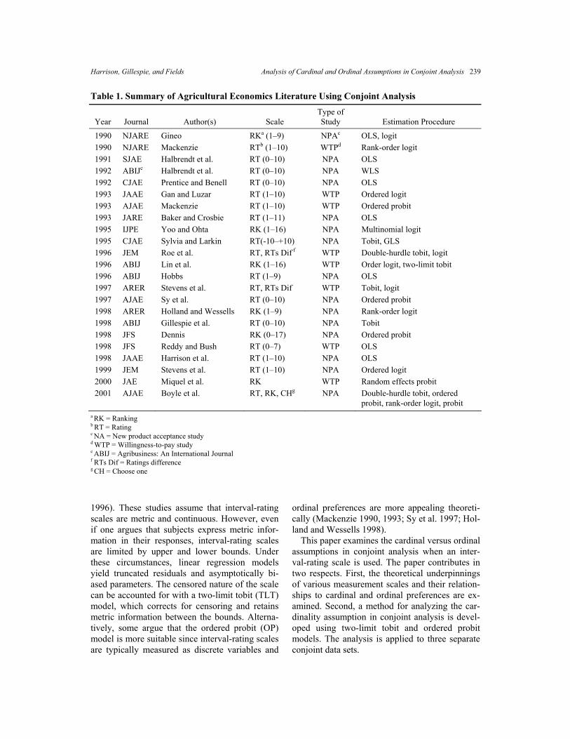
site or activity. Examples include Mackenzie (1990, 1993), Gan and Luzar (1993), Lin, Pay-son, and Wertz (1996), Roe, Boyle, and Teisl (1996), Stevens, Barrett, and Willis (1997), Mi-quel, Ryan, and McIntosh (2000), and Boyle et al. (2001). As with the new product acceptance stud-ies, this approach requires respondents to rate or rank attribute bundles as price and other attribute levels are varied (Mackenzie 1990). Willingness to pay is calculated directly from the marginal rates of substitution between price and non-price attributes estimated from conjoint data. Two commonly used methods for coding re-spondent preferences are rank-order and interval-rating scales. The rank-order method requires subjects to unambiguously rank all hypothetical product choices. In these cases, the dependent variable is ordinal, and ordered regression models such as ordered probit or logit are most suitable for conjoint estimation. The interval-rating method allows subjects to express order, indiffer-ence, and intensity across product choices, a fea-ture allowing both metric and nonmetric proper-ties of utility to be elicited. Model selection be-comes less clear if interval-rating scaling is used. As shown in Table 1, a wide range of models have been utilized when ratings have been used. Some studies have used linear regression to esti-mate part-worth parameters (Halbrendt, Wirth, and Vaughn 1991; Prentice and Benell 1992; Harrison, Ozayan, and Meyers 1998; Stevens, Barrett, and Willis 1997; Roe, Boyle, and Teisl

_________________________________________

R. Wes Harrison and Jeffrey Gillespie are Associate Professors in the Department of Agricultural Economics and Agribusiness at the Louisi-ana State University Agricultural Center in Baton Rouge, Louisiana. Deacue Fields is Assistant Professor in the Department of Agricultural Economics and Rural Sociology at Auburn University in Auburn, Alabama.

Agricultural and Resource Economics Review 34/2 (October 2005) 238–252 Copyright 2005 Northeastern Agricultural and Resource Economics Association

Harrison, Gillespie, and Fields Analysis of Cardinal and Ordinal Assumptions in Conjoint Analysis 239

Table 1. Summary of Agricultural Economics Literature Using Conjoint Analysis

Year Journal Author(s) Scale Type of Study Estimation Procedure

1990 NJARE Gineo RKa (1–9) NPAc OLS, logit 1990 NJARE Mackenzie RTb (1–10) WTPd Rank-order logit 1991 SJAE Halbrendt et al. RT (0–10) NPA OLS 1992 ABIJe Halbrendt et al. RT (0–10) NPA WLS 1992 CJAE Prentice and Benell RT (0–10) NPA OLS 1993 JAAE Gan and Luzar RT (1–10) WTP Ordered logit 1993 AJAE Mackenzie RT (1–10) WTP Ordered probit 1993 JARE Baker and Crosbie RT (1–11) NPA OLS 1995 IJPE Yoo and Ohta RK (1–16) NPA Multinomial logit 1995 CJAE Sylvia and Larkin RT(-10–+10) NPA Tobit, GLS 1996 JEM Roe et al. RT, RTs Dif f WTP Double-hurdle tobit, logit 1996 ABIJ Lin et al. RK (1–16) WTP Order logit, two-limit tobit 1996 ABIJ Hobbs RT (1–9) NPA OLS 1997 ARER Stevens et al. RT, RTs Dif WTP Tobit, logit 1997 AJAE Sy et al. RT (0–10) NPA Ordered probit 1998 ARER Holland and Wessells RK (1–9) NPA Rank-order logit 1998 ABIJ Gillespie et al. RT (0–10) NPA Tobit 1998 JFS Dennis RK (0–17) NPA Ordered probit 1998 JFS Reddy and Bush RT (0–7) WTP OLS 1998 JAAE Harrison et al. RT (1–10) NPA OLS 1999 JEM Stevens et al. RT (1–10) NPA Ordered logit 2000 JAE Miquel et al. RK WTP Random effects probit 2001 AJAE Boyle et al. RT, RK, CHg NPA Double-hurdle tobit, ordered

probit, rank-order logit, probit a RK = Ranking b RT = Rating c NA = New product acceptance study d WTP = Willingness-to-pay study e ABIJ = Agribusiness: An International Journal f RTs Dif = Ratings difference g CH = Choose one

1996). These studies assume that interval-rating scales are metric and continuous. However, even if one argues that subjects express metric infor-mation in their responses, interval-rating scales are limited by upper and lower bounds. Under these circumstances, linear regression models yield truncated residuals and asymptotically bi-ased parameters. The censored nature of the scale can be accounted for with a two-limit tobit (TLT) model, which corrects for censoring and retains metric information between the bounds. Alterna-tively, some argue that the ordered probit (OP) model is more suitable since interval-rating scales are typically measured as discrete variables and

ordinal preferences are more appealing theoreti-cally (Mackenzie 1990, 1993; Sy et al. 1997; Hol-land and Wessells 1998). This paper examines the cardinal versus ordinal assumptions in conjoint analysis when an inter-val-rating scale is used. The paper contributes in two respects. First, the theoretical underpinnings of various measurement scales and their relation-ships to cardinal and ordinal preferences are ex-amined. Second, a method for analyzing the car-dinality assumption in conjoint analysis is devel-oped using two-limit tobit and ordered probit models. The analysis is applied to three separate conjoint data sets.

October 2005 Agricultural and Resource Economics Review 240

_________________________________

Literature Review

The debate among economists as to whether car-dinal preferences can be assumed is not new. Van Praag (1991) discusses the history of the cardinal-ity-ordinality debate during the late nineteenth and early twentieth centuries. Cardinal utility was central in the development of demand theory and was largely unopposed throughout the nineteenth century (e.g., Jevons 1871, Menger 1981). The notion of a cardinal utility function was appealing because it yielded a robust theory of consumer demand and allowed for interpersonal compari-sons of utility. However, by the beginning of the twentieth century, some economists began to doubt whether cardinal utility actually existed, and whether it could be accurately measured. This led to Pareto’s (1909) assertion that it was not neces-sary to have an exact utility function to explain demand—that only indifference curves were needed. He showed that a broader class of ordi-nal, monotonically increasing functions is suffi-cient to derive all properties of demand. Pareto’s view was reinforced in the 1930s, as Robbins (1932) rejected the idea that cardinal utility was measurable at all. Other authors have given rigor-ous explanations of the theory of consumer de-mand in the absence of cardinal utility (e.g., Fisher 1918, Stigler 1950, Alchian 1953). Today, graduate-level microeconomics texts such as Var-ian (1947), Silberberg (1978), and Henderson and Quandt (1980) discuss the highly restrictive na-ture of cardinal preferences, and develop demand theory in the context of ordinal utility. In spite of these developments, economists remain interested in cardinal utility. Three areas of economics that assume some form of cardinal utility include (i) those estimating utility func-tions in an expected utility framework, in the spirit of von Neumann and Morgenstern (1947),1 (ii) studies using conjoint and other multi-attribute utility procedures to elicit strength of preferences, and (iii) studies on income equality and poverty in which interpersonal comparisons of utility are based.2 In each of these areas, it is

assumed that, while cardinal preferences are dif-ficult to measure with great precision, cardinal utility functions provide answers to “real world” questions.

1 Expected utility theory relaxes the assumption of pure ordinality. Additional axioms are introduced to allow for an expected utility function that is unique up to an affine transformation.

2 We should note that cardinal information does not solve all the problems associated with interpersonal comparison of utility. Even if an individual’s interval scale contains cardinal information, the mean-ing of the scale values may differ from one individual to another.

Several studies have analyzed the effects of treating an interval-rating scale as a cardinal measure of consumer preference (Mackenzie 1993; Roe, Boyle, and Teisl 1996; Stevens, Bar-rett, and Willis 1997). These studies compare parameter estimates and predictability of TLT with OP models, and have produced mixed re-sults. Mackenzie (1993) found evidence that rat-ing scales capture intensity (cardinality) in re-spondent preferences. The other two studies found empirical evidence suggesting the superior-ity of ordered probability models as frameworks for analysis and suggested that assuming ordinal preferences is theoretically more appealing. Boyle et al. (2001) examined cardinality by analyzing both rating and ranking scales for independent sub-samples of respondents. They found that TLT and OP models resulted in the same attributes being significant with the same signs. They con-cluded that assumptions regarding ordinal/car-dinal preferences were irrelevant for their sample. They did not, however, test the cardinality assump-tion or examine how well the models predicted preference ordering. More recently, Harrison, Stringer, and Priny-awiwatkul (2002) found little difference between the TLT and OP models with respect to part-worth estimates and predictive validity. The signs, relative magnitudes, and statistical signifi-cance of all part-worth estimates were consistent across the two models. They found no statistical differences between individual-level Spearman rank correlation coefficients between predicted and observed values for the two models. Swal-low, Opaluch, and Weaver (2001) examined the statistical implications of utilizing strength-of-preference information in contingent valuation. They found that an ordered response model in-corporating “quasi-cardinal” information pro-vided substantial efficiency gains relative to a binary response model that assumes a purely or-dinal scale. These studies examine various de-grees of cardinality by conducting comparisons of alternative models. The present study differs from previous literature by developing formal proce-dures for determining whether interval-rating scales contain cardinal information.


Theoretical Considerations in Measuring Utility

What conditions are required for cardinal utility? Torgerson (1958, pp. 15–21) describes several types of commonly used measurement scales. The first is a purely ordinal scale, which has no natu-ral origin and whose intervals between scale val-ues carry no meaning. This is equivalent to an individual selecting the most preferred attribute or product bundle from a set of bundles, then, once the most preferred bundle is removed, the re-spondent selecting the second-best bundle from the remaining bundles. The process continues until all bundles are ranked, which results in a complete ordering of the choice set. If the restric-tion of a natural origin is added, where zero represents the null set, the purely ordinal scale is consistent with the definition of an ordinal utility function as defined by modern economic theory (Henderson and Quandt 1980, pp. 5–8). A purely ordinal scale implies that, given a set of numbers arranged to represent rank order, an increasing monotonic transformation of the set will preserve the original ordering. Another implication is that the rank of a particular bundle in one choice set cannot be compared to bundles in other choice sets. This follows from the assumption that dif-ferences between scale values carry no meaning, which also implies that bundles are not compara-ble across individuals. The purely ordinal scale can be translated into a binary choice model, where the most preferred bundles from a series of ranking-tasks represent the choice variables. An extension of the purely ordinal scale is where differences between rankings have mean-ing, but are still ordinal. Swallow, Opaluch, and Weaver (2001) refer to this as a “quasi-cardinal” scale, where intervals represent imprecise indica-tors of an individual’s strength of preferences. Another way to think about this is that differences between scale values are meaningful, but they are not evenly spaced. Ordered logit or probit models can be used with this type of scaling. Swallow, Opaluch, and Weaver (2001) found that this type of strength-of-preference information improved the efficiency of WTP estimates, provided that the analyst assumes that “quasi-cardinal” infor-mation allows for at least partial interpersonal comparisons of utility. Another type of scale is the equal-interval scale without an origin, which is the closest scale to

pure cardinality. This form of cardinality not only assumes that intervals between scale values have meaning, but that they are also equally spaced (Torgerson 1958). Temperature scales are exam-ples. A set of numbers satisfying the property of interval scaling is sensitive to linear transforma-tions of the form y = α + βx, where α is any posi-tive scalar. This implies a form of cardinal scaling since interval distances have metric properties, but the origin of the scale has no meaning. As previously discussed, linear regression and TLT models may be used under these more strict as-sumptions. Lastly, the ratio scale is an interval scale with the additional assumption of a natural origin. The ratio scale has the property that a number 2x is twice as great as x; that is, the scale is sensitive to linear transformations of the form y = βx. The restrictive ratio scale is consistent with the con-cept of a purely cardinal utility function (Hender-son and Quandt 1980, pp. 5–8). Whether interval-rating scales used in CA stud-ies meet conditions of ordinality, quasi-cardinal-ity, equal-interval cardinality, or pure cardinality will depend upon how preferences are elicited, and on whether respondents express certain prop-erties in their valuations. For instance, suppose respondents are asked to rate a subset of attribute bundles (selected from the total population of all possible attribute combinations) such that “0” is assigned to the least preferred and “10” is assigned to the most preferred bundle. It is possible that at least one of the untested bundles is less preferred than the one rated A0@; likewise, an untested bun-dle could be preferred over the one rated “10”. Under this type of rating task, at least ordinal scaling is present. However, equal-interval scal-ing may also result if the distributional properties of respondent valuations correspond to the equal interval properties associated with the real num-ber system. On the other hand, if respondents are asked to assign a “0” to the worst possible bundle selected from the total population of attribute bundles, then the argument might be made that a ratio scale could be constructed. This is usually not the case, however, since few CA studies elicit re-sponses for all possible attribute combinations. The distinction between ratio and equal-interval scaling is important, as cardinality has been criti-cized on the basis that it must be synonymous


i

_________________________________

with the ratio scale. Such criticism argues that a response of “4” means that the respondent prefers the bundle twice as much as one rated a “2”. An implication here is that a ratio scale is the only scale providing enough cardinal information to allow for interpersonal comparisons of utility. However, if equal-interval scaling is present, then a degree of cardinal information is present, and this information can be used to simulate the total utilities for untested product bundles so as to pro-vide a unique ordering for all products. More-over, like Swallow, Opaluch, and Weaver’s (2001) quasi-cardinal scale, the equal-interval scale also assumes a degree of interpersonal compara-bility. It is not our intention to argue for or against the existence of a purely cardinal utility function. It is left to the researcher to determine its usefulness given the context of a particular study. However, various degrees of cardinality are possible when interval scaling is used, and its existence may be tested empirically.3 This is an important empirical issue since a researcher’s choice of scaling places restrictions on the subject’s ability to reveal his or her “true” preferences in CA studies. Moreover, the subsequent choice among econometric models is dependent upon these restrictions. Model Specification: Cardinal Versus Ordinal Assumptions Most conjoint studies assume that a consumer’s true utility is a linear function of selected product attributes. Two-limit tobit and OP models provide a means to estimate conjoint parameters and to evaluate the cardinal and ordinal properties of interval-rating scales. The structural equation for both models is specified as (1) , *i iy = + εx β where yi* is a latent variable representing ith in-dividual’s total utility for a particular combination of product attributes, β is a (k×1) column vector with the first element being the intercept β0 and all other elements being part-worth utility effects, xi is the ith (1×k) row vector representing the

product attributes with a “1” in the first column for the intercept, and ε

3 Note that we do not test purely ordinal scaling in this study. We focus on whether the interval scaling methods used in many conjoint studies contain cardinal information consistent with equal-interval scaling.

i is the error term. The la-tent variable, y*, is assumed to be continuous and metric in nature. A primary assumption of both models is that interval-rating scales provide only limited infor-mation about a consumer’s true preferences (y*). Assume that an interval-rating scale from 0 to J is used to measure respondent preferences, where 0 and J are assigned to the least and most preferred bundles, respectively. The TLT model assumes the following relationship between the interval-rating scale and y*:

yi = µL, if yi* ≤ µL, yi = y*, if µL < yi*< µU, and yi = µU, if µU ≤ yi*,

where µL and µU are known, and set equal to the lower and upper bounds of the scale (i.e., 0 and J, respectively), yi equals the observed value of the scale for the ith respondent, and y* is as previ-ously defined. An important assumption is that a respondent’s true preferences are censored by upper and lower values of the scale. This implies that some respondents rating products as either 0 or J would have assigned lower or higher values to untested products if allowed to do so by ex-perimental conditions. A key difference between TLT and OP models is the restriction each places on the measurement of y*. The OP model also assumes that y* is cen-sored, but differs as follows:

yi = 0, if yi* ≤ µ0, yi = 1, if µ0 < yi* ≤ µ1, yi = 2, if µ1 < yi* ≤ µ2, . . . yi = J, if µj-1 ≤ y i*,

where the µ’s are unknown “threshold” parame-ters that determine the spacing between the J categories of y. In addition to differences in the mapping of y onto y*, the models also differ in regard to the error structure. The TLT model as-sumes εi is normally distributed with zero mean and variance equal to σ2, where σ2 is estimated along with other model parameters (Long 1997). Ordered probit also assumes that gi is normally


distributed with zero mean, but sets σ2 equal to one. It is important to note that the OP model as-sumes only that the µ’s increase as y increases, so they represent only a monotonic mapping of y onto y*, which is consistent with the previously discussed ordinal scales. Moreover, it can be shown that the TLT model implicitly assumes equal-interval scaling. This allows us to use the spacing of the µ’s in the OP model to test the equal interval assumptions of the TLT model. Readers interested in a more technical discussion of linkages between the OP and TLT models with respect to interval spacing should contact the au-thors. Data Three data sets were used to test for the presence of equal-interval scaling when interval-rating scales were used to elicit consumer preferences. All three were collected to examine con-sumer/buyer preferences for new hypothetical products using interval-rating scales, which al-lows respondents to indicate ties, as well as the strength of their preferences. Models are com-pared by formally testing the equal interval as-sumption, comparing standardized parameter es-timates, and analyzing predicted values across models. The first data set was collected to examine con-sumer preferences for new food products derived from crawfish. The attributes and levels selected were three product forms consisting of crawfish minced-based nuggets, patties, and poppers; three package sizes consisting of a 12-, 24-, and 48- pack; three reheating methods expressed as baked, fried, or microwaved; and three price levels set at 10, 20, and 50 cents per ounce. With four 3-level attributes, a full factorial experimental design would involve 81 hypothetical product combina-tions. Subjects would have difficulty rating all 81 product profiles, so a fractional factorial design was used to reduce the number of profiles to nine. The questionnaire containing the nine profiles was administered via personal interview, where respondents were allowed to visually inspect and handle all nine products. After examination, the respondent was asked to rate each product profile on a scale from 1 to 10, where 1 was the least and 10 the most preferred. The sample was composed

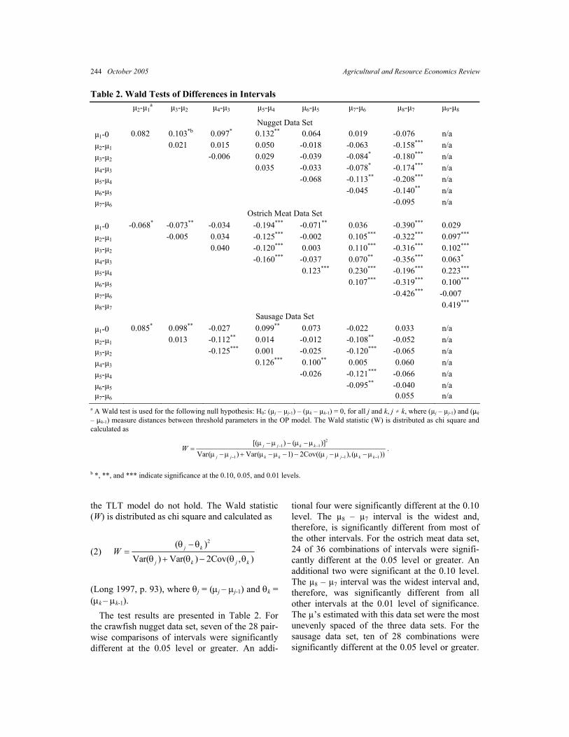
of 111 consumers who had been recruited by telephone in and around the city of Baton Rouge, Louisiana. Greater detail on the procedures is found in Harrison, Ozayan, and Meyers 1998). The second data set was collected to examine retailer preferences of ostrich meat products. Four attributes and their levels were selected: portion size, including non-portioned, four-ounce, and six-ounce portions; product type, including ground, processed, and filet; whether or not the product was branded; and purchase price from the processor in dollars per pound: $4.00, $8.00, and $12.00. A full factorial experimental design would involve 54 hypothetical product combina-tions. A fractional factorial design reduced the number of profiles to nine. The questionnaire was administered via mail to retailers in the south-central United States. Respondents were asked to rate each profile from 0 to 10, where 0 was the least and 10 the most preferred product. Conjoint results were collected from 133 retail outlets. See Gillespie et al. (1998) for greater detail on the study. The third data set was collected to examine consumer preferences of crawfish sausage prod-ucts. Four attributes and their respective levels were selected: price, which included $3.00 and $3.50 per pound levels; package size, which in-cluded 16- and 48-ounce sizes; cooking method, which included baked, pan fried, and deep fried; and product form, which included short, medium, and long sausage links. A full factorial experi-mental design would involve 36 hypothetical product combinations. A fractional factorial de-sign reduced the number of profiles to nine. The questionnaire was administered via personal in-terview. Respondents were asked to rate each profile from 1 to 10, where 1 was the least pre-ferred and 10 the most preferred product. Con-joint results were collected from 144 consumers. See Harrison, Stringer, and Prinyawiwatkul (2002) for greater detail on the study. Results A Wald statistic is used to test the following null hypothesis: H0: (µj – µj-1) – (µk – µk-1) = 0, for all j and k, j … k, where (µj – µj-1) and (µk – µk-1) meas-ure the interval distances between threshold pa-rameters in the OP model. Rejection of H0 pro-vides evidence that equal interval assumptions of


Table 2. Wald Tests of Differences in Intervals µ2-µ1

a µ3-µ2 µ4-µ3 µ5-µ4 µ6-µ5 µ7-µ6 µ8-µ7 µ9-µ8

Nugget Data Set µ1-0 0.082 0.103*b 0.097* 0.132** 0.064 0.019 -0.076 n/a µ2-µ1 0.021 0.015 0.050 -0.018 -0.063 -0.158*** n/a µ3-µ2 -0.006 0.029 -0.039 -0.084* -0.180*** n/a µ4-µ3 0.035 -0.033 -0.078* -0.174*** n/a µ5-µ4 -0.068 -0.113** -0.208*** n/a µ6-µ5 -0.045 -0.140** n/a µ7-µ6 -0.095 n/a

Ostrich Meat Data Set µ1-0 -0.068* -0.073** -0.034 -0.194*** -0.071** 0.036 -0.390*** 0.029 µ2-µ1 -0.005 0.034 -0.125*** -0.002 0.105*** -0.322*** 0.097***

µ3-µ2 0.040 -0.120*** 0.003 0.110*** -0.316*** 0.102***

µ4-µ3 -0.160*** -0.037 0.070** -0.356*** 0.063*

µ5-µ4 0.123*** 0.230*** -0.196*** 0.223***

µ6-µ5 0.107*** -0.319*** 0.100***

µ7-µ6 -0.426*** -0.007 µ8-µ7 0.419***

Sausage Data Set µ1-0 0.085* 0.098** -0.027 0.099** 0.073 -0.022 0.033 n/a µ2-µ1 0.013 -0.112** 0.014 -0.012 -0.108** -0.052 n/a µ3-µ2 -0.125*** 0.001 -0.025 -0.120*** -0.065 n/a µ4-µ3 0.126*** 0.100** 0.005 0.060 n/a µ5-µ4 -0.026 -0.121*** -0.066 n/a µ6-µ5 -0.095** -0.040 n/a µ7-µ6 0.055 n/a

a A Wald test is used for the following null hypothesis: H0: (µj – µj-1) – (µk – µk-1) = 0, for all j and k, j … k, where (µj – µj-1) and (:k

– :k-1) measure distances between threshold parameters in the OP model. The Wald statistic (W) is distributed as chi square and calculated as

21 1

1 1

[( ) ( )]Var( ) Var( 1) 2Cov(( ), ( ))

j j k k

j j k k j j k k

W − −

− −

µ −µ − µ −µ=

µ −µ + µ −µ − − µ −µ µ −µ 1−

.

b *, **, and *** indicate significance at the 0.10, 0.05, and 0.01 levels.

the TLT model do not hold. The Wald statistic (W) is distributed as chi square and calculated as

(2) 2( )

Var( ) Var( ) 2Cov( , )j k

j k j

Wθ − θ

=θ + θ − θ θk

(Long 1997, p. 93), where θj = (µj – µj-1) and θk = (µk – µk-1). The test results are presented in Table 2. For the crawfish nugget data set, seven of the 28 pair-wise comparisons of intervals were significantly different at the 0.05 level or greater. An addi-

tional four were significantly different at the 0.10 level. The µ8 – µ7 interval is the widest and, therefore, is significantly different from most of the other intervals. For the ostrich meat data set, 24 of 36 combinations of intervals were signifi-cantly different at the 0.05 level or greater. An additional two were significant at the 0.10 level. The µ8 – µ7 interval was the widest interval and, therefore, was significantly different from all other intervals at the 0.01 level of significance. The µ’s estimated with this data set were the most unevenly spaced of the three data sets. For the sausage data set, ten of 28 combinations were significantly different at the 0.05 level or greater.


Table 3. Two-Limit Tobit and Ordered Probit Part-Worth Estimates for the Nugget-Based Crawfish Products Analysis

TLT and OP

Index Function Estimates

OP Threshold Estimates

TLT and OP Standardized Estimates a

Attribute βTLT βOP µ βSTLT βS

OP βSTLT – βS

OP

Constant 0.646 (1.047)

0.146(0.240)

µ1 0.422(9.396)

*** 0.193 0.130 0.063

Average rating 1.145 (9.522)

***b 0.383(7.873)

*** µ2 0.762(14.223)

*** 0.342 0.340 -0.002

Packaging 0.010 (1.556)

0.003(1.492)

µ3 1.081(18.441)

*** 0.003 0.003 -0.000

Price -6.046 (-10.676)

*** -2.044(-10.275)

*** µ4 1.405(22.585)

*** -1.805 -1.815 0.010

Nugget form

-0.411 (-3.023)

*** -0.137(-2.976)

*** µ5 1.695(26.072)

*** -0.123 -0.121 0.001

Patty form 0.841 (6.214)

*** 0.283(5.799)

*** µ6 2.053(30.076)

*** 0.251 0.251 -0.001

Fried reheat -0.378 (-2.786)

*** -0.129(-2.816)

*** µ7 2.456(33.781)

*** -0.112 -0.114 0.001

Microwave reheat 0.400 (2.952)

*** 0.138(2.913)

*** µ8 2.954(37.264)

*** 0.119 0.123 -0.003

σ 2.974 (38.126)

*** 1

Log L. ratio χ2 229.78 *** 227.37 ***

Pseudo R2 .21 .21

Hausman statistic c 7.17 a The notation βS

TLT and βSOP refers to the standardized estimates, which are calculated using the following formula: s

kβ = βk /σy*, where σy* is the unconditional standard deviation of y* and is estimated by 2

*yσ = β′Var(x)β + Var(ε). b *, **, and *** indicate significance at the 0.10, 0.05, and 0.01 levels. c Hausman’s procedure is used to test the null hypothesis that TLT standardized estimates are inconsistent relative to OP standard-ized estimates. The Hausman statistic is distributed as chi square and defined as follows:

1OP TLT OP TLT OP TLT( ) '[Var( ) Var( )] (S S S S S SH −= β − β β − β β −β ) .

An additional one was significantly different at the 0.10 level. Each of these analyses showed significant differences in the intervals between the µ’s, suggesting that the equal interval assump-tion of the TLT model does not hold for any of the three data sets.

Comparison of Part-Worth Estimates

Given that equal interval assumptions of the TLT model do not hold for any of the data sets, it is useful to determine whether part-worth estimates differ between the two models. The index func-tion estimates for the TLT and OP models are

presented in Tables 3, 4, and 5 for the crawfish nugget, ostrich meat, and crawfish sausage data sets, respectively. The index function βs represent the part-worth estimates utilized in all of the pre-viously cited CA studies. For both models, the βs are interpreted as the change in the underlying utility scale given a unit change in x. Casual ob-servation of the results suggests that estimates of the TLT and OP analyses are consistent in the sense that, in all cases, the signs are the same, and variables that are significant for the TLT model are also significant for the OP model. However, since parameters in the TLT and OP models are


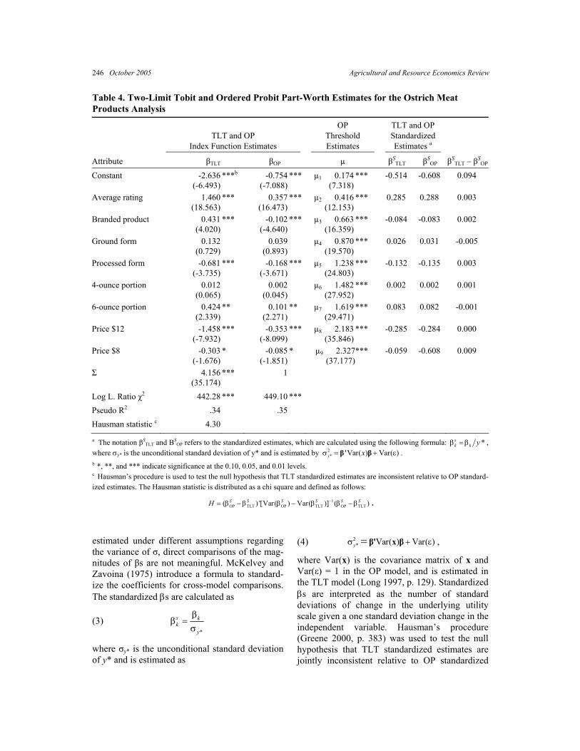
Table 4. Two-Limit Tobit and Ordered Probit Part-Worth Estimates for the Ostrich Meat Products Analysis

TLT and OP





OP βSTLT – βS

OP

Constant -2.636(-6.493)

***b -0.754(-7.088)

*** µ1 0.174(7.318)

*** -0.514 -0.608 0.094


*** 0.357(16.473)

*** µ2 0.416(12.153)

*** 0.285 0.288 0.003

Branded product 0.431 (4.020)

*** -0.102(-4.640)

*** µ3 0.663(16.359)

*** -0.084 -0.083 0.002

Ground form 0.132 (0.729)

0.039(0.893)

µ4 0.870(19.570)

*** 0.026 0.031 -0.005

Processed form -0.681 (-3.735)

*** -0.168(-3.671)

*** µ5 1.238(24.803)

*** -0.132 -0.135 0.003

4-ounce portion 0.012 (0.065)

0.002(0.045)

µ6 1.482(27.952)

*** 0.002 0.002 0.001

6-ounce portion 0.424 (2.339)

** 0.101(2.271)

** µ7 1.619(29.471)

*** 0.083 0.082 -0.001

Price $12 -1.458 (-7.932)

*** -0.353(-8.099)

*** µ8 2.183(35.846)

*** -0.285 -0.284 0.000

Price $8 -0.303 (-1.676)

* -0.085(-1.851)

* µ9 2.327(37.177)

*** -0.059 -0.608 0.009

Σ 4.156(35.174)

*** 1

Log L. Ratio χ2 442.28 *** 449.10 *** Pseudo R2 .34 .35 Hausman statistic c 4.30

a The notation βSTLT and ΒS

OP refers to the standardized estimates, which are calculated using the following formula: *sk k yβ = β ,

where σy* is the unconditional standard deviation of y* and is estimated by 2* 'Var( ) Var( )y xσ = +β β ε

)

. b *, **, and *** indicate significance at the 0.10, 0.05, and 0.01 levels. c Hausman’s procedure is used to test the null hypothesis that TLT standardized estimates are inconsistent relative to OP standard-ized estimates. The Hausman statistic is distributed as a chi square

and

defined as follows:

1OP TLT OP TLT OP TLT( ) '[Var( ) Var( )] (S S S S S SH −= β −β β − β β −β .

estimated under different assumptions regarding the variance of σ, direct comparisons of the mag-nitudes of βs are not meaningful. McKelvey and Zavoina (1975) introduce a formula to standard-ize the coefficients for cross-model comparisons. The standardized βs are calculated as

(3) *

s kk

y

ββ =

σ

where σy* is the unconditional standard deviation of y* and is estimated as

(4) 2* Var( ) Var( )yσ + ε= β' x β ,

where Var(x) is the covariance matrix of x and Var(ε) = 1 in the OP model, and is estimated in the TLT model (Long 1997, p. 129). Standardized βs are interpreted as the number of standard deviations of change in the underlying utility scale given a one standard deviation change in the independent variable. Hausman’s procedure (Greene 2000, p. 383) was used to test the null hypothesis that TLT standardized estimates are jointly inconsistent relative to OP standardized


Table 5. Two-Limit Tobit and Ordered Probit Part-Worth Estimates for the Crawfish Sausage Products Analysis

TLT and OP





OP βSTLT – βS

OP

Constant 2.736(2.192)

**b 0.813(1.955)

* µ1 0.392(10.282)

*** 0.714 0.654 -0.060


*** 0.426(17.167)

*** µ2 0.700(15.040)

*** 0.341 0.343 0.002

Price -1.026(-2.724)

*** -0.334(-2.669)

*** µ3 0.994(19.430)

*** -0.268 -0.269 -0.001

Package size -0.035 (-5.961)

*** -0.011(-5.741)

*** µ4 1.414(25.032)

*** -0.009 -0.009 -0.000

Link size: long 0.385 (3.058)

*** 0.126(3.098)

*** µ5 1.708(28.883)

*** 0.101 0.101 0.001

Link size: medium 0.390 (3.119)

*** 0.127(3.023)

*** µ6 2.027(32.836)

*** 0.102 0.103 0.001

Baked 0.955(7.612)

*** 0.312(7.806)

*** µ7 2.442(37.868)

*** 0.249 0.252 0.002

Deep fried 1.010 (8.072)

*** 0.329(7.780)

*** µ8 2.801(41.421)

*** 0.264 0.265 0.001

σ 3.091(40.927)

*** 1

Log L. Ratio χ2 522.91 *** 522.84 ***

Pseudo R2 .34 .35

Hausman statistic c 6.13

a The notation βSTLT and βS

OP refers to the standardized estimates, which are calculated using the following formula: , where σ

*/sk k yβ = β σ

y* is the unconditional standard deviation of y* and is estimated by 2* 'Var( ) Var( )y xσ = +β β ε

)

)i

. b *, **, and *** indicate significance at the 0.10, 0.05, and 0.01 levels. c Hausman’s procedure is used to test the null hypothesis that TLT standardized estimates are inconsistent relative to OP standard-ized estimates. The Hausman statistic is distributed as a chi square

and

defined as follows:

1

OP TLT OP TLT OP TLT( ) '[Var( ) Var( )] (S S S S S SH −= β −β β − β β −β . estimates. Results show that the standardized TLT estimates are not significantly different from the OP standardized estimates at the 0.10 level of significance (Tables 3, 4, and 5). Thus, despite rejection of the equal interval assumption, the two models do not differ significantly with respect to their estimates of the underlying utility scale. Analysis of Predicted Values Although the estimated TLT and OP models are consistent with respect to estimation of the under-lying utility index, predicted values of the two

models differ. Since there is no conditional mean for y in the OP model, the predicted value is the category having the highest probability of occur-rence, given x. Consequently, the spacing of the µ’s has a significant effect on predicted values of the OP model. Predicted values are calculated as (5) , 1

ˆ ˆ ˆ ˆ ˆ[ | ] ( ) (j j i jMax Pr y j u −= = Φ − −Φ µ −x x β x β

where ^ denotes the maximum likelihood estimates (Long 1997). (For simplification, ^ is dropped in the following discussion.) Since the conditional mean of y* (i.e., xiβ) is common


-2 -1 0 1 2

11'µ 2

'µ0'µ 3

'µ 4'µ 5

'µ 6'µ 7

'µ 8'µPr[ * | ]jy ≤µ x ( |j −Φµ βx x

|j −µ βx x

a

0

b

)

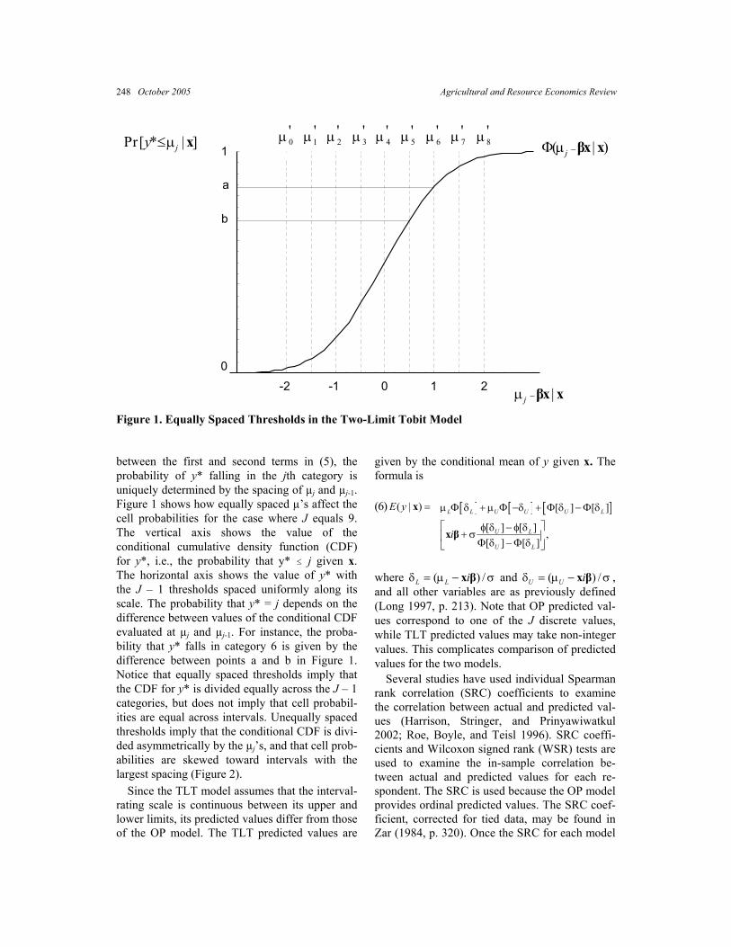
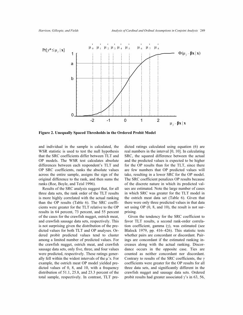
Figure 1. Equally Spaced Thresholds in the Two-Limit Tobit Model between the first and second terms in (5), the probability of y* falling in the jth category is uniquely determined by the spacing of µj and µj-1. Figure 1 shows how equally spaced µ’s affect the cell probabilities for the case where J equals 9. The vertical axis shows the value of the conditional cumulative density function (CDF) for y*, i.e., the probability that y* # j given x. The horizontal axis shows the value of y* with the J – 1 thresholds spaced uniformly along its scale. The probability that y* = j depends on the difference between values of the conditional CDF evaluated at µj and µj-1. For instance, the proba-bility that y* falls in category 6 is given by the difference between points a and b in Figure 1. Notice that equally spaced thresholds imply that the CDF for y* is divided equally across the J – 1 categories, but does not imply that cell probabil-ities are equal across intervals. Unequally spaced thresholds imply that the conditional CDF is divi-ded asymmetrically by the µj’s, and that cell prob-abilities are skewed toward intervals with the largest spacing (Figure 2). Since the TLT model assumes that the interval-rating scale is continuous between its upper and lower limits, its predicted values differ from those of the OP model. The TLT predicted values are

given by the conditional mean of y given x. The formula is (6) [ ] [ ] [ ]( | ) [ ] [ ]

[ ] [ ] ,[ ] [ ]

L L U U U L

U L

U L

E y

i

= µ Φ δ + µ Φ −δ + Φ δ −Φ δ

⎡ ⎤φ δ − φ δ+ σ⎢ ⎥Φ δ −Φ δ⎣ ⎦

x

x β

where ( )L L i /δ = µ − σx β and , and all other variables are as previously defined (Long 1997, p. 213). Note that OP predicted val-ues correspond to one of the J discrete values, while TLT predicted values may take non-integer values. This complicates comparison of predicted values for the two models.

( )U U iδ = µ − σx β /

Several studies have used individual Spearman rank correlation (SRC) coefficients to examine the correlation between actual and predicted val-ues (Harrison, Stringer, and Prinyawiwatkul 2002; Roe, Boyle, and Teisl 1996). SRC coeffi-cients and Wilcoxon signed rank (WSR) tests are used to examine the in-sample correlation be-tween actual and predicted values for each re-spondent. The SRC is used because the OP model provides ordinal predicted values. The SRC coef-ficient, corrected for tied data, may be found in Zar (1984, p. 320). Once the SRC for each model


1'µ 2

'µ0'µ 3

'µ 4'µ 5

'µ 6'µ 7

'µ 8'µ

-2 -1 0 1 2

1Pr[ * | ]jy ≤µ x

( | )j −Φ µ βx x

|j −µ βx x

a

b

0

Figure 2. Unequally Spaced Thresholds in the Ordered Probit Model and individual in the sample is calculated, the WSR statistic is used to test the null hypothesis that the SRC coefficients differ between TLT and OP models. The WSR test calculates absolute differences between each respondent’s TLT and OP SRC coefficients, ranks the absolute values across the entire sample, assigns the sign of the original difference to the rank, and then sums the ranks (Roe, Boyle, and Teisl 1996). Results of the SRC analysis suggest that, for all three data sets, the rank order of the TLT results is more highly correlated with the actual ranking than the OP results (Table 6). The SRC coeffi-cients were greater for the TLT relative to the OP results in 64 percent, 73 percent, and 55 percent of the cases for the crawfish nugget, ostrich meat, and crawfish sausage data sets, respectively. This is not surprising given the distribution of the pre-dicted values for both TLT and OP analyses. Or-dered probit predicted values tend to cluster among a limited number of predicted values. For the crawfish nugget, ostrich meat, and crawfish sausage data sets, only five, three, and four values were predicted, respectively. These ratings gener-ally fell within the widest intervals of the µ’s. For example, the ostrich meat OP model yielded pre-dicted values of 0, 8, and 10, with a frequency distribution of 51.1, 25.8, and 23.3 percent of the total sample, respectively. In contrast, TLT pre-

dicted ratings calculated using equation (6) are real numbers in the interval [0, 10]. In calculating SRC, the squared difference between the actual and the predicted values is expected to be higher for the OP results than for the TLT, since there are few numbers that OP predicted values will take, resulting in a lower SRC for the OP model. The SRC coefficient penalizes OP results because of the discrete nature in which its predicted val-ues are estimated. Note the large number of cases in which SRC was greater for the TLT model in the ostrich meat data set (Table 6). Given that there were only three predicted values in that data set using OP (0, 8, and 10), the result is not sur-prising. Given the tendency for the SRC coefficient to favor TLT results, a second rank-order correla-tion coefficient, gamma (γ), was estimated (see Blalock 1979, pp. 416–426). This statistic tests whether pairs are concordant or discordant. Pair-ings are concordant if the estimated ranking in-creases along with the actual ranking. Discor-dance occurs in the opposite case. Ties are counted as neither concordant nor discordant. Contrary to results of the SRC coefficients, the γ coefficients were greater for the OP results for all three data sets, and significantly different in the crawfish nugget and sausage data sets. Ordered probit results had greater associated γ’s in 63, 56,


Table 6. Results of the Spearman and Gamma Analyses

Median Value Number of Cases Wilcoxon Signed Rank Test b

Ordered Probit

Two-Limit Tobit TLT > OP OP > TLT Z-Value Probability

Crawfish nugget 0.35 0.38 71 40 -2.857*** c 0.004 Spearman rs a

Crawfish nugget 0.31 0.28 40 69 3.326*** 0.001 Gamma γ

Ostrich meat 0.32 0.43 74 28 -4.996*** 0.000 Spearman rs

Ostrich meat 0.43 0.39 43 54 0.810 0.418 Gamma γ

Sausage 0.58 0.62 76 61 -2.190** 0.028 Spearman rs

Sausage 0.67 0.52 40 94 4.584*** 0.000 Gamma γ

a Spearman rank correlation and gamma coefficients are calculated between actual and predicted rankings for each respondent in the sample. b The Wilcoxon signed rank test tests the null hypothesis that differences between Spearman rank and gamma values for TLT and OP models are equal to zero. c *, **, and *** indicate significance at the 0.10, 0.05, and 0.01 levels. and 70 percent of the cases for the crawfish nug-get, ostrich meat, and crawfish sausage data sets, respectively. This suggests greater concordance with the OP rankings than with the TLT rankings. Unfortunately, dependence on γ for determination of rank-order correlation has problems as well. Consider a hypothetical case where the actual ranking for a set of 10 profiles is 1, 2, 3, 4, 5, 6, 7, 8, 9, and 10, compared to TLT model predicted values of 1, 2, 3, 4, 5, 6, 7.51, 7.49, 9, and 10, and OP model predicted values of 1, 1, 1, 1, 1, 1, 1, 5, 5, and 10. In this case, γ = 0.96 for TLT pre-dicted values and 1 for OP predicted values. Though TLT values are more closely aligned with the actual results, they are not in complete con-cordance. While OP predicted values generally differ greatly from actual values, they are in con-cordance. These results suggest that neither SRC nor γ coefficients are entirely suitable for com-parison of predicted values across the TLT and OP models. Moreover, Kendall’s J coefficient suffers from similar problems as the estimation is also based upon concordance. The validity of using such techniques to compare the two models is questionable, leading us to depend upon tests

of differences in the index values for both mod-els, as was done earlier in the paper. Conclusions

Conjoint analysis (CA) has increased in popular-ity among agricultural economists in recent years. The technique has been used to estimate con-sumer preferences for a variety of new food prod-ucts, to analyze consumer preferences for food safety attributes, and to estimate consumers’ will-ingness-to-pay for recreational services. An im-portant methodological question among these stud-ies is whether interval-rating scales capture cardi-nal information, which has implications for model selection. This paper develops formal procedures for testing cardinal and ordinal assumptions in conjoint analysis. Theoretical concepts of equal interval and ordinal scaling are linked to the un-derlying assumptions of the TLT and OP models. The paper shows how an OP model can be used to test the equal interval assumptions of the TLT model. The analysis involves using Wald proce-dures to test the null hypothesis of equally spaced thresholds in the OP model. The null hypothesis


was tested and rejected for three separate conjoint data sets, implying that the underlying cardinality assumption of the TLT model is invalid for these samples. Therefore, we conclude that the OP model is the theoretically correct model for estimating part-worth parameters for these samples. However, the equal-interval assumption may hold for other studies given different experimental conditions. Since the TLT model is often used in the agri-cultural economics literature to estimate part-worth values, the effects of model misspecifica-tion are examined by analyzing index function parameters. Casual inspection of the standardized part-worth parameters showed little difference between the TLT and OP models. Moreover, the Hausman null hypothesis was rejected for all three data sets, indicating that TLT part-worth estimates are not statistically different from the OP estimates. Therefore, despite rejection of the equal interval assumptions of the TLT model, the models yield virtually identical estimates of the underlying utility scale. This implies that the TLT model provides a close approximation of the theoretically correct OP model, and that the TLT estimates are not particularly sensitive to the car-dinality assumption. This is an important finding since estimating the underlying utility scale is the central focus of most CA studies. Additionally, in studies where degrees of freedom are constrained, the TLT model may be preferable since it gener-ally requires fewer degrees of freedom for estima-tion. This is particularly relevant for studies that estimate individual-level models. Unlike the analysis of index function parame-ters, comparisons of predicted values for the two models lead to inconclusive results. The two models yield conceptually different predictions for the observed interval-rating scale. The TLT model assumes equal spacing and continuity of the observed scale, thus yielding non-integer pre-dictions. The OP model assumes ordinal spacing of the observed scale, thus yielding discrete pre-dictions that result in numerous ties between ac-tual and predicted values. Moreover, comparison of predicted values using standard techniques for analyzing rank-order data, such as SRC coeffi-cients, γ, and Kendall’s τ, are invalid. Spearman’s rank-order coefficient favors the TLT model be-cause of the non-integer nature of its predictions, whereas γ and Kendall’s τ favor the OP model because they measure the degree of concordance.

Our general conclusion is that, while modern economic theory and the empirical rejection of equal-interval cardinality suggest that the OP is theoretically superior to the TLT model, re-searchers relying upon part-worth estimates from conjoint analyses are unlikely to find significant differences in the part-worth estimates between the two models. Theory leads to recommendation of the OP model, while empirical evidence sug-gests that, in estimating part-worth utilities, either can be used. In cases where there are too few degrees of freedom to estimate an OP model, the TLT is likely to be the best option. The similarity in model estimates also implies that utility esti-mates are not particularly sensitive to assump-tions regarding interpersonal comparisons. In fact, if one carefully plans the conjoint design, there are often enough degrees of freedom to es-timate individual preference functions using the TLT model, which avoids the pooling of individ-ual preferences altogether. Individual estimates are usually not possible with the OP model. References Alchian, A.A. 1953. “The Meaning of Utility Measurement.”

American Economic Review 43(1): 26–50. Baker, G.A., and P.J. Crosbie. 1993. “Measuring Food Safety

Preferences: Identifying Consumer Segments.” Journal of Agricultural and Resource Economics 18(2): 277–287.

Blalock, H.M. 1979. Social Statistics. New York: McGraw-Hill.

Boyle, K., T.P. Holmes, M. Teisl, and B. Roe. 2001. “A Com-parison of Conjoint Analysis Response Formats.” American Journal of Agricultural Economics 83(2): 441–454.

Dennis, D.F. 1998. “Analyzing Public Inputs to Multiple Objective Decisions on National Forests Using Conjoint Analysis.” Forest Science 44(3): 421–429.

Fisher, I. 1918. “Is Utility the Most Suitable Term for the Concept It Is Used to Denote?” American Economic Review 8(2): 335–337.

Gan, C., and E.J. Luzar. 1993. “A Conjoint Analysis of Water-fowl Hunting in Louisiana.” Journal of Agricultural and Applied Economics 25(2): 36–45.

Gillespie, J., G. Taylor, A. Schupp, and F. Wirth. 1998. “Opin-ions of Professional Buyers Toward a New, Alternative Red Meat: Ostrich.” Agribusiness 14(3): 247–256.

Gineo, W.M. 1990. “A Conjoint/Logit Analysis of Nursery Stock Purchases.” Northeastern Journal of Agricultural and Resource Economics 19(1): 49–61.

Greene, W.H. 2000. Econometric Analysis. Englewood Cliffs, NJ: Prentice Hall.


Halbrendt, C.K., R.J. Bacon, and J. Pesek. 1992 . “Weighted Least Squares Analysis for Conjoint Studies: The Case of Hybrid Striped Bass.” Agribusiness 8(2): 187–198.

Halbrendt, C.K., F.F. Wirth, and G.F. Vaughn. 1991. “Con-joint Analysis of the Mid-Atlantic Food-Fish Market for Farm-Raised Hybrid Striped Bass.” Southern Journal of Agricultural Economics 23(1): 155–163.

Harrison, R.W., A. Ozayan, and S.P. Meyers. 1998. “A Con-joint Analysis of New Food Products Processed from Un-derutilized Small Crawfish.” Journal of Agricultural and Applied Economics 30(2): 257–265.

Harrison, R.W, T. Stringer, and W. Prinyawiwatkul. 2002. “An Analysis of Consumer Preferences for Value-Added Seafood Products Derived from Crawfish.” Agricultural and Resource Economics Review 31(2): 157–170.

Henderson, J.M., and R. Quandt. 1980. Microeconomic The-ory. New York: McGraw-Hill.

Hobbs, J.E. 1996. “Transaction Costs and Slaughter Cattle Procurement: Processors Selection of Supply Channels.” Agribusiness 12(6): 509–523.

Holland, D., and C.R. Wessells. 1998. “Predicting Consumer Preferences for Fresh Salmon: The Influence of Safety In-spection and Production Method Attributes.” Agricultural and Resource Economics Review 27(1): 1–14.

Jevons, W.S. 1871. The Theory of Political Economy. London: McMillan.

Lin, B.H., S. Payson, and J. Wertz. 1996. “Opinions of Profes-sional Buyers Toward Organic Produce: A Case Study of Mid-Atlantic Market for Fresh Tomatoes.” Agribusiness 12(1): 89–97.

Long, J.S. 1997. Regression Models for Categorical and Lim-ited Dependent Variables. Thousand Oaks, CA: SAGE Publications.

Mackenzie, J. 1990. “Conjoint Analysis of Deer Hunting.” Northeastern Journal of Agricultural and Resource Eco-nomics 19(2): 109–117.

____. 1993. “A Comparison of Contingent Preference Mod-els.” American Journal of Agricultural Economics 75(3): 593–603.

McKelvey, M.D., and W. Zavoina. 1975. “A Statistical Model for the Analysis of Ordinal Level Dependent Variables.” Journal of Mathematics and Sociology 4(1): 103–119.

Menger, C. 1981. Principles of Economics (translated by J. Dingwald and B.F. Hoselitz). New York: New York Uni-versity Press.

Miquel, F.S., M. Ryan, and E. McIntosh. 2000. “Applying Conjoint Analysis in Economic Evaluation: An Application to Menorrhagia.” Applied Economics 32(7): 823–837.

Pareto, V. 1909. Manuel d’Economie Politique. Paris: V. Giard and E. Buere.

Prentice, B.E., and D. Benell. 1992.”Determinants of Empty Returns by U.S. Refrigerated Trucks: Conjoint Analysis

Approach.” Canadian Journal of Agricultural Economics 40(1): 109–127.

Reddy, V.S., and R.J. Bush. 1998. “Measuring Softwood Lumber Value: A Conjoint Analysis Approach.” Forest Science 44(1): 145–157.

Robbins, L. 1932. An Essay on the Nature and Significance of Economic Science. London: McMillan.

Roe, B., K.J. Boyle, and M.F. Teisl. 1996. “Using Conjoint Analysis to Derive Estimates of Compensating Variation.” Journal of Environmental Management 31(2): 145–159.

Silberberg, E. 1978. The Structure of Economics. New York: McGraw-Hill.

Stevens, T.H., C. Barrett, and C.E. Willis. 1997. “Conjoint Analysis of Groundwater Protection Programs.” Agricul-tural and Resource Economics Review 26(2): 229–236.

Stevens, T.H., D. Dennis, D. Kittredge, and M. Rickenbach. 1999. “Attitudes and Preferences Toward Co-operative Agreements for Management of Private Forestlands in the Northeastern United States.” Journal of Environmental Management 55(2): 81–90.

Stigler, G.J. 1950. “The Development of Utility Theory I.” Journal of Political Economy 58(3): 307–327.

Swallow, S.K., J.J. Opaluch, and T.F. Weaver. 2001. “Strength-of-Preference Indicators and an Ordered-Response Model for Ordinarily Dichotomous, Discrete Choice Data.” Journal of Environmental Economics and Management 41(1): 70–93.

Sy, H.A., M.D. Faminow, G.V. Johnson, and G. Crow. 1997. “Estimating the Values of Cattle Characteristics Using an Ordered Probit Model.” American Journal of Agricultural Economics 79(2): 463–476.

Sylvia, G., and S.L. Larkin. 1995. “Firm-Level Intermediate Demand for Pacific Whiting Products: A Multi-Attribute, Multi-Sector Analysis.” Canadian Journal of Agricultural Economics 43(3): 501–518.

Torgerson, W.S. 1958. Theory and Methods of Scaling. New York: John Wiley & Sons, Inc.

van Praag, B.M.S. 1991. “Ordinal and Cardinal Utility.” Jour-nal of Econometrics 50(1): 69–89.

Varian, H.R. 1947. Microeconomic Analysis. Princeton, NJ: Princeton University Press.

von Neumann, J., and O. Morgenstern. 1947. Theory of Games and Economic Behavior (2nd edition). Princeton, NJ: Princeton University Press.

Yoo, D., and H. Ohta. 1995. “Optimal Pricing and Product-Planning for New Multiattribute Products Based on Con-joint Analysis.” International Journal of Production Eco-nomics 38(2): 245–253.

Zar, J.H. 1984. Biostatistical Analysis (2nd edition). Engle-wood Cliffs, NJ: Prentice-Hall.

analysis of cardinal and ordinal assumptions in conjoint...

Documents