analysis of covariance€¦ · · 2016-01-18an one-way analysis of variance confirms what was...

ANALYSIS OF COVARIANCE

Jesús Piedrafita Arilla [email protected]

Departament de Ciència Animal i dels Aliments

Experimental Design and Statistical Methods

Workshop

http://cran.r-project.org/index.html

Items

• Analysis of covariance

– Concept and assumptions

– One way ANOVA

– Plot of y vs covariate by groups

– Equality of variances

– Models

– Regression equation

– Predicted values

• Splitting observations according to treatment.

• lm

2

Analysis of covariance

Useful when the dependent variable is explained by both categorical and continuous independent variables. Common application of analysis of covariance is to adjust treatment means for a known source of variability

that can be explained by a continuous variable (covariate, xij). It is something like blocking, but for continuous variables.

The model of analysis is

ijiijij xy 10

The assumptions are:

1. The covariate is fixed and independent of treatments.

2. Errors are independent of each other.

3. Usually, errors have a normal distribution with mean 0 and homogeneous variance.

3

Analysis of covariance – the data (1) -

Two medicines (Fibralo and Gemfibrozil) were compared for the reduction of triglyceride levels in 34 diabetic non-insulin dependent patients.

The distribution of triglyceride reduction in both treatments is fairly homogeneous and close to normality.

No differences between treatments are evident.

4

Analysis of covariance – results (1) -

An one-way analysis of variance confirms what was suspected.

Not significant

> anova(aov(TRIGCHANGE~TRT))

Analysis of Variance Table

Response: TRIGCHANGE

Df Sum Sq Mean Sq F value Pr(>F)

TRT 1 327.2 327.22 1.1786 0.2858

Residuals 32 8884.5 277.64

> m<-tapply(TRIGCHANGE, TRT, length)

> p<-tapply(TRIGCHANGE, TRT, mean)

> r<-tapply(TRIGCHANGE, TRT, sd)

> cbind(N=m, Mean=p, Std.dev=r)

N Mean Std.dev

Fib 16 -4.06250 16.95275

Gem 18 -10.27778 16.40232

Observe the high within treatment variability. That masks possible differences between treatments.

5

5 6 7 8 9

-40

-30

-20

-10

010

20

HBA1C

TRIGCHANGE

Analysis of covariance – the data (2) -

As an indicator of the severity of diabetes, HbA1c was measured. This variable could be also related to the triglyceride change.

A clear negative relationship exists between triglyceride change and the severity of diabetes.

Circles and triangles indicate Fibralo and Gemfibrozil treatments, respectively.

Regression lines are quite parallel for the two treatments.

Fib

Gem

6

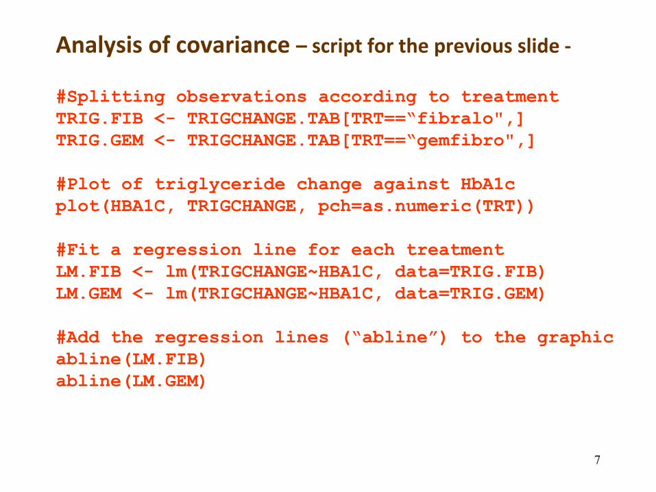
Analysis of covariance – script for the previous slide -

#Splitting observations according to treatment

TRIG.FIB <- TRIGCHANGE.TAB[TRT==“fibralo",]

TRIG.GEM <- TRIGCHANGE.TAB[TRT==“gemfibro",]

#Plot of triglyceride change against HbA1c

plot(HBA1C, TRIGCHANGE, pch=as.numeric(TRT))

#Fit a regression line for each treatment

LM.FIB <- lm(TRIGCHANGE~HBA1C, data=TRIG.FIB)

LM.GEM <- lm(TRIGCHANGE~HBA1C, data=TRIG.GEM)

#Add the regression lines (“abline”) to the graphic

abline(LM.FIB)

abline(LM.GEM)

7

> anova(lm(TRIGCHANGE~HBA1C*TRT))




HBA1C 1 5442.7 5442.7 57.4429 1.884e-08 ***

TRT 1 865.4 865.4 9.1331 0.005098 **

HBA1C:TRT 1 61.2 61.2 0.6458 0.427939

Residuals 30 2842.5 94.7


In the previous figure we can think about two different regression lines, one for each population. Is this meaningful?

Both the effects of the covariate (HbA1c) and the treatment were significant.

The interaction is not significant, so we can assume a common slope for the two treatments: regression lines are parallel. A simpler model can be fitted.

8

> anova(lm(TRIGCHANGE~HBA1C+TRT))




HBA1C 1 5442.7 5442.7 58.1068 1.353e-08 ***

TRT 1 865.4 865.4 9.2387 0.004783 **

Residuals 31 2903.7 93.7


We will assume a simplified model including only HBA1C as a covariate and the main effect of treatment.

The current model only includes the covariate and the treatment effect, both are significant.

Observe how the introduction of a covariate (the equivalent to blocking for a continuous variable) has reduced the Mean Sq to 93.7 from 277.64 of this statistic in the one-way anova –see a previous slide-. This makes the test more sensitive.

9

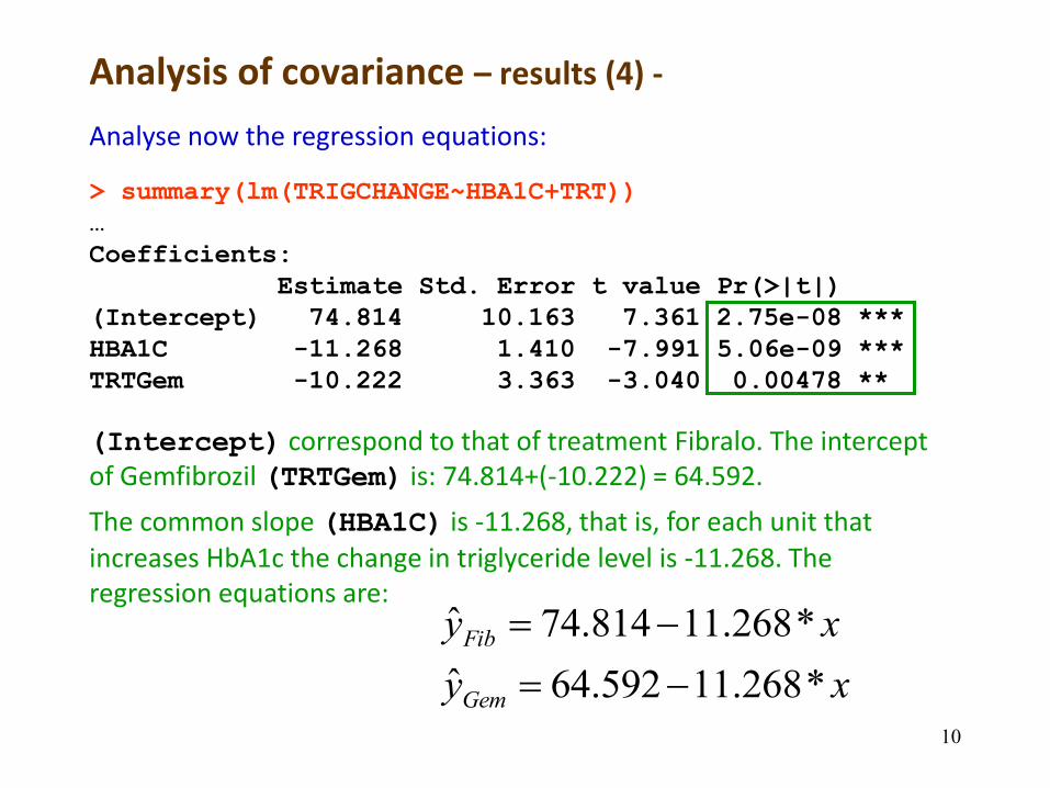
(Intercept) correspond to that of treatment Fibralo. The intercept of Gemfibrozil (TRTGem) is: 74.814+(-10.222) = 64.592.

The common slope (HBA1C) is -11.268, that is, for each unit that increases HbA1c the change in triglyceride level is -11.268. The regression equations are:

> summary(lm(TRIGCHANGE~HBA1C+TRT))

…

Coefficients:

Estimate Std. Error t value Pr(>|t|)

(Intercept) 74.814 10.163 7.361 2.75e-08 ***

HBA1C -11.268 1.410 -7.991 5.06e-09 ***

TRTGem -10.222 3.363 -3.040 0.00478 **


Analyse now the regression equations:

xy

xy

Gem

Fib

*268.11592.64ˆ

*268.11814.74ˆ

10

Analysis of covariance – results (4 cont) -

16.12812.6268.11592.64

94.1812.6268.11814.74

Gem

Fib

y

y

Analyse now the mean predicted values for TRIGCHANGE:

These predicted means are the means of TRIGCHANGE in each treatment if the people in them would had a value of 6.812 for HbA1c, i.e., the same level of severity of diabetes. This increases the sensitivity of the comparison.

We will summarize the results in the following table:

Fibralo Gemfibrozil p-value

Means -4.06 -10.28 NS

Pred. Means (covariate) -1.94 -12.16 **

6.812 is the mean of HbA1c in the total sample

11


Another way to compare the results of both models:

After adjusting for HBA1C, the difference between treatments become significant.

12

> library(multcomp)

> summary(glht(lm(TRIGCHANGE~TRT), linfct=mcp (TRT="Tukey")))

Linear Hypotheses:


gemfibro - fibralo == 0 -6.215 5.725 -1.086 0.286

> summary(glht(lm(TRIGCHANGE~HBA1C+TRT), linfct=mcp

(TRT="Tukey")))

Linear Hypotheses:


gemfibro - fibralo == 0 -10.222 3.363 -3.04 0.00478 **

---

Signif. codes: 0 ‘***’ 0.001 ‘**’ 0.01 ‘*’ 0.05 ‘.’ 0.1 ‘ ’ 1

(Adjusted p values reported -- single-step method)

analysis of covariance€¦ · · 2016-01-18an one-way analysis of variance confirms what was...

Documents