analysis of covariance - stern.nyu.edujsimonof/classes/2301/pdf/ancova.pdf · analysis of...
TRANSCRIPT

Analysis of covariance
Analysis of variance (ANOVA) models are restrictive in that they allow only categori-
cal predicting variables. Analysis of covariance (ANCOVA) models remove this restriction
by allowing both categorical predictors (often called grouping variables or factors) and
continuous predictors (typically called covariates) in the model. So, for example, in the
mileage of automobiles example, potential predictors of miles per gallon could be size and
year of the auto (grouping variables), and also the weight and engine size of the auto
(covariates).
The standard ANCOVA model incorporates covariates into an ANOVA model in a
straightforward way. If there is one grouping variable, for example, the model is
yij = µ + αi + β1x1ij + · · · + βpxpij + εij ,
where αi is the corrected effect on y given that you are in group i (corrected in the sense
that the covariates x1, . . . ,xp are taken into account). This model is fit using K − 1 effect
codings to represent the grouping variable, along with the p covariates and the constant
term.
From this model, we have several hypotheses of interest:
(1) Are there differences in level between groups (given the covariates)? This tests the
null hypothesis
H0 : α1 = · · · = αK = 0.
The test used for this hypothesis is the partial F–test for the K − 1 effect coding
variables (that is, it is based on the residual sum of squares using all of the variables,
and the residual sum of squares using only the covariates).
(2) Do the covariates have any predictive power for y (given the grouping variable)? This
tests the null hypothesis
H0 : β1 = · · · = βp = 0.
The test used for this hypothesis is the partial F–test for the covariates (that is, it is
based on the residual sum of squares using all of the variables, and the residual sum
of squares using only the effect codings).
c© 2016, Jeffrey S. Simonoff 1

(3) Does the particular variable x` provide any predictive power given the grouping vari-
able and the other covariates? This tests the null hypothesis
H0 : β` = 0.
The test used for this hypothesis is the usual t–test for that covariate.
This model generalizes to more than one grouping variable as well. For two grouping
variables, for example, the model is
yijk = µ + αi + βj + (αβ)ij + γ1x1ijk + · · · + γpxpijk + εijk ,
which allows for two main effects (fit using effect codings for each grouping variable) and
an interaction effect (fit using the pairwise products of the effect codings for the main
effects), as well as the presence of covariates. (I’ve changed the slope coefficients for the
covariates to γ’s so that the earlier (α, β) notation used for two–way ANOVA can be used
here as well.) The usual ANOVA–type hypotheses about the significance of main effects
and the interaction effect are tested using the appropriate partial F–tests.
This regression approach is not always used by statistical packages; some use a cell
means approach instead, which can give different answers (usually only slightly different).
Many ANCOVA routines (including that of Minitab) are quite restrictive, being designed
for use only with balanced designs (and even then only giving approximate F–tests), so
I don’t recommend using them (the Minitab general linear model routine fits the exact
F–tests correctly).
Both models mentioned here are constant shift models, in the sense that the only
differences between the expected value of the target variable between groups is one of shift,
with the slopes of the covariates being the same no matter what group an observations falls
in. Indeed, the ANCOVA model with one grouping variable is identical to the constant shift
model that we’ve used before, except that more than two levels of the grouping variable is
allowed. This leads to a natural question: might the slopes also be different between levels
of the grouping variable? Of course, this is exactly the same as the question of whether
the full model is an improvement over the constant shift model, and it is tested the same
c© 2016, Jeffrey S. Simonoff 2

way. Assume for simplicity that there is one covariate x in the data. A generalized model
that allows for different slopes for different groups is
yij = µ + αi + β1ixij + εij ,
where β1i is the slope of x for the ith group. If the interaction of the grouping variable
and the covariate are entered as part of the general linear model, the partial F–test for
this set of variables is a test of the hypothesis
H0 : β11 = · · · = β1K
(this is often called a test of common slope). This is easily generalized to p > 1 covariates
using the appropriate interaction terms. Note that this model can only be fit if you have at
least p + 1 observations within each group (for example, in the simple regression situation
you need at least two observations in each group). This could also be generalized to the
situation with more than one grouping variable, but that is rarely done.
By the way, this is one way of deseasonalizing time series data. Say you have quarterly
data, and you want to regress a target variable on a set of predictors. You might think
that your target might exhibit a time trend, so you include time as a predictor in the
model (detrending). You also think that there might be seasonal effects in the data. You
can include those possible effects (that is, deseasonalize the data) by creating a variable
that defines the four quarters and then include it as a grouping variable in the general
linear model. The partial F–test for that effect is a test of a seasonal effect on level (for
example, the target is higher in the spring given the covariates, lower in the summer, etc.).
Even if this test is not significant, however, you might very well find that a significant
lag–4 autocorrelation (before deseasonalizing) that was indicating a seasonal effect is no
longer significant. For monthly data, you would use a variable defining the 12 months. For
weekly data, you can imagine using a variable with 52 levels, but that would require lots
of data to be reasonable.
c© 2016, Jeffrey S. Simonoff 3

Trade breaks on the exchange floor
When a customer calls a stock trading house to place an order to buy or sell stocks
listed on the New York Stock Exchange, the office contacts the trader, who goes to the
specialist booth and says “I want to buy x shares of XYZ at $10”. The trader writes the
order down on a piece of paper (“I bought x shares of XYZ at $10.”), and the person
at the booth also records the trade (“I sold x shares of XYZ at $10.”). This is called
executing the trade. The pieces of paper are later matched up (the matching process). If
the information on the pieces of paper doesn’t match, this is called a trade break. It is
labor intensive to resolve these breaks, as someone has to go back to the people involved
and ask questions, so it is important to the trading house to understand and control trade
breaks. The following data refer to all of the daily trades that occurred from June 1995
through May 1996 at a large New York City investment house (sorry, but I’m not allowed
to say which one). For each day the total number of trades (Trade Total), total number
of trade breaks (Trade Breaks), the percent of the trades the resulted in breaks (Break
Rate), and the day of the week are recorded. Is it possible to build a model that describes
and predicts break rates?
First, here are some descriptive statistics. The break rate is about 7.5%, which is
around the industry average. With an average of almost 3000 trades daily, this translates
into more than 200 trade breaks per day on average.
Descriptive Statistics
Variable N N* Mean Median Tr Mean StDev SE Mean
Total_Br 254 2 219.57 206.50 210.29 92.53 5.81
Trade_To 254 2 2996.6 2952.0 2992.5 695.6 43.6
Break_Ra 254 2 7.545 7.019 7.212 2.815 0.177
Variable Min Max Q1 Q3
Total_Br 79.00 1298.00 180.00 241.00
Trade_To 1057.0 5383.0 2570.2 3437.7
Break_Ra 3.674 28.496 6.141 8.233
c© 2016, Jeffrey S. Simonoff 4

A histogram of break rates strongly suggests a long right tail:
3020100
100
90
80
70
60
50
40
30
20
10
0
Break rate
Fre
qu
en
cy
We will therefore work in the log scale, although even for this variable there is a bit
of a long tail:
c© 2016, Jeffrey S. Simonoff 5

1.51.41.31.21.11.00.90.80.70.60.5
60
50
40
30
20
10
0
Logged break rate
Fre
qu
en
cy
Side–by–side boxplots give evidence of a day of the week effect on logged break rate,
with the middle days of the week having lower break rate. This suggests the possibility
of some sort of psychological (carelessness) effect related to being close to the weekend
(either looking forward to it or recovering from it!).
c© 2016, Jeffrey S. Simonoff 6

FridayThursdayWednesdayTuesdayMonday
1.5
1.4
1.3
1.2
1.1
1.0
0.9
0.8
0.7
0.6
0.5
Day of week
Lo
gg
ed
bre
ak r
ate
There also appears to be a relationship between logged break rate and the total number
of trades, with busier trading days associated with lower break rate. This is puzzling, as
we might expect a higher break rate on busy days. The explanation I was given is that on
days when volume is anticipated to be high, the traders are told to be particularly careful
in recording their trades. Another possibility is that the people who perform the matching
don’t want to work so hard, so on busier days they certify more trades as matched when
they actually weren’t. A third suggestion I’ve gotten is that breaks occur more often in
the morning; if on busy days trading gets heavier in the afternoon (when there is a lower
chance of a break), the percentage of trades broken for the day would go down. A fourth
suggestion is that on high volume days the traders are more likely to leave their slips with
the specialist and let him (or his clerk) write down the details of the trade; since it is all
internal to the specialist booth, there is less likelihood of mistakes. A fifth suggestion is
that on busy days the specialist acts as one side of the trade more often, leading to less
confusion and therefore fewer trade breaks.
c© 2016, Jeffrey S. Simonoff 7

1000 1500 2000 2500 3000 3500 4000 4500 5000 5500
0.5
0.6
0.7
0.8
0.9
1.0
1.1
1.2
1.3
1.4
1.5
Total number of trades
Lo
gg
ed
bre
ak r
ate
The regression model that relates the logged break rate to the day of the week and the
total number of trades is an ANCOVA model, with day of the week as a grouping variable
and trade total a covariate. Here is the ANCOVA output:
General Linear Model: Logged break rate versus Trade_Total,
Day of week
Method
Factor coding (-1, 0, +1)
Rows unused 2
Factor Information
Factor Type Levels Values
Day of week Fixed 5 Friday, Monday, Thursday, Tuesday,
Wednesday
c© 2016, Jeffrey S. Simonoff 8

Analysis of Variance
Source DF Adj SS Adj MS F-Value P-Value
Trade_Total 1 0.78921 0.789215 70.78 0.000
Day of week 4 0.18560 0.046401 4.16 0.003
Error 248 2.76508 0.011150
Lack-of-Fit 244 2.75395 0.011287 4.06 0.088
Pure Error 4 0.01113 0.002783
Total 253 3.76889
Model Summary
S R-sq R-sq(adj) R-sq(pred)
0.105591 26.63% 25.15% 22.36%
Coefficients
Term Coef SE Coef T-Value P-Value VIF
Constant 1.1004 0.0295 37.33 0.000
Trade_Total -0.000081 0.000010 -8.41 0.000 1.01
Day of week
Friday 0.0079 0.0132 0.60 0.549 1.61
Monday 0.0392 0.0137 2.86 0.005 1.67
Thursday 0.0146 0.0132 1.11 0.268 1.61
Tuesday -0.0350 0.0132 -2.64 0.009 1.62
Regression Equation
Day of week
Monday Logged break rate = 1.1395 -0.000081Trade_Total
Tuesday Logged break rate = 1.0654 -0.000081Trade_Total
Wednesday Logged break rate = 1.0736 -0.000081Trade_Total
Thursday Logged break rate = 1.1150 -0.000081Trade_Total
Friday Logged break rate = 1.1083 -0.000081Trade_Total
c© 2016, Jeffrey S. Simonoff 9

Means
Fitted
Term Mean SE Mean
Day of week
Monday 0.8977 0.0155
Tuesday 0.8235 0.0148
Wednesday 0.8318 0.0146
Thursday 0.8731 0.0147
Friday 0.8664 0.0147
Data
Covariate Mean StDev
Trade_Total 2997 696
Both the day of the week and the total number of trades are significant predictors for
logged break rate. The entries under Term show that given the day of the week there is an
inverse relationship between logged break rate and the total number of trades, with 100
additional trades associated with an increase in logged break rate of (100)(−.000081) =
−.0081. That is, 100 more total trades is associated with multiplying the break rate by
10−.0081 = .982, or a reduction of 1.8% (remember that this is a semilog model), given
the day of the week is held fixed. The entries under Means show that given the total
number of trades, break rates are lower in the middle of the week and particularly high
on Mondays (I guess those traders both work hard and play hard!). The difference in
fitted means between Monday and Tuesday, for example, is .8977 − .8235 = .0742, which
means that given that the total number of trades is the same, the expected break rate on
Monday is a multiplicative factor of 10.0742 = 1.186 higher than that on Tuesday (that is,
18.6% higher). We see that about one–quarter of the variability in logged break rates is
accounted for by the model.
The fitted means deserve further comment. The adjustment here refers to the fact
that these are estimated means for the days of the week given the covariate(s) (specifically,
they estimate the expected y if all covariates equal their mean value). These are not the
same as the ordinary means:
c© 2016, Jeffrey S. Simonoff 10

Descriptive Statistics
Variable Day of w N Mean Median Tr Mean
Logged b Monday 47 .9079 0.8807 0.8936
Tuesday 51 0.8264 0.8301 0.8228
Wednesda 52 0.8299 0.8203 0.8276
Thursday 52 0.8677 0.8438 0.8632
Friday 52 0.8615 0.8464 0.8506
Note, for example, that the fitted mean for Monday is slightly smaller than the or-
dinary (unadjusted) mean. This is because part of the high break rate on Mondays is
accounted for by the low average number of trades on that day (recall that there is an
inverse relationship between break rate and total number of trades). The overall pattern
is not very different between the adjusted and unadjusted means, however.
Since we are fitting a model that does not include an interaction, we can compare the
fitted means to see which days are significantly different from each other. Here are the
Tukey comparisons:
Comparisons for Logged break rate
Tukey Pairwise Comparisons: Response = Logged break rate,
Term = Day of week
Grouping Information Using the Tukey Method and 95% Confidence
Day of week N Mean Grouping
Monday 47 0.897660 A
Thursday 52 0.873103 A B
Friday 52 0.866389 A B
Wednesday 52 0.831783 B
Tuesday 51 0.823543 B
Means that do not share a letter are significantly different.
c© 2016, Jeffrey S. Simonoff 11

Tukey Simultaneous Tests for Differences of Means
Difference of Day of Difference SE of Simultaneous 95%
week Levels of Means Difference CI
Monday - Friday 0.0313 0.0213 (-0.0269, 0.0895)
Thursday - Friday 0.0067 0.0207 (-0.0498, 0.0632)
Tuesday - Friday -0.0428 0.0208 (-0.0997, 0.0140)
Wednesday - Friday -0.0346 0.0207 (-0.0911, 0.0219)
Thursday - Monday -0.0246 0.0213 (-0.0828, 0.0337)
Tuesday - Monday -0.0741 0.0214 (-0.1324, -0.0158)
Wednesday - Monday -0.0659 0.0213 (-0.1240, -0.0077)
Tuesday - Thursday -0.0496 0.0208 (-0.1064, 0.0073)
Wednesday - Thursday -0.0413 0.0207 (-0.0979, 0.0152)
Wednesday - Tuesday 0.0082 0.0208 (-0.0486, 0.0651)
Difference of Day of Adjusted
week Levels T-Value P-Value
Monday - Friday 1.47 0.585
Thursday - Friday 0.32 0.998
Tuesday - Friday -2.06 0.239
Wednesday - Friday -1.67 0.452
Thursday - Monday -1.15 0.779
Tuesday - Monday -3.47 0.005
Wednesday - Monday -3.09 0.017
Tuesday - Thursday -2.38 0.121
Wednesday - Thursday -1.99 0.268
Wednesday - Tuesday 0.40 0.995
Individual confidence level = 99.32%
We see that the important difference is the adjusted rate on Monday being much higher
than that on Tuesday and Wednesday.
Let’s check some assumptions. Here are residual plots and diagnostics (remember, the
model is based on 5 predictors, not 2):
c© 2016, Jeffrey S. Simonoff 12

Row Trade_Date Break_Rate SRES1 HI1 COOK1
1 6/1/95 7.5117 -0.15049 0.0199450 0.000077
2 6/2/95 5.5615 -1.30721 0.0197564 0.005740
3 6/5/95 24.8516 4.27566 0.0234331 0.073111
4 6/6/95 8.3578 1.26281 0.0212740 0.005777
5 6/7/95 5.5786 -0.70698 0.0193445 0.001643
6 6/8/95 6.2500 -0.87808 0.0197350 0.002587
7 6/9/95 7.4188 -0.01752 0.0193754 0.000001
8 6/12/95 7.5977 -0.34226 0.0213678 0.000426
9 6/13/95 6.4541 -0.45916 0.0208552 0.000748
10 6/14/95 6.1668 -0.33382 0.0192619 0.000365
11 6/15/95 10.2936 1.09845 0.0203740 0.004182
12 6/16/95 7.0064 -0.33156 0.0196726 0.000368
13 6/19/95 6.4072 -0.94339 0.0212861 0.003226
14 6/20/95 3.6739 -1.72460 0.0280829 0.014323
15 6/21/95 5.6180 -0.62609 0.0195115 0.001300
16 6/22/95 7.0009 0.02173 0.0200130 0.000002
17 6/23/95 6.4358 -0.03521 0.0222988 0.000005
18 6/26/95 7.2753 -0.49159 0.0213116 0.000877
19 6/27/95 6.0967 -0.54122 0.0199018 0.000991
20 6/28/95 8.4848 1.03317 0.0193407 0.003509
21 6/29/95 4.9551 -1.52346 0.0194578 0.007676
22 6/30/95 7.6557 -0.03752 0.0201153 0.000005
23 7/3/95 6.0264 -1.80424 0.0258596 0.014403
24 7/4/95 * * * *
25 7/5/95 10.7401 0.45451 0.0493943 0.001789
26 7/6/95 7.3794 0.08602 0.0193268 0.000024
c© 2016, Jeffrey S. Simonoff 13

27 7/7/95 5.5195 -0.41448 0.0266280 0.000783
28 7/10/95 6.6996 0.12529 0.0326899 0.000088
29 7/11/95 7.4722 1.08049 0.0250675 0.005003
30 7/12/95 6.7261 0.33419 0.0209729 0.000399
31 7/13/95 7.1721 0.15689 0.0202585 0.000085
32 7/14/95 7.2886 0.29892 0.0203771 0.000310
33 7/17/95 5.9095 -0.67417 0.0268252 0.002088
34 7/18/95 7.5023 0.71235 0.0204440 0.001765
35 7/19/95 6.0193 -0.09409 0.0213143 0.000032
36 7/20/95 6.4900 0.22193 0.0270591 0.000228
37 7/21/95 8.5550 0.72556 0.0192642 0.001723
38 7/24/95 8.8662 0.50835 0.0215010 0.000946
39 7/25/95 4.5055 -1.04446 0.0247630 0.004617
40 7/26/95 8.7409 0.96215 0.0193848 0.003050
41 7/27/95 5.8233 -0.65490 0.0207067 0.001511
42 7/28/95 22.0989 4.69257 0.0193079 0.072256
43 7/31/95 8.0958 -0.18105 0.0217447 0.000121
44 8/1/95 7.4597 0.50625 0.0196637 0.000857
45 8/2/95 7.4451 0.49641 0.0193565 0.000811
46 8/3/95 6.2999 -0.50681 0.0195314 0.000853
47 8/4/95 7.4570 0.39616 0.0203956 0.000545
48 8/7/95 7.5966 -0.11879 0.0215587 0.000052
49 8/8/95 7.2329 0.11013 0.0201863 0.000042
50 8/9/95 8.7169 0.62115 0.0218620 0.001437
51 8/10/95 8.5432 -0.03684 0.0250434 0.000006
52 8/11/95 8.0487 0.02919 0.0213807 0.000003
53 8/14/95 8.6321 -0.20206 0.0243494 0.000170
54 8/15/95 8.0039 0.03145 0.0264693 0.000004
55 8/16/95 8.0074 0.05020 0.0251470 0.000011
56 8/17/95 12.3293 1.86214 0.0202661 0.011955
57 8/18/95 8.6859 0.44157 0.0204629 0.000679
58 8/21/95 8.5016 -0.36636 0.0257983 0.000592
59 8/22/95 6.5760 -0.32419 0.0204255 0.000365
60 8/23/95 8.1441 0.00695 0.0273799 0.000000
61 8/24/95 8.0936 -0.39647 0.0276871 0.000746
62 8/25/95 8.4267 -0.02419 0.0248673 0.000002
63 8/28/95 8.0421 -0.62905 0.0263003 0.001781
64 8/29/95 7.3583 -0.21122 0.0245366 0.000187
65 8/30/95 5.5086 -0.89676 0.0192611 0.002632
66 8/31/95 6.5125 -0.71184 0.0197598 0.001702
67 9/1/95 8.5026 0.34294 0.0205472 0.000411
68 9/4/95 * * * *
69 9/5/95 7.1502 -0.50961 0.0279074 0.001243
70 9/6/95 7.2825 -0.00752 0.0206224 0.000000
c© 2016, Jeffrey S. Simonoff 14

71 9/7/95 13.5938 2.15393 0.0213205 0.016845
72 9/8/95 7.4106 -0.51038 0.0240406 0.001069
73 9/11/95 12.7716 1.14410 0.0292387 0.006571
74 9/12/95 12.2972 1.71666 0.0287036 0.014514
75 9/13/95 8.5791 0.38764 0.0242734 0.000623
76 9/14/95 7.9809 0.22701 0.0193728 0.000170
77 9/15/95 8.2955 0.57064 0.0192375 0.001065
78 9/18/95 8.1206 0.13000 0.0214571 0.000062
79 9/19/95 5.6212 0.18262 0.0311848 0.000179
80 9/20/95 6.7233 0.73810 0.0271811 0.002537
81 9/21/95 6.3502 -0.48152 0.0195007 0.000769
82 9/22/95 8.7002 0.57794 0.0196243 0.001114
83 9/25/95 6.4969 -1.37047 0.0241610 0.007750
84 9/26/95 6.7620 -0.85132 0.0303679 0.003783
85 9/27/95 10.3199 1.45432 0.0205095 0.007381
86 9/28/95 8.0387 0.06790 0.0203987 0.000016
87 9/29/95 8.4517 0.49455 0.0194703 0.000809
88 10/2/95 7.7233 -0.48919 0.0224882 0.000918
89 10/3/95 6.8335 -0.26426 0.0212331 0.000252
90 10/4/95 6.4589 -0.11773 0.0193012 0.000045
91 10/5/95 6.9565 -0.65459 0.0215771 0.001575
92 10/6/95 10.3160 0.75764 0.0259966 0.002553
93 10/9/95 8.9437 0.29957 0.0214676 0.000328
94 10/10/95 9.3417 0.68882 0.0262158 0.002129
95 10/11/95 5.4204 -0.45741 0.0221669 0.000790
96 10/12/95 6.7048 -0.87310 0.0223747 0.002908
97 10/13/95 5.3571 -1.72810 0.0221368 0.011267
98 10/16/95 7.8832 -0.39388 0.0224074 0.000593
99 10/17/95 7.4234 0.10235 0.0210276 0.000037
100 10/18/95 5.1282 -1.64444 0.0226181 0.010430
101 10/19/95 7.4775 0.18104 0.0194417 0.000108
102 10/20/95 5.8842 -0.79786 0.0193195 0.002090
103 10/23/95 10.0042 0.50477 0.0232595 0.001011
104 10/24/95 5.5901 -0.55581 0.0201627 0.001059
105 10/25/95 5.4201 0.30111 0.0396915 0.000625
106 10/26/95 6.4617 -0.20169 0.0209012 0.000145
107 10/27/95 7.0357 0.33553 0.0222988 0.000428
108 10/30/95 9.9240 0.46278 0.0233495 0.000853
109 10/31/95 8.8316 0.26710 0.0302926 0.000371
110 11/1/95 9.8742 0.47450 0.0361008 0.001405
111 11/2/95 15.4913 2.01567 0.0355057 0.024928
112 11/3/95 6.7991 -0.15132 0.0194518 0.000076
113 11/6/95 8.1641 -0.20103 0.0220654 0.000152
114 11/7/95 6.6449 -0.43018 0.0217357 0.000685
c© 2016, Jeffrey S. Simonoff 15

115 11/8/95 6.4746 -0.23268 0.0192708 0.000177
116 11/9/95 7.1371 -0.59769 0.0221743 0.001350
117 11/10/95 8.2420 0.20350 0.0206343 0.000145
118 11/13/95 6.2131 -1.34999 0.0221545 0.006882
119 11/14/95 6.4114 -0.80044 0.0247951 0.002715
120 11/15/95 8.4353 0.35584 0.0236488 0.000511
121 11/16/95 5.4218 -0.72494 0.0234843 0.002106
122 11/17/95 6.8269 -0.40459 0.0195174 0.000543
123 11/20/95 8.5468 0.69756 0.0243067 0.002020
124 11/21/95 4.0778 -1.02775 0.0347694 0.006341
125 11/22/95 5.2545 -0.08696 0.0319926 0.000042
126 11/24/95 7.9592 0.28607 0.0193444 0.000269
127 11/27/95 7.0852 -1.93191 0.0466753 0.030456
128 11/28/95 6.9603 0.16512 0.0196093 0.000091
129 11/29/95 6.1395 -0.24113 0.0195790 0.000194
130 11/30/95 6.7538 -0.60398 0.0200197 0.001242
131 12/1/95 7.9251 0.67778 0.0206364 0.001613
132 12/4/95 9.3053 0.78985 0.0218733 0.002325
133 12/5/95 6.4204 -0.22971 0.0196414 0.000176
134 12/6/95 5.1600 -0.65596 0.0222462 0.001632
135 12/7/95 10.1119 1.01601 0.0204426 0.003590
136 12/8/95 9.9586 1.18762 0.0194300 0.004658
137 12/11/95 11.1974 0.82676 0.0251061 0.002934
138 12/12/95 5.9223 -0.75540 0.0203997 0.001981
139 12/13/95 6.2236 -0.47873 0.0194853 0.000759
140 12/14/95 7.3504 -0.57297 0.0235475 0.001320
141 12/15/95 21.3495 3.59935 0.0303446 0.067571
142 12/18/95 10.6968 1.47355 0.0226163 0.008374
143 12/19/95 9.0391 1.66423 0.0220711 0.010418
144 12/20/95 7.1786 0.54289 0.0204190 0.001024
145 12/21/95 8.8826 1.13804 0.0210685 0.004646
146 12/22/95 6.8789 -0.47974 0.0200991 0.000787
147 12/26/95 8.2305 0.25446 0.0245494 0.000272
148 12/27/95 9.8621 0.36100 0.0395668 0.000895
149 12/28/95 11.6165 0.63304 0.0412740 0.002875
150 12/29/95 5.8345 -1.09032 0.0196650 0.003974
151 1/2/96 6.8531 0.01266 0.0196916 0.000001
152 1/3/96 7.0777 0.31401 0.0194405 0.000326
153 1/4/96 10.8424 2.14539 0.0232737 0.018279
154 1/5/96 6.4450 0.15885 0.0252319 0.000109
155 1/8/96 7.7200 -0.04947 0.0215679 0.000009
156 1/9/96 10.5119 0.71959 0.0380747 0.003416
157 1/10/96 10.6657 1.77801 0.0194180 0.010434
158 1/11/96 5.9932 0.38463 0.0405965 0.001043
c© 2016, Jeffrey S. Simonoff 16

159 1/12/96 6.9601 0.26580 0.0219852 0.000265
160 1/15/96 5.1998 -0.85079 0.0349039 0.004363
161 1/16/96 6.9606 -0.46828 0.0249666 0.000936
162 1/17/96 7.0323 0.02871 0.0194853 0.000003
163 1/18/96 6.6517 -0.37909 0.0192644 0.000470
164 1/19/96 6.6961 -0.25715 0.0193282 0.000217
165 1/22/96 7.5925 -0.03833 0.0219798 0.000006
166 1/23/96 5.6523 0.24304 0.0321423 0.000327
167 1/24/96 5.1642 -0.69957 0.0216682 0.001807
168 1/25/96 6.3260 -0.78066 0.0195168 0.002022
169 1/26/96 6.4450 -0.58416 0.0193295 0.001121
170 1/29/96 6.7835 -0.87623 0.0215626 0.002820
171 1/30/96 5.6844 -0.24253 0.0223396 0.000224
172 1/31/96 4.7278 -0.79788 0.0258192 0.002812
173 2/1/96 6.8778 0.46784 0.0271397 0.001018
174 2/2/96 7.2654 0.33672 0.0208191 0.000402
175 2/5/96 7.4554 0.12793 0.0242967 0.000068
176 2/6/96 5.1347 -0.64404 0.0226120 0.001599
177 2/7/96 5.5104 -0.23844 0.0244007 0.000237
178 2/8/96 7.4257 0.47159 0.0219395 0.000831
179 2/9/96 6.5992 -0.39878 0.0192309 0.000520
180 2/12/96 5.8960 -0.53340 0.0297784 0.001455
181 2/13/96 6.6022 0.44523 0.0231956 0.000785
182 2/14/96 7.0999 0.43906 0.0199956 0.000656
183 2/15/96 9.3978 1.18074 0.0196481 0.004657
184 2/16/96 6.1224 -0.08522 0.0246955 0.000031
185 2/20/96 6.0702 -0.01575 0.0217995 0.000001
186 2/21/96 4.8283 -0.24549 0.0376897 0.000393
187 2/22/96 5.4516 -0.77447 0.0224433 0.002295
188 2/23/96 4.1906 -1.55897 0.0267064 0.011115
189 2/26/96 8.7662 0.49679 0.0216436 0.000910
190 2/27/96 6.1412 -0.21220 0.0199323 0.000153
191 2/28/96 5.7368 -0.95407 0.0202570 0.003137
192 2/29/96 7.1186 0.66910 0.0283807 0.002179
193 3/1/96 5.9156 -0.61931 0.0200070 0.001305
194 3/4/96 8.6669 0.40531 0.0214720 0.000601
195 3/5/96 8.5890 1.13353 0.0197611 0.004317
196 3/6/96 5.8373 -0.82459 0.0198714 0.002298
197 3/7/96 6.1462 -0.93601 0.0196756 0.002931
198 3/8/96 10.1843 0.71796 0.0257302 0.002269
199 3/11/96 28.4962 6.61720 0.0447372 0.341777
200 3/12/96 6.9865 0.63719 0.0226120 0.001566
201 3/13/96 6.5678 0.09996 0.0198984 0.000034
202 3/14/96 7.7154 -0.37671 0.0236314 0.000572
c© 2016, Jeffrey S. Simonoff 17

203 3/15/96 6.3148 -0.56089 0.0192385 0.001029
204 3/18/96 7.3796 -0.64132 0.0222037 0.001557
205 3/19/96 4.6910 -0.71187 0.0279330 0.002427
206 3/20/96 6.6543 0.09794 0.0195997 0.000032
207 3/21/96 6.7989 -0.52222 0.0197029 0.000914
208 3/22/96 5.3612 -1.26312 0.0192308 0.005214
209 3/25/96 7.0688 -0.69018 0.0215072 0.001745
210 3/26/96 5.9172 -0.98018 0.0225274 0.003690
211 3/27/96 5.3770 -0.92691 0.0192384 0.002809
212 3/28/96 5.1291 -1.72086 0.0198557 0.009998
213 3/29/96 5.5121 -1.43737 0.0203752 0.007162
214 4/1/96 6.9712 -0.23125 0.0233557 0.000213
215 4/2/96 7.0710 0.54449 0.0210589 0.001063
216 4/3/96 8.4764 0.76748 0.0196435 0.001967
217 4/4/96 6.8248 -0.57135 0.0200928 0.001116
218 4/8/96 8.6773 -0.27881 0.0257617 0.000343
219 4/9/96 15.3264 1.99476 0.0495235 0.034554
220 4/10/96 9.4247 1.08953 0.0204077 0.004122
221 4/11/96 11.8482 2.77013 0.0278498 0.036639
222 4/12/96 5.4989 -0.26396 0.0303697 0.000364
223 4/15/96 4.8244 -0.37056 0.0654329 0.001602
224 4/16/96 7.3919 0.33320 0.0196788 0.000371
225 4/17/96 7.5973 0.21699 0.0202281 0.000162
226 4/18/96 5.9488 -0.66177 0.0199680 0.001487
227 4/19/96 7.9545 0.39169 0.0192350 0.000501
228 4/22/96 7.5428 -0.52094 0.0220053 0.001018
229 4/23/96 5.2294 -0.30809 0.0269058 0.000437
230 4/24/96 4.6350 -1.23435 0.0207741 0.005387
231 4/25/96 7.8204 0.01142 0.0199794 0.000000
232 4/26/96 8.2421 0.55926 0.0192503 0.001023
233 4/29/96 7.3767 -0.54771 0.0216480 0.001106
234 4/30/96 6.7672 -0.35434 0.0217357 0.000465
235 5/1/96 8.2938 0.79886 0.0192663 0.002089
236 5/2/96 12.6430 1.23278 0.0335079 0.008782
237 5/3/96 6.7494 -0.24352 0.0192885 0.000194
238 5/6/96 7.3204 -0.36315 0.0213146 0.000479
239 5/7/96 6.3079 -0.28776 0.0196236 0.000276
240 5/8/96 6.1533 -0.42551 0.0192479 0.000592
241 5/9/96 4.1923 -1.20468 0.0376266 0.009457
242 5/10/96 6.2698 -0.53657 0.0193144 0.000945
243 5/13/96 6.9206 0.01458 0.0273656 0.000001
244 5/14/96 6.6900 0.12799 0.0198702 0.000055
245 5/15/96 4.7218 -1.25483 0.0200007 0.005356
246 5/16/96 6.2734 -0.35395 0.0206309 0.000440
c© 2016, Jeffrey S. Simonoff 18

247 5/17/96 7.3312 0.07593 0.0192537 0.000019
248 5/20/96 6.6265 -1.38201 0.0254509 0.008313
249 5/21/96 4.5416 -1.15233 0.0226419 0.005127
250 5/22/96 6.4129 0.08653 0.0205213 0.000026
251 5/23/96 4.6972 -1.00587 0.0297867 0.005177
252 5/24/96 5.6669 -0.50741 0.0230888 0.001014
253 5/28/96 4.4771 0.19683 0.0680402 0.000471
254 5/29/96 7.0544 -0.09649 0.0202687 0.000032
255 5/30/96 5.8869 -1.32151 0.0212792 0.006328
256 5/31/96 4.2868 -2.46575 0.0202497 0.020944
There are four obvious outliers, each of which has break rate over 20% (they are the
only days with break rates over 20%). What happened on these days? Unfortunately, we
don’t know, but the investment bank should try to track this down. The following output
gives a little clue:
Variable Day of w N Mean Median Tr Mean StDev
SRES1 Monday 47 0.001 -0.231 -0.166 1.380
Tuesday 51 0.001 -0.016 -0.032 0.765
Wednesda 52 0.0002 0.0178 -0.0038 0.7011
Thursday 52 0.001 -0.278 -0.054 0.997
Friday 52 0.000 -0.030 -0.081 1.107
Variable Day of w SE Mean Min Max Q1 Q3
SRES1 Monday 0.201 -1.932 6.617 -0.629 0.405
Tuesday 0.107 -1.725 1.995 -0.510 0.445
Wednesda 0.0972 -1.6444 1.7780 -0.4734 0.4506
Thursday 0.138 -1.721 2.770 -0.660 0.471
Friday 0.153 -2.466 4.693 -0.510 0.395
All of the unusually bad break rate days are Mondays or Fridays, reinforcing that
troublesome weekend effect. We also can note two leverage points (case 127 with a low
number of total trades right after the Thanksgiving weekend and case 253 with a high
number of total trades right after the Memorial Day weekend). The Cook’s distances
are pretty low, so omitting these points probably wouldn’t make much difference, but we
should check; I did so, and the implications of the model did not change.
c© 2016, Jeffrey S. Simonoff 19

FridayThursdayWednesdayTuesdayMonday
7
6
5
4
3
2
1
0
-1
-2
-3
C8
SR
ES
1
5500500045004000350030002500200015001000
7
6
5
4
3
2
1
0
-1
-2
-3
Trade_Total
SR
ES
1
The four outliers on Mondays and Fridays are apparent in the side–by–side boxplots.
We can also note that the standard deviation of the residuals is generally higher on Mon-
c© 2016, Jeffrey S. Simonoff 20

days and Fridays than in the middle of the week, although the residual plots and a Levene’s
test of heteroscedasticity don’t particularly suggest heteroscedasticity. Note that testing
for nonconstant variance involving the numerical predictor would be based on an ANCOVA
analysis similar to that described in the “CAPM: Do you want fries with that?” handout.
General Linear Model: absres versus Day of week
Method
Factor coding (-1, 0, +1)
Rows unused 2
Factor Information
Factor Type Levels Values
Day of week Fixed 5 Friday, Monday, Thursday, Tuesday,
Wednesday
Analysis of Variance
Source DF Adj SS Adj MS F-Value P-Value
Day of week 4 2.491 0.6227 1.15 0.332
Error 249 134.512 0.5402
Total 253 137.002
Model Summary
S R-sq R-sq(adj) R-sq(pred)
0.734989 1.82% 0.24% 0.00%
One other aspect of the data to consider is that it forms a time series. Are there any
autocorrelation effects? There was nothing in the time series plot of the residuals we saw
earlier, but what about tests?
c© 2016, Jeffrey S. Simonoff 21

Runs Test
SRES1
K = 0.0005
The observed number of runs = 117
The expected number of runs = 127.0472
116 Observations above K 138 below
The test is significant at 0.2033
Cannot reject at alpha = 0.05
ACF of SRES1
-1.0 -0.8 -0.6 -0.4 -0.2 0.0 0.2 0.4 0.6 0.8 1.0
+----+----+----+----+----+----+----+----+----+----+
1 0.142 XXXXX
2 0.057 XX
3 0.011 X
4 0.093 XXX
5 0.053 XX
6 0.026 XX
7 -0.014 X
8 0.030 XX
9 -0.067 XXX
The t–test for the lag–one autocorrelation is 2.26, and the runs test is not significant,
so there is not much evidence here of autocorrelation.
It’s possible that heteroscedasticity has had an effect on the analysis, so let’s try a
WLS analysis to be sure. The standard deviations of the residuals separated by day of the
week given above give us weights (one over the variance for each group) that lead to this
output:
c© 2016, Jeffrey S. Simonoff 22

General Linear Model: Logged break rate versus Trade_Total,
Day of week
Method
Factor coding (-1, 0, +1)
Weights wt
Rows unused 2
Factor Information
Factor Type Levels Values
Day of week Fixed 5 Friday, Monday, Thursday, Tuesday,
Wednesday
Analysis of Variance
Source DF Adj SS Adj MS F-Value P-Value
Trade_Total 1 1.27758 1.27758 117.85 0.000
Day of week 4 0.18769 0.04692 4.33 0.002
Error 248 2.68860 0.01084
Lack-of-Fit 244 2.66979 0.01094 2.33 0.213
Pure Error 4 0.01881 0.00470
Total 253 4.15642
Model Summary
S R-sq R-sq(adj) R-sq(pred)
0.104121 35.31% 34.01% 31.99%
Coefficients
Term Coef SE Coef T-Value P-Value VIF
Constant 1.1295 0.0258 43.72 0.000
Trade_Total -0.000090 0.000008 -10.86 0.000 1.01
Day of week
Friday 0.0085 0.0141 0.60 0.547 2.48
Monday 0.0379 0.0176 2.16 0.032 3.13
Thursday 0.0153 0.0130 1.17 0.242 2.33
Tuesday -0.0353 0.0109 -3.22 0.001 2.12
c© 2016, Jeffrey S. Simonoff 23

Regression Equation
Day of week
Monday Logged break rate = 1.1675 -0.000090Trade_Total
Tuesday Logged break rate = 1.0942 -0.000090Trade_Total
Wednesday Logged break rate = 1.1031 -0.000090Trade_Total
Thursday Logged break rate = 1.1448 -0.000090Trade_Total
Friday Logged break rate = 1.1380 -0.000090Trade_Total
Means
Fitted
Term Mean SE Mean
Day of week
Monday 0.8964 0.0210
Tuesday 0.8232 0.0112
Wednesday 0.8320 0.0101
Thursday 0.8738 0.0144
Friday 0.8670 0.0160
Data
Covariate Mean StDev
Trade_Total 2997 696
Both effects are more significant, but nothing very substantive has changed, including
the diagnostics:
c© 2016, Jeffrey S. Simonoff 24

Row Trade_Date FITS1 SRES1 HI1
1 6/1/95 0.89434 -0.18093 0.0197882
2 6/2/95 0.88431 -1.21895 0.0195635
3 6/5/95 0.95418 3.10498 0.0221551
4 6/6/95 0.78580 1.73005 0.0218166
5 6/7/95 0.81931 -1.00685 0.0194103
6 6/8/95 0.89008 -0.91652 0.0196243
7 6/9/95 0.87345 -0.02734 0.0193223
8 6/12/95 0.91746 -0.25871 0.0213138
9 6/13/95 0.86160 -0.65685 0.0212614
10 6/14/95 0.82437 -0.47459 0.0192799
11 6/15/95 0.90139 1.08190 0.0201230
12 6/16/95 0.88241 -0.32346 0.0195105
13 6/19/95 0.90488 -0.69095 0.0212805
14 6/20/95 0.73478 -2.16363 0.0308429
15 6/21/95 0.81325 -0.88085 0.0196738
16 6/22/95 0.83988 0.05127 0.0198413
17 6/23/95 0.80634 0.01983 0.0211731
18 6/26/95 0.91384 -0.36572 0.0212909
19 6/27/95 0.84351 -0.74081 0.0199976
20 6/28/95 0.81949 1.51005 0.0194043
21 6/29/95 0.85273 -1.53388 0.0194080
22 6/30/95 0.89109 -0.06230 0.0197907
23 7/3/95 0.97535 -1.37514 0.0231436
24 7/4/95 * * *
25 7/5/95 1.00283 0.39955 0.0668385
26 7/6/95 0.85797 0.09771 0.0193057
c© 2016, Jeffrey S. Simonoff 25

27 7/7/95 0.77586 -0.29822 0.0239139
28 7/10/95 0.80159 0.17250 0.0259261
29 7/11/95 0.75288 1.53446 0.0268455
30 7/12/95 0.78837 0.54563 0.0219804
31 7/13/95 0.83581 0.19301 0.0200329
32 7/14/95 0.82778 0.30558 0.0199565
33 7/17/95 0.83379 -0.43836 0.0235370
34 7/18/95 0.79765 0.98379 0.0207163
35 7/19/95 0.78448 -0.06838 0.0225192
36 7/20/95 0.77964 0.31809 0.0253407
37 7/21/95 0.85573 0.67011 0.0192519
38 7/24/95 0.89303 0.38484 0.0213680
39 7/25/95 0.75496 -1.28786 0.0264419
40 7/26/95 0.84228 1.37339 0.0194739
41 7/27/95 0.82948 -0.62595 0.0203827
42 7/28/95 0.85274 4.30706 0.0192796
43 7/31/95 0.92949 -0.14935 0.0214673
44 8/1/95 0.81900 0.68128 0.0196819
45 8/2/95 0.81876 0.73469 0.0194292
46 8/3/95 0.85047 -0.49741 0.0194654
47 8/4/95 0.82751 0.39490 0.0199682
48 8/7/95 0.89123 -0.07462 0.0213915
49 8/8/95 0.85038 0.11331 0.0203747
50 8/9/95 0.88099 0.82296 0.0233838
51 8/10/95 0.94363 -0.11713 0.0237674
52 8/11/95 0.90765 -0.01684 0.0205918
53 8/14/95 0.96313 -0.19017 0.0225284
54 8/15/95 0.90890 -0.07136 0.0287038
55 8/16/95 0.90650 -0.04186 0.0285684
56 8/17/95 0.89976 1.86034 0.0200388
57 8/18/95 0.89643 0.37146 0.0200108
58 8/21/95 0.97489 -0.31961 0.0231186
59 8/22/95 0.85490 -0.46870 0.0206917
60 8/23/95 0.91980 -0.12466 0.0320927
61 8/24/95 0.95928 -0.49911 0.0258308
62 8/25/95 0.93623 -0.09277 0.0227992
63 8/28/95 0.97851 -0.51507 0.0233231
64 8/29/95 0.89633 -0.37597 0.0261417
65 8/30/95 0.83541 -1.30531 0.0192786
66 8/31/95 0.89063 -0.74800 0.0196436
67 9/1/95 0.89761 0.28000 0.0200642
68 9/4/95 * * *
69 9/5/95 0.91714 -0.80103 0.0306102
70 9/6/95 0.86706 -0.06626 0.0214272
c© 2016, Jeffrey S. Simonoff 26

71 9/7/95 0.91324 2.14271 0.0208618
72 9/8/95 0.93053 -0.53237 0.0222758
73 9/11/95 0.99678 0.77133 0.0245202
74 9/12/95 0.92139 2.14874 0.0316658
75 9/13/95 0.90062 0.45583 0.0271896
76 9/14/95 0.87959 0.21848 0.0193416
77 9/15/95 0.85889 0.52521 0.0192351
78 9/18/95 0.89457 0.10566 0.0213501
79 9/19/95 0.71932 0.38996 0.0349550
80 9/20/95 0.74116 1.20323 0.0317789
81 9/21/95 0.85137 -0.47264 0.0194415
82 9/22/95 0.88123 0.51079 0.0194799
83 9/25/95 0.96142 -1.04676 0.0224516
84 9/26/95 0.92971 -1.27262 0.0338720
85 9/27/95 0.86553 2.05136 0.0212491
86 9/28/95 0.90175 0.03341 0.0201423
87 9/29/95 0.87689 0.43851 0.0193824
88 10/2/95 0.94260 -0.38562 0.0217702
89 10/3/95 0.86657 -0.40527 0.0217624
90 10/4/95 0.82157 -0.15785 0.0193420
91 10/5/95 0.91595 -0.71621 0.0210621
92 10/6/95 0.94337 0.61578 0.0235141
93 10/9/95 0.92171 0.20971 0.0213544
94 10/10/95 0.90737 0.80317 0.0283678
95 10/11/95 0.77598 -0.58167 0.0238649
96 10/12/95 0.92355 -0.94631 0.0216846
97 10/13/95 0.91515 -1.63292 0.0210705
98 10/16/95 0.94143 -0.31471 0.0217373
99 10/17/95 0.86395 0.08445 0.0214899
100 10/18/95 0.88787 -2.46757 0.0245771
101 10/19/95 0.85327 0.19928 0.0193954
102 10/20/95 0.85211 -0.72207 0.0192869
103 10/23/95 0.95228 0.33712 0.0220844
104 10/24/95 0.80299 -0.70485 0.0203434
105 10/25/95 0.68752 0.65393 0.0515244
106 10/26/95 0.82704 -0.16248 0.0205345
107 10/27/95 0.80634 0.35927 0.0211731
108 10/30/95 0.95328 0.30552 0.0221211
109 10/31/95 0.92935 0.21321 0.0337722
110 11/1/95 0.95923 0.49461 0.0458571
111 11/2/95 0.99474 1.91261 0.0319331
112 11/3/95 0.84668 -0.12465 0.0193707
113 11/6/95 0.93591 -0.16888 0.0215979
114 11/7/95 0.87236 -0.63326 0.0224287
c© 2016, Jeffrey S. Simonoff 27

115 11/8/95 0.83622 -0.34595 0.0192939
116 11/9/95 0.92174 -0.66439 0.0215281
117 11/10/95 0.89878 0.15118 0.0201193
118 11/13/95 0.93745 -1.01415 0.0216342
119 11/14/95 0.89814 -1.16025 0.0264843
120 11/15/95 0.89610 0.41649 0.0262039
121 11/16/95 0.80280 -0.66892 0.0225506
122 11/17/95 0.87834 -0.38652 0.0194122
123 11/20/95 0.85315 0.55368 0.0225110
124 11/21/95 0.70385 -1.19684 0.0397069
125 11/22/95 0.71746 0.04298 0.0393731
126 11/24/95 0.87210 0.25205 0.0193027
127 11/27/95 1.06661 -1.52945 0.0316235
128 11/28/95 0.82524 0.22053 0.0196098
129 11/29/95 0.81135 -0.32115 0.0197804
130 11/30/95 0.89569 -0.64359 0.0198465
131 12/1/95 0.82416 0.65598 0.0201206
132 12/4/95 0.88363 0.59876 0.0215197
133 12/5/95 0.83220 -0.31239 0.0196523
134 12/6/95 0.77526 -0.86806 0.0239900
135 12/7/95 0.90239 0.99701 0.0201766
136 12/8/95 0.87554 1.07468 0.0193569
137 12/11/95 0.96956 0.56015 0.0228367
138 12/12/95 0.85445 -1.03980 0.0206576
139 12/13/95 0.84581 -0.71618 0.0196325
140 12/14/95 0.93314 -0.65115 0.0225999
141 12/15/95 0.96644 3.19110 0.0262668
142 12/18/95 0.87151 1.11004 0.0218224
143 12/19/95 0.77703 2.27466 0.0228733
144 12/20/95 0.79561 0.83671 0.0211061
145 12/21/95 0.82505 1.20208 0.0206651
146 12/22/95 0.89082 -0.46710 0.0197805
147 12/26/95 0.89642 0.24174 0.0261587
148 12/27/95 0.97190 0.31041 0.0513275
149 12/28/95 1.01554 0.48611 0.0364352
150 12/29/95 0.88223 -1.01833 0.0195056
151 1/2/96 0.83555 0.00434 0.0197189
152 1/3/96 0.81551 0.47571 0.0195618
153 1/4/96 0.80443 2.24765 0.0223862
154 1/5/96 0.78436 0.21824 0.0230300
155 1/8/96 0.89095 -0.02348 0.0213953
156 1/9/96 0.96173 0.76987 0.0440887
157 1/10/96 0.84355 2.55170 0.0195262
158 1/11/96 0.72221 0.54400 0.0359065
c© 2016, Jeffrey S. Simonoff 28

159 1/12/96 0.80923 0.29270 0.0209745
160 1/15/96 0.79173 -0.53435 0.0268281
161 1/16/96 0.89932 -0.72119 0.0267117
162 1/17/96 0.84581 0.01788 0.0196325
163 1/18/96 0.86195 -0.37955 0.0192570
164 1/19/96 0.85166 -0.22630 0.0192925
165 1/22/96 0.88155 -0.00816 0.0215631
166 1/23/96 0.71498 0.47633 0.0362242
167 1/24/96 0.78077 -0.93929 0.0230778
168 1/25/96 0.88457 -0.81168 0.0194540
169 1/26/96 0.87137 -0.54447 0.0192933
170 1/29/96 0.92478 -0.65661 0.0213931
171 1/30/96 0.77440 -0.25049 0.0232292
172 1/31/96 0.74912 -1.03538 0.0296295
173 2/1/96 0.77919 0.56847 0.0254036
174 2/2/96 0.82181 0.34583 0.0202363
175 2/5/96 0.85324 0.13539 0.0225069
176 2/6/96 0.77187 -0.77956 0.0235903
177 2/7/96 0.75834 -0.23838 0.0273906
178 2/8/96 0.81591 0.53387 0.0213449
179 2/9/96 0.86115 -0.36501 0.0192308
180 2/12/96 0.81615 -0.32132 0.0247401
181 2/13/96 0.76680 0.67218 0.0243640
182 2/14/96 0.80239 0.67626 0.0204380
183 2/15/96 0.84739 1.22227 0.0195565
184 2/16/96 0.78789 -0.00845 0.0226904
185 2/20/96 0.77983 0.04283 0.0225132
186 2/21/96 0.69466 -0.15257 0.0483649
187 2/22/96 0.81130 -0.72831 0.0217381
188 2/23/96 0.77541 -1.34477 0.0239635
189 2/26/96 0.88887 0.37948 0.0214261
190 2/27/96 0.80850 -0.25683 0.0200380
191 2/28/96 0.86182 -1.42799 0.0208505
192 2/29/96 0.77250 0.77999 0.0263722
193 3/1/96 0.83375 -0.54110 0.0197222
194 3/4/96 0.89403 0.30838 0.0213562
195 3/5/96 0.81411 1.51953 0.0198111
196 3/6/96 0.85512 -1.23053 0.0202420
197 3/7/96 0.88873 -0.97404 0.0195780
198 3/8/96 0.94175 0.58105 0.0233454
199 3/11/96 0.75546 4.94386 0.0308339
200 3/12/96 0.77187 0.91976 0.0235903
201 3/13/96 0.80420 0.18295 0.0202846
202 3/14/96 0.93377 -0.45228 0.0226654
c© 2016, Jeffrey S. Simonoff 29

203 3/15/96 0.85871 -0.51122 0.0192357
204 3/18/96 0.93826 -0.49412 0.0216543
205 3/19/96 0.73560 -0.82029 0.0306442
206 3/20/96 0.81080 0.17016 0.0198130
207 3/21/96 0.88936 -0.55382 0.0195992
208 3/22/96 0.86133 -1.15701 0.0192308
209 3/25/96 0.92306 -0.51861 0.0213705
210 3/26/96 0.88023 -1.37359 0.0234782
211 3/27/96 0.82718 -1.33665 0.0192428
212 3/28/96 0.89262 -1.77636 0.0197185
213 3/29/96 0.89516 -1.34827 0.0199553
214 4/1/96 0.86255 -0.13543 0.0221236
215 4/2/96 0.78851 0.77380 0.0215315
216 4/3/96 0.85015 1.08014 0.0198821
217 4/4/96 0.89696 -0.61173 0.0199035
218 4/8/96 0.97462 -0.25516 0.0231037
219 4/9/96 0.99863 2.41804 0.0592658
220 4/10/96 0.86408 1.52560 0.0210883
221 4/11/96 0.77530 2.91210 0.0259578
222 4/12/96 0.75641 -0.14184 0.0262826
223 4/15/96 0.69874 -0.10865 0.0392649
224 4/16/96 0.83482 0.43027 0.0197019
225 4/17/96 0.86137 0.26709 0.0208049
226 4/18/96 0.84070 -0.64477 0.0198061
227 4/19/96 0.85944 0.36076 0.0192335
228 4/22/96 0.93482 -0.40310 0.0215735
229 4/23/96 0.74139 -0.29223 0.0292824
230 4/24/96 0.79081 -1.72795 0.0216667
231 4/25/96 0.89497 -0.01692 0.0198151
232 4/26/96 0.85708 0.51648 0.0192431
233 4/29/96 0.92713 -0.41699 0.0214279
234 4/30/96 0.87236 -0.53269 0.0224287
235 5/1/96 0.83586 1.14670 0.0192868
236 5/2/96 0.98669 1.12663 0.0303739
237 5/3/96 0.85392 -0.21595 0.0192673
238 5/6/96 0.90181 -0.26222 0.0212921
239 5/7/96 0.83039 -0.38687 0.0196288
240 5/8/96 0.83405 -0.62163 0.0192579
241 5/9/96 0.73270 -1.08035 0.0335885
242 5/10/96 0.85238 -0.48295 0.0192837
243 5/13/96 0.83026 0.06961 0.0237571
244 5/14/96 0.81031 0.19170 0.0199556
245 5/15/96 0.80230 -1.77432 0.0204459
246 5/16/96 0.83048 -0.32094 0.0203235
c© 2016, Jeffrey S. Simonoff 30

247 5/17/96 0.85672 0.07405 0.0192453
248 5/20/96 0.97227 -1.06308 0.0229771
249 5/21/96 0.77160 -1.45335 0.0236300
250 5/22/96 0.79416 0.17853 0.0212677
251 5/23/96 0.76544 -0.91435 0.0274695
252 5/24/96 0.79965 -0.40611 0.0216732
253 5/28/96 0.60734 0.57258 0.0838128
254 5/29/96 0.86200 -0.18743 0.0208689
255 5/30/96 0.91279 -1.39113 0.0208295
256 5/31/96 0.89326 -2.28843 0.0198759
Those same four days still show up as outliers, so let’s just see if omitting them changes
things (this is still a weighted analysis):
General Linear Model: Logged break rate versus Trade_Total,
Day of week
Method
Factor coding (-1, 0, +1)
Weights wt
Factor Information
Factor Type Levels Values
Day of week Fixed 5 Friday, Monday, Thursday, Tuesday,
Wednesday
Analysis of Variance
Source DF Adj SS Adj MS F-Value P-Value
Trade_Total 1 1.29072 1.29072 157.66 0.000
Day of week 4 0.11678 0.02919 3.57 0.008
Error 244 1.99751 0.00819
Lack-of-Fit 240 1.97870 0.00824 1.75 0.316
Pure Error 4 0.01881 0.00470
Total 249 3.40282
Model Summary
c© 2016, Jeffrey S. Simonoff 31

S R-sq R-sq(adj) R-sq(pred)
0.0904794 41.30% 40.10% 38.27%
Coefficients
Term Coef SE Coef T-Value P-Value VIF
Constant 1.1249 0.0227 49.66 0.000
Trade_Total -0.000092 0.000007 -12.56 0.000 1.01
Day of week
Friday 0.0000 0.0125 0.00 0.999 2.53
Monday 0.0209 0.0156 1.34 0.182 3.21
Thursday 0.0239 0.0114 2.10 0.037 2.35
Tuesday -0.02683 0.00956 -2.81 0.005 2.14
Regression Equation
Day of week
Monday Logged break rate = 1.1458 -0.000092Trade_Total
Tuesday Logged break rate = 1.0980 -0.000092Trade_Total
Wednesday Logged break rate = 1.1069 -0.000092Trade_Total
Thursday Logged break rate = 1.1487 -0.000092Trade_Total
Friday Logged break rate = 1.1249 -0.000092Trade_Total
Means
Term Fitted Mean SE Mean
Day of week
Monday 0.8709 0.0186
Tuesday 0.82314 0.00970
Wednesday 0.83203 0.00880
Thursday 0.8738 0.0125
Friday 0.8500 0.0142
Data
Covariate Mean StDev
c© 2016, Jeffrey S. Simonoff 32
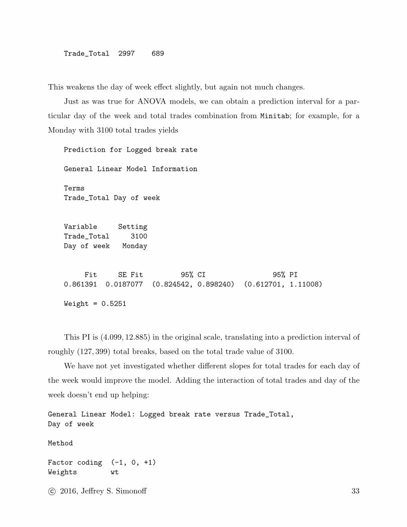
Trade_Total 2997 689
This weakens the day of week effect slightly, but again not much changes.
Just as was true for ANOVA models, we can obtain a prediction interval for a par-
ticular day of the week and total trades combination from Minitab; for example, for a
Monday with 3100 total trades yields
Prediction for Logged break rate
General Linear Model Information
Terms
Trade_Total Day of week
Variable Setting
Trade_Total 3100
Day of week Monday
Fit SE Fit 95% CI 95% PI
0.861391 0.0187077 (0.824542, 0.898240) (0.612701, 1.11008)
Weight = 0.5251
This PI is (4.099, 12.885) in the original scale, translating into a prediction interval of
roughly (127, 399) total breaks, based on the total trade value of 3100.
We have not yet investigated whether different slopes for total trades for each day of
the week would improve the model. Adding the interaction of total trades and day of the
week doesn’t end up helping:
General Linear Model: Logged break rate versus Trade_Total,
Day of week
Method
Factor coding (-1, 0, +1)
Weights wt
c© 2016, Jeffrey S. Simonoff 33

Factor Information
Factor Type Levels Values
Day of week Fixed 5 Friday, Monday, Thursday, Tuesday,
Wednesday
Analysis of Variance
Source DF Adj SS Adj MS F-Value P-Value
Trade_Total 1 0.64276 0.642761 78.13 0.000
Day of week 4 0.01003 0.002508 0.30 0.875
Trade_Total*Day of week 4 0.02318 0.005796 0.70 0.590
Error 240 1.97433 0.008226
Lack-of-Fit 236 1.95552 0.008286 1.76 0.314
Pure Error 4 0.01881 0.004703
Total 249 3.40282
Model Summary
S R-sq R-sq(adj) R-sq(pred)
0.0906993 41.98% 39.80% 36.72%
Coefficients
Term Coef SE Coef T-Value P-Value VIF
Constant 1.1006 0.0288 38.21 0.000
Trade_Total -0.000083 0.000009 -8.84 0.000 1.67
Day of week
Friday -0.0117 0.0766 -0.15 0.879 94.80
Monday -0.0587 0.0674 -0.87 0.385 59.48
Thursday 0.0253 0.0525 0.48 0.630 49.89
Tuesday 0.0112 0.0403 0.28 0.781 37.89
Trade_Total*Day of week
Friday 0.000003 0.000025 0.13 0.894 95.13
Monday 0.000028 0.000023 1.23 0.219 64.21
Thursday -0.000001 0.000017 -0.06 0.956 50.01
Tuesday -0.000013 0.000013 -0.99 0.323 38.38
c© 2016, Jeffrey S. Simonoff 34

Regression Equation
Day of week
Monday Logged break rate = 1.0419 -0.000055Trade_Total
Tuesday Logged break rate = 1.1118 -0.000096Trade_Total
Wednesday Logged break rate = 1.1344 -0.000101Trade_Total
Thursday Logged break rate = 1.1259 -0.000084Trade_Total
Friday Logged break rate = 1.0889 -0.000080Trade_Total
If this were the model of choice, there would be different slope terms for each day of the
week, as can be seen in the output. The t–test for each interaction coefficient refers to
whether the coefficient for that level of the grouping variable is significantly different from
the overall coefficient for all groups (the overall coefficient is just the average of the slopes
for all of the groups, and its estimate is given in the output as −0.000083). The missing
coefficient corresponds to the last group that appears in the data. Since effect codings are
used, the coefficients must sum to zero, so it equals the sum of the other groups’ coefficients
multiplied by −1.
The model that includes the interaction effect between the day of the week and the
total number of trades corresponds to separate regression lines for each day of the week.
Since we only have one numerical variable, we can actually represent that graphically with
separate lines on the same plot:
c© 2016, Jeffrey S. Simonoff 35

It is not surprising from these plots that a model with different slopes is not significantly
better than a model with the same slope, although there is a suggestion that Monday might
be different from the other days. Note that an ANOVA interaction plot is not appropriate
in this context of trying to represent a different slopes effect.
So, what have we learned? Most importantly, perhaps, there are real differences in
break rate based on the day of the week. These differences seem important, as they
represent 10–20% differences in break rate between the middle of the week and the ends
of the week. Since trades come in on all days, further investigation of how to improve
c© 2016, Jeffrey S. Simonoff 36

performance on Mondays, Thursdays and Fridays seems warranted.
Minitab commands
By default, side–by–side boxplots are given with the boxes ordered either numerically
or alphabetically, as appropriate. This is fine if the categories are defined numerically, but
might not be if they are identified by text. If the default plot doesn’t put the boxes in the
right order, create a variable that defines them numerically, with the numbers assigned
corresponding to the appropriate ordering of the categories (this is done by clicking on
Data → Code → Text to Numeric). Create the side-by-side boxplots in the usual way,
based on the numerical grouping variable just created. Double click on any of the numeric
values that labels for the boxes (below the horizontal axis). Click on the Labels tab and
then the radio button next to Specified, and replace the numeric values in the dialog box
with the text labels given in the correct order.
An analysis of covariance is conducted by clicking on Stat → ANOVA → General Lin-
ear Model → Fit General Linear Model. Enter the target variable under Responses:,
the categorical predictor(s) under Factors:, and the numerical predictor(s) under Co-
variates:. Fitted means, residual plots and storage are obtained as stated earlier in the
ANOVA-related handouts.
Multiple comparisons for categorical predictor(s) in a constant shift ANCOVA model
are obtained in the same ways as are discussed for ANOVA models in the handouts related
to those models.
A Levene’s test when fitting an ANCOVA model can be defined based on both the
categorical and numerical variable(s) using ANCOVA fit to the absolute residuals, although
in that case you probably don’t need to include an interaction effect in the model (note that
this was not done in this handout, where heteroscedasticity was only modeled as a function
of the categorical predictor, day of week). A weighted analysis is obtained by entering a
weight variable under Options. Note that if the observed heteroscedasticity appears to
be related to the numerical variable in the Levene’s test ANCOVA model (as well as the
categorical variable, perhaps), weights should be obtained by saving the residuals from
c© 2016, Jeffrey S. Simonoff 37

the original ANCOVA fit, forming the log(residuals2) variable, constructing an ANCOVA
fit with that variable as the target, saving the fitted values from that fit, and setting the
weight variable to 1/exp(FITS). See the “CAPM: Do you want fries with that?” handout
for an example of this.
To fit a model with different slopes for each group, add the interaction effect of the
categorizing variable(s) with the covariate(s) using the same method as was done in two-
way ANOVA. Minitab uses effect codings to fit the models, and as a result estimated slopes
and t-statistics will only be presented for K−1 of the groups, with the coefficient for the last
group (alphabetically) being left out (recall that these coefficients correspond to deviations
from the overall coefficient given earlier in the output). The estimated coefficient for the
omitted group is simply the negative of the sum of the other coefficients (since they must
sum to zero), but if you want to obtain a t-statistic for that slope you must rename the
group so that it is no longer the last one alphabetically.
Remember, an interaction plot is not appropriate for interactions involving covariates;
a scatter plot with different regression lines superimposed is. To construct such a plot,
click on Scatterplots and then With Regression and Groups. Enter the target variable
under Y variables, the predictor under X variables, and the variable that defines the
groups under Categorical variables for grouping. To delete the data points from
the plot (leaving only the regression lines), right click on the plot, then click Select →
Symbols, and press the Delete key.
c© 2016, Jeffrey S. Simonoff 38