analysis of ema systems in mea applications8177/fulltext01.pdf · fault tolerant electrical power...
TRANSCRIPT

TRITA-ETS-2005-10 ISSN 1650-674x
ISRN KTH/R-0504-SE ISBN 91-7178-099-8
May, 2005
Analysis of Electro-Mechanical Actuator Systems in More Electric
Aircraft Applications
Mohsen Torabzadeh-Tari
DEPARTMENT OF ELECTRICAL ENGINEERING
ROYAL INSTITUTE OF TECHNOLOGY SWEDEN

Submitted to the School of Computer Science, Electrical Engineering and Engineering Physics, KTH,
in partial fulfilment of the requirements for the degree of Licentiate of Technology.
Stockholm 2005
TRITA-ETS-2005-10 ISSN-1650-674x
ISRN KTH/R-0504-SE ISBN 91-7178-099-8
© Mohsen Torabzadeh-Tari, Stockholm, 2005

To my love Zohreh


Abstract
Abstract
Conventional hydraulic actuators in aircraft are demanding regarding maintenance which implies high operation costs. In recent years the focus therefore has been set on electro-hydrostatic and electro-mechanical actuators.
The aim of this work is to analyze and evaluate the possibility of introducing electro-mechanical actuators (EMAs) in more electric aircraft applications. The major goal is to optimize the weight of such actuator systems including the electro-machine (electric motor) gear mechanism and power converter, without loss of reliability. Other optimisation criteria on such solutions are low losses and good thermal properties.
A quasi-static model approach of EMAs is used here in order to decrease the simulation time. It is possible because the low (mechanical) and high (electrical) frequency components are separated in the model, see [1]. The inverters and converters are described as fictive DC-DC transformers with corresponding efficiencies, see [2]. By introducing an object oriented approach the model is flexible and re-usable and can be used as a framework in the future build-up of models of entire MEA aircrafts, see [3].
Power density, cost and weight of the actuator systems are some of the important key factors for comparing purpose and as a platform for the dimensioning of the aircraft. The next issue becomes the scalability of the model and the key factors, because of the diversity of the actuators used in different parts of the MEA aircraft. Therefore the ambition is set to build up a database of different scalable actuator solutions which among others returns these key factors as output.
I
Abstract
Keywords
• MEA • More Electric Aircraft • EMA • Electro Mechanical Actuator • EM • Electrical Machine • Converter • Inverter • EHA • Electro Hydrostatic Actuator • Power-by-Wire • Finite Element Method • FEM • Object Oriented • Modelica
II
Acknowledgement
Acknowledgement
I would like to express a general gratitude to the people who have helped me in various ways with this research and a making pleasant atmosphere in the department.
Special thanks to Prof Göran Engdahl, for his guidance and sharing of his experience during these years. The discussions with him are always inspiring and fruitful. There are numerous notebooks in my bookcase containing discussions note from our informal meetings, used often as reference in this thesis.
I would also like to thanks the head of department Prof Roland Eriksson for offering me this position and making a light atmosphere in the department to work in. Mr. Peter Lönn, and Mr. Göte Berg are two other wonderful persons who have a major part of the ordinary day-to-day work. Their helpfulness is appreciated. The ‘administrative’ help from Mr Olle Brännwall, Mr. Jan Timmerman, and Mrs Eva Peterson, Mrs Astrid Myhrman, and Mrs Margareta Surjadi is also highly appreciated.
Many thanks to Mr. Lars Austrin who has shared his experience and study time with me during these years. His generosity is highly appreciated, specially during the numerous discussions at our home trip towards Linköping.
Thanks also to Dr Peter Thelin, Dr Freddy Magnusson, Tech. Licentiate Maddalena Cirani, Prof Hans Peter Nee, Tech. Licentiate Mats Leksell, Dr Karsten Kretschmar, Dr Erik Nordlund, Dr Hans Edin, and Dr Niclas Schönborg for their patience and helpfulness when explaining the underlying physical laws and mechanism of the rotary machines. Dr Julius Krah, whom I share my office with, should also be mentioned. Thanks for putting up with my radio listening during these years. Also Mr. Nathaniel Taylor is appreciated for his assistance in Linux.
III

Acknowledgement
I would also like to express my gratitude to people behind the NFFP-discussion group, Dr Björn Johansson, Prof Petter Krus, Mr. Jan-Erik Nowacki, Dr Jonas Larsson, Mr. Anders Järlestål, and Mr. Hans Ellström for their insightful discussions.
A special gratitude to Mr. Björn Hellström at ABB Research Center for his assistance of the FEM program Ace and Mr. Lennart Stridsberg for providing information about his innovative machine.
Finally I would like to thanks my wife for her endurance during these last three years. Thanks for staying up until late and helping me with the numerous FEM simulations. Without your contribution I would have been forced to simplify the problem to verification of Ohm’s law. My parents, sisters, brother, and the rest of the ‘BIG2’ family and relatives for their support during all the years. Without your endless support and believe in me, I would not have reached this fare. You are always in my heart, thought and prayers.
Mr. Janne ‘T’ Andersson, Mr. K-G Alhström, Mrs. Guje Alhström, Mr. Abdullah Rajabi, Mrs. Eva Åberg and late Mr. Åke Åberg have always a special place in my heart.
To the rest whom I have not mentioned, you are not forgotten and always in my heart.
At last but not least people at FMV and Vinnova and Mr Lars Austrin from Saab AB who once started this project and financed my research should be mentioned and thanked. The funding and prolonging of this project is indebt to the efforts of Mr Lars Austrin and highly appreciated.
Stockholm, May 2005
Mohsen Torabzadeh-Tari
IV

Contents
Contents
CHAPTER 1 INTRODUCTION................................................................... 1
1.1 BACKGROUND ........................................................................................ 1 1.2 AIM ........................................................................................................ 4 1.3 OUTLINE OF THE THESIS ......................................................................... 5 1.4 LIST OF PUBLICATIONS ........................................................................... 5
CHAPTER 2 PROBLEM INTRODUCTION ............................................. 7
2.1 CHARACTERISTICS OF ACTUATORS IN AIRCRAFT APPLICATION ............. 7 2.2 DESIGN PARAMETERS............................................................................. 9
CHAPTER 3 THE ELECTRO-MECHANICAL ACTUATOR .............. 13
3.1 COMPONENTS OF AN ELECTRO-MECHANICAL ACTUATOR.................... 13 3.2 THE ELECTRICAL-MACHINE................................................................. 13
3.2.1 DC Electrical Machines .................................................................. 15 3.2.2 Induction Electrical Machines ........................................................ 16 3.2.3 Reluctance Electrical Machines...................................................... 16 3.2.4 Permanent Magnet Electrical Machines......................................... 18
3.3 THE ELECTRONIC POWER CONTROL..................................................... 23 3.4 THE GEAR ............................................................................................ 26 3.5 THE COMPLETE ACTUATOR.................................................................. 27
CHAPTER 4 METHODS ............................................................................ 29
4.1 ANALYSIS TOOLS ................................................................................. 29 4.2 MODELLING AND ANALYSIS................................................................. 29
4.2.1 Loss Models..................................................................................... 32 4.2.2 Modeling of the Permanent Magnet................................................ 43
4.3 OPTIMIZATION OF THE EMA ................................................................ 45
CHAPTER 5 RESULTS............................................................................... 47
5.1 INTRODUCTION..................................................................................... 47 5.2 2D FEM ANALYSIS OF THE ELECTRICAL MACHINE .............................. 47
5.2.1 Losses .............................................................................................. 64 5.3 SIMPLIFIED EQUIVALENT CIRCUIT SIMULATION................................... 74
5.3.1 Flight Mission Simulations ............................................................. 75
V

Contents
CHAPTER 6 THERMAL ANALYSIS....................................................... 85
6.1 ANALYSIS TOOLS ................................................................................. 85
CHAPTER 7 OTHER SOLUTIONS.......................................................... 89
7.1 CONVENTIONAL HYDRAULIC ACTUATORS ........................................... 89 7.2 MAGNETOSTRICTIVE ACTUATORS........................................................ 90 7.3 ELECTRO-HYDROSTATIC ACTUATOR ................................................... 92
CHAPTER 8 CONCLUSIONS AND FUTURE WORK .......................... 95
8.1 CONCLUSIONS ...................................................................................... 95 8.2 FUTURE WORK ..................................................................................... 96
APPENDIX A .................................................................................................... 99
APPENDIX B................................................................................................... 101
REFERENCES ................................................................................................ 103
LIST OF SYMBOLS....................................................................................... 109
INDEX .............................................................................................................. 115
VI
Introduction Chapter 1
Chapter 1 Introduction
1.1 Background
There is a general trend in aerospace industry to increase the use of electrically powered equipment. This trend is usually referred to as “More Electric Aircraft” (MEA) or “Power-by-Wire”. The benefits are among others lower maintenance effort, higher efficiency and larger fault tolerance. In fact this idea is not new, the Vickers Valliant used a 112 VDC electrical system together with electrical flight control during the World War II. However the required power for such electric systems exceeded the generated power and therefore this approach was unfeasible until recently. Advances in enabling technologies of electric power generation, distribution and consumption have made “Power-By-Wire” more competitive than before, see [4]-[8]. The benefits, such as no rotor winding losses of switched reluctance machine and good efficiency and good cooling capability of permanent magnet generators are discussed in [9]-[11] for MEA applications.
In Figure 1.1 a block scheme of the power system of a MEA is shown. The power is transported in ‘wires’ between the devices. In Figure 1.2 a MEA is shown, with electric anti-ice system for flight control critical surfaces, electric actuators, and electric brakes.
1

Chapter 1 Introduction
Figure 1.1 Block scheme of a MEA power system concept.
Battery
APU Generator
Landing Gear, Brake
Electric Anti-Ice
Electronic Power Controllers
Battery
Fault Tolerant Electrical Power Managment and Distribution System
Electric Engine
Electric Drive Accessories Environment Control Electric Drive
Flight Control
Figure 1.2 The More Electric Aircraft.
2

Introduction Chapter 1
The MEA concept also includes new high power, electric actuation systems for moving the flight control surfaces such as rudder, aileron, spoiler etc. for controlling the speed and direction of the aircraft during the flight. Such actuators are either Electro-Hydrostatic, EHA or Electro-Mechanical, EMA. In the EHA solution a distributed hydraulic system is used while in the EMA the hydraulics is replaced by an Electrical-Machine, gearbox and/or a screw mechanism, see [8].
Figure 1.3 An Advanced Motor Derive (AMD) EMA.
In Figure 1.3 an EMA from Propulsion Directorate and Hamilton Sundstrand is shown, with an electric motor, screw and gear mechanism, see also [12]. For this EMA the efficiency for electric to mechanic power conversions greater than 81%, and a life-cycle cost reduction by at least 10% is promised
Conventional hydraulic actuators of today are quite heavy, maintenance demanding and more vulnerable to high temperature and pressure because of their flammable liquids compared to the MEA actuators. However, the dynamic nature of the loads of such actuators requires a controllable power supply. Another benefit of the EMA is the ability of regenerating the power from the actuator, instead of heating up resistors.
There are also spin-off effects from the MEA technology that are worth mentioning. For example the electric brake, see Figure 1.4, produced for the aircraft manufacturer Boeing.
3

Chapter 1 Introduction
Figure 1.4 The electric brake, containing an electric motor, gear, ball screw, rotor and stator discs.
In Figure 1.4 an electric actuator system is replacing the traditional hydraulic piston system: it is made up of an electric motor (1), a ball screw (2 and 3) and a speed reducer (4 and 5), see also [9].
1.2 Aim
The major goal of this thesis is to contribute to the knowledge on electro mechanical actuators for more electric aircraft applications. This analysis can be performed by building up a data base of key technical parameters, like power density, cost, and average efficiency of these actuators in an aircraft power system context. For this reason a simplified quasi-static actuator model has been developed. This model makes it possible to reduce the complexity of the actuator models to such extent that the resulting computional tool can be used for studies of the system performance during entire flight missions and/or for optimisation. The ambition is then to build up a database of different actuator solutions with the key technical parameters mentioned above, that can be used in modelling and dimensioning of aircraft.
4

Introduction Chapter 1
1.3 Outline of the Thesis
Chapter 2 gives a description of the behaviour of the MEA actuator loads. The dynamic nature of those is then translated into requirements and design parameters.
Chapter 3 gives a basic insight of the components of an EMA. Basic equations and fundamentals are presented during normal and transient operations.
Chapter 4 gives a description of the object oriented language Modelica, the simulation environment Dymola and the FEM-software Ace. A quasi-static model of the more electric aircraft electromechanical actuator is developed, introduced in articles [1] and [2] with co-writers Prof Engdahl, and Mr Lars Austrin described in chapter 4.
Chapter 5 gives a summary and analysis of the performed simulations. The parameters like back-EMF and torque constant have been retrieved from FEM analysis. These parameters were used in the quasi-static actuator model to relate the mechanical side of the actuator to the electrical side. The level of the DC-bus voltage, losses and power levels were studied.
Chapter 6 gives a brief insight of the thermal situation of the EM that has been analysed. The iron, copper and magnet losses are calculated and used in a FEM analysis for studies of the winding and magnet temperatures.
Chapter 7 gives a brief comparison between the EHA, the conventional hydraulic and the new EMA solutions.
Chapter 8 summarises the work, draws conclusions and gives suggestions for future work. A database of different technologies can be build up for a better and more complete comparison. The thermal analysis can be build in the quasi-static model of the power system itself, see also [22].
1.4 List of publications
Some of the results in this thesis have been published in the publications below.
5

Chapter 1 Introduction
• M. Torabzadeh-Tari and G. Engdahl: “A Quasi-Static Modelling Approach of Electromechanical Actuators”. The Proceedings of the 2003 International Conference of Magnetism - ICM 2003, Rome, Italy, July 27-1 August, 2003.
• M. Torabzadeh-Tari, G. Engdahl, L. Austrin and J. Krah: “A Quasi-Static Modelling Approach Airborne Power Systems”. The 11th National Conference on Machine and Mechanics – NaCoMM 2003, New Dehli, India, December 18-19 2003.
• M. Torabzadeh-Tari, G. Engdahl: “A Portable Implementation of a Model of Electromechanical Actuators in More Electric Aircraft Dimensioning Tools”. Actuator 2004, Bremen, Germany, June 14-16 2004.
6
Problem Introduction Chapter 2
7
Chapter 2 Problem Introduction
2.1 Characteristics of Actuators in Aircraft Application
Conventional hydraulic actuators are centralized which require a high amount of pipes for the actuator liquid. This implies a high vulnerability and maintenance level. The new technology referred to as MEA actuators, which uses either a localized hydraulic solution, EHA or an electro-mechanical actuator does not show the same vulnerability as a conventional hydraulic system, regarding the flammable oil and maintenance of the pipe system. There is also a third MEA actuator type, the magnetostrictive type which is mentioned in chapter 7.2. In addition to the higher efficiency, lower cost and weight offered by the MEA solutions there is also a possibility to re-generate energy from the motion of the actuators back to the power system.
The motion of the control surfaces of a MEA shows a dynamic nature. On top of the dynamic behaviour these movements are often applied under very short periods of time, “dirac-like” behaviour, which require quite high torque output of the actuator. Therefore a high power density of the equipment is favourable. A simplified motion profile of an Unmanned Airborne Vehicle, UAV actuator is given in Table 2.1.

Chapter 2 Problem Introduction
8
Table 2.1 An example of an UAV mission profile.
Mode Engine start
Test/ Taxiing
Take off
Cruise Mission Landing
Duration [min]
1 5 3 30 18 3
Actuator angular speed [rad/s]
- [-1,1] [-2,2] [-0.1,0.1] [- 0.5,0.5] [-1,1]
Torque [Nm]
- 5 800 200 800 200
Frequecy [Hz]
- 0.5 0.2 2 0.3 2
From Table 2.1 the instantaneous maximum power is 800 0.3 2 800 1.89π⋅ ⋅ ⋅ = ⋅ =1.5 [kW] that the actuator must deliver. Assuming a screw mechanism with the conversion rate 300, yielding that the electrical
machine must be able to operate at 1.89*300=567 rads
⎡ ⎤⎢ ⎥⎣ ⎦
and deliver 800300
=2.8
[Nm]. During a flight mission the actuators consume, in average, a power that is quite lower than the maximum required power, 1.5 [kW]. The low average power consumption comes from the fact that aircraft actuators have frequent starts and stops during its operation. If the average power level is set as an optimized working point, then for passing the maximum power requirement the operating range must be widened. The widened operation range means in its turn tougher requirements on the machines involved. This can be a source of conflict. The conflict is naturally to compromise between finding an optimized working point and to be able to deliver a higher instantaneous maximum power.
Another characteristic of an aircraft actuator is the exposure to different environmental and atmospheric conditions. Altitude, temperature and humidity of air are examples of such important environment parameters that influence (i.e. restrict) the operation of the actuator. Flying at lower altitude and following the ground curvatures means high power (i.e. torque) consumption, while flying at high altitude without changing the flight route means a lower power requirement. Higher temperature will for example increase the copper losses which means higher power consumption. It is a well known fact that fluids, like

Problem Introduction Chapter 2
9
water, can cause short circuits in electrical circuits. Therefore the humidity of air should be kept out from the electric machine of the actuator.
2.2 Design Parameters
The parameters used for comparison of different actuator solutions can be divided in two kinds, a low and a high level. The low level parameters come from the requirement of functionality of the device, and the high level parameters come from a system perspective. For example an electro machine
must deliver 10 [kNm] at an angular frequency of 1 rads
⎡ ⎤⎢ ⎥⎣ ⎦
, at the functional
level. At the system level it should for example cost below 300 [kSEK].
Features like reliability, average power consumption, and cost are examples of factors that are of interest at system level.
The cooling capability of the device for a given output torque is an example of a functional parameter that should be considered. The reason is the obvious lack of space and cooling power in an aircraft. Other important functional parameters in evaluation of an electrical machine are among others inductance, magnetic flux, field weakening range, and saliency level. Regarding the power electronics the harmonic level (i.e. harmonics created from the switches) of the electrical power delivered to the electrical machines are crucial. These harmonics will cause additional losses. The non-jamming capability of the screw mechanism is also important functional issue that must be studied.
In an aircraft application, operation redundancy is a quite well known requirement in critical flying systems. The actuators are no exception of this. The operation of an actuator can for example be redundant either by dividing the rudder area in smaller parts connecting an actuator to each part or coupling two actuators in parallel working on the same rudder surface. In the passenger carrier A380 from the aircraft manufacturer Airbus rudder surface control is done by three redundant connected actuator pairs in parallel. The third redundant actuation system is an EHA solution.

Chapter 2 Problem Introduction
10
The environmental requirements mentioned in previous section will naturally influence the design. Actuators can for example be build with drain holes for avoiding moisture problems.
A dirac-like torque requirement will cause current harmonics delivered from the inverter electronics that must be compensated by capacitive filters. Current harmonics will increase the eddy current losses in the core and permanent magnets. This is why the harmonic content of the supply current is undesired and must be filtered out. This implies an increase of the number of electronic components and increased weight.
An unspoken requirement on aircraft apparatus is about the power supply. In order to avoid a situation with several power lines at different voltage levels, each apparatus should contain a converter that is adapted for a single voltage level. This requirement can increase the size of the of the power supply.
The re-generation ability of an electro mechanical actuator can be a disadvantage from safety perspective. Therefore often a resistor bridge is used for heating up the fed back power instead of letting it go back to the power system. Therefore a ‘resistor bridge’ can be needed.
Designing a fault tolerant and flight worthy EMA is the basic requirement of a MEA EMA. An example of such a functional specification, for controlling a 40 [kW] spoiler surface, is given in Table 2.2, see also [15].
Problem Introduction Chapter 2
11
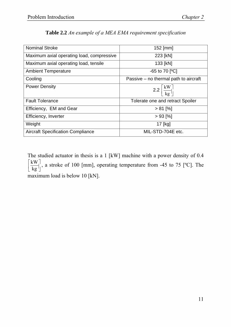
Table 2.2 An example of a MEA EMA requirement specification
Nominal Stroke 152 [mm] Maximum axial operating load, compressive 223 [kN] Maximum axial operating load, tensile 133 [kN] Ambient Temperature -65 to 70 [ºC] Cooling Passive – no thermal path to aircraft Power Density
2.2 kWkg
⎡ ⎤⎢ ⎥⎣ ⎦
Fault Tolerance Tolerate one and retract Spoiler Efficiency, EM and Gear > 81 [%] Efficiency, Inverter > 93 [%] Weight 17 [kg] Aircraft Specification Compliance MIL-STD-704E etc.
The studied actuator in thesis is a 1 [kW] machine with a power density of 0.4 kWkg
⎡⎢⎣ ⎦
⎤⎥ , a stroke of 100 [mm], operating temperature from -45 to 75 [ºC]. The
maximum load is below 10 [kN].


The Electro-Mechanical Actuator Chapter 3
13
Chapter 3 The Electro-Mechanical
Actuator
3.1 Components of an Electro-Mechanical Actuator
An EMA could be divided into three main parts, an inverter, an electrical-machine and finally a gear-mechanism. This gives the opportunity to combine different types of the components to find an optimal combination.
3.2 The Electrical-Machine
An electrical machine (EM) can handle power conversion in both directions, electrical to mechanical (motor) and mechanical to electrical (generator).
There are several different electrical machine types, presented in [16] suitable for EMA applications. A rough comparison between these electrical machines is presented in Table 3.1.

Chapter 3 The Electro-Mechanical Actuator
14
Table 3.1 Comparison between electrical machines, AM, PMSM, SR and SM
AM PMSM SR SM Power density 1 2 3 4 Maintenance need 1 1 1 2 Reliability 1 3 2 4
From Table 3.1 one can see that the Synchronous Machine (SM) has the highest power density and reliability. The other electrical machines in Table 3.1, Asynchronous Machine (AM), Permanent Magnet Synchronous Machine (PMSM) and the Switched Reluctance (SR) machine have lower power densities and reliability than the SM. All four electrical machines have almost the same maintenance requirement.
In a synchronous electrical machine the rotor position is required for the ability to control the currents sinusoidally and synchronous with the rotor. Only currents synchronous with the rotor contribute to the torque production. Other characteristics of synchronous electrical machines are low torque ripple, good low speed and positioning behaviour, and low harmonic losses. The DC machine needs a simpler position sensor and usually has higher torque ripple.
Temperature is often mentioned as a critical dimensioning parameter. The losses related to the windings of the electrical machines will increase with temperature (i.e. copper resistance is temperature dependent). In electrical machines with permanent magnets the coercive and remanence force of the permanent magnets decrease with increasing temperature. The temperature also has a demagnetizing effect on the permanent magnets.
Another disadvantage related to the electrical machines with permanent magnets is the constant coercive force that cannot be turned off in critical situations. In these situations a high reactance in the stator tooth is favourable. Phase short-circuits is one example of such critical operation modes that can occur in an electrical machine. In combination with the constant flux from the permanent magnets a breakdown of the machine then can occur.
The Electro-Mechanical Actuator Chapter 3
15
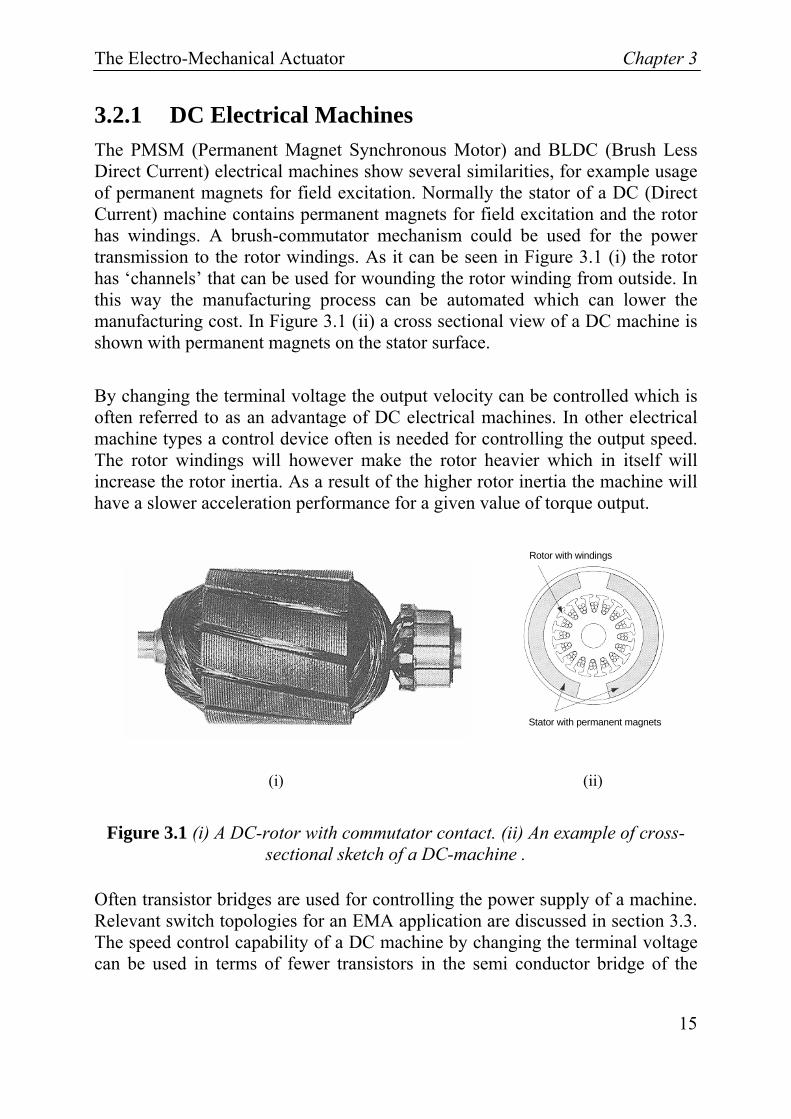
3.2.1 DC Electrical Machines The PMSM (Permanent Magnet Synchronous Motor) and BLDC (Brush Less Direct Current) electrical machines show several similarities, for example usage of permanent magnets for field excitation. Normally the stator of a DC (Direct Current) machine contains permanent magnets for field excitation and the rotor has windings. A brush-commutator mechanism could be used for the power transmission to the rotor windings. As it can be seen in Figure 3.1 (i) the rotor has ‘channels’ that can be used for wounding the rotor winding from outside. In this way the manufacturing process can be automated which can lower the manufacturing cost. In Figure 3.1 (ii) a cross sectional view of a DC machine is shown with permanent magnets on the stator surface.
By changing the terminal voltage the output velocity can be controlled which is often referred to as an advantage of DC electrical machines. In other electrical machine types a control device often is needed for controlling the output speed. The rotor windings will however make the rotor heavier which in itself will increase the rotor inertia. As a result of the higher rotor inertia the machine will have a slower acceleration performance for a given value of torque output.
Rotor with windings
Stator with permanent magnets (i) (ii)
Figure 3.1 (i) A DC-rotor with commutator contact. (ii) An example of cross-sectional sketch of a DC-machine .
Often transistor bridges are used for controlling the power supply of a machine. Relevant switch topologies for an EMA application are discussed in section 3.3. The speed control capability of a DC machine by changing the terminal voltage can be used in terms of fewer transistors in the semi conductor bridge of the

Chapter 3 The Electro-Mechanical Actuator
16
feeding inverter. A DC machine drive needs at least four transistors against the six in an ordinary H-bridge for a traditional three phase machine.
3.2.2 Induction Electrical Machines Induction or asynchronous electrical machines can be used without inverter or control electronics and therefore are very popular in the industry. Robustness and low cost are also other advantages that often are mentioned regarding induction electrical machines. In electric vehicles, induction machines can be supplied with a variable speed control accomplished by a frequency inverter.
(i) (ii)
Figure 3.2 (i) X-ray image of a squirrel-cage induction machine (ABB). (ii) Cross-sectional drawing of a quarter of a four-pole induction machine.
Short-circuited aluminium bars, a squirrel cage, are often used instead of rotor windings, see Figure 3.2 (i). The current in the rotor bars has an unpleasant side-effect, temperature rise. It is difficult to cool the rotor and therefore as a consequence the lifetime of the machine or the output power may be decreased. A four pole induction machine cross sectional view is shown in Figure 3.2 (ii).
3.2.3 Reluctance Electrical Machines There are two types of reluctance electrical machines, synchronous and switched reluctance machines, see Figures 3.3 and 3.4. Both show similarities with the induction machine with respect to the stator design.

The Electro-Mechanical Actuator Chapter 3
17
The rotor of a synchronous reluctance machine can be manufactured with punched iron laminations which could lead to cost savings in the manufacturing process.
Often the vector representation of the electrical quantities of a three phase machine is transformed by Park transformation to d-q quantities. The d-q coordinate system has the rotor as origin and rotates with rotor. The ‘d’ stands for direct current direction, ‘q’ for quadrature and is orthogonal to the d-axis. In a synchronous reluctance electrical machine the structure with air in the iron on the rotor, “air channels in the iron”, increases the d-inductance, see Figure 3.3. This will maximize the torque output of the machine. However the synchronous reluctance machine has poor damping which can result in a rough start performance. At starts the poor damping of the electrical machine will cause ‘inrush currents’ into the stator phases, which will produce a high initial torque output. Controlling the motion of a MEA actuator is crucial during the flight missions. Further is the starting characteristic of a MEA actuator critical since its operation comprises frequent starts and stops. Therefore a ‘soft’ starting behaviour is to prefer. The synchronous machine is not considered for further analysis in this project due to its rough starting performance.
Air pockets
Iron bridges
Stator
Rotor
Figure 3.3.Cross-sectional sketch of a synchronous reluctance machine.
In a switched reluctance machine both the rotor and the stator have salient poles. In this machine the torque is generated by the stator current excitation and the fact that the rotor tends to move to minimize the reluctance. In Figure 3.4 several reluctance machines are shown, with different phase and pole numbers.

Chapter 3 The Electro-Mechanical Actuator
18
(i) (ii) (iii) (iv) (v) (vi)
Figure 3.4 Several types of reluctance machines. (i) 4-pole 3-phase, (ii) 6-pole 4-phase, (iii) 8-pole 5-phase machine, (iv) full-pitch 4-pole 3-phase, (v) stepped-
gap 2-pole 2-phase and (vi) 10-pole 3-phase machine.
The control of the movement is achieved by switching the appropriate phase current. Robustness and cost effectiveness are two advantages of such a design beside its low rotor losses. The machine has a “digital” movement behaviour which causes a high torque ripple output.
Angle Θ ( mec. deg.)
τ [Nm]
Figure 3.5 An example of a torque variation in a reluctance electrical machine.
An example of the torque ripple is shown in Figure 3.5, where the torque is changed in small steps.
3.2.4 Permanent Magnet Electrical Machines The direction of the active air gap flux density is often used for dividing PM electrical machines in sub-categories, namely radial, axial and transversal PM machines.

The Electro-Mechanical Actuator Chapter 3
19
Most common PM electrical machine is the radial flux machine. The popularity can be explained by the capability of increasing torque and power of the machine simply by stacking more laminated iron in the axial direction. In such machines the rotor is often placed inside the stator core. The mounting of the magnet will in its turn divide these machines in three sub-categories, namely surface-mounted, inset and interior rotor designs. In Figures 3.6-3.9 the principal sketch of these three machine type are shown.
magnetd
q
Iron
Figure 3.6 Basic cross-section of a two pole rotor with surface mounted magnets and its d-q coordinate system.
The surface mounted radial PM electrical machine is shown is Figure 3.6. In high speed applications some form of bandage arrangement could be required to keep the magnets in position. High energy permanent magnets, as NdFeB (Neodymium Iron Boron), have a relative permeability close to 1. The surrounding air has also almost the same relative permeability, yielding a negligible leakage flux. Therefore the reluctance in the flux paths along both q and d axis are the same, yielding low saliency. The magnet surfaces will be also exposed to eddy currents causing additional losses.
The air gap between the magnets on the surface of the rotor could also be replaced by iron in an inset radial PM electrical machine, see Figure 3.7. The reluctance along the d and q-axis are then not equal which results in saliency. More magnet material is required in an inset machine compared to a surface mounted. The reason is the increase of the flux leakage.
Chapter 3 The Electro-Mechanical Actuator
20
magnetd
q
Iron
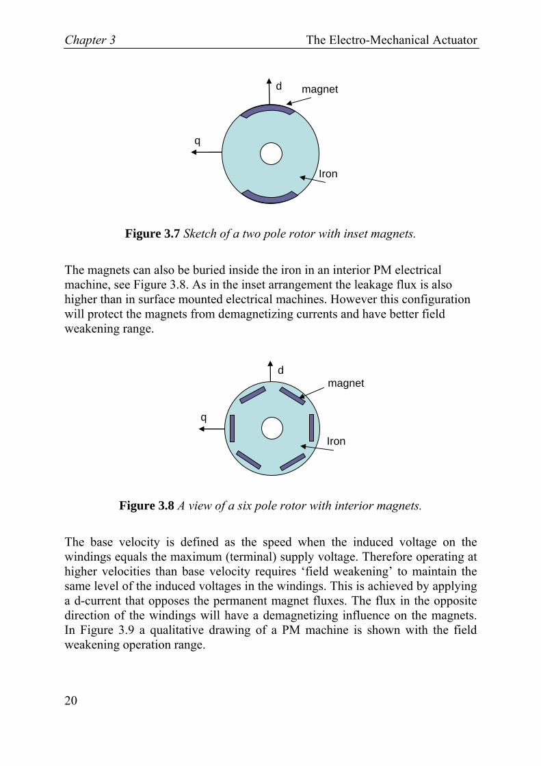
Figure 3.7 Sketch of a two pole rotor with inset magnets.
The magnets can also be buried inside the iron in an interior PM electrical machine, see Figure 3.8. As in the inset arrangement the leakage flux is also higher than in surface mounted electrical machines. However this configuration will protect the magnets from demagnetizing currents and have better field weakening range.
magnet d
q Iron
Figure 3.8 A view of a six pole rotor with interior magnets.
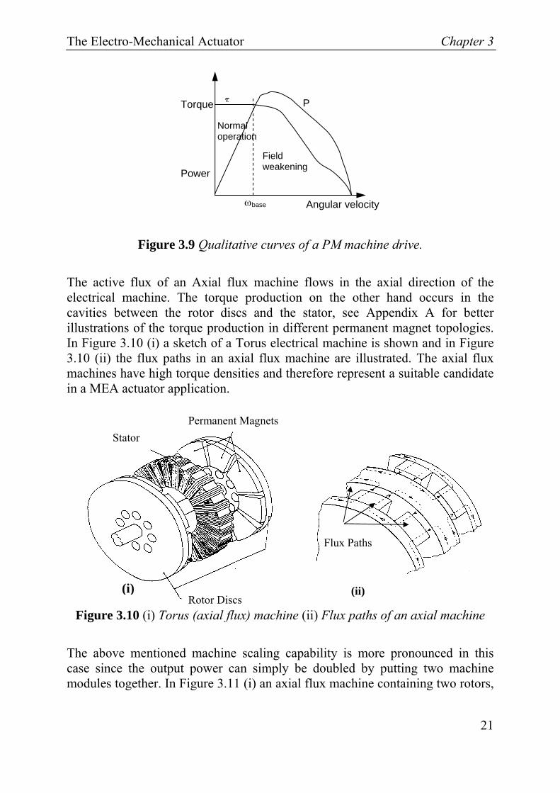
The base velocity is defined as the speed when the induced voltage on the windings equals the maximum (terminal) supply voltage. Therefore operating at higher velocities than base velocity requires ‘field weakening’ to maintain the same level of the induced voltages in the windings. This is achieved by applying a d-current that opposes the permanent magnet fluxes. The flux in the opposite direction of the windings will have a demagnetizing influence on the magnets. In Figure 3.9 a qualitative drawing of a PM machine is shown with the field weakening operation range.
The Electro-Mechanical Actuator Chapter 3
21
Normal operation
Field weakening
P τ
Angular velocity
Torque
Power
ωbase
Figure 3.9 Qualitative curves of a PM machine drive.
The active flux of an Axial flux machine flows in the axial direction of the electrical machine. The torque production on the other hand occurs in the cavities between the rotor discs and the stator, see Appendix A for better illustrations of the torque production in different permanent magnet topologies. In Figure 3.10 (i) a sketch of a Torus electrical machine is shown and in Figure 3.10 (ii) the flux paths in an axial flux machine are illustrated. The axial flux machines have high torque densities and therefore represent a suitable candidate in a MEA actuator application.
Stator
Rotor Discs
Permanent Magnets
Flux Paths
(i) (ii)
Figure 3.10 (i) Torus (axial flux) machine (ii) Flux paths of an axial machine
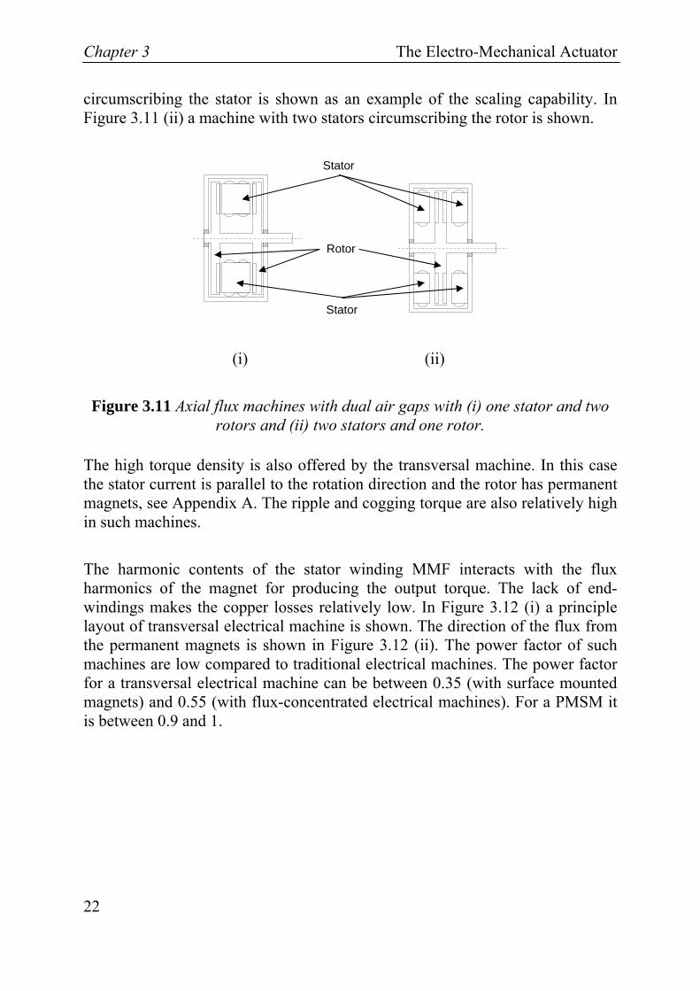
The above mentioned machine scaling capability is more pronounced in this case since the output power can simply be doubled by putting two machine modules together. In Figure 3.11 (i) an axial flux machine containing two rotors,
Chapter 3 The Electro-Mechanical Actuator
22
circumscribing the stator is shown as an example of the scaling capability. In Figure 3.11 (ii) a machine with two stators circumscribing the rotor is shown.
Stator
Rotor
Stator
(i) (ii)
Figure 3.11 Axial flux machines with dual air gaps with (i) one stator and two rotors and (ii) two stators and one rotor.
The high torque density is also offered by the transversal machine. In this case the stator current is parallel to the rotation direction and the rotor has permanent magnets, see Appendix A. The ripple and cogging torque are also relatively high in such machines.
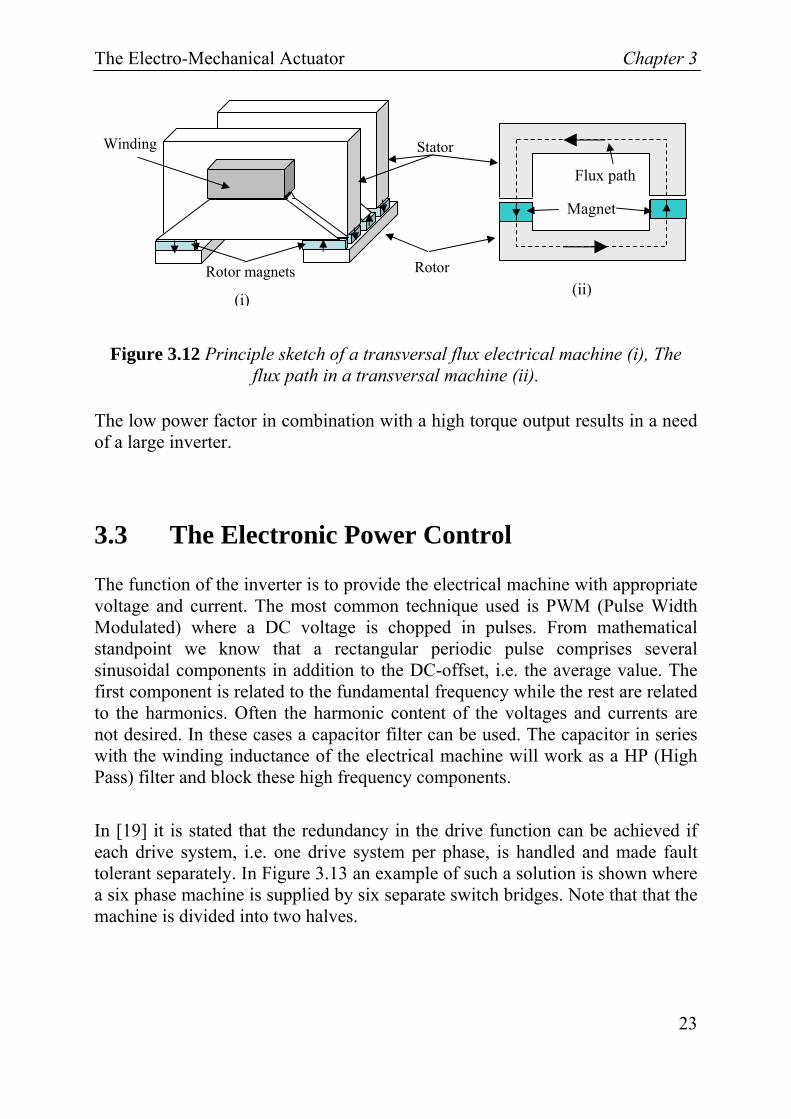
The harmonic contents of the stator winding MMF interacts with the flux harmonics of the magnet for producing the output torque. The lack of end-windings makes the copper losses relatively low. In Figure 3.12 (i) a principle layout of transversal electrical machine is shown. The direction of the flux from the permanent magnets is shown in Figure 3.12 (ii). The power factor of such machines are low compared to traditional electrical machines. The power factor for a transversal electrical machine can be between 0.35 (with surface mounted magnets) and 0.55 (with flux-concentrated electrical machines). For a PMSM it is between 0.9 and 1.
The Electro-Mechanical Actuator Chapter 3
23
Rotor magnets
Stator
Rotor
Winding
Flux path
Magnet
(i) (ii)
Figure 3.12 Principle sketch of a transversal flux electrical machine (i), The flux path in a transversal machine (ii).
The low power factor in combination with a high torque output results in a need of a large inverter.
3.3 The Electronic Power Control
The function of the inverter is to provide the electrical machine with appropriate voltage and current. The most common technique used is PWM (Pulse Width Modulated) where a DC voltage is chopped in pulses. From mathematical standpoint we know that a rectangular periodic pulse comprises several sinusoidal components in addition to the DC-offset, i.e. the average value. The first component is related to the fundamental frequency while the rest are related to the harmonics. Often the harmonic content of the voltages and currents are not desired. In these cases a capacitor filter can be used. The capacitor in series with the winding inductance of the electrical machine will work as a HP (High Pass) filter and block these high frequency components.
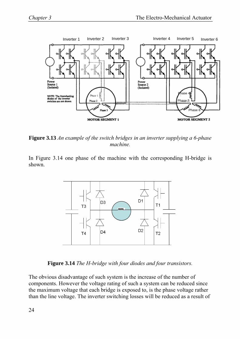
In [19] it is stated that the redundancy in the drive function can be achieved if each drive system, i.e. one drive system per phase, is handled and made fault tolerant separately. In Figure 3.13 an example of such a solution is shown where a six phase machine is supplied by six separate switch bridges. Note that that the machine is divided into two halves.
Chapter 3 The Electro-Mechanical Actuator
24
Inverter 4 Inverter 5 Inverter 6 Inverter 1 Inverter 2 Inverter 3
Phase 4
Phase 5
Phase 6
Figure 3.13 An example of the switch bridges in an inverter supplying a 6-phase machine.
In Figure 3.14 one phase of the machine with the corresponding H-bridge is shown.
Figure 3.14 The H-bridge with four diodes and four transistors.
The obvious disadvantage of such system is the increase of the number of components. However the voltage rating of such a system can be reduced since the maximum voltage that each bridge is exposed to, is the phase voltage rather than the line voltage. The inverter switching losses will be reduced as a result of

The Electro-Mechanical Actuator Chapter 3
25
this, which can be used in form of a reduced heat sink demand, implying weight savings. The faults that are often related to a drive system are: winding open circuit, winding short circuit, inverter open circuit, inverter short circuit, power supply failure, position sensor failure, and combinations of the above mentioned failures.
The losses related to inverters are ‘turn-on’ and ‘turn-off’ switching losses that are dependent on the duty cycle of the involved components. The voltage drop over the diodes will also contribute to the losses.
From [47] the losses involved, conduction, switching, and diode losses in a 3-phase inverter drive are
( )
2
1 1 2 2
,1 2
3 [W] (3.1 )
3 [W] (3.1 )2
3 [W] (3.1 )4
conduction
DCswitch
diode diode drop
rms on
s
P I RI t I tP V f
I IP V
⎛ ⎞⎜ ⎟⎝ ⎠
= ⋅ ⋅
+= ⋅
+= ⋅
a
b
c
where Irms denotes the RMS (Root Mean Square) value of the current to the electrical machine, Ron is the resistance of the device during conduction, VDC is the input voltage level, i.e. DC-bus voltage level, I1 and I2 are the maximum value of the currents during the rise and fall time during the on-state, t1 and t2 are the intervals for the rise and fall times during the on-state, and Vdiode,drop is the voltage drop over the diodes during the conduction. Each term concerns a pair of transistors or diodes and therefore multiplied by a factor 3 for taking all the components into account. The sum of the maximum currents in the rise and fall periods is divided by a factor 2 to find an average value. For example with the
values Irms = 3.7 [A], Ron = 0.35 [Ω] at 100 [°C], VDC=270 [V], I1 = I2 3.72
= [A],
t1=600 [ns], t2=300 [ns], fs=25 [kHz], Vdiode,drop=0.68 [V], we get Pconduction = 14.4 [W], Pswitch = 16.8 [W], and Pdiode = 0.95 [W].

Chapter 3 The Electro-Mechanical Actuator
26
3.4 The Gear
Often two types of gears are discussed in the MEA context regarding transferring a rotation to a linear motion, namely ball respectively planetary roller screws, see Figure 3.15. The planetary roller screw mechanism has a higher load capability.
A safety factor should be considered when choosing a gear. The safety factor is chosen such that the maximum static load is under the permitted load by a factor between 1 and 2.
Jamming of the screw mechanism is a problem that can lead to a critical situation. By dividing the rudder area into several parts and use one actuator for each part one can minimize the risk of such a failure.
Figure 3.15. A planetary roller screw from the manufacturer SKF.
The efficiency of the gear according to [17] is calculated according to
,0
1 [ ] (3.2)1
Gear
fri Gearh
dP
η π μ= −
+
, where d0 is the effective diameter in [mm] of the screw, μfri,Gear is the friction
coefficient and Ph is the lead of the spindle in mmrev
⎡ ⎤⎢ ⎥⎣ ⎦
. As an example of a
planetary roller screw with cylindrical nuts the following data can be found: d0
= 48 [mm], Ph = 25 mmrev
⎡ ⎤⎢ ⎥⎣ ⎦
. For μfri,Gear = 0.0259 one then obtains an efficiency of
87%.
The Electro-Mechanical Actuator Chapter 3
27
Power balance gives us a relationship between the input and output power:
0.9 [W] 0 (3.3 )
[W] 0 (3.3 )12 0.9
Gear
Gear
Low
High High High High
High HighLow High High
a
b
τ ω η τ ωτ ω
τ ω τ ω
η
⎧⎪⎪⎨⎛ ⎞⎪⎜ ⎟⎪⎜ ⎟⎝ ⎠⎩
⋅ ⋅ ⋅ ⋅ ≥
⋅⋅ = ⋅ <
−⋅
where τ is input/output torque and ω is the corresponding angular velocity. The friction losses increases with the operation time and therefore one, according to the manufacture SKF, should dimension by the factor 0.9ηGear instead of the initial efficiency, ηGear, see [17] or [18]. The friction loss mechanism in the screw is dependent of the power direction, i.e. irreversible. The loss mechanism, when the power is coming from the high speed side, will follow the model in equation (3.3a) while equation (3.3b) is followed when the power is entering the screw from the low speed side.
3.5 The Complete Actuator
As mentioned in the previous chapters the aircraft actuator must have a robust, fault tolerant and low weight design. Fault modes occurring in an actuator should not result in a crash. Therefore the actuators must have build-in redundancy. The redundancy can be divided in two kinds, machine related and functional. Regarding the machine redundancy the power supply can be doubled or/and the machine can be divided into two halves. Each half of the machine can operate independently of the other and produce torque. Regarding the functional redundancy the two actuators could be coupled in parallel to a rudder surface. One of the actuators is then just following the rudder motion until the active one is disconnected. Another idea is to divide the active rudder surface in smaller parts where several actuators are operating on each. In Figure 3.16 an EMA for MEA is shown with the length 230 [mm] and the diameter 95 [mm]. The heat transfer from the device should be passive, i.e. no forced cooling. The passive, hest sink flange system, will remove the undesired temperature from the device into surrounding space.

Chapter 3 The Electro-Mechanical Actuator
28
230
Ø 95
Electrical contactors
Heat sink flanges
Figure 3.16 A MEA EMA with heat sink and electrical contactors
The surfaces pointed out in Figure 3.17 are some of the surfaces that can be controlled by an EMA.
Ailreon
Flaps
Rudder
Elevator
Figure 3.17 Example of control surfaces on an aircraft, from [46]

Methods Chapter 4
29
Chapter 4 Methods
4.1 Analysis Tools
The analysis done in this thesis comprises a detailed electromagnetic and thermal study of the involved EM by a Finite Element Method (FEM) program, Ace created by ABB Corporate Research. The back-EMF (Electro Motive Force), and torque constants are extracted. The harmonic contents of the air gap flux density and an average magnetic flux density in the stator teeth are also estimated by this analysis. A system study of several actuators with power supply in an aircraft is also performed by Dymola. One of the reason for choosing Dymola as the simulation environment is the flexibility of the used object oriented language Modelica and its interface to other software, see [20] and [21]. There are several 2D FEM programs in the market, however the chosen one, Ace, is built and adapted for analyses of electrical machines. This facilitated the analysis.
4.2 Modelling and Analysis
By using a general electro-magnetic transducer model, see Figure 4.1, one can relate the electrical and mechanical quantities of an actuator to each other according to equation system (4.1), see also [22]:

Chapter 4 Methods
30
Ze ZmTem
Tme
U F
I v
Figure 4.1 The general electro-magnetic transducer, with electrical quantities U, and I, mechanical quantities F and v, and the impedances Ze and Zm .
[V] (4.1 )[N] (4.1 )
e em
m me
U Z I T v aF Z v T I b= +
= +
,where U denotes the terminal voltage, I the current, Ze the electrical impedance, Zm the mechanical impedance, v the velocity, F the force and Tem and Tme the transduction coefficients. Regarding rotating machines one is often interested in output torque and angular velocity instead of the force and periphery speed. Therefore by introducing r1 and r2 in the relations:
1
2
(4.2 )
[Nm] (4.2 )
ms
L
a
r F b
v r ω
τ
⎧ ⎡ ⎤⎪ ⎢ ⎥⎣ ⎦⎨⎪ = ⋅⎩
= ⋅
the equation system (4.1) can be rewritten:
1
2 1 2
[V] (4.3 )[Nm] (4.3 )
e em
m emL
U Z I T r ar Z r r T I b
ωτ ω= ⋅ + ⋅ ⋅⎧
⎨ = ⋅ ⋅ ⋅ + ⋅ ⋅⎩
The fundamental feeding frequency is assumed to be considerably higher than the mechanical frequency. Therefore one could regard the RMS (Root Mean Square) values of electrical quantities voltages and currents and the mechanical quantities torque and angular velocity as instantaneous, see [23]. Further are the torque, counter EMF (Electro Motive Force) and rotor moment of inertia, kτ , ke and JInertia defined as:
Methods Chapter 4
31
2
m
2
1
1 2
NmAVsradNms
rad
Z
(4.4 )
(4.4 )
(4.4 )Inertia
em
mee
k r T a
k r T b
J r r
τ⎧ ⎡ ⎤⎪ ⎢ ⎥⎣ ⎦⎪⎪ ⎡ ⎤⎨ ⎢ ⎥⎣ ⎦⎪⎪ ⎡ ⎤⋅⎪ ⎢ ⎥⎣ ⎦⎩
= ⋅
= ⋅
= ⋅ c
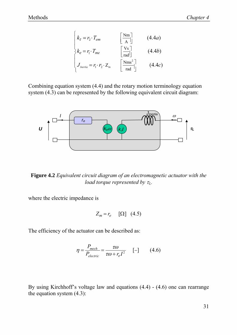
Combining equation system (4.4) and the rotary motion terminology equation system (4.3) can be represented by the following equivalent circuit diagram:
τL
ω
U
I re
JInertia
keω kτI
Figure 4.2 Equivalent circuit diagram of an electromagnetic actuator with the load torque represented by τL.
where the electric impedance is
[ ] (4.5)m eZ r= Ω
The efficiency of the actuator can be described as:
2 [ ] (4.6)mech
electric e
PP r I
τωητω
−= =+
By using Kirchhoff’s voltage law and equations (4.4) - (4.6) one can rearrange the equation system (4.3):

Chapter 4 Methods
32
1 ( , ) [V] (4.7 )( , )
[Nm] (4.7 ) [Nm] (4.7 )
( , ) [ ] (4.7 )
Inertia
e
L
U k k a
k I J bk I c
d
τ
τ
τ
η ω τω ωη ω τ
ω ττη η ω τ
•
−
−− = ⋅
= +==
The efficiency in equation (4.7d) contains the efficiencies of the three involved components, inverter, electrical machine, and gear. The efficiency term can be rewritten:
( , , ) ( , ) ( , ) [ ] (4.8)sInverter EM GearU Iη η ω η ω τ η ω τ −= ⋅ ⋅
where ηInverter accounting the switching losses and diode voltage drops in the inverter as a function of the frequency ωs, ηEM accounting for the losses involved in the electrical machine, and ηGear taking care of the friction losses in the gear. The average value of the inverter losses is assumed to be constant, thus making the efficiency term, η in equation (4.8) a function of the torque and angular velocity.
In sections 3.3 and 3.4 the efficiencies of the gear, ηGear and the inverter, ηInverter were defined. The losses involved in the efficiency ηEM are described in the next section.
4.2.1 Loss Models The losses occurring in an electrical machine can be divided into copper or winding, iron, air friction, bearing friction, and permanent magnet losses. The winding conductor is often copper and therefore in this thesis the winding losses are the same as copper losses.
There are several references which are covering the losses occurring in conducting metal laminations, see for example [24] and [25]. The iron losses can be divided into three parts. The first part comes from the inherent reluctance of the iron. This loss mechanism is referred to as static hysteresis losses. The second part comes from the time variation of the supply current. This variation produces “small” local current loops on the iron core which will reduce the flux.

Methods Chapter 4
33
This loss phenomenon is referred to as eddy current losses. The last loss mechanism is called excess losses. The excess losses are local eddy current losses associated with domain wall motions in the material. The excess losses are negligible at lower frequencies.
The iron loss model that is used in this thesis has the following form:
,
2 22 2 2 1.5 1.5lamination [W] (4.9)
6 Dens ironiron e e e ef h f fm m m
wP k k B f k B f k k B f
σπρ
= + +
where the three terms corresponds to the hysteresis, eddy current and excess losses. The constants kf, kh and ke are found by curve fitting to given data from material manufacturers. The BBm denotes an average value of the flux density and fe the electric operation frequency. The conductivity, σ, of the iron can also be found from curve fitting to manufacture loss data. The terms wlamination and ρDens,iron are lamination thickness and iron density respectively.
The copper losses can be divided into DC-losses (independent of the frequency) and the AC-losses (frequency dependent). The DC-losses comes from the resistivity of the copper, opposing the current flow. The AC-losses, known as eddy current losses, originate from the locally induced current loops in the copper. In a PM electrical machine there are two separate sources of eddy currents related to the copper losses. The first one originates from the skin effect. In this way the effective cross section area for current passage is decreased. The second part of the eddy currents originate from the alternating magnetic field that will induce current loops in the copper, see Figure 4.3. The analytical models for the eddy current losses in a conductor and the skin depth definition are derived in numerous references see for example [26].

Chapter 4 Methods
34
B B
(i) (ii) (iii)
Current Distribution
Current concentrations
Figure 4.3 Contour plots of current distribution in a circular conductor, caused by (i) the skin effect (ii) an external alternating field. (iii) The current
distribution with minimum in the middle of he conductor.
The losses originating from the alternating current can be superposed to the DC losses, as a correction term, see equation (4.10),
2 [W] (4.10)Cu AC DC rmsphP N k R I= ⋅
where the Nph denotes the number of the phases, kAC the correction factor for AC-losses (Alternating Current), RDC the resistance of the phase winding, and Irms the RMS current. The resistance of the copper is:
, [Ω] (4.11)Cu
CuDC Res Cu
lRA
ρ=
where ρRes,Cu is the resistivity of the copper, lCu the length of the winding and ACu cross sectional area of winding copper. The copper resistance is temperature dependent, see also [30], which can be expressed as
( )( )8 3, 1.72 10 1 20 3.9 10 [Ωm] (4.12)Res Cu CuTρ − −⋅= ⋅ + − ⋅ ⋅
where TCu is the conductor temperature. The correction factor kAC comprises two parts, one originating from the active part of the conductor and one from the end windings.

Methods Chapter 4
35
, , (4.13)AC AC active AC airk k k= +
The correction factor according to equation (4.13) is derived and expressed in terms of the reduced conductor height, defined in equation (4.15), in [27]. Simplified correction factors pointed out in the equation system (4.14) are given in [28] :
24
24
,
,
0.21 0.59 (4.14 )
9
0.81 0.59 1 (4.14 )36
activeAC active
activeAC air
c
c
Lmk aL
Lmk bL
ξ
ξ
⋅
⋅
⎧ ⎛ ⎞⎪ ⎜ ⎟⎜ ⎟⎪ ⎝ ⎠⎨
⎛ ⎞⎛ ⎞⎪⎜ ⎟⎜ ⎟⎪ ⎜ ⎟ ⎜ ⎟⎝ ⎠ ⎝ ⎠⎩
−= + ⋅
−= + ⋅ −
m is the number of conductor layers in the slot, the factor 0.59 is compensation for circular conductors, ξ is the “reduced conductor height”, Lactive is the active part of the conductor and Lc is the total conductor length. The term ξ is defined as
0
,(4.15)
Res Cu
efnb ha
πμξρ
= ⋅ ⋅
where n is the number of conductors in each layer, b is the conductor width, h is the conductor height, a is the slot width, and μ0 is the vacuum permeability.
The copper losses due to an alternating magnetic field (i.e. field variation due to the rotating rotor with permanent magnets) can be expressed in terms of the magnetic flux penetrating the copper. This loss is independent of the stator current and can also occur at no-load. The magnetic flux penetrating the copper windings comes mostly from the leakage flux in the stator core. This is a result of the wide stator teeth which attracts most of the air gap flux. The leakage flux density from the rotating magnetic field, see [28],[29], or [31], can be written as:
, ,2 2( ) sin( ) cos( ), [leak m m mleak n leak tB B t n B t tt ω ω T] (4.16)ω ⋅ ⋅= +
where BBleak,n and Bleak,t denote RMS amplitude of the normal respective tangential components of the magnetic flux densities, t is the time, and ωm is the
Chapter 4 Methods
36
mechanical angular frequency. Introducing a cylindrical coordinate system the equation (4.16) can be re-written:
( )( )
,n ,t
,n ,t
,( ) 2 sin( )cos( ) cos( ) sin( )
sin( )( sin( )) cos( )cos( ) [T] (4.17)
,leak m m mleak leak
m mleak leak
B B t B t R
B t B t
t ϕ ω ϕ ω ϕ
ω ϕ ω ϕ ϕ
ω = ⋅ + ⋅ +
− + ⋅
where ϕ is the angular coordinate. Applying the Faraday’s law to equation (4.17) and Ohm’s law, we get:
( ) 2,n ,tRe ,
Am
2 cos( )sin( ) sin( ) cos( ) (4.18)mz m mleak leak
s Cu
RJ B t B tω ω ϕ ω ϕρ
⋅ ⎡ ⎤⋅ ⎢ ⎥⎣ ⎦= − − ⋅
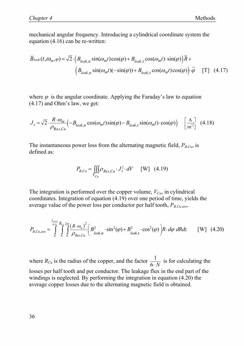
The instantaneous power loss from the alternating magnetic field, PB,Cu, is defined as:
2, , [W] (4.19)
CuB Cu zRes Cu
VP J dVρ= ⋅ ⋅∫∫∫
The integration is performed over the copper volume, VCu, in cylindrical coordinates. Integration of equation (4.19) over one period of time, yields the average value of the power loss per conductor per half tooth, PB,Cu.ave.
( )6
0 0 0
222 2 2 2
, ,, ,n ,t
sin ( ) cos ( ) [W] (4.20)active
Cu
LN
mB Cu ave
Res Cu
R
leak leak
RP B B R d dRdzπ ω ϕ ϕ ϕρ
⋅ ⋅ ⎛ ⎞⎜ ⎟⎝ ⎠
= + ⋅ ⋅⋅∫ ∫ ∫
where RCu is the radius of the copper, and the factor 16 N⋅
is for calculating the
losses per half tooth and per conductor. The leakage flux in the end part of the windings is neglected. By performing the integration in equation (4.20) the average copper losses due to the alternating magnetic field is obtained.

Methods Chapter 4
37
( )2 4
2 2, ,
,, , [W] (4.21)
22 4 6
m activeCuB Cu ave
Res Culeak n leak t
R LP B BN
π ωρ
⋅ ⋅⋅= +
⋅ ⋅ ⋅ ⋅
By calculating an average value of the BBleak,n and Bleak,tB for one half tooth and summing the average power loss over all teeth, equation (4.21) can be re-written:
( )2 42
2 2
1, ,
,, , , ,( ) ( ) [W] (4.22)
22 4 6
Km activeCu
B Cu totRes Cu
ave leak n ave leak ti
R Li iNP B B
Nπ ω
ρ=
⋅ ⋅ ⋅⋅= ⋅ +
⋅ ⋅ ⋅∑
where i denotes the tooth number, K the number of teeth, PB,Cu,tot the average total power losses, N the number of conductors per half tooth, and BBave,leak,n and Bave,leak,tB the average leakage flux densities.
The air friction of the stabilizing bandage around the magnets in the air gap is given by [29]:
3 4, ,, [W] (4.23)Dens Force air Rotorfriction air Rotor bandmfP C R Lρ π ω += ⋅ ⋅
where ρDens,Force,air is the density force of air
( ,, , 3 29.81 (4.24)Dens airDens Force airkg mm s
ρ ρ ⎡ ⎤ ⎡ ⎤⋅⎢ ⎥ ⎢ ⎥⎣ ⎦⎣ ⎦= ⋅ ), ωm the mechanical angular
velocity, RRotor+band the radius of the rotor plus the bandage, and LRotor the length of the cylinder. The friction coefficient Cf is dependent of the geometrical dimensions of the rotor cylinder, the air flow and the composition of the air. The air flow could be either laminar, turbulent or in transition state. The transition state is not considered in this project. Turbulent flow gives a higher value of Cf, i.e. higher friction losses. The fact that the rotor is enclosed by the stator has to be considered in the determination of the friction coefficient Cf. The empirical friction coefficient is expressed as:
0.34
0.5
0.34
0.2
10.515 500 10 (4.25 )
10.0325 10 (4.25 )
Rotor
Rotor
gg
gf
gg
g
LRe a
R ReC
LRe b
R Re
⎧ ⎛ ⎞⎪ ⎜ ⎟⎜ ⎟⎪⎪ ⎝ ⎠⎨⎪ ⎛ ⎞
⎜ ⎟⎪ ⎜ ⎟⎪ ⎝ ⎠⎩
⋅ ∀ < <=
⋅ ∀ ≥

Chapter 4 Methods
38
where Lg is the air gap length, and Reg is the Couette Reynolds number,
(4.26)Rotor
air
g mg
L RRe
ων
=
with the kinematic viscosity of air, υair .
Permanent magnets can also be a source of losses. In magnets there are no hysteresis losses because of the linearity of the magnetization curve, i.e. the permeability of the magnet is close to 1. There are however three sources of eddy current losses due to the conductivity of the magnet material: The first part comes from the permeance variations in the flux path. Often there are air pockets in between the stator slot iron. The air and iron have different flux reluctances. When one magnet is placed such that it is covering both the air pocket and the stator slot, the flux pattern through the part facing the iron is higher than the part facing the air pocket. This could be seen as there are induced eddy currents on the magnet which is counteracting the effective flux. The first part of the magnet eddy current losses occurs at no-load.
MPM J
lPMhPM
bPM
RotorMagnet
Figure 4.4. Illustration of the geometry of the magnet.
The second and third part occurs at load. These two parts are related to the counteraction of the harmonics with the effective flux. The losses related to the harmonic contents of the flux in the air gap can be divided into time and space harmonics. The space harmonics are caused by the winding distribution. This distribution will cause an asynchronism of the current flux in the air gap. The harmonic content of the supply current will also have a counteracting influence on the effective air gap flux, denoted often as time harmonic permanent magnet losses.

Methods Chapter 4
39
These induced eddy currents or in fact the heat that is created from these can have a demagnetizing effect on the magnets. The first loss source can be reduced by increasing the air gap.
The current, is, as a function of time, t, from the inverter to the electrical machine contains harmonics,
00
, , ,( ) 2 2 cos( ) [A] (4.27)s ss s h s hh
i t I I h t zω ϕ>
⎛ ⎞⎜ ⎟⎝ ⎠
= + −∑
where Is,0 is the RMS DC-level of the current, Is,h the RMS value of the harmonic current amplitude, h the harmonic order, ωs, the angular frequency, and ϕs,h the phase shift of the respective harmonic. Pure sinusoidal harmonics is assumed and as a result the DC-level and phase shifts are set to zero. In the active part of the winding the current has axial direction, z
From Ampere’s law we know that a current carrying conductor gives rise to a circulating magnetic field, illustrated in Figure 4.5,
B
i
Figure 4.5 Illustration of Ampere’s law.
The windings of an electrical machine are distributed over some space, i.e. not located in one single point. This results in a harmonic magnetic field in the air gap, because of the superposition of the magnetic fields from each turn. The air gap magnetic flux density as a function of time can be divided into two parts, a radial R or normal n and an angular, ϕ or tangential t component according to:
( ) [T] (4.28)airgap n tRB t B R B B n B tϕϕ= + = +

Chapter 4 Methods
40
In Figure 4.6 the normal magnetic flux density and corresponding eddy current in a magnet are shown.
Bϕ
J
J
n R=
z
hPM
lPM
Figure 4.6 The magnetic flux density into the magnets with the corresponding eddy current density.
In a cross sectional view of the electrical machine the radial and normal components, and the angular and tangential components are the same. In equation (4.28) BBR denotes the radial RMS component of the magnetic flux density, BϕB the angular component of the magnetic flux density, BBn the normal magnetic flux density component, and BtB the tangential component of the magnetic flux density.
In [28] and [32] another approach is used for calculating the eddy current losses in the magnets than the below. In analogy with a conductor inside an alternating magnetic field we can write the air gap magnetic flux density in the angular direction as a function of the frequency of the supply current:
1,
3,
11 2
33 4
1 21 1
3 4
1
3
, ,
,1 1
2
( , ) sin( ) sin( )
2 cos( ) cos( ) [T] (4.2
,airap s sn h hh h
st h hh h
B t B h h t
B h h t
ϕ ϕ α ω
ϕ α ω
ϕ ω≥ ≥
≥ ≥
⎛ ⎞⎛ ⎞⎜ ⎟⎜ ⎟− ⋅ +⎜ ⎟⎜ ⎟⎝ ⎠⎝ ⎠⎛ ⎞⎛ ⎞⎜ ⎟⎜ ⎟
⎜ ⎟⎜ ⎟⎝ ⎠⎝ ⎠
= +
⋅ +
∑ ∑
∑ ∑ 9)
where BBn,h and Bt,hB are the harmonic RMS amplitudes of the magnetic flux densities in the air gap. The h1, h2, h3, and h4 denote the harmonic orders, ϕ the

Methods Chapter 4
41
angular coordinate variable, ωs the angular frequency, and α1, and α3 the phase shifts. Applying the Faraday’s law on equation (4.29) yields
21,
43,
11 2
33 4
1 21 1
3 4
1
3
,
,1 1
2
V m
sin( ) cos( )
2 cos( ) sin( ) (4.30)
s sn h hh h
s st h hh h
zE R B h h h t
R B h h h t
ω ϕ α ω
ω ϕ α ω
≥ ≥
≥ ≥
⎛ ⎞⎛ ⎞⎜ ⎟⎜ ⎟⋅ − ⋅ ⋅ +⎜ ⎟⎜ ⎟⎝ ⎠⎝ ⎠⎛ ⎞⎛ ⎞ ⎡ ⎤⎜ ⎟⎜ ⎟⋅ ⋅ ⋅ ⎢ ⎥⎜ ⎟⎜ ⎟ ⎣ ⎦⎝ ⎠⎝ ⎠
= ⋅ +
⋅ + −
∑ ∑
∑ ∑
with the radial coordinate R, and the electric field Ez. By expressing the electric field intensity as a current density with the help of Ohm’s law and integrating the instantaneous power loss over one period of time yields
( )
( )
1,
33,
2
11 2
4
33 4
2 2
11 1
2 2
3
1
3
2
, ,,
2
,
,
,1 1
22
W 2 m
sin( )
2 cos( ) (4.3
PM Dens aveRes PM
Res PM
sn h h
h h
st h h
h h
hRP B h
hR B h
ω ϕ α
ω ϕ α
ρ
ρ
≥ ≥
≥ ≥
⎛ ⎞ ⎛ ⎞⎜ ⎟ ⎜ ⎟⋅ − ⋅ +⎜ ⎟ ⎜ ⎟⎝ ⎠ ⎝ ⎠
⎛ ⎞ ⎛ ⎞⋅ ⎡ ⎤⎜ ⎟ ⎜ ⎟⋅ ⎢ ⎥⎜ ⎟⎜ ⎟ ⎣ ⎦⎝ ⎠⎝ ⎠
⋅= +
⋅ +
∑ ∑
∑ ∑ 1)
where PPM,Dens,ave denotes the average power loss density, and ρRes,PM the resistivity of he permanent magnet. By integrating equation (4.31) over the dimensions of one magnet in cylindrical coordinates we get:
, , ,0
[W] (4.32)PM PM
PM ave PM Dens ave
h R l
RP P R dRd dz
α
αϕ
+
−= ⋅ ⋅∫∫ ∫
where
2
2
arctan [rad] (4.33)PM
PM
b
lRα
⎛ ⎞⎜ ⎟⎜ ⎟⎛ ⎞⎜ ⎟+⎜ ⎟⎜ ⎟⎝ ⎠⎝ ⎠
=
Neglecting the cross terms of the summations in equation (4.31) and performing the integration in equation (4.32) yields:

Chapter 4 Methods
42
( ) ( ) 3 4 1 2 1 1
2 4
42 2 242
1 11 3
2,
,
, ,2 2
2 [4
PMPM ave PM
h hRes PM
sn h t h
h h
h hR l RP B Bh ω αρ ≥ ≥≥ ≥
⎛ ⎞⎛ ⎞ ⎛ ⎞⎛ ⎞ ⎛ ⎞−⎜ ⎟⎜ ⎟ ⎜ ⎟⋅ ⋅ ⋅ +⎜ ⎟ ⎜ ⎟⎜ ⎟⎜ ⎟⎜ ⎟ ⎜ ⎟⎜ ⎟⎝ ⎠⎝ ⎠⎝ ⎠ ⎝ ⎠⎝ ⎠
+≈ ∑ ∑∑ ∑ W] (4.34)
)
By taking the first term of the Taylor series expansion of equation (4.33), moving the magnet coordinates to the origin of the cylindrical coordinate (i.e.
0 [m] (4.35R = ), and simplifying equation (4.34) we get the average eddy current losses per magnet:
( ) ( )2
,2 4 1 3
3 4 1 2
3 2 2 2,
1 1
2
1 1 , , [W] (4.36)
4PMRes PM
sPM ave PM PM n h t h
h hh hP b l B h B hh ω
ρ ≥ ≥≥ ≥⋅
⎛ ⎞⎛ ⎞ ⎛ ⎞⎜ ⎟⎜ ⎟⋅ ⋅ ⋅ ⋅ + ⋅⎜ ⎟
⎜ ⎟⎜ ⎟⎜ ⎟⎝ ⎠⎝ ⎠⎝ ⎠≈
⋅ ∑ ∑∑ ∑
In the references [28], [29], and [32] the normal component of the air gap magnetic flux density is studied. In this way the eddy current losses are proportional to . In the derivation of the equation (4.36) the angular component of the magnetic flux density is considered. As a result the induced eddy current loops are different than the ones from the references mentioned
above and thereby the factor .
3 2PM PMb l B
2 4 1 3 3 4 1 2
2 2
1 1
3 2
1 , ,PM PM n h t h
h hh hb l B h B h
≥ ≥≥ ≥
⎛ ⎞⎛ ⎞ ⎛ ⎞⎜ ⎟⎜ ⎟ ⋅ + ⋅⎜ ⎟
⎜ ⎟⎜ ⎟⎜ ⎟⎝ ⎠⎝ ⎠⎝ ⎠∑ ∑∑ ∑ 2
1
The bearing friction losses of an electrical machine are proportional to the angular mechanical velocity, ωm, and the load torque, τL, see [30]:
20
,,
4
( )[W] (4.37)friction bearing
m mLfriction bearing DP
μ τ τ ω⋅ + ⋅=
In equation (4.37) the bearing friction coefficient is µfriction,bearing, τL is the load torque, τ0 denotes the pre-load torque, and Dm denotes the average bearing diameter.

Methods Chapter 4
43
4.2.2 Modeling of the Permanent Magnet The relations between the magnetic flux, B , magnetic field, H , magnetization density, M , and surface current density, J , for a permanent magnet material are
( )2
0
Am
[T] (4.38 )
(4.38 )
B H M a
J M b
μ
⎡ ⎤⎢ ⎥⎣ ⎦
= +
=∇×
One way of modeling a permanent magnet is by circulating current, see Figure 4.7. By assuming that the magnetization density inside the magnet is uniform the contribution from the neighboring atomic dipoles will cancel out. The contribution to the magnetization comes from the edges where no cancellation occurs. Because of the cancellation effects inside the magnet the equation (4.38b) can be re-written according to
Am
(4.39)sJ M n ⎡ ⎤⎢ ⎥⎣ ⎦
= ×
with the line current density sJ and the unit normal vector n .
M n n
Js,y
Js,y
Figure 4.7 Permanent magnet model, with the magnetization M and line current density Js,y.
Equation (4.39) has one dimension less than the quantities in the equation (4.38a). Therefore a simplification of equation (4.38a) can be done.

Chapter 4 Methods
44
,
AmAm
(4.40 )
(4.40 )
zz z
o
s y z
BM H a
J M b
μ⎡ ⎤⎢ ⎥⎣ ⎦
⎡ ⎤⎢ ⎥⎣ ⎦
= −
=
The linearity and isotropic behavior of the magnets allows us to set the magnetization equal to the coercive force, Hc of the magnet:
( )0 [T] (4.41)z r z cB H Hμ μ= +
where μr is the relative permeability. Rearrangement of equation system (4.40) and equation (4.41) gives:
,Am
( 1) (4.42)s y r c rJ H Hμ μ ⎡ ⎤⎢ ⎥⎣ ⎦
= + −
In magnets the value of relative permeability is close to unity and therefore the second term in equation (4.42) can be neglected and the line current density can be set equal to the coercive force. The magnetization of the magnet is now expressed in terms of line current density, see [31]. Integration of the line current density over the height of the magnet, lPM, give us the circulating “current”, I, on the edges of the magnet. Rearranging the equation (4.42) gives:
, [A] (4.43)s y cPM PMI J l H l= ⋅ = ⋅
Rectangular permanent magnets can be modeled in a FEM-program as an area with the relative permeability μr close to 1 with two small source areas on the edges of the magnet with the current from equation (4.43), see Figure 4.8.
lPM Mz-I+I
xΔ xΔ
Figure 4.8 Permanent magnet model.
Methods Chapter 4
45
The length of the areas, xΔ , where the current is applied can be around 0.1 [mm]
4.3 Optimization of the EMA
One first assumption can be that the efficiencies of the involved parts of the EMA are uncoupled, i.e. independent. In that way the different parts can be optimized separately.
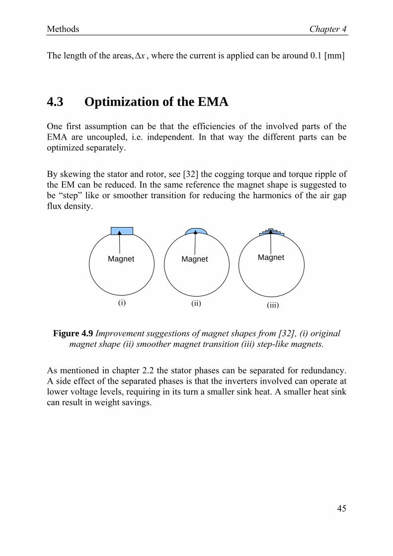
By skewing the stator and rotor, see [32] the cogging torque and torque ripple of the EM can be reduced. In the same reference the magnet shape is suggested to be “step” like or smoother transition for reducing the harmonics of the air gap flux density.
(i)
Magnet
(ii)
Magnet
(iii)
Magnet
Figure 4.9 Improvement suggestions of magnet shapes from [32], (i) original magnet shape (ii) smoother magnet transition (iii) step-like magnets.
As mentioned in chapter 2.2 the stator phases can be separated for redundancy. A side effect of the separated phases is that the inverters involved can operate at lower voltage levels, requiring in its turn a smaller sink heat. A smaller heat sink can result in weight savings.


Results Chapter 5
47
Chapter 5 Results
5.1 Introduction
The result of this project is divided into two parts, one is from the 2D FEM (2 Dimensional Finite Element Method) and the other is from the simplified equivalent circuit simulation of a MEA power system. In the FEM analysis the induced-no-load voltage and the output torque of the involved EM are calculated. From these calculations the counter EMF (Electro Motive Force) and torque constant are condensed. The flux density values are also used in different loss calculation for the estimation of the efficiency. In the second part of the simulations the equation system (4.7) is implemented in the object oriented language Modelica.
5.2 2D FEM Analysis of the Electrical machine
There are numerous references regarding the basic FEM calculations, see for example [33]. The magnetic properties of the materials involved are required for a FEM analysis.
The surface mounted radial PMSM with concentrated windings, from SPAB (Stridsberg Powertrain AB), studied in this thesis has promising properties regarding the MEA application. The novelty lies in combination of many poles, supporting stator tooth, concentrated winding arrangement resulting in a high power density and high torque production. This electrical machine has 6 phases and 20 poles. The concentrated winding arrangement reduces the end-winding effect and copper losses. The supporting teeth between the stator phases have a “cooling” effect on the windings near the support tooth. The thermal behaviour of this machine is further analyzed in chapter 6.1. The lower temperature

Chapter 5 Results
48
decreases the copper losses. The “high” number of magnets (i.e. poles) used on the rotor surface has a positive effect on the toque production. The output torque is also proportional to the flux density in the air gap. The magnets are placed on the surface of the rotor which means low saliency, in another words the reluctance along the flux path is nearly the same in both d and q directions, which in its turn means cogging and ripple torque reduces. Another benefit of this electrical machine is the modularity of the machine. By stacking more laminations the output power can be increased. The assembly allows therefore a high torque output with relatively low angular velocity and losses. The studied machine delivers 1 [kW] at 2250 [rpm], with radius 97 [mm] and length 22 [mm]. The inverter used is one H-bridge for each phase. The three stator teeth in each phase are connected in series. The number of turns is 30. In Figure 5.1 an X-ray image of the studied EMA is shown.
Bearings
Gear
Stator
Rotor
Heat sink flanges
Figure 5.1 The studied compact EMA from the aircraft manufacturer SAAB AB and SPAB.
The winding arrangement of the studied electrical machine with six phases (A-F) is
A-A -AA A-A -BB B-B -BB C-C -CC C-C -DD D-D -DD E-E -EE E-E -FF F-F -FF
A cross sectional picture of the involved electrical machine is shown in Figure 5.2 where placement and order of phase A is pointed out.

Results Chapter 5
49
Iron Copper
UpperAir
A -A
Lower ABack -A A
-A -B F
Magnet
Figure 5.2 Cross-sectional view of the studied 6-phase, and 20 pole EM from SPAB. The current sign and order of the phase A is pointed out. The upper,
back, and lower part of the core is also pointed out.
The involved materials in the electrical machine have the following physical properties:
Table 5.1. Physical properties of the involved materials.
Material ρdensity 3kgm⎡ ⎤⎢ ⎥⎣ ⎦
μr [-] Hc kAm
⎡ ⎤⎢ ⎥⎣ ⎦
ρresistivity 810 m−⎡ ⎤Ω⎣ ⎦
Iron 7650 Figure 5.3 - 44 Copper - 1 - Equation (4.12) Air 1.27@ 20
[ºC] 1 - -
Magnet (NdFeB)
7800 1.1 850 64
Insulation - 1 - -
The core material used in the EM is M330-35A from Surahammars Bruk and has the static and dehysterized magnetization curve shown in Figure 5.3.

Chapter 5 Results
50
Figure 5.3 The dehysterized magnetization curve of the material M330-35A from Surahammars Bruk at 50 [Hz].
The values of the magnetization curve in Figure 5.3 are measured at 50 [Hz]. This can be a source of error in the FEM calculations. However an EMA is often operated at low frequencies and therefore this error is neglected here.
The no-load flux lines are illustrated in Figure 5.4. The concentrated winding arrangement in combination with the supporting teeth between the stator phases, the wide stator teeth and the high number of rotor poles, makes the flux paths short and broad, which in its turn decrease the core losses and the leakage flux between the magnets. This assemble makes it also possible to decrease the stator ‘head’ core size. The flux lines divide in the ‘head’ of the core and no flux concentrations can be noted in these regions as would be expected because of the area differences in the back and head of the core. In Figure 5.4 the no-load contour plot of the magnetic vector potential is shown.
In Figures 5.5 and 5.6 the normal component of the air gap flux density is shown. The amplitude is close to 1.2 [T]. This high value will naturally effect the torque production in a positive sense. The effect of slot openings is shown in Figure 5.6.

Results Chapter 5
51
Figure 5.4 The no-load equi-potentials of flux density and the contour plot of the magnetic vector potential, Aϕ.
Figure 5.5 The normal component of the magnetic flux density in the air gap at no load, Bn.
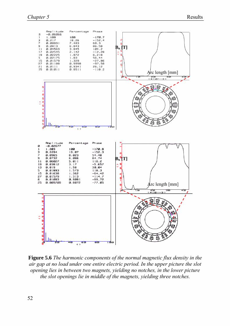
Chapter 5 Results
52
BBn [T]
Arc length [mm]
Figure 5.6 The harmonic components of the normal magnetic flux density in the air gap at no load under one entire electric period. In the upper picture the slot opening lies in between two magnets, yielding no notches, in the lower picture
the slot openings lie in middle of the magnets, yielding three notches.
Arc length [mm]
BBn [T]

Results Chapter 5
53
The cost of the permanent magnets comprise both the material itself and the manufacturing of appropriate shapes. In a machine design the magnet size and shape then has to be optimised. In the studied electrical machine the effort has been focused on the high torque output. Therefore NdFeB magnets have been used, with a high coercively force and smoothed rectangular cross sectional shapes. Having this in mind the amount of magnet used in the machine can be optimized further, see [32]. In this reference a smoother transition, see Figure 4.9, or step-like cross section instead of rectangular cross section shape is suggested. In this way the harmonic component of the magnet flux can be reduced.
In FEM models of an electrical machine there are two ways of calculating the resulting torque, the first one uses the Maxwell stress tensor and the second one is based on the principle of virtual work. The derivation of both methods can be for example found in [24] and the FEM-formulations in [34].
The Lorentz’s force relation is the basic physical law that is used for the derivation of the both relations mentioned above. A current carrying conductor exposed to an external magnetic field senses a force, illustrated in Figure5.7.
i
B
B
F
Figure 5.7 Illustration of the Lorentz’s force
The derived force vector based on the Maxwell stress tensor is:
( )2 2
0
Nm
1 1 (5.1)2 n t n t dF B B n B B t
μΓ
⎛ ⎞ ⎡ ⎤Γ⎜ ⎟ ⎢ ⎥⎣ ⎦⎝ ⎠= − +∫
where the flux density is expressed in a normal and a tangential component:

Chapter 5 Results
54
[T] (5.2)n tB B n B t= +
n is the unit vector in the normal direction and t is the unit vector in the tangential direction. The integration path Γ is preferably placed in the middle of the air gap in FEM calculations, however the analytical expression assumes a path just outside the rotor body (in the non-ferromagnetic material). The rotating resulting torque around the origin of the rotor can be expressed in terms of the tangential component of the force vector:
( )0
Nmm
1 (5.3)Rotor n tR B B t dτμΓ
⎡ ⎤× ⎢ ⎥⎣ ⎦= Γ∫
with RotorR defined as the distance vector in the radial direction from the origin of the rotor. The FEM calculations are often performed in 2-D, that is why the force and torque vectors are expressed per axial length unit. Therefore it is often enough to multiply these values by the effective axial length of electrical machine (i.e. the rotor length), because of the uniformity of the flux density in the rotor axial direction. The flux uniformity is only valid inside the rotor body and not in the ends where the flux will deviate. If the performed FEM-calculations are done over one pole, then the resulting torque and force have to be multiplied by the number of poles as well. The magnitude of the rotating torque vector that can be calculated in a FEM program is
, ,
0[Nm] (5.4)n i t i
Rotor Rotor ii
B BR Lτ
μ= ΔΓ∑
with LRotor, the axial length of the rotor. The integration is replaced by summation and the rotor cross sectional area is divided in ‘mesh’ elements in ordinary FEM calculation manner, with BBn,i and Bt,iB denoting the flux densities in the mesh element number i, and iΔΓ the i:th part of the corresponding path in the air gap.
The second way of expressing the torque is by using the principle of virtual work. The underlying idea is that because the magnetic energy is conservative, the force can be expressed as the difference of energies at the two points divided by the path difference. The conservative means in this case that the force is dependent of the path difference and not the path itself. Expressing this in

Results Chapter 5
55
mathematical terms means that the force Fs can be expressed in terms of magnetic energy W, according to:
0
Nm
(5.5)B
Vs
WF H dB dVs s
⎛ ⎞⎛ ⎞ ⎡ ⎤⎜ ⎟⎜ ⎟ ⎢ ⎥⎜ ⎟⎜ ⎟ ⎣ ⎦⎝ ⎠⎝ ⎠
∂ ∂= − = −∂ ∂ ∫∫∫ ∫ i
Equation (5.5) is valid under the assumption that the flux in the system is constant, i.e. no induced EMF from time varying flux will contribute to the magnetic energy. If in the other hand the current into the system is constant, the force equals the magnetic energy difference at two points divided by the path length between the two points without the negative sign, see also [35].
Expressing equation (5.5) in a cylindrical coordinate system yields:
Nm
1 (5.6)Rotor
s I constWF
R ϕ=⎡ ⎤⎢ ⎥⎣ ⎦
∂=∂
with the radius R and angle ϕ. The uniformity is used along the axial direction, which means that the volume integral, in equation (5.5), becomes a surface integral times the axial length of the machine. The rotating torque around the centre of the machine can be expressed as:
Nm (5.7)mRotor sR Fτ
⎡ ⎤⎢ ⎥⎣ ⎦
=
In the same way as previously the integration is replaced by summation and the derivative is replaced by a difference. The resulting torque is:
2 1
,2 ,2 ,2 ,1 ,1 ,12 1, ,[Nm] (5.8)
Rotor Rotor RotorRotor
i i i i i ii i
Rotor
s
i i
W WR F R LR
H B R H B RL
τϕ
ϕ ϕ
ϕ
−
=
−= = ⋅ =⋅Δ
⋅Δ ⋅Δ ⋅Δ ⋅Δ ⋅Δ ⋅Δ
Δ
∑ ∑

Chapter 5 Results
56
where W2 and W1 are the total magnetic energies in two rotor positions with the angle difference ϕΔ , and i is the mesh element number. BΔ , RΔ , and ϕΔ are defined as the difference of the respective quantity for the neighbouring mesh elements.
The attraction between the magnets and the stator teeth at no-load will create a cogging ripple, see Figure 5.8.
Figure 5.8 The cogging torque of the studied machine.
From Faraday’s law we know that a moving conductor inside a magnetic field will be exposed to the induced voltage, e
[V] (5.9)dedtΨ= −
When we are dealing with a number of conductors, a winding arrangement, the resulting flux linkage,Ψ , can be expressed as the flux, ϕ enclosed by each turn times the number of turns, N. The latter relation can be used because of the flux going through one turn can be assumed to enter the other turns as well, (i.e. no leakage).

Results Chapter 5
57
[V] (5.10)d de Ndt dt
ϕΨ= − = −
For better understanding the physics behind equations (5.9)-(5.11) the references [24] or [35] can be used. The magnetic flux through a closed path, C can be expressed as the line integration of the magnetic vector potential, A along the path.
[ ] (5.11C
A dl Wbϕ = ∫ )i
In Figure 5.9 an example of integration path is shown for the calculation of the flux going through the stator core resulting in induced voltages on the winding surfaces. The end windings along the integration path, C, have negligible contribution to the integral, (i.e. a small leakage flux). Therefore the integral along the lines 3 and 4 are set to zero.
ϕ
4
21
3
Windings
Iron
C C
Figure 5.9 The integration path (pink) along the active part of the windings, circumscribing the flux in the iron. Also the winding cross sectional areas
(brown) where average values of the magnetic vector potentials are calculated are shown.
Using an average value of the magnetic vector potential in equation (5.11) was suggested in [36]. The magnetic vector potential is constant in the axial direction in the winding. In [37] an example is given for calculating the flux linkage based on the average value of the magnetic vector potential in an electrical machine context. An average value, Aave, of the magnetic vector potential, A , can be calculated by:

Chapter 5 Results
58
Wbm
(5.12)Save
S
A dsA
ds⎡ ⎤⎢ ⎥⎣ ⎦
⋅=∫∫∫∫
The integration surface, S, is the winding cross section area, shown in Figure 5.8. Having this in mind we can reformulate equation (5.11):
( )2, 1, Wb (5.13)Rotor ave aveL A Aϕ − ⎡ ⎤⎣ ⎦= ⋅
Applying equation (5.14) on the studied electrical machine with concentrated winding arrangement, the flux linkage per phase,ΨΘ, can be calculated as a function of the mechanical angle of the rotor (i.e. rotor position), Θ :
( ) ( )13
, ,2 1 , ,21
1 Vs (5.14)Rotori
ave i ave ii
N L A A−Θ Θ − Θ
=
⎛ ⎞⎜ ⎟ ⎡ ⎤⎣ ⎦⎜ ⎟⎝ ⎠
−Ψ = ⋅ ⋅ −∑
where N denotes the number of turns per tooth, LRotor the effective length of the machine, AΘ the average value of the magnetic vector potential induced at no load on the winding cross section. The relation for a distributed winding arrangement that is discussed in [37] is modified in equation (5.15) for a series connected concentrated winding arrangement, with three stator teeth. The flux linkage per phase for a concentrated winding electrical machine can be expressed as a sum of the average values of the magnetic vector potential of the three stator teeth (series connected winding) multiplied by the number of turns and effective length of the rotor.
In Figure 5.10 the winding cross sectional areas where the average values of the magnetic vector potentials for phase A are calculated are pointed out.

Results Chapter 5
59
Figure 5.10 The winding cross sectional areas where the average values of the magnetic vector potential of the phase A are calculated.
Figure 5.11 The flux linkage for phase A, one electric period, with effective length LRotor = 22 [mm] and N = 30.
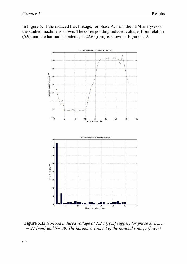
Chapter 5 Results
60
In Figure 5.11 the induced flux linkage, for phase A, from the FEM analyses of the studied machine is shown. The corresponding induced voltage, from relation (5.9), and the harmonic contents, at 2250 [rpm] is shown in Figure 5.12.
Figure 5.12 No-load induced voltage at 2250 [rpm] (upper) for phase A, LRotor = 22 [mm] and N= 30. The harmonic content of the no-load voltage (lower)

Results Chapter 5
61
The counter EMF constant can now be calculated, at the base velocity 2250
[rpm]. For the velocity of 236 rads
⎡ ⎤⎢ ⎥⎣ ⎦
(60
22502 2π π= ⋅37.5=236 rads
⎡⎢⎣ ⎦
⎤⎥ (5.15))
and the RMS value of the phase voltage 752
related to the fundamental
frequency from Figure 5.12, yields:
Vsrad
75 0.225 (5.16)2
12 37.5
rmse
Vkω π
⎡ ⎤⎢ ⎥⎣ ⎦
= = ⋅ =⋅
From Table 2.1 the maximum power needed for actuators is close to 1 [kW]. If the efficiency of the 6 phase electrical machine plus screw mechanism is 0.85 then the RMS value of the phase currents, with a phase voltage 75 [V], is
31 10 1 2 3.7 [A] (5.17)0.85 6 75rmsI ⋅= ⋅ ⋅ =
In Figures 5.13 and 5.14 the torque produced by the machine is calculated by FEM simulations, for 27.5, 15, 3.7, and 1.5 [A RMS].
Irms=27.5 [A], 3600 [rpm]
Irms=3.7 [A], 2250 [rpm]
Irms= 1.5 [A], 3600 [rpm]
Figure 5.13 2D FEM torque calculations at 13.5, 1 and 0.9 [kW].

Chapter 5 Results
62
The angular speed is set to 2250 [rpm] for the FEM calculation with 3.7 [A] and 3600 [rpm] for the rest in Figure 5.13. In Figure 5.14 the torque production is shown, for 10° to 360° phase lags between the rotor position and the reference phase current. The legend of the figure shows the average values of the torque production along the rotor rotations in synchronism with the phase currents. In the motor-mode the electrical machine should be operated around these points for maximum torque production. Observe that Figure 5.14 shows both the motor and generator mode of operation.
τave=20.7 [Nm]
τave=20.5 [Nm]
Figure 5.14 2D FEM calculations of the torque at 7.5 [kW], RMS phase current 15 [A], 3600 [rpm].
The analytical expressions (5.4) and (5.7) for calculating the resulting torque in an electrical machine can be rewritten, see also [34] or [37]:

Results Chapter 5
63
( ) ( )2
(1),2sin [Nm] (5.18)
2rmsRotor Rotor airgap windFactor
Rotor g
R L B N I k QR L
πβ
πτ
⋅ ⋅ ⋅ ⋅ ⋅= ⋅
+
In equation BB(1),airgap is the fundamental RMS value of the air gap flux density, N is the number of turns per slot, Irms is the phase RMS current, kwindFactor is the winding factor, Q the number of slots, and β is the angle between the stator current vector and the magnet flux.
According to [38] the winding factor of a 20 pole (p) and 18 stator teeth (Q) machine with concentrated windings is 0.945. With the values BB(1),airgap = 1.2 0.85
2= [T], N = 30, Irms = 27.5, 15, 3.7 and 1.5 [A], kwindFactor = 0.945, Q =
2⋅18, RRotor = 69.04 [mm], LRotor = 22 [mm], Lg = 1 [mm], and β =2π for a non-
salient machine, the torque values of the machine are 35, 18, 5, respectively 2 [Nm]. The factor 2 in front of the number of stator teeth comes from the correction for the concentrated winding arrangement, two windings per slot.
The torque constant can now be calculated at 3.7 [A] phase current:
NmA
5 1.35 (5.19)3.7rms
avekIττ ⎡ ⎤
⎢ ⎥⎣ ⎦
= = =
The inductance, Ltot, of the winding is defined as
22 [H] (5.20)tot
WLI⋅=
where the magnetic energy, W, was discussed previously, see for example [39] for the derivation of the inductance. In surface mounted PM machine the total inductance, Ltot, is twice the Ld and Lq, because of the non-saliency. If the end-effects of the windings are neglected, the inductance of the windings in the studied electrical machine can be calculated by
2 [H] (5.21)qdWL LI
≈ ≈

Chapter 5 Results
64
In Figure 5.15 the total, d, and q inductances are shown. The simulation is done when the current is applied to the respective phase winding and ‘rotated’ in synchronism with the rotor movement. The magnet flux density is set to zero for the calculations of the magnetic energy at different rotor positions.
Ld ≈ Lq
Ltot
Figure 5.15 2D FEM calculations of the inductance where the d and q inductances coincide.
5.2.1 Losses The iron loss model constants in chapter 4.2.1 are based on the data from the manufacturer Surahammars Bruk AB, envisaged in Figure 5.16. Inserting these parameters in equation (4.9) for frequencies 0-1000 [Hz] and core flux densities between 0 and 1.8 [T] gives the core losses shown in Figure 5.17.

Results Chapter 5
65
Figure 5.16 The manufacturer loss data of the material M330-35A for supply frequencies 50,100, 200, 400 and 1000 [Hz].
f [Hz]
Figure 5.17 The stator core loss as function of magnetic flux density and supply frequency.
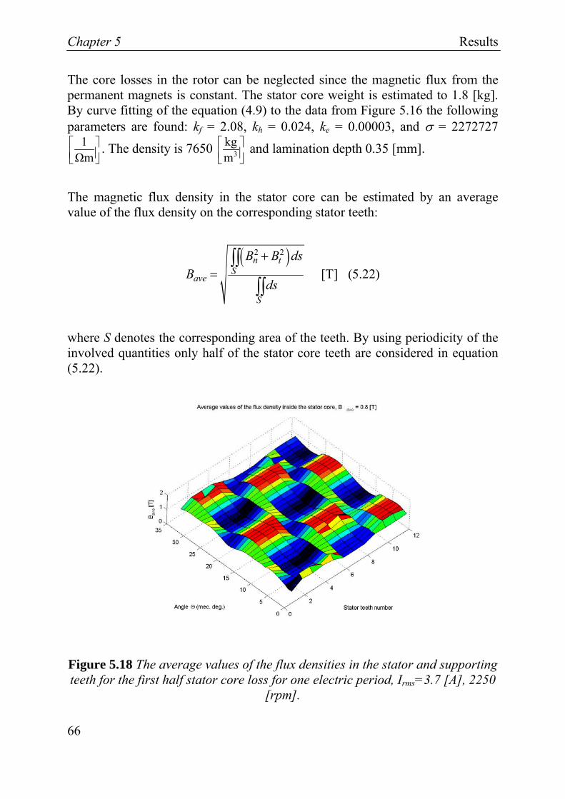
Chapter 5 Results
66
The core losses in the rotor can be neglected since the magnetic flux from the permanent magnets is constant. The stator core weight is estimated to 1.8 [kg]. By curve fitting of the equation (4.9) to the data from Figure 5.16 the following parameters are found: kf = 2.08, kh = 0.024, ke = 0.00003, and σ = 2272727
1Ωm⎡⎢⎣ ⎦
⎤⎥ . The density is 7650 3
kgm⎡⎢⎣ ⎦
⎤⎥ and lamination depth 0.35 [mm].
The magnetic flux density in the stator core can be estimated by an average value of the flux density on the corresponding stator teeth:
( )2 2
[T] (5.22)n t
Save
S
B B dsB
ds
+=∫∫
∫∫
where S denotes the corresponding area of the teeth. By using periodicity of the involved quantities only half of the stator core teeth are considered in equation (5.22).
Figure 5.18 The average values of the flux densities in the stator and supporting teeth for the first half stator core loss for one electric period, Irms=3.7 [A], 2250
[rpm].

Results Chapter 5
67
The average values of the magnetic flux density for one electric period and the three stator teeth for phases A, B, and C with supporting teeth in between is shown in Figure 5.18. The area of one stator tooth is 0.0005221 [m2] and the supporting tooth 0.0002016 [m2]. The periodicity of the magnetic flux density gives the ‘time’ average of the stator core teeth flux can be calculated by
36 122
1 1( , )
0.83 [T] (5.23)12 36
avej i
ave
B i jB = = ==
⋅
∑∑
Inserting the values from Figure 5.18 in equation (5.23) gives 0.83 [T] as average value of the flux density in the stator core. A better way of estimating the core losses would have been to divide the stator teeth in three parts, upper, middle, and lower part. The stator teeth dimensions of the studied electrical machine are smaller in the upper part and wider in the lower part than the middle part. This results in a good estimation of the flux density in the core without dividing the teeth into smaller parts. Assuming that the major part of the magnetic flux density in the core comes from the permanent magnets leads to that the average value 0.83 [T] can be used for other supply frequencies than the studied one, 375 [Hz]. In Figure 5.19 the stator core losses at 0.83 [T] is zoomed from Figure 5.17,
Figure 5.19 The stator core losses at 0.83 [T] as a function of supply frequency.
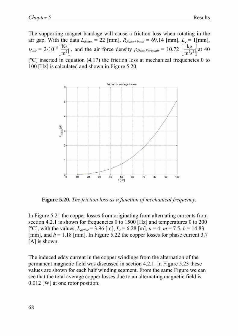
Chapter 5 Results
68
The supporting magnet bandage will cause a friction loss when rotating in the air gap. With the data LRotor = 22 [mm], RRotor+band = 69.14 [mm], Lg = 1[mm],
υ,air = 2 25 Ns
m10− ⎡
⎢⎣ ⎦⋅ ⎤
⎥ , and the air force density ρDens,Force,air = 10.72 2 2kg
m s⎡⎢⎣ ⎦
⎤⎥ at 40
[ºC] inserted in equation (4.17) the friction loss at mechanical frequencies 0 to 100 [Hz] is calculated and shown in Figure 5.20.
Figure 5.20. The friction loss as a function of mechanical frequency.
In Figure 5.21 the copper losses from originating from alternating currents from section 4.2.1 is shown for frequencies 0 to 1500 [Hz] and temperatures 0 to 200 [ºC], with the values, Lactive = 3.96 [m], Lc = 6.28 [m], n = 4, m = 7.5, b = 14.83 [mm], and h = 1.18 [mm]. In Figure 5.22 the copper losses for phase current 3.7 [A] is shown.
The induced eddy current in the copper windings from the alternation of the permanent magnetic field was discussed in section 4.2.1. In Figure 5.23 these values are shown for each half winding segment. From the same Figure we can see that the total average copper losses due to an alternating magnetic field is 0.012 [W] at one rotor position.

Results Chapter 5
69
Irms=27.5 [A]
Irms=15 [A ]
Irms=3.7 [A]
Figure 5.21 The winding (copper) losses originating from alternating currents, 3.7 (lower), 15 (middle), and 27.5 (upper) [A].
Figure 5.22 The winding (copper) losses for phase current 3.7 [A].

Chapter 5 Results
70
Figure 5.23 The winding (copper) losses, from an alternating magnetic field.
Each winding is divided into two halves, covering a half tooth. ωm=235.6 rads
⎡ ⎤⎢ ⎥⎣ ⎦
,
RCu=1.18
2 [mm], Lactive=3.96 [m], and ρRes,Cu=2.25 810−⋅ [Ωm] at 100 [ºC].
Two ball bearings with inner diameter Dm = 30 [mm], friction coefficient µfriction,Bearing = 0.0015, and pre-load torque τ0 = 0.5 [Nm] give rise to bearing friction losses, shown in Figure 5.24.

Results Chapter 5
71
Figure 5.24 The bearing friction losses (two bearings) used in the studied electrical machine as function of mechanical frequency and load torque.
Dm = 30 [mm], τ0 = 0.5 [Nm], µfriction,Bearing= 0.0015.
The average eddy current losses for one magnet is given by
( ) ( )2
, 3 41 2
3 2 2 2
1 12 41 3
2,
1 1, , [W] (5.24)
4 Res PMPM ave PM PM PM
sn h t h
h hh hP h b l B h B hω
ρ ≥ ≥≥ ≥⋅ ⋅
⎛ ⎞⎛ ⎞ ⎛ ⎞⎜ ⎟⎜ ⎟≈ ⋅ ⋅ ⋅ + ⋅⎜ ⎟
⎜ ⎟⎜ ⎟⎜ ⎟⎝ ⎠⎝ ⎠⎝ ⎠⋅ ∑ ∑∑ ∑
By looking at the space losses caused by the fundamental component of the supply inverter current the summations over the harmonic orders are set equal to 1. Now by summing equation (5.24) over all 20 magnets in the studied electrical machine gives:
( ) ( ),
1 31 3
23
1
202 2
, , , ,1 1
[W] (5.25)4PM
Res PMPM ave tot PM PM n h t h
h hi i
s
iP h b l B Bω
ρ ≥ ≥=⋅ ⋅ ⋅
⎛ ⎞⎛ ⎞⎛ ⎞⎜ ⎟⎜ ⎟⎜ ⎟≈ ⋅⎜ ⎟⎜ ⎟ ⎜ ⎟⎝ ⎠ ⎝ ⎠⎝ ⎠
+⋅ ∑ ∑ ∑

Chapter 5 Results
72
In Figure 5.25 the ‘space’ harmonic losses related to the fundamental frequency component of the supply inverter supply is shown. The losses in this Figure are calculated for the fundamental ‘space’ frequency and ‘space’ overtones 2 to 16. The total average permanent magnet losses at one rotor position is 40 [W], also shown in Figure (5.25).
Figure 5.25 The ‘space’ harmonic permanent magnet losses caused by the inverter supply current, related to the fundamental frequency. The losses related
to the space harmonics with the fundamental frequency and overtones 2 to 16 are shown for each magnet. There are 20 magnets in the studied electrical
machine. The excitation RMS current is 3.7 [A]. The magnet dimensions are lPM=7.46 [mm], bPM=16.78 [mm], and hpm= 22 [mm]. The fundamental
frequency of the current is 375 [Hz], ωs=235 rads
⎡ ⎤⎢ ⎥⎣ ⎦
. The resistivity of the
magnet is 64 810−⋅ [Ωm].
If the inverter supply current contains of a component related to the first overtone then the ‘time’ harmonic permanent magnet losses are
( ) ( )20
, 31
23 2
1 1 1 3
2,
1, ,5 [
4PMRes PM
PM ave PM PMs
n h t hi hh ii
P h b l B Bωρ ≥≥=
⋅⎛ ⎞⎛ ⎞ ⎛ ⎞⎜ ⎟⎜ ⎟≈ ⋅ ⋅ ⋅ ⋅ +⎜ ⎟
⎜ ⎟⎜ ⎟⎜ ⎟⎝ ⎠⎝ ⎠⎝ ⎠⋅∑ ∑∑ W] (5.26)

Results Chapter 5
73
The factor 5 in equation (5.26) is related to the harmonic order numbers, from equation (4.36). In this case the fundamental and the first overtone are concerned which means 12+22. Applying equation (5.26) for a current amplitude of 1.5 [A] yields results according to Figure 5.26.
Figure 5.26 The ‘time’ harmonic permanent magnet losses caused by the supply inverter current, related to the first overtone with an amplitude of 1.5 [A RMS]. The losses related to the ‘time’ harmonics with the fundamental ’time’ frequency and overtones 2 to 16 are shown for each magnet. There are 20 magnets in the studied electrical machine. The excitation RMS current is 1.5 [A]. The magnet dimensions are lPM=7.46 [mm], bPM=16.78 [mm], and hpm= 22 [mm]. The first
overtone frequency of the inverter current is 2x375 [Hz], ωs=235 rads
⎡⎢⎣ ⎦
⎤⎥ . The
resistivity of the magnet is 64 810−⋅ [Ωm].
In Figure 5.26 the average total ‘time’ harmonic losses of all permanent magnets are shown for an inverter current related to the first overtone of amplitude of 1.5 [A]. The total ‘time’ harmonic losses related to the first overtone is 19 [W] also shown in the same Figure.
The rest of the ‘time’ harmonic losses are neglected here. As it can be seen from Figure 5.26 the losses are ‘flattened’, i.e. the decrease of the magnetic field components are more than the increase of the square of the ‘time’ harmonic order summations.

Chapter 5 Results
74
The permeance losses occurring at no-load are neglected here, because the studied actuator must produce, during all operation time, at least a small torque that can balance the bearing the losses. Therefore this no-load loss mechanism is not applicable here.
5.3 Simplified Equivalent Circuit Simulation
The simulations done in previous section have paved the way for the simplified equivalent circuit analysis of the actuator systems in a power perspective. The system studied in this work is an aircraft power system containing three actuators, a converter, a generator and passive loads, representing all other power consuming equipments. Each actuator contains of an inverter, electrical machine, and a gear. In Figures 5.29-5.35 examples of output of the simplified circuit simulation model are shown. The efficiency of the gear is set to 0.95 and the inverters to 0.9. The parameters of the electrical machines used in the simulations, shown in the coming Figures, are derived in the previous chapter. In Figure 5.27 a block diagram of the simplified model of a MEA system is shown.
Actuator
Actuator
Actuator
Converter Generator Load
Battery
ESS Load
Inverter
EM
Load
DC/DC
Figure 5.27 The block diagram of the simplified MEA system. Components in standby are dashed.

Results Chapter 5
75
5.3.1 Flight Mission Simulations In the simulation of the simplified power system under a flight mission, load torques are applied to each actuator whereas the angular velocities of the actuators are compared to corresponding reference velocities. The difference between the reference and actual angular velocities are used as inputs to the inverter model after PI-control. This difference signal is used to control the voltage and current of the electrical machines. In Figure 5.28 the implemented components are shown. The inverter is modelled as a transformer with the corresponding resistance efficiency. The electrical machine model is described in Chapter 4. The gear is modelled with an efficiency related to the load torque.
Inverter EM Gear
=
Figure 5.28 The components of the implemented actuator, inverter (left), EM (middle), and gear (right).
The reference load torques and angular velocities are shown in Figure 5.29. The reference angular velocities are made positive, since the electrical machine model is based on RMS-values of voltage. The applied load torque is negative because of the Modelica sign convention. Negative torque means consumption of power while positive sign means generation of power.
The implemented permanent magnet loss has the following form

Chapter 5 Results
76
( )( )
1 31 3
1 31 3
202 2, ,2
1 1 1
,20
2 2, ,
1 1 1
,
1010
n h t hi h him actual actual
PM FEMm FEM
n h t hi h hi i FEM
m rms
iPM
PM FEM
B B
P P
B B
IP
ωω
ω
= ≥ ≥
= ≥ ≥
⎛ ⎞⎛ ⎞⎛ ⎞⎛ ⎞⎜ ⎟⎜ ⎟⎜ ⎟⎜ ⎟⎜ ⎟⎜ ⎟⎜ ⎟ ⎜ ⎟⎜ ⎟⎛ ⎞ ⎝ ⎠ ⎝ ⎠⎝ ⎠⎝ ⎠⎜ ⎟ ⋅ ≈
⎜ ⎟ ⎛ ⎞⎛ ⎞⎛ ⎞⎛ ⎞⎝ ⎠ ⎜ ⎟⎜ ⎟⎜ ⎟⎜ ⎟⎜ ⎟⎜ ⎟⎜ ⎟ ⎜ ⎟⎜ ⎟⎝ ⎠ ⎝ ⎠⎝ ⎠⎝ ⎠
≈
+⋅
≈ ⋅⋅
+
⋅⋅
∑ ∑ ∑
∑ ∑ ∑
( )( ) ( )
( )
2
2
2
,(1)
,(1)
40 193.7 2 37.5
[W] (5.27)m
actual actual
m rms FEM
kI
τ
τω
πω
⎛ ⎞⎛ ⎞ ⎜ ⎟⎜ ⎟⎜ ⎟ ⎝ ⎠= ⋅⎜ ⎟⎜ ⎟⎝ ⎠
+⋅
⋅
⋅ ⋅⋅
where the losses calculated in the previous section by FEM-program are multiplied by a correction factor for taking into account the actual values of the angular frequency and magnetic field density. In equation (5.27) ωm denotes the mechanical angular frequency, Irms,(1) denotes the RMS value of the current related to the fundamental frequency, τ denotes the load torque, and PPM,FEM denotes the total magnet losses calculated by FEM-program in previous section.
In the same way as the correction term for the permanent magnet losses in equation (5.27), a correction term is also introduced for the copper losses due to a rotating magnetic field. The temperature is set to 100 [ºC] for the copper loss calculation and the copper loss from an alternating magnetic field has the following implemented form
( )
2
2, 0.0123.7 2 37.5
[W] (5.28)m
actualCu B
kP τ
τω
π
⎛ ⎞⎜ ⎟⎜ ⎟⎝ ⎠
⋅
⋅=
⋅ ⋅⋅

Results Chapter 5
77
Figure 5.29 The reference load torques (left) and angular velocities (right). Actuator 1 (up), Actuator 2 (middle), Actuator 3 (down).
The response of the electrical machine to the applied torque can be seen in Figures 5.30 and 5.31.

Chapter 5 Results
78
Figure 5.30 The angular velocities (left) and voltages (right) of the electrical machines. Actuator 1 (up), Actuator 2 (middle), Actuator 3 (down).
The angular velocities and voltages of the three actuators are shown in Figure 5.30 respective corresponding torques and currents in Figure 5.31.

Results Chapter 5
79
Figure 5.31 The torques (left) and currents (right) of the electrical machines. Actuator 1 (up), Actuator 2 (middle), Actuator 3 (down)
In Figure 5.32 the losses involved in the electrical machine in the actuator number 1 are shown. The copper and iron losses are the dominating losses as can be seen from Figure 5.32.
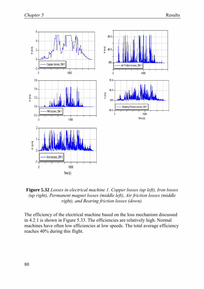
Chapter 5 Results
80
Figure 5.32 Losses in electrical machine 1. Copper losses (up left), Iron losses (up right), Permanent magnet losses (middle left), Air friction losses (middle
right), and Bearing friction losses (down).
The efficiency of the electrical machine based on the loss mechanism discussed in 4.2.1 is shown in Figure 5.33. The efficiencies are relatively high. Normal machines have often low efficiencies at low speeds. The total average efficiency reaches 40% during this flight.

Results Chapter 5
81
Figure 5.33 The efficiency of the electrical machines. Actuator 1 (up), Actuator 2 (middle up), Actuator 3 (middle down), Total average efficiency (down)
The converter is controlled by a PI-regulator, where the output voltage, (i.e. DC-bus) is compared to a 270 V level. The converter is modelled as a fictive transformer with an efficiency of 0.9. In Figure 5.34 the output and input quantities of the converter is shown.

Chapter 5 Results
82
Figure 5.34 The input and output quantities of the converter. Input (left, Output (right), Voltage (up), Current (down).
In Figure 5.35 the average power consumption of the entire flight pass is shown. As expected the average power consumption is relatively low under the entire pass, 60 [W].

Results Chapter 5
83
Figure 5.35 Average power consumption.
In Figure 5.36 the total average current is shown for EM 1. The average value for entire flight is 1.5 [A]. One of the thermal analyses in next chapter is based on this value.
Figure 5.36 Total average phase current for entire flight in EM 1.

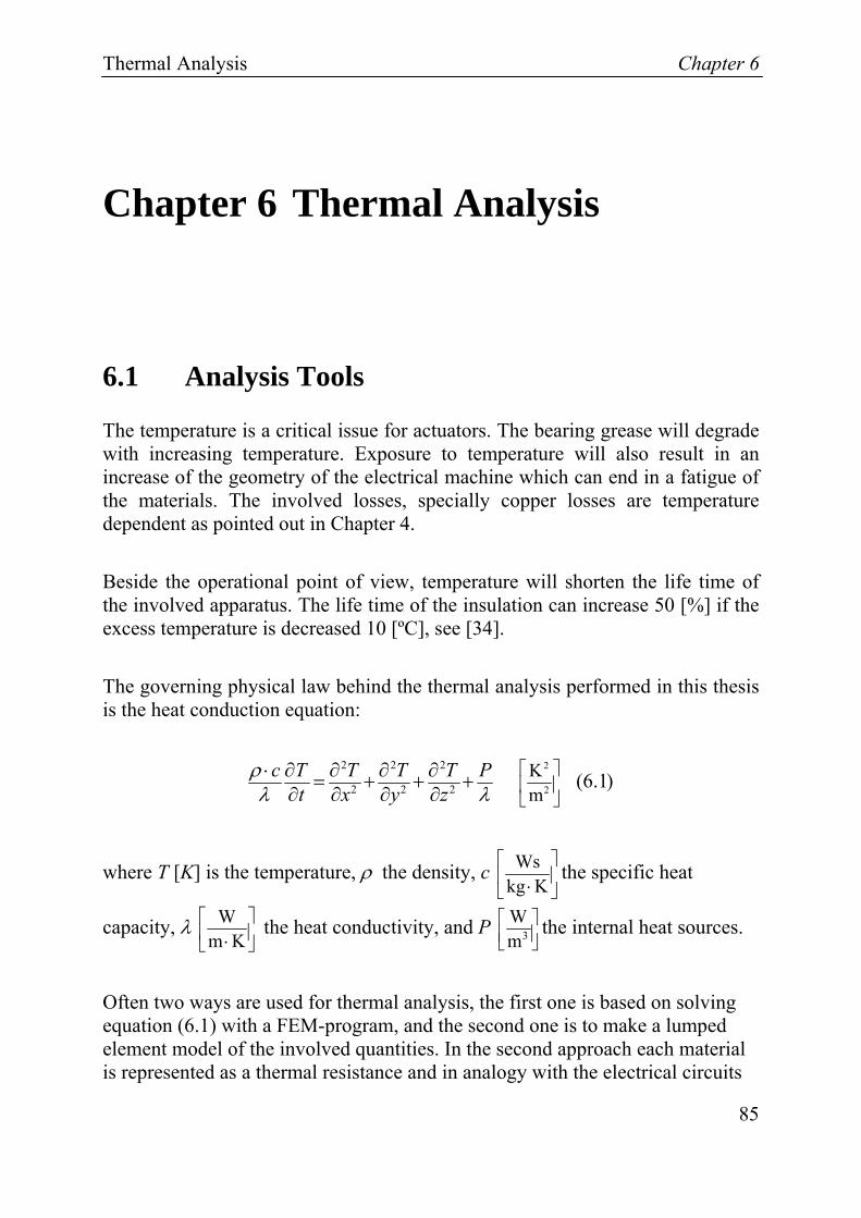
Thermal Analysis Chapter 6
85
Chapter 6 Thermal Analysis
6.1 Analysis Tools
The temperature is a critical issue for actuators. The bearing grease will degrade with increasing temperature. Exposure to temperature will also result in an increase of the geometry of the electrical machine which can end in a fatigue of the materials. The involved losses, specially copper losses are temperature dependent as pointed out in Chapter 4.
Beside the operational point of view, temperature will shorten the life time of the involved apparatus. The life time of the insulation can increase 50 [%] if the excess temperature is decreased 10 [ºC], see [34].
The governing physical law behind the thermal analysis performed in this thesis is the heat conduction equation:
2
2
2 2 2
2 2 2Km
(6.1)c T T T T Pt x y z
ρλ λ
⎡ ⎤⎢ ⎥⎣ ⎦
⋅ ∂ ∂ ∂ ∂= + + +∂ ∂ ∂ ∂
where T [K] is the temperature, ρ the density, c Wskg K⎡ ⎤⎢ ⎥⎣ ⎦⋅
the specific heat
capacity, λ Wm K⎡⎢⎣ ⎦⋅
⎤⎥ the heat conductivity, and P 3
Wm⎡ ⎤⎢ ⎥⎣ ⎦
the internal heat sources.
Often two ways are used for thermal analysis, the first one is based on solving equation (6.1) with a FEM-program, and the second one is to make a lumped element model of the involved quantities. In the second approach each material is represented as a thermal resistance and in analogy with the electrical circuits

Chapter 6 Thermal Analysis
86
there are also heat sources, and capacitances. The heat difference is the across variable and the heat flow the through variable.
In the performed steady state FEM analysis the material thermal properties from Table 6.1 were used. The internal heat sources are the same as mentioned in Chapter 4. In steady state the time derivate of the temperature is set to zero.
Table 6.1 Thermal properties of the involved materials.
Iron Copper PM Air Paper
λ Wm K⎡ ⎤⎢ ⎥⎣ ⎦⋅
40 380 9 0.024 0.09
The boundary conditions are set to 40 [ºC] at the outer radius and 30 [ºC] at the inner boundary. The average values of the loss quantities of the EM 1 from Figure 5.32 in section 5.3.1 were used in the thermal analysis, from Figure 6.1. The average phase RMS current into the EM 1 was 1.5 [A], from Figure 5.36.
Figure 6.1 The temperature distribution in steady state.

Thermal Analysis Chapter 6
87
The loss mechanism involved are, copper, iron, permanent magnet, air, and bearing friction. In Figure 6.1 the steady state heat distribution is shown. The involved losses from 5.3.1 are translated into loss densities, shown in the first row of the Table 6.2. The values on the second row of Table 6.2 are used for another thermal analysis shown in Figure 6.2. These losses are described and calculated in section 5.2.1. The RMS value of the winding current is set to 3.7 [A] at a base velocity of 2250 [rpm].
Table 6.2 Internal heat sources.
Iron Copper PM Air i i
Bearing
P 3
Wm⎡⎢⎣ ⎦
⎤⎥ average 1456 86420 445 17.4 0.19
P 3
Wm⎡⎢⎣ ⎦
⎤⎥ @ 2250 [rpm] 1.1 510⋅ 3-5.5 510⋅ 1.1 610⋅ 1.3 510⋅ 15.4
Copper losses are responsible for 1.5 respective 7.2 [ºC] temperature rise shown in Figures 6.2 and 6.3.
Figure 6.2 The temperature distribution in steady state at 2250 [rpm].


Other Solutions Chapter 7
89
Chapter 7 Other Solutions
7.1 Conventional Hydraulic Actuators
The traditional hydraulic actuators are relatively robust. One of the main advantages of this solution is the high power density related to the hydraulic cylinders. In the cases where accumulators are used, energy can be stored in springs or gas and used easily when needed. In Figure 7.1 an example of controlling surfaces equipped with actuator mechanisms are pointed out.
Figure 7.1 Example of controlled surfaces on an aircraft, from [40]
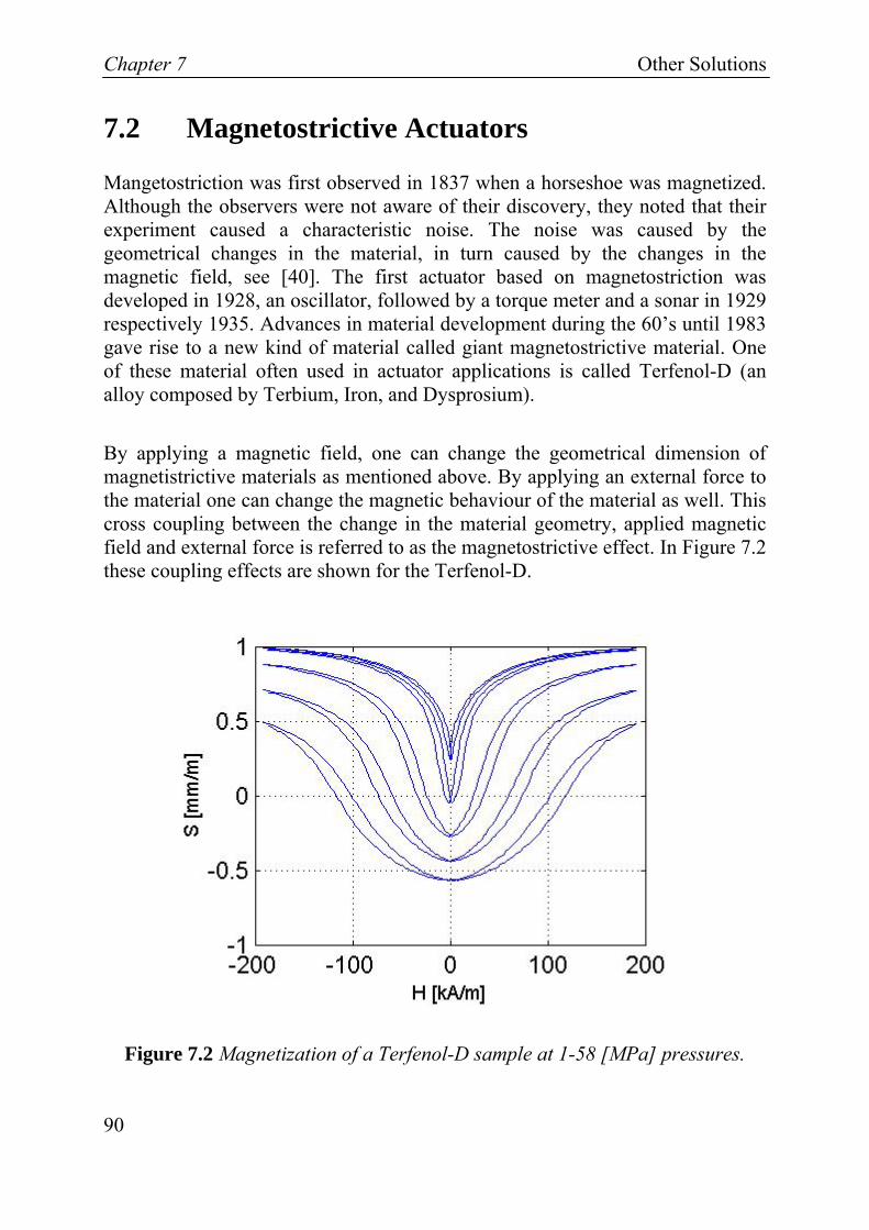
Chapter 7 Other Solutions
90
7.2 Magnetostrictive Actuators
Mangetostriction was first observed in 1837 when a horseshoe was magnetized. Although the observers were not aware of their discovery, they noted that their experiment caused a characteristic noise. The noise was caused by the geometrical changes in the material, in turn caused by the changes in the magnetic field, see [40]. The first actuator based on magnetostriction was developed in 1928, an oscillator, followed by a torque meter and a sonar in 1929 respectively 1935. Advances in material development during the 60’s until 1983 gave rise to a new kind of material called giant magnetostrictive material. One of these material often used in actuator applications is called Terfenol-D (an alloy composed by Terbium, Iron, and Dysprosium).
By applying a magnetic field, one can change the geometrical dimension of magnetistrictive materials as mentioned above. By applying an external force to the material one can change the magnetic behaviour of the material as well. This cross coupling between the change in the material geometry, applied magnetic field and external force is referred to as the magnetostrictive effect. In Figure 7.2 these coupling effects are shown for the Terfenol-D.
Figure 7.2 Magnetization of a Terfenol-D sample at 1-58 [MPa] pressures.

Other Solutions Chapter 7
91
The magnetic field is swept between -200 to 200 kAm
⎡ ⎤⎢ ⎥⎣ ⎦
, while the applied
pressure is 1 to 58 MPa. The measured strain of the Terfenol-D sample, in
Figure 7.2, is close to 1.1 mmm
⎡⎢⎣ ⎦
⎤⎥ for 1 [MPa] and 0.75 mm
m⎡ ⎤⎢ ⎥⎣ ⎦
for 58 [MPa].
The additional physical relations that are often used when modelling the magnetostrictive effect are among others Newton’s second law and Maxwell’s equations. The magnetization curves shown in Figure 7.2 can then be used as material data base.
By placing a couple of Terfenol-D actuators inside an outer stator it is possible to achieve an elliptical motion of this stator. The motion can be controlled by exciting the actuators in appropriate order. Such device was build and analysed in a joint work with Saab AB, see [42]. In this analysis it was shown that it is fully possible to control the elliptical motion of the stator, but the efficiency and the noise level was stated as a considerable weakness of this solution.
Figure 7.3 Example of a ’Magnetostrictive’ actuator, from Saab Dynamic AB, with 12 wounded Terfenol-D actuator rods.

Chapter 7 Other Solutions
92
Figure 7.3 shows the magnetostrictive actuator built by Saab Dynamic AB. The theoretical maximum output power of this device was estimated to 713 [W], maximum torque production to 338 [Nm], and the maximum efficiency to 46 [%].
7.3 Electro-Hydrostatic Actuator
By combining the energy storage capability of a conventional hydraulic system and the power-by-wire principle of the electromechanical system, an Electro-Hydrostatic Actuator is formed. As it was mentioned in Chapter 1 these actuators are not affected to the same extend of the drawbacks of the conventional system. One drawback often related to these actuators is their initial and maintenance cost that is higher than for ‘pure’ electro mechanical actuators.
Figure 7.4 Basic configuration of an EHA, from [43] .
In Figure 7.4 a basic configuration sketch of an electro-hydrostatic actuator is shown, with the components electronic ‘box’, motor, pump, and the hydraulic frame. In Figure 7.5 a block diagram of how such an EHA can be controlled is shown.

Other Solutions Chapter 7
93
Figure 7.5 Control block diagram of an EHA, from [44].
In Figure 7.6 a forerunner to the EHA solution is shown from the aircraft manufacturer Airbus. In this solution a throttle mechanism (i.e. servovalve) is used to control the oil flow.
Figure 7.6 A forerunner to EHA, from [40].
In Figures 7.7 and 7.8 the EHA used in the carrier A380 from Airbus are shown. In these solutions the throttle mechanism is replaced by a pump controlled in its turn by a motor.

Chapter 7 Other Solutions
94
Figure 7.7 An EHA built by Airbus, from [40].
According to the aircraft manufacturer Airbus, the third redundant surface control system is an EHA solution in their new carrier plane A380. By this solution almost 450 [kg] weight reductions is achieved. In Figure 7.6 a 5 [kW] EHA used by Airbus is shown. The total hydraulic power output (conventional plus the EHA actuators) is 500 [kW] in A380 from Airbus.
Figure 7.8 A 5 [kW] EHA solution used in the carrier A380 from the manufacturer Airbus.

Conclusions and Future Work Chapter 8
95
Chapter 8 Conclusions and Future
Work
8.1 Conclusions
In this thesis future MEA actuator systems are discussed. The suggested modelling approach in this thesis facilitates the build-up of a data base of different actuator systems in aircraft that can be used by aircraft dimensioning tools.
The studied electrical machine showed good electromechanical and thermal behaviour. From the flight mission simulations it can be seen that the efficiency of this machine reached 90% relatively fast. The total actuator system average efficiency reached 40 [%], because of the ‘idle’ mode operation of the actuators. The average power consumption was also relatively low. For the entire flight it was 60 [W]. The concentrated winding arrangement in combination with the wide back core, defined in Figure 5.2, and teeth makes the flux paths short. As a result the iron losses will decrease and the upper part of the stator core can be built thinner, resulting in more decrease of the iron losses. The supporting teeth have a cooling effect on the nearest windings, resulting in less copper losses.
A method for calculating the permanent magnet losses caused by the current harmonics and the space harmonics from steady state 2D FEM simulations was suggested. This method is used for calculating the space harmonics from the fundamental component of the inverter current and the time harmonics from the first overtone component of the inverter current. Also a method for calculating the back-EMF constant for concentrated winding arrangement has been derived in this thesis. With this method it is enough to calculate the EMF-constant by 2D FEM steady state calculations. The analytical torque expression was also

Chapter 8 Conclusions and Future Work
96
modified for the studied electrical machine with concentrated windings. Another method was used for the calculation of the magnetic flux density in the iron based on the average value of the fundamental flux density amplitude.
The described concept is considered to offer a cost effective solution for future aircraft actuator systems. The advantages and weaknesses of this solution have also been discussed.
8.2 Future Work
Naturally the equivalent circuit used in the actuator implementation of the simplified model needs to be upgraded regarding the actual number of aircraft power system components. More realistic load data should be used to achieve better agreement between the model and the real situation.
The thermal analysis should be expanded to cover a transient analysis for studies of the start performance of the electrical machines. The steady state temperature study can be attached to the simplified model as suggested in an EHA solution described in [14].
The system models used in this thesis are based on the RMS-values of the electrical quantities. An alternative method is to use average values instead of RMS-values. In this way the sign of the involved quantities is not lost. Alternative models for inverters and converter based on the state and average modelling can be used, see [45].
For comparison and compliance with the major goal of this project a database over the key figures discussed in Chapter 2 is needed, therefore other components (electrical machines, inverter topologies, and gear mechanisms) and other solutions need to be studied in the same manner as done in this thesis.
The possibility of extracting data from FEM-analysis into the Modelica models in parallelized automated processes should be considered since the required number of simulations is relatively high.
Conclusions and Future Work Chapter 8
97
The efficiency of the electronic components should be estimated better. Measurements of the involved losses should be done for verification and improvements of the loss models. The overtones of the inverter currents should be estimated better, specially when studying the permanent magnet losses. Each overtone causes eddy currents in the permanent magnets.

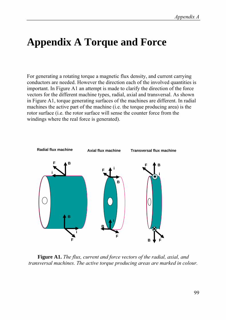
Appendix A
Appendix A Torque and Force
For generating a rotating torque a magnetic flux density, and current carrying conductors are needed. However the direction each of the involved quantities is important. In Figure A1 an attempt is made to clarify the direction of the force vectors for the different machine types, radial, axial and transversal. As shown in Figure A1, torque generating surfaces of the machines are different. In radial machines the active part of the machine (i.e. the torque producing area) is the rotor surface (i.e. the rotor surface will sense the counter force from the windings where the real force is generated).
Radial flux machine Axial flux machine Transversal flux machine
B F
i
B
i
F
F F
F F
B
B
B
B
i i
i
i
Figure A1. The flux, current and force vectors of the radial, axial, and transversal machines. The active torque producing areas are marked in colour.
99

Appendix A
The torque will be produced at the surface directed towards the stator in an axial machine, shown in Figure A1. In the case of the transversal machine the torque is produced at the rotor surface.
100

Appendix B
Appendix B Concentrated or
Distributed Winding
Often in a PM machine the placement of the stator windings are used to categorize these machines. In the traditional electrical machine where the neighbouring windings have different phases is usually referred to as a distributed winding machine. If on the other hand the adjacent winding (i.e. tooth) has the same phase but with a minus sign, is usually referred to as a concentrated winding machine. In Figure B1 examples of such machines are shown.
A
-A
-B
B C’ C
-C
A’
B’ -A’C’
-B’
C’
-A
-B
A-C’ B
-C
C
A’ -A’B’
-B’
(ii) (i)
Figure B1. Principle sketch of 6 phase machines with (i) A distributed winding arrangement. (ii) A concentrated winding arrangement.
101


References
References
[1] M. Torabzadeh-Tari and G. Engdahl: “A Quasi-Static Modelling Approach of Electromechanical Actuators”. The Proceedings of the 2003 International Conference of Magnetism - ICM 2003, Rome, Italy, July 27-1 August, 2003.
[2] M. Torabzadeh-Tari, G. Engdahl, L. Austrin and J. Krah: “A Quasi-Static Modelling Approach Airborne Power Systems”. The 11th National Conference on Machine and Mechanics – NaCoMM 2003, New Dehli, India, December 18-19 2003.
[3] M. Torabzadeh-Tari, G. Engdahl: “A Portable Implementation of a Model of Electromechanical Actuators in More Electric Aircraft Dimensioning Tools”. Actuator 2004, Bremen, Germany, June 14-16 2004.
[4] P.M. Churn, C.J. Maxwell, D Howe, N. Schofield and D.J. Powell: “Electro-Hydraulic Actuation of Primary Flight Control Surfaces”.
[5] G.M. Raimondi, T. Sawata, M. Holme, et al: “Aircraft Embedded Generation Systems”. Power Electronics, Machines and Drives, 16-18 April 2002.
[6] K. Mino, G. Gong and J.W. Kolar: “Novel Hybrid 12-Pulse Line Interphase Transformer Boost-Type Rectifier with Controlled Output Voltage” IEEE
[7] K.W.E. Cheng: “Comparative Study of AC/DC Converters for More Electric Aircraft”. Power Electronics and Variable Speed Drives, 21-23 September 1998.
103
References
[8] D.R. Trainer, C.R. Whitley: “Electric Actuation-Power Quality Management of Aerospace Flight Control systems”. Power Electronics, Machines and Drives, 16-18 April 2002.
[9] D.J. Powell, G.W. Jewell, D. Howe, K. Attalah: “Rotor Topologies for a Switched-Reluctance Machine for the ‘More-Electric’ Aircraft Engine”, IEEE Proceedings, Electrical Power Application, Vol 150 Nob3, May 2003.
[10] T. Skvarenina, P. Krause et al: “Simulation and Analysis of a Switched Reluctance Generator, More Electric Aircraft Power System”, IEEE 1996.
[11] A.J. Mitcham, J.J.A. Cullen: “Permanent Magnet Generator Options for the More Electric Aircraft”, Power Electronics, Machines and Drives, 16-18 April 2002.
[12] http://www.afrlhorizons.com/Briefs/Dec01/PR0103.html
[13] http://www.messier-bugatti.com/company/ index.php4?f=mb_nosenjeux_avionelec
[14] B. Johansson, J. Andersson, P. Krus: ”Thermal Modelling of an Electro-Hydrostatic Actuation System”. Recent Advances in Aerospace Actuation Systems and Components, 13-15 June, Toulouse, France.
[15] G.L. Fronista, G. Bradbury: “ An Electromechanical Actuator for a Transport Aircraft Spoiler Surface”, IEEE
[16] G. Engdahl, L. Austrin et al: “More Electrical Aircraft-Slutrapport” (Swedish), 2000.
[17] http://www.linearmotion.skf.com
[18] P. Kjellqvist: “Modelling and design of electromechanical actuators for active suspension in rail vehicles”, Doctor Thesis, Royal Institute of Technology, TRITA-ETS-2002-03, ISSN-1650-674x, Stockholm, 2002
104

References
[19] N. Ertugrul, W. L. Song, at al: “Investigation of a Fault and High Performance Motor Drive for Critical Applications”, IEEE 2001
[20] http://www.dynasim.se
[21] http://www.modelica.org
[22] F.V. Hunt: “Electroacoustics”, Acoust. Soc. Of America, 1954.
[23] U. Bjurman, G. Engdahl: “Separation of high and low frequency behavior in non-linear circuit simulation, exited with modulated signals”, Transaction on Magnetism, Vol. 36 No4, 2000
[24] E. Hallèn: “Electricitetslära” (Swedish), Stockholm 1953.
[25] G. Bertotti: “Space-Time Correlation Properties of the Magnetization Process and Eddy Current Losses”, Journal of Applied Physics, Vol 55, pp 4339-4355, 1983.
[26] Å. Carlsson: “Power Transformer Design Fundamentals”, Ludvika, 1985.
[27] E. Hallèn, “Electromagnetic Theory”, ISBN 99-0839154-2, London, 1962.
[28] F. Sahin, “Design and Development of a High Speed Axial Flux Permanent Magnet Machine”, Doctor Thesis, Technische Universiteit Eindhoven, The Netherlands, ISBN 90-386-1380-1, 2001.
[29] F. Magnussen ”On Design and Analysis of Synchronous Permanent Magnet Machines for Field-weakening Operation in Hybrid Electric Vehicles”, Doctor Thesis, Royal Institute of Technology, TRITA-ETS-2004-11, ISSN-1650-674x, Stockholm, 2004.
[30] SKF Main Catalogue, (Swedish), Torino,1994.
105

References
[31] J. Engström, “Analysis and Verification of a Slotless Permanent Magnet Motor for High Speed Applications”, Doctor Thesis, Royal Institute of Technology, ISBN 91-7283-130-8, Stockholm,2001
[32] E. Nipp, “Permanent Magnet Motor Drives with Switched Stator Windings”, Doctor Thesis, Royal Institute of Technology, TRITA-EMD-9905, ISSN-1102-0172, Stockholm,1999
[33] G. Engdahl, R. Eriksson, ”Electrotechnical Modeling”, Royal Institute of Technology, A-EEA-0003, Stockholm, 2000.
[34] C. Sadarangani, ”Electrical Machines- Design and Analysis of Induction and Permanent Magnet Motors”, ISBN 91-7170-627-5, Stockholm 2000.
[35] D. K. Cheng, “Field and Wave Electromagnetics”, ISBN 0-201-52820-7, New York, 1989.
[36] C. Bi, Z. Li, S. X. Chen, “Estimation of Back-EMF of PM BLDC Motors Using Derivative of FE Solutions”, IEEE Transaction on Magnetics, Vol 36, No 4, 2000.
[37] P. Thelin, ”Design and Evaluation of a Compact 15 kW PM Integral Motor”, Doctor Thesis, Royal Institute of Technology, TRITA-ETS-2002-02, ISSN-1650-674x, Stockholm, 2002.
[38] F. Libert, ”Design, Optimization and Comparison of Permanent Magnet Motors for a Low-Speed Direct-Driven Mixer”, Licentiate Thesis, Royal Institute of Technology, TRITA-ETS-2004-12, ISSN-1650-674x, Stockholm, 2004.
[39] F. Gustavsson, “Elektriska Maskiner” (Swedish), Stockholm, 1996.
[40] http://www.eads.net/xml/content/OF00000000400004/1/41/559411.pdf
[41] H. Tilberg, “Design in Applied Giant Magnetostriction”, Licentiate Thesis, Royal Institute of Technology, TRITA-EEA-9402, ISSN 1100 1593, Stockholm, 1994.
106

References
[42] L. Qvarnström, “Analysis and Evaluation of a Magnetostrictive Flex Spline Actuator”, Master Thesis, Royal Institute of Technology, Stockholm, 2003.
[43] T.M. Jahns, R.C. Nocker, “Electric Controls for a High-Performance EHA Using an Interior Permanent Magnet Motor Drive”, IEEE 1989.
[44] T. Sadeghi, A. Lyons, “Fault Tolerant EHA Architectures”, IEEE 1992.
[45] G. D. Demetriades ”On Small-Signal Analysis and Control of the Single- and Dual-Active Bridge Totplogies”, Doctor Thesis, Royal Institute of Technology, ISBN-91-7283-966-X, Stockholm, 2005.
[46] P.W. Wheeler et al, “An Electro-Hydrostatic Aircraft Actuator Using Matrix Converter Permanent Magnet Motor Drive”, IEEE 2004.
[47] Data sheet from Data Device Corporation, PWR-82332, 1999,
107


List of Symbols
List of Symbols
Symbol Quantity Unit ϕh Angle [rad] β Angle between current and flux [rad]
ω Angular velocity rads
⎡ ⎤⎢ ⎥⎣ ⎦
ωHigh Angular velocity, high speed side rads
⎡ ⎤⎢ ⎥⎣ ⎦
ωLow Angular velocity, low speed side rads
⎡ ⎤⎢ ⎥⎣ ⎦
ωm Angular velocity, mechanical rads
⎡ ⎤⎢ ⎥⎣ ⎦
ωs Angular frequency , supply rads
⎡ ⎤⎢ ⎥⎣ ⎦
ACu Cross-section area of the conductor, copper [m2]
σ Conductivity of the core material 1Ωm⎡ ⎤⎢ ⎥⎣ ⎦
ξ Conductor height [m] b Conductor width [m] RDC Copper DC-resistance [Ω] kAC Correction factor for AC-losses in copper [ - ] kAC,active Correction factor, active part of the conductor [ - ] kAC,end Correction factor, end part of the conductor [ - ]
ke Counter-EMF constant Vsrad⎡ ⎤⎢ ⎥⎣ ⎦
Reg Couette Reynolds number [ - ] I Current [A] I1 Current [A] I2 Current [A]
J Current density 2
Am⎡ ⎤⎢ ⎥⎣ ⎦
Is,m Current harmonic amplitude [A]
109

List of Symbols
Js,y Line current density in y-direction Am⎡ ⎤⎢ ⎥⎣ ⎦
Irms RMS value of phase current [A]
Jz Axial current density 2
Am⎡ ⎤⎢ ⎥⎣ ⎦
Is,0 Average current [A] is Supply current [A]
ρDens,air Density of air 3
kgm⎡ ⎤⎢ ⎥⎣ ⎦
ρDens,iron Density of core material 3
kgm⎡ ⎤⎢ ⎥⎣ ⎦
ρDens,Force,air Density force of air 3 2
kg mm s⎡ ⎤⎢ ⎥⎣ ⎦
ρdensity Material density 3
kgm⎡ ⎤⎢ ⎥⎣ ⎦
Dm Inner diameter of bearing [m] d0 Effective diameter, screw gear mechanism [mm] η Efficiency [ - ] ηInverter Efficiency of the inverter [ - ] ηEM Efficiency of the electrical machine [ - ] ηGear Efficiency of the gear mechanism [ - ]
E Electric field Vm⎡ ⎤⎢ ⎥⎣ ⎦
kf Empiric constant, core losses [ - ] kh Empiric constant, hysteresis losses [ - ] ke Empiric constant, Excess losses [ - ] W Magnetic energy [J] ψΘ Flux linkage at angle Θ [Vs] ψ Flux linkage [Vs] ϕ Flux [Wb] fe Frequency, electrical [Hz] Cf Friction coefficient [ - ] μfriction,Bearing Friction coefficient [ - ] μfri,Gear Friction coefficient [ - ] F Force [N] Fs Force along [N] h1 Harmonic order [ - ] h2 Harmonic order [ - ] h3 Harmonic order [ - ] h4 Harmonic order [ - ]
110

List of Symbols
ϕs,h Phase of the current [rad] Ze Impedance, electrical [Ω] Zm Impedance, mechanical [Ω] Ltot Total inductance [H] Ld d-inductance [H] Lq q-inductance [H]
Ph Lead of spindle mmrev
⎡ ⎤⎢ ⎥⎣ ⎦
lCu Length of the conductor, copper [m] Lactive Length of the winding, active part [m] Lc Length of the winding, total [m] bPM Length of the permanent magnet [m] lPM Height of the permanent magnet [m] hPM Axial length of the permanent magnet [m] LRotor Axial length of the rotor [m] Lg Air gap length [m] LRotor Length of he rotor [m] BBave Average magnetic flux density [T] BBm Magnetic flux density in iron [T] BB(1),airgap Airgap magnetic flux density [T] BBairgap Magnetic flux density in air gap [T] BBR Magnetic radial flux density in air gap [T] BBϕ Magnetic angular flux density in air gap [T] BBn Magnetic normal flux density in air gap [T] BBt Magnetic tangential flux density in air gap [T] BBleak,n Magnetic flux density, normal component [T] BBleak,t Magnetic flux density, tangential component [T] BBh Magnetic flux density, Fourier series coefficient, [T] BBh,n,PM Magnetic flux density, Fourier series coefficient [T] BBh,t,PM Magnetic flux density, Fourier series coefficient [T] B Magnetic flux density [T] BBz Axial magnetic flux density [T]
H Magnetic field intensity Am⎡ ⎤⎢ ⎥⎣ ⎦
Hz Axial magnetic intensity Am⎡ ⎤⎢ ⎥⎣ ⎦
Hc Coercive magnetic intensity Am⎡ ⎤⎢ ⎥⎣ ⎦
M Magnetization density Am⎡ ⎤⎢ ⎥⎣ ⎦
111

List of Symbols
Mz Axial magnetization density Am⎡ ⎤⎢ ⎥⎣ ⎦
A Magnetic vector potential Wbm
⎡ ⎤⎢ ⎥⎣ ⎦
A2 Magnetic vector potential Wbm
⎡ ⎤⎢ ⎥⎣ ⎦
AΘ Magnetic vector potential Wbm
⎡ ⎤⎢ ⎥⎣ ⎦
A1 Magnetic vector potential Wbm
⎡ ⎤⎢ ⎥⎣ ⎦
JInertia Moment of inertia 2Nms
rad⎡ ⎤⎢ ⎥⎣ ⎦
m Number of conductor layers, winding [ - ] n Number of conductor per layer [ - ] Nph Number of phases [ - ] N Number of turns per slot (half tooth) [ - ] K Number of teeth [ - ] Q Number of slots [ - ] r1 Peripheral radius [m] r2 Peripheral radius [m] α1 Phase shift [rad] α3 Phase shift [rad] Pfriction,air Power losses, air friction [W] Piron Power losses, iron [W] PB,Cu Power losses, copper, per tooth per conductor [W] PB,Cu,ave Power losses, average copper losses per tooth [W] Ptot,B,Cu Power losses, total average copper losses [W] PCU Power losses, copper [W] PPM Permanent magnet losses [W]
PPM,Dens,,ave Average permanent magnet power loss density 3
Wm⎡ ⎤⎢ ⎥⎣ ⎦
Pfriction,bearing Bearing friction losses [W] RCu Radius of the copper [m] RRotor Radius of the rotor [m] μr Relative permeability [ - ] ρRes,Cu Resistivity of copper [ ]mΩ Ron Resistance, conduction [ ]Ω ρresistivity Material resistivity [ ]mΩ ρRes,PM Resistivity of permanent magnet [ ]mΩ
112
List of Symbols
a Slot width [m]
v Speed ms
⎡ ⎤⎢ ⎥⎣ ⎦
TCU Temperature of the copper [ºC] wlamination Thickness of the core lamination [m] t Time [s]
Tem Transduction coefficient Vsm
⎡ ⎤⎢ ⎥⎣ ⎦
= NA⎡ ⎤⎢ ⎥⎣ ⎦
Tme Transduction coefficient NA⎡ ⎤⎢ ⎥⎣ ⎦
= Vsm
⎡ ⎤⎢ ⎥⎣ ⎦
τ Torque [Nm] τave Average torque [Nm]
kτ Torque constant NmA
⎡ ⎤⎢ ⎥⎣ ⎦
τHigh Torque, high speed side [Nm] τL Torque, load [Nm] τLow Torque, low speed side [Nm] τ0 Torque, pre-load [Nm] µ0 Vacuum permeability [ - ] νair Kinematic viscosity [ - ] U Voltage [V] VDC DC-bus Voltage [V] e Induced volatge [V] VCu Volume of copper [m3] Vrms RMS value of voltage [V] Vdiode,drop Voltage drop over the diodes [V] kwindFactor Winding factor [ - ] W Virtual work [J]
113


Index
Index
ABB...............................................29 Actuator ............................. 4,7,89-92 Angular velocity ....................8,27,30 Bearing ..........................................42 Coercive....................................14,44 Cogging .........................................56 Concentrated..................................62 Conventional ..............................7,89 Cooling ............................................9 Copper ......................................33,34 Current............................30,39,43,61 Dirac ..............................................10 dq-coordinates ...............................19 Dymola ..........................................29 Eddy current ........................33,39,68 Efficiency ...............3,11,26,31,32,92 EHA................................... 3,9,92-94 Electric brake...................................4 Electric field ..................................41 Electrical machine ................ 9,13-22 EM ....................................5,10,13,83 EMA .........................3,5,10,13,27,45 EMF.............................5,29,30,61,95 Energy ...........................................63 Farraday.........................................56 FEM..................................5,29,47,95 Flux linkage..............................56,58 Force ....................................14,53,54 Frequency ..............................8,32,33 Friction ...........................32,37,68,71 Gear .......................................4,26,32 H-bridge.........................................24 Hydraulic ....................................3,87 Impedance .....................................30
Inductance ..................................... 63 Inertia ............................................ 31 Inverter ..................................... 24,32 Iron ...................................... 32,33,64 Kirchhoff ....................................... 31 Load............................................... 31 Lorentz .......................................... 53 Loss ............................... 32-42,64-73 Magnetic flux ..................................33,56-58 flux density.......35,39,42,51,65-67 vector potential................51,57-59 Machine............................................. Asynchronous............................ 14 Axial flux ............................. 21,22 DC ........................................ 14,15 Indution ..................................... 16 Permanent magnet ..........14,18-20 Radial ........................................ 19 Reluctance.......................14,16,17 Synchronous......................... 14,17 Transversal ........................... 22,23 Magnetostrictive.................... 7,90,91 Maintenance ............................... 7,14 Maxwell......................................... 91 MEA......................1,3,7,10,27,74,95 Methods......................................... 29 Park transformation....................... 19 Permanent magnet.....18-23,38,42,72 Power.................................. 4,9,11,14 Power density........................ 4,11,14 PWM ............................................. 23 Quasi-static...................................... 4 Reliability...................................... 14
115

Index
Reynolds number...........................38 Rotor ..............................................15 SAAB .......................................48,91 Short circuit ...................................14 SKF................................................26 SPAB ........................................47,48 Temperature....................11,14,34,85 Thermal.......................................5,85 Torque................8,17,27,54,61,62,99 Transduction..................................30 voltage ......................................30,56 vulnerability.....................................7 UAV ................................................7 Unmanned airborne vehicle ............7
116