analysis of laterally loaded long or
DESCRIPTION
Analysis of Laterally Loaded Long OrTRANSCRIPT

Analysis of Laterally Loaded Long or Intermediate Drilled Shafts of Small or Large Diameter in Layered Soil Final Report
Report CA04-0252 December 2008
Division of Research & Innovation
Analysis of Laterally Loaded Long or Intermediate Drilled Shafts of Small or Large Diameter in Layered Soils
Final Report
Report No. CA04-0252
December 2008
Prepared By:
Department of Civil and Environmental Engineering
University of Nevada, Reno Reno, NV 89557
Prepared For:
California Department of Transportation Engineering Services Center
1801 30th Street Sacramento, CA 95816
California Department of Transportation Division of Research and Innovation, MS-83
1227 O Street Sacramento, CA 95814

DISCLAIMER STATEMENT
This document is disseminated in the interest of information exchange. The contents of this report reflect the views of the authors who are responsible for the facts and accuracy of the data presented herein. The contents do not necessarily reflect the official views or policies of the State of California or the Federal Highway Administration. This publication does not constitute a standard, specification or regulation. This report does not constitute an endorsement by the Department of any product described herein.

STATE OF CALIFORNIA DEPARTMENT OF TRANSPORTATION TECHNICAL REPORT DOCUMENTATION PAGE TR0003 (REV. 10/98)
1. REPORT NUMBER
CA04-0252
2. GOVERNMENT ASSOCIATION NUMBER
3. RECIPIENT’S CATALOG NUMBER
4. TITLE AND SUBTITLE Analysis of Laterally Loaded Long or Intermediate Drilled Shafts of Small or Large Diameter in Layered Soil
5. REPORT DATE
December, 2008 6. PERFORMING ORGANIZATION CODE
7. AUTHOR(S) Mohamed Ashour, Gary Norris, Sherif Elfass
8. PERFORMING ORGANIZATION REPORT NO.
UNR / CCEER 01-02
9. PERFORMING ORGANIZATION NAME AND ADDRESS
Department of Civil & Environmental Engineering University of Nevada Reno, NV 89557-0152
10. WORK UNIT NUMBER
11. CONTRACT OR GRANT NUMBER
DRI Research Task No. 0252 Contract No. 59A0348
12. SPONSORING AGENCY AND ADDRESS
California Department of Transportation Engineering Services Center 1801 30th Street Sacramento, CA 95816 California Department of Transportation Division of Research and Innovation, MS-83 1227 O Street Sacramento, CA 95814
13. TYPE OF REPORT AND PERIOD COVERED
Final Report
14. SPONSORING AGENCY CODE
913
15. SUPPLEMENTAL NOTES
This report may also be referenced as report UNR / CCEER 01-02 published by the University of Nevada, Reno.
16. ABSTRACT
Strain wedge (SW) model formulation has been used, in previous work, to evaluate the response of a single pile or a group of piles (including its pile cap) in layered soils to lateral loading. The SW model approach provides appropriate prediction for the behavior of an isolated pile and pile group under lateral static loading in layered soil (sand and/or clay). The SW model analysis covers the entire range of soil strain or pile deflection that may be encountered in practice. The method allows development of p-y curves for the single pile based on soil-pile interaction by considering the effect of both soil and pile properties (i.e. pile size, shape, bending stiffness, and pile head fixity condition) on the nature of the p-y curve. This study has extended the capability of the SW model in order to predict the response of laterally loaded large diameter shafts considering 1) the influence of shaft type (long, intermediate or short) on the lateral shaft response; 2) the nonlinear behavior of shaft material (steel and/or concrete) and its effect on the soil-shaft-interaction; 3) developing (partial or complete) liquefaction in the surrounding soil profile based on far and near-field induced pore water pressure; and 4) vertical side shear resistance along the shaft wall that has a significant contribution to the lateral shaft response. The incorporation of the nonlinear behavior of shaft material, soil liquefaction and vertical side shear resistance has a significant influence on the nature of the calculated p-y curves and the associated t-z curves. Contrary to the traditional Matlock-Reese p-y curve that was established for small diameter long (slender) piles and does not account for soil liquefaction and the variation in the shaft bending stiffness, the current approach for large diameter shafts can provide the p-y curve based on varying liquefaction conditions, vertical and horizontal shear resistance along the shaft, and the degradation in shaft flexural stiffness. In addition, the technique presented allows the classification and the analysis of the shaft as long, intermediate or short based on soil-shaft interaction.
17. KEY WORDS
Laterally Loaded Deep Foundations, Drilled Shafts, Strain Wedge Model, Layered Soils, Nonlinear Behavior of Shaft Material, Liquefaction, Vertical Side Shear
18. DISTRIBUTION STATEMENT No restrictions. This document is available to the public through the National Technical Information Service, Springfield, VA 22161
19. SECURITY CLASSIFICATION (of this report)
Unclassified
20. NUMBER OF PAGES 219 Pages
21. PRICE
Reproduction of completed page authorized

ANALYSIS OF LATERALLY LOADED LONG OR INTERMEDIATEDRILLED SHAFTS OF SMALL OR LARGE
DIAMETER IN LAYERED SOIL
(FINAL)
CCEER 01-02
Prepared by:
Mohamed Ashour Research Assistant Professor
Gary NorrisProfessor of Civil Engineering
and
Sherif ElfassResearch Assistant Professor
University of Nevada, RenoDepartment of Civil Engineering
Prepared for:
State of CaliforniaDepartment of Transportation
Contract No. 59A0348
June 2004

i
ACKNOWLEDGMENTS
The authors would like to thank Caltrans for its financial support of this project. The authors would also
like to acknowledge Dr. Saad El-Azazy, Mr. Anoosh Shamsabadi, Dr. Abbas Abghari, Mr. Angel
Perez-Copo, Mr Steve McBride, Mr. Bob Tanaka and Mr. Tom Schatz for their support and guidance
as the Caltrans monitors for this project.

ii
DISCLAIMER
The contents of this report reflect the views of the authors who are responsible for the facts and
accuracy of the data presented herein. The contents do not necessarily reflect the official views or
policies of the State of California or the Federal Highway Administration. This report does not
constitute standard specifications, or regulations.

iii
ABSTRACT
Strain wedge (SW) model formulation has been used, in previous work, to evaluate the response of a single
pile or a group of piles (including its pile cap) in layered soils to lateral loading. The SW model approach
provides appropriate prediction for the behavior of an isolated pile and pile group under lateral static loading
in layered soil (sand and/or clay). The SW model analysis covers the entire range of soil strain or pile
deflection that may be encountered in practice. The method allows development of p-y curves for the single
pile based on soil-pile interaction by considering the effect of both soil and pile properties (i.e. pile size,
shape, bending stiffness, and pile head fixity condition) on the nature of the p-y curve.
This study has extended the capability of the SW model in order to predict the response of laterally loaded
large diameter shafts considering 1) the influence of shaft type (long, intermediate or short) on the lateral
shaft response; 2) the nonlinear behavior of shaft material (steel and/or concrete) and its effect on the soil-
shaft-interaction; 3) developing (partial or complete) liquefaction in the surrounding soil profile based on far-
and near-field induced porewater pressure; and 4) vertical side shear resistance along the shaft wall that has
a significant contribution to the lateral shaft response.
The incorporation of the nonlinear behavior of shaft material, soil liquefaction and vertical side shear
resistance has a significant influence on the nature of the calculated p-y curves and the associated t-z curves.
Contrary to the traditional Matlock-Reese p-y curve that was established for small diameter long (slender)
piles and does not account for soil liquefaction and the variation in the shaft bending stiffness, the current
approach for large diameter shafts can provide the p-y curve based on varying liquefaction conditions,
vertical and horizontal shear resistance along the shaft, and the degradation in shaft flexural stiffness. In
addition, the technique presented allows the classification and the analysis of the shaft as long, intermediate
or short based on soil-shaft interaction.

iv
TABLE OF CONTENTS
CHAPTER 1
INTRODUCTION....................................................................................................1-1
CHAPTER 2
SHAFT CLASSIFIFACTION AND CHARACTRIZATION ............................2-1
2.1 SHAFT CLASSIFICATION..........................................................................2-1
2.2 FOUNDATION STIFFNESS MODELING..................................................2-2
2.3 LARGE DIAMETER SHAFT.......................................................................2-2
CHAPTER 3
VERTICAL SIDE SHEAR AND TIP RESIATNCES OF
LARGE DIAMTER SHAFTS IN CLAY...............................................................3-1
3.1 INTRODUCTION .........................................................................................3-1
3.2 LOAD TRANSFER AND PILE SETTLEMENT.........................................3-2
3.3 DEVELOPED t-z CURVE RELATIONSHIP ..............................................3-5
3.3.1 Ramberg-Osgood Model for Clay......................................................3-7
3.4 PILE TIP (SHAFT BASE) RESISTANCE IN CLAY..................................3-8
3.5 PROCEDURE VALIDATION......................................................................3-9
3.5.1 Comparison with the Seed-Reese t-z Curve in
Soft Clay (California Test).................................................................3-9
3.6 SUMMARY...................................................................................................3-11
CHAPTER 4
VERTICAL SIDE SHEAR AND TIP RESIATNCES OF
LARGE DIAMTER SHAFTS IN SAND ...............................................................4-1
4.1 INTRODUCTION .........................................................................................4-1
4.2 PILE TIP (SHAFT BASE) RESISTANCE AND .........................................
SETTLEMENT (QT – zT) IN SAND.............................................................4-1

v
4.2.1 Pile Tip Settlement.............................................................................4-5
4.3 LOAD TRANSFER ALONG THE PILE/SHAFT
SIDE (VERTICAL SIDE SHEAR)................................................................4-6
4.3.1 Method of Slices for Calculating the Shear Deformation
and Vertical Displacement in Cohesionless Soil................................4-6
4.3.2 Ramberg-Osgood Model for Sand .....................................................4-11
4.3.3 Procedure Steps to Assess Load Transfer and Pile
Settlement in Sand (t-z Curve)...........................................................4-12
4.4 PROCEDURE VALIDATION......................................................................4-15
4.5 SUMMARY...................................................................................................4-16
CHAPTER 5
MODELING LATERALLY LOADED LARGE DIAMTER
SHAFTS USING THE SW MODEL......................................................................5-1
5.1 INTRODUCTION .........................................................................................5-1
5.2 THE THEORETICAL BASIS OF STRAIN
WEDGE MODEL CHARACTERIZATION.................................................5-2
5.3 SOIL PASSIVE WEDGE CONFIGURATION ............................................5-3
5.4 STRAIN WEDGE MODEL IN LAYERED SOIL........................................5-5
5.5 SOIL STRESS-STRAIN RELATIONSHIP ..................................................5-7
5.5.1 Horizontal Stress Level (SL)..............................................................5-9
5.6 SHEAR STRESS ALONG THE PILE SIDES (SLt).....................................5-11
5.6.1 Pile Side Shear in Sand ......................................................................5-11
5.6.2 Pile Side Shear Stress in Clay............................................................5-11
5.7 SOIL PROPERTY CHARACTERIZATION IN
THE STRAIN WEDGE MODEL..................................................................5-12
5.7.1 Properties Employed for Sand Soil ....................................................5-13
5.7.2 The Properties Employed for Normally Consolidated Clay..............5-14
5.8 SOIL-PILE INTERACTION IN THE STRAIN WEDGE MODEL.............5-16
5.9 PILE HEAD DEFLECTION .........................................................................5-19
5.10 ULTIMATE RESISTANCE CRITERIA IN

vi
STRAIN WEDGE MODEL...........................................................................5-20
5.10.1 Ultimate Resistance Criterion of Sand Soil........................................5-20
5.10.2 Ultimate Resistance Criterion of Clay Soil........................................5-21
5.11 VERTICAL SIDE SHEAR RESISTANCE ..................................................5-22
5.12 SHAFT BASE RESISTANCE ......................................................................5-22
5.13 STABILITY ANALYSIS IN THE STRAIN WEDGE MODEL ..................5-24
5.13.1 Local Stability of a Soil Sublayer in the Strain Wedge Model..........5-24
5.13.2 Global Stability in the Strain Wedge Model......................................5-24
5.14 SUMMARY...................................................................................................5-25
CHAPTER 6
SHAFTS IN LIQUEFIABLE SOILS .....................................................................6-1
6.1 INTRODUCTION .........................................................................................6-1
6.2 METHOD OF ANALYSIS............................................................................6-3
6.2.1 Free-Field Excess Pore Water Pressure, uxs, ff ...............................................6-4
6.2.2 Near-Field Excess Pore Water Pressure , uxs, nf ..............................6-5
6.3 CASE STUDIES ............................................................................................6-12
6.3.1 Post-Liquefaction Response of Completely
Liquefied Nevada Sand ......................................................................6-12
6.3.2 Post-Liquefaction Response of Completely
Liquefied Ione Sand ...........................................................................6-13
6.3.3 Post-liquefaction Response of Partially and Completely
Liquefied Fraser River Sand ..............................................................6-13
6.4 UNDRAINED STRAIN WEDGE MODEL FOR LIQUEFIED SAND.......6-13
6.5 SOIL-PILE INTERACTION IN THE SW MODEL UNDER
UNDRAINED CONDITIONS ......................................................................6-16
6.6 SUMMARY...................................................................................................6-17
CHAPTER 7
FAILURE CRITERIA OF SHAFT MATERIALS ..............................................7-1
7.1 INTRODUCTION .........................................................................................7-1

vii
7.2 COMBINATION OF MATERIAL MODELING WITH
THE STRAIN WEDGE MODEL..................................................................7-3
7.2.1 Material Modeling of Concrete Strength and Failure Criteria ...........7-4
7.2.2 Material Modeling of Steel Strength..................................................7-7
7.3 MOMENT-CURVATURE (M-Φ) RELATIONSHIP...................................7-9
7.4 ANALYSIS PROCEDURE ...........................................................................7-10
7.4.1 Steel Shaft ..........................................................................................7-10
7.4.2 Reinforced Concrete Shaft .................................................................7-15
7.4.3 Concrete Shaft with Steel Case (Cast in Steel Shell, CISS)...............7-18
7.4.4 Reinforced Concrete Shaft with Steel Case
(Cast in Steel Shell, CISS) .................................................................7-20
7.5 SUMMARY .........................................................................7-21
CHAPTER 8
VERIFICATIONS WITH FIELD LOAD TESTS ................................................8-1
8.1 INPUT DATA................................................................................................8-1
8.1.1 Shaft Properties..................................................................................8-1
8.1.2 Soil Properties....................................................................................8-1
8.1.3 Liquefaction analysis (for saturated sand) .........................................8-2
8.1.4 Loads (shear force, moment and axial load)......................................8-2
8.1.5 Earthquake Excitation (Liquefaction) ................................................8-2
8.2 LAS VEGAS FIELD TEST (SHORT SHAFT).............................................8-3
8.3 SOUTHERN CALIFORNIA FIELD TEST (SHORT SHAFT)....................8-5
8.4 TREASURE ISLAND FULL-SCALE LOAD TEST
ON PILE IN LIQUEFIED SOIL ............................................................8-6
8.5 COOPER RIVER BRIDGE TEST AT THE MOUNT
PLEASANT SITE, SOUTH CAROLINA SITE............................................8-8
8.6 UNIVERSITY OF CALIFORNIA, LOS ANGELES (UCLA)
FULL-SCALE LOAD TEST ON LARGE DIAMETER SHAFT.................8-11
8.7 FULL-SCALE LOAD TEST ON A BORED PILE IN LAYERED
SAND AND CLAY SOIL..............................................................................8-13
viii
8.8 SUMMARY...................................................................................................8-13
APPENDIX I
REFERENCES

1-1
CHAPTER 1
INTRODUCTION
The problem of a laterally loaded large diameter shafts has been under investigation and
research for the last decade. At present, the p-y method developed by Matlock (1970)
and Reese (1977) for slender piles is the most commonly used procedure for the analysis
of laterally loaded piles/shafts. The confidence in this method is derived from the fact
that the p-y curves employed have been obtained (back calculated) from a few full-scale
field tests. Many researchers since have attempted to improve the performance of the p-y
method by evaluating the p-y curve based on the results of the pressuremeter test or
dilatometer test.
The main drawback with the p-y approach is that p-y curves are not unique. Instead the p-
y relationships for a given soil can be significantly influenced by pile properties and soil
continuity and are not properly considered in the p-y approach. In addition, the p-y curve
has been used with large diameter long/intermediate/short shafts, which is a compromise.
The SW model proposed by Norris (1986) analyzes the response of laterally loaded piles
based on a representative soil-pile interaction that incorporates pile and soil properties
(Ashour et al. 1998). The SW model does not require p-y curves as input but instead
predicts the p-y curve at any point along the deflected part of the loaded pile using a
laterally loaded soil-pile interaction model. The effect of pile properties and surrounding
soil profile on the nature of the p-y curve has been presented by Ashour and Norris
(2000). However, the current SW model still lack the incorporation of the vertical side
shear resistance that has growing effect on the lateral response of large diameter
piles/shafts. In addition, many of the large diameter shafts could be designed as long
shafts and in reality they behave as intermediate shafts. Compared to the long shaft
characteristics, the intermediate shaft should maintain softer response. It is customary to
use the traditional p-y curves for the analysis of all types of piles/shafts
(short/intermediate/long) which carries significant comprise.

1-2
The lateral response of piles/shafts in liquefied soil using the p-y method is based on the
use of traditional p-y curve shape for soft clay corresponding to the undrained residual
strength (Sr) of liquefied sand. Typically Sr is estimated using the standard penetration
test (SPT) corrected blowcount, (N1)60, versus residual strength developed by Seed and
Harder (1990). For a given (N1)60 value, the estimated values of Sr associated with the
lower and upper bounds of this relationship vary considerably. Even if a reasonable
estimate of Sr is made, the use of Sr with the clay curve shape does not correctly reflect
the level of strain in a liquefied dilative sandy material. The p-y relationship for a
liquefied soil should be representative of a realistic undrained stress-strain relationship of
the soil in the soil-pile interaction model for developing or liquefied soil. Because the
traditional p-y curve approach is based on static field load tests, it has been adapted to the
liquefaction condition by using the soft clay p-y shapes with liquefied sand strength
values.
In the last several years, the SW model has been improved and modified through a
number of research phases with Caltrans to accommodate:
• a laterally loaded pile with different head conditions that is embedded in multiple soil
layers (report to Caltrans, Ashour et al. 1996)
• nonlinear modeling of pile materials (report to Caltrans, Ashour and Norris 2001);
• pile in liquefiable soil (report to Caltrans, Ashour and Norris 2000); and
• pile group with or without cap (report to Caltrans, Ashour and Norris 1999)
The current report focuses on the analysis of large diameter shafts under lateral loading
and the additional influential parameters, such as vertical side shear resistance, compared
to piles. It also addresses the case of complete liquefaction and how the completely
liquefied soil rebuilds significant resistance due to its dilative nature after losing its whole
strength. The assessment of the t-z curve along the length of shaft and its effect on the
shaft lateral response is one of the contributions addressed in this report
1-3
The classification of the shaft type whether it behaves as short, intermediate or long shaft
has a crucial effect on the analysis implemented. The mechanism of shaft deformation
and soil reaction is governed by shaft type (geometry, stiffness and head conditions) as
presented in Chapter 2.
The assessment of the vertical side shear due to the shaft vertical movement induced by
either axial or lateral loading is presented in Chapter 3 and 4. New approach for the
prediction of the t-z curve in sand and clay is also presented. Since the lateral resistance
of the shaft base has growing effect on the short/intermediate shaft lateral response, a
methodology to evaluate the shaft base resistance in clay/sand is also presented in
Chapters 3 and 4.
The SW model relates one-dimensional BEF analysis (p-y response) to a three-
dimensional soil pile interaction response. Because of this relation, the SW model is also
capable of determining the maximum moment and developing p-y curves for a pile under
consideration since the pile load and deflection at any depth along the pile can be
determined. The SW model has been upgraded to deal with short, intermediate and long
shafts using varying mechanism. The degradation in pile/shaft bending stiffness and the
effect of vertical side shear resistance are also integrated in the assessed p-y curve. A
detailed summary of the theory incorporated into the SW model is presented in Chapter
5.
Soil (complete and partial) liquefaction and the variation in soil resistance around the
shaft due to the lateral load from the superstructure are presented in Chapter 6. Based on
the results obtained from the Treasure Island field test (sponsored by Caltrans), it is
obvious that none of the current techniques used to analyze piles/shafts in liquefied soils
reflects the actual behavior of shafts under developing liquefaction. New approach is
presented in Chapter 6 to assess the behavior of liquefied soil and will be incorporated in
the SW model analysis as seen in Chapter 8.
1-4
The nonlinear behavior of shaft material (steel and concrete) is a major issue in the
analysis of large diameter shafts. Such nonlinear behavior of shaft material should be
reflected on the nature of the p-y curve and the formation of a plastic hinge as presented
in Chapter 7.
Several case studies are presented in this study to exhibit the capability of the SW model
and how the shaft classification, shaft material modeling (steel and/or concrete) and soil
liquefaction can be all implemented in the SW model analysis. Comparisons with field
results and other techniques also are presented in Chapter 8.

2-1
CHAPTER 2
CLASSIFICATION AND CHARACTERIZATION OF
LARGE DIAMETER SHAFTS
2.1 SHAFT CLASSIFICATION
The lateral load analysis procedures differ for short, intermediate and long shafts. The short,
intermediate and long shaft classifications are based on shaft properties (i.e. length, diameter and
bending stiffness) and the soil conditions described as follows. A shaft is considered “short” so
long as it maintains a lateral deflection pattern close to a straight line. A shaft classified as
“intermediate” under a given combination of applied loads and soil conditions may respond as a
“short” shaft for the same soil profile for a different combination of applied loads and degraded
soil properties (e. g. a result of soil liquefaction).
The shaft is defined as “long” when L/T / 4. L is the shaft length below ground surface and T
is the relative stiffness defined as T = (EI/f)0.2 where f is the coefficient of subgrade reaction
(F/L3). The computer Shaft treats the given shaft as a short shaft. The value of relative stiffness,
T, varies with EI and f. For a short shaft, the bending stiffness (EI) in the analysis could have a
fixed value (linear elastic). The coefficient of subgrade reaction, f, varies with level of deflection
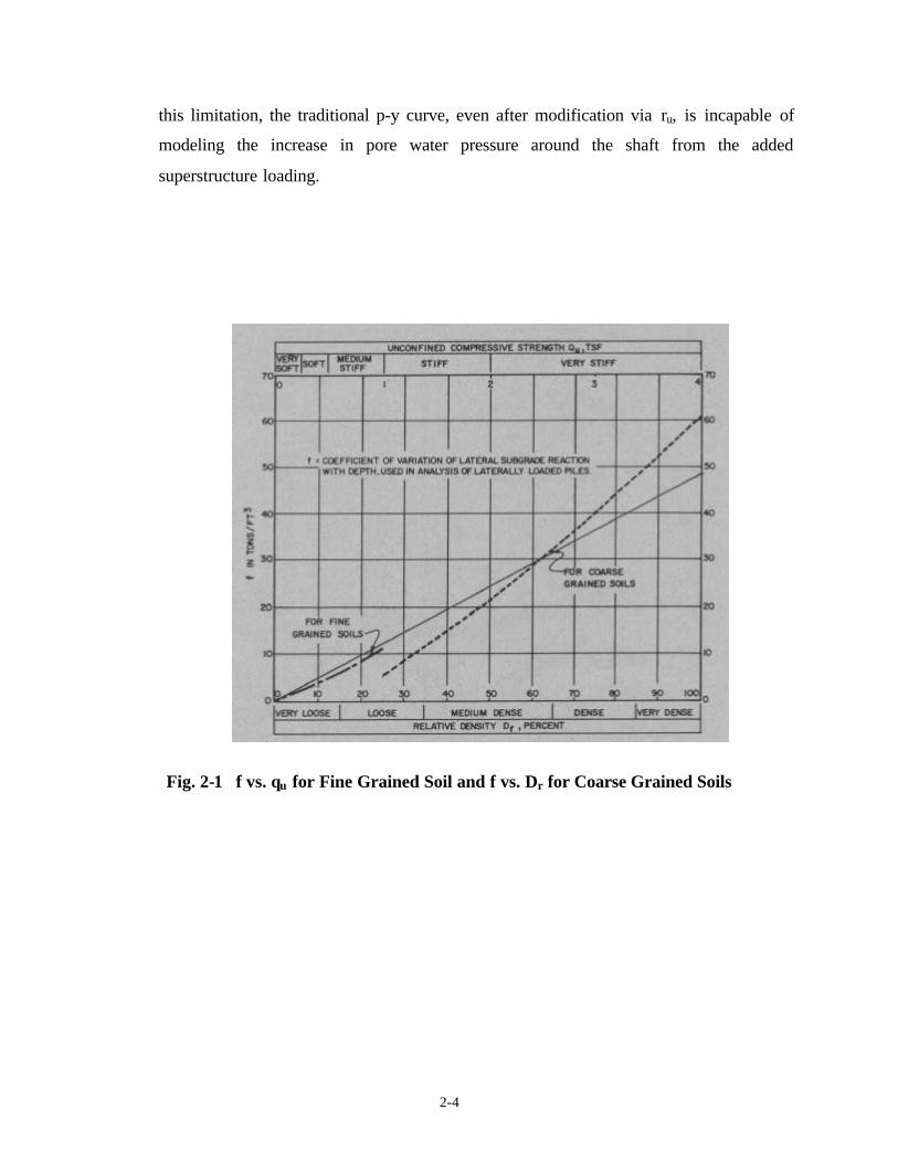
and decreases with increasing lateral load. The chart (Fig. 2-1) attributable to Terzaghi (DM 7.2,
NAVFAC 1982) and modified by Norris (1986) provides average values of f as a function of soil
properties only (independent of pile shape, EI, head fixity, etc).
The shaft behaves as an “intermediate” shaft when [4 > (L/T) > 2]. When an intermediate shaft
is analyzed as a long shaft it results in overestimated lateral response. It should be noted that the
classification of the shaft type in the present study (i.e. evaluation of its relative stiffness, T) is
based on the initial bending stiffness of the shaft and an average of the coefficient of subgrade
reaction (f) including the free-field liquefaction effect.

2-2
The shaft classification for the same shaft my change according to the level loading and the
conditions (e.g. liquefied or non-liquefied) of the surrounding soils. In addition, shaft stiffness
also varies with level of loading and the induced bending moment along the shaft. Therefore, the
criterion mentioned above is not accurate and does not reflect the actual type of shaft with the
progressive state of loading. For example, a shaft could behave as a long shaft under static
loading and then respond as an intermediate shaft under developing liquefaction. Such response
is due to the changing conditions of the surrounding soil. The analysis carried out in this study
changes according to the type of shafts.
2.2 FOUNDATION STIFFNESS MATRIX
The structural engineer targets the shaft-head stiffness (at the base of the column) in 6 degrees of
freedom as seen in Figs. 2-2 through and 2-4. In reality, the bending stiffness (EI) of the cross
section varies with moment. In order to deal with an equivalent linear elastic behavior, a
constant reduced bending stiffness (EIr) for the shaft cross section can be used to account for the
effect of the cracked concrete section under applied loads. However, it is very difficult to
identify the appropriate reduction ratio for the shaft stiffness at a particular level of loading. The
technique presented in this report allows the assessment of the displacement and rotational
stiffness based on the varying bending stiffness of the shaft loaded. Such nonlinear modeling of
shaft material reflects a realistic representation for the shaft behavior according to the level of
loading, and the nonlinear response of shaft material and the surrounding soil The structural
engineer can also replace the nonlinear shaft-head stiffnesses shown in Figs. 2-3 and 2-4 by
using the shaft foundation and the p-y curve resulting from the presented technique along with
the superstructure (complete solution) to model the superstructure-soil-shaft behavior as shown
in Fig 2-6.
2.3 LARGE DIAMETER SHAFT
The computer programs LPILE/COM624P have been developed using lateral load tests
performed on long slender piles. The Vertical Shear Resistance (Vv) acting along the pile or
shaft perimeter has no significant influence on the lateral response of shafts and piles of
diameters less than 3 feet. However, Vv contributes significantly to the capacity of large
diameter shafts. The shaft analysis presented in this report accounts for the Horizontal and

2-3
Vertical Shear Resistance (Vh and Vv) acting along the sides of large diameter shafts in addition
to base resistance (Fig. 2-7). The t-z curve for soil (sand, clay, c-ϕ soil and rock) is evaluated
and employed in the analysis to account for the vertical shear resistance.
It should be noted herein that there are basic differences between the traditional p-y curves used
with LPILE/COM624P and the Strain Wedge (SW) model technique employed in the current
Shaft analysis.
• The traditional p-y relationships used in LPILE/COM624P do not account for the vertical
side shear (Vv) acting along the sides of large diameter shafts because these relationships
were developed for piles with small diameters where side shear is not significant.
• The traditional p-y relationships used in LPILE/COM624P were developed for long piles
and not for intermediate/short shafts or piles. The p-y relationships for long piles are
stiffer than those of short piles/shafts and their direct use in the analysis of short shafts is
not realistic.
• The traditional p-y relationships for sand used in LPILE/COM624P are multiplied,
without any explanation, by an empirical correction factor of 1.55 (Morrison and Reese,
1986)
• The bending stiffness of the pile/shaft has a marked effect on the nature of the resulting
p-y curve relationship. The traditional p-y relationships used in LPILE/COM624P do not
consider this effect. That is, the traditional p-y relationships used in LPILE/COM624P
were developed for piles with diameters less than 3 feet that have much lower values of
bending stiffness (EI) than the large diameter shafts.
• The traditional p-y curves for sand, developed about 30 years ago, is based on a static
load test of a 2-ft diameter long steel pipe pile. They do not consider soil liquefaction.
• The traditional p-y curves have no direct link with the stress-strain relationship of the
soil. Therefore, it is not feasible to incorporate the actual stress-strain behavior of
liquefied soil in the traditional p-y curve formula.
• The traditional p-y curve cannot account for the varying pore water pressure in liquefied
soil. It can only consider the pore water pressure ratio (ru) in the free field (away from
the shaft) by reducing the effective unit weight of soil by a ratio equal to ru. Because of
2-4
this limitation, the traditional p-y curve, even after modification via ru, is incapable of
modeling the increase in pore water pressure around the shaft from the added
superstructure loading.
Fig. 2-1 f vs. qu for Fine Grained Soil and f vs. Dr for Coarse Grained Soils

2-5
Fig. 2-2 Bridge Shaft Foundation and Its Global Axes
Single Shaft

2-6
Fig
. 2-3
F
ound
atio
n St
iffn
esse
s fo
r a
Sing
le S
haft
P2
K22
K11
K66
P1
M3
Y Y
XX
P2
K22
K33
K44
P3
M1
Y Y
ZZ
A)
Loa
ding
in th
e X
-X D
irec
tion
(Axi
s 1)
B)
Loa
ding
in th
e Z
-Z D
irec
tion
(Axi
s 3)
Sin
gle
Sha
ft

2-7
Fig. 2-4 Foundation Springs at the Base of a Bridge Column
in The X-X Direction.
Y
X X
Z
Z
Y
Foundation Springs in
the Longitudinal Direction
K11
K22K66
Column Nodes

2-8
Fig. 2-6 Superstructure-Shaft-Soil Modeling as a Beam on Elastic Foundation (BEF)
y
p
p
p
p
y
y
y
p
y
(Es)1
(Es)2
(Es)3
(Es)4
(Es)5
Ph
Pa

2-9
Fig. 2-7 Configuration of a Large Diameter Shaft
y
p
Soil-Shaft Horizontal Resistance
Po
M o
Vt
Ft
Vv
Vv
FP
FP
FP
Vh
Vh
Vh
M t
Z
T
Soil-Shaft Side Shear Resistance
Po
M o
P V PV
FP
FP
FP
Fv
Fv
Fv
Ft
M t
Vt
MR
MR
MR
3-1
CHAPTER 3
VERTICAL SIDE SHAER AND PILE POINT TIP RESISTANCE OF
A PILE / SHAFT IN CLAY
3.1 INTRODUCTION
The primary focus of this chapter is the evaluation of the vertical side shear induced by
the vertical displacement accompanying the deflection of a laterally loaded shaft. The
prediction of the vertical side shear of a laterally loaded shaft is not feasible unless a
relationship between the vertical shaft displacement and the associated shear resistance is
first established. The most common means to date is the t-z curve method proposed by
Seed and Reese (1957). The associated curves were developed using experimental data
from the vane shear test to represent the relationship between the induced shear stress
(due to load transfer) and vertical movement (z) along the side of the pile shaft (Fig. 3-1).
Other procedures are available to generate the t-z curve along the pile shaft (Coyle and
Reese 1966; Grosch and Reese 1980; Holmquist and Matlock 1976 etc.). Most of these
procedures are empirical and based on field and experimental data. Others are based on
theoretical concepts such as the methods presented by Randolph and Worth (1978), Kraft
et al. (1981) in addition to the numerical techniques adopted by Poulos and Davis (1968),
Butterfield and Banerjee (1971), and the finite element method.
It should be noted that any developed t-z relationship is a function of the pile/shaft and
soil properties (such as shaft diameter, cross section shape and material, axial stiffness,
method of installation and clay shear stress-strain-strength). This requires the
incorporation of as many soil and pile properties as useful and practical in the suggested
analysis.
Coyle and Reese (1966) presented an analytical method to assess the load transfer
relationship for piles in clay. The method is addressed in this chapter and requires the
use of a t-z curve such as those curves suggested by Seed and Reese (1957), and Coyle
and Reese (1966) shown in Figs. 3-1 and 3-2. However, the t-z curve presented by Seed

3-2
and Reese (1957) is based on the vane shear test, and the t-z curve developed by Coyle
and Reese (1966) is based on data obtained from a number of pile load tests from the
field (Fig. 3-2).
The current chapter presents a procedure for evaluating the change in the axial load with
depth for piles in clay called “friction” piles since most of the axial load is carried by the
shaft (as opposed to the pile point). The load transfer mechanism presented by Coyle and
Reese (1966) is used in the proposed analysis in association with the t-z curve developed
herein. In fact, the axially loaded pile analysis is just a means to develop the nonlinear t-
z curves for clay that will be used later to assess the vertical side shear resistance of a
laterally loaded large diameter shaft undergoing vertical movement at its edges as it
rotates from vertical.
3.2 LOAD TRANSFER AND PILE SETTLEMENT
In order to construct the load transfer and pile-head movement in clay under vertical load,
the t-z curve for that particular soil should be assessed. The load transferred from shaft
skin to the surrounding clay soil is a function of the diameter and the surface roughness
of the shaft, clay properties (cohesion, type of consolidation and level of disturbance) in
addition to the shaft base resistance. The development of a representative procedure
allows the assessment of the t-z curve in soil (sand and/or clay) that leads to the
prediction of a nonlinear vertical load-settlement response at the shaft head. Such a
relationship provides the mobilized shaft-head settlement under axial load and the ration
of load displacement or vertical pile head stiffness.
The procedure developed by Coyle and Reese (1966) to assess the load-settlement curve
is employed in this section. However, such a procedure requires knowledge of the t-z
curves (theoretical or experimental) that represent the load transfer to the surrounding soil
at a particular depth for the pile movement (z).
The following steps present the procedure that is employed to assess the load transfer and
pile movement in clay soil:

3-3
1. Based on Skempton assumptions (1951), assume a small shaft base resistance, qP
(small percentage of qnet = 9 C).
qP = 9 Cm = 9 C SL = SL qnet (3-1)
QP = qP Abase = SL qnet Abase (3-2)
C is equal to the clay undrained shear strength, Su. Abase is the area of the pile tip
(shaft base).
2. Using the SL evaluated above and the stress-strain relationship presented in
Chapter 5 [Norris (1986) and Ashour et al. (1998)], compute the induced axial
(deviatoric) soil strain, εP and the shaft base displacement, zP
zP = εP B (3-3)
where B the diameter of the shaft base. See Section 3-3 for more details.
3. Divide the pile length into segments equal in length (hs). Take the load QB at the
base of the bottom segment as (QP) and movement at its base (zB) equal to (zP).
Estimate a midpoint movement for the bottom segment (segment 4 as seen in Fig.
3-3). For the first trial, the midpoint movement can be assumed equal to the shaft
base movement.
4. Calculate the elastic axial deformation of the bottom half of this segment,
base
sB
AE
hQ 2/z elastic = (3-4)
The total movement of the midpoint in the bottom segment (segment 4) is equal to
elasticT zzz += (3-5)
5. Based on the soil properties of the surrounding soil (Su and ε50), use a Ramberg-
Osgood formula (Eqn. 3-6) to characterize the backbone response (Richart 1975).

3-4
+==
−1
1
R
ultultrrz
z
ττ
βττ
γγ
(3-6)
z = total midpoint movement of a pile/shaft segment
γ = average shear strain in soil adjacent to the shaft segment
τ = average shear stress in soil adjacent to the shaft segment
γr is the reference strain, as shown in Fig. 3-4, and equals to Gi / τult
zr = shaft segment movement associated to γr
ε50 = axial strain at SL = 0.5 (i.e. σd = Su). ε50 can be obtained from the chart
provided in Chapter 5 using the value of Su.
β and R-1 are the fitting parameters of the a Ramberg-Osgood model given in
Eqn. 3-7. These parameters are evaluated in section 3.2.1.
6. Using Eqn. 3-6 which is rewritten in the form of Eqn. 3-7, the average shear stress
level (SLt = τ / τult) in clay around the shaft segment can be obtained iteratively based
on movement z evaluated in Eqn. 3-5.
( )[ ]11 −+== Rtt
rr
SLSLz
z βγγ
(Solved for SLt) (3-7)
7. Shear stress at clay-shaft contact surface is then calculated, i.e.
τ = SLt τult or τ = SLt α C (3-8)
where α is the ratio of CA/C that expresses the variation in the cohesion of the
disturbed clay (CA) due to pile installation and freeze, as seen in Fig. 3-5 (DM7.2
, 1986). It should be noted that the drop in soil cohesion is accompanied by a
drop in the initial shear modulus (Gi) of the clay

3-5
8. The axial load carried by the shaft segment in skin friction / adhesion (Qs) is
expressed as
Qs = π B Hs τ (3-9)
9. Calculate the total axial load (Qi) carried at the top of the bottom segment (i = 4).
Qi = Qs + QB (3-10)
10. Determine the elastic deformation in the bottom half of the bottom segment
assuming a linear variation of the load distribution along the segment.
Qmid = (Qi + QB) / 2 (3-11)
EA8
H )Q 3 (Q/
2
Q z sBimid
elastic
+=
+
= EAHQ
sB (3-12)
11. Compute the new midpoint movement of the bottom segment.
z = zP + zelastic (3-13)
12. Compare the z value calculated from step 11 with the previously evaluated
estimated movement of the midpoint from step 4 and check the tolerance.
13. Repeat steps 4 through 12 using the new values of z and Qmid until convergence is
achieved
14. Calculate the movement at the top of the segment i= 4 as
EA
HQQzz sBi
Bi 2
++=
15. The load at the base (QB) of segment i = 3 is taken equal to Q4 (i.e. Qi+1) while zB
of segment 3 is taken equal to z4 and steps 4-13 are repeated until convergence for
segment 3 is obtained. This procedure is repeated for successive segments going
up until reaching the top of the pile where pile head load Q is Q1 and pile top

3-6
movement δ is z1. Based on presented procedure, a set of pile-head load-
settlement coordinate values (Q - δ) can be obtained on coordinate pair for each
assumed value of QT . As a result the load transferred to the soil along the length
of the pile can be calculated for any load increment.
16. Knowing the shear stress (τ) and the associated displacement at each depth (i.e.
the midpoint of the pile segment), points on the t-z curve can be assessed at each
new load.
3.3 DEVELOPED t-z CURVE RELATIONSHIP
For a given displacement (z), the mobilized shear stress (τ) at the shaft-soil interface can
be expressed as a function of the ultimate shear strength (τult) via the shear stress level
(SLt).
SLt = τ / τult (3-14)
The shear displacement of the soil around the pile decreases with increasing distance
from the pile wall (Fig. 3-6). Based on a model study (Robinsky and Morrison 1964) of
the soil displacement pattern adjacent to a vertically loaded pile, it has been estimated
(Norris, 1986) that the average shear strain, γ, within a zone of B/2 wide adjacent to the
pile accounts for 75% of the shear displacement, z, as shown in Fig. 3-7. A linear shear
strain, γ, in the influenced zone (B/2) can be expressed as
B
z
B
z 5.1
2/
75.0 ==γ (3-15)
Therefore,
5.1
Bz
γ= (3-16)
As seen in Fig. 3-7 and because z is directly related to γ based on shaft diameter (Eqn.3-
16), note that

3-7
ffz
z
γγ 5050 = (3-17)
where z50 and γ50 are the shaft displacement and the associated shear strain in the soil at
SLt = 0.5 (i.e. τ = 0.5 τult). zf and γf are the shaft displacement and the associated shear
strain at failure where SLt = 1.0 (i.e. τ = τult). Therefore, the variation in the shear strain
(γ) occurs in concert with the variation in shaft displacement z (Fig. 3-4). It should be
noted that soil shear modulus (G) exhibits its lowest value next to the pile skin and
increases with distance away from the pile to reach it is maximum value (Gi) at γ and z ≅
0 (Fig. 3-6). Contrary to the shear modulus, the vertical displacement (z) and the shear
strain (γ) reach their maximum value in the soil adjacent to the pile face and decrease
with increasing radial distance from the pile.
3.3.1 Ramberg-Osgood Model for Clay
With the above mentioned transformation of the t-z curves to τ-γ curves, a Ramberg-
Osgood model represented by Eqn. 3-6 can be used to characterize the t-z curve.
+==
−1
1
R
ultultrrz
z
ττ
βττ
γγ
(3-18)
At τ/τult = 1 then
1−=r
f
γ
γβ (3-19)
At τ/τult = 0.5 and γ = γ50, then
)5.0(log
1
12
log
)5.0(log
12
log
1
5050
−
−
=
−
=− r
f
rr
Rγγγγ
βγγ
(3-20)

3-8
The initial shear modulus (Gi) and the shear modulus (G50) at SL = 0.5 can be determined
via their direct relationship with the normal stress-strain relationship and Poisson’s ratio
(ν)
3)1(2 G i
ii EE=
+=
νν for clay = 0.5 (3-21)
and
50
505050 33)1(2
Gεν
uSEE==
+= (3-22)
As seen in Fig. 3-4,
i
ult
i
ur GG
S τγ == (3-23)
5050
5.0
G
Su=γ (3-24)
The shear strain at failure (γf) is determined in terms of the normal strain at failure (εf),
i.e.
5.1)1(
ff
f
ε
ν
εγ =
+= (3-25)
The normal stress-strain relationship of clay (σd - ε) is assessed based on the procedure
presented in Chapter 5 that utilizes ε50 and Su of clay. The initial Young’s modulus of
clay (Ei) is determined at a very small value of the normal strain (ε) or stress level (SL).
In the same fashion, εf is evaluated at SL = 1 or the normal strength σdf = 2Su.
3.4 PILE TIP (SHAFT BASE) RESISTANCE IN CLAY
In regard to the pile tip resistance (QT – zT) response, the concept of Skempton’s
characterization (1951) is used as follows,

3-9
basebasenetT ACAqQ 9==
where clay cohesion, C, represents the undrained shear strength, Su. The stress level (SL
= σd / σdf) in clay is proportional to the pressure level (PL = q/qnet). Different from the
strain-deflection relationship established by Skempton (1951) for strip footing (y50 = 2.5
ε50 B), the vertical soil strain (ε1) beneath the base of the shaft is expressed as
EEE321
1
σν
σν
σε
∆+
∆+
∆=
for σ2 = σ3 and ν = 0.5, then
EE331
1 )21(σ
νσσ
ε∆
−+∆−∆
=
EEdσσσ
ε∆
=∆−∆
= 311
Therefore, for a constant Young’s modulus (E) with depth, the strain or ε1 profile has the
same shape as the elastic (∆σ1 - ∆σ3) variation or Schmertmann’s Iz factor (Schmertmann
1970, Schmertmann et al. 1979 and Norris 1986). Taking ε1 at depth B/2 below the shaft
base (the peak of the Iz curve), the shaft base displacement (zT) is a function of the area of
the triangular variation (Fig. 3-9), or
BzT ε= (3-26)
Dealing with different values for the pile tip resistance, the associated deviatoric stress (ε)
and base movement (a function of strain, ε) can be determined (given the stress-strain, σd
- ε relationship of the clay immediately below pile tip) in order to construct the pile point
load-point displacement curve.
3.5 PROCEDURE VALIDATION
3.5.1 Comparison with the Seed-Reese t-z Curve in Soft Clay (California Test)
The test reported by Seed and Reese (1957) was conducted in the San Francisco Bay area
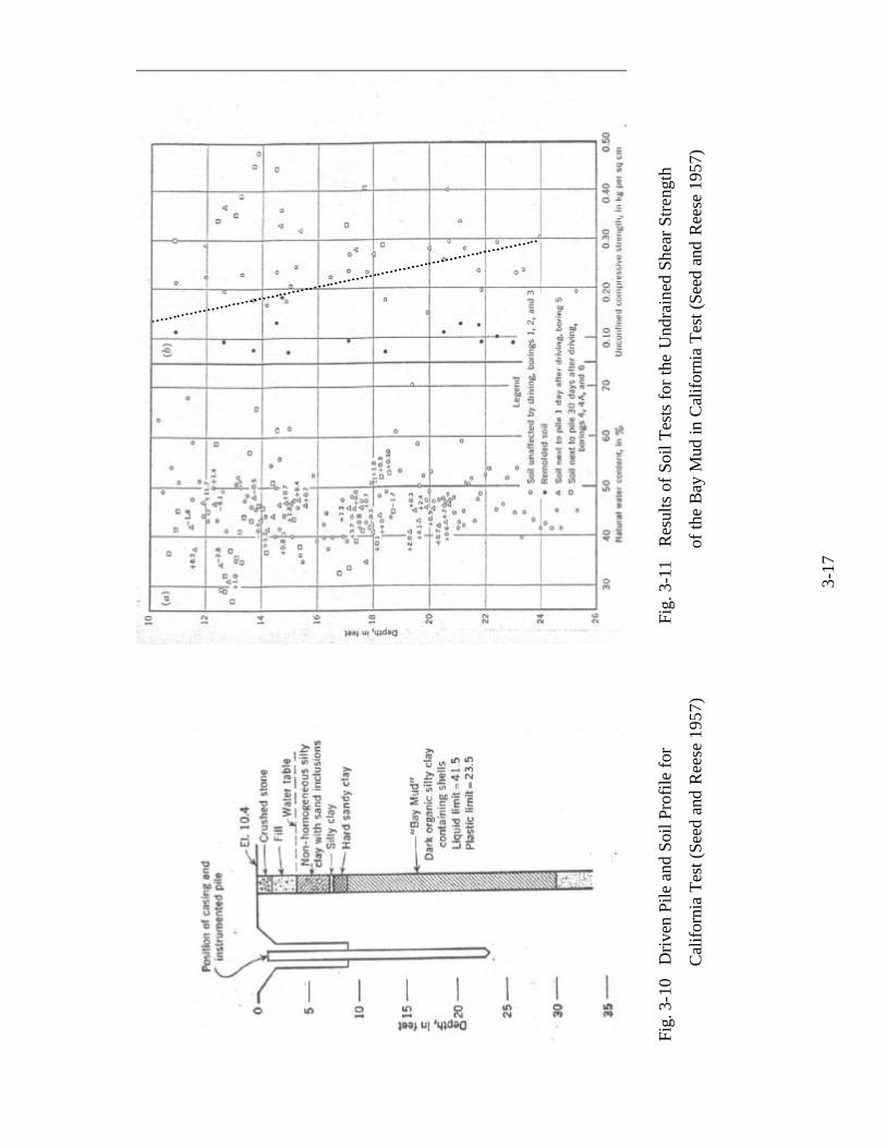
of California. As shown in Fig. 3-10, the soil conditions at that site consisted of 4 ft of

3-10
fill, 5 ft of sandy clay, and around 21 ft of organic soft clay “bay mud”. The water table
was approximately 4 ft below ground.
Several 6-in.-diameter pipe piles (20 to 22 ft long) were driven into the above soil profile.
The pipe pile had a coned tip and maximum load of 6000 lb. The top 9 ft of the
nonhemogeneous soil was cased leaving an embedment in clay of 13 ft.
A number of disturbed and undisturbed unconfined compression tests were conducted to
determine the unconfined compressive strength of clay (Fig. 3-11). Seven loading tests
were performed on the same pile at different periods of time that ranged from 3 hours to
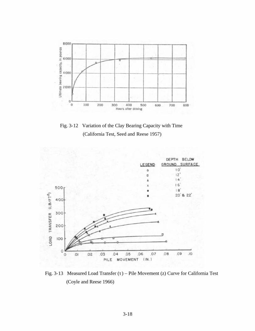
33 days. As shown in Fig. 3-12, the ultimate bearing capacity of the clay reached a stable
and constant value (6200 lb) by the time of the seventh test. As a result, Coyle and Reese
(1966) considered the results of the seventh load test as representative for stable load
transfer-pile movement response.
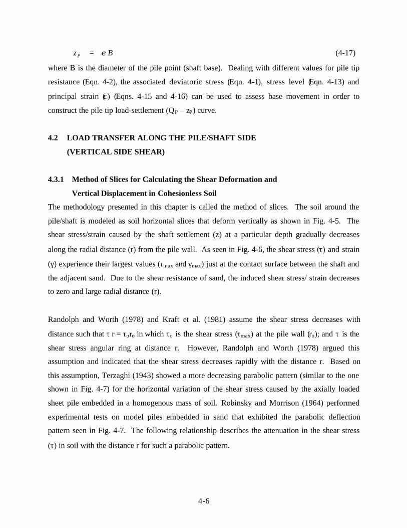
Coyle and Reese (1966) used the data obtained from the current field test conducted by
Seed and Reese (1957) to compute the values of the load transfer response and pile
movement at different depths as seen in Fig. 3-13. Figure 3-14 exhibits an equivalent set
of the t-z curves at the same depths that are constructed by using the procedure presented
herein and based on the undrained compressive strength of clay that is described by the
dashed line shown in Fig. 3-11. The good agreement between the experimental and
predicted t-z curves can be seen in the comparison presented in Fig. 3-15. Such
agreement speaks to capability of the technique presented. The predicted t-z curve at the
deepest two points (20 and 22 feet below ground) and seen in Fig. 3-15 can be improved
by a slight increase in the undrained compressive strength utilized.
The good agreement between the predicted and experimental t-z curves resulted in an
excellent assessment for load distribution (due to shear resistance) along the pile. Fig. 3-
16 shows the assessed load distribution and tip resistance that are based on the procedure
presented and induced in 1000-lb axial load increments up to an axial load of 6000 lb. A
3-11
comparison between the measured and predicted load distributions along the pile is
shown in Fig. 3-17.
The measured pile head load-settlement curves under seven cases of axial loads are
shown in Fig. 3-18. The loading tests were performed at different periods of time after
driving the pile. As mentioned earlier, the seventh test (after 33 days of driving the pile)
is considered for the validation of the procedure presented. Reasonable agreement can be
observed between the predicted and measured pile head load-settlement curve (Fig. 3-
18).
It should be noted that Seed and Reese (1957) established a procedure that allows the
assessment of the pile load-settlement curve and the distribution of the pile skin
resistance based on the data collected from vane shear test shown in Fig. 3-1. In addition,
some assumptions should be made for the point load movement in order to get good
agreement with the actual pile response. Seed and Reese (1957) presented explanation for
the lack of agreement between their calculated and measured data. The undrained
compressive strength collected using the vane shear test was the major source of that
disagreement.
3.6 SUMMARY
The procedure to evaluate the t-z and load-settlement curves for a pile in clay presented
here is based on elastic theory and Ramberg-Osgood characterization of the stress-strain
behavior of soil. This procedure allows the assessment of the mobilized resistance of the
pile using the developed t-z curve and the pile point load-displacement relationship. The
results obtained in comparison with the field data show the capability and the flexible
nature of the suggested technique. Based on the comparison study presented in this
chapter, the good agreement between the measured and predicted load transfer along the
pile, pile movement, pile-head settlement and pile tip resistance shows the consistency of
the technique’s assumptions. The findings in this chapter will be employed in Chapter 5
to evaluate the vertical side shear resistance induced by the lateral deflection of a large
diameter shaft and its contribution to the lateral resistance of the shaft.

3-12
Fig. 3-1 Shear Resistance vs. Movement Determined by the Vane Shear Test
(Seed and Reese 1957)
Fig. 3-2 Ratio of Load Transfer to Soil Shear Strength Vs. Pile Movement
for a Number of Field Tests (Coyle and Reese 1966)

3-13
Fig. 3-3 Modeling Axially Loaded Pile Divided into Segments
V v1 V v1
(z mid)1
Q = Q1
V v2 V v2
Q2
V v3 V v3
Q3
V v4 V v4
Q4
QP
z = z1
zP
L
Q1
Q3
Q4
QP
z P
h
h
h
h
Segment 1
Segment 2
Segment 3
Segment 4
Segment 1
Segment 2
Segment 3
Segment 4
=
(EA/h )1
(EA/h)2
(EA/h)3
z = z 2
(z mid)2
(z mid)3
(zmid)4
z = z3
z = z4
(zmid)4
z = z4
z = z 3
Q = Q1
z = z 1
(zmid)1
z = z 2
(zmid)2
(zmid)3

3-14
Fig. 3-4 Basic (Normal or Shear) Stress-Strain Curve
Fig. 3-5 Changes in Clay Cohesion Adjacent to the Pile Due to Pile Installation
(DM7.2 1986)
ε or γεr or γr
σult or τultσ
or τ
Ei or Gi
ε50 or γ50
σ50 or τ50

3-15
Fig. 3-6 Soil Layer Deformations Around Axially Loaded Pile
Fig. 3-7 Idealized Relationship Between Shear Strain in Soil (γ)
and Pile Displacement (Z) (Norris, 1986)
B
B/2
0.75 zγ
z
Qo
QT
Sheared soil layers

3-16
Fig. 3-8 Soil Shear Resistance Vs. Shear Strain (γ) or Pile Movement (z)
Fig. 3-9 Schmertmann Strain Distribution Below Foundation Base
(after Norris, 1986)
z or γ
τultτ
z50 or γ50
τ50
zf or γf
ε = σd / E
B/2
B
2B
D
3-17
Fig.
3-1
0 D
rive
n P
ile
and
Soi
l Pro
file
for
F
ig. 3
-11
Res
ults
of
Soi
l Tes
ts f
or th
e U
ndra
ined
She
ar S
tren
gth
C
alif
orni
a T
est (
See
d an
d R
eese
195
7)
of
the
Bay
Mud
in C
alif
orni
a T
est (
Seed
and
Ree
se 1
957)
3-18
Fig. 3-12 Variation of the Clay Bearing Capacity with Time
(California Test, Seed and Reese 1957)
Fig. 3-13 Measured Load Transfer (τ) – Pile Movement (z) Curve for California Test
(Coyle and Reese 1966)

3-19
Fig. 3-14 Predicted Load Transfer (τ) – Pile Movement (z) Curve for
California Test Using the Suggested Procedure
Fig. 3-15 Comparison Between Measured and Predicted Load Transfer (τ) – Pile
Movement (z) Curve for the California Test
0 0.02 0.04 0.06 0.08 0.1Pile Movement, z, in
0
100
200
300
400
500Lo
ad T
rans
fer,
t, lb
/ft2
Measured Predicted

3-20
Fig.
3-1
6 P
redi
cted
Loa
d D
istr
ibut
ion
alon
g F
ig. 3
-17
Com
pari
son
of M
easu
red
and
Pre
dict
ed L
oad
Dis
trib
utio
n
the
Pile
in
Cal
ifor
nia
Tes
t
alo
ng th
e P
ile in
Cal
ifor
nia
Tes
t (S
eed
and
Ree
se 1
957)
020
0040
0060
0080
00
Pile
-Hea
d A
xial
Loa
d, lb
24222018161412108
Depth, ft

3-21
Fig. 3-18 Pile-Head Load-Settlement Curves for Seven Loading Tests at Different Time
Periods for the California Test in Comparison with the Predicted Results
Predicted

4-1
CHAPTER 4
VERTICAL SIDE SHAER AND POINT RESISTANCE OF
PILE/SHAFT IN SAND
4.1 INTRODUCTION
The friction pile in cohesionless soil gains its support from the pile tip resistance and the transfer
of load via the pile wall along its length. It has been suggested that the load transferred by skin
friction pile can be neglected which is not always the case. The load transferred via the pile wall
depends on the diameter and length of the pile, the surface roughness, and soil properties. It
should also be mentioned that both pile point and skin resistances are interdependent.
The assessment of the mobilized load transfer of a pile in sand depends on the success in
developing a representative t-z relationship. This can be achieved via empirical relationships
(Kraft et al. 1981) or numerical methods (Randolph and Worth, 1978). The semi-empirical
procedure presented in this chapter employs the stress-strain relationship of sand and findings
from experimental tests. The t-z curve obtained based on the current study will be used in
Chapter 5 to account for the vertical side shear resistance that develops with the laterally loaded
large diameter shafts.
The method of slices presented in this chapter reflects the analytical portion of this technique that
allows the assessment of the attenuating shear stress/strain and vertical displacement within the
vicinity of the driven pile. As a result, the load transfer and the t-z curve can be assessed using a
combination between the tip and side resistances of the pile.
PILE POINT (SHAFT BASE) RESISTANCE AND SETTLEMENT
(QP – zP) IN SAND
It is evident that the associated pile tip resistance manipulates the side resistance of the pile shaft.
As presented in the analysis procedure, the pile tip resistance should be assumed at the first step.
As a result, the shear resistance and displacement of the upper segments of the pile can be

4-2
computed based on the assumed pile tip movement. This indicates the need for a practical
technique that allows the assessment of the pile tip load-displacement relationship under a
mobilized or developing state. Most of the available techniques provide the ultimate pile tip
resistance that is independent of the specified settlement. In other words, the pile tip settlement
at the ultimate tip resistance is a function of the pile diameter (e.g. 5 to 10% of pile tip diameter).
Thereafter, a hyperbolic curve is used to describe the load-settlement curve based on the
estimated ultimate resistance and settlement of the pile tip.
Elfass (2001) developed an approach that allows the assessment of the mobilized pile tip
resistance in sand and the accompanying settlement over the whole range of soil strain up to and
beyond soil failure. In association with the pile side shear resistance technique presented in
Section 4-2, the approach established by Elfass (2001) will be employed in the current study to
compute the pile tip load-settlement in sand.
The failure mechanism developed by Elfass (2001) assumes four failure zones represented by
four Mohr circles as shown in Fig. 4.1. This mechanism yields the bearing capacity (q) and its
relationship with the deviatoric stress (σd) of the last (fourth Mohr circle) as shown in Fig 4-2. .
qd 6.0=σ (4-1)
The pile tip resistance (QP ) is given as,
based
baseP AAqQ6.0
σ== (4-2)
where Abase is the cross sectional area of the pile tip (shaft base).
As seen in Fig. 4-1, the Mohr Columb strength envelope is nonlinear and requires the evaluation
of the secant angle of the fourth circle (ϕIV) tangent to the curvilinear envelope. The angle of the
secant line tangent to first circle (ϕI) at effective overburden pressure can be obtained from the
field blow data count (SPT test) or a laboratory triaxial test at approximately 1 tsf (100 kPa)
confining pressure. Due to the increase in the confining pressure )( 3σ from one circle to the

4-3
next, the friction angle (ϕ) decreases from ϕI at I)( 3σ to ϕIV at IV)( 3σ based on the following
Bolton (1986) relationship modified by Elfass (2001) (Fig. 4-3)
diffpeak ϕϕϕ += min (4-3)
( )1
3
2/45tan2ln1033 3
2
−
++−== σϕϕ RRdiff DI (4-4)
3σ is in kPa. ϕmin is the lowest friction angle that ϕ may reach at high confining pressure, as
shown in Fig. 4-4 and Dr is inputted as its decimal value.
Knowing the sand relative density (Dr) and the associated friction angle under the original
confining pressure )( 3 voσσ = , the reduction in the friction angle (∆ϕ) due to the increase of the
confining pressure from voσ to IV)( 3σ can be evaluated based on Eqns. 4-3 and 4-4, as
described in the following steps:
1. Based on Eqn. 4-4, calculate (ϕdiff)I at the original confining pressure )( 3 voσσ =
( )1
3
2/45tan2ln103)(
2
−
++−= voI
RIdiff D σϕϕ (4-5)
2. Assume a value for the deviatoric stress (σd) of the fourth circle (Fig. 4-2). As a result,
6.0 q dσ
= (4-6)
qq vodvoIV 4.0)( 3 +=−+= σσσσ (4-7)
3. Assume a reduction (∆ϕ = 3 or 4 degrees) in the sand friction angle at )( 3 voσσ =
due to the increase in the confining pressure from voσ to IV)( 3σ , as seen in Fig. 4-4.
Therefore,
ϕIV = ϕI - ∆ϕ (4-8)

4-4
4. As presented by Elfass (2001) and shown in Fig. 4-4, ϕ changes in a linear pattern with
the logarithmic increase of 3σ . The friction angle ϕIV associated with the confining
pressure IV)( 3σ can be calculated as
vo
IVIIV σ
σϕϕϕ
)(log
3∆−= (4-9)
5. According to the computed friction angle (ϕIV), use Eqn. 4-4 to evaluate (ϕdiff)IV.
( )1)(
3
2/45tan2ln103)( 3
2
−
++−= IV
IVRVIdiff D σ
ϕϕ (4-10)
6. Having the values of (ϕdiff)I and (ϕdiff)IV, a revised value for ∆ϕ can be obtained.
∆ϕ = (ϕdiff)I - (ϕdiff)IV (4-11)
7. Compare the value of ∆ϕ obtained in step 6 with the assumed ∆ϕ in step3. If they are
different, take the new value and repeat the steps 3 through 7 until the value of ϕIV
converges and the difference in ∆ϕ reached is within the targeted tolerance.
8. Using the calculated values of ϕI and ϕIV, the deviatoric stress at failure can be expressed
as
( )( )12/45tan)( 23 −+= IVIVdf ϕσσ (4-12)
9. The current stress level (SL) in soil (Zone 4 below pile tip) is evaluated as
( )( ) dfd
df
d
IV
m SLSL σσσσ
ϕϕ
==−+−+
= ;12/45tan
12/45tan2
2
(4-13)
where
+= −
2/)(
2/sin
3
1
dIV
dm σσ
σϕ (4-14)

4-5
4.2.1 Pile Tip Settlement
As presented in Chapter 3 with clay soil, the pile tip displacement in sand can be determined
based on the drained stress-strain relationship presented in Chapter 5 (Norris 1986 and Ashour et
al. 1998). The soil strain (ε) below the pile tip is evaluated according to the following equations:
Corresponding to a triaxial test at a given confining pressure ( 3σ ) at a deviator stress (σd) and
stress level (SL) as given by Eqns. 4-12 through 4-14.
ελ
ε 50
3.707
SLeSL= (4-15)
The value 3.707 and λ represent the fitting parameters of the power function relationship, and ε50
symbolizes the soil strain at 50 percent stress level. λ is equal to 3.19 for SL less than 0.5 and λ
decreases linearly with SL from 3.19 at 0.5 to 2.14 at SL equal to 0.8.
Equation 4-16 represents the final loading zone which extends from 80 percent to 100 percent
stress level. The following equation is used to assess the strain (ε) in this range:
( ) 0.80 SL q + m
100 + 0.2 = SL ≥
;lnexp
εε
(4-16)
where m=59.0 and q=95.4 ε50 are the required values of the fitting parameters.
The two relationships mentioned above are developed based on unpublished experimental results
(Norris 1977).
For a constant Young’s modulus (E) with depth, the strain or ε1 profile has the same shape as the
elastic (∆σ1 - ∆σ3) variation or Schmertmann’s Iz factor (Schmertmann 1970, Schmertmann et al.
1979 and Norris 1986). Taking ε1 at depth B/2 below the shaft base (the peak of the Iz curve),
the shaft base displacement (zP) is a function of the area of the triangular variation (Fig. 3-9).
4-6
Bz P ε= (4-17)
where B is the diameter of the pile point (shaft base). Dealing with different values for pile tip
resistance (Eqn. 4-2), the associated deviatoric stress (Eqn. 4-1), stress level (Eqn. 4-13) and
principal strain (ε) (Eqns. 4-15 and 4-16) can be used to assess base movement in order to
construct the pile tip load-settlement (QP – zP) curve.
4.2 LOAD TRANSFER ALONG THE PILE/SHAFT SIDE
(VERTICAL SIDE SHEAR)
4.3.1 Method of Slices for Calculating the Shear Deformation and
Vertical Displacement in Cohesionless Soil
The methodology presented in this chapter is called the method of slices. The soil around the
pile/shaft is modeled as soil horizontal slices that deform vertically as shown in Fig. 4-5. The
shear stress/strain caused by the shaft settlement (z) at a particular depth gradually decreases
along the radial distance (r) from the pile wall. As seen in Fig. 4-6, the shear stress (τ) and strain
(γ) experience their largest values (τmax and γmax) just at the contact surface between the shaft and
the adjacent sand. Due to the shear resistance of sand, the induced shear stress/ strain decreases
to zero and large radial distance (r).
Randolph and Worth (1978) and Kraft et al. (1981) assume the shear stress decreases with
distance such that τ r = τoro in which τo is the shear stress (τmax) at the pile wall (ro); and τ is the
shear stress angular ring at distance r. However, Randolph and Worth (1978) argued this
assumption and indicated that the shear stress decreases rapidly with the distance r. Based on
this assumption, Terzaghi (1943) showed a more decreasing parabolic pattern (similar to the one
shown in Fig. 4-7) for the horizontal variation of the shear stress caused by the axially loaded
sheet pile embedded in a homogenous mass of soil. Robinsky and Morrison (1964) performed
experimental tests on model piles embedded in sand that exhibited the parabolic deflection
pattern seen in Fig. 4-7. The following relationship describes the attenuation in the shear stress
(τ) in soil with the distance r for such a parabolic pattern.

4-7
2
2
r
ro
o
=ττ
(4-18)
In order to understand the slice method, the stress-strain conditions of a small soil element at the
contact surface with the pile shaft is analyzed. Figure 4-8 shows the induced shear stress on the
soil-pile contact surface.
The lateral earth pressure coefficient (K) varies, with the radial distance, from 1 at the pile wall
(due to pile installation) to K = Ko = 1 – sin ϕ in the free-field where the z-movement-induced
shear stress (τ) reaches zero. Therefore, the horizontal effective stress at the pile wall after
installation (prior to loading of the pile) just equals the vertical effective overburden, voσ (i.e.
lateral earth pressure coefficient K = 1). It should be noted that τo represents the τmax induced at
the pile wall. Accordingly, a Mohr circle with a center at voσ and a diameter of 2τo (τmax = τo)
develops at r = ro, as shown in Fig. 4-8. With radial distance from the pile, the horizontal normal
stress (σh) and the deviator stress (σd) continue to drop from voσ and 2τmax at ro to )sin1( ϕσ −vo
and )1( ovo K−σ or ϕσ sinvo in the far-field (where τ due to z is 0). The corresponding shear
strain (γ = γmax) causes a major normal strain ε1,
ε1 = (1 + ν) γ (4-19)
In addition, the shear modulus (G) is related to the Young’s modulus (E) at the given effective
confining pressure ( 3σ ) and normal strain (ε1), i.e.
)1(2 ν+= E
G (4-20)
The method of slices described in Fig. 4-10, is based on the shear stress variation concepts
presented above. The proposed method of slices provides the radius of the soil ring (radial
distance, r) over which the induced shear stress diminishes, as shown in Fig. 4-7.

4-8
As shown in Fig. 4-11 for soil ring 1, the horizontal stress (σh) on the soil-pile interface (inner
surface of the first soil slice) is equal to voσ . At the same time, the horizontal stress (σh) on the
outer surface is expressed as
τσσ ∆−= voh (4-21)
The horizontal (radial and tangential) equilibrium is based on the ring action for the whole ring
of soil (2πr) around the pile. The vertical equilibrium is also conducted on a full ring of soil.
The vertical equilibrium of the first soil ring (slice) adjacent to the pile wall is expressed by the
following equations:
∑ = 0yF (4-22)
0coscos 1 =−∆−− WTRR TTBB ϕϕ (4-23)
Therefore,
0coscos 1 =−∆−− WTRR TTBB ϕϕ (4-24)
and
TRRW TTBB ∆−−= ϕϕ coscos1 (4-25)
where ∆T represents the reduction in the vertical shear force along the radial width (∆r) of the
horizontal soil ring.
The following steps explain the implementation of the method of slices:
1. Divide the pile length into a number of segments that are equal in length (Hs). Note that
the effective stress ( voσ ) (i.e. the initial confining stress) increases with depth for each
pile segment.
2. Assume a shear stress developed at the soil-pile interface (r = ro) equal to that at soil
failure or τult. It should be noted that there might be a slip condition (e.g. τlimit = K voσ
tanδ) at the soil pile interface that limits to a value τlimit less than τult.

4-9
3. Determine the developing confining pressure 3σ due to τmax (Fig. 4-11)
ϕσσ sin13 −== vooK (4-26)
where ϕ the friction angle at failure.
4. Increase the radial distance (r) from ro to r1 by a small incremental amount (∆r). As a
result, the vertical shear stress on the face of the slice at r1 will drop to τ1 as expressed in
Eqn. 4-21.
5. The horizontal stress (σh) on the vertical face of the soil slice decreases with the
attenuating shear stress (τ) as shown in Fig. 4-9 until it reaches the value of 3σ given in
Eqn. 4-26. The Mohr circles shown in Fig. 4 describe the decrease in horizontal stress
(σh) and the mobilized friction angle (ϕm) in association to the attenuation in the shear
stress (τ) (and the vertical shear force, T, on a vertical unit length) acting on the vertical
face of the soil ring, i.e.
∆T1 = T0 – T1 = 2π (roτo - r1τ1) (4-27)
)r- (r cos
= R 2o
21
T
1
T πϕ
σ h(4-28)
)r- (r cos
= R 2o
21
B
B πϕ
σvo(4-29)
It should be noted that voσ is the effective stress at the middle of the slice which is used
as an average effective stress for the whole slice (i.e. with More circle). The angles ϕT
and ϕB at the top and bottom of the first soil ring, respectively, are determined as follows,
vo
oB
στ
ϕ 1sin −= (4-30)
111sin τττ
τστ
ϕ −=∆∆−
= −o
voT where (4-31)

4-10
ϕB equals ϕT of the next slice (soil ring 2) where τ1 and τ2 are the vertical shear stresses at
radii r1 and r2, respectively (Fig. 4-12).
6. Based on the induced shear stress (τo) on the inner face of the current soil ring (first ring)
and its Mohr circle, calculate the associated shear strain (γ) that develop over the width
(∆r) of the current soil ring. For each horizontal soil slice i (soil ring with a width ∆r) and
based on the induced shear stress (τ) as seen in Fig. 4-10, the normal strain and stress (ε
and σd), and ν will be evaluated. Thereafter, determine the associating shear strain γi and
vertical displacement zi as follows,
νε
γ+
=1
ii (4-32)
where
iSL4.01.0 +=ν
iii rz ∆= γ (4-33)
7. Repeat steps 1 through 6 for larger values of r (i.e. an additional soil ring) and calculate zi
for each soil slice (ring) until the induced vertical shear stress approaches zero at r = rf.
8. Assess the total vertical displacement at the soil-pile contact (τ = τmax or τo) as follows,
∑=
=
=0τ
ττ o
if zz (4-34)
zf represents the elastic vertical displacement at failure at the soil-pile contact that is
needed to construct the Ramberg-Osgood model in the next sections.
It would be noticed that the soil ring is always in horizontal equilibrium. For example, the
horizontal equilibrium for the first ring of soil can be expressed as
0=∑ xF

4-11
0sinsin 1 =−−+ BBTTo RERE ϕϕ (4-35)
where,
sovoo HrE πσ 2= (4-37)
sv HrE 11 2πσ= (4-38)
vσ varies from voσ at the sand-pile contact surface to )sin1( ϕσ −vo at rf where the induced
shear stress (τ) = 0, as shown in Fig. 4-7.
4.3.2 Ramberg-Osgood Model for Sand
As presented in Chapter 3 with the clay soil, Ramberg-Osgood model represented by Eqn. 4-39
can be used to characterize the t-z curve.
+==
−1
1
R
ultultrrz
z
ττ
βττ
γγ
(4-39)
At τ/τult = 1 then
1−=r
f
γ
γβ (4-40)
At τ/τult = 0.5 and γ = γ50, then
)5.0(log
1
12
log
)5.0(log
12
log
1
5050
−
−
=
−
=− r
f
rr
Rγγγγ
βγγ
(4-41)
The initial shear modulus (Gi) at a very low SL and the shear modulus (G50) at SL = 0.5 can be
determined via their direct relationship with the normal stress-strain relationship and Poisson’s
ration (ν)
4-12
2.2)1(2 G i
ii EE=
+=
νν for sand = 0.1 (4-42)
and
50
505050
3
2/
3)1(2 G
ε
σ
νdfEE
==+
= (4-43)
Therefore,
i
df
i
ultr
GG
2/στγ == (4-44)
The Poisson’s ratio (ν) for sand varies 0.1 to 0.5 with the increasing values of SL as follows,
SL4.01.0 +=ν (4-45)
The shear strain at failure (γf) is determined in terms of the normal strain at failure (εf).
5.1)1(
ff
f
ε
ν
εγ =
+= (4-46)
The normal stress-strain relationship of sand (σd - ε) is assessed based on the procedure
presented in Chapter 5. The initial Young’s modulus of clay (Ei) is determined at a very small
value of the normal strain (ε) or stress level (SL). In the same fashion, εf is evaluated at SL = 1
or the normal strength σdf. By knowing the values of γr, γ50 and γf, the constants β and R of the
Ramberg-Osgood model shown in Eqn. 4-39 can be evaluated.
The Ramberg-Osgood model given in Eqn. 4-39 allows the assessment of the elastic vertical
displacement that occurs at the soil-pile contact surface based on zf obtained in Section 4-3-1.
Equation 4-39 can be rewritten as follows,
+=
−1
1
R
ultultrz
z
ττ
βττ
(4-47)
where,

4-13
f
rfr
f
r
f
r zzeiz
z
γγ
γγ
== .. (4-48)
4.3.3 Procedure Steps to Assess Load Transfer and Pile Settlement
in Sand (t-z Curve)
The assessment of the load transfer and associated settlement of a pile embedded in sand requires
the employment of t-z curve for that particular soil. The load transferred from pile shaft to the
surrounding sand is a function of the diameter and the surface roughness of the pile skin and
sand properties (effective unit weight, friction angle, relative density and confining pressure) in
addition to the pile tip resistance. The development of a representative procedure allows the
assessment of the t-z curve in soil (sand and/or clay) that leads to the prediction of a nonlinear
load-settlement curve at the pile/shaft head. Such a relationship provides the mobilized pile-head
settlement under axial load and vertical shear resistance.
A new procedure is developed in this chapter to assess pile/shaft skin resistance in sand in a
mobilized fashion. The proposed procedure provides the deformation in sand around the pile in
the radial zone affected by the pile movement (Fig. 4-1). At the same time, the horizontal
degradation (attenuation) of the shear stress away from the pile is evaluated by the suggested
analysis. As a result, the varying shear stress/strain, shear modulus and deformation in the radial
distance away from the pile can be predicted based on reasonable assumptions.
The presented t-z curve is developed according to the induced displacement along the pile. The
following steps present the procedure that is employed to assess the load transfer and pile
movement in sand soil:
1. Based on the approach presented in Section 4-2 for the pile tip resistance, assume a small
pile tip resistance, QP as given in Eqns (4-1 and 4-2)

4-14
2. Using the SL evaluated above and the stress-strain relationship presented in Eqns. 4-13
through 4-16, compute the induced axial (deviatoric) soil strain, εP and the shaft base
displacement, zP = εP B. B is the diameter of the shaft base.
3. Divide the pile length into segments equal in length (hs). Take the load QB at the base of
the bottom segment as (QP) and movement at its base (zB) equal to (zP). Estimate a
midpoint movement for the bottom segment (segment 4 as seen in Fig. 4-13). For the
first trial, the midpoint movement can be assumed equal to the shaft base movement.
4. Calculate the elastic axial deformation of the bottom half of this segment,
base
sB
AE
hQ 2/z elastic = (4-49)
The total movement of the midpoint in the bottom segment (segment 4) is equal to
elasticT zzz += (4-50)
5. Based on the soil properties of the surrounding sand, use a Ramberg-Osgood formula to
characterize the backbone response (Richart 1975).
+==
−1
1
R
ultultrrz
z
ττ
βττ
γγ
(4-51)
z = total midpoint movement of a pile/shaft segment
γ = average shear strain in soil adjacent to the shaft segment
τ = average shear stress in soil adjacent to the shaft segment
γr is the reference strain, as shown in Fig. 3-4, and given by Eqn. 4-44
zr = shaft segment movement associated to γr
ε50 = axial strain at SL = 0.5. ε50 can be obtained from the chart provided in Chapter 5.

4-15
β and R-1 are the fitting parameters of the Ramberg-Osgood model given in Eqn. 4-52.
These parameters are evaluated in section 4.2.1.
6. Using Eqn. 4-51 which is rewritten in the form of Eqn. 4-52, the average shear stress
level (SLt) in sand around the shaft segment can be obtained iteratively based on
movement z evaluated in Eqn. 4-50.
( )[ ]11 −+== Rtt
rr
SLSLz
z βγγ
(Solved for SLt) (4-52)
7. Shear stress at soil-shaft contact surface is then calculated, i.e.
τ = SL σdf/2 (4-53)
8. The axial load carried by the shaft segment in skin friction / adhesion (Qs) is
expressed as
Qs = π B hs τ (4-54)
9. Calculate the total axial load (Qi) carried at the top of the bottom segment (i = 4).
Qi = Qs + QB (4-55)
10. Determine the elastic deformation in the bottom half of the bottom segment
assuming a linear variation of the load distribution along the segment.
Qmid = (Qi + QB) / 2 (4-56)
EA8
h )Q 3 (Q/
2
Q z sBimid
elastic
+=
+= EAh
Qs
B (4-57)
11. Compute the new midpoint movement of the bottom segment.

4-16
z = zP + zelastic (4-58)
12. Compare the z value calculated from step 11 with the previously evaluated estimated
movement of the midpoint from step 4 and check the tolerance.
14. Repeat steps 4 through 12 using the new values of z and Qmid until convergence is
achieved
15. Calculate the movement at the top of the segment i= 4 as
EA
hQQzz sBi
Bi2
++=
16. The load at the base (QB) of segment i = 3 is taken equal to Q4 (i.e. Qi+1) while zB of
segment 3 is taken equal to z4 and steps 4-13 are repeated until convergence for segment
3 is obtained. This procedure is repeated for successive segments going up until reaching
the top of the pile where pile head load Q is Q1 and pile top movement δ is z1. Based on
presented procedure, a set of pile-head load-settlement coordinate values (Q - δ) can be
obtained on coordinate pair for each assumed value of QT . As a result the load
transferred to the soil along the length of the pile can be calculated for any load
increment.
17. Knowing the shear stress (τ) and the associated displacement at each depth (i.e. the
midpoint of the pile segment), points on the t-z curve can be assessed at each new load.
4.4 PROCEDURE VALIDATION
As reported by Vesic (1970), an 18-inch diameter steel pipe pile with 0.5-inch-thick walls was
driven and tested in five stages. The bottom section has a 2-in thick flat steel plate at the base of
the pile. Tests with this pile were performed at driving depths of 10, 20, 30, 40 and 50 ft.
Figure, 4-14 shows the results of the standard penetration tests (SPT) at different locations at the
test site. Figure 4-15 the particle size distribution curves of two different types of sands. The

4-17
fine sand curves in this figure refer to the material found mostly at the top 5 ft of the soil profile.
It should be noted that the frictions angles shown in Table 4-1 is a little bit relatively high
compared to the associated (N1)60.
Table 4-1 – Suggested Soil Data for Current Soil Profile
Soil
layer #
Soil type Thickness
(ft)
γ (pcf) (N1)60 φ (deg.) ε50**
1 Sand 10 110 9 30 0.009
2 Sand 10 60 15 32 0.007
3 Sand 10 60 19 35 .006
4 Sand 10 66 24 39 .004
5 Sand 10 66 32 42 0.003
Figure 4-16 exhibits a comparison between the measured and computed data at the depths 20, 40
and 50 ft below ground. Good agreement between the measured and computed axial pile load
can be seen in Fig. 4-16.
4.5 SUMMARY
This Chapter presents a procedure that allows the assessment of the t-z and load-settlement
curves for a pile in sand. The methodology employed is based on the elastic theory, stress-strain
relationship, and the method of slices for the vertical equilibrium. The results obtained
incorporate the pile tip and side resistance in a mobilized fashion. The results obtained in
comparison with the field data show the capability of the suggested technique. The findings of
this chapter will be employed in Chapter 5 to evaluate the vertical side shear resistance induced
by the lateral deflection of a large diameter shaft and its contribution to the lateral resistance of
the shaft.

4-18
Fig. 4-1 Failure Mechanism of Sand Around Pile Tip (Elfass, 2001)
Fig. 4-2 Relationship Between Bearing Capacity (qnet) of Pile Tip in Sand and the Deviatoric
Stress (σd) (after Elfass, 2001)
(σ3)IV (σ1)IV = qult
σvo
ϕI
ϕIV
qnet
σd= 0.6 q
net
Zone IV
Zone Iσ
τ

4-19
Fig. 4-3 Degradation in the Secant Friction Angles of Circles Tangent to a Curvilinear
Envelope of Sand Due to the Increase in the Confining Pressure (Elfass, 2001)
Fig. 4-4 Changes of Friction Angle (ϕ) with the Confining Pressure
ϕ
ϕPeak
ϕdiff
ϕmin
3σ3,Pr σessureConfining
ϕ
∆ϕ
ϕmin
(log)3σ1 10 100

4-20
Fig. 4-5 Soil Deformation in the Vicinity of Axially Loaded Pile.
Qo
QT
Sheared soil layers

4-21
Fig. 4-6 Shear Stress/Strain at Soil-Pile Interface.
Fig. 4-7 Shear and Displacement Attenuation with the Radial Distance from the Pile Wall.
τo
τn
Shaft
rornrn + m
Displacement, z
zmax
Distanceτn + m
zn
Zn + m
Shear Stress, τ
Shaft
σvo
Kσvo
ττ
γ
Shaft
σ3
ττ
σ1

4-22
Fig. 4-8 Growth of Shear Stress at the Soil-Pile Contact Surface (Pile Wall)
Due to Pile Movement
Fig. 4-9 Mohr Circles that Represent the Radial Attenuation of Shear and Normal Stresses
For a Given Displacement z at the Pile Wall
σvo(σ
h)
1
τ1
σvo(1−sin ϕ)
= σh
ϕ
ϕ1
σ
τ
(σh)2
ϕ2
τ2
τmax
Shaft
σvo
Kσvo
ττ
γ
τo = τmax
σvo = K σvo Normal Stress (σ)
Shea
r St
ress
(τ)
ϕm
ϕ
(σ3)1 (σ1)1
K = 1due to installation

4-23
Fig.
4-1
0 S
oil R
ings
Aro
und
the
Pil
e an
d th
e A
pply
ing
forc
es o
n E
ach
Soi
l Rin
g (S
lice
)
Wn
R
RT
Tn
TE
nE
ϕΒ
ϕT
B.
Cro
ss S
ectio
n in
the
Soil
C.
Cro
ss S
ectio
n (S
lice)
in
Soi
l
h s
rr
A)
Soi
l Rin
gs a
roun
d
Slic e
Sli ce
Sli
ceT
Hs
Sli ce
z

4-24
Fig. 4-11 Forces and Stresses Applied on the Soil Ring (Slice) Number 1
σvo(σh)1 τm
ax=τo
τ1
σvo(1−sin ϕ) = σh
ϕ = (ϕB)o
(ϕT)o∆τ
σ
τ
W1
(RB)1
(RT)1
To
T1
EoE1
(ϕΒ)1
(ϕT)1
τ = T/h

4-25
Fig. 4-12 Forces and Stresses Applied on the Soil Ring (Slice) Number 2
σvo
(σh)1
τ1
σvo(1−sin ϕ)
= σh
ϕ
(ϕB)1 = (ϕT)2 ∆τ
σ
τ
(σh)2
(ϕB)2
τ2
W2
(RB)2
(RT)2
T1
T2
E1E2
(ϕΒ)2
(ϕT)2

4-26
Fig. 4-13 Modeling Axially Loaded Pile Divided into Segments
V v1 V v1
(z mid)1
Q = Q1
V v2 V v2
Q2
V v3 V v3
Q3
V v4 V v4
Q4
QP
z = z1
zP
L
Q1
Q3
Q4
QP
z P
h
h
h
h
Segment 1
Segment 2
Segment 3
Segment 4
Segment 1
Segment 2
Segment 3
Segment 4
=
(EA/h )1
(EA/h)2
(EA/h)3
z = z 2
(z mid)2
(z mid)3
(zmid)4
z = z3
z = z4
(zmid)4
z = z4
z = z 3
Q = Q1
z = z 1
(zmid)1
z = z 2
(zmid)2
(zmid)3
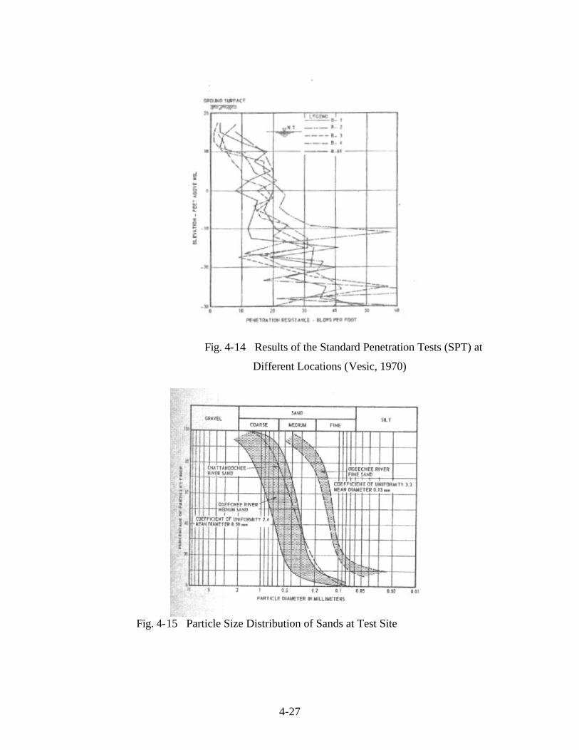
4-27
Fig. 4-14 Results of the Standard Penetration Tests (SPT) at
Different Locations (Vesic, 1970)
Fig. 4-15 Particle Size Distribution of Sands at Test Site

4-28
Fig. 4-16 A Comparison Between Measured and Computed Axial Pile
Load at Different Depths (After Vesic, 1970)
0 200 400 600 800Axial Pile Load, Q, Kips
20
10
0
Dep
th (f
t)
0 200 400 600 800
ComputedMeasured
0 200 400 600 800Axial Pile Load, Q, Kips
40
30
20
10
0
Dep
th (f
t)
0 200 400 600 800
ComputedMeasured
0 200 400 600 800Axial Pile Load, Q, Kips
50
40
30
20
10
0
Dep
th (f
t)
0 200 400 600 800
ComputedMeasured

5-1
CHAPTER 5
LATERAL LOADING OF A SHAFT IN LAYERED SOIL
USING THE STRAIN WEDGE MODEL
5.1 INTRODUCTION
The strain wedge (SW) model is an approach that has been developed to predict the response of a
flexible pile under lateral loading (Norris 1986, Ashour et al. 1996 and Ashour et al. 1998). The
main concept associated with the SW model is that traditional one-dimensional Beam on Elastic
Foundation (BEF) pile response parameters can be characterized in terms of three-dimensional
soil-pile interaction behavior. The SW model was initially established to analyze a free-head
pile embedded in one type of uniform soil (sand or clay). However, the SW model has been
improved and modified through additional research to accommodate a laterally loaded pile
embedded in multiple soil layers (sand and clay). The SW model has been further modified to
include the effect of pile head conditions on soil-pile behavior. The main objective behind the
development of the SW model is to solve the BEF problem of a laterally loaded pile based on the
envisioned soil-pile interaction and its dependence on both soil and pile properties.
The problem of a laterally loaded pile in layered soil has been solved by Reese (1977) as a BEF
based on modeling the soil response by p-y curves. However, as mentioned by Reese (1983), the
nonlinear p-y curve employed does not account for soil continuity and pile properties such as
pile stiffness, pile cross-section shape and pile head conditions.
The SW model was initially developed to assess the response of a laterally loaded long (slender)
pile (diameter < 3 ft). As a result, the effect of the vertical side shear (Vv) along the side of a
large diameter shaft should be integrated in the SW model analysis to account for such a
significant parameter in the analysis of large diameter shafts (Fig. 5-1). In addition, the
characterization of the intermediate and short shafts should be incorporated in the SW model
analysis to cover broader aspects of the shaft/pile analysis.

5-2
5.2 THE THEORETICAL BASIS OF STRAIN WEDGE MODEL
CHARACTERIZATION
The SW model parameters are related to an envisioned three-dimensional passive wedge of soil
developing in front of the pile. The basic purpose of the SW model is to relate stress-strain-
strength behavior of the soil in the wedge to one-dimensional BEF parameters. The SW model
is, therefore, able to provide a theoretical link between the more complex three-dimensional soil-
pile interaction and the simpler one-dimensional BEF characterization. The previously noted
correlation between the SW model response and BEF characterization reflects the following
interdependence:
• the horizontal soil strain (ε) in the developing passive wedge in front of the pile to the
deflection pattern (y versus depth, x) of the pile;
• the horizontal soil stress change (∆σh) in the developing passive wedge to the soil-pile
reaction (p) associated with BEF behavior; and
• the nonlinear variation in the Young's modulus (E = ∆σh/ε) of the soil to the nonlinear
variation in the modulus of soil subgrade reaction (Es = p/y) associated with BEF
characterization.
The analytical relations presented above reflect soil-pile interaction response characterized by
the SW model that will be illustrated later. The reason for linking the SW model to BEF analysis
is to allow the appropriate selection of BEF parameters to solve the following fourth-order
ordinary differential equation to proceed.
where MR is the resisting bending moment per unit length induced along the shaft length (x) due
to the vertical side shear (VV) (Fig. 5-1). The closed form solution of the basic form of the above
equation has been obtained by Matlock and Reese (1961) for the case of uniform soil. In order
to appreciate the SW model’s enhancement of BEF analysis, one should first consider the
governing analytical formulations related to the passive wedge in front of the shaft, the soil’s
0 =xd
Md +
x d
y d P +y (x) E + x d
y d EI R2
2
xs4
4
2
2
(5-1)

5-3
stress-strain and the vertical side shear (t-z curve) formulations, and the related soil-pile
interaction.
5.3 SOIL PASSIVE WEDGE CONFIGURATION
The SW model represents the mobilized passive wedge in front of the pile which is characterized
by base angles, ϕm and βm, the current passive wedge depth h, and the spread of the wedge fan
angle, ϕ m (the mobilized friction angle of soil). The horizontal stress change at the passive
wedge face, ∆σh, and side shear, τ, act as shown in Fig. 5-2. One of the main assumptions
associated with the SW model is that the deflection pattern of the pile is taken to be linear over
the controlling depth of the soil near the pile top resulting in a linearized deflection angle, δ, as
seen in Fig. 5-3.
The SW model makes the analysis simpler because forces (F1) on the opposite faces cancel, but
the real zone of stress is like the dashed outline shown in Fig. 5-4b which includes side shear
influence (ô) on the shape of the strained zone. However, the ô perpendicular to the face of the
pile is still considered in the SW model analysis. As seen in Fig. 5-4c, the horizontal equilibrium
in the SW wedge model is based on the concepts of the conventional triaxial test. The soil at the
face of the passive wedge is represented by a soil sample in the conventional triaxial test where
voσ (i.e. K = 1) and the horizontal stress change, Äóh, (from pile loading) are the confining and
deviatoric stresses in the triaxial test, respectively.
The relationship between the actual (closed form solution) and linearized deflection patterns of
long pile/shaft has been established by Norris (1986) (h/Xo = 0.69). As seen in 5-5, the
relationship (h/Xo) between the actual and linearized deflection for the short shaft is equal to 1,
and varies for the intermediate shafts from 0.69 at (L/T = 4) to 1 at (L/T = 2). As presented in
Chapter 2, L is the embedded length of the shaft and T is the initial relative shaft stiffness.
It should be noted that the idea of the change in the full passive wedge (mobilized passive wedge
at different levels of deflection) employed in the SW model has been shown experimentally by
Hughes and Goldsmith (1978) and previously established by Rowe (1956).

5-4
Changes in the shape and depth of the upper passive wedge, along with changes in the state of
loading and shaft/pile deflection, occur with change in the uniform strain (ε) in the developing
passive wedge. As seen in Fig. 5-6, two mobilized (tip to tip) passive wedges are developed in
soil in front of the short shaft. Because of the shaft straight-line deflection pattern with a
deflection angle δ, the uniform soil strain (ε) will be the same in both (i.e. upper and lower)
passive wedges.
As shown in Figs. 5-5 and 5-6, the deflection pattern is no longer a straight line for the
intermediate shaft, and the lower passive wedge has a curved shape that is similar to the
deflection pattern. Accordingly, the soil strain (εx) at depth x below the zero crossing will not be
uniform and will be evaluated in an iterative method based on the associated deflection at that
depth (Fig. 5-6c)
The lateral response of the short shaft is governed by both (upper and lower) developed passive
wedges (Fig. 5-6). However, with the intermediate shaft, less soil strain (i.e. stress on soil)
develops in the lower passive soil wedge (the inverted wedge below the point of zero crossing)
compared to the upper one (Fig. 5-6). The non-uniform soil strain (εx) in the lower passive soil
wedge (Fig. 5-6c) becomes much smaller compared to the strain in the upper soil wedge when
the shaft deflection approaches the deflection pattern of the long shaft. Since the lateral
deflection of the long pile/shaft below the zero crossing is always very small, the associated soil
strain and developing passive wedge will be very small as well. Consequently, the developing
upper passive soil wedge (and uniform strain therein) dominates the lateral response of the long
pile/shaft; hence the adopted name “strain wedge” (SW).
As seen in Figs. 5-3 and 5-6, the configuration of the wedge at any instant of load and,
therefore,base angle
mobilized friction angle, ϕm, and wedge depth, h, is given by the following equation:
or its complement
2 - 45 = m
m
ϕΘ (5-2)

5-5
The width, BC , of the wedge face at any depth is
ϕβmm
2 x) - h ( + D = BC tantan (5-4)
where x denotes the depth below the top of the studied passive wedge, and D symbolizes the
width of the pile cross-section. It should be noted that the SW model is based upon an effective
stress analysis of both sand and clay soils. As a result, the mobilized fanning angle, ϕm, is not
zero in clay soil as assumed by Reese (1958, 1983).
The above equations are applied to the upper and lower passive wedges in the case of short and
intermediate shafts where x for any point on the lower passive wedge (Fig. 5-6c) is measured
downward from the zero crossing and replaces the term (h - x) in Eqn. 5-4. Therefore,
)(/)/(δδ
εδεε xxx xy = = (5-5)
where ε and δ are the uniform soil strain and linearized shaft deflection angle of the upper
passive wedge, respectively. yx and δx are the shaft deflection and secant deflection angle at
depth x below the zero crossing (Fig. 5-6c).
5.4 STRAIN WEDGE MODEL IN LAYERED SOIL
The SW model can handle the problem of multiple soil layers of different types. The approach
employed, which is called the multi- sublayer technique, is based upon dividing the soil profile
and the loaded pile into sublayers and segments of constant thickness, respectively, as shown in
Fig. 5-7. Each sublayer of soil is considered to behave as a uniform soil and have its own
properties according to the sublayer location and soil type. In addition, the multi- sublayer
technique depends on the deflection pattern of the embedded pile being continuous regardless of
the variation of soil types. However, the depth, h, of the deflected portion of the pile is
controlled by the stability analysis of the pile under the conditions of soil-pile interaction. The
effects of the soil and pile properties are associated with the soil reaction along the pile by the
2 + 45 = m
m
ϕβ (5-3)

5-6
Young's modulus of the soil, the stress level in the soil, the pile deflection, and the modulus of
subgrade reaction between the pile segment and each soil sublayer. To account for the
interaction between the soil and the pile, the deflected part of the pile is considered to respond as
a continuous beam loaded with different short segments of uniform load and supported by
nonlinear elastic supports along soil sublayers, as shown in Fig. 5-8. At the same time, the point
of zero deflection (Xo in Fig. 5-5) for a pile in a particular layered soil varies according to the
applied load and the soil strain level.
The SW model in layered soil provides a means for distinguishing layers of different soil types
as well as sublayers within each layer where conditions (ε50, SL, ϕm) vary even though the soil
and its properties (γ, e or Dr, ϕ , etc.) remain the same. As shown in Fig. 5-9 , there may be
different soil layers and a transition in wedge shape from one layer to the next, with all
components of the compound wedge having in common the same depth h. In fact, there may be
a continuous change over a given sublayer; but the values of stress level (SL) and mobilized
friction angle (ϕm) at the middle of each sublayer of height, Hi, are treated as the values for the
entire sublayer.
As shown in Fig. 5-9, the geometry of the compound passive wedge depends on the properties
and the number of soil types in the soil profile, and the global equilibrium between the soil layers
and the loaded pile. An iterative process is performed to satisfy the equilibrium between the
mobilized geometry of the passive wedge of the layered soil and the deflected pattern of the pile
for any level of loading.
While the shape of the wedge in any soil layer depends upon the properties of that layer and,
therefore, satisfies the nature of a Winkler foundation of independent “soil” springs in BEF
analysis, realize that there is forced interdependence given that all components of the compound
wedge have the same depth (h) in common. Therefore, the mobilized depth (h) of the compound
wedge at any time is a function of the various soils (and their stress levels), the bending stiffness
(EI), and head fixity conditions (fixed, free, or other) of the pile. In fact, the developing depth of
the compound wedge can be thought of as a retaining wall of changing height, h. Therefore, the
resultant “soil” reaction, p, from any soil layer is really a “soil-pile” reaction that depends upon

5-7
the neighboring soil layers and the pile properties as they, in turn, influence the current depth, h.
In other words, the p-y response of a given soil layer is not unique. The governing equations of
the mobilized passive wedge shape are applied within each one- or two-foot sublayer i (of a
given soil layer I) and can be written as follows:
( ) ( )2
- 45 = m i
m i
ϕΘ (5-6)
( ) ( )2
+ 45 = m im i
ϕβ (5-7)
( ) ( ) ( ) 2 ) x - h ( + D = BC m im iiiϕβ tantan (5-8)
where h symbolizes the entire depth of the compound passive wedge in front of the pile and xi
represents the depth from the top of the pile or compound passive wedge to the middle of the
sublayer under consideration. Equations 5-6 through 5-8 are applied at the middle of each
sublayer. In the case of short and intermediate shafts, xi is measured downward from the point of
zero crossing and replaces the term (h - xi) in Eqn 5-8, as shown in Fig. 5-6, for analysis of the
lower wedge.
5.5 SOIL STRESS-STRAIN RELATIONSHIP
The horizontal strain (ε) in the soil in the passive wedge in front of the pile is the predominant
parameter in the SW model; hence, the name “strain wedge”. Consequently, the horizontal stress
change (∆σh) is constant across the width of the rectangle BCLM (of face width BC of the
passive wedge ), as shown in Fig. 5-4. The stress-strain relationship is defined based on the
results of the isotropically consolidated drained (sand) or undrained (clay) triaxial test. These
properties are summarized as follows:
• The major principle stress change (∆σh) in the wedge is in the direction of pile
movement, and it is equivalent to the deviatoric stress in the triaxial test as shown in Fig.
5-4 (assuming that the horizontal direction in the field is taken as the axial direction in the
triaxial test).
• The vertical stress change (∆σv) and the perpendicular horizontal stress change (∆σph)
equal zero, corresponding to the standard triaxial compression test where deviatoric stress

5-8
is increased while confining pressure remains constant.
• The initial horizontal effective stress is taken as
σσσ vovoho = K =
where K=1 due to pile installation effects. Therefore, the isotropic confining pressure in
the triaxial test is taken as the vertical effective stress (σvo) at the associated depth.
• The horizontal stress change in the direction of pile movement is related to the current
level of horizontal strain (ε) and the associated Young's modulus in the soil, as are the
deviatoric stress and the axial strain, to the secant Young’s modulus (E = ∆σh/ε) in the
triaxial test.
• Both the vertical strain (εv ) and the horizontal strain perpendicular to pile movement (εph)
are equal and are given as
εv = εph = -ν ε
where ν is the Poisson’s ratio of the soil.
It can be demonstrated from a Mohr’s circle of soil strain, as shown in Fig. 5-10, that shear
strain, γ, is defined as
( ) ( ) ΘΘ mmv 2 + 1 21
= 2 - 21
= 2
sinsin νεεεγ (5-9)
The corresponding stress level (SL) in sand (see Fig. 5-11) is
( )( ) 1 - + 45
1 - + 45 = = SL
2
m2
hf
h
2/tan
2/tanϕϕ
σσ
∆∆
(5-10)
where the horizontal stress change at failure (or the deviatoric stress at failure in the triaxial test)
is
∆ 1 -
2 + 45 = 2
vohf
ϕσσ tan (5-11)
5-9
In clay,
S 2 = ;
= SL uhfhf
h σσσ ∆
∆∆
(5.12)
where Su represents the undrained shear strength which may vary with depth. Determination of
the values of SL and ϕm in clay requires the involvement of an effective stress analysis which is
presented later in this chapter.
The relationships above show clearly that the passive wedge response and configuration change
with the change of the mobilized friction angle (ϕm) or stress level (SL) in the soil. Such
behavior provides the flexibility and the accuracy for the strain wedge model to accommodate
both small and large strain cases. The above equations are applied for each soil sublayer along
the shaft in order to evaluate the varying stress level in the soil and the geometry of the passive
wedges.
A power function stress-strain relationship is employed in SW model analysis for both sand and
clay soils. It reflects the nonlinear variation in stress level (SL) with axial strain (ε) for the
condition of constant confining pressure. To be applicable over the entire range of soil strain, it
takes on a form that varies in stages as shown in Fig. 5-12. The advantage of this technique is
that it allows the three stages of horizontal stress, described in the next section, to occur
simultaneously in different sublayers within the passive wedge.
5.5.1 Horizontal Stress Level (SL)
Stage I (εε ≤≤ εε 50% )
The relationship between stress level and strain at each sublayer (i) in the first stage is assessed
using the following equation,
( ) ) SL 3.707- (
= SL i
50 i
ii exp
εελ (5.13)
where 3.707 and λ ( λ= 3.19) represent the fitting parameters of the power function relationship,
and ε50 symbolizes the soil strain at 50 percent stress level at the associated confining pressure.

5-10
Stage II ( εε 50% ≤≤ εε ≤≤ εε 80 % )
In the second stage of the stress-strain relationship, Eqn. 5.13 is still applicable. However, the
value of the fitting parameter λ is taken to vary in a linear manner with SL from 3.19 at the 50
percent stress level to 2.14 at the 80 percent stress level as shown in Fig. 5-12b.
Stage III ( εε ≥≥ εε 80% )
This stage represents the final loading zone which extends from 80 percent to 100 percent stress
level. The following equation is used to assess the stress-strain relationship in this range,
( ) 0.80 SL q + m
100 + 0.2 = SL i
ii
ii ≥
;lnexp
εε
(5-14)
where m=59.0 and q=95.4 ε50 are the required values of the fitting parameters.
The three stages mentioned above are developed based on unpublished experimental results
(Norris 1977). In addition, the continuity of the stress-strain relationship is maintained along the
SL-ε curve at the merging points between the mentioned stages.
As shown in Fig. 5-13, if ε50 of the soil is constant with depth (x), then, for a given horizontal
strain (ε), SL from Eqns 5-13 or 5-14 will be constant with x. On the other hand, since strength,
∆σhf, varies with depth (e.g., see Eqns. 5-11 and 5-12), ∆σh (= SL ∆σhf ) will vary in a like
fashion. However, ε50 is affected by confining pressure (σvo) in sand and Su in clay. Therefore,
SL for a given ε will vary somewhat with depth.
The Young’s modulus of the soil from both the shear loading phase of the triaxial test and the
strain wedge model is
( ) ( )εσ
εσ
SL =
= Ehf iih i
i
∆∆ (5.15)

5-11
It can be seen from the previous equations that stress level, strain and Young's modulus at each
sublayer (i) depend on each other, which results in the need for an iterative solution technique to
satisfy the equilibrium between the three variables.
5.6 SHEAR STRESS ALONG THE PILE SIDES (SLt)
Shear stress (τ) along the pile sides in the SW model (see Fig. 5-4) is defined according to the
soil type (sand or clay).
5.6.1 Pile Side Shear in Sand
In the case of sand, the shear stress along the pile sides depends on the effective stress (σvo) at the
depth in question and the mobilized angle of friction between the sand and the pile (ϕs). The
mobilized side shear depends on the stress level and is given by the following equation,
( ) ( ) ( ) 2 = where ; ) ( = m is is iivoi ϕϕϕστ tantantan (5-16)
In Eqn. 5-16, note that mobilized side shear angle, tanϕs, is taken to develop at twice the rate of
the mobilized friction angle (tanϕm) in the mobilized wedge. Of course, ϕs is limited to the fully
developed friction angle (ϕ) of the soil.
5.6.2 Pile Side Shear Stress in Clay
The shear stress along the pile sides in clay depends on the clay’s undrained shear strength. The
stress level of shear along the pile sides (SLt) differs from that in the wedge in front of the pile.
The side shear stress level is function of the shear movement, equal to the pile deflection (y) at
depth x from the ground surface. This implies a connection between the stress level (SL) in the
wedge and the pile side shear stress level (SLt). Using the Coyle-Reese (1966) “t-z” shear stress
transfer curves (Fig. 5-14), values for SLt can be determined. The shear stress transfer curves
represent the relationship between the shear stress level experienced by a one-foot diameter pile
embedded in clay with a peak undrained strength, Su, and side resistance, τult (equal to ζ times
the adhesional strength αSu), for shear movement, y. The shear stress load transfer curves of
Coyle-Reese can be normalized by dividing curve A (0 < x < 3 m) by ζ = 0.53, curve B (3 < x <
5-12
6 m) by ζ = 0.85, and curve C ( x > 6 m) by ζ = 1.0. These three values of normalization (0.53,
0.85, 1.0) represent the peaks of the curves A, B, and C, respectively, in Fig. 5-15a. Figure 5-
15b shows the resultant normalized curves. Knowing pile deflection (y), one can assess the
value of the mobilized pile side shear stress (τ) as
( ) ( ) SL = ult it ii ττ (5-17)
where
) S = ) ( iuiult αζτ ( (5-18)
and α indicates the adhesion value after Tomlinson (1957).
The normalized shear stress load transfer curves can be represented by the following equations.
For the normalized curves A (x < 3 m) and B (3 < x < 6 m),
D y 40.5 - Dy 12.9 = SL 22t (5-19)
For the normalized curve C (x > 6 m)
D y 255 - Dy 32.3 = SL 22t (5-20)
where y is in cm and D in m.
From the discussion above, it is obvious that SLt varies nonlinearly with the pile deflection, y, at
a given soil depth, x. Also, SLt changes nonlinearly with soil depth for a given value of soil
displacement/strain (see Fig. 5-15). These concepts are employed in each sublayer of clay.
5.7 SOIL PROPERTY CHARACTERIZATION IN THE STRAIN WEDGE MODEL
One of the main advantages of the SW model approach is the simplicity of the required soil
properties necessary to analyze the problem of a laterally loaded pile. The properties required
represent the basic and the most common properties of soil, such as the effective unit weight and
the angle of internal friction or undrained strength.

5-13
The soil profile is divided into one or two foot sublayers, and each sublayer is treated as an
independent entity with its own properties. In this fashion, the variation in soil properties or
response (such as ε50 and ϕ in the case of sand, or Su and ϕ in the case of clay) at each sublayer
of soil can be explored. It is obvious that soil properties should not be averaged at the midheight
of the passive wedge in front of the pile for a uniform soil profile (as in the earlier work of Norris
1986), or averaged for all sublayers of a single uniform soil layer of a multiple layer soil profile.
5.7.1 Propert ies Employed for Sand Soil
• Effective unit weight (total above water table, buoyant below), γ
• Void ratio, e, or relative density, Dr
• Angle of internal friction, ϕ
• Soil strain at 50% stress level, ε50
While standard subsurface exploration techniques and available correlations may be used to
evaluate or estimate γ , e or Dr, and ϕ, some guidance may be required to assess ε50.
The ε50 represents the axial strain (ε1 ) at a stress level equal to 50 percent in the ε1-SL
relationship that would result from a standard drained (CD) triaxial test. The confining
(consolidation) pressure for such tests should reflect the effective overburden pressure (σvo) at
the depth (x) of interest. The ε50 changes from one sand to another and also changes with density
state. In order to obtain ε50 for a particular sand, one can use the group of curves shown in Fig.
5-16 (Norris 1986) which show a variation based upon the uniformity coefficient, Cu, and void
ratio, e. These curves have been assessed from sand samples tested with “frictionless” ends in
CD tests at a confining pressure equal to 42.5 kPa (Norris 1977). Since the confining pressure
changes with soil depth, ε50, as obtained from Fig. 5-16, should be modified to match the existing
pressure as follows:
( ) ( )
42.5
) ( = vo i
0.2
42.55050 i
σεε (5-21)

5-14
( ) ( )
∆ 1 -
2 + 45 = i2
vo ihf i
ϕσσ tan (5-22)
where σvo should be in kPa.
5.7.2 The Properties Employed for Clay
• Effective unit weight γ
• Plasticity index, PI
• Effective angle of friction, ϕ
• Undrained shear strength, Su
• Soil strain at 50% stress level, ε50
Plasticity index, PI, and undrained shear strength, Su, are considered the governing properties
because the effective angle of internal friction, ϕ, can be estimated from the PI based on Fig. 5-
17. The ε50 from an undrained triaxial test (UU at depth x or CU with σ3 =σvo) can be
estimated based on Su as indicated in Fig. 5-18.
An effective stress (ES) analysis is employed with clay soil as well as with sand soil. The reason
behind using the ES analysis with clay, which includes the development of excess porewater
pressure with undrained loading, is to define the three-dimensional strain wedge geometry based
upon the more appropriate effective stress friction angle,ϕ. The relationship between the
normally consolidated clay undrained shear strength, Su, and σvo is taken as
σvou 0.33 = S (5-23)
assuming that Su is the equivalent undrained standard triaxial test strength. The effective stress
analysis relies upon the evaluation of the developing excess porewater pressure based upon
Skempton's equation (1954), i.e.
( )[ ] - A + B = u 31u3 σσσ ∆∆∆∆ (5-24)

5-15
where B equals 1 for saturated soil. Accordingly,
( ) - A + = u 31u3 σσσ ∆∆∆∆ (5-25)
Note that ∆σ3 =0 both in the shear phase of the triaxial test and in the strain wedge. Therefore,
the mobilized excess porewater pressure is
σ1u A = u ∆∆ (5-26)
where ∆σ1 represents the deviatoric stress change in the triaxial test and ∆σh in the field, i.e.
σhu A = u ∆∆ (5-27)
Therefore, using the previous relationships, the Skempton equation can be rewritten for any
sublayer (i) as follows:
) S ( 2 SL ) A ( = ) ( SL ) A ( = ) u (iuiiuihfiiui σ∆∆ (5-28)
The initial value of parameter Au is 0.333 and occurs at very small strain for elastic soil response.
In addition, the value of parameter Auf that occurs at failure at any sublayer (i) is given by the
following relationship
1 -
) (
)S(1 + 1
2
1 = ) A (
iivo
iu
iufϕσ sin
/(5-29)
after Wu (1966) as indicated in Fig. 5-19.
In Eqn. 5.29, ϕ symbolizes the effective stress angle of internal friction; and, based on Eqn. 5-
23, Su/σvo equals 0.33. However, Au is taken to change with stress level in a linear fashion as
[ ] 0.333 - ) A ( SL + 0.333 = ) A (iufiiu (5-30)

5-16
By evaluating the value of Au, one can effectively calculate the excess porewater pressure, and
then can determine the value of the effective horizontal stress, (σ–vo + ∆σh - ∆u), and the effective
confining pressure, (σ–vo - ∆u) at each sublayer, as shown in Fig. 5-19. Note that the mobilized
effective stress friction angle, ϕ–m, can be obtained from the following relationship.
( )( )u -
u - + =
2
) ( + 45
vo i
hvo iim2
∆∆∆
σσσϕ
tan (5-31)
The targeted values of ϕmi and SLi in a clay sublayer and at a particular level of strain (ε) can be
obtained by using an iterative solution that includes Eqns 5-12 through 5-14, and 5-28 through 5-
31.
5.8 SOIL-PILE INTERACTION IN THE STRAIN WEDGE MODEL
The strain wedge model relies on calculating the modulus of subgrade reaction, Es, which
reflects the soil-pile interaction at any level of soil strain during pile loading. Es also represents
the secant slope at any point on the p-y curve, i.e.
y
p = E s (5-32)
Note that p represents the force per unit length of the pile or the BEF soil-pile reaction, and y
symbolizes the pile deflection at that soil depth. In the SW model, Es is related to the soil’s
Young's modulus, E, by two linking parameters, A and ψs. It should be mentioned here that the
SW model establishes its own Es from the Young's modulus of the strained soil, and therefore,
one can assess the p-y curve using the strain wedge model analysis. Therefore, Es should first be
calculated using the strain wedge model analysis to identify the p and y values.
Corresponding to the horizontal slice (a soil sublayer) of the passive wedge at depth x (see Figs.
5-2 and 5-4), the horizontal equilibrium of horizontal and shear stresses is expressed as
( ) S D 2 + S BC = p 2i1ih ii τσ∆ (5-33)

5-17
where S1 and S2 equal to 0.75 and 0.5, respectively, for a circular pile cross section, and equal to
1.0 each for a square pile (Briaud et al. 1984). Alternatively, one can write the above equation as
follows:
( ) ( ) S 2
+ D
S BC =
D p = A
h i
2i1i
h i
ii
στ
σ ∆∆/
(5-34)
where A symbolizes the ratio between the equivalent pile face stress, p/D, and the horizontal
stress change, ∆σh, in the soil. (In essence, it is the multiplier that, when taken times the
horizontal stress change, gives the equivalent face stress.) From a different perspective, it
represents a normalized width (that includes side shear and shape effects) that, when multiplied
by ∆σh yields p/D. By combining the equations of the passive wedge geometry and the stress
level with the above relationship, one finds that
( ) ( ) ( ) ( )( ) sandin
S 2 +
D
2 x - h + 1 S = A
h i
s ivo i2mm ii1i
σ
φσϕβ∆
tantantan(5-35)
( ) ( ) ( )clay in
SL
SL S + D
2 x - h + 1 S = A
i
t i2mm ii1i
ϕβ tantan(5-36)
Here the parameter A is a function of pile and wedge dimensions, applied stresses, and soil
properties. However, given that ∆σh = Eε in Eqn. 2.33,
εσ E D A = ) ( D A = p iiihii∆ (5-37)
For the upper passive wedge, ε represents the uniform soil strain and is replaced by εx for soil
sublayers of the lower passive wedge. The second linking parameter, Ψs, relates the soil strain in
the SW model to the linearized pile deflection angle, δ. Referring to the normalized pile
deflection shape shown in Figs. 5-3 and 5-5
2 = γδ (5-38)

5-18
Θm 2 2
= 2
sinmaxγγ(5-39)
and
( )2
+ 1 =
2 -
= 2
v ενεεγmax (5-40)
where γ denotes the shear strain in the developing passive wedge. Using Eqns. 5-39 and 5.40,
Eqn. 5-38 can be rewritten as
( )2
2 + 1 = mΘsinνεδ (5-41)
Based on Eqn. 5-41, the relationship between ε and δ can expressed as
δε
= Ψ (5-42)
or
( ) ΘΨ
m 2 + 1
2 =
sinν(5-43)
The parameter ψ varies with the Poisson's ratio of the soil and the soil's mobilized angle of
internal friction (ϕm) and the mobilized passive wedge angle (Θm).
Poisson's ratio for sand can vary from 0.1 at a very small strain to 0.5 or lager (due to dilatancy)
at failure, while the base angle, Θm, can vary between 45o (for ϕm = 0 at ε= 0) and 25o (for, say,
ϕm = 40o at failure), respectively. For this range in variation for ν and ϕm, the parameter Ψ for
sand varies between 1.81 and 1.74 with an average value of 1.77. In clay soil, Poisson's ratio is
assumed to be 0.5 (undrained behavior) and the value of the passive wedge base angle, Θm, can
vary between 45o (for ϕm = 0 at ε = 0) and 32.5o (for, say, ϕm = 25o at failure). Therefore, the
value of the parameter ψ will vary from 1.47 to 1.33, with an average value of 1.4.
It is clear from the equations above that employing the multi- sublayer technique greatly
influences the values of soil-pile interaction as characterized by the parameter, Ai, which is

5-19
affected by the changing effective stress and soil strength from one sublayer to another. The
final form of the modulus of subgrade reaction can be expressed as
( ) ( ) ( ) E D x - h
A = x - h
E D A = y
p = E i
i
i
i
ii
i
is i Ψ
δε
(5-44)
It should be mentioned that the SW model develops its own set of non-unique p-y curves which
are function of both soil and pile properties, and are affected by soil continuity (layering) as
presented by Ashour et al. (1996). For the lower passive wedge, (h – xi) will be replaced by xi
that is measured downward from the point of zero crossing (Fig. 5-6).
5.9 PILE HEAD DEFLECTION
As mentioned previously, the deflection pattern of the pile in the SW model is continuous and
linear. Based on this concept, pile deflection can be assessed using a simplified technique which
provides an estimation for the linearized pile deflection, especially yo at the pile head. By using
the multi-sublayer technique, the deflection of the pile can be calculated starting with the base of
the mobilized passive wedge and moving upward along the pile, accumulating the deflection
values at each sublayer as shown in the following relationships and Fig. 5-20.
s
iiii H = H = yΨε
δ (5-45)
n to 1 =i y = yio
Σ (5-46)
where the ψs value changes according to the soil type (sand or clay), and Hi indicates the
thickness of sublayer i and n symbolizes the current number of sublayers in the mobilized
passive wedge.
The main point of interest is the pile head deflection which is a function of not only the soil
strain but also of the depth of the compound passive wedge that varies with soil and pile
properties and the level of soil strain.
5.10 ULTIMATE RESISTANCE CRITERIA IN STRAIN WEDGE MODEL

5-20
The mobilized passive wedge in front of a laterally loaded pile is limited by certain constraint
criteria in the SW model analysis. Those criteria differ from one soil to another and are applied
to each sublayer. Ultimate resistance criteria govern the shape and the load capacity of the
wedge in any sublayer in SW model analysis. The progressive development of the ultimate
resistance with depth is difficult to implement without employing the multi- sublayer technique.
5.10.1 Ultimate Resistance Criterion of Sand Soil
The mobilization of the passive wedge in sand soil depends on the horizontal stress level, SL,
and the pile side shear resistance, τ. The side shear stress is a function of the mobilized side
shear friction angle, ϕs, as mentioned previously, and reaches its ultimate value (ϕs = ϕ) earlier
than the mobilized friction angle, ϕm, in the wedge (i.e. SLt ≥ SL). This causes a decrease in the
rate of growth of sand resistance and the fanning of the passive wedge as characterized by the
second term in Eqns 5-33 and 5-35, respectively.
Once the stress level in the soil of a sublayer of the wedge reaches unity (SLi = 1), the stress
change and wedge fan angle in that sublayer cease to grow. However, the width BC of the face
of the wedge can continue to increase as long as ε (and, therefore, h in Eqn. 5-8) increases.
Consequently, soil-pile resistance, p, will continue to grow more slowly until a condition of
initial soil failure (SLi = 1) develops in that sublayer. At this instance, p = pult where pult in sand,
given as
( ) ( ) ( ) S D 2 + S BC = p 2f i1ihf iult i τσ∆ (5.47)
pult is “a temporary” ultimate condition, i.e. the fanning angle of the sublayer is fixed and equal
to ϕi, but the depth of the passive wedge and, hence, BC continue to grow. The formulation
above reflects that the near-surface “failure” wedge does not stop growing when all such
sublayers reach their ultimate resistance at SL = 1 because the value of h at this time is not
limited. Additional load applied at the pile head will merely cause the point at zero deflection
and, therefore, h to move down the pile. More soil at full strength (SL = 1) will be mobilized to

5-21
the deepening wedge as BC, therefore, pult will increase until either flow around failure or a
plastic hinge in the pile occurs.
Recognize that flow around failure occurs in any sublayer when it is easier for the sand at that
depth to flow around the pile in a local bearing capacity failure than for additional sand to be
brought to failure and added to the already developed wedge. However, the value at which flow
failure occurs [Ai = (Ault)i , (pult)i = (∆σhf)i (Ault)i D] in sand is so large that it is not discussed
here. Alternatively, a plastic hinge can develop in the pile when the pile material reaches its
ultimate resistance at a time when SLi ≤ 1 and Ai < (Ault)i. In this case, h becomes fixed, and BCi
and pi will be limited when SLi becomes equal to 1.
5.10.2 Ultimate Resistance Criterion of Clay Soil
The situation in clay soil differs from that in sand and is given by Gowda (1991) as a function of
the undrained strength (Su)i of the clay sublayer.
( ) ( ) ( ) S D S 2 + S D S 10 = p 2u i1u iult i(5-48)
Consequently,
( )( )
( )( )
( ) S + S5 = S 2 D
p =
D
p
= A 21u i
ult i
hf i
ult i
ult i σ∆(5-49)
Ault indicates the limited development of the sublayer wedge geometry for eventual development
of flow around failure (SLi = 1) and, consequently, the maximum fanning angle in that sublayer
becomes fixed, possibly at a value ϕm ≤ ϕ. If a plastic hinge develops in the pile at SLi less
than 1, then h will be limited, but BC, and pi will continue to grow until Ai is equal to Ault or pi is
equal to (pult)i.

5-22
5.11 VERTICAL SIDE SHEAR RESISTANCE
As seen in Fig. 5-21, the vertical side shear stress distribution around the shaft cross section is
assumed to follow a cosine function. It is assumed that there is no contact (active pressure) on
the backside of the shaft due to the lateral deflection. The peak (q) of side shear stress develops
at angle θ = 0 and decreases to zero at angle θ = 90o. The total vertical side shear force (Vv)
induced along a unit length of the shaft is expressed as
qDrqdrqVv === ∫ 2/0
2/
0)sin(2cos2 ππ
θθθ (5-50)
and the induced moment (Mx-x) per unit length of the shaft is given as
82(sin
2
1
)12(cos
)12(cos2
12
cos2)cos()cos(2
22/
0
2
2/
0
2
2/
0
2
2/
0
222/
0
πθθ
θθ
θθ
θθθθθ
π
π
π
ππ
Dqrq
drq
drq
drqrdrqM xx
=
+=
+=
+=
==
∫
∫
∫∫−
(5-51)
Mx-x represents the term MR in Eqn. 5-1.
5.12 SHAFT BASE RESISTANCE
The soil shear resistance at the base of the shaft (Vb) that is shown in Fig. 5-1 is a function of the
soil shear stress (τb) induced at the contact surface between the soil and shaft base. The shear
stress (τb) varies with lateral deflection of the shaft base and the axial load delivered at the shaft
base. Based on the failure mechanism at the shaft base for sand and clay that are presented in
Chapter 3 and 4, Fig. 5-22 shows the shear tress (τb) that develops at the shaft base embedded in
sand or clay soil. Unlike the clay case, the ultimate shear resistance at the base of the shaft
increases with the axial load carried by the shaft base (Figs. 4-1 and 5-22).

5-23
The shear resistance at the shaft base can be determined as follows,
1. Using the lateral deflection at the shaft base (yb) that is obtained from the lateral shaft
analysis with no shaft base resistance, the soil shear strain at the base (γb) is calculated as,
D
ybb
2=γ (5-52)
where D is the shaft diameter, and the effective depth of the shear deformation is
assumed to be equal to 2D
2. In the first step of analysis, assume the normal strain (εb) equal to the shear strain (γb).
Based on the normal stress strain relationship presented in Section 5.5.1, the stress level
(SL) can be evaluated and the associated Poisson’s ratio (ν) is calculated as follows,
SL4.01.0 +=ν (5-53)
It should be noted the ∆σhf used in Eqns. 5-10 through 5-12 is constant with clay (∆σhf =
2Su) and varies with the load carried by the shaft base in the case of sand (Figs. 4-1 and
5-22), i.e.
∆ 1 -
2 + 45 = 2
IVhf
ϕσσ tan)(
3(5-54)
In sand soil, the increase of the shaft base load (Fb = 0.6 qnet Ab = σd Ab = SL ∆σhf Ab)
results in the increase of the accompanying confining pressure IV )(3σ .
3. The induced normal strain (εb) is recalculated as follows,
)1( νγε+
= bb (5-55)
4. Repeat steps 2 and 3 to refine the value of εb by averaging the new and old values of εb
until reaching the desired convergence.
5. Compute the associated soil shear stress that develops on the shaft base (τb) as follows:

5-24
ub SSL=τ (Clay) (5-56a)
hfb SL στ ∆= 5.0 (Sand) (5-56b)
bbb AV τ= (5-57)
where Fb and Vb are the axial load (as calculated in Chapter 4) and the shear resistance
carried by the shaft base.
6. Analyze the laterally loaded shaft as a Beam on Elastic Foundations (Section 5-13)
considering the effect of the base resistance. The base shear resistance is evaluated in
each trial according to the lateral deflection induced at the shaft base.
5.13 STABILITY ANALYSIS IN THE STRAIN WEDGE MODEL
The objective of the SW model is to establish the soil response as well as model the soil-pile
interaction through the modulus of subgrade reaction, Es. The shape and the dimensions of the
passive wedge in front of the pile basically depend on two types of stability which are the local
stability of the soil sublayer and the global stability of the pile and the passive wedge. However,
the global stability of the passive wedge depends, in turn, on the local stability of the soil
sublayers.
5.13.1 Local Stability of a Soil Sublayer in the Strain Wedge Model
The local stability analysis in the strain wedge model satisfies equilibrium and compatibility
among the pile segment deflection, soil strain, and soil resistance for the soil sublayer under
consideration. Such analysis allows the correct development of the actual horizontal stress
change, ∆σh , pile side shear stress, τ, and soil-pile reaction, p, associated with that soil sublayer
(see Figs. 5-2 and 5-4). It is obvious that the key parameters of local stability analysis are soil
strain, soil properties, and pile properties.
5.13.2 Global Stability in the Strain Wedge Model
The global stability, as analyzed by the strain wedge model, satisfies the general compatibility
among soil reaction, pile deformations, and pile stiffness along the entire depth of the developing
passive wedge in front of the pile. Therefore, the depth of the passive wedge depends on the

5-25
global equilibrium between the loaded pile and the developed passive wedge. This requires a
solution for Eqn. 5-1.
The global stability is an iterative beam on elastic foundation (BEF) problem that determines the
correct dimensions of the passive wedge, the corresponding straining actions (deflection, slope,
moment, and shear) in the pile, and the external loads on the pile. Satisfying global stability
conditions is the purpose of linking the three-dimensional strain wedge model to the BEF
approach. The major parameters in the global pile stability problem are pile stiffness, EI, and the
modulus of subgrade reaction profile, Es, as determined from local stability in the strain wedge
analysis. Since these parameters are determined for the applied soil strain, the stability problem
is no longer a soil interaction problem but a one-dimensional BEF problem. Any available
numerical technique, such as the finite element or the finite difference method, can be employed
to solve the global stability problem. The modeled problem, shown in Fig. 5-8c, is a BEF and
can be solved to identify the depth, Xo, of zero pile deflection.
5.14 SUMMARY
The SW model approach presented here provides an effective method for solving the problem of
a laterally loaded pile/shaft in layered soil. This approach assesses its own nonlinear variation in
modulus of subgrade reaction or p-y curves. The SW model allows the assessment of the
nonlinear p-y curve response of a laterally loaded pile based on the envisioned relationship
between the three-dimensional response of a flexible pile in the soil to its one-dimensional beam
on elastic foundation parameters. In addition, the SW model employs stress-strain-strength
behavior of the soil as established from the triaxial test in an effective stress analysis to evaluate
mobilized soil behavior.
The SW model accounts for the vertical side shear resistance that develops effectively with large
diameter shafts. Such resistance enhances the performance of the large diameter shafts and
increases with progressive lateral deflection. The evaluation of the vertical side shear resistance
is based on the assessed t-z curve and affects the shape of the predicted p-y curve. The
formulations of the t-z curve presented in Chapters 3 and 4 are employed in the SW model
analysis and coupled with the shaft deformations.

5-26
Compared to empirically based approaches which rely upon a limited number of field tests, the
SW approach depends on well known or accepted principles of soil mechanics (the stress-strain-
strength relationship) in conjunction with effective stress analysis. Moreover, the required
parameters to solve the problem of the laterally loaded pile are a function of basic soil properties
that are typically available to the designer.

5-27
Fig. 5-1 Characterization of Large Diameter Long, Intermediate or Short Shafts
In Terms of a) Forces and b) Nonlinear Springs
Po
Mo
Vb
Fb
Vv
Vv
FP
FP
FP
Vh
Vh
Vh
Mb
Po
Mo
PV PV
FP
FP
FP
Fv
Fv
Fv
Fb
Mb
Vb
MR
MR
MR
(a) (b)

5-28
Fig. 5-2 The Basic Strain Wedge in Uniform Soil

5-29
Fig. 5-3 Deflection Pattern of a Laterally Loaded Long
Shaft/Pile and the Associated Strain Wedge
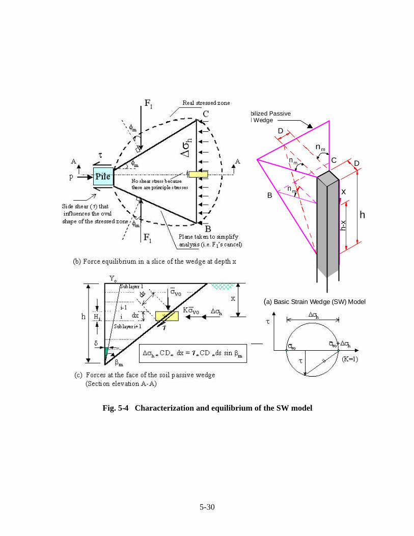
5-30
Fig. 5-4 Characterization and equilibrium of the SW model
Mobilized PassiveSoil Wedge
x
h
h-x
D
B
C
D
(a) Basic Strain Wedge (SW) Model
nm
nm
nm

5-31
Fig
. 5-5
D
efle
ctio
n P
atte
rns
of L
ong,
Int
erm
edia
te a
nd S
hort
Sha
fts
h = 0.69 Xo
Xo
Zer
o C
ross
ing
Xo > h > 0.69 Xo
Xo
Zer
o C
ross
ing
Zer
o C
ross
ing
h = Xo
Deflect
ion Pattern
Lineariz
ed D
eflec
tion
Yo
Yo
Yo
δδ
δ
Linearize
d Defl
ection
Deflectio
n Pattern
Lon
g S
haf
tL
/T ≥≥
4
Inte
rmed
iate
Sh
aft
4 >
L/T
> 2
Sh
ort
Sh
aft
L/T
≤≤ 2
δ

5-32
Fig. 5-6 Developed Passive Wedges with Short and Intermediate Shafts
Yo
b) Passive Wedges Developed with Short Shaft
βm
βm
Upper Passive Wedge
Lower Passive Wedge
Yo
δ
Strain Wedge(Side View)
Lower Passive Wedge
Upper Passive Wedge
Xo
>
h
>
0. 6
9
Xo
Xo
xh
=
L
-
Xo x
Zero Crossing
h
=
L
-
Xo Zero Crossing
x
h
=
Xo δ
xD
efle
ctio
n Pa
ttern
Def
lect
ion
Pat
tern
b) Passive Wedges Developed with Intermediate Shaft xn
xn+1
xn+2
xn+3
δn+1
δn+2
Zero Crossing
c) Varying Soil Strain and Deflection Angle in the Lower Passive Wedge
Def
lect
ion
Patte
rn
yn+3
yn+2

5-33
Fig. 5-7 The Linearized Deflection Pattern of a Pile/shaft Embedded in Soil Using theMulti Sublayer Strain Wedge Model

5-34
Fig. 5-8 Soil-Pile Interaction in the Multi-Sublayer Technique

5-35
Fig. 5-9 The Proposed Geometry of the Compound Passive Wedge

5-36
Fig
. 5-1
0 D
isto
rtio
n o
f th
e W
edge
a),
Th
e A
ssoc
iate
d M
ohr
Cir
cle
of S
trai
n b
), a
ndth
e R
elat
ions
hip
Bet
wee
n P
ile D
efle
ctio
n an
d W
edge
Dis
tort
ion
c)

5-35
Fig. 5-11 Relationship Between Horizontal Stress Change, Stress Level,
and Mobilized Friction Angle

5-36
Fig. 5-12 The Developed Stress-Strain Relationship in Soil

5-37
Fig. 5-13 The Nonlinear Variation of Stress Level Along
the Depth of Soil at Constant Strain

5-38
Fig. 5-14 The Employed Side Shear Stress-Displacement Curve in Clay

5-39
Fig. 5-15. The Nonlinear Variation of Shear Stress Level (SLt) with depth in Clay

5-40
Fig. 5-16 Relationship Between εε 50, Uniformity Coefficient (Cu) and Void Ratio (e) (Norris 1986)
0 0.25 0.5 0.75 1 1.25 1.5
Void Ratio, e
0
0.25
0.5
0.75
1
1.25
1.5
g 50
(%)
Uniformity Coefficient, Cu
1.182610

5-41
Fig. 5-17 Relationship Between Plasticity Index (PI) and Effective Stress Friction
Angle (ϕϕ ) (US Army Corps of Engineers 1996)

5-42
Fig. 5-18 Relationship Between �50 and Undrained Shear Strength , Su
(Evans and Duncan 1982)
50
u
0.00 0.01 0.02
g
100
1000
10000
200.00
300.00
500.00
2000.00
3000.00
5000.00
S
(psf
) Range of Suggested Values
(After Reese 1980)

5-43
Fig. 5-19 Relationship Between Effective Stress and Total Stress Conditions
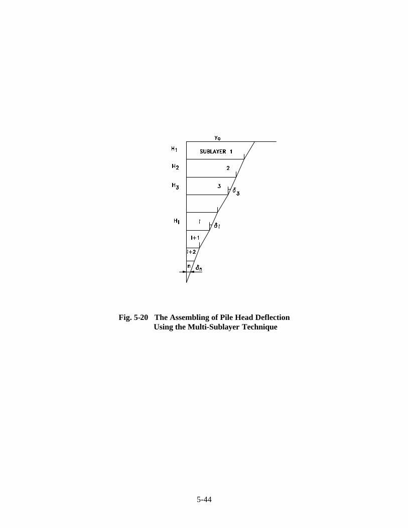
5-44
Fig. 5-20 The Assembling of Pile Head DeflectionUsing the Multi-Sublayer Technique

5-45
Fig. 5-21 Vertical Side Shear Stress Distribution on the Shaft Cross Section
Loading Direction θθ q
X
X
Shear Stress distribution
Shaft Cross Section

5-46
Fig. 5-22 Mobilized Shear Resistance at the Shaft Base in Sand and Clay
σ3 σ1σvo =σ
τ
τb
τult = c
Failure Envelop
Mobilized Envelop
(σ3)IV (σ3)IV = qultσvo
ϕI
ϕIV
qnet
σd= 0.6 q
net
Zone IVZone I σ
τ
ττb
Sand
Clay

6-1
CHAPTER 6
SHAFTS IN LIQUEFIABLE SOILS
6.1 INTRODUCTION
This chapter presents the procedure developed to assess the response of the partially and completely
liquefied granular soil as a post-liquefaction analysis. The SW model, initially developed to assess the
relationship between one-dimensional beam on elastic foundation (BEF) or so called “p-y” curve behavior
and three dimensional soil pile interaction, has been extended to include laterally loaded piles/shafts in
liquefiable soil. Because the SW model relies on the undrained stress-strain characterization of the soil as
occurs in the triaxial test, it is capable of treating one or more layers of soils that experience limited or full
liquefaction. This chapter provides a methodology to assess the post-liquefaction response of an isolated
pile/shaft in sand under an applied pile/shaft head load/moment combination assuming undrained conditions
in the sand. The degradation in soil strength due to the free-field excess porewater (uxs,ff), generated by the
earthquake that results in developing or full liquefaction, is considered along with the near-field excess
porewater pressure (uxs, nf) generated by lateral loading from the superstructure.
Current design procedures assume slight or no resistance for the lateral movement of the pile in the liquefied
soil which is a conservative practice. Alternatively, if liquefaction is assessed not to occur, some
practitioners take no account of the increased uxs,ff, and none consider the additional uxs, nf due to inertial
interaction loading from the superstructure; a practice that is unsafe in loose sands. The paper characterizes
the reduction in pile response and the changes in the associated p-y curves due to a drop in sand strength
and Young’s modulus as a result of developing liquefaction in the sand followed by inertial interaction
loading from the superstructure.
The potential of soil to liquefy is one of the critical research topics of the last few decades. Several studies
and experimental tests have been conducted for better understanding on the potential of soil to liquefy in
both the free- and/or near-field soil regions. However, predicting the response of pile foundations in

6-2
liquefied soil or soil approaching liquefaction is very complex.
The procedure presented predicts the post-liquefaction behavior of laterally loaded piles in sand under
developing or fully liquefied conditions. Due to the shaking from the earthquake and the associated lateral
load from the superstructure, the free field uxs,ff and near-field uxs,nf develop and reduce the strength of loose
to medium dense sand around a pile. The soil is considered partially liquefied or experiencing developing
liquefaction if the excess porewater pressure ratio (ru) induced by the earthquake shaking (i.e. uxs,ff) is less
than 1, and fully liquefied if ru = 1. Therefore, the stress-strain response of the soil due to the lateral push
from the pile as the result of superstructure load (and uxs,nf) can be as shown in Fig. 6-1. Full-scale load
tests on the post-liquefaction response of isolated piles and a pile group, performed at the Treasure Island
and Cooper River Bridge (Ashford and Rollins 1999; and S&ME Inc. 2000) presented in Chapter 8, are
the most significant related tests. However, the profession still lacks a realistic procedure for the design of
pile foundations in liquefying or liquefied soil.
The most common practice employed is that presented by (Wang and Reese 1998) in which The traditional
p-y curve for clay is used but based on the undrained residual strength (Sr) of the sand. As seen in Fig. 6-2
(Seed and Harder, 1990), Sr can be related to the standard penetration test (SPT) corrected blowcount,
(N1)60. However, a very large difference between values at the upper and lower limits at a particular (N1)60
value affects the assessment of Sr tremendously. Even if an accurate value of Sr is available, Sr occurs at
a large value of soil strain. In addition, a higher peak of undrained resistance is ignored in the case of the
partially liquefied sand, while greater resistance at lower strain is attributed to the sand in the case of
complete liquefaction. Such clay-type modeling can, therefore, be either too conservative (if ru < 1) or
unsafe (if ru = 1). Furthermore, the p-y curve reflects soil-pile-interaction, not just soil behavior. Therefore,
the effect of soil liquefaction (i.e. degradation in soil resistance) does not reflect a one-to-one change in soil-
pile or p-y curve response.
The post-liquefaction stress-strain characterization of a fully or partially liquefied soil is still under
investigation by several researchers. The current assessment of the resistance of a liquefied soil carries a

6-3
lot of uncertainty. This issue is addressed experimentally (Seed 1979; and Vaid and Thomas 1995)
showing the varying resistance of saturated sands under undrained monotonic loading after being liquefied
under cyclic loading corresponding to the free-field shaking of the earthquake (Fig. 6-3).
With lateral loading from the superstructure with a significant drop in the confining pressure following full
liquefaction or partial liquefaction, the sand responds in a dilative fashion. However, a partially liquefied
sand with a small drop in confining pressure may experience contactive behavior followed by dilative
behavior under compressive monotonic loading. The post cyclic response of sand, particularly after full
liquefaction, reflects a stiffening response, regardless of its initial (static) conditions (density or confining
pressure). As seen in Fig. 6-4, there is no particular technique that allows the assessment of the p-y curve
and its varying pattern in a partially or fully liquefied sand. Instead, the soil’s undrained stress-strain
relationship should be used in a true soil-pile interaction model to assess the corresponding p-y curve
behavior. Because the traditional p-y curve is based on field data, a very large number of field tests for
different pile types in liquefying sand would be required to develop a realistic, empirically based, p-y
characterization.
6.2 METHOD OF ANALYSIS
Due to cyclic loading, excess porewater pressure (∆uc = uxs,ff) develops and reduces the effective
consolidation confining pressure from σ3c (= σvo) to σ3cc. As given in Eqn. 6-1, if ∆uc is less than σ3c,
sand will be “partially” liquefied and σ3cc > 0. Once ∆uc is equal to σ3c, the sand is completely liquefied
(ru =1) and σ3cc = 0. σ3cc is the post-cyclic effective confining stress.
u - = c3c3cc ∆σσ (6-1)
The degradation in soil resistance due to earthquake shaking and the induced uxs,ff is based on the
procedures proposed in (Seed et al. 1983). This uxs, ff reduces the effective stress and, therefore, the
corresponding soil resistance for subsequent (post cyclic) undrained load application. This is followed by

6-4
the assessment of the uxs, nf in the near-field soil region induced by the lateral load from the superstructure.
The variation in soil resistance (undrained stress-strain relationship) around the pile (near-field zone) is
evaluated based on the undrained formulation for saturated sand presented in Ashour and Norris (2000).
The assessed value of the free-field excess porewater pressure ratio, ru, induced by the earthquake is
obtained using Seed’s method (Seed et al. 1983). uxs, ff is calculated conservatively at the end of
earthquake shaking corresponding to the number of equivalent uniform cycles produced over the full
duration of the earthquake. Thereafter, the lateral load (from the superstructure) is applied at the pile head
that generates additional porewater pressure (uxs, nf) in the soil immediately around the pile, given the
degradation in soil strength already caused by uxs, ff. Note that uxs, ff is taken to reduce the vertical effective
stress from its pre-earthquake state (σvo), to σv = (1 - ru ) σvo. Thereafter, the behavior due to an
inertial induced lateral load is assessed using the undrained stress-strain formulation presented in this chapter
with the SW model (Ashour and Norris 1999 and 2001; and Ashour et al. 1998).
6.2.1 Free-Field Excess Pore Water Pressure, uxs, ff
A simplified procedure for evaluating the liquefaction potential of sand for level ground conditions (Seed
et al. 1998) is developed based on the sand’s corrected SPT blow count, (N1)60. The uxs, ff in sand or silty
sand soils due to the equivalent history of earthquake shaking can likewise be assessed. The procedure
requires knowledge of the total and effective overburden pressure (σvo and σvo respectively) in the sand
layer under consideration, the magnitude of the earthquake (M), the associated maximum ground surface
acceleration (amax) at the site, and the percentage of fines in the sand. The cyclic stress ratio, CSR [(τh)ave
/ σvo], induced by the earthquake at any depth is computed. If N cycles of CSR are induced, but NL
cycles are required to liquefy the sand at this same stress ratio, then the excess porewater pressure ratio
(ru) generated is given as a function of N/NL. Given ru, the uxs, ff generated and the resulting reduced
vertical effective stress are expressed as
σσσvouvvouffxs, ) r - 1 ( = and r = u (6-2)

6-5
It should be noted that the effect of the pore water pressure in the free field will be considered in the
assessment of the t-z curve. As a result, the axial and lateral resistance of the shaft will be affected.
6.2.2 Near-Field Excess Pore Water Pressure , uxs, nf
The technique developed by Norris et al. (1997) and formulated by Ashour and Norris (1999) employs
a series of drained tests, with volume change measurements, on samples isotropically consolidated to the
same confining pressure, σ 3c, and void ratio, ec, to which the undrained test is to be subjected. However,
the drained tests are rebounded to different lower values of effective confining pressure, σ3, before being
sheared. Such a technique allows the assessment of undrained behavior of isotropically consolidated sand
at σ3c and subjected to compressive monotonic loading (Fig. 6-5, no cyclic loading). During an
isotopically consolidated undrained (ICU) test, the application of a deviatoric stress, σd, in compressive
monotonic loading causes an additional porewater pressure, ∆ud = uxs, nf, that results in a lower effective
confining pressure (Fig. 6-5c), σ3, i.e.
d3c3u - = ∆σσ (No cyclic loading, near-field pore water pressure only) (6-3)
and an associated isotropic expansive volumetric strain, εv,iso, the same as recorded in an isotropically
rebounded drained triaxial test. However, in the undrained test, the volumetric change or volumetric strain
must be zero. Therefore, there must be a compressive volumetric strain component, εv, shear, due to the
deviatoric stress, σd. This shear induced volumetric strain, εv, shear, must be equal and opposite to εv, iso,
so that the total volumetric strain, εv = εv, iso + εv, shear, in undrained response is zero. In the isotropically
rebounded drained shear test, εv, iso and then εv,shear (to match εv, iso) are obtained separately and
sequentially; in the undrained test, they occur simultaneously (Figs. 6-5a and 6-5b).
εε iso v, shearv, - = (6-4)
6-6
During drained isotropic expansion, the resulting axial strain, ε1, is
εεεε iso v,iso 3,iso 2,iso 1, 31 = = = (6-5)
Based on Hooke’s Law and effective stress concepts (Norris et al. 1998), the undrained axial strain due
to shear (σd) and effective stress (σ3) changes can be related to the drained or effective stress strains as
( ) ( ) ( ) ( ) ( ) εεεεεεε σσ iso v,1 drainediso 1,1 drained111 undrained
3
1 = + = + =
3d+∆ (6-6)
Therefore, with isotropically consolidated-rebounded drained triaxial tests available for different σ3,
one can assume a value of σ3, find εv, iso (Fig. 6-5b), enter the εv-ε1 drained shear curves (Fig. 6-5a)
at εv,shear equal to εv, iso, and find the drained ε1 and σd on the same confining pressure (σ3) εv-ε1 and
ε1-σd curves. Then (ε1)undrained is established according to Eqn. 6-6, and one point on the undrained σd-
ε1 curve can be plotted. The corresponding effective stress path (p = σ3 + σd /2 versus q = σd /2)
can also plotted as shown in Fig. 6-5c.
This technique is extended in this paper to incorporate the free-field excess porewater pressure induced by
cyclic loading (∆uc) and its influence on the undrained behavior of sands under the compressive monotonic
loading whether the sand is partially or completely liquefied (Fig. 6-1). The following equations account
for the pore water pressure in the free- and near-field (uxs, ff and uxs,nf)
d3ccdc3c3u u u - = ∆−=∆−∆ σσσ )(
(σ3cc > 0 and ru < 1 partial liquefaction) (6-7)
ddc3c3u u u - = ∆−=∆−∆σσ
(σ3c = ∆uc, i.e. σ3cc = 0 and ru =1 complete liquefaction) (6-8)
If uxs, ff is equal to c3σ (i.e. ru = 1), the sand will experience a fully liquefied state ( cc3σ = 0) due to the

6-7
earthquake shaking . However, the sand is subjected to limited liquefaction when ru < 1.
Based on experimental data obtained by several researchers for different sands, Ashour and Norris
(1999) established a set of formulations that allows the assessment of the relationships seen in Figs. 6-
5a and 6-5b. These formulations depend on the basic properties of sand and have been modified in this
chapter to incorporate the initial effect of cyclic loading and the induced ∆uc on the post-liquefaction
behavior of partially or completely liquefied sands.
A. Post-liquefaction Behavior of Partially Liquefied Sands
( σσ 3cc > 0 or ∆∆ uc < σσ 3c because ru <1 )
From ABC on the εv, shear-ε1 curve (Fig. 6-8) and for σ3 <σ3cc (associated with point r and the path r-
s -r in Figs. 6-6a and 6-6b), the initial slope (SA), (ε1)B and (εv,shear)max at point B, and (ε1)C and (εv)C at
point C are assessed based on Eqns. 6-9 through 6-14 (Ashour and Norris 1999).
) Dr + (
1 = ) S (
c2A
3cc ρσ exp(6-9)
( )
) Dr ( 2 = = ) (
c
250
shearv, , B, shearv,
3cc
3cc3cc expmax
εεεσ
σσ(6-10)
( )( )
) Dr (
6 =
c
shearv,
1 B,3cc
3cc ρε
ε σσ exp
max,(6-11)
( ) ( )( )( ) [ ] ) S ( + 1
=
3cc
3cc
3cc
3cc3ccf
1 C,
1 B,
0.2
shearv, , shearv, C, σσ
σ
σσ ε
εεε
max
(6-12)
( ) ( ) ) ( 6 = 2 shearv, ,1 C, 3cc3cc
ϕεε σσ tanexpmax
(6-13)

6-8
ϕρσ tan2
c0.5
f Dr - = ) S (3cc
(6-14)
Note that Drc (the relative density of consolidation in these equations) is a decimal value.
The empirically calculated slopes and coordinates at points A, B, and C on the ε1-εv, shear curve (Fig. 6-8)
at σ3 <σ3cc (OCR = σ3cc /σ3) are used in the determination of the constants (Eqns. 6-15 through 20
by Ashour and Norris 1999) of the binomial equation that describes the isotropically consolidated
rebounded ε1-εv, shear curve. The following equations are associated with the path r-s-r as seen in Fig. 6-
6a.
( )
) (
) (
OCR
) S ( = S
3cc
33cc
3
, shearv,
, shearv,
0.25
0.5
A
A
σ
σσ
σ ε
ε
max
max (6-15)
( )OCR
) ( = 3cc
3
, shearv,
shearv, , µσ
σ
εε
max
max(6-16)
OCRDr
= 0.8 ρρµ exp (6-17)
where σσσσ
σσσσ
3cc
3cc
33cc
3
3cc for = OCRfor = OCR ≥≤ 33 ;
( )
) (
)( ) ( =
3cc
3
3c3
, shearv,
, shearv,
0.5
B,11 B,
σ
σσσ ε
εεε
max
max(6-18)

6-9
( )) (
) ( ) ( =
3c
3c
33 , shearv,
C, shearv,
, shearv, shearv, C,
σ
σσσ ε
εεε
maxmax
(6-19)
( )
) (
) ( ) ( =
3cc
3
3cc3
B,1
B,1
0.25
C,11 C,
σ
σ
σσ ε
εεε (6-20)
) S ( = ) S (3cc3
f f σσ(6-21)
As seen in the above equations, σ3cc is undertaken as a reference value for OCR. ρ is the sand grain
roundness parameter.
• Isotropically Rebounded and Consolidated Volume Change
of Partially Liquefied Sand ( σσ 3 - εε v,iso)
The (σ3 - εv, iso) relationship seen in Fig. 6-5b is modified to assess the (σ3 - εv, iso) relationship for sand
that has developed partial (limited) liquefaction as the result of cyclic loading (at point r) and been
rebounded to point s in Figs. 6-6a and 6-6b. The value of (εv)c located on the backbone isotropic curve
is calculated by Eqn. 6-22.
( ) ( )[ ] + 1 Dr = = c507v cρελε exp (6-22)
OCR
) ( - ) ( = cv
cviso v, η
εεε (6-23)
and ,) Dr 0.5 ( 4
= where c
0.1
ρρη exp

6-10
cc
3cc
33cc
3
3cc for = OCRfor = OCR 333 ; σσσσσσ
σσ ≥≤
The above procedure can be applied as long the excess porewater pressure ratio (ru) induced by cyclic
loading is less than 1 and the residual confining pressure (σ3) is greater than zero at point r (partially
liquefied soil). Under monotonic loading, the partially liquefied sand may then experience a contractive
response associated with a reduction in σ3 (from point r to point s in Figs. 6-6a and 6-6b) to reach the
lowest value of σ3, and then rebound (dilate) with increasing σ3 until σ3 = σ3cc again (point r in Figs.
6-6a and 6-6b). Sand continues to dilate beyond σ3cc (Figs. 6-6a and 6-6b) with increasing σ3 and net
negative porewater pressure. It should be noted that when σ3 < σ3cc, εv,iso rebounds to point s and then
recompresses. This is associated with an equal net compressive εv,shear. However, when σ3 > σ3cc, εv,
iso moves from r to s and an equal dilative εv,shear develops simatanuously. In the undrained test, the
volume change or volumetric strain must be zero such that at all times εv,iso = - εv,shear.
As applied in Fig. 6-5a, ε1 associated with ∆σ 3 and εv,shear represents the current drained axial strain.
Based on Eqns. 6-5 and 6-6, the drained ε1 is converted to the undrained ε1. The associated deviator
stress (σd) is determined as follows,
( )
1 - 2
+ 45 = SL= 23d fd
ϕσσσ tan (6-24)
The varying stress level (SL) is a function of ε1, ε50, and σ3 as presented by Ashour and Norris (1999).
B. Post-liquefaction Behavior of Completely (Fully) Liquefied Sands
( σσ 3cc = 0 or �uc = σσ 3c and ru = 1)
Once the soil is completely liquefied (i.e. ru =1,σ3 and σd are equal to zero) due to cyclic loading, the
above procedure must be modified in order to handle a different type of behavior. As seen in Fig. 6-3, the
completely liquefied soil loses its strength when the excess porewater pressure due to cyclic loading is equal

6-11
to the effective confining pressure (uxs = ∆uc = σ3c) and the porewater pressure ratio (ru) = 1. By applying
monotonic loading thereafter, uxs decreases and causes a growth in confining pressure (effective stress).
This will be accompanied by a growth in sand resistance (σd).
As seen in Fig. 6-3 beyond a certain value of strain (ε1 = xo; xo ≅ 20% in the figure), uxs decreases to zero
and then to negative values. At uxs = 0, sand exhibits resistance that is equal to that of initial loading at the
same zero porewater pressure. Once uxs becomes negative, σ3 will be larger than σ3c and the undrained
resistance will be greater than the drained strength.
Based on its Drc, the completely liquefied sand may experience a zero-strength transition zone with soil
strain (ε1 ≤ x0) and ru = 1 before it starts to show some resistance, confining pressure (σ3) and dilative
response (Fig. 6-3). This value of x0 decreases with the increase of the sand relative density (Dr) and
becomes approximately zero for dense sand.
As a result of the development of complete liquefaction by cyclic loading and the subsequent dilative
response under an isotopically consolidated undrained (ICU) loading, two equal and opposite components
of volume change (strain) develop in sand. In the undrained test, the total volumetric change or volumetric
strain must be zero. Therefore, the shear induced volumetric strain, εv, shear, must be equal and opposite to
εv, iso (Eqn. 6-4). In the isotropically rebounded drained shear test, εv, iso and then εv, shear (to match εv, iso)
are obtained separately and sequentially; in the undrained test, they occur simultaneously.
Figure 6-7 shows the drained dilative response of sand when εv,shear is expansive and εv, iso is compressive
starting with σ3 = 0. As a result of the complete liquefaction under cyclic loading, σ3 = σ3cc ≅ 0 (point
r in Figs. 6-7a and 6-7b) and the associated εv,iso at the start of undrained monotonic loading (point r in
Figs. 6-7a and 6-7b). The change in the volumetric strain εv, iso due the increase in σ3 is represented by
the variation in εv, iso (Fig. 6-7a) associated with (εv,shear)net dilative in Fig. 6-7c. Equation 6-23 for εv,iso is
modified as follows:

6-12
aiso v,cv
iso v,OCR
) ( = )(ε
εε η
− (6-25)
and
σσε
ε η3
3c
rPoat
cvaiso v, OCR where
OCR
) ( = =
int)(
)(
It should be noted that σ3 at point (r ) is approximately equal to zero. As observed experimentally and
based on its relative density, the liquefied sand may experience a zero-resistance zone (σ3 = 0 and σd =
0) with a progressive axial strain (up to ε1 = x0) under the compressive monotonic loading. x0 is determined
from the drained rebounded ε1-εv,shear relationship at very small values of σ3 ≅ 0 (Fig. 6-7). x0 defines
the end of complete liquefaction zone (∆uc = σ3c ) and indicates the subsequent growth in σ3 and σd, the
degradation in the excess porewater pressure (Fig. 6-7a), and the development of dilative response (Fig.
6-7c). It should be noted that εv,shear for the dilative sand represents the suppressed volume increase
beyond the original volume of sand.
As seen in Fig. 6-7b, the resistance of completely liquefied sand under compressive monotonic loading lies
on the failure envelope with stress level (SL) equal to 1. The variation of sand resistance after complete
liquefaction due to its dilative response is a function of the varying σ3 and the full friction angle ϕ.
( )
1 - 2
+ 45 = SL= 23d fd
ϕσσσ tan (6-26)
It should be noted that the values of the post-liquefaction response of sand depend on the magnitude of σ3
remaining after cyclic loading (Vaid and Thomas 1995).
6.3 CASE STUDIES
The approach developed here to assess the post-liquefaction behavior of liquefied sands has been verified
through various comparisons to experimental results of different types of sands under monotonic loading

6-13
after being completely or partially liquefied by cyclic loading. The properties of these sands are presented
in Table 6-1.
6.3.1 Post-Liquefaction Response of Completely Liquefied Nevada Sand
Figure 6-9 shows the good agreement between the measured and predicted post liquefaction resistance of
Nevada sand under compressive monotonic loading. The sample tested was isotropically consolidated to
σ3c = 400 kPa at Drc = 15% and exhibited a drained ϕ = 32o and ε50 = 0.0065. The sample was
completely liquefied by cyclic loading and then the undrained response shown in Fig. 6-9 was obtained
(Nguyen 2002).
6.3.2 Post-Liquefaction Response of Completely Liquefied Ione Sand
Figure 6-10 shows the observed and predicted post-liquefaction response of Ione sand. Drc = 30%, for
an isotropic consolidation pressure (σ3c) of 800 kPa and ϕ = 29o and ε50 = 0.008 in drained tests. Similar
to Nevada sand, Ione sand was completely liquefied by cyclic loading and then subject to compressive
monotonic loading (Nguyen 2002).
6.3.3 Post-liquefaction Response of Partially and Completely Liquefied Fraser River Sand
Vaid and Thomas (1995) performed a set of cyclic and then compressive monotonic loading tests to study
the effect of residual confining pressure (σ3) on the post liquefaction behavior of a completely (σ3 = 0)
and partially liquefied (σ3 > 0) Fraser sand. There is very good agreement between observed and
predicted results in Fig. 6-11. The results shown in Fig. 6-11 for Fraser sand were obtained based on the
completely liquefied status (σ3 = 0) for different Drc (Vaid and Thomas 1995).
Figure 6-12 shows the influence of partial or limited liquefaction induced by cyclic loading (σ3 > 0) on
the post liquefaction behavior of 40% relative density samples of Fraser sand. The pre-cyclic consolidation
pressure (σ3c) was 400 kPa, and the residual confining pressures induced by cyclic loading were 105 and
45 kPa, respectively.

6-14
6.4 UNDRAINED STRAIN WEDGE MODEL FOR LIQUEFIED SAND
The basic purpose of the SW model is to relate stress-strain-strength behavior of the soil in the wedge to
one-dimensional Beam on Elastic Foundations (BEF) parameters. The SW model is, therefore, able to
provide a theoretical link between the more complex three-dimensional soil-pile interaction and the simpler
one-dimensional BEF characterization. As presented in Chapter 5, the SWM is based on the mobilized
passive wedge in front of the pile (Fig. 6-13) which is characterized by base angle, βm, the current passive
wedge depth, h, and the spread of the wedge via the fan angle, ϕm (the mobilized effective stress friction
angle). The horizontal stress change at the passive wedge face, ∆σh, and side shear, τ, act as shown in Fig.
6-13.
The varying depth, h, of the deflected portion of the pile is controlled by the stability analysis of the pile
under the conditions of soil-pile interaction. The effects of the soil and pile properties are associated with
the soil-pile reaction along the pile via the Young's modulus of the soil (E), the stress level in the soil (SL),
the pile deflection (y), and the modulus of subgrade reaction (Es) between the pile segment and each soil
sublayer (Chapter 5).
The shape of the wedge in any soil layer depends upon the properties of that layer and, therefore, would
seem to satisfy the nature of a set of independent Winkler soil springs in BEF analysis. However, the
mobilized depth (h) of the passive wedge at any time is a function of the various soils (and their stress levels)
and the bending stiffness (EI) and head fixity condition of the pile. This, in turn, affects the resulting p-y
response in a given soil layer; therefore, the p-y response is not a unique function of the soil alone. The
governing equations of the mobilized passive wedge shape are applied within each soil sublayer (i) of a given
deposit. The configuration of the wedge (Fig. 6-13) at any instant of load is a function of the stress level
in the sublayer of sand and, therefore, its mobilized friction angle, ϕm. Note that
2
) ( + 45 = ) ( im
im
ϕβ , and

6-15
( ) ( ) ( ) 2 ) x - h ( + D = BC m im iiiϕβ tantan (6-27)
where BC is the width of the wedge face at any depth. h symbolizes the current full depth of the passive
wedge in front of the pile; xi represents the depth from the top of the pile or passive wedge to the middle
of the sublayer under consideration; and D indicates the width of the pile cross-section (Fig. 6-13). As
presented in Chapter5, the geometry of the passive wedge(s) (short, intermediate or long shafts) is a
function of the state of the soil. Consequently, the developing passive wedge in the liquefiable soil will be
different from its original (as-is conditions) case under drained conditions.
Under undrained conditions, the major principal stress change (∆σh) in the wedge is in the direction of pile
movement, and it is equivalent to the deviatoric stress (σd) in the isotropically consolidated undrained (ICU)
triaxial test. Assuming that the horizontal direction in the field is taken as the axial direction in the triaxial test,
the vertical stress change (∆σv) is zero and the perpendicular horizontal stress change (∆σph) is taken to
be the same. Corresponding to the (ICU) triaxial compression test, the deviatoric stress is increased, while
the effective confining pressure decreases due to the positive induced excess porewater pressure, ∆ud.
Note that ∆ud represents uxs,nf in the near-field region. The cycles of earthquake loading will generate
excess porewater pressure in the free-field (uxs, ff) that will reduce the effective stress in sand (Eqns. 6-1 and
6-2) according to its location below ground surface. Once the excess porewater pressure (uxs,nf) increases
due to the pile loading, the confining pressure in the sand around the pile reduces to
σσσσσσhvhnf xs,ff xs,3cv + = e wheru - ) u - ( = = ∆3 (6-28)
uxs, nf (= ∆ud) is a function of stress level. Therefore, the assessment of the mobilized resistance of the sand
(σd = ∆σh) as a function of the axial strain (major strain) under undrained conditions allows the
determination of the sand resistance and pile deformation at the associated undrained horizontal strain, εu.
The current value of undrained Young’s modulus in sand sublayer (i) which is associated with εu is given
as

6-16
∆
=
= ) E (
u
d
i u
h
i iu
εσ
εσ (6-29)
( )
1 - 2
+ 45
1 - 2
) ( + 45
=
1 - 2
+ 45 ) (
) ( =
= SL
i2
im2
i2i3
id
hf
h
i
i
3
∆∆
ϕ
ϕ
ϕσ
σσσ
σ
tan
tan
tan
(6-30)
The major principal effective stress change, ∆σh, in the passive wedge is in the direction of pile movement
and is equivalent to the deviatoric stress change in the undrained triaxial test, σd (assuming that the horizontal
direction in the field is taken as the axial direction in the triaxial test). The mobilized effective stress fanning
angle, ϕm, of the passive wedge is related to the stress level or the strain in the sand. Knowing the soil
strain, εu, the deviatoric stress, σd, and the associated instant effective confining pressure,σ3. ϕm can be
determined from the associated effective stress-strain curve and effective stress path. Based on the
approach presented in (Ashour and Norris 1999 and 2001), both the stress level, SL, and the mobilized
angle of internal friction, ϕm, associated with the effective stress, σ3, and soil strain, εu, under undrained
conditions can be calculated. Stress level (SL) relates σd (= ∆σh) to σdf (= ∆σhf); where ∆σhf is the peak
of the associated drained (i.e. current σ3) effective stress-strain curve.
The initial and subsequent values of confining pressure are not equal along the depth of the passive wedge
of sand in front of the pile. Therefore, at the same value of horizontal soil strain (εu), the undrained
resistance of the sand surrounding the pile varies throughout the depth of the passive wedge of sand
providing different values of stress level. Such behavior requires the determination of the mobilized
undrained resistance of the sand along the depth of the passive wedge. The SW model provides the means
to divide the sand layer into equal-thickness sublayers in order to calculate the undrained sand response of
each sublayer (i) according to the location and the properties of sand of that sublayer.

6-17
6.5 SOIL-PILE INTERACTION IN THE SW MODEL UNDER UNDRAINED
CONDITIONS
By applying the drained SW model procedures for granular soil (Chapter 5), the modulus of subgarde
reaction of sand under undrained conditions (Esu) at any sublayer (i) can be determined based on the
associated values of Eu and SL. The SW model relies on calculating Esu, which reflects the soil-pile
interaction at any level during pile loading or soil strain. By comparison with the drained Es, in drained sand
(Ashour et al. 1998), Esu is given in any sublayer (i) as
( )( )
( )( )( ) ) ( D
x - h
E A =
x - h
E A D =
y
p = E u
i
u i
i
uu i
i
isu i Ψ
δ
ε (6-31)
Corresponding to a horizontal slice of (a soil sublayer) at a depth x (Fig. 6-13) under horizontal
equilibrium, the soil-pile reaction, the undrained pi (line load) is expressed as a function of ∆σh where
∆σh represents the mobilized undrained resistance in sand sublayer (i).
( ) S D 2 + S BC = p 2i1ih ii τσ∆ (6-32)
Shape factors S1 and S2 are equal to 0.75 and 0.5, respectively, for a circular pile cross section, and equal
to 1.0 for a square pile; τ is shear stress along the sides of the pile. A is a parameter that governs the
growth of the passive soil wedge and based on the concepts presented in Chapter 5. ψu is equal to 1.55
where the total stress Poisson's ratio for undrained sand is equal to 0.5. Equation 6-31 is based upon the
undrained response of sand using the undrained stress-strain relationship (εu, σd and Eu). Once the values
of Esu at any level of loading along the length of the deflected portion of the pile are calculated, the laterally
loaded pile and the three-dimensional passive wedge in front of the pile can be transformed into a BEF
problem and solved using a numerical technique such as the finite element method. The evaluation of Esu

6-18
as a function of soil and pile properties is the key point to the SW model analysis.
6.6 SUMMARY
The procedure presented yields the undrained lateral response of a laterally loaded pile/shaft in liquefiable
soil incorporating the influence of both the developing excess porewater pressure in the free-field uxs, ff (due
to ground acceleration) and the additional uxs, nf (due to the lateral load from the superstructure). The
technique reflects the effect of soil liquefaction on the assessed (soil-pile reaction) p-y curves based on the
reduced soil-pile interaction response (modulus of subgrade reaction). The capability of this procedure will
(1) reduce the uncertainty of dealing with the behavior of laterally loaded piles in liquefiable soils and (2)
allow estimation of realistic responses of laterally loaded piles in liquefiable soils based that properly account
for local site conditions and shaft properties as demonstrated by the predictions for the Treasure Island and
Cooper River Bridge load tests presented in Chapter 8.

6-19
Table 6-1. The properties of sands employed to demonstrate the approach presented
Material Roundness (ρ)
emax emin Cu Ref.
Nevada Sand(subrounded, clean, fine,white quartz, foundrysand)
0.45 0.856 0.548 1.6 Norris et al. (1995,1997)
Ione Sand(subangular, clean,minerals, quartz, glasssand)
0.29 1.00 0.717 1.4 Norris et al. (1995,1997)
Fraser River Sand(subangular tosubrounded well gradedquartz and feldspar sand)
0.4 1.00 0.68 1.5 Fukushima andTatsuoka. (1984)

6-20
Fig. 6-1 Subsequent Undrained Stress-Strain Behavior of Sand that has Experienced
Partial (ru <1) or Complete (ru =1) Liquefaction
Fig. 6-2 Corrected Blowcount vs. Residual Strength (Seed and Harder, 1990)
0 4 8 12 16 20 24Equivalent Clean Sand SPT Blowcount, (N1)60-CS
0
400
800
1200
1600
2000
Res
idu
al U
nd
rain
ed S
hea
r S
tre
ng
th, S
r (p
sf)
Earthquake-Induced Liquefaction and Sliding Case Histor ies WhereSPT Data & Residual Strength Parameters Have been Measured
Earthquake-Induced Liquefaction and Sliding Case Histor ies WhereSPT Data & Residual Strength Parameters Have been Estimated
Construction-Induced Liquefa tion and S liding Case Histories
Lower San Fernando Dam
Axial Strain, ε
Dev
iato
r S
tres
s, σ
d
Post-liquefactionstress-strain behaviorof completely liquefiedsand ( ∆uc = σ3c and ru =1)
Post-liquefaction stress-strain behavior of partiallyliquefied sand (∆uc < σ3c
and. ru <1)
xo
σd = 2 Sr
∆uc = uxs, ff

6-21
Fig. 6-3 Undrained Behavior of Sacramento Sand under Initial Staticand Fully Liquefied Conditions (Seed 1979)
0 10 20 30 40 50
Axial Strain, g1, %
0
2
4
6
8
10
Dev
iato
r S
tres
s, F
d, k
g/cm
2
0 10 20 30 40 50
-2
-1
0
1
Cha
nge
in P
orew
ater
Pre
ssur
e
u x
s, n
f, k
g/cm
2
0 10 20 30 40 50
Axial Strain, g1, %
Initial Static Loading
After 9 CyclesCSR of 0.18 Produced ru = 1
Initial Static Loading
100% Residual Porewater Pressure After 9 Cycles,CSR of 0.18
Initial Effective ConfiningPressure = 1 kg/cm2

6-22
Fig. 6-4 Undrained p-y Curve in Liquefied Soil (Rollins et al. 2001)
Pile Deflection, y
Soi
l-P
ile
Rea
ctio
n, p
Treasure Island Result (UCSD)
Upper Limit of Sr using soft clay p-y curve
Lower Limit of Sr
API Procedure

6-23
Fig. 6-5 Interrelationships Among(a) Drained and Undrained Stress-Strain Behavior
(b) Isotropic Consolidation Rebound, and (c) Undrained Effective Stress Path (Norris et al. 1997)
Isotropic Rebound
d
g13
gv( )c
(c)
(b)
(a)Effective Stress Path
Failure
Envelo
pe
F
1234
56
7
F F3 3c=
Decreasing
Decreasing
uxs, nf
p
12
345
6
7
gv, isogv, shear = -
Fq
=
/2
)u =d
F at df
uxs, nf)u =d
F
g v,s
hear
g v,is
o

6-24
Fig. 6-6 Fully Liquefied Sand Interrelationships Among (a) Isotropic Consolidation Followed by Cyclic Loading
(b) Undrained Effective Stress Path, and (c) Drained Volumetric-Axia; Srain Behavior under DifferentValues of σσ 3
d
3
g v,is
o
v
gv( )c
(b)(a)
Effective Stress Path
p
Fq
=
/ 2
F∆uc
∆uc
g
gv,iso
F3cc3F F3cc=
Cyclic Loading
Iso. consolidation curve
Failure
Envelo
pe
Iso. Rebound
∆ud3F
r
s
r
s rs
r
s
(εv,shear)net dilative
Vol
umet
ric
Str
ain,
ε v,s
hear
(c)
Axial Strain,ε1
For σ3 < σ3cc (εv,shear)contracrive = (εv,iso)dilative
σ3Increasing
For σ3 > σ3cc (εv,shear)dilative = (εv,iso)contractive
(εv,shear)contracrive
DilationContraction

6-25
Fig. 6-7 Limited Liquefied Sand Interrelationships among (a) Isotropic Consolidation Followed by Cyclic Loading (ru <1)
(b) Undrained Effective Stress Path, and(c) Drained Volumetric-Axial Strain Behavior under Different Values of Rebounded
3σ
d
p
F
q =
/
2
3
gv( )c
F∆uc
0.0=
σ3cc = 0.0
εv, iso = - εv, shear
Iso. Consolidation Curve
vg
Dilation Zone
Cyclic Loading
(a) (b)
σ3cc = 0
Fai lure
Env
elope
σ3cc
3F
∆u c
r, r
s
r, s
s
At the same σ3 (εv,shear)dilative = (εv,iso)contractive
Vol
umet
ric
Str
ain,
ε v,s
hear
Dilation
Contraction
Axial Strain,ε1
σ3Increasing
(εv,shear)net dilative
(c)

6-26
Fig. 6-8 Volumetric strain curve and its major points
Fig. 6-9 Post-Liquefaction Undrained Stress-Strain Behaviorof Completely Liquefied Nevada Sand
Vol
umet
ric
Str
ain,
ε v,sh
ear
Contraction
Axial Strain,ε1
Dilation
A
BC
SA
Sf
ε1,Β , εv,max
ε1,C , εv, C
Straight line after point C
0 10 20 30Undrained Axial Strain, g1, %
0
200
400
600
800
1000
Dev
iato
r Stre
ss, F
d, kP
a PredictedMeasured
Dr = 15%σ3c = 400 kPaσ3cc = 0 kPa

6-27
Fig. 6-10. Post-Liquefaction Undrained Stress-Strain Behavior
of Completely Liquefied Ione Sand
Fig. 6-11 Post-Liquefaction Undrained Stress-Strain
Behavior of Completely Liquefied Fraser Sand
0 10 20 30Undrained Axial Strain, g1, %
0
100
200
300
400
Dev
iato
r Stre
ss, F
d, kP
a PredictedMeasured
Dr = 30%σ3c = 800 kPaσ3cc = 0 kPa
0 5 10 15 20Undrained Axial Strain, g1, %
0
100
200
300
400
Dev
iato
r Stre
ss, F
d, kP
a
0 5 10Undrained Axial Strain, g1, %
0
100
200
300
400
Dev
iato
r Stre
ss, F
d, k
Pa
Dr = 40%σ3c = 100 kPaσ3c c = 0 kPaε50 = 0.0035φ = 36ο
Dr = 19%σ3c = 100 kPaσ3c c = 0 kPaε50 = 0.005φ = 32ο
PredictedMeasured
PredictedMeasured

6-28
Fig. 6-12 Post-Liquefaction Undrained Stress-Strain Behavior of Partially Liquefied Fraser Sand
Fig. 6-13 Basic Characterization of the Strain Wedge Model (SW Model)
0 2 4 6 8Undrain Axial Strain, g1 , %
0
200
400
600
Dev
iato
r Stre
ss, F
d, k
Pa
0 2 4 6 8Undrain Axial Strain, g1 , %
0
200
400
600
Dev
iato
r Stre
ss, F
d, k
Pa Dr = 40%
σ3c = 400 kPaσ3c c = 45 kPaε5 0 = 0.0035φ = 36οDr = 40%
σ3c = 400 kPaσ3c c = 105 kPaε50 = 0.0035φ = 36ο
PredictedMeasured
Predicted Measured

7-1
CHAPTER 7
FAILURE CRITERIA OF SHAFT MATERIAL
7.1 INTRODUCTION
Deformations in any structural element depend upon the characteristics of the load, the element shape and
its material properties. With laterally loaded shafts and shafts, the flexural deformations are based on the
applied moment and the flexural stiffness of the shaft at the cross section in question. In addition, the flexural
stiffness (EI) of the shaft is a function of the Young’s modulus (E), moment of inertia (I) of the shaft cross
section and the properties of the surrounding soil. Given the type of material, concrete and/or steel, the
properties of shaft material vary according to the level of the applied stresses.
Behavior of shafts under lateral loading is basically influenced by the properties of both the soil and shaft
(shaft material and shape). The nonlinear modeling of shaft material, whether it is steel and/or concrete,
should be employed in order to predict the value of the lateral load and the realistic associated bending
moment and shaft deflection especially at large values of shaft-head deflection and the onset of shaft material
failure. It is known that the variation in the bending stiffness (EI) of a laterally loaded shaft is a function of
the bending moment distribution along the shaft (moment-curvature, M-Φ, relationship) as seen in Fig. 7-1.
Consequently, some of the shaft cross sections which are subjected to high bending moment experience
a reduction in bending stiffness and softer interaction with the surrounding soil. Such behavior is observed
with drilled shafts and steel shafts at advanced levels of loading and has an impact on the lateral response
and capacity of the loaded shaft. The shaft bending stiffnesses along the deflected shaft change with the
level of loading, the M-Φ relationship of the shaft material, and the soil reaction which affects the pattern
of shaft deflection. Therefore, the equilibrium among the distributions of shaft deflection, bending moment,
bending stiffness, and soil reaction along the shaft should be maintained.

7-2
In the case of a steel shaft, the Young’s modulus remains constant (elastic zone) until reaching the yield
stress, fy (indicating the initial yielding), at which time the steel starts to behave elastic-plastically with
different values of the secant Young’s modulus. Once a plastic hinge develops, the shaft cross section
responds in plastic fashion under a constant plastic moment. But, in the case of a concrete shaft, the stress-
strain relationship varies in a nonlinear fashion producing a simultaneous reduction in Young’s modulus and,
in turn, the stiffness of the shaft cross section. Furthermore, once it reaches a critical value of strain, the
concrete ruptures catastrophically.
The technique suggested by Reese (1984), which employs the Matlock-Reese p-y curves, requires
separate evaluation of the M-Φ relationship of the shaft cross section and then adoption of a reduced
bending stiffness (EIr) to replace the original shaft bending stiffness (EI). The suggested procedure utilizes
this reduced bending stiffness (EIr) over the full length of the shaft at all levels of loading. Assuming a
reasonable reduction in bending stiffness, particularly with drilled shafts, is a critical matter that requires
guidance from the literature which has only limited experimental data. At the same time, the use of one
constant reduced bending stiffness for the shaft does not reflect the real progressive deformations and forces
associated with the steps of lateral loading. However, this technique may work quite well with the steel H-
pile which fails approximately once the shaft flange reaches the yielding stage (occurs rapidly). In general,
the response of the shaft (shaft-head load vs. deflection, and shaft-head load vs. maximum moment) is
assessed based on a constant bending stiffness (EIr) and is truncated at the ultimate bending moment of the
original shaft/drilled shaft cross section. The moment-curvature relationship, and thus the maximum bending
moment carried by the shaft cross section should be evaluated first.
Reese and Wang (1994) enhanced the technique presented above by computing the bending moment
distribution along the shaft and the associated value of EI at each increment of loading. Reese and Wang
(1994) concluded that the bending moment along the shaft does not depend strongly on structural
characteristics and that the moment differences due to EI variations are small. It should be noted that the
effect of the varying EI on the bending moment values along the drilled shaft was not obvious because the

7-3
EI of the drilled shaft had no effect on the p-y curves (i.e. modulus of subgrade reaction) employed in their
procedure. Therefore, it was recommended that a single value of EI of the cracked section (constant value)
be used for the upper portion of the shaft throughout the analysis. Contrary to Reese and Wang’s
assumption, the variation in the value of EI has a significant effect on the nature of the p-y curve and
modulus of subgrade reaction [Ashour and Norris (2000); Yoshida and Yoshinaka (1972); and Vesic
(1961)] especially in the case of large diameter shafts.
The main purpose in this chapter is to assess the moment-curvature relationship (M-φ) of the loaded shaft
in a convenient and simplified fashion considering the soil-shaft interaction. The prediction of the moment-
curvature curve allows one to realistically determine the variation of shaft stiffness (EI) as a function of
bending moment.
The SW model allows the designer to include the nonlinear behavior of the shaft material and, as a result,
to find out the effect of material types on the shaft response and its ultimate capacity based on the concepts
of soil-shaft interaction.
7.2 COMBINATION OF MATERIAL MODELING WITH THE STRAIN WEDGE
MODEL
The bending moment distribution along the deflected length of a laterally loaded shaft varies as shown in Fig.
7-1. This profile of moment indicates the associated variation of shaft stiffness with depth if the stress-strain
relationship of shaft material is nonlinear. The strain wedge model is capable of handling the nonlinear
behavior of shaft material as well as the surrounding soil. The multi-sublayer technique, presented in
Chapter 5, allows one to provide an independent description for each soil sublayer and the associated shaft
segment. The effect of shaft material is considered with the global stability of the loaded shaft and the shape
of the developing passive wedge of soil in front of the shaft. During the iteration process using the SW
model, the stiffness of each shaft segment, which has a length equal to the depth of the soil sublayer, is a
function of the calculated bending moment at the associated shaft segment, as seen in Fig. 7-1. Therefore,

7-4
the shaft is divided into a number of segments of different values of flexural stiffness under a particular lateral
load.
In order to incorporate the effect of material non-linearity, numerical material models should be employed
with the SW model. A unified stress-strain approach for confined concrete has been employed with the
reinforced concrete shaft as well as the steel pipe shaft filled with concrete. In addition, steel is modeled
using an elastic perfectly plastic uniaxial stress-strain relationship which is commonly used to describe steel
behavior. The procedure presented provides the implementation of soil-shaft interaction in a fashion more
sophisticated than that followed in the linear analysis with the SW model presented in Chapter 5.
The approach developed will allow one to load the shaft to its actual ultimate capacity for the desired lateral
load and bending moment according to the variation of shaft material properties along the shaft length.
7.2.1 Material Modeling of Concrete Strength and Failure Criteria
Based upon a unified stress-strain approach for the confined concrete proposed by Mander et al. (1984
and 1988), a concrete model is employed with circular and rectangular concrete sections. The proposed
model, which is shown in Fig. 7-2, has been employed for a slow strain rate and monotonic loading. The
longitudinal compressive concrete stress fc is given by
where fcc symbolizes the compressive strength of confined concrete.
x + 1 -r
r x f = f
rcc
c (7-1)

7-5
where εc indicates the axial compressive strain of concrete.
where εcc is the axial strain at the peak stress. fco and εco represent the unconfined (uniaxial) concrete
strength and the corresponding strain, respectively. Generally, εco can be assumed equal to 0.002, and
where
and
εε
cc
c = x (7-2)
1 -
f
f 5 + 1 =
co
cccocc εε (7-3)
E - E
E =r c
c
sec
(7-4)
i) s(p ) f ( 57,000 = E0.5
coc (7-5)

7-6
Ec denotes the initial modulus of elasticity of the concrete under slowly applied compression load.
As mentioned by Paulay and Priestly (1992), the strain at peak stress given by Eqn. 7-3 does not represent
the maximum useful strain for design purposes. The concrete strain limits occur when transverse confining
steel fractures. A conservative estimate for ultimate compression strain (εcu) is given by
where εsm is the steel strain at maximum tensile stress (ranges from 0.1 to 0.15), and ρs is the volumetric
ratio of confining steel. Typical values for εcu range from 0.012 to 0.05. fyh represents the yield stress of
the transverse reinforcement.
In order to determine the compressive strength of the confined concrete (fcc), a constitutive model (Mander
et al. 1988) is directly related to the effective confining stress (fl) that can be developed at the yield of the
transverse reinforcement.
ε cc
ccf = E sec (7-6)
f
f 1.4 + 0.004 =
cc
smyhscu
ερε (7-7)
ff 2
- f
f 7.94 + 1 2.254 + 1.254- f = f
co
l
co
l
0.5
cocc (7-8)

7-7
For circular and square section of concrete, fl is given by
• Monotonic tensile loading
Although concrete tension strength is ignored in flexural strength calculation, due to the effect of concrete
confinement it would be more realistic if it were considered in the calculation. As suggested by Mander et
al. (1988), a linear stress-strain relationship is assumed in tension up to the tensile strength (ftu). The tensile
stress is given by
and
where
If tensile strain ε t is greater than the ultimate tensile strain (ε tu), ft is assumed to be equal to zero.
7.2.2 Material Modeling of Steel Strength
f 0.95 = f yhsl ρ (7-9)
f ffor E = ftutcct
≤ε (7-10)
E
f =
c
tutuε (7-11)
)i sp ( ) f ( 9 = f 0.5
cotu(7-12)

7-8
There are different numerical models to represent the stress-strain relationship of steel. The model
employed for steel in this study is linearly elastic-perfectly plastic, as shown in Fig. 7-3. The complexity of
this numerical model is located in the plastic portion of the model which dose not include any strain
hardening (perfectly plastic).
The elastic behavior of the steel is limited by the linearly elastic zone of this model at which the strain is less
than the yield strain
where fy is the yield stress of steel, and εy is the value of the steel strain at the end of the elastic zone where
the stress is equal to fy. Eso is the elastic Young’s modulus of steel which is equal to 29,000 kips/inch2.
When the value of steel stress (fs) at any point on the cross section reaches the yield stress, the Young’s
modulus becomes less than Eso of the elastic zone. The initial yielding takes place when the stress at the
farthest point from the neutral axis on the steel cross section (point A) becomes equal to the yield stress (fy),
as shown in Fig. 7-4a.
The initial yielding indicates the beginning of the elastic-plastic response of the steel section. By increasing
the load, other internal points on the cross section will satisfy the yield stress to respond plastically under
a constant yield stress (fy), as seen in Figure 7-4b. Once all points on the steel section satisfy a normal
stress (fs) equal to the yield stress (fy) or a strain value larger than the yield strain (εy), the steel section
responds as a plastic hinge with an ultimate plastic moment (Mp) indicating the complete yielding of the steel
section, as presented in Fig. 7-4c.
E
f =
so
yyε (7-13)

7-9
During the elastic-plastic stage (after the initial yielding and before complete yielding) some points on the
steel section respond elastically (fs≤ fy) and the others respond plastically (fs = fy) with different values of
Young’s modulus (Es) , as presented in Fig. 7-3. The values of normal strain are assumed to vary linearly
over the deformed cross section of steel.
If the strain at any point on the steel cross section is larger than the yield strain (εy), the plastic behavior will
be governed by the flow of the steel under a constant stress (fy) at the point in question. Regardless of
whether the section is under elastic, elastic-plastic or plastic states, the strain is linearly distributed over the
whole steel section. In addition, the strain at any point is controlled by the values of strain at other locations
in order to keep the strain distribution linear. Generally, the external and internal moments over the steel
section should be in a state of equilibrium.
7.3 MOMENT-CURVATURE (M-ΦΦ ) RELATIONSHIP
The aim of developing the moment-curvature relationship of the shaft material is to determine the variation
of the flexural stiffness (EI) at every level of loading. The normal stress (σx) at any cross section along the
shaft length is linked to the bending moment (M) and curvature (φ) by the following equations:
M = x dy d EI2
2
(7-14)
M = EI
= EIρ
φ (7-15)

7-10
where
z = the distance from the neutral axis to the longitudinal fiber in question
ρo = the radius of curvature of the deflected axis of the shaft
εx = the normal strain at the fiber located z-distance from the neutral axis.
The above equations are based on the assumption of a linear variation of strain across the shaft cross
section. In addition, the shaft cross section is assumed to remain perpendicular to the shaft axis before and
after deforming, as shown in Fig. 7-5.
7.4 ANALYSIS PROCEDURE
The analysis procedure adopted consists of calculating the value of bending moment (Mi) at each cross
section associated with a profile of the soil modulus of subgrade reaction which is induced by the applied
load at the shaft top. Then, the associated curvature (φ), stiffness (EI), normal stress (σx) and normal strain
(εx) can be obtained. This procedure depends on the shaft material. The profile of moment distribution
z =
x dy d = x
2
2 εφ (7-16)
ρε
o
x
z - = (7-17)
z E = E = xx φεσ (7-18)

7-11
along the deflected portion of the shaft is modified in an iterative fashion along with the values of the strain,
stress, bending stiffness and curvature to satisfy the equilibrium among the applied load and the associated
responses of the soil and shaft. Based on the concepts of the SW model, the modulus of subgrade reaction
(i.e. p-y curve) is influenced by the variations in the shaft bending stiffness at every shaft segment. This
procedure guarantees the incorporation of soil-shaft interaction with the material modeling. The technique
presented strives for a more realistic assessment of the shaft deflection pattern under lateral loading and due
to the nonlinear response of shaft material and soil resistance.
7.4.1 Steel Shaft
Steel shafts involved in this study have circular cross sections, as seen in Fig. 7-6. The cross section of the
steel shaft is divided into a number of horizontal strips (equal to a total of 2m) parallel to the neutral axis.
Each strip has a depth equal to the thickness of the pipe shaft skin, as seen in Fig. 7-7. The moment applied
over the cross section of the shaft segment (i) is Mi, and the normal stress at a strip (n) is (fs)n (1 ≤ n ≤ m).
Using Eqns. 7-17 and 7-18, the stress and strain distributions over the cross section of each shaft segment
can be determined as
( ) I E M =
i
iiφ (7-19)
( ) m n 1 z = ins n
≤≤φε (7-20)

7-12
where Es ≤ Eso; φi is the curvature at shaft segment (i) which is constant over the steel cross section at the
current level of loading; zn indicates the distance from the neutral axis to the midpoint of strip n; (εs)n
represents the strain at strip n; (EI)i represents the initial stiffness of the shaft segment (i); I is the moment
of inertia of the steel cross section of the shaft segment (i) which is always constant; and Eso symbolizes the
elastic Young’s modulus of the steel.
1. Elastic Stage
The Young’s modulus of any strip of the steel section (i) is equal to the steel elastic modulus (29x106 psi)
as long as the stress (εs)n is less or equal to the yield strain. Consequently, there is no change in the stiffness
value of the shaft segment (i) if εs at the outer strip (n = 1) is less than or equal to εy. This stage is similar
to the linear analysis (constant EI) of the SW model presented in Chapter 5.
2. The Elastic-Plastic Stage
Once the calculated strain at the outer strip based on Eqn. 7-20 is larger than εy, the stress (fs)n determined
at the outer strip (n = 1) using Eqn. 7-21 will be equal to the yield stress. Therefore, initial yielding occurs
and the elastic-plastic stage begins. During the elastic-plastic stage, the strips of the steel cross section
experience a combination of elastic and plastic responses with different values of the secant Young’s
modulus (Es). Some strips behave elastically (εs ≤ εy and fs ≤ fy) , and the others behave plastically (εs >
εy and fs = fy) with different values of the secant Young’s modulus (Es), as shown in Figs. 7-3, 7-4 and 7-8.
The normal stresses on the steel cross section are redistributed in order to generate a resisting moment
(MR)i that balances the applied moment (Mi) and satisfies the following equation:
( ) ( ) ( ) E = f s ns ns n ε
(7-21)

7-13
where (Me)i and (My)i represent the internal elastic and plastic moments induced over the steel cross
section (i).
The internal elastic moment (Me)i represents the internal moment exerted by the strips (m1) which behave
elastically and can be obtained as
The internal plastic moment (My)i is the moment generated by the yielded strips (m2) which respond
plastically and can be calculated using the following equation:
where A is the area of the steel strip, and
For the first iteration of the solution in this stage, the steel cross section experiences a resisting internal
moment (MR)i less than the external moment (Mi). Therefore, the steel cross section of the shaft segment
(i) should maintain a modified stiffness value for the shaft segment in question, i.e. (EI)i,mod. This reduced
value of stiffness at shaft segment (i) is associated with an increase in the value of curvature such that the
( ) ( ) ( ) M + M = M = M y ie iR ii (7-22)
( ) ( ) ( ) m j 1 z A f = M 1jjs je i≤≤Σ (7-23)
( ) ( ) m k 1 z A f = M 2kkyy i≤≤Σ (7-24)
m + m = m 2 21 (4.25)
( )) M (
M = iR
iii φφ
mod (7-26)

7-14
new value of curvature, (φi)mod, is
The modified stiffness value at shaft segment (i) can be computed using the following equation,
The above procedure should be performed with all the unbalanced segments along the deflected portion
of the loaded shaft at each step of loading.
The global stability problem of the laterally loaded shaft is resolved under the same level of loading and soil
resistance using the modified values of stiffness of the shaft segments (Eqn. 7-27). Consequently, the new
moment distribution (Mi) along the shaft length is assessed during each iteration. The modification for shaft
curvature and, therefore, stiffness values at the unbalanced segments continues until Eqn. 7-22 is satisfied
over all the defelcted segments of the shaft.
3. Plastic Stage
The elastic-plastic stage continues until the steel cross section reaches a condition of complete yield.
Thereafter, all strips of the steel section will be subjected to the yield stress (fy) and strain values lager than
εy , as presented in Fig. 7-9. At this level of shaft head load, the steel section exhibits a plastic moment
(Mp) which represents the ultimate moment that can be carried by the steel section. Once the steel section
reaches the plastic moment, a plastic hinge develops to indicate the beginning of the plastic stage at the shaft
segment in question. The plastic moment is expressed as
( ) ( ) M = EI i
i i, φ
mod
mod (7-27)
7-15
Equations 7-26 and 7-27 are employed in order to obtain the desired values of curvature and the
associated stiffness at the plastic section is
During the plastic stage, the moment capacity and the stress over the steel section are restricted to the
plastic moment (Mp) and the yield stress (fy), respectively. However, the strain and curvature values are
free to increase in order to produce reduced stiffnesses with the higher level of loading.
The resisting moment of the completely yielded section (plastic hinge) is always equal to Mp. If the external
moment (Mi) which is calculated from the global stability is larger than Mp, Eqns. 7-26, 7-28 and 7-.29 will
be employed. The iteration process continues until satisfying an external moment value equal to the plastic
moment at the shaft segment in question.
The development of the plastic hinge on the shaft does not mean the failure of the shaft but leads to a
limitation for the shaft-head load. After the formation of the plastic hinge, the shaft deflects at a higher rate
producing larger curvatures and smaller stiffnesses to balance the applied load. Therefore, another plastic
hinge may develop at another location on the shaft. If the soil has not failed at the development of the plastic
hinge, the shaft may exhibit a lateral load capacity slightly larger than the load associated with the plastic
hinge formation due to increase in soil resistance. The laterally loaded shaft is assumed to fail when the
outer strip at any shaft segment experiences a strain value larger than 0.15.
7.4.2 Reinforced Concrete Shaft
The reinforced concrete shaft has a circular cross section and to be divided into a total number of horizontal
z A f = M nnyp Σ (7-28)
( ) ( ) M
= EI i
p i, φ
mod
mod (7-29)
7-16
strips of (2m) as seen in Fig. 7-10. Unlike the cross section of a steel shaft, the cross section of the
reiforced concrete shaft is not symmetrical around the neutral axis as a result of the different behavior of
concrete under tensile and compressive stresses. The incorporation of concrete tensile strength reflects the
actual response of the reinforced concrete shaft. As presented in Section 7.2.1, the employment of
concrete confinement has a significant influence on the concrete behavior (strength and strain values).
The resistance of the concrete cover (outside the confined core of concrete) is neglected. Therefore, the
initial stiffness of the whole concrete cross section (EI)i represents the effective concrete section which is
the confined concrete core. The curvature (φi) at the concrete section (i) is initially determined based on
the applied external moment Mi and the initial stiffness of the reinforced concrete cross section (EI)I, i.e.
Based on a linear distribution of strain (ε) over the reinforced concrete cross section, the strain at any strip
(n) can be obtained using Eqn. 7-20 and is expressed as
Eqns. 7-1 and 7-21, which represent the numerical models of the compressive stress of confined concrete
and tensile stress of steel, respectively, are used to calculate the associated concrete stress (fc) and steel
stress (fs) at each strip (n). In this study, the tensile stress (ft) is assumed to be equal to the compressive
stress (fc) if the tensile strain (ε t)n is less than ε tu, which is more conservative than Eqn. 7-10. Therefore,
the reinforced concrete cross section remains symmetric (the centerline represents the neutral axis) as long
as ε t at the outer strip (n = 1) is less than ε tu. Under the conditions of a symmetric reinforced concrete
section, the moment equilibrium and stiffness modification at any shaft segment (i) can be expressed as
( ) I E M =
i
iiφ (7-30)
( ) m n 1 z = in n
≤≤φε (7-31)

7-17
Once the value of the tensile strain at the outer strip of any shaft cross section exceeds ε tu, the outer strip
on the tension side fails and the cross section becomes unsymmetric. Thereafter, the neutral axis is shifted
towards the compression side as shown in Fig. 7-10. In order to accurately estimate the new position of
the neutral axis, the cross section should be in equilibrium under the compressive and tensile forces (Fcom
and Ften) or
where
and
n1 and n2 are the numbers of strips in the compression and tension zones of the concrete cross section,
respectively. At any strip in the tension zone, ft is equal to zero when the tensile strain is greater than ε tu.
Having the values of n1 and n2 (2m = n1 + n2) and using Eqns. 7-33 through 7-35, the location of the neutral
axis can be identified, and the resisting moment can be determined as
where
( ) [ ] ( ) m n 1 z ) A f ( + z ) A f ( 2 = M nnssnnccR i≤≤Σ (7-32)
( ) ( ) F = F ten icom i (7-33)
( ) n n 1 ) f A + f A ( = F 1nsscccom i≤≤Σ (7-34)
( ) n n 1 ) f A + f A( = F 2nsstcten i≤≤Σ (7-35)

7-18
where zc and zt are the distance from the neutral axis to the strip in question in the compression and tension
zones, respectively.
In addition, the behavior of steel bars in the compressive and tensile zones is subjected to the steel model
presented in Section 7.2.2. Once the strain of any steel bar is greater than or equal to εy, fs will be equal
to fy in Eqns. 7-34 through 7-38. The equations above are influenced by the ultimate values of concrete
strength and strain (εcu and fcc) that are associated with concrete confinement as presented in Section 7.2.1.
If the calculated moment (MR)i is less than the external moment Mi, the cross section curvature will be
modified to obtain new values for the curvature and stiffness to balance the applied moment, i.e.
The modified stiffness value at shaft segment (i) can be computed using the following equation,
( ) ) M + M ( = M itencomR i (7-36)
( ) [ ] ( ) n n 1 ) z ( ) A f + A f ( = M 1ncnsscccom i≤≤Σ (7-37)
( ) [ ] ( ) n n 1 ) z ( ) A f + A f ( = M 2ntnssctten i≤≤Σ (7-38)
( )) M (
M = iR
iii φφ
mod (7-39)

7-19
By iteration, Eqns. 7-33 through 7-40 are emlpoyed to obtain the desired values of the curvature and the
stiffness of the shaft segment (i) in order to generate a resisting moment (MR)i equal to the external moment
(Mi). The above procedure should be performed with all unbalanced segments along the deflected portion
of the loaded shaft at each level of loading.
The global stability problem of the laterally loaded shaft is solved again under the same level of loading and
using the modified values of stiffness of the shaft segments. Consequently, the bending moment (Mi) is
redistributed along the shaft length.
Once any concrete strip under compressive stress reaches the ultimate strain εcu (Eqn. 7-7), the strip fails
and is excluded from the resisting moment. The steel bars fail when the steel strain reaches a value of 0.15.
The strength of a failed strip is assumed to be equal to zero in Eqn. 7-28. However, the shaft fails when
the stiffness of any shaft segment diminishes to a small value that does not provide equilibrium between the
external and the resisting moments. Therefore, the plastic moment of a concrete shaft represents the largest
induced moment in the shaft that can be sustained before failure.
7.4.3 Concrete Shaft with Steel Case (Cast in Steel Shell, CISS)
In the current case, the shaft cross section is treated as a composite section similar to the reinforced
concrete shaft. The shaft cross section (steel and concrete) is divided into a number of strips (equal to 2m)
as shown in Fig. 7-9. The thickness of each strip is equal to the thickness of the steel shell (ts). Both
numerical material models presented in Section 7.2 are employed here using an iterative technique governed
by the deformation criteria of the numerical models.
The normal strain is assumed to vary linearly over the shaft cross section which is perpendicular to the shaft
( ) ( ) M = EI i
i i, φ
mod
mod (7-40)

7-20
axis, as shown in Fig. 7-11. Therefore, the curvature is constant over the whole composite section. The
applied bending moment (Mi) at shaft segment (i) generates initial values for curvature, stresses and strains
in both the steel pipe and the concrete section as described in Section 4.2. Similar to the reinforced
concrete section, the concrete resistance in the tension zone is considered. It should be noted that the steel
pipe provides large concrete confinement resulting in large values of concrete strength and strain.
The composite cross section of shaft behaves symmetrically as long as the tensile strain at the outer strip
of concrete (n = 2) is less than ε tu. The strain values of steel and concrete are obtained using Eqns. 7-30
and 7-31. Then the associated stress values of concrete and steel are calculated based on Eqns. 7-1 and
7-21. Generally, the stiffness the composite cross section is modified according to the equilibrium between
the external and internal moments as expressed by Eqn. 7-32 for the symmetric section.
When the tensile strain of the outer strip of concrete (n = 2) exceeds ε tu, the composite cross section in no
longer symmetric and the neutral axis location is shifted towards the compression zone and should be
determined by using an iterative technique which includes Eqns. 7-36 through 7-39. It should be noted that
the concrete tensile stress (ft) at any failed strip in the tension zone is equal to zero. In addition, at any strip,
the steel stress is equal to fy if the strain is equal to or larger than εy. If the calculated resisting moment
(MR)i does not match the external moment (Mi), the stiffness of the shaft segment in question is modified
using Eqn. 7-40.
The above procedure is performed with all shaft segments under the same level of loading. This procedure
is repeated in an iterative way using the modified stiffness values to solve the problem of the laterally loaded
shaft (global stability). The iteration process continues until there is equilibrium between the external and
resisting moments at all shaft segments. The distribution of bending moment (Mi), along the length of the
shaft, and the deflection pattern is based on the modified shaft stiffnesses and the resistance of the
surrounding soil.

7-21
It should be noted that the concrete section will not fail before a plastic hinge develops. This occurs
because the steel yields at a strain (εy) much less than the ultimate strain of concrete (εcu). However, the
failed strips of concrete (in either the tension or compression zones) are subtracted from the composite
section resulting in a faster drop in the stiffness of the shaft segment in question. It should be emphasized
that there is no sudden failure for the concrete portion of the composite section because of the steel shell.
The stiffness of the loaded shaft and the effective area of the deflected shaft cross section vary according
to the level of loading. Therefore, the actual moment-curvature relationship and the ultimate moment carried
by a reinforced concrete shaft or a steel pipe shaft filled with concrete should be calculated using the
technique presented.
7.4.4 Reinforced Concrete Shaft with Steel Case (Cast in Steel Shell, CISS)
Similar to the shaft cross section presented in Section 4.4.3, the shaft cross section is treated as a composite
section. The shaft cross section (steel and reinforced concrete) is divided into a number of strips (equal to
2m) as shown in Fig. 7-12. The thickness of each strip is equal to the combined thickness of the steel shell
(ts) and the thickness equivalent to the longitudinal reinforcement, As [tr = As / 3.14 / (Zs - ts)]. Both
numerical material models presented in Section 7.2 are employed here using an iterative technique governed
by the deformation criteria of the numerical models.
The normal strain is assumed to vary linearly over the shaft cross section which is perpendicular to the shaft
axis, as shown in Fig. 7-12. Therefore, the curvature is constant over the whole composite section. The
applied bending moment (Mi) at shaft segment (i) generates initial values for curvature, stresses and strains
in both the steel pipe and the concrete section as described in Section 7-2. The current shaft cross section
(Fig. 7-12) is analyzed by following the procedure applied to the CISS section presented in Section 7.4.3.
7.5 SUMMARY
A technique for the inclusion of nonlinear material modeling for steel, concrete, and composite steel concrete

7-22
shafts has been developed and demonstrated in this chapter. The strain wedge model exhibits the capability
of predicting the response of a laterally loaded shaft based on the nonlinear behavior of shaft material. The
technique presented allows the designer to evaluate the location of a plastic hinge developed in the shaft,
and to determine the realistic values of the ultimate capacity and the associated deflection of the loaded
shaft.
The nonlinear behavior of the shaft material has an influence on the lateral response and capacity of the
shaft/shaft. This effect is dependent on the values of bending moment (level of loading). In turn, the
modulus of subgrade reaction (i.e. the p-y curve) is affected by the changed bending moment, the reduced
bending stiffnesses, and the changed deflection pattern of the shaft/shaft. Without the appropriate
implementation of material modeling, the shaft/shaft capacity, and the associated deflection pattern and
bending moment distribution will be difficult to predict with any degree of certainty.

7-23
Fig. 7-1 Deflection and Moment Distributions in a Laterally Loaded Shaft

7-24
Fig. 7-2 Stress-Strain Model for Confined Concrete in Compression(Mander et al. 1984 and 1988)
Fig. 7-3 Elastic-Plastic Numerical Model for Steel

7-25
Fig
. 7-4
Dif
fere
nt
stag
es o
f N
orm
al S
tres
ses
over
a S
teel
Sec
tion

7-26
Fig. 7-5 Flexural Deformations of a Pile Segment subjected to Bending Moment

7-27
Fig. 7-6 A Cross Sections of Steel Shaft
Fig. 7-7 Steel Sections Divided into Horizontal Strips

7-28
Fig. 7-8 Behavior of Steel Shaft Cross Section in the Elastic-Plastic Stage
Fig. 7-9 Behavior of Steel Shaft Cross Section in the Plastic Stage

7-29
Fig. 7-10 Behavior of a Reinforced Concrete Shaft Cross Section Divided into Strips
Fig. 7-11 Composite Cross Section of a Concrete Shaft with Steel Case (CISS)

7-30
Fig
. 7-1
2 A
Sha
ft C
ross
Sec
tion
of
Rei
nfor
ced
Con
cret
e C
ast
in S
teel
She
ll

8-1
CHAPTER 8
VERIFICATIONS WITH FIELD LOAD TESTS
This chapter presents a number of example problems that reflect real applications for existing
test projects. The SW model program input and output data will be summarized in tables. The
data input will include the following sets of shaft and soil properties, shaft group geometry, and
loads (shear and axial forces, and moment) applied at the top of the shaft.
8.1 INPUT DATA
8.1.1 Shaft Properties
• Shaft-head conditions (free head, fixed head, zero rotation or zero
deflection)
• Behavior of shaft material (linear or nonlinear analysis)
• Shaft-head location above or below ground surface
• Shaft length
• Number of shaft segments (≥ 1)
• Length of shaft segment
• Diameter of shaft segment
• Uniaxial strength of concrete after 28 days (fc)
• Longitudinal steel ratio(s) (As/Ac)
• Steel yield stress
• Thickness of steel casing, if present
• Steel yield stress of steel casing
• Thickness of concrete cover
Based on the ACI formula, the bending stiffness (EI) of the shaft cross-section is determined
internally by the program S-Shaft.
8.1.2 Soil Properties
• Number of soil layers (starting from ground surface)

8-2
• Uniform surcharge at the ground surface (additional uniform loads at ground
surface)
• Location of water table below ground surface
• Soil type of each soil layer
• Thickness of soil layer
• Effective unit weight of soil (γ)
• Friction angle (ϕ) for sand
• Undrained shear strength for clay (Su)
• Unconfined compressive strength of rock mass (qu)
• ε50** of sand, clay, C-ϕ soil or rock (charts provided and can be determined by the
program for default =0)
8.1.3 Liquefaction Analysis (for Saturated Sand)
• Corrected number of blowcounts, (N1)60
• Percentage of fines in sand
• Shape parameter (roundness) of sand grains
** ε50 = axial strain of soil at 50% of stress level (i.e. 50% of soil strength). ε50 can be
calculated internally in the shaft program by typing 0 (program default). Also, a chart is
provided in the program help to allow the designer to check the values of ε50. However,
it is recommended that the chart be used for sand if the uniformity coefficient (Cu) > 2
(from sieve analysis data). For the case of rock mass, the curve of Su vs. ε50 is
extrapolated to cover the rock mass strength (qu = 2 Su).
8.1.4 Loads (shear force, moment and axial load)
• Axial load at shaft head
• Bending moment at shaft head
• Desired lateral load (shear force) at shaft head
8.1.5 Earthquake Excitation (Liquefaction)

8-3
• Magnitude of earthquake (M)
• Peak ground acceleration (amax)
8.2 LAS VEGAS FIELD TEST (SHORT SHAFT)
The Las Vegas test for large 8-foot diameter shaft represents an excellent case study for a short
shaft (Zafir and Vanderpool, 1998). The soil data input for use with the programs
FLPIER/COM624 was evaluated by the University of Florida team. The same soil data input has
been used in the SW model program. The nonlinear modeling of shaft material (concrete and
steel) is employed in both the FLPIER/COM624 and SW Model analyses.
The reinforced concrete drilled shaft tested was 8 feet in diameter and 32 feet in length with 1%
longitudinal steel reinforcement. The uniaxial strength of concrete after 28 days (fc) is assumed
to be 5.0 ksi. Table 8-1 summarizes the detailed information for the soil profile as reported by
the University of Florida team.
Table 8-1 - Soil Profile for the Las Vegas Test
Soil layer Soil type Thickness (ft) γ (pcf) φ (deg.) k (pci)
Layer 1 Sand 2.5 120 33 15
Layer 2 Sand 6.5 120 37 30
Layer 3 Sand 3.0 120 32 11
Layer 4 Sand 1.5 120 36 26
Layer 5 Sand 7.5 120 45 62
Layer 6 Sand 2.0 120 40 43
Layer 7 Sand 3.5 120 45 63
Layer 8 Sand 6.0 120 40 44
Layer 9 Sand 1.0 120 32 10
Layer 10 Sand 2.0 120 37 32
γ = effective unit weight of soil
k = coefficient of subgrade reaction (F/L3)
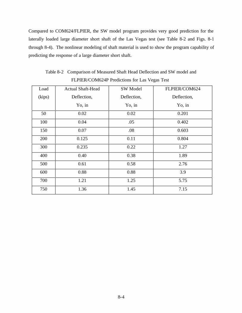
8-4
Compared to COM624/FLPIER, the SW model program provides very good prediction for the
laterally loaded large diameter short shaft of the Las Vegas test (see Table 8-2 and Figs. 8-1
through 8-4). The nonlinear modeling of shaft material is used to show the program capability of
predicting the response of a large diameter short shaft.
Table 8-2 Comparison of Measured Shaft Head Deflection and SW model and
FLPIER/COM624P Predictions for Las Vegas Test
Load
(kips)
Actual Shaft-Head
Deflection,
Yo, in
SW Model
Deflection,
Yo, in
FLPIER/COM624
Deflection,
Yo, in
50 0.02 0.02 0.201
100 0.04 .05 0.402
150 0.07 .08 0.603
200 0.125 0.11 0.804
300 0.235 0.22 1.27
400 0.40 0.38 1.89
500 0.61 0.58 2.76
600 0.88 0.88 3.9
700 1.21 1.25 5.75
750 1.36 1.45 7.15

8-5
8.3 SOUTHERN CALIFORNIA FIELD TEST (SHORT SHAFT)
A number of cast-in-place drilled piers were constructed and tested in Southern California and
reported by Bhushan et al. (1978). The piers were constructed at five different sites. One of
these piers is an ideal short shaft with which to compare the predictive capability and reliability
of computer programs such as LPILE/COM624P/FLPIER and SW model. Regardless of the
predicted results, it should be mentioned again that the p-y curves employed in the programs
LPILE, COM624P or FLPIER were established based on long small diameter piles that are not
representative of large diameter shafts.
In short shaft case reported here, the pier tested was 4 feet in diameter and 16 feet in length. The
pier was constructed in stiff clay with undrained shear strength (Su) of 5500 psf and ε50 of 0.94%
(Table 8-3). This data was reported by Bhushan et al. (1978) and used with COM624 by Reese
(1983) [the developer of the program COM624 and LPILE]. Reese (1983) reported the results
provided by the program COM624 and presented in Fig. 8-5 and Table 8-4. Compared to the
measured data, COM624 provides very soft response. The results assessed using the SW model
program are in good agreement with the field data. Figures 8-6 through 8-8 show the lateral
response of the tested shaft using the SW model technique.
Table 8-3 - Soil Data for Southern California Test
Soil Layer Soil Type Thickness (ft) γ (pcf) φ (deg.) Su (psf) ε50**
Layer 1 Clay 22 130 34 5500 0.0095
Table 8-4 Comparison of Measured Shaft Head Deflection and SW model and COM624P Predictions for Southern California Test
Load
(kips)
Actual shaft-head deflection,
Yo, in
SW model Deflection,
Yo, in
COM624 Deflection,
Yo, in
50 0.1 0.094 0.20
100 0.25 0.2275 0.35
200 0.67 0.59 1.50
300 1.10 1.00 4.40
400 1.85 1.55 15.0

8-6
8.4 TREASURE ISLAND FULL-SCALE LOAD TEST
ON PILE IN LIQUEFIED SOIL
A series of full-scale field tests in liquefied soil was performed at Treasure Island in San
Francisco Bay (Ashford and Rollins 1999). The soil properties employed in the SWM analysis
for the test site based on the reported data (Weaver et al. 2001) are described in Table 8-5. Soil
and pile properties can be also seen in Fig. 8-9. In this analysis, the sand is assumed to contain
5% fines. The soil was liquefied by carrying out controlled blasts at that site without densifying
the soil in the test area. Drained and undrained lateral loading tests were performed on a long
isolated pipe pile filled with concrete (CISS) of 0.61 m diameter. The tested pile exhibited free-
head conditions and was laterally loaded 1.0 m above ground surface. The test pile had bending
stiffness EI = 448320 kN-m2.
The observed and SW model predicted drained response of the pile compares favorably as seen
in Fig. 8-10. Procedures followed in the Treasure Island test (liquefying the soil around the pile
and then loading the pile laterally) subsequent to the static drained test are similar to those
employed with the SW model analysis. The assessed undrained post-liquefaction behavior of the
tested pile is based on the procedures presented herein, and includes the effect of free-field and
near-field excess pore pressure (uxs,ff + uxs,nf). The pile head response shown in Fig. 8-10 is
based on a peak ground acceleration (amax) of 0.11g, and an earthquake magnitude (M) of 6.5.
The piles were cyclically loaded after the first blast at the site. The observed (field) undrained
points (Ashford and Rollins 1999), which are shown in Fig. 8-10, represent the peaks of the
cyclic undrained response of these piles. It should be mentioned that the good agreement
between the measured and predicted undrained response is based on an assumed maximum
ground acceleration, amax, of 0.11g. This value of amax generates high excess porewater pressures
(uxs, ff) in most of the sand layers. It should be noted that the value of amax employed in the
analysis causes an excess porewater pressure ratio (ru) equal to 0.95 in most of the sand and the
best match with the measured free-field excess porewater pressure pattern induced in the field
(Ashford and Rollins 1999).

8-7
Table 8-5. Soil Properties Employed in the SWM Analysis for the Treasure Island Test
Soil Layer
Thick. (m)
Soil Type Unit Weight,
γ (kN/m3)
(N1)60 ö
(degree)
å50
%
Su
KN/m2
0.5 Brown, loose sand (SP) 18.0 16 33 0.45
4.0 Brown, loose sand (SP) 8.0 11 31 0.6
3.7 Gray clay (CL) 7.0 4 1.5 20
4.5 Gray, loose sand (SP) 7.0 5 28 1.0
5.5 Gray clay (CL) 7.0 4 1.5 20
The p-y curve comparisons in Fig. 8-11 show the capability of the SW model for predicting the
p-y curves of a pile/shaft in fully or partially liquefied soils. The back-calculated (measured) p-y
curves at different depths for the 0.61-m cast-in steel-shell (CISS) pile are from Weaver et al.
(2001). Other techniques, such as the traditional p-y curve approach with a reduction multiplier,
do not show the concave-upward pattern of the back-calculated p-y curves.
It was obvious from the uxs, ff distribution measured along the depth of the pile right after the
blast that the upper 4.6 m was almost fully liquefied. The back-calculated (field) p-y curves
shown in Fig. 8-11 were assessed after a few cycles of loading. As a result, the porewater
pressure in the upper 4.5 m of soil reached 1.0. By increasing the peak ground acceleration
(amax) used in the SW model analysis from 0.11g to 0.15g, the whole soil profile completely
liquefies and the pile head response (load-deflection curve) follows the concave-up shape
(increasing slope) as seen in Fig. 8-12.

8-8
8.5 COOPER RIVER BRIDGE TEST AT THE MOUNT PLEASANT SITE,
SOUTH CAROLINA SITECyclic lateral load tests were performed on two large diameter long shafts at the Mount Pleasant
site. Shaft MP-1 (Cast-in-Steel-Shell, CISS, bending stiffness (EI) = 2 x 10⁸ kip-ft2) was 8.33 ft
in diameter while the shaft MP-2 (Cast-in-Drilled Hole, CIDH, EI = 1.38 x 10⁸ kip-ft2) was 8.5 ft
in diameter, each with a one-inch thick steel shell. The lateral load in both cases was applied at a
point 43-inches above the ground surface. The Mount Pleasant site soil profile consists of 40 ft
of loose to medium dense, clean or silty or clayey sands overlaying a thick layer of the Cooper
Marl (S & ME 2000). Table 8-6 summarizes the basic soil properties of the soil profile at the
Mount Pleasant site used in the SW model analysis. Lateral static load tests were carried out on
as-is conditions, and liquefied conditions induced by controlled blasting (Figs. 8-13 and 14) (S &
ME). The blast successfully generated high porewater pressure (ru =1) within most of the upper
38 ft as indicated by the piezometer data.
LPILE analyses for the load test for the project were carried out using (1) the traditional p-y
curve for the 38 feet thick overburden consisting of sandy deposits of ϕ = 35o and γ = 60 pcf and
(2) back calculated p-y curves for the Cooper Marl from O-cell tests as no traditional p-y curves
representative of the Cooper Marl conditions were available. The LPILE results for pre- and
post-liquefaction conditions based on the back-calculated p-y curve from the O-cell tests are
shown in Figs. 8-13 and 14. In contrast, SW model predicted p-y curves for the Cooper Marl
showed good agreement with the back-calculated p-y curve from the O-cell tests. The SW
model results shown in Figs. 8-13 and 14 are based on the p-y curves predicted from the SW
model analysis.

8-9
Table 8-6 Soil Properties Employed in the SW Model Analysis
for the Cooper River Bridge Tests at Mt. PleasantSoil Layer
Thick. (ft)
Soil Type Unit Weight,
γ (pcf)
(N1)60 Ö
(degree)
å50
%
Su
psf
4 Slightly clay
sand (SP-SC)
120 19 34 0.004
9 Sandy clay
(CH)
62 7 30 0.008
16 Very clayey
sand (SC-CL)
62 10 32 0.006
9 Silty sand
(SM)
62 7 30 0.008
80 Cooper Marl 65 20 0.002 4300
LPILE shaft responses for liquefied conditions were computed for various trial values of ru
different from the measured value in order to come up with a reasonable agreement of shaft
response with the field test results. A constant value for ru =0.7 for the upper 38 ft of overburden
used in the LPILE analysis (for shaft MP-1) yields reasonable agreement with the field results
Fig. 8-13). It should be noted that (1) ru measured in the field was very close or equal to one and
(2) use of ru in the LPILE analysis only reduces the buoyant (effective) unit weight of soil
thereby producing a softer shaft responses. ru used with shaft MP-2 in LPILE analysis was not
defined in the report (SM&E 2000).
The SW model analysis for a shaft in liquefied soil depends on several factors: earthquake
magnitude (M); peak ground acceleration (amax); and the soil properties to determine the values
of ru and the additional excess porewater pressure resulting from the superstructure lateral
loading. An earthquake magnitude of 6.5 and amax of 0.1g and 0.3g were used in the SW model
analysis to obtain the shaft responses shown in Figs. 8-13 and 14. It should be noted that amax of
0.3g develops complete liquefaction in the upper 38 ft of soil. Despite the diameter and EI of
shaft MP-1, larger than those of shaft MP-2, shaft MP-2 experienced a post-liquefaction lateral
response stiffer than that of shaft MP-1, as observed in the field test (Figs. 8-13 and 14). The use

8-10
of different values of amax in the SWM analysis is to exhibit the varying shaft response.
Knowing the seismic zone (i.e. M and amax) and soil and shaft properties at a particular site, the
designer will be able to assess the lateral response of a shaft/pile in liquefiable soils using the
SW model computer program. No attempt was made by SM&E 2000 to back calculate the p-y
curves.

8-11
8.6 UNIVERSITY OF CALIFORNIA, LOS ANGELES (UCLA) FULL-SCALE
LOAD TEST ON LARGE DIAMETER SHAFT
A full-scale load test funded by Caltrans on a cast-in-drilled-hole (CIDH) shaft/column was
conducted by UCLA (Janoyan et al. 2001). The 88-ft long shaft/column tested was 6.0 ft in
diameter for the 40 ft above ground and 6.5 ft in diameter for the 48 ft below ground surface.
The configuration of the tested shaft and its material (concrete/steel) properties are shown in Fig.
8-15. The testing was performed at a site with deep alluvial soils consisting of silty clay and
silty, clayey sand. The soil properties employed in the SW model analysis are reported in Table.
8-7. The shaft/column tested was pushed laterally up to failure (the formation of a plastic hinge).
It should be noted that the field results indicate that the shaft responded as an intermediate shaft
which is consistent with the SW model program description.
Figure 8-16 provides a comparison between the experimental and computed moment curvature
response for the 6-ft-diameter shaft cross section. Compared to the results of the X-Section
program (used by Caltrans), the moment-curvature relationship assessed using the SW model
program shows better agreement with the experimental results.
Table 8-7 - Soil Data for the UCLA Test
Soil
layer
Soil type Thickness
(ft)
γ (pcf) Su (psf) ε50
Layer 1 Stiff Clay 6 130 4000 0.003
Layer 2 Stiff Clay 18 130 2500 0.005
Layer 3 Stiff Clay 40 130 3000 0.004
Figure 8-17 shows a comparison between the measured shaft response and the computed one
using LPILE, SWM6.0 and the current shaft program. To obtain good match with field data, a
sand soil profile was used with LPILE (as reported by Caltrans). The data obtained using LPILE
based on the original soil profile shown in Table 8-7 and given in the UCLA report did not
provide good agreement with the measured data. As seen in Fig. 8-16, the same column/shaft

8-12
was previously analyzed using the older SW model program (SWM6.0) for a long piles/shaft that
does not account for the vertical side shear resistance and shaft classification.

8-13
8.7 FULL-SCALE LOAD TEST ON A BORED PILE IN LAYERED
SAND AND CLAY SOIL
A bored 1.5-m-diameter reinforced concrete pile was installed to a depth 34 m below ground
surface in the town of Chaiyi in the west central coastal plain of Taiwan (Fig. 8-18 by Brown et
al. 2001). The pile tested with free-head conditions was laterally loaded at 0.5 m above ground.
As reported by Brown et al (2001), relatively poor comparisons with the measured results were
obtained using the traditional p-y curves for sand (Reese et al. 1974) and clay (Matlock 1970)
with the program FLPIER (McVay et al. 1996). The traditional p-y curves were modified to a
very large extent in the upper 12 m (see the modified p-y curves by Brown et al. 2001 in Fig. 8-
19) in order to obtain good agreement with the measured data for the isolated pile.
Using the original soil properties given by Brown et al. (2001) shown in Fig. 8-18, the SW model
provides an assessed response in good agreement with the measured response of the single free
head pile (Fig. 8-20). A nonlinear model for pile material behavior (reinforced concrete)
incorporated in the SW model analysis is employed in this analysis. It should be noted that none
of the given (original) soil and pile properties was modified for the SW model analysis.
As presented by Brown et al. (2001) FLPIER (McVay et al. 1996) provides excellent agreement
with the measured response by using deduced (adjusted) (site specific) modified p-y curves
shown in Fig. 8-19. The nonlinear modeling of pile material played an important role in the
results obtained by FLPIER and the SW model analyses. Significant recommendations and
comments were made by Brown et al. (2001) relative to a p-multiplier to be used with the
traditional p-y curves.
8.8 SUMMARY
This chapter has demonstrated via comparison with field test results, the capability of the SW
model shaft analysis relative to various applications. The SW model analyses were undertaken
using the unmodified soil and pile properties reported in the literature. Comparable
LPILE/COM24/FLPIER assessments using the traditional p-y curves required moderate to
significant modifications of such data in order to obtain reasonable agreement with overall field
test results. Even so, traditional p-y curves for liquefied sand do not show the concave-upward

8-14
shape that is predicted by the SW model analysis and noted back-calculated curves from the
Treasure Island tests.

8-15
Fig. 8-1 Measured and Computed Shaft Response of the Las Vegas Test
0 2 4 6 8Shaft-Head Lateral Deflection, Yo, in.
0
200
400
600
800
1000
Sha
ft-H
ead
Late
ral L
oad,
Po,
Kip
s
MeasuredS W ModelFLPIER /CO M624P
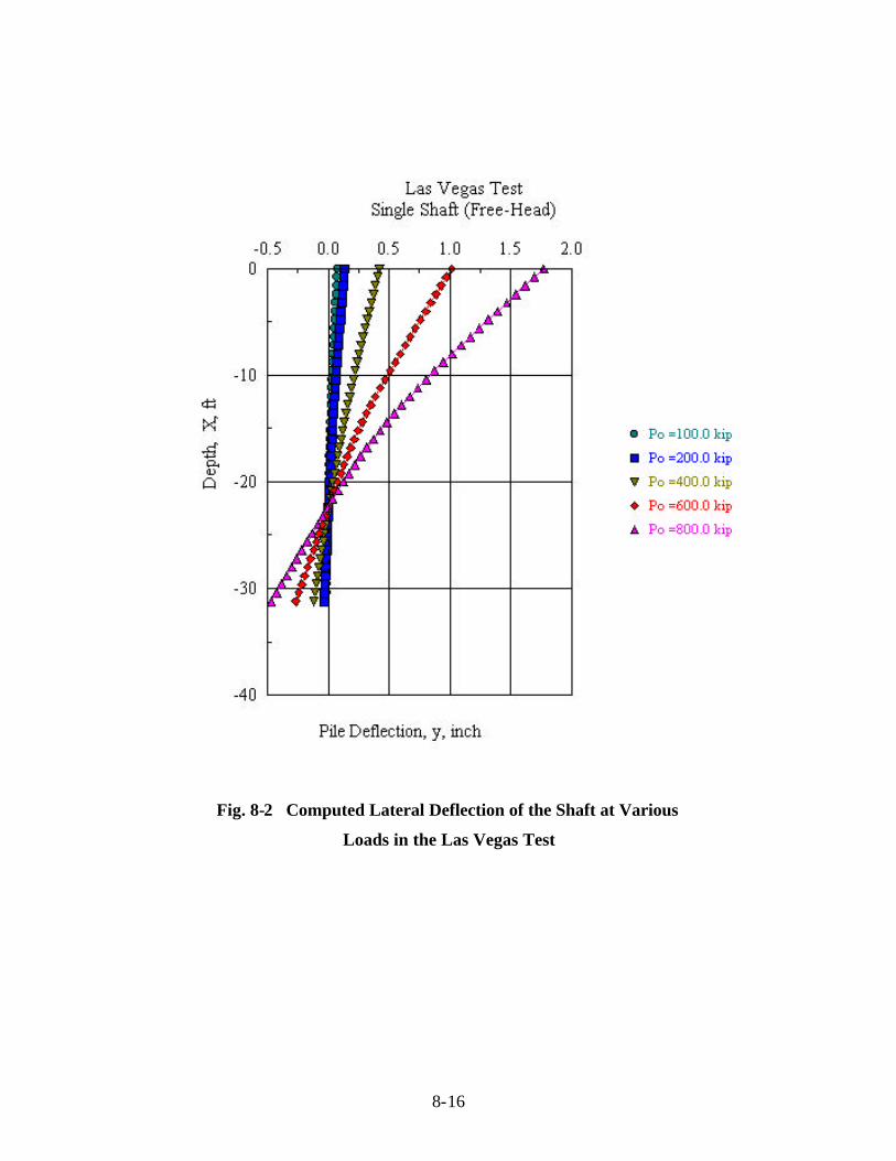
8-16
Fig. 8-2 Computed Lateral Deflection of the Shaft at Various
Loads in the Las Vegas Test

8-17
Fig. 8-3 Computed Bending Moment Distribution in the Shaft in the Las Vegas Test
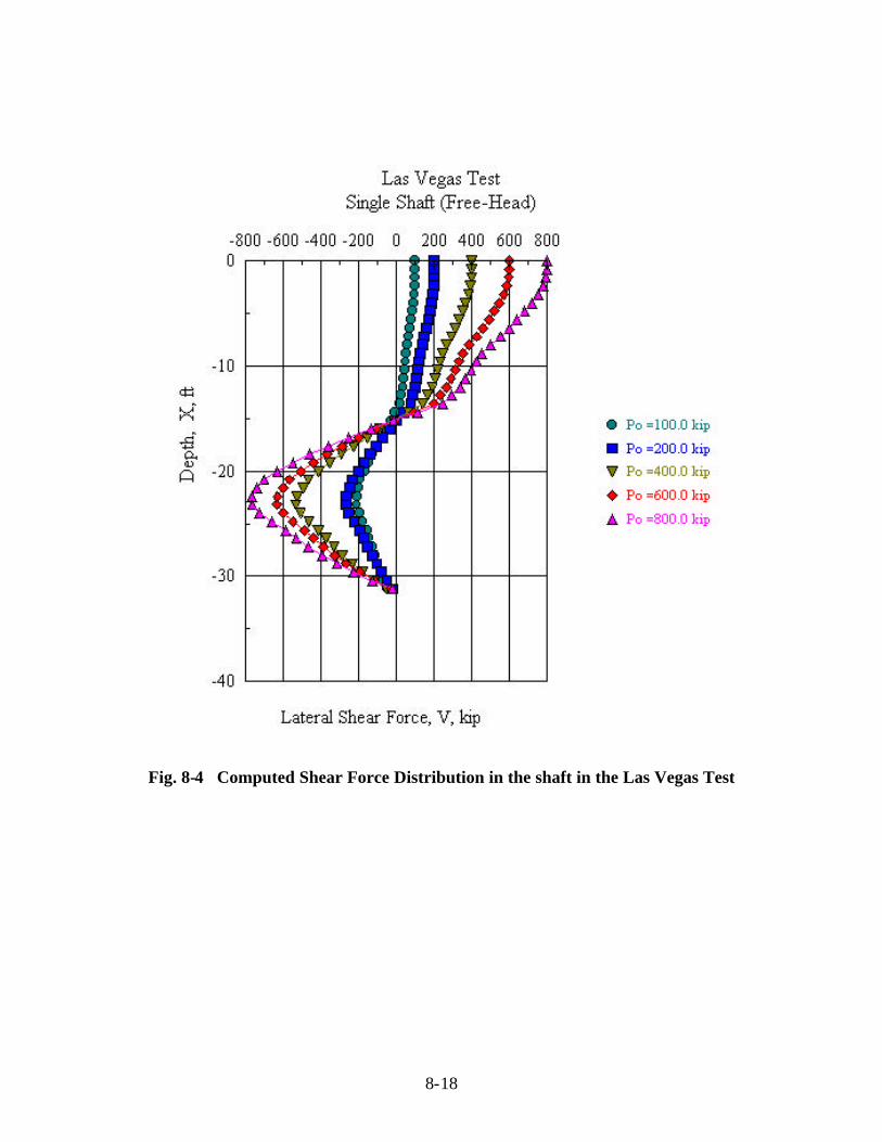
8-18
Fig. 8-4 Computed Shear Force Distribution in the shaft in the Las Vegas Test

8-19
Fig. 8-5 Measured and Predicted Shaft Response of the Southern California Test (Pier 1)
0 1 2 3 4 5Shaft-Head Lateral Deflection, Yo, in.
0
100
200
300
400
Sha
ft-H
ead
Late
ral L
oad,
Po,
Kip
s
MeasuredS-ShaftFLPIER/COM624P

8-20
Fig. 8-6 Computed Lateral Deflection for at the Southern California Test
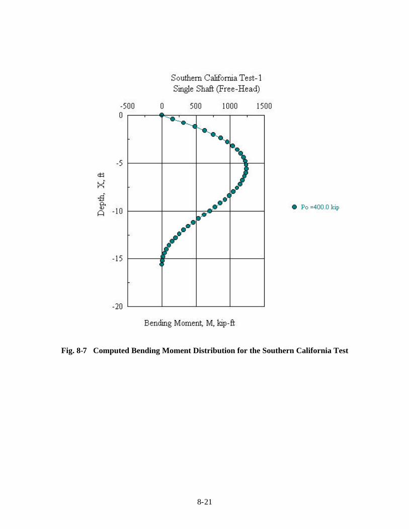
8-21
Fig. 8-7 Computed Bending Moment Distribution for the Southern California Test

8-22
Fig. 8-8 Computed Shear Force in the Shaft in the Southern California Test

8-23
Fig
. 8-9
So
il an
d P
ile P
rope
rtie
s of
the
Tes
t P
erfo
rmed
at
Tre
asur
e Is
land
.
Pile
Hea
d E
leva
tion
( 0.0
0 )
P o
Mo =
0.0
Axi
al L
oad=
0.0
Dia
met
er o
f Pile
Pile Length = 20.0 ft
Th
ickn
ess
of L
ayer
# 2
Th
ickn
ess
of
Lay
er #
3
Wat
er T
able
SAND CLAY
Gro
und
Sur
face
1.0
m
4.0 m 4.0 m
0.61
m
Laye
r th
ickn
ess
= 4.
0 m
Effe
ctiv
e un
it w
eigh
t = 8
.0 k
N/m
3
Effe
ctiv
e fri
ctio
n an
gle
= 31
.0o
e 50
= 0.
006,
(N1)
60 =
11
Laye
r thi
ckne
ss =
3.7
mE
ffect
ive
unit
wei
ght =
7.0
kN
/m3
Effe
ctiv
e fri
ctio
n an
gle
= 24
o or
0.0
(def
ault)
(Su) T
op =
20 k
N/m
2, (
Su) B
otto
m =
20 k
N/m
2
e50
=0.
015
CLAY SAND
4.5 m 7.5 m
0.5
m
Thi
ckn
ess
of
Lay
er
# 4
Laye
r thi
ckne
ss =
5.0
mE
ffect
ive
unit
wei
ght =
7.0
kN/m
3
Effe
ctiv
e fri
ctio
n an
gle
=28.
0o
e 50
= 0.
01, (
N1) 60
= 9
Laye
r thi
ckne
ss =
5.5
mEf
fect
ive
unit
wei
ght =
7.0
kN
/m3
Effe
ctiv
e fri
ctio
n an
gle
= 24
o o
r 0.0
(de
faul
t)(S
u)To
p =20
kN
/m2 ,
(Su) B
otto
m =
20 k
N/m
2
e50
=0.
015
Th
ickn
ess
of L
ayer
# 5
Th
ickn
ess
of L
ayer
# 1
Laye
r th
ickn
ess
=0.5
mE
ffect
ive
unit
wei
ght =
18.
0 kN
/m3
Effe
ctiv
e fri
ctio
n an
gle
=33.
0o
e 50
= 0.
0045
, (N
1)60
= 1
6
% o
f fin
es=
5%
% o
f fin
es=
10%
T-Sh
ell
Pea
k G
roun
d A
ccel
erat
ion
(am
ax) =
0.1
gM
agni
tude
of E
arth
quak
e =
6.5
No
late
ral s
prea
ding
Free
- and
Nea
r-fie
ld e
xces
s po
rew
ater
pre
ssur
e ef
fect
Ass
ume
sand
gra
ins
Sub
angu
lar
Sh
aft
Sec
tion
Num
bers
of s
haft
segm
ents
=1
Segm
ent l
engt
h =
20 m
Shaf
t dia
met
er =
0.6
1mSt
eel s
hell
thic
knes
s =
9.5
mm
f y o
f the
ste
el s
hell =
420
000
kN/
m2
f c o
f con
cret
e =
3444
4 kN
/m2
f y o
f the
ste
el b
ars
= 42
0000
kN/
m2
Rat
io o
f Ste
el b
ars
(As/A
c)= 2
%R
atio
of T
rans
vers
este
el =
0.3
%
Shaf
t Wid
th
xx
Long
itudi
nal
S
teel

8-24
Fig. 8-10 Post-Liquefaction Pile Head Response of the Treasure Island Test
0 50 100 150 200 250Pile-Head Deflection, Yo, mm
0
100
200
300
400
500Pi
le-H
ead
Loa
d, P
o, k
NCISS, 0.61 mEI = 448320 kN-m2
Drained
Observed
Predicted
Undrained
(u + u )xs, ff xs, nf

8-25
Fig. 8-11. Predicted p-y Curves Using the SWM vs. the ObservedOnes from Treasure Island Test.
0 40 80 120 160Pile Lateral Deflection, y (mm)
0
20
40
60
80
p (k
N/m
)
0 40 80 120Pile Lateral Deflection, y (mm)
0
10
20
30
40
50
p (k
N/m
)
Measured Predicted (SW Model)
p-y Curve at 0.2 m Below Ground
Measured Predicted (SW Model)
p-y Curve at 1.5 m Below Ground
0 40 80 120Pile Lateral Deflection, y (mm)
0
10
20
30
40
50
p (k
N/m
)
0 20 40 60 80 100Pile Lateral Deflection, y (mm)
0
10
20
30
40
50
p (k
N/m
)
Measured Predicted (SW Model)
p-y Curve at 2.3 m Below Ground
Measured Predicted (SW Model)
p-y Curve at 3.0 m Below Ground

8-26
Fig. 8-12. Effect of Loading Cycles on Pile Head Response afterLiquefying the Upper Soil Layers (0.61 m Diameter)
0 40 80 120 160 2000
40
80
120
160
200
Pile-Hea
d Load
, Po, kN
0
100
200
300
400
500P
ile-H
ead
Loa
d, P
o, k
N
SW Model in 1st loading cycle
SW Model after few loading cycles

8-27
Fig. 8-13. Lateral Response of Shaft MP-1 at Mount Pleasure Test Site
(Cooper River Bridge)
Fig. 8-14 Lateral Response of Shaft MP-2 at Mount Pleasure Test Site
(Cooper River Bridge)
0 1 2 3 4 5Lateral Shaft-Head Displacement, Yo, in.
0
400
800
1200La
tera
l Loa
d, P
o, k
ips
MeasuredLPILE (Input p-y curve from O-Cell )SWM
Static LoadPost-liquefaction amax = 0.1g
amax = 0.3g
ru = 0.7
0 1 2 3 4 5Lateral Shaft-Head Displacement, Yo, in.
0
400
800
1200
Late
ral L
oad,
Po,
kip
s
MeasuredLPILE (Input p-y curve from O-Cell )SW M
Static LoadPost-liquefaction
amax = 0.1g
amax = 0.3g
ru = not defined

8-28
Fig
. 8-1
5 S
oil a
nd S
haft
Pro
pert
ies
of t
he C
olum
n/Sh
aft
Tes
t P
erfo
rmed
by
the
UC
LA
Sha
ft W
idth
Rei
nfor
ced
Con
cret
e D
rille
d S
haft
xx
Long
itudi
nal
S
teel
Sha
ft S
ectio
n# 1
Segm
ent l
engt
h =
40 ft
Shaf
t dia
met
er =
6.0
ftf c
of c
oncr
ete
= 61
00 p
sif y
of t
he s
teel
bar
s =
71 K
siR
atio
of S
teel
bar
s (A
s/Ac)=
2%
Rat
io o
f Tra
nsve
rses
teel
(A'
s/Ac)=
0.5
%
Sha
ft S
ectio
n# 2
Seg
men
t len
gth
= 48
ftS
haft
diam
eter
= 6
.5 ft
f c o
f con
cret
e =
6100
psi
f y o
f the
ste
el b
ars
= 71
Ksi
Rat
io o
f Ste
el b
ars
(As/A
c)=
1.8%
Rat
io o
f Tra
nsve
rses
teel
(A
' s/A
c)= 0
.5%

8-29
Fig. 8-16 Moment-Curvature Relationship of the 6-ft-Diamter Cross-Section
0
50000
100000
150000
200000
250000
300000
350000
-5 0 5 10 15 20
Lateral Deflection, inches
Lo
ad, l
bs
ExperimentUsing 2-ft Fill & 60% of EcUsing 3-ft Hard Fill & Nonlinear EI from LPILESWM6.0Shaft
Fig. 8-17 Comparison Between Measured and Computed Lateral Deflection of the shaft tested at UCLA
0
2000
4000
6000
8000
10000
12000
14000
16000
18000
0.0000 0.0001 0.0002 0.0003 0.0004 0.0005 0.0006 0.0007 0.0008
Curvature φ φ (1/in)
Mo
men
t (ki
p-f
t)
Experimental X_Sectionswm

8-30
Fig. 8-18 Original Soil Profile and Pile Tested at the Chaiyi Test, Taiwan (Brown et al. 2001)
-0.5 m 0.0 m
3.0 m
8.0 m
12.0 m
17.0 m
25.0 m
32.0 m
n= 35o
(= 19 kN/m3
n= 35o
(= 9.2 kN/m3
n= 34o
(= 9.4 kN/m3
n= 34o
(= 9.2 kN/m3
Su=121.3 kN/m2
(= 9.2 kN/m3
g50 = 0.005
Su=115 kN/m2
(= 9.2 kN/m3
g50 = 0.005
Su=60 kN/m2
(= 9.2 kN/m3
g50 = 0.007
Sand
Sand
Sand
Sand
Clay
Clay
Clay
Free head pile

8-31
Fig. 8-19 Traditional p-y Curves Modified to Obtain Good Match with Field Data (Chaiyi Test, Brown et al. 2001)

8-32
Fig. 8-20 Measured Vs. Computed Pile-Head Deflections and the Effect of Vertical Side Shear
0 40 80 120 160 200Pile Head Deflection, Yo, mm
0
1000
2000
3000
4000
Pile
Hea
d Lo
ad, P
o, kN
Measured (Brown et al. 2001)Predicted (SW Model)No V. Side ShearWith V. Side Shear
1.5-m Bored Pile (B1)Free-head

REFERENCES:
Ashford, S. A., and Rollins, K. (1999). “Full-scale behavior of laterally loaded deepfoundations in liquefied sands.” Report No. TR-99/03, Struct. Engg Dept., University ofCalif., San Diego
Ashour, M. and Norris, G. (2000). “Modeling Lateral Soil-Pile Response Based on Soil-Pile Interaction.” Journal of Geotechnical and Geoenvironmental Engineering, ASCE,Vol. 126, No. 5, pp. 420-428.
Ashour, M. and Norris, G. 1999. “Liquefaction and undrained response evaluation ofsands from drained formulation.@ J. of Geotech. Engg, ASCE, Vol. 125, No. 8, pp. 649-658.
Ashour, M., Norris, G. M., Bowman, S., Beeston, H, Billing, P. and Shamsabadi, A.(2001). “Modeling Pile Lateral Response in Weathered Rock..” Proceeding 36st
Engineering Geology and Geotechnical Engineering Symposium, Las Vegas, Nevada,March 26-29.
Ashour, M., Norris, G., and Pilling, P. (1998). “Lateral Loading of a Pile in Layered SoilUsing the Strain Wedge Model.” Journal of Geotechnical and GeoenvironmentalEngineering, ASCE, Vol. 124, No. 4, pp. 303-315.
Ashour, M., Pilling, P., Norris, G., and Perez, H.. (1996). “Development of StrainWedge Model Program for Pile Group Interference and Pile Cap Contribution Effects.”CCEER, Report No. 96-4, Civil Engrg Dept., University of Nevada, Reno.
Ashour, M. and Norris, G. M. (2001). “Pile Group Program for Full Material Modelingand Progressive Failure.” Report No. CCEER-01-02, Civil Engineering Dept. Universityof Nevada, Reno, Contract No. 59A0160, Submitted to State of California Department oftransportation (CalTrans)
Ashour, M. and Norris, G. M. (2000). “Undrained Lateral Pile and Pile Group Responsein Saturated Sand.” Report No. CCEER-00-01, Civil Engineering Dept. University ofNevada, Reno, Federal Study No. F98SD01, Submitted to State of California Departmentof Transportation (CalTrans)
Ashour, M. and Norris, G. M. (1999). “Refinement of the Strain wedge ModelProgram.” Report No. CCEER-99-8, Civil Engineering Dept. University of Nevada,Reno, Federal Study No. F99STD21, Submitted to State of California Department oftransportation (CalTrans)
Norris, G. M., and Ashour, M. “Liquefaction and Undrained Response Evaluation ofSands From Drained Formulation.” Report No. CCEER-98-2, Civil Engineering Dept.,University of Nevada, Reno, May 1998, Project No. DACW39-94-M-5638 (Army Corpsof Engineers)

Bhushan, K., Haley, S. C., and Fong, P. T. (1979). “Lateral Load Tests on Drilled Piersin Stiff Clays.” Journal of Geotechnical Engineering, ASCE, Vol. 105, No. GT8, pp. 969-985.
Bolton, M. D. (1986). ‘The Strength and Dilatancy of Sand.” Geotechnique, 36 (1), pp65-78.
Briaud, J. L., Smith, T., and Mayer, B. (1984). “Laterally Loaded Piles and thePressuremeter: Comparison of Existing Methods.” Laterally Loaded Deep Foundations,ASTM, STP 835, pp. 97-111.
Butterfield, R. and Banerjee, P. K. (1971). “The Elastic Analysis of Compressible Pilesand Pile Groups.” Geotechnique, London, England, Vol. 21, pp. 43-60.
Coyle, H. M. and Reese, L. C. (1966). “Load Transfer for Axially Loaded Piles in Clay.”Journal of Soil Mechanics and Foundations Division, ASCE, Vol. 92, NO. SM2.
Design Manual 7.1 (DM 7.1) (1986). “Soil Mechanics.” Naval Facilities Engg.Command, 200 Stovall str., Alexandria, Virginia 22332-2300.
Design Manual 7.2 (DM 7.2) (1986). “Foundations and Earth Structures.” NavalFacilities Engg. Command, 200 Stovall str., Alexandria, Virginia 22332-2300.
Elfass, S. (2001). “A New Approach For Estimating The Axial Capacity of Driven PilesIn Sand Up To True Soil Failure,” Ph.D. Thesis, University of Nevada, Reno.
Gowda, P. (1991). “Laterally Loaded Pile Analysis for Layered Soil Based on the StrainWedge Model.” M. S. Thesis, University of Nevada, Reno.
Grosch, J. J. and Reese, L. C. (1980). “Field Tests of Small-Scale Pile Segments in aSoft Clay Deposit under Repeated Loading.” Proceedings, 12th offshore TechnologyConference, Houston, TX, Vol. 4, pp. 143-151
Holmquist, D. V. and Matlock, H. (1976). “Resistance-Displacements Relationships forAxially Loaded Piles in Soft Clay.” Proceedings, 8th offshore Technology Conference,Houston, TX, Vol. 1, pp. 553-569
Janoyan, K., Stewart, J. P. and Wallace, J. W. (2001). “Preliminary Test Results for FullScale Drilled Shaft Under Cyclic Lateral Loading.” Report to Caltrans No. 59A0183,Civil Eng. Dept., UC Los Angeles.
Kraft, L. M., Richard, P. R. And Kagawa, T. (1981). “Theoretical t-z Curves.” J. ofGeotech. Engg. Division,. ASCE, Vol. 107, GT11, pp. 1543-1561.

Mander, J. B., Briestley, M. J. N., and Park, R. (1988). “Theoretical Stress-Strain Modelfor Confined Concrete.” Journal of Structural Engineering, ASCE, Vol. 114, No. 8, pp.1804-1826.
Matlock, H. (1970). “Correlations for Design of Laterally Loaded Piles in Soft Clay.”The 2nd Annual Offshore Technology Conference, Houston, Texas, OTC 1204, pp. 577-607.
Matlock, H. and Reese, L. C. (1961). “Generalized Solution for Laterally Loaded Piles.”Journal of Soil Mechanics and Foundations Division, ASCE, Vol. 86, No. SM5, pp. 673-694.
Meyerhof, G. G. (1956). “Penetration Tests and Bearing Capacity of CohesionlessSoils.” ASCE J., Foundation Division 89, No. SM1, Paper 866, pp. 5-10.
NAVFAC (1982). “Foundations and Earth Retaining Structures Design manual.” Dept. ofnavy, DM 7.2, Alexandria, VA.
Nguyen, T. Q. 2002. “Sand Behavior from Anisotropic and Isotropic Static and DynamicTriaxial Tests.” Ph.D. Dissertation, Civil Engg. Dept., Univ. of Nevada, Reno, January.
Norris, G. M. (1977). “The Drained Shear Strength of Uniform Quartz Sand as Related toParticle Size and Natural Variation in Particle Shape and Surface Roughness.” Ph.D.Thesis, University of California , Berkeley, 523 pp.
Norris, G. M. (1986). “Evaluation of the Nonlinear Stabilized Rotational Stiffness of PileGroups.” Proceedings of the 37th Annual Highway Geology Symposium, Montana Dept.of Highways, Helena, Montana.
Norris, G. M. (1986). “Theoretically Based BEF Laterally Loaded Pile Analysis.” ThirdInternational Conference on Numerical Methods in Offshore Piling, Nantes, France, pp.361-386.
Norris, G., Siddharthan, R., Zafir, Z., and Madhu, R. 1997. “Liquefaction and residualstrength of sands from drained triaxial tests.@ J. of Geotech. Engg, ASCE, Vol. 123, No.3, pp. 220-228.
Norris, G., Zafir, Z., and Siddharthan, R. 1998. “An effective stress understanding ofliquefaction behavior.” Journal of Environmental & Engineering Geoscience, Vol. 4, No.1 pp. 93-101.
Paulay, T., and Priestley, M. J. N. (1992). “Seismic Design of Reinforced Concrete andMasonry.” Johen Wiley and Sons, New York, N.Y., pp. 95-157.
Poulos, H. G. and Davis, E. H. (1968). “The Settlement Behavior of Single, Axially

Loaded Incompressible Piles and Piers.” Geotechnique, London, England, Vol. 18, pp.351-371.
Randolph, M. F. and Worth, C. P. (1978). “Analysis of Deformation of VerticallyLoaded Piles.” J. of Geotech. Engg. Division,. ASCE, Vol. 104, GT12, pp. 1465-1488.
Reese, L. C. (1958). “Discussion of Soil Modulus for Laterally Loaded Piles.” byBramlette McClelland and John A. Focht, Jr., Transactions, ASCE, Vol. 123, pp. 1071.
Reese, L. C. (1977). “Laterally Loaded Piles: Program Documentation.” Journal ofGeotechnical Engineering, ASCE, Vol. 103, No. GT4, pp. 287-305.
Reese, L. C. (1983). “Behavior of Piles and Pile Groups Under Lateral Load.” Report tothe U.S. Department of Transportation, Federal Highway Administration, Office ofResearch, Development, and Technology, Washington, D.C.
Reese, L. C. (1984). “Handbook on Design of Piles and Drilled Shafts under LateralLoad.” Geotechnical Engineering Center, Bureau of Engineering Research, University ofTexas at Austin., Report No. FHWA-IP-84-11
Reese, L. C. (1987). “Documentation of The Computer Program LPILE1.” Ensoft Inc.,Post Office Box 180348, Texas 78718.
Reese, L. C. and Wang S. T. (1994). “Analysis of piles under lateral loading withnonlinear flexural rigidity.” U.S. FHWA Int. Conf. On Design and Construction of DeepFoundation, FHWA, Washington, D.C.
Richart, E. F. (1975). “Some Effects of dynamic Soil Properties on Soil-StructureInteraction.” J. of Geotech. Engg. Division,. ASCE, Vol. 101, GT12, pp. 1197-1240.
Robinsky, E. I. And Morrison, C. E. (1964). “Sand Displacement and CompactionAround Model Friction Piles.” Canadian Gotech. J., Vol. 1, No. 2, p. 81.
S&ME Inc. (2000). “Cooper River Bridge replacement project, Charleston, SouthCarolina.”Report prepared by S $ ME, Inc., 840 Low Country Blvd, Mt. Pleasant, SC29464.
Schnertmann, J. H. (1970). “Static Cone to Compute Static Settlement Over Sand.”. J. ofGeotech. Engg. Division,. ASCE, Vol. 96, SM3, pp. 1011-1043.
Schnertmann, J. H., Hartman, J. P. And Brown, P. R. (1979). “Improved Strain InfluenceFactor Diagram.” J. of Geotech. Engg. ASCE, Vol. 105, No. GT6, pp. 715-726.
Seed, H. B. 1979. “Considerations in the earthquake-resistance design of earth androckfill dams.” Geotechnique 29, No. 3, pp. 215-263.

Seed, H. B. And Reese, L. C. (1957). “The action of Soft Clay along Friction Piles.”Transactions, ASCE, Vol. 122.
Seed, R. B. and Harder, L. F. 1990. “SPT-based analysis of cyclic pore pressuregeneration and undrained residual strength.@ Vol. 2, BiTech Publishers Ltd, Vancouver,B. C., Canada.
Skempton, A. W. (1951). “The Bearing capacity of Clays.” Proceedings, Bldg, ResearchCongress, Inst. Og Civil Engineering, London, Eng., 1951, Vol. I.
Skempton, A. W. (1954). “The Pore Pressure Coefficients A and B.” Geotechnique, 4,pp. 148.
Terzaghi, K. (1955). “Evaluation of Coefficients of Subgrade Reaction.” Geotechnique,Vol. 5, No. 4, pp. 297-326.
The 2nd Annual Offshore Technology Conference, Houston, Texas, OTC 1204, pp. 577-Thesis, University of California , Berkeley, 523 pp.
Tomlinson, M. J. (1957). ”The Adhesion of Piles Driven in Clay Soils.” Proceedings ofFourth International Conf. on Soil mechanics and Foundation Engrg, Vol. II, London, pp.66-71.
Triaxial Tests.” Ph.D. Dissertation, Civil Engg. Dept., Univ. of Nevada, Reno, January.Vaid, Y. P. And Thomas, J. 1995. “Liquefaction and post-liquefaction of behavior ofsand.” J. of Geotech. Engg, ASCE, Vol. 121, No. 2, pp. 163-173.
Vesic, A. (1961). “Bending of Beams Resting on Isotropic Elastic Solid.” Journal, ASCE,Engineering Mechanics Div., Vol. 87, SM 2, pp. 35-53.
Vesic, A. S. (1970). “Tests on Instrumented Piles, Ogeechee River Site.” Journal of SoilMechanics and Foundations Division, ASCE, Vol. 96, No. SM2, pp. 561-584.
Weaver, T. J., Ashford, S. A. and Rollins, K. M. (2001). “Development of p-y curves fora 0.6-m CISS pile in liquefied sand.” The 6th Caltrans Seismic Research WorkshopProgram, June 12th-13th, Paper No. 5-104
Wu, T. H. (1966). Soil Mechanics, Boston, Allyn and Bacon Inc., pp. 169.
Zafir, Z. and Vanderpool, W. (1998). “Lateral Response of Large Diameter DrilledShafts: I-15/US 95 Load Test Program.” 33rd Engineering Geology and GeotechnicalEngineering Symposium, March 25-27, Reno, Nevada, pp. 161-176.
Hughes, J. M. O., Goldsmith, P. R., and Fendall H.D.W. 1978. “The Behavior of Piles toLateral Loads.” Civil Engg. Dept., Univ. of Auckland, Auckland, New Zealand, ReportNo. 178.

Rowe, P. W. (1956). “The Single Pile Subject to Horizontal Force.” Geotechnique, Vol.6.