analysis of slope stability for waste dumps in a mine - ethesis
TRANSCRIPT
ANALYSIS OF SLOPE STABILITY FOR WASTE DUMPS IN A MINE
A THESIS SUBMITTED IN PARTIAL FULFILLMENT OF THE
REQUIREMENTS FOR THE DEGREE OF
Bachelor of Technology in Mining Engineering
by
GORAKINKAR DAS
Department of Mining Engineering
National Institute of Technology Rourkela-769008
2011
ANALYSIS OF SLOPE STABILITY FOR WASTE DUMPS IN A MINE
A THESIS SUBMITTED IN PARTIAL FULFILLMENT OF THE
REQUIREMENTS FOR THE DEGREE OF
Bachelor of Technology in Mining Engineering
by
GORAKINKAR DAS 107MN034
Under the guidance of
Dr. MANOJ KUMAR MISHRA
Department of Mining Engineering
National Institute of Technology Rourkela-769008
2011

i
NATIONAL INSTITUTE OF TECHNOLOGY
ROURKELA
CERTIFICATE
This is to certify that the thesis entitled, “Analysis of Slope Stability for Waste Dumps in a
Mine” submitted by Mr Gorakinkar Das, Roll No. 107MN034 in partial fulfilment of the
requirement for the award of Bachelor of Technology Degree in Mining Engineering at the
National Institute of Technology, Rourkela (Deemed University) is an authentic work carried out
by him under my supervision and guidance.
To the best of my knowledge, the matter embodied in the thesis has not been submitted to any
University/Institute for the award of any Degree or Diploma.
Date:
Dr. M. K. Mishra
Department Of Mining Engineering
National Institute of Technology
Rourkela – 769008

ii
ACKNOWLEDGEMENT
First and foremost, I express my profound gratitude and indebtedness to Dr. M. K. Mishra,
Professor of Department of Mining Engineering for allowing me to carry on the present topic
“Analysis of Slope Stability for Waste Dumps in a Mine” and later on for his inspiring
guidance, constructive criticism and valuable suggestions throughout this project work. I am very
much thankful to him for his able guidance and pain taking effort in improving my
understanding of this project.
I am thankful to Mr Ajay Behera & his esteemed organization for providing the samples for the
project work.
All the experimental analysis done in this project would not have been possible without the help
of Ms Banita Behera, Research Scholar, Dept. of Mining Engineering. I extend my sincere
thanks to her.
I am also thankful to Dr. S. Chatterjee for guiding me in completing Monte-Carlo Simulations.
An assemblage of this nature could never have been attempted without reference to and
inspiration from the works of others whose details are mentioned in reference section. I
acknowledge my indebtedness to all of them.
At the last, my sincere thanks to all my friends who have patiently extended all sorts of helps for
accomplishing this assignment.
Date: Gorakinkar Das
iii
CONTENTS
Page No
CERTIFICATE i
ACKNOWLEDGEMENT ii
ABSTRACT vi
LIST OF TABLES vii
LIST OF FIGURES ix
1. INTRODUCTION
1.1. Background of the problem 1
1.2. Aim of the Study 2
1.3. Methodology 3
2. LITERATURE REVIEW
2.1. Stability Analysis – General Concepts 4
2.2. Factors affecting slope stability 6
2.3. Sliding Block Analysis 7
2.4. Phreatic Surface 9
2.5. Effect of Tension Cracks 9
2.6. Limit equilibrium analysis 9
2.7. Methods of Slices 10
2.8. Probabilistic Analysis 13
2.9. Slope Stability Analysis System – GALENA 19
3. EXPERIMENTAL TECHNIQUES AND RESULTS
3.1. General Description of the Mine 23
3.2. Field Observations 24
3.3. Sample Collection and Preparation 26
3.4. Experimental Methods 27
3.5. Mohr Coulomb Analyses 33
iv
4. ANALYSIS
4.1. Valuation of Factor of Safety 38
4.2. Monte Carlo Simulation 43
4.3. Calculation of Reliability Index 49
4.4. Proposing the optimum slope Height 53
4.5. Proposed Individual Bench 54
5. CONCLUSION AND RECOMMENDATION
5.1. Conclusion 55
5.2. Recommendation 55
REFERENCES 57
v
ABSTRACT
In the civilized world mining activities are synonymous with the standard of life as well as
the state of any nation. It results in both economic and uneconomic materials being
generated. The Uneconomic materials (Wastes) are stacked at different places known as
waste dumps. The stability of these dumps has been a major concern over the years. The
problem becomes increasingly difficult with the reduced availability of land areas for
dumping. In this project, the slope stability analysis for the waste dump of a local Iron Mine
has been carried out. Samples are collected and tasted in the laboratory to find out different
geo-technical parameters. The Factors of Safety of the various sections are calculated using
Limit Equilibrium Method. Probabilistic analysis (Monte Carlo Simulation) has also been
carried out to evaluate the stability of the existing design data. At the end bench design as
well as corresponding safety factors has been developed based on the analysis.
vi
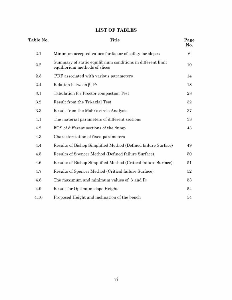
LIST OF TABLES
Table No. Title Page
No.
2.1 Minimum accepted values for factor of safety for slopes 6
2.2 Summary of static equilibrium conditions in different limit
equilibrium methods of slices 10
2.3 PDF associated with various parameters 14
2.4 Relation between , Pf 18
3.1 Tabulation for Proctor compaction Test 28
3.2 Result from the Tri-axial Test 32
3.3 Result from the Mohr‟s circle Analysis 37
4.1 The material parameters of different sections 38
4.2 FOS of different sections of the dump 43
4.3 Characterization of fixed parameters
4.4 Results of Bishop Simplified Method (Defined failure Surface) 49
4.5 Results of Spencer Method (Defined failure Surface) 50
4.6 Results of Bishop Simplified Method (Critical failure Surface). 51
4.7 Results of Spencer Method (Critical failure Surface) 52
4.8 The maximum and minimum values of and Pf. 53
4.9 Result for Optimum slope Height 54
4.10 Proposed Height and inclination of the bench 54
vii
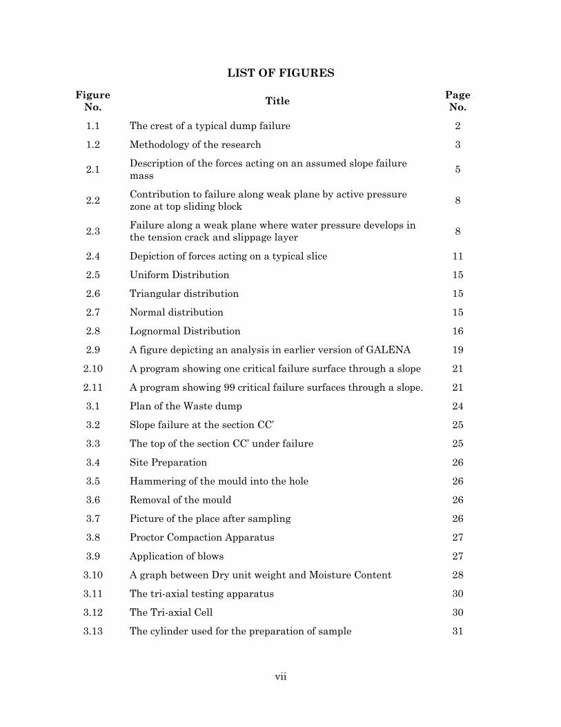
LIST OF FIGURES
Figure
No. Title
Page
No.
1.1 The crest of a typical dump failure 2
1.2 Methodology of the research 3
2.1 Description of the forces acting on an assumed slope failure
mass 5
2.2 Contribution to failure along weak plane by active pressure
zone at top sliding block 8
2.3 Failure along a weak plane where water pressure develops in
the tension crack and slippage layer 8
2.4 Depiction of forces acting on a typical slice 11
2.5 Uniform Distribution 15
2.6 Triangular distribution 15
2.7 Normal distribution 15
2.8 Lognormal Distribution 16
2.9 A figure depicting an analysis in earlier version of GALENA 19
2.10 A program showing one critical failure surface through a slope 21
2.11 A program showing 99 critical failure surfaces through a slope. 21
3.1 Plan of the Waste dump 24
3.2 Slope failure at the section CC‟ 25
3.3 The top of the section CC‟ under failure 25
3.4 Site Preparation 26
3.5 Hammering of the mould into the hole 26
3.6 Removal of the mould 26
3.7 Picture of the place after sampling 26
3.8 Proctor Compaction Apparatus 27
3.9 Application of blows 27
3.10 A graph between Dry unit weight and Moisture Content 28
3.11 The tri-axial testing apparatus 30
3.12 The Tri-axial Cell 30
3.13 The cylinder used for the preparation of sample 31

viii
3.14 Sample of size 3.75mm 31
3.15 Preparation of the sample 31
3.16 Cylindrical sample before Test 32
3.17 Sample after the test 32
3.18 Mohr‟s circle for Sample 1 33
3.19 Mohr‟s circle for Sample 2 34
3.20 Mohr‟s circle for Sample 3 34
3.22 Mohr‟s circle for Sample 5 35
3.23 Mohr‟s circle for Sample 6 35
3.24 Mohr‟s circle for Sample 7 36
3.25 Mohr‟s circle for Sample 8 36
4.1 Design of the section AA‟ 39
4.2 The output of the section AA‟ 39
4.3 Design of the section BB‟ 40
4.4 The output of the section BB‟ 40
4.5 Design of the section CC‟ 41
4.6 The output of the section CC‟ 41
4.7 Design of the section DD‟ 42
4.8 The output of the section DD‟ 42
4.9 Normal Distribution curves for Cohesion and Angle of Friction
(Bench A) 43
4.10 Normal Distribution curve for Cohesion and Angle of Friction
(Bench B) 44
4.11 MCS with 100 iterations 45
4.12 MCS with 500 iterations 45
4.13 MCS with 1000 iterations 45
4.14 MCS with 2000 iterations 46
4.15 MCS with 3000 iterations 46
4.16 MCS with 4000 iterations 46
4.17 MCS with 5000 iterations 47
4.18 MCS with 6000 iterations 47
4.19 MCS with 7000 iterations 47
ix
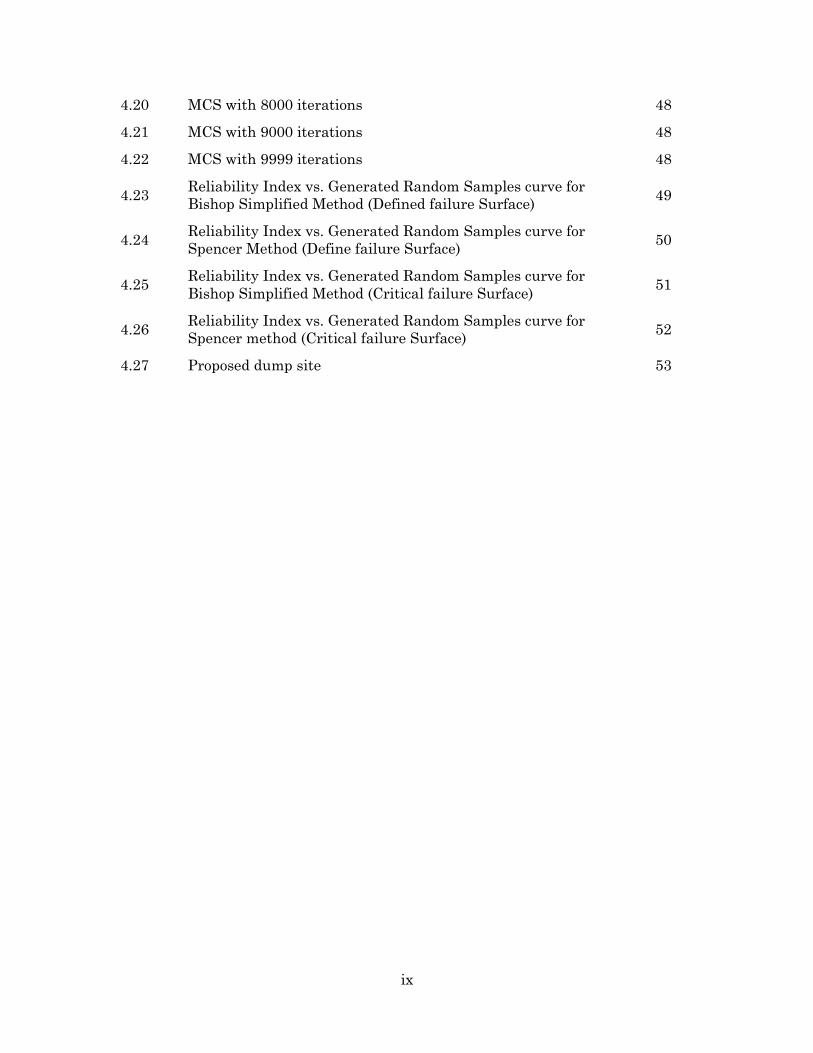
4.20 MCS with 8000 iterations 48
4.21 MCS with 9000 iterations 48
4.22 MCS with 9999 iterations 48
4.23 Reliability Index vs. Generated Random Samples curve for
Bishop Simplified Method (Defined failure Surface) 49
4.24 Reliability Index vs. Generated Random Samples curve for
Spencer Method (Define failure Surface) 50
4.25 Reliability Index vs. Generated Random Samples curve for
Bishop Simplified Method (Critical failure Surface) 51
4.26 Reliability Index vs. Generated Random Samples curve for
Spencer method (Critical failure Surface) 52
4.27 Proposed dump site 53

1 | P a g e
CHAPTER - 1
INTRODUCTION
1.1 Background of the problem
In the modern world mining has become an essential act for the production of economic
minerals. In the production process huge amount of wastes are generated. These waste
materials are stacked in a convenient place for its further use or disposal, or are stored
permanently. They are stored in the form of a slope or embankment. In either of the
purposes the stability of the slope has been a major concern.
The region affected by the slope failure is always not necessarily the slope‟s immediate
area. The stability of sloped land areas, landslide, is a main concern where movements of
existing or planned slopes would have an effect on the safety of people and property or the
usability and value of the area.
Constantly appearing disasters have a great weight on the issue of slope stability. The
disasters and devastation include the natural events (torrential rains), uncased
excavations, road embankments and landfills. The quoted phenomena take place due to
either an incorrect approach to the assessment of their stability, or mistakes made at the
stage of geotechnical investigations, erroneous assumptions made in the phase of carrying
out calculation, or an improper location of machines on the slope surcharge.
One of the causes of the incorrect assessment of slope stability may be inaccurate
determination of the geological structure of the slope in question. As the mine expands over
a period of time, these waste dumps and the issues regarding their stability become
important. To deal with these slope stability issues various approaches have been adopted
and developed over the years. The approaches now have been more of computational rather
than the manual. Various software are available to analyze the slopes that are liable to
failure by the calculating the factor of safety.
Of particular relevance to slope stability analysis are the finite elements and limit
equilibrium methods. However, when using limiting equilibrium methods to analyze slopes,
several numerical inconsistencies and computational difficulties may occur in locating the
critical slip surface (depending on the geology) and hence establishing a factor of safety.
Despite these inherent limitations, due to its simplicity limiting equilibrium continues to be
the most commonly used approach. [N. A. Hammouri et al. 2008]

2 | P a g e
Fig 1.1: The crest of a typical dump failure. (Source: E. Steiakakis et al., 2009)
1.2 Aim of the Study
The objective of this project is to investigate the stability of the slopes by determining the
factor of safety and to propose different safe slopes. This has been achieved by the following
specific objectives.
1.2.1 Specific Objectives:
The primary objective of this project is to evaluate the stability of the slopes constructed
due to dumping of the waste materials (especially the sub-grade materials). It has the
following specific objectives:
Critical review of the available literature to understand the issues involved.
Collection of samples from field or an operating mine.
Analysis of the samples to find out parametric variations (as the cohesion, angle of
friction, density, moisture content, grain sizes, etc.) affecting the stability.
Prediction of safety factor based on the geotechnical data.
Determination of Reliability Index using Monte Carlo Simulation.
Valuation of the safety factors and suggestion of alternate geometry.
3 | P a g e
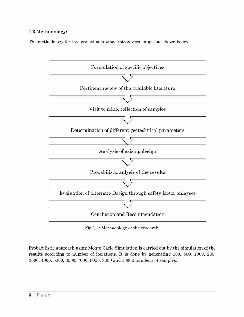
1.3 Methodology:
The methodology for this project is grouped into several stages as shown below.
Fig 1.2: Methodology of the research.
Probabilistic approach using Monte Carlo Simulation is carried out by the simulation of the
results according to number of iterations. It is done by generating 100, 500, 1000, 200,
3000, 4000, 5000, 6000, 7000, 8000, 9000 and 10000 numbers of samples.
Conclusion and Recommendation
Evaluation of alternate Design through safety factor anlayses
Probabilistic anlysis of the results
Analysis of exising design
Determination of different geotechnical parameters
Visit to mine, collection of samples
Pertinent review of the available literature
Formulation of specific objectives
4 | P a g e
CHAPTER - 2
LITERATURE REVIEW
2.1 Stability Analysis – General Concepts (McCarthy & David, 2007)
The slope stability analyses are generally performed to appraise the safe and economic
design of human-made or natural slopes (e.g. embankments, open-pit mining, excavations,
landfills etc.) and the equilibrium conditions. The term „slope stability‟ may be defined as
the ratio of the resistance of inclined surface to failure by sliding or collapsing. The main
objectives of slope stability analysis are ascertaining endangered areas, investigating
potential failure mechanisms, finding of the slope sensitivity to different triggering
mechanisms, designing of optimal slopes with regard to safety, reliability and economics,
designing possible remedial measures, e.g. barriers and stabilization.
Where the stability of a sloped earth mass is to be studied for the possibility of failure by
sliding along a circular slip surface, the principles of engineering statics can be applied to
determine if a stable or unstable condition exists. When the total sliding mass is assumed
to be cylindrical or spoon-shaped, a unit width extending along the face of the slope is taken
for analysis, and the slip surface of the slope cross section is the segment of a circle. Forces
that would affect the equilibrium of the assumed failure mass are determined, and
rotational moments of these forces with respect to a point representing the center of the slip
circle arc (the point is actually an axis in space parallel to the face of the slope) are
computed. With this procedure, the weight of soil in the sliding mass being considered as
well as external loading on the face and top of the slope contribute to the moments acting to
cause movement. Resistance to sliding is provided by the shear strength of the soil on the
assumed slip surface.
A computational method used to indicate if failure (sliding) occurs is to compare moments
that would resist movement to those that tend to cause movement. The maximum shear
strength possessed by the soil is used in the calculation of the resisting moment. Failure is
indicated when moments causing motion exceed those resisting motion. The factor of safety
against sliding or movement is expresses as:
F
5 | P a g e
d2
O
Radius, r
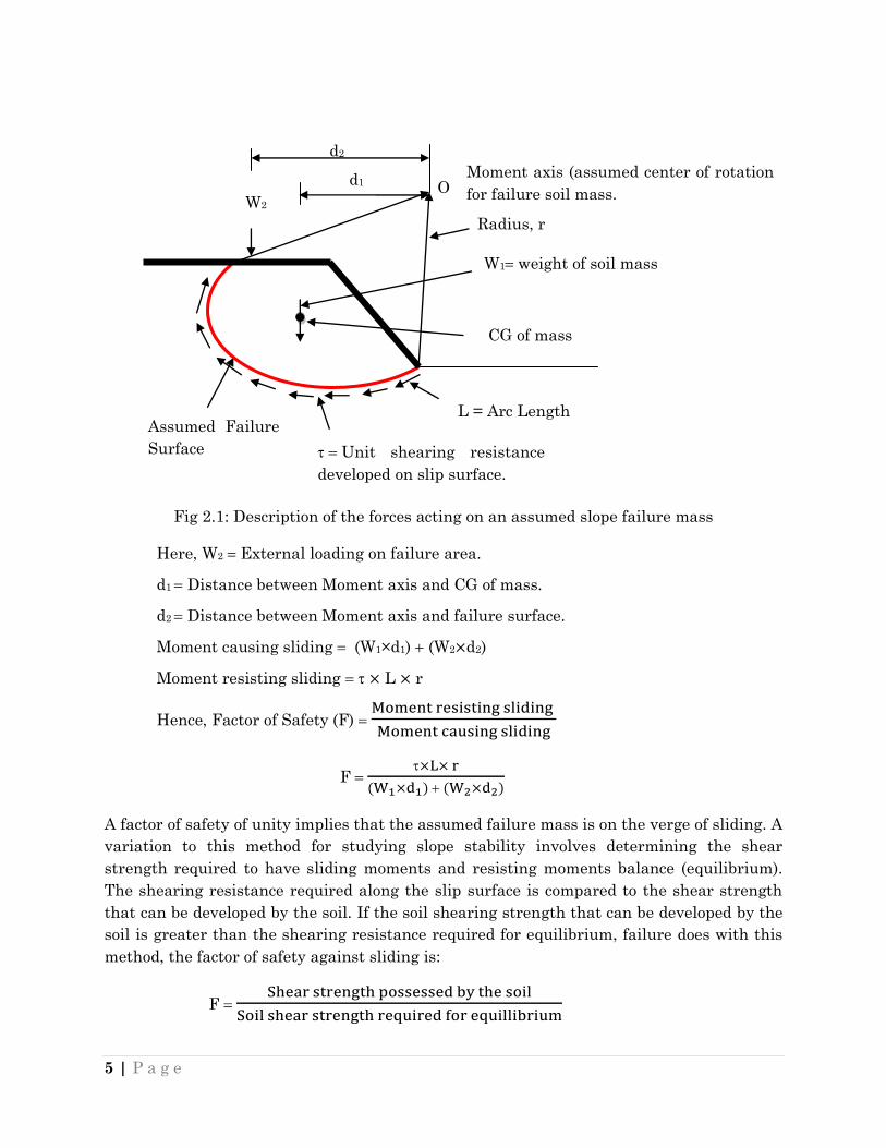
Fig 2.1: Description of the forces acting on an assumed slope failure mass
Here, W2 External loading on failure area.
d1 Distance between Moment axis and CG of mass.
d2 Distance between Moment axis and failure surface.
Moment causing sliding (W1×d1) (W2 d2)
Moment resisting sliding L r
Hence, Factor of Safety (F)
F
A factor of safety of unity implies that the assumed failure mass is on the verge of sliding. A
variation to this method for studying slope stability involves determining the shear
strength required to have sliding moments and resisting moments balance (equilibrium).
The shearing resistance required along the slip surface is compared to the shear strength
that can be developed by the soil. If the soil shearing strength that can be developed by the
soil is greater than the shearing resistance required for equilibrium, failure does with this
method, the factor of safety against sliding is:
F
Moment axis (assumed center of rotation
for failure soil mass. d1
W2
Unit shearing resistance
developed on slip surface.
Assumed Failure
Surface
CG of mass
W1weight of soil mass
L = Arc Length
6 | P a g e
The factor of safety indicated by this method is a value based on the soil's shear strength.
This method is used in most of the mathematical slope stability theories.
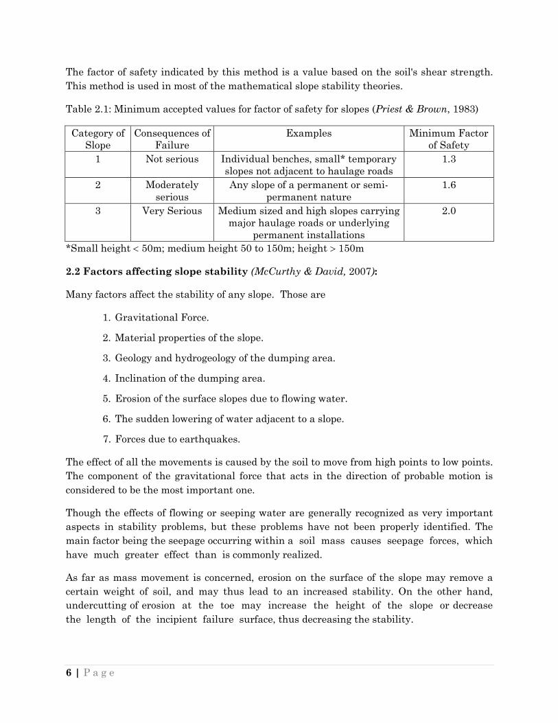
Table 2.1: Minimum accepted values for factor of safety for slopes (Priest & Brown, 1983)
Category of
Slope
Consequences of
Failure
Examples Minimum Factor
of Safety
1 Not serious Individual benches, small* temporary
slopes not adjacent to haulage roads
1.3
2 Moderately
serious
Any slope of a permanent or semi-
permanent nature
1.6
3 Very Serious Medium sized and high slopes carrying
major haulage roads or underlying
permanent installations
2.0
*Small height 50m; medium height 50 to 150m; height 150m
2.2 Factors affecting slope stability (McCurthy & David, 2007):
Many factors affect the stability of any slope. Those are
1. Gravitational Force.
2. Material properties of the slope.
3. Geology and hydrogeology of the dumping area.
4. Inclination of the dumping area.
5. Erosion of the surface slopes due to flowing water.
6. The sudden lowering of water adjacent to a slope.
7. Forces due to earthquakes.
The effect of all the movements is caused by the soil to move from high points to low points.
The component of the gravitational force that acts in the direction of probable motion is
considered to be the most important one.
Though the effects of flowing or seeping water are generally recognized as very important
aspects in stability problems, but these problems have not been properly identified. The
main factor being the seepage occurring within a soil mass causes seepage forces, which
have much greater effect than is commonly realized.
As far as mass movement is concerned, erosion on the surface of the slope may remove a
certain weight of soil, and may thus lead to an increased stability. On the other hand,
undercutting of erosion at the toe may increase the height of the slope or decrease
the length of the incipient failure surface, thus decreasing the stability.
7 | P a g e
Lowering of the ground-water surface or of a free water surface adjacent to the slope leads
to diminish the buoyancy of the soil which is in the effect an increase in the weight.
The increase in weight results in increase in the shearing stresses, whether or not the value
of permeability is lower. Practically no changes in volume will take place except at a certain
slope rate, and in spite of the increase of load, increase in strength may be inappreciable.
A decrease in the inter-granular pressure and increase in the neutral pressure accompany
shear force at a constant volume. A different condition may exist in which the soil mass
converts into a state of liquefaction and flows like liquid. This type of condition is likely to
be developed if the mass of the soil is subjected to vibration, possibly due to earthquake.
2.3 Sliding Block Analysis (McCurthy & David, 2007) (Fig 2.2 and 2.3)
Slopes consisting of the stratified materials and embankment structures on the constructed
on the stratified soil foundations can experience failure due to the sliding along one or more
of weaker layers. This type of failure often occur when changed conditions in an area cause
the susceptible layers to become exposed to, or saturated by, water. Exposure to moisture
can cause physical breakage and weakening of some earth materials, such as fine grained
sedimentary deposits, and saturation may cause reduction in stratum's shear strength
because of the increase in pore water pressures.
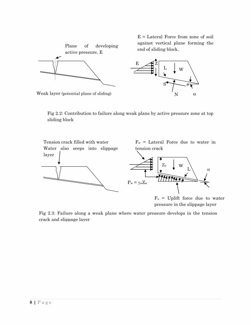
Where the potential for the occurrence of a block slide is under the study with no pore
pressure effect on the block, the factor of safety with regard to the shear strength of the soil
on the assumed sliding plane is given by,
Where E can be approximated as 0.25 soil Z2 for cohesion less soil and 0.5 soil Z2 for cohesive
soil if the formation of a tension crack along the top of the slope permits the development of
water pressure in the crack and the slippage zone, can be described as:
Where Fw is the force due water pressures in the tension crack, equal to 0.5water Z2water and
Fu = 0.5water Wwater L.
8 | P a g e
E Z
S a
N
W
L
E = Lateral Force from zone of soil
against vertical plane forming the
end of sliding block.
Weak layer (potential plane of sliding)
Plane of developing
active pressure, E
Fig 2.2: Contribution to failure along weak plane by active pressure zone at top
sliding block
W Zw L
Pw = wZw
Fw = Lateral Force due to water in
tension crack
Tension crack filled with water
Water also seeps into slippage
layer
Fu = Uplift force due to water
pressure in the slippage layer
Fig 2.3: Failure along a weak plane where water pressure develops in the tension
crack and slippage layer
9 | P a g e
Sections of several slopes have known to fail by translation along a weak foundation zone or
layer, the force responsible for movement responsible for movement resulting from lateral
soil pressure developed within the embankment itself. In the case of the earth dams, the
zone of the slippage may develop only after the dam has impounded water for a period, with
seepage through the eventual slippage zone being responsible for weakening to the extent
that a failure can occur.
The upstream as well as the downstream zones might be studied for stability. Though the
effect of water on the upstream embankment increases the weight „W‟, the lateral pressure
of the impounded water for a period opposes block translation. The uplift force is
considerably greater for upstream zones. Like other categories of sliding failures, it
determines the size and location of the section most susceptible to movement. It is typically
a trial and error procedure, because the most critical zone is not always obvious.
2.4 Phreatic Surface
The term phreatic is used in earth sciences in reference to matters relating to ground water
below the water table. The term 'phreatic surface' points the location where the pore water
pressure is under the condition of atmosphere (i.e. the pressure head is zero). Normally,
this surface normally coincides with the water table.
2.5 Effect of Tension Cracks
Developing Tension cracks along the face or crest of a slope (a condition most often antic-
ipated where cohesive soils exist) can influence stability. In an analysis, Soil possessing
zero shearing resistance is assigned to the section of slippage plane affected by tension
cracks. If the tension crack(s) could fill with water, a hydrostatic pressure distribution is
assumed to exist in the crack, and this pressure contributes to those forces and moments
acting to cause slope movement. Frequently, however, the computed factor of safety is less
influenced by the tension cracks, but it might be affected if tension cracks provide the
opportunity for water to reach otherwise buried earth layers whose strength may be
weakened by such exposure, an effect requiring consideration in the slope analysis.
2.6 Limit equilibrium analysis
Limit equilibrium method first defines a proposed slip surface, then the slip surface is
analyzed to obtain the factor of safety, which is defined as the ratio between forces
(moments or stresses) resisting instability of the mass and those that causing instability
(disturbing forces).
Two-dimensional sections are generally analyzed assuming plain strain conditions. The
assumption for these methods is that the linear (Mohr-Coulomb) or non-linear relationships
between shear strength and the normal stress on the failure surface governs the shear
strengths of the materials along the potential failure surface.
10 | P a g e
Functional slope design calculates the critical slip surface where the factor of safety is
found to be of lowest value. Computer programs can help locate failure surface using search
optimization techniques. The program analyzes the stability of different layered slopes,
embankments, and sheeting structures. Fast optimization of different slip surfaces (circular
& non-circular surfaces) provides the lowest factor of safety. External forces (Earthquake
effects, external loading, groundwater conditions, and stabilization forces) can also be
included. The software uses solution in accordance with various methods of slice.
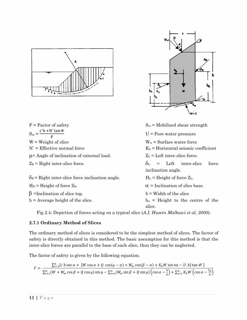
2.7 Methods of Slices (A.I. Husein Malkawi et al, 2000)
The problems associated with slope stability are statically indeterminate; hence some
simplified assumptions are made in order to determine a unique factor of safety. The
differences in assumptions lead to various methods of slices. The most popular methods are
on the procedures proposed by Fellenius, Bishop, Janbu and Spencer. These methods either
satisfy only overall moment or force equilibrium or both. The latter is applicable to failure
surface of any shape. Methods like the Ordinary and simplified Bishop Methods are
applicable to a circular slip surface, Janbu‟s method satisfies force equilibrium and is
applicable to both circular and non-circular shape. Spencer‟s method is applicable to both
moment and force equilibrium and it is applicable to failure surfaces of any shape. It is
considered as one of the accurate and rigorous methods for solving stability problems.
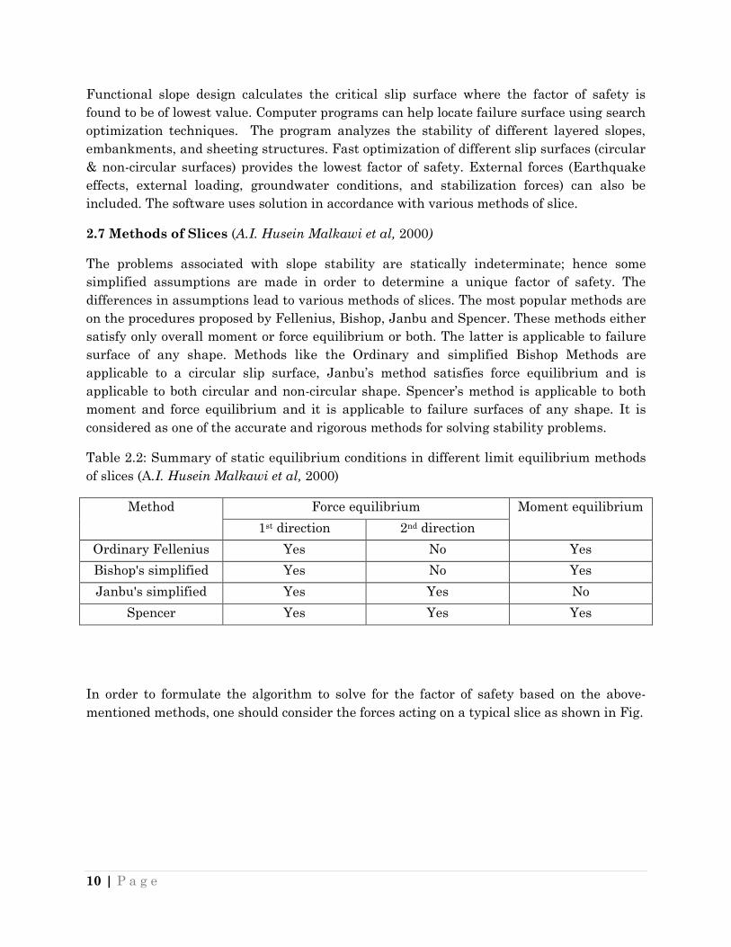
Table 2.2: Summary of static equilibrium conditions in different limit equilibrium methods
of slices (A.I. Husein Malkawi et al, 2000)
Method Force equilibrium Moment equilibrium
1st direction 2nd direction
Ordinary Fellenius Yes No Yes
Bishop's simplified Yes No Yes
Janbu's simplified Yes Yes No
Spencer Yes Yes Yes
In order to formulate the algorithm to solve for the factor of safety based on the above-
mentioned methods, one should consider the forces acting on a typical slice as shown in Fig.
11 | P a g e
F = Factor of safety Sm = Mobilized shear strength
Sm =
U = Pore water pressure
W = Weight of slice Ww = Surface water force
N` = Effective normal force Kh = Horizontal seismic coefficient
µ= Angle of inclination of external load. ZL = Left inter-slice force.
ZR = Right inter-slice force. L = Left inter-slice force
inclination angle.
R = Right inter-slice force inclination angle. HL = Height of force ZL.
HR = Height of force ZR. = Inclination of slice base.
=Inclination of slice top. b = Width of the slice
h = Average height of the slice. ha = Height to the centre of the
slice.
Fig 2.4: Depiction of forces acting on a typical slice (A.I. Husein Malkawi et al, 2000).
2.7.1 Ordinary Method of Slices
The ordinary method of slices is considered to be the simplest method of slices. The factor of
safety is directly obtained in this method. The basic assumption for this method is that the
inter-slice forces are parallel to the base of each slice, thus they can be neglected.
The factor of safety is given by the following equation.
∑ [ [ ] ]
∑ ∑ (
)
∑ (
)
12 | P a g e
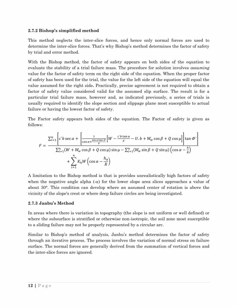
2.7.2 Bishop’s simplified method
This method neglects the inter-slice forces, and hence only normal forces are used to
determine the inter-slice forces. That‟s why Bishop‟s method determines the factor of safety
by trial and error method.
With the Bishop method, the factor of safety appears on both sides of the equation to
evaluate the stability of a trial failure mass. The procedure for solution involves assuming
value for the factor of safety term on the right side of the equation. When the proper factor
of safety has been used for the trial, the value for the left side of the equation will equal the
value assumed for the right side. Practically, precise agreement is not required to obtain a
factor of safety value considered valid for the assumed slip surface. The result is for a
particular trial failure mass, however and, as indicated previously, a series of trials is
usually required to identify the slope section and slippage plane most susceptible to actual
failure or having the lowest factor of safety.
The Factor safety appears both sides of the equation. The Factor of safety is given as
follows:
∑ [ [
*
+] ]
∑ ∑ (
)
∑ (
)
A limitation to the Bishop method is that is provides unrealistically high factors of safety
when the negative angle alpha (-) for the lower slope area slices approaches a value of
about 30°. This condition can develop where an assumed center of rotation is above the
vicinity of the slope's crest or where deep failure circles are being investigated.
2.7.3 Janbu’s Method
In areas where there is variation in topography (the slope is not uniform or well defined) or
where the subsurface is stratified or otherwise non-isotropic, the soil zone most susceptible
to a sliding failure may not be properly represented by a circular arc.
Similar to Bishop‟s method of analysis, Janbu‟s method determines the factor of safety
through an iterative process. The process involves the variation of normal stress on failure
surface. The normal forces are generally derived from the summation of vertical forces and
the inter-slice forces are ignored.
13 | P a g e
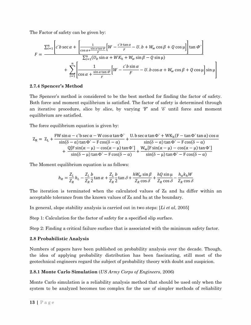
The Factor of safety can be given by:
∑ [ [
*
+] ]
∑
∑[
[
] ]
2.7.4 Spencer’s Method
The Spencer‟s method is considered to be the best method for finding the factor of safety.
Both force and moment equilibrium is satisfied. The factor of safety is determined through
an iterative procedure, slice by slice, by varying „F‟ and „‟ until force and moment
equilibrium are satisfied.
The force equilibrium equation is given by:
[ ]
[ ]
The Moment equilibrium equation is as follows:
The iteration is terminated when the calculated values of ZR and hR differ within an
acceptable tolerance from the known values of ZR and hR at the boundary.
In general, slope stability analysis is carried out in two steps: [Li et al, 2005]
Step 1: Calculation for the factor of safety for a specified slip surface.
Step 2: Finding a critical failure surface that is associated with the minimum safety factor.
2.8 Probabilistic Analysis
Numbers of papers have been published on probability analysis over the decade. Though,
the idea of applying probability distribution has been fascinating, still most of the
geotechnical engineers regard the subject of probability theory with doubt and suspicion.
2.8.1 Monte Carlo Simulation (US Army Corps of Engineers, 2006)
Monte Carlo simulation is a reliability analysis method that should be used only when the
system to be analyzed becomes too complex for the use of simpler methods of reliability
14 | P a g e
analysis, such as, the reliability index method. In Monte Carlo simulations, each random
variable is represented by a probability density function (PDF) and repeated conventional
analyses are made (iterations) by changing the values of the random variables (RV) using a
random number generator. To obtain an accurate Monte Carlo simulation solution, many
thousands of these conventional analyses must be performed. The simpler methods of
reliability analysis should be used whenever possible as the Monte Carlo simulation is
much more costly and time consuming.
Thus, in Monte Carlo simulation studies three steps are usually required, namely:
1. Determining the independent variable (input).
2. Transforming the input as independent variable (output).
3. Analyzing the output.
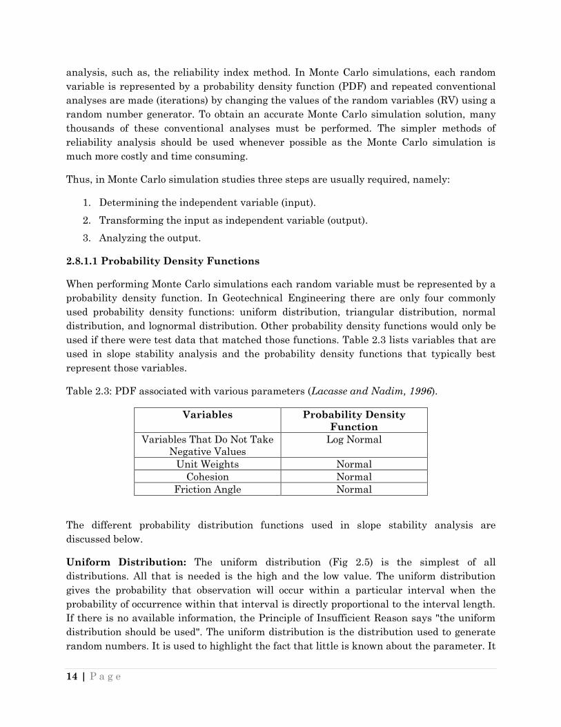
2.8.1.1 Probability Density Functions
When performing Monte Carlo simulations each random variable must be represented by a
probability density function. In Geotechnical Engineering there are only four commonly
used probability density functions: uniform distribution, triangular distribution, normal
distribution, and lognormal distribution. Other probability density functions would only be
used if there were test data that matched those functions. Table 2.3 lists variables that are
used in slope stability analysis and the probability density functions that typically best
represent those variables.
Table 2.3: PDF associated with various parameters (Lacasse and Nadim, 1996).
Variables Probability Density
Function
Variables That Do Not Take
Negative Values
Log Normal
Unit Weights Normal
Cohesion Normal
Friction Angle Normal
The different probability distribution functions used in slope stability analysis are
discussed below.
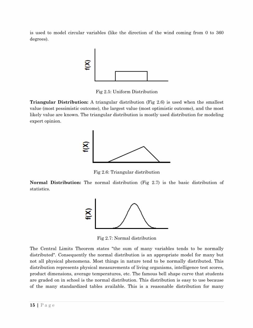
Uniform Distribution: The uniform distribution (Fig 2.5) is the simplest of all
distributions. All that is needed is the high and the low value. The uniform distribution
gives the probability that observation will occur within a particular interval when the
probability of occurrence within that interval is directly proportional to the interval length.
If there is no available information, the Principle of Insufficient Reason says "the uniform
distribution should be used". The uniform distribution is the distribution used to generate
random numbers. It is used to highlight the fact that little is known about the parameter. It
15 | P a g e
is used to model circular variables (like the direction of the wind coming from 0 to 360
degrees).
Fig 2.5: Uniform Distribution
Triangular Distribution: A triangular distribution (Fig 2.6) is used when the smallest
value (most pessimistic outcome), the largest value (most optimistic outcome), and the most
likely value are known. The triangular distribution is mostly used distribution for modeling
expert opinion.
Fig 2.6: Triangular distribution
Normal Distribution: The normal distribution (Fig 2.7) is the basic distribution of
statistics.
Fig 2.7: Normal distribution
The Central Limits Theorem states "the sum of many variables tends to be normally
distributed". Consequently the normal distribution is an appropriate model for many but
not all physical phenomena. Most things in nature tend to be normally distributed. This
distribution represents physical measurements of living organisms, intelligence test scores,
product dimensions, average temperatures, etc. The famous bell shape curve that students
are graded on in school is the normal distribution. This distribution is easy to use because
of the many standardized tables available. This is a reasonable distribution for many
16 | P a g e
things. If the normal distribution is used it is hard for someone to say that it is not the
correct distribution.
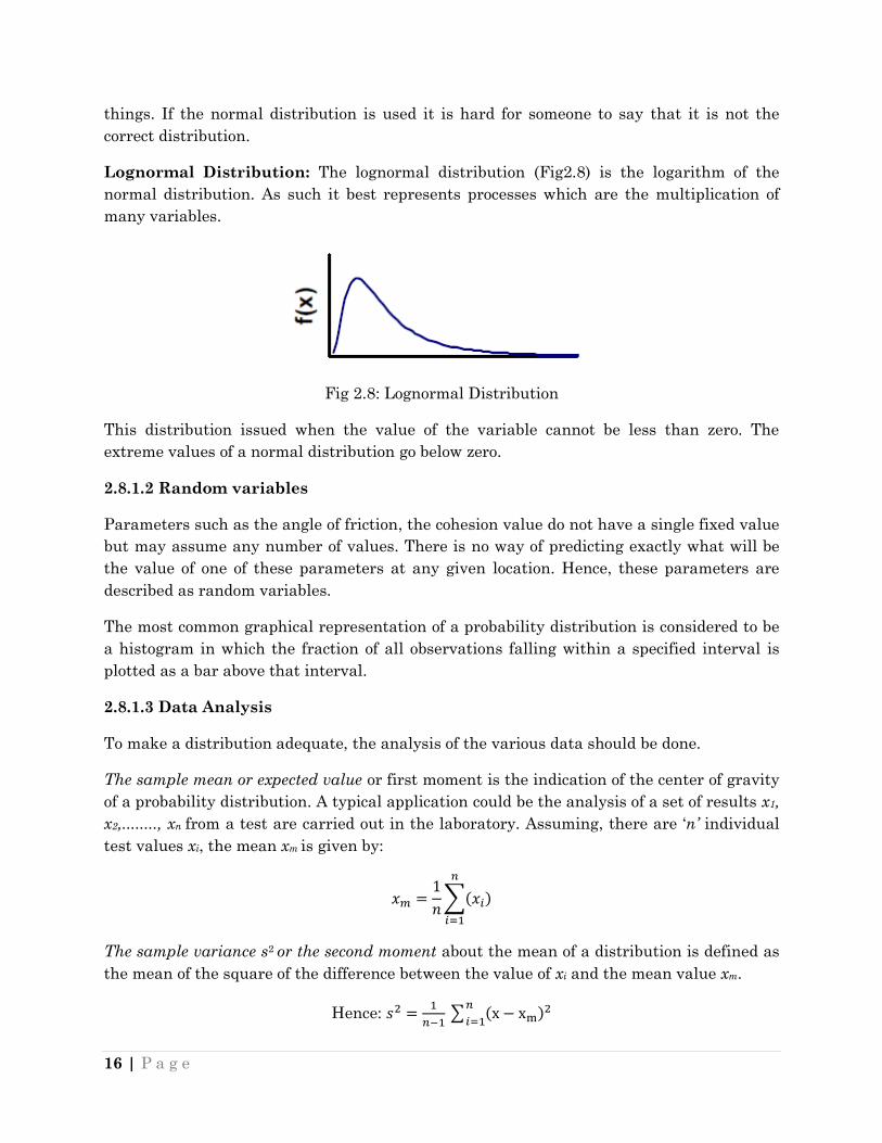
Lognormal Distribution: The lognormal distribution (Fig2.8) is the logarithm of the
normal distribution. As such it best represents processes which are the multiplication of
many variables.
Fig 2.8: Lognormal Distribution
This distribution issued when the value of the variable cannot be less than zero. The
extreme values of a normal distribution go below zero.
2.8.1.2 Random variables
Parameters such as the angle of friction, the cohesion value do not have a single fixed value
but may assume any number of values. There is no way of predicting exactly what will be
the value of one of these parameters at any given location. Hence, these parameters are
described as random variables.
The most common graphical representation of a probability distribution is considered to be
a histogram in which the fraction of all observations falling within a specified interval is
plotted as a bar above that interval.
2.8.1.3 Data Analysis
To make a distribution adequate, the analysis of the various data should be done.
The sample mean or expected value or first moment is the indication of the center of gravity
of a probability distribution. A typical application could be the analysis of a set of results x1,
x2,........, xn from a test are carried out in the laboratory. Assuming, there are „n’ individual
test values xi, the mean xm is given by:
∑
The sample variance s2 or the second moment about the mean of a distribution is defined as
the mean of the square of the difference between the value of xi and the mean value xm.
Hence:
∑

17 | P a g e
2.8.2 Methodology
Monte Carlo simulations, uses the same analysis method as conventional analysis does. It
runs each analysis multiple times. The random variables are represented as probability
density functions. The deterministic variables are represented as constants. Monte Carlo
simulation generally uses a random number generator to select the value of each random
variable using the probability density function specified for that random variable. For each
iteration (analysis), a factor of safety is calculated. Each factor of safety resulting from
iteration is counted to develop a probability density function for the factor of safety and to
determine the number of unsatisfactory performance events. The iterations are repeated
thousands of times until the process converges. From the probability density function for
the factor of safety or from the number of factors of safety counted that are less than one
divided by the number of iterations the percent of the factor of safeties less than one is
calculated to determine the probability of unsatisfactory performance which is considered
as the probability of failure of a particular number of simulations. To accomplish the many
thousands of iterations a computer program is needed.
Lacasse & Nadim et al (1996) proposed that usually normal distribution is used for various
soil properties.
A.I. Husein Malkawi et al (2000) proposed that the reliability index () and the probability
of failure (Pf) can be calculated using the safety factor probability distribution. This
approach can be applied to any method of slices, that uses limit equilibrium in the analysis
of slopes.
The uncertainty in slope stability is quantified by evaluating the reliability index, which is
defined as:
Where, ß is the reliability index, E(F) the expected value of the safety factor, and (F) is the
standard deviation.
The Monte Carlo Simulation for this project is done by using GALENA slope stability
system.
18 | P a g e
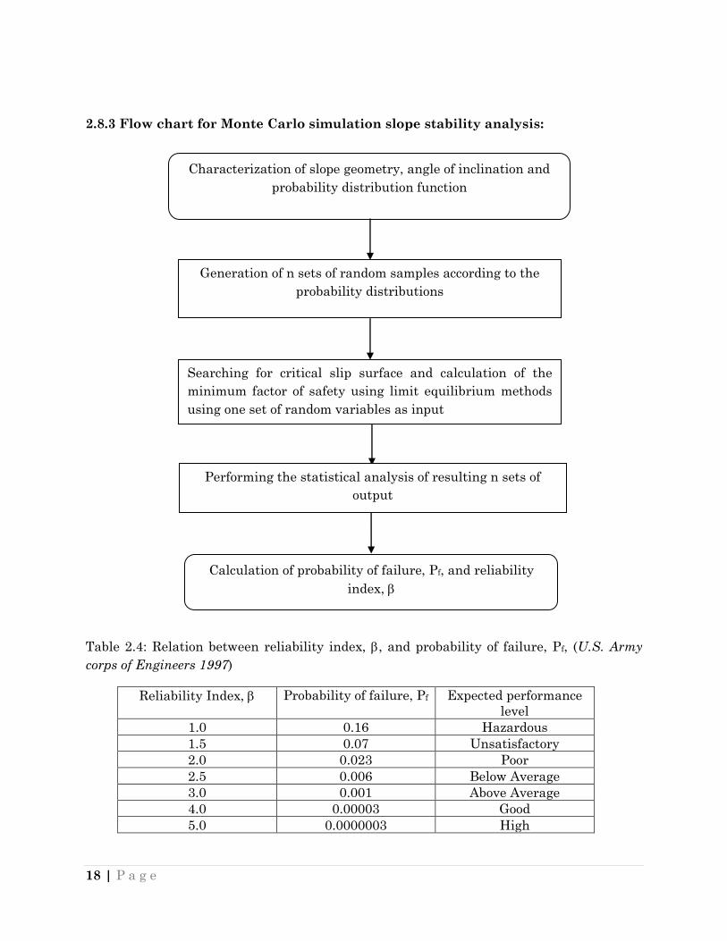
2.8.3 Flow chart for Monte Carlo simulation slope stability analysis:
Table 2.4: Relation between reliability index, , and probability of failure, Pf, (U.S. Army
corps of Engineers 1997)
Reliability Index, Probability of failure, Pf Expected performance
level
1.0 0.16 Hazardous
1.5 0.07 Unsatisfactory
2.0 0.023 Poor
2.5 0.006 Below Average
3.0 0.001 Above Average
4.0 0.00003 Good
5.0 0.0000003 High
Characterization of slope geometry, angle of inclination and
probability distribution function
Generation of n sets of random samples according to the
probability distributions
Searching for critical slip surface and calculation of the
minimum factor of safety using limit equilibrium methods
using one set of random variables as input
Performing the statistical analysis of resulting n sets of
output
Calculation of probability of failure, Pf, and reliability
index,

19 | P a g e
Wang et al (2011) reported that for a Pf level of 0.001, which corresponds to an expected
performance level “above average”. The sample size of direct Monte Carlo Simulation
should be greater than 10,000. As the deterministic slope stability analysis explicitly
searches a wide range of potential slip surfaces, it takes a considerable amount of time.
The randomness and uncertainty in the soil property are the most important factors that
may affect the reliability of the safety factor.
2.9 Slope Stability Analysis System – GALENA
GALENA is designed to be a simple, user-friendly yet very powerful, slope stability
software system. It was originally developed to satisfy the requirements of BHP (now
known as BHP Billiton) geotechnical engineers who realized there were many problems
with other slope stability analysis software systems available. Geotechnical engineering
very rarely gives one unique answer and extensive parametric studies are often required
before realistic results are obtained. GALENA enables such parametric studies to be
undertaken quickly and easily.
The GALENA system considers slope stability problems as they are largely encountered in
the field. That is, the overall geology generally remains the same; it is the slope surface that
requires change in many situations. In GALENA, the overall geology is defined for the
model, including the material properties. The defined slope surface then cuts through this
model, as a slope would be excavated in the real world. Material above the slope surface is
ignored since this has been removed or mined out. In this way, GALENA enables a large
number of analyses to be undertaken without the need to redefine the model each time.
Fig 2.9: A figure depicting an analysis in earlier version of GALENA

20 | P a g e
GALENA incorporates the Bishop Simplified, the Spencer-Wright and the Sarma methods
of analysis to determine the stability of slopes and excavations. The Bishop method is used
to determine the stability of circular failure surfaces, the Spencer-Wright method is
applicable for circular and non-circular failure surfaces, and the Sarma method is used for
problems where non-vertical slices are required, or is used for more complex stability
problems.
It is possible to analyze multi-layered slopes with tension cracks, earthquake forces,
externally distributed loads and forces, and water pressures from within or above the slope
(e.g. dams and river banks) including phreatic surfaces and piezometric pressures.
GALENA incorporates various techniques for locating the critical failure surface with user-
supplied restraints. Back analyses can also be performed to obtain critical material
strength parameters from known or assumed failure surfaces, and probability analyses
performed to gauge the likelihood of Factors of Safety being below values of interest, based
on expected material property variations.
Either effective or total stresses may be used on any material layer. For the total stress
case, the increase in undrained shear strength with depth can be simulated using
Skempton's relationship by simply entering the value of the plasticity index for that
material.
Probabilistic analysis can be readily undertaken using either defined material properties,
or defined mean values, and standard deviation for the production of density and
distribution plots.
GALENA allows shear strength to be defined using traditional c and phi values, the Hoek-
Brown (1983) failure criterion (m, s and UCS), or with shear/normal data from curves of
any shape.
2.9.1 Methods of Analysis
GALENA incorporates three different methods of slope stability analysis. These are:
i. BISHOP SIMPLIFIED METHOD - suitable for circular failure surfaces.
ii. SPENCER-WRIGHT METHOD - suitable for circular and non-circular failure
surfaces.
iii. SARMA METHOD - suitable for more complex problems particularly where non-
vertical slice boundaries (such as faults or discontinuities) are significant.
In most instances, slope stability problems can be analyzed with one of the above methods.
However, for complex slope stability problems where in-situ stresses are significant, it may
be more appropriate to use a stress analysis method such as finite element or finite
difference etc. Nevertheless, GALENA will provide rapid answers for most slope stability

21 | P a g e
problems and it has some features that are designed specifically for the practicing
geotechnical engineer, which are detailed within this Users‟ Guide.
GALENA calculates factor of safety through a surface which is most likely to fail in
comparison to other surfaces adjacent to it. It can also produce another 99 failure surfaces
which are likely to fail after this.
Fig 2.10: A program showing one critical failure surface through a slope
Fig 2.11: A program showing 99 critical failure surfaces through a slope.
22 | P a g e
2.9.2 Numerical Errors - Limit Equilibrium Methods of Analysis
For limit equilibrium analysis procedures, numerical errors are known to be associated
with the following cases:
a) Cohesive soil slopes with a shallow failure surface or where a high cohesive layer
exists along the upper portion of the failure surface. Negative stresses may be
generated towards the top of the failure surface.
b) Where a steeply dipping section of a circular surface is present in the toe region,
particularly when a relatively thin cohesion-less layer overlies a thicker layer of
weak clay. Similar problems may be encountered with non-circular failure surfaces
where a sub-horizontal surface is present at shallow depth and connected to the
ground (slope) surface by a steeply inclined section. Very large or negative stresses
may result under these conditions.
23 | P a g e
CHAPTER – 3
EXPERIMENTAL TECHNIQUES AND RESULTS
3.1 General Description of the Mine
The aim of the study is to investigate the existing status of slope of the mines. So, a nearby
operating mine was considered for investigation. Though the state Odisha is mineral rich,
deposits are mostly concentrated in the district of Keonjhar.
The region Keonjhar has a no of mines; particularly surface mines as a host of minerals
such as Iron, Manganese, Dolomite, etc. Many of these mines have private ownerships and
they hold limited lease area to operate the mine. The mine under investigation belongs to
Joda, Keonjhar District, Odisha which is about 141 miles from Bhubaneswar, the capital
city of the state in the eastern region of India, well connected by road to Keonjhar (80 Km)
to Barbil (35 Km) and Jamshedpur (180 Km). The production capacity of the mine is 2
million MT. The typical ores in this region are Haematite, Magnetite, Goethite and
Siderite. The major chemical composition of the iron ore produced here are Haematite
(Fe2O3), Magnetite (Fe3O4). The cut-off grade of Iron in the ore is 55%. Any materials
containing less than 55% of iron are considered as waste materials.
3.1.1 Mining
The method of working is opencast mechanized mining considering various technical
parameters like surface topography, continuation of iron deposit, quality variations, geo-
technical aspects, required rate of production etc. The deposit is mined by adopting 10.0 m
bench height and with width more than the height of benches i.e. more than 10 m, with an
ultimate pit slope of 45°. The transportation of the materials is done using Shovel-Dumper
combination.
3.1.2 Transportation
The blasted materials are transported using shovel-dumper combination. The same is the
case for waste materials. Dumpers of 25T and 35T capacity are used for this very purpose.
3.1.3 Dumping
The waste generated in the years of the plan period was accommodated in a waste dump
situated in the Western part of the mine. The dump is situated to be more or less 1 km from
the mine. Area available for dumping is 375m 225m. The waste materials are dumped
with the use of dumper capacity of 25 Tons. The materials are compacted through the
conventional mechanism. The present height of the dump is about 32m.

24 | P a g e
Fig 3.1: Plan of the Waste dump of the mine under study
Section AA‟ Section CC‟
Section BB‟ Section DD‟
The plan of the waste dump of the mine is shown in the fig 3.1. As no mineral processing
plant is present, the sub-grade materials are stacked in the form of a dump, which is also
known as a sub-grade stack yard.
The dumpers usually forge the load and dump at the central position of the area and move
towards the boundary. Dozers then spread and level the waste.
3.2 Field Observations
The investigation involves determination of geo-technical parameters, study of mine plans,
dumping process, etc. So to collect data, a no of visits were incurred to the mine including
dump site and the following observations are drawn.
25 | P a g e
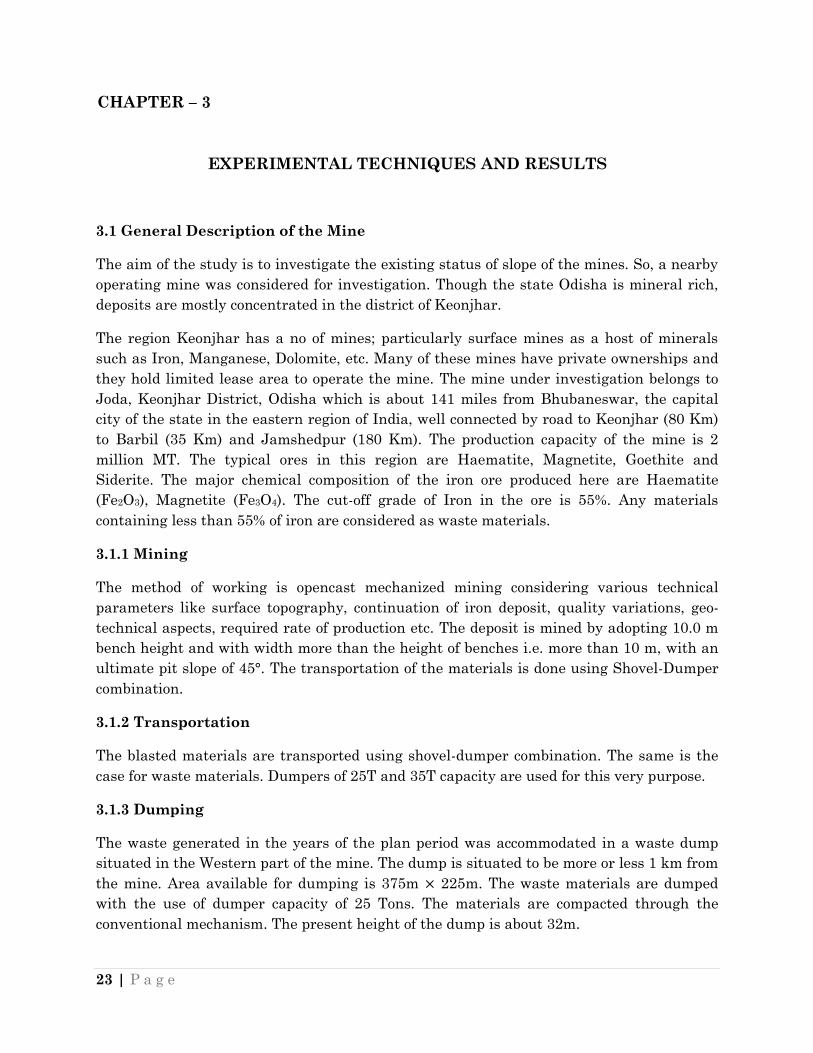
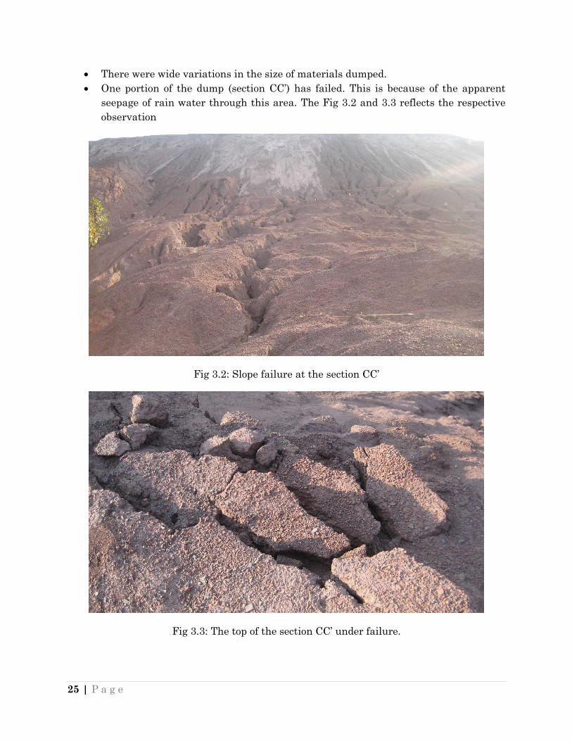
There were wide variations in the size of materials dumped.
One portion of the dump (section CC‟) has failed. This is because of the apparent
seepage of rain water through this area. The Fig 3.2 and 3.3 reflects the respective
observation
Fig 3.2: Slope failure at the section CC‟
Fig 3.3: The top of the section CC‟ under failure.
26 | P a g e
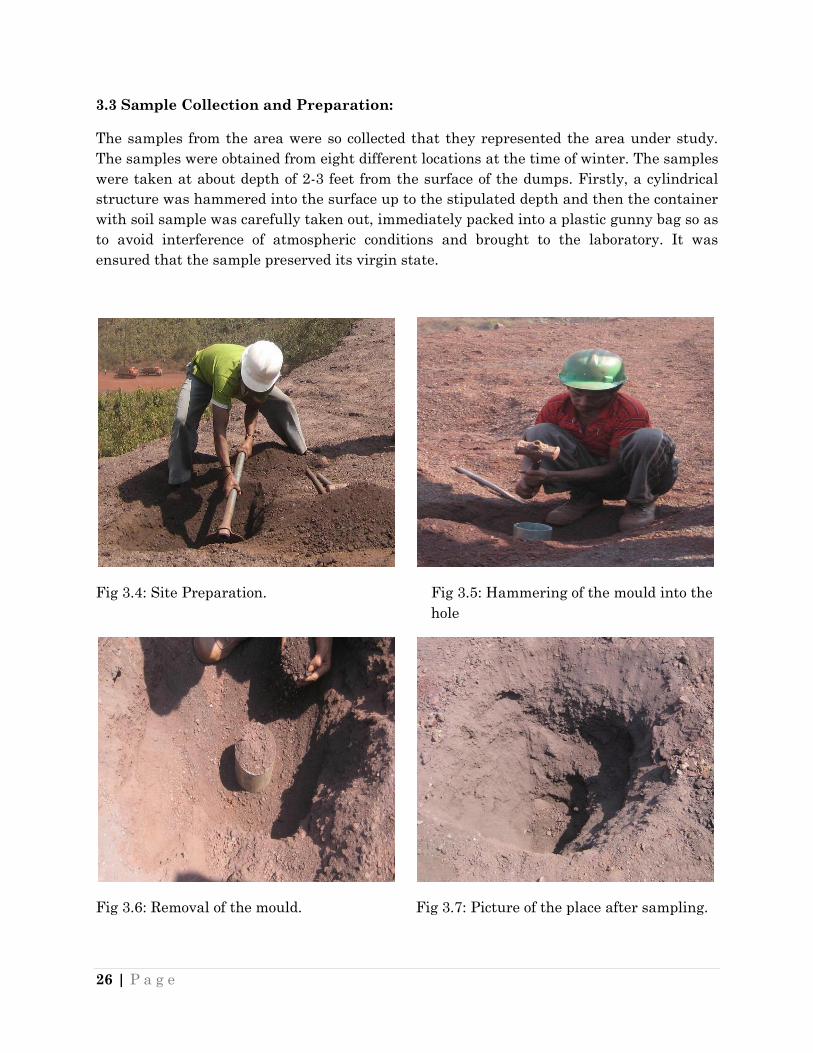
3.3 Sample Collection and Preparation:
The samples from the area were so collected that they represented the area under study.
The samples were obtained from eight different locations at the time of winter. The samples
were taken at about depth of 2-3 feet from the surface of the dumps. Firstly, a cylindrical
structure was hammered into the surface up to the stipulated depth and then the container
with soil sample was carefully taken out, immediately packed into a plastic gunny bag so as
to avoid interference of atmospheric conditions and brought to the laboratory. It was
ensured that the sample preserved its virgin state.
Fig 3.4: Site Preparation. Fig 3.5: Hammering of the mould into the
hole
Fig 3.6: Removal of the mould. Fig 3.7: Picture of the place after sampling.
27 | P a g e
Then the samples were sieved to required sizes (3.75mm) and stored in air tight polythene
packets. The packets were stored in air tight containers for further use in experimentation.
3.4 Experimental Methods:
The Geotechnical parameters needed for the stability analysis are:
1. Unit weight „‟.
2. Cohesion „c‟
3. Friction angle „‟ (UU test)
4. Angle of repose „ß‟
5. Pore water pressure.
But because of the unavailability of the instruments in the laboratory, only Proctor
compaction test and Tri-axial test of the samples were carried out.
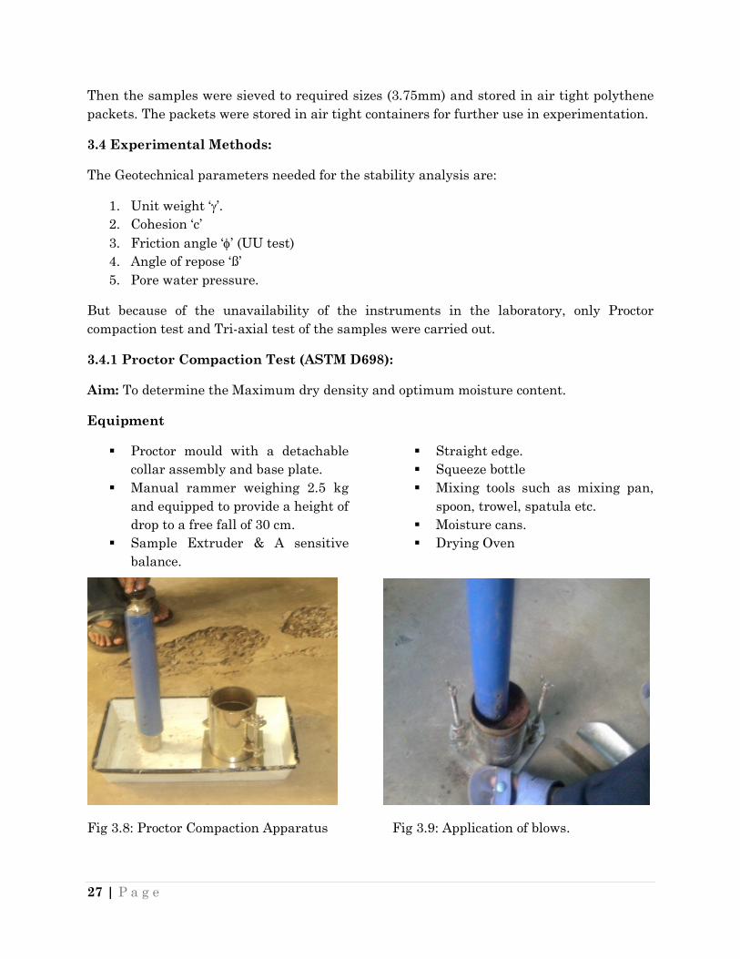
3.4.1 Proctor Compaction Test (ASTM D698):
Aim: To determine the Maximum dry density and optimum moisture content.
Equipment
Proctor mould with a detachable
collar assembly and base plate.
Manual rammer weighing 2.5 kg
and equipped to provide a height of
drop to a free fall of 30 cm.
Sample Extruder & A sensitive
balance.
Straight edge.
Squeeze bottle
Mixing tools such as mixing pan,
spoon, trowel, spatula etc.
Moisture cans.
Drying Oven
Fig 3.8: Proctor Compaction Apparatus Fig 3.9: Application of blows.
28 | P a g e
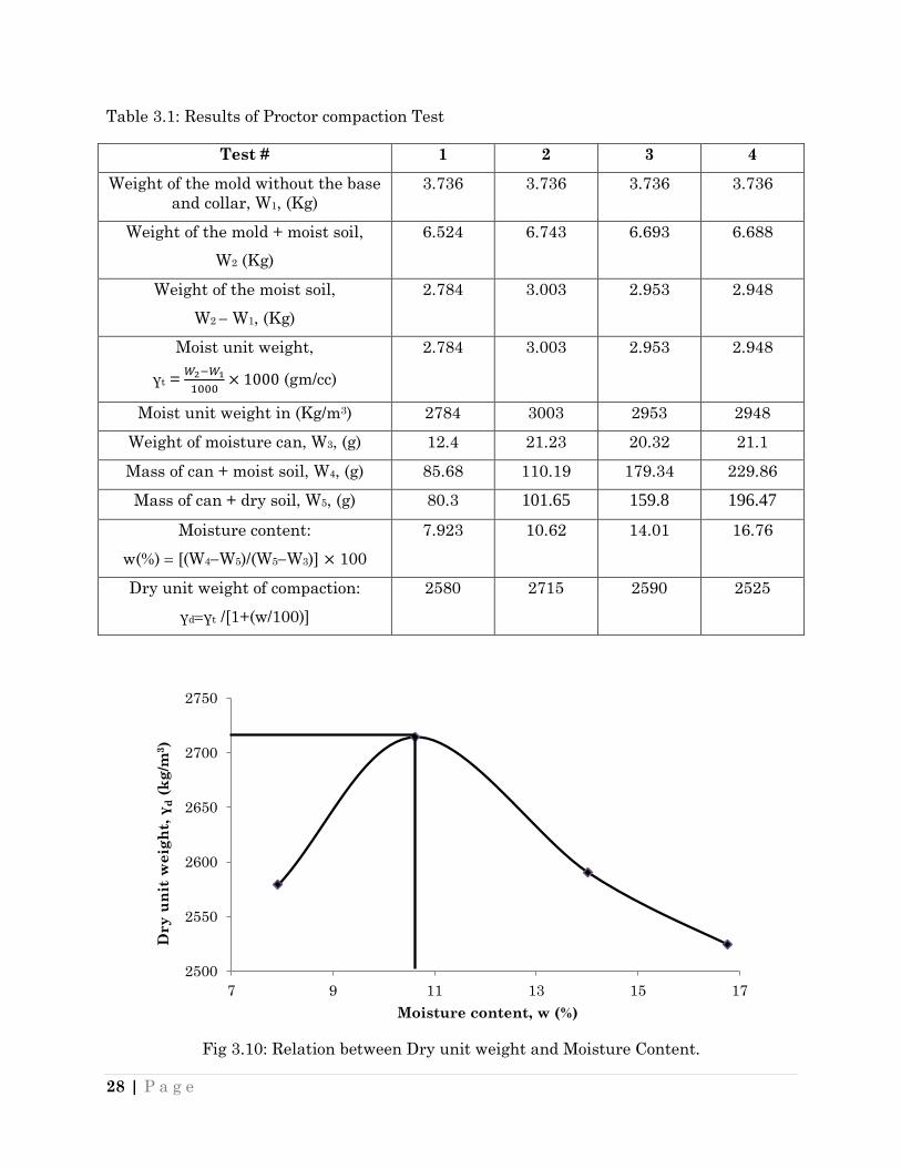
Table 3.1: Results of Proctor compaction Test
Test # 1 2 3 4
Weight of the mold without the base
and collar, W1, (Kg)
3.736 3.736 3.736 3.736
Weight of the mold + moist soil,
W2 (Kg)
6.524 6.743 6.693 6.688
Weight of the moist soil,
W2 W1, (Kg)
2.784 3.003
2.953
2.948
Moist unit weight,
γt =
(gm/cc)
2.784 3.003
2.953
2.948
Moist unit weight in (Kg/m3) 2784 3003 2953 2948
Weight of moisture can, W3, (g) 12.4 21.23 20.32 21.1
Mass of can + moist soil, W4, (g) 85.68 110.19 179.34 229.86
Mass of can + dry soil, W5, (g) 80.3 101.65 159.8 196.47
Moisture content:
w(%) [(W4W5)/(W5W3)] 100
7.923 10.62 14.01 16.76
Dry unit weight of compaction:
γdγt /[1+(w/100)]
2580 2715 2590 2525
Fig 3.10: Relation between Dry unit weight and Moisture Content.
2500
2550
2600
2650
2700
2750
7 9 11 13 15 17
Dry
un
it w
eig
ht,
γd (
kg
/m3)
Moisture content, w (%)

29 | P a g e
From the graph, it can be found that:
Maximum Dry Density = 2715 kg/m3
Optimum moisture content = 10.62%
3.4.2 Tri-Axial Test (ASTM D2850):
This test method covers determination of the strength and stress-strain relationships of a
cylindrical specimen of either undisturbed or remolded cohesive soil. Specimens are
subjected to a confining fluid pressure in a triaxial chamber. No drainage of the specimen is
permitted during the test. The specimen is sheared in compression without drainage at a
constant rate of axial deformation (strain controlled).
This test method provides data for determining undrained strength properties and stress-
strain relations for soils. This test method provides for the measurement of the total
stresses applied to the specimen, that is, the stresses are not corrected for pore-water
pressure.
Apparatus
For conducting the test, the testing system consists of the following five major functional
components:
a) A system to house the sample, that is, a triaxial cell;
b) A system to apply cell pressure and maintain it at a constant magnitude;
c) A system to apply additional axial stress;
d) A system to measure pore water pressure; and
e) A system to measure changes of volume of the soil sample.
Elements Used within the Triaxial Cell
The Tri-axial Test may be programmed so as to allow or exclude the hydraulic connection
between the inside of the sample with the ambient outside the tri-axial cell or with special
measuring instruments. Such connections might require the use of special drainage
mediums around the sample, in particular: Porous Discs on the top and bottom of the
sample and Filter Drains around its sides. However, when the sample has to be isolated,
the bottom porous disc has to be replaced by an impermeable Base Disc whilst the upper
porous disc is removed. In each case the sample is placed on a Pedestal and a Top Cap is
placed on top of the sample. These elements will have the same diameter as the sample. To
make the sample isolated from the water within the triaxial cell, it is covered with a very
thin Membrane made of natural rubber (of appropriate diameter) which is placed over the
sample using a Suction Membrane Stretcher and a water-tight fit is guaranteed at the
junction with the pedestal and top cap by using Sealing Rings of appropriate diameter.
30 | P a g e
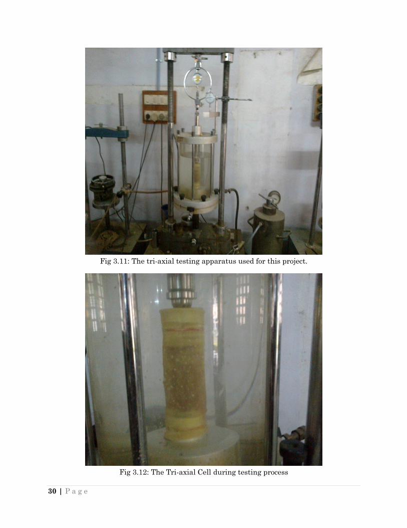
Fig 3.11: The tri-axial testing apparatus used for this project.
Fig 3.12: The Tri-axial Cell during testing process
31 | P a g e
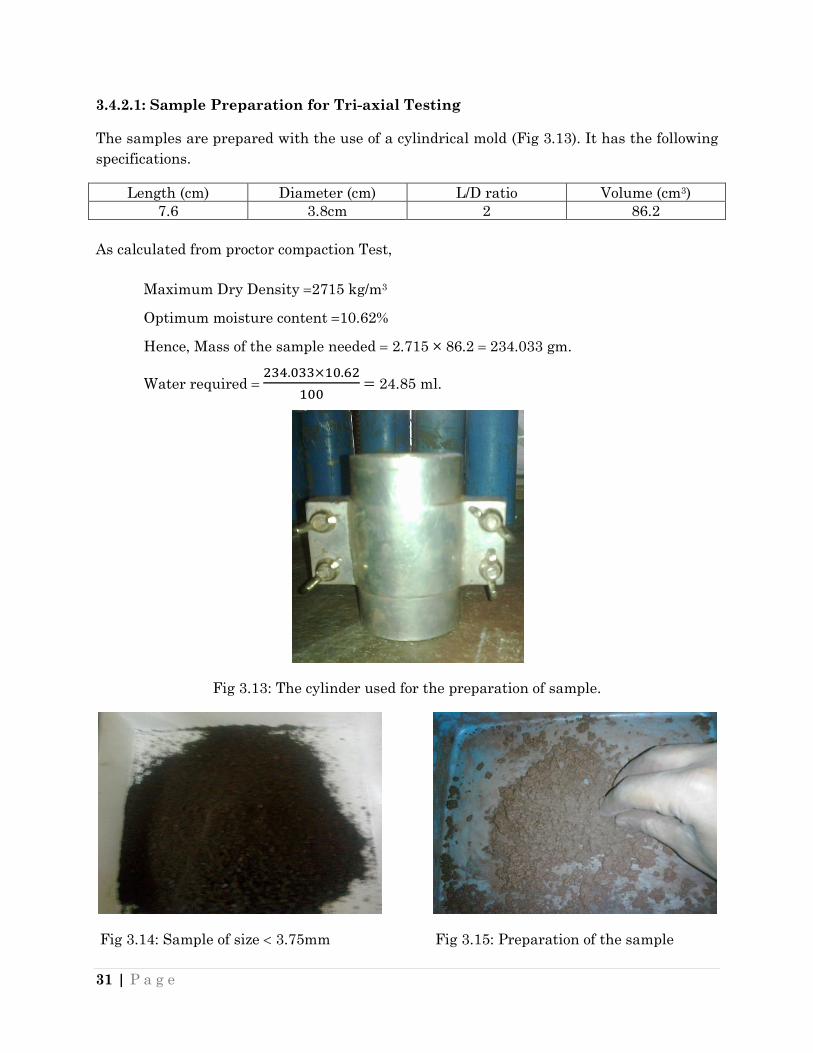
3.4.2.1: Sample Preparation for Tri-axial Testing
The samples are prepared with the use of a cylindrical mold (Fig 3.13). It has the following
specifications.
Length (cm) Diameter (cm) L/D ratio Volume (cm3)
7.6 3.8cm 2 86.2
As calculated from proctor compaction Test,
Maximum Dry Density 2715 kg/m3
Optimum moisture content 10.62%
Hence, Mass of the sample needed 2.715 × 86.2 234.033 gm.
Water required
24.85 ml.
Fig 3.13: The cylinder used for the preparation of sample.
Fig 3.14: Sample of size 3.75mm Fig 3.15: Preparation of the sample
32 | P a g e
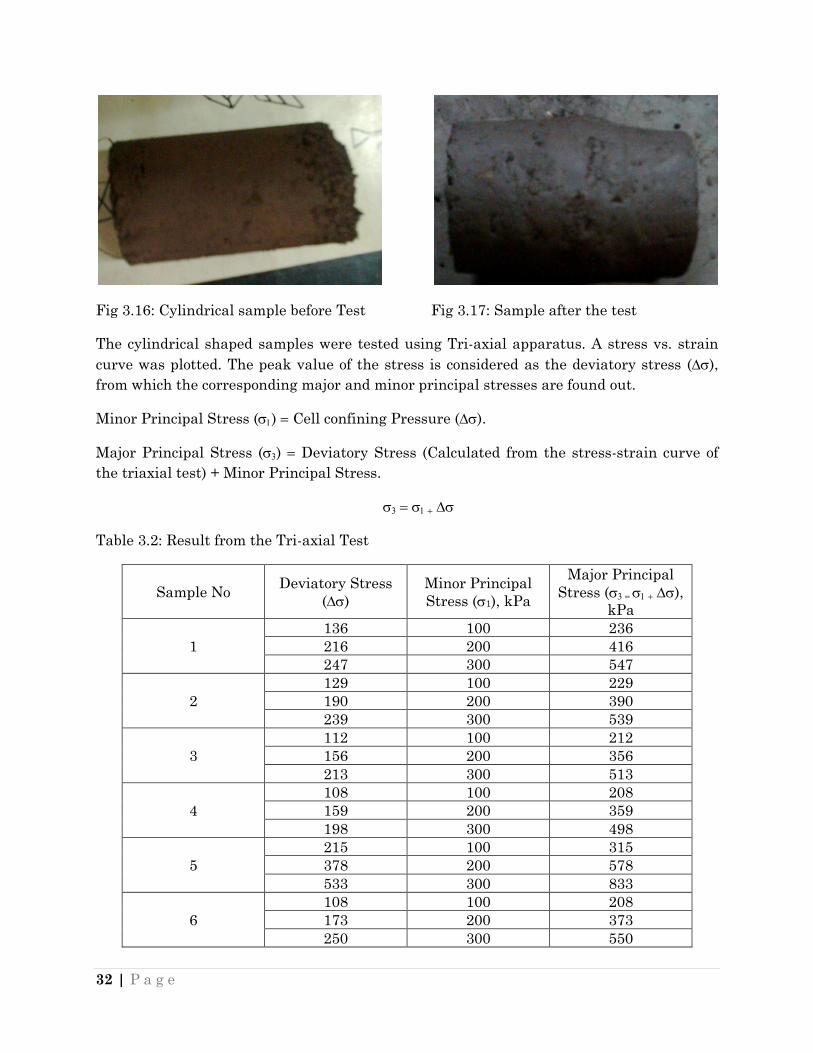
Fig 3.16: Cylindrical sample before Test Fig 3.17: Sample after the test
The cylindrical shaped samples were tested using Tri-axial apparatus. A stress vs. strain
curve was plotted. The peak value of the stress is considered as the deviatory stress ( ),
from which the corresponding major and minor principal stresses are found out.
Minor Principal Stress ( ) Cell confining Pressure ( ).
Major Principal Stress ( ) Deviatory Stress (Calculated from the stress-strain curve of
the triaxial test) + Minor Principal Stress.
Table 3.2: Result from the Tri-axial Test
Sample No Deviatory Stress
( )
Minor Principal
Stress ( 1), kPa
Major Principal
Stress ( ),
kPa
1
136 100 236
216 200 416
247 300 547
2
129 100 229
190 200 390
239 300 539
3
112 100 212
156 200 356
213 300 513
4
108 100 208
159 200 359
198 300 498
5
215 100 315
378 200 578
533 300 833
6
108 100 208
173 200 373
250 300 550
33 | P a g e
7
188 100 288
380 200 580
512 300 812
8
236 100 336
389 200 589
501 300 801
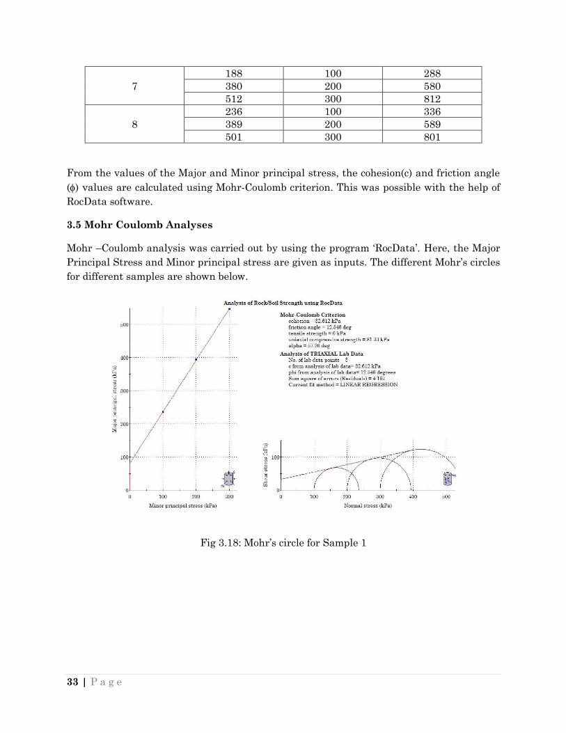
From the values of the Major and Minor principal stress, the cohesion(c) and friction angle
() values are calculated using Mohr-Coulomb criterion. This was possible with the help of
RocData software.
3.5 Mohr Coulomb Analyses
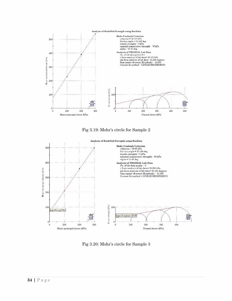
Mohr –Coulomb analysis was carried out by using the program „RocData‟. Here, the Major
Principal Stress and Minor principal stress are given as inputs. The different Mohr‟s circles
for different samples are shown below.
Fig 3.18: Mohr‟s circle for Sample 1
34 | P a g e
Fig 3.19: Mohr‟s circle for Sample 2
Fig 3.20: Mohr‟s circle for Sample 3
35 | P a g e
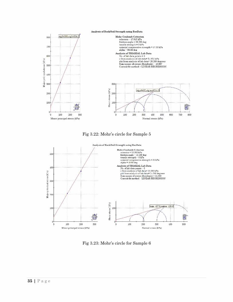
Fig 3.22: Mohr‟s circle for Sample 5
Fig 3.23: Mohr‟s circle for Sample 6
36 | P a g e
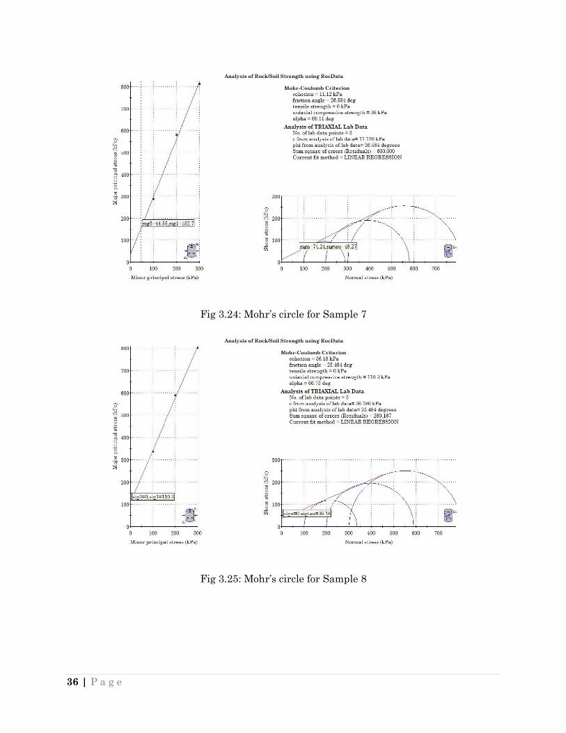
Fig 3.24: Mohr‟s circle for Sample 7
Fig 3.25: Mohr‟s circle for Sample 8
37 | P a g e
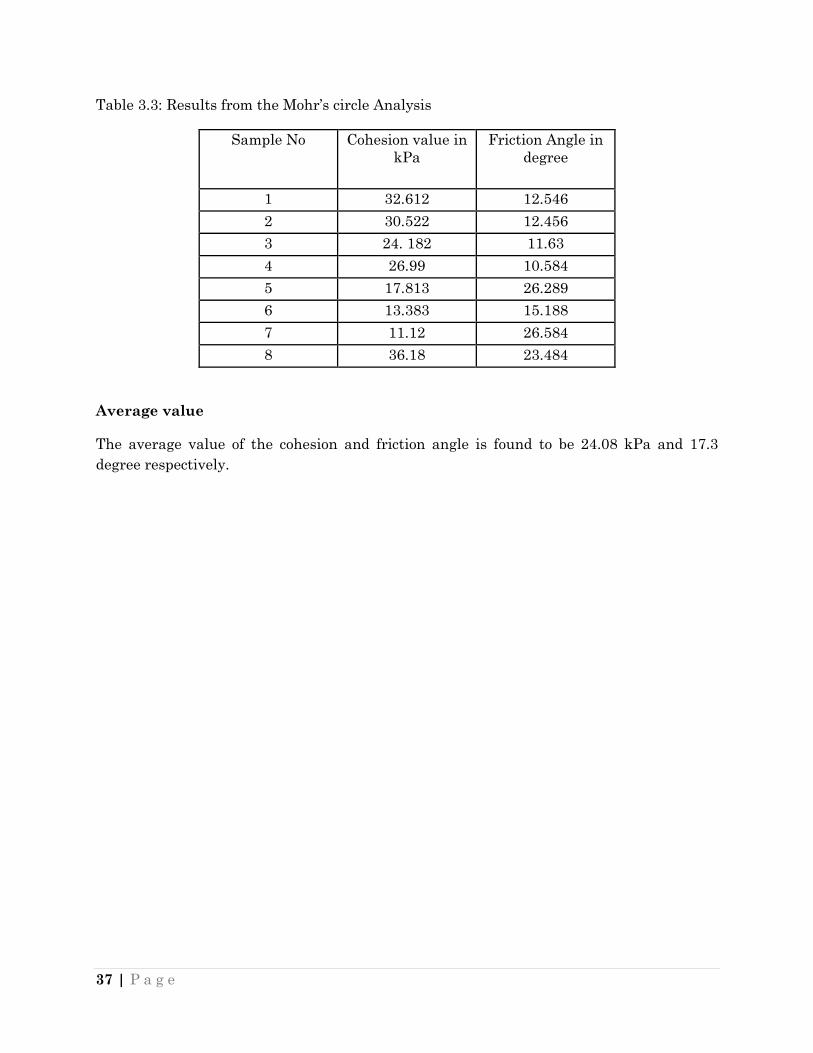
Table 3.3: Results from the Mohr‟s circle Analysis
Sample No Cohesion value in
kPa
Friction Angle in
degree
1 32.612 12.546
2 30.522 12.456
3 24. 182 11.63
4 26.99 10.584
5 17.813 26.289
6 13.383 15.188
7 11.12 26.584
8 36.18 23.484
Average value
The average value of the cohesion and friction angle is found to be 24.08 kPa and 17.3
degree respectively.
38 | P a g e
CHAPTER – 4
ANALYSIS
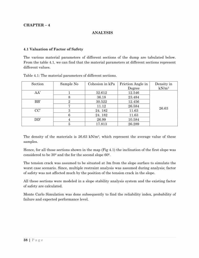
4.1 Valuation of Factor of Safety
The various material parameters of different sections of the dump are tabulated below.
From the table 4.1, we can find that the material parameters at different sections represent
different values.
Table 4.1: The material parameters of different sections.
Section Sample No Cohesion in kPa Friction Angle in
Degree
Density in
kN/m3
AA‟ 1 32.612 12.546
26.63
8 36.18 23.484
BB‟ 2 30.522 12.456
7 11.12 26.584
CC‟ 3 24. 182 11.63
6 24. 182 11.63
DD‟ 4 26.99 10.584
5 17.813 26.289
The density of the materials is 26.63 kN/m3, which represent the average value of these
samples.
Hence, for all those sections shown in the map (Fig 4.1) the inclination of the first slope was
considered to be 300 and the for the second slope 600.
The tension crack was assumed to be situated at 3m from the slope surface to simulate the
worst case scenario. Since, multiple restraint analysis was assumed during analysis; factor
of safety was not affected much by the position of the tension crack in the slope.
All these sections were modeled in a slope stability analysis system and the existing factor
of safety are calculated.
Monte Carlo Simulation was done subsequently to find the reliability index, probability of
failure and expected performance level.
39 | P a g e
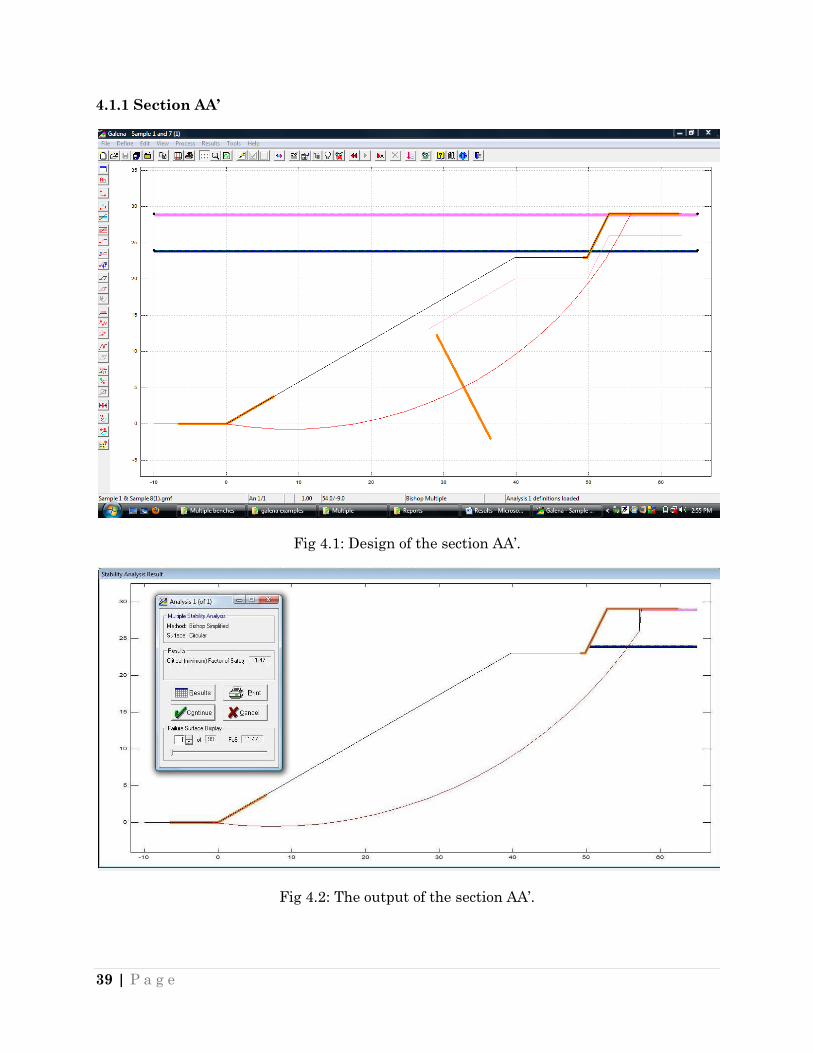
4.1.1 Section AA’
Fig 4.1: Design of the section AA‟.
Fig 4.2: The output of the section AA‟.
40 | P a g e
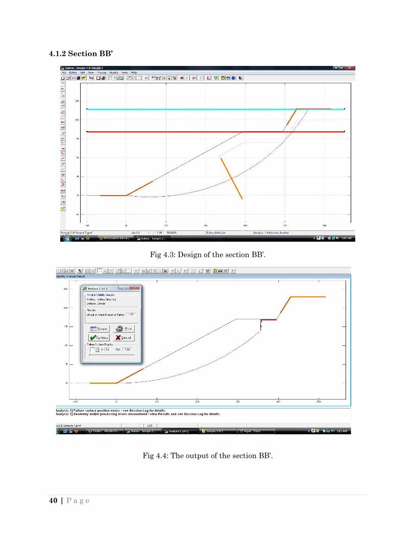
4.1.2 Section BB’
Fig 4.3: Design of the section BB‟.
Fig 4.4: The output of the section BB‟.
41 | P a g e
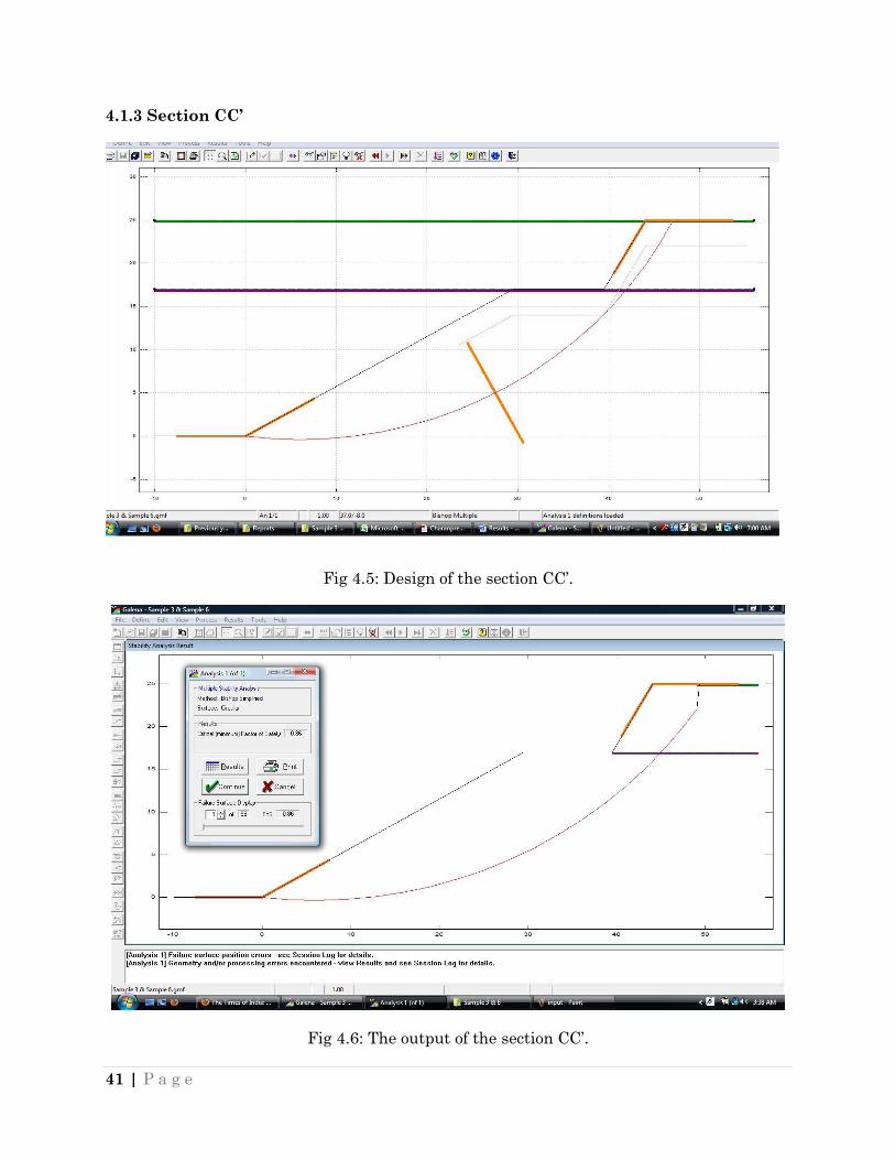
4.1.3 Section CC’
Fig 4.5: Design of the section CC‟.
Fig 4.6: The output of the section CC‟.
42 | P a g e
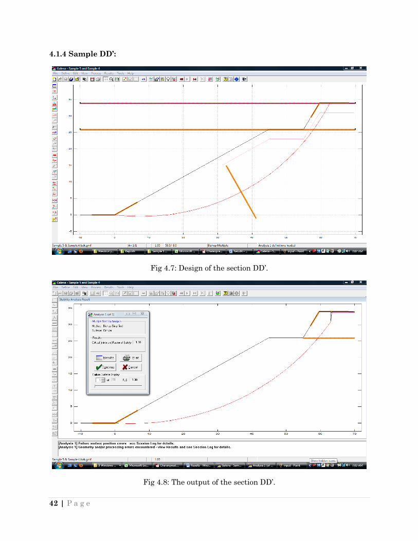
4.1.4 Sample DD’:
Fig 4.7: Design of the section DD‟.
Fig 4.8: The output of the section DD‟.

43 | P a g e
Table 4.2: FOS of different sections of the dump.
Section Factor of Safety Comments on the
stability
AA‟ 1.47 Stable
BB‟ 1.4 Stable
CC‟ 0.86 Unstable
DD‟ 1.3 Stable
From the analysis, it is evident that, the slope representing the section CC‟ is unstable. Figs
(3.2 & 3.3) show the failure of the slope. This is because the percolation of the rain water
through the slope.
4.2 Monte Carlo Simulation
The sample no 5, 6, 7 and 8 were collected from the first bench (Bench A) and the sample no
1, 2, 3 and 4 were collected from the second bench (Bench B).
Table 4.3: Characterization of fixed parameters
Slope A B
Bench Height (m) 21 7
Angle of Inclination (degree) 30 60
4.2.1 Material Parameters
Bench – A:
Mean value of Cohesion = 19.62
Standard deviation = 11.38
Mean value of Angle of Friction = 22.9
Standard deviation = 5.31
Bench - A
Fig 4.9: Normal Distribution curves for Cohesion and Angle of Friction
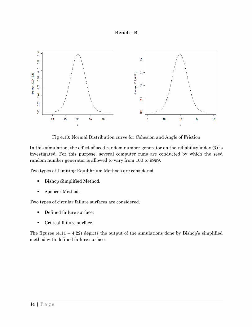
Bench – B:
Mean value of Cohesion = 30.04
Standard deviation = 2.84
Mean value of Angle of Friction = 11.9
Standard deviation = 0.911
44 | P a g e
Bench - B
Fig 4.10: Normal Distribution curve for Cohesion and Angle of Friction
In this simulation, the effect of seed random number generator on the reliability index () is
investigated. For this purpose, several computer runs are conducted by which the seed
random number generator is allowed to vary from 100 to 9999.
Two types of Limiting Equilibrium Methods are considered.
Bishop Simplified Method.
Spencer Method.
Two types of circular failure surfaces are considered.
Defined failure surface.
Critical failure surface.
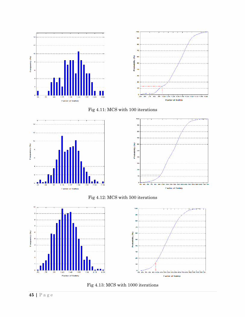
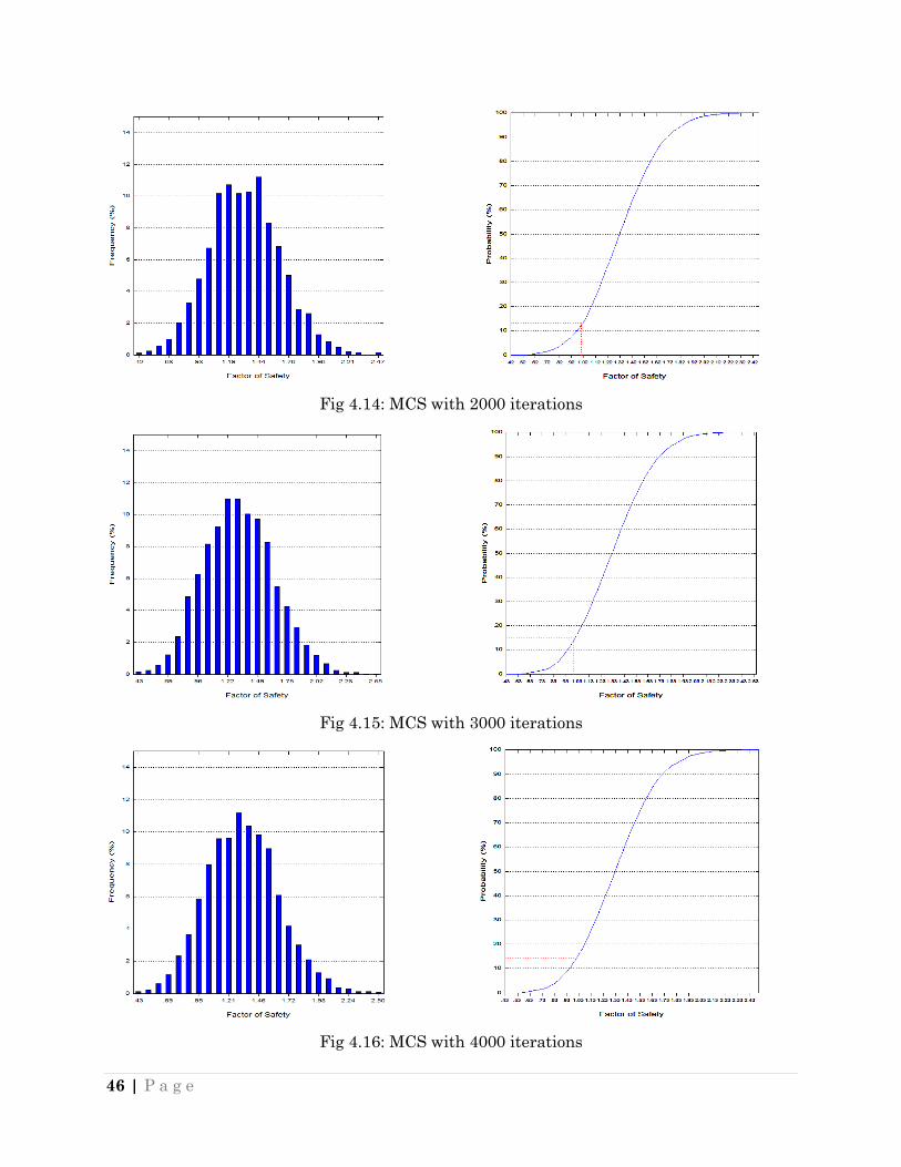
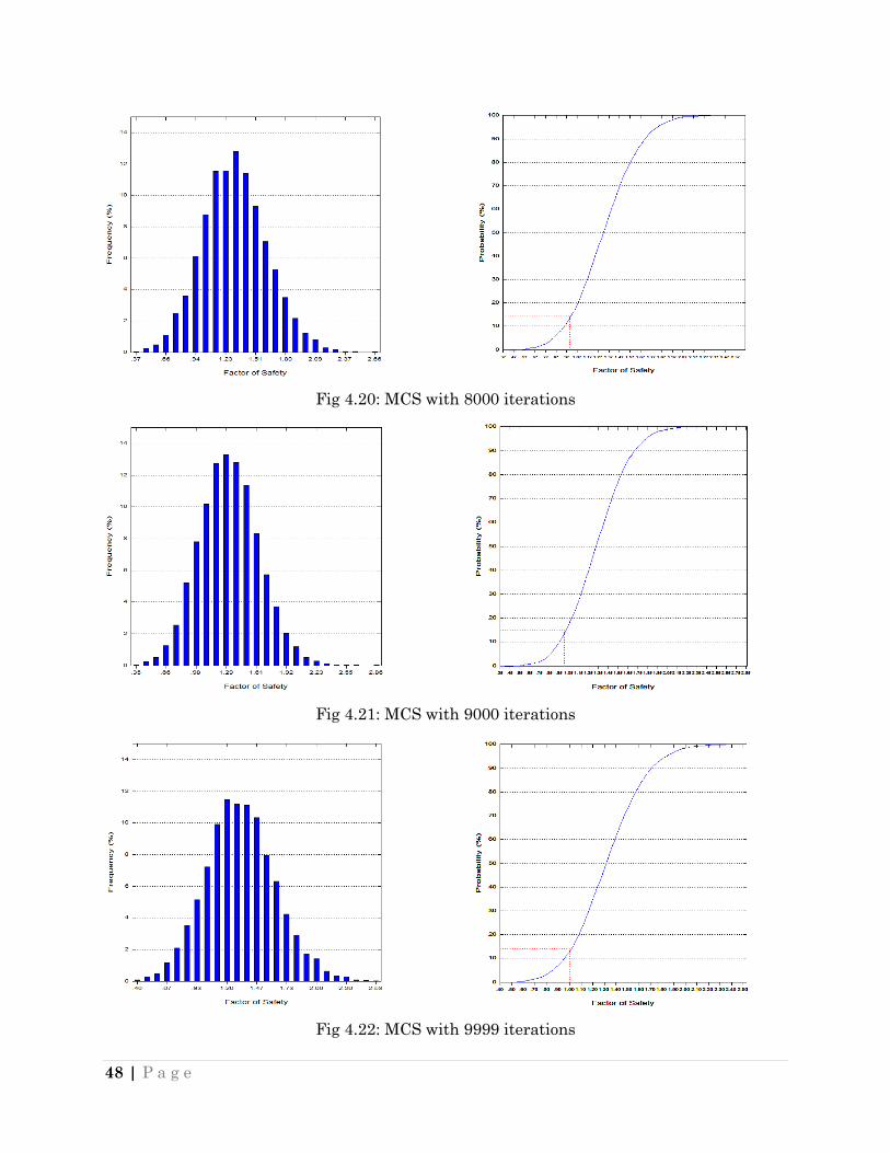
The figures (4.11 – 4.22) depicts the output of the simulations done by Bishop‟s simplified
method with defined failure surface.
45 | P a g e
Fig 4.11: MCS with 100 iterations
Fig 4.12: MCS with 500 iterations
Fig 4.13: MCS with 1000 iterations
46 | P a g e
Fig 4.14: MCS with 2000 iterations
Fig 4.15: MCS with 3000 iterations
Fig 4.16: MCS with 4000 iterations

47 | P a g e
Fig 4.17: MCS with 5000 iterations
Fig 4.18: MCS with 6000 iterations
Fig 4.19: MCS with 7000 iterations
48 | P a g e
Fig 4.20: MCS with 8000 iterations
Fig 4.21: MCS with 9000 iterations
Fig 4.22: MCS with 9999 iterations
49 | P a g e
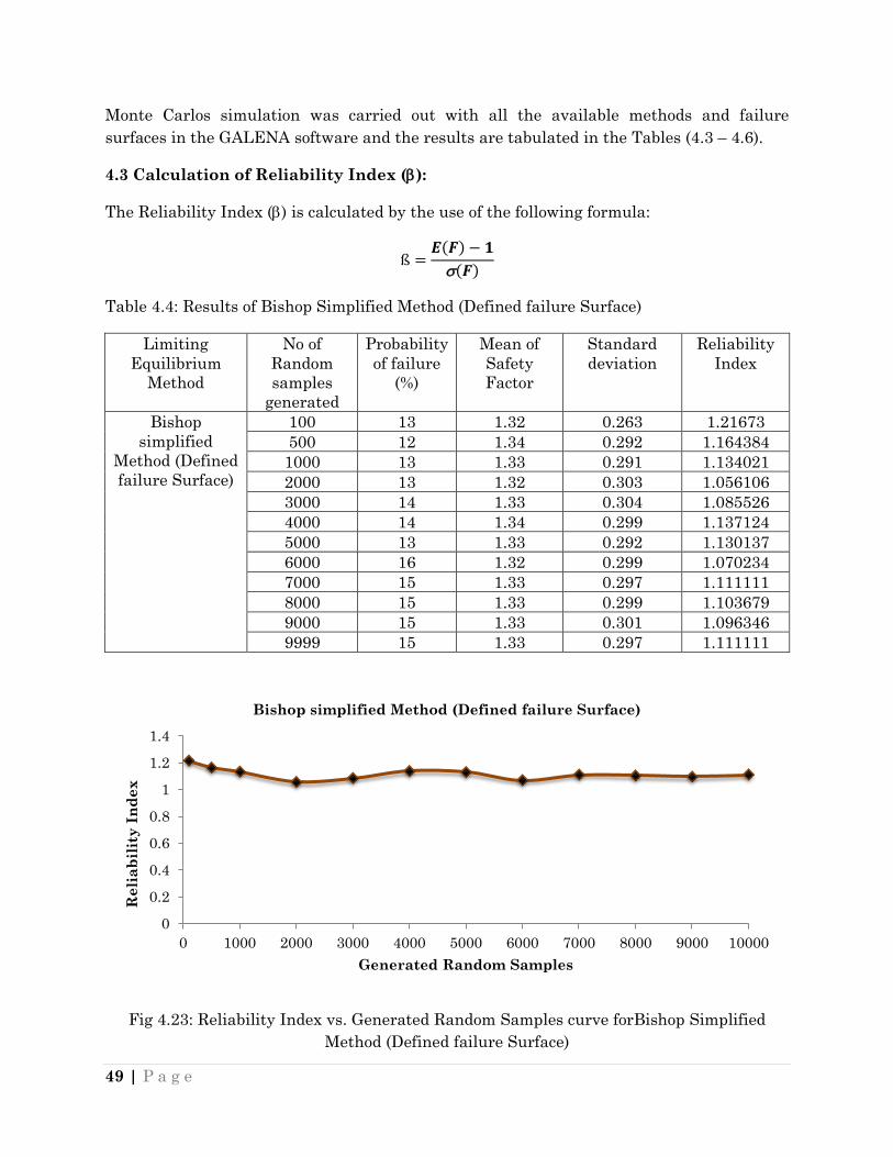
Monte Carlos simulation was carried out with all the available methods and failure
surfaces in the GALENA software and the results are tabulated in the Tables (4.3 – 4.6).
4.3 Calculation of Reliability Index ():
The Reliability Index () is calculated by the use of the following formula:
Table 4.4: Results of Bishop Simplified Method (Defined failure Surface)
Limiting
Equilibrium
Method
No of
Random
samples
generated
Probability
of failure
(%)
Mean of
Safety
Factor
Standard
deviation
Reliability
Index
Bishop
simplified
Method (Defined
failure Surface)
100 13 1.32 0.263 1.21673
500 12 1.34 0.292 1.164384
1000 13 1.33 0.291 1.134021
2000 13 1.32 0.303 1.056106
3000 14 1.33 0.304 1.085526
4000 14 1.34 0.299 1.137124
5000 13 1.33 0.292 1.130137
6000 16 1.32 0.299 1.070234
7000 15 1.33 0.297 1.111111
8000 15 1.33 0.299 1.103679
9000 15 1.33 0.301 1.096346
9999 15 1.33 0.297 1.111111
Fig 4.23: Reliability Index vs. Generated Random Samples curve forBishop Simplified
Method (Defined failure Surface)
0
0.2
0.4
0.6
0.8
1
1.2
1.4
0 1000 2000 3000 4000 5000 6000 7000 8000 9000 10000
Re
lia
bil
ity
In
dex
Generated Random Samples
Bishop simplified Method (Defined failure Surface)

50 | P a g e
Table 4.5: Results of Spencer Method (Defined failure Surface)
Limiting
Equilibrium
Method
No of
Random
samples
generated
Probability
of failure
(%)
Mean of
Safety
Factor
Standard
deviation
Reliability
Index
Spencer Method
(Defined failure
Surface)
100 8 1.36 0.272 1.323529
500 11 1.35 0.298 1.174497
1000 15 1.33 0.304 1.085526
2000 15 1.32 0.297 1.077441
3000 15 1.32 0.295 1.084746
4000 14 1.34 0.304 1.118421
5000 14 1.32 0.299 1.070234
6000 14 1.33 0.295 1.118644
7000 14 1.33 0.303 1.089109
8000 16 1.32 0.302 1.059603
9000 14 1.33 0.302 1.092715
9999 13 1.34 0.298 1.14094
Fig 4.24: Reliability Index vs. Generated Random Samples curve for Spencer Method
(Define failure Surface)
0
0.2
0.4
0.6
0.8
1
1.2
1.4
0 1000 2000 3000 4000 5000 6000 7000 8000 9000 10000
Re
lia
bil
ity
In
de
x
Generated Random Samples
Spencer Method (Defined failure Surface)
51 | P a g e
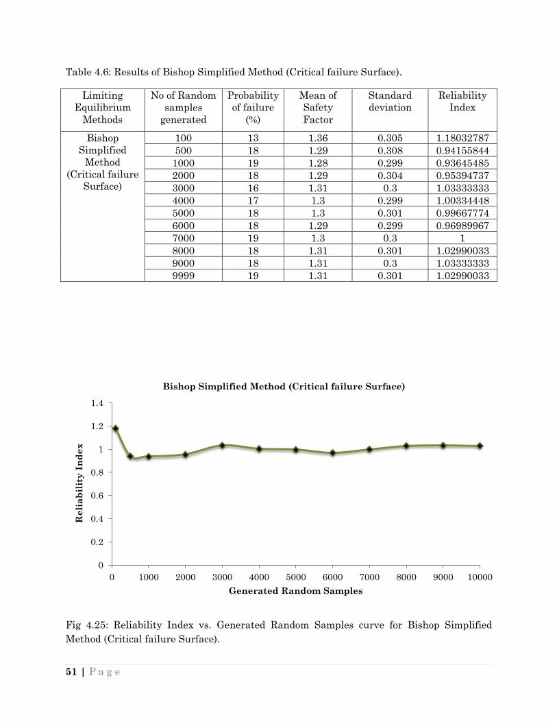
Table 4.6: Results of Bishop Simplified Method (Critical failure Surface).
Limiting
Equilibrium
Methods
No of Random
samples
generated
Probability
of failure
(%)
Mean of
Safety
Factor
Standard
deviation
Reliability
Index
Bishop
Simplified
Method
(Critical failure
Surface)
100 13 1.36 0.305 1.18032787
500 18 1.29 0.308 0.94155844
1000 19 1.28 0.299 0.93645485
2000 18 1.29 0.304 0.95394737
3000 16 1.31 0.3 1.03333333
4000 17 1.3 0.299 1.00334448
5000 18 1.3 0.301 0.99667774
6000 18 1.29 0.299 0.96989967
7000 19 1.3 0.3 1
8000 18 1.31 0.301 1.02990033
9000 18 1.31 0.3 1.03333333
9999 19 1.31 0.301 1.02990033
Fig 4.25: Reliability Index vs. Generated Random Samples curve for Bishop Simplified
Method (Critical failure Surface).
0
0.2
0.4
0.6
0.8
1
1.2
1.4
0 1000 2000 3000 4000 5000 6000 7000 8000 9000 10000
Re
lia
bil
ity
In
de
x
Generated Random Samples
Bishop Simplified Method (Critical failure Surface)
52 | P a g e
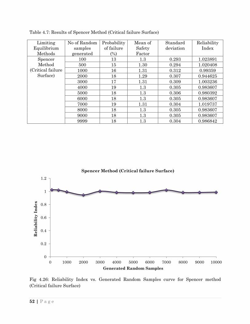
Table 4.7: Results of Spencer Method (Critical failure Surface)
Limiting
Equilibrium
Methods
No of Random
samples
generated
Probability
of failure
(%)
Mean of
Safety
Factor
Standard
deviation
Reliability
Index
Spencer
Method
(Critical failure
Surface)
100 13 1.3 0.293 1.023891
500 15 1.30 0.294 1.020408
1000 16 1.31 0.312 0.99359
2000 18 1.29 0.307 0.944625
3000 17 1.31 0.309 1.003236
4000 19 1.3 0.305 0.983607
5000 18 1.3 0.306 0.980392
6000 18 1.3 0.305 0.983607
7000 19 1.31 0.304 1.019737
8000 18 1.3 0.305 0.983607
9000 18 1.3 0.305 0.983607
9999 18 1.3 0.304 0.986842
Fig 4.26: Reliability Index vs. Generated Random Samples curve for Spencer method
(Critical failure Surface)
0
0.2
0.4
0.6
0.8
1
1.2
0 1000 2000 3000 4000 5000 6000 7000 8000 9000 10000
Re
lia
bil
ity
In
de
x
Generated Random Samples
Spencer Method (Critical failure Surface)
53 | P a g e
It is concluded from the Monte Carlo simulation that, with increase in number of iterations
the factor of safety vs. frequency curve (Fig 4.11 – 4.22) takes the shape of normal
distribution curve and the reliability index becomes more or less the same. So, it shows the
convergence of individual parameters to produce the factor of safety.
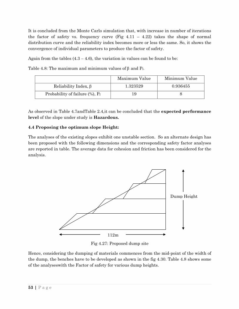
Again from the tables (4.3 – 4.6), the variation in values can be found to be:
Table 4.8: The maximum and minimum values of and Pf.
Maximum Value Minimum Value
Reliability Index, 1.323529 0.936455
Probability of failure (%), Pf 19 8
As observed in Table 4.7andTable 2.4,it can be concluded that the expected performance
level of the slope under study is Hazardous.
4.4 Proposing the optimum slope Height:
The analyses of the existing slopes exhibit one unstable section. So an alternate design has
been proposed with the following dimensions and the corresponding safety factor analyses
are reported in table. The average data for cohesion and friction has been considered for the
analysis.
Fig 4.27: Proposed dump site
Hence, considering the dumping of materials commences from the mid-point of the width of
the dump, the benches have to be developed as shown in the fig 4.30. Table 4.8 shows some
of the analyseswith the Factor of safety for various dump heights.
Dump Height
112m
54 | P a g e
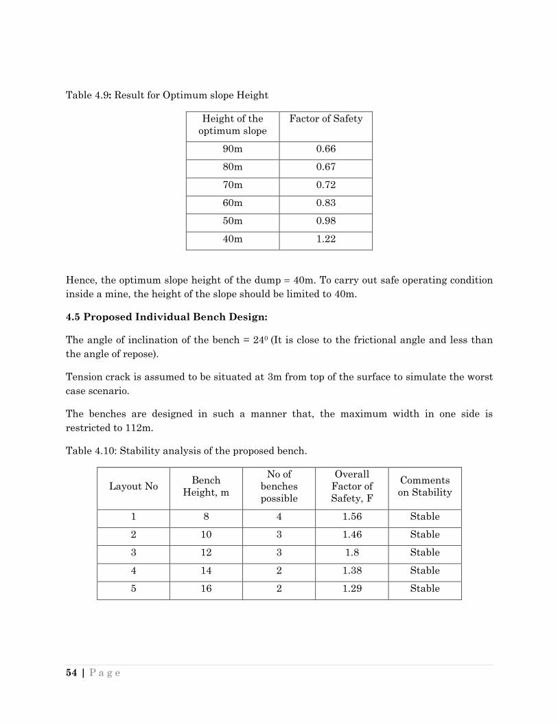
Table 4.9: Result for Optimum slope Height
Height of the
optimum slope
Factor of Safety
90m 0.66
80m 0.67
70m 0.72
60m 0.83
50m 0.98
40m 1.22
Hence, the optimum slope height of the dump 40m. To carry out safe operating condition
inside a mine, the height of the slope should be limited to 40m.
4.5 Proposed Individual Bench Design:
The angle of inclination of the bench = 240 (It is close to the frictional angle and less than
the angle of repose).
Tension crack is assumed to be situated at 3m from top of the surface to simulate the worst
case scenario.
The benches are designed in such a manner that, the maximum width in one side is
restricted to 112m.
Table 4.10: Stability analysis of the proposed bench.
Layout No Bench
Height, m
No of
benches
possible
Overall
Factor of
Safety, F
Comments
on Stability
1 8 4 1.56 Stable
2 10 3 1.46 Stable
3 12 3 1.8 Stable
4 14 2 1.38 Stable
5 16 2 1.29 Stable
55 | P a g e
CHAPTER 5
CONCLUSION AND RECOMMENDATION
5.1 Conclusion:
The following conclusions have been drawn from the investigation.
The dump contains heterogeneous materials, whose properties vary throughout the
dump.
At places large sized boulders (60cm) are dumped in these sections. While dumping,
air gap remains between them. During rainy season, the pit top water moves through
these areas. Hence, the slope becomes potentially weak.
The factor of safety for the sections AA‟, BB‟ and DD‟ are greater than 1.3, which shows
the stability of those regions. But at section CC‟, the factor of safety is found to be 0.86,
confirming that the section has already failed.
The tension crack was assumed to be situated at 3m from the slope surface. Since,
multiple restraint analysis is done; factor of safety is not affected much by the position
of the tension crack in the slope.
Though Monte Carlo Simulation concludes that the slope is in a Hazardous condition,
but field visits inferred no such results. This can be explained by the following reasons:
1) The distribution of cohesion of bench „A‟ generate some negative values, which are
not included in the simulation, thereby increasing the no of samples which fail to
produce a result.
2) The Direct Monte Carlo simulation is successful if the sample sizes are greater than
10,000, which is not possible in Galena.
3) The Bessel‟s correction was not applied despite the sample sizes for practical
purposes being less than 30.
4) Laboratory analysis of lesser number of samples.
5.2 Recommendation:
In this investigation, a few prospects of slope stability; as slope of the bench, height of
bench as well as angle of internal friction, cohesion and density of the material has been
determined. However there are many factors that affect the slope stability such as ground
water table, grain size of the dumped material, etc. So it is strongly recommended that the
following may be taken into consideration in future.
56 | P a g e
The samples were not taken to the complete depth; the samples have been taken just
from 2-3 feet depth and they do not represent the exact field conditions.
Proper provisions have to be made for the channelization of the rain water by
constructing the suitable drains surrounding the dump yard.
Segregation of the dump has to be done properly i.e. according to the size of the disposed
material. The fines should be dumped separately, and so the boulders.
In the analysis, the phreatic surface should have been included.
Though Limit equilibrium method is used for analysis, sometimes it fails to produce the
accurate result. So, Finite equilibrium method may be considered for the analysis and
evaluate its effectiveness in the analysis.
57 | P a g e
REFERENCES
1) McCarthy, David F., Essentials of Soil Mechanics and Foundations, Pearson
Prentice Hall publication, pp 657-718, (2007).
2) Murthy, V.N.S., Principles of Soil Mechanics and Foundation Engineering, Fifth
Edition, UBS Publisher‟s Ltd, (2001).
3) Husein Malkawi A.I., Hassan W.F., Abdulla F., Uncertainty and reliability analysis
applied to slope stability. Structural Safety Journal; 22:161–87, (2000).
4) US Army Corps of Engineers, Engineering and Design - Slope Stability, Washington
DC, USA: US Army Corps of Engineers, (2003).
5) Flora C.S., Evaluation of Slope Stability for Waste Rock Dumps in a Mine,
(http://www.ethesis.nitrkl.ac.in/1386/1/Thesis_2.pdf), (2008).
6) Husein Malkawi A.I., Nusairat J.H., Alkasawneh W., Albataineh N., A comparative
study of various commercially available programs in slope stability analysis.
Computers and Geotechnics 35; 428-435 (2008).
7) Li L.C., Tang C.A., Zhu W.C., Liang Z., Numerical Analysis of slope stability using
gravity increase method. Computers and Geotechnics 36; 1246–1258(2009).
8) Radhi M.S., Pauzi N.I., Omar H., Probabilistic of rock slope stability Analysis using
Monte Carlo Simulation. International Conference on Construction and Building
Technology International (2008)
9) Priest S.D., Brown E.T., Probabilistic stability analysis of variable rock slopes,
Trans. Min. Sci. & Metallurgy, Sect A; 92, pp 1-12 (1983).
10) Wang Y., Cao Z., and Au S., Practical reliability analysis of slope stability by
advanced Monte Carlo simulations in a spreadsheet. Can. Geotech. J.; 162-172 2011.
11) Steiakakis E., Kavouridis K., Monopolis D., Large scale failure of the external waste
dump at the “South Field” lignite mine, Northern Greece, Engineering Geology 104;
269–279, (2009).
12) US Army Corps of Engineers, Reliability Analysis and Risk Assessment for Seepage
and Slope Stability Failure Modes for Embankment Dams, Washington DC, USA:
US Army Corps of Engineers, (2006).
13) Lacasse, S. and Nadim, F., Uncertainties in Characterizing Soil Properties,
Proceedings, Uncertainty in the Geologic Environment: from Theory to Practice,
Geotechnical Special Publication No. 58, ASCE, Vol. 1, pp. 49-75 (1996).

58 | P a g e
14) “Factor of safety and probability of failure” – Retrieved from
www.rocscience.com/.../8_Factor_of_safety_and_probability_of_failure.pdf
15) ASTM Standard D2850,Standard Test Method for Unconsolidated-Undrained
Triaxial Compression Test on Cohesive Soils, ASTM International, West
Conshohocken, PA, (2007).
16) ASTM Standard D698, Standard Test Methods for Laboratory Compaction
Characteristics of Soil Using Standard Effort, ASTM International, West
Conshohocken, PA, (2007).
17) GALENA User‟s Guide, version 5.0, Clover Technology, Australia.
18) R User‟s Guide, version 2.12.2