analysis of strapdown sensor testing - ntrs.nasa.gov · the analytic sciences corporation table of...
TRANSCRIPT

TR-147-2
ANALYSIS OF
STRAPDOWN SENSOR TESTING
Final Report
June 30, 1970
https://ntrs.nasa.gov/search.jsp?R=19730010914 2019-09-09T11:52:46+00:00Z

THE ANALYTIC SCIENCES CORPORATION
TR-147-2
ANALYSIS OF
STRAPDOWN SENSOR TESTING
Phase H Final Report
June 30, 1970
Prepared Under:
Contract Number NAS12-678
for
NATIONAL AERONAUTICS AND SPACE ADMINISTRATIONElectronics Research CenterCambridge, Massachusetts
Prepared by:
Bard S. Crawford
Approved by:
Arthur A. Sutherland, Jr.Arthur Gelb
THE ANALYTIC SCIENCES CORPORATION6 Jacob Way
Reading, Massachusetts 01867

THE ANALYTIC SCIENCES CORPORATION
Mr. Edward Spitzerand
Mr. Maurice LanmanTechnical Monitors
NAS 12-678Electronics Research Center
575 Technology SquareCambridge, Massachusetts 02139
iii

THE ANALYTIC SCIENCES CORPORATION
FOREWORD
This document describes the results of astudy begun in 1968 for the NASA Electronics Re-search Center. The underlying objective was tohelp in choosing laboratory test equipment and pro-cedures, especially in the light of the increasinginterest in strapdown technology,, This report is anexpanded version of Reference 10. New materialincludes analysis of tests performed on pulse re-balanced sensors, a new treatment of input-dependentoscillations in ternary and binary pulse rebalanceloops (Appendix F) and some illustrative nomographsrelating desired test accuracy to required testequipment performance.
'V

THE ANALYTIC SCIENCES CORPORATION
ABSTRACT
Some topics related to dynamic testing ofstrapdown sensors are analyzed, with emphasis onmeasuring parameters which give rise to motion-induced error torques in single-degree-of-freedominertial sensors. The objective is to determine thedynamic inputs, test equipment characteristics anddata processing procedures best suited for measuringthese parameterso Single-axis, low frequency vi-bration tests and constant rate tests are studied indetail. Methods for analyzing the effects of testmotion errors and measurement errors are develop-ed and illustrated by examples. They are shown tobe useful in predicting achievable test accuraciesand required test times. Candidate test data proc-essing methods are compared and recommendationsconcerning test equipment and data processing aremade.
Vll
THE ANALYTIC SCIENCES CORPORATION
TABLE OF CONTENTS
PageNo.
FOREWORD v
ABSTRACT • vii
List of Tables xii
List of Figures xv
1. INTRODUCTION 1
lol Objectives of Study 21.2 Organization of the Report 7
2. ERROR MODELS AND BASIC PARAMETER GROUPS 11£
2.1 Single-Degree-of-Freedom Inertial Sensors 112.2 Test Objectives 152.3 Motion-Induced Error Torques 20
2.3» 1 Single-Degree-of-Freedom Gyros:Angular Motion 22
2.3.2 Single-Degree-of-Freedom Gyros:Linear Motion 23
2.3.3 Single-Degree-of-FreedomAccelerometers: Angular Motion 24
2.3.4 Single-Degree-of-FreedomAccelerometers: Linear Motion 25
2.4 Basic Parameter Groups 262.4.1 Analog Rebalancing 262.4.2 Pulse-Rebalancing 34
2.5 Test Motion Possibilities 36
3. SINGLE-AXIS, LOW-FREQUENCY TESTING 41
3.1 Observable Quantities 413.1.1 Vibration Testing 423.1.2 Constant Angular Rate Testing 513.1.3 Summary:Angular Motion Test
Observables 52
IX

THE ANALYTIC SCIENCES CORPORATION
TABLE OF CONTENTS (Continued)
3.2 Single-Axis Test Accuracy 553.2.1 Overview and Comparison 553.2.2 Bias Test Motion Errors 653.2.3 Cyclic Test Motion Errors 703.2.4 Errors Due to Quantization 793.2.5 Errors Due to Pulse Rebalancing 853.2.6 Random High Frequency Errors 1003.2.7 Rebalance Loop Errors 1053.2.8 Errors Due to Parameter Changes 113
3.3 Test Duration 1153.3.1 Choice of Sample Interval 1173.3.2 Effects of Quantization: Examples 1183.3.3 Time to Reach Equilibrium 126
3.4 Test Data Processing 1293.4.1 Fourier Analysis 1303.4.2 Least Squares Estimation 1353.4.3 Kalman Filtering 137
3.5 Example Calculations 1403.5o 1 Torque Levels 1403.5»2 Test Errors 144
4. IMPLICATIONS FOR TEST LABORATORYEQUIPMENT 163
4.1 Test Motion Machinery 1634.2 Data Processing Equipment 171
5. CONCLUSION 175
5.1 Summary of Findings 1755.2 Recommendations 177

THE ANALYTIC SCIENCES CORPORATION
TABLE OF CONTENTS (Continued)
PageNo.
APPENDICES
Appendix A
Appendix B
Appendix C
Appendix D
Appendix E
Appendix F
REFERENCES
Derivation of Trigonometric SeriesCoefficients: Vibration Testing of Single-Degree-of-Freedom Sensors
Test Motion Bias Error Analysis:Angular Vibration Testing of Single-Degree-of-Freedom Gyro
Kalman Filtering Formulation
Fourier Analysis Equations for PulseRebalanced Testing
Survey of Strapdown Sensor TestMethods, 1968
Analysis of Oscillations in Ternary andand Binary Rebalance Loops
181
187
201
223
233
237
267
XI

THE ANALYTIC SCIENCES CORPORATION
LIST OF TABLES
Table PageNo, No.
2,3-1 Gyro Notation 212.3-2 Accelerometer Notation 21
2.4-1 Basic Parameter Groups 28
3.1-1 Fourier Coefficients: Gyro Angular Vibration Tests 46
3.1-2 Fourier Coefficients: Accelerometer AngularVibration Tests 47
3.1-3 Fourier Coefficients: Gyro and AccelerometerLinear Vibration Tests 50
3.1-4 Applied Torque Expressions: Constant Rate Testing 523.1-5 Determinable Gyro Parameter Groups: Angular
Motion Testing 53
3.2-1 Test Error Influences 56
3.2-2 Error Analysis Summary 603.2-3 Summary Comparison of Single-Axis Test Methods 633.2-4 Normalized Error Coefficients: Bias Test Motion 69
Errors 69
3.2-5 Significant Cyclic Errors 713.2-6 Characteristic Frequency and Amplitude and Test
Measurement Error in Pulse Rebalance Loops 953.2r7 Nonlinearity Effects on Sinusoid 109
3.3-1 Example Errors Due to Quantization: AnalogRebalancing 120
3.3-2 Example Errors Due to Quantization: PulseRebalancing 125
Xlll

THE ANALYTIC SCIENCES CORPORATION
LIST OF TABLES (Continued)
Assumed Gyro Parameter Values 141Illustrative Torque Levels 142Assumed Error Source Values 147
Example Error Summary: o Test Axis 148Example Error Summary: s Test Axis 149Example Error Summary: i Test Axis 150
Example Error Summary: o/s Test Axis 151Example Error Summary: i/o Test Axis 152Example Error Summary: i/s Test Axis 153Example Errors: Summary Comparison 155
B-l Specialization to Six Cases of Interest 197
xiv

THE ANALYTIC SCIENCES CORPORATION
FigureNo.
1.1-1
1.1-2
1.1-3
2.1-1
2.1-2
2.1-3
2.2-1
3.1-1
3.1-2
3.1-3
3.2-1
3.2-2
3.2-3
3.2-4
3.2-5
3.2-6
3.2-7
3.2-8
3.2-9
3.2-10
LIST OF FIGURES
Test Sequence Flow Diagram
Dynamic Testing and Data Processing
The Strapdown Sensor Test Problem
Single Degree of Freedom GyroSingle Degree of Freedom Pendulous Accelerometer
Rebalance Loop Configurations
General Test of a Single-Degree-of-FreedomSensor
General Single-Axis Angular Vibration Test
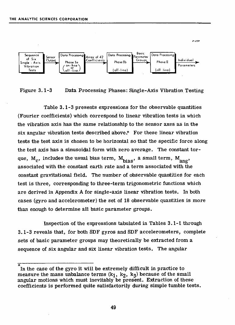
Six Candidate Test OrientationsData Processing Phases: Single-Axis VibrationTesting
Distorted Test Motion Sinusoids
Euler Angles Relating Base Axes to Table Axes
Pulse SequenceDistribution of Error Due to Quantization
Block Diagram of a Generalized Rebalanced Loop
RMS Change in a' with a Fixed Phase Difference
Frequency of Oscillation versus Input Level forTernary and Binary Rebalance Loops
Final Accuracy and Test Time: Random Errors
Torquer Nonlinearities
Linear Sensor Loop with Disturbance FunctionAdded
PageNo.
4
5
6
12
15
16
17
44
45
49
72
75
80
80
88
92
96
104
107
110
XV

THE ANALYTIC SCIENCES CORPORATION
FigureNo.
3.3-1
3.3-2
3.3-3
3.5-1
3.5-2
4.1-1
4.1-2
4.1-3
B-l
C-l
C-2
D-l
F.l-1
F.l-2
F.l-3
F.I -4
Fol-5
F.I -6
F.l-7
F.2-1
LIST OF FIGURES (Continued)
Time -Dependent Test ErrorsEffective Drift Rate Due to QuantizationEstimation Error Variance Time History
Variation of Torque Levels with Test MotionAmplitude and Frequency: o and s Test AxesVariation of Torque Levels with Test MotionAmplitude and Frequency: i, o/s, i/o andi/s Test Axes
Nomograph for Distortion Effect - SmallSignal CasesNomograph for Quantization Effect - ConstantRate TestingNomograph for Quantization Effect - SinusoidalAveraging
Test Axis Misalignment Angles
Numerical Integration ResultsImprovement in Small Term Estimate Due toCorrelation
Binary Pulse Rebalancing Waveforms
Ternary Rebalance LoopFloat Angle Time History SegmentsExample Periodic Time HistoriesSolution for Normalized PeriodNormalized Period Versus Normalized InputNormalized Amplitude Versus Normalized InputSummary of Results - Ternary LoopSummary of Results - Binary Loop
PageNo.
117
122
127
145
146
166
166
167
192
216
217
224
239
239
245
252
256
261
262
265
XVI

THE ANALYTIC SCIENCES CORPORATION
1, INTRODUCTION
The potential advantages of strapdown or gimballess inertialsystems over conventional, gimballed systems have been recognized forsome time (Ref. 1). These include flexible packaging, low power con-sumption, weight and volume, easy assembly and maintenance and con-venient use of navigation sensors in autopilot functions. Continuingadvances in the development of smaller, faster and more compact digitalcomputers have led to increased interest in strapdown systems. It isclear that these devices will perform acceptably for certain missions andwill be, in some cases, superior in overall cost and reliability.
With the advent of strapdown inertial systems, new problems inachieving high sensor accuracies have arisen. Platform systems isolatethe inertial sensors from most rotational motion. However, when theinstruments are rigidly attached to the vehicle, they can be subjected toa severe angular motion environment, resulting in errors which can berectified both in the instrument and in the attitude transformation calcu-lation. For example, Ref. 2 shows that the magnitudes of vibration-induced errors can be considerably greater than gyro drift rates which areusually acceptable for navigation applications. Errors of this kind are notobserved during static tests. Thus, in order to measure their effectsaccurately enough to assure adequate compensation during operation,strapdown sensors must be subjected to dynamic testing.
Torque rebalance loops, which are a common feature of strap-down sensors, lead to additional errors, as well as creating problems intesting for motion-induced disturbance torques. While they provide datain a form suitable for digital navigation computers, pulse rebalance loops

THE ANALYTIC SCIENCES CORPORATION
in particular introduce essential nonlinearities which complicate thedynamic testing problem.
1.1 OBJECTIVES OF STUDY
The objectives of this study are summarized briefly as follows:
• Determine the input dynamical forcing functions bestsuited for testing for all significant error coefficients.
• Determine necessary test durations and the nature andaccuracies required of the essential test equipment.
• Compare alternative methods of test data processing,considering the possibilities for both on-line andoff-line computation.
• Suggest alternative test procedures which may substitutesophisticated test data processing for complex testmotion machinery.
• Devise test procedures which will establish an under-standing of statistical predictability in the stability ofsensor parameters.
Substantial progress has been made regarding the first fourobjectives in the above list.
The investigation concerns testing for certain parameters whichcause errors in single-degree-of-freedom sensors, especially those fac-tors associated with angular motion, and therefore uniquely important forstrapdown sensors. These parameters correspond to a set of fixedmechanical properties, such as products of inertia of various elementsof an instrument and the alignment of sensor components with respect to

THE ANALYTIC SCIENCES CORPORATION
one another. Rebalance loop errors such as fixed scale factor error andtorquer nonlinearity are also considered. The study has not been con-cerned with such items as torquer scale factor changes, friction, thermalgradients and electromagnetic effects, all of which may combine withangular motion to cause errors. Problems associated with rebalance loopdynamics are not treated (except in the treatment of test errors due topulse rebalancing), but will be the subject of future work related to highfrequency testing.
The ultimate goal of this effort is to help formulate completetest sequences, such as that pictured in Fig. 1.1-1. The illustratedsequence begins with a set of physical measurements on the basic sensorcomponents, moves to a set of conventional static and low-rate tests whichproduce estimates of the quantities normally sought for platform appli-cations, and concludes with a set of dynamic tests designed to extract theparameters uniquely important in strapdown applications. The require-ments of a particular test sequence depend of course on the underlyingreasons for the test. Are they, for example, related to a research pro-gram aimed at developing new sensors, or are they part of a mission-oriented program involving a series of qualification and calibration tests?The development presented herein is general enough to cover bothsituations.
The report describes an analysis of dynamic testing of single-degree-of-freedom sensors, emphasizing single-axis testing. This typeof testing involves the hardware elements pictured in Fig. 1.1-2, con-nected together as indicated. The sensor outputs and test table outputsfeed data into a computer, either directly for real-time processing, orby way of a data storage medium for subsequent processing. Elementsof the strapdown sensor test problem are illustrated in Fig. 1.1-3. Themain test objectives are to determine the magnitude and stability of

THE ANALYTIC SCIENCES CORPORATION
PHYSICAL MEASUREMENTS
on Sensor Components
K-821
dimensions, mass, inertia, etc.
STATIC AND LOW RATE TESTING
for example:
Torque-to-Balance Tests
Servoed - Table
DYNAMIC TESTING
for example;High Constant Rate TestsAngular Vibration TestsLinear Vibration Tests
DATA PROCESSING
Hand CalculationsComputer
mass unbalance
random drift
scale factor etc.
DATA PROCESSING
motion - inducederror coefficients
Figure 1.1-1 Test Sequence Flow Diagram

THE ANALYTIC SCIENCES CORPORATION
R -820
Figure 1.1-2 Dynamic Testing and Data Processing

THE ANALYTIC SCIENCES CORPORATION
PRESCRIBED TEST MOTION
TEMOiERR
"
TEST |JEQUIPMENT 1 "
ST''IONORS
•\ MOTIONSJ T *
1
1
1 TES_ MOT
"*" SEN(OPTIC
SENSOROUTPUTERRORS
STRAPDOWN I X
SENSOR \SENSOR 'U
TION fc-^V50RS VN A L ) A
MOTIONSENSORERRORS
\ i
DATA 1 PARAMETERPROCESSING 1 ^"ESTIMATES
]
J
*
DETERMINE :• ALL PARAMETERS WHICH CAUSE ERROR TORQUE
• STABILITY OF PARAMETERS
Figure 1.1-3 The Strapdown Sensor Test Problem
parameters which cause error torques. Test errors are associated withimperfections in the motion-supply ing equipment, the (optional) sensorswhich may be used to measure the applied motion and those parts of thestrapdown sensor itself which are used as a measuring instrument (suchas torque rebalance electronics). The immediate goal of the study is torecommend input motions and data processing procedures and.to analyzethe effects of test errors on overall test accuracy and duration.

\
THE ANALYTIC SCIENCES CORPORATION
1.2 ORGANIZATION OF THE REPORT
In Chapter 2 the overall test objective is defined as the iden-tification and measurement of the causes of sensor errors. These aregrouped into three categories: motion-induced errors (such as thosecaused by angular motion about the spin and/or output axes of a gyro),residual errors (such as those caused by thermal and friction effects)and rebalance-loop errors. Models for certain important motion-inducederrors in single-degree-of-freedom (SDF) gyros and accelerometers arepresented, and specialized in a way which is valid for testing SDF sen-sors in the closed-loop (rebalanced) configuration, using low-frequencytest motion inputs. (In this context "low frequency" means considerablyless than l/rf, where r. is the time constant associated with the sensorfloat dynamics. For typical inertial sensors a low frequency is therefore20 Hz or less.) This development leads to a two-stage testing concept:A set of basic parameter groups is measured directly from a sequence ofapplied test motions, and individual parameters are subsequently deter-mined, algebraically, from the values of the basic parameter groups.Chapter 2 concludes with a general discussion of possible test motions andintroduces some of the reasoning behind the decision to emphasize
single-axis testing.
In Chapter 3 single-axis, low-frequency testing is studied indetail. A particular sequence of sensor orientations with respect to thetest motion axis is recommended. The observable quantities from eachvibration test are a set of Fourier coefficients which define a periodicfunction representing the applied torque. A set of six angular vibrationtests and a set of six linear vibration tests provide an array of observablequantities which theoretically permit determination of a complete set ofbasic parameter groups. The observable quantities generated by constant
THE ANALYTIC SCIENCES CORPORATION
rate tests and vibration tests, in which only the average torque is mea-
sured, are also presented. Three classes of test error sources are con-sidered: test motion errors, measurement errors and changes in thesensor parameters. Motion errors and measurement errors have bias,cyclic and high-frequency noise components. Measurement errors alsoinclude the effects of quantization. Methods for analyzing all of theseerror sources are developed. The first phase of the data processingproblem, that of estimating the Fourier coefficients, is formulated as aproblem in linear estimation, for which the Kalman filter is an optimalsolution. This formulation is useful in studying the combined effect ofrandom high frequency fluctuations in test motion errors and measure-ment errors and in determining the useful test duration. The analysis ofquantization effects also lends insight into the problems of choosing testtime and the number of data samples per cycle of test motion. Threecandidates for this data processing function — Fourier analysis, leastsquares estimation and Kalman filtering -- are compared. Chapter 3concludes by summarizing the results of example calculations for asequence of constant rate and vibration tests on a SDF gyro. Illustrativevalues for the observable quantities as well as test error effects are
included.
Tentative conclusions and recommendations concerning thechoice of laboratory equipment are summarized in Chapter 4. Someillustrative nomographs relating desired test accuracy to required testequipment performance are included. Overall conclusions and a discussionofthe re commended continuation of effortare presented in Chapter 5. A signi-
ficant recommendation stemming from the study to date is that great stressshould be placed on the appropriate use of conventional single-axis testdevices, in a combined program of vibration testing and constant rate
8
THE ANALYTIC SCIENCES CORPORATION
testing of strapdown inertial sensors. In order to obtain the maximumusefulness from the test data, careful attention should be given to themeans for controlling and/or measuring the supplied motion and to tech-niques for recording and/or processing the sensor output data producedduring the tests. These points are explored in the body of the report.
Appendices A through D and F contain detailed technicalmaterial in support of the discussions contained in the main body of thereport. Appendix E summarizes a brief survey of contemporary strap-down sensor testing and test equipment.

THE ANALYTIC SCIENCES CORPORATION
2. ERROR MODELS AND BASIC PARAMETER GROUPS
This chapter provides a general discussion of single-degree -of-freedom (SDF) sensors and sensor test objectives and develops a setof equations for motion-induced error torques. Based on these relationsa set of basic parameter groups is defined. These groups in turn helpclarify the problem of selecting appropriate linear and angular motionsto be applied during tests. The possibilities for test motions areexamined at the end of the chapter.
2,1 SINGLE-DEGREE-OF-FREEDOM INERTIAL SENSORS
Gyroscopes are angular motion sensors. They are commonlybased on the use of a spinning member, the rotor, as the sensing element. *All gyroscopes which use a spinning rotor can be classified under two majorgroups: single-degree-of-freedom gyros and two-degree-of-freedom gyros.The two-degree-of-freedom gyro senses angular motion directly, bymeasuring the displacement of the rotor spin axis relative to the case.The rotor may be mounted in mechanical gimbals, or may be supportedby electric or magnetic fields as in the electrostatically suspendedvacuum gyro and cryogenic gyro.
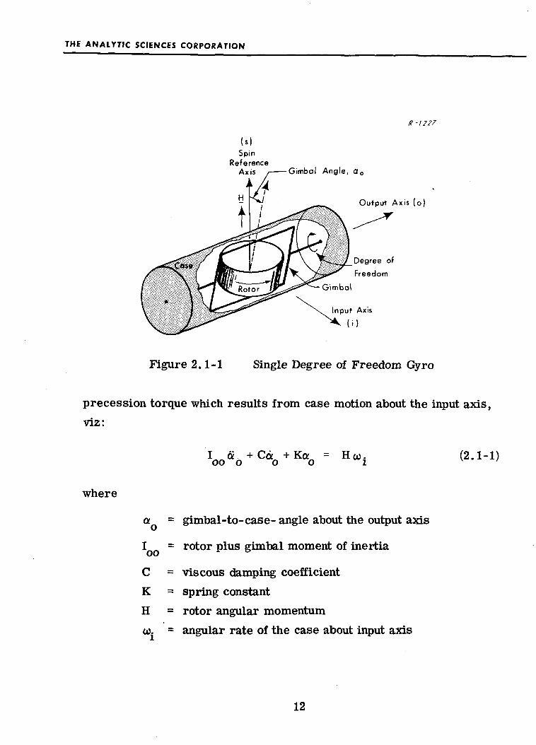
In the case of the single-degree-of-freedom (SDF) gyro thespinning rotor is mounted in a gimbal which allows only one degree-of-freedom relative to the case (see Fig. 2.1-1). The equation of motionof an ideal single-degree-of-freedom gyro can be determined by equatingreaction torques about the output axis to the "applied" gyroscopic
*Notable exceptions are the laser gyro and tuning fork gyro.
11
THE ANALYTIC SCIENCES CORPORATION
R-1227
Gimbal Angle, a0
Output Ax is (o)
Degree of
Freedom
Figure 2.1-1 Single Degree of Freedom Gyro
precession torque which results from case motion about the input axis,viz:
where
(2.1-1)
Xoo
C
K
H
gimbal-to-case- angle about the output axis
rotor plus gimbal moment of inertia
= viscous damping coefficient= spring constant= rotor angular momentum= angular rate of the case about input axis
12

THE ANALYTIC SCIENCES CORPORATION
As indicated by Eq. (2.1-1), a constant value of to. results in the followingsteady-state value of a :
Ha = K co.o is. i
Hence, this gyro is referred to as a rate gyro, as the gimbal angle is adirect measure of case rate. In the situation where K = 0, we get asteady-state gimbal angle rate,
. _ HOf- - 7T CO.o C i
Thus, gimbal angle is related directly to the integral of the input rate,and this gyro is therefore called a rate integrating gyro. By mountingthe gyro rotor in an enclosure which serves as the gimbal and floatingthe whole assembly in a fluid of appropriate density, the gyro output axisbearings are unloaded, reducing some unwanted torques. This con-figuration, called the floated rate integrating gyro, is extensively usedfor very high accuracy applications such as inertial navigation.
In gimballed platform applications, the gyro float angle, a , iscontinuously nulled by platform gimbal servo action. In strapdown systemapplications, the gyro float angle is nulled by the application of a torquegenerated by passing an electric current through the windings of an outputaxis torquer. The current, which may be continuous (analog) or a seriesof pulses (digital), is derived from a measurement of the float angle. Theclosed loop comprised of float dynamics, float angle pick-off, torquing
electronics and output axis torquer is called the rebalance loop. The
rebalance current is taken as a measure of input rate (for continuous
13

THE ANALYTIC SCIENCES CORPORATION
torqued gyros) or incremental input angle (for pulse torqued gyros).Figure 2. 1-3 shows a general schematic diagram of a strapdown gyro
rebalance loop, including the following three types of torquing electronics:linear analog- rebalancing, binary pulse-rebalancing and ternary pulse-rebalancing.
The single-degree-of-freedom pendulous accelerometer isillustrated in Fig. 2.1-2. Two major differences between this repre-sentation of the instrument and that presented for the SDF gyro areobvious. The direction perpendicular to the output and input axes iscalled the pendulum (p) axis rather than the spin(s) axis. Also, the
instrument is assumed to consist of only two basic parts: a case and acombination gimbal and pendulum. The equation of motion of an "ideal"single-degree-of-freedom accelerometer is:
roo % + Cdo + *•„ = -m 6P
where the quantities not previously defined are :
m = gimbal plus pendulum mass6 = displacement of the center of massf. = specific force on the case, along
the input axis
Strapdown accelerometers use the same kinds of rebalancetorquing schemes as those illustrated above for strapdown gyros. Therebalance current in this case is a measure of input specific force (forcontinuous torqued accelerometers) or incremental changes in the integralof the input specific force (for pulse torqued accelerometers).
14

THE ANALYTIC SCIENCES CORPORATION
K -1228
(p)
PendulumReference
AxisGimbal Angle,ao
Output Ax is ( o )
Degree ofFreedom
Figure 2.1-2 Single Degree of Freedom Pendulous Accelerometer
2.2 TEST OBJECTIVES
A block diagram representation of a general test of a SDFfloated sensor in the torque-rebalancing configuration is shown inFig. 2.2-1. The diagram illustrates the sensor's nature as a devicewhich sums torques acting on the floated member. The "applied" torque,M , consisting of the input (gyroscopic or pendulous) torque and dis-aturbance torque, M ,, is opposed by the torque-generator torque, M. .The latter is fed back through the rebalance loop, in a manner whichtends to null the net torque about the gimbal output axis, M .
The controlled test environment includes all quantities (motion,orientation, temperature, etc,) which cause input torques or disturbance
torques to be applied. By carefully controlling and/or measuring these
15

THE ANALYTIC SCIENCES CORPORATION
R-1278
FloatDynamics
SignalGenerator
Scaled^•Indicated
Rate
A
PoisesIndicatingingle Change
PulsesIndicating
Angle Change
Figure 2.1-3 Rebalance Loop Configurations
16

THE ANALYTIC SCIENCES CORPORATION
TestControls
H
DynTe
Enviro
MEASUREMENTS OF ENVIRONMENT ^ |
amicstnment Md jr"^i.
M,9
= Gyro Rotor Angular Momentum
Processor 1 Results
y ' 'SensorMeasurements
M fen Analog-\ • Float 1 ° Signal ea °r. e-
J Dynamics 1 Generator » i i u• Rebalance
Torque 1 '|9
Generator 1
mSp = Accelerometer Pendulosity
Figure 2.2-1 General Test of a Single-Degree-of-Freedom Sensor
quantities the test operator seeks to isolate and calibrate various sourcesof disturbance torque. From the gyro itself the only quantities availableas inputs to the data processor are the voltages, e and er. The signal-generator output, e , is a voltage which is proportional to the float anglea . The output, e , of the block labeled "rebalance electronics" is ananalog or digital indication of the rebalance torque M. . In the analog-rebalance case the function of the rebalance electronics is to generate acontinuous current, i. , which is proportional to the voltage, e . In thiscase there is only one available output (ea = er) which is a measure ofboth the float angle time history and the rebalance torque. In the pulse-rebalance case e is the sampled output of a nonlinear element; it is usedto determine the sign of a fixed-magnitude torque applied to the sensor.
The overall test objective can be defined as the identificationand measurement of the causes of sensor errors; that is, all causes fora discrepancy between the output of the sensor and the quantity which that
17

THE ANALYTIC SCIENCES CORPORATION
output is supposed to represent. The output of a strapdown gyro is either
a continuous indication of the input-axis angular rate, co., or a digitalindication of incremental changes in the integral of w.. Similarly, theoutput of an accelerometer is a continuous or digital indication of theinput-axis specific force, f., or incremental changes in the integral of f..
Sensor error sources may be grouped as follows:
• Motion-Induced Error Torques
Error torques are the various components of thedisturbance torque, M^, shown in Fig. 2.2-1.Motion-induced error torques are those directlyassociated with case motions, either angular orlinear. They are sometimes referred to as"dynamic errors."
• Residual Error Torques
Residual error torques are all components of M^ notassociated with case motions. For example:
Torques due to temperature gradients or non-standard temperatures.
Torques associated with the orientation of thesensor. These could include mass unbalanceeffects during an angular motion test. (Thesame parameters lead to motion-inducedtorques during a linear vibration test).
Undesired friction torques
Undesired elastic restraint torques
Undesired electromagnetic effects
Torques of unknown origin
Any of these may of course change with time. How-ever, during the relatively short test durationsrequired for the dynamic tests proposed the abovetorques are expected to exhibit very little variation.
18

THE ANALYTIC SCIENCES CORPORATION
• Rebalance-Loop Errors
Two broad types of rebalance-loop errors exist,as follows:
The causes of discrepancies between therebalance torque and the value indicated by thesensor output. Examples are torquer scale-factor error and torquer nonlinearity.
Errors associated with sensor loop dynamicswhich are not fast enough to follow the inputmotion. In such a case the rebalance torquetime history is not a perfect replica of theapplied torque time history.
The main emphasis in this report is on testing formotion-induced errors, with some attention paid to torquer errors.Residual errors are not treated, except in the recognition that a "bias"error torque is always present during a test involving applied motions.Errors associated with the dynamics of the rebalance loop are not treated,but will be the subject of future work related to high-frequency testing.
One approach to testing for motion-induced errors is to assumeno prior knowledge of the physical causes of such errors and to design aprocedure which seeks to discover the functional relationship betweenM, and various motions. Another approach is to start with a physically-derived error model which defines such a functional relationship in termsof unspecified parameters, and to design a testing procedure which seeksto determine those parameters. The latter method is followed below.However, if all the effects in the first technique are accounted for by oneor more parameters in the second approach, the two are equivalent andthe kind of testing described in Chapter 3 has considerable merit in either
case. (This point is discussed further in Section 2.4.)
19

THE ANALYTIC SCIENCES CORPORATION
2.3 MOTION-INDUCED ERROR TORQUES
This section presents a set of physically-derived error
models for motion-induced error torques in SDF gyros and accelerom-
eters. These error models are taken from equations derived in Refs. 2
and 3. A general expression for the total "applied" output-axis
torque is:
M = M. . +M + M.. (2.3-1)a Tnas ane; lin v '
where
M.. = a random bias error torque nots associated with motion
M = the torque induced by angularansr , . j < ^ >& motions
M.. = the torque induced by linearn motions
The error models presented below are given as expressions for M and
M.. for the two types of sensors. The notation used is summarized
in Tables 2=3-1 and 2.3-2. For any particular test situation the
total applied torque as given in Eq<,(2.3-l) must be considered.
20

THE ANALYTIC SCIENCES CORPORATION
TABLE 2.3-1
GYRO NOTATION
f , f . , f g = case linear specific force
iii. u., u, = case angular ratesO 1 S
(i ,u>.,u; = case angular accelerations
a ,a.,a = gimbal-to-case angular misalignments
8 , (I. = rotor-to-gimbal angular misalignments
I ,!..,! = float moments of inertia (includinggimbal and rotor components)
Ioor'Iiir'
Issr= rotor moments of inertia
= gimbal products of inertia
O = rotor spin rate relative to the gimbal8
H = !.„ 0_
, 6 = float center of mass displacements
m = float mass
K..,K = direct compliances11 SS
K. ,K .,K ,K. = cross compliances
The subscripts, o, i, s refer to output, input and spinaxes, respectively.
TABLE 2.3-2
ACCELEROMETER NOTATION
w0, ov
I .I...Ioo H pp
V6i
K...Ku ssK.. , K .. K , K.
ip pi po 10
= case linear specific force resolvedinto case-fixed axes
= case angular rates resolved intocase-fixed axes
= gimbal-to-case angular misalignments
= float moments of inertia
= float products of inertia
= float center of mass displacements(in the absence of acceleration)
= float mass
= direct compliances
= cross compliances
The subscripts o, i, p refer to output, Input and pendulumaxes, respectively.
21
THE ANALYTIC SCIENCES CORPORATION
2,3.1 Single-Degree-of-Freedom Gyros: Angular Motion
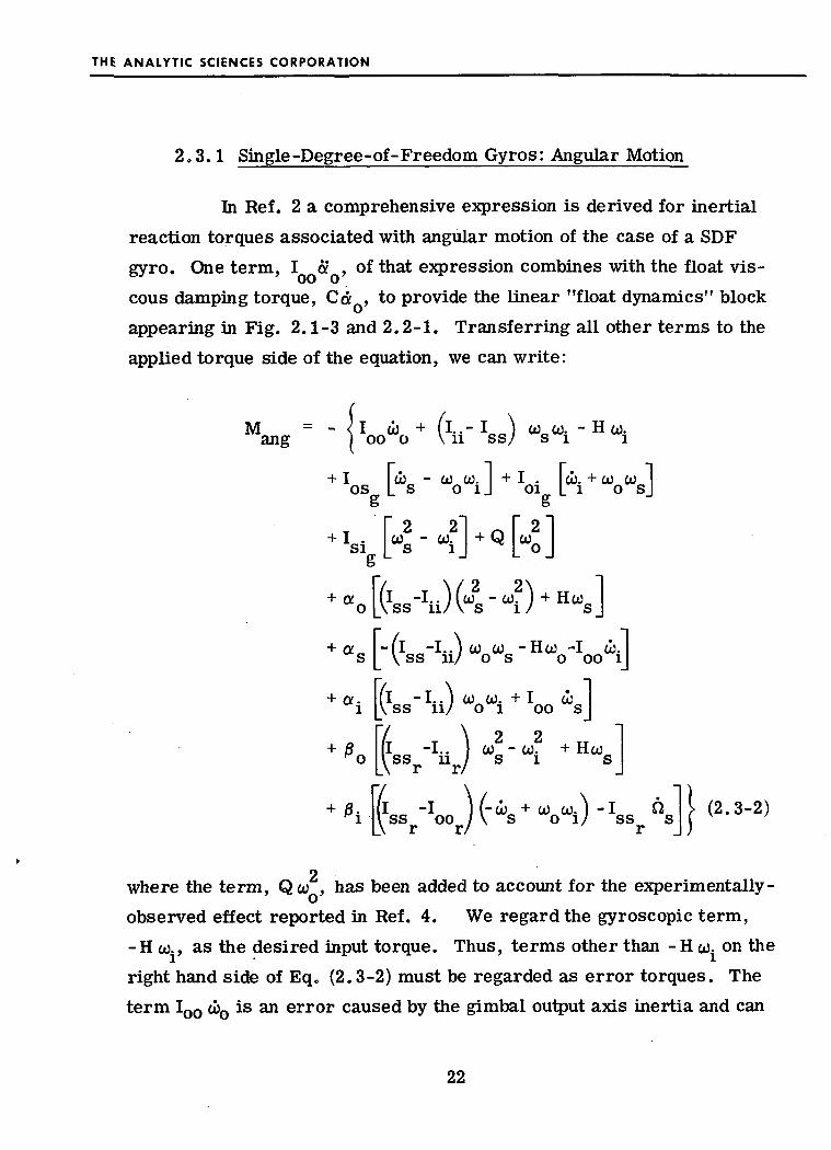
In Ref. 2 a comprehensive expression is derived for inertialreaction torques associated with angular motion of the case of a SDFgyro. One term, I 6? , of that expression combines with the float vis-
7 QQ Q7
cous damping torque, Ca , to provide the linear "float dynamics" blockappearing in Fig. 2.1-3 and 2.2-1. Transferring all other terms to theapplied torque side of the equation, we can write:
Mang
9 2i -i.. w -co +HWss u I s i s
(2.3-2)
where the term, Qco , has been added to account for the experimentally-observed effect reported in Ref. 4. We regard the gyroscopic term,-H to., as the desired input torque. Thus, terms other than - H co. on theright hand side of Eq. (2.3-2) must be regarded as error torques. Theterm Ioo coo is an error caused by the gimbal output axis inertia and can
22

THE ANALYTIC SCIENCES CORPORATION
lead to significant "pseudo-coning" errors in systems applications. The
other term in the first line, (%- Iss) tos wi, is an anisoinertia error tor-que which can lead to large rectification errors during angular vibrations.The product-of-inertia terms in the second and third lines are probablyless important, but can also generate large constant torques. The termsinvolving a are coupling error torques (since a is the float angle whichresults from all applied torques, principally HOJJ) and can also lead to largeerrors. The terms involving Og, c^, BQand /^represent the interaction ofvarious component misalignments with angular motions; the most significantare the -a Hco.. and fi_.Hco_ terms which result when the sensitive axis of the
S O O S
gyro does not lie exactly parallel to the input axis fixed in the case.
2.3.2 Single-Degree-of-Freedom Gyros: Linear Motion
Ref o 2 provides an equation for torques about the output axis ofan SDF gyro generated by linear motion. Based on it we can write:
M.. = - < J m ( 6 f + 6 f. - 6.f + m2
l i n j \ o o s i i s IK f f. + K .f2|_ SO O 1 SI 1
(2.3-3)
Since the only desired torque is the angular motion term, Hco., appearingin Eq. (2.3-2), all of the terms in Eq. (2.3-3) must be considered errortorques. The terms multiplying m have the form of mass unbalancetorques, although the first one, m6 f , is thought to be due to thermalconvection effects. The terms multiplying m^ are linear complianceeffects.
23

THE ANALYTIC SCIENCES CORPORATION
2.3.3 Single-Degree-of-Freedom Accelerometers:Angular Motion
Ref. 3 provides an equation for torques about the output axis
of an SDF accelerometer generated by angular motion. Based on it we
can write:
Mang 'oo^o*11"-
[I -I..o V p p ii
+ 0,
o - to.
(2.3-4)
Since the ideal accelerometer is insensitive to angular
motion, all of the terms in Eq. (2.3-4) must be considered as error tor-ques in the SDF pendulous accelerometer. The error terms can bedivided into several broad categories similar to many exhibited by the
gyro. Sensitivity to angular accelerations is present. The principal con-
tribution, that caused by angular acceleration about the sensor output axis,
is unavoidable because of the nature of the pendulous acceleration sensing
instrument. Several anisoinertia terms and product of inertia terms
also appear.
24

THE ANALYTIC SCIENCES CORPORATION
2.3.4 Single-Degree-of-Freedom Accelerometers: Linear Motion
Ref. 3 provides an equation for torques about the output axis of anSDF accelerometer generated by linear motion. Based on it we can write:
Mlin = *
2 / \ 2lK .f +K f.f + K -K.. f.f -K. f f -K. f > (2.3-5)pi i po i o \ pp ii/ i p 10 o p ip p '' v '
The first term of Eq. (2.3-5), m6 f., measures linearacceleration along the input axis. This is the only output axis torque inthe ideal pendulous accelerometer. The pendulosity m6 is designed intothe instrument with care. All the remaining terms in this equation con-tribute errors to the accelerometer. The term m6 a f is basically ap o pcross-coupling error arising from rotation about the single axis of
freedom and m6 a f results from gimbal-to-case misalignment. Sincep p oaccelerations along the input axis will cause considerable excursions ofthe gimbal angle, a. , from null, sizeable rectification errors can beproduced in this instrument by properly phased linear vibrations withcomponents along the input and pendulum axes. The second term ofEq. (2.3-5) illustrates error torque contributions from unwanted massunbalance and the last line expresses compliance error terms. It can beseen that linear compliance effects can produce constant error torques.The error in indicating linear accelerations along the case fixed inputaxis of an SDF pendulous accelerometer is simply the sum of all errortorques, divided by the pendulosity, m6 .
r
25

THE ANALYTIC SCIENCES CORPORATION
2.4 BASIC PARAMETER GROUPS
In this section the error models given above are specialized andextended slightly. This development is based on approximations which arevalid for the closed-loop sensor configuration with low-frequency testmotion inputs. The motivation for this development is to obtain usefulrelationships in which the disturbance torque is expressed as a functionof motion components and sensor parameters which remain essentiallyconstant over a given period of testing.
The motion-induced error models given above are general inthat they apply to both the open-loop and closed-loop configurations, butthey do not have the desired functional form because of the presence oftime-varying terms a , a , ft and H. The symbol a. represents floato o s oangle which varies in response to all applied torques. The symbol fi
S
represents the rate of change of rotor speed with respect to the gimbalwhich depends on the rate of change of case angular velocity about thespin axis, w , and the rotor speed control loop dynamics.
S
When the gyro is torque rebalanced and can be viewed as aclosed loop system, we can write approximate expressions for a as afunction of certain motion quantities. These can then be substituted intothe above equations to provide the kind of useful functional relationships
mentioned above.
2.4.1 Analog Rebalancing
Consider, first, an analog-rebalanced SDF gyro experiencingangular motion„ For the purpose of computing the float angle, thedominant applied torques can be represented by:
Ma ~= - loo %
26

THE ANALYTIC SCIENCES CORPORATION
The rebalance torque is given by
(2.4-2)
We restrict our attention to low frequency test motions, so that M iskept very small at all times and M, remains an accurate replica ofM „ C on sequently ,a
Therefore,
Mo = Ma - Mtg £ - 'oo^o + HU. + K0o = 0 (2.4-3)
We substitute Eq, (2.4-4)into Eq. (2.3-2)and drop the term 0.1 fi whichis extremely small in practice. The result, after rearranging terms, is:
2M =k < to .+koO! +k0co +k.u).+k.-uj +k_to +k,,u?.ang 1 i <s o 3s 4i 5o 6s 7 i
+k8wo-Vs+k9wiwo+k10wiW8+kllwoWB
3 9 9 9+k19o5. - k19co.co
J.u 1 J. J. i
where k. through k14 are defined in Table 2.4-l(a). We shall call thesecoefficients basic parameter groups. Table 2.4-1 divides them into fourtypes, ji, X , y and p, according to whether they multiply functionsinvolving angular accelerations or functions which are linear, quadraticor cubic in angular rate, respectively. These classifications are usefulin organizing both the analysis and the display of results concerningobservable quantities and testing errors (see Chapter 3).
27

THE ANALYTIC SCIENCES CORPORATION
TABLE 2.4-1
BASIC PARAMETER GROUPS
Angular Motion
a) Gyro
kl = Voo * !oig
k2 = " !oo
V'Voo-'osg
k4 = H
k5= "s"
k6 = - SoH
V V^VO
kg = -Q
Kg = IQS - «i(ISS-I
ii)-Sj(lss -IQO \
^-"/^Oss-'ii)
k!2= («^) Oss - 'ii)
k!3= !ooH/K
k — IT /Vl /¥ T \- . ~ " 11 / I v l l l •" 1. . 1
b) Accelcromctcr
Woo'1,,!
k2 = • ^o
^^-"i^o-'op
k4= V
5 op ) \ pp ii/
6 \ pp ii/
,=-(..-)(,,,„)Linear Motion
c) Gyro
kj = -m6s
k0 = -m6rt£ O
kg = m6.
k4 = -m2Ks.
k6 = -m2Kso
^ = m Kio
d) Accelerometer
k, = -m61 p
k 2=fl pm« p +or im6.
kg = m6j
k4 = -(m2/K)6p6.-m2Kp.
k6=-m2Kpo
2 PP
Type
M
X .
y
P
M
X
y
28

THE ANALYTIC SCIENCES CORPORATION
Except for the fact that H appears in several of them, all ofthe groups defined in Table 2.4-1 are functions of sensor parameterswhich remain essentially constant* over a given period of testing. Wecan write:
where A to represents the deviation of rotor speed with respect to theS
gimbal due to a dynamic lag in the action of the rotor speed control loop.The resulting variations in k,., kg, klfl, k12 and k..,, will cause extremelysmall variations in the corresponding torque components appearing inEq. (2.4-5). These can also be dropped, permitting us to treat most ofthe basic parameter groups as constants. The exception is the gyroscopicterm, Hw,, which becomes:
Hco. = H w.+1 AO w. (2.4-7)i nom i ss si v 'r
We have assumed here that float axis misalignments (ai, as and ap)and rotor axis misalignments (0j and 0O) are constant. If future resultsindicate that these quantities significantly vary due to case motions, theonly changes in this development which are likely to be significantinvolve the kg and kg terms in Eq. (2.4-5) and the k£ term in Eq. (2.4-15).The affects on kj, k3, k?, kg and k^ in Table 2.4-l(a) and on kj_, k3, kgand k7 in Table 2.4-l(b) will be very small if the misalignments are of theorder of arc seconds.
29

THE ANALYTIC SCIENCES CORPORATION
The second term in Eq, (2.4-7) is zero except when the applied test
motion involves both w. and a rapidly varying co . Therefore, most of1 S
the time the parameter groups defined in Table 2.4-l(a) can be con-
sidered constants with H = H . For example, with a vibratory angularn o m ' j omotion about the spin axes, if the frequency of vibration is low compared
to the wheel hunt frequency (typically a few cycles per second), Afi = 0S
and Hco, = H o>.. If, on the other hand, the frequency of oscillation is
considerably above the wheel hunt frequency, the rotor speed variation
will become:
A Q0 = - co0 (2.4-8)b S
That is, to is varying so rapidly that the speed control loop cannot followS
it at all (see the more extensive discussion in Ref. 2). Consequently,
= Hnom<"i -
and the "extra" term can be added to the k lnw. w term in Eq. (2.4-5).JLU 1 S
In summary, all of the parameter groups defined in Table 2.4-l(a) can
be considered independent of test motion frequency except k.., which
varies from:
30

THE ANALYTIC SCIENCES CORPORATION
for angular oscillations about the spin axis which are well below thewheel hunt frequency, to:
k = \-~Z] + I -I -I.. (2.4-11)1Q 1 If i \ oe» do it / x /
for oscillations well above the wheel hunt frequency.
The expression of the applied torque in the form of Eq. (2.4-5)leads to a testing concept in which the data processing portion of the testprocedure is divided into two parts. In the first part the gyro output datafrom a sequence of tests is processed so as to determine values of thebasic parameter groups. The second part is a purely algebraic problemin which the basic parameter groups are provided and the individualparameters appearing in the expressions in Table 2.4-1 are to be extracted.
The first phase is crucial because it bears on the choice of testmotions and determines test accuracy and useful test duration. Note,for example, that some basic parameter groups appearing in Eq. (2.4-5)cannot possibly be found by applying a constant rotation rate since theymultiply angular acceleration terms (d^, wo, u>s). This indicates that ifall parameter groups are to be determined, the testing program mustinclude some motions more complex than constant rates.
In the second phase some of the parameters can be foundalgebraically and some cannot, but there is no way in which unusual testmotions can be used to separate the effects of individual parameters which
31

THE ANALYTIC SCIENCES CORPORATION
appear in a given group. For example, consider the single term from
Eq. (2.4-5) involving the product, to to .o s
lss
No matter what time history of u and co_ is applied to the gyro case, theO ID
term involving IOj and the term involving a will both remain proportional
to the product, to to , and their separate effects cannot be distinguished.o sHowever, if values for both kj and k^1 (see Table 2.4-l(a)) have been
determined, and if I and (IQC - L<) are considered known, then valuesoo °° Li
for IOi and a can be determined algebraically.5
It should be noted that we could have started with an expression
like that of Eq. (2.4-5), without assuming any knowledge of the physical
causes of error torques, and simply set out to design a testing procedure
which would determine values of the coefficients of the various motion
functions. This corresponds to the first approach mentioned in
Section 2.2.
For an SDF accelerometer basic parameter groups defined in
Table 2.4-l(b) correspond to the following expression for torque due to
an angular motion:
2 2M = k. co. +kqco +k_w +k.co. -k.toa n g 1 i T J o 3 p 4 i 4 p
+ kcco.co +kcco-oo +k_u3 oo +k0ci5 co -k0co o>5 i o 6 i p 7 o p 8 0 1 S o p
(2.4-13)
32
THE ANALYTIC SCIENCES CORPORATION
where we have made use of the approximation:
I
«0 =" - -r. *„ (2-4-14>
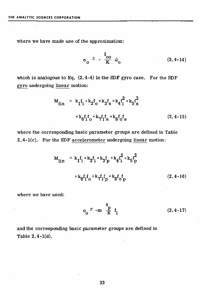
which is analogous to Eq. (2.4-4) in the SDF gyro case. For the SDF
gyro undergoing linear motion:
Mlln
+ ViVk7fi£s+WS <2'4-
where the corresponding basic parameter groups are defined in Table
2.4-l(c). For the SDF accelerometer undergoing linear motion:
Mlln
+ Vifo+k7£iWof
where we have used:
= -m - f. (2.4-17)
and the corresponding basic parameter groups are defined in
Table2.4-l(d).
33

THE ANALYTIC SCIENCES CORPORATION
2.4.2 Pulse-Rebalancing
The basic parameter groups defined in Table 2.4-1 may be
valid for some pulse-rebalanced sensors as well, even though Eq. (2.4-2)
is no longer true. In some cases the float angle, a , experiences a high-
frequency limit cycle* superimposed on a slowly changing "signal" value
which follows quite closely the applied test motion. According to dual-
input, describing-function theory (Ref. 5) the nonlinear torquing logic
operates on these low frequency signals, which occur in the presence of
the limit cycle, almost as though it were a linear gain. Therefore, we
can write:
M = - M, = -K N_ K. a (2.4-18)a tg sg B tg o v '
where:
K = the signal generator gain
K, = the torque generator gain
NR = the effective gain of the nonlinearityas seen by the "signal".
and the overbars indicate time-averages taken over intervals which
are long compared to the limit cycle period but short compared to
*This is usually true in the binary-torquing case and for gyros with
time-modulated torquing; it is usually not true in the ternary-torquingcase. See Ref. 2.
34
THE ANALYTIC SCIENCES CORPORATION
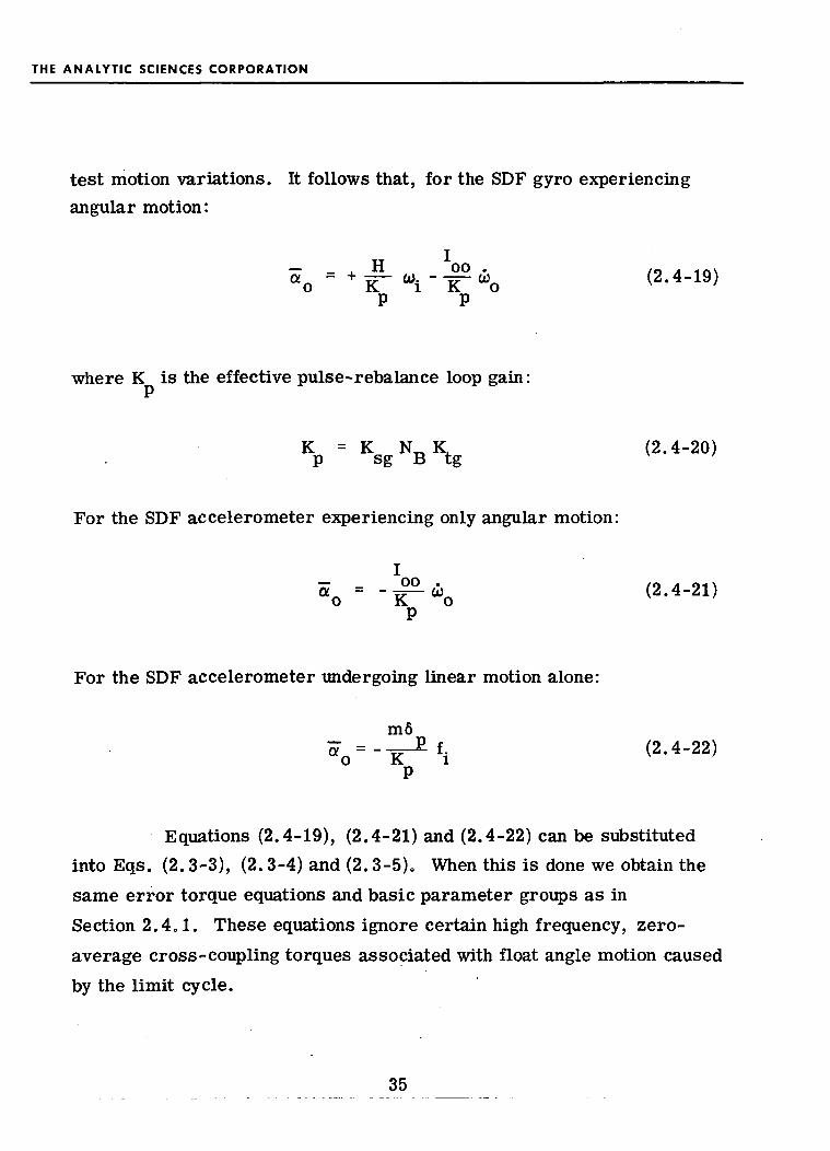
test motion variations. It follows that, for the SDF gyro experiencingangular motion:
OO . fn A -tr\\w (2-4-l9)p
where K is the effective pulse-rebalance loop gain:
K = K ND K. (2.4-20)P sg B tg '
For the SDF accelerometer experiencing only angular motion:
<2-4-21'
For the SDF accelerometer undergoing linear motion alone:
m6
V-K^ f iP
Equations (2.4-19), (2.4-21) and (2.4-22) can be substitutedinto Eqs. (2. 3-3), (2. 3-4) and (2. 3-5)= When this is done we obtain thesame error torque equations and basic parameter groups as inSection 2.4, 1. These equations ignore certain high frequency, zero-average cross -coup ling torques associated with float angle motion causedby the limit cycle.
35

THE ANALYTIC SCIENCES CORPORATION
2. 5 TEST MOTION POSSIBILITIES
In order to determine values for all basic parameter groups
appearing in Eqs. (2.4-5), (2.4-13), (2.4-15) and (2.4-16) it is necessary
to choose a sequence of test motions which excite the various terms in
these equations in such a way that their individual effects can be separated
and measured. An important consideration in this choice is the desirability
of keeping the test motion equipment as simple and accurately controllable
as possible. For the angular motion-induced terms of Eqs. (2.4-5) and
(2.4-13) it is necessary to specify a set of time histories of angular
velocity components (u>j, coo, U3S). These cannot be confined to constant-rate tests alone since there are a number of terms involving angular
accelerations (cbj, coo> tos ) which must be excited. For the linear motion-
induced torques of Eqs. (2.3-15) and (2. 3-16) it is necessary to specify a
sequence of specific force (fi? fo, fs) time histories.
Consider the following list of possible motion functions which
are discussed, in turn, below:
• Step functions (constant angular rates and constantspecific force components)
• Ramp functions (constant angular accelerations)
• Sinusoidal oscillations (angular and linear vibrations)
(a) motion about or along a single case-fixed axis
(b) oscillations about two axes with arbitrary phase
(c) oscillations about three axes with arbitrary phases
• Combinations and special functions
Note that two- and three-axis in-phase oscillations are actually single-
axis oscillations where the axis is chosen to produce a specified ratio
between principal axis components. (For example, angular oscillation
36

THE ANALYTIC SCIENCES CORPORATION
about a line midway between the input and spin axes of a gyro with rateW sin cot, produces the principal axis in-phase oscillations,co. = co_ = (W/,/2~) sin cot.i s
Constant angular rates may be applied to inertial sensors byconventional laboratory test tables. Special mounting fixtures arerequired for various "combined-rate" tests. For example, if equal input-axis and spin-axis rates (coj and cog) are desired simultaneously, thegyro must be mounted with the line midway between these two axes coincidentwith the test table axis. Constant specific force components may be obtainedsimply by placing the sensor in a given orientation in the earth's gravi-tational field. Alternatively, it may be centrifuge tested at a higher g-level. (This produces a combination of constant angular rate about thecentrifuge axis and a constant specific force, somewhat complicatingmatters.) These tests are all useful and are commonly performed intesting inertial sensors. Their major limitation is that, in testing forangular-motion-induced errors, they cannot excite all of the terms appearingin the error model equations. It is clear, therefore, that some test motionsfrom the last three items in the above list should be included in a completetesting program.
Angular-rate ramp functions, involving constant angularaccelerations, could be used to excite the terms which are not excited inconstant rate testing. Supplying such motions would require the operationof standard test tables in an unconventional way, and it would be difficultto maintain a significant acceleration level for a long period of timebecause of the high rates which would be reached. There would also beserious data processing problems because of the continuously increasingtorque levels associated with various parameter groups. For example, aconstant angular acceleration about a gyro output axis would cause a
37

THE ANALYTIC SCIENCES CORPORATION
constant torque, luco- [See Eq. (204-5).], and a linearly increasingtorque, kgujQ, and a parabolically increasing torque,
Angular and linear single-axis sinusoidal oscillations are
standard test motions which may be obtained using conventional techniques.Since first and higher derivatives automatically occur as sinusoids, allterms in the error models can be excited by a sequence of sinusoidaloscillations about various axes. As with ramp functions the torque levelsduring sinusoidal motion are continuously changing. However, they arecyclically repeating, affording the opportunity to average data over manycycles. The data processing procedures required to separate and measurethe effects of various parameter groups during such testing are developedin some detail in Chapter 3. (They represent a considerable increase overthose usually employed in test procedures which seek only to measureaverage effects. ) It is demonstrated that a particular sequence of sixsingle-axis vibration tests, each using a different test motion axis fixedin case coordinates can theoretically be used to isolate and measure allterms which appear in the error models we have adopted. (Some effects,such as torques associated with k12 and k..., are extremely small andprobably cannot be measured in practice in low frequency testing. But ifthey are too small to be measured, they are also likely to produce insig-nificant errors in operational systems. On the other hand these effectsshould be reviewed in later considerations of high frequency testing. )
Because a program of single-axis testing which includes constantangular rates and oscillatory motion has the capability mentioned above,multi-axis out-of -phase testing and angular rate histories which arecombinations and special functions of time have not been studied in detail.Multi-axis test tables capable of supplying out-of-phase angular motions
38

THE ANALYTIC SCIENCES CORPORATION
are available and these should, of course, be used to check againstpredictions based on single-axis testing. However, a major conclusionof this study is that for strapdown inertial sensors considerable emphasis
should be given to single-axis low-frequency testing.
The ultimate simplicity and usefulness of single-axis low-
frequency testing will depend on the extent to which:
• all motion-affected error torques, including thosenot covered in the error models presented here,are frequency independent.
• It is valid to treat pulse rebalancing electronics aslinear components in the fashion outlined inSection 204.2.
• it is possible to predict the significant system errorsfrom the results of single-axis low-frequency tests.
A combination of experimental evidence and further analysis is needed
in order to properly guage these matters.
Chapter Summary — Error equations for single-degree-of-freedom (SDF) gyros and accelerometers are developed for the specialcase of closed-loop low-frequency testing. The resulting expressions fortorques applied to the instrument output axes are linear in a set of "basicparameter groups" defined herein. The expressions for angular-motion-induced error torques include fourteen such parameter groups for SDFgyros and eight groups for SDF accelerometers. The expressions forlinear-motion-induced error torques include eight groups for both SDFgyros and accelerometers. The parameter groups are further dividedinto four categories, according to whether they generate error torquesproportional to angular acceleration or linear, quadratic or cubic,
39

THE ANALYTIC SCIENCES CORPORATION
respectively, in angular rate or specific force. These classificationsare useful in organizing both the analysis and the display of results
developed in the following chapter.
Potential test motions are reviewed and qualitatively comparedin light of the applied torque expressions mentioned above. A major con-clusion is that theoretically the effects of all parameter groups can beobserved separately using test motions which involve angular accelerations;it is not necessary to resort to multi-axis, out-of-phase test motions.
40

THE ANALYTIC SCIENCES CORPORATION
3. SINGLE-AXIS, LOW-FREQUENCY TESTING
This chapter presents a detailed study of single-axis, low-frequency testing, including sinusoidal vibration testing and constantangular rate testing. A particular set of sensor orientations with respectto the motion axis are recommended and the information which may beextracted from each test is outlined for angular and linear vibration testsas well as constant rate tests. Test accuracy, useful test duration andtest data processing are investigated, with emphasis on the angular motioncase. Example calculations are given at the end of the chapter.
3.1 OBSERVABLE QUANTITIES
This section identifies the quantities which may be observed asa result of single axis tests and the basic parameter groups which may bedetermined from the quantities observed during particular types of testsequences and combinations thereof„ The following types of tests are
considered:
• Constant Rate Testing
• Sinusoidal Testing, Averaging
• Sinusoidal Testing, Harmonic Extraction
The last two involve the same test motions, but are distinguished by the dataprocessing performed. In sinusoidal averaging the only measurement is ofthe average torque over many cycles, yielding information about constant
41

THE ANALYTIC SCIENCES CORPORATION
torque only, part of which is due to rectification of dynamic effects. In
sinusoidal harmonic testing the time-varying output signal is processed
to yield additional information. Results are summarized in
Section 3.1.3.
3.1.1 Vibration Testing
A general single-axis angular vibration of amplitude W and
frequency co can be represented by the following three equations:
co. = c. Wsin cot (3.1-1)
03 = c Wsin cot (3.1-2)o o
03 = c Wsin tot (3.1-3)s s
where c., c and c are the direction cosines relating the vibration axisr o sto the input, output and spin axes of the gyro being tested. It is shown in
Appendix A that when Eqs. (3.1-1), (3.1-2) and (3.1-3) are substituted
into Eq. (2.3-5), the resulting expression for applied torque is a periodic
function represented by a 7-term trigonometric series of the form:
M = B + S. sin o)t + C, cos o>tang 1 1
+ S- sin 2o>t + C2 cos 2ojt
sin 3o)t + C cos 3o)t (3.1-4)
42

THE ANALYTIC SCIENCES CORPORATION
When three similar equations representing accelerometer case motion(involving u> and c rather than co and c ) are substituted into Eq. (2.3-5),P p s sa similar periodic function of the form of Eq. (3.1-4) is found. Thisresult is also developed in Appendix A. In both cases, expressions forthe coefficients, B, S., CL, etc., in terms of the basic parameter groupsand the quantities defining the test motion have been derived.
Figure 3.1-1 illustrates the general situation for a single-axisangular vibration test. The first block represents the motion-inducedtorque model developed in Section 2.4; its output, M , can be viewedas a 7-term periodic function of the form of Eq. (3.1-4). Added to this isa constant torque, M , which exists in the absence of the applied angularvibration. It consists of the terms, M,. and M,. , defined in Eq. (2.3-1)bias 1m ^and a small additional torque due to the angular rotation rate of the earth.Since the only applied test motion is an angular oscillation, the linear-motion-induced torque is determined by the sensor's orientation in theearth's gravitational field., This torque can be held constant by orientingthe vibration axis or "test axis" in the vertical direction. The completeapplied torque, M , is, therefore, also represented by a 7-term function
3.
of the form of Eq. (3.1-4) in which the bias coefficient, B, includes theconstant, Mc, as well as the average (rectification) torque resulting fromthe applied sinusoidal angular motion. Since the test motion frequency hasbeen assumed to be low compared to gyro loop dynamics, the torquegenerator output is represented by the same 7-term function. The gyrooutput e is a scalar function which is proportional (ideally) to the torqueM, . Therefore, a harmonic analysis of the output data should produce theseven Fourier coefficients which define the input periodic function M (t),
3-
For any given choice of sensor orientation with respect to the test axisthere is a set of seven such coefficients which are the observable quantities
43

THE ANALYTIC SCIENCES CORPORATION
e-258
a)0=c0Wsinajt.
ait
Mc
Functionwhich is
nonlinear in
but linearin basicparameter
groups
+>+ X1
->K.'M0
\l/~./ *"+ V.
"j
M,g
>k ^_
J >•
k
FloatDynamics
TorqueGenerator
*"
1,'Sigr
Gentlal>rator
e,Data
Processing
B
Ic,
c'2S3
_ 3.
Figure 3.1-1
M,g= M0-B + S,sin wt + C, cos ait
+ S2sin2a>t+C2cos2<u
+ S3 sin3a)t +C3cos 3w
General Single-Axis Angular Vibration Test
for that particular test. Estimation of these seven quantities requires amore sophisticated data processing procedure than the conventional one ofmeasuring average drift rate over a long period of time (which is simplythe measurement of B, the first of the seven coefficients).
Consider now the six test orientations pictured in Fig. 3.1-2.In three cases the sensor is mounted with one of its principal axes coinci-dent with the test motion axis. In the other three cases the sensor ismounted with a line midway between two of its principal axes coincidentwith the test axis. These pictures apply to a SDF gyro or SDF accelerom-eter, depending on whether the third principal axis is labeled s or p.Tables 3.1-1 and 3.1-2 present expressions for the seven trigonometriccoefficients which correspond to each of these six test axis choices for bothinstruments. Each Fourier bias coefficient, B, includes a constant torqueterm, M , which represents the disturbance torque which exists in the
\^
absence of the test motion. It is a function of orientation, temperature, etc.
44

THE ANALYTIC SCIENCES CORPORATION
R-805
TEST MOTION AXIS
( tma) tma tma
s,P
f ma tma tma
s,P
s,P
s,P
Figure 3.1-2 Six Candidate Test Orientations
45
THE ANALYTIC SCIENCES CORPORATION
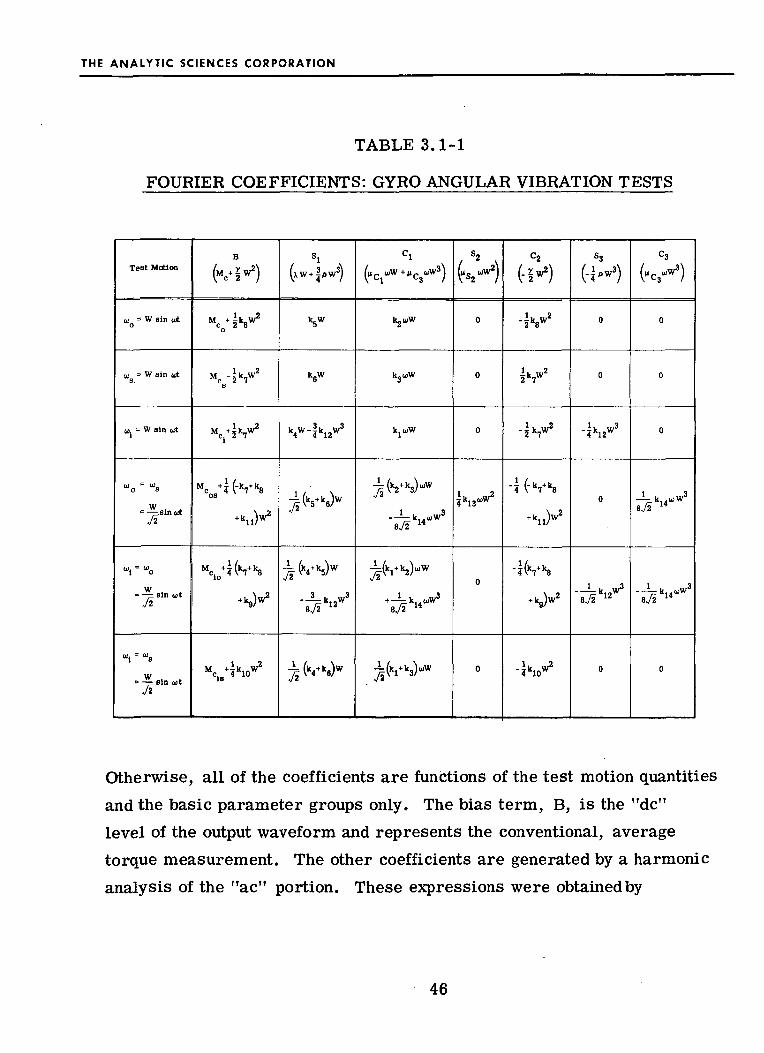
TABLE 3.1-1
FOURIER COEFFICIENTS: GYRO ANGULAR VIBRATION TESTS
Test Motionl
(xw+|pw3)
S2
a " W sin u* - k W2K8W
u = W sin wt
W sin wt
k w
-4 12
W= -^sin ut
72
"I (-Vk8
872 14o)W
W— sin wt72
W3
W— sin at72
- 2-
Otherwise, all of the coefficients are functions of the test motion quantities
and the basic parameter groups only. The bias term, B, is the "dc"level of the output waveform and represents the conventional, averagetorque measurement. The other coefficients are generated by a harmonicanalysis of the "ac" portion. These expressions were obtained by
46

THE ANALYTIC SCIENCES CORPORATION
TABLE 3,1-2
FOURIER COEFFICIENTS: ACCELEROMETER
Test Motion
u> = Wsinuto
a) = WsinwtP
cu. = Wsinojt
w= -5- sinwt
0). = U>Q
w= — sin uit
0). = W1 P
= — sin cut
ANGULAR VIBRATION TESTS
B
\
MCp-ik4W2
M^^W2
cop 4 7
%-.v^
•S, -1
fe,.w?U.-)
Vw
"s-k,.w
.~_ /'lr l lr ^ / 1^X7^ lr * tW
/~K" \ A O/ o /~n~ "
1 1 3
^ k l + k 2 W W + «^VW
^(kl+k3)«*W
C2
0
K*2
4^
te-^
i(k. -Ow24V 4 5/
-h^
C3
0
0
0
1 1
8/T 8
. . _.,. .., lr , A\?
8/T ^
0
specializing the general expressions derived in Appendix A. For example,
for a test motion axis midway between the input and output axes we have:
c4 = 1A/2
CQ = 1/72
Cg = 0 (3.1-5)
47

THE ANALYTIC SCIENCES CORPORATION
Therefore, in the case of the gyro, the expression for the coefficient ofthe sin 3 cct term [Eq. (A-5(f)] becomes
I k r - c4 *12 W \Ci Cis
(3-1-6)
The output data from a sequence of six tests on a given instru-ment can be processed to yield an array of 42 observable quantities. Ifthe six test axes are those pictured in Fig. 3.1-2, the 42 quantities cor-respond to the expressions given in Table 3.1-1. Examination of thisarray of expressions shows that, for a given test amplitude and frequency,knowledge of these 42 quantities is more than enough to determine all ofthe basic parameter groups, kj through k... All six tests are required,but the complete set of 42 observables provides a considerable amount ofredundant information. The testing concept outlined in Section 2.4 can nowbe made more definite as shown in Fig. 301-3. The gyro data may beprocessed (stage la) on-line to produce the seven observable quantities(Fourier coefficients) during each test or it may be recorded for sub-sequent off-line processing. In either case, the next data processingstage, Ib, is an off-line stage in which 42 linear algebraic equations are tobe solved for 20 unknowns; 14 basic parameter groups and 6 constant tor-ques, M . Approaches to the solution of this over-specified problem are
\*>
discussed briefly in Section 3.4. The final data processing stage, II, isthe purely algebraic problem of solving for individual parameters, givenvalues for the basic parameter groups.
48
THE ANALYTIC SCIENCES CORPORATION
Sequenceof Six
VibrationTests
SensorOutput
>•
Data Processing
Phase la/ on-line \[ o r IVoff -line/
Array of 42Coeff icients
Data Processing
Phase Ib
(o f f - l i ne )
basicParameter
Groups^
Data Processing
Phase H
(o f f - l i ne )
Indivi dual
Parameters
Figure 3.1-3 Data Processing Phases: Single-Axis Vibration Testing
Table 3.1-3 presents expressions for the observable quantities(Fourier coefficients) which correspond to linear vibration tests in whichthe vibration axis has the same relationship to the sensor axes as in thesix angular vibration tests described above.* For these linear vibrationtests the test axis is chosen to be horizontal so that the specific force alongthe test axis has a sinusoidal form with zero average. The constant tor-que, M,., includes the usual bias term, M, . , a small term, M ,^ ' c' ' oias' ang'associated with the constant earth rate and a term associated with theconstant gravitational field. The number of observable quantities for eachtest is three, corresponding to three-term trigonometric functions whichare derived in Appendix A for single-axis linear vibration tests. In bothcases (gyro and accelerometer) the set of 18 observable quantities is morethan enough to determine all basic parameter groups.
Inspection of the expressions tabulated in Tables 3.1-1 through3.1-3 reveals that, for both SDF gyros and SDF accelerometers, completesets of basic parameter groups may theoretically be extracted from asequence of six angular and six linear vibration tests. The angular
In the case of the gyro it will be extremely difficult in practice tomeasure the mass unbalance terms (kj, k2, kg) because of the smallangular motions which must inevitably be present. Extraction of thesecoefficients is performed quite satisfactorily during simple tumble tests.
49

THE ANALYTIC SCIENCES CORPORATION
TABLE 3.1-3
FOURIER COEFFICIENTS: GYRO AND ACCELEROMETER
Test Motion
a = Asinwt
a = Asinwt
a. = A sin u't
= — sin tot
ai =ao
= sin (1.1 1
ai =as
= sin u»t
LINEAR VIBRATION TESTS
B
\
-..*»*•*'
V*"**"
cos
M _L _ _ f Ir -)- lr i AA \ A ^ I **c . s 4^4 e;
%+Jh^^)A'
Sl
(XA)
V
v
k,A
-(v,)A
^^^*$w
I c^2}0
1, .2'2k5A
1 2
-Jh^A"
-fr,",)*1
-Kvv^
vibration tests should be conducted with the vibration axis (about which the
sensor is rotated) in the vertical direction. The linear vibration testsshould be conducted with the vibration axis (along which the sensor is
accelerated) in the horizontal plane.
50

THE ANALYTIC SCIENCES CORPORATION
3.1.2 Constant Angular Rate Testing
When a constant angular rate is applied about any axis fixed inthe sensor, the resulting applied torque is a constant. A general constantrate of amplitude W can be represented by the equations:
ooj = ctW (3.1-7)
WQ = CQW (3.1-8)
WSD = c s i> W (3>1-9)&,p s,p
For any values of the direction cosines the resulting expression for the
applied torque (see Eqs. (2.4-5), (2.4-13) and (2.3-1)) takes the generalform:
M = M + XW + yW2 + pW3 (3.1-10)a c
Table 3.1-4 expresses the coefficients, X, y, and p, in terms of basicparameter groups for the six test motion axes shown in Fig. 3.1-2. Ineach case the M term represents the constant torque which exists in theabsence of an applied angular rate (i.e., when W = 0). For each test axisit is necessary to measure torque for three non-zero values of W in orderto separate X, y and p terms.
Inspection of the left hand (gyro) side of Table 3.1-4 shows thatestimates of the X terms lead directly to estimates of the parameter groups,k,, kg and kg, and estimates of the y terms lead to the groups, k^k^kg,^,,
and kt . For accelerometers the X terms do not appear while the y terms lead
to estimates of the groups, k4,k5,kg and k7. (These groups are defined in
Table 2.4-1.)
51

THE ANALYTIC SCIENCES CORPORATION
TABLE 3.1-4
APPLIED TORQUE EXPRESSIONS: CONSTANT RATE TESTING
TestMotion
»o = w
"s,P = W
w. = W
/ . - , i - w / /~5~o s, p
r 1 — / * — W/ / 9
i o
_ _ w / ro~1 Sj p
M
M +MOS
Tk +k4M , ^
cio L/2-
ci
M = M + XW + y W + pWa c
Gyro
o
s
, + k4w + k?w2 + k12w
3
\v + ^ ^ ^ w2
L VT J ' L 2 J "
1 ' k + U + k l f i r 17 fl Q 9 19 T
W I \V I W
i k4+kel\v i fkl°l\v2
s /T 2
Accelerometer
Mco
cpM + k . W 2
c. 4
M I t ,,,&Mc oop L ^
C. 01O "
kfi 9M + b W*2
Cip 2
3.1.3 Summary: Angular Motion Test Observables
Table 3.1-5 identifies the gyro parameter groups which may bedetermined as a result of each type of testing considered. A sequence ofconstant rate tests is capable of determining all groups except the so-called"/n terms" (k. jk^k^k..,, and k14), which are associated with angularacceleration. A sequence of sinusoidal averaging tests is useful only indetermining the "y terms" (k7,kg,kg,k10 and k^). A sequence of sinus-oidal harmonic tests is capable of determining the full set of parametergroups, as previously discussed. Thus, a combination of constant rate
52

THE ANALYTIC SCIENCES CORPORATION
TABLE 3.1-5
DETERMINABLE GYRO PARAMETER GROUPS:ANGULAR MOTION TESTING
u terms
kl' k2' k3' k!3' k!4
X terms
k4' k5' k6
y terms
k7' k8' V k!0' kll
0 terms
k!2*
Number of runs required
Constant RateTesting
M -M = XW+yW2+pW3
a c
No
Yes
Yes
Yes
12, (15)
SinusoidalTesting,
AveragingB = Mc+iyw2
No
No
Yes
No
6
Sinusoidal Testing,Harmonic Extraction
S j = X W C 1 = ( *uW
S^j^W2 C^-JyW3
S^JpW3 C'^wW3
Yes
Yes
Yes
Yes
6
"Very small: probably unobservable In practice.
tests and sinusoidal averaging tests yields no more groups than those foundin constant rate tests alone, but does provide independent measures of they, or rectification, terms. Similarly, a combination of sinusoidal harmonictesting with the other types yields no more groups than those found inharmonic testing alone, but does offer the advantage of independent measure-ments of X, y and p terms and, therefore, additional cross-checkingopportunities. The relative accuracies of the different testing methods arecompared in Section 3.2.1.
53

THE ANALYTIC SCIENCES CORPORATION
As illustrated in the numerical examples of Section 3. 5, theparameter groups k12 and k.. . are expected to be extremely small. It is,therefore, likely that the cubic terms (pterms) in constant rate testingand the third harmonic (83 and €3) in sinusoidal testing can be ignored inpractice. It is also worth noting that both k. and k^ are approximatelyequal to IO4 and that both k_ and kQ are approximately equal to Ios .S «J y gConsequently, there may be fewer significant quantities that cannot bemeasured during constant rate testing than is suggested by Table 3.1-5.
Table 3.1-5 also shows the number of test runs required in eachsequence. The constant rate tests will probably require two non-zero ratesfor each of the six test axes shown in Table 3,, 1-2 in order to separate theX and y terms, making a total of 12 runs. Theoretically, a third rate isrequired for the three test axes where a cubic (p) term appears, making atotal of 15 required runs. In practice the cubic terms will probably beignored. The number of runs listed in Table 3.1-5 under constant ratetesting is 24, rather than 12, because each set may be repeated with thesensor re-mounted after a rotation of 180 degrees about the test axis. Thiswould be done in order to correct for a misalignment of the table axis.
Sinusoidal testing entails only one run for each of the six testaxes, making a total of six required runs. In practice, for sinusoidalharmonic testing each test will probably be repeated with the sensor re-mounted, as described above. Therefore, the number of required runs isstated as 12. The number 6 is maintained for sinusoidal averaging sincetable axis misalignment does not cause a constant error torque.
Under the assumptions of our error models (all parameter
groups independent of test motion, etc.) no new information is gained byrunning a sinusoidal test at varying frequencies or amplitudes. In
54

THE ANALYTIC SCIENCES CORPORATION
practice, of course, it would be desirable to vary these test motionquantities in order to check the consistency of the results and to see ifand where the error model breaks down.
3.2 SINGLE-AXIS TEST ACCURACY
Procedures which involve sequences of single-axis tests wereoutlined in the previous section. The objective of these test sequences isto obtain measurements of a set of basic parameter groups which causemotion-induced error torques. The measurements cannot be perfect for anumber of reasons. The sources of test errors are analyzed in this sec-tion and relationships between error sources and test accuracy are
developed.
3.2.1 Overview and Comparison
Test error categories are listed in Table 3.2-1 and discussedbriefly below. More detailed discussions are given in following sections.It should be noted that "measurement errors" are associated with the tor-que rebalance path of the gyro itself, which is used to determine the natureof the applied torque time history. "Motion errors" are associated withimperfections in the motion supplying devices.
Table 3.2-1 indicates which tests are significantly affected byvarious types of test error. A zero entry in the table implies that thesource in question is expected to contribute negligibly small errors to
55

THE ANALYTIC SCIENCES CORPORATION
TABLE 3.2-1
TEST ERROR INFLUENCES
Test Error Categories
Test Motion Errors
Magnitude
1. Bias
2. Waveform Distortion
3. High -Frequency Noise
Misalignment
4. Bias -Fixed
5. Run-to -Run Shift
6. Table Wobble
Measurement Errors
7. Quantization
8. Torquer Scale Factor Error
9. Torquer Nonlinearity
10. High- Frequency Noise
Parameter Changes
11. Run-to-Run Shifts
ConstantRate
Testing
0
NA*
0
X
x,yx,y
x,yx,yx,yx,y
x,y
SinusoidalAveraging
y0
y
0
NA
0
yyyy
NA
SinusoidalHarmonicTesting
M,y11 *V
f 1 3k *V
X
NA
M
If *i *V^ J J '
II \ *V
If 1 *Vr"> ? '
• i Jk <y
NA
NA = Not Applicable.
56

THE ANALYTIC SCIENCES CORPORATION
estimates of the parameters in question. An "NA" entry stands for "notapplicable." For example, distortion of the applied test motion waveformis not a problem for constant rate tests. A Greek letter or lettersappearing at a particular location in the table indicates which types ofcoefficients will suffer significant estimation errors due to the errorsource in question. The following paragraphs provide brief discussions ofvarious test error source categories and references to detailed treat-ments in succeeding sections.
Test motion bias errors are constant errors in the knowledge ofthe applied test motion amplitude or of the orientation of the test axis.Test motion bias errors change the values of the observable quantitiesbeing measured. Since calculation of sensor parameters is based onassumed test motions which are different, they are in some error. Theseeffects are discussed in detail in Section 3.2.2 and Appendix B. Theerror in the knowledge of test motion amplitude, in constant rate testing,is expected to be negligibly small because table rate is determined from ameasurement of the total time required for an integral number of testtable revolutions; this can be done very accurately. The effect of a fixedtest axis misalignment error on the JLI and y terms during sinusoidaltesting is negligible, as shown in Section 3.2.2. A shift in the misalign-ment error between two constant rate tests, for a given test axis orientation,affects both the A and y estimates, as shown in Section 3.2.2.
Cyclically repeating test motion errors, such as table wobble ordistortion of the applied sinusoidal motion, give rise to harmonics in theapplied torque time history. In constant rate testing the table-wobbleeffects may rectify and change the average torque measurement. Theseerrors are discussed in Section 3.2.3. Other examples of cyclic testmotion errors are linear vibrations occurring during angular vibration
57

THE ANALYTIC SCIENCES CORPORATION
tests (due to an off-center test axis) and angular vibrations occurringduring linear vibration tests (due to unwanted "rocking" motion). Theformer might be significant when subjecting an accelerometer to angularvibration testing; the latter will be very significant when subjecting a gyro
to linear vibration testing.
Errors due to quantization can arise in testing analog-rebalancedsensors as well as pulse-rebalanced sensors. In the first case this willhappen whenever the continuously varying torquer input signal is converted
into digital form for data processing. As with a pulse-rebalanced sensor,the test data becomes a sequence of integers (pulse counts) which representthe integral of torque over particular time intervals. One count representsthe basic quantization interval or data resolution level in units of torque-times-time (e.g. dyne cm sec). All parameter estimates are affected by thisquantization. This problem is discussedin detail in Sections 3.2.4 and 3. 2.5.
Random high-frequency fluctuations in the applied test motion canbe viewed as "process noise" affecting the entire test procedure. Thistogether with similar fluctuations in measurement errors or "measurementnoise" places a limit on the achievable parameter estimation accuracies.In some cases the quantization process is effectively a contributor to mea-surement noise. Besides that contribution there is the difference betweenthe actual physical torque generated (or its integral over an interval) andits indicated value. All Fourier coefficient estimates are affected by theseerrors. They are discussed in Section 3.2.6 and Appendix C. In the caseof constant rate testing, while the applied rate may fluctuate about itsaverage value, the average will be known with negligible error, as dis-cussed above., The first order effect on the estimated parameters willalso be negligible since the integrated effect of positive deviations willexactly counteract the integrated effect of negative deviations.
58
THE ANALYTIC SCIENCES CORPORATION
Cyclically repeating measurement errors are the result of fixedrebalance loop errors such as torquer nonlinearity or torquer scale-factorerror. The "odd-nonlinearities" affect constant rate testing and themeasurement of the \i terms in sinusoidal harmonic testing. The "evennonlinearities" affect sinusoidal averaging and the measurement of the Xand y terms in sinusoidal harmonic testing. These effects are discussedin Section 3.2.7.
The shift in sensor parameter values between two constant ratetests with a given test axis orientation affects both the X and y estimates,in much the same way as a shifted misalignment error affects them. Theseeffects are discussed in Section 3.2.8.
Table 3.2-2 repeats the format of Table 3.2-1, but suppliesmore detail in the form of error formulas. These formulas express theerrors in estimating the /j, X and y terms as functions of the error sources,the test motion quantities, the sensor parameters and the test time. For agiven test motion axis X and y are defined as the coefficients of the W and
PW terms, respectively, in the appropriate row of Table 3.1-4. Similarly,
2\i is defined as the coefficient of the appropriate coW or coW term in theC1 or S2 column of Table 3.1-1. (In some cases alternate expressions,
for 6tyCi^ and ^M/SoV are required.) Some errors are functions of theparameters (^, X, y) themselves; for example, those due to test motionmagnitude error (6W) and torquer scale factor error (esc). Most of theerrors are functions of the test motion quantities (Wj and W2 for constantrate tests, W and w for sinusoidal tests). Some errors are functions of thedirection cosines (cj and co) relating the test axis to the sensor axes; forexample, those due to distortion (A), table wobble (e) and torquernonlinearity
59

THE ANALYTIC SCIENCES CORPORATION
TABLE 3.2-2
ERROR ANALYSIS SUMMARY
Error Source
1. Magnitude Bias
6W
2. Distortion
3. Magnitude Noise(combined effectwith measure- »wment noise, CTV)
4. Misalignment Bias
5. MisalignmentRun-to-Run shift <SH
6. Table Wobble'w
7. Quantization
8. Torquer ScaleFactor Error <sc
9. TorquerNonlinearity
f ,e , f
10. MeasurementNoise
v
11. Parameter Shifts,Run-to-Run
X ,y ,McSH SH SH
Constant Rate Tests(w, » w2)
M a-M c = X W t y W 2
negligible eW
not applicable
negligible effect
6X = J\ - c2 H <
or = o
6 x = yr^fH,SH. r -^yr^H.^
fi X = J\ - cf H f w
6y = - J_^T72"H (W j 1 W
1 S. 1x W2 75" T
•v'^TM—
6X sx 'sc'r = y fsc
w
1
M, * XW, . y W 2
ax = "v-/5?v'^T
V^v^^
t Mcsn
2
5r = -57- (ex )1
Sinusoidal Averaging
B = MC ' 2yW
. r = > V w
6r = 0
'r-j'toW-fiv'u
6y = 0
not applicable
zero average effect
, 2. _a. 1
——
'"''"sc
t r.<l«*L'±*c-L. t
= - <J 72? aj^
not applicable
Sinusoidal Harmonics
Cj = utoW, Sj ' XW, C2 = - jyW2
S2 = (ioiW2
.V l )-*.w : .^.-.^.w
6X =^5W
6y = 2 ^ «W
bu = 0
• h . - i c . H ^ ; 6,4 «„!„„*
0 = - — 7 2 0 0 u l ^ 7 2 ^ T : 0 = — 5/20 o 2(iuiW727r~U(Ci) u W v W v u U(s2) u w
•,-i^^^v-y w2 v w v "
6« = 0
6\ = 7l - c2 H f
6y = 0
not applicable
6M(C ) = 0; 6,(S2) = | H ,w
6X« 0
6y= 0
. _> J ^ M / f : ..jL^yf1 q ^h
°X W ye " •/ T
= _2--a. uy?irr w2 7T T
6, • „ cgc
6X = X ,sc
^ ' T 'sc
(I uc )2
"(C,) 3 , 'S 4 oo co U 3
(He I2
6X = | _ J _ w , 2 . ? - ( H C i l3 W %
6r,|(H_v^(i
= _!_„ /s „ /¥. „ =_i_0^r t .yi?M,C,) «W v V T M,S2) .w2 v % T
"x 'W°v / 2 T v" ' / T2 jjj- /5h~
not applicable
60

THE ANALYTIC SCIENCES CORPORATION
The errors due to quantization and measurement noise arefunctions of test time, T. Note that the errors due to quantization declinefaster (as 1/T) for constant rate testing and sinusoidal averaging than forsinusoidal harmonic testing (as 1/,/T ). The quantization error formulasare expressed in terms of q, which is normally the single-pulse quantiza-tion leveL In certain cases of pulse rebalanced sensors, however, alarger "effective" value must be used (see Section 3.2.5)0
The effects of measurement noise are actually taken into accounttwice in Table 3.2-2, in the third and tenth rows. The third row formulasshow the combined effect of process noise and measurement noise,assuming that the test has run long enough for a state of equilibrium tohave been reached. The tenth row formulas show the transient effect ofmeasurement noise alone, assuming that the equilibrium state has not yetbeen reached. In performing a numerical error analysis, for a given testtime, etc., both sets of formulas should be computed and the larger resultused.
The constant rate test error formulas are influenced by the factthat the X and y terms must be separated by making two test runs at well-separated test rate magnitudes (Wj and W£). The direct result of each runis a measurement of the excess torque above that which exists in theabsence of the applied motion. Thus, we have the two equations
1 = M -M = XWn +yW? (3.2-1)J. 3.4 C . A JL
(3.2-2)
61

THE ANALYTIC SCIENCES CORPORATION
which are linear in X and y. Solving Eqs. (3.2-1) and (3.2-2):
W W
W1 Ml " W9
M2
w -w (3-2'4)wl W2
Considering errors in the two measurements, we can write for estimationerrors:
Wl W2w: 6M2 - w7 6Mi
yf- SMj - y*- 6M,
67 = wp"^
If we take W- as the larger of the two rates and make it considerably largerthan W, we can write approximate expressions for 6X and 6y:
W2
6X = ~ 6M -- 6M I (3.2-7)
W2wj 6M1 - 6M2
62

THE ANALYTIC SCIENCES CORPORATION
In the cases where the two measurement errors are expected to be roughly
the same size, we can make the further approximation:
6X = w: 6M2 (3.2-9)
(3.2-10)
Note that various pairs of formulas for X and y errors in Table 3.2-2occur in the same ratio as Eqs. (3.2-9) and (3.2-10).
TABLE 3.2-3
SUMMARY COMPARISON OF SINGLE-AXIS TEST METHODS
Completeness inFinding SensorParameters
Number ofRuns Required
Redundant Data,Cross-checkingOpportunities
Data ProcessingDifficulty
QuantizationEffect DecreasesAs:
EstimationAccuracyAdvantages
Constant Rate
X and y terms
24
Very Little
Simple(Pulse Count)
1T
Negligible 6 Wandow(»,y)
No AW
Sinusoidal Averaging
y terms only
6
None
Simple(Pulse Count)
1T
No effects due to?SH, SSH' ySH- McSH(r)
Negligible A effectNegligible ew effect
Constant Rate+
Sinusoidal Averaging
X and y terms
30
Some (y terms)
Simple(Pulse Count)
;j,(X ty terms)
Free to choose bestof two methods(y terms)
Sinusoidal Averaging+
Sinusoidal Harmonics
all terms (( i ,X,y)
12
Much (Xand y terms)
More Difficult(Extract Harmonics)
;j,(y terms)
-J=- (« ,X,y terms)
No effects due to rou>onXSH'>SH'McsH ( X 'y t e r m S )
Negligible «w effects( X , y terms)
Constant Rate
Sinusoidal Averaging
Sinusoidal Harmonics
all terms (u. X,y)
42
Most (Xand y terms)
More Difficult(Extract Harmonics)
^, (X,y terms)
—= (u, X,y terms)
Free to choose bestof all methods(X, y terms)
63

THE ANALYTIC SCIENCES CORPORATION
Table 3.2-3 summarizes a comparison of the various single-axis test methods and meaningful combinations. The first four rows
review information already given in Table 3.1-5 and discussed inSection 3.1.3. The last two rows summarize points of significant dif-ference between testing methods shown in the error formulas given inTable 3.2-2.
The major advantages of constant rate testing are:
• The data processing function is simply to count thetotal number of pulses occurring during each testrun and, subsequently, to solve some linearalgebraic equations.
• The average applied test rate should be veryaccurately known since it is given by an integralnumber of revolutions divided by the total test time.The estimation errors due to both bias (6W) andrandom fluctuations (o\y) should both be negligibleas a result. This is an advantage in determiningboth X and y terms.
• Distortion (A) of the waveform of the applied rate isnot a problem.
Errors due to quantization decrease with 1/T ratherthan 1/A/T as in sinusoidal harmonic testing. Thisis an accuracy advantage in estimating the X terms.
The major advantages of sinusoidal testing are:
• All parameter groups can be found, including the[i terms.
• It is not necessary to make multiple runs for eachtest axis in order to separate the X and y terms.This results in fewer total runs and avoids extraerrors due to run-to-run shifts in test axis mis-alignments (CSH) and parameters
64

THE ANALYTIC SCIENCES CORPORATION
• There is no average effect of a test axis wobble(e^y) and the effects on most harmonic terms aresmall. This is an accuracy advantage in estimatingthe X and y terms.
• There is more redundant information in the arrayof observable quantities extracted from the test sequenceand, therefore, more chances for cross-checking results.
Of course by paying the price in time and effort required to perform bothtypes of testing we can achieve the advantages of both, as well as additionalcross-checking opportunities.
(Note: the remainder of Section 3.2 explains the origin of theerror formulas presented in Table 3.2-2. Those readers not concernedwith derivation details may wish to skip directly to Section 3.3. Thoseinterested primarily in quantitative results may wish to skip directly tothe numerical examples given in Section 3,5.)
3o2.2 Bias Test Motion Errors
This section summarizes the effects of bias test motion errorson the values of gyro parameters derived from the test results. The testmotion errors considered are errors in the knowledge of amplitude andfrequency of the applied motions and misalignment of the test motion axes.
A complete set of sinusoidal tests involves the six cases sum-marized in Table 3.1-1 „ The data from each test is processed to yieldseven Fourier coefficients. From the set of 42 coefficients, the values of14 basic parameter groups are calculated and from the 14 groups thevalues of certain individual parameters can be computed. Appendix Bpresents a complete and detailed error analysis showing the effects of bias
65
THE ANALYTIC SCIENCES CORPORATION
test motion errors on all 42 coefficient values. The 42 coefficientscontain much redundant information and many of them will be of relatively
little interest except in providing verification of results obtained from aparticular subset (discussed below). In practice all 42 values could beused as inputs to a regression analysis in order to make optimal use of allavailable data. For purposes of producing a straightforward look at theeffects on the estimates of individual parameters, however, we will con-sider only the direct effect of test motion errors on particular Fouriercoefficients and the subsequent effects on the particular \i, X, y or p termassociated with each coefficient. In many cases one of these coefficientsis directly proportional to one basic parameter group which in turn isequal or approximately equal to one individual parameter. Therefore, inmost cases a one percent error in the computed Fourier coefficient resultsin a one percent error in the corresponding parameter or parameter group.For example, for the test which employs angular vibration about the outputaxis, the coefficients S^, C^ and C« lead directly to the parameter groupsk,., k«,andk8, respectively. Errors in amplitude, 6W, and frequency,6co, lead to errors in the coefficients as follows:
- (k5)6W
= (k2oo) 6W
= -(k8W)6W (3.2-11)
66

THE ANALYTIC SCIENCES CORPORATION
Since we have :
it follows that:
-5 W
5k5 = W 6S1
61^ = -4? 6C,
6kft = *8 W
67
(3.2-lla)
gU(o)^ (3.2-llb)

THE ANALYTIC SCIENCES CORPORATION
In general we can write:
R( } - f? / \ 6W „ / x uiw „ w /« 9 19\CK J - ^-trA / ~TTT" + ^ V + C« - H - (O. £-1^
where the parenthesized term can be any ji, X, y or p and the ETT7, EVv CO
and E_ are normalized error coefficients. Inspection of the results
presented in Appendix B leads to the values tabulated in Table 3.2-4 forthese quantities. The ETT7 values show that a 1% error in the amplitude ofwthe applied test vibration results in an error in the estimated parametergroup of 1, 2, or 3%. The entries in the E column show that a given
percentile frequency error has a 1-to-l effect on \i terms and no influenceon other terms. Most entries in the misalignment error coefficient column,
E_, are "negligible." The expression in the X row of the right-hand column
is a function of c., the direction cosine between the test axis and the gyroinput axis; E_ varies between zero when c. = 1 and unity when c. = 0. The
latter is true when the test axis is the output or spin axis. The fact thatE- = 1 in these two cases represents the.fact that a one sec misalignment
of the test motion axis results in a one sec error in the derived measures
of a and 0 .s o
The test motion magnitude bias error formulas given in Table
3.2-2 represent the fact that ETT7 is unity for all X terms and two for allwy terms, etc. The bias misalignment formulas represent the fact that the
only significant effect of a test axis misalignment occurs when the angular
momentum H is given an undesired component along the test axis. The
torque measurement error is, then:
6M = 71-c HW? (3.2-12a)
68

THE ANALYTIC SCIENCES CORPORATION
TABLE 3.2-4
NORMALIZED ERROR COEFFICIENTS:BIAS TEST MOTION ERRORS
( )"cl%
X
y
P
Ew
1
2
1
2
3
ECO
1
1
0
0
0
%
negligible
negligible
/l-c2.
negligible
negligible
This error effects only the estimation of X terms (misalignments) in
sinusoidal testing. Therefore:
6X = -i 6M = /I - cf H e (3.2-12b)
In constant rate testing the torque measurement errors due toa bias misalignment (?) and a run-to-run shift (A?) are:
= 7 1 - c H
6M2 = Jl - c^ H W2 (? + A c)
(3.2-13)
(3.2-14)
69

THE ANALYTIC SCIENCES CORPORATION
Substituting Eqs. (3.2-13) and (3.2-14) into Eqs. (3.2-5) and (3.2-6) yields:
(3.2-15)6X = 71 - c7 H c + A?
= -Jl -C2 ^6y = - l - C j ^ - A? (3.2-16)
Equations (3.2-11), (3.2-15) and (3.2-16) are the basis for the errorformulas appearing in the fourth and fifth rows of Table 3.2-2.
3.2.3 Cyclic Test Motion Errors
This section treats the effects of imperfections in the motionsupplying devices which cause cyclically repeating test motion errors.These effects may»be studied by considering a single test motion cycle.There is no advantage to be gained by averaging data taken over manycycles since the resulting error torques also repeat in each cycle.Table 3.2-5, which repeats the expressions given in Table 3.1-1, indicateswhich observable quantities will be affected by various types of cyclic
errors.
Distortion of the nominally sinusoidal shape of the applied testmotion will seriously affect the harmonic terms (82, C%, 83 and €3) incases where there is a very large input torque, Hoo., at the fundamentaltest motion frequency. This occurs when the test axis has a componentalong the gyro input axis (cj = 1 or 1/72). Exaggerated examples of dis-torted shapes are pictured in Fig» 3.2-1 with the corresponding errors inFourier coefficients [£(82), E(C2), etc.]. The affected observable
70

THE ANALYTIC SCIENCES CORPORATION
TABLE 3.2-5
SIGNIFICANT CYCLIC ERRORS
TestSl
k5w(NL) (NL,;
' o
Mcs " 2 k7k w
(rw)0
(NL) (DN)
ik w22 R 7 W
(ON!
o/s
(rw) iNL)
ww
I/O
72
(NL) (DN)
872jw2
- k 1 4 u872 14
i/si72
©"C./KO**
©(k4+ke)w
(DN) NL) (DN)
W2- i k4 10
(NL) (DN
0
(DN1
(NL) *orquer nonlinearity (rw) table wobble (ON) distortion
quantities are indicated by the symbol (DN) in Table 3.2-5. These quan-tities will be difficult to measure in the presence of even small distortionsof the applied motion. The bias term, B, and the fundamental cosine term,C,, should be unaffected for the following reasons. The average testangular rate must remain zero or the test table angle would drift away fromits zero reference position. A fundamental cosine term error, E(CI),
71

THE ANALYTIC SCIENCES CORPORATION
K-260
in wt* Asin 2wt
= c. W(sinu)t+Asin 3wt)
E ( S» j )=c ,HWA
Figure 3.2-1 Distorted Test Motion Sinusoids
would be equivalent to an error in the knowledge of the test motion phase
angle, but the phase of the test motion should be known extremely well
based on zero-crossings of the table reference position. An error in Sjis quite possible, but this is completely equivalent to a bias error in thetest motion amplitude, W, treated in the previous section.
72

THE ANALYTIC SCIENCES CORPORATION
The first error formula for 6y in the second row of Table 3. 2-2is obtained by combining the £(€2) expression in Fig. 3.2-1 with therelation:
6y = o-6C9 (3.2-17)W2 2
The second error formula is obtained by noting that the dominant appliedtorque in some tests is the output axis inertia term, c I toW cos cot.o oo
A table wobble or oscillation of the test axis about a cross axiscan significantly affect the term 82 in five of the six tests outlined inTable 3.2-5. These are indicated by the symbol \TW . It can also affectthe torque measurement during constant rate testing due to the unwantedconstant angular rate components associated with the resulting conicalmotion of the test axis . These effects may be significant whenever thecross axis about which the wobbling takes place is coincident with the gyroinput axis, or whenever the direction cosine between the two is large. Theangular rate about the input axis includes an undesired (and unknown) com-ponent, 6 co. , which is proportional to this direction cosine. Since themagnitude of the expected wobbling is of the order of some seconds of arc,the undesired component is extremely small compared to the nominal testangular rate. However, when the motion has a component in the directionof the gyro input axis, the resulting error torque, H6co., can be significantin comparison with other torques associated with the desired test motion.Undesired components of oo and co0, due to the wobbling motion, will alsoo scause unwanted torques, but these will be negligibly small since they aresmall fractions of terms which are small nominally.
73

THE ANALYTIC SCIENCES CORPORATION
Figure 3.2-2 pictures three Euler angles (0, 6,<p) relating a setof base axes (X, Y, Z) to a set of table axes (x, y, z). Nominally xremains coincident with X and the table motion is represented by theangular rate, <p, which is oscillatory in sinusoidal testing and steady inconstant rate testingo That is:
<p = W sin cot
W= COS COt
CO
sinusoidal tests (3.2-18a)
cp = W
<p = Wtconstant rate tests (3.2-18b)
Table wobble is represented by oscillatory small-angle histories for i/jand 0.
The angular rates of the table can be expressed, in tablecoordinates, in terms of the Euler angle rates by the following standardset of equations:
0) = <p - jji sin 6X
co = 9 cos <p + i/> cos 8 sin <p
co =8 sin cp + 4> cos 8 cos <pz
(3.2-19)
74

THE ANALYTIC SCIENCES CORPORATION
R-822
NOMINALTESTAXIS
ACTUAL TEST AXIS
\l/,d are small angles
<f> is nominal test motion
Figure 3.2-2 Euler Angles Relating BaseAxes to Table Axes
(See, for example, Ref. 6, p.475.) Since the gyro is rigidly attached tothe table, these equations also represent the gyro case angular rates insome case-fixed coordinate frame. Based on small angle assumptions(cos 0 - cos «J> - 1, etc.) and the elimination of higher order terms we canwrite the following expressions.
For low frequency sinusoidal testing:
co =" W sin cot/*/ •
C0y = 9 (3.2-19a)
75
THE ANALYTIC SCIENCES CORPORATION
For constant rate testing:
^ W
co - 9 cos Wt + 0 sin Wty
oo - - 6 sin Wt + 0 cos Wtz Y
(3.2-19b)
In sinusoidal testing the expected form of table wobbling is a
second harmonic oscillation of the test axis due to an offset center of mass
of the table and equipment mounted on it. An offset in the y direction (dy),2 2for example, causes a double frequency acceleration (d W sin cot), which
causes a bearing torque and angular displacement about the z axis. The
magnitude of the displacement depends upon the table unbalance and
geometry and the bearing stiffness, but its time history should closely
follow the forcing acceleration for low frequency test motions. Therefore:
2sin cot
= -£ (1 - cos 2cot)
- c . cos 2cot
(3.2-20a)
where e is the amplitude of the wobble. Differentiating, we obtain:
0 =" 2co € sin 2cot
6 ^ 2co <r_ sin 2coto
(3.2-21a)
76
THE ANALYTIC SCIENCES CORPORATION
(The 6 equation corresponds to a z axis center of mass offset.) Consideration
of Eqs. (3.2-21a) and (3.2-19a) shows that there will be a second harmonicoscillation about some axis in the y -z plane. The resulting error torquedepends on the extent to which the gyro input axis coincides with this axis.
Assuming a worst-case situation (the wobble axis coincides with the gyroinput axis when c. = 0, or with the projection of the gyro input axis onto
the y-z plane when c. = lA/2) the appropriate error formula is:
E(S2) = - c7 H W (3.2-22a)
where c. is the direction cosine between the gyro input axis and the test
axis and c,T7 represents the combined effect of efl and e . The other Fourierw o ipcoefficients, B, Sj, Cj and C2, are unaffected. Therefore, the jj, X and
y terms are all unaffected, except for the \i term, -r k j_ , which is associated
with S« in the "o/s" test. In this case:
E(S2)
A H ,w w
(3.2-23)
In constant rate testing the expected form of wobble is a conicalmotion of the test axis, again caused by the net mass unbalance about the
axis of rotation. In this case the Euler angles, 0and 8, oscillate at the
77

THE ANALYTIC SCIENCES CORPORATION
test motion frequency, W, with 9 leading 0 by n/2 radians when the
direction of table rotation, <p, is as shown in Fig. 3.2-2. Therefore:
6 =
c., sin Wt + €„ cos Wt
e.. cos Wt - e« sin Wt
(3.2-20b)
Differentiation of Eq. (3.2-20b) and substitution into Eq. (3.2-19b) leads
to expressions for oo and co which contain constant and double frequency
terms. The latter cancel, leaving:
oy = - W c 2
= W
(3.2-21b)
The result is an undesired constant rate about some axis in the y -z plane,
leading to the worst-case error torque formula:
6M = WH (3.2-22b)
Combination of Eq. (3.2-22b) with Eqs. (3.2-7) and (3»2-8) yields the
error formulas for 6X and 67 given in Table 3.2-2.
78

THE ANALYTIC SCIENCES CORPORATION
3.2.4 Errors Due to Quantization
When pulse rebalanced sensors are tested, the test data is asequence of integers which represent the integral of torque over particulartime intervals. The same is true in testing analog rebalanced sensors incases where the torque command signal is integrated and quantized toprovide an output pulse sequence. In constant rate testing and sinusoidalaverage testing the data is simply the total pulse count which, when dividedby total test time, represents the average torque level over the durationof the test. In sinusoidal harmonic testing the test time, T, is usuallydivided into a sequence of equally spaced intervals of length, h. In thelimiting case for pulse rebalanced sensors h is a single pulse width,making the test data a sequence of binary or ternary numbers representingthe time history of the rebalance torque. However, h can also be chosenas any integral number of pulse widths.
Consider first the case of an analog rebalanced gyro where theoutputs appear at varying intervals, not generally occurring exactly at thebeginning and end of the counting intervals. The example time-line ofFig. 3.2-3 shows a case where p pulses are counted within the interval(tj, tj+h). The error due to quantization depends on the quantities, x^ and
The error in measuring the integrated torque over the interval is:
(3.2-24)
where q is the weight of a single pulse or count (measured in dyne cm sec).If we assume Xj and x.+1 to be independent random variables uniformly dis-
tributed over the spacing intervals, L and &. .., in which they occur, thenthe joint distribution of the normalized quantities, x./L and x./l -, will beas shown at the left side of Fig. 3.2-4; the resulting density function,p(e),
79

THE ANALYTIC SCIENCES CORPORATION
K-806
H hp-1
-8-
Figure 3.2-3 Pulse Sequence
* -IS3I
JOINT DISTRIBUTION ERROR DISTRIBUTION
' /, lei-
Figure 3.2-4 Distribution of Error Due to Quantization
80

THE ANALYTIC SCIENCES CORPORATION
for the error is illustrated at the right. It has zero mean andvariance:
fq 2 P /e2
= \ e2 p(e) de = 2 (£- -J- J 4
= q2 (3.2-25)
Therefore:
a = -= (3.2-26)6
The resulting error in measuring the average torque during a constant
rate or sinusoidal test is:
- e - —q— (3.2-27)"to ~ T /6T
In sinusoidal harmonic testing, the objective is to estimate the
observable quantities, Sj, Cj, S2 and Cg, after removing the average
value, B, from the time varying torque. Thus:
M(t) - B = S sin tot + C cos wt + S sin 2cot + C cos 2wt (3.2-28)
81

THE ANALYTIC SCIENCES CORPORATION
Each integer measurement is given by:
hi
z = J [ M ( t ) - B ] d t1 h(i-l)
si r i ci r i= — -cos toh.+cos coh(i-l) + — sincoh.-sin coh(i-l)lw L i J c o L 1 J
-if- |- cos 2coh.+cos 2ooh(i-l) + ~— sin 2toh. - sin2coh(i-l)i J &u |_ l J
(3.2-29)
Defining a state vector of quantities to be estimated as:
x = (3.2-30)
and a j-dimensional vector, z, of measurements, taken over an intervalA
T = hj, we can form the least-squares estimate, x, as follows:
x = (HTH) HT z (3.2-31)
82

THE ANALYTIC SCIENCES CORPORATION
where H is the j x 4 measurement matrix:
H - 160
P2 q2
f. PJ
(3,2-32)
where:
f. = - cos oohi + cos coh(i-l) (3.2-33)
etc. (see Eq. (3.2-29)). Therefore:
T 1H H = -^
60
1 i
Elq.
(3.2-34)
83

THE ANALYTIC SCIENCES CORPORATION
Summing over a full cycle of N points (N = 2-n/ooh), we find:
TH H
1O2
60
N/2
0
0
0
0
N/2
0
0
0
0
N/2
0
0
0
0
N/2
(3.2-34a)
Similarly, over an integral number (M) of cycles of N points each:
T _ 1H H = ~2
60
MN/2 0 0 0
0 MN/2 0 0
0 0 MN/2 0
0 0 0 MN/2
T/2h 0 0 0
0 T/2h 0 0
0 0 T/2h 0
0 0 0 T/2h
(3.2-35)
Therefore:
(HTH)-1
= 60
2h/T 0 0 0
0 2h/T 0 0
0 0 2h/T 0
0 0 0 2h/T
(3.2-36)
•j
For a sequence of independent measurement errors of variance q /6
[Eq. (3.2-26)], the estimation error covariance can be shown to be:
(x - x)(x - x)T = (HTH)-1
(3.2-37)
84

THE ANALYTIC SCIENCES CORPORATION
Therefore:
<r = a = o = a = -3L w (3.2-38)r q pSl Cl S2 C2
The error formulas in the seventh row of Table 3.2-2 are based onEqs. (3.2-27), (3.2-38), (3.2-9) and (3.2-10).
3o2.5 Errors Due to Pulse Rebalancing
In testing pulse rebalanced sensors we must consider additional
errors which are attributed to the pulse rebalance scheme itself — errors
which occur even though the rebalance path works in an ideal way — zeroscale factor error, perfectly controlled pulse width, etc. These errors
arise in the following two ways:
• Regardless of loop dynamics it is impossible forthe feedback torque to be a perfect replica of theapplied torque simply because it is quantized.Some integral number of pulses is counted overany given measurement interval, whereas theintegrated applied torque may take on a con-tinuum of values.
• The dynamical behavior of the nonlinear loopmay lead to still larger errors associated withlimit cycles or forced oscillations. Thus, theintegral of the rebalance torque may alternately"get ahead of" and "fall behind" the integral ofthe input torque by an amount which can be muchlarger than one pulse.
The first of the two effects mentioned above is an "error due to quantiza-
tion." The preceding analysis for analog rebalanced sensors with
85

THE ANALYTIC SCIENCES CORPORATION
quantized output applies with little change in this case, and the associated
rms measurement error is again:
<r = q//6~ (3.2-39)"
where the quantization level is:
q * Mtg
Ti (3.2-40)
where Tj is the sampling interval built into the rebalance electronics andM, is the rebalance torque level.
For either of the two effects mentioned above that part of theanalysis which
a, also holds. That is:preceding analysis which relates 0 to the resulting estimation errors,
"
(3.2-41)
for average torque measurements, and:
CTM = ae w 2h/T (3.2-42)
for harmonic component measurements. The latter equation, (3,, 2-42),is based on the assumption that the sequence of measurement errors, e,are uncorrelated. This assumption will be discussed subsequently.
In analyzing the effect of the loop dynamics, however, it isnecessary to develop new expressions for the individual measurement errorstatistics. These statistics depend on the specific behavior of the rebal-ance loop used — its characteristic modes in the presence of various inputs.Thus, we find different results for binary, ternary and time -modulation
86

THE ANALYTIC SCIENCES CORPORATION
rebalanced sensors and different results within these classifications aswell, depending on the choice of parameters.
The first step in deriving the desired expressions is a generalone which applies to most pulse rebalanced sensors. Consider the blockdiagram shown at the top of Fig. 3. 2-5 representing a generalized re-balance loop. The actual measurements obtained during a test are netpulse counts over particular time intervals -- the number of positivepulses minus the number of negative pulses occurring in the interval(ti> ti)j for example. The net count, n.., multiplied by the individual3 i]pulse weight, q, is a measure, ideally, of the integral of the rebalancetorque over that interval. In subsequent data processing this measure-ment is used to represent the integral of the applied torque, M , over
2i
the same time interval. The measurement error is, therefore, the dif-ference between these two integrals :
e.. =r'j r'j r'j\ M d t - \ M. dt = \ Mdt (3«2-43)Jt a J tg J ot. t. t.
Consider now the diagram at the bottom of Fig. 3. 2-5 in which the floatdynamics block has been broken into an equivalent cascade of three sepa-rate linear elements with outputs e, a' and a. We can see by comparingEq. (3. 2-43) with the diagram that the change in the quantity e over ameasurement interval is equal to the measurement error. Thus:
e. -e. = e.. (3.2-44)
Similarly, the change in the quantity a' is proportional to the measure-
ment error. Thus:
87

THE ANALYTIC SCIENCES CORPORATION
Mtg
K-2250
FLOAT DYNAMICS
1 /C
s ( T f . S + l )
a— -
SIGNAL
GENERATOR— -
PULSE 1REBALANCE 1
ELECTRONICS |
TORQUE
GENERATOR
a) COMPLETE LOOP
K-2251
M0
^
L_
1s
e 1C
a' 1
T , S +1
1
a
b) EQUIVALENT FLOAT DYNAMICS CASCADE
Figure 3.2-5 Block Diagram of a GeneralizedRebalanced Loop

THE ANALYTIC SCIENCES CORPORATION
e.. = C (<*.'-«.') (3.2-45)
Further, the quantity a' is linearly related to the float angle, a, by a
simple first order lag with unity gain. We can now make the following
general statement: the measurement error for a particular time interval
is proportional to the change, over that interval, in a fictitious quantity,
a', which leads the float angle variation by an amount associated with the
float time constant, rf = I /C, where the factor of proportionality is the
float damping coefficient, C.
We assume that the time history of a' over any given measure-
ment interval can be described approximately as an oscillation of am-
plitude A / about an average value a', with quantities <p. and tp. as the
phase angles at the start and end of the interval. We can then write:
af = 0*"+A ( s m < p . (3.2-46)i a i
af = a' + A , sin <p. (3.2-47)
Therefore:
Aa' = a:' - a/ = A , sin <p. - sin <p. (3.2-48)
and
'2 = A2 , ( sinV - 2 sin <p. sin ^ + sin <p. j (3.2-49)
where overbars indicate ensemble averages.
89

THE ANALYTIC SCIENCES CORPORATION
As will be shown subsequently, the characteristic frequency of
oscillation in binary and ternary rebalance loops depends on the dynamic
properties of the linear elements in the loop and on the applied torque
input. The phase angles at the start and end of the clock-controlled
measurement intervals will take on a variety of values distributed from
zero to 27T. For a large ensemble of measurement intervals we can
reasonably assume uniform distributions for both <p. and <p.; therefore:
Aa' = sin <p. = sin <p. = 0 (3.2-50)J
and
sin2(p. = sin <p. = 1/2 (3.2-51)
On the other hand the phase angle differences, A<p - tp. - <p., over singleJ
measurement intervals may exhibit considerable regularity for any given
test, just because of the coherent characteristic float oscillation asso-
ciated with a given loop and input magnitude. Some randomness may also
be present due to small fluctuations in input or loop parameters and
variations in delay due to sampling. So we are dealing with an unknown
mixture of regularity and randomness,, Consider the following two
extreme cases: 1) (p. and <p. are statistically independent, and 2) Acp isJ
fixed at a particular value„ In the first case:
and
sin <p. sin cp. = 0 (3.2-52)J
= A2, (3.2-53)
90

THE ANALYTIC SCIENCES CORPORATION
and therefore:
CTA , = A , (3.2-54)ACT a
In the second case:
sin <p. sin (p. = sin up. + A<pJ sin <p.
= (sin <p. cos A<p + cos (p. sin A<p) sin <p. (3.2-55)
therefore:
2sin <p. sin p. = sin <p. cos A<p + cos <p. sin <p. sin A<p
= | cos A<p (3.2-56)
Thus, in this case:
Aa'2 = A2, ( l -cosA(p) (3.2-57)
and
CT A / ' = A , / l - c o s A < p (3o2-58)Aoc a
Figure 3« 2-6 plots the normalized quantity a A / /A , versus all possibleAa (x
values of A<p. We note for three fourths of all possible values of A<p this
normalized quantity ranges between 0. 54 and 1.414. Therefore, a reason-
able typical value is unity, which is identical with the value for the random
case, as given by Eq. (3.2-54). Thus, for error analysis purposes we
adopt Eq. (3.2-54) as a valid approximation without the need to determine
91
THE ANALYTIC SCIENCES CORPORATION
R-2252
-IT -7T/2 0 7T/2
PHASE DIFFERENCE A cp
TT
Figure 3.2-6 RMS Change in a' with a FixedPhase Difference
whether A(p is mostly random or regular. This choice is a conservative
one since it neglects a substantial improvement which is possible incases where Acp is regular and happens to have a small magnitude (less
than ± 77/4).
We now combine Eq. (3.2-54) with Eq. (3.2-45) to obtain the
rms measurement error:
CT = C A ,e a (3.2-59)
92

THE ANALYTIC SCIENCES CORPORATION
Thus, the standard deviation of the individual measurement error, e..,ij
is proportional to the amplitude of the a' oscillation.* The amplitudeof the oscillation of the float angle itself is given by:
A ,A = a (3.2-60)
2 2 ^ i•- v +1f a
where v is the oscillation frequency. This may be a limit cycle frequency,as in a binary loop; an input-dependent forced oscillation frequency, as in aternary loop; or a clock-controlled forced oscillation frequency, as in atime-modulation loop. Combining Eqs. (3.2-59) and (3.2-60) we can write:
a = CA /T? v2 + 1 (3.2-61)e a -/ f a
Finally, combining Eq. (3.2-62) with Eqs. (3.2-41) and (3. 2-42) we canwrite:
CA \i § ~j -j
(3.2-62)
We note also that Eq. (3.2-42) is justified even though the assumptionof uncorrelated measurement errors is not strictly correct. When A(pis regular, measurement errors in adjacent intervals are highly cor-related; but the phase angles <p. for intervals occupying a particularsubdivision in a sequence of test motion cycles (low frequency) can betaken as uncorrelated. Consequently the values of Aa' = Aft / (sin <&- sinfor this sequence of well-separated intervals are uncorrelated anddistributed in accordance with a uniform distribution for <p.
93

THE ANALYTIC SCIENCES CORPORATION
for average torque measurements and:
CT., = C A rt v + 1 co 7 2h/T (3.2-63)M a. /y i a
for harmonic component measurements. This concludes the first step in
the development, which applies to binary and ternary pulse-rebalanced
sensors, and relates test accuracy to the amplitude and frequency, A
and v , of float angle oscillations. Of course these two quantities can
depend on the input and the specific pulse rebalance scheme under con-
sideration. (Equation (3.2-62) is also applied below to one version oftests of time-modulation rebalanced sensors. In this version no attempt
is made to control the measurement interval to be an integral number ofrebalance pulse widths. In this case A<p is regular but we consider it a
"random constant" and again use Eq. (3.2-54) as a "typical value"approximation to Eq. (3.2-58)).
Some approximate formulas for the characteristic frequency
and amplitude and the resulting rms measurement error are assembledin Table 3.2-6. Results are given for binary, ternary and time-modulation rebalancing schemes. In each case the expressions for vo.and A in the first two rows are substituted into Eq. (3.2-61) to yield the
expressions for a in the third column.
In a binary rebalance loop the essential nonlinearity is a two-
level switch which causes the rebalance torque command to switch between
full positive and full negative values. The expressions for v and A are
based on describing function analysis and are derived in ReL 2. Theyrepresent the limit cycle frequency and amplitude which exist even in the
absense of an input. The approximate formulas given for A and a are
94

THE ANALYTIC SCIENCES CORPORATION
TABLE 3»2-6
CHARACTERISTIC FREQUENCY AND AMPLITUDE AND TESTMEASUREMENT ERROR IN PULSE REBALANCE LOOPS
Binary Loop
Ternary Loop
Time-Modulation Loop
Frequency
"o
1
*
2irTP
AmplitudeAft
4«W'fd\" ct \VTd)
4 fA,tc~ 17 C Td
2 Mte / Tf Td \* C \Vrd/
-2 !^JT
VI T4 Mtg TP i iff V* <6 ff / A / n
H ^^18 » c . 54ir TJ
Individual Measurement Error
» c - C A 0 / r f ^ * l
- M [ - . . - . - ] / * t itr tg \T. *T . / / T j
'M ('-'d\ /^T
-Hi/w
. T ,4M ,p , . J „.,.,fr tg 2 w //Z \ o/(^)-
Tj
See Fig. 3.2-7 for value of rj.
95

THE ANALYTIC SCIENCES CORPORATION
R-2128 o
-1.0
o
uI/O 8O *
O
Q SUJ -7
*± ^-J ID5 ooZ
1.0
0.5
-1.0
Figure 3.2-7
-.0.5 0 +0.5 +1.0NORMALIZED INPUT MAGNITUDE ,Ma/Mtg
a)TERNARY LOOP
R-2129 a
-0.5 0 +0.5 +1.0NORMALIZED INPUT. MAGNITUDE,MQ/Mtg
bj BINARY LOOP
Frequency of Oscillation versus Input Levelfor Ternary and Binary Rebalance Loops
96

THE ANALYTIC SCIENCES CORPORATION
based on the assumption that the float time constant, T., is much greaterthan the torque delay time constant, r , (see later discussion of relation-ship of rd to rtg).
In a ternary rebalance loop the essential nonlinearity is athree-level switch with deadzone 268 Ref. 2 shows that the ternary loopwill not limit cycle in the absense of an input if 6 is chosen to satisfy thefollowing inequality:
(3.2.64)
When a non-zero input, M = H co., is applied to the loop it causes a tor-ct 1
que generator on -time duty cycle which, on the average, balances theinput torque. Appendix F develops the characteristic frequency and am-plitude of this input-dependent oscillation. This development is basedpartly on the assumption that Eq. (3.2-64) is satisfied and, therefore,when an input (say a positive value of M^ is applied, the torque levelswitches alternately between zero and + M. . The variation of the fre-quency of float oscillation (normalized by l/TrTrT ) with the input torquelevel (normalized by M^g) is shown at the top of Fig. 3.2-7. The charac-teristic frequency varies markedly with input in the vicinity of zero andmaximum input magnitudes, but is relatively insensitive to input over twobroad regions centered at M /M, = ± 1/2. In these mid-regions thea igfrequency is the same as that already given for the binary case and isequally well explained by describing function analysis. The parameter 77,which is included in the expression in Table 3.2-6 for the ternary case, isalways less than or equal to one. This parameter represents the variationof v from the no-input binary limit cycle frequency (as predicted by des-
cribing function theory) for small and large input magnitudes. Actually, a
97

THE ANALYTIC SCIENCES CORPORATION
similar deviation occurs in the binary case for large inputs, as shown atthe bottom of Fig. 3.2-7. (The analysis given in Appendix F appliesequally well to the binary case.) It is also shown in Appendix F that theamplitude of the float angle oscillations in the ternary case is one halfthat in the binary case (if both have the same torque level, Mj.g)o Thus,for small to medium inputs the resulting rms measurement error is lessin the ternary case by the factor rj/2, which is always less than or equalto one half.
The development in Appendix F does not involve torque lag r ,directly, but rather uses a fixed delay time, T_, which is meant toaccount for the delay in switching from one torque level to another, due toboth the sampling of the float angle indication and the lag associated withthe torque generator itself. The resulting empirical formula for charac-teristic frequency, involving T~, is then shown to be nearly identical tothe describing function formula, involving T. the time constant associatedwith torque generator dynamics. (The derivation of the latter formulaignored delays due to sampling.) We have constructed Table 3.2-6 usingthe new parameter T,, which takes both effects into account. For samp-ling interval T. the average delay due to sampling is T. /2. Therefore areasonable expression for the delay time constant is:
Td = Ttg + Tl/2 (3.2-65)
In a time -modulation rebalance loop the feedback torque isforced to oscillate between +M, and - M. with a fixed, clock-controlledtg tgperiod, T . The formula for the amplitude of the float angle oscillationgiven in Table 3.2-6 is obtained by considering the square wave commandto the torque generator to be represented by the fundamental of amplitude4M. /IT and computing the attenuation of that fundamental after passing it
98

THE ANALYTIC SCIENCES CORPORATION
through an integrator, the two first order lags associated with the timeconstants r, and r. , and the gain 1/C. The first formula for cr giveni tg ein Table A corresponds to the situation where the test measurementintervals are controlled by a different clock than that controlling thetiming of the rebalance pulses. In this case the phase angle differences,A<p, between the start and end of each measurement interval are not mul-tiples of 27r. The approximate formulas for A and a are based on the
Ot tJ
assumptions that T is much less than 27rrf and much greater than 2nr. .(That is, the forced oscillation period is assumed to be small comparedto float lag but large compared to torquer lag.)
On the other hand, if the measurement intervals were carefullycontrolled to contain an integral number of torque cycles (h = nTp), thenapproximately the same phase angle would occur at the end of each mea-surement interval. In this case the error given by Eq. (3.2-48), is for themost part eliminated, and an appropriate expression for the rms measure-ment error is the final one given in Table 3.2-6. This is the simple "errordue to quantization" formula discussed at the beginning of this section andderived previously for the analog rebalance case with quantized output. Inthis case the quantization level, q, is given by Eq. (3.2-40) where T. isthe spacing between possible switching times. (For example, T. = T /64in the version of the time-modulation loop used in the Lunar Module AbortSensor Assembly — thus, q = M, T /64.)
Summary - We have shown how to relate test errors due toquantization to test time and test motion frequency via Eqs. (3.2-41) and(3.2-42) and to rebalance loop parameters by the expressions assembledin Table 3.2-6 for three types of pulse rebalance loops. These formulas
99

THE ANALYTIC SCIENCES CORPORATION
are used in some numerical examples in Section 3.3.2. Test errors
of this type in the ternary case are somewhat lower than in the binary
case because of a smaller amplitude and (for small inputs) a smaller
frequency of float angle oscillation. Two expressions have also been
derived for the time-modulation case, their appropriateness depending
on how the test measurement intervals are controlled.
3.206 Random High Frequency Errors
In Appendix C the first stage (see Fig. 3.1-3, stage la) of the
the data processing problem is formulated as a problem in linear
estimation, for which the Kalman filter is an optimal solution. The
"state variables" to be estimated for each single-axis test are the seven
Fourier coefficients. That is, the data processing function is to deter-
mine sets of Fourier coefficients, but not by Fourier analysis. This
formulation is particularly useful in illuminating the effects of random
high frequency measurement noise and process noise on the errors in
estimating the state variables and on the test durations required to
achieve given levels of accuracy.
The development of the first half of Appendix C is somewhat
similar to the development of quantization effects for sinusoidal har-
monic testing in Section 3.2.4, except that a continuous, rather than
discrete, linear estimation formulation is employed. In both cases
the estimation errors due to measurement noise decrease as
1//T.
100

THE ANALYTIC SCIENCES CORPORATION
Measurement errors are differences between recorded orprocessed measurements (gyro outputs, table angles, etc.) and the actualquantities they are supposed to represent. In the case at hand the primarymeasured quantity is torque produced by the torque generator in therebalance loop of a gyro. Measurement noise refers to random changes orfluctuations in the error in this torque measurement, such that two valuesof the error a short interval, r, apart are uncorrelated (or tending so asT increases). The definition does not include a bias measurement error,nor any cyclicly repeating error such as that due to torquer nonlinearity.Process noise relates to random changes in the state variables (Fouriercoefficients) themselves. These can occur because the gyro parameters orthe test motion quantities appearing in the state variable definitions are notstationary. In cases where table angle measurements are produced by thetest, the errors in these quantities can also be treated as a source ofprocess noise (see Appendix C).
The development of Appendix C leads to some approximateformulas which are useful in predicting achievable estimation errorvariances. The key parameters are the scalar r and the matrix Qwhich characterize the measurement noise and process noise, respec-tively. The random part of the measurement error v(t) is assumed tobe Gaussian white noise with zero mean and covariance r6(t -T) where 6is the Dirac delta function:
v(t) = 0; v(t)v(r) = r6(t-r) (3.2-66)
101

THE ANALYTIC SCIENCES CORPORATION
The process noise is a seven-dimensional vector quantity u(t) representing
the rates of change of the seven Fourier coefficients. It is also assumed to
be Gaussian white noise with:
u(t) = 0; u(t)u(r)T = Q 6(t-r) (3.2-67)
Choosing realistic values for these quantities requires the kind of know-ledge expressed in the autocorrelation functions of the random processes
involved. Some useful formulas (See page 147 of Ref. 7 or Ref. 8.) are:
r = 2 a2 T (3.2-68)
q.. = 2 a2 T (3.2-69)ni u. u
where:
2a = the measurement noise variance
a = the process noise variance of the i state variablei
T = the correlation time of the measurement noise
r = the correlation time of the process noise
The values of the off-diagonal elements of the Q matrix depend on the cor-relation between changes in the Fourier coefficients. If test motion
variations are the major cause of process noise, the several componentsof the noise vector will be highly correlated. That is, the off-diagonal
102

THE ANALYTIC SCIENCES CORPORATION
elements of the Q matrix will be non-zero and significant. If, on the otherhand, gyro parameter changes are the major cause of process noise, wewould expect very little correlation between the components of u. (Thesecomments are discussed in some detail in Appendix C.)
Some time after the start of a test the estimation error variance,n j.u
cr., of the i state variable (Fourier coefficient) reaches an equilibriumcondition, in which the information coming in by virtue of new measure-ments is balanced by the information being lost due to process noise. A
conservative formula for the final (equilibrium) value is:
(3.2-70)
The error formulas given in the third row of Table 3.2-2 are based onEq. (3.2-70) and the assumption that process noise is caused by randomfluctuations in the test rate magnitude. Equation (3.2-70) is plottedparametrically in Fig. 3.2-8, along with a companion formula for usefultest duration discussed in Section 3.3. A more accurate formula, includingthe effect of correlated process noise components, is:
r? = /2 r a, (l - c2 ) (3.2-71)
where i ^ j. The coefficient c.. is a measure of correlation between the
i andj components of process noise:
c,, = (3.2-72)
103

THE ANALYTIC SCIENCES CORPORATION
Eo
10.0
3.16
1.0
0.316
0.1
10,000
1000
100
10
.NO
0.01 10*
r ( dyne cm) sec
R-123S
10°
Figure 3.2-8 Final Accuracy and Test Time:Random Errors
104

THE ANALYTIC SCIENCES CORPORATION
and the j component corresponds to the largest or dominant component of
process noise appearing in the test. High correlations between certain
process noise components, therefore, helps to reduce certain estimation
errors.
Equation (3.2-71) can be combined with Eqs. (3.2-68) and
(3.2-69) to yield an expression which is more complicated but which only
contains terms which have a physical interpretation. Thus:
?. = 2 a a J2r r (l - c2.) (3.2-73)1 V U. V U \ I]/
The Kalman filter formulation developed in Appendix C is
potentially significant in two ways. First, it provides the above equations,
along with related equations presented in Section 3.3, which are useful in
predicting the achievable test accuracy and required test duration.
Second, it provides a set of optimal data processing equations which could
be used for reducing actual test data. A connection between this procedure
and Fourier analysis is also developed in Appendix C. The data processing
alternatives are discussed further in Section 3.4.
3.2.7 Rebalance Loop Errors
A torquer scale factor error is an error in our knowledge of the
linear gain of the rebalance loop. It is usually given as a dimensionless
ratio (^r = so many parts per million). The error formulas in the eighth
row of Table 3.2-2 simply express the fact that the resulting errors in all
parameter estimates will be equal to their actual values times this ratio.
105

THE ANALYTIC SCIENCES CORPORATION
Torquer nonlinearity causes significant estimation errors for
both constant rate and sinusoidal testing in the three cases which involve
a large gyroscopic torque, Hco.(when c. = 1 or 1/72). Noticeable errors
may also occur in sinusoidal testing in the three cases which experience
a sizeable output axis inertia torque, I to (when c = 1 or 1/72).oo o oObservable quantities which may experience significant errors due to
these effects are indicated by the symbol (NJJ in Table 3» 2-5.
Figure 3.2-9 shows two types of nonlinear elements acting on
input functions, x(t), and producing output functions, y(t). We consider a
nonlinear function, y(x), which combines the two types shown into one
equation as follows:
y = x + ex |x| - <r2 |x| x - e3 x3 (3.2-74)
The first term in Eq. (3.2-74) represents the desired, linear character of
the torquer loop. The next term (e^ |x|) represents a torquer asymmetry
which is an example of an "even-valued" nonlinearity. This type of torquer
characteristic is most likely to be significant in the pulse rebalanced case.
The last two terms ( - C g l x j x and - ^x^) represents an "odd-valued" non-
linearity. This type is most likely to characterize an analog rebalance
torque loop.
For sinusoidal testing the input function is:
x(t) = A sin cot (3.2-75)
106

THE ANALYTIC SCIENCES CORPORATION
K-1231
asymmetry
(even nonlinearity)
V -
odd nonlinearities
y - x- c2 |x|x - € 3 x 3
Figure 3.2-9 Torquer Nonlinearities
107

THE ANALYTIC SCIENCES CORPORATION
and the output function, which must also be periodic, can be represented
by the trigonometric series:
y(t) = b + a1 sin tot + bt cos &ot + a0 sin 2o>t + b0 cosO X 1 & &
(3.2-76)
Substitution of Eq. (3.2-75) into Eq. (3.2-74) and Fourier analysis of the
resulting expression for y(t) yields the Fourier coefficients given in
Table 3.2-7. Thus, the output is equal to the input plus a deviation
function, d(t):
y(t) = A sin cot + d(t) (3.2-77)
where:
d(t) =A ^ — e0+ -i A e, Isin cot - -o — cos 2cot6 IT ft t 61 6 TT
¥=- e,+ £A2€Q)sin 3cot - 4 —cos 4cotD 7 T ^ 4 6 1 O 7 T
(3.2-78)
Figure 3.2-10 shows a linear gyro loop in which the deviation
function, d(t), has been added in order to account for the effect of a slightly
nonlinear characteristic in the feedback path. The transfer function
relating the input M (t) to the output, e (t) is:ci I*
er(s)
Ma(s)
K
(TIS + 1) (r2s + l) -f Kj(3.2-79)
108

THE ANALYTIC SCIENCES CORPORATION
TABLE 3.2-7
NONLINEARITY EFFECTS ON SINUSOID
x = A sin cot
y = x+ - €2|x| x-
= b + a- sin cot + b- cos coto 1 1
+ a2 sin 2 cot + b« cos 2cot
bo =
al =
bl =a2 =
b2 =
"3 =
Nominal
0
A
0
0
0
0
0
€1 Effect
2AIT €i
—
—
4 A" 3 IT €1
€2 Effect
8 A2
" 2 TT €2
+ 15 "F €2
€„ Effect
3A34A €3
+ ?A 3 c3
109
THE ANALYTIC SCIENCES CORPORATION
R-261
M
s(rs« >-
e r ( t )
^x*1rd( t ]
Figure 3. 2-10 Linear Sensor Loop withDisturbance FunctionAdded
for low frequencies this becomes:
r ~M = 1 (3.2-80)
and, similarly:
Therefore:
(3.2-81)
e (t) = M (t) - d(t)1 d
(3.2-82)
which simply states that the net torque Mo is kept close to zero by the action
of the loop.
110

THE ANALYTIC SCIENCES CORPORATION
For a sinusoidal test motion, W sin cot, the first approximationto the output (neglecting the effect of the deviation function) is
e (t) = M (t) = HWc. sin cot +1 coW c cos cot (3.2-83)r a i oo o
and the deviation function is
d(t) = HWc.2 € l / « HWc. 0 0 9 9— - | e«+ | H2W2c2
ir \3 IT z 4 ie J sin cot - —cos 2cot+...
« V 0 7 7
+ 1 coWc00 O
2el /8W^O Jl2 2 W 2 2 ^,n, t— ' 3 — <2 +4 loo" W co% C°S wt
^ —cos 2cot + ...O IT
(3.2-84)
A better approximation to the output is, [using Eq. (3.2-82)]:
21 coW
7T i i TT 01
HWc. +i
/ \2
8 (HWcij 33 TT C2 4
/ \2
8 ('oo 'o) + 3 /.3 7T 24 \ oo (
. HWc. . I coWc4 i 4 oo o3 TT el 3 n-
/ \3(HWC.) e3
\3
^Wco) <3
El
sin cot
cos cot
cos 2 cot+ —
(3.2-85)
111

THE ANALYTIC SCIENCES CORPORATION
Since the nominal output is HWc. sin o>t, the expressions in the bracketsin Eq. (3.2-85) represent the errors in the Fourier coefficient estimates,
E(B), E(SI), E(CI) and E(C2), due to torquer nonlinearity„
The error formulas given in the ninth row of Table 3.2-2, for
sinusoidal testing, are obtained by substituting the above expressions
into the following relations:
\ww
6X = ~sinusoidalharmonictesting
(3.2-86)
sinusoidalaveraging
These formulas can also be used to correct the results of a vibration testif the torquer nonlinearity is calibrated in advance by means of a series of
constant angular rate tests. In that case the final test errors are
proportional to the error in the knowledge of the nonlinearity, rather than
the nonlinearity itself.
The error formulas for constant rate testing are obtained
by observing that we are operating at two points on the same side
of the nonlinear gain curve. Since W2 is assumed to be much
112

THE ANALYTIC SCIENCES CORPORATION
smaller than W., we take the significant torque measurement error
to be:
6M1 = * C2
M1 " <3 Ml
/ o\2 f 2\3
(\W1 + yW^J - €g (XW t + yW^ J (3.2-87)
Substitution of Eq0 (3.2-59) into Eqs. (3.2-7) and (3.2-8) yields theformulas given in the ninth row of Table 3.2-2 for constant rate testing.
3.2.8 Errors Due to Parameter Changes
Error formulas showing the effect of run-to-run shifts in
parameter values during constant rate testing are obtained by letting X
and y take on different values during the runs (Wj and W2) and using
Eqs. (3.2-3) and (3.2-4) to form estimates, Xandy. Thus:
X2 = Xj + XgH (3.2-88)
y2 = rl + ySH (3.2-89)
and
[M - M ) = M = X, W, +yiw; (3.2-90)a. {,/* J.
M a - M c = M = X W + y w (3.2-91)
113

THE ANALYTIC SCIENCES CORPORATION
Therefore:
\ w / \ w9\ 1 / 9\ 9
L W + v \V ) — - I X W + v W I -12W2 72W2/ W0 V 1 1 yl I/ W,X = s L
Wl - W2
Wl \ / W1W2 (3-2-92)
and
.W, +y.W?) ^-- (X«Wrt . ,«,,2
w
W2(3.2-93)
With W. » W2, we can write the approximate formulas:
6 X = X - X = ^ + W ^ (3.2-94)
W2(3'2"95)
114

THE ANALYTIC SCIENCES CORPORATION
A shift, MCgjj, in the constant (zero input rate) torque betweenruns has the same effect as a measurement error, 6M2. Thus we can useEqs. (3.2-9) and (3.2-10) to obtain:
6X = yj- McgH (3.2-96)
-1 " (3.2-97)
The error formulas in the last row of Table 3.2-2 are obtained by com-bining Eqs. (3.2-94) and (3.2-95) with Eqs. (3.2-96) and (3.2-97),respectively.
3.3 TEST DURATION
The determination of an appropriate test time, T, is governedby the estimation error components which vary with T. These areprimarily the error due to quantization and the error due to measurementnoise (see the seventh and tenth rows of Table 3.2-2). We recall thaterrors due to quantization decrease as 1/T for constant rate testing andsinusoidal averaging, and as lA/T for sinusoidal harmonic testing; errorsdue to measurement noise decrease, initially, as 1//T in all three cases.For sinusoidal harmonic testing the quantization effect can be consideredas a component of measurement noise. The measurement noise effectdoes not continue to decrease as 1/,/T without limit, but reaches a stateof equilibrium where measurement noise and process noise are in balance
(see the third row of Table 3.2-2).
115

THE ANALYTIC SCIENCES CORPORATION
In general all errors can be grouped into three classes, as
illustrated in Fig. 3.3-1 where a is the one-sigma estimation error cor-
responding to the observable quantity in question. The constant term,
k,, represents the sum of all stationary components, such as the effects
of bias errors, cyclic errors and run-to-run shifts. The curve labeled
k /,/T represents the combined effect of measurement noise and process
noise. The curve labeled k /T represents the effect of quantization duringT.
constant rate testing and sinusoidal averaging; this curve is not present
for sinusoidal harmonic testing. A reasonable rule for selecting T is to
choose a large enough value so that either:
1) Both kinds of time-dependent esimation errors are
less than the stationary errors.
or:
2) The equilibrium level has been reached for estimation
errors due to measurement-noise/process-noise
and that level exceeds the remaining time-dependent
term (k /T) as well as the stationary term (k^).
If more than one observable quantity is to be estimated, as in
sinusoidal harmonic testing, the above rule should be applied to each of
them in turn, and the largest resulting value for T used as the test time.,
116

THE ANALYTIC SCIENCES CORPORATION
R-257
bi.o
cO
OE
r
equilibrium state
Test Duration, T
Figure 3.3-1 Time-Dependent Test Errors
3«3.1 Choice of Sample Interval
The effect of the size of the sample interval, h, or number of
samples per cycle, N = 2^7coh, for sinusoidal harmonic testing is sug-
gested by the form of the quantization error formulas derived in Section
3.2.4. The standard deviation of the estimate of each observable quantity
is given by:
'M_ q /2h— —— /.« / — (3.3-1)
117

THE ANALYTIC SCIENCES CORPORATION
Note that qA/lf is the rms error in each sample count and T/h is the
total number of data samples taken. Thus, the estimation error isdirectly proportional to the single sample error and inversely propor-tional to the square root of the number of samples. For a given test time,T, the error is proportional to the square root of h, indicating that hshould be selected as small as possible in order to minimize errors dueto quantization. On the other hand, in order to ease the data processingtask, h should be selected as large as possible. However, it should notbe selected so large that it is impossible to extract the harmonics of thesignal. For example, if h = T, the total test time, the procedure isreduced to sinusoidal averaging. In conclusion, the number of samplesper cycle should be at least enough to define the first two or threeharmonics. A larger number (smaller h) than that will decrease theparameter estimation errors due to quantization but increase the dataprocessing requirements. In the numerical examples given in Section 3. 5the values, N = 10 samples per cycle and T = 100 sec., are used. Inthose examples the error due to quantization is the largest contributor inonly two cases (the estimation of the n terms when the test motion axis isi and i/s).
3.3.2 Effects of Quantization: Examples
This section presents some illustrative numerical examplesrelating the data resolution or quantization level to total test time andparameter estimation errors. For a given gyro wheel momentum, H,the quantization level, q(dyne cm sec), can be converted to an equivalentgyro output quantization level, A6(sec). Similarly, the errors inestimating average torque, CTM (dyne cm), can be converted to an
118

THE ANALYTIC SCIENCES CORPORATION
equivalent gyro drift rate, CT (deg/hr)» The results are presented interms of both CTM and CTD, assuming a wheel angular momentum H, of10 gmcm^/sec. The assumed test motions are, for constant rate tests:
W1 = 0.26 rad/sec (15 deg/sec)
W2 = 0.017 rad/sec (1 deg/sec)
and, for sinusoidal tests:
W = 0.26 rad/sec (15 deg/sec)
w = 2ff rad/sec (1 Hz)
Analog Rebalanced Sensors - Consider an analog loop in whichthe output is quantized with resolution:
q = 4.85 dyne cm sec
This is equivalent to a 10 sec rotation about the gyro input axis. Table3»3-l presents the results of computations based on the quantizationerror formulas (see Table 3.2-2) for several values of test time. Forconstant rate and sinusoidal average testing the one-sigma error in the
average torque measurement is:
<r-M = - dyne cm (3.3-2)
119
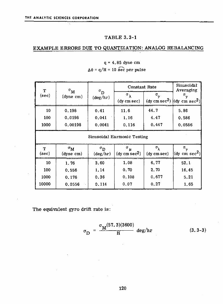
THE ANALYTIC SCIENCES CORPORATION
TABLE 3.3-1
EXAMPLE ERRORS DUE TO QUANTIZATION: ANALOG REBALANCING
q = 4.85 dyne cm
A6 = q/H = 10 sec per pulse
T(sec)
10
100
1000
cr,,M(dyne cm)
0.198
0.0198
0.00198
aD(deg/hr)
0.41
0.041
0.0041
Constant Rateax
(dy cm sec)
11.6
1.160.116
CTy ,(dy cm sec2)
44.7
4.47
0.447
SinusoidalAveraging
ay
(dy cm sec2)
5.86
0.586
0.0586
Sinusoidal Harmonic Testing
T(sec)
10
100
1000
10000
CTM(dyne cm)
1.76
0.556
0.176
0.0556
aD(deg/hr)
3.60
1.140.36
0.114
°» 0(dy cm sec2)
1.08
0.70
0.108
0.07
ffx(dy cm sec)
6.77
2.70
0.677
0.27
CTy(dy cm sec2)
52.1
16.45
5.21
1.65
The equivalent gyro drift rate is:
<rM(57. 3X3600)M'D H deg/hr (3.3-3)
120

THE ANALYTIC SCIENCES CORPORATION
The corresponding parameter estimation errors are:
W2 M
CT M
constant rate tests
(3.3-4)
(3.3-5)
CT = —9" CTM ^ sinusoidal averaging tests (3.3-6)W
For sinusoidal harmonic testing the rms errors in the Fourier coefficientestimates are:
(3.3-7)j
The values given in the lower part of Table 3.3-1 are based on theassumption that 10 samples per second are taken; that is, the sampleinterval h is 0.1 sec. The equivalent drift rate is again given byEq. (3.3-3). The corresponding parameter estimation errors are:
a(jL coW °M(3.3-8)
rX ~ W CTM(3.3-9)
(3.3-10)
121
THE ANALYTIC SCIENCES CORPORATION
R-1231
10
_ 0.1
010)
TJ
Q. b 0.01
0.001
0.0001
10
0.1
0.01
0.001
10 100 1000 1QOOO 10 100 1000 10,000Test Time,T(sec) Test Time,T(sec)
(a) Constant Rate and SinusoidalAverage Testing
Figure 3.3-2
(b) Sinusoidal Harmonic Testing
Effective Drift Rate Due to Quantization
Figure 3.3-2(a) plots CTD versus test time for four values of
quantization level, A 6. The two middle values (1 sec and 10 sec) are
comparable to single-pulse quantization levels for pulse rebalanced sen-
sors. The extreme values (80 sec and 0.04 sec) represent a range of
quantization levels obtainable from an analog rebalanced gyro. For
example if a voltage-to-frequency device with a full scale output rate of5000 counts/sec is used, the high quantization level would be necessary
for a maximum applied rate about the gyro input axis of 2 rad/sec,
which causes a torque of:
M = WH = 2
122

THE ANALYTIC SCIENCES CORPORATION
Therefore, the device must be scaled to make:
_ 2 x 10⁵ An.
qmax ~ -5000- = 40 dyne cm sec
and
™a^ = §: 2.06 x 105 = 80 secmax ti
The low quantization level would be possible for a test involving smalltorques only, such as an applied rate nominally about the gyro spin axis.If the maximum torque expected in this case is 100 dyne cm (see examplevalues in Section 3.5), then the device can be scaled to makeA0 - s- 0.04 sec. This points up a possible advantage in testing analogrebalanced sensors, as opposed to pulse rebalanced instruments. It maybe easier, in the analog case, to rescale the data processing electronicequipment to take good advantage of situations involving only low levels ofapplied output axis torque. By such a rescaling the quantization effectmay be reduced, with an attendant possibility of increased error due totorquer nonlinearity and signal generator noise.
For sinusoidal harmonic testing the error in the measurementof drift rate is proportional to the test motion frequency (co) and to thesquare root of the sample interval (h). This dependence is shown inFig. 3.3-2(b) where results are plotted for two values of the parameter,co //h, for each of the four quantization levels.
123

THE ANALYTIC SCIENCES CORPORATION
Pulse Rebalanced Sensors - It is highly desirable to test entire
strapdown instruments, including their rebalance electronics,, Since mostaccurate strapdown gyros and accelerometers are of the pulse rebalancedtype, the primary test output will be quantized,, The example calculationsand curves discussed above apply equally well to testing pulse rebalancedsensors in so far as the "error due to quantization" is concerned. How-ever, as discussed in Section 3.2.5, still larger errors associated withthe oscillatory behavior of nonlinear pulse rebalance loops may also occur.Consider, for example, pulse rebalance sensors in which the loop param-eters, test motion quantities and test time have the values given at the topof Table 3.3-2. The tabulated values for the characteristic frequency andamplitude of float angle oscillation and for the individual measurementerrors are obtained by application of the formulas given in Table 3»2r6.The values for torque estimation errors are obtained via Eqs, (3.2-41)and (3.2-42) for average torque and harmonic component estimates,respectively. These may be related to errors in estimating the X, y and/Literals via Eqs. (3.3-4, 5 and 6) and Eqs. (3.3-8, 9 and 10) just as inthe analog rebalanced case. The last column in Table 3. 3-2 is includedin order to relate the error due to loop dynamics to the error associatedwith the single pulse quantization level. The tabulated quantity is calledthe "effective loop quantization level" it is the quantization level whichwould cause the rms measurement error, a , already computed for a
"
given set of loop parameters, if the two had the same relationship pre-viously derived for the simple error due to quanitzation; namely:
CTG = q~«//6" . (3.3-11)
124

THE ANALYTIC SCIENCES CORPORATION
TABLE 3.3-2
EXAMPLE ERRORS DUE TO QUANTIZATION:PULSE REBALANCING
H = 10 dyne cm sec
C = 10 dyne cm sec2
I = 100 gm cmoo
T. = 0.001 sec
T. = 0.0001 sectg
ii =1 rad/sec1max 5M. = H to; =10 dyne cmtir "max '
T = 100 sec
h = 0.1 sec
uj = 2ir rad/sec
W = 0.26 rad/sec
Type ofRebalance
Loop
Binary
Ternary
r = 0.26
T) = 0.85
Time - Modu lation
T = 0.001P
T. = Tp/64
Frequency
(rad/sec)
3162
2688
6283
Amplitude
(mrad)
0.116
0.058
0.027
IndividualMeasurement
Error
(dyne cm sec)
38.5
16.6
17.2
[h = nT p ]
0.64
Estimation Error"M
(dyne cm)
AverageTorque
Estimate
0.385
0.166
0.172
0.0064
HarmonicComponent
Estimate
10.8
4.67
4.82
0.18
Effective LoopQuantization
LevelAjeff(sec)
194
84
87
3.2
Thus, converting q .. to angular form:
A9eff 76/H (3.3-12)
This quantity allows us to use the formulas and plots (Fig. 3.3-2) alreadydeveloped for the analog torquing case. Note that for the binary andternary loops as well as the time-modulation loop, whenh ^ nT , the effec-tive quantization level is considerably higher than a single pulse weight.
125

THE ANALYTIC SCIENCES CORPORATION
The lowest effective quantization level, by far, occurs in thisexample for the time-modulation rebalance case when the measurementinterval is controlled to be an integral number of pulse widths. Amongthe other three cases the ternary loop has the lowest effective quantiza-tion level, due to its low characteristic frequency of oscillation.
3.3.3 Time to Reach Equilibrium
This section treats the question of how long it takes forestimation errors to reach a state of equilibrium, defined largely by therelative magnitudes of measurement noise and process noise; by filteringdata taken over many cycles it is possible to reduce the effects ofuncorrelated random errors. The formulation of the first stage of thedata processing problem as one of linear estimation (see Appendix C) isuseful in indicating the length of time over which it makes sense to filterthe data; the state variables to be estimated in each single-axis vibrationtest are the seven Fourier coefficients.
Figure 3.3-3 is a conceptual plot showing how the estimationo j.i
error variance a. of the i state variable might change during the coursei 2
of a test, assuming the use of optimal filtering. The initial value a. (0) isa measure of the uncertainty regarding the variable prior to the start of
othe test. The final value a.(°°) represents an equilibrium condition that isreached after sufficient time, in which the information coming in by virtueof new measurements is balanced by the information being lost due toprocess noise; the final value is independent of the initial value. * The
2major reduction in CT. takes place while the curve tends to follow the
*This is only true if certain observability conditions are satisfied.
In the problem considered here these conditions are met.
126

THE ANALYTIC SCIENCES CORPORATION
g-1229
• Measurement Noise Only :
<r2( t ) = f (r)
• Complete Problem :
P = Q- -J-PHTHP
Figure 3.3-3 Estimation Error Variance Time History
dashed line labeled "measurement noise only." This dashed line cor-responds to a hypothetical, optimal filtering situation in which there is noprocess noise and the initial uncertainty is infinite. The dashed curve,therefore, depends on only one parameter, r, which characterizes themeasurement noise. It approaches zero asymptotically; by processingnoisy measurements of a deterministic quantity the estimation error ismade steadily smaller as time progresses.
A "solution time" or "settling time" t_ can be loosely definedo
as the time it takes the estimation error variance to get "close" to its
127

THE ANALYTIC SCIENCES CORPORATION
final valueo The significance of t is that a test should be allowed to con-stinue this long in order to get full benefit of the optimal filtering. A use-
ful measure of t can be taken as the time at which the dashed line crossessthe final value level (see Fig. 3.3-^3). This crossing point depends onmeasurement noise and process noise, but is independent of initial errors.
It can be found for any assumed set of measurement noise and process
noise statistics by methods developed in Appendix C.
An approximate formula for the settling time in (see Appendix C):
tg = /2^- (3.3-13)
where r and q.. characterize measurement noise and process noise,
respectively, as described in Section 3.2.4. Equation (3.3-13) is a com-panion to Eq. (3.2-70) which gives the final value of the estimation error.
Both are plotted parametrically in Fig. 3.2-8.
An alternate expression for the settling time, one which con-
siders the effect of correlated process noise components, is:
(3.3-14)
where c.. is a measure of correlation between two components of process13 thnoise, the j component being the one which dominates the problem.
Equation (3.3-14) is a companion to Eq. (3.2-71). Together they imply
that a high correlation between process noise components sometimes
reduces the final estimation error variance, at the same time increasing
the time needed to reach the more accurate level.
128

THE ANALYTIC SCIENCES CORPORATION
3.4 TEST DATA PROCESSING
The data processing function, for sinusoidal harmonic testing,can be defined in terms of the procedure pictured in Fig. 3.1-3 whichshows three data processing phases: Phase la accepts as input the scalar,periodically time-varying sensor output and generates the set of Fouriercoefficients for each single-axis test; in phase Ib the complete array ofestimated values of the Fourier coefficients for a sequence of six single-axis tests is processed to yield estimates of a complete set of basicparameter groups; in phase II the values of individual parameters arecomputed.
Phase la, in which raw test data is processed, directly influencesthe choice of laboratory data processing equipment (see Section 4.2). Threecandidate types of processing algorithms, Fourier analysis, least squaresestimation and Kalman filtering, are considered below. Phase Ib involvesthe estimation of the basic parameter groups from an array of redundantcoefficients. As a practical matter this phase may become a very simplecomputation based on a subset of "primary" coefficients, as discussed inSection 3.2.2, leaving the redundant information to be used as a cross-checkon the operation of the test sequence or as a means to indicate the existenceof previously unsuspected error torques. Alternatively, some form ofregression analysis may be used to develop an optimum fit to the entirearray of redundant data. The possible gain from such a procedure has notbeen investigated. Phase n, the simple algebraic calculation discussed inSection 2.4, requires no further study. This section will consider in detailthe form of the equations to be mechanized in order to perform phase la viathe three candidate algorithms.
129

THE ANALYTIC SCIENCES CORPORATION
3.4.1 Fourier Analysis
One obvious way to determine the coefficients of a trigonometric
series is by Fourier analysis. For two reasons the problem at hand maydiffer from a classical Fourier analysis problem. These are:
• Because of errors in measurements and test motionswe would like to process many cycles of data ratherthan just one.
• It may be necessary to deal with quantized rather thancontinuous data. This will certainly be true for apulse-rebalanced sensor since the data comes naturallyin quantized form. It may also be true if data from ananalog-rebalanced sensor is to be processed on a digitalcomputer.
The following equations are appropriate for computing Fouriercoefficients from a continuous output function e (t), taken over a timeinterval corresponding to m test motion cycles, where the test motionfrequency is co and the cycle period is T = 2ff/co:
The rebalance torque is assumed to be the continuous function:
Mtg(t) = Ktger(t) (3.4-1)
The applied torque is given by:
M = M. = B + S- sin cot + C., cos cota tg 1 1
+ S0 sin 2cot + C0 cos 2oot£i ft
+ S3 sin Scot + C3 cos 3cot (3.4-2)
130

THE ANALYTIC SCIENCES CORPORATION
The Fourier coefficient estimates are:
K,j er(t)dt (3.4-3)
o
2K mT
n T rS = ~ e ( t ) sin no* dt (3.4-4)
2K rCn = InT \ er(t) COS nwt * (3.4-5)
o
where n = 1, 2 and 3.
Equations (3.4-3), (3.4-4) and (3.4-5) reduce to the classical Fourieranalysis equations when m is unity. These equations can be mechanizeddirectly on an analog computer for a sensor which is analog-rebalanced, in
which case e (t) is produced as an analog signal.
For the pulse rebalanced case, two sets of exact equations which
generate the Fourier coefficients corresponding to the square-wave-type
torque generator output are developed in Appendix D. For the binary andternary^ pulse schemes the equations for the sine and cosine coefficients
are:
km-1
i=0S = y] M. [(l-cos ncoh)cos nwhi + sin ncoh sin nwhi] (304-6)
131

THE ANALYTIC SCIENCES CORPORATION
C = —— y M. [(l-cos ncoh)sin ncohi - sin ncoh cos ncohi] (3.4-7)n
km-1
i=0
where:
n = 1, 2 and 3
h = pulse width
w = test motion frequency
m = number of cycles processed
k = number of pulse widths per cycle (2ir/uih)
and M. defines the torque level of the i pulse according to:
M positive torque levelM. = 0 zero torque level
M negative torque level
The bias Fourier coefficient is proportional to the net pulse count,, That is:
km-1
£i=0
B = £ Mi
For the time-modulated pulse torquing scheme the equations forthe sine and cosine coefficients are :
132

THE ANALYTIC SCIENCES CORPORATION
km-1M
n ream- (2 cos nco4. - cos ncoh) cos ncohi
+ (2 sin nco L- sin ncoh) sin ncohi | (3.4-9)•1km-1
Cn =M 12 cos nco 4. - cos ncoh) sin ncohi
i=0
+ (2sin nco &.- sin ncoh) cos ncohi | (3.4-10)j
where n, m and k are defined as above; M is the absolute value of the torque
level; H. is the width of the positive torque pulse in the i interval; each
interval has both positive and negative pulses and has the total width, h.
The bias Fourier coefficient is given by:
km-1
B = Mmk
i=0h- (3.4-11)
Since h is very small compared to one test motion period, and since
L is less than h, we can employ the following small angle approximations:
cos ncoh = cos nco L = 1
sin ncoh = ncoh
cos nco L = nco L
(3.4-12)
133

THE ANALYTIC SCIENCES CORPORATION
The equations given above reduce to the following set of unified, approximate
expressions:
km-1
£i=0
Sn ~ In^r ^ bisin (n(ohi) (3.4-14)
km-1
i=0
km-1r ~^.x Y** D- cos (ncohi) (3.4-15)
n ~ mT 2-, 1
i=0
where we have used T = 2ir/u and the definitions:
b. = sgn (Mj) (binary and ternary) (3.4-16)
a. - h/2b. = 1
/9—(pulse-width modulation) (3.4-17)i \\./ ft
Note that Eqs. (3.4-13), (3..4-14) and (3.4-15) look like discrete approxi-mations to Eqs. (3.4-3), (3 = 4-4) and (3.4-5) for the analog-rebalanced case.
In both cases, the sensor output (the continuous signal, e , or the sequence,
is multiplied by the "weighting" functions (sin nojt or sin nwhi and
cos nojt or cos ncohi) and integrated or summed to produce the desiredFourier coefficients (S^ and Cn).
134

THE ANALYTIC SCIENCES CORPORATION
3.4.2 Least Squares Estimation
A least squares estimation procedure is outlined in Section 3.2.4.
This procedure applies to the case in which the data is a sequence of integers
(z1, z0,... z.), each representing the integral of torque over a specified1 z ]interval of time. The least squares estimate of the vector:
x = (3.4-18)
of harmonic coefficients is given by:
-1x = (HTH) HT (3.4-19)
where the measurement matrix, H, is:
H = -1W
(3.4-20)
fi gi Pj 0)
135

THE ANALYTIC SCIENCES CORPORATION
Where:
f. = - cos cohi + cos coh(i-l)
= sin tohi - sin coh(i-l)
p. = - TJ cos 2u>hi + T> cos 2coh(i-l)1 Lt £l
CL. = sin 2whi - sin 2cjh(i-l) (3.4-21)
Processing data by means of Eq. (3.4-19) is essentially similar
to Fourier analysis, in that we are multiplying a sequence of measurements
by a set of periodically varying weighting functions (the elements of H^) to
obtain estimates of the various harmonic coefficients.
The computation can be simplified in practice if an integral
number (say k) of data intervals, h, occur in one test motion period. In
this case the elements of each column of H are cyclically repeating:
f = f = fi i+k i+2k
gi " gi+k
etc. (3.4-22)
These sequences of repeating elements multiply the sequence of measure-
ments:
zi+k' zi+2k' ' ' *
136

THE ANALYTIC SCIENCES CORPORATION
Therefore, we can add up the raw pulse count data in k sections. Forexample, define the k sums:
m-1Zi = E z ( i = 1>2 , . . .k) (3,4-23)
4=0
where m = j/k, the number of test cycles. Then:
H?" , z. = I? „ Z. (3.4-24)kmx4 —km kx4 k
~Twhere H, . is the single- cycle measurement matrix, which repeats itselfTm times as a partition of H , as follows:
^n I rri I rp | rp I | ^^^^^ 1
H = H ;H |H i JH (3.4-25)L i i i i J
When this simplified procedure is used, the on-line (real-time) data pro-cessing function involves Eq. (3.4-23) only, generating the k outputs,Z.. through Z,.
3.4.3 Kalman Filtering
In Appendix C the phase la data processing problem is formulatedas a problem in linear estimation for which the Kalman filter is an optimalsolution. This formulation is a useful analytical device for determining theeffects of random process noise and measurement noise on the test accuracy
137

THE ANALYTIC SCIENCES CORPORATION
(Section 3.2-6) and the useful test duration (Section 3.3). This section
discusses the advisability of using a Kalman filtering algorithm in
processing real test data — the form of the equations to be mechanized and
the advantage there might be in using Kalman filtering in preference to
Fourier analysis.
The following Kalman filter equations are appropriate for the
continuous (analog rebalanced) case:
x(t) = K(t) [z(t) - H(t) x(t)] (3.4-26)
K(t) = ^P(t)HT(t) (3.4-27)
P(t) = Q-^P(t)HT(t)H(t)P(t) (3.4-28)
where x is the optimal estimate of the seven-state (five, if third harmonics
are ignored) state vector x composed of the set of Fourier coefficients, z
is the time-varying scalar measurement (the output of the sensor) and K isthe Kalman filter gain matrix which in this case is a 7 x 1 column vector.
H is the measurement matrix (in this case a 1 x 7 row vector) with
periodically time-varying elements:
H(t) = (1, sin cot, cos tot, sin 2tot, cos 2cot, sin 2cot, cos 3cot)(3.4-29)
and P is the covariance matrix of the estimation error:
P = ( x - x ) (x-x)T (3.4-30)
138

THE ANALYTIC SCIENCES CORPORATION
The constant scalar r and the constant matrix Q characterize themeasurement noise and process noise, respectively, as discussed inSection 3.2-6. For any given test set-up, Eq. (3.4-28) could be integratedin advance and the result could be substituted into Eq. (3.4-27) to producea gain matrix with time-varying elements. This function could then be usedin real time in Eq. (3.4-26) to process actual test data, z(t). If the actualtest is generated in digital form, an alternate expression, based on thediscrete form of the Kalman filter, may be used.
Appendix C demonstrates that after some time has elapsed fromthe start of a test, the Kalman filtering equations above become approxi-mately equivalent to the Fourier analysis procedure in which successivecycles of processed data are averaged together. Therefore, the onlyobvious difference in the Kalman filter procedure involves the way the datafrom the first few cycles are processed. The filter estimates in these earlycycles should be superior because all available information, including priorestimates, is being used in an optimal way. Since certain sensor parametersshould be known accurately prior to the test this advantage may be quitesignificant, especially if the data processing equipment imposes severelimits on the amount of data which can be handled from a given test.
There is another potential advantage of the Kalman filteringapproach which can be significant if some of the sensor parameters undergosignificant changes during the course of a particular vibration test. Theformulation of the problem can be expanded to take account of such changes(with, for example, a random-walk model) and the changes can be "tracked"during the test, with the result that the optimal estimates produced aresignificantly more accurate than those generated by Fourier analysis orsimple least squares estimation. It is expected, however, that the
139
THE ANALYTIC SCIENCES CORPORATION
parameters under consideration will not change fast enough to make this astrong consideration in choosing a data processing scheme.
In summary, there are two potential advantages of the Kalmanfiltering approach — the inclusion of prior estimates and the possibility of
tracking parameter changes, but more study is required before a definiterecommendation concerning its use can be made.
3. 5 EXAMPLE CALCULATIONS
This section presents the results of illustrative numerical cal-culations corresponding to an analog rebalanced single-degree-of-freedomgyro undergoing angular motion tests. The six recommended test motionaxes and all three types of testing are included. The calculations includetest errors, typical torque levels, and the variation of torque levels withtest motion quantities. The test errors are based on the formulas developedin Section 3.2. The error calculations provide a quantitative accuracycomparison of the three types of single axis testing, augmenting the dis-cussion at the end of Section 3.2.1.
3.5.1 Torque Levels
Table 3.5-1 lists the values of the parameter groups used in theexample calculations. Table 3.5-2 lists the jj, X and y terms corresponding
to the given gyro parameters, the assumed test motion quantities W andco (the same amplitude and frequency are used for all six test axes), and thetorque amplitudes (M .. M and M ) which occur during sinusoidal testing.Note that M. is the same as the value, XW, corresponding to a constant rate
A.
140

THE ANALYTIC SCIENCES CORPORATION
TABLE 3. 5-1
ASSUMED GYRO PARAMETER VALUES
kl=ttsIoo'IoiS
oo = -100 gm cm2
,2= gm cmg
k. = H = 105 gm cm2/sec
kK = a H = 5 gm cm2/secD S
k« = -fl H = 5 gm cm2/sec'
(a a - 10 sec)S
(S0 =-10 sec)
Vg
= 10 gm cm2
g
=-50 gm cm2
= 1 gm cm2
o
A14
= -H/K(I -i..^ -I..) =-0.05 gm cm2 secy ss ii/ /
0.1 gm cm2 sec2
5 x 10~5 gm cm2 sec2
oo ss - I . . ) =-ii/
K = 10° dyne cm/radian(Iss-Iii) = 50 gm cm2
141

THE ANALYTIC SCIENCES CORPORATION
TABLE 3. 5-2
ILLUSTRATIVE TORQUE LEVELS
Sinusoidal Test Motion: W = 1 rad/sec, w = 6.28 rad/sec (1 Hz)
Test
Axis
o
s
i
o/s
i/o
i/«
p
(dyne cm sec )
kj =-100
k3 = 1
k1 = l
^(VSH-5
k!3 ' 0'1
^(VaH-5
71( 3) = '•««
M^nuW
(dyne cm)
-628.0
6.28
6.28
-449.0
0.16
-449.0
8.89
X
(dyne cm sec)
V 5
kg = 5
TflVeV7-07
^(V*B) "">-™>
7f(vk6)-70-TOO
M X = X W(dyne cm)
5.0
5.0
105
7.07
70,700
70,700
y
(dyne cm sec )
kg = 10
-k , - l
k7 = l
j(-k' + k8+kll)= *
Kk' + k8+k9) = 5
I kio =-25
M^lw2
(dyne cm)
5.0
0.5
0.5
3.0
2.5
-12.5
test at the rate, W, and M is one half the value, ^W , corresponding to aconstant rate test at the rate, W. The larger torque levels occur as M
A
when the test axis is i, i/o or i/s; these involve gyroscopic terms,The medium-sized levels occur as M when the test axis is o, o/s or i/o;these involve output axis inertia terms, I to . All other terms areoo orelatively small. The M terms, which are not included in the table, are
Pextremely small. For example:
M =8/2
= 0.013 dyne cm
142

THE ANALYTIC SCIENCES CORPORATION
Similarly, the \i term involving k... is:
M = —J— k , ooW3 = 0.000028 dyne cm8/2" 14
The variation of test torque levels with the magnitude of the appliedtest motion quantities (W and co) is illustrated in Figs, 3. 5-1 and 3. 5-2. Thetorque levels corresponding to each basic parameter group which contributestorque in the o, s, and i axis tests are plotted versus W in Fig. 3.5-1 and theleft hand side of Fig. 3. 5-2. The right hand side of Fig. 3, 5-2 plots thetorques produced in the o/s, i/o and i/s axis tests by those parameter groups(kq, k10, k... and k..-) which do not contribute in the first three tests. Thecontributions of the parameters already covered in the previous plots are notshown. For example, k. produces large torques in both the i/o and i/saxis cases; their magnitudes are 1/^2 times the value shown (labeledfor the i axis test.
The M levels (M^.^. k«>) are linear in both W and to. The Mlevels (Mfc. ^ ^ ) are linear in W and independent of to. The M levels
(Mk7,ka ka kin ki i ) are proprotional to W and independent of co. TheM term, Mi,1Q, is proportional to W2 and linear in to.
fJL lO
It is worth noting that for a fixed amplitude, A, of angularexcursions in a sinusoidal test, all of these quantities vary with frequency.Thus, if:
9test = Asin "* (3.5-1)
143
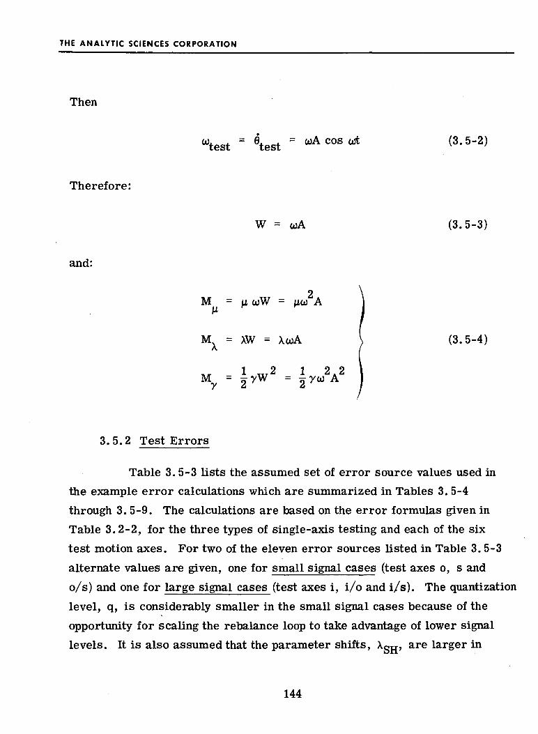
THE ANALYTIC SCIENCES CORPORATION
Then
"test = 9test = <°A COS °* (3.5-2)
Therefore:
W = coA (3.5-3)
and:
M = u, coW = uw A
= XW = XooA
1 ...2 1 2.2M = VW = r<° A
(3.5-4)
3.5.2 Test Errors
Table 3.5-3 lists the assumed set of error source values used inthe example error calculations which are summarized in Tables 3. 5-4through 3. 5-9. The calculations are based on the error formulas given inTable 3.2-2, for the three types of single-axis testing and each of the sixtest motion axes. For two of the eleven error sources listed in Table 3.5-3alternate values are given, one for small signal cases (test axes o, s ando/s) and one for large signal cases (test axes i, i/o and i/s). The quantizationlevel, q, is considerably smaller in the small signal cases because of theopportunity for scaling the rebalance loop to take advantage of lower signallevels. It is also assumed that the parameter shifts, X, are larger in
144

THE ANALYTIC SCIENCES CORPORATION
R-1233
10
10
104
10
io1)
0.1
0.01
MOTION ABOUT
OUTPUT AXIS
MOTION ABOUT
SPIN AXIS
0.01 0.1 1
W(rad/sec)
0.01 0.1 1W( rod/sec)
Figure 3.5-1 Variation of Torque Levels With Test MotionAmplitude and Frequency: o and s Test Axes
145

THE ANALYTIC SCIENCES CORPORATION
H-»34
10
10
104
io
u
0)c
'0
10
O.I
0.01
MOTION ABOUT
INPUT AXIS
0.01 0.1
W( rod/sec)
"i/o" TEST:k,
"i/s" TEST: k,0
0.01 0.1 1
W (rod/sec)
Figure 3.5-2 Variation of Torque Levels With Test MotionAmplitude and Frequency:!, o/s, i/o and i/sTest Axes
146
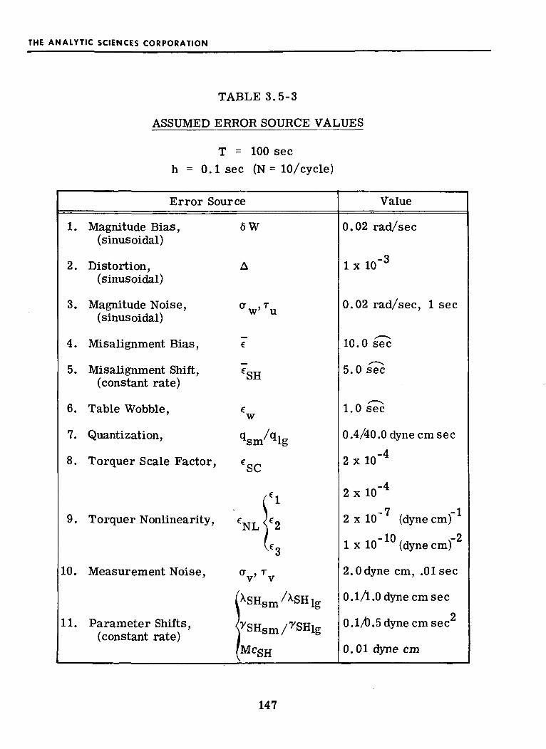
THE ANALYTIC SCIENCES CORPORATION
TABLE 3.5-3
ASSUMED ERROR SOURCE VALUES
T = 100 sech = 0.1 sec (N = 10/cycle)
Error Source Value
1. Magnitude Bias,(sinusoidal)
2. Distortion,(sinusoidal)
3. Magnitude Noise,(sinusoidal)
4. Misalignment Bias,
5. Misalignment Shift,(constant rate)
6. Table Wobble,
7. Quantization,
9. Torquer Nonlinearity,
10. Measurement Noise,
11. Parameter Shifts,(constant rate)
6W
CTWTu
SH
w
qsm/qlg
8. Torquer Scale Factor, e noU
CNL <<2
CT , TV V
ASH i
McSH
0.02 rad/sec
1 x 10"3
0.02 rad/sec, 1 sec
10.0 sec
5.0 sec
1.0 sec
0.4/40.0 dyne cm sec
-42x 10
2 x 10"4
-7 -12 x 10 (dyne cm)
1 x 10 ~ (dyne cm)~
2.0dyne cm, .01 sec
0.1/1.0 dyne cm secn
0.1/t).5dyne cm sec
0.01 dyne cm
147

THE ANALYTIC SCIENCES CORPORATION
TABLE 3.5-4
EXAMPLE ERROR SUMMARY: o TEST AXIS
9 2= 100 dyne cm sec^ = 5 dyne cm sec = dyne cm sec
1. Magnitude Bias 6W
2. Distortion A
3. Magnitude Noise CTW
4. Misalignment Bias ?
5. Misalignment Shift ?_„on
6. Table Wobble, cw
7. Quantization q
8. Torquer Scale Factor *„_
9. Torquer Nonlinearity ej
CNL '2e3
10. Measurement Noise a
11. Parameter Shifts X__Oil
ySHMCSH
Total (RSS) aCTXay
Constant Rate
X
0
...
0
5.0
2.5
0.5
0.016
0.001
0.00001
0.79
0.142
5.67
y
0
—
0
0
1.25
0.25
0.008
0.002
0.0001
0.40
0.079
1.34
SinusoidalAveraging
y
0.2
0
0.67
0
—
0
0.003
0.002
0.002
0.16
—
0.72
Sinusoidal Harmonics
\i
2.0
0
0.42
0
—
0
0.007
0.02
0.104
0.013
—
2.05
X
0.1
0
0.24
5.0
—
0
0.046
0.001
0
0.079
—
5.01
V
0.2
1.26
0.67
0
—
0
0.092
0.002
0.001
0.16
...
1.45
148

THE ANALYTIC SCIENCES CORPORATION
TABLE 3.5-5
EXAMPLE ERROR SUMMARY: s TEST AXIS
k X = k v = k3 g 6 ' 21 dyne cm sec = 5 dyne cm sec = 1 dyne cm sec
1. Magnitude Bias 6W
2. Distortion A
3. Magnitude Noise <j
4. Misalignment Bias f
5. Misalignment Shift rgH
6. Table Wobble «w
7. Quantization q
8. Torquer Scale Factor egc
9. Torquer Nonlinearity f j
€NL e2€3
10. Measurement Noise a
11. Parameter Shifts (XSH )
IvSH (
(MCSH)
Total (RSS) Olt
"ACTy
Constant Bate
X
0
...
0
5.0
2.5
0.5
0.016
0.001
0.000001
0.79
0.142
5.67
7
0
...
0
0
1.25
0.25
0.008
0.0002
0.00001
0.40
0.079
1.34
SinusoidalAveraging
y
0.02
0
0.21
0
—
0
0.003
0.0002
0
0.16
...
0.21
Sinusoidal Harmonics
It
0.02
0
0.04
0
—
0
0.007
0.0002
0
0.013
—
0.045
X
0.1
0
0.24
5.0
—
0
0.046
0.001
0
0.079
...
5.01
y
0.02
0
0.21
0
—
0
0.092
0. 0002
0
0.16
—
0.23
149

THE ANALYTIC SCIENCES CORPORATION
TABLE 3.5-6
EXAMPLE ERROR SUMMARY: i TEST AXIS
i = k X = k. y = k,2 B 2= 1 dyne cm sec = 10D dyne cm sec = 1 dyne cm sec
1. Magnitude Bias 6W
2. Distortion A
3. Magnitude Noise aw
4. Misalignment Bias ~e
5. Misalignment Shift Tgjj
6. Table Wobble *w
7. Quantization q
8. Torquer Scale Factor fg£
9. Torquer Nonlinearity cj}eNL e2/
es)10. Measurement Noise ay
11. Parameter Shifts XSH
?SHMCSH
Total (RSS) a
CTXcry
Constant Rate
X
0
...
0
0
0
0
1.63
20.0
3.0
0.79
1.01
20.3
y
0
...
0
0
0
0
0.815
0.0002
30.0
0.40
0.50
30.0
SinusoidalAveraging
y
0.02
0
0.21
0
—
0
0.326
0.0002
25.5
0.16
...
25.5
Sinusoidal Harmonics
V-
0.02
0
0.04
0
—
0
0.728
0.0002
0
0.013
—
0.73
X
2000
0
33.5
0
...
0
4.58
20.0
16.0
0.079
...
2000
y
0.02
200
0.21
0
—
0
9.16
0.0002
17.0
0.16
...
201
150
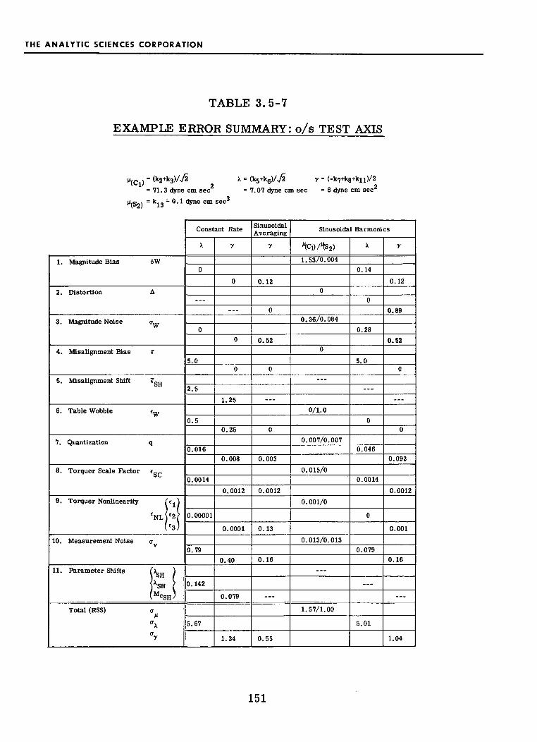
THE ANALYTIC SCIENCES CORPORATION
TABLE 3.5-7
EXAMPLE ERROR SUMMARY: o/s TEST AXIS
X = <k5+k6)/,/2 y = (-k7+k8+k11)/2
= 71.3 dyne cm sec = 7.07 dyne cm sec = 6 dyne cm sec2
= 1r =O1 /hmo r*m cor*''
1. Magnitude Bias 6W
2. Distortion A
3. Magnitude Noise CTW
4. Misalignment Bias e
5. Misalignment Shift ?gH
6. Table Wobble ew
7. Quantization q
8. Torquer Scale Factor e__,at*
9. Torquer Nonlinearity e-
eNL (2e3
10. Measurement Noise a
11. Parameter Shifts X,,.,
XSHMCSH
Total (RSS) a
"\
°y
Constant Rate
X
0
—
0
5.0
2.5
0.5
0.016
0.0014
0.00001
0.79
0.142
5.67
y
0
—
0
0
1.25
0.25
0.008
0.0012
0.0001
0.40
0.079
1.34
SinusoidalAveraging
y
0.12
0
0.52
0
...
0
0.003
0.0012
0.13
0.16
...
0.55
Sinusoidal Harmonics
tCi)/1?32)
1.53/0.004
0
0.36/0.084
0
...
0/1,0
0.007/0.007
0.015/0
0.001/0
0.013/0.013
—
1.57/1.00
X
0.14
0
0.28
5.0
...
0
0.046
0.0014
0
0.079
—
5.01
y
0.12
0.89
0.52
0
...
0
0.092
0.0012
0.001
0.16
—
1.04
151
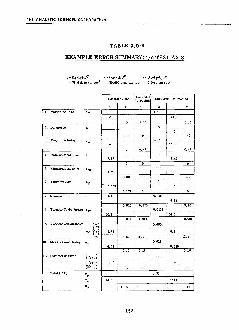
THE ANALYTIC SCIENCES CORPORATION
TABLE 3.5-8
EXAMPLE ERROR SUMMARY: i/o TEST AXIS
ft = (k!+k2)/,/2 X = (k4+k5)/,/2 y = (k7+k8+kg)/2
= 71. 5 dyne cm sec = 70,000 dyne cm sec = 5 dyne cm sec^
1. Magnitude Bias 6W
2. Distortion A
3. Magnitude Noise cr...w
4. Misalignment Bias f
5. Misalignment Shift ?gH
6. Table Wobble *w
7. Quantization q
8. Torquer Scale Factor c__oO
9. Torquer Nonlinearity f -
€NL £2e3
10. Measurement Noise a
11. Parameter Shifts XOIIoilySH
MCSH
Total (RSS) a
°\
°7
Constant Rate
X
0
...
0
3.53
1.77
0.353
1.63
14.1
1.35
0.79
1.01
14.8
V
0
—
0
0
0.88
O!l77
0.815
0.001
13.53
0.40
0.50
13.6
SinusoidalAveraging
y
0.10
0
0.47
0
—
0
0.326
0.001
18.1
0.16
...
18.1
Sinusoidal Harmonics
M
1.53
0
0.36
0
- —
0
0.728
0.0153
0.0006
0.013
...
1.73
X
1414
0
28.2
3.53
— -
0
4.58
14.1
6.9
0.079
1414
y
0.10
142
0.47
0
0
9.16
0.001
12.1
0.16
.--
143
152

THE ANALYTIC SCIENCES CORPORATION
TABLE 3.5-9
EXAMPLE ERROR SUMMARY: i/s TEST AXIS
H = (k1+k3)/y2 X = (k^kgJA/Z y = k10/22 ?= 1.414 dyne cm sec = 70, 7000 dyne cm sec = 25 dyne cm sec
1. Magnitude Bias 6W
2. Distortion A
3. Magnitude Noise CTW
4. Misalignment Bias e
5. Misalignment Shift Tgjj
6. Table Wobble « w
7. Quantization q
8. Torquer Scale Factor egg
9. Torquer Nonlinearity cj
^L C2e3
10. Measurement Noise a
11. Parameter Shifts XgH
rSHMCSH
Total (RSS) a
CTXCTy
Constant Rate
X
0
—
0
3.53
1.77
0.353
1.63
14.1
1.35
0.79
1.01
14.9
V
0
—
0
0
0.88
0.177
0.815
0.005
13.53
0.40
0.50
13.6
SinusoidalAveraging
y
0.50
0
1.06
0
...
0
0.326
0.005
18.0
0.16
...
18.0
Sinusoidal Harmonics
M
0.028
0
0.05
0
0
0.728
0.0003
0
0.013
—
0.73
X
1414
0
28.2
3.53
—
0
4.58
14.1
6.9
0.079
...
1414
y
0.50
141
1.06
0
0
9.16
0.005
12.0
0.16
...
142
153

THE ANALYTIC SCIENCES CORPORATION
in the large signal cases; these shifts represent very small percentage
changes in very large quantities (see Table 3. 5-2). The assumed testmotions are:
W = 2 rad/sec
W2 = 0.1 rad/secconstant rate tests
W = 1 rad/sec
W = 2n rad/secsinusoidal tests
The calculation of the time-dependent errors is based on the test time:
T = 100 sec.
In each column of Tablse 3.5-4 through 3.5-9 the values in the third andtenth rows have been compared, and the smaller of the two dropped, beforecombining errors in RSS fashion to calculate the overall one-sigmaestimation errors, a , cr. or a , given at the bottom of the column. (See
H A *Xthe discussion in Section 3.2.1.) In each column the one or two largestcontributions to the overall error are printed in red.
Table 3.5-10 summarizes selected results from the six precedingtables. For each of the parameter groups, k^ through kj. and k^, the testaxis which appears best suited for determining that parameter group isshown in Table 3.5-10, along with the corresponding one-sigma estimationerror. For example, k» = y for spin axis tests and input axis tests, but theone-sigma estimation error, a , is much smaller in the former case(compare Tables 3. 5-5 and 3.5-6), so the value for the spin axis test is
154
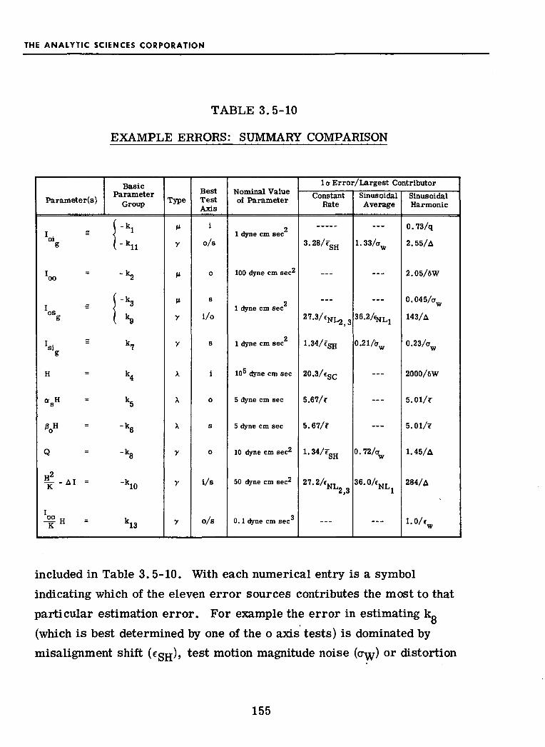
THE ANALYTIC SCIENCES CORPORATION
TABLE 3.5-10
EXAMPLE ERRORS: SUMMARY COMPARISON
Basic. . Parameter
Parameter(s) Group
'oi* " 1 - k!iXoo = " ^
ose / k_g ( "9
Isig S
H = k4
ru H — VOf n ~ KCs 5
V = -k6
Q = ^
H2
Tc-* ' = -kio
'"O H - k~TC H K13
Type
y
M
y
y
X
X
X
y
y
y
BestTestAxis
i
o/s
o
s
i/o
s
i
o
s
o
i/s
o/s
Nominal Valueof Parameter
21 dyne cm sec
100 dyne cm sec2
21 dyne cm sec
21 dyne cm sec
105 dyne cm sec
5 dyne cm sec
5 dyne cm sec
10 dyne cm sec^
50 dyne cm sec^
0
0. 1 dyne cm sec
1 o Error/Largest ContributorConstant
Rate
3.28/c-SH
—
27'3/fNL2)3
1.34/fgH
20.3/esc
5.67/f
5.67/e
1.34/FSH
27. 2ANL2,3
—
SinusoidalAverage
1.3S/ffw
---
0.21/irw
---
„_
...
o.«/v
"•«V,
—
SinusoidalHarmonic
0.73/q
2.55/A
2.05/6W
0.045/aw
143/A
0.23/aw
2000/6W
5.01/r
5.01/c
1.45/A
284/A
'•"«.
included in Table 3. 5-10. With each numerical entry is a symbolindicating which of the eleven error sources contributes the most to thatparticular estimation error. For example the error in estimating kg
(which is best determined by one of the o axis tests) is dominated bymisalignment shift ( f ) , test motion magnitude noise (ayy) or distortion
155

THE ANALYTIC SCIENCES CORPORATION
(A), depending on which of the three types of test is used (refer back toTable 3. 5-4). The parameter groups, k.g and k. ., are not included in the
example error calculations because of their extremely small size, (see
Section 3.5-1).
With three exceptions (kg,kjo an(* ^ll) *ne one-sigma estimationerrors given in Table 3. 5-10 are simply the appropriate RSS values(a ,CT ,cr ) given at the bottom of Tables 3. 5-4 through 3. 5-9. Forexample, the value 0. 73 for the k.. estimation error comes from the valuefor a given at the bottom of Table 3. 5-6. However, kQ and k1 n appear only
LJL */ J. A
in combination with k- and k0 in the definition of y in the o/s and i/o testI O
axis cases, respectively. Therefore, k_ and k~ must be estimated first(using s and o axis tests) and subtracted from the current estimate of yasfollows :
k9 = 2VsA A
A A
= 2y / -y -y (3.5-7)'o/s ' s o
and
A A
= 2Vo + k7 - k8
A A A
= 2y. i +y - y (3.5-8)'i/o s o
156

THE ANALYTIC SCIENCES CORPORATION
The values shown in Table 3.5-10 for cri, and a\. are computed from
(3.5-9)
and
°k11A
2 u. 2+ CT + CT
o J
1/2(3.5-10)
In a similar manner:
cr,1/2
(3.5-11)
Table 3. 5-10 is arranged to illustrate the relative difficulty indetermining the various individual parameters (I . , I , etc) using the
Olnr OO
several types of single axis testing. For the error source values assumedhere, it may be observed that:
The cross product of inertia, Ioig, may be determined askj by sinusoidal harmonic testing about the input axis oras k;Q by any of the three types of testing about the o/saxis. The smallest of the estimation errors shown cor-responds to the first method (even though it is a largesignal case — the /n term is not affected by distortion,nonlinearity and magnitude bias the way the X and y termsare). However, all four values are of the same order ofmagnitude and each has a different largest contributor, sothe relative estimation errors are very sensitive to theerror sources.
157

THE ANALYTIC SCIENCES CORPORATION
The cross product of inertia, IOSK> may also be determinedin any one of four ways, as k3 (one way) or as kg (threeways). In this case there is a clear preference for findingk3 using sinusoidal harmonic testing (about the s axis),since nonlinearity and distortion have major effects on thedetermination of kg, which requires the large signal testaxis i/o.
The cross product of inertia, Isiff> maY be measured in any
one of three ways, with angular motion about the spin axis.Sinusoidal testing (averaging or harmonic) appearssignificantly more accurate than constant rate testing,although this conclusion depends on the values of the dominanterror sources, which are different for the two types of testing.
The output axis inertia, Ioo, appears as a \i term only, andmeasuring its effect requires the use of sinusoidal harmonictesting about the output axis. The dominant error sourceappears to be uncertainty in the knowledge of the appliedtest motion amplitude.
Measuring the wheel momentum, H, involves rotation aboutthe input axis, using a constant rate on a sinusoidal oscillation.The former is much preferred because the applied constantrate magnitude will be known more accurately than theamplitude of the oscillation.
The misalignments, as and 0O, of the sensitive axis of thegyro may be determined using constant rate or sinusoidalharmonic testing about the output and spin axes, respectively.The two types of tests appear to be approximately equal inaccuracy since both are dominated by the bias misalignment,c, of the test axis. However, if the procedure of reversingthe sensor on the table top and repeating each run is used,the bias misalignment effect may be largely eliminated. Inthat case different error sources become dominant in thetwo cases: misalignment shift for constant rate testing, andtest motion magnitude noise for sinusoidal harmonic testing.
The experimentally observed error term, Q, may bemeasured in any of the three ways, rotating about the outputaxis. The smallest estimation error shown in that cor-responding to sinusoidal averaging, although all three areroughly equal and each has a different largest contributor.
158

THE ANALYTIC SCIENCES CORPORATION
• The kjQ parameter group, H2/K-(Iss-Iii), may be measuredin any of three ways, rotating about the i/s axis (a largesignal case). Sinusoidal harmonic testing appears uselessdue to the large distortion effect. The estimation errors inconstant rate testing and sinusoidal averaging are dominatedby torquer nonlinearity, the odd nonlinearities, €2 and €3,in the former case and the even nonlinearity, ej_, in thelatter case. In actual practice since kjo is made up of"desired" or nominal gyro parameters, its value should beknown a priori more accurately than it can be determined byeither of these i/s axis tests. This suggests that the reasonfor running such tests may be to compare the indicated and apriori values of kjo an^ to employ the differences asmeasures of the two types of torquer nonlinearity. Theresulting measures of the nonlinear terms can then be usedto correct the estimates of kg as obtained in the i/o axistests. A set of input axis tests can also be run to obtainanother measure of the nonlinearities.
• The ki3 parameter group, IOOH/K, appears only as a \JLterm and only in the o/s axis sinusoidal harmonic test.Based on the assumed error source values and parametervalues the one-sigma estimation error is considerablylarger than the nominal value of ki3. The dominant errorsource is table wobble, %. Removal of its contributionreduces the overall error to 0.085 dyne cm sec^. Sincethe value of kis is well known a priori, an attempt tomeasure it in this way might be useful in verifying theaccuracy of a sinusoidal harmonic testing set-up.
In summary, the reasons for considering the use of sinusoidalharmonic testing are that it provides the only way to measure the effect ofI , the best way to estimate Ios and reasonably good redundant estimatesof several other gyro parameters in the small signal cases (test motionaxes o, s, and o/s). Sinusoidal averaging does not yield anything that is notprovided by constant rate testing, but appears to have better accuracy in
several cases.
159

THE ANALYTIC SCIENCES CORPORATION
The example calculations summarized above are based on the
error formulas developed in Section 3.2 and tabulated in Table 3.2-2.In this case the formulas are used to compute parameter estimationaccuracies for an assumed set of error source values and test motionquantities. The same formulas can also be used, in a less straight-forward fashion, to generate test equipment performance specifications for
given desired estimation accuracies (see examples in Chapter 4).
Chapter Summary — The information which may be extractedfrom single-axis vibration tests and constant motion tests is identified.The effects of various test error sources, such as test machinery errorsand measurement errors, on the accuracy of estimating various observablequantities are analyzed. The different types of tests are compared on thebasis of observable quantities, data redundancy, number of test runs
required, data processing difficulty and accuracy.
All basic parameter groups can theoretically be computed fromthe observable quantities obtained in a sequence of six angular and six linearsingle-axis vibration tests if the harmonic content of the periodic appliedtorque function is extracted. The six test vibration axes should be orientedparallel to the three principal sensor axes--input, output and spin (orpendulum)--and to the three axes lying midway between pairs of principalaxes. The full array of observable quantities from a complete test sequenceprovides a considerable amount of redundant data which "overspecifies" the
basic parameter groups„
160

THE ANALYTIC SCIENCES CORPORATION
A sequence of sinusoidal vibration tests in which only averagetorque measurements are made yields only the parameter groups which givetorques proportional to the square of angular rate or acceleration, and noredundant data. However, the data processing requirements for determiningaverage torque are considerably simpler than for extracting harmonic terms.Extraction of certain harmonic terms provides redundant measurements ofthese parameter groups but they are generally less accurate than themeasurements based on average torque.
All of the parameter groups except those which generate torquesproportional to angular accelerations can theoretically be computed fromthe data produced in a sequence of constant motion tests. More test runs arerequired since two or more different magnitudes must be used for each testaxis in order to separate the effects of various parameter groups. The dataprocessing function is the same as in sinusoidal averaging, and thereforesimple. Parameter estimation errors are more affected by some test errorsources and less affected by others, as compared to sinusoidal testing.
The data processing function for sinusoidal harmonic testing con-sists of three phases. The first phase, in which harmonics are extractedfrom the sensor output data for each run, directly influences the choice oflaboratory data processing equipment. Three candidate types of processingalgorithm, Fourier analysis, least squares estimation and Kalman filtering,are considered and developed in some detail. The second phase is the com-putation of the basic parameter groups from the redundant array of Fouriercoefficients. The third phase is the solution for individual sensorparameters.
161

THE ANALYTIC SCIENCES CORPORATION
The choice of test duration, for constant rate tests as well assinusoidal tests, is governed by the need to reduce the effects of quantiza-tion and uncorrelated measurement noise. The Kalman filtering formula-tion of the data processing problem is useful in deriving relationships
between test duration and test accuracy. Similarly the least squares esti-mation formulation is used to show the effects of total test time and thesample interval size on overall test accuracy.
Detailed numerical results of a set of example calculations,corresponding to a typical SDF gyro undergoing a sequence of six constantrate and six sinusoidal angular motion tests, are presented. These resultsinclude the torque levels associated with each basic parameter group andthe variation of those levels with test motion quantities. Also illustrated isthe application of the entire set of test error formulas (given in Table 3.2-2)for each of the three types of single-axis tests considered and each of thesix recommended test axes. A summary comparison of the predicted errorsin estimating ten potentially significant quantities is given in Table 3.5-10.
162

THE ANALYTIC SCIENCES CORPORATION
4. IMPLICATIONS FOR TEST LABORATORY EQUIPMENT
The investigations described in the previous two chapters leadto some rather important conclusions and recommendations concerningthe choice of laboratory equipment,, These recommendations must beconsidered tentative at the present time since the investigations are .incomplete. They are included, however, in the hope of stimulating fur-ther discussion and interchange of ideas.
4.1 TEST MOTION MACHINERY
A significant overall recommendation stemming from the studyto date is that great stress should be placed on the appropriate use ofconventional single-axis devices, together with vibratory and constantmotion, for testing strapdown inertial sensors. In order to obtain themaximum usefulness from the test data, careful attention should be givento techniques for controlling and/or measuring the supplied motion and tothe means for processing the sensor output data produced during the tests.
The following conclusions pertain specifically to single-axistesting of single-degree-of-freedom sensors, on which the study hasthus-far focused attention:
• Since it is essential, in sinusoidal harmonic testing,to time-synchronize the sensor output data with thetest motion history (see Section 4.2), the test devicemust include a means to provide accurate timingsignals indicating the time of passing through a zero-reference position. These signals must be mergedwith the recorded sensor outputs or, in the case of
163

THE ANALYTIC SCIENCES CORPORATION
real-time processing, used to control the computationitself. Of course, other measurements leading to amore accurate knowledge of the applied motion historyare highly desirable.
It is more important to keep the form of the appliedmotion close to that of a pure sinusoidal oscillationthan to accurately control (or know) the amplitude ofthe oscillation. The example calculations suggestthat a bias error on the order of one percent in theapplied amplitude does not generate unacceptable testerrors, while a distortion of the shape of the appliedmotion that causes second harmonic terms on theorder of one-tenth of one percent of the fundamentalmotion amplitude leads to very large errors in somecases (when the sensor input axis is along or 45degrees away from the test axis). In some "smallsignal" cases (when the gyro input axis is perpendicularto the test motion axis) distortion is also a dominanterror source. Table 3.5-10 shows that if distortionwere significantly reduced from the assumed value, theestimates of parameter groups kg and kn via sinusoidalharmonic testing could be greatly improved.
The example calculations indicate that a bias misalign-ment of the table axis is the dominant error is estimatingcomponent misalignments. (A 10 sec table axis mis-alignment results in a 10 sec error in measuring as or|3O, depending on the test axis.) However, this biaseffect can be largely removed by repeating the appro-priate tests after a 180 degree rotation of the sensorwith respect to the table. If the sensor is rotated asdescribed, the effects of run-to-run shifts in the tableaxis misalignment and of table wobble become moreimportant than the bias for constant motion tests. Theexample calculations suggest that values on the order ofseveral arc seconds will be acceptable for both of theseerror sources.
164

THE ANALYTIC SCIENCES CORPORATION
• As a result of satisfying the timing requirementdiscussed in the first item above, the frequency of theapplied test motion will be known very precisely.Therefore, uncertainties in the derived Fouriercoefficients caused by errors in knowledge of the appliedfrequency will be insignificant (for the example calcula-tions show that frequency errors on the order of onepercent are acceptable).
Nomographs relating test equipment performance, specificallydistortion of sinusoidal test motion and quantization, to test accuracy arepresented in Figs. 4. 1-1 through 4.1-3. They serve to illustrate prac-tical use of the analytical results developed in Chapter 3. Since many ofthe error formulas given in Table 3.2-2 involve five or six quantities, itis difficult to represent them in the form of parametric curves which dis-play the effects of changes in all variables of interest. Nomographs,however, provide a convenient method for relating all relevant sensorparameters, test motion quantities and geometry, test time, test equip-ment performance and test accuracy.
The nomograph of Fig. 4. 1-1 is based on the following formulafor the effect of distortion of an applied sinusoidal test motion on theestimate of a y term.
2 w c I A- O OO /* 1 i\6y = - - (4.1-1)
This formula applies in small signal cases, where the test motion axis isperpendicular to the gyro input axis (cj = 0). If W, to, c and I arefixed and a desired (minimum) test accuracy level, 6y, is chosen, thenthe allowable (maximum) distortion becomes:
_ W6y . }A ( ]
165

THE ANALYTIC SCIENCES CORPORATION
W w
(deg/sec) (Hz| (dyne cm sec2} (gm cm')
- - .01
.001
-jr .0001
- - .00001
-.000001
Figure 4.1-1 Nomograph for Distortion Effect -Small Signal Cases
w, w,(deg/sec} (deg/sec}
T
(sec) (dyne cm sec2)
H AS
(dyne cm sec) (sTc)
-r 1
0.1
Figure 4.1-2 Nomograph for Quantization EffectConstant Rate Testing
166

THE ANALYTIC SCIENCES CORPORATION
W T
[deg/sec) (sec]
100 --
(dyne cm sec2)
H
(dyne cm sec)
A0
(sTc)
R-2558
TEST PERFORMANCE
0.16 dyne cm sec
EQUIPMENT REQUIREMENT
31 sec
Figure 4.1-3 Nomograph for Quantization Effect -Sinusoidal Averaging
Eq. (4.1-2) is dimensionally correct if, for example, both Wand co are2 2given in rad/sec, 6y in dyne cm sec and I in gm cm . For the units
\J\J
indicated at the top of Fig. 4.1-1 the following version applies:
1
O 002(180/ff)
(4.1-3)
where the terms in the brackets can be evaluated:
2(180/ir) 2ir = 0.00139
167

THE ANALYTIC SCIENCES CORPORATION
The following formulas, using intermediate variables x, y and z, were
used in constructing the nomograph:
x = W/to (4.1-4)
y = X/CQ (4.1-5)
z = y 6y 0.00139 (4.1-6)
A = z/Ioo (4.1-7)
The sequence of line segments with right-pointing arrows illustrate how
the nomograph may be used to determine the equipment performance
requirement. In this case the given values:
W = 60 deg/sec
co = 1 Hz
co = 1
26y = 0.1 dyne cm sec
oI = 100 gm cmoo &
lead to the maximum allowable distortion level:
A ^ 0.000083
Also illustrated is an alternate procedure in which a given distortion level
(A = 0.001) is assumed, along with the same values for W, co, CQ and I
given above. In this case the resulting test error (6 ^1.0 dyne cm sec'2)
is determined by working from both edges of the graph toward a crossing-
point on the 6 scale.y
168

THE ANALYTIC SCIENCES CORPORATION
Figures 4.1-2 and 4.1-3 present nomographs which are basedon the following formulas for error due to quantization in constant ratetesting and sinusoidal averaging, respectively:
H A 9
2 1 HA6
(4.1-8)
(4.1-9)
Construction of the nomograph for the constant rate case with the unitsgiven at the top of Fig. 4.1-2 is based on the following formulas:
3600(180Ar),/6
(180/Tr)2
1H
x =
y = xT
z = y a 154
A6 = z/H
where the term in brackets can be evaluated:
(4.1-10)
(4.1-11)
(4.1-12)
(4.1-13)
(4.1-14)
3600 on= 20
1(:,* 154
Construction of the nomograph for the sinusoidal averaging casewith the units given at the top of Fig. 4.1-3 is based on the following
formulas:
169
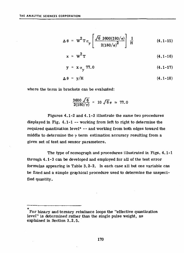
THE ANALYTIC SCIENCES CORPORATION
A 6 = W2 Ta 3600(180Ar)
2(180/Tr)2
x = W T (4.1-16)
(4.1-17)
(4.1-18)
y = xa 77.0
A6 = y/H
where the term in brackets can be evaluated:
3600/6" _2(l80/ir) ~
Figures 4.1-2 and 4.1-3 illustrate the same two proceduresdisplayed in Fig. 4.1-1 — working from left to right to determine therequired quantization level* -- and working from both edges toward themiddle to determine the y term estimation accuracy resulting from agiven set of test and sensor parameters.
The type of nomograph and procedures illustrated in Figs. 4. 1-1through 4.1-3 can be developed and employed for all of the test errorformulas appearing in Table 3.2-2. In each case all but one variable canbe fixed and a simple graphical procedure used to determine the unspeci-fied quantity.
For binary and ternary rebalance loops the "effective quantizationlevel" is determined rather than the single pulse weight, asexplained in Section 3.2.5.
170

THE ANALYTIC SCIENCES CORPORATION
4.2 DATA PROCESSING EQUIPMENT
Constant Motion and Sinusoidal Averaging — If testing isconfined to constant motion and averaging measurements made duringvibratory motion, the data processing requirements are relativelysimple. For each test run the net number of pulses, representing theintegrated torque, and the total test time must be recorded. Followinga sequence of test runs some linear algebraic equations must be solvedto yield estimates of the parameter groups and sensor parameters (seeEqs. (3.2-3) and (3.2-4)).
Sinusoidal Harmonic Testing — For sinusoidal harmonic testingthe data processing equipment required in the test laboratory is deter-mined mainly by the data processing phase la (see Fig. 3.1-3). Theother phases must await the completion of a sequence of single-axis testsand, therefore, will be performed off-line. (To the extent that some ofthis subsequent processing can lead to a quick determination if a test issuccessful, there could be a significant operational advantage in havinga limited amount of off-line capability readily accessible at the time thetests are being performed.)
From the point of view of laboratory equipment choices thereare basically two ways to perform data processing phase la:
• Record the sensor output data (and measurementsof test motion if desired) for later off-lineprocessing.
• Process the data on-line as it emerges from thetest, producing immediately a set of filteredestimates of the observable quantities (Fouriercoefficients).
171

THE ANALYTIC SCIENCES CORPORATION
In either case the leading candidates for a processing algorithm are theFourier analysis, the least squares estimation, and the Kalman filteringprocedures outlined in Section 3.4.
If the first method is used, the crucial equipment specificationsare those required of the recording equipment. They result chiefly fromthe high output data rate. For an analog rebalanced sensor feeding ananalog recorder, the recorder bandwidth must be higher than the firstfew harmonics of the maximum applied test motion frequency. It is notpossible at the present time to establish a quantitative requirementssince high frequency testing has not been investigated. For a pulserebalanced sensor feeding a digital recorder, it would be desirable to beable to record the complete sequence of pulses in order to make fulluse of the test data. In this case the required data recording rate issimply the maximum pulse rate used by the strapdown sensors under test.Consider the following numerical example: a maximum test time of 200seconds and a binary pulsed gyro with a pulse repetition rate of 5000pulses per second. The recorder must, therefore, have the capacity tostore a sequence of one million binary digits at the rate of one every 0.2milliseconds. Simultaneously it must record "timing marks" in aparallel channel, indicating the zero-reference points in the test motion
history.
If on-line processing is used the computer must be able toaccept data at the sensor output data rate and simultaneously, processequations like those of Section 3.4 at this same rate. This implies veryshort operation times for the computer used. The various sets ofequations for the sinusoidal coefficients [for example, Eqs. (3.4-4) and(3.4-5)] point up the need for careful time-synchronization between theoutput data and the applied motion. The "weighting factors," sin ncot and
172

THE ANALYTIC SCIENCES CORPORATION
cos ncot, must be cycled through 2im radians for each period of the test
motion, without drifting out of phase. Otherwise, the computation will
not be one of averaging m sets of properly computed Fourier coefficients.
Also, if either the least squares estimation or Kalman filtering equations
are used, the time-varying elements of the H matrix [see Eq. (3.4-29)]
must be kept in phase with the actual applied motion history.
Chapter Summary — Test motion machinery specifications may
be derived from an understanding of the manner in which test motion
errors propagate into parameter estimation errors and from the overall
test accuracy requirements,, The propagation of test motion errors for
constant rate testing, sinusoidal averaging and sinusoidal harmonic test-
ing are treated in detail in Section 3.2 Nomographs provide a convenient
way to make use of the error formulas summarized in Table 3.2-2. The
overall test accuracy requirements depend on the underlying reasons for
conducting a specific set of tests —whether they are research oriented or
mission oriented, etc. - as discussed in Section 1.1. The data process-
ing functions for constant rate testing and sinusoidal averaging are quite
simple. For sinusoidal harmonic testing the data processing equipment
specifications depend on whether off-line or on-line processing is used.
In the former case the recorder characteristics, which depend on data
rate and test time, are crucial. In the latter case the on-line computer
characteristics, which are dictated by the data rate and the detailed nature
of the estimation equations outlined in Section 3.4, are crucial.
173

THE ANALYTIC SCIENCES CORPORATION
5. CONCLUSION
5.1 SUMMARY OF FINDINGS
The starting point of this effort is a set of equations (derived in
Refs. 2 and 3) for motion-induced error torque in single-degree-of-freedom
(SDF) sensors. These error models have been manipulated in a way which
is valid for closed-loop, low-frequency testing, yielding error torque
expressions which are linear functions of a set of "basic parameter groups"
defined in Table 2.4-1. All of these basic parameter groups can theoretically
be identified and measured by means of a sequence of single-axis vibration
tests, including six angular vibration tests, and six linear vibration
tests. All but one of them are independent of test motion frequency
and magnitude. *
The following three types of single-axis angular-motion tests have
been studied in detail:
• Constant Rate Testing
• Sinusoidal Testing, Averaging
• Sinusoidal Testing, Harmonic Extraction
The bases for comparing the three types include the observable quantities
(measurable parameter groups), the amount of redundant data provided,
the number of test runs required, the degree of difficulty of data processing
*See the discussion in Section 2.4.1 of the effect of rotor speed control
loop dynamics on kjQ.
175

THE ANALYTIC SCIENCES CORPORATION
required and the accuracy with which various parameters can be estimated.
(A comparison summary is given in Table 3.2-3.) Constant rate testing isthe simplest to perform but does not produce the complete set of basicparameter groups. Sinusoidal averaging is simpler than sinusoidal har-monic testing but yields an even smaller subset of the complete list. Onlysinusoidal harmonic testing provides a measure of all the parameter groups.
The principal data processing function for both constant ratetesting and sinusoidal averaging is to compute average torque by generatinga net pulse count and dividing by the total time of a test run. For a sequenceof sinusoidal harmonic tests there are three data processing stages: thecomputation of Fourier coefficients defining the periodic applied torquefunction for each test run; the processing of the entire array of coefficientsfrom a complete sequence to produce the basic parameter groups; and thecomputation of individual sensor parameters. The first stage may beperformed by means of Fourier analysis, least squares estimation orKalman filtering (detailed equations for all three candidates are given inSection 3.4). The second stage is an "overspecified" algebraic probleminvolving redundant information. The extra data can be used as a cross-check on the operation of the test sequence or as a means to indicate theexistence of error torques not included in the model. The third stage is asimple algebraic problem.
Methods have been developed for analyzing the effects of varioustest error sources and of test duration on the achievable accuracy inestimating sensor parameters. Three classes of test error sources areconsidered: test motion errors, measurement errors and changes in thesensor parameters. Motion errors and measurement errors have bias,cyclic and high-frequency noise components, including the effects ofquantization. The resulting error formulas (summarized in Table 3.2-2)have been used in a set of illustrative numerical calculations based on an
176

THE ANALYTIC SCIENCES CORPORATION
assumed set of typical SDF gyro parameters. In these examples thenominal magnitudes of the coefficients of the third harmonic terms areextremely small, leading to the conclusion that the significant data fromeach vibration test will be contained in five Fourier coefficients (the biasterm, the coefficients of the sine and cosine terms at the fundamental testmotion frequency and the coefficients of the second harmonic sine andcosine terms). Constant rate testing or sinusoidal averaging appear to bemore accurate than sinusoidal harmonic testing in a number of cases.Sinusoidal harmonic testing provides good redundant measurements in thecases where the sensor input axis is nominally perpendicular to the testmotion axis. It also provides good measurements of parameters andparameter groups which cannot be determined by the other types of testing.In two situations sinusoidal harmonic testing appears to yield the mostaccurate estimates of parameters which can also be measured using one ofthe other techniques.
5.2 RECOMMENDATIONS
The apparent effectiveness of a combination of vibration testingand constant rate testing leads to a major recommendation of this study—that conventional single-axis devices should be given strong considerationwhen developing test procedures for strapdown inertial sensors. Someindications of quantitative test equipment specifications can be drawn from
the example test error calculations presented (these are summarized inSection 4.1).
177

THE ANALYTIC SCIENCES CORPORATION
While constant rate testing is by far the simplest to perform, it
is important that some cross-checking by sinusoidal averaging and probably
by harmonic testing as well, be performed. It may be desirable, for
example, to develop an operational calibration procedure using constant rate
testing to generate coefficients which will compensate for the effects of
system vibrations. The appropriateness of compensation so derived should
be verified by means of vibration testing, which more closely resembles
the dynamic environment to which strapdown sensors will be subjected.
If maximum benefit is to be obtained from harmonic testing,
either high speed recording equipment or high speed on-line, real-time
data processing equipment will be required in the test laboratory. These
would be needed to extract the harmonic content of the rebalance torque,
averaging data taken over many test motion cycles. A trade-off between
the sophistication of laboratory data processing equipment and the complexity
of motion-supplying devices is apparent. For example, a sequence of
single-axis vibration tests combined with data processing which extracts
harmonics, can substitute for multi-axis tests employing out-of-phase
vibrations.
An overall conclusion may be stated as follows: It appears
that useful information can be obtained from a sequence of practically
achievable single-axis vibration tests. However, the test error
analysis is only as good as the assumptions on which it is based, and it is
possible that some test error sources will be much larger than those
assumed in the example calculations, or that there are other important
error sources not included in the analysis. It is therefore recommended
that a set of feasibility tests be conducted as soon as possible. These tests
would apply low-frequency single-axis angular vibrations to an
178

THE ANALYTIC SCIENCES CORPORATION
analog-rebalanced SDF gyro and use available signal-processing equipmentto determine the harmonic content of the gyro output signal. The testresults should be used to answer the following questions:
• Do the magnitudes of the output harmonicsagree generally with predictions ?
• What are the most significant sources oftest error?
• What can be done, via test hardware modi-fications, to reduce these errors?
• After appropriate hardware modifications havebeen made, what is the "real" data processingproblem remaining? That is, what noise sourcesmust be filtered; or what cyclic or bias errorsshould be calibrated?
Besides verifying the practicality of the proposed type of testing, a series offeasibility tests would provide information which would be useful in guidingthe continuing analytic studies discussed below. These, in turn, wouldbecome more useful in producing realistic test laboratory equipmentspecifications and in developing appropriate data processing procedures.
Continuing studies related to low-frequency, single-axis test-ing of SDF sensors should be broadened in some respects and deepenedin others. The test error analyses should be developed into a parametricstudy, covering a range of sensor parameters and test motion quantities,with the goal of providing approximate indications of the test duration andequipment precision required to extract sensor parameters to specifiedaccuracies. Particular test situations with particular sensors should beanalyzed in detail, with the goal of making specific recommendations asto test procedures and data reduction techniques. A generalized simulation
179

THE ANALYTIC SCIENCES CORPORATION
capability would be useful in verifying analyses already performed and
in evaluating alternative data processing schemes.
A better understanding of motion-affected errors which are
mentioned in Section 1.1 but not included in the present error models, such
as those caused by scale factor changes and friction torques, should be
developed. These additional error terms will also be considered in devising
test procedures.
The potential advantages and difficulties of employing high-
frequency, single-axis vibration tests on inertial sensors should be
evaluated. An attempt should be made to re-formulate the data process-
ing problem discussed in Section 3.4 in a convenient way which does not
depend on the low-frequency assumption. A high-frequency test motion
error analysis should, if needed, also be developed. The goal of this
investigation would be to indicate if information concerning dynamic
instrument errors that is not revealed by well-designed low-frequency
tests can be extracted by high frequency tests, and if so, to provide
error analyses which can be interpreted in terms of test equipment
specifications.
The importance of stability of strapdown sensor parameters
suggests that the recommended tests be employed in a sequential fashion,
aimed at measuring stability. Strapdown sensors may only be calibrated
before installation in a vehicle (since they cannot be isolated from inci-
dental vehicle motions and reoriented relative to gravity and earth rate)
and a means must be available to predict, with known confidence limits,
the stability of the measured parameters. Stability will be a prime objec-
tive of the instrument designer, and tests which relate sensor design
features to coefficient stability will be of great value. Prior theoretical
work related to this subject should be reviewed and experiments for
evaluating mathematical models of parameter variation should be designed.180

THE ANALYTIC SCIENCES CORPORATION
APPENDIX A
DERIVATION OF TRIGONOMETRIC SERIES COEFFICIENTS:
VIBRATION TESTING OF SINGLE-DEGREE-OF-FREEDOM SENSORS
This appendix derives expressions for the Fourier coefficients
which are the observable quantities in single-axis angular and linear
vibration tests of single-degree-of-freedom (SDF) gyros and
accelerometers.
SDF Gyro: Angular Vibration — The general expression for
angular motion-induced torque in a SDF gyro is given as Eq. (2.4-5)
and is repeated here:
Mang = kl*L
Vs
7i 8~o 7~s
k14d)ocoi
where k.. through k-. are the basic parameter groups defined in Table 2.4-la.
181

THE ANALYTIC SCIENCES CORPORATION
A general single -axis angular vibration of amplitude W and
frequency to can be represented by:
to. = CjWsintot = WA sin cot (A-2a)
wo = c0
Wsin wt = W0
sin wt (A-2b)
to_ = c Wsin cot = W sin tot (A-2c)s s s
where c. , c and c are direction cosines relating the vibration axis toi o sthe gyro principal axes and W. is defined as c.W, etc.
The derivation consists of substituting Eqs. (A-2a), (A-2b) and(A-2c) into Eq. (A-l), term by term, and applying well known trigono-
metric identities, as shown by the following examples:
. cos tot (A-3a)
wio>0 = kgW.Wosin2 cot = kgW. WQ(1 - cos 2 tot) (A-3b)
0 O *3 1 9k12to.to = k12W.W sin tot = ^kjoW.W: (3sin tot - sin3 cot) (A-3c)
k14ioW8 = |k14Wo^wr°8a>
= | k14WoW?aj 1 cos tot (1 - cos2cot)
= rk14WoW2tol[cos cot - cos3wt 1
= |k14WoWia}liCOSa3t -^Cos3a5t " 3 cos cot) 1
= k W W 2 c o (cos tot - cos 3 cut) (A- 3d)
182
THE ANALYTIC SCIENCES CORPORATION
After treating all terms in Eq. (A-l) in the above fashion and groupingsimilar terms, we obtain:
M = B + St sin cot + C. cosang 1 1
+ S0sin2cot + C0 cos 2cot& ft
+ S0sin3a)t +0
(A-4)
where the seven trigonometric coefficients (Fourier coefficients) are:
B =
, = k.W. + k_W + kcW + |k10 (w3 - W.W2)1 4i 5o 6 s 4 12 \ i is /
(A-5a)
(A-5b)
Cl = k2Wo + k3Ws + ?k!4Wo(A'5C)
(A-5d)
*9wiwo + k W W + k W W! 0 i s l l o s ](A-5e)
(A-5f)
(A-5g)
183
THE ANALYTIC SCIENCES CORPORATION
SDF Accelerometer: Angular Motion —The general expression
for angular motion-induced torque in a SDF accelerometer is given inEq. (2.4-13) and is repeated here:
(A-6)
where k.. through kR are the basic parameter groups defined in Table 2.4-lb.
Equations just like Eqs. (A-2a), (A2-b) and (A-2c), except thatoj , c and W are used instead of co0, c and W , are substituted intop p p s s sEq. (A-6). After applying the same trigonometric identities, illustratedin Eqs. (A-3a) through (A-3d), and grouping similar terms, we obtain:
M = B + C, cos ostang 1
+ C0 cos2totCl
+ C<jCos3wt (A-7)o
where the four Fourier coefficients are:
184

THE ANALYTIC SCIENCES CORPORATION
B = £ I k, (W" - W" ) + kcW.W + kcW.W + k-W W 12 | _ 4 \ i p / 5 i o 6 i p 7 o p J
Cl = co | kjW. + k«W + k«W + ik«W. (W2 -2 o 3 p **8Wo ( W f
C0 = - ^ I k. fw2.- W2} + k_W.W + k.W.W + k^W W 1 (A2 2 | _ 4 \ i p / 5 i o 6 i p 7 o p J v
1 / 2 2\CQ = - TkoOsW WT - W (A-8d)3 4 8 o V i p/
SDF Gyro: Linear Vibration — The general expression forlinear motion-induced torque in a SDF gyro is given in Eq. (2.4-15)and is repeated here:
M = k.f. +k0f +k0flin 1 i 2 o 3 s
+ k.f2 + k,f2
4 i 5s
+ Wo + Vi's + VO'B <A-9)
where k. through kft are the basic parameter groups defined in Table 2.4-lc.
A general single-axis linear vibration of amplitude A and frequency
a? can be represented by:
f. = c. A sin cot = A. sin cot (A-lOa)
f = c A sin cot = A sin cot (A-lOb)
f = c Asincot = A sincot (A-lOc)s s s
185

THE ANALYTIC SCIENCES CORPORATION
Substituting Eqs. (A-lOa), (A-lOb) and (A-lOc) into Eq. (A-9) and regrouping,
we get:
_. = B + S1 sino)t + C0cos2o?t (A-ll)iin A &
where the Fourier coefficients are:
5As2 + k6A. Ao + k^. Ag + kgA^] (A- 12a)
S, = k,A. -f k-A,. + k,A (A-12b)1 11 fi O «3 S
= 1 [k4A2
C2 = - \ ? + k5As + k6AiAo + VlA. + k8AoAs] (A' 12c>
SDF Accelerometer: Linear Vibration - The general expressionfor linear motion-induced torque in a SDF accelerometer is given in
Eq. (204-16), which is identical in form to that of Eqs. (2.4-15) and (A-9),
except that f is used in place of f. The basic parameter groups k.p s ithrough kg are defined in Table 2.4-ld. Equations just like Eqs. (A-lOa),
(A-lOb) and (A-lOc) can be substituted into Eq. (A-9) to yield Eq. (A-ll),
exactly. The three Fourier coefficients, B, S1 and C2, are defined
exactly as in Eqs. (A-12a), (A-12b) and (A-12c), except that A appears
in place of A . Therefore:s
B = \ k4A2 + kgA2. + k6A. Ao + k^. Ap + kjA^J (A- 13a)
Sl = klAi + k2Ao + k3Ap (A-13b)
C2 • - I [k4Af + k5Ap + ViAo + k AAp + k8AoAp] 'A
186

THE ANALYTIC SCIENCES CORPORATION
APPENDIX B
TEST MOTION BIAS ERROR ANALYSIS:
ANGULAR VIBRATION TESTING OF
SINGLE-DEGREE-OF-FREEDOM GYRO
This appendix describes the effects of bias test motion errorson the Fourier coefficients defining the applied torque function duringsingle-axis angular vibration tests. The test motion errors consideredare errors in the knowledge of amplitude and frequency of the appliedmotions and misalignments of the test motion axes.
Derivation Overview - The derivation begins with Eqs.(A-5a)through (A-5g) of Appendix A. These equations relate the 7 Fouriercoefficients to the gyro parameters and the test motion quantities forthe general in-phase case:
(B, sr cv s2, c2, ss, c3) = f (kr..k14, w., wo, ws, w) (B-D
where represents the seven given functions.
The derivation proceeds in three major steps as follows.
First, partial derivatives are taken with respect to the motion quantitiesto yield 7 perturbation equations which can be expressed in one vectormatrix equation:
187

THE ANALYTIC SCIENCES CORPORATION
6W.i
6W= M
6W
6B
«!f>cl
6C2
6C3
where the elements of M1 are expressions involving the k's, W., W , Wi i o s
(B-2)
and co.
Second, Eq. (B-2) is transformed into the form:
6W
(B-3)
s
6 to
which relates the Fourier coefficient errors to test motion magnitude andangle errors, rather than component errors.
Finally, Eq. (B-3) is specialized for the six test axis orientationsof interest and reduced to the form:
188

THE ANALYTIC SCIENCES CORPORATION
6W
(B-4)
The test axis misalignment angles, e., and €«, have different meanings ineach case. If the test axis is one of the principle axes (say i), then c.. ande« are simply the misalignments about the other two (o and s). If the testaxis lies midway between two principle axes (say i and o), then e1 is themisalignment about the third (s) and €„ is the misalignment about the axisperpendicular to both the test axis and the c« axis.
These three steps are followed in detail below, concluding withsix equations (B-8a) through (B-8f) giving the expressions for the elementsof the matrix M« for each of the six test motion axes of interest.
Derivation Details — Equations (B-5a) through (B-5g) give theseven perturbation equations obtained by taking partial derivatives ofthe seven equations, (A-5a) through (A-5g). Equations (B-6a) through(B-6e) develop the relationship of component errors (SWj, 6WO, 6WS)to magnitude and angle errors (6W, q, eo, cs). The three relationsof Eq. (B-6e) were substituted into the perturbation equations to obtainnew perturbation equations, as shown in Eqs. (B-7a) through (B-7g).Table B-l summarizes facts needed to specialize the perturbationequations to the six tests of interest. Finally, Eqs. (B-8a) through(B-8g) present the seven perturbation equations in vector-matrix formfor the six cases.
189

THE ANALYTIC SCIENCES CORPORATION
6B =
[k8Wo-ik9Wl+ikllW.]SWo
[-k7Ws+2k10Wi+5kllWo]6Ws
[0] 6w (B-5a)
,2 3 6W.
+ Viki2wiWs] 6W
(B-5b)
[klWi + k2Wo + k3Ws + ?k!4Wo (B-5c)
6S0 • = k13Ws 6Wo[0]6W.+[|k13Ws]
+ [lk13Wo]6Ws+[lk13WoWs]6»
190
(B-5d)

THE ANALYTIC SCIENCES CORPORATION
[0] 6to (B-5e)
|"-£k1A w 2 -w 2 l|_ 4 14 i s J
[fk14WoWs]6Ws
ewo
6W
191
W = W.l. +W1 +W1 (B-6a)
W = W !„ = W (c.I. + c 1 + c I ^ (B-6b)W V i i o o s s /\ /
6W = W 61W + 6W lw = 6W.I + 6Wlo + 6Wgls

THE ANALYTIC SCIENCES CORPORATION
K -2618
Figure B-l Test Axis Misalignment Angles
The direction cosine errors are, from Fig. B-l:
6ci = Vo - Vs
6c = c. e - c e.o i s s i
6cs = Vi - Vo (B-6d)
Therefore:
6W. = c.6W - Wcoes
6W = c 6W +Wc.e - We e.O O IS 81
6W = c 6W + We e. - We. eS S O 1 1 O
(B-6e)
192

THE ANALYTIC SCIENCES CORPORATION
6B = W (k7c. - ik9CQ + ik10cg) (c. 6W
+ W ("I Vi + Vo + f kll°s) (co6W - WVi + Wi
+ W(lk10ci + lkllco - k7cs) (cs6W + WVi - WVo)
+ (0) 6W
= W k7c + kgc - k7c - k9c.co + k10c.cs + kncocs 6W
+ [^l^o + Ik10cs - 2kllcico + 2Vics - (k7 - k8)cocs] fi
+ W2[fk10cl + Ik10cs - 5kllVo + 2Vics - lVoc.] fo
+ w2 [-K6,2 + I V2 ' (k7 + ke) cico + 5kllcics - 5k10cocs] fs(B-7a)
' [k4 +(?k!2Ci - IB0')^] (CiW + Wcsfo - WVs)
+ l"k,l (c 6W - We <r. + Wc.c }|_ 5j \ o si is/
+ Fkc - Ik10c.c W2 1 (c 6W + We c. - Wc.e }[6 2 12 i s J \ s 01 107
+ [0] 6o>
" [k4Ci + k5Co + Vs +(!k!2Cf - ?k!2ci cs W 6W
[(k4cs - k6cl) W + (I k!2c12cs - I k!2cs)
k4co + k5ci) W + (-!k12cfco + f k12V
6W (B-7b)
193

THE ANALYTIC SCIENCES CORPORATION
6C. - to c - We .s o o s)
co6W - W»[*a + (?k14cf - ?k!4
">[k3 ' 2k14Cocsw
[(Vl + k2co + k3cs)W +(?k14coc2 - I^
. + Wc.e \i i sj
Cs8w + wVi - WVo
— * • I lr r> 4- lr f* - 1 - T r PtO ft-* Vx. ~ t\.~\^ T l^n^
1 1 1 Z o 3s k!4cf co - !k!4 Vs
-ik14ej2cs + J^cJ - i^cjc,) W3]
,c - koC.W -ik-.c-c c W3]e1 s 3 i/ 4 14 i o s Jo
K \ / 1 9 1 ^ 1 9 \ ^ 1
-klco + k2Ci) W + (-Ik14cico + 5k14Ci - ?k!4cics) W J
) w +(?k14^co - Ik14coci + Vo + k3cs
6S2 = (0) 6W.
' "[k!3cocsW]
k!3<=2^-
W2"k r rK13cics 2
k c2K13Cs
*s +
w2]2
k!3
Cj + CO
cc Wo s 2
2"
k cc W2XV^ A \^. ^ **13 i o 2
6 co (B-7d)
194

THE ANALYTIC SCIENCES CORPORATION
6C, = [(Vi + k9Co - k!0Cs) W] [Ci5W + WVo - WVs]
+ [('Vo + k9ci - kllCo)W] [Co6W - WVi + WVs]
+ K-k_c - k,nc. - k--c W] I c 6W + We e. - Wc.cL\ 7 s 10 i 11 oj J [ s 01 i oj
[0]
= W [k7Cf - Vo * Vs + k9cico - k!0cics - kllcocs] 6W
+ w2
+ W2
w
-KlCo + kllCs - KoCiCo - ^k9CiCs + (k8 * k?) Vs] eiJ
-4-^k n^ —Ic r' + —k rr + 9k r r + — k r rL 2K10Ci " 2K10Cs 2K11 Ci o ^K7 Cis 2K9 o sj
1, 2 1. 2 /. ^,"2kQCi ' 2kQCn " Vk7 +l
£1 a 1 & o \J \ ICico - Ikllcics +
[0]6o!
5S3 = - [•,6W
-3k c3
+ 3]4K12Ci 4 J LCsl6W
+ W ^1
[•*+ w3 [4k12c3 -
(B-7e)
[0] (B-7f)
195

THE ANALYTIC SCIENCES CORPORATION
e - We €so o s
+ to V.k C
4K14Cic 6W - We e. + Wc.eo si is.
+ (B-7g)
196

THE ANALYTIC SCIENCES CORPORATION
TABLE B-l
SPECIALIZATION TO SIX CASES OF INTEREST
^€i ' €o' *s' ~ '€1' €2'
'2
c.
w. = w
wo = w
w. =
w. = w =1 S
w = w =o s
1
0
0
1
0
10
1
V*"
0
0
1
0
1
clf
197

THE ANALYTIC SCIENCES CORPORATION
Angular Vibration about the Output Axis
(W0 = W, c0 = 1)
6B
8Si6C,
6S,
«C2
«s3
A
=
kgW
k5
«*2
0
-k8w
0
0
Ik W2
2K11
k6w
o*3w
w^
-Ik W2
2 11
0
0
iv*-k4w
-^w
0
-h*2
0
0
0
0
V
0
0
0
0
6W
603
(B-8a)
Angular Vibration about the Spin Axis
(Wg = W, cs = 1)
6B
5Sl
«Cl
«s2
6C2
6S3
_«c3_
=
-k?W
k6
Wk3
0
+k?W
0
0
-Ikllw2
kgw
-(k2W + lk!4w3)
-cok ^
+lknw2
0
-4k!4w3
\\yk* W - -k WK4W 4K12W
wklw
0
-KcXIk W3
4k12W
0
0
0
k3w
0
0
0
0
6W
€i
eo
6u)
Dominant Term.
*B-8b)
198

THE ANALYTIC SCIENCES CORPORATION
Angular Vibration about the Input Axis
(Wi = W, Ci = 1)
6B
6S1
6C
6S2
6C2
6S3
!c*.
-
^^KX
tok,1
0
-k?W
3 J2-4k12^
0
-ik W2
2K10W
-k6w
-a* W3
0
^K/
0
0
-K-2
kcW0
w(k*w + lk W3)2 4 14
0
-K"2
0
0
0
0
k W1
0
0
0
6W
eo
€s
6.
(Angular Vibration about Output and Spin Axes
(W0 = Ws = W/yi, C0 = cs = 1//2)
6B
6S
6C
ac
W
5 6
co (k!+k3)-7=-|i[ 2 3 A^ 8 -
wwk!3T
W2
(k +k )-5 6
w2
W3
2 1 0
V* W - _k Wk4W 8k12W
(B-8c)
- - . , -A/2 8 14A/2
W3
8W
(B-8d)
Dominant Term.
199

THE ANALYTIC SCIENCES CORPORATION
Angular Vibration about Input and Output Axes
= c0=l//2)
SB
fiS,
6S.
ec.
6C,
W
3k W3
1, W3
10.
> /£
»w
W2
2 l l
4*14^
Angular Vibration about Input and Spin Axes= Ws = WA/2, ci = cs = 1/-/2)
Dominant Term.
6W
6(0
(B-8e)
6B
6Sj
eCj
2
6C2
6S3
3
— k W2K10W
(k*+kg)-^-|k12^
1uKkj+kj)— -=.
0
-IV
0
0
j_ if \X/> JVM "
4 6V2
/, , > Ww(kl'k3)~7=1 3Vz
0
-^
0
0
X,-v^0
0
2Wk13V2
-2(kirk9}^|
1 W3"8K12W
4k14w3
0
0
0
0
0
0
6W
€o
€P
((B-8f)
200

THE A N A L Y T I C SCIENCES CORPORATION
APPENDIX C
KALMAN FILTERING FORMULATION
For the single-axis vibration tests described in Chapter 3, thefirst data processing stage (see phase la in Fig. 3.1-3) is one which ac-cepts as input the scalar, periodically time-varying gyro output and pro-duces as output the set of Fourier coefficients defining the applied torquefunction. This appendix formulates this data processing function as aproblem in linear estimation for which the Kalman filter is an optimalsolution. The filter equations, which could be used for processing actualtest data, are presented. A hypothetical situation in which there is noprocess noise is used to demonstrate the trade-off between test accuracyand test duration, and to show a connection between this type of processingand classical Fourier analysis. Finally, the full problem, with bothmeasurement noise and process noise is treated and some approximateequations, which are useful in predicting the achievable test accuracy and
required test duration, are developed.
201

THE ANALYTIC SCIENCES CORPORATION
C.I FILTER EQUATIONS
In this section the estimation problem is formulated in mathe-matical terms and the optimal solution is stated in the form of a set ofdifferential equations, the Kalman filter equations, which can be mechanizedto process data. No proof is given here for the optimality of this solutionsince it is well documented. (See, for example, Ref. 8.)
The problem formulation requires three things: a linear meas-urement equation, a linear state differential equation and a description ofthe statistics of the random variables defined in these two equations. Ascalar time-varying signal (torquer current) is measured which, except forerrors in the measurement process, is proportional to the output of thetorque generator. Therefore, the measurement equation is (See App. A.):
z = M + erroro
= B + S.. sin tot H-C
+ S2 sin2 cot + C, cos2 tot
+ S, sin3 tot + Cg cos 3 tot
+ error (C.l-1)
which can be rewritten:
202

THE ANALYTIC SCIENCES CORPORATION
z =
x4h4(t) + x5h5(t)
+ v(t)
. = Hx + v (C.l-2)
The components of the state vector x are the 7 Fourier coefficients. Theelements of the measurement matrix H (in this case a row vector) are theset of time -varying functions (1, sin cot, cos cot, sin 2 cot, . . . ). We assumethe measurement noise v to be Gaussian white noise with zero mean andcovariance r6 (t - T), where 6 is the Dirac delta function:
v(t) = 0j v(t)v(T) = r6( t - r ) (C. 1-3)
Before discussing the state differential equation and processnoise we distinguish between the following two test situations. In case athe only data produced by the test is that representing the time historyof the gyro torquer output, and it is natural to define measurement noiseas above. No measurements of test table angle are generated, and it isalso natural to regard fluctuations in the applied test motions as one sourceof process noise. In case b both gyro rebalance torque and test table anglemeasurements are generated. In formulating the estimation problembelow, however, we continue to treat gyro torque measurement errors asthe only source of measurement noise and we regard table angle encodererrors as a source of process noise. This point of view avoids morecomplex calculations which would arise if we expanded the measurementequation to include table angle measurements.
203

THE ANALYTIC SCIENCES CORPORATION
Case a
The state equation is the seven-dimensional vector differentialequation expressing the rates of change of the seven Fourier coefficients.The state equation is:
where the process noise vector u is also assumed to be Gaussian whitenoise with:
u(t) = 0; u(t)u(r) = Q 6 ( t - r ) (C.l-5)
There are two ways in which process noise can occur. Consider the fol-lowing specific example of a single-axis angular vibration test. The testmotion axis is midway between the gyro output and spin axes; the appliedangular rate is given by:
W
Based on the expressions given in Table 3.1-1 we can write for themeasurement equation:
204

THE ANALYTIC SCIENCES CORPORATION
Z =
W
•Tz (Vke) sin cot
-Kj cos tot
13 sin 2 cot
cos 2 cot
+ [0]sin3 cot
l48
v(t)
cos 3 co t
(C.l-7)
The terms in the brackets are the seven state variables in this example.They can vary either because the basic parameter groups (the k.'s) varyduring the test or because the test motion amplitude and frequency (Wandco)vary during the test. If test motion variations are the major cause ofprocess noise, the various components of the noise vector will be highlycorrelated since W appears in all six non-zero state variable definitionsand co appears in three of them. That is, the off-diagonal elements of theQ matrix will be non-zero and significant. If, on the other hand, gyroparameter changes are the major cause of process noise, we would expect
205

THE ANALYTIC SCIENCES CORPORATION
very little correlation between process noise components; the only exceptionbeing a strong correlation between the first and fifth components becauseboth depend on parameter groups k-, kg and k.....
Since both the state equation and the measurement equation arelinear (with time-varying coefficients in the latter), and since the processand measurement noises are assumed to be Gaussian, the Kalman filter isthe optimal way (minimum variance estimation error) to process the meas-urement data. The applicable form of these equations may be written:
x = K [z - Hx ]
1 T= -PHr
= Q--PHTHP
(C.l-8)
(C.l-9)
. (C.l-10)
where x is the optimal estimate of the state vector x, K Is the Kalmanfilter gain matrix (7x1) and P is the covariance matrix of the estimationerror:
= ( x - x ) ( x - x ) J (C.l-11)
The integration of Eq. (C. 1-10) yields curves like that illustrated in Fig. 3.3-3.
206

THE ANALYTIC SCIENCES CORPORATION
Case b
We now consider the situation in which table angle measurementsare generated. In the following formulation Eq. (C. 1-10) still applies, butwith a modified interpretation for the process noise matrix Q. Consider thethird state variable in the above example:
Differentiating:
o .
We will consider the test motion changes, W and to , as control functionswhich change the values of the state variables (Fourier coefficients). Theindicated values of these control functions, which are derived from testtable measurements, enter into the filter equations as a control vector.Following the development in Ref. 7, Section 2.2, "State EstimationWithout Measurements, " we can write for the state equation:
x = u= Fx + Guk+ Lp_
[See Eq. (2. 2-6) in Ref. 7.]
where, in this case:
207

THE ANALYTIC SCIENCES CORPORATION
F = 0
u. represents random "system disturbances," or changes~~ in the values of the parameter groups (fcp ... fc^)-
p represents the "control function, " or test motion changes(W, co).
G is a 7 x 14 matrix whose elements are terms like wW/V~2"
L is a 7 x 2 matrix whose elements are terms like
Following Eq. (2.2-8) in Ref. 7, we can write:
0 0P = / P + P /T + GQ,GT + LSLT (C.I
/ ' K
where:
uk(t)uk(T)T = Qk6(t-T) (C.l-16)
and:
[P(t) - Pind(t)] [p(t) - Pind(r)]T = S 6( t -T ) (C. 1-17)
We define the effective, overall process noise matrix as:
GT + LSLT (C.l-18)
where GQ,G represents the contribution of random changes in the gyro
parameters and LSL represents the contribution of "errors in the applied
control, " i.e., errors in the indicated test motion. We have adopted
the following point of view. The indicated history of test motion, de-rived from the table angle measurements, is regarded as the "desired"
control function. The difference between the actual and indicated motion
208

THE ANALYTIC SCIENCES CORPORATION
changes can then be regarded as the error in the applied control. This
error is effectively a process noise in this formulation.
Together with the modified interpretation of the process noise
matrix Q, Eq. (C. 1-10) must be modified to account for the effect of theindicated, or "desired," control:
x = K[z - Hx] + Lp (Co 1-19)
C.2 TEST TIME VS ACCURACY
For the hypothetical situation in which there is no process noise
(Q = 0) Eq. (C. 1-10) reduces to:
P = - l p H T H P (C.2-1)r
Since the derivative of the inverse matrix can be written:
• -1 -1 • -1P = -P PP x (C.2-2)
we can write:
P"1 =-P"1PHTHPP"1
r
= ^H A H (c.2-3)
Based on the definition of H we have:
209

THE ANALYTIC SCIENCES CORPORATION
HTH =
sin2t,-t
sinu-tcosu-t sine,-tsia 2t j<l sinu-tcos 2u.'t
sin3u-t
' tsin2£i ' t cosa't cos2a-t cos a- 1 sin 3u.-t
symmetric
sin2a:tcos2a;t
2cos 2a- t
2sin 3tt-t
cos3a-t -
inu-t cos 3a-t
cos 3u:t
t cos 3o*t
ocos 3 a- t
(C.2-4)
Notice that the off-diagonal elements are products of two time functions which
are orthogonal over one test motion period, T = 27r/cc (the integral of theTproduct is zero). The integral of the matrix H H over exactly one period
is, therefore, the diagonal matrix:
It = (n + l)T
HTHdt =
t = nT
I2 1
2 12 1
2
O
2 12
(C.2-5)
Therefore, the change in the inverse covariance matrix over one cycle cfthe test motion is:
210

THE ANALYTIC SCIENCES CORPORATION
i2 1 o
o12 1
2 1.2 1
2
(C.2-6)
and
P"1(nT) =
12 1
2 I2 1
2
O
2 1 .2
(C.2-7)
where n is the number of cycles since the start of the test. After sufficienttime has elapsed the second term of Eq. (C. 2-7) dominates the first term,
P" (0), allowing us to write the approximate expression:
t -»large
Oj.2 j.
2 1.2 1
2 12 1
2O
(C.2-8)
The covariance matrix then becomes (taking the inverse of the inverse):
211

THE ANALYTIC SCIENCES CORPORATION
P(t) « ft -» large
"l2
2
O
o"2
22
2
(C.2-9)
Thus, for the no-process-noise case, the simultaneous estimation of theseven state variables, x1 through x^, separates into seven scalar problemsfor which the rms estimation errors are:
11rt (C.2-10)
and
P..112rt (1 = 2 ,3, . . .7) (C.2-11)
Equation (C. 2-11) illustrates the trade-off between test time and test accuracyas a function of the measurement noise.
212

THE ANALYTIC SCIENCES CORPORATION
C. 3 CONNECTION WITH FOURIER ANALYSIS
The analysis of the preceding section can be extended slightly to
demonstrate an interesting connection between optimal filtering and Fourier
analysis techniques.
The combination of Eqs. (C. 1-9) and (C.2-9) yields the following ap-
proximate expression for the filter gain matrix:
Kt •* large
1 T= -PHr1f-t
2 sin co t
2 cos cot2 sin2 cot
2 cos 2 cot
2 sin 3 co t
2 cos 3 cot
Substituting Eq. (C.3-1) into Eq. (C. 1-8) yields:
12 sin cot
2 cos cot
2 sin 2 cot
•e0
Z -
1
2 sin cot
2 cos cot
2 sin 3 co t
••0
(C.3-1)
-i [1 sin cot cos cot ...]
(C.3-2)
213

THE ANALYTIC SCIENCES CORPORATION
Integrating Eq. (C.3-2) over one cycle, and treating -^ and x as constant over
this time yields:
nT
1
2 sin cot
2 cos totzdt - IxT
In Fourier analysis the coefficients are determined by:
T
zdt
oT
. dto
T2 /•
Cn = T I zcos(n"t) dt•o
See, for example Ref.9. Also t^ nT. Therefore:
= |
n = T f zsin(nw
/\ JL.Ax ^ = —-n+1 n
Fourier estimate of xbased on (n+ l)st cycleof data.
- x-n
and:
(C.3-3)
(C.3-4)
(C.3-5)
(C.3-6)
(C.3-7)
x,i = x + Ax -—n +1 —n —n +1(C.3-8)
214

THE ANALYTIC SCIENCES CORPORATION
Thus, after sufficient time has elapsed, the optimal filtering equation be-
comes approximately Eq. (C, 3-8), in which the state vector estimate xbased on n cycles of data is adjusted by a weighted (1/n) difference between
the Fourier estimate based on the n + 1s* cycle of data and the previous
estimate o
C.4 STEADY STATE SOLUTIONS WITH PROCESS NOISE
We now consider the effects of process noise, represented by thematrix Q in Eq. (C. 1-10). The elements of the Q matrix along with the meas-urement noise r determine the final value of the elements of the P matrixas well as the settling time, t . Note that the rms estimation error of thesi^1 state variable is the square root of the i*h diagonal element of the co-variance matrix:
(C.4-1)
Equation (C.l-10) represents n (n + l)/2 simultaneous first-orderordinary differential equations which are nonlinear (since P appears twice
in one term) and which contain time varying coefficients (the elements of•
H). The elements of P cannot reach constant values (with P = 0) since theelements of H change continuously. They can, however, reach a steady-
state solution in the form of an oscillation about average values.
The most evident way of investigating these steady-state solutions
is to numerically integrate Eq. (C. 1-10) via computer, starting from variousinitial values. Some examples of such integrations for one- and two-
dimensional versions of the problem are illustrated in Figs. C-l and C-2 and
discussed below. We can achieve an analytic indication of the final average
values by making some simplifying assumptions as follows.
215

THE ANAIYTIC SCIENCES CORPORATION
(D
(r =&(D<Iq =
f r =
(q =
100
10
10
100
44.7 = V2rq
Figure C-l Numerical Integration Results
Consider, first a one-dimensional version of Eq. (C. 1-10) wherewe are trying to estimate a single variable, the magnitude of a sinusoidaloscillation:
p (t) = q - V(t)p2(t) (C.4-2)
where
h(t) = sin (C.4-3)
The scalar p is the variance of the estimation error and the scalar q charac-2
terizes the process noise. We set h equal to its average value (1/2) and letp = 0 to obtain the steady-state equation:
0 = * - 27Pss (C.4-4.)
216

THE ANALYTIC SCIENCES CORPORATION
r = 10
- 100
"22 =
P22ssfrom E(1-(C:. 4-ieJ
1.4140.617
C12
00.9
) Exactf Solutions
t (sec)
Figure C-2 Improvement in Small Term Estimate Due to Correlation
Therefore:
(C.4-5)
The validity of this solution is demonstrated in Fig. C-l where integrationsof the exact equation, Eq. (C.4-2), are plotted for four combinations of r, q
and p (0). Note that while the steady-state value is apparently the same in
all cases, it is approached much faster with the smaller measurement noise,
r. Also note that the true steady-state solution is more oscillatory with
the higher ratio of q/r. (Oscillations are also present in cases (T) and (2)
but are too small to be seen in the figure.)
217

THE ANALYTIC SCIENCES CORPORATION
Consider next the two-dimensional problem in which a largevariable (Fourier coefficient), x.,, is multiplying sin tot and a small variable,x« is multiplying sin 2 cot. We refer to x. as the "dominant term" and x2 asthe "nondominant term." In the following development the process noiseq^j associated with x.. is assumed to be much larger than the process noiseq22 associated with x«. [This would be true whenever test motion amplitudevariations are the major cause of process noise; see Eq. (C. 1-7).] Theoff-diagonal element q12 of the process noise matrix can take values betweenzero (no correlation between process noise components) and(perfect correlation). Equation (C. 1-10) now becomes:
12
'12 P22 22
1r
pllP12
sin tot sinco t sin 2 co t
. 2sintotsin2tot sin 2tot
'11
(C.4-6)
We let the time varying elements of H H take their average values:
2 2 1sin tot = sin 2cot =• -s (C.4-7)
and
sinaitsin2cot = 0 (C.4-8)
218

THE ANALYTIC SCIENCES CORPORATION
We also assume:
11 22ss ss(0.4-9)
which is borne out by the results below if q11 » q09. Therefore:1 1 fli
pn +p22 « pn (C.4-10)
with the assumptions of Eqs. (0.4-7), (0.4-8) and (C.4-10), Eq. (0.4-6)becomes equivalent to the three scalar equations:
1 2
• = _L 2 2P22 q22 " 2r P12 P22
Setting the three left-hand-sides equal to zero yields the steady-state
solution:
ss(0.4-12)
'12ss
2r (0.4-13)
22ss2r q22 " q11
(0.4-14)
219

THE ANALYTIC SCIENCES CORPORATION
Equation (C.4-12), giving the steady-state variance of the dominant term, is
the same as Eq. (C.4-5) for the one-dimensional case. Equation (C.4-16)
giving the steady-state variance of the small term, reduces to Eq. (C.4-5)
when the cross-correlation term, q12, is zero. Thus, we can write:
(C.4-15)
where A. accounts for an improvement due to correlation between the
various components of process noise. A conservative formula for the
final value of the estimation error for the i^1 state variable is, therefore:
(C.4-16)
The settling time (defined in Section 3.3 and illustrated in Fig. 3.3-3) associatedwith this level of accuracy may be found by setting Eq. (C.2-11) equal to
Eq. (C.4-16) and solving for t, yielding
(C.4-17)
Equations (C.4-16) and (C.4-17) are plotted parametrically in Fig. 3.2-5.
220

THE ANALYTIC SCIENCES CORPORATION
An alternate form of Eq. (C. 4-14) is:
02 = ss
where c.g is a measure of the correlation between the two components ofprocess noise:
— (C.4-19)
V °l
The corresponding expression for a useful test time is:
(C.4-20)
The validity of Eq. (C.4-18) is demonstrated in Fig. C-2 where integrations
of the exact Eq. (C.4-6) are plotted for two values of the correlation
measure (zero and 0.9).
In summary, through the use of simplifying assumptions we
have developed a set of formulas which provide useful indications of the
final steady-state estimation accuracies, Eqs. (C.4-16) and (C.4-18), and
the corresponding settling times, Eqs. (C.4-2) and (C.4-6), for one- and
two-dimensional versions of the estimation problem. Comparison of
Eqs. (C.4-18) and (C.4-20) with Eqs. (C.4-16) and (C.4-17), respectively,
221

THE ANALYTIC SCIENCES CORPORATION
shows that a strong correlation between process noise components reducesthe final estimation error of the nondominant term but increases the timeneeded to reach the more accurate level. The validity of the above formulashas not been checked for the n-variable case where n > 2. It is felt, how-ever, that the formulas will remain valid since the two-dimensional casecontains the essential ingredients of the problem.
222

THE ANALYTIC SCIENCES CORPORATION
APPENDIX D
FOURIER ANALYSIS EQUATIONS FOR
PULSE REBALANCED TESTING
This appendix derives two sets of exact equations which producethe Fourier coefficients of the torque generator output produced during vi-bration testing of a pulse rebalanced sensor. The first set corresponds tothe binary or ternary pulse-torquing scheme; the second set correspondsto the time modulation scheme. The torque produced by the rebalanceloop opposes the total "applied" torque, which is the sum of the desiredgyroscopic or pendulous torque and all disturbance torques. Since theapplied test motion is periodic and the residual (non-motion-induced)torque is assumed to be constant over the time of the test, the total appliedtorque is assumed to be a periodic function of time.
D. 1 BINARY AND TERNARY PULSE-TORQUING
Figure D-l pictures typical waveforms of the applied torque,M , and the torque generator output, M. , as well as their integrals, for
a. igthe binary pulse rebalanced case. The two integral functions are forced,by the action of the closed loop, to have the same low-frequency harmoniccontent (both consist of the ramp, Bt, plus a periodic function). The twotorque functions, M and M. , must also have the same low-frequency
a. Lg
description, even though they appear quite different in form. The de-•
rivative of the torque generator output, M. , consists of a sequence of
223

THE ANALYTIC SCIENCES CORPORATION
- 1230
= M fg^ B-t-S,sin<i>t +C ]coso)t+...
M
(a) Torque Waveform
/Mdt
S, C,/ M tgdt =/ Mad t S Bt + j3-(1 -cos a)t) + -jj- sinwt
Time
(b) Integral of Torque
M, Mtg = CjCOSwt + S^sin
an n tot- w C S i n o>t.+ ,
(c) Derivative of Torque
Figure D-l Binary Pulse Rebalancing Waveforms
224

THE ANALYTIC SCIENCES CORPORATION
impulse functions, as shown at the bottom of the figure. It must also be a
periodic function since it is the derivative of a periodic function. Its trigo-nometric coefficients (§j, Cj, etc.) are related to the torque function co-
efficients as shown. That is,
C = tonS (D.l-2)n n
We can conveniently apply classical Fourier analysis to the
derivative function. Thus, looking at one test motion cycle, lasting time,
T = 2 IT/CO , we can write:
TS =i j r f M(t)sinnwtdt = M(t)sinnootdt (D. 1-3)
*o
~ 2 rT - , , rT-C =£ I M(t)cosncotdt = / M(t)sinnwtdtn L *o Jo
A single square pulse, starting at time t., lasting one pulse
width, h, and of magnitude M. has the form sketched below.
225

THE ANALYTIC SCIENCES CORPORATION
Mtg
M.
t t. +hi i
t. = hi
Mtg
M. 6(t- t . )
-M. 6 (t -1. - h)
The derivative function consists of equal magnitude positive and negative
impulse functions spaced h seconds apart. The contribution of these two
impulses to the integral of Eq. (D. 1-3) is:
AS = — sinntot. - sinnwfc +h)n. ir [ i x J
= — sinntoh. - sinno)h(i + l)TT 1
(D.l-5)
Note that M. can take on either of two levels for binary torquing and any
of three levels for ternary torquing, according to:
M. =
M for a positive pulse
0 for zero torque
-M for a negative pulse
226

THE ANALYTIC SCIENCES CORPORATION
Adding up contributions like that of Eq. (D. 1-5) over one full
cycle of k pulse eidths, where k = T/h, we obtain:
k- 1
8 =^n TTi =0
M. [sinncohi - sinntoh (i + 1)1 (D. 1-6)i [_ J
Now, using the identity:
sin (a + B) = sina cos 0 + cos a sin£ (D. 1-7)
we obtain:
k - 1
S = — f ^ M. (1 - cos n ton) sinn oo hi - sinncoh cosncohi
i = 0(D.l-8)
Averaging over m full cycles, or km pulse widths, we obtain:
mk-1
S = s M. (1 - cosntoh) sinnojhi - sinnwh cosncohin m IT £^ i |_ Ji = 0
(D.l-9)
227
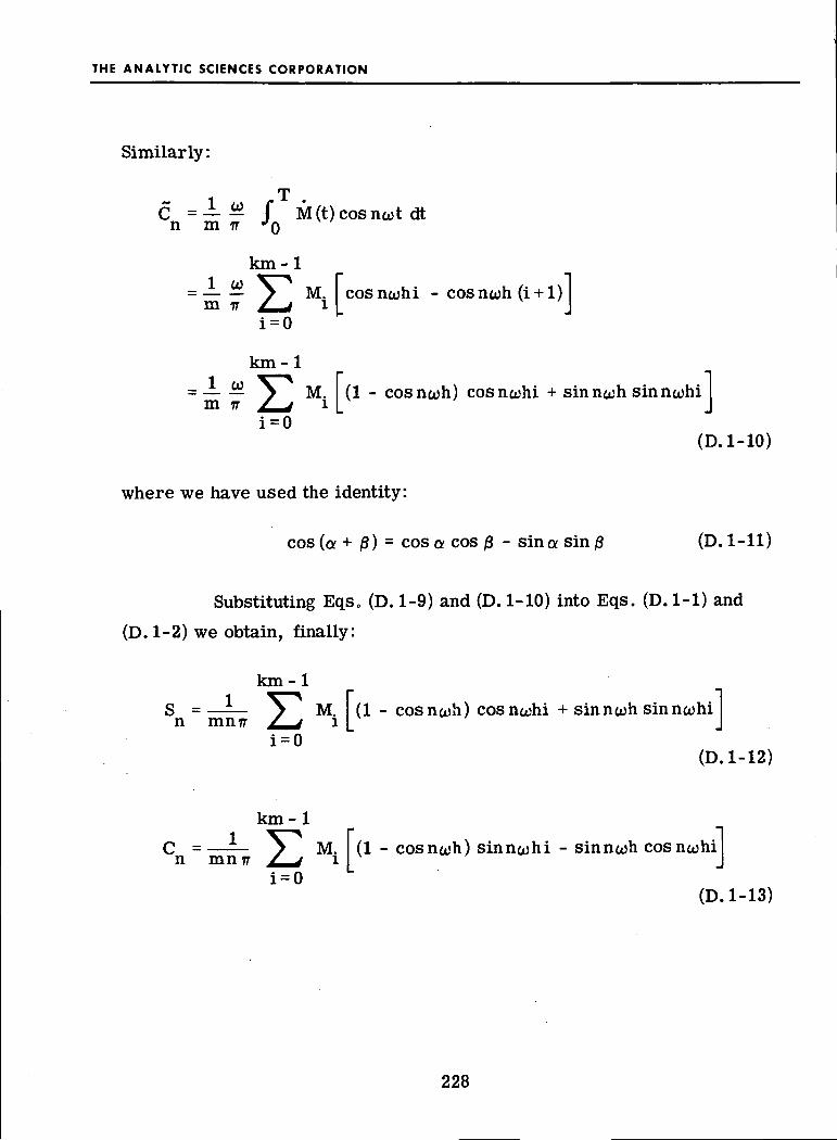
THE ANALYTIC SCIENCES CORPORATION
Similarly:
C =— - f M(t)cosncot dtn m IT JQ
km-1
= — — 7m TT f *
i = 0
M. cos ncohi - cos nwh (i + 1)i |_ J
km-1
= — — 7 M. (1 - cosncch) cosnwhi + sinncoh sinncohim 77 / j i |_ J
(D.l-10)
where we have used the identity:
cos (a + j3) = cos a cos 0 - sin a sin 0 (D. 1-11)
Substituting Eqs0 (D. 1-9) and (D. 1-10) into Eqs. (D. 1-1) and
(D. 1-2) we obtain, finally:
km-1
S = > M. (1 - cosncoh) cosnoshi + sinnooh sinncohi——n mnTT / Ji = 0
(D.l-12)
Km-iC = —— \ M. (1 - cosnojh) sinn^hi - sinnosh cosnoshi
n mnTT / * i x J• _ n *•
(D.l-13)
228

THE ANALYTIC SCIENCES CORPORATION
Equations (D. 1-12) and (D. 1-13) are exact expressions for theFourier coefficients defining the periodic function, M. (t). These ex-pressions are summations, rather than integrals, because we have chosento work with the derivative signal, M, (t), which is a sequence of Diracdelta functions. The "input" data consist of the sequence of binary orternary number;balance pulses.ternary numbers, M., which represent the time history of the sensor re-
D. 2 TIME MODULATION TORQUING
In the time modulation scheme (Ref. 2) the torque level switchesbetween +M and -M, just as in the binary scheme, but the pulse widthsare varied, as shown in the sketch below.
M,tgM
hi
h(i + l)
-M
Mtg
M 6(t-h.) M 6 (t - hi - h)
2 M 6(t-hi-
229

THE ANALYTIC SCIENCES CORPORATION
Each time interval of width h is divided between a positive pulse and a
following negative pulse. The switch from positive to negative takes place
at one of a number of discrete points in the interval. In the i increment
[between t = ih and t = (i + l)h] the switching time is t = ih + Z.. The net
torque is positive if Z. > h/2.
The contribution of the combined positive and negative pulses
during the i interval to the integral of Eq. (D. 1-3) is:
AS = — M sinncohi - 2sin(ncohi + nco^i) + sin(ncohi + ncoh)n 77 L J
(D.2-1)
Adding up contributions like that of Eq. (D. 2-1) over m full cycles, or
km intervals of width h, we obtain:
mk-1
S = — — M 7 sinncohi - 2sin(ncohi + ncoA.) + sin(ncohi+ncoh)n m 77 ' -* \_ i J
i = 0(D.2-2)
Using the identity given as Eq. (D. 1-7) and the fact that, over an integral
number of cycles, m:
mk-1
sinncohi = 0 (D.2-3)
i = 0
we obtain:
mk-1
S =— — M 7 -2sinncohi cosncoj?i - 2 cosncohi sinncoJ^n m 77 £^4 |_ x
i = 0
+ sinncohi cos ncoh + cosncohi sin ncoh
(D.2-4)
230

THE ANALYTIC SCIENCES CORPORATION
Similarly,
km-1
C = My cosncohi - 2 cos (ncohi + ncoA.)n m TT / j [_ ii = 0
+ cos (ncohi + ncoh
km-1
[-... . , -2 cos ncohi cos ncoj?. + 2 sin ncohi sinncoh.m 77 / j I i i
+ cosncoh. cosncoh - sinncohi sinncoh
(D.2-5)
where we have used the identity given as Eq. (D. 1-11).
Substituting Eqs. (D.2-4) and (D.2-5) into Eqs. (D. 1-1) and
(D. 1 - 2) we obtain, finally:
km-1
S = / -(2cosnco&• - cosncoh) cosncohin mnT7 ' •* (_ i
i = 0+ (2 sinncoh- - sinncoh) sinncohi (D.2-6)
km-1
C = - / (2 cosncoh. - cosncoh) sinncohin mn77 / * [_ ii = 0 -,
(2sinnco^ - sinncoh) cosncohi (D.2-7)
Equations (D.2-6) and (D. 2-7) are exact expressions for the
Fourier coefficients defining the periodic rebalance torque when time
modulation torquing is used. The input data in this case is the sequence
of values, &., which represent the widths of successive positive pulses.
231

THE ANALYTIC SCIENCES CORPORATION
APPENDIX E
SURVEY OF STRAPDOWN SENSOR TEST METHODS, 1968
At the commencement of the study reported in this document asurvey of contemporary strapdown sensor testing and test equipment wasperformed. The survey was limited to procedures for determining motion-induced errors in inertial instruments with emphasis on those produced bythe angular vibration environment peculiar to strapdown inertial systems.Six facilities - The M.I.T. Instrumentation Laboratory, Cambridge,Massachusetts; TRW Systems, Redondo Beach, California; The CentralInertial Guidance Test Facility, Holloman AFB, New Mexico; The NavalWeapons Center, China Lake, California; Hamilton Standard SystemsCenter, Farmington, Connecticut; and Honeywell, Inc., Minneapolis,Minnesota - were visited. In addition, Army Missile Command, Hunts-ville, Alabama and Honeywell, Inc., St. Petersburg, Florida were con-tacted but visits were not made because no dynamic strapdown test workwas being conducted at either of these facilities.
During each visit information was obtained concerning the testequipment available, the error models and data processing employed andtests performed at that particular facility. Attention was also given tothe manner in which the actual motion experienced by the test items wasdetermined. No attempt is made here to list the detailed capabilities ofeach laboratory. Rather, a set of general observations and highlights ofthe combined test capability of the installations visited are provided.
233

THE ANALYTIC SCIENCES CORPORATION
Angular Vibration Test Equipment — Machinery for subjectinginstruments to angular vibrations was available at each of the facilitiesvisited. However, there was a wide variation in the capabilities of dif-ferent laboratories. The Central Inertial Guidance Test Facility (CIGTF)and the Instrumentation Laboratory were the only two installations capableof providing accurate out-of-phase angular vibrations about a pair ofessentially orthogonal axes. The machinery used in both laboratories isessentially identical. The two-axis vibrators are limited to frequenciesbelow about 100 Hz and neither appears capable of testing entire sensorpackages of contemporary size and weight.
Both CIGTF and the Hamilton Standard Systems Center (HSSC)had single axis angular vibration machinery capable of applying sinusoidalangular oscillations up to about 1000 Hz to individual sensors. Again,essentially the same device - a torsion table driven by a linear shaker -was found in both locations. The CIGTF, which had been using this devicefor high frequency testing claimed to have observed bad resonances in thetable structure at frequencies above 600 Hz. HSSC had made use of thisequipment to study sensor dynamic errors under random angular vibrationconditions. TRW Systems' test laboratory has a large angular vibrationmachine capable of producing single axis oscillations at frequencies up to2000 Hz with a 500 Ib test specimen. However, this device is not capableof the precision inherent in most inertial test machinery.
Most facilities surveyed contained single axis rate tables whichcould be driven by oscillatory signals to provide a single axis angularvibration testing capability in the frequency range of 100 Hz or less.
234

THE ANALYTIC SCIENCES CORPORATION
Linear Vibration Test Equipment — The best linear vibrationcapabilities belonged to Honeywell and M.I.T. Both have precision sliptables capable of oscillations in the frequency range of up to 3000 Hz withmaximum force of 8,000 - 10,000 Ib and displacements up to 1 inch doubleamplitude. No capability for providing out-of-phase linear vibration alongtwo axes existed in any of the facilities visited.
Test Data Processing — HSSC has a capability for recording theoutput of a sensor undergoing dynamic testing. About 100 sec of datacould be taken this way. In view of the emphasis on recovering harmonicsignals during vibration testing which exists in this report, no facilityhad a satisfactory ability to recover all error parameters from single-axisangular vibration tests.
Both CIGTF and HSSC had a capability for performing spectraldensity analyses on the applied test motions. In the case of the formerfacility this was used in conjunction with sinusoidal motion tests on thetwo-axis angular vibrator while Hamilton Standard performed densityanalyses to confirm the distribution of random angular rates applied bythe single-axis rotary table.
With the exception noted above, all closed loop sensor tests areperformed by feeding the instrument output into an up-down counter andonly the net pulse count for the duration of the test is available.
235

THE ANALYTIC SCIENCES CORPORATION
Summary — None of the installations visited had either a two-axis vibrator capable of oscillations in the frequency range up to 500 Hzor a capability of recording sensor loop outputs directly while conductingsingle-axis vibration tests. For this reason, the testing of strapdownsensors for dynamic errors, including those introduced by the rebalanceelectronics, appears to be in a state of flux. Consequently, the conclusionsand recommendations of the study described in part by this document willhave a particular impact on the makeup of future inertial sensor testlaboratories.
236

THE ANALYTIC SCIENCES CORPORATION
APPENDIX F
ANALYSIS OF OSCILLATIONS IN TERNARYAND BINARY REBALANCE LOOPS
This appendix develops an analysis of the oscillatory behaviorof ternary (the nonlinear element is a three-level switch) and binary (thenonlinear element is a two-level switch) rebalance loops. Both are shownto exhibit characteristic frequencies and amplitudes of float angle oscil-lations which are input-dependent. In the ternary case the frequency ofoscillation varies considerably for input rates which are either small(near zero) or large (near UK ), while it is relatively insensitive for\ max/two ranges of input rate centered at ± 0.5 u>i„,_„,. In the binary case the
IllciX
frequency varies considerably for large inputs, while there is a broadinsensitive region centered at zero. The characteristic behavior in theinsensitive regions is accurately predicted by describing function anal-ysis. The usefulness of the analysis presented below is that it describesthe variations in the regions where describing function theory does not'
apply.
Strictly speaking the following development predicts the re-sponse to constant inputs only. The results are felt to be valid, however,for low frequency inputs (when the test motion frequency is low comparedto the float angle oscillatory frequency) as well. In fact, the previouslypublished simulation result, which exhibits good agreement with predic-tion based on this analysis (see Fig. F. 1-5), corresponds to a low fre-
quency sinusoidal input.
237

THE ANALYTIC SCIENCES CORPORATION
F. 1 ANALYSIS OF OSCILLATIONS IN THE TERNARY LOOP
F.I.I Problem Formulation
The ternary rebalance loop is represented in block diagramform in Fig. F. 1-1. The analysis described below is based on anapproximate mathematical model of this loop which includes the followingthree elements:
• The float dynamics are modeled by a differentialequation which corresponds exactly to the transferfunction shown in the figure.
• The nonlinear element is modeled exactly as thethree-level switch shown; this is a "static non-linearity" which does not shift the phase ofoscillatory signals passing through it.
• The effects of the sampler and the torque generatordynamics are mode led approximately by introducinga fixed "torque switching delay," Tj> That is, foreach time the nonlinearity output switches from onelevel to another, TD seconds later the torquer outputundergoes a corresponding step change.
For a constant, positive input torque, M , the resulting dynamiccl
behavior of the loop is described by a sequence of float angle trajectorysegments, as illustrated in Fig. F. 1-2. These segments are produced by
a sequence of alternating constant forcing functions, Mo^, M^, Mo ,
> MQ.., etc. where:
M = M (F.l-1)°1 a
M = - M. + M (F.l-2)°2 * a
238

THE ANALYTIC SCIENCES CORPORATION
FLOAT DYNAMICS
M l /C
t Mtg or ZERO
TORQUEGENERATOR
NONIINEARITY
-8 r
ZEROORDERHOLD
9-2I3S
SAMPLER
Figure F. 1-1 Ternary Rebalance Loop
g-1131
SWITCH SWITCH
t
o
SWITCH SWITCH
I t
k'N
-*- t
Figure F. 1-2 Float Angle Time History Segments
is a positive torque level, rM, , and MQ , is a negative torque level,1 tg £i
-(1-r) M. where r is the ratio of input torque to torquer capacity:
r =M
tg0 (F.l-3)
(For a negative value of M , r lies between zero and minus one and thea,
resulting trajectory segments are a mirror image of those illustrated in
Fig. F 0 l -2 .)
239

THE ANALYTIC SCIENCES CORPORATION
The major dynamic element in the loop, the float, is described
by the following differential equation:
i
which can be written:
M
a =oo oo
or, equivalently :
a + — a = m. G (F.l-6)Tf 1
where :
rf = I00/C (F.l-7)
G = M. /I = Hw. /I (F.l-8)0 W/ 00
m1 = r (F.l-9)
m2 = - (1-r) (F.l-10)
The shape of the trajectory segments shown in Fig. F. 1-2 are determined
by solutions to Eq. (F.l-6) for constant values of the forcing functions,
m., G and m_G.1 «
Another assumption not explicitly mentioned above is that no
"wrong-way" pulses occur. That is, when the input torque is positive,
240
THE ANALYTIC SCIENCES CORPORATION
the rebalance torque level switches between zero and + M, ; when the
input torque is negative, the rebalance torque switches between zeroand - M. .
tg
F.I.2 General Solution and Normalization
The general solution to Eq. (F. 1-6) clearly has the following
form:
-t/rfo(t) = a + b t + ce (F.l-11)
c - t /Vfo(t) = b -— e (F.l-12)rf
c 't/Tfa(t) = -| e (F.I-13)Tf
f
The initial conditions must satisfy:
a(o) = a0 = a +c (F.I-14)
d = b -— (F.l-15)o rf
5Q = \ (F.l-16)Ti
Substitution of these ejcpressions into Eq. (F.l-6) yields:
4 +- --% = m. G (F.l-17)2 Tf * 1
T£ f Tf
241

THE ANALYTIC SCIENCES CORPORATION
Therefore:
b = m. GT-
= rf (b -
m.Gr f2
(Fol-18)
(F.l-19)
a =
(F.l-20)
and the general solutions for a. and a become:
a = [m.GrJ - f m.GTf - d )e-t/7
(F.l-22)
An alternative pair of expressions, which display separately the contri-bution of each initial condition and the forcing function, are:
rf U-e-tA
+ m.G-t/i
1- e (F.l-23)
a =-tA
+ m.G - e-t/7
(F.l-24)
242

THE ANALYTIC SCIENCES CORPORATION
We now convert these solutions to a normalized form which
will be used in the following sections by defining
A /s = t/rf, normalized time
A 9x = a/Grf, normalized float angle
x ' = dx/ds, normalized float angle rate
Therefore, we can write:
t = rfs (F.l-25)
a = G T ^ X (F.l-26)
a = GTJ x = G r f x ' (F.l-27)
Substitution of Eqs. (F.l-25), (F.l-26) and (F.l-27) into Eqs. (F.l-23)2
and (Fo 1-24) and division by Grf and Grf, respectively, yields:
x - x +xo o
x7 = x e"S +m
Eqs. (F.l-28) and (F.l-29) are the normalized general solutions describ-
ing non-dimensional trajectory segments, x(s), caused by non-dimensional
forcing functions, m..
•O'-.H'-'Ii (> - °-s)
(F.l-28)
(F.l-29)
243

THE ANALYTIC SCIENCES CORPORATION
F.,1.3 Characteristic Frequency and Amplitude
Derivation of Characteristic Frequency - We begin by deriving
a relationship between the normalized input level, r, and the normalizedperiod of oscillation, s , which is satisfied by a sequence of trajectory
segments which periodically repeat themselves. We first define thefollowing non-dimensional quantities:
6 = -L—S-g^ normalized switch levelGrf
2
A = Tn /rf, normalized time delay
s- = T1 /rf, normalized positive torque interval
S0 = T0 /T., normalized negative torque intervalfi £i f 1
8 = 8 - + s_, normalized period of oscillationp 1 &
The periodicity conditions on which the analysis is based are
indicated graphically by the three examples sketched in Fig. F. 1-3. The
main idea is that the magnitude and slope, x- and x' at time t- recur at
time t«. The essential conditions are:
(F.l-30)
X3 = 6 +x3 'A = xx (F.l-32)
X' = x' (F.l-33)
244

THE ANALYTIC SCIENCES CORPORATION
UJ_loZ
oUJNJ_j<sOfOz
tt,/Tf
o) r=0.1
m 2
^t3/T f
b) r=0.5
•***-»
^t,/Tf
»-
0
... ,hMl — " . rL>fl ^
c) = 0.9
NORMALIZED TIME .s
Figure F.I-3 Example Periodic Time Histories
245

THE ANALYTIC SCIENCES CORPORATION
The three cases pictured in Fig. F. 1-3 illustrate some general featuresof the periodic solutions which are worth noting at this point in thedevelopment „ In the example pictured at the top of the figure --a smallinput case (r = 0.1) -- the positive-torque interval is longer than is thenegative-torque interval. This makes sense physically since the mag-nitude of the net negative level, m,,, is larger than the positive level,m1. (We recall that the positive net torque segment corresponds to zerorebalance torque; the negative net torque segment corresponds to fullrebalance torque, +M .) Just the opposite is true in the large inputcase (r = 0.9) pictured at the bottom of the figure. In the case shown inthe middle (r = 0. 5) the positive-torque and negative-torque intervalsare equal and the total period is shorter than for the small and large inputcases. These example trajectories are discussed again later whenanalytic results are compared with predictions based on describing func-tion analysis.
Combining the general solutions given in Eqs. (F.l-28) and(F. 1-29) with the periodicity conditions of Eqs. (F. 1-30) through (F. 1-33)the following four equations which characterize periodic solutions areobtained
X2"X1
X1'X2
= 6 , - 6 - xx' A
-s_\ -s.
• Xi X-e
X 3 ' X 2
= 6 + Xj'A - 6 - x,j A
l-e
-s.1 1-e sn-
-s.
(F.l-34a)
(F.l-34b)
246

THE ANALYTIC SCIENCES CORPORATION
• / — •„ I= x/e +m1 1-e (F.l-35a)
x7 = x'Xl X3
"S2 / "S2\= x 'e + m 9 l - e *} (F.l-35b)
The above four equations, along with Eqs. (F. 1-9) and(F. 1-10)are manipulated until x., x2, x' and x' are eliminated and the desiredrelationship between r and s is produced. We start by rewriting Eqs.(F.l-34a)and(F0l-34b):
m s - A (x^ -x; = m1 - x' (1-e (F.l-36a)11 \ 4 I / \1 l / \ /
/ \ / \ / ~S2\m9s - A x' -x' = m9 - x' 1-e *) (F.l-36b)
&L \ i */ \ * z/\ /
Next, Eqs. (F. l-35a) and (F0 l-35b) are rewritten:
/ \ / "sl\x ' - x / = (m 1 -x 1
/ 1 - e (F.l-37a)z i \ i i/ \ /
x^-x^ f m 0 - x ' W l - e 2) (F.l-37b)
Comparison of Eqs. (F. 1-36) and (F.l-37) yields:
/ ^v ' v1 = m a A /v ' v' ) /TT 1 QQo^Ao Ai nii&i ** lAo Ai / ^roi-aod./
- A x / - x ' (F.l-38b)
247

THE ANALYTIC SCIENCES CORPORATION
Therefore:
mlslX2 = X1 + TTA- (F.l-39a)
m2S2Xl = X2/+1TA (F.l-39b)
When Eqs. (F. l-29a) and (F»l-39b) are added:
0 = nijSj +m2s2 (F.l-40)
Substituting Eqs. (F,1-9) and (F. 1-10):
rsj - (1 - r) S2 = 0 (F.l-41)
This result agrees with physical reasoning -- the average torque appliedto the float over each period should be zero. It also follows that:
sl " 1F1S2 •
(F-1-43>
From Eq0 (F. l-39a) and (F0 l-39b):
/ / — ^"vl ~ T) c (IT 1 AA\X2'X1 " ~TT^rSp (F.l-44)
248

THE ANALYTIC SCIENCES CORPORATION
Substituting Eq, (F. 1-44) into Eqs. (F.l-36):
- e
- r) s.-m.
-s.V l - e (F.l-45a)
x ' ( l - e L] = A- r)s
1 + A
-s.- 1-e (Fol-45b)
If we define:
"EI 1 - e
", *
Eqs. (F. 1-45) can be written
x7 = —Xl E.
r(l-r)s
^TTA^-riVEl (F.l-46a)
(F.l-46b)
Substituting Eqs. (F. 1-46) into Eq. (F. 1-44):
-r(l-r)s
r(l-r)s(F.l-47)
249

THE ANALYTIC SCIENCES CORPORATION
and
r(l-r)s t
1 +A+
E2 E+ r
te -E.1TT
(F.l-48)
Dividing Eq. (F. 1-48) by r and using Eqs. (F. 1-42) and (F. 1-43):
"11 + A E 2 E l J E 2 r E l
(F.l-49)
giving
= s,r 1
which simplifies to:
E 1 + E 2
1 21+ A
(F.l-50)
1.r
s.
1 + A l 2(F.l-51)
Eq. (F. 1-51) is easily shown to be equivalent to:
I = lr 1+ A
E
'1&2(F.l-52)
250
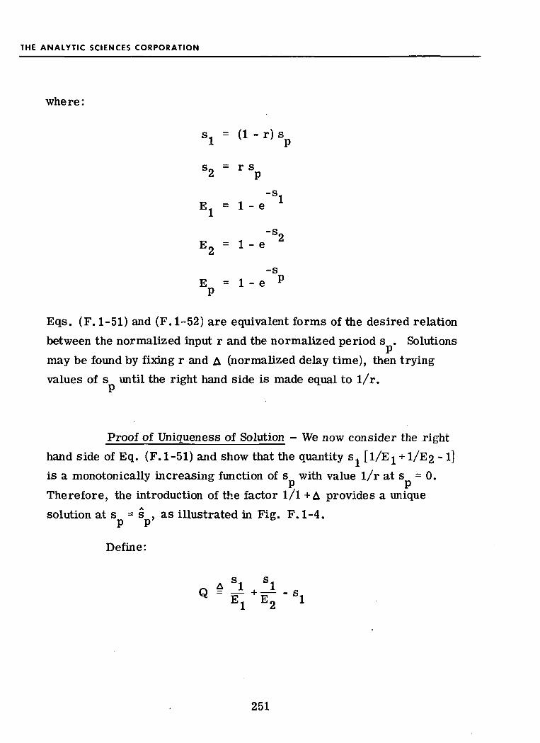
THE ANALYTIC SCIENCES CORPORATION
where:
Sl = ( 1 ' r ) sp
S2 = r Sp
E = 1 - e
~S2E2 = 1-e
-sE = 1-e p
Eqs. (F. 1-51) and (F. 1-52) are equivalent forms of the desired relation
between the normalized input r and the normalized period s . Solutions
may be found by fixing r and A (normalized delay time), then trying
values of s until the right hand side is made equal to 1/r.
Proof of Uniqueness of Solution - We now consider the right
hand side of Eq. (F. 1-51) and show that the quantity s. [l/E^ + 1/E2 - 1]
is a monotonically increasing function of s with value 1/r at s =0.
Therefore, the introduction of the factor 1/1 +A provides a unique
solution at s = s , as illustrated in Fig. F. 1-4.
Define:
A S1 S
2
251

THE ANALYTIC SCIENCES CORPORATION
K-2131
\
LL- 1
0 7UJQoo
QZ<Xh—XVon
Figure F. 1-4
NORMALIZED PERIOD,sp
Solution for Normalized Period
which is the right hand side of Eq. (F. 1-51) when A = 0. Clearly, thelimit of:
equals one (using L'Hospital's Rule) as s1 tends to zero. Similarly, thelimit of:
'1 _
252

THE ANALYTIC SCIENCES CORPORATION
equals (1 -r)/r as s tends to zero. Therefore:
lim Q = 1 + —- - 0 = -r r
This concludes the first part of the proof.
To prove that Q increases monotonically consider its
derivative :
j/-\/ _ dQ _- -1 -e
(F.l-53)
Q' is clearly positive for any s. if:
1^ "X0
e 2 I (for any x) (F.l-54)
253

THE ANALYTIC SCIENCES CORPORATION
Let:
-X -X
., -X -X1 - e - xe., o -x -2x1 -2e + e
., -x -x1 - e - xe
2 - 2e"x - 2xe"X - 1 + 2xe~x + e~2x
a2 a -
where:
We note that = 0 when x = 0. Furthermore:
(F.l-55)
- 2xe"X- e"2x (F.l-56)
dx
= [2e"X] [x- 1 -e"X] (F.l-57)
Both factors on the right hand side of Eq. (F. 1-57) are positive. Therefore:
( 3 ^ 0
R s 1/2
Q' s 0
254

THE ANALYTIC SCIENCES CORPORATION
and Q is monotonically increasing. This concludes the proof thatEq. (F. 1-51) or (F. 1-52) has a unique non-trivial solution for any non-zero values of r and A. Thus, there is one and only one oscillationperiod which satisfies the periodicity conditions for a given input leveland switching delay.
Comparison with Describing Function Analysis - A family ofsolutions to Eq. (F. 1-52) are plotted in Fig. F. 1-5. Note that the curvesare symmetrical about the mid-line, r = 0.5, and also exhibit minima(maximum frequencies of oscillation) at this point. This behavior wasillustrated in the example float angle histories pictured in Fig. F. 1-3.Note also that the curves are quite flat across a relatively wide mid-region, and that the period of oscillation appears to be proportional tothe square root of A. Inspection of the family of curves leads to thefollowing empirical formula, which is approximately correct in thismid-region:
* 7.0 /T = 7.0 J TD/r f ' (F.l-58)
Therefore:
P ^ 7.0 J r T (F.l-59)
We now compare Eq« (F0 1-59) with a result obtained using describingfunction analysis. The following formula for a limit cycle frequency ofoscillation in a binary or ternary rebalance loop was derived in Ref. 2.
TfTtg (F.l-60)
255

THE ANALYTIC SCIENCES CORPORATION
K -2132
zo
u</•>Ou_0
aO
UJa.
i
SEE SIMULATION RESULTPAGE 89, REF.3
0 0.25 Q5 0.75 1.0
RATIO OF INPUT TORQUE TO TORQUER CAPACITY,r=MQ/Mtg
Figure F. 1-5 Normalized Period Versus Normalized Input
This is the frequency at which the two linear loop elements cause acombined phase lag of TT radians. The corresponding period of oscillationis:
(Fol-61)
Eqs. (F. 1-59) and (F. 1-61) are nearly identical if the torque switchingdelay of the present model is equated with the torque generator timeconstant, r. . Note the point corresponding to A = 0.05 and r = 0.1
256

THE ANALYTIC SCIENCES CORPORATION
circled in Fig. F. 1-5. This point agrees very well with a simulated
response time history previously published in Ref. 3. The analysis
developed in this Appendix involves considerably more effort than des-
cribing function analysis, but it provides the ability to predict the varia-
tion in the oscillation period with input magnitude. Describing function
analysis cannot predict this type of result accurately because the input
to the nonlinearity is not very well represented by its fundamental com-
ponent alone in the case of small or large inputs to a ternary loop.
Derivation of Characteristic Amplitude - The previous analysis
can be extended in order to derive an expression for the peak-to-peak
amplitude of oscillation in the float angle. This amplitude is the difference
between the minimum float angle which occurs during the positive-torque
segment, and the maximum float angle, which occurs during the negative
torque segment. (Recall the assumption that the float angle does not go
too far in the "wrong" direction; there are no "wrong-way pulses.")
The minimum float angle occurs at normalized time, s . , whenminthe normalized rate of change, as given by Eq. (F01-29), equals zero.
Thus:
x' = x1'e"Smill+m1 (l-e"Smin) = 0 (F.l-62)
Therefore
-s6
257

THE ANALYTIC SCIENCES CORPORATION
and
s . =min (l - x ' /m. )\ 1 I/ (F.l-64)
Substitution of Eqs. (F. 1-63), (F01-64) and (F. 1-30) into Eq. (F. 1-28)
yields:
x . = 6 + x'min 1 A + 1 -
+ (F.l-65)
Similarly
max (F.l-66)
and:
x = 6 + x'max 2
+ m.
/x
- X (F.l-67)
Recalling that r = m. and -(1 -r) = m0, we can rewrite Eqs. (F.l-46) ini &the form:
X 'xl 1ml E*!
El "Sl( A \V 1+A/
= 1 - (F.l-68a)
258

THE ANALYTIC SCIENCES CORPORATION
Therefore:
where:
Also:
_E,
= 1 -
A1+A
E2(1+A)
Xl = ml
X2 =
S
w« =2 E2(1+A)
(F.l-68b)
(F.l-69a)
(F.l-69b)
1 / /— ~-~ A^ / J-H-f
1 - x2' /m2
1 TV1 /V '™ XXI / •*»>^
1 - m2 /x2'
= 1 - (
= 1 - (
_ i~ X " l
11 1
1 - W j
^1
-w l
1- w0
L J = W 1
j ) = W 21i
1 - 1/Wj
11 - l/w0
(F.,l-70a)
(F.l-70b)
(F.l-71a)
(F.l-71b)
259

THE ANALYTIC SCIENCES CORPORATION
Now, using the above relations in Eqs. (F.l-65) and (F. 1-67) we can
write for the peak-to-peak amplitude:
A x = x -x .pp max min
= 6 - (1 - r) (l - w2) FA + I - 1/wJ - (1 - r) fin wg- (l - l/w2)]
- 1/Wj)-6 - r l - W j A + l - l w - r
(F.l-72)
Simplifying, we obtain:
= r wr
(F.l-73)
Solutions to Eq. (F. 1-73) are plotted in Fig. F»l-6. These are
based on combinations of r, A and s. (normalized input, time delay and
positive torque interval) which were previously found to satisfy the
periodicity condition, Eq. (F. 1-52). The amplitude of oscillation appears
to be insensitive to input magnitude, even in the small and large input
regions where the frequency decreases markedly. Inspection of the
curves leads to the following empirical formula:
— s. 1.45 A = 1.45 — ' (F.l-74)> ^ T
260
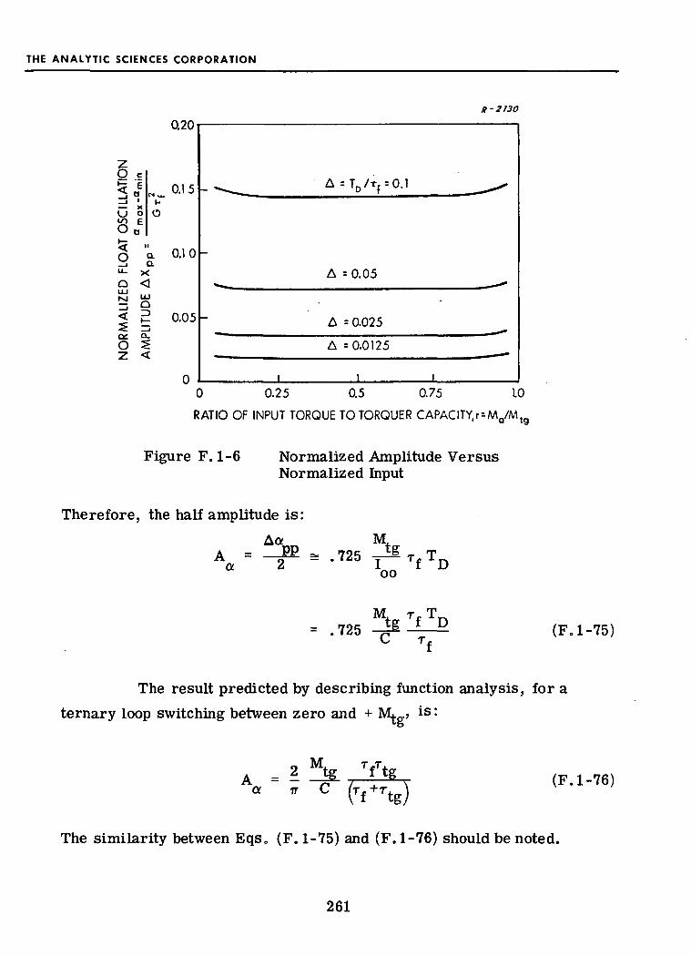
THE ANALYTIC SCIENCES CORPORATION
zo5id
X0h—<O_lu_
QLUM
1
<
5Q£O
Q20
c
J««. °-15
' ^o 0
Q
a 0.1 0Q.
X
<LU0
g 0.05— lex.5<
0
a -2 tso
_^_ A=T 0 / r f = 0.1 ^
-
A = 0.05
A = 0.025
A = 0.0125
i i i0 0.25 0.5 0.75 1.0
RATIO OF INPUT TORQUE TO TORQUER CAPACITY.r = MQ/Mtg
Figure F. 1-6 Normalized Amplitude VersusNormalized Input
Therefore, the half amplitude is:M
A =a.
^ .725oo
M
= .725T
f(F0l-75)
The result predicted by describing function analysis, for a
ternary loop switching between zero and + Mj._> is:
2 Mtg TfTtgIT (rf+rtg) (F.l-76)
The similarity between Eqs. (F. 1-75) and (F. 1-76) should be noted.
261

THE ANALYTIC SCIENCES CORPORATION
Summary - A convenient summary of all results for the
ternary rebalance loop is given in Fig. F. 1-7. In constructing this figure
we have accepted the describing function results in the vicinity of
r = ± 0.5 and used the preceding analysis to treat inputs of large andsmall magnitudes.
R-2128
zo
oQLLJ
OZ
oIUO£
1.0
0.5
1.0 -Q5 0 >0.5 +1.0
NORMALIZED INPUT MAGNITUDE.r=Ma/Mtg
zQ
_J—J
u °8 <\—
o
O)
iT
0
•"•"•?
K
^- in\? 1-vJ
u
Ollf
- u; 0.5Q Quj IDM- i—
< °-
»k* f
-
i l i I l l l-10 -05 0 >Q5 +1.0
NORMALIZED INPUT MAGNITUDE ,r = Ma/Mtg
Figure F.1-7 Summary of Results - Ternary Loop
262

THE ANALYTIC SCIENCES CORPORATION
F.2 ANALYSIS OF OSCILLATIONS IN THE BINARY LOOP
The analysis of ternary loop oscillations presented in thepreceding section may be applied directly to the binary loop» In thiscase the rebalance torque switches between + M, and - M. rather thantg tg+M. and zero. Therefore, the positive and negative net torque values,
respectively, are:
M = M - M. (F.2-2)02 a tg
After defining:
r = 0.5 + r/2
G = 2G = 2M, /Itg oo
we can write:
ml = M0 /!oo
= Mo /loo = -(1-?)6 (F-2'4'
The entire analysis then proceeds identically, except that r and G appear
in place of r and G. The non-dimensional results plotted in Figs. F. 1-5
and F. 1-6 are also correct if the abscissa is labeled r and the float angle** 9
excursion normalized by G rf .
263

THE ANALYTIC SCIENCES CORPORATION
The describing function results for the binary gyro with noinput (see Ref. 2) are:
ri Ttg (F'2"5)
These, again, agree with the plotted results in the mid-region, centeredaround r =0.5. However, the value r = 0. 5 corresponds to r = 0.Therefore, describing function theory accurately predicts binary loopbehavior in the region where the normalized input r is small. A con-venient summary of all results for the binary rebalance loop is given inFig. F.2-1. Comparison of Figs» F. 1-7 and F.2-1 shows that the des-cribing function technique is a good predictor of characteristic loopbehavior for half-maximum inputs (r == ± 0. 5) for ternary loops and forsmall inputs (r a« 0) for binary loops. Also, the factor-of-two differencein the amplitude normalizing quantities shows that, for the cases treatedby this analysis, the float angle oscillation amplitude is twice as largefor binary loops as for ternary loops.
264

THE ANALYTIC SCIENCES CORPORATION
8-2129
Zo
u8*°
o
o ^uj Zr-j uj
< O5 uj^ £o "•
S 1.0
0.5
-1.0 -0.5 0 0-5 1.0.
NORMALIZED INPUT MAGNITUDE,r=M0/M tg
ZQ
i
U w
<3<§
O)<r
1 "
£>5
"o.
i- 10t.
u
-I*8
- u; Q5
Q Quj ;DM |_~j i<; Q-5 S
-
1 1 1 1 1 1 1O < 10 05 0 0.5 l.(Z
NORMALIZED INPUT MAGNITUDE ,r = Ma/M tg
Figure F.2-1 Summary of Results - Binary Loop
265

Page Intentionally Left Blank

THE ANALYTIC SCIENCES CORPORATION
REFERENCES
1. Bumstead, R.M. and Vander Velde, W. E., "Navigation andGuidance Systems Employing a Gimballess IMU," AIAAPreprint No. 63-307, August 1963.
2. Gelb, Arthur, and Sutherland, Arthur A., Jr., "Design ofStrapdown Gyroscopes for a Dynamic Environment," TR-101-2,15 January 1968.
3. Sutherland, Arthur A., Jr., and Beebee, William S., "Designof Strapdown Gyroscopes for a Dynamic Environment," NASACR-1396, August 1969 (Also TR-101-4, January 1969).
4. Wimber, B.J., "The Apparent Input Axis Misalignment ErrorCaused by Angular Rotation about the Output Axis of a Single-Degree-of-Freedom, Rate-Integrating Gyro, "Fourth InertialGuidance Test Symposium Proceedings, MDC TR 68-76,November 1968.
5. Gelb, Arthur and Vander Velde, Wallace E., Multiple-InputDescribing Functions and Nonlinear System Design, McGraw-HillBook Co., August 1968.
6. Rauscher, M., Introduction to Aeronautical Dynamics, JohnWiley & Sons, New York, 1953.
7. Gelb, Arthur and Sutherland, Arthur A., Jr., "Application ofthe Kalman Filter to Aided Inertial Systems, " U.S. NavalWeapons Center, China Lake, California, NWC TP 4652,August 1968.
8. Bryson, A.E., and Ho, Y.C., Applied Optimal Control, BlaisdellCompany, Waltham, Massachusetts, 1969.
9. Hildebrand, F.B., Advanced Calculus for Engineers, PrenticeHall, New York, 1948.
10. Crawford, B.S., "Strapdown Sensor Tests and Test DataAnalysis," TR-147-1, 31 January 1970.
267
