Analysis of the Binary Instrumental Variable Model

Thomas S. Richardson

University of Washington

James M. Robins

Harvard School of Public Health

Working Paper no. 99

Center for Statistics and the Social Sciences

University of Washington

29 March, 2010

Abstract

We give an explicit geometric characterization of the set of distributions over counterfactuals

that are compatible with a given observed joint distribution for the observables in the binary

instrumental variable model.

This paper will appear as Chapter 25 in Heuristics, Probability and Causality: A Tribute to

Judea Pearl. R. Dechter, H. Geffner and J.Y. Halpern, Editors, College Publications, UK.

1 Introduction

Pearl’s seminal work on instrumental variables [Chickering and Pearl 1996; Balke and Pearl

1997] for discrete data represented a leap forwards in terms of understanding: Pearl showed

that, contrary to what many had supposed based on linear models, in the discrete case

the assumption that a variable was an instrument could be subjected to empirical test. In

addition, Pearl improved on earlier bounds [Robins 1989] for the average causal effect (ACE)

in the absence of any monotonicity assumptions. Pearl’s approach was also innovative insofar

as he employed a computer algebra system to derive analytic expressions for the upper and

lower bounds.

In this paper we build on and extend Pearl’s work in two ways. First we show the

geometry underlying Pearl’s bounds. As a consequence we are able to derive bounds on

the average causal effect for all four compliance types. Our analysis also makes it possible

to perform a sensitivity analysis using the distribution over compliance types. Second our

analysis provides a clear geometric picture of the instrumental inequalities, and allows us

to isolate the counterfactual assumptions necessary for deriving these tests. This may be

seen as analogous to the geometric study of models for two-way tables [Fienberg and Gilbert

1970; Erosheva 2005]. Among other things this allows us to clarify which are the alternative

hypotheses against which Pearl’s test has power. We also relate these tests to recent work

of Pearl’s on bounding direct effects [Cai, Kuroki, Pearl, and Tian 2008].

2 Background

We consider three binary variables, X, Y and Z. Where:

Z is the instrument, presumed to be randomized e.g. the assigned treatment;

X is the treatment received;

Y is the response.

For X and Z, we will use 0 to indicate placebo, and 1 to indicate drug. For Y we take

1 to indicate a desirable outcome, such as survival. Xz is the treatment a patient would

receive if assigned to Z = z. We follow convention by referring to the four compliance types:

1

tX , tY

Z X Y

Figure 1: Graphical representation of the IV model given by assumptions (1) and (2).The

shaded nodes are observed.

Xz=0 Xz=1 Compliance Type

0 0 Never Taker NT

0 1 Complier CO

1 0 Defier DE

1 1 Always Taker AT

Since we suppose the counterfactuals are well-defined, if Z = z then X = Xz. Similarly

we consider counterfactuals Yxz for Y . Except where explicitly noted we will make the

exclusion restrictions:

Yx=0,z=0 = Yx=0,z=1 Yx=1,z=0 = Yx=1,z=1 (1)

for each patient, so that a patient’s outcome only depends on treatment assigned via the

treatment received. One consequence of the analysis below is that these equations may be

tested separately. We may thus similarly enumerate four types of patient in terms of their

response to received treatment:

Yx=0 Yx=1 Response Type

0 0 Never Recover NR

0 1 Helped HE

1 0 Hurt HU

1 1 Always Recover AR

As before, it is implicit in our notation that if X = x, then Yx = Y ; this is referred to as the

‘consistency assumption’ (or axiom) by Pearl among others. In what follows we will use tX

to denote a generic compliance type in the set DX , and tY to denote a generic response type

in the set DY . We thus have 16 patient types:

〈tX , tY 〉 ∈ {NT, CO, DE, AT}× {NR, HE, HU, AR} ≡ DX × DY ≡ D.

(Here and elsewhere we use angle brackets 〈tX , tY 〉 to indicate an ordered pair.) Let πtX≡

p(tX) denote the marginal probability of a given compliance type tX ∈ DX , and let

πX ≡ {πtX| tX ∈ DX}

2

denote a marginal distribution on DX . Similarly we use πtY |tX≡ p(tY | tX) to denote the

probability of a given response type within the sub-population of individuals of compliance

type tX , and πY |X to indicate a specification of all these conditional probabilities:

πY |X ≡ {πtY |tX| tX ∈ DX , tY ∈ DY }.

We will use π to indicate a joint distribution p(tX , tY ) on D.

Except where explicitly noted we will make the randomization assumption that the dis-

tribution of types 〈tX , tY 〉 is the same in both arms:

Z ⊥⊥ {Xz=0, Xz=1, Yx=0, Yx=1}. (2)

A graph corresponding to the model given by (1) and (2) is shown in Figure 1.

2.0.1 Notation

In places we will make use of the following compact notation for probability distributions:

pyk|xjzi≡ p(Y = k | X = j, Z = i),

pxj |zi≡ p(X = j | Z = i),

pykxj |zi≡ p(Y = k, X = j | Z = i).

There are several simple geometric constructions that we will use repeatedly. In conse-

quence we introduce these in a generic setting.

2.1 Joints compatible with fixed margins

Consider a bivariate random variable U = 〈U1, U2〉 ∈ {0, 1}× {0, 1}. Now for fixed c1, c2 ∈

[0, 1] consider the set

Pc1,c2 =

{

p

∣

∣

∣

∣

∣

∑

u2

p(1, u2) = c1 ;∑

u1

p(u1, 1) = c2

}

in other words, Pc1,c2 is the set of joint distributions on U compatible with fixed margins

p(Ui = 1) = ci, i = 1, 2.

It is not hard to see that Pc1,c2 is a one-dimensional subset (line segment) of the 3-

dimensional simplex of distributions for U . We may describe it explicitly as follows:

p(1, 1) = t

p(1, 0) = c1 − t

p(0, 1) = c2 − t

p(0, 0) = 1 − c1 − c2 + t

t ∈[

max {0, (c1 + c2) − 1} , min {c1, c2}]

. (3)

3

c1

c2

0 1

1

(iii)

(i)

(ii)

(iv)

Figure 2: The four regions corresponding to different supports for t in (3); see Table 1.

See also [Pearl 2000] Theorem 9.2.10. The range of t, or equivalently the support for p(1, 1),

is one of four intervals, as shown in Table 1. These cases correspond to the four regions show

c1 ≤ 1 − c2 c1 ≥ 1 − c2

c1 ≤ c2 (i) t ∈ [0, c1] (ii) t ∈ [c1 + c2 − 1, c1]

c1 ≥ c2 (iii) t ∈ [0, c2] (iv) t ∈ [c1 + c2 − 1, c2]

Table 1: The support for t in (3) in each of the four cases relating c1 and c2.

in Figure 2.

Finally, we note that since for c1, c2 ∈ [0, 1], max {0, (c1 + c2) − 1} ≤ min {c1, c2}, it

follows that {〈c1, c2〉 | Pc1,c2 *= ∅} = [0, 1]2. Thus for every pair of values 〈c1, c2〉 there exists

a joint distribution p(U1, U2) for which p(Ui = 1) = ci, i = 1, 2.

2.2 Two quantities with a specified average

We now consider the set:

Qc,α = {〈u, v〉 | αu + (1 − α)v = c, u, v ∈ [0, 1]}

where c, α ∈ [0, 1]. In words, Qc,α is the set of pairs of values 〈u, v〉 in [0, 1] which are such

that the weighted average αu + (1 − α)v is c.

It is simple to see that this describes a line segment in the unit square. Further consid-

eration shows that for any value of α ∈ [0, 1], the segment will pass through the point 〈c, c〉

and will be contained within the union of two rectangles:

([c, 1] × [0, c]) ∪ ([0, c] × [1, c]).

4

u

v

0 1

1

c

c

Figure 3: Illustration of Qc,α.

The slope of the line is negative for α ∈ (0, 1). For α ∈ (0, 1) the line segment may be

parametrized as follows:{

u = (c − t(1 − α))/α,

v = t,t ∈

[

max

(

0,c − α

1 − α

)

, min

(

c

1 − α, 1

)]

}

.

The left and right endpoints of the line segment are:

〈u, v〉 =

⟨

max(

0, 1 + (c − 1)/α)

, min(

c/(1 − α), 1)

⟩

and

〈u, v〉 =

⟨

min(

c/α, 1)

, max(

0, (c − α)/(1 − α))

⟩

respectively. See Figure 3.

2.3 Three quantities with two averages specified

We now extend the discussion in the previous section to consider the set:

Q(c1,α1)(c2,α2) = {〈u, v, w〉 | α1u + (1 − α1)w = c1,

α2v + (1 − α2)w = c2, u, v, w ∈ [0, 1]} .

In words, this consists of the set of triples 〈u, v, w〉 ∈ [0, 1]3 for which pre-specified averages

of u and w (via α1), and v and w (via α2) are equal to c1 and c2 respectively.

If this set is not empty, it is a line segment in [0, 1]3 obtained by the intersection of two

rectangles:(

{〈u, w〉 ∈ Qc1,α1}× {v ∈ [0, 1]}

)

∩

(

{〈v, w〉 ∈ Qc2,α2}× {u ∈ [0, 1]}

)

; (4)

see Figures 4 and 5. For α1, α2 ∈ (0, 1) we may parametrize the line segment (4) as follows:

5

Figure 4: (a) The plane without stripes is α1u + (1 − α1)w = c1. (b) The plane without

checks is α2v + (1 − α2)w = c2.

u = (c1 − t(1 − α1))/α1,

v = (c2 − t(1 − α2))/α2,

w = t,

t ∈ [tl, tu]

,

where

tl ≡ max

{

0,c1 − α1

1 − α1,c2 − α2

1 − α2

}

, tu ≡ min

{

1,c1

1 − α1,

c2

1 − α2

}

.

Thus Q(c1,α1)(c2,α2) *= ∅ if and only if tl ≤ tu. It follows directly that for fixed c1, c2 the

set of pairs 〈α1, α2〉 ∈ [0, 1]2 for which Q(c1,α1)(c2,α2) is not empty may be characterized thus:

Rc1,c2 ≡{

〈α1, α2〉∣

∣Q(c1,α1)(c2,α2) *= ∅}

= [0, 1]2 ∩⋂

i∈{1,2}

i∗=3−i

{〈α1, α2〉 | (αi − ci)(αi∗ − (1 − ci∗)) ≤ c∗i (1 − ci)}. (5)

In fact, as shown in Figure 6 at most one constraint is active, so simplification is possible:

let k = arg maxj cj , and k∗ = 3 − k, then

Rc1,c2 = [0, 1]2 ∩ {〈α1, α2〉 | (αk − ck)(αk∗ − (1 − ck∗)) ≤ c∗k(1 − ck)}.

(If c1 = c2 then Rc1,c2 = [0, 1]2.)

In the two dimensional analysis in §2.2 we observed that for fixed c, as α varied, the

line segment would always remain inside two rectangles, as shown in Figure 3. In the three

dimensional situation, the line segment (4) will stay within three boxes:

6

Figure 5: Q(c1,α1)(c2,α2) corresponds to the section of the line between the two marked points;

(a) view towards u-w plane; (b) view from v-w plane. (Here c1 < c2.)

(i) If c1 < c2 then the line segment (4) is within:

([0, c1] × [0, c2] × [c2, 1]) ∪ ([0, c1] × [c2, 1] × [c1, c2]) ∪ ([c1, 1] × [c2, 1] × [0, c1]).

This may be seen as a ‘staircase’ with a ‘corner’ consisting of three blocks, descending

clockwise from 〈0, 0, 1〉 to 〈1, 1, 0〉; see Figure 7(a). The first and second boxes intersect

in the line segment joining the points 〈0, c2, c2〉 and 〈c1, c2, c2〉; the second and third

intersect in the line segment joining 〈c1, c2, c1〉 and 〈c1, 1, c1〉.

(ii) If c1 > c2 then the line segment is within:

([0, c1] × [0, c2] × [c1, 1]) ∪ ([c1, 1] × [0, c2] × [c2, c1]) ∪ ([c1, 1] × [c2, 1] × [0, c2]).

This is a ‘staircase’ of three blocks, descending counter-clockwise from 〈0, 0, 1〉 to

〈1, 1, 0〉; see Figure 7(b). The first and second boxes intersect in the line segment

joining the points 〈c1, 0, c1〉 and 〈c1, c2, c1〉; the second and third intersect in the line

segment joining 〈c1, c2, c2〉 and 〈1, c2, c2〉.

(iii) If c1 = c2 = c then the ‘middle’ box disappears and we are left with

([0, c] × [0, c] × [c, 1]) ∪ ([c, 1] × [c, 1] × [0, c]).

In this case the two boxes touch at the point 〈c, c, c〉.

Note however, that the number of ‘boxes’ within which the line segment (4) lies may be 1,

2 or 3 (or 0 if Q(c1,α1)(c2,α2) = ∅). This is in contrast to the simpler case considered in §2.2

where the line segment Qc,α always intersected exactly two rectangles; see Figure 3.

7

Figure 6: Rc1,c2 corresponds to the shaded region. The hyperbola of which one arm forms

a boundary of this region corresponds to the active constraint; the other hyperbola to the

inactive constraint.

3 Characterization of compatible distributions of type

Returning to the Instrumental Variable model introduced in §2, for a given patient the

values taken by Y and X are deterministic functions of Z, tX and tY . Consequently, under

randomization (2), a distribution over D determines the conditional distributions p(x, y | z)

for z ∈ {0, 1}. However, since distributions on D form a 15 dimensional simplex, while

p(x, y | z) is of dimension 6, it is clear that the reverse does not hold; thus many different

distributions over D give rise to the same distributions p(x, y | z). In what follows we

precisely characterize the set of distributions over D corresponding to a given distribution

p(x, y | z).

We will accomplish this in the following steps:

1. We first characterize the set of distributions πX on DX compatible with a given distri-

bution p(x | z).

2. Next we use the technique used for Step 1 to reduce the problem of characterizing

distributions πY |X compatible with p(x, y | z) to that of characterizing the values of

p(yx = 1 | tX) compatible with p(x, y | z).

3. For a fixed marginal distribution πX on DX we then describe the set of values for

p(yx = 1 | x, tX) compatible with the observed distribution p(y | x, z).

4. In general, some distributions πX on DX and observed distributions p(y | x, z) may be

incompatible in that there are no compatible values for p(yx = 1 | tX). We use this to

find the set of distributions πX on DX compatible with p(y, x | z) (by restricting the

set of distributions found at step 1).

8

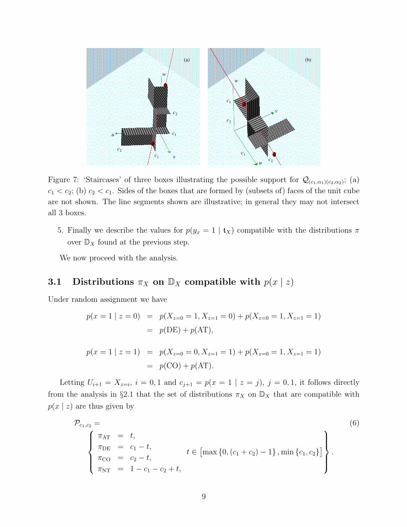
Figure 7: ‘Staircases’ of three boxes illustrating the possible support for Q(c1,α1)(c2,α2); (a)

c1 < c2; (b) c2 < c1. Sides of the boxes that are formed by (subsets of) faces of the unit cube

are not shown. The line segments shown are illustrative; in general they may not intersect

all 3 boxes.

5. Finally we describe the values for p(yx = 1 | tX) compatible with the distributions π

over DX found at the previous step.

We now proceed with the analysis.

3.1 Distributions πX on DX compatible with p(x | z)

Under random assignment we have

p(x = 1 | z = 0) = p(Xz=0 = 1, Xz=1 = 0) + p(Xz=0 = 1, Xz=1 = 1)

= p(DE) + p(AT),

p(x = 1 | z = 1) = p(Xz=0 = 0, Xz=1 = 1) + p(Xz=0 = 1, Xz=1 = 1)

= p(CO) + p(AT).

Letting Ui+1 = Xz=i, i = 0, 1 and cj+1 = p(x = 1 | z = j), j = 0, 1, it follows directly

from the analysis in §2.1 that the set of distributions πX on DX that are compatible with

p(x | z) are thus given by

Pc1,c2 = (6)

πAT = t,

πDE = c1 − t,

πCO = c2 − t,

πNT = 1 − c1 − c2 + t,

t ∈[

max {0, (c1 + c2) − 1} , min {c1, c2}]

.

9

p(AR | tX)

p(HE | tX) p(HU | tX)

p(NR | tX)

γ1

tX

γ0

tX

1

Figure 8: A graph representing the functional dependencies used in the reduction step in

§3.2. The rectangular node indicates that the probabilities are required to sum to 1.

3.2 Reduction step in characterizing distributions πY |X compatible

with p(x, y | z)

Suppose that we were able to ascertain the set of possible values for the eight quantities:

γitX

≡ p(yx=i = 1 | tX), for i ∈ {0, 1} and tX ∈ DX ,

that are compatible with p(x, y | z). Note that p(yx=i = 1 | tX) is written as p(y = 1 | do(x=

i), tX) using Pearl’s do(·) notation. It is then clear that the set of possible distributions πY |X

that are compatible with p(x, y | z) simply follows from the analysis in §2.1, since

γ0tX

= p(yx=0 = 1 | tX)

= p(HU | tX) + p(AR | tX),

γ1tX

= p(yx=1 = 1 | tX)

= p(HE | tX) + p(AR | tX).

These relationships are also displayed graphically in Figure 8: in this particular graph all

children are simple sums of their parents; the boxed 1 represents the ‘sum to 1’ constraint.

Thus, by §2.1, for given values of γitX

the set of distributions πY |X is given by:

p(AR | tX) ∈[

max{

0, (γ0tX

+ γ1tX

) − 1}

, min{

γ0tX

, γ1tX

}]

,

p(NR | tX) = 1 − γ0tX

− γ1tX

+ p(AR | tX),

p(HE | tX) = γ1tX

− p(AR | tX),

p(HU | tX) = γ0tX

− p(AR | tX)

. (7)

It follows from the discussion at the end of §2.1 that the values of γ0tX

and γ1tX

are not

restricted by the requirement that there exists a distribution p(· | tX) on DY . Consequently

10

γ0AT

γ0NT

πX γ1NT

γ1AT

p(y|x=0, z=1) p(x|z=1) p(y|x=1, z=1)

p(y|x=0, z=0) p(x|z=0) p(y|x=1, z=0)

γ0CO

γ1DE

γ0DE

γ1CO

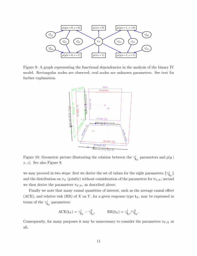
Figure 9: A graph representing the functional dependencies in the analysis of the binary IV

model. Rectangular nodes are observed; oval nodes are unknown parameters. See text for

further explanation.

Figure 10: Geometric picture illustrating the relation between the γitX

parameters and p(y |

x, z). See also Figure 9.

we may proceed in two steps: first we derive the set of values for the eight parameters {γitX}

and the distribution on πX (jointly) without consideration of the parameters for πY |X ; second

we then derive the parameters πY |X, as described above.

Finally we note that many causal quantities of interest, such as the average causal effect

(ACE), and relative risk (RR) of X on Y , for a given response type tX , may be expressed in

terms of the γitX

parameters:

ACE(tX) = γ1tX

− γ0tX

, RR(tX) = γ1tX

/γ0tX

.

Consequently, for many purposes it may be unnecessary to consider the parameters πY |X at

all.

11

3.3 Values for {γi

tX

} compatible with πX and p(y | x, z)

We will call a specification of values for πX, feasible for the observed distribution if (a) πX

lies within the set described in §3.1 of distributions compatible with p(x | z) and (b) there

exists a set of values for γitX

which results in the distribution p(y | x, z).

In the next section we give an explicit characterization of the set of feasible distributions

πX ; in this section we characterize the set of values of γitX

compatible with a fixed feasible

distribution πX and p(y | x, z).

Proposition 1 The following equations relate πX , γ0CO, γ0

DE, γ0NT to p(y | x=0, z):

p(y=1 | x=0, z=0) = (γ0COπCO + γ0

NTπNT)/(πCO + πNT), (8)

p(y=1 | x=0, z=1) = (γ0DEπDE + γ0

NTπNT)/(πDE + πNT), (9)

Similarly, the following relate πX , γ1CO, γ1

DE, γ1AT to p(y | x=1, z):

p(y=1 | x=1, z=0) = (γ1DEπDE + γ1

ATπAT)/(πDE + πAT), (10)

p(y=1 | x=1, z=1) = (γ1COπCO + γ1

ATπAT)/(πCO + πAT). (11)

Equations (8)–(11) are represented in Figure 9. Note that the parameters γ0AT and γ1

NT

are completely unconstrained by the observed distribution since they describe, respectively,

the effect of non-exposure (X = 0) on Always Takers, and exposure (X = 1) on Never

Takers, neither of which ever occur. Consequently, the set of possible values for each of

these parameters is always [0, 1]. Graphically this corresponds to the disconnection of γ0AT

and γ1NT from the remainder of the graph.

As shown in Proposition 1 the remaining six parameters may be divided into two groups,

{γ0NT, γ0

DE, γ0CO} and {γ1

AT, γ1DE, γ1

CO}, depending on whether they relate to unexposed sub-

jects, or exposed subjects. Furthermore, as the graph indicates, for a fixed feasible value of

πX , compatible with the observed distribution p(x, y | z) (assuming such exists), these two

sets are variation independent. Thus, for a fixed feasible value of πX we may analyze each

of these sets separately.

A geometric picture of equations (8)–(11) is given in Figure 10: there is one square for

each compliance type, with axes corresponding to γ0tX

and γ1tX

; the specific value of 〈γ0tX

, γ1tX〉

is given by a cross in the square. There are four lines corresponding to the four observed

quantities p(y = 1 | x, z). Each of these observed quantities, which is denoted by a cross on

the respective line, is a weighted average of two γitX

parameters, with weights given by πX

(the weights are not depicted explicitly).

12

Proof of Proposition 1: We prove (8); the other proofs are similar. Subjects for whom X = 0

and Z = 0 are either Never Takers or Compliers. Hence

p(y=1 | x=0, z=0) = p(y=1 | x=0, z=0, tX =NT)p(tX =NT | x=0, z=0)

+p(y=1 | x=0, z=0, tX =CO)p(tX =CO | x=0, z=0)

= p(yx=0=1 | x=0, z=0, tX =NT)p(tX =NT | tX ∈ {CO, NT})

+p(yx=0 =1 | x=0, z=0, tX =CO)p(tX =CO | tX ∈ {CO, NT})

= p(yx=0=1 | z=0, tX =NT) × πNT/(πNT + πCO)

+p(yx=0 =1 | z=0, tX =CO) × πCO/(πNT + πCO)

= p(yx=0=1 | tX =NT) × πNT/(πNT + πCO)

+p(yx=0 =1 | tX =CO) × πCO/(πNT + πCO)

= (γ0COπCO + γ0

NTπNT)/(πCO + πNT).

Here the first equality is by the chain rule of probability; the second follows by consistency;

the third follows since Compliers and Never Takers have X = 0 when Z = 0; the fourth

follows by randomization (2). !

Values for γ0CO, γ0

DE, γ0NT compatible with a feasible πX

Since (8) and (9) correspond to three quantities with two averages specified, we may apply

the analysis in §2.3, taking α1 = πCO/(πCO +πNT), α2 = πDE/(πDE +πNT), ci = p(y=1 | x=

0, z= i − 1) for i = 1, 2, u = γ0CO, v = γ0

DE and w = γ0NT. Under this substitution, the set of

possible values for 〈γ0CO, γ0

DE, γ0NT〉 is then given by Q(c1,α1)(c2,α2).

Values for γ1CO, γ1

DE, γ1AT compatible with a feasible πX

Likewise since (10) and (11) contain three quantities with two averages specified we again

apply the analysis from §2.3, taking α1 = πCO/(πCO + πAT), α2 = πDE/(πDE + πAT), ci =

p(y = 1 | x = 1, z = 2 − i) for i = 1, 2, u = γ1CO, v = γ1

DE and w = γ1AT. The set of possible

values for 〈γ1CO, γ1

DE, γ1AT〉 is then given by Q(c1,α1)(c2,α2).

3.4 Values of πX compatible with p(x, y | z)

In §3.1 we characterized the distributions πX compatible with p(x | z) as a one dimensional

subspace of the three dimensional simplex, parameterized in terms of t ≡ πAT; see (6). We

now incorporate the additional constraints on πX that arise from p(y | x, z). These occur

13

because some distributions πX , though compatible with p(x | z), lead to an empty set of

values for 〈γ1CO, γ1

DE, γ1AT〉 or 〈γ0

CO, γ0DE, γ0

NT〉 and thus are infeasible.

3.4.1 Constraints on πX arising from p(y | x = 0, z)

Building on the analysis in §3.3 the set of values for

〈α1, α2〉 = 〈πCO/(πCO + πNT), πDE/(πDE + πNT)〉

= 〈πCO/px0|z0, πDE/px0|z0

〉 (12)

compatible with p(y | x=0, z) (i.e. for which the corresponding set of values for 〈γ0CO, γ0

DE, γ0NT〉

is non-empty) is given by Rc∗1,c∗

2, where c∗i = p(y = 1 | x = 0, z = i − 1), i = 1, 2 (see §2.3).

The inequalities defining Rc∗1,c∗

2may be translated into upper bounds on t ≡ πAT in (6), as

follows:

t ≤ min

1 −∑

j∈{0,1}

p(y=j, x=0 | z=j), 1 −∑

k∈{0,1}

p(y=k, x=0 | z=1−k)

. (13)

Proof: The analysis in §3.3 implied that for Rc∗1,c∗

2*= ∅ we require

c∗1 − α1

1 − α1≤

c∗21 − α2

andc∗2 − α2

1 − α2≤

c∗11 − α1

. (14)

Taking the first of these and plugging in the definitions of c∗1, c∗2, α1 and α2 from (12) gives:

py1|x0,z0− (πCO/px0|z0

)

1 − (πCO/px0|z0)

≤py1|x0,z1

1 − (πDE/px0|z1)

(⇔) (py1|x0,z0− (πCO/px0|z0

))(1 − (πDE/px0|z1)) ≤ py1|x0,z1

(1 − (πCO/px0|z0))

(⇔) (py1,x0|z0− πCO)(px0|z1

− πDE) ≤ py1,x0|z1(px0|z0

− πCO).

But px0|z1− πDE = px0|z0

− πCO = πNT, hence these terms may be cancelled to give:

(py1,x0|z0− πCO) ≤ py1,x0|z1

(⇔) πAT − px1|z1≤ py1,x0|z1

− py1,x0|z0

(⇔) πAT ≤ 1 − py0,x0|z1− py1,x0|z0

.

A similar argument applied to the second constraint in (14) to derive that

πAT ≤ 1 − py0,x0|z0− py1,x0|z1

,

as required. !

14

3.4.2 Constraints on πX arising from p(y | x = 1, z)

Similarly using the analysis in §3.3 the set of values for

〈α1, α2〉 = 〈πCO/(πCO + πAT), πDE/(πDE + πAT)〉

compatible with p(y | x=1, z) (i.e. that the corresponding set of values for 〈γ1CO, γ1

DE, γ1AT〉

is non-empty) is given by Rc∗∗1

,c∗∗2

, where c∗∗i = p(y = 1 | x = 1, z = 2 − i), i = 1, 2 (see

§2.3). Again, we translate the inequalities which define Rc∗∗1

,c∗∗2

into further upper bounds

on t = πAT in (6):

t ≤ min

∑

j∈{0,1}

p(y=j, x=1 | z=j),∑

k∈{0,1}

p(y=k, x=1 | z=1−k)

. (15)

The proof that these inequalities are implied, is very similar to the derivation of the upper

bounds on πAT arising from p(y | x = 0, z) considered above.

3.4.3 The distributions πX compatible with the observed distribution

It follows that the set of distributions on DX that are compatible with the observed distri-

bution, which we denote PX , may be given thus:

PX =

πAT ∈ [lπAT, uπAT],

πNT(πAT) = 1 − p(x = 1 | z = 0) − p(x = 1 | z = 1) + πAT,

πCO(πAT) = p(x = 1 | z = 1) − πAT,

πDE(πAT) = p(x = 1 | z = 0) − πAT

, (16)

where

lπAT = max {0, p(x = 1 | z = 0) + p(x = 1 | z = 1) − 1} ;

uπAT = min

p(x = 1 | z = 0), p(x = 1 | z = 1),

1 −∑

j p(y=j, x=0 | z=j), 1 −∑

k p(y=k, x=0 | z=1−k),∑

j p(y=j, x=1 | z=j),∑

k p(y=k, x=1 | z=1−k)

.

Observe that unlike the upper bound, the lower bound on πAT (and πNT) obtained from

p(x, y | z) is the same as the lower bound derived from p(x | z) alone.

We define πX(πAT) ≡ 〈πNT(πAT), πCO(πAT), πDE(πAT), πAT〉, for use below. Note the follow-

ing:

Proposition 2 When πAT (equivalently πNT) is minimized then either πNT = 0 or πAT = 0.

Proof: This follows because, by the expression for lπAT, either lπAT = 0, or lπAT = p(x = 1 |

z = 0) + p(x = 1 | z = 1) − 1, in which case lπNT = 0 by (16). !

15

4 Projections

The analysis in §3 provides a complete description of the set of distributions over D com-

patible with a given observed distribution. In particular, equation (16) describes the one

dimensional set of compatible distributions over DX ; in §3.3 we first gave a description of the

one dimensional set of values over 〈γ0CO, γ0

DE, γ0NT〉 compatible with the observed distribution

and a specific feasible distribution πX over DX ; we then described the one dimensional set

of values for 〈γ1CO, γ1

DE, γ1AT〉. Varying πX over the set PX of feasible distributions over DX ,

describes a set of lines, forming two two-dimensional manifolds which represent the space of

possible values for 〈γ0CO, γ0

DE, γ0NT〉 and likewise for 〈γ1

CO, γ1DE, γ1

AT〉. As noted previously, the

parameters γ0AT and γ1

NT are unconstrained by the observed data. Finally, if there is inter-

est in distributions over response types, there is a one-dimensional set of such distributions

associated with each possible pair of values from γ0tX

and γ1tX

.

For the purposes of visualization it is useful to look at projections. There are many such

projections that could be considered, here we focus on projections that display the relation

between the possible values for πX and γxtX

. See Figure 11.

We make the following definition:

αij

tX(πX) ≡ p(tX | Xz=i = j),

where πX = 〈πNT, πCO, πDE, πAT〉 ∈ PX , as before. For example, α00NT(πX) = πNT/(πNT +

πCO), α10NT(πX) = πNT/(πNT + πDE).

4.1 Upper and Lower bounds on γx

tX

as a function of πX

We use the following notation to refer to the upper and lower bounds on γ0NT and γ1

AT that

were derived earlier. If πX is such that πNT > 0, so α00NT

, α10NT

> 0 then we define:

lγ0NT(πX) ≡ max

{

0,py1|x0z0

− α00CO

(πX)

α00NT

(πX),py1|x0z1

− α10DE

(πX)

α10NT

(πX)

}

,

uγ0NT(πX) ≡ min

{

py1|x0z0

α00NT

(πX),

py1|x0z1

α10NT

(πX), 1

}

,

while if πNT = 0 then we define lγ0NT(πX) ≡ 0 and uγ0

NT(πX) ≡ 1. Similarly, if πX is such

that πAT > 0 then we define:

lγ1AT(πX) ≡ max

{

0,py1|x1z1

− α11CO

(πX)

α11AT

(πX),py1|x1z0

− α01DE

(πX)

α01AT

(πX)

}

,

uγ1AT(πX) ≡ min

{

py1|x1z1

α11AT

(πX),

py1|x1z0

α01AT

(πX), 1

}

,

16

Lower Bound Upper Bound

γ0NT lγ0

NT(πX) uγ0NT(πX)

γ0CO (py1|x0z0

− uγ0NT(πX) · α00

NT)/α00

CO(py1|x0z0

− lγ0NT(πX) · α00

NT)/α00

CO

γ0DE (py1|x0z1

− uγ0NT(πX) · α10

NT)/α10

DE(py1|x0z1

− lγ0NT(πX) · α10

NT)/α10

DE

γ0AT 0 1

γ1NT 0 1

γ1CO (py1|x1z1

− uγ1AT(πX) · α11

AT)/α11

CO(py1|x1z1

− lγ1AT(πX) · α11

AT)/α11

CO

γ1DE (py1|x1z0

− uγ1AT(πX) · α01

AT)/α01

DE(py1|x1z0

− lγ1AT(πX) · α01

AT)/α01

DE

γ1AT lγ1

AT(πX) uγ1AT(πX)

Table 2: Upper and Lower bounds on γxtX

, as a function of πX ∈ PX . If for some πX

an expression giving a lower bound for a quantity is undefined then the lower bound is 0;

conversely if an expression for an upper bound is undefined then the upper bound is 1.

while if πAT = 0 then let lγ1AT(πX) ≡ 0 and uγ1

AT(πX) ≡ 1.

We note that Table 2 summarizes the upper and lower bounds, as a function of πX ∈ PX ,

on each of the eight parameters γxtX

that were derived earlier in §3.3. These are shown by

the thicker lines on each of the plots forming the upper and lower boundaries in Figure 11

(γ0AT and γ1

NT are not shown in the Figure).

The upper and lower bounds on γ0NT and γ1

AT are relatively simple:

Proposition 3 lγ0NT(πX) and lγ1

AT(πX) are non-decreasing in πAT and πNT. Likewise uγ0NT(πX)

and uγ1AT(πX) are non-increasing in πAT and πNT.

Proof: We first consider lγ0NT. By (16), πNT = 1 − p(x = 1 | z = 0) − p(x = 1 | z =

1) + πAT, hence a function is non-increasing [non-decreasing] in πAT iff it is non-increasing

[non-decreasing] in πNT. Observe that for πNT > 0,

(py1|x0z0− α00

CO(πX))/α00

NT(πX) =

(

py1|x0z0(πNT + πCO) − πCO

)

/πNT

= py1|x0z0− py0|x0z0

(πCO/πNT)

= py1|x0z0+ py0|x0z0

(1 − (px0|z0/πNT))

which is non-decreasing in πNT. Similarly,

(py1|x0z1− α10

DE(πX))/α10

NT(πX) = py1|x0z1

+ py0|x0z1(1 − (px0|z1

/πNT)).

17

The conclusion follows since the maximum of a set of non-decreasing functions is non-

decreasing.

The other arguments are similar. !

We note that the bounds on γxCO and γx

DE need not be monotonic in πAT.

Proposition 4 Let πminX be the distribution in PX for which πAT and πNT are minimized

then either:

(1) πminNT = 0, hence lγ0

NT(πminX ) = 0 and uγ0

NT(πminX ) = 1; or

(2) πminAT = 0, hence lγ1

AT(πminX ) = 0 and uγ1

AT(πminX ) = 1.

Proof: This follows from Proposition 2, and the fact that if πtX= 0 then γi

tXis not identified

(for any i). !

4.2 Upper and Lower bounds on p(AT) as a function of γ0NT

The expressions given in Table 2 allow the range of values for each γitX

to be determined

as a function of πX , giving the upper and lower bounding curves in Figure 11. However it

follows directly from (8) and (9) that there is a bijection between the three shapes shown

for γ0CO, γ0

DE and γ0NT (top row of Figure 11). In this section we describe this bijection by

deriving curves corresponding to fixed values of γ0NT that are displayed in the plots for γ0

CO

and γ0DE. Similarly it follows from (10) and (11) that there is a bijection between the three

shapes shown for γ1CO, γ1

DE, γ1AT (bottom row of Figure 11). Correspondingly we add curves

to the plots for γ1CO and γ1

DE corresponding to fixed values of γ1AT. (The expressions in this

section are used solely to add these curves and are not used elsewhere.)

As described earlier, for a given distribution πX ∈ PX the set of values for 〈γ0CO, γ0

DE, γ0NT〉

forms a one dimensional subspace. For a given πX if πCO > 0 then γ0CO is a deterministic

function of γ0NT, likewise for γ0

DE.

It follows from Proposition 3 that the range of values for γ0NT when πX = πmin

X contains

the range of possible values for γ0NT for any other πX ∈ PX . The same holds for γ1

AT.

Thus for any given possible value of γ0NT, the minimum compatible value of πAT = lπAT ≡

max{

0, px1|z0+ px1|z1

− 1}

. This is reflected in the plots in Figure 11 for γ0NT and γ1

AT in

that the left hand endpoints of the thinner lines (lying between the upper and lower bounds)

all lie on the same vertical line for which πAT is minimized.

In contrast the upper bounds on πAT vary as a function of γ0NT (also γ1

AT). The upper

bound for πAT as a function of γ0NT occurs when one of the thinner horizontal lines in the

18

plot for γ0NT in Figure 11 intersects either uγ0

NT(πX), lγ0NT(πX), or the vertical line given by

the global upper bound, uπAT, on πAT:

uπAT(γ0NT) ≡ max

{

πAT | γ0NT ∈ [lγ0

NT(πX), uγ0NT(πX)]

}

= min

{

px1|z1− px0|z0

(

1 −py1|x0z0

γ0NT

)

, px1|z0− px0|z1

(

1 −py1|x0z1

γ0NT

)

,

px1|z1− px0|z0

(

1 −py0|x0z0

1 − γ0NT

)

, px1|z0− px0|z1

(

1 −py0|x0z1

1 − γ0NT

)

, uπAT

}

;

similarly we have

uπAT(γ1AT) ≡ max

{

πAT | γ1AT ∈ [lγ0

AT(πX), uγ1AT(πX)]

}

= min

{

uπAT,px1|z1

py1|x1z1

γ1AT

,px1|z0

py1|x1z0

γ1AT

,px1|z1

py0|x1z1

1 − γ1AT

,px1|z0

py0|x1z0

1 − γ1AT

}

.

The curves added to the unexposed plots for Compliers and Defiers in Figure 11 are as

follows:

γ0CO(πX , γ0

NT) ≡ (py1|x0z0− γ0

NT · α00NT

)/α00CO

,

cγ0CO(πAT, γ0

NT) ≡ {〈πAT, γ0CO(πX(πAT), γ0

NT)〉}; (17)

γ0DE(πX , γ0

NT) ≡ (py1|x0z1− γ0

NT · α10NT

)/α10DE

,

cγ0DE(πAT, γ0

NT) ≡ {〈πAT, γ0DE(πX(πAT), γ0

NT)〉}; (18)

for γ0NT ∈ [lγ0

NT(πminX ), uγ0

NT(πminX )]; πAT ∈ [lπAT, uπAT(γ0

NT)]. The curves added to the

exposed plots for Compliers and Defiers in Figure 11 are given by:

γ1CO(πX , γ1

AT) ≡ (py1|x1z1− γ1

AT · α11AT

)/α11CO

,

cγ1DE(πAT, γ1

AT) ≡ {〈πAT, γ1CO(πX(πAT), γ1

AT)〉}; (19)

γ1DE(πX , γ1

AT) ≡ (py1|x1z0− γ1

AT · α01AT

)/α01DE

,

cγ1DE(πAT, γ1

AT) ≡ {〈πAT, γ1DE(πX(πAT), γ1

AT)〉}; (20)

for γ1AT ∈ [lγ1

AT(πminX ), uγ1

AT(πminX )]; πAT ∈ [lπAT, uπAT(γ1

AT)].

4.3 Example: Flu Data

To illustrate some of the constructions described we consider the influenza vaccine dataset

[McDonald, Hiu, and Tierney 1992] previously analyzed by [Hirano, Imbens, Rubin, and

Zhou 2000]; see Table 3. Here the instrument Z was whether a patient’s physician was sent

a card asking him to remind patients to obtain flu shots, or not; X is whether or not the

19

Table 3: Flu Vaccine Data from [McDonald, Hiu, and Tierney 1992].

Z X Y count

0 0 0 99

0 0 1 1027

0 1 0 30

0 1 1 233

1 0 0 84

1 0 1 935

1 1 0 31

1 1 1 422

2,861

patient did in fact get a flu shot. Finally Y = 1 indicates that a patient was not hospitalized.

Unlike the analysis of [Hirano, Imbens, Rubin, and Zhou 2000] we ignore baseline covariates,

and restrict attention to displaying the set of parameters of the IV model that are compatible

with the empirical distribution.

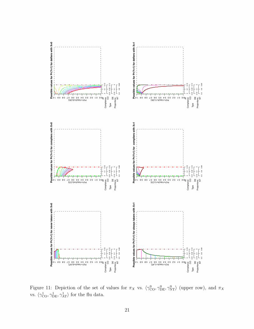
The set of values for πX vs. 〈γ0CO, γ0

DE, γ0NT〉 (upper row), and πX vs. 〈γ1

CO, γ1DE, γ1

AT〉

corresponding to the empirical distribution for p(x, y | z) are shown in Figure 11. The

empirical distribution is not consistent with there being no Defiers (though the scales in

Figure 11 show 0 as one endpoint for the proportion πDE this is merely a consequence of the

significant digits displayed; in fact the true lower bound on this proportion is 0.0005).

We emphasize that this analysis merely derives the logical consequences of the empirical

distribution under the IV model and ignores sampling variability.

5 Bounding Average Causal Effects

We may use the results above to obtain bounds on average causal effects, for different com-

plier strata:

ACEtX(πX , γ0

tX, γ1

tX) ≡ γ1

tX(πX) − γ0

tX(πX),

lACEtX(πX) ≡ minγ0

tX

,γ1

tX

ACEtX(πX , γ0

tX, γ1

tX),

uACEtX(πX) ≡ maxγ0

tX

,γ1

tX

ACEtX(πX , γ0

tX, γ1

tX),

as a function of a feasible distribution πX ; see Table 5. As shown in the table, the values

of γ0NT and γ1

AT which maximize (minimize) ACECO and ACEDE are those which minimize

20

Pr[Y=1|do(X=0),NT]

Poss

ible

val

ues

for P

r(Y=

1) fo

r nev

er ta

kers

with

X=0

0.00.10.20.30.40.50.60.70.80.91.0

00.

10.

19AT

0.31

0.22

0.12

CO

0.19

0.1

0D

E

0.5

0.6

0.69

NT

Com

plia

nce

Type

Prop

ortio

ns:

Pr[Y=1|do(X=0),CO]Poss

ible

val

ues

for P

r(Y=

1) fo

r com

plie

rs w

ith X

=0

0.00.10.20.30.40.50.60.70.80.91.0

00.

10.

19AT

0.31

0.22

0.12

CO

0.19

0.1

0D

E

0.5

0.6

0.69

NT

Com

plia

nce

Type

Prop

ortio

ns:

Pr[Y=1|do(X=0),DE]Poss

ible

val

ues

for P

r(Y=

1) fo

r def

iers

with

X=0

0.00.10.20.30.40.50.60.70.80.91.0

00.

10.

19AT

0.31

0.22

0.12

CO

0.19

0.1

0D

E

0.5

0.6

0.69

NT

Com

plia

nce

Type

Prop

ortio

ns:

Pr[Y=1|do(X=1),AT]

Poss

ible

val

ues

for P

r(Y=

1) fo

r alw

ays

take

rs w

ith X

=1

0.00.10.20.30.40.50.60.70.80.91.0

00.

10.

19AT

0.31

0.22

0.12

CO

0.19

0.1

0D

E

0.5

0.6

0.69

NT

Com

plia

nce

Type

Prop

ortio

ns:

Pr[Y=1|do(X=1),CO]Poss

ible

val

ues

for P

r(Y=

1) fo

r co

mpl

iers

with

X=1

0.00.10.20.30.40.50.60.70.80.91.0

00.

10.

19AT

0.31

0.22

0.12

CO

0.19

0.1

0D

E

0.5

0.6

0.69

NT

Com

plia

nce

Type

Prop

ortio

ns:

Pr[Y=1|do(X=1),DE]Poss

ible

val

ues

for P

r(Y=

1) fo

r def

iers

with

X=1

0.00.10.20.30.40.50.60.70.80.91.0

00.

10.

19AT

0.31

0.22

0.12

CO

0.19

0.1

0D

E

0.5

0.6

0.69

NT

Com

plia

nce

Type

Prop

ortio

ns:

Figure 11: Depiction of the set of values for πX vs. 〈γ0CO, γ0

DE, γ0NT〉 (upper row), and πX

vs. 〈γ1CO, γ1

DE, γ1AT〉 for the flu data.

21

Group ACE Lower Bound ACE Upper Bound

NT 0 − uγ0NT(πX) 1 − lγ0

NT(πX)

CO lγ1CO(πX) − uγ0

CO(πX) uγ1CO(πX) − lγ0

CO(πX)

= γ1CO(πX , uγ1

AT(πX)) = γ1CO(πX , lγ1

AT(πX))

−γ0CO(πX , lγ0

NT(πX)) −γ0CO(πX , uγ0

NT(πX))

DE lγ1DE(πX) − uγ0

DE(πX) uγ1DE(πX) − lγ0

DE(πX)

= γ1DE(πX , uγ1

AT(πX)) = γ1DE(πX , lγ1

AT(πX))

−γ0DE(πX , lγ0

NT(πX)) −γ0DE(πX , uγ0

NT(πX))

AT lγ1AT(πX) − 1 uγ1

AT(πX) − 0

global py1,x1|z1− py1,x0|z0

py1,x1|z1− py1,x0|z0

+ πDE · lACEDE(πX) − πAT + πDE · uACEDE(πX) + πNT

= py1,x1|z0− py1,x0|z1

= py1,x1|z0− py1,x0|z1

+ πCO · lACECO(πX) − πAT + πCO · uACECO(πX) + πNT

Table 4: Upper and Lower bounds on average causal effects for different groups, as a function

of a feasible πX . Here πcNT ≡ 1 − πNT

(maximize) ACENT and ACEAT; this is an immediate consequence of the negative coefficients

for γ0NT and γ1

AT in the bounds for γxCO and γx

DE in Table 2.

ACE bounds for the four compliance types are shown for the flu data in Figure 12. The

ACE bounds for Compliers indicate that, under the observed distribution, the possibility of

a zero ACE for Compliers is consistent with all feasible distributions over compliance types,

except those for which the proportion of Defiers in the population is small.

Following [Pearl 2000; Robins 1989; Manski 1990; Robins and Rotnitzky 2004] we also

consider the average causal effect on the entire population:

ACEglobal(πX , {γxtX}) ≡

∑

tX∈DX

(γ1tX

(πX) − γ0tX

(πX))πtX;

upper and lower bounds taken over {γxtX} are defined similarly. The bounds given for ACEtX

in Table 5 are an immediate consequence of equations (8)–(11) which relate p(y | x, z) to πX

and {γxtX}. Before deriving the ACE bounds we need the following observation:

22

Possible values for ACE for always takers

P(Y=

1|do

(X=1

),AT)

− P

(Y=1

|do(

X=0)

,AT)

−1.0

−0.7

−0.4

−0.1

0.2

0.5

0.8

0 0.1 0.19AT

0.31 0.22 0.12CO

0.19 0.1 0DE

0.5 0.6 0.69NT

Possible values for ACE for compliers

P(Y=

1|do

(X=1

),CO

) − P

(Y=1

|do(

X=0)

,CO

)

−1.0

−0.7

−0.4

−0.1

0.2

0.5

0.8

0 0.1 0.19AT

0.31 0.22 0.12CO

0.19 0.1 0DE

0.5 0.6 0.69NT

ComplianceType

Proportions:

Possible values for ACE for defiers

P(Y=

1|do

(X=1

),DE)

− P

(Y=1

|do(

X=0)

,DE)

−1.0

−0.7

−0.4

−0.1

0.2

0.5

0.8

0 0.1 0.19AT

0.31 0.22 0.12CO

0.19 0.1 0DE

0.5 0.6 0.69NT

Possible values for ACE for never takers

P(Y=

1|do

(X=1

),NT)

− P

(Y=1

|do(

X=0)

,NT)

−1.0

−0.7

−0.4

−0.1

0.2

0.5

0.8

0 0.1 0.19AT

0.31 0.22 0.12CO

0.19 0.1 0DE

0.5 0.6 0.69NT

ComplianceType

Proportions:

Figure 12: Depiction of the set of values for πX vs. ACEtX(πX) for tX ∈ DX for the flu data.

Lemma 5 For a given feasible πX and p(y, x | z),

ACEglobal(πX , {γxtX})

= py1,x1|z1− py1,x0|z0

+ πDE(γ1DE − γ0

DE) + πNTγ1NT − πATγ0

AT (21)

= py1,x1|z0− py1,x0|z1

+ πCO(γ1CO − γ0

CO) + πNTγ1NT − πATγ0

AT. (22)

Proof: (21) follows from the definition of ACEglobal and the observation that py1,x1|z1=

πCOγ1CO + πATγ1

AT and py1,x0|z0= πCOγ0

CO + πNTγ0NT. The proof of (22) is similar. !

Proposition 6 For a given feasible πX and p(y, x | z), the compatible distribution which

minimizes [maximizes] ACEglobal has

〈γ0NT, γ1

AT〉 = 〈lγ0NT, uγ1

AT〉 [〈uγ0NT, lγ1

AT〉]

〈γ1NT, γ0

AT〉 = 〈0, 1〉 [〈1, 0〉]

thus also minimizes [maximizes] ACECO and ACEDE, and conversely maximizes [minimizes]

ACEAT and ACENT.

Proof: The claims follow from equations (21) and (22), together with the fact that γ0AT and

γ1NT are unconstrained, so ACEglobal is minimized by taking γ0

AT = 1 and γ1NT = 0, and

maximized by taking γ0AT = 0 and γ1

NT = 1. !

23

Possible values for ACE for population

P(Y=

1|do

(X=1

)) −

P(Y=

1| d

o(X=

0))

−1.0

−0.8

−0.6

−0.4

−0.2

0.0

0.2

0.4

0.6

0.8

1.0

0 0.1 0.19AT

0.31 0.22 0.12CO

0.19 0.1 0DE

0.5 0.6 0.69NT

Figure 13: Depiction of the set of values for πX vs. the global ACE for the flu data. The

horizontal lines represent the overall bounds on the global ACE due to Pearl.

It is of interest here that although the definition of ACEglobal treats the four compliance

types symmetrically, the compatible distribution which minimizes [maximizes] this quantity

(for a given πX) does not: it always corresponds to the scenario in which the treatment has

the smallest [greatest] effect on Compliers and Defiers.

The bounds on the global ACE for the flu vaccine data of [Hirano, Imbens, Rubin, and

Zhou 2000] are shown are shown in Figure 13.

Finally we note that it would be simple to develop similar bounds for other measures

such as the Causal Relative Risk and Causal Odds Ratio.

6 Instrumental inequalities

The expressions involved in the upper bound on πAT in (16) appear similar to those which

occur in Pearl’s instrumental inequalities. Here we show that the requirement that PX *= ∅,

or equivalently, lπAT ≤ uπAT is in fact equivalent to the instrumental inequality. This

also provides an interpretation as to what may be inferred from the violation of a specific

inequality.

Theorem 7 The following conditions place equivalent restrictions on p(x | z) and p(y | x=

0, z):

(a1) max {0, p(x = 1 | z = 0) + p(x = 1 | z = 1) − 1} ≤

24

min{

1 −∑

j p(y=j, x=0 | z=j), 1 −∑

k p(y=k, x=0 | z=1−k)}

;

(a2) max{

∑

j p(y=j, x=0 | z=j),∑

k p(y=k, x=0 | z=1 − k)}

≤ 1.

Similarly, the following place equivalent restrictions on p(x | z) and p(y | x=1, z):

(b1) max {0, p(x = 1 | z = 0) + p(x = 1 | z = 1) − 1} ≤

min{

∑

j p(y=j, x=1 | z=j),∑

k p(y=k, x=1 | z=1−k)}

;

(b2) max{

∑

j p(y=j, x=1 | z=j),∑

k p(y=k, x=1 | z=1 − k)}

≤ 1.

Thus the instrumental inequality (a2) corresponds to the requirement that the upper

bounds on p(AT) resulting from p(x | z) and p(y = 1 | x = 0, z) be greater than the lower

bound on p(AT) (derived solely from p(x | z)). Similarly for (b2) and the upper bounds on

p(AT) resulting from p(y=1 | x=1, z).

Proof: [(a1) ⇔ (a2)] We first note that:

1 −∑

jp(y=j, x=0 | z=j) ≥(

∑

jp(x=1 | z=j))

− 1

⇔∑

j (1 − p(y=j, x=0 | z=j)) ≥∑

j p(x=1 | z=j)

⇔∑

j (p(y=1 − j, x=0 | z=j) + p(x=1 | z=j)) ≥∑

j p(x=1 | z=j)

⇔∑

j p(y=j, x=0 | z=j) ≥ 0.

which always holds. By a symmetric argument we can show that it always holds that:

1 −∑

j p(y=j, x=0 | z=1 − j) ≥(

∑

j p(x=1 | z=j))

− 1.

Thus if (a1) does not hold then max{0, p(x=1 | z=0) + p(x=1 | z=1)− 1} = 0. It is then

simple to see that (a1) does not hold iff (a2) does not hold.

[(b1) ⇔ (b2)] It is clear that neither of the sums on the RHS of (b1) are negative,

hence if (b1) does not hold then max{0, p(x = 1 | z = 0) + p(x = 1 | z = 1) − 1} =(

∑

j p(x=1 | z=j))

− 1. Now

∑

j p(y=j, x=1 | z=j) <(

∑

j p(x=1 | z=j))

− 1

⇔ 1 <∑

j p(y=j, x=1 | z=1 − j).

Likewise

∑

j p(y=j, x=1 | z=1 − j) <(

∑

j p(x=1 | z=j))

− 1

⇔ 1 <∑

j p(y=j, x=1 | z=j).

25

Thus (b1) fails if and only if (b2) fails. !

This equivalence should not be seen as surprising since [Bonet 2001] states that the

instrument inequalities (a2) and (b2) are sufficient for a distribution to be compatible with

the binary IV model. This is not the case if, for example, X takes more than 2 states.

6.1 Which alternatives does a test of the instrument inequalities

have power against?

[Pearl 2000] proposed testing the instrument inequalities (a2) and (b2) as a means of testing

the IV model; [Ramsahai 2008] develops tests and analyzes their properties. It is then natural

to ask what should be inferred from the failure of a specific instrumental inequality. It is, of

course, always possible that randomization has failed. If randomization is not in doubt, then

the exclusion restriction (1) must have failed in some way. The next result implies that tests

of the inequalities (a2) and (b2) have power, respectively, against failures of the exclusion

restriction for Never Takers (with X = 0) and Always Takers (with X = 1):

Theorem 8 The conditions (RX), (RYX=0) and (EX=0) described below imply (a2); simi-

larly (RX), (RYX=1) and (EX=1) imply (b2).

(RX) Z ⊥⊥ tX equivalently Z ⊥⊥Xz=0, Xz=1 :

(RYX=0) Z ⊥⊥ Yx=0,z=0 | tX = NT; Z ⊥⊥ Yx=0,z=1 | tX = NT;

(RYX=1) Z ⊥⊥ Yx=1,z=1 | tX = AT; Z ⊥⊥ Yx=1,z=1 | tX = AT;

(EX=0) p(Yx=0,z=0 = Yx=0,z=1 | tX = NT) = 1;

(EX=1) p(Yx=1,z=0 = Yx=1,z=1 | tX = AT) = 1.

Conditions (RX) and (RYX=x) correspond to the assumption of randomization with re-

spect to compliance type and response type. For the purposes of technical clarity we have

stated condition (RYX=x) in the weakest form possible. However, we know of no subject

matter knowledge which would lead one to believe that (RX) and (RYX=x) held, without

also implying the stronger assumption (2). In contrast, the exclusion restrictions (EX=x) are

significantly weaker than (1), e.g. one could conceive of situations where assignment had an

effect on the outcome for Always Takers, but not for Compliers. It should be noted that tests

of the instrument inequalities have no power to detect failures of the exclusion restriction

for Compliers or defier.

We first prove the following Lemma, which also provides another characterization of the

instrument inequalities:

26

Lemma 9 Suppose (RX) holds and Y ⊥⊥Z | tX = NT then (a2) holds. Similarly, if (RX)

holds and Y ⊥⊥Z | tX = AT then (b2) holds.

Note that the conditions in the antecedent make no assumption regarding the existence of

counterfactuals for Y .

Proof: We prove the result for Never Takers; the other proof is similar. By hypothesis we

have:

p(Y = 1 | Z = 0, tX = NT) = p(Y = 1 | Z = 1, tX = NT) ≡ γ0NT. (23)

In addition,

p(Y = 1 | Z = 0, X = 0)

= p(Y = 1 | Z = 0, X = 0, Xz=0 = 0)

= p(Y = 1 | Z = 0, Xz=0 = 0)

= p(Y = 1 | Z = 0, tX = CO) p(tX = CO | Z = 0, Xz=0 = 0)

+ p(Y = 1 | Z = 0, tX = NT) p(tX = NT | Z = 0, Xz=0 = 0)

= p(Y = 1 | Z = 0, tX = CO) p(tX = CO | Xz=0 = 0)(24)

+ γ0NT p(tX = NT | Xz=0 = 0).

The first three equalities here follow from consistency, the definition of the compliance types

and the law of total probability. The final equality uses (RX). Similarly, it may be shown

that

p(Y = 1 | Z = 1, X = 0)

= p(Y = 1 | Z = 1, tX = DE)p(tX = DE | Xz=1 = 0)(25)

+ γ0NT p(tX = NT | Xz=1 = 0).

Equations (24) and (25) specify two averages of three quantities, thus taking u = p(Y =

1 | Z = 0, tX = CO), v = p(Y = 1 | Z = 1, tX = DE) and w = γ0NT, we may apply the

analysis of §2.3. This then leads to the upper bound on πAT given by equation (15). (Note

that the lower bounds on πAT are derived from p(x | z) and hence are unaffected by dropping

the exclusion restriction.) The requirement that there exist some feasible distribution πX

then implies equation (a2) which is shown in Theorem 7 to be equivalent to (b2) as required.

!

27

tX , tY

Z X Y

Figure 14: Graphical representation of the model given by the randomization assumption

(2) alone. It is no longer assumed that Z does not have a direct effect on Y .

Proof of Theorem 8: We establish that (RX), (RYX=0), (EX=0) ⇒ (a2). The proof of the

other implication is similar. By Lemma 9 it is sufficient to establish that Y ⊥⊥Z | tX = NT.

p(Y = 1 | Z = 0, tX = NT)

= p(Y = 1 | Z = 0, X = 0, tX = NT) definition of NT;

= p(Yx=0,z=0 = 1 | Z = 0, X = 0, tX = NT) consistency;

= p(Yx=0,z=0 = 1 | Z = 0, tX = NT) definition of NT;

= p(Yx=0,z=0 = 1 | tX = NT) by (RYX=0);

= p(Yx=0,z=1 = 1 | tX = NT) by (EX=0);

= p(Yx=0,z=1 = 1 | Z = 1, tX = NT) by (RYX=0);

= p(Y = 1 | Z = 1, tX = NT) consistency, NT.!

A similar result is given in [Cai, Kuroki, Pearl, and Tian 2008], who consider the Average

Controlled Direct Effect, given by:

ACDE(x) ≡ p(Yx,z=1=1) − p(Yx,z=0=1),

under the model given solely by the equation (2), which corresponds to the graph in Figure

14. Cai et al. prove that under this model the following bounds obtain:

ACDE(x) ≥ p(y=0, x | z=0) + p(y=1, x | z=1) − 1, (26)

ACDE(x) ≤ 1 − p(y=0, x | z=1) − p(y=1, x | z=0). (27)

It is simple to see that ACDE(x) will be bounded away from 0 for some x iff one of the

instrumental inequalities is violated. This is as we would expect: the IV model of Figure

1 is a sub-model of Figure 14, but if ACDE(x) is bounded away from 0 then the Z → Y

edge is present, and hence the exclusion restriction (1) is incompatible with the observed

distribution.

28

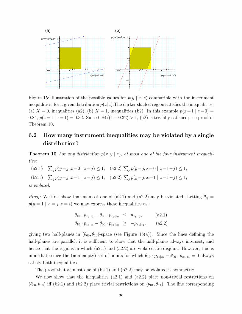
Figure 15: Illustration of the possible values for p(y | x, z) compatible with the instrument

inequalities, for a given distribution p(x|z).The darker shaded region satisfies the inequalities:

(a) X = 0, inequalities (a2); (b) X = 1, inequalities (b2). In this example p(x=1 | z=0) =

0.84, p(x=1 | z=1) = 0.32. Since 0.84/(1− 0.32) > 1, (a2) is trivially satisfied; see proof of

Theorem 10.

6.2 How many instrument inequalities may be violated by a single

distribution?

Theorem 10 For any distribution p(x, y | z), at most one of the four instrument inequali-

ties:

(a2.1)∑

j p(y=j, x=0 | z=j) ≤ 1; (a2.2)∑

j p(y=j, x=0 | z=1−j) ≤ 1;

(b2.1)∑

j p(y=j, x=1 | z=j) ≤ 1; (b2.2)∑

j p(y=j, x=1 | z=1−j) ≤ 1;

is violated.

Proof: We first show that at most one of (a2.1) and (a2.2) may be violated. Letting θij =

p(y = 1 | x = j, z = i) we may express these inequalities as:

θ10 · px0|z1− θ00 · px0|z0

≤ px1|z0, (a2.1)

θ10 · px0|z1− θ00 · px0|z0

≥ −px1|z1, (a2.2)

giving two half-planes in (θ00, θ10)-space (see Figure 15(a)). Since the lines defining the

half-planes are parallel, it is sufficient to show that the half-planes always intersect, and

hence that the regions in which (a2.1) and (a2.2) are violated are disjoint. However, this is

immediate since the (non-empty) set of points for which θ10 · px0|z1− θ00 · px0|z0

= 0 always

satisfy both inequalities.

The proof that at most one of (b2.1) and (b2.2) may be violated is symmetric.

We now show that the inequalities (a2.1) and (a2.2) place non-trivial restrictions on

(θ00, θ10) iff (b2.1) and (b2.2) place trivial restrictions on (θ01, θ11). The line corresponding

29

to (a2.1) passes through (θ00, θ10) = (−px1|z0/px0|z0

, 0) and (0, px1|z0/px0|z1

); since the slope of

the line is non-negative, it has non-empty intersection with [0, 1]2 iff px1|z0/px0|z1

≤ 1. Thus

there are values of (θ01, θ11) ∈ [0, 1]2 which fail to satisfy (a2.1) iff px1|z0/px0|z1

< 1. By a

similar argument it may be shown that (a2.2) is non-trivial iff px1|z1/px0|z0

< 1, which is

equivalent to px1|z0/px0|z1

< 1.

The proof is completed by showing that (b2.1) and (b2.2) are non-trivial if and only if

px1|z0/px0|z1

> 1. !

Corollary 11 Every distribution p(x, y | z) is consistent with randomization (RX) and (2),

and at least one of the exclusion restrictions EX=0 or EX=1.

6.2.1 Flu Data Revisited

For the data in Table 3, all of the instrument inequalities hold. Consequently there is no

evidence of a direct effect of Z on Y . (Again we emphasize that unlike [Hirano, Imbens,

Rubin, and Zhou 2000], we are not using any information on baseline covariates in the

analysis.) Finally we note that, since all of the instrumental inequalities hold, maximum

likelihood estimates for the distribution p(x, y | z) under the IV model are given by the

empirical distribution. However, if one of the IV inequalities were to be violated then the

MLE would not be equal to the empirical distribution, since the latter would not be a law

within the IV model. In such a circumstance a fitting procedure would be required; see

[Ramsahai 2008, Ch. 5].

7 Conclusion

We have built upon and extended the work of Pearl, displaying how the range of possible

distributions over types compatible with a given observed distribution may be characterized

and displayed geometrically. Pearl’s bounds on the global ACE are sometimes objected to

on the grounds that they are too extreme, since for example, the upper bound presupposes a

100% success rate among Never Takers if they were somehow to receive treatment, likewise

a 100% failure rate among Always Takers were they not to receive treatment. Our analysis

provides a framework for performing a sensitivity analysis. Lastly, our analysis relates the

IV inequalities to the bounds on direct effects.

Acknowledgements

This research was supported by the U.S. National Science Foundation (CRI 0855230) and

U.S. National Institutes of Health (R01 AI032475) and Jesus College, Oxford where Thomas

30

Richardson was a Visiting Senior Research Fellow in 2008. The authors used Avitzur’s

Graphing Calculator software (www.pacifict.com) to construct two and three dimensional

plots. We thank McDonald, Hiu and Tierney for giving us permission to use their flu vaccine

data.

References

Balke, A. and J. Pearl (1997). Bounds on treatment effects from studies with imperfect

compliance. Journal of the American Statistical Association 92, 1171–1176.

Bonet, B. (2001). Instrumentality tests revisited. In Proceedings of the 17th Conference on

Uncertainty in Artificial Intelligence, pp. 48–55.

Cai, Z., M. Kuroki, J. Pearl, and J. Tian (2008). Bounds on direct effects in the presence

of confounded intermediate variables. Biometrics 64, 695–701.

Chickering, D. and J. Pearl (1996). A clinician’s tool for analyzing non-compliance. In

AAAI-96 Proceedings, pp. 1269–1276.

Erosheva, E. A. (2005). Comparing latent structures of the Grade of Membership, Rasch,

and latent class models. Psychometrika 70, 619–628.

Fienberg, S. E. and J. P. Gilbert (1970). The geometry of a two by two contingency table.

Journal of the American Statistical Association 65, 694–701.

Hirano, K., G. W. Imbens, D. B. Rubin, and X.-H. Zhou (2000). Assessing the effect of

an influenza vaccine in an encouragement design. Biostatistics 1 (1), 69–88.

Manski, C. (1990). Non-parametric bounds on treatment effects. American Economic Re-

view 80, 351–374.

McDonald, C., S. Hiu, and W. Tierney (1992). Effects of computer reminders for influenza

vaccination on morbidity during influenza epidemics. MD Computing 9, 304–312.

Pearl, J. (2000). Causality. Cambridge, UK: Cambridge University Press.

Ramsahai, R. (2008). Causal Inference with Instruments and Other Supplementary Vari-

ables. Ph. D. thesis, University of Oxford, Oxford, UK.

Robins, J. (1989). The analysis of randomized and non-randomized AIDS treatment tri-

als using a new approach to causal inference in longitudinal studies. In L. Sechrest,

H. Freeman, and A. Mulley (Eds.), Health Service Research Methodology: A focus on

AIDS. Washington, D.C.: U.S. Public Health Service.

31

Robins, J. and A. Rotnitzky (2004). Estimation of treatment effects in randomised tri-

als with non-compliance and a dichotomous outcome using structural mean models.

Biometrika 91 (4), 763–783.

32