analysis of wind energy potential in selected regions...

ANALYSIS OF WIND ENERGY POTENTIAL IN

SELECTED REGIONS IN NIGERIA AS A POWER

GENERATION SOURCE

A THESIS SUBMITTED TO THE GRADUATE

SCHOOL OF APPLIED SCIENCES

OF

NEAR EAST UNIVERSITY

By

GODSTIME ERHABOR

In Partial Fulfillment of the Requirements for

the Degree of Master of Science

in

Mechanical Engineering

NICOSIA, 2019

Godstime ERHABOR: ANALYSIS OF WIND ENERGY POTENTIAL IN

SELECTED REGIONS IN NIGERIA AS A POWER GENERATION SOURCE

Approval of Director of Graduate School of

Applied Sciences

Prof. Dr. Nadire ÇAVUŞ

We certify this thesis is satisfactory for the award of the degree of Master of Science in

Mechanical Engineering

Examining Committee in Charge:

Assist. Prof. Dr. Youssef KASSEM Supervisor, Department of Mechanical

Engineering, NEU

Prof. Dr. Adil AMIRJANOV Department of Mechanical Engineering,

NEU

Assoc. Prof. Dr. Hüseyin ÇAMUR Department of Mechanical Engineering,

NEU

I hereby declare that, all the information in this document has been obtained and presented

in accordance with academic rules and ethical conduct. I also declare that, as required by

these rules and conduct, I have fully cited and referenced all material and results that are not

original to this work.

Name, Last Name:

Signature:

Date:

ii

ACKNOWLEDGEMENTS

From the beginning of my journey in Near East University until this day, Assist. Dr. Youssef

KASSEM, the godfather of Mechanical Engineering Department’s students, and Assoc.Prof.

Dr. Hüseyin ÇAMUR, my mentor and my very first advisor, were the most helpful and

supportive people I met in the department. Their endless encouragement and advises was the

main cause of this study completion, they believed in me since day one, for all these, words

are powerless to express my gratitude to both of you, Thank you so much.

To my beloved family especially my parents who were always keen to listen to my challenges

and supported me in all ways to the best of their ability, I am so thankful for your support, I

would have never reach to this point without you, and I greatly appreciate you all.

iii

To my parents, with love…

iv

ABSTRACT

This study shows the wind speed characteristics and wind power potential of four locations in

Nigeria: Edo, Delta, Abia and Bauchi from 2008- 2017 duration. The data was obtained from

the Nigerian Meteorological Center Furthermore, to examine the capabilities of a vertical axis

wind turbine to generate power at the locations.

The annual mean wind speed for the four locations in this study is ranges from 2.3 knots to 4.7

knots which is 1.2 m/s to 2.4 m/s respectively at a 10m; this indicates the locations have low

wind energy potential. The GEV proved to be the best fit to the wind speed data for the

locations of Delta, Abia, and Bauchi, while Weibull analysis for Edo. It was observed that Edo

has the highest winds and its wind power analysis is the best location for collecting wind

energy.

The annual wind power values ranged from 2.30W/m2 to 9.34W/m2 at 10m height. These

values shows that the wind power potential of these locations could be possible to exploited

using small-scale wind turbines at the locations. It was concluded that VAWT with a

comparable rated output would produce more power in the locations than a HAWT due to less

noise and more efficient. Subsequently, with a power rating of 4kW the Wind-dam had the

lowest energy production cost among the considered vertical axis wind turbine.

Keywords: Economic analysis; Nigeria; Distribution functions; Statistical analysis; Vertical

axis wind turbine; Wind speed characteristics

v

ÖZET

Bu çalışma, 2008 - 2017 süresinden itibaren Edo, Delta, abia ve Bauchi olmak üzere

nijerya'daki dört yerin rüzgar hızı özelliklerini ve rüzgar enerjisi potansiyelini göstermektedir.

Veriler Nijeryalı Meteoroloji Merkezi'nden elde edildi ayrıca, yerlerde güç üretmek için dikey

eksenli rüzgar türbininin yeteneklerini incelemek. Bu çalışmada dört lokasyon için yıllık

ortalama rüzgar hızı, 2.3 knot ile 4.7 knot arasında değişmektedir; bu, 10m'de sırasıyla 1.2 m/s

ila 2.4 m / s arasındadır; bu, konumların düşük rüzgar enerjisi potansiyeline sahip olduğunu

gösterir. Gev, Edo için Weibull analizi yaparken, Delta, Abia ve Bauchi'nin yerleri için rüzgar

hızı verilerine en uygun olduğunu kanıtladı .Edo'nun en yüksek rüzgara sahip olduğu ve rüzgar

enerjisi analizinin rüzgar enerjisini toplamak için en iyi yer olduğu gözlenmiştir. Yıllık rüzgar

enerjisi değerleri 2.30 W/m2 ila 9.34 W/m2 arasında 10m yükseklikte değişiyordu. Bu

değerler, bu konumların rüzgar enerjisi potansiyelinin, konumlarda küçük ölçekli rüzgar

türbinleri kullanılarak sömürülebileceğini göstermektedir. Karşılaştırılabilir bir nominal çıkışa

sahip VAWT'NİN, daha az gürültü ve daha verimli olması nedeniyle bir HAWT'TAN daha

fazla güç üreteceği sonucuna varılmıştır. Daha sonra, 4kw güç derecesi ile Winddam, dikey

eksenli rüzgar türbini arasında en düşük enerji üretim maliyetine sahipti.

Anahtar kelime: Ekonomik analiz; Nijerya; dağıtım fonksiyonları; istatistiksel analiz; dikey

eksenli rüzgar türbini; rüzgar hızı özellikleri

1

CHAPTER 1

INTRODUCTION

1.1 Overview

The demand for energy increases as the world population growth rises. To improve the

standard of living in developing countries and maintain the growth in industrialized countries,

energy use cannot be avoided. Renewable energy in a higher share can be used more

efficiently as an energy source. Today, the rise of wind energy use is a developing technology.

Wind energy is a local resource and it has been the most promising clean source of energy all

over the world, to combat and overcome the existing power issues it is vital to conduct a

research on the technical and economical possibilities. (Köse 2004)

The main source of energy demand is fossil fuels and it plays a key role to the world supply.

However, fossil fuels have a negative environmental impact and it is in limited resource.

Therefore, energy sources rational utilization and management, and renewable energy source

usage are vital. (Aynur.U 2010)

Environmental protection, energy security and sustainable development are achieved by an

increasing role of Renewable energy. Nowadays, other forms of renewable energy

technologies are becoming more expensive but wind energy as one of the cleanest form is

highly recommended because of its falling cost. (Ahmed O Hanane 2010)

Wind energy can be captured by blowing wind into turbines that convert kinetic energy from

wind into mechanical energy and subsequently into electrical energy. (Alam HM 2010)

Countries in Europe and Northern America use wind energy to produce electricity on a large

scale. (Ahmed SA 2010)

2

Wind power generation potential and its characteristics can be observed by carrying out a

necessary a long term meteorological observation. Wind speed data is needed to acquire such

potential. (Aynur U 2010)

1.2 Electricity Problems in Nigeria

The hindered industrialization and economic growth in Nigeria is as a result of poor

generation means. The power crisis has been reformed by various means but no visible

changes seem to be happening. The industries which were once there moved to a more secure

and environmental friendly nation with a stable power supply. Furthermore, basic amenities

such as healthcare system, water supply and petroleum distribution are in jeopardy due to

terrible state of the nation’s economy and inability to meet its electricity demand. The major

challenges researchers find in Nigeria’s power generation are factors such as obsolete

equipments, poor power plant maintenance, and vandalism of energy producing equipments

but through a well planned maintenance, producing methodology and funding it can be

revived.

1.3 Renewable Energy

Natural resources which energy can be generated from is Renewable energy. This implies

energy resources can be replenished in a short amount of time, which in turns makes it an

unlimited source of energy. Electric power is generated by using various forms of conversion

methods to convert renewable energy sources such as wind, solar and geothermal.

1.3.1 Wind power

Wind power is clean source of energy and has zero emissions. It also has a low fossil fuel

dependence.

3

Pros

1. It is a cheap form of energy

2. It requires minimum space

3. It functions at any time of day as long as wind blows

Cons

1. Centrifugal forces damages blades

2. Wind is need to generate electricity i.e. no wind no power

1.3.2 Solar energy

Solar energy converts sunlight into electricity by means of photovoltaic or concentrated

sunlight.

It has different types of collectors namely Compound Parabolic Concentrator, Flat- plate

Collector, Parabolic through Collector and Evacuated- tube Collector.

1.4 Aim of Study

In Nigeria little is known about wind potential and limited studies have been done on it. This

thesis aims to study, analyze, evaluate and justify the following research objectives for the

following states in Nigeria (Edo, Delta, Abia, Bauchi).

1. Wind speed, direction and potential at selected locations.

2. Wind speed characteristics according to time (months, seasons and years).

3. Does wind speed change with respect to height at different location?

4. Which distribution function is best to evaluate wind potential data?

5. Which Locations gives the highest capacity factors and least cost?

4

6. The most fitting wind turbine class for each location.

7. Is wind energy a good option for a given location?

1.5 Overview of Thesis

Chapter 1 gives an overview of renewable energy and its demand, also a short description on

the electricity problems in Nigeria and the aim of the study.

In chapter 2, recent studies on wind potential is discussed as well as the economic analysis of

the wind turbine and wind power density.

Chapter 3 shows the different methods used to analyze the meteorological data and the use of

simulation tools used for this study. It shows the description of the location chosen for this

study and ten models used to evaluate wind potential.

In chapter 4, the results obtained from the study as well as analysis done with the mentioned

parameters.

Chapter 5 gives the detailed report on the findings and conclusion of the study.

5

CHAPTER 2

LITERATURE REVIEW AND ECONOMIC ANALYSIS

2.1 Recent Studies on Wind Potential

In past and recent years, wind energy studies have been carried out across the world. (M.S.

Adaramola et al., 2011) investigated and analyzed the wind energy potential and economic

analysis using wind speed data with a time frame of 19 to 37 year period at a 10 meter height,

in six selected locations in North- central Nigeria. Levied cost method was used to evaluate

small and medium size turbines for the selected locations.It was concluded that energy cost

decreases, discount rate decreases by increasing the escalation rate of inflation.WECS was

used by (O.S. Ohunakin et al., 2011) to evaluate production of electricity for a 36 year period

data in 7 locations in Nigeria. A Technical assessment was conducted and the data was

subjected to a 2- parameter Weibull analysis for four commercial wind turbines. Nordex N80 -

2.5MW wind turbine was most suitable for Kano which had the highest annual wind power

and Suzlon S52 for Yelwa which had the lowest annual wind power.At 15 different locations

(T.R. Ayodele et al., 2016) evaluated the possibility of producing electricity by utilizing wind

energy. For a period of 4-16 years they used a daily average of wind speeds at 10 meter height.

The capacity factor estimation for the appropriate wind turbine was used for each location.

The unit cost of energy for the turbines was calculated by using the present value cost method.

The results showed high rates of wind speeds at Jos and Kano, also they are economically

viable for grid integration application.(Olayinka S. Ohunakin et al., 2011) investigated the

wind energy potential in Jos using a 37 year wind speed data at a height of 10m subjected to a

0- parameter Weibull Analysis. The location Jos is suitable for wind turbine application as the

analysis shows it falls under class 7 of the international system of wind classification. Two

commercial turbines AN Bonus 300kW/33 and AN Bonus 1 MW/54 were evaluated by using

the capacity factor estimates. The maintenance cost and relative estimated costs of € 0.025, €

6

0.015, € 0.016 per kWh of energy were produced under two different values of yearly

operations.

Investigating detailed knowledge of the wind characteristics, such as speed, direction,

continuity, and availability determines the wind energy potential for the selected site. Thus,

the wind power plants are obtained by selecting a proper wind turbine and micro sitting

process.In the most recent years, various countries worldwide have studied numerous research

on wind characteristics and wind power potential. In the Mamara region of Turkey, Go¨kc¸ek

et al. (2007) researched the wind characteristics and wind potential of Kırklareli province. The

data observed yielded the annual mean power density and weibull function to be 13.85W/m2

and 142.75. In the eastern Mediterranean region, hourly wind data was used to find the wind

energy potential from seven stations, from 1992-2001 by Sahin et al. (2005). The mean power

density of 500 W/m2 was found in many areas of this region at 25m from the ground.

Along the Mediterranean Sea in Egypt, Ahmed Shata and Hanitsch (2006) evaluated the wind

energy potential by using wind data from ten coastal meteorological locations. The locations

monthly and annual mean wind power densities were derived. Sidi Barrani, Mersa Matruh,

and El Dabaa proved to be the best out of all ten studied locations. At El Dabaa station a wind

turbine of capacity 1MW was found to generate an energy output per year of 2718 MWh, and

the production costs were 2V cent/kWh. In Lithuania, Marciukaitis et al. (2008) researched the

power situation and future potential of wind energy usage. It was evualted that the average

annual wind speed in Lithuania is 6.4m/s at 50m above ground. Kaldellis (2008) examined the

wind potential of the Aegean Archipelago. He showed that the Aegean Archipelago has an

excellent wind potential and wind energy applications can substantially contribute to fulfilling

the energy needs of the island.

2.2 Wind power density (WPD)

The representative value of the wind energy potential of an area is the Wind power density

(WPD). It details the distribution of wind energy via a model of wind power density at several

7

wind velocity values. The wind speed relies on the air density as well as the WPD as

illustrated by:

𝑃

𝐴=1

2𝜌𝑣3

(3.1)

𝑃

𝐴 =

1

2𝜌𝑣3𝑓(𝑣)

(3.2)

Moreover, the mean wind power density can be estimated using Eq. (3.3)

�̅�

𝐴=1

2𝜌�̅�3

(3.3)

Where A is a swept area in m2, P is the wind power in W, ρ is the air density (ρ= 1.225kg/m3)

and v is wind speed in (m/s).

2.3. Wind Speed Variation

The simple power law model is usually used to convert the wind speeds at different heights,

for wind energy assessments. It is depicted as

𝑣

𝑣10= (

𝑧

𝑧10)𝛼

(3.4)

8

Where v10 is the wind speed at the original height z10, v is the wind speed at the wind turbine

hub height z, and α is the surface roughness coefficient, it is dependent on the locations

characteristics. The wind speed data was measured at the height of 10 m above the ground;

therefore, the value of α can be obtained from the following expression

𝛼 =0.37 − 0.088𝑙𝑛(𝑣10)

1 − 0.088𝑙𝑛(𝑧10 10⁄ ) (3.5)

2.4 Analysis of Wind Performance

2.4.1 The energy output of wind turbines

Total power output (Ewt) of wind turbines can be expressed by Equation (3.7) Futhermore, the

power curve of the wind turbines can be estimated with a parabolic law, as given by

(Equation (3.6)).

𝑃𝑤𝑡(𝑖) =

{

Pr

𝑣𝑖2 − 𝑣𝑐𝑖

2

𝑣𝑟2 − 𝑣𝑐𝑖2 𝑣𝑐𝑖 ≤ 𝑣𝑖 ≤ 𝑣𝑟

1

2𝜌𝐴𝐶𝑝𝑣𝑟

2 𝑣𝑟 ≤ 𝑣𝑖 ≤ 𝑣𝑐𝑜

0 𝑣𝑖 ≤ 𝑣𝑐𝑖𝑎𝑛𝑑𝑣𝑖 ≥ 𝑣𝑐𝑜

(3.6)

𝐸𝑤𝑡 =∑𝑃𝑤𝑡(𝑖) × 𝑡

𝑛

𝑖=1

(3.7)

where vi is the vector of the possible wind speed at a given location, Pwt(i) is the vector of the

equivalent wind turbine output power in W, vci is the cut-in wind speed (m/s), Pr is the rated

9

power of the turbine in W, vco is the cut-out wind speed (m/s) of the wind turbine and vr is the

rated wind speed (m/s). Cp is the coefficient of performance of the turbine, and it is a function

of the tip speed ratio and the pitch angle. The coefficient of performance is considered to be

constant for the whole range of wind speed and can be calculated as

𝐶𝑝 = 2𝑃𝑟

𝜌𝐴𝑣𝑟3

(3.8)

2.4.2 Capacity factor (CF)

The capacity factor (CF) of a wind turbine is the fraction of the total energy generated by the

wind turbine over a period of time to its potential output if it had operated at a rated capacity

throughout the whole time period. The capacity factor of a wind turbine based on the local

wind program of a certain site could be calculated as

𝐶𝐹 = 𝐸𝑤𝑡𝑃𝑟 . 𝑡

(3.9)

2.5. Economic Analysis Of Wind Turbines

Different methods have been used to calculate the wind energy cost such as PVC methods].

The Present Value of Costs (PVC) is expressed as:

𝑃𝑉𝐶 = [𝐼 + 𝐶𝑜𝑚𝑟 (1 + 𝑖

𝑟 − 𝑖) × [1 − (

1 + 𝑖

1 + 𝑟)𝑛

] − 𝑆 (1 + 𝑖

1 + 𝑟)𝑛

] (3.10)

10

where r is the discount rate, Comr is the cost of operation and maintenance, n is the machine

life as designed by the manufacturer, i is the inflation rate,I is the investment summation of

the turbine price and other initial costs, including provisions for civil work, land,

infrastructure, installation, and grid integration and S is the scrap value of the turbine price

and civil work.

The cost per kWh of electricity produced (UCE) can be expressed by the following:

𝐸𝐺𝐶 =𝑃𝑉𝐶

𝑡 × 𝑃𝑟 × 𝐶𝐹 (3.11)

2.5.1 Wind turbines cost analysis

Cost for almost any wind turbine product could be expressed as cash per kilowatt (1dolar1

/kW).

This specific cost expression is able to differ among manufacturers. Consequently, in the

simplification on the analysis, the range of the cost for every one of the classes is given in the

table 4.3 under (Mathew, 2007).

11

Table 2.1: Cost ranges of a wind turbines (Mathew, 2007)

Power Rate (kW) Specific cost ($/kW) Average cost ($/kW)

10–20 2200–2900 2550

20–200 1500–2300 1900

>200 1000–1600 1300

The financial growth of every wind power generation plant is within direct proportionality to

its ability to generate electricity at low cost of operation (Kristensen et al., 2000). To

determine the cost of energy generation by wind turbine, the following parameters are to be

considered (Gökçek as well as Genç, 2009):

1. Turbine electrical energy generation over average wind speed.

2. Maintenance and operational expenses (Co&m).

3. Discount rate

4. Investment cost, which includes the basis as well as the power grid connection costs.

5. Plant lifetime.

The parameters detailed above are mainly location dependent.Thus, the key variables are

definitely the turbine efficiency as well as the expenditure costs.

The electrical energy production of wind turbines is subject to wind conditions; thusly, the

best alternative on the plant site is an essential component in acquiring financial reasonability

(Belabes et al., 2015).

12

For last literature, various techniques have been worn inside the calculation of blowing wind

control cost that is discussed inside (Lackner et al., 2010).

The present value cost method (PVC), will be the adopted way for the assessment, and

furthermore this is a result to consider related monetary components just as accounts for the

different occurrences of costs and incomes. The PVC method can be expressed as

𝑃𝑉𝐶 = [𝐼 + 𝐶𝑜𝑚𝑟 (1+𝑖

𝑟−𝑖) × [1 − (

1+𝑖

1+𝑟)𝑛

] − 𝑆 (1+𝑖

1+𝑟)𝑛

](3.12)

where r is the discount rate, Comr is the cost of maintenance and operation, n is the machine

life as designed by the manufacturer, i is the inflation rate,I is the investment summation on

the turbine price along with other initial expenses, including provisions for municipal labor,

installation, infrastructure, land, and then power system integration as well as S scrap

valuation on the turbine price as well as civil labor.

Table 2.2: PVC method variables values (Diaf and Notton, 2013)

Parameter Value Parameter Value

r[%] 8 I [%] 68

i[%] 6 S [%] 10

n [year] 20 & [%] 7

13

The cost per kWh of electricity generated (UCE)as expressed by Gass et al. (2013) can be

determined by the following expression

𝑈𝐶𝐸 =𝑃𝑉𝐶

𝑡×𝑃𝑟×𝐶𝐹 (3.13)

14

CHAPTER 3

METHODOLOGY

3.1 Materials and Methods

In this section, at a height of 10m at four locations in Nigeria, the statistical analysis of wind

speed is discussed. The wind power densities at the studied locations were obtained by using

ten distribution functions. The wind speed at different hub heights was estimated by using the

power law method. The yearly energy outputs, capacity factor and electricity generated cost

were analyzed for small scale wind turbines of different types and sizes. Figure 3.1 shows the

procedure analysis of this study.

Figure 3.1: The flowchart for analysis steps of the study

15

3.2 Description of Selected Locations

Table 3.1: Description of locations

Location

Bauchi Edo Delta Abia

Latitude 10.6371° N 6.5438° N 5.5325° N 5.4309° N

Longitude 10.0807° E 5.8987° E 5.8987° E 7.5247° E

Population 2.17million 3.2million 4.1million 2.3million

Period of records 2008-2017 2008-2017 2008-2017 2008-2017

Figure 3.2: The map of studied locations (Nations online project)

16

3.3 Wind Data Source

A monthly wind data for ten years (2008-2017) for the selected locations Edo, Delta, Abia and

Bauchi, where available for this study and collected collect from the Nigerian Meteorological

Agency (NiMet). The data was collected at a height of 10m on an hourly basis by using a cup

anemometer and later the monthly average was calculated. The large quantity of data collected

aims to increase accuracy of the results evaluated. This is illustrated in Table 3.1

3.4 Distribution Function and Estimated Model

It is essential that wind speed data is acquired for the assessment of renewable resources.

Various types of distribution functions provide wind speed data for selected locations (Ouarda

et al., 2015; Aries et al., 2018; Allouhi et al., 2017). In this study, ten various probability

distribution functions will be utilized for the study of wind speed distribution at the selected

locations. The ten distribution functions used in this study will show the probability

distribution function (PDF) and cumulative distribution function (CDF) of selected locations.

The parameter values of every distribution function used will make use of the Maximum

likelihood method in this study. Lastly, Matlab R2015a and Easy fit software with a CPU-

Intel Xeon E5-16XX, 64GB ram, 8 core and 64-bit Operating System were used to determine

the parameters of the distribution functions.

Weibull distribution (W)

To estimate the wind power density and wind speed, Weibull distribution is usually used in

studies (Bilal et al., 2013).The measured data is usually a good match (Akdaǧ et al., 2010).

The probability density function (PDF) of the wind speed is given by:

𝑷𝑫𝑭 = (𝒌

𝒄) (

𝒗

𝒄)𝒌−𝟏

𝒆𝒙𝒑(− (𝒗

𝒄)𝒌

) (3.1)

17

While the Cumulative Distribution Function (CDF) is given as:

𝑪𝑫𝑭 = 𝟏 − 𝒆𝒙𝒑(−(𝒗

𝒄)𝒌

) (3.2)

Where; c is the scale parameter, it is the same unit of speed (m/s), and k is the shape

parameter, which is dimensionless and v is the speed of the wind.

Gamma distribution (G)

It is a broadly used distribution function in wind evaluation studies, because it is usually

associated with exponential and normal distributions (Belabes et al., 2015).

The probability density function (PDF) of the Gamma distribution function is given by:

𝑃𝐷𝐹 =𝑣𝛽−1

𝛼𝛽𝛤(𝛽)exp (−

𝑣

𝛽) (3.3)


𝐶𝐷𝐹 =𝛾(𝛽,

𝑣

𝛼)

𝛤(𝛽) (3.4) (3.4)

Where, α is the scale parameter, and β is the shape parameter, which is dimensionless and v is

the wind speed.

18

Lognormal distribution (LN)

The Galton distribution or Lognormal as it is commonly know, is a probability distribution of

the normally distributed logarithmic variables of wind speed (Allouhi et al., 2017). The PDF

of this function can be a obtained from this equation;

𝑃𝐷𝐹 =1

𝑣𝜎√2𝜋𝑒𝑥𝑝 [−

1

2(𝑙𝑛(𝑣)−𝜇

𝜎)2

] (3.5)


𝐶𝐷𝐹 =1

2+ 𝑒𝑟𝑓 [

𝑙𝑛(𝑣)−𝜇

𝜎√2] (3.6)

Where, μis the scale parameter, and σis the shape parameter, which are dimensionless and v is

the wind speed.

Logistic (L)

The probability distribution function is given by:

𝑃𝐷𝐹 =exp(−

𝑣−𝜇

𝜎)

𝜎{1+exp(−𝑣−𝜇

𝜎)}2 (3.7)


19

𝐶𝐷𝐹 =1

1+exp(−𝑣−𝜇

𝜎) (3.8)

Where, σ is the scale parameter, and μ is the area parameter, which are dimensionless and v is

the wind speed.

Log-logistic distribution function (LL)

It is used to distribute the logistic form logarithmic variables of the wind speed (Alavi et al.,

2016). The probability distribution function is given by:

𝑃𝐷𝐹 = ((𝛽

𝛼(𝑣

𝛼)𝛽−1

)

(1 +𝑣

𝛼)𝛽⁄ )

2

(3.9)


𝐶𝐷𝐹 =1

(1+𝑣

𝛼)−𝛽 (3.10)

Where, α is the scale parameter, and β is the shape parameter, which are dimensionless and v

is the wind speed.

20

Inverse Gaussian distribution (IG)

For low speeds and low frequencies, this distribution function can be used as an alternative to

the three-parameter Weibull distribution (Bardsley, 1980). The probability distribution

function is given by:

𝑷𝑫𝑭 = (𝝀

𝟐𝝅𝒗𝟐)𝟏𝟐⁄

𝒆[−𝝀(𝒗−𝝁)𝟐

𝟐𝝁𝟐𝒗] (3.11)


𝑪𝑫𝑭 = 𝜱(√𝝀

𝒗(𝒗

𝝁− 𝟏)) + 𝒆𝒙𝒑 (

𝟐𝝀

𝝁)𝜱(−√

𝝀

𝒗(𝒗

𝝁+ 𝟏)) (3.12)

Where, μ is the mean parameter, and λ is the shape parameter, which are dimensionless and v

is the wind speed.

Generalized Extreme Value (GEV)

It is the only conceivable limit distribution of proper normalized maxima in sequence of

independent and identically distributed variables. The probability distribution function is given

by:

𝑃𝐷𝐹 =1

𝛼[1 −

𝜁(𝑣)−𝜇

𝛼]

1

𝜁−1

exp [− (1 − 1 −𝜁(𝑣)−𝜇

𝛼)

1

𝜁] (3.13)

21


𝐶𝐷𝐹 = exp [−(1 − 1 −𝜁(𝑣)−𝜇

𝛼)

1

𝜁] (3.14)

It is a three-parameter function, where, μ is the area parameter, and ζ is the scale parameter, α

is the shape parameters, which are dimensionless, and v is the wind speed.

Nakagami (Na)


𝑃𝐷𝐹 =2𝑚𝑚

𝛤(𝑚)𝛺𝑚𝑣2𝑚−1𝑒(−

𝑚

𝛺𝐺2)

(3.15)


𝐶𝐷𝐹 =𝛾(𝑚,

𝑚

𝛺𝑣2)

𝛤(𝑚) (3.16)

Where, Ω is the scale parameter, and 𝑚 is the shape parameter, which are dimensionless and v

is the wind speed.

22

Normal (N)


𝑃𝐷𝐹 =1

√2𝜋𝜎2exp (−

𝑣−𝜇

2𝜎2) (3.17)

While the Cumulative Distribution Function (CDF) is given as

𝑪𝑫𝑭 =𝟏

𝟐[𝟏 + 𝒆𝒓𝒇 (

𝒗−𝝁

𝝈√𝟐)] (3.18)

Where, σ is the standard deviation, and μ is the mean parameter, which are dimensionless and

v is the wind speed.

Rayleigh distribution

This is a continuous probability distribution function.The Rayleigh distribution commonly

occurs when wind velocity is analyzed in two dimensions. The probability distribution

function is given by:

𝑷𝑫𝑭 =𝟐𝒗

𝒄𝟐𝒆−(

𝒗

𝒄)𝟐

(3.19)


𝑪𝑫𝑭 = 𝟏 − 𝒆𝒙𝒑 [−(𝒗

𝒄)𝟐

](3.20)

23

It is a uni-parameter function where, c is the scale parameter, and v is the wind speed, which

are both measured in m/s

Table 3.2: The Statistical Distributions Expressions

Distribution function PDF CDF

Weibull (W) 𝑃𝐷𝐹 = (𝑘

𝑐) (𝑣

𝑐)𝑘−1

𝑒𝑥𝑝 (−(𝑣

𝑐)𝑘

) 𝐶𝐷𝐹 = 1 − 𝑒𝑥𝑝 (−(𝑣

𝑐)𝑘

)

Gamma (G) 𝑃𝐷𝐹 =𝑣𝛽−1

𝛼𝛽Γ(𝛽)𝑒𝑥𝑝 (−

𝑣

𝛽) 𝐶𝐷𝐹 =

𝛾 (𝛽,𝑣

𝛼)

Γ(𝛽)

Lognormal (LN) 𝑃𝐷𝐹 =1

𝑣𝜎 √2𝜋𝑒𝑥𝑝 [−

1

2(𝑙𝑛(𝑣) − 𝜇

𝜎)

2

] 𝐶𝐷𝐹 =1

2+ 𝑒𝑟𝑓 [

𝑙𝑛(𝑣) − 𝜇

𝜎 √2]

Logistic (L) 𝑃𝐷𝐹 =𝑒𝑥𝑝 (−

𝑣−𝜇

𝜎)

𝜎 {1 + 𝑒𝑥𝑝 (−𝑣−𝜇

𝜎)}2 𝐶𝐷𝐹 =

1

1 + 𝑒𝑥𝑝 (−𝑣−𝜇

𝜎)

Log-Logistic (LL) 𝑃𝐷𝐹 = ((𝛽

𝛼(𝑣

𝛼)𝛽−1

)

(1 +𝑣

𝛼)𝛽⁄ )

2

𝐶𝐷𝐹 =

1

(1 +𝑣

𝛼)−𝛽

Inverse Gaussian (IG) 𝑃𝐷𝐹 = (𝜆

2𝜋𝑣2)

12⁄

𝑒[−𝜆(𝑣−𝜇)2

2𝜇2𝑣]

𝐶𝐷𝐹 = Φ( √𝜆

𝑣(𝑣

𝜇− 1))

+ 𝑒𝑥𝑝 (2𝜆

𝜇)Φ(− √

𝜆

𝑣(𝑣

𝜇

+ 1))

Generalized Extreme

Value (GEV)

𝑃𝐷𝐹 =1

𝛼[1 −

𝜁(𝑣) − 𝜇

𝛼]

1

𝜁−1

𝑒𝑥𝑝 [−(1 − 1

−𝜁(𝑣) − 𝜇

𝛼)

1

𝜁

]

𝐶𝐷𝐹 = 𝑒𝑥𝑝 [−(1 − 1 −𝜁(𝑣) − 𝜇

𝛼)

1

𝜁

]

Nakagami (Na) 𝑃𝐷𝐹 =2𝑚𝑚

Γ(𝑚)Ωm 𝑣2𝑚−1𝑒

(−𝑚

Ω𝐺2)

𝐶𝐷𝐹 =𝛾 (𝑚,

𝑚

Ω𝑣2)

Γ(𝑚)

Normal (N) 𝑃𝐷𝐹 =1

√2𝜋𝜎2𝑒𝑥𝑝 (−

𝑣 − 𝜇

2𝜎2) 𝐶𝐷𝐹 =

1

2[1 + 𝑒𝑟𝑓 (

𝑣 − 𝜇

𝜎 √2)]

24

Rayleigh (R) 𝑃𝐷𝐹 =2𝑣

𝑐2𝑒−

(𝑣

𝑐)2

𝐶𝐷𝐹 = 1 − 𝑒𝑥𝑝 [−(𝑣

𝑐)2

]

W

k Shape parameter

LL

𝜷 Shape

parameter Na

𝒎 Shape parameter

c [m/s] Scale parameter 𝜶 Scale

Parameter 𝛀 Scale parameter

G

𝜷 Shape parameter

IG

𝝀 Shape

parameter N

𝝈 Standard deviation

𝜶 Scale Parameter 𝝁 Mean

parameter 𝝁 Mean parameter

LN

𝝈 Shape parameter

GEV

𝝁 AreaParameter R c [m/s] Scale parameter

𝝁 Scale Parameter 𝜻 Scale

Parameter

L 𝝁 Area Parameter 𝜶

Shape

Parameter

𝝈 Scale Parameter

25

CHAPTER 4

RESULTS AND DISCUSSION

4.1 Description of Wind Speed Data

The Tables 4.1 – 4.4 show the statistics for each location at a10m height. The tables represent

the mean, median, standard deviation, coefficient of variance, Skewness, Kurtosis, minimum

velocity and maximum velocity. The average wind speed varies from 2.33 knots to 4.684

knots which is about 1.2m/s to 2.4m/s respectively. The standard deviation is 0.59 in Delta and

0.82 in Edo. The Skewness values are positive in Delta and Bauchi, this shows that

distribution is right- skewed. In Edo and Abia, the Skewness values are negative making it left

– skewed. The coefficient of variance is highest in Bauchi at 34.33 and lowest in Abia at

17.41.

Table 4.1: Data collected for Edo

Locatio

n

Year Mean St Dev CoefVar Minimu

m

Median Maximum Skewness Kurtosis

Edo 2008 4.844 1.028 21.230 3.700 4.700 7.100 1.370 2.310

2009 5.578 0.976 17.490 4.100 5.300 7.200 0.320 -0.410

2010 5.344 0.805 15.060 4.200 5.600 6.500 -0.220 -1.190

2011 4.300 1.325 30.810 2.100 4.600 6.100 -0.300 -1.100

2012 6.000 0.760 12.670 5.000 5.700 7.100 0.420 -1.340

2013 6.067 0.912 15.040 4.400 6.300 7.300 -0.580 -0.020

2014 3.633 0.689 18.970 2.800 3.600 5.100 1.190 1.840

2015 3.656 0.464 12.690 3.000 3.700 4.500 0.460 -0.040

2016 3.644 0.548 15.040 2.700 3.700 4.300 -0.360 -0.700

2017 3.778 0.648 17.140 2.500 3.900 4.600 -0.980 0.660

Average 4.6844 0.8155 17.614 3.45 4.71 5.98 0.132 0.001

26

Table 4.2: Data collected for Delta

Location Year Mean St Dev CoefVar Minimum Median Maximum Skewness Kurtosis

Delta 2008 3.742 0.512 13.70 3.000 3.750 4.900 0.750 1.330

2009 3.325 0.377 11.34 2.700 3.300 3.800 -0.230 -1.040

2010 3.942 0.417 10.57 3.300 3.900 4.900 1.110 1.850

2011 4.058 0.570 14.04 3.100 4.100 5.200 0.090 0.500

2012 3.417 0.685 20.04 2.500 3.350 4.900 0.700 0.750

2013 3.392 1.108 32.67 1.500 3.250 5.300 0.020 -0.270

2014 1.883 0.395 20.98 1.200 1.900 2.400 -0.230 -1.340

2015 2.367 0.446 18.84 1.700 2.350 3.400 0.910 1.720

2016 2.050 0.723 35.27 0.900 2.150 3.300 -0.010 -0.350

2017 2.208 0.696 31.52 1.100 2.150 3.400 0.170 -0.450

Average 3.0384 0.5929 20.897 2.1 3.02 4.15 0.328 0.27

Table 4.3: Data collected for Abia

Location Year Mean StDev CoefVar Minimum Median Maximum Skewness Kurtosis

Abia 2008 4.508 0.705 15.64 3.400 4.450 6.000 0.620 0.630

2009 4.467 0.303 6.770 3.800 4.400 4.800 -0.700 0.550

2010 4.033 0.591 14.66 2.800 4.200 4.800 -0.780 0.040

2011 3.783 0.616 16.29 3.000 3.600 4.800 0.560 -1.060

2012 3.608 0.815 22.59 2.100 3.500 5.000 -0.020 -0.290

2013 3.800 0.663 17.44 2.550 3.775 5.050 -0.040 0.520

2014 3.600 0.411 11.42 2.900 3.600 4.200 -0.100 -1.120

2015 4.142 1.143 27.60 3.200 3.850 7.600 2.910 9.290

2016 4.533 0.987 21.78 3.700 4.250 7.200 1.980 4.630

2017 4.125 0.819 19.86 2.900 4.000 5.600 0.380 -0.460

Average 4.0599 0.7053 17.405 3.035 3.9625 5.505 0.481 4.0599

27

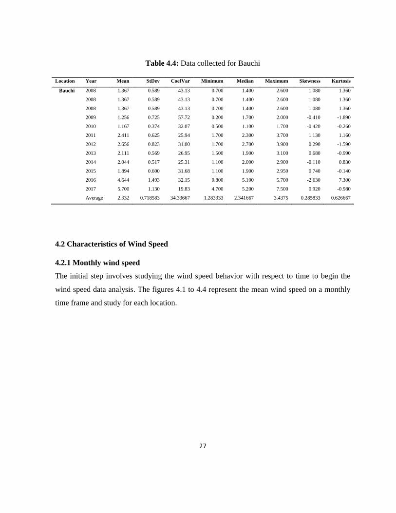
Table 4.4: Data collected for Bauchi

Location Year Mean StDev CoefVar Minimum Median Maximum Skewness Kurtosis

Bauchi 2008 1.367 0.589 43.13 0.700 1.400 2.600 1.080 1.360

2008 1.367 0.589 43.13 0.700 1.400 2.600 1.080 1.360

2008 1.367 0.589 43.13 0.700 1.400 2.600 1.080 1.360

2009 1.256 0.725 57.72 0.200 1.700 2.000 -0.410 -1.890

2010 1.167 0.374 32.07 0.500 1.100 1.700 -0.420 -0.260

2011 2.411 0.625 25.94 1.700 2.300 3.700 1.130 1.160

2012 2.656 0.823 31.00 1.700 2.700 3.900 0.290 -1.590

2013 2.111 0.569 26.95 1.500 1.900 3.100 0.680 -0.990

2014 2.044 0.517 25.31 1.100 2.000 2.900 -0.110 0.830

2015 1.894 0.600 31.68 1.100 1.900 2.950 0.740 -0.140

2016 4.644 1.493 32.15 0.800 5.100 5.700 -2.630 7.300

2017 5.700 1.130 19.83 4.700 5.200 7.500 0.920 -0.980

Average 2.332 0.718583 34.33667 1.283333 2.341667 3.4375 0.285833 0.626667

4.2 Characteristics of Wind Speed

4.2.1 Monthly wind speed

The initial step involves studying the wind speed behavior with respect to time to begin the

wind speed data analysis. The figures 4.1 to 4.4 represent the mean wind speed on a monthly

time frame and study for each location.

28

Figure 4.1: Average monthly mean wind speed in Edo

The highest mean wind speed value 5.18 knots in January and minimum of 3.87 knots in

November for Edo while the level of change recorded in speed values varies from 2.2 knots in

November 2017 and 7.3 knots March 2013.

Figure 4.2: Average monthly mean wind speed in Delta

0

1

2

3

4

5

6

JAN FEB MAR APR MAY JUN JUL AUG SEPT OCT NOV DECMo

nth

ly m

ean

win

d s

pe

ed

[kn

ots

]

EDO

0

0.5

1

1.5

2

2.5

3

3.5

4

JAN FEB MAR APR MAY JUN JUL AUG SEPT OCT NOV DEC

Mo

nth

ly m

ean

win

d s

pe

ed

[k

no

ts]

DELTA

29

The highest mean wind speed value 3.69 knots in March and minimum of 2.45 knots in

September for Delta while the level of change recorded in the speed values varies from 0.9

knots in July 2016 and 7.3 knots March 2008, February 2010 and December 2012.

Figure 4.3: Average monthly mean wind speed in Abia

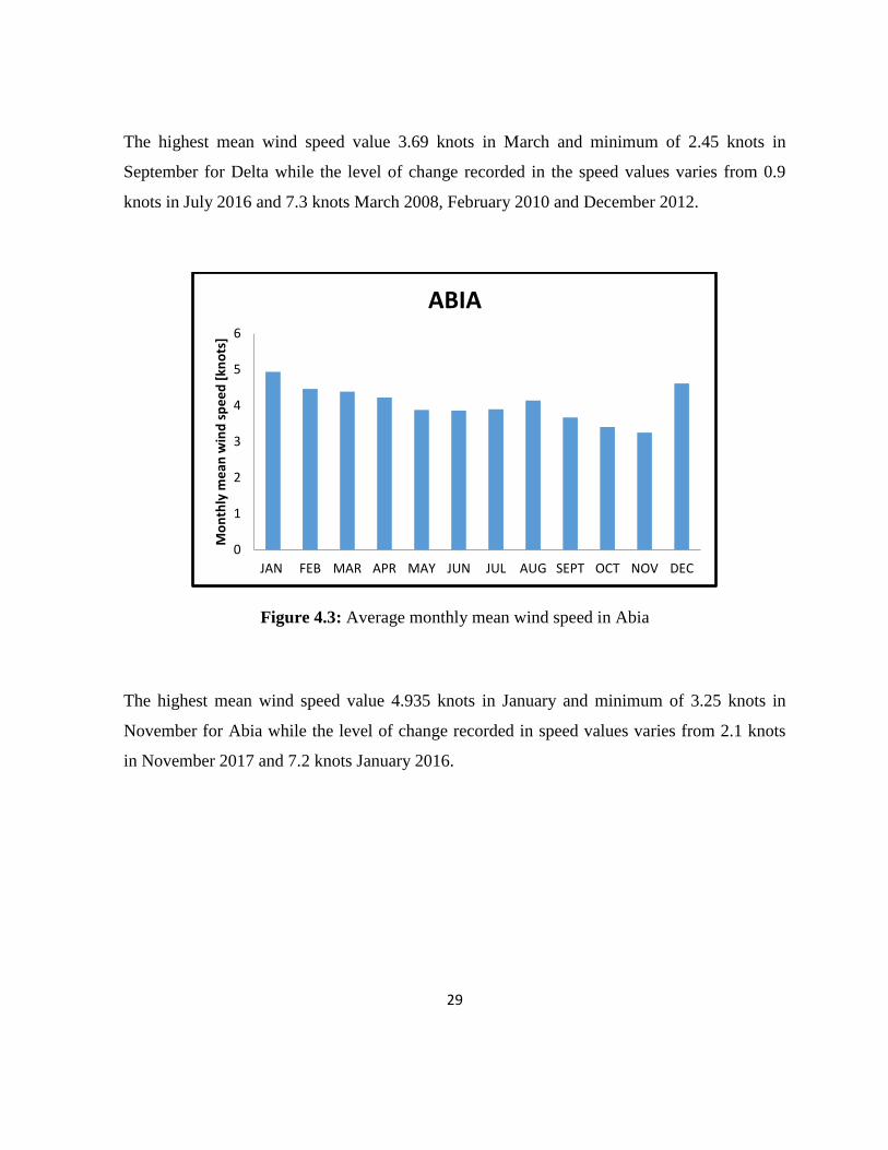
The highest mean wind speed value 4.935 knots in January and minimum of 3.25 knots in

November for Abia while the level of change recorded in speed values varies from 2.1 knots

in November 2017 and 7.2 knots January 2016.

0

1

2

3

4

5

6


Mo

nth

ly m

ean

win

d s

pe

ed

[kn

ots

]

ABIA

30

Figure 4.4: Average monthly mean wind speed in Bauchi

The highest mean wind speed value 3.235 knots in April and minimum of 1.44 knots in

January for Bauchi while the level of change recorded in speed values varies from 0.2 knots in

January 2009 and 7.5 knots February 2017.

4.2.2 Characteristics of wind speed at a 10m height

The mean wind speed data of the four locations is analyzed over time. Mean monthly wind

speed shown in Fig 4.5

0

0.5

1

1.5

2

2.5

3

3.5


Mo

nth

ly m

ean

win

d s

pe

ed

[kn

ots

]

BAUCHI

31

Figure 4.5: Annual mean wind speed at studied locations

During the ten year period in Edo, it is shown that the maximum annual mean wind speed of

5.19 knots was recorded in January, while the minimum recorded wind speed value is 3.87

knots in November. In Delta, the highest recorded value for the mean wind speed is 3.69 knots

in March, while the minimum value recorded is 2.45 knots in September. In Abia, the highest

recorded value for the mean wind speed is 4.935 knots in January, while the minimum speed

value is 3.25 in November. In Bauchi, the highest recorded value for the mean wind speed is

3.235 knots in April, while the minimum speed value recorded is 1.44 knots in January. This is

illustrated in Fig 4.6

0

0.5

1

1.5

2

2.5

3

3.5

4

4.5

5

BAUCHI EDO DELTA ABIA

Me

an w

ind

sp

ee

d [

m/s

]

32

Figure 4.6: Average monthly wind speed at four specific locations

4.3 Wind Direction

Table 4.5: Data collected for Edo

EDO

MONTHLY MEAN OF WIND DIRECTION

YEAR JAN FEB MAR APR MAY JUN JUL AUG SEPT OCT NOV DEC

2008 SE SE W SW W SW W W SW W SW SW

2009 W W W SW W SW SW W W W W SW

2010 SW W SW SW SW SW SW SW SW SW SW W

2011 SW W SW W SW W W W W SW SW W

2012 W SW W SW SW SW W SW W W W W

2013 W SW SW SW SW SW SW SW W SW W W

2014 W W SW SW W W W W W W SW W

2015 E W W W W W W SW W W W E

2016 E SW W SW W W W SW SW SW SW SW

0

1

2

3

4

5

6


BAUCHI

EDO

DELTA

ABIA

33

2017 SW SW SW SW SW SW SW SW W W SW W

Table 4.6: Data collected for Delta

DELTA

MONTHLY MEAN WIND DIRECTION

YEAR JAN FEB MAR APR MAY JUNE JULY AUG SEPT OCT NOV DEC

2008 N E S S S S S S S S S E

2009 S S S S S S S W E W N N

2010 N S S S S S S S S S S E

2011 N S S S S S S W S S N W

2012 S S S S W W W W W W W E

2013 E SW SW S S W S S S S S W

2014 E S S S S S S S S S S S

2015 E S S S S S S S S S N N

2016 N N S S S S S S S S N N

2017 N S S S S S S S SW SW S N

Table 4.7: Data collected for Abia

ABIA

MONTHLY WIND DIRECTION

YEAR JAN FEB MAR APR MAY JUN JUL AUG SEPT OCT NOV DEC

2008 NE NE SW SW SW SW SW SW SW SW SW SW

2009 SW SW SW SW SW SW SW SW SW SW SW NE


2011 NE SW SW SW SW SW SW SW SW SW SW NE

2012 NE SW SW SW SW SW SW SW SW SW SW NE

2013 NE SW SW SW SW SW SW SW SW SW SW SW

34


2015 NE SW SW SW SW SW SW SW SW SW NE NE

2016 NE NE SW SW SW SW SW SW SW SW SW NE

2017 SW NE SW SW SW SW SW SW SW SW SW NW

Table 4.8: Data collected for Bauchi

BAUCHI

MONTHLY MEAN WIND DIRECTION

YEAR JAN FEB MAR APRIL MAY JUNE JULY AUG SEPT OCT NOV DEC

2008 N N N E S S S S S E NE E

2009 E E E S S S S S S S N NE

2010 N N N N S S S S S S NE N

2011 N N E SW S S SW SW E E E NE

2012 E SW E E S S S S S SE E NE

2013 NE N E E S S S S S E NE NE

2014 NE NE E E S S S S W E E E

2015 E E E E E W W W W E E E

2016 E E E SE E W NW NW NW SE E E

2017 E E E E NW W NW NW W SE E NE

Table 4.9: Percentage occurrence of wind direction

Location Maximum Percentage Occurrence

Edo 48% W , 47.5% SW

Delta 67.5% S , 12% N , 11% W

Abia 85% SW , 14% NE

Bauchi 34% E , 28% S

35

In this study, the wind direction is taken from 16 different directions from the chosen

locations, the maximum percentage of occurrence is recorded.

As depicted Edo has 48% wind from the West and 47.5% from the South west. Delta has 67%

from the North. Abia has 85% from the South – West and 14% from the North – East. Bauchi

has 35% from the East and 28% from the South.

4.4 Parameters of Distribution Function of Wind Power Density at a10m Height

To estimate the distribution parameters and choose the best distribution functions among the

ten selected the Maximum like-hood method and Kolmogorov-Smirnov test were used for

each location. Tables 4.5-4.8 are the tabulated mean, variance and parameters of each

distribution function. Moreover, the fitted PDF and CDF models for each location were

presented in Figures 4.7-4.13.Also, Table 4.9 presents the goodness-of-fit statistics in terms of

the Kolmogorov Smirnov tests for each distribution function. The distribution function with

the lowest Kolmogorov Smirnov value will be selected to be the best model for the wind speed

distribution in the studied location. Furthermore, based on the result, Generalized Extreme

Value distribution has the lowest value, which is considered as the best distribution function to

study the wind speed distribution of all studied sites. Moreover, it is observed that the

Rayleigh distribution function cannot be used to analyze the wind potential in the studied

Location, as shown in Table 4.10.

36

Figure 4.7: Probability density function (PDF) for Abia

Figure 4.8: Cumulative distribution function (CDF) for Abia

37

Figure 4.9: Probability density function (PDF) for Bauchi

Figure 4.10: Cumulative distribution function (CDF) for Bauchi

38

Figure 4.11: Probability density function (PDF) for Delta

Figure 4.12: Cumulative distribution function (CDF) for Delta

39

Figure 4.13: Probability density function (PDF) for Edo

40

Figure 4.14: Cumulative distribution function (CDF) for Edo

Table 4.10: Annual Distribution parameters for Edo

EDO

Dis

trib

uti

on

Fu

ncti

on

s

Year 2008 2009 2010 2011 2012 2013 2014 2015 2016 2017

Actual

Mean 4.78333 5.44166 5.05 4.61666 5.76666 5.90833

3.8666

6 3.66666 3.48333

3.6833

3

G

Mean 4.78333 5.44167 5.05 4.61667 5.76667 5.90833 3.8666

7 3.66667 3.48333

3.6833

3

Variance 0.88423 0.72342 0.68620 1.86239 0.72828 0.83772 0.4832

9 0.38129 0.27679

0.7839

2

a 25.8759 40.9329 37.1646 11.4443 45.6612 41.6707 30.935

7 35.2597 43.8356

17.306

5

41

b 0.18485 0.13294 0.13588 0.40340 0.12629 0.14178 0.1249

9 0.10399 0.07946

0.2128

2

GEV

Mean 4.83649 5.43477 5.09638 4.62573 5.7677 5.91127 3.8585

7 3.66473 3.47499

3.6819

6

Variance 2.10841 0.74019 1.49695 1.70112 0.68986 0.81846 0.4514

0 0.38032 0.26278

0.7139

9

k 0.29442 0.07296 0.24315 0.67238 0.42668 0.54107 0.2576

6 0.14598 0.17775

0.3880

6

sigma 0.60804 0.73119 0.59912 1.41805 0.88211 0.98181 0.6635

9 0.56203 0.47944

0.8866

9

mu 4.239 5.06221 4.56314 4.42262 5.53229 5.70849 3.6135

3 3.41209 3.27104 3.426

IG

Mean 4.78333 5.44167 5.05 4.61667 5.76667 5.90833 3.8666

7 3.66667 3.48333

3.6833

3

Variance 0.87112 0.72600 0.69285 2.20974 0.76181 0.87344 0.4952

0 0.38772 0.27965

0.8534

6

mu 4.78333 5.44167 5.05 4.61667 5.76667 5.90833 3.8666

7 3.66667 3.48333

3.6833

3

lambda 125.636 221.95 185.88 44.5292 251.723 236.136 116.74

2 127.143 151.136

58.551

7

L

Mean 4.66513 5.37474 5.01617 4.71939 5.75684 5.95042 3.8450

2 3.62892 3.4585 3.7157

Variance 1.0017 0.81640 0.87986 1.78925 0.72846 0.93882 0.5833

7 0.40283 0.34118

0.8342

0

mu 4.66513 5.37474 5.01617 4.71939 5.75684 5.95042 3.8450

2 3.62892 3.4585 3.7157

sigma 0.55179

6

0.49815

5

0.51715

4

0.73747

4 0.47056 0.5342 0.4211

0.34992

4

0.32203

6

0.5035

55

LL

Mean 4.71326 5.41505 5.05052 4.84717 5.79909 5.99399 3.8815

6 3.66263 3.48082

3.7852

6

Variance 0.97397 0.82150 0.91882 2.76913 0.77298 1.06068 0.6245

8 0.41676 0.35101

1.0765

7

mu 1.52947 1.67559 1.60217 1.52623 1.74649 1.77646 1.3364

1 1.28316 1.23323

1.2964

2

sigma 0.11251 0.09076 0.10244 0.17714 0.08245 0.09309 0.1095

6 0.09541 0.09225

0.1447

3

LN Mean 4.78796 5.44692 5.05585 4.66056 5.77449 5.91696 3.8727 3.67132 3.48685 3.6989

42

8 6

Variance 0.95532 0.79548 0.76113 2.46696 0.83355 0.95851 0.5444

4 0.42483 0.30675

0.9452

6

mu 1.54569 1.68182 1.60587 1.48535 1.7411 1.76432 1.3361

4 1.28504 1.23654

1.2746

5

sigma 0.20205

9

0.16266

2

0.17129

4

0.32798

9

0.15713

3

0.16434

7

0.1888

3

0.17616

1

0.15785

1

0.2584

67

Table 4.10: Annual Distribution parameters for Edo cont.

Na

M e a n 4.78891 5.44331 5.05108 4.60521 5.76576 5.90724 3.86725 3.66767 3.48384 3.68131

Variance 0.914659 0.729569 0.68497 1.6637 0.707645 0.811991 0.477706 0.381546 0.276187 0.741318

m u 6.38607 10.2736 9 . 4 3 1 9 3.2979 11.8657 10.8645 7.94591 8.93377 11.1071 4.68534

o m e g a 23.8483 30.3592 26.1983 22.871 33.9517 35.7075 15.4333 13.8333 12.4133 14.2933

N

M e a n 4.78333 5.44167 5 . 0 5 4.61667 5.76667 5.90833 3.86667 3.66667 3.48333 3.68333

Variance 1.05606 0.815379 0.759091 1.6997 0.760606 0.871742 0.526061 0.424242 0.305152 0.792424

m u 4.78333 5.44167 5 . 0 5 4.61667 5.76667 5.90833 3.86667 3.66667 3.48333 3.68333

s i g m a 1.02765 0.902983 0.871258 1.30372 0.872127 0.933671 0 . 7 2 5 3 0.651339 0.552405 0.890182

R

M e a n 4.32787 4.88304 4.53609 4.23832 5.16387 5.29572 3.48157 3.29616 3 . 1 2 2 4 3.35052

Variance 5 . 1 1 7 9 6.51513 5.62221 4.9083 7.28609 7 . 6 6 2 9 3.31202 2.96866 2.66392 3.06738

B 3.45314 3 . 8 9 6 1 3.61928 3.38169 4.12017 4.22537 2.77789 2.62996 2.49132 2.67333

W

M e a n 4.76127 5.42358 5.04891 4.63398 5.76076 5.91671 3.86596 3.65283 3.48104 3.68903

Variance 1.26062 0.953185 0.788289 1.37083 0.77085 0.796306 0.534308 0.490615 0.323229 0.717232

A 5 . 1 9 5 2 5.82075 5.41133 5.0786 6.12574 6 . 2 8 8 1 4.16106 3.93496 3.71543 4.01839

B 4.84315 6.49829 6.66457 4.48962 7.77325 7.86089 6.16179 6.06864 7.21699 4.98764

43

Table 4.11: Annual Distribution parameters for Delta

DELTA

Dis

trib

uti

on

Fu

ncti

on

s

Year 2008 2009 2010 2011 2012 2013 2014 2015 2016 2017

Actual mean 3.7416 3.325 3.94166 4.05833 3.4166 3.39166 1.833 2.366 2.05 2.2083

G

Mean 3.7417 3.325 3.94167 4.05833 3.4166 3.39167 1.83 2.367 2.05 2.2083

Variance 0.2262 0.13339 0.15115 0.30203 0.4143 1.25956 0.151 0.129 0.54529 0.4732

a 60.821 82.8794 102.789 54.5309 28.171 9.13285 23.63 32.88 7.70682 10.304

b 0.0627 0.04011 0.03834 0.07442 0.1212 0.37137 0.05 0.030 0.26599 0.2143

GEV

Mean 3.7408 3.34096 3.94189 4.05891 3.4168 3.38807 1.871 2.364 2.04785 2.2039

Variance 0.2390 0.28417 0.15497 0.29793 0.4644 1.0901 0.230 0.175 0.46558 0.4240

k 0.0922 1.15733 0.03555 0.25831 0.0808 0.32896 0.855 0.629 0.33204 -0.274

sigma 0.4436 0.49324 0.32082 0.53931 0.5574 1.07024 0.471 0.358 0.70040 0.6424

mu 3.5187 3.37381 3.76764 3.85999 3.1341 3.0416 1.854 2.112 1.82242 1.9711

IG

Mean 3.7167 3.325 3.94167 4.05833 3.4667 3.39167 1.833 2.367 2.05 2.2083

Variance 0.2323 0.13622 0.14876 0.30958 0.1991 1.4814 0.112 0.136 0.65378 0.532

mu 3.74167 3.325 3.94167 4.05833 3.4167 3.39167 1.883 2.366 2.05 2.2083

lambda 225455 269.848 411.65 215.903 94.989 26.3371 41.44 76.30 13.1774 20.237

L

Mean 3.7164 3.33363 3.89431 4.06841 3.3748 3.38262 1.896 2.353 2.05701 2.1934

Variance 0.2411 0.15529 0.14459 0.30953 0.4453 1.24548 0.746 0.170 0.53347 0.500

mu 3.7164 3.33363 3.89431 4.06841 3.374 3.38262 1.896 2.353 2.05701 2.1934

sigma 0.27743 0.217263 0.209645 0.30638 0.37916 0.615288 0.255 0.2313 0.40268 0.390093

LL

Mean 3.73621 3.34603 3.90543 4.09318 3.4148 3.51953 1.9158 2.588 2.15667 2.26911

Variance 0.24585 0.16367 0.13809 0.33648 0.4614 1.81285 0.2154 0.185 0.883285 0.677822

mu 1.30943 1.20058 1.35789 1.3995 1.2053 1.19531 0.2286 0.435 0.69003 0.7618

sigma 0.07240 0.06608 0.05217 0.07720 0.1082 0.19449 0.1775 0.754 0.21677 0.1858

LN

Mean 3.74409 3.32713 3.94294 4.06226 3.4262 3.4272 1.8861 2.636 2.07692 2.224

Variance 0.25402 0.14903 0.16241 0.33885 0.4075 1.66187 0.7785 0.913 0.74163 0.5949

mu 1.3112 1.19542 1.36673 1.39158 1.2181 1.16558 0.151 0.496 0.65156 0.7429

sigma 0.13400 0.11564 0.10194 0.14256 0.147 0.36377 0.2259 0.850 0.39831 0.3368

44

Na Mean 3.74238 3.32484 3.94223 4.05827 3.4185 3.38762 1.8273 2.3682 2.04674 2.2081

Table 4.11: Annual Distribution parameters for Delta Cont.

Variance 0.235405 0.131276 0.154625 0.297927 0.417208 1.15323 0.145337 0.175803 0.49254 0.445146

mu 14.9957 21.1749 25.2503 13.9418 7.12102 2.59529 6.21484 8.09341 2.23115 2.84722

omega 14.2408 11.1858 15.6958 16.7675 12.1033 12.6292 3.69 5.78333 4.68167 5.32083

N

Mean 3.74167 3.325 3.94167 4.05833 3.41667 3.39167 1.88333 2.36667 2.05 2.20833

Variance 0.262652 0.142045 0.173561 0.32447 0.468788 1.22811 0.156061 0.198788 0.522727 0.48447

mu 3.74167 3.325 3.94167 4.05833 3.41667 3.39167 1.88333 2.36667 2.05 2.20833

sigma 0.512495 0.376889 0.416606 0.569622 0.684681 1.1082 0.395045 0.445856 0.722999 0.696039

R

Mean 3.34436 4.88304 3.51105 3.62893 3.08317 3.14943 1.70239 2.13125 1.91754 2.04425

Variance 3.05611 6.51513 3.36835 3.59834 2.5974 2.71024 0.791881 1.24111 1.00469 1.14186

B 2.66841 3.8961 2.80141 2.89547 2.46001 2.51288 1.35831 1.70049 1.52998 1.63108

W

Mean 3.71996 3.32758 3.91626 4.04543 3.40279 3.39625 1.88926 2.35293 2.05373 2.21149

Variance 0.346074 0.136459 0.260421 0.365581 0.540656 1.11156 0.136753 0.245724 0.46557 0.448319

A 3.96346 3.48551 4.13174 4.29732 3.69251 3.77037 2.03769 2.54924 2.28897 2.4514

B 7.47134 10.8874 9.18791 7.93746 5.32893 3.57556 5.93463 5.47834 3.31564 3.67614

Table 4.12: Annual Distribution parameters for Abia

ABIA

Distributi

on

Functions

Year 2008 2009 2010 2011 2012 2013 2014 2015 2016 2017

Actual

Mean

4.5083

3

4.4666

6

4.0333

3

3.7833

3

3.6083

3 3.8 3.6

4.1416

6

4.5333

3 4.125

45

G

Mean 4.5083

3

4.4666

7

4.0333

3

3.7833

3

3.6083

3

3.8166

7 3.6 4.125

4.5333

3 4.125

Variance 0.4431 0.0866

12

0.3497

32

0.3364

33

0.6440

14

0.4202

98

0.1574

83

0.8712

73

0.7487

79

0.6102

37

a 45.870

1

230.35

1 46.515

42.545

2

20.217

1

34.658

6

82.294

4

19.529

6

27.446

2

27.883

6

b 0.0982

85

0.0193

91

0.0867

1

0.0889

25

0.1784

8

0.1101

22

0.0437

45

0.2112

18

0.1651

72

0.1479

36

GEV

Mean 4.5058

2

4.4104

8

4.0377

7

3.7867

7

3.6059

2

3.8169

8

3.6019

4

4.0983

8

5.3310

4

4.1174

5

Variance 0.4476

46

0.2988

2

0.3644

65

0.4481

63

0.5906

68

0.4052

57

0.1621

92

1.2838

3 Inf

0.5883

58

k

-

0.1163

2

-

1.3777

2

-0.7526 0.1106

26

-

0.3481

4

-

0.2775

6

-

0.5617

3

0.3328

88

0.7788

73

-

0.1756

4

sigma 0.5937

71

0.4383

04

0.6501

03

0.4403

21

0.7943

75

0.6359

65

0.4378

64

0.4115

41

0.3386

3

0.7162

15

mu 4.2249

3

4.4818

6

3.9683

7

3.4788

8

3.3579

9

3.5904

8

3.5160

2

3.6615

8

3.9710

4

3.8116

5

IG

Mean 4.5083

3

4.4666

7

4.0333

3

3.7833

3

3.6083

3

3.8166

7 3.6 4.125

4.5333

3 4.125

Variance 0.4456

9

0.0883

77

0.3724

8

0.3360

27

0.6943

35

0.4388

95

0.1601

57

0.7826

8

0.7092

46

0.6256

17

mu 4.5083

3

4.4666

7

4.0333

3

3.7833

3

3.6083

3

3.8166

7 3.6 4.125

4.5333

3 4.125

lambda 205.59

6

1008.3

5

176.15

3

161.15

7 67.663

126.67

5

291.31

5

89.678

3

131.35

8

112.19

2

L

Mean 4.4646

6

4.4791

4

4.0863

9

3.7332

2

3.6012

3

3.8131

2

3.6030

4

3.8963

2

4.3755

8

4.0835

9

Variance 0.4738

35

0.0925

35

0.3538

48

0.4120

35

0.6959

65

0.4268

07

0.1891

93

0.6024

89

0.7238

18

0.6893

94

mu 4.4646

6

4.4791

4

4.0863

9

3.7332

2

3.6012

3

3.8131

2

3.6030

4

3.8963

2

4.3755

8

4.0835

9

sigma 0.3795

11

0.1677

12

0.3279

59

0.3538

98

0.4599

43

0.3601

86

0.2398

08

0.4279

42

0.4690

57

0.4577

67

LL Mean

4.4959

4

4.4847

3 4.1112 3.7571

3.6568

3

3.8502

2

3.6155

5

3.9262

9

4.4090

9

4.1316

4

Variance 0.4808 0.0949 0.4113 0.4087 0.8060 0.4683 0.1973 0.4440 0.6435 0.7313

46

5 85 92 72 37 26 07 45 77 32

mu 1.4915

8

1.4983

3

1.4018

6

1.3096

1

1.2683

3

1.3328

6

1.2778

2

1.3537

3 1.4677

1.3982

2

sigma 0.0838

46

0.0377

81

0.0847

84

0.0922

31

0.1307

09

0.0961

87

0.0671

29

0.0919

94

0.0983

78

0.1112

89

LN

Mean 4.5123

8

4.4677

3

4.0396

3 3.7867

3.6206

7

3.8231

5

3.6022

3

4.1181

9

4.5338

7

4.1320

3

Variance 0.4878

29

0.0964

68

0.4079

81

0.3684

82

0.7647

25

0.4811

21

0.1752

2

0.8398

87

0.7725

21

0.6875

77

mu 1.4949

9

1.4944

7

1.3838

1

1.3188

1

1.2583

1

1.3248

8

1.2748

5

1.3912

5

1.4931

3

1.3990

3

sigma 0.1538

69

0.0694

36

0.1571

42

0.1592

89

0.2381

11

0.1799

62

0.1158

14

0.2198

54

0.1920

74

0.1986

99

Table 4.12: Annual Distribution parameters for Abia Cont.

Na

Mean 4.50939 4.46653 4.03182 3.78445 3.60729 3.81637 3.59991 4.14721 4.54239 4.12616

Variance 0.44623 0.085127 0.332781 0.33962 0.616662 0.410291 0.155615 1.02147 0.811715 0.605635

mu 11.5134 58.7125 12.3331 10.6633 5.39176 8.99442 20.9424 4.32375 6.47264 7.1463

omega 20.7808 20.035 16.5883 14.6617 13.6292 14.975 13.115 18.2208 21.445 17.6308

N

Mean 4.50833 4.46667 4.03333 3.78333 3.60833 3.81667 3.6 4.125 4.53333 4.125

Variance 0.497197 0.091515 0.349697 0.379697 0.66447 0.445152 0.169091 1.31477 0.975152 0.671136

mu 4.50833 4.46667 4.03333 3.78333 3.60833 3.81667 3.6 4.125 4.53333 4.125

sigma 0.705122 0.302515 0.591352 0.616196 0.81515 0.667197 0.411207 1.14664 0.987498 0.819229

R

Mean 4.03995 3.96679 3.60949 3.39341 3.27175 3.42948 3.20944 3.78294 4.10401 3.72119

Variance 4.4596 4.29955 3.55989 3.14642 2.92484 3.21366 2.8145 3.91022 4.60214 3.78361

B 3.22342 3.16504 2.87996 2.70755 2.61048 2.73633 2.56076 3.01835 3.27452 2.96908

W

Mean 4.48823 4.47028 4.04502 3.77646 3.60926 3.80788 3.6009 4.08703 4.49437 4.11895

Variance 0.605176 0.082346 0.28069 0.426481 0.635252 0.471198 0.169203 1.74057 1.32374 0.71037

A 4.80643 4.59616 4.26863 4.04366 3.92189 4.08707 3.77641 4.54769 4.92973 4.45458

B 6.76938 19.2867 9.13798 6.78621 5.20405 6.48834 10.5636 3.42363 4.4253 5.65506

47

Table 4.13: Annual Distribution parameters for Bauchi

Dis

trib

uti

on

Fu

ncti

on

s

Year 2008 2009 2010 2011 2012 2013 2014 2015 2016 2017

Actual

Mean

1.16666 1.08333 1.125 2.21666 2.425 1.90833 2.55 2.39583 4.88333 5.6

G Mean 1.16667 1.08333 1.075 2.21667 2.425 1.90833 2.55 2.55 4.88333 5.6

Variance 0.332219 0.57718 0.20786

6

0.34454

9

0.62599

7

0.33808

2

0.95235 0.95235 4.01386 0.90599

a 4.09703 2.03336 5.55946 14.261 9.39401 10.7717 6.82785 6.82785 5.94116 34.6141

b 0.284759 0.532781 0.19336

4

0.15543

6

0.25814

3

0.17716

1

0.37347

1

0.37347

1

0.82195 0.16178

4

GE

V

Mean 1.1726 0.975403 1.07608 2.22568 2.42302 1.90389 2.54707 2.54707 4.80233 Inf

Variance 0.458212 1.39137 0.1557 0.51970 0.74862 0.35633 1.0893 1.0893 1.54635 Inf

k 0.151737 -1.14778 -

0.51908

0.17739

9

0.06050

9

-

0.02415

0.05256

7

0.05256

7

-

1.23704

1.22362

sigma 0.411575 1.09726 0.42710

5

0.41514 0.61881 0.47985 0.75561 0.75561 1.09734 0.29916

1

mu 0.863003 1.04401 0.98309

9

1.8986 2.0266 1.63812 2.06962 2.06962 4.91293 4.88277

IG Mean 1.16667 1.08333 1.075 2.21667 2.425 1.90833 2.55 2.55 4.88333 5.6

Variance 0.394047 0.928789 0.29676

8

0.34599

4

0.66521

2

0.35866

4

1.04734 1.04734 8.73244 0.88450

8

mu 1.16667 1.08333 1.075 2.21667 2.425 1.90833 2.55 2.55 4.88333 5.6

lambda 4.02988 1.36889 4.18608 31.4799 21.4376 19.3765 15.8319 15.8319 13.3356 198.546

L Mean 1.18295 1.06608 1.09588 2.14431 2.35825 1.8497 2.42998 2.42998 5.16169 5.44976

Variance 0.455291 0.603855 0.16969

4

0.38414

4

0.76475

6

0.38880

2

1.06878 1.06878 0.83556

9

1.08003

mu 1.10404 1.06608 1.09588 2.14431 2.35825 1.8497 2.42998 2.42998 5.16169 5.44976

sigma 0.335212 0.428427 0.22711

4

0.34171 0.48213

9

0.34377

6

0.56997

3

0.56997

3

0.50396

7

0.57296

5

LL Mean 1.19685 1.32375 1.171 2.18812 2.43063 1.90197 2.54263 2.54263 5.332 5.48214

Variance 0.665575 20.8374 0.37655 0.39785 0.91311 0.43484 1.31411 1.31411 3.17628 0.98867

48

1 6 1 7 8

mu 0.026068 -

0.139413

0.05244

7

0.74497

6

0.82211

2

0.58980

8

0.85015

8

0.85015

8

1.62398 1.68562

sigma 0.300886 0.483767 0.25046

9

0.15154

5

0.19904

2

0.17867

9

0.22281

6

0.22281

6

0.17303

1

0.09807

9

LN Mean 1.18295 1.16526 1.13484 2.22055 2.43683 1.91662 2.56762 2.56762 5.20545 5.60386

Variance 0.455291 1.31443 0.15044

7

0.38108

1

0.74415

9

0.39829

3

1.17332 1.17332 9.50863 0.96957

5

mu 0.027175

2

-0.18557 0.07124

7

0.76053

4

0.83166

3

0.59909

5

0.86108 0.86108 1.49932 1.70825

sigma 0.530734 0.82282 0.33239

3

0.27284

4

0.34360

8

0.32084

3

0.40471

6

0.40471

6

0.54843

6

0.17437

9

Na Mean 1.18042 1.08151 1.06673 2.22278 2.43112 1.91252 2.56413 2.56413 4.77813 5.60439

Variance 0.323267 0.467005 0.17125

2

0.35591

9

0.61547

2

0.33475

8

0.94356

8

0.94356

8

2.68617 0.93746

3

mu 1.1672 0.699678 1.76121 3.58256 2.50767 2.84057 1.84302 1.84302 2.22966 8.49562

Table 4.13: Annual Distribution parameters for Bauchi cont

omega 1.71667 1.63667 1.30917 5.29667 6.52583 3.9925 7.51833 7.51833 25.5167 32.3467

N Mean 1.16667 1.08333 1.075 2.21667 2.425 1.90833 2.55 2.55 4.88333 5.6

Variance 0.387879 0.505152 0.1675 0.417879 0.703864 0.382652 1.10818 1.10818 1.82152 1.07636

mu 1.16667 1.08333 1.075 2.21667 2.425 1.90833 2.55 2.55 4.88333 5.6

sigma 0.622799 0.71074 0.409268 0.646435 0.838966 0.618588 1.0527 1.0527 1.34964 1.03748

R Mean 1.16115 1.13377 1.01401 2.03961 2.26393 1.77079 2.43 2.43 4.47669 5.04034

Variance 0.3684 0.351232 0.28095 1.13667 1.40046 0.856798 1.61345 1.61345 5.47592 6.94165

B 0.926463 0.904618 0.809063 1.62737 1.80635 1.41289 1.93886 1.93886 3.57188 4.02161

W Mean 1.17264 1.08436 1.07491 2.2112 2.431 1.90977 2.55656 2.55656 4.82668 5.57993

Variance 0.344966 0.481713 0.142885 0.452331 0.664719 0.375476 1.0431 1.0431 1.06487 1.2951

A 1.32397 1.20942 1.20172 2.45176 2.71088 2.12428 2.87487 2.87487 5.23414 6.03339

B 2.0973 1.59958 3.11234 3.65749 3.28112 3.44674 2.69945 2.69945 5.39121 5.67539

49

Table 4.14: Fit results of the distribution functions for each location

ABIA DELTA EDO BAUCHI

DISTRIBUTION PARAMETERS

1 Gamma =127.69 =0.03179 =13.505 =0.22498 =25.665 =0.18027 =2.7032 =0.9379

2 Gen. Extreme Value k=-

0.238 =0.368 =3.919

k=-

0.447 =0.919 =2.802

k=-

0.190 =0.911 =4.25 k=0.243=0.9143 =1.721

3 Inv. Gaussian =518.44 =4.06 =41.032 =3.0383 =118.74 =4.6267 =6.8537 =2.5354

4 Log-Logistic =16.03 =3.9949 =4.6067 =2.8252 =7.1073 =4.4144 =2.667 =1.9642

5 Logistic =0.19808 =4.06 =0.45583 =3.0383 =0.50352 =4.6267 =0.8502 =2.5354

6 Lognormal =0.08399 =1.3977 =0.27629 =1.0748 =0.18949 =1.514 =0.54045 =0.77985

7 Nakagami m=32.097 =16.6 m=4.0528 =9.8467 m=6.7368 =22.157 m=0.68124 =8.5686

8 Normal =0.35929 =4.06 =0.82678 =3.0383 =0.91328 =4.6267 =1.5421 =2.5354

9 Rayleigh =3.2394 =2.4242 =3.6915 =2.023

10 Weibull =11.235 =4.173 =3.3128 =3.2757 =4.993 =4.8697 =1.8586 =2.5569

Table 4.15: Distribution function rank in each location

ABIA DELTA EDO BAUCHI

STATISTICS RANK STATISTICS RANK STATISTICS RANK STATISTICS RANK

1 Gamma 0.1698 3 0.26515 7 0.19271 4 0.21544 6

2 Gen. Extreme Value 0.15268 1 0.19476 1 0.17576 2 0.15649 1

3 Inv. Gaussian 0.17277 6 0.28027 10 0.21866 8 0.18394 4

4 Log-Logistic 0.15864 2 0.27926 9 0.17894 3 0.18077 2

5 Logistic 0.18794 9 0.25224 4 0.21897 9 0.29571 9

6 Lognormal 0.18071 7 0.2767 8 0.20316 7 0.18625 5

7 Nakagami 0.17134 5 0.25637 5 0.19546 5 0.22165 7

8 Normal 0.17116 4 0.2356 2 0.19734 6 0.29623 10

9 Rayleigh 0.46071 10 0.26049 6 0.3593 10 0.25183 8

10 Weibull 0.18316 4 0.25031 3 0.17114 1 0.18346 3

50

Table 4.16: The Mean Power Density (W/m2) of Edo

MEAN POWER DENSITY W/M2

2008 2009 2010 2011 2012 2013 2014 2015 2016 2017

ACTUAL 9.124504 13.43424 10.73721 8.20357 15.98792 17.1954 4.819783 4.109903 3.523728 4.166203

G 9.124485 13.43427 10.73721 8.203587 15.98794 17.19537 4.819796 4.109914 3.523718 4.166191

GEV 9.432096 13.38323 11.03577 8.25198 15.99651 17.22105 4.789569 4.103394 3.498469 4.161544

IG 9.124485 13.43427 10.73721 8.203587 15.98794 17.19537 4.819796 4.109914 3.523718 4.166191

L 8.464641 12.94463 10.52287 8.763446 15.90632 17.56549 4.739288 3.984277 3.4489 4.277

LL 8.729342 13.23807 10.74053 9.494718 16.25911 17.95417 4.875692 4.096344 3.516106 4.521728

LN 9.151006 13.47319 10.77457 8.43979 16.05307 17.27083 4.84268 4.125571 3.534411 4.219454

Na 9.156454 13.44642 10.7441 8.142647 15.98038 17.18586 4.821965 4.113278 3.525266 4.159341

N 9.124485 13.43427 10.73721 8.203587 15.98794 17.19537 4.819796 4.109914 3.523718 4.166191

R 6.758338 9.70707 7.781482 6.347439 11.48004 12.38204 3.51838 2.985672 2.537949 3.13584

W 8.998824 13.30073 10.73026 8.296211 15.93884 17.26864 4.817141 4.063551 3.516773 4.185563

Table 4.17: The Mean Power Density (W/m2) of Delta

DELTA


2008 2009 2010 2011 2012 2013 2014 2015 2016 2017

ACTUAL 4.367296 3.06473 5.10572 5.572633 3.325256 3.252796 0.556928 1.105169 0.718255 0.897865

G 4.367307 3.06473 5.105733 5.572619 3.325266 3.252805 0.556925 1.105173 0.718255 0.897861

GEV 4.364542 3.109075 5.106588 5.575009 3.316544 3.242459 0.560321 1.104851 0.715998 0.892493

IG 4.367307 3.06473 5.105733 5.572619 3.325266 3.252805 0.556925 1.105173 0.718255 0.897861

L 4.279418 3.088656 4.923896 5.614246 3.203027 3.226836 0.565243 1.061834 0.725649 0.879858

LL 4.348216 3.12325 4.966196 5.717417 3.315961 3.634723 0.585752 1.093879 0.836312 0.974056

LN 4.375787 3.070624 5.11067 5.588824 3.33974 3.356106 0.561622 1.108946 0.746924 0.918138

Na 4.369794 3.064288 5.107909 5.572372 3.330612 3.241167 0.556393 1.107066 0.714834 0.897581

N 4.367307 3.06473 5.105733 5.572619 3.325266 3.252805 0.556925 1.105173 0.718255 0.897861

R 3.118576 9.70707 3.608514 3.98431 2.443485 2.604433 0.411334 0.807087 0.587828 0.712228

W 4.291727 3.07187 5.007626 5.519648 3.284905 3.266001 0.562202 1.086036 0.722183 0.901721

51

Table 4.18: The Mean Power Density (W/m2) of Abia

ABIA


2008 2009 2010 2011 2012 2013 2014 2015 2016 2017

ACTUAL 7.639508 7.429643 5.470281 4.514827 3.916853 4.574758 3.889778 5.923014 7.767303 5.851796

G 7.639491 7.42966 5.470268 4.514815 3.916842 4.635228 3.889778 5.851796 7.767286 5.851796

GEV 7.626738 7.15278 5.488353 4.527142 3.908999 4.636358 3.89607 5.739235 12.63145 5.819723

IG 7.639491 7.42966 5.470268 4.514815 3.916842 4.635228 3.889778 5.851796 7.767286 5.851796

L 7.419634 7.49206 5.689011 4.337785 3.893766 4.622306 3.89964 4.931524 6.984321 5.677324

LL 7.576678 7.520145 5.793261 4.421561 4.076915 4.758542 3.940401 5.0462 7.14602 5.8801

LN 7.660098 7.43495 5.495941 4.526891 3.957165 4.658878 3.897011 5.822861 7.770062 5.881766

Na 7.644881 7.428961 5.464126 4.518826 3.913456 4.634136 3.889486 5.946828 7.813949 5.856734

N 7.639491 7.42966 5.470268 4.514815 3.916842 4.635228 3.889778 5.851796 7.767286 5.851796

R 5.497247 5.203972 3.920621 3.257814 2.919831 3.362808 2.756164 4.513419 5.762919 4.295986

W 7.537766 7.447688 5.51797 4.490265 3.919871 4.603277 3.892696 5.691684 7.568743 5.826086

Table 4.19: The Mean Power Density (W/m2) of Bauchi

BAUCHI


2008 2009 2010 2011 2012 2013 2014 2015 2016 2017

ACTUAL 0.132390761 0.105999 0.118707 0.908068 1.18892 0.579402 1.382413 1.146534 9.708819 14.64136

G 0.132391896 0.105998 0.103572 0.908072 1.18892 0.579399 1.382413 1.382413 9.708799 14.64136

GEV 0.134420956 0.077369 0.103885 0.91919 1.18601 0.575364 1.377653 1.377653 9.233648 14.64136

IG 0.132391896 0.105998 0.103572 0.908072 1.18892 0.579399 1.382413 1.382413 9.708799 14.64136

L 0.138011882 0.101015 0.109725 0.822016 1.09342 0.52762 1.19626 1.19626 11.4655 13.49427

LL 0.142934308 0.193391 0.133871 0.873435 1.19722 0.573625 1.370461 1.370461 12.63827 13.73623

LN 0.138011882 0.131912 0.121849 0.912849 1.206405 0.586983 1.411268 1.411268 11.75959 14.67166

Na 0.137128267 0.105465 0.1012 0.915602 1.197944 0.583224 1.405521 1.405521 9.094759 14.67582

N 0.132391896 0.105998 0.103572 0.908072 1.18892 0.579399 1.382413 1.382413 9.708799 14.64136

R 0.130521571 0.121504 0.086925 0.70739 0.9674 0.462933 1.196289 1.196289 7.479772 10.67571

W 0.134434713 0.106301 0.103546 0.901366 1.197767 0.580712 1.39311 1.39311 9.374818 14.4845

52

Table 4.20: The Mean Power Density (W/m2) of selected locations

EDO DELTA ABIA BAUCHI

ACTUAL 9.130246 2.796665 5.697776 2.991261

G 9.130248 2.796668 5.696696 3.013334

GEV 9.187362 2.798788 6.142685 2.962655

IG 9.130248 2.796668 5.696696 3.013334

L 9.061686 2.756866 5.494737 3.01441

LL 9.342581 2.859576 5.615982 3.222991

LN 9.188457 2.817738 5.710562 3.235179

Na 9.12757 2.796202 5.711138 2.962218

N 9.130248 2.796668 5.696696 3.013334

R 6.663425 2.798487 4.149078 2.302474

W 9.111653 2.771392 5.649605 2.966967

4.5 Parameters of Distribution Function of Wind Power Density at a 30m Height


53



54



55



56

Figure 4.22: Cumulative distribution function (CDF) Bauchi

4.6 Parameters of Distribution Function of Wind Power Density at a 90m Height


57



58



59



60

Figure 4.30: Cumulative distribution function (CDF) Bauchi

61

4.7 Economic Analysis of Electricity Generation Potential

In this thesis, the performance of the HAWT was evaluated. In a general case, the HAWT is

used mostly for generating electricity. VAWT are usually used for low wind speeds, but

VAWT are purely evaluated here because the wind speed data is relatively low. The

description of the medium and large-scale wind turbines that have been evaluated in this work

is presented in Table 4.21.

Table 4.21: Characteristics of the selected wind turbines

No. Type Model Pr[KW] Hub height [m] 𝒗𝒄𝒊[m/s] 𝒗𝒓[m/s] 𝒗𝒄𝟎[m/s]

1

HAWT

ATLANTIS Windkraft 0.6 12 3 10 -

2 Aircon10 10 12/18/24/30 2.5 11 32

3 Passaat 1.4 12/24 2.5 16 -

4 Windspot 3.5 18 3 12 30

5 Montana 5.6 18 2.5 17 -

6 Finn WindTuule C 200 3 27 1.9 10 -

7 Bonus -33 300 30 3 14 25

8 Aelos-H 3 36 3 12 25

9 Bonus -54 1000 50 3 15 25

10 Vestas -V47 660 55 4 15 25

11 Vestas -80 2000 67 4 16 25

12 YDF-1500-87 1500 75 3 10.2 25

13

VAWT

Winddam 4 Site-dependent 2.5 12 -

14 WS-12 8 Site-dependent 2 20 -

15 WRE.060 6 Site-dependent 2 14 -

16 Eurowind 5 Site-dependent 3 12 28

17 WRE.030 3 Site-dependent 2 14 -

18 AWT(2)2000 4 Site-dependent 2 12 -

19 Ecofys 3 Site-dependent 3.5 14 20

20 WS-4B & 4C 8 Site-dependent 2 20 -

21 WRE.007 0.75 Site-dependent 2 14 -

22 Turby 2.5 Site-dependent 4 14 14

23 Venturi 110-500 0.5 Site-dependent 2 14 -

24 WW2000 2.9 Site-dependent 4 10.5 20

The annual Energy production power in kWh and capacity factor were calculated with

equations (2.6) and (2.8) respectively.

Table 4.20 shows the wind turbine models, their various hub heights for HAWT and VAWT is

site dependent, tables 4.22 to 4.25 shows the annual energy production for both HAWT and

VAWT From the table, it is observed in the Delta station that vesta- 80 has the smallest annual

62

energy production with a value in the negative and also has the second lowest capacity factor

with a value in the negative. The turbine with the lowest capacity factor is Atlantis Windkraft

with a capacity factor of -7%. So therefore, these turbines cannot be recommended for this

region.

However, from the Table 4.22, the wind turbine YDF-1500 can be observed to be the best

performing wind turbine because it has an annual energy production of 92430KWh and has a

capacity factor with a value of 16%, which is fair. For this reason, the YDF-1500 is selected to

be the appropriate recommended wind turbine for the Edo station.

Furthermore, the same analysis was conducted for all station, and again it can be observed

from the table that VESTAS V42 and VESTAS -V47 both have negative values for the annual

energy production and positive capacity factors, therefore these wind turbines cannot be used

in this station. While the Finn WindTuule C 200 has the second capacity factor with a value of

10%. Therefore the tFinn WindTuule C 200 is the recommended wind turbine for Edo and

probably Abia stations.

Table 4.22: Annual Energy production of HAWT

Annual Energy production [kWh]

Model ABIA BAUCHI DELTA EDO

ATLANTIS Windkraft -7.847785 -

14.59522 -

16.41688 3.692512313

Aircon10 (12 m) -34.70566 -

123.8875 -

147.9646 117.8240553

Aircon10 (18 m) -0.427601 -

112.5649 -

144.3336 184.7821123

Aircon10 (24 m) 29.58063 -

102.2445 -

140.8904 241.9710291

Aircon10 (30 m) 56.767168 -

92.61046 -

137.5804 292.8441177

Passaat (12 m) -2.232418 -

7.968979 -

9.517723 7.578952744

63

Passaat (24m) 1.902754 -

6.576805 -

9.062679 15.56462295

Windspot -20.66054 -

54.02139 -

63.47259 34.43934509

Montana -0.09718 -

25.58239 -32.8024 41.99504346 Finn Wind Tuule C 200 39.188545 -11.1056

-26.05792 119.4002811

Bonus -33 -225.5563 -

2975.463 -

3803.317 4120.40575

Aelos-H 3.2839478 -

38.89005 -

51.86504 68.89379029

Bonus -54 3498.4671 -

7048.994 -

10423.48 19447.27986

Vestas -V47 -3347.151 -

10931.83 -

13386.15 8027.371518

Vestas -80 -5050.051 -

27371.96 -

34767.14 27857.94655

YDF-1500-87 26752.623 -

18235.18 -

33341.46 92430.39168

Table 4.23: Capacity factor of HAWT

Capacity factor [%]

Model ABIA BAUCHI DELTA EDO

ATLANTIS

Windkraft -3.583464

-

6.664485

-

7.496293 1.686078682

Aircon10 (12 m) -0.95084

-

3.394178

-

4.053825 3.228056309

Aircon10 (18 m) -0.011715 -3.08397

-

3.954346 5.062523626

Aircon10 (24 m) 0.8104282

-

2.801218

-

3.860011 6.629343262

Aircon10 (30 m) 1.5552649

-

2.537273

-

3.769325 8.023126513

Passaat (12 m) -0.436872

-

1.559487

-

1.862568 1.483161007

Passaat (24m) 0.3723589

-

1.287046

-

1.773518 3.045914472

Windspot -1.617264 -4.22868 -4.9685 2.695839146

64

Montana -0.004754

-

1.251584

-

1.604814 2.054552029

Finn Wind Tuule C

200 3.5788625 -1.01421

-

2.379719 10.90413526

Bonus -33 -0.205987

-

2.717317

-

3.473349 3.762927626

Aelos-H 0.2999039

-

3.551602

-

4.736534 6.291670346

Bonus -54 0.9584841

-

1.931231

-

2.855747 5.328021879

Vestas -V47 -1.389436

-

4.537911

-

5.556723 3.332242224

Vestas -80 -0.691788

-

3.749584

-

4.762621 3.816157062

YDF-1500-87 4.8863238

-

3.330626

-

6.089765 16.88226332

65

Table 4.24: Annual Energy production of VAWT

Annual energy production Kwh

ABIA BAUCHI DELTA EDO

Winddam -15.8486667

-

42.64660116

-

49.7265 30.70871

Windside (WS-

12) 2.064879625

-

16.57863288

-

21.5042 34.45517

WRE.060 3.19411067

-

25.64507274

-

33.2643 53.29785

WS-12 -49.5477207

-

83.72749361

-

92.7577 9.834487

WRE.030 1.597055335

-

12.82253637

-

16.6321 26.64892

AWT(2)2000 2.920329756

-

23.44692365 -30.413 48.72946

Ecofys -37.1230769

-

52.19007882

-

56.1707 -10.9464

WS-4B & 4C 2.064879625

-

16.57863288

-

21.5042 34.45517

WRE.007 0.399263834

-

3.205634092

-

4.15803 6.662231

Turby -46.5803953

-

59.39781011

-

62.7841 -24.3121

Venturi 110-500 0.266175889

-

2.137089395

-

2.77202 4.441487

WW2000 -103.193491

-

131.5889947

-

139.091 -53.8606

66

Table 4.25: Capacity factor of VAWT

Capacity factor %

ABIA BAUCHI DELTA EDO

Winddam -1.08552511 -2.92100008

-

3.40593 2.103336

Windside (WS-

12) 0.070715056 -0.5677614

-

0.73644 1.179972

WRE.060 0.145849802

-

1.171007888

-

1.51892 2.433692

WS-12 -2.7149436

-

4.587807869

-

5.08261 0.538876

WRE.030 0.145849802

-

1.171007888

-

1.51892 2.433692

AWT(2)2000 0.200022586

-

1.605953674

-

2.08309 3.337634

Ecofys -3.39023533

-

4.766217244

-

5.12975 -0.99967

WS-4B & 4C 0.070715056 -0.5677614

-

0.73644 1.179972

WRE.007 0.145849802

-

1.171007888

-

1.51892 2.433692

Turby -5.10470085

-

6.509349053

-

6.88045 -2.66434

Venturi 110-500 0.145849802

-

1.171007888

-

1.51892 2.433692

WW2000 -9.7490308

-

12.43164806

-

13.1404 -5.08839

67

CHAPTER 5

CONCLUSION AND FUTURE WORK

5.1 Conclusions

This study shows the wind speed characteristics and wind power potential of four locations in

Nigeria: Edo, Delta, Abia and Bauchi forten year duration. Furthermore, to examine the

capabilities of a vertical axis wind turbine to generate power at the locations.

The annual mean wind speed for the four locations in this study is ranges from 1.2 to

2.4 m/s at a 10 m, this indicates the locations have low wind energy potential.

The GEV proved to be the best fit to the wind speed data for the locations of Delta,

Abia, and Bauchi, while Weibull analysis for Edo.

It was observed that Edo has the highest winds and its wind power analysis is the best

location for collecting wind energy.

The annual wind power values ranged from 2.30W/m2 to 9.34W/m2 at 10m height.

These values shows that the wind power potential of these locations could be possible

to exploited using small-scale wind turbines at the locations.

It was concluded that VAWT with a comparable rated output would produce more

power in the locations than a HAWT due to less noise and more efficient.

Subsequently, with a power rating of 4kW the Winddam had the lowest energy

production cost among the considered vertical axis wind turbine.

68

5.2 Future Work

This study should explore rural areas (selected stations). Nigeria has a lot of untapped

potential so studies should be carried out at the coast region for better wind speed data like

Ondo, Imo, Akwa Ibom, Bayelsa and other regions with better wind speed data to work with

better suited turbines. This is because these locations are also exposed to the south trade wind

from the Atlantic.

Due to the varying roughness and the drag exerted by surface-mounted obstacles. The

prognosis of wind speed is hard on the flow, which reduces the wind speed close to the ground

in locations with conventional buildings. The evaluation of potential locations for the

installation of small-scale wind turbines in urban areas can be studied by using Computational

Fluid Dynamics (CFD). It is reasonable to say that there is a lack of accurate ways for the

assessment of wind speed in urban areas. An interesting area for future study is Computational

Fluid Dynamics (CFD), which can be used to predict the wind speed in urban environments.

69

REFERENCES

Adams, S., Kwame, E., Klobodu, M., & Apio, A. (2018). Renewable and non-renewable

energy , regime type and economic growth. Renewable Energy, 125, 755–767.

https://doi.org/10.1016/j.renene.2018.02.135

Ahmed, A. S. (2018). Wind energy characteristics and wind park installation in Shark

ElOuinat, Egypt. Renewable and Sustainable Energy Reviews, 82(July 2016), 734–742.

https://doi.org/10.1016/j.rser.2017.09.031

Akdaǧ, S. A., Bagiorgas, H. S., & Mihalakakou, G. (2010). Use of two-component Weibull

mixtures in the analysis of wind speed in the Eastern Mediterranean. Applied Energy,

87(8), 2566–2573. https://doi.org/10.1016/j.apenergy.2010.02.033

Akdaǧ, S. A., & Dinler, A. (2009). A new method to estimate Weibull parameters for wind

energy applications. Energy Conversion and Management, 50(7), 1761–1766.

https://doi.org/10.1016/j.enconman.2009.03.020

Akpinar, S., & Akpinar, E. K. (2009). Estimation of wind energy potential using finite

mixture distribution models. Energy Conversion and Management, 50(4), 877–884.


Alavi, O., Mohammadi, K., & Mostafaeipour, A. (2016). Evaluating the suitability of wind

speed probability distribution models: A case of study of east and southeast parts of Iran.

Energy Conversion and Management, 119, 101–108.


Allouhi, A., Zamzoum, O., Islam, M. R., Saidur, R., Kousksou, T., Jamil, A., & Derouich, A.

(2017). Evaluation of wind energy potential in Morocco’s coastal regions.

70

Renewable and Sustainable Energy Reviews, 72(November 2016), 311–324.


Ammari, H. D., Al-Rwashdeh, S. S., & Al-Najideen, M. I. (2015). Evaluation of wind energy

potential and electricity generation at five locations in Jordan. Sustainable

Cities and Society, 15, 135–143. https://doi.org/10.1016/j.scs.2014.11.005

Arslan, T., Bulut, Y. M., & Altin Yavuz, A. (2014). Comparative study of numerical methods

for determining Weibull parameters for wind energy potential. Renewable and

Sustainable Energy Reviews, 40, 820–825. https://doi.org/10.1016/j.rser.2014.08.009

Asghar, A. B., & Liu, X. (2018). Estimation of wind speed probability distribution and wind

energy potential using adaptive neuro-fuzzy methodology. Neurocomputing,

287, 58–67. https://doi.org/10.1016/j.neucom.2018.01.077

Ayodele, T. R., Jimoh, A. A., Munda, J. L., & Agee, J. T. (2014). Viability and economic

analysis of wind energy resource for power generation in Johannesburg, South Africa.

International Journal of Sustainable Energy, 33(2), 284–303.

https://doi.org/10.1080/14786451.2012.762777

Barakabitze, A. A., Fue, K. G., & Sanga, C. A. (2017). The use of participatory approaches in

developing ICT-based systems for disseminating agricultural knowledge and information

for farmers in developing countries: The case of Tanzania. Electronic Journal of

Information Systems in Developing Countries, 78(1).

https://doi.org/10.1146/annurev.energy.27.122001.083444

Bardsley, W. E. (1980). Note on the Use of the Inverse Gaussian Distribution for Wind

Energy Applications. Journal of Applied Meteorology. https://doi.org/10.1175/1520-

0450(1980)019<1126:NOTUOT>2.0.CO;2

71

Belabes, B., Youcefi, A., Guerri, O., Djamai, M., & Kaabeche, A. (2015). Evaluation of wind

energy potential and estimation of cost using wind energy turbines for electricity

generation in north of Algeria. Renewable and Sustainable Energy Reviews, 51,

1245–1255. https://doi.org/10.1016/j.rser.2015.07.043

Bergmann, E. A. (2006). Essays on the economics of renewable energy.

Carta, J. A., & Ramírez, P. (2007). Use of finite mixture distribution models in the analysis of

wind energy in the Canarian Archipelago. Energy Conversion and Management,

48(1), 281–291. https://doi.org/10.1016/j.enconman.2006.04.004

Carta, J. A., Ramírez, P., & Velázquez, S. (2009). A review of wind speed probability

distributions used in wind energy analysis. Case studies in the Canary Islands.

Renewable and Sustainable Energy Reviews, 13(5), 933–955.


Chang, T. P. (2011). Estimation of wind energy potential using different probability density

functions. Applied Energy, 88(5), 1848–1856.

https://doi.org/10.1016/j.apenergy.2010.11.010

Cradden, L. C., Harrison, G. P., & Chick, J. P. (2012). Will climate change impact on wind

power development in the UK? Climatic Change, 115(3–4), 837–852.

https://doi.org/10.1007/s10584-012-0486-5

de Waal, D. J., van Gelder, P. H. A. J. M., & Beirlant, J. (2004). Joint modelling of daily

maximum wind strengths through the Multivariate Burr-Gamma distribution. Journal of

Wind Engineering and Industrial Aerodynamics, 92(12), 1025–1037.

https://doi.org/10.1016/j.jweia.2004.06.001

Diaf, S., & Notton, G. (2013). Evaluation of electricity generation and energy cost of wind

energy conversion systems in southern Algeria. Renewable and Sustainable Energy

72

Reviews, 23, 379–390. https://doi.org/10.1016/j.rser.2013.03.002

Dupont, E., Koppelaar, R., & Jeanmart, H. (2017). Global available wind energy with

physical and energy return on investment constraints. Applied Energy, 209(July

2017), 322–338. https://doi.org/10.1016/j.apenergy.2017.09.085

Edenhofer, O., Hirth, L., Knopf, B., Pahle, M., Schlömer, S., Schmid, E., & Ueckerdt, F.

(2013). On the economics of renewable energy sources. Energy Economics, 40, S12–

S23. https://doi.org/10.1016/j.eneco.2013.09.015

Fazelpour, F., Soltani, N., & Rosen, M. A. (2015). Wind resource assessment and wind

power potential for the city of Ardabil, Iran. International Journal of Energy and

Environmental Engineering, 6(4), 431–438. https://doi.org/10.1007/s40095-014-

0139-8

Gass, V., Schmidt, J., Strauss, F., & Schmid, E. (2013). Assessing the economic wind power

potential in Austria. Energy Policy, 53(2013), 323–330.

https://doi.org/10.1016/j.enpol.2012.10.079

Gökçek, M., & Genç, M. S. (2009). Evaluation of electricity generation and energy cost of

wind energy conversion systems (WECSs) in Central Turkey. Applied Energy,

86(12), 2731–2739. https://doi.org/10.1016/j.apenergy.2009.03.025

Grunwald, S. (2015). Pre-Feasibility Study Power Systems Interconnection between

KIBTEK and TEIAS, (August). Retrieved from www.fichtner.de

International - Natural Resources Canada, Rets. (n.d.). RETScreen ® Software Online User

Manual Wind Energy Project Model Background.

Johnson, G. (2006). Wind energy systems. Wind Energy Systems.

https://doi.org/10.1109/5.241490

73

Justus, C. G., Hargraves, W. R., Mikhail, A., & Graber, D. (1978). Methods for Estimating

Wind Speed Frequency Distributions. Journal of Applied Meteorology.

https://doi.org/10.1175/1520-0450(1978)017<0350:MFEWSF>2.0.CO;2

Kamau, J. N., Kinyua, R., & Gathua, J. K. (2010). 6 years of wind data for Marsabit, Kenya

average over 14 m/s at 100 m hub height; An analysis of the wind energy potential.

Renewable Energy, 35(6), 1298–1302.

https://doi.org/10.1016/j.renene.2009.10.008

Khatib, H., & Difiglio, C. (2016). Economics of nuclear and renewables. Energy Policy,

96, 740–750. https://doi.org/10.1016/j.enpol.2016.04.013

Kiss, P., & Jánosi, I. M. (2008). Comprehensive empirical analysis of ERA-40 surface wind

speed distribution over Europe. Energy Conversion and Management, 49(8), 2142–2151.


Kristensen, L., Rathmann, O., & Hansen, S. O. (2000). Extreme winds in Denmark. Journal

of Wind Engineering and Industrial Aerodynamics, 87(2–3), 147–166.

https://doi.org/10.1016/S0167-6105(00)00034-9

Lackner, M. A., Rogers, A. L., Manwell, J. F., & McGowan, J. G. (2010). A new method for

improved hub height mean wind speed estimates using short-term hub height data.

Renewable Energy, 35(10), 2340–2347. https://doi.org/10.1016/j.renene.2010.03.031

Lysen, E. H. (1982). Introduction to wind energy. Igarss 2014.

https://doi.org/10.1007/s13398-014-0173-7.2

Mathew, S. (2007). Wind energy: Fundamentals, resource analysis and economics. Wind

Energy: Fundamentals, Resource Analysis and Economics. https://doi.org/10.1007/3-

540-30906-3

74

Monahan, A. H., He, Y., Mcfarlane, N., & Dai, A. (2011). The probability distribution of land

surface wind speeds. Journal of Climate, 24(15), 3892–3909.

https://doi.org/10.1175/2011JCLI4106.1

Mostafaeipour, A., Jadidi, M., Mohammadi, K., & Sedaghat, A. (2014). An analysis of wind

energy potential and economic evaluation in Zahedan, Iran. Renewable and

Sustainable Energy Reviews, 30, 641–650. https://doi.org/10.1016/j.rser.2013.11.016

Ould Bilal, B., Ndongo, M., Kebe, C. M. F., Sambou, V., & Ndiaye, P. A. (2013). Feasibility

study of wind energy potential for electricity generation in the northwestern coast of

Senegal. Energy Procedia, 36, 1119–1129. https://doi.org/10.1016/j.egypro.2013.07.127

Pallabazzer, R. (2003). Parametric analysis of wind siting efficiency. Journal of Wind

Engineering and Industrial Aerodynamics, 91(11), 1329–1352.

https://doi.org/10.1016/j.jweia.2003.08.002

Solyali, D., Altunç, M., Tolun, S., & Aslan, Z. (2016). Wind resource assessment of Northern

Cyprus. Renewable and Sustainable Energy Reviews, 55, 180–187.


Soulouknga, M. H., Doka, S. Y., N.Revanna, N.Djongyang, & T.C.Kofane. (2018). Analysis

of wind speed data and wind energy potential in Faya-Largeau, Chad, using Weibull

distribution. Renewable Energy, 121, 1–8. https://doi.org/10.1016/j.renene.2018.01.002

Walker, H. M., & Shinn, M. R. (2002). Structuring School-Based Interventions to Achieve

Integrated Primary, Secondary, and Tertiary Prevention Goals for Safe and Effective

Schools. In Interventions for academic and behavior problems II: Preventive and

remedial approaches (Vol. 44, pp. 1–25). https://doi.org/10.2495/978-1-84564-

75

Wang, J., Hu, J., & Ma, K. (2016). Wind speed probability distribution estimation and wind

energy assessment. Renewable and Sustainable Energy Reviews, 60, 881–899.


Yi, L. I., Xiao-Peng, W. U., Qiu-Sheng, L. I., & Kong Fah, T. E. E. (2018). Assessment of

onshore wind energy potential under different geographical climate conditions in China.

Energy. https://doi.org/10.1016/j.energy.2018.03.172

76

APPENDIX

CATALOGUE OF EUROPEAN URBAN WIND TURBINE MANUFACTURERS

analysis of wind energy potential in selected regions...

Documents