Analytic Modeling of Interconnects for Deep Sub-Micron Circuits

eral arbitrarily-coupled RC trees with multiple drivers are reported.The models allow precise delay and noise calculations for systemsof coupled interconnects with guaranteed stability, and representthe minimum complexity associated with this class of circuits. Thesimplicity, accuracy and generality of the models make them suit-able for use in early delay and noise planning of global signals incomplex systems.

INTRODUCTIONAccurately analyzing the impact of delay and noise on perfor-mance and functionality has become very important in modernVLSI circuits. The majority of signal wires are typically very lossy,with a high degree of capacitive coupling. This, together withsmaller signal rise times, results in heavy cross-talk, which couplesa noise voltage onto the victim net. The ability to put billions oftransistors on a single die has also imposed severe restrictions onthe computational complexity of noise and delay models used in aniterative design flow. While more accurate modeling is necessary,the sheer size of the systems prohibits expensive dynamic simula-tion. Consequently the subject of delay and noise modeling forVLSI circuits has received a vast amount of attention in the litera-ture. The three attributes of accuracy, computational simplicity andgenerality, are however difficult to encompass in a single inte-grated model. Most reported models that consider the effect ofcross-talk on either use heuristics that are tailored for specifictopologies, or use multiple moments that make them expensive.

Our contribution in this paper is as follows. We present new closedform models for generating second order transfer functions fromeach driver to the receiver in coupled trees such as shown in Fig. 1,with guaranteed stability. These equations, which are derived froma rigorous theoretical treatment, define the poles and zeros explic-itly in terms of the circuit elements. They are based on the first twomoments of the impulse response, and are linear in complexity,resulting in a saving over other explicit moment-based 2-pole-1-zero models. With our closed form models, the intuition and algo-rithmic simplicity of the Elmore delay are retained as will beshown. Our work can best be described as an extension of the workfor simple trees (an RC tree where all capacitors are grounded)reported in [8], to coupled trees (an RC tree consisting of simpletrees connected together via series capacitors - Fig. 1). Just as thatmodel represents the minimum complexity associated with a sec-ond order response for simple trees, our model represents the mini-mum complexity for a second order response for coupled trees,when no compromise is made on generality.

Related WorkThere is a large body of literature that deals with delay and noisemodeling in simple and coupled trees. One of the most importantmetrics for simple trees, the first moment of the impulse response,

the circuit elements to an upper bound on the delay, and yet exhib-its good fidelity in interconnect optimization algorithms [22].When used as the dominant time constant however, its error can beas high as several hundred percent, especially for near-end nodes.Also noise effects cannot be included, as a minimum of two timeconstants are required to model a noise-voltage spike.

To consider the effect of noise, timing analyzers often use the con-cept of worst-case, average and best-case delay, using a switch fac-tor that takes the value of 2, 1 or 0 to modify the Elmore delay. Thecapacitance for a line is modeled as the sum of two components,one of which represents the capacitance to ground, and the otherthe capacitance to adjacent nets. This second component is multi-plied by a factor whose value is dependent on whether the couplednet is expected to be quiet or not, and if not, on the direction ofswitching. This method of modeling is not accurate except in cer-tain very simple situations, such as uniform structures or simulta-neously switching nets, and indeed was recently shown to not evenrepresent an upper bound on the delay [13]. A lot of research hasfocused on simplified configurations of interest. In [15] the authorsuse the first moment of the impulse response to generate singlepole responses for uniformly coupled RC lines, while [14] presentsa two pole response for a single section coupled π circuit with arbi-trary ramp inputs. They extend it to accommodate multiple seg-mented aggressors in [12], but the allowed topology is still verylimited.

Historically, a landmark paper that established bounds which serveas indicators for poor prediction by the Elmore model is [22]. Thena stable approximation to the second order transfer function forsimple trees based on the first and second moment of the impulseresponse, and the sum of the open circuit time constants was pro-posed in [8] and extended to encompass charge sharing networksin [4]. Later, generic moment-based techniques that allowed thecalculation of an arbitrary number of poles for any kind of linearcircuit were developed in [20]. An implementation that is opti-mized for the tree like structures of interconnects was proposed in[21]. These techniques depend on the Pade approximation, whichtypically requires 2q moments for a qth order approximation. Henceobtaining a second order model requires the calculation of fourmoments. Reduced-order models based on the Arnoldi algorithm[23] match q moments to a qth order approximation. An example is[19], which gives reduced order models for linear systems. How-ever the nodal matrices of the system need to formed, and at leastone LU decomposition of the admittance matrix (which has a cubiccomplexity) is necessary. For initial analysis of complex systemswhich involves many iterations, such techniques are best avoidedwhen possible.

There are several explicit 2-pole-1-zero models that have been

Permission to make digital or hard copies of all or part of this work forpersonal or classroom use is granted without fee provided that copies arenot made or distributed for profit or commercial advantage and thatcopies bear this notice and the full citation on the first page. To copy

Dinesh Pamunuwa* Shauki Elassaad** Hannu Tenhunen*

*Laboratory of Electronics and Computer Systems **Cadence Berkeley Laboratories

oreICC

835therwise, to republish, to post on servers or to redistribute to lists,quires prior specific permission and/or a fee. CAD’03, November 11-13, 2003, San Jose, California, USA.

Dept. of Microelectronics and Information TechnologyRoyal Institute of Technology, Kista 16440, Sweden

Cadence Design SystemsBerkeley, CA. 94704, USA

shauki@cadence.com

ABSTRACTClosed form equations for second order transfer functions of gen-

is known as the Elmore delay [7]. Its attraction is that it hasunmatched algorithmic simplicity and elegance, explicitly matches

dinesh|hannu@imit.kth.se

opyright 2003 ACM 1-58113-762-1/03/0011 ...$5.00.

reported in the literature. For simple trees, the analytic models of[8] represent the minimum computational complexity for a second-order model. Stable models based on the first three moments wereproposed in [26] and [1]. Different approaches were suggested in[16] and [17], where the moments of the circuit are used to match aprobability density function (gamma distribution) to the impulseresponse and step response respectively. The underlying circuittransfer function in these models have coincident poles with a realnumber order. In [18], the authors match the first two moments ofthe circuit to a Weibull distribution. Alternate second order modelsfor the transfer function include those reported in [10] and [11],which involve generating equivalent circuits and are more suitedfor highly inductive lines.

Now a two (or higher) pole model cannot be solved explicitly forthe delay at a given threshold. Hence there are quite a few worksthat attempt to garner more information than the first moment(Elmore delay) from the circuit, and match it explicitly to the delayvia some heuristic, such as in [10], [11], [26] and [1]. The authorsof [2] present two delay metrics, one based on the first twomoments, and another based on an effective capacitance modelwhich seeks to overcome the effect of resistive shielding thatmakes the Elmore delay inaccurate at near-end nodes. Explicitdelay models for inductive lines were proposed in [9].

Now as mentioned, it is often necessary to know the coupled noiseamplitude explicitly, to check for spurious errors caused by switch-ing nets disturbing the logic state of a quiescent net. A single polenoise metric for general circuits was proposed in [6]. Althoughcomputationally efficient, some simplifying assumptions in theformulation of the model may cause the results to be very pessi-mistic. Some of the works mentioned above which present modelsfor estimating the effect of noise on delay also report noise metrics([1], [15] and [12]). In [24] the authors use circuit transformationsto simplify a general tree to a 2-π model when analytic formulaecan be used, but intermediate steps require the calculation ofadmittances at each branch point and the estimation of equivalentcapacitances which increase run time and impact on the accuracy.

When dealing with multiple driver systems such as depicted in Fig.1, the concept of superposition is very useful, as the coupled RCnetwork is still a linear system. The effect of multiple aggressorsswitching at different times can be estimated by considering oneinput at a time with all other inputs grounded, and then adding upthe individual waveforms. The authors of [25] and [3] adopt such amethodology, where an attempt is made to generate transfer func-tions from each driver to the receiver. However the only conces-sion to different inputs (and hence different charging/dischargingpaths) is calculating a unique zero; the poles of the transfer func-

tion for all switching events are the same, and are the two lowestfrequency poles of the system. They are estimated from the meth-odology proposed in [5], which gives closed form expressions forthe poles of systems with storage elements, and is a technique thathas long been used in analog design to estimate the bandwidth ofamplifiers. However using the same two lowest frequency poles inall of the transfer functions to model interconnect systems can giverise to large errors as the results will be skewed by the highest par-asitics in the coupled tree, regardless of their influence on the par-ticular switching event.

DERIVATION OF PROPOSED MODELIn this paper we are only concerned with the generation of thetransfer function, which is the most important aspect of the model-ing. Processing of the composite waveform and linearization ofnon-linear elements can be accomplished in a variety of ways thatare suitable for the specific application. Linearization can beaccomplished either through substitution of equivalent linear ele-ments or by using some form of convolution in the time domain;non-ideal input waveforms can be similarly modelled. The taskwhich dominates run time for any circuit with more than a fewhundred nodes is computation of the moments. There is a cleardelineation between linearization of the actual circuit, and solvingof the linearized circuit. We concentrate on the latter part here.

Consider Fig. 1 which shows an example network comprising avictim net and several aggressors coupled to the victim net throughbanks of series capacitances. Such a network can be represented byan m input single output system as shown. In our methodology weuse linear superposition where the response for each input is con-sidered with all other inputs grounded, and all those responses aresummed up to generate the complete solution (as in all moment-based approaches). Now in general, all the natural poles of the sys-tem contribute to the step response for any switching event wherethe other inputs are grounded, but their relative contribution variesgreatly according to the zeros for a particular switching event.Since the transfer function is limited to two poles, it is importantthat for each path the two-pole-single-zero model that best fits thatparticular charging or discharging path is calculated.

A coupled RC tree is characterized by a resistive path from the out-put node e to the forcing (victim) driver, and series capacitive ele-ments to other (aggressor) drivers. Hence the output for the victimdriver switching will always change rails, while it will start andend at the same rail for an aggressor switching. Therefore thetransfer function characterizing the response to the victim switch-ing has a zero on the negative part of the real axis:

while that for an aggressor switching has a zero at the origin.

Computation of MomentsIn the following sections, expressions are presented for the firstand second moment of the impulse response for general coupledtrees, which form the core of our models. The derivation is basedon Kirchoff’s laws and integration by parts, and omitted due tolack of space. Fig. 1 can be referred to in the following descrip-tions. First our notation is described below.

eR1 R2

R8 R9 R10

R3

R4

R7R6

R5

CS8

CS1CS2

CS3

CS4 CS5

CS7CS6

CS9CS10

CC1 CC3

CC2

Victim Driver

Aggressor Driver2

Aggressor Driver1

Tree B

Tree V

Tree A

8 9 10

1 23

4 5

6 7

Figure 1. Example of coupled RC tree

u1(t)

u2(t)

um(t)

e

line

ar s

yste

m

e

Hv s( )1 sτ z v,+

1 sτ1 v,+( ) 1 sτ2 v,+( )-----------------------------------------------------= (1)

Hais( )

sτ z ai,

1 sτ1 ai,+( ) 1 sτ2 ai,+( )--------------------------------------------------------= (2)

836

Superscripts always refer to simple trees while subscripts alwaysrefer to nodes, except in the definition for moments, where thesuperscript refers to the order of the moment. Rail voltages are nor-malized to 0 and 1 and the expressions derived for a positive step,without loss of generality. The quantity (3) is the summation overthe reference tree tr, of resistance capacitance products at eachnode k, where Rke is the shared resistance between node k and sink

e, on the path from source to sink. The capacitance term is thecapacitance between trees tr and ti at node k on tr. For example with

reference to Fig. 1, is CC1. If the second tree ti is omitted, thecapacitance refers to the total capacitance at node k; for example,

is (CS1+CC1+CC2). In that case, the second tree would also be

omitted in the name, i.e. would be with respect to . This

notation is used because it makes for a compact description, andalso to make it consistent with that adopted in [8]. The lower casesubscript in (e in this case), always refers to the output. If theoutput node is omitted, the only quantity which is with respect tothe output, Rke, becomes Rkk.

The first moment of the impulse response at the receiver node e forthe victim driver switching is defined as:

Now the impulse response is the first time derivative of the stepresponse, for which an expression can be formulated by summingup the capacitor currents, or in other words by applying Kirchoff’scurrent and voltage laws. This can then be integrated by parts toyield (5), where a1, a2.. are the aggressors.

The second moment of the impulse response at the receiver node eis given by:

Following the procedure described above in two stages, this can beshown to be equivalent to (7).

From an approach identical to that in the former case, the firstmoment of the impulse response at node e on the victim tree foraggressor ai switching can be shown to be:

The second moment can also be calculated from an approach simi-lar to the former case, resulting in:

The expressions in (5), (7), (8), (9) and (19) described later, formthe basis of our proposed models.

Matching Moments to Time ConstantsNow the interest is in generating the best two pole single zerotransfer function for the response at the output node for any givenswitching event. The moments can be matched to the characteristictime constants in the circuit by considering the power series expan-sion of ex in the definition of the Laplace transform. From theexpansion, the following identity can be observed:

Using (1), (10), (5) and (7), it can be seen that:

Now additional information is necessary to solve for the threeunknowns in (11) and (12). If the reciprocal pole sum is designatedas τsum, these two equations can be combined to form the followingquadratic, which yields two time constants.

Other than τsum, the other metrics in the equation, the first and sec-ond moment, are with reference to the victim. At this point, it ishelpful to look at the physical interpretation of the first and secondmoments of the impulse response. The first moment always con-siders resistances of the switching line, and either all capacitancesconnected to the switching line (in the case of the victim driverswitching) or capacitances connecting it to a particular line (for theswitching of an aggressor driver). The second moment propagatesoutwards another level, and considers the resistances and capaci-tances of immediately adjacent lines as well. This intuition is valu-able in generating a solution with minimum computationalcomplexity; namely, equation (13) can be used to generate the poletime constants for all switching events, by using the appropriate

reciprocal pole sum.

CSkp

capacitance to ground at node k in pth tree=

CCkjpq

Ckjpq

capacitance between node k on pth tree and node j on

qth tree where first sub(super) script refers to reference tree

= =

Ckp total capacitance at node k on pth tree=

Rkep

shared resistance from source to nodes e and k on tree p=

ϒkn nth moment of the impulse response at the kth node=

τDe

trti Rketr Ck

trti

k tr∈∑= (3)

Ck

trti

C1vb

C1v

Cktr τDe

tr

τDe

ϒe v,1

thev

t( ) td

0

∞

∫= (4)

ϒe v,1

Rkev

CSkv

CCk

va1 CCk

va2 …+ + +[ ]k victim∈∑ τDe

v= = (5)

ϒe2

t2he

vt( ) td

0

∞

∫= (6)

ϒe v,2 2 Rke

v CkvτDk

v CCkva1τDj

a1 vCCk

va2τDj′

a2 v…+ + +

k v∈∑ 2 τGe

v( )2 say= =

(7)

ϒe ai,1 Rke

v CCkvai

k v∈∑– τ– De

ai= = (8)

ϒe ai,2 2– Rke

v CkvτDk

vai CCkvaiτDj

ai+

2 τGe

ai

2 say–=

k v∈∑= (9)

ϒn1–( )n

sn

n

d

dH s( )

s 0=

= (10)

τ1 v, τ2 v, τ z v,–+ τDe

v= (11)

τ1 v, τ+2 v, τ z v,–( ) τ1 v, τ+

2 v,( ) τ1 v, τ2 v,– τGe

v( )2

= (12)

τ2 τ sumτ– τDe

v τ sum τGe

v( )2

–+ 0= (13)

2τDe

v

τsum τGe

v

2τDe

v⁄=

τsum

2 τDe

v τDe

v

2τGe

v

2––

Figure 2. Variation of stability function with τsum

837

Now first, since (13) can in general yield complex poles or a posi-tive pole, some care is necessary to ensure stability. Potential insta-bility can take one of two forms: if the sign under the radical in thesolution for the roots of (13) is negative, complex poles can result;if the magnitude of the square root is greater than the reciprocalpole sum, a negative time constant results. Using these as limitingconditions, a methodology that always yields stable and accurateresults can be formulated.

The first limiting condition is that the magnitude of the square rootshould be greater than the reciprocal pole sum:

This is true if the following holds:

That is to say, the reciprocal pole sum must be large enough.

The second limiting condition is that the sign under the radicalshould be positive.

When (A) is fulfilled the second term in (15) is negative, and hencethe inequality is not guaranteed. The left hand side (LHS) is a qua-dratic in τsum. By considering the first and second derivatives, this

parabola can be shown to have a minimum at . The zero cross-

ing points are given by:

Obviously, both of these points are on the right hand side of thevertical axis. Now first, if the sign under the radical is negative, itsroots are complex, or in other words LHS will never become nega-tive and (15) is always true. Hence for potential instability tooccur, the following must always be true:

Using this property and the fact that both of these quantities arepositive, it can easily be proved that:

Hence the equality of (A) is always to the left of the first zerocrossing point of LHS, and we have the shape of the parabola (Fig.2). Then for stability, τsum has to appear in the lightly hatched area,or to the right of the second zero-crossing point. If τsum is too small,the sign under the radical is positive, but we end up with one nega-tive time constant. If τsum is situated between the zero crossingpoints, we get complex poles. Finally if τsum is to the right of thesecond zero crossing point, represented by the darkly hatched area,again a stable solution results. Hence from the zero crossing points,we get the next condition:

Now the stability conditions have been identified, the values forτsum that give the best response for the different switching eventscan be derived. Firstly, for the case of the victim driver switching,since all aggressors are grounded, the metric that gives the best

solution is the sum of the open circuit time constants with refer-

ence to the victim driver, which we shall call . This is simply the

summation of the products of all capacitances connected to the vic-tim line with the driving point resistance to each of those capaci-tors:

which can be simplified to the following using (3):

This is a good approximation for the sum of the pole time con-stants [5], giving:

Substituting (20) for τsum in (11) and (13) result in the zero timeconstant, and pole time constants respectively, for the victim

switching. Since > and (17) always has to be true for insta-

bility to occur, the following has to hold:

Therefore (A) is always true and the only possible stability viola-

tion in this case is (B); i.e. very occasionally, using can result in

complex poles. The physical interpretation of such an occurrenceis that the sum of the open circuit time constants underestimatesthe reciprocal pole sum, which has been unusually escalated by anaggressor or aggressors with exceptionally high parasitics.Because both exponential waveforms are either additive or sub-tractive unlike when an aggressor switches (where one is additiveand the other is subtractive), the higher frequency pole does nothave a significant impact. In fact, this form of instability is usuallyan indication of a very low frequency pole which makes the predic-tion of the waveform straightforward. The simplest remedy there-fore is to consider a single pole response, with the pole time

constant being given by . This results in good accuracy as we

shall show in the results section.

Secondly, to solve for the poles and zeros associated with anaggressor switching, (2), (10), (8) and (9), are combined to give:

Now the zero time constant is available immediately in (22), anddividing (23) by (22) results in the reciprocal pole sum:

The pole time constants can be obtained by substituting (24) as τsum

in (13). Now it can be seen from an inspection of the relevantexpressions that either of (A) or (B) can be violated. The solutionwithout generating extra information about the circuit, is to acceptthe next best approximation. That is to say if τsum is so small that itviolates (A), the simplest and most logical remedy is to increase itso that is in the lightly hatched area. When (B) is violated, if τsum isless than the minima, it should be decreased so that it falls into thelightly hatched region; if it is greater than the minima, it should be

τ sum τ sum2

4– τ sumτDe

v τGe

v( )2

–[ ]> (14)

τ sum τGe

v( )2

τDe

v⁄> (A)

τ sum2 4 τGe

v( )2

τ sumτ– De

v+ 0> (15)

2τDe

v

τ sum 2 τDe

v τDe

v( )2

τGe

v( )2

–±= (16)

τDe

v( )2

τGe

v( )2

> (17)

τGe

v( )2

τDe

v⁄ 2 τDe

v τDe

v( )2

τGe

v( )2

––< (18)

τ sum 2 τDe

v τDe

v( )2

τGe

v( )2

–+>

(B)

τ sum 2 τDe

v τDe

v( )2

τGe

v( )2

–– or<

τpk

τpk Rkk

v CSkv Rkk

v Rjja1+( )CCk

va1 Rkkv Rjj

a2+( )CCkva2 …+ + +[ ]

k v∈∑=

τpk τD

v τDa1v

τDa2v

…+ + += (19)

τ1 v, τ+2 v, τp

k= (20)

τpk τDe

v

τpk τGe

v( )2

τDe

v( )2

⁄> (21)

τpk

τDe

v

τDe

ai τ z ai,= (22)

τGe

ai

2τ z ai, τ1 ai, τ2 ai,+( )= (23)

τGe

ai

2

τDe

ai⁄ τ1 ai, τ2 ai,+= (24)

838

increased so that it falls into the darkly hatched region. Since theinequality will generate coincident poles which is not acceptable,the exact value should be chosen so that it is slightly greater thanor less than the equality, which can be achieved with a percentagefactor, such as 1%. Using this approach, the values that τsum shouldtake in the different cases are summarized in Table 1.

Of the two, (A) being violated is by far the most common form ofinstability. This occurs when the dominant poles for the victim andthe particular aggressor are very far apart on the frequency axis.Physically, this translates to a situation where the receiver node ischarged extremely rapidly by a very strong aggressor (i.e. througha relatively very small time constant), and decays with a very longtail, dictated by the much larger time constant of the victim. Suchbehavior is common for far end coupling, as shown in Fig. 5. Theinstability in the solution predicted by (13) occurs because thereciprocal pole sum given by (24) accurately reflects the high fre-

quency nature of the poles in the aggressor’s charging path, but

and reflect the much lower frequency content of the vic-

tim’s dominant poles, and the gap is too much to bridge. The solu-tion without generating extra information about the circuit, is toaccept the next best approximation. That is to say, if τsum is so smallthat it violates inequality (A), the simplest and most logical remedyis to increase τsum so that it is in the lightly hatched area of Fig. 2.Since the equality will generate coincident poles which is notacceptable, the exact value should be chosen so that it is slightlygreater than the equality, which can be achieved with a percentagefactor, such as 1%. This yields accurate results, because the inten-tion is to generate the best two pole single zero model; in otherwords the poles and zero need not equate to actual poles and zerosof the system, and indeed should differ for a second order approxi-mation. Using the factor of 1% beyond the threshold which yieldscoincident poles ensures that both the high and low frequencybehavior is matched. Following this approach, the values that τsum

should take in the different cases are summarized in Table 1. Itmust be emphasized that conditions (A) and (B) are violated infre-quently, and when they do, the solutions proposed above result in asimple yet accurate solution, which requires no extra information.

COMPUTATIONAL COMPLEXITYAn inspection of the first order metrics (5) and (8) clearly showstheir similarity to the Elmore delay. These can be rearranged sothat the expressions are formulated as the sum of the products ofresistance and downstream capacitance at each node on the pathfrom source to sink. Because of the extra complexity introduced bythe coupling capacitances, it is necessary to keep track of individ-ual coupling capacitances at each node. This can be achieved bycaching the sum of the downstream self (or total) capacitances, andthe sum of the individual downstream coupling capacitances withassociated root information at each node. Hence similar to theElmore delay, all downstream capacitances are cached from a fulltree traversal, and then the output with respect to a particular nodee only requires a traversal from the source to e. Also similar to theElmore delay, any changes to the tree require only that the capaci-tance changes be propagated to the upstream nodes, resulting inincremental computation being possible.

The final first order metric (19), the sum of the open circuit timeconstants, requires that at each node in the summation, that node

should be treated as the output. Since the output node is thereforealways defined for a given victim net (unlike in the previous met-rics where the output can be any node in the tree), the incremental

components of the summation in can be cached along with the

downstream capacitance. For example, in Fig. 1, node 4 shouldhave CS5 as downstream self capacitance, and R5•CS5 as down-

stream information. Therefore this metric requires no extra tra-

versals at all, but instead can be computed along with thedownstream capacitances. Again, changes to the tree require onlythat the changes be propagated to upstream nodes.

The second order metrics require the capacitances at each node beweighted individually by a first order time constant, which is basi-cally expression (3) (in one of the three forms used) for the pathdefined from the root of the relevant simple tree to the currentnode, or its coupled counterpart. There are now three issues relatedto the complexity;

1. How much work is needed to calculate the weights for the orig-inal tree?

2. When the weights are known, how much work needs to be done to calculate the second order metrics with respect to any node?

3. How much work needs to be done to recalculate all the weights once a change or changes have been made to the tree?

Calculation of the weights are demonstrated on the victim net ofFig. 1. The weights required are different for the two expressions,and also different for types of capacitances (i.e coupling capaci-tance between two trees, or the total capacitance, at a particularnode), but always characterized in a generic sense by the expres-sion (3). Hence any technique that works for one will always workfor all the weights. For the sake of explanation, let us assume that

the weight consists of where only self capacitances are con-

sidered, and that the weights at nodes 1, 2 are τ1, τ2 etc. Then:

τDe

v

τGe

ai

2

Table 1. Different Values for τsum

Condition Value of τsum

no violation

(B) violated N/A (use a single pole response)

no violation

(A) violated:

(B) violated:

(B) violated:

Vic

tim

sw

itch

ing τp

k

ggre

ssor

sw

itchi

ng

τ Ge

ai( )2τDe

ai⁄

τ sum τGe

v( )2τDe

v⁄<0.99 τ Ge

v( )2τDe

v⁄ 0.02

τDe

v τDe

v( )2τ Ge

v( )2––[ ]+

2 τDe

v τDe

v( )2τ Ge

v( )2––[ ]τ sum 2< τDe

v<

0.01 τGe

v( )2τ De

v⁄ 1.98

τ De

v τ De

v( )2ττGe

v( )2––[ ]+

2τ De

v τ sum 2 τ De

v

τ De

v( )2τGe

v( )2–

+[]

< < 2.02 τ De

v

τ De

v( )2τGe

v( )2–

+[]

τpk

τpk

τDk

v

τ1 R1 CS1 CS2 CS3 CS4 CS5+ + + +( )=

839

The rest of the metrics are calculated similarly. Since the weight isalways with respect to the root, it is necessary to visit all the nodesonce after the downstream capacitance information has been storedon the initial pass. (It is useful also, to store the upstream resistanceat each node on this pass, so that in future visits to the node, the τinformation can be updated instantly as will be shown later.) Allweights can be calculated in one pass by using the property that:

where node m is situated on the path between the root and node n.At branch points a depth first traversal of all child branches pre-serves the linearity of the traversal. Hence the weights for all nodescan be calculated by one full tree traversal once the downstreamcapacitance information has been stored.

The answer to the second question is straightforward; an inspectionof (7) and (9) shows that the form the outer (second order) summa-tion takes is exactly similar to the inner (first order) summation,which is characterized in a generic way by the expression (3).Therefore it is possible to cache the downstream τ•C information(just as the downstream C information was cached for the firstorder metrics) and obtain the metrics from the root to a particularnode by visiting only the nodes along the path from the root to thatnode.

So far two complete traversals have been necessary, one bottom-uppass to store the downstream capacitance information, and one top-down pass, beginning at the root to store the τ information (and theupstream resistance information, which is necessary later, to mini-mize computation when changes are made). Now to calculate thesecond order metric to any node, rearranging the terms in the sum-mation exactly as in the first order calculation allows the down-stream τ•C to be cached in one full traversal. Subsequently, thesecond order metric to any node can be calculated simply by visit-ing all the nodes on the path from the root to that node. Again, if animaginary second order metric is defined to consist only of the selfcapacitances for simplicity of explanation, the value that would becached at node 5 on the third (bottom-up) traversal would beΤ5=τ5•CS5, that at node 4 would be Τ4=Τ5+τ4•CS4, and so on.Hence three full traversals are necessary, one bottom-up pass tostore the downstream capacitance information, one top-down passto store the weights, and a final bottom-up pass to store the down-stream τ•C information. None of these passes can be combined asthe necessary order is bottom-up, top-down and bottom-up.

The only remaining question is also the most important; if it is nec-essary to traverse the entire tree three times each time a change ismade, the incremental computation property is lost. However, aftera modification to a component, since only the resulting changes inthe stored values need to be accounted for, the calculations thatrequired three traversals for the original tree can be accomplishedin one traversal. Consider for example that the component valueCS2 is changed to CS2

'. This immediately causes:1. the downstream capacitance values cached at node 2 and all

nodes upstream of node 2 to be stale;

2. the cached weight (τ) information at all nodes to be stale;

3. the cached downstream τ•C information at all nodes to be stale.

In node 5 for example, the stored downstream capacitance is cur-

rent (since the changed capacitor is upstream of it), but the weightand downstream τ•C information is stale. The old weight is:

The new weight is:

The change is:

Therefore:

This is simply the change in the capacitance multiplied by theresistance that is upstream of the changed capacitance. This is trueof all nodes downstream of node 2. At the nodes upstream of node2, the capacitance change is multiplied by the upstream resistancefrom that node. Similarly, the downstream τ•C information canalso be calculated and stored. Hence all stale information can beupdated by doing a single bottom-up traversal by considering thedifference introduced by the change to the component. First thechanged component is located, and its upstream resistance whichhas been stored earlier, (R1+R2) is noted. Now starting from a leafnode, say node 5 for example, a bottom up traversal is initiated,where both the weight information, and the downstream τ•C infor-mation is updated at once. From node 2 upwards, the downstreamcapacitance also needs to be updated. Hence the original require-ment of three passes for the virgin tree has been reduced to a singlepass. This principal also applies for resistor changes, and also mul-tiple component changes. That is, the effect of multiple changescan be considered in one pass.

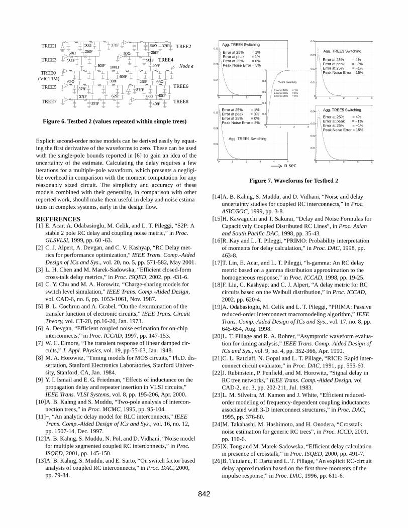
RESULTSThe proposed metrics were tested on several different test bedswhich cover a wide range of topologies, by comparing the stepresponse against a circuit simulator, Spectre. Due to space restric-tions, only the results pertaining to three which illustrate all thecorner cases are shown; the tree of Fig. 3 consisting of the victim,three primary aggressors, and three secondary aggressors (repre-senting an arbitrarily-coupled circuit, where inequality (B) is vio-lated when solving for the poles of the victim switching), thecircuit of Fig. 5 (with far end coupling where inequality (A) is vio-lated when solving for the poles of the aggressor switching), andthe tree of Fig. 6, with four primary and four secondary aggressors(representing global distributed interconnects). Shown in Fig. 4 arethe waveforms at node e of the circuit in Fig. 3, for each driverswitching. It can be seen that the model prediction is very close tothe Spectre simulation. Since the actual and predicted delay at asingle threshold can agree very well, and still result in significantdeviations along the full waveform, we tested the accuracy at threepoints along the waveform. For the victim switching, the thresh-olds are 10%, 50% and 90%, while for the aggressors they are25%, 100% and 25% of the peak amplitude. This is to ensure thatthree points, with two being on either side of the peak, are tested.For the aggressors, the error at different thresholds is given as afraction of the pulse width between the first and last threshold. Thewaveforms for the circuit of Fig. 5 are shown alongside, and thoseof Fig. 6 in Fig. 7.

τ2 R1 CS1 CS2 CS3 CS4 CS5+ + + +( ) R2 CS2 CS3 CS4 CS5+ + +( )+=

τDn

v τDm

v τDm n→

v+=

τ5 R1 CS1 CS2 CS3 CS4 CS5+ + + +( ) R2 CS2 CS3 CS4 CS5+ + +( )R4 CS4 CS5+( ) R5 CS5( )

++ +

=

τ5′

R1 CS1 CS2′

CS3 CS4 CS5+ + + +( ) R2 CS2′

CS3 CS4 CS5+ + +( )

R4 CS4 CS5+( ) R5 CS5( )

+

+ +

=

τ5′ τ5– R1 R2+( ) CS2

′ CS2–( )=

τ5′ τ5 R1 R2+( )+ CS2

′CS2–( )=

840

SUMMARY AND CONCLUSIONSClosed form expressions for the first two moments of the impulseresponse for general arbitrarily-coupled RC trees with multipledrivers were presented, and used to generate stable and accuratesecond order approximations to the transfer function for anyswitching event. The summation of all waveforms results in thecomplete response at the node of interest. These represent newmodels for estimating delay and noise in complex systems, with nocompromise on generality, and in fact subsume a lot of models thataddress simplified structures.

Computing the first two moments of the impulse response of thecircuit, and using them to generate a transfer function with twopoles and one zero results in the matching of boundary conditionsat time zero and infinity, and geometric properties -namely the areaand first moment- of the actual waveform (step response) with theestimated waveform. The boundary conditions are already consid-ered in the particular formulation of the transfer function (i.e. thatthe waveform starts and ends on a specific rail). Hence matchingthe first and second moment of the impulse response does notdefine a unique solution, as a two-pole-one-zero transfer functionhas three unknowns. The necessary third equation is obtained bymatching circuit components to the reciprocal pole sum.

For the switching of the victim driver with the other inputsgrounded, the sum of the open circuit time constants provides agood approximation to the reciprocal pole sum, and combining itwith the moments of the circuit for the victim driver switching hasa straightforward intuitive motivation. For the switching of anaggressor driver, the geometric properties of the actual waveform(via the first and second moments of the impulse response for anaggressor driver switching) are used to obtain the precise recipro-

cal pole sum. Since the quadratic (13) obtained from the momentsof the impulse response for the victim driver switching contain rel-evant information about the victim net, combining it with thereciprocal pole sum for an aggressor switching gives a goodapproximation to the best two-pole-single-zero model. This is aprocedure that works for the vast majority of circuits; howeversome adjustments are necessary to the reciprocal pole sum for cer-tain pathological cases, which was analyzed in a systematic man-ner, resulting in Table 1.

The proposed models have an Elmore-like flavour, and the algo-rithm outlined here allows the moments to be calculated with theabsolute minimum computational effort. However when themoments are computed in a hierarchical manner, starting from thesolution to the DC circuit (a procedure known as path tracing) thesame refinements are possible. Our claim that these models repre-sent the minimum complexity associated with a two-pole-one-zeromodel for this class of circuits is based instead on the fact that thesum of the open circuit time constants is used instead of the thirdmoment, which results in a saving of at least one complete tree tra-versal (or equivalent arithmetic operations). Two moments can beused to map the response to a probability function, but then themodel reverts to a coincident pole transfer function, which reducesthe degree of freedom, or the generality of the model.

For testing purposes, the models we proposed were used to derivethe time domain waveform for the step response. For the delay at agiven threshold, the accuracy was found to be more than 90% onaverage, even for complex circuits such as shown in Fig. 3 and Fig.6. The time at which the peak noise occurs was predicted with evenbetter accuracy. The peak noise itself was predicted with an accu-racy of about 85% or higher in general. These figures cannot beclaimed as being hard bounds for all possible circuit topologies asit is always possible to create a circuit which is poorly representedby a two pole response. However the models did perform very wellwhen tested over a wide range of circuits that are representative ofcoupled interconnect structures in nano-meter technologies.

Figure 3. Testbed 1: arbitrarily-coupled tree

800Ω

150fF600fF

700Ω

300fF

50Ω 150Ω

150fF600fF

450fF

300fF

100Ω 700Ω

300fF 150fF300fF

150fF

800Ω 800Ω

600fF

200Ω

850fF

300fF 1pF

100Ω 400Ω 400Ω 400Ω 400Ω 150Ω 300Ω

300Ω1kΩ

200fF100fF 100fF 100fF 1pF

1pF 1pF

500fF 500fF 500fF1pF

500fF 500fF

2kΩ 1kΩ 1kΩ 1kΩ

10fF

800Ω 700Ω 200Ω600fF 550fF

150fF 300fF 1pF

TREE Ba

TREE B

VICTIM (V)

TREE A

TREE Aa

TREE Ca

TREE C

e

Figure 4. Waveforms for testbed 1 of Figure 3.

Fig.4.b Tree B Switching Fig.4.c Tree A Switching Fig.4.d Tree C SwitchingFig.4.a Victim Switching

0 0.5 1 1.5 2 2.5 3 3.5 4 4.5 5

x 10−8

0

0.1

0.2

0.3

0.4

0.5

0.6

0.7

0.8

0.9

1First Order Response of Victim

Model Simulated

Error at 10% = 3% Error at 50% = 1%Error at 90% = −1%

0 0.5 1 1.5 2 2.5 3 3.5 4 4.5 5

x 10−8

0

0.005

0.01

0.015

0.02

0.025

0.03

0.035Response of Aggressor TREE1

Error at 25% = 3% Error at peak = 1%Error at 25% = −1%Peak Noise Error = 7%

0 0.1 0.2 0.3 0.4 0.5 0.6 0.7 0.8 0.9 1

x 10−7

0

0.002

0.004

0.006

0.008

0.01

0.012

0.014

0.016

0.018Response of Aggressor TREE2

Error at 25% = 2% Error at peak = 2% Error at 25% = 0% Peak Noise Error = 4%

0 0.5 1 1.5 2 2.5 3 3.5 4 4.5 5

x 10−8

0

0.01

0.02

0.03

0.04

0.05

0.06Response of Aggressor TREE3

Error at 25% = 2% Error at peak = 7%Error at 25% = 1%Peak Noise Error = −3%

Figure 5. Example of far-end coupling

e

66Ω69fF 26fF

57fF

100Ω

0 0.2 0.4 0.6 0.8 1 1.2 1.4 1.6 1.8 2

x 10−9

0

0.02

0.04

0.06

0.08

0.1

0.12

0.14

0.16

0.18

0.2

Model Simulated

Error at 25% = 1% Error at peak = 5%Error at 25% = −3%Peak Noise Error = 11%

Aggressor Switching

0 0.2 0.4 0.6 0.8 1 1.2 10

0.1

0.2

0.3

0.4

0.5

0.6

0.7

0.8

0.9

1

Error at 10% = 0% Error at 50% = 0% Error at 90% = 0%

Victim Switching

Component values repeatedwithin simple trees

VICTIM

AGGRESSOR

841

Explicit second-order noise models can be derived easily by equat-ing the first derivative of the waveforms to zero. These can be usedwith the single-pole bounds reported in [6] to gain an idea of theuncertainty of the estimate. Calculating the delay requires a fewiterations for a multiple-pole waveform, which presents a negligi-ble overhead in comparison with the moment computation for anyreasonably sized circuit. The simplicity and accuracy of thesemodels combined with their generality, in comparison with otherreported work, should make them useful in delay and noise estima-tions in complex systems, early in the design flow.

REFERENCES[1] E. Acar, A. Odabasioglu, M. Celik, and L. T. Pileggi, “S2P: A

stable 2 pole RC delay and coupling noise metric,” in Proc. GLSVLSI, 1999, pp. 60 -63.

[2] C. J. Alpert, A. Devgan, and C. V. Kashyap, “RC Delay met-rics for performance optimization,” IEEE Trans. Comp.-Aided Design of ICs and Sys., vol. 20, no. 5, pp. 571-582, May 2001.

[3] L. H. Chen and M. Marek-Sadowska, “Efficient closed-form cross-talk delay metrics,” in Proc. ISQED, 2002, pp. 431-6.

[4] C. Y. Chu and M. A. Horowitz, “Charge-sharing models for switch level simulation,” IEEE Trans. Comp.-Aided Design, vol. CAD-6, no. 6, pp. 1053-1061, Nov. 1987.

[5] B. L. Cochrun and A. Grabel, “On the determination of the transfer function of electronic circuits,” IEEE Trans. Circuit Theory, vol. CT-20, pp.16-20, Jan. 1973.

[6] A. Devgan, “Efficient coupled noise estimation for on-chip interconnects,” in Proc. ICCAD, 1997, pp. 147-153.

[7] W. C. Elmore, “The transient response of linear damped cir-cuits,” J. Appl. Physics, vol. 19, pp-55-63, Jan. 1948.

[8] M. A. Horowitz, “Timing models for MOS circuits,” Ph.D. dis-sertation, Stanford Electronics Laboratories, Stanford Univer-sity, Stanford, CA, Jan. 1984.

[9] Y. I. Ismail and E. G. Friedman, “Effects of inductance on the propagation delay and repeater insertion in VLSI circuits,” IEEE Trans. VLSI Systems, vol. 8, pp. 195-206, Apr. 2000.

[10]A. B. Kahng and S. Muddu, “Two-pole analysis of intercon-nection trees,” in Proc. MCMC, 1995, pp. 95-104.

[11]−, “An analytic delay model for RLC interconnects,” IEEE Trans. Comp.-Aided Design of ICs and Sys., vol. 16, no. 12, pp. 1507-14, Dec. 1997.

[12]A. B. Kahng, S. Muddu, N. Pol, and D. Vidhani, “Noise model for multiple segmented coupled RC interconnects,” in Proc. ISQED, 2001, pp. 145-150.

[13]A. B. Kahng, S. Muddu, and E. Sarto, “On switch factor based analysis of coupled RC interconnects,” in Proc. DAC, 2000, pp. 79-84.

[14]A. B. Kahng, S. Muddu, and D. Vidhani, “Noise and delay uncertainty studies for coupled RC interconnects,” in Proc. ASIC/SOC, 1999, pp. 3-8.

[15]H. Kawaguchi and T. Sakurai, “Delay and Noise Formulas for Capacitively Coupled Distributed RC Lines”, in Proc. Asian and South Pacific DAC, 1998, pp. 35-43.

[16]R. Kay and L. T. Pileggi, “PRIMO: Probability interpretation of moments for delay calculation,” in Proc. DAC, 1998, pp. 463-8.

[17]T. Lin, E. Acar, and L. T. Pileggi, “h-gamma: An RC delay metric based on a gamma distribution approximation to the homogeneous response,” in Proc. ICCAD, 1998, pp. 19-25.

[18]F. Liu, C. Kashyap, and C. J. Alpert, “A delay metric for RC circuits based on the Weibull distribution,” in Proc. ICCAD, 2002, pp. 620-4.

[19]A. Odabasioglu, M. Celik and L. T. Pileggi, “PRIMA: Passive reduced-order interconnect macromodeling algorithm,” IEEE Trans. Comp.-Aided Design of ICs and Sys., vol. 17, no. 8, pp. 645-654, Aug. 1998.

[20]L. T. Pillage and R. A. Rohrer, “Asymptotic waveform evalua-tion for timing analysis,” IEEE Trans. Comp.-Aided Design of ICs and Sys., vol. 9, no. 4, pp. 352-366, Apr. 1990.

[21]C. L. Ratzlaff, N. Gopal and L. T. Pillage, “RICE: Rapid inter-connect circuit evaluator,” in Proc. DAC, 1991, pp. 555-60.

[22]J. Rubinstein, P. Penfield, and M. Horowitz, “Signal delay in RC tree networks,” IEEE Trans. Comp.-Aided Design, vol CAD-2, no. 3, pp. 202-211, Jul. 1983.

[23]L. M. Silveira, M. Kamon and J. White, “Efficient reduced-order modeling of frequency-dependent coupling inductances associated with 3-D interconnect structures,” in Proc. DAC, 1995, pp. 376-80.

[24]M. Takahashi, M. Hashimoto, and H. Onodera, “Crosstalk noise estimation for generic RC trees”, in Proc. ICCD, 2001, pp. 110-6.

[25]X. Tong and M. Marek-Sadowska, “Efficient delay calculation in presence of crosstalk,” in Proc. ISQED, 2000, pp. 491-7.

[26]B. Tutuianu, F. Dartu and L. T. Pillage, “An explicit RC-circuit delay approximation based on the first three moments of the impulse response,” in Proc. DAC, 1996, pp. 611-6.

37fF50Ω25fF

50Ω 37fF

40fF

50Ω

50fF

100Ω

69fF26fF33fF 66Ω

37fF

66Ω 40fF

50fF

50fF

50Ω

62Ω

37fF

37fF 62Ω

37fF 40fF

Figure 6. Testbed 2 (values repeated within simple trees)

TREE1 TREE2

TREE3 TREE4

TREE0(VICTIM)

TREE6

TREE8

TREE5

TREE7

25fF

Node e

0 1 2 3 4 5

x 10−9

0

0.04

0.08

0.12Error at 25% = 1%Error at peak = 3%Error at 25% = 0%Peak Noise Error = 3%

Agg. TREE6 Switching

0 1 2 3 4 5

x 10−9

0

0.04

0.08

0.12Agg. TREE4 Switching

Error at 25% = 1%Error at peak = 1%Error at 25% = 0%Peak Noise Error = 5%

0 1 2 3 4 5

x 10−9

0

0.2

0.4

0.6

0.8

1

Error at 10% = 1%Error at 50% = 0%Error at 90% = 0%

Victim Switching

0 1 2 3 40

0.01

0.02

0.03

0.04

Agg. TREE3 Switching

Error at 25% = 4% Error at peak = −2%Error at 25% = −1%Peak Noise Error = 15%

0 1 2 3 40

0.01

0.02

0.03

0.04 Agg. TREE5 Switching

Error at 25% = 4% Error at peak = −1%Error at 25% = −1%Peak Noise Error = 15%

Figure 7. Waveforms for Testbed 2

n sec

842