analytic number theory - wordpress.com

Analytic Number Theory

Analytic Number Theory

Travis Dirle

December 4, 2016

Contents

1 Summation Techniques 11.1 Abel Summation . . . . . . . . . . . . . . . . . . . . . . . . . 11.2 Euler-Maclaurin Summation . . . . . . . . . . . . . . . . . . . 2

2 Arithmetic Functions 32.1 Arithmetic Functions . . . . . . . . . . . . . . . . . . . . . . . 32.2 The Ring of Arithmetic Functions . . . . . . . . . . . . . . . . 52.3 Important Relationships . . . . . . . . . . . . . . . . . . . . . . 7

3 Dirichlet Series 113.1 Analytic Properties of Dirichlet Series . . . . . . . . . . . . . . 113.2 Euler Products . . . . . . . . . . . . . . . . . . . . . . . . . . . 133.3 Summation Formulae . . . . . . . . . . . . . . . . . . . . . . . 14

4 Average and Extremal Orders 174.1 Average Orders . . . . . . . . . . . . . . . . . . . . . . . . . . 174.2 Extremal Orders . . . . . . . . . . . . . . . . . . . . . . . . . . 19

5 Sieve Methods 215.1 The Sieve of Eratosthenes . . . . . . . . . . . . . . . . . . . . . 215.2 Brun’s Combinatorial Sieve and Twin Primes . . . . . . . . . . 21

6 Characters 236.1 Dirichlet Characters . . . . . . . . . . . . . . . . . . . . . . . . 236.2 Primitive Characters . . . . . . . . . . . . . . . . . . . . . . . 256.3 Gauss Sums . . . . . . . . . . . . . . . . . . . . . . . . . . . . 26

7 Quadratic Reciprocity 297.1 Legendre’s Symbol and its Properties . . . . . . . . . . . . . . 297.2 The Jacobi Symbol . . . . . . . . . . . . . . . . . . . . . . . . 30

8 The Functions ζ(s) and L(s, χ) 338.1 The Zeta Function . . . . . . . . . . . . . . . . . . . . . . . . . 338.2 Approximations and Bounds . . . . . . . . . . . . . . . . . . . 35

i

CONTENTS

8.3 Dirichlet L-functions . . . . . . . . . . . . . . . . . . . . . . . 36

9 The Prime Number Theorem 399.1 Theorems of Chebyshev and Mertens . . . . . . . . . . . . . . 399.2 The Prime Number Theorem . . . . . . . . . . . . . . . . . . . 39

ii

Chapter 1

Summation Techniques

1.1 ABEL SUMMATION

Classically one calls Abel summation (or also partial summation) the processwhereby one transforms a finite sum of products of two terms by means ofthe partial sums of one of them. Thus, by letting A0 = 0, we have An =∑n

m=1 am(n ≥ 1),

N∑n=1

anbn =N∑n=1

(An − An−1)bn =N∑n=1

Anbn −N−1∑n=1

Anbn+1

=N−1∑n=1

An(bn − bn+1) + ANbN .

Theorem 1.1.1. (Abel’s identity) For any arithmetic function a(n) let

A(x) =∑n≤x

a(n),

where A(x) = 0 if x < 1. Assume f has a continuous derivative on the interval[y, x], where 0 < y < x. Then we have∑

y<n≤x

a(n)f(n) = A(x)f(x)− A(y)f(y)−∫ x

y

A(t)f ′(t) dt.

Theorem 1.1.2. Let an∞n=1 be a sequence of complex numbers. Set

A(t) =∑n≤t

an(t > 0).

Let b(t) be a continuously differentiable function on the interval [1, x]. Then wehave ∑

1≤n≤x

anb(n) = A(x)b(x)−∫ x

1

A(t)b′(t) dt.

1

CHAPTER 1. SUMMATION TECHNIQUES

Theorem 1.1.3. (Comparison of a sum and an integral) Let f be a real monotonicfunction on the interval [a, b], with a, b ∈ Z. Then there exists some real numberθ = θ(a, b), 0 ≤ θ ≤ 1, such that∑

a<n≤b

f(n) =

∫ b

a

f(t) dt+ θ(f(b)− f(a))

Theorem 1.1.4. (Second mean value formula) Let f(t) be monotonic and g(t)be integrable on the real interval [a, b]. Then there exists a real number ξ, witha ≤ ξ ≤ b, such that∫ b

a

f(t)g(t) dt = f(a)

∫ ξ

a

g(t) dt+ f(b)

∫ b

ξ

g(t) dt.

1.2 EULER-MACLAURIN SUMMATION

Definition 1.2.1. For any complex x we define the functions Bn(x) by the equa-tion

zexz

ez − 1=∞∑n=0

Bn(x)

n!zn, where |z| < 2π.

The numbersBn(0) are called Bernoulli numbers and are denoted byBn. Thus,

z

ez − 1=∞∑n=0

Bn

n!zn, where |z| < 2π.

Theorem 1.2.2. The functions Bn(x) are polynomials in x given by

Bn(x) =n∑k=0

(n

k

)Bkx

n−k.

Theorem 1.2.3. (Euler-Maclaurin summation formula) For any integer k ≥ 0and for any function f of class Ck+1 on [a, b], a, b ∈ Z, we have∑

a<n≤b

f(n) =

∫ b

a

f(t) dt+k∑r=0

(−1)r+1Br+1

(r + 1)!(f (r)(b)− f (r)(a))

+(−1)k

(k + 1)!

∫ b

a

Bk+1(t)f (k+1)(t) dt.

Theorem 1.2.4. (Euler’s summation formula) If f has a continuous derivative f ′

on the interval [y, x], where 0 < y < x, then∑y<n≤x

f(n) =

∫ x

y

f(t) dt+

∫ x

y

(t− [t])f ′(t) dt

+f(x)([x]− x)− f(y)([y]− y).

2

Chapter 2

Arithmetic Functions

2.1 ARITHMETIC FUNCTIONS

Definition 2.1.1. A real or complex valued function defined on the positive inte-gers is called an arithmetical function or a number-theoretic function.

Definition 2.1.2. A function is called additive if it satisfies

f(mn) = f(m) + f(n) whenever (m,n) = 1;

it is said to be multiplicative if f(1) = 1 and

f(mn) = f(m)f(n) whenever (m,n) = 1;

it is called completely additive or multiplicative if the prior respective condi-tion holds even when (m,n) 6= 1, that is if f(pv) = vf(p) or f(pv) = f(p)v

respectively. One says that f is strongly additive or multiplicative if, besidesprior conditions, f(pv) = f(p) for all v ≥ 1.

Some notation: pv ‖ a means that pv | a but pv+1 - a. The main interestin these notions is that an additive or multiplicative function respects the multi-plicative structure of N∗ in the sense that the image of an integer is the sum orproduct of the images of the prime powers arising in its canonical factorisation.We can thus write

f(n) =∑pv‖n

f(pv), and f(n) =∏pv‖n

f(pv),

when f is respectively additive or multiplicative.Some classical examples of arithmetic functions:• The counting functions of the total number of prime factors of n, taken with

or without multiplicity, respectively:

Ω(n) =∑pv‖n

v and ω(n) =∑pv‖n

1 =∑p|n

1.

3

CHAPTER 2. ARITHMETIC FUNCTIONS

• The divisor function and the sum of kth powers of divisors, denotedrespectively by

τ(n) =∑d|n

1 and σk(n) =∑d|n

dk (k ∈ C).

We have that τ(n) = σ0 and is sometimes denoted d(n). When k = 1, σ1(n)is the sum of the divisors, and is often denoted by σ(n). This function is multi-plicative.• Euler’s totient function is defined to be the number of positive integers

not exceeding n which are relatively prime to n

φ(n) =∑

1≤h≤n,(h,n)=1

1.

• The Mobius function, defined by

µ(n) =

(−1)ω(n), if n is squarefree,0, otherwise.

• The Von Mangoldt’s function

Λ(n) =

log p, if n = pv for some v ≥ 1,

0, if n is not a prime power.

• The identity function given by

δ(n) =

⌊1

n

⌋=

1 if n = 1,

0 if n > 1.

• The unit function denoted u or 1 is the arithemtic function such that u(n) =1 for all n.• Liouville’s function λ is a completely multiplicative function defined by

λ(n) = (−1)Ω(n)

Theorem 2.1.3. The divisor function is multiplicative. We have

τ(n) =∏pv‖n

(v + 1), for (n ≥ 1).

The Mobius function is multiplicative. We have

µ(n) =∏pv‖n

µ(pv).

Theorem 2.1.4. We have that Ω and ω are additive, the former completely, thelatter strongly.

4


2.2 THE RING OF ARITHMETIC FUNCTIONS

Definition 2.2.1. Let f be an arithmetic function. The formal Dirichlet seriesassociated with f is the formal series

D(f ; s) =∞∑n=1

f(n)n−s.

The sum and product of two formal Dirichlet series are defined in a natural wayby

D(f ; s) +D(g; s) =∞∑n=1

(f(n) + g(n))n−s,

D(f ; s)D(g; s) =∞∑n=1

h(n)n−s,

withh(n) =

∑dd′=n

f(d)g(d′).

The set of formal Dirichlet series equipped with these two operations has thestructure of a commutative ring with unity given by the series

D(δ; s) = 1

The correspondence between arithmetic functions and formal Dirichlet seriesinduces on the set of arithmetic functions an addition + and a product ∗ forwhich the fundamental properties are respectively

D(f + g; s) = D(f ; s) +D(g; s)

D(f ∗ g; s) = D(f ; s)D(g; s).

We thus have (f + g)(n) = f(n) + g(n) and (f ∗ g)(n) = h(n) where h is asdefined above.

Definition 2.2.2. The product ∗ is called Dirichlet convolution.

Definition 2.2.3. A necessary and sufficient conditon for an arithmetic f to beinvertible is that f(1) 6= 0. Under this assumption the family of equations∑

d|n

f(n/d)g(d) = δ(n) for (n ≥ 1)

allows us to calculate the inverse function g(n) recursively:g(1) = f(1)−1

g(n) = −f(1)−1∑

d|n,d<n f(n/d)g(d) for (n > 1).

5


Theorem 2.2.4. The group G of units in the ring A of arithmetic functions con-sists of the functions f such that f(1) 6= 0.

Theorem 2.2.5. A necessary and sufficient condition for a function f ∈ A to bemultiplicative is that its associated formal series D(f ; s) be expandable as aninfinite formal product of Eulerian type, that is

D(f ; s) =∏p

(1 +∞∑v=1

f(pv)p−vs).

Theorem 2.2.6. The setM of multiplicative arithmetic functions is a subgroupof the group G of units of A.

Note that the Dirichlet product of two completely multiplicative functionsneed not be completely multiplicative.

Theorem 2.2.7. Let f be multiplicative. Then f is completely multiplicative ifand only if

f−1(n) = µ(n)f(n) for all n ≥ 1.

Theorem 2.2.8. If f is multiplicative, we have∑d|n

µ(d)f(d) =∏p|n

(1− f(p)).

Theorem 2.2.9. (First Mobius inversion formula) Let f and g be arithmetic func-tions. The two following properties are equivalent

(i) g(n) =∑d|n

f(d) for (n ≥ 1)

(ii) f(n) =∑d|n

g(d)µ(n/d) for (n ≥ 1).

The Mobius inversion is really saying g = f ∗ 1⇔ f = g ∗ µ.

Theorem 2.2.10. (Second Mobius inversion formula) Let F and G be functionsdefined on [1,∞]. The following conditions are equivalent

(i) F (x) =∑n≤x

G(x/n) for (x ≥ 1)

(ii) G(x) =∑n≤x

µ(n)F (x/n) for (x ≥ 1).

6


2.3 IMPORTANT RELATIONSHIPS

Theorem 2.3.1. We have that

τ(n) =∑d|n

1 =∑d|n

1(d)1(n/d),

from whichτ = 1 ∗ 1.

Theorem 2.3.2. Let j denote the identity function

j(n) = n for (n ≥ 1).

Then clearly we have σ = 1 ∗ j and also

σk(n) =∑d|n

dk = (1 ∗ jk)(n)

for all real or complex values of the parameter k.

Theorem 2.3.3. The Mobius function is the convolution inverse of the function1, that is

1 ∗ µ = δ.

In other words, ∑d|n

µ(d) =

1 (n = 1)

0 (n > 1).

Theorem 2.3.4. Von Mangoldt’s function can be defined as

Λ = µ ∗ log

or also,Λ = −µ log ∗1.

Theorem 2.3.5. If n ≥ 1 we have

log n =∑d|n

Λ(d).

Definition 2.3.6. (Chebyshev’s summatory functions)

ψ(x) =∑n≤x

Λ(n) = log lcmn : n ≤ x,

θ(x) =∑p≤x

log p

7


Theorem 2.3.7. For x ≥ 1 we have the representation

ψ(x) =∞∑k=1

θ(x1/k)

Definition 2.3.8. We denote by π(x) the number of primes not exceeding x.

Theorem 2.3.9. For x ≥ 2, we have

ψ(x) = θ(x) +O(√x),

π(x) =θ(x)

log x+O

(x

(log x)2

).

Corollary 2.3.10. Let a, b, be constants such that 0 < a < log 2, b > log 4. Forall sufficiently large x, we have

ax ≤ θ(x) ≤ ψ(x) ≤ bx.

Theorem 2.3.11. Euler’s totient function has the following properties:(i) φ(pa) = pa − pa−1

(ii) φ(mn) = φ(m)φ(n)(d/φ(d)), where d = (m,n)(iii) φ(mn) = φ(m)φ(n) if (m,n) = 1(iv) a | b⇒ φ(a) | φ(b)(v) φ(n) is even for n ≥ 3. Moreover, if n has r distinct odd prime factors,

then 2r | φ(n).

Theorem 2.3.12. For each n ≥ 1 we can write the Euler totient function asfollows

φ(n) =∑

1≤m≤n

δ ((m,n)) ,

from which we infer thatφ = µ ∗ j.

In particular for each prime p we have

φ(pv) = µ(1)pv + µ(p)pv−1 = pv(

1− 1

p

).

Theorem 2.3.13. Euler’s totient function is multiplicative. For any integer n ≥1, we have

φ(n) = n∏p|n

(1− 1

p

).

Theorem 2.3.14. We also have that

n =∑d|n

φ(d).

In other words, j = 1 ∗ φ.

8


Theorem 2.3.15. For every n ≥ 1 we have

∑d|n

λ(d) =

1 if n is a square,0 otherwise.

Also, λ−1(n) = |µ(n)| for all n.

9


10

Chapter 3

Dirichlet Series

3.1 ANALYTIC PROPERTIES OF DIRICHLET SERIES

Definition 3.1.1. A Dirichlet series is a series of the form α(s) =∑∞

n=1 ann−s

where s is a complex variable.

Theorem 3.1.2. If β(s) =∑∞

m=1 bmm−s is a second Dirichlet series and γ(s) =

α(s)β(s), then we have that

γ(s) =∞∑k=1

akk−s

∞∑m=1

bmm−s =

∞∑k=1

∞∑m=1

akbm(km)−s =∞∑n=1

(∑km=n

akbm

)n−s.

That is, γ(s) is a Dirichlet series, γ(s) =∑∞

n=1 cnn−s, whose coefficients are

cn =∑km=n

akbm.

The mere convergence of α(s) and β(s) is not sufficient to justify this. It isjustified if the series are absolutely convergent.

Definition 3.1.3. Among the Dirichlet series we shall consider is the Riemannzeta function which for σ > 1 is defined by the absolutely convergent series

ζ(s) =∞∑n=1

n−s.

Definition 3.1.4. We say that a function f(x) is asymptotic to g(x) as x tendsto some limiting value (say x→∞), and write f(x) ∼ g(x), if

limx→∞

f(x)

g(x)= 1.

Definition 3.1.5. We say that f(x) is small oh of g(x) and write f(x) = o(g(x)),if f(x)/g(x)→ 0 as x tends to its limit.

11

CHAPTER 3. DIRICHLET SERIES

Definition 3.1.6. We say that f(x) is big oh of g(x) and write f(x) = O(g(x))if there is a constant C > 0 such that |f(x)| ≤ Cg(x) for all x in the appropriatedomain. The function f may be complex, but g is necessarily non-negative. Wemay also write f(x) g(x).

Definition 3.1.7. If both f g and g f then we say that f and g have thesame order of magnitude, and write f g.

Theorem 3.1.8. Suppose that the Dirichlet series α(s) =∑∞

n=1 ann−s con-

verges at the point s = s0, and H > 0 is an arbitrary constant. Then theseries α(s) is uniformly convergent in the sector S = s : σ ≥ σ0, |t − t0| ≤H(σ − σ0).

Definition 3.1.9. Any Dirichlet series α(s) =∑∞

n=1 ann−s has an abscissa of

convergence σc with the property that α(s) converges for all s with σ > σc, andfor no s with σ < σc. Moreover, if s0 is a point with σ0 > σc, then there is aneighbourhood of s0 in which α(s) converges uniformly.

Theorem 3.1.10. Let A(x) =∑

n≤x an. If σc < 0, then A(x) is a boundedfunction, and

∞∑n=1

ann−s = s

∫ ∞1

A(x)x−s−1 dx

for σ > 0. If σc ≥ 0, then

lim supx→∞

log |A(x)|log x

= σc,

and prior sum holds for σ > σc.

Definition 3.1.11. In general we let σa denote the infimum of those σ for which∑∞n=1 |an|n−σ < ∞. Then σa, the abscissa of absolute convergence, is the

abscissa of convergence of the series∑∞

n=1 |an|n−s, and we see that∑ann

−s

is absolutely convergent if σ > σa, but not if σ < σa. The strip of conditionalconvergence is σc ≤ σ ≤ σa.

Theorem 3.1.12. In the above notation, we have σc ≤ σa ≤ σc + 1.

Remark 3.1.13. We have an interest in Dirichlet series expressed in terms of thesize of |t|. Our interest is in large values of this quantity, but in order that thestatements be valid for small |t| we sometimes write |t|+4, or just let τ = |t|+4.

Theorem 3.1.14. Suppose that α(s) =∑ann

−s has abscissa of convergenceσc. If δ and ε are fixed, 0 < ε < δ < 1, then

α(s) τ 1−δ+ε

uniformly for σ ≥ σc + δ. The implicit constant may depend on the coefficientsan, on δ, and on ε.

12


Theorem 3.1.15. If∑ann

−s =∑bnn

−s for all s with σ > σ0 then an = bn forall positive integers n.

Theorem 3.1.16. (Landau) Let α(s) =∑ann

−s be a Dirichlet series whoseabscissa of convergence σc is finite. If an ≥ 0 for all n then the point σc is asingularity of the function α(s).

3.2 EULER PRODUCTS

Theorem 3.2.1. Let α(s) =∑ann

−s and β(s) =∑bnn

−s be two Dirichletseries, and put γ(s) as their product. If s is a point at which the two series α(s)and β(s) are both absolutely convergent, then γ(s) is absolutely convergent andγ(s) = α(s)β(s).

If f is multiplicative then the Dirichlet series∑f(n)n−s factors into a prod-

uct over primes. To see why, we first argue formally (ignoring questions ofconvergence). When the product∏

p

(1 + f(p)p−s + f(p2)p−2s + f(p3)p−3s + · · · )

is expanded, the generic term is

f(pk11 )f(pk22 ) · · · f(pkrr )

(pk11 pk22 · · · pkrr )s

Set n = pk11 pk22 · · · pkrr . Since f is multiplicative, the above is f(n)n−s. Moreover,

this correspondence between products of prime powers and positive integers nis one-to-one, in view of the fundamental theorem of arithmetic. Hence afterrearranging the terms, we obtain the sum

∑f(n)n−s. That is

∞∑n=1

f(n)n−s =∏p

(1 + f(p)p−s + f(p2)p−2s + · · · ).

Definition 3.2.2. The product on the right-hand side is called the Euler productof the Dirichlet series.

Theorem 3.2.3. If f is multiplicative and∑|f(n)|n−σ < ∞, then

∑f(n)n−s

can be expressed as its Euler product.

13


3.3 SUMMATION FORMULAE

Let

F (s) =∞∑n=1

ann−s

be a Dirichlet series with abscissa of convergence σc and abscissa of absoluteconvergence σa. Extending the definition of the function n 7→ an by settingax = 0 if x ∈ R\N, we introduce the normalized summatory function

A∗(x) =∑n<x

an +1

2ax for x ≥ 0.

Theorem 3.3.1. (Perron’s formula) Let k > max(0, σc). We have

A∗(x) =1

2πi

∫ k+i∞

k−i∞F (s)xss−1 ds for x > 0,

where the integral is conditionally convergent for x ∈ R\N and converges in thesense of Cauchy’s principal value when x ∈ N.

Theorem 3.3.2. (First effective Perron formula) For k > max(0, σa), T ≥ 1and x ≥ 1, we have

A(x) =1

2πi

∫ k+iT

k−iTF (s)xs

ds

s+O

(xk

∞∑n=1

|an|nk(1 + T | log(x/n)|)

).

Corollary 3.3.3. (Second effective Perron formula) Let F (s) =∑∞

n=1 ann−s be

a Dirichlet series with finite abscissa of absolute convergence σa. Suppose thatthere exists some real number α ≥ 0 such that

(i)∞∑n=1

|an|n−σ (σ − σa)−α for (σ > σa),

and that B is a non-decreasing function satisfying(ii) |an| ≤ B(n) for n ≥ 1.Then for x ≥ 2, T ≥ 2, σ ≤ σa, k = σa − σ + 1/ log x, we have∑

n≤x

anns

=1

2πi

∫ k+iT

k−iTF (s+ w)xw

dw

w

+O

(xσa−σ

(log x)α

T+B(2x)

xσ

(1 + x

log T

T

)).

Theorem 3.3.4. For k > max(0, σc) and x ≥ 1, we have∑n≤x

an log(x/n) =1

2πi

∫ k+i∞

k−i∞F (s)xs

ds

s2,

14


and ∫ x

0

A(t) dt =1

2πi

∫ k+i∞

k−i∞F (s)xs+1 ds

s(s+ 1).

15


16

Chapter 4

Average and Extremal Orders

4.1 AVERAGE ORDERS

Definition 4.1.1. Euler’s constant γ is defined by

γ = limn→∞

(n∑k=1

1

k− log n

).

Or also

γ = 1−∫ ∞

1

t− [t]

t2dt

We have γ ≈ 0.577215663.

Definition 4.1.2. We say that an arithmetic function F (n) has a mean value c if

limN→∞

1

N

N∑n=1

F (n) = c.

Definition 4.1.3. We define an average order of an arithmetic function f to beany elementary function g of a real variable such that∑

n≤x

f(n) ∼∑n≤x

g(n).

Theorem 4.1.4. (Dirichlet’s hyperbola method) Let f, g be two arithmetic func-tions, with respective summatory functions F,G. For 1 ≤ y ≤ x, we have∑

n≤x

(f ∗ g)(n) =∑n≤y

g(n)F (x/n) +∑m≤x/y

f(m)G(x/m)− F (x/y)G(y).

Theorem 4.1.5. As x tends to infinity, we have∑n≤x

τ(n) = x(log x+ 2γ − 1) +O(√x)

where γ denotes Euler’s constant.

17

CHAPTER 4. AVERAGE AND EXTREMAL ORDERS


σ(n) =π2

12x2 +O(x log x)


φ(n) =3

π2x2 +O(x log x).


ω(n) = x log2 x+ c1x+O

(x

log x

).

where c1 ≈ 0.261497.


Ω(n) = x log2 x+ c2x+O

(x

log x

)with

c2 = c1 +∑p

1

p(p− 1)≈ 1.034653.

Theorem 4.1.10. The following statements are equivalent:

(i) ψ(x) ∼ x as x→∞,

(ii) M(x) =∑

n≤x µ(n) = o(x) as x→∞,

(iii)∑∞

n=1 µ(n)/n = 0.

(iv) π(x) ∼ x/ log x as x→∞,

(v) θ(x) ∼ x as x→∞,

(vi)∑

n≤x Λ(n)/n = log x− γ + o(1) as x→∞.


µ(n)2 =6

π2x+O(

√x).

18


4.2 EXTREMAL ORDERS

Although the average order of an arithmetic function gives an intuitive idea ofits overall behavior, it can only reflect crudely the variations of its values. Here,we describe standard methods leading to individual bounds that are optimal.

Let f be an arithmetic function. Let g, h denote “elementary” monotone func-tions such as logarithms or powers. The information concerning f may be one ofthe following types:

(i) f(n) = O(g(n)) for (n ≥ n0)(ii) f(n) = o(g(n)) for (n→∞)(iii) f(n) = (1 + o(1))g(n) for (n→∞)(iv) f(n) = g(n) +O(h(n)) for (n ≥ n0).

In the last case it is desirable that h(n) be o(g(n)). A measure of optimal-ity of these asymptotic relations can be expressed by estimates of the followingform (where g(n) is assumed to be ultimately positive):

(a) f(n) = Ω+(g(n)) [i.e. lim sup f(n)/g(n) > 0](b) f(n) = Ω−(g(n)) [i.e. lim inf f(n)/g(n) < 0](c) f(n) = Ω(g(n)) [i.e. lim sup |f(n)|/g(n) > 0].

Definition 4.2.1. Let f be an arithmetic function and let g be a non-decreasingfunction which is ultimately positive. We say that g is a maximal order (resp.minimal order) for f if

lim supn→∞

f(n)/g(n) = 1 (resp. lim infn→∞

f(n)/g(n) = 1).

Theorem 4.2.2. Let f be a multiplicative function. If limpv→∞ f(pv) = 0, thenlimn→∞ f(n) = 0.

Corollary 4.2.3. For all ε > 0 we have τ(n) = Oε(nε).

Theorem 4.2.4. A maximal order for the function log τ(n) is

log 2 · log n/ log2 n.

Theorem 4.2.5. (i) A maximal order for the function ω(n) is log n/ log2 n. (ii)A maximal order for the function Ω(n) is log n/ log 2.

Theorem 4.2.6. A maximal order for φ(n) is n. A minimal order is

e−γn/ log2 n

where γ denotes Euler’s constant.

19


Theorem 4.2.7. For K > 0 a minimal order for σK(n) is nK. For K > 1,a maximal order is ζ(K)nK. For K = 1, a maximal order is eγn log2 n. For0 < K < 1, we have

σK(n) ≤ nK exp

(1 + o(1))

(log n)1−K

(1−K) log2 n

and the opposite inequality is satisfied when n runs through a suitable infinitesequence of integers.

20

Chapter 5

Sieve Methods

5.1 THE SIEVE OF ERATOSTHENES

The sieve of Eratosthenes is a method for counting the numberNm(x) of positiveintegers n not exceeding x that are relatively prime to a fixed number m.

Theorem 5.1.1. (The sieve of Eratosthenes) We have that

Nm(x) =∑d|m∗

(−1)ω(d)[x/d],

where m∗ denotes the square free kernel of m, i.e. m∗ =∏k

j=1 pj , and ω(d)denotes the number of distinct prime factors of d.

Theorem 5.1.2. (Legendre’s formula) We have that

Nm(x) =∑d|m

µ(d)[x/d]

Theorem 5.1.3. When we select m =∏

p≤√x p the only numbers counted by

Nm(x) are 1 and the prime numbers p from the interval [√x, x]. Thus Nm(x) =

π(x)− π(√x) + 1, and we obtain

π(x) = −1 + π(√x) +

∑P+(d)≤

√x

µ(d)[x/d].

5.2 BRUN’S COMBINATORIAL SIEVE AND TWIN PRIMES

Theorem 5.2.1. (Brun) Denote by χt the characteristic function of the set ofintegers n such that ω(n) ≤ t. Then for each integer h ≥ 0 the functions definedby

µi(n) = µ(n)χ2h+2−i(n)

satisfy the inequalities µ1 ∗ 1 ≤ δ ≤ µ2 ∗ 1.

21

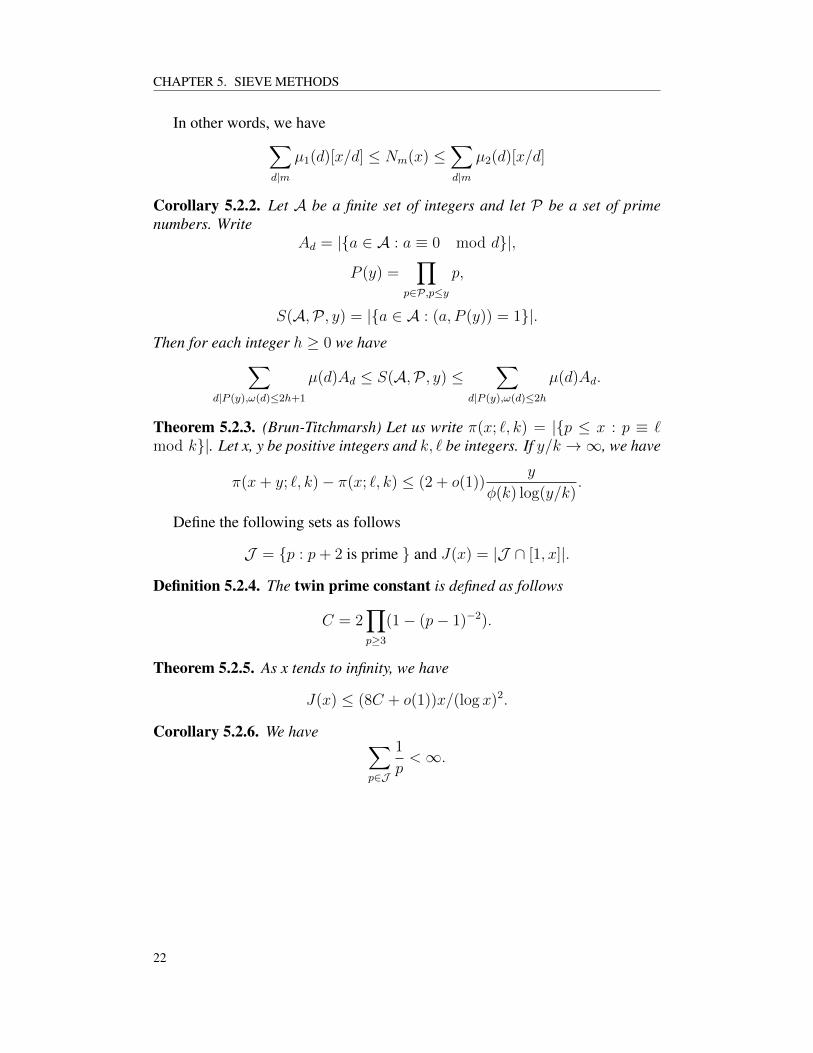
CHAPTER 5. SIEVE METHODS

In other words, we have∑d|m

µ1(d)[x/d] ≤ Nm(x) ≤∑d|m

µ2(d)[x/d]

Corollary 5.2.2. Let A be a finite set of integers and let P be a set of primenumbers. Write

Ad = |a ∈ A : a ≡ 0 mod d|,

P (y) =∏

p∈P,p≤y

p,

S(A,P , y) = |a ∈ A : (a, P (y)) = 1|.Then for each integer h ≥ 0 we have∑

d|P (y),ω(d)≤2h+1

µ(d)Ad ≤ S(A,P , y) ≤∑

d|P (y),ω(d)≤2h

µ(d)Ad.

Theorem 5.2.3. (Brun-Titchmarsh) Let us write π(x; `, k) = |p ≤ x : p ≡ `mod k|. Let x, y be positive integers and k, ` be integers. If y/k →∞, we have

π(x+ y; `, k)− π(x; `, k) ≤ (2 + o(1))y

φ(k) log(y/k).

Define the following sets as follows

J = p : p+ 2 is prime and J(x) = |J ∩ [1, x]|.

Definition 5.2.4. The twin prime constant is defined as follows

C = 2∏p≥3

(1− (p− 1)−2).

Theorem 5.2.5. As x tends to infinity, we have

J(x) ≤ (8C + o(1))x/(log x)2.

Corollary 5.2.6. We have ∑p∈J

1

p<∞.

22

Chapter 6

Characters

6.1 DIRICHLET CHARACTERS

Definition 6.1.1. Let G be an arbitrary group. A complex-valued function χdefined on G is called a character of G if χ has the property

χ(ab) = χ(a)χ(b)

for all a, b ∈ G, and if χ(c) 6= 0 for some c ∈ G.

Theorem 6.1.2. If χ is a character of a finite group G with identity element e,then χ(e) = 1 and each function value χ(a) is a root of unity. In fact, if an = ethen χ(a)n = 1.

Definition 6.1.3. Every group G has at least one character, namely the functionwhich is identically 1 on G. This is called the principal character.

Theorem 6.1.4. A finite abelian group G of order n has exactly n distinct char-acters.

For the remainder of time, G is a finite abelian group of order n. The principalcharacter will be denoted χ0. The other characters have the property that χ(a) 6=1 for some a ∈ G. We use e(θ) to denote e2πiθ.

Theorem 6.1.5. If multiplication of characters is defined by the relation

(χiχj)(a) = χi(a)χj(a)

for each a in G, then the set of characters of G forms an abelian group of order n.We denote this group by G. The identity element of G is the principal characterχ0. The inverse of χi is the reciprocal 1/χi.

Remark 6.1.6. For each character χ we have |χ(a)| = 1. Hence the reciprocal1/χ(a) is equal to the complex conjugate χ(a). Thus the function χ defined byχ(a) = χ(a) is also a character of G. Moreover, we have

χ(a) =1

χ(a)= χ(a−1)

23

CHAPTER 6. CHARACTERS

for every a ∈ G.

Lemma 6.1.7. Suppose that G is cyclic of order n, say G = (a). Then there areexactly n characters of G, namely χk(am) = e(km/n) for 1 ≤ k ≤ n. Moreover,

∑g∈G

χ(g) =

n if χ = χ0,

0 otherwise,

and ∑χ∈G

χ(g) =

n if g = e,

0 otherwise.

In this situation, G is cyclic, G = (χ1).

Theorem 6.1.8. Let G be a finite abelian group. Then G ∼= G, and the previoustwo properties hold.

Definition 6.1.9. A Dirichlet character is a multiplicative homomorphism ofthe group (Z/qZ)∗ into the complex numbers of modulus 1. We extend sucha character to N∗ by setting χ(n) = χ(a) if n ≡ a mod q, (n, q) = 1, andχ(n) = 0 if (n, q) > 1.

Corollary 6.1.10. The multiplicative group (Z/qZ)∗ of reduced residue classesmod q has φ(q) Dirichlet characters. If χ is such a character, then

∑n=1,(n,q)=1

χ(n) =

φ(q) if χ = χ0,

0 otherwise.

If (n, q) = 1, then

∑χ

χ(n) =

φ(q) if n ≡ 1 mod q,

0 otherwise,

where the sum is extended over the φ(q) Dirichlet characters χ mod q.

Theorem 6.1.11. Each Dirichlet character modulo q is completely multiplica-tive with period q. That is, we have

χ(mn) = χ(m)χ(n) for all m,n

andχ(n+ q) = χ(n) for all n

Conversely, if χ is completely multiplicative and periodic with period q, and ifχ(n) = 0 if (n, q) > 1, then χ is one of the Dirichlet characters modulo q.

24


Corollary 6.1.12. If χi is a character mod qi for i = 1, 2, then χ1(n)χ2(n)is a character mod [q1, q2]. If q = q1q2, (q1, q2) = 1, and χ is a charactermod q, then there exist unique characters χi mod q, i = 1, 2, such that χ(n) =χ1(n)χ2(n) for all n.

Theorem 6.1.13. (Orthogonality relations)(i) For all integers n,m ≥ 1, we have

φ(q)−1∑

χ mod q

χ(n)χ(m) =

1 if n ≡ m mod q and (m, q) = 1,

0 otherwise.

(ii) For all Dirichlet characters χ, χ′, to the modulus q, we have

φ(q)−1∑

1≤n≤q

χ(n)χ′(n) =

1 if χ = χ′,

0 otherwise.

6.2 PRIMITIVE CHARACTERS

Definition 6.2.1. Let χ be a Dirichlet character modulo k and let d be any posi-tive divisor of k. The number d is called an induced modulus for χ if we have

χ(a) = 1 whenever (a, k) = 1 and a ≡ 1 mod d.

Definition 6.2.2. Suppose that d | q and that χ∗ is a character modulo d, and set

χ(n) =

χ∗(n) (n, q) = 1

0 otherwise.

Then χ(n) is a Dirichlet character modulo q. In this situation we say that χ∗

induces χ.

Theorem 6.2.3. Let χ be a Dirichlet character modulo k. Then 1 is an inducedmodulus for χ if and only if χ = χ0.

Definition 6.2.4. A Dirichlet character χ mod k is said to be primitive modulok if it has no induced modulus d < k. In other words, χ is primitive modulo kif and only if for every divisor d of k, 0 < d < k, there exists an integer a ≡ 1mod d, (a, k) = 1, such that χ(a) 6= 1.

Theorem 6.2.5. Every nonprincipal character χmodulo a prime p is a primitivecharacter modulo p.

Theorem 6.2.6. Let χ be a Dirichlet character modulo k and assume d | k, d >0. Then d is an induced modulus for χ if and only if

χ(a) = χ(b) whenever (a, k) = (b, k) = 1 and a ≡ b mod d.

25


Definition 6.2.7. Let χ be a Dirichlet character modulo k. The smallest inducedmodulus d for χ is called the conductor of χ.

Theorem 6.2.8. Let χ denote a Dirichlet character modulo q and let d be theconductor of χ. Then d | q, and there is a unique primitive character χ∗ modulod that induces χ.

6.3 GAUSS SUMS

Definition 6.3.1. Given a character χ modulo q, we define the Gauss sum τ(χ)of χ to be

τ(χ) =

q∑a=1

χ(a)e(a/q).

This may be regarded as the inner product of the multiplicative character χ(a)with the additive character e(a/q). The Gauss sum is a special case of the moregeneral sum

cχ(n) =

q∑a=1

χ(a)e(an/q)

When χ is the principal character, this is Ramanujan’s sum

cq(n) =

q∑a=1,(a,q)=1

e(an/q).

Theorem 6.3.2. Suppose that χ is a character modulo q. If (n, q) = 1, then

χ(n)τ(χ) =

q∑a=1

χ(a)e(an/q),

and in particularτ(χ) = χ(−1)τ(χ).

Theorem 6.3.3. Suppose that (q1, q2) = 1, that χi is a character modulo qi fori = 1, 2, and that χ = χ1χ2. Then

τ(χ) = τ(χ1)τ(χ2)χ1(q2)χ2(q1).

Theorem 6.3.4. Suppose that χ is a primitive character modulo q. Then previ-ous theorem holds for all n, and |τ(χ)| = √q.Corollary 6.3.5. Suppose that χ is a primitive character modulo q. Then for anyinteger n,

χ(n) =1

τ(χ)

q∑a=1

χ(a)e(an/q).

26


Theorem 6.3.6. Suppose that χ is a primitive character modulo q with q > 1. Ifχ(−1) = 1, then

L(1, χ) =−τ(χ)

q

q−1∑a=1

χ(a) log(sin πa/q),

while if χ(−1) = −1, then

L(1, χ) =iπτ(χ)

q2

q−1∑a=1

aχ(a).

Theorem 6.3.7. Let χ be a character modulo q that is induced by the primitivecharacter χ∗ modulo d. Then τ(χ) = µ(q/d)χ∗(q/d)τ(χ∗).

27


28

Chapter 7

Quadratic Reciprocity

7.1 LEGENDRE’S SYMBOL AND ITS PROPERTIES

Definition 7.1.1. Given an odd prime p and an integer d relatively prime to p,we define the Legendre symbol as follows:

(dp

)= +1, if d is a quadratic residue mod p,(

dp

)= −1, if d is a non-residue mod p

The multiplicative group F∗p being cyclic of even order p−1, the squares in F∗pform a subgroup (F∗p)2 of index 2 and F∗p/(F∗p)2 is isomorphic to +1,−1. TheLegendre symbol stands for the compositon of the following homomorphisms:

Z→ pZ→ F∗p → F∗p/(F∗p)2 ∼= +1,−1.

As a consequence there is the formula:(ab

p

)=

(a

p

)(b

p

), with a, b ∈ Z− pZ.

Proposition 7.1.2. (Euler’s Criterion) If p is an odd prime and if p - a, then(a

p

)≡ a(p−1)/2 mod p.

Theorem 7.1.3. (The Law of Quadratic Reciprocity) If p and q are distinct oddprime numbers, then (

p

q

)(q

p

)= (−1)(p−1)(q−1)/4.

Proposition 7.1.4. (The Complementary Formulas) If p is an odd prime, then(i)(−1p

)= (−1)(p−1)/2 and

(ii)(

2p

)= (−1)(p2−1)/8.

29

CHAPTER 7. QUADRATIC RECIPROCITY

Proposition 7.1.5. (The First Supplementary Law) Since (p − 1)/2 is even ifp ≡ 1 mod 4 and odd if p ≡ 3 mod 4, then we have(

−1

p

)= (−1)(p−1)/2 =

1 if p ≡ 1 mod 4

−1 if p ≡ 3 mod 4.

Proposition 7.1.6. (The Second Supplementary Law)(2

p

)= (−1)(p2−1)/8

so (2

p

)=

1 if p ≡ ±1 mod 8

−1 if p ≡ ±3 mod 8.

Proposition 7.1.7. (Fermat) Any prime number p ≡ 1 mod 4 may be repre-sented as the sum of two squares.

Theorem 7.1.8. (Lagrange) Every natural number may be represented as thesum of four squares. Hence any prime number is the sum of four squares.

Theorem 7.1.9. If g is a primitive root mod p, then g is a quadratic nonresiduemod p. Consequently, exactly half of the integers 1, 2, . . . , p − 1 are quadraticresidues and half quadratic nonresidues.

Definition 7.1.10. Let K be a field of characteristic 6= p such that K contains thepth roots of unity. Let ζ ∈ K be a primitive pth root of unity. Define the Gausssum by

τp =

p−1∑a=1

(a

p

)ζa.

Theorem 7.1.11. We have that τ 2p = (−1)(p−1)/2p.

7.2 THE JACOBI SYMBOL

Definition 7.2.1. Let Q be an odd positive integer with prime factorization Q =q1 · · · qs. The Jacobi symbol is defined by(

a

Q

)=

s∏i=1

(a

qi

).

It follows directly from the definition that(a

Q

)(a

Q′

)=

(a

QQ′

),

(a

Q

)(a′

Q

)=

(aa′

Q

).

30


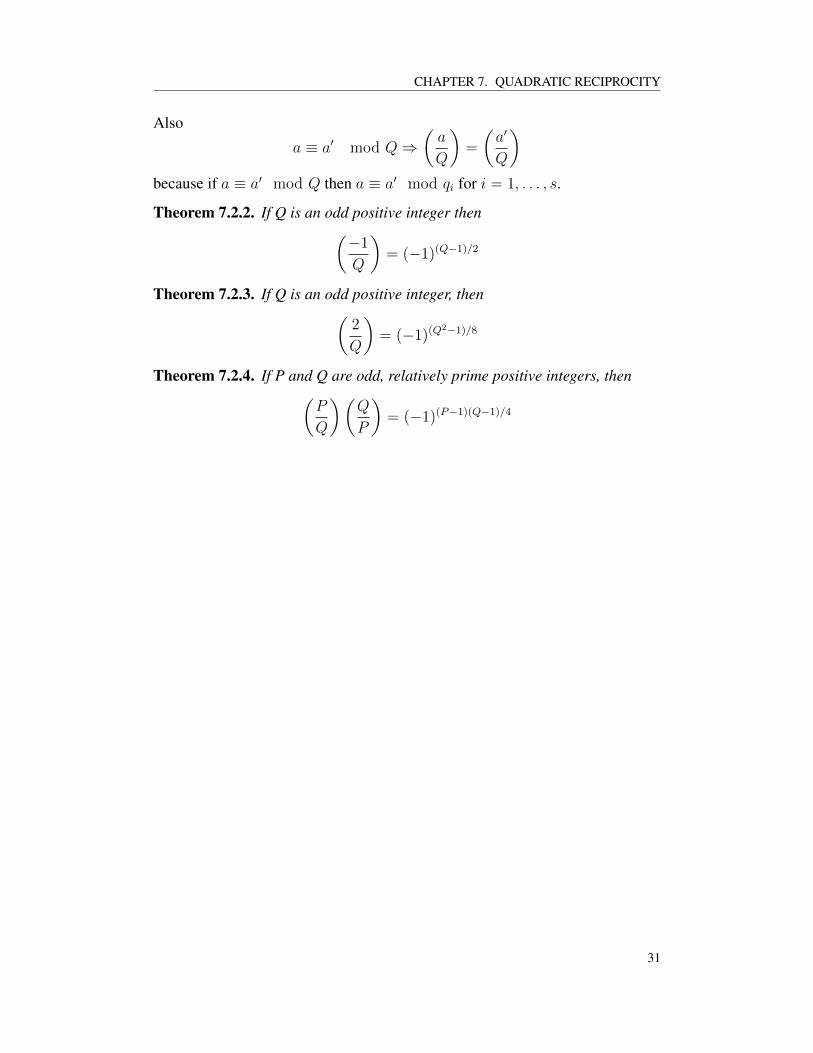
Also

a ≡ a′ mod Q⇒(a

Q

)=

(a′

Q

)because if a ≡ a′ mod Q then a ≡ a′ mod qi for i = 1, . . . , s.

Theorem 7.2.2. If Q is an odd positive integer then(−1

Q

)= (−1)(Q−1)/2

Theorem 7.2.3. If Q is an odd positive integer, then(2

Q

)= (−1)(Q2−1)/8

Theorem 7.2.4. If P and Q are odd, relatively prime positive integers, then(P

Q

)(Q

P

)= (−1)(P−1)(Q−1)/4

31


32

Chapter 8

The Functions ζ(s) and L(s, χ)

8.1 THE ZETA FUNCTION

Definition 8.1.1. The Riemann zeta function, which for σ > 1 is defined by theabsolutely convergent series

ζ(s) =∞∑n=1

n−s

Corollary 8.1.2. For σ > 1, we have∞∑n=1

n−s = ζ(s) =∏p

(1− p−s)−1,

∞∑n=1

µ(n)n−s =1

ζ(s)=∏p

(1− p−s),

∞∑n=1

λ(n)n−s =ζ(2s)

ζ(s)=∏p

(1 + p−s)−1

Also, we have

log ζ(s) =∞∑n=1

Λ(n)

log nn−s

−ζ′(s)

ζ(s)=∞∑n=1

Λ(n)n−s

−ζ ′(s) =∞∑n=1

(log n)n−s

Theorem 8.1.3. Letting Bn denote the nth Bernoulli number, we have

ζ(−n) = (−1)nBn+1

n+ 1for n ≥ 0.

33

CHAPTER 8. THE FUNCTIONS ζ(S) AND L(S, χ)

In particular, ζ(−2n) = 0 for all n ≥ 1.

Definition 8.1.4. The function Γ(s) initially defined for σ > 0 has an ana-lytic continuation to a meromorphic function whose only singularities are sim-ple poles at the negative integers s = 0,−1, . . .. The residue of Γ at s = −n is(−1)n/n!. The gamma function is defined by

Γ(s) =

∫ ∞0

e−tts−1 dt.

Theorem 8.1.5. (The Functional Equation) For each s 6= 1, we have

ζ(s) = 2sπs−1 sin(1

2πs)Γ(1− s)ζ(1− s)

Remark 8.1.6. The functional equation takes the more symmetric form

Φ(s) = Φ(1− s) for s 6= 0, 1

with the notationΦ(s) = π−s/2Γ(s/2)ζ(s).

Theorem 8.1.7. The function ζ(s) is analytically continuable to a meromorphicfunction on the entire complex plane having as sole singularity a simple pole ats = 1, with residue 1.

Theorem 8.1.8. The function ζ(s) has no zero in the half-plane σ ≥ 1. In thehalf plane σ ≤ 0, it has simple zeros at the points −2n(n = 1, 2, . . .).

Definition 8.1.9. The zeros at the negative even integers are called the trivialzeros. The critical stip is where 0 < σ < 1. The non-trivial zeros are thosethat lie in the critical strip.

The functional equation and the fact that ζ(s) is real for real s imply that thezeros are distributed symmetrically with respect to the line σ = 1

2and the real

axis τ = 0.The function (s−1)ζ(s) is entire, but it is more convenient to consider instead

ξ(s) = s(s− 1)π−s/2Γ(s/2)ζ(s) = s(s− 1)Φ(s)

which in addition, satisifes the simpler functional equation

ξ(s) = ξ(1− s)

ξ(s) is an enire function, and not also that ξ(0) = ξ(1) = 1. ξ(s) 6= 0 for σ ≥ 1and for σ ≤ 0. In the critical strip, ξ(s) and ζ(s) have the same zeros.

The general notation for a zero of ξ (i.e. a non-trivial zero of ζ) is ρ = β+ iγ,and we set

N(T ) =∑

ρ:0≤γ≤T

1,

where all zeros ρ are counted with multiplicity.

34


Remark 8.1.10. The Riemann hypothesis conjectures that all non-trivial zerosof ζ(s) lie on the line σ = 1/2. The generalised Riemann hypothesis conjec-tures that all the zeros of L-functions are situated on the critical line σ = 1/2.

8.2 APPROXIMATIONS AND BOUNDS

Corollary 8.2.1. The inequalities

1

σ − 1< ζ(σ) <

σ

σ − 1

holds for all σ > 0. In particular, ζ(σ) < 0 for 0 < σ < 1.

Corollary 8.2.2. Let δ > 0 be fixed. Then

ζ(s) =1

s− 1+O(1)

uniformly for s in the rectangle δ ≤ σ ≤ 2, |t| ≤ 1, and

ζ(s) (1 + τ 1−σ)min

(1

|σ − 1|, log τ

)uniformly for δ ≤ σ ≤ 2, |t| ≥ 1.

Corollary 8.2.3. We have

ζ(1

2+ iτ) |τ |1/6 log |τ | as |τ | → ∞

Theorem 8.2.4. Let a be such that 0 < a < 1. We have

|ζ(s)| ≤ 3|τ |1−a

2a(1− a)for σ ≥ a, |τ | ≥ 1.

In particular, for each positive constant c, we have

ζ(s) log |τ |

for |τ | ≥ 2, σ ≥ 1− c/ log |τ |.

Corollary 8.2.5. For any positive constant c and any integer k ≥ 0, we have

ζ(k)(s) (log |τ |)k+1

for |τ | ≥ 2, σ ≥ 1− c/ log |τ |.

Theorem 8.2.6. For T ≥ 2, we have

N(T + 1)−N(T ) log T

35


Theorem 8.2.7. A T tends to infinity, we have

N(T ) =T

2πlog

T

2π− T

2π+O(log T ).

Theorem 8.2.8. There is an absolute constant c > 0 such that ζ(s) 6= 0 forσ ≥ 1− c/ log τ . This is the classical zero-free region.

Theorem 8.2.9. Let c be the constant in previous theorem. If σ > 1−c/(2 log τ)and |t| ≥ 7/8, then

ζ ′

ζ(s) log τ,

| log ζ(s)| ≤ log log τ +O(1),

and1

ζ(s) log τ.

On the other hand, if 1 − c/(2 log τ) < σ ≤ 2 and |t| ≤ 7/8, then ζ ′/ζ(s) =−1/(s− 1) +O(1), log(ζ(s)(s− 1)) 1, and 1/ζ(s) |s− 1|.

8.3 DIRICHLET L-FUNCTIONS

Definition 8.3.1. For each character χ, with modulos q, the Dirichlet L-seriesis defined by

L(s, χ) =∞∑n=1

χ(n)n−s for σ > 1,

with Euler expansion

L(s, χ) =∏p

(1− χ(p)p−s)−1 for σ > 1.

In particular L(s, χ) 6= 0 when σ > 1. For χ = χ0, the above formula can bewritten as

L(s, χ0) =∑

n=1,(n,q)=1

n−s =∏p|q

(1− p−s)ζ(s).

If χ 6= χ0, then ∑1≤n≤kq

χ(n) = 0

for k = 1, 2, . . . . Hence|∑n≤x

χ(n)| ≤ q.

36


Theorem 8.3.2. If χ 6= χ0, then L(s, χ) is analytic for σ > 0. On the otherhand, the function L(s, χ0) is analytic in this half plane except for a simple poleat s = 1 with residue φ(q)/q. In either case,

logL(s, χ) =∞∑n=2

Λ(n)

log nχ(n)n−s

for σ > 1, and

−L′

L(s, χ) =

∞∑n=1

Λ(n)χ(n)n−s.

Theorem 8.3.3. (Dirichlet) If χ is a character modulo q with χ 6= χ0, thenL(1, χ) 6= 0.

Corollary 8.3.4. (Dirichlet’s theorem) If (a, q) = 1, then there are infinitelymany primes p ≡ a mod q, and indeed∑

p≡a(q)

log p

p=∞.

37


38

Chapter 9

The Prime Number Theorem

9.1 THEOREMS OF CHEBYSHEV AND MERTENS

Theorem 9.1.1. (Chebyshev) For x ≥ 2, we have

x log 2 +O(log x) ≤ ψ(x) ≤ x log 4 +O((log x)2

)Corollary 9.1.2. As x tends to infinity, we have

(log 2 + o(1))x

log x≤ π(x) ≤ (log 4 + o(1))

x

log x.

Theorem 9.1.3. (Bertrand’s Postulate) For every integer n > 3 there is at leastone prime number p such that n < p < 2n− 2.

Theorem 9.1.4. (Merten’s first theorem) We have that∑p≤x

log p

p= log x+O(1)

Theorem 9.1.5. (Merten’s second theorem) We have that∏p≤x

(1− 1/p)−1 = eγ log x+O(1)

9.2 THE PRIME NUMBER THEOREM

Theorem 9.2.1. The prime number theorem says that

π(x) ∼ x

log x

Definition 9.2.2. (Chebyshev’s summatory functions)

ψ(x) =∑n≤x

Λ(n) = log lcmn : n ≤ x,

39

CHAPTER 9. THE PRIME NUMBER THEOREM

θ(x) =∑p≤x

log p

Theorem 9.2.3. For x ≥ 1 we have the representation

ψ(x) =∞∑k=1

θ(x1/k)

Definition 9.2.4. We denote by π(x) the number of primes not exceeding x.

Theorem 9.2.5. For x ≥ 2, we have

ψ(x) = θ(x) +O(√x),

π(x) =θ(x)

log x+O

(x

(log x)2

).

Corollary 9.2.6. Let a, b, be constants such that 0 < a < log 2, b > log 4. Forall sufficiently large x, we have

ax ≤ θ(x) ≤ ψ(x) ≤ bx.

Definition 9.2.7. The logarithmic integral is defined to be

li(x) =

∫ x

2

1

log udu

Theorem 9.2.8. There is a constant c > 0 such that

ψ(x) = x+O

(x

exp(c√

log x)

),

θ(x) = x+O

(x

exp(c√

log x)

),

and

π(x) = li(x) +O

(x

exp(c√

log x)

)uniformly for x ≥ 2.

40

analytic number theory - wordpress.com

Documents