analytic number theory notes - web.stanford.eduaaronlan/assets/analytic-number-theory-notes.pdf ·...
TRANSCRIPT
ANALYTIC NUMBER THEORY NOTES
AARON LANDESMAN
1. INTRODUCTION
Kannan Soundararajan taught a course (Math 249A) on AnalyticNumber Theory at Stanford in Fall 2017.
These are my “live-TeXed“ notes from the course. Conventionsare as follows: Each lecture gets its own “chapter,” and appears inthe table of contents with the date.
Of course, these notes are not a faithful representation of the course,either in the mathematics itself or in the quotes, jokes, and philo-sophical musings; in particular, the errors are my fault. By the sametoken, any virtues in the notes are to be credited to the lecturer andnot the scribe. 1 Please email suggestions to [email protected]
1This introduction has been adapted from Akhil Matthew’s introduction to hisnotes, with his permission.
1

2 AARON LANDESMAN
2. 9/26/17
2.1. Overview. This will be somewhat of an introductory course inanalytic methods, but more like a second introduction. We’ll assumefamiliarity with the prime number theorem, connecting contribu-tions of primes from zeros of the zeta function. You might look at thefirst half of Davenport’s book or so as a prerequisite. We’ll assumethe students know how to prove there are infinitely many primes inarithmetic progressions.
To get started, we’ll do the first four or five lectures proving Vino-gradov’s three prime theorem:
Theorem 2.1 (Vinogradov). Every large odd number is the sum of threeprimes.
When we say “large,” one can actually compute the bound explic-itly (i.e., it is effective).
Remark 2.2. Helfgott, a few years back, made the bound accessibleso that one could compute exactly which odd numbers were not ex-pressible as the sum of three primes. He showed something like allprimes more than 7 could be written as the sum of three primes.
To start the proof, write N = p1 + p2 + p3, and we’ll count thenumber of ways to write N as such. In fact, we’ll consider
∑N=n1+n2+n3
Λ(n1)Λ(n2)Λ(n3)
where
Λ(n) :=
{log p if n = pk
0 else
If we define
Ψ(x) := ∑n≤x
Λ(n) = x + O(xe−c√
log x).
This is equivalent to saying
π(x) = li(x) + o(xe−c√
log x).
Here
li(x) =∫ x
2
dtlog t
.
li(x) is about xlog x .
ANALYTIC NUMBER THEORY NOTES 3
2.2. Heuristic of proof. A first guess is that there are about π(N)choices for each of p1, p2, p3. Their sum must add up to a given num-ber N. The chance that p1 + p2 + p3 is exactly N is roughly 1
N . Hence,the number of such ways is approximately(
Nlog N
)3 1N
=N2
(log N)3 .
We can also estimate
R3(N) := ∑N=n1+n2+n3
Λ(n1)Λ(n2)Λ(n3) ∼ N3/N = N2 + O(N1+1/2 + log N)
where the error comes from contributions of powers of primes.
2.3. Hardy and Littlewood’s circle method. Let
S(α) := ∑n≤N
Λ(n)e(nα)
where
e(x) = e2πix.
Then,∫ 1
0S(α)3e(−Nα)dα =
∫ 1
0∑
n1,n2,n3≤NΛ(n1)Λ(n2)Λ(n3)e (n1 + n2 + n3 − N)α) dα
= R3(N).
To bound this, note that S(0) = Ψ(N) ∼ N. We’d like to bound it byabout N2.
Also, S(1/2) is pretty big because
S(1/2) = (Λ(2) + λ(4) + · · · )− ∑n≤N,n odd
Λ(n)
because e(x) = −1 if x is odd.Then, for all
|λ| ≤ 10−6
N,
we have <S(α) > .99N. Then,∫|α|≤10−6/N
S(α)3e(−Nα)dα ' 10−6N2.
We could similarly make an argument in a small neighborhood of12 . This gives an analytic reason that the number of representationsmight be on the scale of N2. So there are portions of the integralwhich give the correct answer.
4 AARON LANDESMAN
Exercise 2.3 (Waring’s problem). We want to know whether we canwrite N = xk
1 + xk2 + · · ·+ xk
3 (i.e., as a sum of four squares or ninecubes, etc.)
(1) First, find a probabilistic guess for the number of such repre-sentations.
(2) Use the circle method
∫ 1
0
∑n≤N
1k
e(nkα)
S
e(−Nα)dα.
Then, find portions of the integrand that correspond to theright probabilistic answer.
Returning to our integral for three primes, let’s think about whenS(α) is big.
Example 2.4. Let’s try 13 .
∑n≤N
Λ(n)e(n/3).
We have a contribution from powers of 3 which is about log N, so
∑n≤N
Λ(n)e(n/3) = O(log N) + e(1/3)Ψ(N; 3, 1) + e(2/3)Ψ(N; 3, 2)
∼ N/2.
where
Ψ(N; 3, 1) ∼ Nφ(3)
=N2
.
where Ψ(N; a, b) counts the number of primes up to N which isb mod a.
Remark 2.5. Note that
S(aq)
counts approximately the distribution of primes in progressions modq with (a, q) = 1. Sometimes when q is small, since we’re only countprimes coprime to q, we will get an answer substantially away from0.
We’ll later need to think through the uniformity of q in terms of N.
ANALYTIC NUMBER THEORY NOTES 5
Remark 2.6 (Insight). S(α) is big near most rational numbers withsmall denominators. It’s not big near 1/4, so we’re only saying it’sbig near certain ones. This might have something to do with whetherthe denominator of the rational number is square free: if it is notsquare free, you essentially get translates over roots of unity of thatprime whose square divides q, and things cancel out
Exercise 2.7. Show∗∑
k mod qe(
akq) = µ(q),
where the ∗means (k, q) = 1 and µ is the Mobius function.
Goal 2.8. If α is not near a rational number with small denominatorthen |S(α)| is small.
To accomplish this, Hardy and Littlewood decided to split [0, 1]into two parts - major arcs M and minor arcs m. The major arcs areclose to a
q for q small, and the minor arcs are the rest. The measure ofthe minor arcs are big while the measure of the major arcs have smallmeasure. That is, the minor arcs have nearly full measure. So, thereis a very small set on which the generating function is big. There isalso a big set on which the generating function is small.
There is a trivial bound |S(α)| ≤ Ψ(N) ∼ N, using the triangleinequality. One can also work out
Lemma 2.9. We have ∫ 1
0|S(α)|2dα ∼ N log N.
Proof. ∫ 1
0|S(α)|2dα = ∑
n1,n2≤NΛ(n1)Λ(n2)
∫ 1
0e ((n1 − n2)α) dα
= ∑n≤N
Λ(n)2
= ∑n≤N
log nΛ(n) + O(√
N log N)
= N log N.
Exercise 2.10. Verify the above, where the O(√
N log N) differenceis coming from prime powers. The idea for the last step is that most
6 AARON LANDESMAN
numbers less than N are on the order of N. One might use partialsummation, which is integration by parts.
�
Usually,
|S(α)| ∼√
N log N.
If α is far from every rational number, such as the golden ratio, φ,we might try to compute S(φ). We might expect that S(φ) � N
12+ε.
We don’t know whether this is true, but we do know
∑n≤N
Λ(n)e(nφ)� N1−δ
for some δ > 0 (and it will probably even be a pretty large δ). We willnow develop a technique saying that once you are far away from arational number, you can get this sort of power saving.
2.4. Strategy for determining asymptotics for R3(N). We have theintegral ∫ 1
0S(α)3e(−Nα)dα = (
∫M+∫
m)S(α)3e(−Nα)dα
We want the second part over the minor arcs to be smaller than N2.The idea is that we can bound∣∣∣∣∫m
S(α)3e(−Nα)dα
∣∣∣∣ ≤(
∑α∈m|S(α)|
) ∫ 1
0|S(α)|2dα
� (N log N)∑m|S(α)|.
So, it is enough to have
∑α∈m|S(α)| ≤ εN
log N.
This will show the contribution from the minor arcs is less than thatof the major arcs, assuming we know the major arcs contribute N2.
Exercise 2.11 (Roth). For all δ > 0, there is N0 = N(δ) so that for allN ≥ N0, such that every subset A ⊂ [1, N] with |A | ≥ δN has a(nontrivial) three term arithmetic progression.
Letting
A (α) = ∑a∈A
e(aα),
ANALYTIC NUMBER THEORY NOTES 7
we obtain ∫ 1
0A (α)2A (−2α)dα
counts the number of triples (x, y, z) with x + z = 2y. This includes|A | trivial solutions, so we want to see this integral is larger. Wemight expect δ3N2 solutions. But now, it’s a bit hard to see how toactually bound this integral.
Exercise 2.12 (Vague exercise). If, “away from 0,”
|A (α)| ≤ ε|A |then the contribution of that portion of the integral∫ 1
0A (α)2A (−2α)dα
is bounded by ε|A |2. (We’d like to know something like ε ≤ δ/106.)
The idea is that either we have this bound above, or else we getsome additive structure in A which we exploit to get a bigger den-sity set.
There are notes on this on Sound’s web-page from a course hetaught on additive combinatorics.
Now, we want to focus on showing that for some definition of theminor arcs, the sum S(α) has a little bit of cancellation.
2.5. Vinogradov’s method. Here is the key idea from Vinogradov’smethod. This comes up many times throughout analytic numbertheory. We’d like to understand the sequence
S(α) = ∑n≤N
Λ(n)e(nα).
We could similarly study
∑n≤N
Λ(n)e( f (n)),
where, say, f (n) is e(√
n) or e(√
n + (log n)2). We could similarlystudy
∑n≤N
e(√
n)
or
∑n≤N
e(t log n)
8 AARON LANDESMAN
for looking at 0’s of the zeta function. Let’s start with the simplestversion of these, where instead of summing over primes and primepowers, we only sum over all the integers. Say we want to consider
∑n≤N
e(nα).
This is a geometric progression, so it is easy to sum:
∑n≤N
e(nα) =e(α) (1− e(Nα))
1− e(α)
=x
sin πα
where x is bounded by 2, and the numerator is approximately sin πNα.
Exercise 2.13. Show∣∣∣∣∣ ∑n≤N
e(nα)
∣∣∣∣∣ ≤ min(
N,2
sin πα
)� min
(N,
1||α||
).
letting ||α|| denote the distance from the nearest integer.
Let Φ be a smooth function. Then,
∑n
Φ(n/N)e(nα)
is some smooth version of what we are trying to approximate. Wemight try to use the Poisson summation formula. We can write
∑n
Φ(n/N)e(nα) = N ∑k
φ(N(k + α))
and work out the Poisson summation formula. For φ smooth, theFourier transform is rapidly decreasing.
3. 9/28/17
Recall last time we had
R3(N) := ∑n1+n2+n3=N
Λ(n1)Λ(n2)Λ(n3).
The goal was to show this asymptotes to N2. We set
S(α) = ∑n≤N
Λ(n)e(nα),
ANALYTIC NUMBER THEORY NOTES 9
and found
R3(N) =∫ 1
0S(α)3e(−Nα)dα.
The idea is to show that S(α) is large only near rational numberswith small denominators (the minor arcs). On the complement, wewant to show |S(α)| is small, and then bound
|∫
mS(α)3e(−Nα)dα| ≤
(supα∈m|S(α)|
) ∫ 1
0|S(α)|2dα.
We then could use Parseval’s identity to bound this by N log N.Toward the end of last time, we found
∑n≤N
e(nα)� min(N,1||α|| ).
Exercise 3.1. Count the number of ways of writing N = n1 + n2 +n3 asymptotically by writing down the associated integral using thecircle method. The exponential sum will only be big for α near 0.There is only one major arc in this case. The answer should be aboutN2/2, and the point is to see where the 1/2 comes from.
Recall from elementary number theory that Λ(n) = ∑ab=n µ(a) log b.If we look at the Dirichlet series for
−ζ ′
ζ(s) =
1ζ(s)
· −ζ ′(s)
where the first term has Dirichlet series Λ(n), 1ζ has Dirichlet series
µ and −ζ ′(s) has Dirichlet series log. Then, the convolution of µ andlog is Λ. Then,∫
n≤Nlog ne(nα) =
∫ N
1−log td
(∑n≤t
e(nα)
)
= log N ∑n≤N
e(nα)−∫ N
1−
1t ∑
n≤te(nα)dt
� (log N)min(
N,1||α||
).
Then,
∑n≤N
Λ(n)e(nα) = ∑a
µ(a) ∑b≤N/a
log be(abα).
10 AARON LANDESMAN
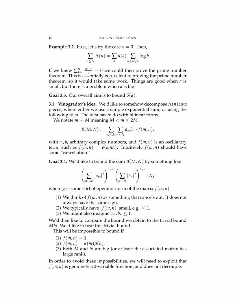
Example 3.2. First, let’s try the case α = 0. Then,
∑n≤N
Λ(n) = ∑a
µ(a) ∑b≤N/a
log b
If we knew ∑∞a=1
µ(a)a = 0 we could then prove the prime number
theorem. This is essentially equivalent to proving the prime numbertheorem, so it would take some work. Things are good when a issmall, but there is a problem when a is big.
Goal 3.3. Our overall aim is to bound S(α).
3.1. Vinogradov’s idea. We’d like to somehow decompose Λ(n) intopieces, where either we use a simple exponential sum, or using thefollowing idea. The idea has to do with bilinear forms.
We notate m ∼ M meaning M < m ≤ 2M.
B(M, N) := ∑m∼M
∑n∼N
ambn · f (m, n),
with ai, bi arbitrary complex numbers, and f (m, n) is an oscillatoryterm, such as f (m, n) = e(mnα). Intuitively f (m, n) should havesome “cancellation.”
Goal 3.4. We’d like to bound the sum B(M, N) by something like(∑
m∼M|am|2
)1/2(∑
n∼N|bn|2
)1/2
· N f
where g is some sort of operator norm of the matrix f (m, n).
(1) We think of f (m, n) as something that cancels out. It does notalways have the same sign.
(2) We typically have | f (m, n)| small, e.g., ≤ 1.(3) We might also imagine am, bn ≤ 1.
We’d then like to compare the bound we obtain to the trivial boundMN. We’d like to beat this trivial bound.
This will be impossible to bound if(1) f (m, n) = 1.(2) f (m, n) = α(m)β(n).(3) Both M and N are big (or at least the associated matrix has
large rank).In order to avoid these impossibilities, we will need to exploit thatf (m, n) is genuinely a 2-variable function, and does not decouple.

ANALYTIC NUMBER THEORY NOTES 11
To obtain the bound, we will use Cauchy-Schwarz. We have∣∣∣∣∣ ∑m∼M
∑n∼N
ambn f (m, n)
∣∣∣∣∣2
≤(
∑m∼M
|am|2) ∑
m∼M
∣∣∣∣∣ ∑n∼N
bn f (m, n)
∣∣∣∣∣2 .
Let ∗ denote
∑m∼M
∣∣∣∣∣ ∑n∼N
bn f (m, n)
∣∣∣∣∣2
Then,
∗ = ∑m∼M
∣∣∣∣∣ ∑n∼N
bn f (m, n)
∣∣∣∣∣2
≤ ∑n1,n2∼N
bn1bn2 ∑m∼M
f (m, n1) f (m, n2).
From this we have gained that we have replaced the unknown am, bnby inner products of our known matrix f (m, n).
If we knew f (m, n) were orthogonal, then the sum amounts toterms with n1 = n2 of the form
∑n∼N|bn|2M.
Things will never be quite so good that we will precisely get orthog-onality. But, we might have some approximate orthogonality. Forexample, if n1 6= n2, maybe we can bound the correlation by 1. Then,the off-diagonal terms are of the form
∑n1 6=n2
|bn1bn2 .
Using Cauchy’s inequality, we obtain
|bn1bn2 | � |bn1 |2 + |bn2 |2.
Hence,
∑n1 6=n2
|bn1bn2 � N ∑n∼N|bn|2.
In the above favorable circumstances, putting the above together, weget a bound∣∣∣∣∣ ∑m∼M
∑n∼N
ambn f (m, n)
∣∣∣∣∣�(
∑m∼M
|am|2)1/2(
∑n∼N|bn|2
)1/2 (√M +
√N)
12 AARON LANDESMAN
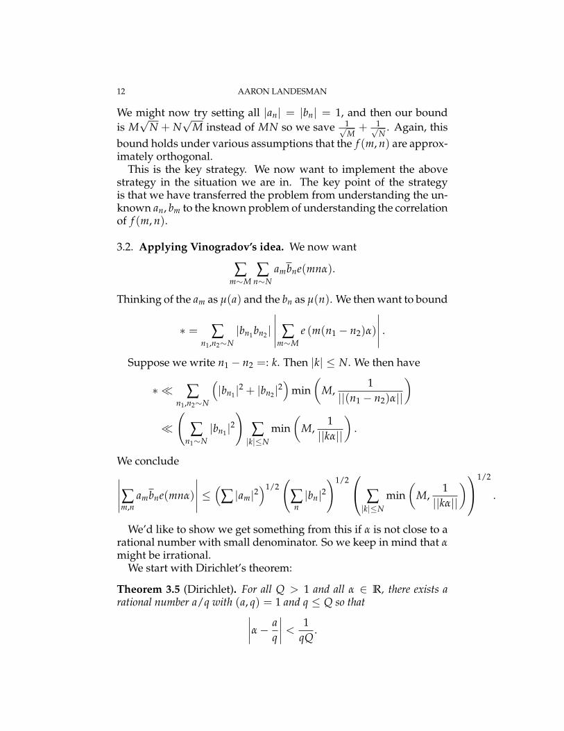
We might now try setting all |an| = |bn| = 1, and then our boundis M√
N + N√
M instead of MN so we save 1√M+ 1√
N. Again, this
bound holds under various assumptions that the f (m, n) are approx-imately orthogonal.
This is the key strategy. We now want to implement the abovestrategy in the situation we are in. The key point of the strategyis that we have transferred the problem from understanding the un-known an, bm to the known problem of understanding the correlationof f (m, n).
3.2. Applying Vinogradov’s idea. We now want
∑m∼M
∑n∼N
ambne(mnα).
Thinking of the am as µ(a) and the bn as µ(n). We then want to bound
∗ = ∑n1,n2∼N
|bn1bn2 |∣∣∣∣∣ ∑m∼M
e (m(n1 − n2)α)
∣∣∣∣∣ .
Suppose we write n1 − n2 =: k. Then |k| ≤ N. We then have
∗ � ∑n1,n2∼N
(|bn1 |
2 + |bn2 |2)
min(
M,1
||(n1 − n2)α||
)
�(
∑n1∼N
|bn1 |2
)∑|k|≤N
min(
M,1||kα||
).
We conclude∣∣∣∣∣∑m,nambne(mnα)
∣∣∣∣∣ ≤ (∑ |am|2)1/2
(∑n|bn|2
)1/2 ∑|k|≤N
min(
M,1||kα||
)1/2
.
We’d like to show we get something from this if α is not close to arational number with small denominator. So we keep in mind that αmight be irrational.
We start with Dirichlet’s theorem:
Theorem 3.5 (Dirichlet). For all Q > 1 and all α ∈ R, there exists arational number a/q with (a, q) = 1 and q ≤ Q so that∣∣∣∣α− a
q
∣∣∣∣ < 1qQ
.
ANALYTIC NUMBER THEORY NOTES 13
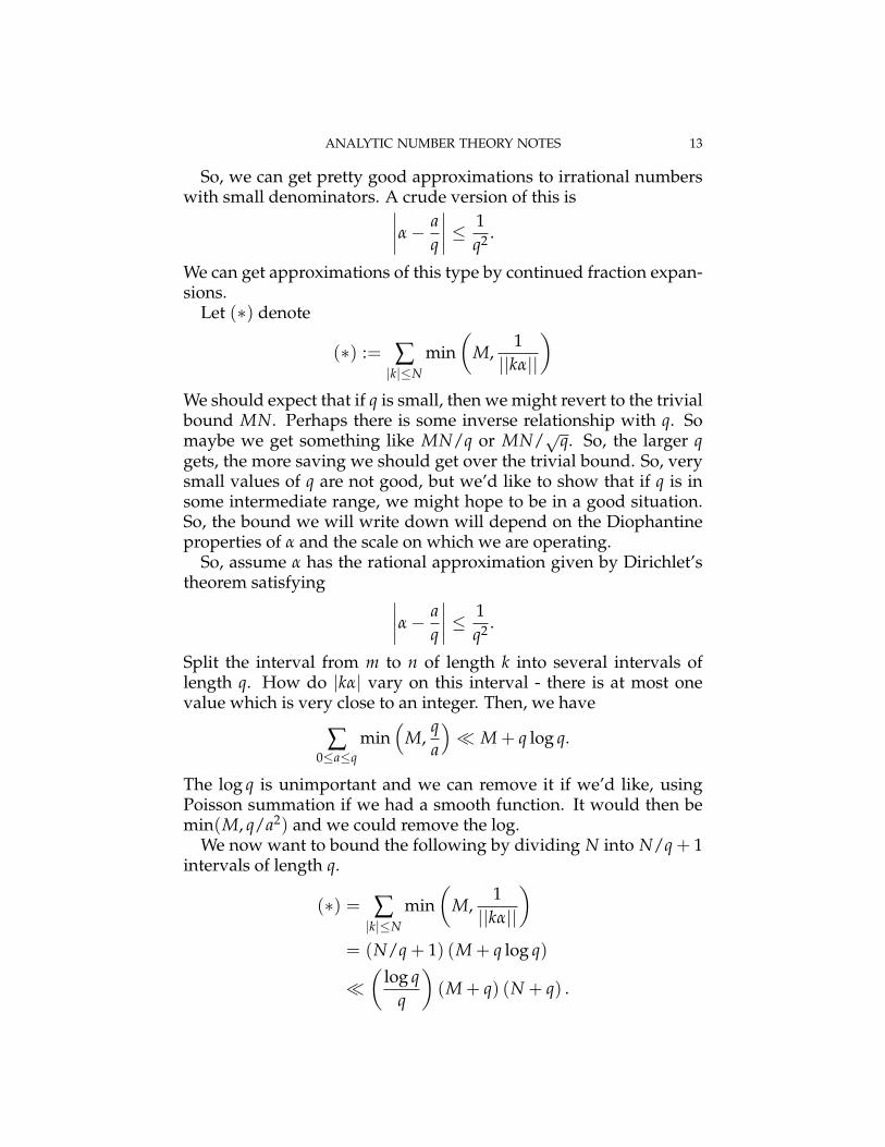
So, we can get pretty good approximations to irrational numberswith small denominators. A crude version of this is∣∣∣∣α− a
q
∣∣∣∣ ≤ 1q2 .
We can get approximations of this type by continued fraction expan-sions.
Let (∗) denote
(∗) := ∑|k|≤N
min(
M,1||kα||
)We should expect that if q is small, then we might revert to the trivialbound MN. Perhaps there is some inverse relationship with q. Somaybe we get something like MN/q or MN/
√q. So, the larger q
gets, the more saving we should get over the trivial bound. So, verysmall values of q are not good, but we’d like to show that if q is insome intermediate range, we might hope to be in a good situation.So, the bound we will write down will depend on the Diophantineproperties of α and the scale on which we are operating.
So, assume α has the rational approximation given by Dirichlet’stheorem satisfying ∣∣∣∣α− a
q
∣∣∣∣ ≤ 1q2 .
Split the interval from m to n of length k into several intervals oflength q. How do |kα| vary on this interval - there is at most onevalue which is very close to an integer. Then, we have
∑0≤a≤q
min(
M,qa
)� M + q log q.
The log q is unimportant and we can remove it if we’d like, usingPoisson summation if we had a smooth function. It would then bemin(M, q/a2) and we could remove the log.
We now want to bound the following by dividing N into N/q + 1intervals of length q.
(∗) = ∑|k|≤N
min(
M,1||kα||
)= (N/q + 1) (M + q log q)
�(
log qq
)(M + q) (N + q) .
14 AARON LANDESMAN
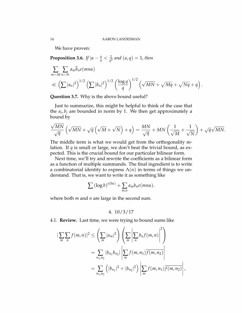
We have proven:
Proposition 3.6. If |α− aq < 1
q2 and (a, q) = 1, then
∑m∼M
∑n∼N
ambne(mnα)
�(∑ |an|2
)1/2 (∑ |bn|2
)1/2(
log qq
)1/2 (√MN +
√Mq +
√Nq + q
).
Question 3.7. Why is the above bound useful?
Just to summarize, this might be helpful to think of the case thatthe ai, bj are bounded in norm by 1. We then get approximately abound by√
MN√
q
(√MN +
√q(√
M +√
N)+ q)=
MN√
q+ MN
(1√M
+1√N
)+√
q√
MN.
The middle term is what we would get from the orthogonality re-lation. If q is small or large, we don’t beat the trivial bound, as ex-pected. This is the crucial bound for our particular bilinear form.
Next time, we’ll try and rewrite the coefficients as a bilinear formas a function of multiple summands. The final ingredient is to writea combinatorial identity to express Λ(n) in terms of things we un-derstand. That is, we want to write it as something like
∑ (log b)e(bα) + ∑m,n
ambne(mnα).
where both m and n are large in the second sum.
4. 10/3/17
4.1. Review. Last time, we were trying to bound sums like
|∑m
∑n
f (m, n)|2 ≤(
∑m|am|2
)∑m
∣∣∣∣∣∑nbn f (m, n)
∣∣∣∣∣2
= ∑n1,n2
|bn1bn2 |∣∣∣∣∣∑m f (m, n1) f (m, n2)
∣∣∣∣∣= ∑
n1,n2
(|bn1 |
2 + |bn2 |2) ∣∣∣∣∣∑m f (m, n1) f (m, n2)
∣∣∣∣∣ ,
ANALYTIC NUMBER THEORY NOTES 15
and we hoped that the correlations, i.e., the terms∣∣∣∑m f (m, n1) f (m, n2)
∣∣∣were bounded by M if n1 = n2 and O(1) if n1 6= n2. We then couldbound the above by (M + N)∑i |bn|2.
Recall last time, we were trying to bound sums like
∑m∼M
∑n∼N
ambne(mnα)
where m ∼ M means M ≤ m ≤ 2M. We had∣∣∣∣α− aq
∣∣∣∣ ≤ 1q2 ,
with (a, q) = 1. We proved last time
∑m∼M
∑n∼N
ambne(mnα)
� log q√
q
(∑m|am|2
)1/2(∑n|bn|2
)1/2 (√MN +
√q(√
M +√
N)+ q)
.
We had
Λ(n) = ∑ µ(a) log b
S(α) = ∑n≤N
Λ(n)e(nα).
Our tools are(1)
∑n≤x
log ne(nα)
is some sort of geometric progression which after factoringout a log, which we understand
(2)
∑m∼M
∑n∼N
ambne(mnα)
which is well bounded using Vinogradov’s method discussedlast time (and above this lecture) assuming the covariancesare small for off-diagonal terms and on the order of the num-ber of elements for the diagonal terms.
Our goal is now the following combinatorial one:
Goal 4.1. Write Λ(n) in a form where we can use the above two tools.
16 AARON LANDESMAN
Theorem 4.2 (Vaughan’s identity). We have
∞
∑n=1
Λ(n)ns = −ζ ′
ζ(s)
1ζ(s)
= ∑a
µ(a)as
−ζ ′(s) = ∑b
log bbs .
Proof. This follows from straightforward manipulations of Dirichletseries, the first one comes from the derivative of log ζ(s). �
4.2. Mollifying ζ(s). We now want to Mollify ζ(s). For this, we willuse Selberg’s sieve.
One way to study the zeta function could be an appropriate trun-cation. We may consider
M(s) = ∑n≤U
µ(n)ns .
which is a sort of approximation to the inverse of the Riemann ζfunction, using the above identity that
1ζ(s)
= ∑a
µ(a)as
One can compute,
ζ(s)M(s) =∞
∑n=1
a(n)ns .
where a(n) is defined by
a(n) = ∑d|n,d≤U
µ(d)
=
1 if n = 10 if 1 < n ≤ Uthe norm is bounded by d(n) if n > U
where d(n) is the number of divisors of n.
ANALYTIC NUMBER THEORY NOTES 17
We have
−ζ ′
ζ(s) = −ζ ′
ζ(s) (1− ζM + ζM)
= −ζ(s)M(s)− ζ ′
ζ(s) (1− ζM(s)) .
First, we should be fairly happy with the term −ζ(s)M(s) whichhas Dirichlet series given by(
∑log b
bs
)(∑
n≤U
M(n)ns
),
and we’ll have a long sum in the b’s, where we can hope to get somecancellation. Next, to understand
ζ ′
ζ(s) (1− ζM(s)) .
We try to think of this product as a sort of bilinear form. The termsfrom 1 − ζM(s) only matter for n larger than U. Thinking of thisterm as a bilinear term, we’re happy because 1− ζM(s) is large. But,we have to ensure that ζ ′/ζ is not too “skinny.” To deal with this, wecan subtract out the small primes, and then later add them back.
To accomplish this, we define
P(s) := ∑n≤V
Λ(n)ns .
Then,
−ζ ′
ζ(s) = −ζ ′
ζ(s)− P(s) + P(s)
= ∑n>V
Λ(n)ns + ∑
n≤V
Λ(n)ns
Then,
−ζ ′
ζ(s) = −ζ ′(s)M(s)− ζ ′
ζ(s) (1− ζM(s))
= −ζ ′(s)M(s) +(−ζ ′
ζ(s)− P(s)
)(1− ζM(s)) + P(s) (1− ζM(s))
= −ζ ′(s)M(s) +(−ζ ′
ζ(s)− P(s)
)(1− ζM(s)) + P(s)− ζ(s)M(s)P(s)
18 AARON LANDESMAN
The point of this breakdown is that we now have three terms we canhandle using our two tools we have.
The middle term decomposes into two parts, both of which arebig, which gives a bilinear form.
The last term has a long sum from the ζ(s) term in simple coeffi-cients. For P(s), we can just ignore it because V is small. The firstterm is similarly a long some from the ζ ′ term.
Remark 4.3. The first term which we handle via our first summationtechnique is called a “type 1 sum” and the second handled via oursecond bilinear form summation technique is called a “type 2 sum.”
Example 4.4. Let’s say we want to write
−ζ ′
ζ(s) =
−ζ ′
ζ(s)((1− ζM)2 + 2ζM− ζ2M2
)=
(−ζ ′
ζ+ ζ ′M
)(1− ζM)− 2ζ ′M + ζζ ′M2.
The first is a type 2 sum, the second is a type 1. The ζ and ζ ′ are bothsomewhat a simple divisor function because if the product of ζ, ζ ′
goes in a long range then at least one of them must be summed in along range. So, the third term is also a type 1 sum.
Remark 4.5 (Heath Brown identity, aka binomial theorem). Given
−ζ ′
ζ(s) (1− ζM)k
one can try expanding this in k via the binomial theorem, and try tobound various terms.
4.3. Proving Vinogradov’s theorem. Recall we have∣∣∣∣α− aq
∣∣∣∣ ≤ 1q2 .
with (α, q) = 1. Our goal is to bound S(α) in terms of q. Trivially weknow S(α) is bounded by N, and we want to save a bit more thanone log on the minor arcs, and then we’ll have to concentrate on themajor arcs.
Using Vaughan’s identity, (where we have not yet specified U andV). There are three type 1 sums and one type 2 sum (from the bilinearform. Recall we have
−ζ ′
ζ(s) = −ζ ′(s)M(s) +
(−ζ ′
ζ(s)− P(s)
)(1− ζM(s)) + P(s)− ζ(s)M(s)P(s)

ANALYTIC NUMBER THEORY NOTES 19
and we are trying to bound the four sums. First we deal with theP(s) term, which is ∣∣∣∣∣ ∑n≤V
Λ(n)e(nα)
∣∣∣∣∣� V.
Next, we try to bound the first term, which is the contributionfrom primes coming from ζ ′M. This term is
∑n≤U
µ(n) ∑r≤N/n
log re(nrα)� ∑n≤U
min(
Nn
,1||nα||
).
It is convenient to split over dyadic blocks 2k < n ≤ 2k+1.
Exercise 4.6. Carry out the argument from week 1 for dealing withsums like
∑|n|≤N
min(
N,1||nα||
).
There is a small lie in what we will next do, and your job is to fix itby Thursday. You should check what happens for smaller n as well.
Pretending that only the large range matters, we can bound
∑n≤U
µ(n) ∑r≤N/n
log re(nrα)� ∑n≤U
min(
Nn
,1||nα||
)� (log N)
(Uq+ 1)(
NU
+ q log q)
� (log N)2{
Nq+ U +
NU
+ q}
Now, we’ll aim to attack the last type 1 sum, which is the termcorresponding to ζ(s)M(s)P(s) which is
∑n≤U
∑`≤V
µ(n)Λ(`) ∑r≤N/n`
e(n`rα)
if we let n` = a then a ≤ UV. Then, the terms in a are boundedby something like ∑n`=a Λ(`) = log a (using that the left hand sideis the convolution of ζ with ζ ′/ζ which is ζ ′ which has coefficients

20 AARON LANDESMAN
given by log. Therefore,
∑n≤U
∑`≤V
µ(n)Λ(`) ∑r≤N/n`
e(n`rα)� ∑a≤UV
log a
∣∣∣∣∣ ∑r≤N/a
e (arα)
∣∣∣∣∣� (log N) ∑
a≤UVmin
(Na
,1||αa||
)� (log N)2
{Nqq
+ q + UV +N
UV
}.
Exercise 4.7. Verify the above bounds using a method similar to thetype 2 bound of the first ζ ′M term.
Adding up our three type one sums, and removing terms triviallybounded by others, we get
(log N)2{
Nq+ q + UV +
NU
}.
This handles three of the four terms. The last term remaining to behandled is the type 2 sum corresponding to(
−ζ ′
ζ(s)− P(s)
)(1− ζM(s))
The first sum only contains terms larger than V and the second onlycontains terms larger than U. Using
1− ζM(s) = ∑n
1ns
∑d|n,d>U
µ(d)
we obtain the sum
∑n>V
Λ(n) ∑m>U
∑d|m,d>U
µ(s)e(mnα)
with mn ≤ N.
Remark 4.8. We now have two terms with variables in our bilinearform, both with large values. Both will range over dyadic intervals.It starts to look like a bilinear form, though there is the caveat that thetwo variables are connected by the condition that mn ≤ N. Hence,we need some technical device to separate the variables.
Essentially, this is saying these are like points lying below a hy-perbola and we would like to approximate the hyperbola by somerectangle.

ANALYTIC NUMBER THEORY NOTES 21
Morally,
∑n>V
Λ(n) ∑m>U
∑d|m,d>U
µ(s)e(mnα)
with mn ≤ N. Ignoring the condition mn ≤ N, (which we will fixnext time) the above sum is approximated by
∑m∼A
∑n∼B
a(m)b(n)e(mnα).
for A > U, B > V, AB ≤ N. This is the kind of bilinear form wewant for our type 2 sum.
We can now use the bilinear form estimate from type 2, we get theestimate(
∑m∼A
a(m)2
)1/2(∑
n∼Bb(n)2
)1/2(log q√
q
)(√AB +
(√A +√
B)√
q + q)
.
Note that the correlation is as needed because we have checked it forthe particular bilinear form ambne(mnα). Here, bn = Λ(n). Then,
∑n∼B
Λ(n)2 � B log B.
Next,
∑m∼A
a(m)2 � ∑m∼A
d(m)2
Exercise 4.9. Show
∑n≤x
d(n) ∼ x log x.
(write this as ∑n≤x ∑d|n 1 and interchange the two sums).
It turns out ∑n≤x d(n)2 ∼ Cx (log x)3. We end up getting a boundfrom
∑m∼A
a(m)2 � ∑m∼A
d(m)2 � Cx (log x)3 .
So, we have some loose ends which we shall address next timeincluding
(1) thinking about these sum of divisor functions up to x,(2) thinking through the type one bounds for the first and fourth
terms,(3) and putting these things all together.
22 AARON LANDESMAN
5. 10/5/17
5.1. Recap of last time. Recall that we have defined
S(α) := ∑n≤N
Λ(n)e(n).
Our goal is to bound these exponential sums. We assume∣∣∣∣α− aq
∣∣∣∣ ≤ 1q2
for (a, q) = 1. We had a way of approaching this bound with expo-nential sums and bilinear forms. We used the combinatorial identity
−ζ ′
ζ(s) = P(s) + ζ ′(s)M(s)− ζ(s)M(s)P(s) +
(−ζ ′
ζ(s)− P(s)
)(1− ζ(s)M(s))
where
P(s) = ∑n≤V
Λ(n)ns .
and
M(s) = ∑n≤U
µ(n)ns .
The first three terms are type 1 sums, and the last term is a type 2sum. Last time, we discussed the bound for the type 1 sums. Wesaw they were bounded by
� (log N)2{
Nq+ q + UV +
NU
}.
For example, to bound the term ζ ′(s)M(s), we had to bound
∑n≤U
min(
Nn
,1||nα||
).
We could split this into dyadic blocks and carry out the usual sum.When 1 ≤ n ≤ q, we cannot split it into intervals of length q.
Exercise 5.1. For the blocks, we should take a dyadic sum over inter-vals 2kq ≤ n ≤ 2k+1q, and then we should pay attention to the case1 ≤ n ≤ q, and we should get a bound around q log q or somethinglike that for the sum of the first q terms.
ANALYTIC NUMBER THEORY NOTES 23
At the end of last class, we were discussing the type 2 sums. Therewere many small things we needed to keep track of. We wrote thesum as
∑n>V
Λ(n) ∑m>U,mn≤N
∑d|m,d>U
µ(d)
e(mnα)
Last time, we divided this sum into dyadic intervals with m ∼ Aand n ∼ B.
Remark 5.2. We have to justify why the sum can be split the suminto dyadic blocks subject to the condition that mn ≤ N.
We then bounded the above by(∑
m∼Ad(m)2
)1/2(∑
n∼BΛ(n)2
)1/2(log q√
q
)(√AB +
(√A +√
B)√
q + q)
�(
∑m∼A
d(m)2
)1/2
(B log B)1/2(
log q√
q
)(√AB +
(√A +√
B)√
q + q)
5.2. Bounding the sum of the divisor function. We can see
∑n≤x
d(n) = ∑a≤x
∑b≤x/a
1
= ∑a≤x
(xa+ O(1))
= x log x + O(x).
This is a wasteful O(1) when a is small. Dirichlet’s idea was to dealwith the hyperbola ab = x and count b ≤ B and a ≤ A. One couldcount points a certain portion of the hyperbola based on whetherA or B is smaller on the outside or inside. When one carries thisout, one gets an error term on the size of A + B, instead of x (withA + B = x. One can take A = B =
√x. One ends up getting an error
of x log x + (2γ− 1) x + O(√
x).
Exercise 5.3. Carry out Dirichlet’s idea and check this error term.
Then, we can compute
dk(n) = ∑a1···ak=n
1
= ∑ab=n
dk−1(b),
24 AARON LANDESMAN
and use induction. If we knew ∑b≤y dk−1(b), we could then use thehyperbola method for a ≤ A, ab ≤ B and choose the parameters A, Bwith AB = x.
5.3. A second method for bounding the sum of the divisor func-tion. We now want a second method of calculating this. We are try-ing to bound
ζ(s)2 = ∑d(n)
ns .
We have
∑n≤x
d(n) =1
2πi
∫ c+i∞
c−i∞ζ(s)2 xs
sds
for c > 1.
Exercise 5.4. Show
12πi
∫(c)
ys dss
=
{1 if y > 10 if y < 1
(see davenport’s book) where the path (c) means that from c− i∞ toc + i∞. Essentially, one can prove this by noting the integral is 0 forvery small y, and there is only one pole at y = 1 which has residue 1.
When we expand
xs = x (1 + (s− 1) log x + · · · )
and
ζ(s) =1
s− 1+ γ + O(s− 1).
The residue of the pole at s = 1 is
x log x + (2γ− 1) x.
It would be useful, and can be done easily, to have some bounds for
|ζ(s)| � (1 + |t|)1/2
where s = σ + iτ, 0 ≤ σ ≤ 1.We are trying to bound
12πi
∫(c)
ζ(s)2 xs
sds
=1
2πi
∫ c+iT
c−iTζ(s)2 xs
sds + O(
xc
T).
ANALYTIC NUMBER THEORY NOTES 25
We can then try to bound this integral by something like x log x +(2γ− 1) x, similarly to the way done in Davenport’s book.
In potential hope of formalizing this method, we are trying to wewant to bound
∑n≤x
dk(n),
and we consider
ζ(s)k =∞
∑n=1
dk(n)ns .
We then can compute these by examining
12πi
∫(c)
xs
sζ(s)kds.
So, we want to know vaguely what the residue of this integral ats = 1. The residue is something like
x (log x)k
(k− 1)!
with some lower order terms we can work out. The main term willbe a polynomial of log x of degree k− 1.
Exercise 5.5. Show we end up getting a residue of the form
xPk(log x) + O(x1−δk)
for Pk a degree k− 1 polynomial.
Remark 5.6. Gauss should that the number of lattice points in a circleof radius R is
N(R) = πR2 + O(R1/2+ε).
(the best currently known is only error R2/3−δ Dirichlet’s divisorproblem is to show
∑n≤x
d(n) = x log x + (2γ− 1) x + O(x1/4+ε).
In both cases, the main term is the area of the region you are consid-ering. The best error known is only about O(x1/3−δ).
26 AARON LANDESMAN
5.4. Calculating the sum of squares of the divisor function. Now,we’d like to calculate
∑n≤x
d(n)2.
We will instead calculate∞
∑n=1
d(n)2
ns = ∏p
(1 +
4ps +
9p2s + · · ·
).
Note that this will converge absolutely whenever we are to the rightof 1. We have
ζ(s) = ∏p
(1 +
1ps +
1p2s + · · ·
).
We can approximate∞
∑n=1
d(n)2
ns = ∏p
(1 +
4ps +
9p2s + · · ·
)= ζ(s)4F(s)
where
F(s) = ∏p
(1 +
α
p2s + · · ·)
for some α, which converges absolutely if Re(s) > 1/2. One thenobtains that
∑n≤x
d(n)2 ∼ Cx (log x)3 ,
using the bound for ζ4 as xPk(log x) with Pk of degree k − 1. withan asymptotic power saving error term. We could similarly use thehyperbola method to approximate
d(n)2 = (d4 ∗ f ) (n)
for a multiplicative function f with f (p) = 0.
Remark 5.7. When one actually calculates what
∑n
d(n)2
ns
one might find something like
ζ(s)4
ζ(2s)
ANALYTIC NUMBER THEORY NOTES 27
although this identity is not relevant to finding the correct asymp-totic formula.
Exercise 5.8 (Fun exercise!). Let a(n) be the number of abelian groupsof order n. First make a guess for
∑n≤x
a(n)
asymptotically. Then compute the asymptotics. Hint: Use the iden-tity for the partition function
∞
∑n=0
p(n)xn = ∏ (1− xn)−1
to get the constant in the asymptotics, which ends up being some-thing like ζ(2) · ζ(3) · · · .
Remark 5.9. One might also try computing
∑n≤x
dπ(n)
∑n≤x
di(n)
where dπ(n) are the coefficients of the Dirichlet series of ζ(s)π. Re-latedly, one might try to count
∑n≤x,n=a2+b2
1,
and one can work out
∑n=a2+b2
1 = ζ(s)1/2L(s, χ−4)1/4F(s),
where f (s) is regular to the left of 1.It’s not completely obvious how these functions continue analyti-
cally. We could make sense of
ζ(s) = exp (π log ζ(s)) ,
which makes sense to the right of 1. But, it also can be extended toregions where there are no zeros or poles of the ζ function. If weunderstand the zero-free region of the zeta function, then we canmake sense of this function in this zero-free region.
In the region
γ > 1− clog T
,
28 AARON LANDESMAN
ζ(s) 6= 0 as shown in davenport.It turns out this function has a singularity which is not a pole (nor
essential nor removable) and it turns out to be something like
x (log x)π−1
Γ(π)
for the function dπ(n).This idea is called the Selberg, Delange method (or in a paper to-
day on arXiv, the LSD method).
Remark 5.10. We only wanted an upper bound for
∑n≤x
d(n)2.
We didn’t need an asymptotic. In analytic number theory, this iscalled Rankin’s method. We can bound
∑n≤x
d(n)2 ≤ xα ∑n≤x
d(n)2
nα
≤ xα∞
∑n=1
d(n)2
nα
= xα ∏p
(1 +
4pα
+ · · ·)
Then, we want to optimize to choose the best α. Making α close to 1,the product blows up and xα gets small. From calculus, there will besome choice of α which minimizes this product.
For example, if you guess α = 1 + 1log x , you find xα is about x and
∏p
(1 +
4pα
+ · · ·)∼ ζ
(1 +
1log x
)4
.
This yields x (log x)4 as a bound, and you are only off by one log.
Exercise 5.11. Verify this.
Exercise 5.12. Let p(n) denote the number of partitions of n. Provethat
p(n) ≤ exp(
π√
2/3n)
.
Moreover, find the optimal constant so that p(n) ≤ eαn. (Sound thinksthe constant above is optimal).
ANALYTIC NUMBER THEORY NOTES 29
Hardy and Ramanujan found
p(n) ∼exp
(π√
2/3n)
4n√
3.
Hint: Show∞
∑n=1
∏ (1− xn)−1
Then,
p(N) ≤∏ (1− xn)−1 x−N.
Exercise 5.13 (Fun mathoverflow problem). Let N be a parameter.How many subsets
S ⊂ [1, N]
are there so that
∑s∈S
1s< 1.
Obviously the answer is ≤ 2N, and the exercise is to find a betterbound. Hint: This is not an application of what we’ve discussed, butit is an application of the ideas we’ve discussed.
5.5. Returning to our type 2 sum. Recall we had A > U, B > V. Wecan now bound(
∑m∼A
d(m)2
)1/2(∑
n∼BΛ(n)2
)1/2(log q√
q
)(√AB +
(√A +√
B)√
q + q)
�(
A(log A)3)1/2
(B log B)1/2(
log q√
q
)(√AB +
(√A +√
B)√
q + q)
� (log N)3{
AB√
q+ A√
B + B√
A +√
qAB}
� (log N)3{
N√
q+
N√V
+N√U
+√
qN}
.
using for the last step that AB ≤ N. We are doing well here becauseboth variable A and B vary only in long ranges (i.e., U and V arereasonably large). We then have to add the error from the type 1sum which was
� (log N)2{
Nq+ q + UV +
NU
}.
30 AARON LANDESMAN
Adding these together, we get
S(α)� (log N)3{
N√
q+
N√V
+N√U
+√
qN + UV}
.
By symmetry, we may as well choose U = V, and so we shouldoptimize by choosing N/
√U = U2. Hence, U = N2/5. Then, one
obtains
S(α)� (log N)3{
N√
q+√
qN + N4/5}
.
There is one small caveat, where we must ensure how to separatethe variables m and n subject to the condition mn ≤ N. We’ll have tofinish this next time. Believing this for the moment, we’ve proven.So, if
N(log N)10 > q > (log N)10 .
So, as long as we can approximate α by some rational q in this range,we get a good bound. These will be called the “minor arcs.”
Theorem 5.14. Let φ be the golden ration. Then,
∑n≤N
Λ(n)e(nφ)� N4/5 (log N)3 .
Proof. We can plug in q to be around√
N using Fibonacci numberapproximations plugged into the above formula, and then the boundis (log N)3 N4/5. �
Remark 5.15. The bound also works well for bounding things like
∑n≤N
Λ(n)ein
using that ∣∣∣∣ 1π− a
q
∣∣∣∣ ≥ Cq20 ,
so one can always find a pretty good approximation to π. So, we geta bound of about
∑n≤N
Λ(n)ein � N.99
ANALYTIC NUMBER THEORY NOTES 31
6. 10/10/17
6.1. Exercises and questions. Last time, we let q be a number with∣∣∣∣α− aq
∣∣∣∣ < 1q2
∑n≤N
Λ(n)e(nα)� (log N)3(
N√
q+√
qN + N4/5)
.
Exercise 6.1. Let φ be the Euler totient function, let
∑n≤N
(φ(n)k
n
)Find asymptotics for this. Why might these asymptotics be interest-ing.
6.2. Recapping what we have seen in the Proof of Vinogradov’stheorem. Last time, we had some sum in terms of m ∼ A, n ∼ Bwith a condition mn ≤ N. We want to separate m and n. We have
12πi
∫ c+i∞
c−i∞
(N
mn
)s dss
=
{1 if mn ≤ N0 if mn > N
When we plug this into our bilinear form
∑m∼A
∑n∼B
f1 f2e(mnα),
(for appropriate f1, f2) we get
12πi
∫ c+i∞
c−i∞∑
m∼A∑
n∼B
f1 f2e(mnα)
msns Ns dss
.
This separates the variables at the cost of log N when we integratedss .
Question 6.2 (Possibly open question). We have
∑n≤N
Λ(n)e(nφ)� N4/5+ε,
for φ the golden ratio. Can one say something better? Presumablythe right answer is N1/2, though that may be hard. Maybe one couldshow something like N3/4. The key is that we have rational approx-imations at every scale.
32 AARON LANDESMAN
Recapping what we have done so far, we were trying to bound∫ 1
0S(α)3e(−Nα)dα.
We split this up into major and minor arcs. On the minor arcs, webounded this by
|∫
mS(α)3e(−Nα)dα| <
(maxm|S(α)|
)N log N.
We expect a main term on the order of N2. We have a good boundon S(α) so long as
N
(log N)10 ≥ q ≥ (log N)10
The minor arcs will be all points which satisfy an approximation ofthis type, and the major arcs will be all points which do not satisfyan approximation of this type.
Let Q = N(log N)10 . By Dirichlet’s theorem, for all α ∈ (0, 1), there
exists (a, q) = 1, q ≤ Q and∣∣∣∣α− aq
∣∣∣∣ ≤ 1qQ≤ 1
q2 .
Definition 6.3. We say α ∈ m (in a minor arc) if there exists such anapproximation with
q ≥ (log N)10 .
Otherwise, there exists α ∈M (in a major arc).
That is, ∣∣∣∣α− aq
∣∣∣∣ ≤ 1qQ
with q < (log N)10. The major arcs M are disjoint. The total measureof the major arcs is
|M| = ∑q≤(log N)10
φ(q)2qQ
∼ C (log N)10
Q,
which is roughly (log N)20/N.
ANALYTIC NUMBER THEORY NOTES 33
We now wish to understand S(α) for α on a major arc. Let α =aq + β for q small, |β| ≤ 1
qQ . The idea is to understand S( aq ). Let’s
instead try to understand
∑n≤x
Λ(n) exp(
anq
).
6.3. Riemann hypothesis and counting primes. To start, let us re-call what the Riemann hypothesis says about counting the numberof primes up to x. Let Ψ(x) be the number of primes up to x. Itimplies
Ψ(x) = x + O(
x1/2+ε)
.
If one further assumes the generalized Riemann hypothesis, one finds
Ψ (x; q, a) =x
φ(q)+ O(x1/2+ε).
Further, the constant in O(x1/2+ε) is independent of q. In particular,this means φ(q) ∼ q, Thus, we have a nice asymptotic for q ≤ x1/2−ε.
Conjecture 6.4 (Montgomery). We have
Ψ(x; q, a) =x
φ(q)+ O
(x1/2+ε
√q
).
Plugging in the generalized Riemann hypothesis, we get
∑n≤x
Λ(n) exp(
naq
)=
∗∑
k mod q∑
n≡k mod q,n≤xΛ(n) exp
(akq
)
=∗∑
k mod qexp
(akq
)(x
φ(q)+ O(x1/2+ε)
)=
µ(q)φ(q)
x + O(qx1/2+ε)
where the superscript ∗ again means k is coprime to q and we areusing
Exercise 6.5. Show ∑∗k mod q exp(
kq
)= µ(q).
Now, suppose (n, q) = 1 and we want to express exp (n/q) interms of characters χ mod q.
34 AARON LANDESMAN
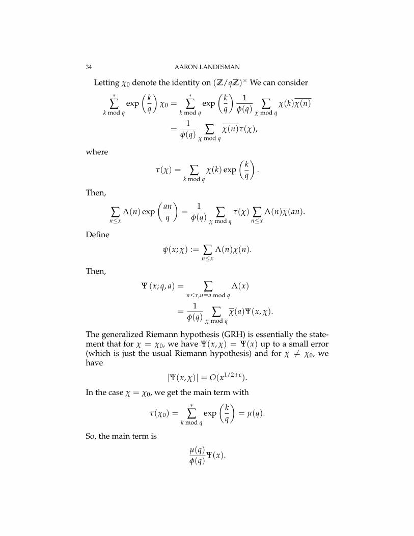
Letting χ0 denote the identity on (Z/qZ)× We can consider∗∑
k mod qexp
(kq
)χ0 =
∗∑
k mod qexp
(kq
)1
φ(q) ∑χ mod q
χ(k)χ(n)
=1
φ(q) ∑χ mod q
χ(n)τ(χ),
where
τ(χ) = ∑k mod q
χ(k) exp(
kq
).
Then,
∑n≤x
Λ(n) exp(
anq
)=
1φ(q) ∑
χ mod qτ(χ) ∑
n≤xΛ(n)χ(an).
Define
ψ(x; χ) := ∑n≤x
Λ(n)χ(n).
Then,
Ψ (x; q, a) = ∑n≤x,n≡a mod q
Λ(x)
=1
φ(q) ∑χ mod q
χ(a)Ψ(x, χ).
The generalized Riemann hypothesis (GRH) is essentially the state-ment that for χ = χ0, we have Ψ(x, χ) = Ψ(x) up to a small error(which is just the usual Riemann hypothesis) and for χ 6= χ0, wehave
|Ψ(x, χ)| = O(x1/2+ε).
In the case χ = χ0, we get the main term with
τ(χ0) =∗∑
k mod qexp
(kq
)= µ(q).
So, the main term is
µ(q)φ(q)
Ψ(x).
ANALYTIC NUMBER THEORY NOTES 35
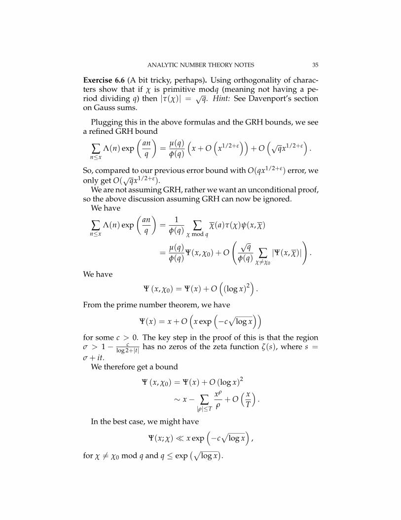
Exercise 6.6 (A bit tricky, perhaps). Using orthogonality of charac-ters show that if χ is primitive modq (meaning not having a pe-riod dividing q) then |τ(χ)| = √q. Hint: See Davenport’s sectionon Gauss sums.
Plugging this in the above formulas and the GRH bounds, we seea refined GRH bound
∑n≤x
Λ(n) exp(
anq
)=
µ(q)φ(q)
(x + O
(x1/2+ε
))+ O
(√qx1/2+ε
).
So, compared to our previous error bound with O(qx1/2+ε) error, weonly get O(
√qx1/2+ε).
We are not assuming GRH, rather we want an unconditional proof,so the above discussion assuming GRH can now be ignored.
We have
∑n≤x
Λ(n) exp(
anq
)=
1φ(q) ∑
χ mod qχ(a)τ(χ)ψ(x, χ)
=µ(q)φ(q)
Ψ(x, χ0) + O
( √q
φ(q) ∑χ 6=χ0
|Ψ(x, χ)|)
.
We have
Ψ (x, χ0) = Ψ(x) + O((log x)2
).
From the prime number theorem, we have
Ψ(x) = x + O(
x exp(−c√
log x))
for some c > 0. The key step in the proof of this is that the regionσ > 1 − c
log 2+|t| has no zeros of the zeta function ζ(s), where s =
σ + it.We therefore get a bound
Ψ (x, χ0) = Ψ(x) + O (log x)2
∼ x− ∑|ρ|≤T
xρ
ρ+ O
( xT
).
In the best case, we might have
Ψ(x; χ)� x exp(−c√
log x)
,
for χ 6= χ0 mod q and q ≤ exp(√
log x).

36 AARON LANDESMAN
The conclusion is that if
q ≤ exp(
c√
log x)
for c small, then
∑n≤x
Λ(n) exp(
anq
)=
µ(q)φ(q)
x + O(
x exp(−c√
log x))
.
In a similar way, one would like to show
ψ(x; q, a) =x
φ(q)+ O
(x exp
(−c√
log x))
.
The short version of the story is that we can basically do this, butwith one important caveat, which is called a Landau-Siegel zero.
6.4. Siegel Zeros. We want to understand Ψ(x; χ). If χ 6= χ0, wehave
Ψ(x, χ) = − ∑ρχ,|ρχ|≤T
xρχ
ρχ+ O
(x (log x)2
T
)where ρχ are the zeros of
L(s, χ) :=∞
∑n=1
χ(n)ns .
One can find proofs of all of these things in Davenport. If χ isprimitive then L(s, χ) has a functional equation of the form( q
π
)s/2Γ(
s + α
2
)L(s, χ)
where α is either 0 or 1 depending on whether χ(−1) = 1, (so α = 0)or χ(−1) = −1 (so α = 1). This yields the volume at 1− s. One cancount the number of zeros of ζ(s) or L(s, χ) up to height T, which isapproximately
T log qT2π
.
It is also useful to know the Hadamard factorization, which, onceyou know this is an order 1 function, tells you this has a factorizationin terms of its zeros. That is,
L(s, χ) =
(∏
ρ
(1− s
ρes/ρ
))eA+Bs.
So the sum of the reciprocals of the squares of the 0’s converge, butpossibly not the sum of the reciprocals of the 0’s.
ANALYTIC NUMBER THEORY NOTES 37
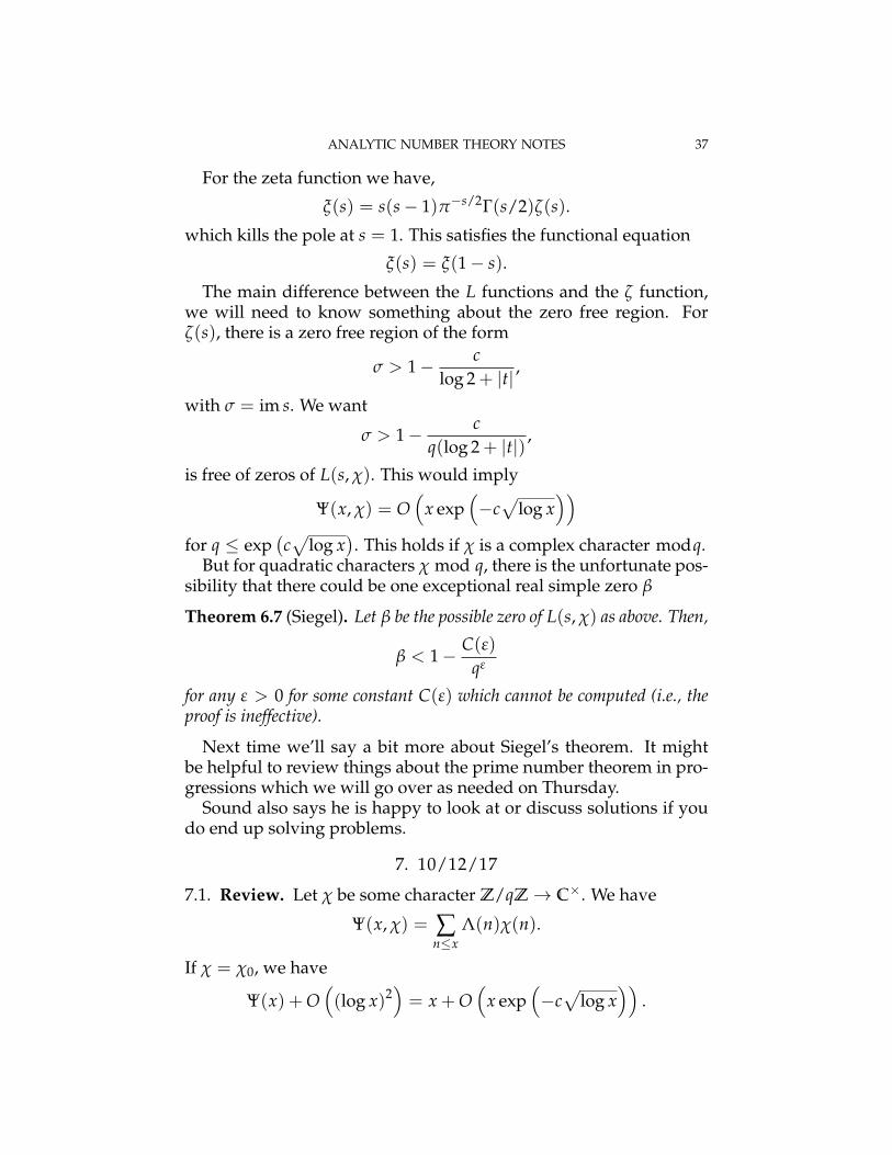
For the zeta function we have,
ξ(s) = s(s− 1)π−s/2Γ(s/2)ζ(s).
which kills the pole at s = 1. This satisfies the functional equation
ξ(s) = ξ(1− s).
The main difference between the L functions and the ζ function,we will need to know something about the zero free region. Forζ(s), there is a zero free region of the form
σ > 1− clog 2 + |t| ,
with σ = im s. We want
σ > 1− cq(log 2 + |t|) ,
is free of zeros of L(s, χ). This would imply
Ψ(x, χ) = O(
x exp(−c√
log x))
for q ≤ exp(c√
log x). This holds if χ is a complex character modq.
But for quadratic characters χ mod q, there is the unfortunate pos-sibility that there could be one exceptional real simple zero β
Theorem 6.7 (Siegel). Let β be the possible zero of L(s, χ) as above. Then,
β < 1− C(ε)qε
for any ε > 0 for some constant C(ε) which cannot be computed (i.e., theproof is ineffective).
Next time we’ll say a bit more about Siegel’s theorem. It mightbe helpful to review things about the prime number theorem in pro-gressions which we will go over as needed on Thursday.
Sound also says he is happy to look at or discuss solutions if youdo end up solving problems.
7. 10/12/17
7.1. Review. Let χ be some character Z/qZ→ C×. We have
Ψ(x, χ) = ∑n≤x
Λ(n)χ(n).
If χ = χ0, we have
Ψ(x) + O((log x)2
)= x + O
(x exp
(−c√
log x))
.
38 AARON LANDESMAN
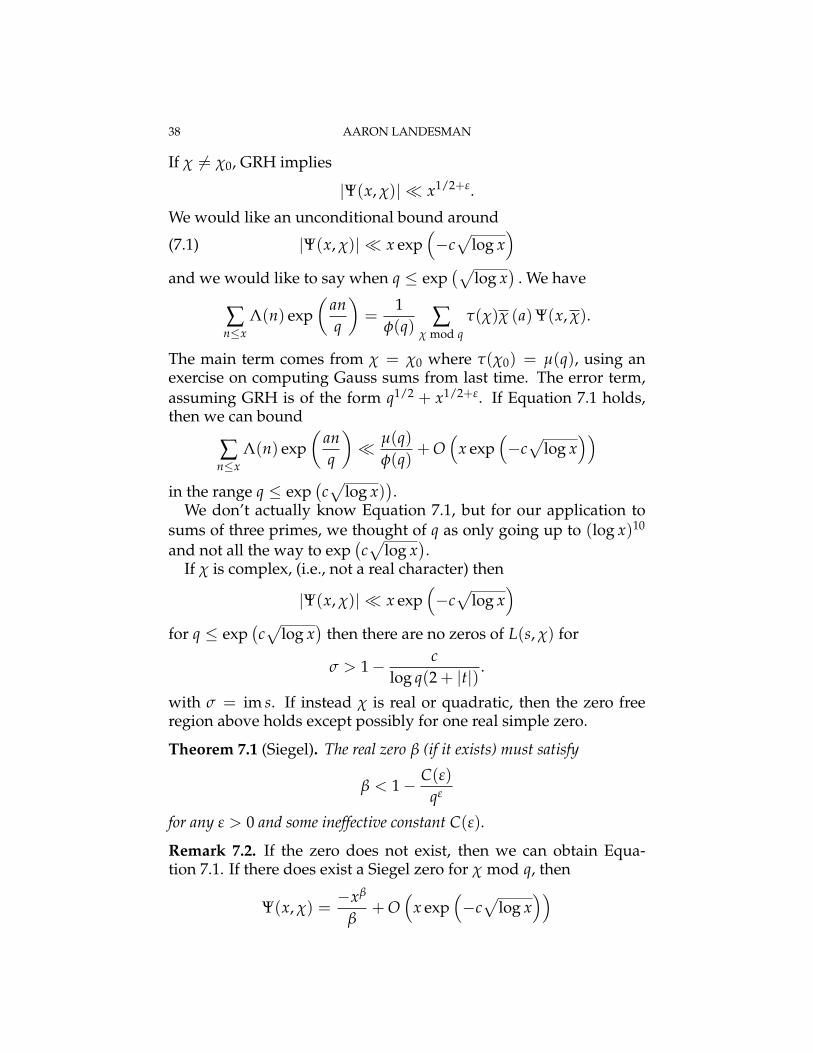
If χ 6= χ0, GRH implies
|Ψ(x, χ)| � x1/2+ε.
We would like an unconditional bound around
|Ψ(x, χ)| � x exp(−c√
log x)
(7.1)
and we would like to say when q ≤ exp(√
log x)
. We have
∑n≤x
Λ(n) exp(
anq
)=
1φ(q) ∑
χ mod qτ(χ)χ (a)Ψ(x, χ).
The main term comes from χ = χ0 where τ(χ0) = µ(q), using anexercise on computing Gauss sums from last time. The error term,assuming GRH is of the form q1/2 + x1/2+ε. If Equation 7.1 holds,then we can bound
∑n≤x
Λ(n) exp(
anq
)� µ(q)
φ(q)+ O
(x exp
(−c√
log x))
in the range q ≤ exp(c√
log x)).
We don’t actually know Equation 7.1, but for our application tosums of three primes, we thought of q as only going up to (log x)10
and not all the way to exp(c√
log x).
If χ is complex, (i.e., not a real character) then
|Ψ(x, χ)| � x exp(−c√
log x)
for q ≤ exp(c√
log x)
then there are no zeros of L(s, χ) for
σ > 1− clog q(2 + |t|) .
with σ = im s. If instead χ is real or quadratic, then the zero freeregion above holds except possibly for one real simple zero.
Theorem 7.1 (Siegel). The real zero β (if it exists) must satisfy
β < 1− C(ε)qε
for any ε > 0 and some ineffective constant C(ε).
Remark 7.2. If the zero does not exist, then we can obtain Equa-tion 7.1. If there does exist a Siegel zero for χ mod q, then
Ψ(x, χ) =−xβ
β+ O
(x exp
(−c√
log x))
ANALYTIC NUMBER THEORY NOTES 39
If q ≤ (log x)A, we can choose ε small enough, we can ensure β <
1− C√log x
, and then we can absorb the main term for Ψ(x, χ) − xβ
β
into the error term. In the presence of the Siegel zero, we can onlyget this uniform desired result for q ≤ (log x)A, but not for q ≤exp
(c√
log x). This is also ineffective.
Therefore, we obtain
∑n≤x
Λ(n) exp(
anq
)� µ(q)
φ(q)x + O
(x exp
(−c√
log x))
.
Remark 7.3. Suppose β is very close to 1. Pretend β = 1. Then thereis one character χ mod q so that Ψ(x, χ) is approximately −x.
If you think of
Ψ(x; q, a) =1
φ(q) ∑ χ(a)ψ(x, χ) =x
φ(q)− xβ
β
χ(a)φ(q)
.
and here χ is real so χ(a) = χ(a). Then, half of the progression getmost of the primes and the other half get none of them (this happensdepending on whether χ(a) = ±1).
7.2. Proving Vinogradov’s theorem using Siegel’s theorem. For themoment, we’ll assume Siegel’s theorem and finish the proof of Vino-gradov’s theorem. We’ll later come back to discuss Siegel’s theorem.
We have seen that if
q ≤ (log x)A
(A is around 10) then
∑n≤x
Λ(n) exp(
anq
)=
µ(q)φ(q)
+ O(
x exp(−c√
log x))
.
The major arcs are of the form∣∣∣∣α− aq
∣∣∣∣ ≤ 1qQ
,
with
Q =N
(log N)10
for q ≤ (log N)10. Recall we have already bounded the minor arcs,and we are now trying to bound the major arcs. Set α = a
q + β. We
40 AARON LANDESMAN
would like to understand
S(α) := ∑n≤N
Λ(n) exp(
anq
)exp (nβ) .
We can think of the the product of Λ(n) exp(
anq
)whose partial sums
we understand and exp (nβ) which doesn’t vary very much. So,
S(α) = ∑n≤N
Λ(n) exp(
anq
)exp (nβ)
=∫ N
1exp(xβ)d
(∑
n≤xΛ(n) exp
(anq
))
=µ(q)φ(q)
∫ N
1exp(xβ)dx + O
(N exp
(−c√
log N))
+ O(∫ N
1βx exp
(−c√
log x)
dx)
= O((
1 + N|β|N exp(−c√
log N)))
= O(
N exp(−c√
log x))
.
Where we used integration by parts to get the above bounds on theerror terms, and then we used that β ≤ 1
qQ , and we might have toadjust the constant c to absorb some factors of log N.
Remark 7.4. The above bound makes sense: If β is very close to aq ,
we pick up the same error term we had before. But if β is very far,then the error term should group approximately proportionally toN |β|, which indeed it does.
We now want to evaluate the major arc contribution∫M
S(α)3e (−Nα) dα.
We are hoping this is of size N2 · C with C some constant we canevaluate.
Indeed,∫M
S(α)3e (−Nα) dα = ∑q≤(log N)10
∗∑
a mod q
∫ 1/qQ
−1/qQS(
aq+ β
)3
exp(−N
(aq+ β
))dβ.
We know
S(
aq+ β
)3
=µ(q)φ(q)3
(∫ N
0exp (xβ) dx
)+ O
(N3 exp−c
√log N
)
ANALYTIC NUMBER THEORY NOTES 41
The error term in the integral over the major arcs is then
O
∑q≤(log N)10
N3 exp(−c√
log N) 1
Q
= O(
N2 exp(−c√
log N))
.
So the error terms are under control. We now want to understand themain term. The main term is almost independent of a except for thefactor exp
(−N
(aq + β
)). We want to understand the main term of∫
MS(α)3e (−Nα) dα.
which is
∑q≤(log N)10
∗∑
a mod q
∫ 1/qQ
−1/qQ
µ(q)φ(q)3
(∫ N
0exp (xβ) dx
)exp
(−N
(aq+ β
))dβ.
Recall the Ramanujan sum
cq(N) := ∑(a,q)=1
exp(
aNq
).
The main term is then
∑q≤(log N)10
µ(q)φ(q)3 cq(N)
∫ 1/qQ
−1/qQ
(∫ N
0exp (xβ) dx
)3
e (−Nβ) dβ.
We can now replace∫ N
0exp(xβ)dx = N
∫ 1
0exp (Nxβ) dx.
This yields∫ 1/qQ
−1/qQ
(∫ N
0exp (xβ) dx
)3
e (−Nβ) dβ
= N)∫ 1/qQ
−1/qQN3(∫ 1
0exp (Nxβ) dx
)3
e (−Nβ) dβ
= N2∫ N/qQ
−N/qQ
(∫ 1
0exp (Nxβ) dx
)3
e (β) dβ
= N2∫ ∞
−∞
(∫ 1
0exp (Nxβ) dx
)3
e (β) dβ + O(
q2Q2
N2
)
42 AARON LANDESMAN
where the last step uses that the tail is∫|β|>N/qQ
O(
dβ
β3
)= O
(q2Q2
N2
).
This integral above is called the singular integral. Plugging in thisremainder term, we get that the error contribution is
O
Q2 ∑q≤(log N)10
1φ(q)3 φ(q)q2
= O(
Q2 (log N)10)
= O
(N2
(log N)10
).
So, we can replace our integral from −N/qQ to N/qQ by an inte-gral going off to infinity. This integral is essentially computing thenumber of ways to write N as a sum of three numbers, which is es-sentially N2/2. But, we can also compute it since this is essentially aFourier transform. That is,
N2∫ ∞
−∞
(∫ 1
0exp (Nxβ) dx
)3
e (β) dβ
is the convolution of χ[0,1] ∗ χ[0,1] ∗ χ[0,1] which has Fourier transformabove, and for this convolution we get∫
t1,t2,t3∈[0,1]δ (t1 + t2 + t3 = 1) .
Then one can use Parseval’s identity to compute the Fourier trans-form of this. Here, Parseval is counting the number of ways of writ-ing 1 as a sum of three real numbers. Before we were writing N as asum of three integers.
Now, let’s finish our calculation. We were trying to compute
∑q≤(log N)10
µ(q)φ(q)3 cq(N)
∫ 1/qQ
−1/qQ
(∫ N
0exp (xβ) dx
)3
e (−Nβ) dβ.
which is approximated, using our above discussion, by
∑q≤(log N)10
µ(q)φ(q)3 cq(N)
N2
2.
ANALYTIC NUMBER THEORY NOTES 43
This sum is called the singular sum The tail of this sum is roughly
∑q>(log N)10
O
(1
φ(q)
2)� (log N)−10 .
Therefore, the main term is of the form
N2
2
∞
∑q=1
µ(q)φ(q)3 cq(N).
Let
S (N) :=∞
∑q=1
µ(q)φ(q)3 cq(N).
We can write, using the Chinese remainder theorem so that cp1 p2(N) =cp1(N)cp2(N). So we have
S (n) = ∏p
(1− 1
(p− 1)s cp(n))
.
Then,
cp(N) =p−1
∑a=1
exp(
aNp
)
=
{−1 if p - Np− 1 if p | N
Then,
S (n) = ∏p
(1− 1
(p− 1)s cp(n))
= ∏p-N
1 +1
(p− 1)3 ·∏p|N
(1− 1
(p− 1)2
) .
Remark 7.5. We see this cancels out when N is even. When N iseven, the major arc at 0 is cancelled by the major arc at 1/2. And ingeneral, the major arc at a/q is canceled by a similar one at a/2q.
44 AARON LANDESMAN
Finally, we have∫ 1
0S(α)3e (−Nα) = ∑
n1+n2+n3=N
=N2
2S (N) + O
(N
log N
).
Because the contribution of prime squares and cubes is negligible,we get that every sufficiently large odd number is the sum of threeprimes (and in fact it is the sum of three primes in many ways),where here we are using that
S (N) ≥ c
for all N where c is some universal constant bounded below by
2 ·∏p≥3
(1− 1
(p− 1)2
).
This finishes the proof.
Remark 7.6 (Philosophy). Under suitable situation, we’d like to saywe can get an answer by counting contributions at each place andthen multiplying them together.
For example, say we’d like to count the number of ways to write2N = p1 + p2. We can try to do the same computation mod p (i.e.,the counting the number of (a, b) so that N = a + b mod p for a, brelatively prime to p, and similarly over the infinite place). We couldthen approximate
∑n1+n2=2N
Λ(n1)Λ(n2) ∼ S (N)2N,
we can then try to use the circle method to approximate∫ 1
0 S(α)2e(−2Nα)dα.But we can no longer use Parseval’s identity to bound the minor arcsbecause ∫ 1
0|S(α)|2 = ∑
n≤2NΛ(n)2 ∼ 2N log N.
Remark 7.7. At the beginning of this course, we mentioned we couldtry to count the number of ways to write N as a sum
N = xk1 + · · ·+ xk
s .

ANALYTIC NUMBER THEORY NOTES 45
Letting P = N1/k, this is approximated by the integral∫ 1
0
(∑
x≤Pexp
(nkα))s
e (−Nα) dα.
Then, we might expect
Ps/N = Ps−k.
There might then be local obstructions (e.g., squares are always 1 mod8 or 0 mod 8). Then, if S is large enough in terms of 4k, one might tryto show this can be done. Instead of trying to understand exponen-tial sums over primes, we would want to understand exponentialsums over powers. But, once S ≥ k + 1 and there are no congruenceconstructions, this sort of result should hold. For example, everylarge number should be a sum of four squares. But for three squares,there is a congruence obstruction - 7 mod 8 can never be written as asum of three squares.
It turns out you can write numbers as sums of 7 cubes. But forfifth powers, the problem turns out to be much harder.
Next time we’ll talk about effectivity and Siegel’s theorem.
8. 10/17/17
8.1. Exercises to solidify the ideas thus far. Here are two exercises,which are a bit longer and harder than usual.
Exercise 8.1 (Difficult exercise). Assume GRH. Give a bound for
∑n≤x
Λ(n) exp (nα)
for∣∣∣α− a
q
∣∣∣ ≤ 1q2 without using bilinear forms, but instead using GRH
and thinking about the prime number theorem and arithmetic pro-gressions. Hint: We discussed how to write
∑n≤x
Λ(n) exp(
naq
)∼ 1
φ(q) ∑ χ(a)τ(χ)Ψ(x, χ),
and one can input information about Ψ using GRH.One would then try to write exp
(naq
)in terms of exp (nβ) with
|β| ≤ 1qQ
and then one should try to obtain good minor arc estimates for thissummation using a “quasi-Riemann hypothesis” (i.e., assuming there
46 AARON LANDESMAN
are no zeros with σ ≥ 2/3. Unconditionally, we know informationabout primes in progressions up to some modulus. Assuming GRH,we know estimates for primes up to
√x. We can then find approxi-
mations for numbers with the denominator up to√
x. We can thenuse the prime number theorem for everything, and then we won’teven have to worry about major and minor arcs, we can hit the wholeproblem in both cases using GRH.
If one is more careful (via a result due to Hardy and Littlewood) itis enough to assume there are no zeros with σ ≥ 3/4.
Remark 8.2. On GRH, one should be able to prove
∑n≤x
Λ(n) exp (nφ)� x3/4+ε,
whereas Vinogradov’s method only gave an x4/5. To get the 3/4estimate, we would need Hardy and Littlewood’s refinement. Thisrefinement due to Hardy and Littlewood is a refinement of the Gausssum idea. One might decompose exp
(anq
)as a sum of multiplicative
characters. This incurs a loss of√
q. When one writes it as
1φ(q) ∑
χ mod qτ(χ)χ(ax),
one rewrites a number on the order of 1 as a number on the order of√q. For n ≤ x, one can write exp(nβ) in terms of integral of the form∫
|y|≤xf (y)niydy
We try to replace this additive character in x in terms of a multiplica-tive character in y. A gauss sum is then of the form
τ(χ) = ∑ exp(
nq
)χ(n).
There will then be an integral which is an analog of a Gauss sum.One then saves a factor of
√q, instead of just writing it naively by
breaking it up into progressions.
Exercise 8.3 (Difficult exercise). This exercise is to prove a theoremof Davenport. Let µ(n) be the Mobius function. Show
supα∈R
∣∣∣∣∣∑n≤xµ(n) exp (nα)
∣∣∣∣∣�Ax
(log x)A

ANALYTIC NUMBER THEORY NOTES 47
for any A > 0. You will have to figure out what happens when α ison a major or minor arc.
When α is on a minor arc, you will want to use Vinogradov’smethod and use a bilinear estimate, you will have x/
√q +√
q · x.
We use Vaughn’s identity for obtaining bilinear forms for − ζ ′
ζ (s),and we would need an analog for identifying 1
ζ (s). One would takeζ ·M for M a modifier, and play around with powers of that.
To deal with the case when α is on a major arc. This has to do withunderstanding
∑n≤x
µ(n) exp(
anq
),
for q ≤ (log x)A. One might rewrite this in terms of χ mod q. Thegoal would then be to understand
∑n≤x
µ(n)χ(n).
Many results holding for prime numbers also hold for the Mobiusfunction. For studying primes we look at something like
12πi
∫(c)
−ζ ′
ζ(s)xs ds
s,
and in this case we would be looking at1
2πi
∫(c)
1L(s, χ)
xs dss
.
For primes there is a pole at s = 1, but the pole at s = 1 becomes a 0for 1/L. So there is some cancellation.
On the major arcs, there are savings with powers of log, and onthe minor arcs there is another method using bilinear forms whichgives savings of powers of log.Exercise 8.4. Assuming GRH, show
supα∈R
∣∣∣∣∣∑n≤xµ(n) exp (nα)
∣∣∣∣∣� x3/4+ε.
Maybe 5/6 instead of 3/4 would be easier to prove. Presumably thecorrect answer is x1/2+ε. The supremum does obtain x1/2 becauseParseval tells us∫ 1
0
∣∣∣∣∣∑n≤xµ(n) exp (nα)
∣∣∣∣∣2
dα = ∑n≤x
µ(n)2.
48 AARON LANDESMAN
Remark 8.5. The minor arc technology gave use an estimate of theform
N√
q+√
qN + E
where E is some error term endemic to the method. The first twoterms are optimized when q is on the order of
√N, in which case the
first two terms give N3/4, so you cannot really do better than N3/4
with this minor arcs method. We can write exp(nα) in terms of
∑χ
∫tχ(n)nit f ,
for some function f . Here n ≤ N, α ∈ (0, 1). One than writes α = aq +
β. One does not want to use too many q’s and too many t’s. Roughlyone uses q characters χ and integrates over t which is roughly 1 +|β|x. One needs to balance what weight to put on the sum and whatweight to put on the integral. You can always choose q ≤ Q, |β| ≤
1qQ . Then, 1+ |β|N ≤ 1+ N
Q . One can choose Q ∼√
N so the integral
goes up to√
N and the sum adds over√
N terms. One looses N1/2
complexity when doing the above procedure. So it is very hard tobeat N3/4 in these major and minor arc estimates.
8.2. Zeros of ζ and L-functions. It’s good to have some intuition forwhere the 0’s come from and how you might prove these functionshave a 0-free region. We’d like to prove
ζ(1 + it) 6= 0, L(1, χ) 6= 0,
where
L (1, χ) = ∏p
(1− χ(p)
p
)−1
.
We can consider the product
ζ (1 + it) = ∏p
(1− 1
p1+it
)−1
.
How will you find t with
|ζ (1 + it)|being large or small. The small primes have a much bigger impacton this product above than the large primes. The maximum impactoccurs when the small primes are as big or small as possible.
ANALYTIC NUMBER THEORY NOTES 49
To make
|ζ (1 + it)|
large, we would like
pit ∼ 1
and to make it small we would like
pit ∼ −1
for many small primes p.
Exercise 8.6 (Simple exercise). Show that for any N, there are qua-dratic characters χ with χ(p) = 1 for all p ≤ N (and similarlyχ(p) = −1 for all p ≤ N).
Remark 8.7. Then, χ will occur to some modulus q, and q might bevery large in terms of N. If one tries to compute one of these viathe Chinese remainder theorem, one might then have the modulusexponentially large in N.
Conjecture 8.8 (Vinogradov). If χ(p) = 1 for all p ≤ N, then q > NA
for arbitrarily large A. Conversely, χ(p) = −1 for all p ≤ N thenq > NA for all large A.
Example 8.9. The least quadratic non-residue must be smaller thanqε, if Conjecture 8.8 were to hold true.
Remark 8.10. The chance that all the first N primes land heads, oneshould expect the chance is around 1/2N. So, one would expect thenumber of primes would have to be exponentially large.
Every once in a while, there can be a surprise. For example, ifD = −163. Then, (
−163p
)= −1
for p < 41. There are 12 such primes. If you think of things as cointosses, there would only be a 1/212 (since there are 12 primes up toand including 37) but 163 is substantially smaller than 212 = 4096.
L(1, χ−163) should be very small. Indeed, the Class number for-mula gives
L (1, χ−163)πh(Q(√−163
))√
163∼ π
13.
50 AARON LANDESMAN
and the class number is 1 here (and h denotes class number). Recallthat the class number formula implies that for Q
(√−D
),
L (1, χD) =πh(Q
(√−D
)√
D.
Goldfeld and Gross-Zagier’s result implies
L(
1, χ−D ≤C log D√
D
).
Siegel’s theorem implies that if χ is a quadratic character mod q, then
L(1, χ) ≥ C (ε) q−ε
for all ε > 0.
Remark 8.11. The zero free region is determined as follows. If L (β, χ) =0, then
L (1, χ) = (1− β) L′ (σ, χ)
for some β ≤ σ ≤ 1.
Exercise 8.12. Prove that if
1 ≤ σ ≤ 1− 1log q
,
then ∣∣L′ (σ, χ)∣∣ ≤ C (log q)2 .
See Davenport. Essentially you can make sense of this a little left ofthe 1 line. Then you can differentiate it and deduce this. So, youhave a bound on how close a zero can be to 1. So, if there’s a badSiegel 0 it has to be bounded away from 1.
8.3. The zero-free region of the Zeta function. We’d like to insteadlook at the completed zeta function
ξ(s) = s (s− 1)π−s/2Γ(s/2)ζ(s).
The functional equation says
ξ(s) = ξ(s− 1).
The Hadamard product formula gives
eA+Bs ∏ρ
(1− s
ρ
)es/ρ.
The trivial zeros come because the Γ(s/2) function has zeros at s =0,−2,−4, · · · .
ANALYTIC NUMBER THEORY NOTES 51
Exercise 8.13. The Riemann hypothesis is equivalent to
|ξ (σ + it)|is monotonically increasing in σ ≥ 1/2 Hint: Show that 0 by 0, theHadamard product above will be increasing.
Furthermore,
|ζ (σ + it)|is monotone increasing on σ ≥ 1.
Exercise 8.14. Let χ be an even character, i.e., χ(−1) = 1. Define
ξ (s, χ) := π−s/2Γ(s/2)L(s, χ).
Then prove
|ξ (s, χ)|is monotone increasing in σ > 1.
If ζ(1 + it) = 0, then
pit ∼ −1
for many small primes p. This implies
p2it ∼ 1
for many small primes p. This implies ζ(1 + 2it) is very big. Thisrelates to the classical inequality
ζ(σ)3 |ζ (σ + it)|4 |ζ (σ + 2it)| ≥ 1.
Then,
χ(p)pit ∼ −1
implies
χ(p)2p2it ∼ 1,
which implies
L(
1 + 2it, χ2)
is big. This would yield a contradiction unless
χ2 = χ0
and t = 0. In this case, we are considering the ζ function at 1, whichis big because it has a pole. This is the Siegel zero situation wherewe have a quadratic character and want a lower bound for L(1, χ).
52 AARON LANDESMAN
8.4. Siegel zero situation. We’ll now discuss a proof due to Gold-feld of Siegel’s theorem. We want to show that a lower bound forL(1, χ)
L(1, χ)� C(ε)q−ε
for χ a quadratic character modq. We look at the region[1− ε
10, 1]
.
Either(1) All quadratic Dirichlet L-functions have no zero in this region
We take β = 1− ε10 . We define Ψ to some character mod3.
(2) There is some quadratic character Ψ mod r for some r withL(β, Ψ) = 0 with 1 ≥ β ≥ 1− ε
10 .Consider
ζ(s)L(s, χ)L(s, Ψ)L(s, χΨ) = ∑a(n)ns .
Exercise 8.15. Check a(n) ≥ 0 for all n by just expanding the defini-tions of Dirichlet characters for the various L functions.
This function above is the Dedekind ζ function for the biquadraticextension defined by χ and Ψ. This function is always non-negativeon primes because
(1 + χ(p)) (1 + Ψ(p)) ≥ 0
and both χ, Ψ takes values ±1, 0.Then, for c > 1, consider
I :=1
2πi
∫(c)
ζ(s + β)L(s + β, χ)L(s + β, Ψ)L(s + β, χΨ)Γ(s)Xsds
where X is some large parameter that we haven’t yet defined, whichis roughly (qr)10.
Exercise 8.16. Show that1
2πi
∫(c)
XsΓ(s)ds = e−1/x.
Look at the 0’s of Γ, compute the residues, and you will see the Taylorexpansion for e−1/x.
ANALYTIC NUMBER THEORY NOTES 53
Here we have nice absolutely convergent integrals. But insteadof picking up the characteristic function, we pick up a “smoothed”version of the characteristic function.
Then, we have
I =∞
∑n=1
a(n)nβ
e−n/x.
where we are plugging in
∑a(n)nβ
and (X/n)s We have Then, we have
I =∞
∑n=1
a(n)nβ
e−n/x ≥ e−1/x ≥ 1/2.
Dirichlet L-functions are entire. The only L-function with a pole isthe Riemann zeta function. For any other character, the L functionterms cancel out every q-steps. For example, using integration byparts
L(s, χ) =∫ ∞
1−
1ys d
(∑n≤y
χ(n)
)
= s∫ ∞
1−
1ys+1
(∑n≤y
χ(n)
)dy.
Moving the line of integration to the left, we encounter poles at1− β from the ζ function, there are poles from the Γ function. Wetake Re s = −β + 1/2, so this is negative, but not as negative as −1.We encounter poles at
s = 1− β, s = 0
coming from ζ(s + β) and Γ(s). The pole at s = 1− β has residueComputing the residue at 1− β we get
L (1, χ) L (1, Ψ) L (1, χΨ) X1−βΓ(1− β).
The residue at 0 is given as follows: near 0, we have Γ(0) ∼ 1s using
that s · Γ(s) = Γ(s + 1) and Γ(1) = 1 and is smooth.The residue at 0 is
ζ(β)L(β, χ)L(β, Ψ)L(β, χΨ) ≤ 0.
54 AARON LANDESMAN
Indeed, if all Dirichlet functions have no 0’s, L(β, χ) is positive andL(β, Ψ), L(β, χΨ) is positive, and ζ(β) is negative. In the second caseL(β, Ψ) = 0.
We then have a lower bound for the residue at 1− β. This is whatwe want, because we want a lower bound for L(1, χ). We would bedone if we had upper bounds for the latter Dirichlet L functions. Wecan just replace using integration by parts
L(s, χ) =∫ ∞
1−
1ys d
(∑n≤y
χ(n)
)
= s∫ ∞
1−
1ys+1
(∑n≤y
χ(n)
)dy.
as above.
Exercise 8.17. Indeed show that for χ a character modq, show
|L (1, χ) | � log q.
for X a large power of qr (using Re(s) = −β + 1/2).
Therefore, we would conclude a bound of the form
L (1, χ)� (qr)−ε .
We could get an effective bound, but we don’t know what r is. Incase 1, r = 3, so things would be fine. But, if there is some violationto the Riemann hypothesis, then r depends on what the violation tothe Riemann hypothesis is. So this r is the source of the ineffectivityin Siegel’s theorem.
Next time, we’ll discuss effectivity of the 3-prime theorem. Thenwe’ll move on to discussing a theorem of Maynard:
Theorem 8.18. There are infinitely many primes with no 7 in their decimalexpansion.
9. 10/24/17
9.1. Quick recap of the proof of Siegel’s theorem. Recall that lasttime we proved Siegel’s theorem:
Theorem 9.1 (Siegel). We have
L(1, χ) >C(ε)
qε
(with C(ε) ineffective).
ANALYTIC NUMBER THEORY NOTES 55
The idea of the proof was to construct an auxiliary character Ψ modr. There were two cases. In the first case, all characters have no ze-ros [1− ε/10, 1] and we took ψ mod r =
(13
)In the second case we
assume there exists some r with a zero β ≥ 1− ε10 . The idea was to
consider1
2πi
∫(c)
ζ(s + β)L(s + β, χ)L(s + β, Ψ)L(s + β, χΨ)XsΓ(s)ds = ∑a(n)e−n/x
nβ≥ e−1/x
We then move the line of integration to Re(s) = 1/2− β. This has apole at 1− β. We obtain
L(1, χ)L(1, Ψ)L(1, χΨ)X1−βΓ(1− β).
Then, at s = 0, we have
ζ(β)L(β, χ)L(β, Ψ)L(β, χΨ) ≤ 0.
At the end of last time, we claimed
Lemma 9.2. The integral on 12 − β is negligible. That is,
12πi
∫( 1
2−β)ζ(s + β)L(s + β, χ)L(s + β, Ψ)L(s + β, χΨ)XsΓ(s)ds� 1
for appropriate values of x (we will take (qr)20).
Proof. Indeed,1
2πi
∫( 1
2−β)ζ(s + β)L(s + β, χ)L(s + β, Ψ)L(s + β, χΨ)XsΓ(s)ds
� x1/2−β∫ ∞
−∞e−|t|
∣∣∣∣ζ(12+ it)L(
12+ it, χ)L(
12+ it, Ψ)L(
12+ it, χΨ)
∣∣∣∣ dt
We want some kind of polynomial bound to show this integral isnegligible. We have
ξ(s) = s (s− 1)π−s/2Γ(s/2)ζ(s)
is entire of order 1 (meaning it doesn’t grow more than exponen-tially). We want to use the maximum modulus principal in a com-plex strip with real part between −1 and 2. It’s easy to bound ξbecause ζ is a bounded function on Re(s) = 2. Similarly, we can un-derstand asymptotics of the other terms. By the functional equation,we then also understand the value at Re(s) = −1. So, by this variantof the maximum modulus principal, we can bound |ξ (1/2 + it)| by,essentially, |ξ(2 + it)|. This cannot literally be true because it wouldimply the Riemann hypothesis, but if we restrict to a rectangular re-gion, bounding things from above and below, we will have good
56 AARON LANDESMAN
enough bounds. But, in any case, after making this precise, we canbound Γ by a sterling approximation, and then bound
|ζ (1/2 + it)| � (1 + |t|) .
Remark 9.3. If we instead carry this out between −ε and 1 + ε, onecan obtain the convexity bound
|ζ(1/2 + it)| � (1 + |t|)1/4+ε .
The Lindelof hypothesis says we can replace 1/4 + ε by any positiveexponent.
Altogether, we can bound
12πi
∫( 1
2−β)ζ(s + β)L(s + β, χ)L(s + β, Ψ)L(s + β, χΨ)XsΓ(s)ds
� x1/2−β∫ ∞
−∞e−|t|
∣∣∣∣ζ(12+ it)L(
12+ it, χ)L(
12+ it, Ψ)L(
12+ it, χΨ)
∣∣∣∣ dt
� x1/2−β∫ ∞
−∞e−|t| ((1 + |t|) qr)4 dt
� (qr)4 x−.4.
Now, choose x = qr20 so that (qr)4 x−.4 � 1.�
Using the above bound from the lemma, together with
12πi
∫(c)
ζ(s + β)L(s + β, χ)L(s + β, Ψ)L(s + β, χΨ)XsΓ(s)ds = ∑a(n)e−n/x
nβ≥ e−1/x
(with the last term bounded by .9) we get
L (1, χ) L (1, Ψ) L (1, χΨ) ≥ 13
xβ−1
Γ(1− β)
≥ 15(1− β) x−ε/10
= (1− β) /5 (qr)−2ε .
Then, note
L(1, χ) ≤ c log r,
L(1, χΨ) ≤ c log qr.
ANALYTIC NUMBER THEORY NOTES 57
So, one obtains
L (1, χ) ≥ C (1− β) (qr)−3ε .
The constant C is calculatable, but the reason for the ineffectivity isthat we do not know what r and β are.
Remark 9.4. One can effectively prove
L (1, χ) ≥ C√
q,
so β must be at least 1√r away from 1, or something like that. So really
the constant above only depends on r, since we can get a bound onβ from that.
9.2. Effectivity of ternary Goldbach. Returning to ternary Goldbach,we considered
∑n≤N
Λ(n) exp(
anq
).
Using q ≤ (log N)10, we found
∑n≤N
Λ(n)χ(n),
is bounded by something like −Nβ
β for β > 1− c√q . Then,
Nβ ≤ N1−c/√
q
is small compared to N only when q ≤ (log N)1.99 . But, we wantedq to go up to (log N)10 rather than (log N)2. So, we will have to useSiegel’s theorem in some range. Even though Siegel’s theorem is noteffective, we can use that Siegel zeros are rare to still get effectivityof ternary Goldbach.
Lemma 9.5. There cannot exist two primitive quadratic characters
χ1(modq1), χ2(modq2)
with Q ≤ q1, q2 ≤ Q100 and both L functions having a 0 at least 1− 10−10
log Q .
Proof. Suppose we have two such characters χ1, χ2. We’ll now playthese two characters against each other. Consider
ζ(s)L(s, χ1)L(s, χ2)L(s, χ1χ2).
This is the Dedekind zeta function of a biquadratic field, so its Dirich-let coefficients are all positive.
58 AARON LANDESMAN
Instead, consider
ξ(s)ξ(s, χ1)ξ(s, χ2)ξ(s, χ1χ2).
Consider its logarithmic derivative and evaluate at some real num-ber σ > 1. We have
ξ ′
ξ(σ) +
ξ ′
ξ(σ, χ1) +
ξ ′
ξ(σ, χ2) +
ξ ′
ξ(σ, χ1χ2)
Using the Hadamard product formula we have
ξ(s) = eA+Bs ∏ρ
(1− s
ρ
)es/ρ
then
ξ ′
ξ(s) = ∑
ρ
1s− ρ
.
Then,
Re1
s− ρ=
σ− β
|s− ρ|2.
with s = σ + it, ρ = β + iγ. On the one hand, the expression
ξ ′
ξ(σ) +
ξ ′
ξ(σ, χ1) +
ξ ′
ξ(σ, χ2) +
ξ ′
ξ(σ, χ1χ2)
is always positive. On the other hand, if we have two real zeros, wewould obtain
ξ ′
ξ(σ) +
ξ ′
ξ(σ, χ1) +
ξ ′
ξ(σ, χ2) +
ξ ′
ξ(σ, χ1χ2) ≥
1σ− β1
+1
σ− β2.
We also know
ξ(σ) = σ (σ− 1)π−σ/2Γ(σ/2)ζ(σ),
and with α equal to either 0 or 1,
ξ(σ, χ1) =(q1
π
)σ/2Γ(σ + α/2)L(σ, χ1).
ANALYTIC NUMBER THEORY NOTES 59
We get similar expressions for the other two ξ functions. Then, weobtain
ξ ′
ξ(σ) +
ξ ′
ξ(σ, χ1) +
ξ ′
ξ(σ, χ2) +
ξ ′
ξ(σ, χ1χ2)
11− σ
+12
log q1 +12
log q2 +12
log q1q2 + O(1)
+ζ ′
ζ(σ) +
L′
L(σ, χ1) +
L′
L(σ, χ2) +
L′
L(σ, χ1χ2).
We then obtain
ζ ′
ζ(σ) +
L′
L(σ, χ1) +
L′
L(σ, χ2) +
L′
L(σ, χ1χ2).
is approximated by
−∑Λ(n)
nr (1 + χ1(n) + χ2(n) + χ1χ2(n)) ,
which has all Dirichlet coefficients negative. Therefore, we have
ξ ′
ξ(σ) +
ξ ′
ξ(σ, χ1) +
ξ ′
ξ(σ, χ2) +
ξ ′
ξ(σ, χ1χ2)
11− σ
+12
log q1 +12
log q2 +12
log q1q2 + O(1)
+ζ ′
ζ(σ) +
L′
L(σ, χ1) +
L′
L(σ, χ2) +
L′
L(σ, χ1χ2)
≤ 1σ− 1
+ log q1q2 + O(1).
If β1, β2 were close to 1, we have a lower bound by something closeto 2/1− σ.
Exercise 9.6. If q1, q2 are comparable to each other, say q1 ≤ q1002 , q2 <
q1001 , then we can’t have both a lower bound by 1
σ−β1+ 1
σ−β2and an
upper bound by
1θ − 1
+ log(q1q2) + O(1)
Here, we are choosing σ to be around 1 + 10−6
log q1q2.
�
60 AARON LANDESMAN
9.3. Discriminants of number fields. Let K be a number field overQ. Then, some prime must be ramified in K because the discriminantis more than 1. In general, if K has degree n over Q, what can we sayabout dK := disc K.
Question 9.7 (Open question). Take f ∈ Z[x] of degree n irreducible.How does disc( f ) grow?
Theorem 9.8 (Minkowski, Stark-Odlyzko). The discriminant of a num-ber field K is bounded below by cn with c > 1.
Remark 9.9. Minkowski got this by thinking about lattices and usingthe geometry of numbers.
One way to think of this is the following idea going back to Stark:Let r1 be the number of real embeddings, r2 be the number of com-
plex embeddings, so that r1 + 2r2 = n. Consider the Dedekind zetafunction
ξK(s) = s(s− 1)ds/2K ζK(s)
(π−s/2Γ(s/2)
)r1 ((2π)−sΓ(s)
)r2
= (· · · )∏ρK
(1− s
ρK
)(· · · )
where · · · indicate factors we must include to make the product con-verge. This will satisfy a functional equation ξK(1− s) = ξK(s), andwill have a Hadamard product, and so on. Then,
ξ ′KξK
(σ) = ∑ρK
1σ− ρK
≥ 0.
Then,
ξ ′KξK
(σ) =1σ+
1σ− 1
+12
log dK + r1
(−12
log π +12
Γ′
Γ(σ/2)
)+ r2 (· · · ) +
ζ ′KζK
(σ).
Using that the last term ζ ′KζK(σ) is negative, and the whole sum is pos-
itive, choosing σ near 1 optimally and knowledge of Γ′Γ (1/2) and
Γ′Γ (1) gives a lower bound for the discriminant. One must choose anappropriate value of σ, Sound suggests something like σ = 1 + c
n .So, if you have a field with small discriminant, this also means
there are not many primes of small norm. The zeros of such an Lfunction are then also nicely behaved.
Exercise 9.10. Work out the details in the above remark.
ANALYTIC NUMBER THEORY NOTES 61
There is a nice survey by Odlyzko (if one searches “discriminantsOdlyzko“) and also an article by Serre on “Minorations of discrimi-nants” (in French).
Remark 9.11. The ring of integers in a number field may not bemonogenic, so the discriminant of a polynomial may be much largerthan the discriminant of a number field. We don’t have a good lowerbound on the discriminant of a polynomial.
Suppose
(log N)1.9 q ≤ (log N)10 .
suppose there is some χ mod q0 with a Siegel zero at β0. All we haveto worry about are α = a
q + β with q0 | q. We have an expression ofthe form
∑n≤N
Λ(n) exp(
anq
)=
Nµ(q)φ(q)
+ (· · · ) + τ(χ)
φ(q)χ(a)Ψ(N, χ).
The last Ψ(N, χ) is bounded by something like Nβ0/β0. So, theabove is approximated by
Nµ(q)φ(q)
+τ(χ)
φ(q)χ(a)
Nβ0
β0
and then we can then approximate these things by major and minorarcs.
We then have to change whatever main term we had before withthis new main term coming from
τ(χ)
φ(q)χ(a)
Nβ0
β0
That is, we have∫M
S(α)3 exp (−Nα) dα = ∑q≤(log N)10,q0|q
∫|β|≤ 1
S(
aq+ β
)3
exp(−N
(aq+ β
))dβ.
Then, to find the contribution of the cube of this main term, we find∗∑
a mod q
τ(χ)3
φ(q)3 χ(a)N3β0
β30
exp(−aN
q
)From χ(a) exp
(−aN
q
)we get another Gauss sum so
∗∑
a mod q
τ(χ)3
φ(q)3 χ(a)N3β0
β30
exp(−aN
q
)∼ τ(χ)4
φ(q)3N3β0−1
β30
.

62 AARON LANDESMAN
where the −1 in 3β0 − 1 is coming from the integral. Then, τ(χ) isbounded by
√q. So, the above is bounded by
q2
q3N3β0−1
β30
.
So, in conclusion, we get a bound like
∑q≤(log N)10,q0|q
N2
q� N2q0 log log N.
for q0 > (log N)1.9. Therefore, the proof is effective.
10. 10/26/17
Remark 10.1. Goldfeld Gross Zagier says
L (1, χ) ≥ c log |D|√|D|
for imaginary quadratic fields. Then, effectively, h(−D) > c log |D|.
Remark 10.2 (Euler’s idoneal numbers). Consider Q(√−D
). Can it
be that all p ≤√|D| are either ramified or inert?
Gauss’ genus theorem tells us
h (−D) ≥ 2 part of the class group = 2# primes |D = d (|D|) .
The divisor function grows as O(|D|ε). The problem is to find alldiscriminants −D < 0 where
cl(
Q(√−D
))= (Z/2Z)r .
Remark 10.3. There is work of Biro on class numbers of fields of theform Q
(√n2 + 4
).
10.1. Primes with missing digits. In general it is quite hard to an-swer questions of the form:
(1) If p is a prime, is p + 2 a primes?(2) If n is even, when is n2 + 1 prime?
Here are some theorems coming out of sieve methods.
Theorem 10.4 (Piatetski-Shapiro, 1950s). If 1 < α < 1.1, then there areinfinitely many primes of the form
bnαc.
ANALYTIC NUMBER THEORY NOTES 63
Remark 10.5. This is quite a sparse set of numbers up to x, there areonly x1/α such numbers.
Recall from Fermat that every p ≡ 1 mod 4 can be written as asum of two squares.
Theorem 10.6 (Fouvry and Iwaniec). Infinitely often, one can write p ≡1 mod 4 as p = n2 + m2 with n a prime.
Theorem 10.7 (Friedlander and Iwaniec). For p ≡ 1 mod 4 one canwrite p = m2 + n4 for infinitely many primes.
Theorem 10.8 (Heath-Brown and Li). There are infinitely many primesp ≡ 1 mod 4 with p = m2 + q4 for q primes.
Theorem 10.9 (Heath-Brown). There are infinitely many primes of theform a3 + 2b3.
Remark 10.10. This answers an old question of Hardy and Little-wood asking if there are infinitely many primes which are sums ofthree cubes.
Friedlander and Iwaniec only involves pairs m, n over sets of sizex3/4 = x1/2 · x1/4 and in Heath-Brown’s result, this only involves aset of size x2/3 up to some x.
Question 10.11. Are there infinitely many primes p = a2 + b3?
Remark 10.12. This is analogous to the question of whether there areinfinitely many elliptic curves with prime discriminant or conductor(since the discriminant of an elliptic curve in short Weierstrass formis something like 4a3 + 27b2).
The main result we’ll spend the next few lectures proving is of asimilar flavor.
Theorem 10.13 (Maynard). If q is a sufficiently large base (e.g. q = 107),write n = ∑k
j=0 njqj with 0 ≤ nj ≤ q− 1 as a base q expansion. Select aforbidden digit 0 ≤ a0 ≤ q− 1 Let
A := {n ∈N : n does not have the digit a0 base q } .
Then,
#{
n < qk : n ∈ A}= (q− 1)k
=(
qk)log(q−1)/ log q
.
64 AARON LANDESMAN
Then,
∑n<qk
n∈A
Λ(n) ∼ κa0(q) (q− 1)k .
for κa0(q) an explicit positive constant
Remark 10.14. There is also a more involved version where one ob-tains a lower bound of the form� (q− 1)k for q = 10.
One can also find elements of A that are, say, squares.
Theorem 10.15 (Mauduit and Rivat). Write primes in binary p = ∑ aj2j.Count s(p) := ∑j aj. Then, s(p) is equally likely to be 0 or 1 mod 2.
More generally, this can be done with any base replacing 2, withobvious exceptions.
There is also the following cute result: One might ask if one canfind Fermat primes, with two 1’s in the binary expansion and allother digits 0. This might be a hard problem because the set is quitesparse, but, one can try to further ask if there are infinitely manyprimes with k 1’s. One might try an easier problem asking if theresimply exist primes with exactly k 1’s in their binary expansion. Thefollowing theorem shows the answer is yes.
Theorem 10.16 (Drmota, Mauduit, and Rivat). Let K be an integer andlet k be on the scale of K/2 (say k− K/2 = O(
√k)). Then,{
p < 2K : p prime , there are k digits equal to 1}
has an asymptotic formula, with about 1/k of the numbers in this set prime.
Remark 10.17. One would expect about ( KK/2) ∼
2K√
K
Theorem 10.18 (Bourgain). There are primes p ≤ 2k for which you canspecify any αK of the binary digits, for some fixed α > 0, where the lastdigit must be 1 (so that the number is not even).
10.2. Beginning the proof of Maynard’s theorem. We now turn toproving Maynard’s theorem on primes without a specified digit. Re-call we have fixed a base q, an integer k, and defined A as the set ofprimes up to qk without a digit a0.
ANALYTIC NUMBER THEORY NOTES 65
We are trying to count
∑n<qk
n∈A
Λ(n) = ∑n<qk
Λ(n)1A(n).
=∫ 1
0S(α)A (−α)dα,
where
S(α) = ∑n<qk
Λ(n) exp(nα)
and
A (−α) = ∑n<qk
n∈A
exp (−nα) .
In our situation, we can understand the Fourier transform of Aso well that we can actually understand its L1 norm. It is binary be-cause we are intersecting two sets here: primes and integers withouta specified digit.
We could still use the circle method here, but it is a little easier toapply the circle method in a discrete setting.
10.3. The circle method in a discrete setting. Consider
1qk
qk−1
∑a=0
S(
aqk
)A
(−aqk
)= ∑
m,n<qk
m≡n mod qk
Λ(m)1A(n)
= ∑n≤qk
Λ(n)1A(n).
The last equality holds because m, n < qk. For the penultimate one,writing
S(
aqk
)= ∑
mΛ(m) exp
(amqk
)and
A
(−aqk
)= ∑
n1A(n) exp
(−na
qk
),
and the only terms that survive are m ≡ n mod qk. This is an excel-lent approximation to the integral from the circle method.
Exercise 10.19. Verify the above equalities.
66 AARON LANDESMAN
We now separate terms into major and minor arcs, as in the circlemethod.
We now write
aqk =
`
d+ β
with d ≤ qk/2 and |β| ≤ 1dqk/2 .
We try to approximate a/qk using rational numbers with denomi-nator at most qk/2. By Dirichlet’s theorem, we can always write num-bers in this form.
We write A as some large positive number. The major arcs arethose values of a with
d ≤(
log qk)A
, |β| ≤ (log qk)A
qk .
The minor arcs are the remaining values of a. The major arcs aredistinct because the denominators are small and we are taking smallintervals around each rational number.
We’ll first deal with the major arcs. The harder part will come laterwhen we deal with the minor arcs.
10.4. The major arc contribution. There are two cases:
(1) The denominator d is a small power of q(2) The denominator d is not a small power of q.
The main terms will come from the first case. Consider the sumS(α) on the major arcs of the first case, so
α =`
d+
bqk
with d a power of q. b is small (at most d) because β is bounded.Consider
S (`/d) = ∑n<qk
Λ(n) exp(`nd
)
=µ(d)φ(d)
qk + O
(qk(
log qk)4A
)where we have proved asymptotic formulas for this in certain rangesusing Siegel’s theorem.
ANALYTIC NUMBER THEORY NOTES 67
Then,
S(`
d+
bqk
)=
µ(d)φ(s)
∑n<qk
exp(
nbqk
)+ O
(qk
(log k)3A
).
If b 6= 0, the main term vanishes and S(
aqk
)= O
(qk
(log qk)3A
). So,
we will only have to worry about the terms d = 1 or d = q.Let’s now sum all these major arcs. The contribution from the error
terms of case 1 is
1qk + O
(1qk
qk(log qk
)A (q− 1)k
)
using that |A (α)| ≤ (q− 1)k. We have main terms
1qk qk (q− 1)k
if d = 1 and b = 0
1qk ∑
1≤`≤q−1d=qb=0
A
(−`q
(−1
q− 1qk))
.
Now we have to think a bit about the Fourier transform. We have
A (α) = ∑0≤n0,n1,...,nk−1≤q−1
nj 6=a0
exp
(∑
jnjqjα
)
=k−1
∏j=0
∑nj 6=a0
exp(
njqjα) .
Then, splitting contributions from j = 1, . . . , k− 1 and j = 0, we get
A
(−`q
)= (q− 1)k−1
(q−1
∑n0=0
e(−n0`
q
)− exp
(−a0`
q
))
= − exp(−a0`
q
)(q− 1)k−1
68 AARON LANDESMAN
Adding all these main terms together we get
1qk qk (q− 1)k +
1qk ∑
1≤`≤q−1A
(−`q
)(−1
q− 1qk)+
(q− 1)k−1
(q− 1)
(q−1
∑`=1
exp(−a0`
q
))
=
(q− 1)k qq−1 if a0 = 0
(q− 1)k(
1− 1(q−1)2
)if a0 6= 0
11. 10/31/17
11.1. review. Let q be a large but fixed base and let A be the set ofnumbers missing a0 ∈ [0, q− 1].
Goal 11.1. Count
∑n<qk
n∈A
Λ(n)
and show it is asymptotically ca0(q) (q− 1)k for some constant ca0(q) >0.
Let
A (α)Ak (α) := ∑n<qk
1A (n)e (nα) ,
with
S (α) = ∑n≤qk
Λ(n)e (nα) .
Our goal was to compute the discrete Fourier transform
1qk ∑
a mod qk
S(
aqk
)A
(−aqk
)=∫ 1
0S(α)A (−α)dα.
We can approximate ∣∣∣∣ aqk −
`
d
∣∣∣∣ < 1dqk/2
with d ≤ qk/2. Last time, we were trying to work out the major arccontributions over intervals with d ≤
(log qk)A
and∣∣∣∣ aqk −
`
d
∣∣∣∣ ≤(log qk)A
qk .

ANALYTIC NUMBER THEORY NOTES 69
Last time we computed the major arc contribution in the case d wasa power of q less than
(log qk)A
where we got
ca0(q) (q− 1)k =
{ qq−1 if a0 = 0 mod q1− 1
(q−1)2 if a0 6= 0.
11.2. Remaining major arcs. We next deal with the remaining majorarcs. Namely, we show those centered at `
d for d not a power of q arenegligible. We’ll put a trivial bound on S and the cancellation willcome form A (α).
We know
|S(α)| ≤ qk (1 + o(1))
trivially. We now look for cancellation in
A
(aqk
)= A
(`
d+ c)
for c at most (log qk)
A
qk , as we are on a major arc.We have
Ak(α) =k−1
∏j=0
q−1
∑nj=0,nj 6=a0
e(
njqjα) .
A crude L∞ bound will in fact work for us, as we now explain.We can bound∣∣∣∣∣∣ ∑
nj 6=a0
e(njθ)∣∣∣∣∣∣ ≤ (q− 3) + |e(nθ) + e ((n + 1)θ)|
≤ (q− 3) + 2 |cos(πθ)|= (q− 1)− 2 (1− | cos πθ|)
≤ (q− 1) exp(−cq ||θ||2
).
for some small cq > 0, where
||x|| = minn∈Z|x− n|.
Then,
|Ak(α)| ≤ (q− 1)k exp
(−cq
k−1
∑j=0
∣∣∣∣∣∣qjα∣∣∣∣∣∣2) .
70 AARON LANDESMAN
Assuming α = `d + O
((log qk)
A
qk
), we get
|Ak(α)| ≤ (q− 1)k exp
(−cq
k−1
∑j=0
∣∣∣∣∣∣qjα∣∣∣∣∣∣2)
� (q− 1)k exp
(−cq
k/2
∑j=0
∣∣∣∣∣∣∣∣qj `
d
∣∣∣∣∣∣∣∣2)
.
Remark 11.2. Note that if ||θ|| ≤ 12q then ||qθ|| = q ||θ||.
Lemma 11.3. For k in an interval of length log dlog q + 1, we can find k0 with∣∣∣∣∣∣∣∣qk0
`
d
∣∣∣∣∣∣∣∣ ≥ 12q
.
Proof. We have ∣∣∣∣qk `
d
∣∣∣∣ ≥ 1d
and now using Remark 11.2, we see that powers of q increase, andeventually the value “wraps around 1” so we get some term whichis not too small. �
Therefore,
|Ak(α)| � (q− 1)k exp(−c1
klog k
).
Therefore, these other major arcs contribute
1qk ∑
d<(log qk)A
(`,d)=1,d not a power of q
qk (q− 1)k exp(−cqk/ log k
)� (q− 1)k
(log qk
)2Aexp
(−ck
q
log k
).
which is negligible compared to the main term computed last class.
11.3. The minor arcs. The real crux of the matter for dealing withminor arcs is that it is possible to get good bounds for the L1 normof |A (α)| . We want to bound either
∑a mod qk
∣∣∣∣Ak
(aqk
)∣∣∣∣

ANALYTIC NUMBER THEORY NOTES 71
or ∫ 1
0|Ak(α)| dα.
There will be a huge amount of cancellation here.Let’s look at
|Ak(α)| =k−1
∏j=0
∣∣∣∣∣q−1
∑n=0
e(njqjα)− e(a0qjα)
∣∣∣∣∣ .
We’ll now try to bound
q−1
∑n=0
e(njqjα)− e(a0qjα)
Let θ := njqjα. Then, we have
q−1
∑n=0
e(njqjα)− e(a0qjα) ≤ min(
q− 1, 1 +∣∣∣∣1− e(qθ)
1− e(θ)
∣∣∣∣)We have ∣∣∣∣1− e(qθ)
1− e(θ)
∣∣∣∣ ≤ 22 |sin πθ|
=1
2 ||θ|| .
Therefore,q−1
∑n=0
e(njqjα)− e(a0qjα) ≤ min(
q− 1, 1 +∣∣∣∣1− e(qθ)
1− e(θ)
∣∣∣∣) ≤ min(
q− 1, 1 +1
2 ||θ||
).
We now plug this in above for each θ = qjα. We have
|Ak(α)| ≤k−1
∏j=0
min
(q− 1, 1 +
12∣∣∣∣qjα
∣∣∣∣)
Let’s write
α =b1
q+
b2
q2 +b3
q3 + · · ·
for 0 ≤ bj ≤ q− 1. Multiplying by qjα yields
z +bj+1
q+ ε j
72 AARON LANDESMAN
with z and integer and 0 < ε j ≤ 1q . Therefore, the distance to the
nearest integer of qjα is well determined by bj+1. We have goodbounds whenever bj+1 6= 0, q− 1, while at bj+1 = 0, q− 1, we needto use the rather poor bound of q− 1.
Putting the above together, we have
|Ak(α)| ≤k−1
∏j=0
min
(q− 1, 1 +
12∣∣∣∣qjα
∣∣∣∣)
=
q− 1 if bj+1 = 0 or q− 11 + q
2bj+1if 1 ≤ bj+1 ≤ q−1
2
1 + q2(q−1−bj+1)
if q−12 ≤ bj+1 ≤ q− 2.
Plugging this in a summing over all possibilities for digits, we have
∑a mod qk
∣∣∣∣Ak
(aqk
)∣∣∣∣ = k
∏j=1
(α(q− 1) +
q−1/2
∑b=1
(2 +
qbi
))
=k
∏j=1
(3q + q log q) .
From the above, we have deduced the following lemma.
Lemma 11.4. We have
∑q mod qk
∣∣∣∣A (aqk
)∣∣∣∣ ≤ (3q + q log q)k
and ∫ 1
0|Ak(α)| dα ≤ (3 + log q)k .
So if q is large, there is a lot of cancellation, but if q is small, wewon’t get very much.
Before continuing the proof, let’s motivate this. Recall that in oursum of three primes problem, we had some bound of the form
∑n≤x
Λ(n)e(nα)�(
x4/5 + x/√
q +√
qx)
ANALYTIC NUMBER THEORY NOTES 73
Here |α− aq | =
1q2 for x.9x ≥ q > x.1. On the L1 norm in this lemma,
we’re only using a very small power of x. As long as the denom-inators are not too small or large, we are doing well on the minorarcs.
Then, we want to bound1qk ∑
a
∣∣∣Ak(a/qk)S(−a/qk)∣∣∣
where the latter is bounded by qk/(log qk)A and the former is boundedby the lemma. This will work out when d ≥ q.01k in `/d. So wewould be happy for large q.
The second idea will be used to estimate ∑Nj=1∣∣Ak(αj)
∣∣ for rela-tively few values of αj. We’ll need an additional spacing conditionthat
∣∣αi − αj∣∣ ≥ δ if j 6= i. This is natural because∣∣∣∣ `1
d1− `2
d2
∣∣∣∣ ≥ 1d1d2
.
Estimates like this are called large sieve estimates. These are usuallydone in L2, but here we’ll do an L1 estimate.
Lemma 11.5. With the spacing condition that∣∣αi − αj
∣∣ ≥ δ if j 6= i. wehave
N
∑j=1
∣∣Ak(αj)∣∣� (
1δ+ qk
)(3 + log q)k
Our hope to get a bound is something like N∫ 1
0 |A (α)| dα.
Remark 11.6 (Sobolev inequality). We have
f (t) = f (u)−∫ u
tf ′(v)dv.
Integrating both over u ∈(
t− δ2 , t + δ
2
), we have
δ | f (t)| ≤∫ t+δ/2
t−δ/2| f (u)|+
∫ t+δ/2
t−δ/2δ| f ′(v)|dv.
Then
| f (t)| � 1δ
∫ t+δ/2
t−δ/2| f (u)|du +
∫ t+δ/2
t−δ/2
∣∣ f ′(v)∣∣ dv.
Since all points αj were at least δ apart, these intervals will not over-lap when proving the lemma.
74 AARON LANDESMAN
Proof. We have the boundN
∑j=1
∣∣Ak(αj)∣∣� 1
δ
∫ 1
0|Ak(α)| dα +
∫ 1
0
∣∣A ′k (α)∣∣ dα
� 1δ(3 + log q)k +
∫ 1
0
∣∣A ′k (α)∣∣ dα
Using
A (α) = ∑n<qk
e(nα)1A(n),
we get
A ′(α)2πi ∑n<qk
ne(nα)1A(n)
Writing
n =k−1
∑j=0
njqj
we have∣∣Aj(α)∣∣� k−1
∑j=0 6=a0
∑nj
njqje(
njqjα) k−1
∏i=0,i 6=j
(∑
ni 6=a0
e(
niqiα))
� qk · Bwhere B was the bound for A (α). Then, integrating it out, we againget a bound qk (3 + log q)k. �
The idea to finish the proof is to use the above lemma’s boundwith a different k. We will continue bounding the minor arcs nexttime using our lemmas with other values of k.
12. 11/2/17
12.1. Review. Last time, we wanted to evaluate1qk ∑
a mod qk
Ak
(aqk
)S(−aqk
).
We had the major arcs which were{aq
:aq=
`
d+ η, d =
(log qk
)A, |η| ≤
(log qk)A
qk
}.
ANALYTIC NUMBER THEORY NOTES 75
We gave an asymptotic formula for these major arcs of the form
ca0(q) (q− 1)k .
This did not depend on the size of q and is true for any base at least3 or so.
It remains to deal with the minor arcs. Last time, we saw we couldestimate the L1 norm of Ak. We showed
1qk ∑
∣∣∣∣Ak
(aqk
)∣∣∣∣� (3 + log q)k
We also found ∫ 1
0|Ak(α)| dα� (3 + log q)k .
By a Sobolev type argument, we saw that if
α1, . . . , αN
are δ spaced (i.e.,∣∣αi − αj
∣∣ ≥ δ if i 6= j.Then,
N
∑j=1
∣∣Ak(αj)∣∣ ≤ (1
δ+ qk
)(3 + log q)k .
12.2. Bounding the minor arcs. Recall that by Dirichlet’s theorem,∣∣∣∣ aqk −
`
d
∣∣∣∣ ≤ 1dqk/2
using Dirichlet’s theorem with Q = qk/2, with d ≤ qk/2. We canassume d ≥
(log qk)A
as we are on the minor arcs.For now, fix a choice of B and D (where we will split d into dyadic
intervals based on D and qk|η| into dyadic intervals based on D). Wewill later range over different possibilities of D and B.
We will split this into terms with D ≤ d ≤ 2D. We won’t worryabout over-counting because we’ll ultimately estimate things by tak-ing absolute values. Write
aqk =
`
d+ η
and so that B ≤ qk|η| ≤ 2B and
qk(
η +`
d
)∈ Z.
We also need to consider the case where qk|η| ≤ 1.
76 AARON LANDESMAN
The number of choices for η with qk|η| between B and 2B is roughly2B (since η can be negative). We have D ≤ qk/2. Then qk|η| �qk/2/D. We can assume
B� qk/2/D.
Being on a minor arc means either
(1) D ≥(log qk)A
.
(2) or if D is small then B ≥(log qk)A
.So, being on a minor arc means BD is somewhat large.
Goal 12.1. We now want to understand the contribution of one ofthese dyadic blocks.
We want to understand
∑D≤d≤2D
∑(`,d)=1
∑η
qk|η|∼Bqk(η+`/d)∈Z
∣∣∣∣Ak
(`
d+ η
)∣∣∣∣ .
This is a sum containing about D2B terms. This number of terms inthe sum is then at most qk/2D � qk since B� qk/2/D.
Recall that we are trying to estimate the number of primes up to qk
not containing the digit a0. Now, our set Ak is self similar meaning
Ak
(`
d+ η
)= ∑
n0,n1,...,nk−10≤ni≤q−1
nj 6=a0
e((
n0 + n1q + · · ·+ nk−1qk−1)
α)
where α = aq = `
d + η.
Proposition 12.2. We have
∑D≤d≤2D
∑(`,d)=1
∑η
qk|η|∼Bqk(η+`/d)∈Z
∣∣∣∣Ak
(`
d+ η
)∣∣∣∣� (q− 1)k
(D2B
)αq
where
αq =log(
qq−1 (B + log q)
)log q
ANALYTIC NUMBER THEORY NOTES 77
Then,
D2αq =(
qk1)αq
=
(q
q− 1(3 + log q)k1
).
where qk1 ∼ D2, qk2 ∼ B.
Proof. We’ll now split this sum intothe first k1 digitsthe middle k− k1 − k2 digitsthe last k2 digits
with k1 − 4k2 ≤ k.The first k1 digits is dominated by
∣∣Ak1(α)∣∣. For the middle digits,
there are (q− 1)k−k1−k2 , each bounded by 1, so we get (q− 1)k−k1−k2
as a bound. For the last digits, we get
qk−k2(nk−k2 + nk−k2+1 + · · ·
)α.
Therefore, multiplying the contributions from all the digits, we get
e((
n0 + n1q + · · ·+ nk−1qk−1)
α)=∣∣Ak1(α)
∣∣ (q− 1)k−k1−k2∣∣∣Ak2
(qk−k2α
)∣∣∣ .
Remark 12.3. Thinking about what we are doing, there are D2 pointsof the form `/d and about B points η near each `/d. Given a fixed`/d, we are multiplying it by something corresponding to each ofthe B well spaced B intervals. Then, we choose qk1 on the scale of D2
and qk2 on the scale of B.
We can bound∣∣∣∣Ak
(`
d+ η
)∣∣∣∣� (q− 1)k−k1−k2
(sup|η|∼B/qk
∣∣∣∣Ak1
(`
d+ η
)∣∣∣∣) ∣∣∣∣Ak2
(1
qk2
(qk(`
d+ η
)))∣∣∣∣ .
Note that the last Ak2 term corresponds to B well spaced points mod1. That is there are B 1
qk2(since we chose qk2 ∼ B, and in fact we will
need qk2 < B).Now, we sum this over `, d, η. By a lemma from last time, fixing
`, d and summing over η, we get
∑η
∣∣∣∣Ak2
(1
qk2
(qk(`
d+ η
)))∣∣∣∣ ∼ qk2 (3 + log q)k2 .
78 AARON LANDESMAN
Then, we want to compute
(q− 1)k−k1−k2 ∑`,d,d∼D
(sup|η|∼B/qk
∣∣∣∣Ak1
(`
d+ η
)∣∣∣∣)
� (q− 1)k−k1−k2 qk1 (3 + log q)k1
using the lemma from last time again and the fact that rational num-bers with denominator on the order of D are 1
D2 spaces. �
The bound of the above proposition yields a useful bound whenD2B is small compared to qk, where this bound starts to beat the L1
bound.We want
∑d∼D
∑`
∑η,qk|η|∼B
|Ak (`/d + η) |∣∣∣∣S(−( `
d+ η
))∣∣∣∣� (q− 1)k
(D2B
)αqmax
d∼D,qk|η|∼B
∣∣∣∣S( `
d+ η
)∣∣∣∣ .
We want this to be small compared to (q− 1)k · qk. We already knowthat for these points, the size of∣∣∣∣S( `
d+ η
)∣∣∣∣Recall ∣∣∣∣S( `
d+ η
)∣∣∣∣ = | ∑n≤qk
Λ(n)e(nα)|.
Remark 12.4. Recall that from Vinogradov’s theorem, we found
∑n≤x
λ(n)e (nα)
we had an approximation of the form∣∣∣∣α− aq
∣∣∣∣ ≤ 1q2
was bounded by (x4/5 +
x√
q+√
xq)(log x)3 .
We can use the same bound here.
ANALYTIC NUMBER THEORY NOTES 79
We have d ≤ qk/2 and |η| ≤ 1dqk/2 . Therefore,∣∣∣∣S( `
d+ η
)∣∣∣∣�(
q4k/5 +qk√
D+√
qkD
)(log qk
)3.
The only worry is that if D is small then there is an issue, because1/√
D is big. In this case, we would like to look for savings in B. So,this is not quite enough when D is small.
Recall that the approximations `d to a
q are convergents of the con-tinued fractions. We have ∣∣∣∣ a
qk −`
d
∣∣∣∣ ∼ Bqk .
Perhaps this approximation is not too good. We could try taking laterapproximations of continued fractions, taking the next convergent.Choose a modulus Q and pick an approximation u
v with v ≤ Q and∣∣∣∣ aqk −
uv
∣∣∣∣ ≤ 1vQ
.
Arrange this so that 1dQ �
B10qk . That is, choose Q = 103qk
BD . Then,this u/v is not the same as `/d because it is a closer approximation.Further,
1dv≤∣∣∣∣ `d − u
v
∣∣∣∣ ≤ 1vQ
+2Bqk .
Further, 1vQ is small compared to 1
dv , and 1dv ≤ 32B
qk and we get
103qk
BD� v ≥ 1
10qk
BD.
So, in this case, we can redo our previous argument with a largerdenominator. Using the bound from before, we see∣∣∣∣s( `
d+ η
)∣∣∣∣�(
q4k/5 +qk√
BD
)(log qk
)3.
using that
qk√
BDqk/2 � q3k/4
and so we can absorb the third term into q4k/5.
80 AARON LANDESMAN
We are now basically done. We know BD is at least some powerof log qk. We want to find
1qk ∑
minor arcsAk
(aqk
)S(−aqk
)
�(
log qk)5
(q− 1)k maxD,B,DB≥(log qk)
A
((D2B)αq
qk/5 +
(D2B
)αq
√DB
)
Now, DB ≤ qk/2 and D ≤ qk/2, so we just need αq < 15 for the first
term to be sufficiently small and we need αq <14 for the second term
to be sufficiently small. We we just need to check αq <15 .
Let’s now examine this constraint. Recall
αq =log(
qq−1 (B + log q)
)log q
If q is sufficiently large, this will hold. Indeed, for q > 2 · 106 this willhold.
For example, if αq = .19, the first term is bounded by q−.01k and
the second term is bounded by (DB)−.12 ≤(log qk)−.12A
, and wecan choose A as large as we want so that this savings dominates(log qk)5
.
Exercise 12.5. Work out any changes in the case that q is composite.Hint: There is essentially no difference. We only used some sim-plifications for computing the major arcs. We divided major arcsinto cases that the denominators are powers of the modulus q. Onewould then have to work out differences when the denominator di-vides q, or something like that.
Remark 12.6. For further ideas along this line, look at Piatetski-Shapiroyielding primes of the form bnαc for α = 1.01.
13. 11/7/17
Today we’ll start talking about something new, the Bombieri-VinogradovTheorem. This tells us about the distribution of primes in arithmeticprogressions. Let Ψ(x; q, a) denote the number of primes up to xcongruent to a mod q. Let (a, q) = 1. We are looking to estimate
E (x; q, a) := Ψ (x; q, a)− xφ(q)
ANALYTIC NUMBER THEORY NOTES 81
The generalized Riemann hypothesis implies
|E (x; q, a)| � x1/2 (log x)2
which is good for q ≤ x1/2/ (log x)2.In conditionally, we’ll need to include Siegel zeros.
Theorem 13.1 (Bombieri-Vinogradov). For every A > 0 there exists aB > 0 so that
∑q≤Q
max(a,q)=1
maxy≤x|E (y; q, a)| � x
(log x)A
provided Q ≤ x1/2
(log x)B .
Remark 13.2. The generalized Riemann hypothesis yields a boundof the form Q · x1/2 (log x)2, which is essentially the same.
Remark 13.3. There is a trivial bound of the form
|E (x; q, a)| � xq
log x
so one trivially obtains the bound� x (log x)2 trivially, and Bombieri-Vinogradov lets us save arbitrary powers of log x.
Remark 13.4. The key ideas in the proof are(1) Bilinear forms and Vaughn’s identity(2) Primes in progressions and Siegel zeros(3) Large Sieve inequalities
13.1. Large Sieve for Additive characters. Suppose we have α1, . . . , αR ∈R/Z which are δ well-spaces, i.e., |αr − αs| ≥ δ for r 6= s.
Goal 13.5. Our goal is to bound
R
∑j=1
∣∣∣∣∣∑n=1Nane
(nαj)∣∣∣∣∣
2
.
for an ∈ C.
Instead of taking the sum in the above goal from n = 1 to N wecan re-parameterize the sum as
M+N
∑n=M+1
ane (nα) =N
∑n=1
aM+Ne ((M + n)α)
=N
∑n=1
aM+Ne(Mα) · e (nα)
82 AARON LANDESMAN
so this is no more general.
Remark 13.6. We can bound(∑n|an|
)2
≤ N ∑n|an|2
by Cauchy-Schwarz and we shouldn’t expect anything better thanthis.
Suppose on the other hand, that the an are “wiggling around inall directions randomly” and all have norm 1. If the an are behavingindependently for different values of n, and in this case we mightexpect some kind of square-root cancellation. That is, we might have
(∑ |an|2
)· R
Maybe in place of R, we might get 1δ because if R points were evenly
spaced, we would be using square root cancellation and averaging.
We now want to get estimates of the above form. We’ll provesomething stronger, but here’s a first pass:
Theorem 13.7. We have
R
∑j=1
∣∣∣∣∣ N
∑n=1
ane(nαj)∣∣∣∣∣
2
�((N +
1δ)
N
∑n=1|an|2
)
We give two proofs.
First Proof. The first step to prove this is a Sobolev argument. Wehave∣∣∣∣∣ N
∑n=1
ane(nαj)∣∣∣∣∣
2
� 1δ
∫ αj+δ/2
αj−δ/2
∣∣∑ ane(nα)∣∣2 dα
+∫ αj+δ/2
αj−δ/2
∣∣∣∣∣(
∑n
ane(nα)
)(∑n
nane(nα)
)∣∣∣∣∣ dα.
ANALYTIC NUMBER THEORY NOTES 83
Summing from 1 to R, we have
R
∑j=1
∣∣∣∣∣ N
∑n=1
ane(nαj)∣∣∣∣∣
2
� 1δ
∫ 1
0
∣∣∣∣∣∑nane(nα)
∣∣∣∣∣2
dα
+
∫ 1
0
∣∣∣∣∣∑nane(nα)
∣∣∣∣∣2
dα
1/2∫ 1
0
∣∣∣∣∣∑nnane(nα)
∣∣∣∣∣2
dα
1/2
� 1δ ∑
n|an|2 +
(∑n|an|2
)1/2(∑n|nan|2
)1/2
� 1δ ∑
n|an|2 +
(∑n|an|2
)1/2N
(∑n|an|2
)1/2 .
using Parseval’s identity. �
Second proof. This argument is based on duality. Say we have (am,n)M×Nan M× N matrix. From this we can consider three kinds of objects.
(1)
M
∑m=1
∣∣∣∣∣ N
∑n=1
amnyn
∣∣∣∣∣2
≤ CN
∑n=1|yn|2
(2) ∣∣∣∣∣ M
∑m=1
N
∑n=1
amnxmyn
∣∣∣∣∣C
(∑m|xm|2
)1/2(∑n|yn|2
)1/2
(3)
N
∑n=1
∣∣∣∣∣ M
∑m=1
amnxm
∣∣∣∣∣2
≤ C ∑m|xm|2 .
Exercise 13.8. Show one of the above three inequalities holds for allchoices of x, y if and only if the other two do. I.e., show the abovethree statements are equivalent.
By duality, in order to give the desired bound, it suffices to bound
N
∑n=1
∣∣∣∣∣ R
∑r=1
bre(nαr)
∣∣∣∣∣
84 AARON LANDESMAN
in terms of the L2 norm of b for all choices of b. Expanding this out,we get
N
∑n=1
∣∣∣∣∣ R
∑r=1
bre(nαr)
∣∣∣∣∣ = ∑r,s≤R
brbs
N
∑n=1
e (n (αr − αs)) .
Since αr and αs are all well spaced, the terms in the exponentialswon’t be close to integers very often.
There are two types of terms, those with r = s, in which case weget a contribution of N ∑r |br|2.
There are also the off-diagonal terms with r 6= s. Here,∣∣∣∣∣ N
∑n=1
e (nθ)
∣∣∣∣∣� 1||θ||
where ||θ|| is the integer nearest to θ. We can then estimate the sumof the off diagonal terms by
∑r 6=s
(|br|2 + |bs|2
) 1||αr − αs||
�∑r|br|2
(∑s 6=r
1||αr − αs||
)
�(
∑r|br|2
)(R
∑j=1
1jδ
)
�(
∑r|br|2
)(1δ
log R)
�(
∑r|br|2
)1δ
log1δ
.
using symmetry to bound the |br|2 + |bs|2 by (an implicit factor of 2times |br|2.
So, we have proved, in the dual form, that
N
∑n=1
∣∣∣∣∣∑rbre(nαr)
∣∣∣∣∣2
≤(
N + O(
1δ
log1δ
))∑
r|br|2 .
We now have an extra factor of log, and we will now explain howto remove this factor of log . We will set it up, but won’t really carryit out.

ANALYTIC NUMBER THEORY NOTES 85
Recall we were trying to estimate
∑n=1
∣∣∣∣∣ R
∑r=1
bre (nαr)
∣∣∣∣∣2
Say we start with the characteristic function between 1, N and takinga smoothing Φ of this characteristic function supported on a smallinterval around (1, N) and always positive. We instead try to esti-mate
∑n=1
Φ(n)
∣∣∣∣∣ R
∑r=1
bre (nαr)
∣∣∣∣∣2
One could image one might be able to smooth on an the interval(1− 1
δ, N +
1δ
)so that Φ is supported on this interval. We have
∑n=1
Φ(n)
∣∣∣∣∣ R
∑r=1
bre (nαr)
∣∣∣∣∣2
= ∑r,s
brbs ∑n
Φ(n)e (n (αr − αs))
= ∑r,s
brbs ∑k
Φ (k + αr − αs) .
using Poisson summation. The Fourier transform is large at 0 (aroundN + 2
δ ). You can get the rate of decay by integrating by parts manytimes. One can learn about the decay from the derivative of Φ.The Fourier transform is approximately supported on an interval oflength δ , apart from some small fluctuations. Since Φ(k + αr − αs)never gets within δ of an integer, it is always close to 0 when r 6= s.Therefore, including the contribution at r = s, we get the sum is wellestimated by
Φ(0)R
∑r=1|br|2
and we save the log term.
Exercise 13.9 (Involved exercise). Complete the above sketch into aproof
�
Remark 13.10. Here is a problem: Can on e choose Φ ≥ 0, Φ ≥ χ[1,N]
and Φ supported in (−δ, δ) minimizing Φ(0)?
86 AARON LANDESMAN
There is a solution discovered by Beurling and Selberg. One ob-tains something like Φ(0) ≤ N + 1
δ − 1.
We will next deduce the large sieve from the above theorem. Saywe have {
aq
: q ≤ Q, (a, q) = 1}
which is about Q2 points each 1Q2 spaced.
Q
∑q=1
∗∑
a mod q
∣∣∣∣∣ M+N
∑n=M+1
ane(
anq
)∣∣∣∣∣2
≤(
N + O(Q2)) M+N
∑n=M+1
|an|2.
Example 13.11 (Important example). Take an = 1 if n ∈ [M + 1, M + N]is prime and 0 otherwise. To examine the left hand side,
∗∑
a mod q∑
n prime ∈[M+1,M+N]
e(
anq
)= ∑
n∈[M+1,M+N],n prime
∗∑
a mod qe(
anq
)= ∑
n∈[M+1,M+N],n primeµ(q)
= µ(q) (π(M + N)− π(M))
where π(k) is the number of primes up to k. Using Cauchy-Schwarz,we get
φ(q)∗∑
a mod q
∣∣∣∣∣ ∑nprime
e(
anq
)∣∣∣∣∣2
≥ µ(q)2 (π(M + N)− π(M))2 .
Combining the above, the left hand side of the Large sieve is boundedby
Q
∑q=1
∗∑
a mod q
∣∣∣∣∣ M+N
∑n=M+1
ane(
anq
)∣∣∣∣∣2
≥ ∑q≤Q
µ(q)2
φ(q) (π(M + N)− π(M))2
and the large sieve implies
∑q≤Q
µ(q)2
φ(q) (π(M + N)− π(M))2 ≤
(N + O(Q2)
)(π (M + N)− π(M)) .
ANALYTIC NUMBER THEORY NOTES 87
This implies that the number of primes in the interval M to M + Nis bounded by (
N + O(
Q2))(
∑q≤Q
µ(q)2
φ(q)
)−1
.
If we make the Q too big, this O(Q2) term will start to dominate. So,we might want Q2 to be something like Q = N1/2−ε. The bound thenbecomes
N (1 + o(1))1
∑q≤N1/2−ε µ(q)2/φ(q).
Exercise 13.12. Show
∑n≤x
µ(n)2
φ(n)∼ log x.
Then, the number of primes between N and M+ N yields a boundof
N (1 + o(1))1
∑q≤N1/2−ε µ(q)2/φ(q)≤ 2N(1 + o(1))
log N
This yields
Theorem 13.13 (Brun-Titchmarsh theorem). We have
π(M + N)− π(M) ≤ 2 (1 + o(1)) Nlog N
.
Remark 13.14. The constants in this inequality can be made explicit.In fact, one can replace
π(M + N)− π(M) ≤ 2 (1 + o(1)) Nlog N
.
by
π(M + N)− π(M) ≤ 2Nlog N
.
without any error terms. That is, the number of primes from M toM + N is no more than twice the number of primes from 1 to N.
Remark 13.15. In fact, one might expect π(x) + π(y) ≥ π(x + y).This contradicts a conjecture of Hardy and Littlewood, so is expectedto be false.
88 AARON LANDESMAN
Exercise 13.16. Generalize the Brun-Titchmarsh theorem as follows.Use the Large Sieve appropriately to show
π (x; q, a) ≤ x (2 + o(1))φ(q) log(x/q)
.
For example if x = q1,000,000. Then, π(x; q, a) is at most 2.00001 timesthe expected number of primes. I.e.,
π (x; q, a) ≤ (2.000001)x
φ(q) log x.
This constant more than 2 is significant because of Siegel zeros. Then,
Ψ(x; q, a) =x
φ(q)− χ(a)
xβ
φ(q)β
for χ a quadratic character. If one could replace the 2 by 1.99 onewould imply there are no Siegel zeros.
Exercise 13.17 (What is large about the large sieve). For primes weused that one residue class is forbidden and so we get some im-balances. Now, more generally, suppose we have S ⊂ [1, N] with|S(mod p)| ≤ p+1
2 . Use the Large sieve to show
|S| ≤ N1/2+ε.
Here, the sieve is large because we are forbidding a large number ofresidue classes. Say here the primes p range up to p ≤
√N.
Remark 13.18. This bound is tight because if we take S to be the setof squares, we get the claimed number of residue classes.
Remark 13.19. There is a conjecture of Helfgott and Venkatesh say-ing that if one is missing half the residue classes and do have half theresidue classes, it should look like some quadratic polynomial.
14. 11/9/17
Last time we discussed the Large sieve in its additive form. Thatis, if α1, . . . , αR are δ well spaced, then
R
∑r=1
∣∣∣∣∣M+N
∑M+1
ane(nαr)
∣∣∣∣∣ ≤(
N + O(
1δ
))∑ |an|2 .
ANALYTIC NUMBER THEORY NOTES 89
One way we’ll apply this is by taking aq with (a, q) = 1, q ≤ Q, R =
Q2, δ ∼ 1Q2 and obtaining
∑q≤Q
∗∑
a mod q
∣∣∣∣∣ M+N
∑n=M+1
a(n)e(
anq
)∣∣∣∣∣2
≤(
N + O(Q2))
∑ |a(n)|2 .
14.1. A multiplicative version of the large sieve. We’ll now for-mulate the large sieve in a multiplicative form in order to proveBombieri Vinogradov. We’ll average over all characters χ mod q andsum over q ≤ Q.
∑q≤Q
∗∑
χ mod q
∣∣∣∣∣ M+N
∑n=M+1
a(n)χ(n)
∣∣∣∣∣2
≤(
N + O(Q2))
∑ |a(n)|2
Remark 14.1. Here the term of size N corresponds to a particular“bad character.” and the Q2 corresponds to the sum over the re-maining characters with square-root savings bounding by some L2
norm. We’d like to think characters of different moduli are orthog-onal to each other, but we don’t want to recount characters, so wehave the star on our sum to indicate we are summing over primitivecharacters χ (not induced by characters of smaller modulus).
In fact, we’ll obtain something slightly more precise than the above.We want to go from multiplicative characters to something involv-ing additive characters. We’ll want to pass between χ(n) and e
(nq
).
Let χ mod q be a primitive character. Let
τ(χ) = ∑a mod q
χ(a)e(
aq
)be the Gauss sum. Suppose (n, q) = 1. Then, consider
∑a mod q
χ(a)e(
anq
)= ∑
a mod qχ(a)e
(anq
)χ(n)χ(n)
= τ(χ)χ(n).
noting that χ(n)χ(n) = 1 if n is coprime to q. Then,
χ(n) =1
τ(χ) ∑a mod q
χ(a)e(
anq
).
This holds for all χ mod q so long as (n, q) = 1.
90 AARON LANDESMAN
Exercise 14.2. If χ is primitive, then in fact the above equality is truefor all n. That is, if n has factor in common with q, then the left handside is 0, and we have to check the right hand side is also zero solong as χ is primitive.
For example, consider q a prime. Then, every character except theprincipal character has right hand side evaluating to 0 when q | n.
We have
M+N
∑n=M+1
a(n)χ(n) =1
τ(χ) ∑a mod q
χ(a)M+N
∑n=M+1
a(n)e(
anq
).
Let
S(
aq
):=
M+N
∑n=M+1
a(n)e(
anq
).
We wanted to bound
∗∑
χ mod q
∣∣∑ a(n)χ(n)∣∣2 =
1q
∗∑
χ mod q
∣∣∣∣∣ ∑a mod q
χ(a)S(aq)
∣∣∣∣∣2
≤ 1q ∑
χ mod q
∣∣∣∣∣ ∑a mod q
χ(a)S(aq)
∣∣∣∣∣2
=φ(q)
q
∗∑
a mod q
∣∣∣∣S( aq
)∣∣∣∣2 .
using that |τ(χ)| = √q.So, using the above and the large sieve,
∑q≤Q
qφ(q)
∗∑
χ mod q
∣∣∣∣∣ M+N
∑n=M+1
a(n)χ(n)
∣∣∣∣∣2
≤ ∑q≤Q
∗∑
a mod q
∣∣∣∣S( aq
)∣∣∣∣2≤(
N + O(Q2)) M+N
∑n=M+1
|a(n)|2 .
Remark 14.3. The idea is that we are estimating some quantity onaverage, and one term is very bad and the rest of the terms havesquare-root cancellation.
ANALYTIC NUMBER THEORY NOTES 91
14.2. Proving Bombieri Vinogradov. Let Q =√
x(log x)B . Our goal is
to bound
∑q≤Q
max(a,q)=1
∣∣∣∣Ψ(x; q, a)− xφ(q)
∣∣∣∣� x
(log x)2 .
In our original statement, we also had a maximum over y up to x,which we will forget about, as it is not so important.
Recall
Ψ(x; q, a) =1
φ(q) ∑χ
χ(a)Ψ(x, χ)
=1
φ(q) ∑χ 6=χ0
χ(a)Ψ(x, χ)− xφ(q)
+ O
(x
φ(q) (log x)A+100
)and this error term is bounded using
∑q≤Q
1φ(q)
� log x.
Here we are using
1n≡a mod q =1
φ(q) ∑ χ(a)χ(n)
and so
Ψ(x; q, a) =1
φ(q) ∑χ
χ(a) ∑n≤x
Λ(n)χ(n).
Then, we get
max(a,q)=1
∣∣∣∣Ψ(x; q, a)− xφ(q)
∣∣∣∣ ≤ 1φ(q) ∑
χ 6=χ0
|Ψ(x, χ)|
Suppose χ mod q is induced by some primitive character χ mod q.We’ll assume q > 1 so the principal character does not show up, andthen q | q. Then,
∑q≤Q
1φ(q) ∑
χ mod q,χ 6=χ0
|Ψ(x, χ)| = ∑1<q≤Q
∗∑
χ mod q∑
q≤Q,q|q
1φ(q)
|Ψ(x, χ)| .
We have χ(n) = χ(n) if (n, q) = 1. If (n, q) > 1 bun (n, q) = 1 thenthe two could be different.
92 AARON LANDESMAN
We have the bound
|Ψ(x, χ)−Ψ (x, χ)| = ∑n≤x
(n,q)>1(n,q)=1
Λ(n)� log x# {p | q : p - q}
� (log x)2 .
Exercise 14.4. Show that we can bound
∑1<q≤Q
∗∑
χ mod q∑
q≤Q,q|q
1φ(q)
|Ψ(x, χ)| .
by
∑q<q≤Q
∗∑
χ mod q∑
q mod q,q≤Q
1φ(q)|Ψ(x, χ)|+ O
(Q (log x)3
)(14.1)
using the bound on the difference between Ψ(x, χ) and Ψ(x, χ) above,and so it suffices to bound Equation 14.1.
The point is that the difference is bounded by (log x)2 the numberof characters is φ(q) which cancels out and we get a factor of Q andthree factors of log.
Then, bound the inner most sum by
∑r≤Q/q
1φ(qr)
� 1φ(q)
log x
� 1q(log x)2 .
Warning 14.5. Now, we replace q by q to avoid writing lots of tildes.
Let’s break q ≤ Q into dyadic blocks
R ≤ q ≤ 2R
with R ≤ Q. There are on the order of log x such blocks. We canbound Equation 14.1 by
(log x)3 maxR≤Q
1R ∑
R≤q≤2R
∗∑
χ mod q|Ψ(x, χ)| .(14.2)
We now have two cases.(1) R is small so R ≤ (log x)10A.(2) R is large (here we will use the large sieve)
ANALYTIC NUMBER THEORY NOTES 93
Remark 14.6. We’d like to bound
∑q≤√
x/(log x)B
maxα|E(x; q, a)| � x
(log x)A .
Even if we are only interested in q ≥ x1/3, we still will have todeal with small moduli because of imprimitive characters. We couldavoid dealing with small moduli if we only sum over primes.
Exercise 14.7. Work out a Bombieri Vinogradov theorem in the rangex1/3 to Q =
√x
(log x)B for integers, all of whose prime factors are bigger
than x1/10.
14.3. The case R is small. Here we can use Siegel zeros and whatwe know about zero-free regions. If q ≤ (log x)10A then
|Ψ (x, χ)| � x
(log x)100A+100
using Siegel’s theorem.These easily yield a bound of Equation 14.2 by
x
(log x)10A+10 .
14.4. The case R is large. Now, let’s deal with the range
(log x)10A ≤ R ≤√
x(log x) B
.
We now use the trick of decomposing Λ(n) via Vaughan’s identity.We have
∑ Λ(n)e (nα)
which by Vaughan’s identity yields a good bound
∑m
∑n
ambne(mnα).
There is an issue that if we only wanted to estimate ∑n Λ(n)χ(n)for one character χ we could get something like ∑m,n ambnχ(m)χ(n).But, we’re only trying to average over all characters Q over rangingR. The idea is now to write down Vaughan’s identity and the use thelarge sieve.
94 AARON LANDESMAN
Recall Vaughan’s identity says that for
P(s) =≤m≤UΛ(n)
ns
M(s) = ∑n≤V
µ(n)ns
we have
−ζ ′
ζ(s) =
(−ζ ′
ζ(s)− P(s)
)(1− ζ(s)M(s)) + P(s)− ζ ′(s)M(s)− ζ(s)M(s)P(s)
with the first term on the right a type 2 sum and the latter three termsType 1 sums.
We’d now like to try to bound what all these terms give us.First, let’s consider the type 2 sum.
14.5. Bounding the type 2 sum. Recall we are trying to bound somesum of terms of the form ∑n Λ(n)χ(n).
Expanding Λ(n) using Vaughan’s identity, we get some bound ofthe form
∑R≤q≤2R
∗∑
χ mod q∑
m>U∑
n>V,mn≤xΛ(m) +
∑d|n,d>V
µ(d)
χ(m)χ(n).
But note that the term
∑d|n,d>V
µ(d)
is bounded by d(n), so we can essentially ignore this.
Exercise 14.8. Use a Perron type integral to separate the variables mand n. Then, group them into dyadic blocks with M ≤ m ≤ 2M, N ≤n ≤ 2N with the conditions M ≥ U, N ≥ V, MN � x to remove thedependence mn ≤ x.
Then, using the above, show
∑R≤q≤2R
∗∑
χ mod q∑
m>U∑
n>V,mn≤xΛ(m) +
∑d|n,d>V
µ(d)
χ(m)χ(n)
� (log x)3 ∑q∼R
∗∑
χ mod q
(∑
m∼MΛ(m)χ(m)
)(∑
n∼Na(n)χ(n)
).
ANALYTIC NUMBER THEORY NOTES 95
We now use Cauchy-Schwarz and ∑m∼M Λ(m)2 � M log M, ∑n∼N d(n)2 �N (log N)3 to obtain
(log x)3 ∑q∼R
∗∑
χ mod q
(∑
m∼MΛ(m)χ(m)
)(∑
n∼Na(n)χ(n)
)
� (log x)3
∑q
∗∑χ
∣∣∣∣∣ ∑m∼M
Λ(m)χ(m)
∣∣∣∣∣21/2∑
q
∗∑χ
∣∣∣∣∣ ∑n∼N
a(n)χ(n)
∣∣∣∣∣21/2
� (log x)3
((M + R2
)∑
m∼MΛ(m)2
)1/2((N + R2
)∑
n∼Nd(n)2
)1/2
� (log x)5{
M2 + MR2}1/2 {
N2 + NR2}1/2
� (log x)5{
MN +MN√
MR +
MN√N
R +√
MNR2}
� (log x)5{
x +xR√
U+
xR√V
+√
xR2}
.
Then, taking U = V = x1/10, we see
max(log x)10A≤R≤
√x/(log x)B
1R(log x)5
{x +
xR√U
+xR√
V+√
xR2}
� xlog x
A+ x (log x)5
(1√U
+1√V
)+√
x (log x)5 5√
x
(log x)B
For B > A + 10 or so we can bound all the terms by√
x/(log x)A.So, this completes the type 2 sum case.
It only remains to deal with the type 1 sum case. We’ll do thetrivial type 1 sum, which comes from P(s). This is
∑u≤U
Λ(n)ns .
We then have to bound
1R ∑
q∼R
∗∑
χ mod q| ∑
n≤UΛ(n)χ(n)| � UR
� U√
s.
Since U is small, around x1/10, we have bounded this sum.
96 AARON LANDESMAN
Next time we’ll deal with the other two terms. Let’s just give anidea of how to deal with one of them now. We’re trying to bound theterm corresponding to
ζ(s)M(s)P(s).
We want to bound
∑q∼R
∗∑
χ mod q∑
m≤U,n≤VΛ(m)µ(n) ∑
k≤x/mnχ(k)χ(m)χ(n).
We then have the problem of evaluating
∑k≤x/mn
χ(k)
which is certainly bounded by q, and we’d like to even improve thisa bit to
√q, plug it in, and take trivial estimates on everything.
15. 11/14/17
15.1. Brun-Titchmarsh. Recall a few classes ago, we were trying tobound π(M + N)− π(M). We wanted to bound
∗∑
a mod q∑
M+1≤p≤M+Ne(
apq
)= µ(q) (π(M + N)− π(M)) .
We used Cauchy-Schwarz to bound
µ(q)2 (π(M + N)− π(M))2 ≤(
∗∑
a mod q1
) ∑a mod q
∣∣∣∣∣ ∑M+1≤p≤r+N
e(
apq
)∣∣∣∣∣2 .
One then gets a bound to which one can now use the large sieve.
15.2. Back to Bombieri Vinogradov. Recall we have reduced to proofto bounding
(log x)3 maxR≤√
x/(log x)B
1R ∑
R≤q≤2R
∗∑
χ mod q|Ψ (x; χ)| .
We had two ranges. If R small, like R ≤ (log x)10A we could use ourbounds for |Ψ (x, χ)|. To conclude, we only needed to deal with
(log x)10A ≤ R ≤√
x
(log x)B
using Vaughan’s identity and the large sieve.
ANALYTIC NUMBER THEORY NOTES 97
Recall(−ζ ′
ζ(s)− P(s)
)(1− ζM(s)) = −ζ ′
ζ(s)− P(s) + ζ ′(s)M(s) + ζ(s)M(s)P(s).
with
P = ∑n≤U
Λ(n)ns
M = ∑n≤V
µ(n)ns
We were able to bound the type 2 sum by
� (log x)5(
xR+
x√U
+x√V
+√
xR)� x
(log x)A
We also bounded P by UR � x.6. Next, we bound the type 1 sumζMP given by
1R ∑
R≤q≤2R
∗∑
χ mod q
∣∣∣∣∣ ∑m≤U,n≤V
Λ(m)µ(n) ∑k≤x/mn
χ(kmn)
∣∣∣∣∣ .
We’ll also bound this crudely, forgetting about the sums over M andN, and get cancellation from the sum over k.
15.3. Polya Vinogradov theorem. We’ll prove the Polya Vinogradovtheorem:
Theorem 15.1 (Polya-Vinogradov Theorem). Suppose χ mod q is prim-itive. Then,
maxx
∣∣∣∣∣∑n≤xχ(n)
∣∣∣∣∣� √q log q
Remark 15.2. Assuming Polya Vinogradov, we can bound the type1 sum ζMP by
1R ∑
R≤q≤2R
∗∑
χ mod q
∣∣∣∣∣ ∑m≤U,n≤V
Λ(m)µ(n) ∑k≤x/mn
χ(kmn)
∣∣∣∣∣� 1
RR2UV
√R log R
� x1−ε.
98 AARON LANDESMAN
Exercise 15.3. Show
∑n≤x
χ(n) log n� √q (log q) (log x)
using Partial summation. Hint: Consider∫ x
1
(∑n≤t
χ(n)
)dtt
and obtain a log n from this integral.
Exercise 15.4. Bound ζ ′(s)M(s) in a similar way using the previousexercise. In fact, one can bound this term by
ζ ′(s)M(s)� 1R
R2V√
R (log R) (log x) .
It only remains to prove the Polya-Vinogradov Theorem.
Proof. The idea is to rewrite the character χ in terms of additive char-acters.
∑a mod q
χ(a)e(
anq
)= χ(n) ∑
a mod qχ(a)χ(n)e
(anq
)= τ(χ)χ(n)
This yields,
χ(n) =1
τ(χ) ∑a mod q
χ(a)e(
anq
).
therefore, we have
∑n≤x
χ(n) =1
τ(χ) ∑a mod q
χ(a) ∑n≤x
e(
anq
).
Summing
∑n≤x
e(
anq
)as a progression, we have
∑n≤x
e(
anq
)≤ min
x,1∣∣∣∣∣∣ aq
∣∣∣∣∣∣ .
ANALYTIC NUMBER THEORY NOTES 99
We also have
|τ(χ)| = O(1√
q).
We know ∑n≤x χ(n) ≤ x. Say −q/2 ≤ a ≤ q/2. Then,∣∣∣∣∣∣ a
q
∣∣∣∣∣∣ ∼ |a|q
and we use the bound x if |a| ≤ qa and the bound q/|a| if |a| > q/x.
Therefore, we obtain a bound
∑n≤x
χ(n) =1
τ(χ) ∑a mod q
χ(a) ∑n≤x
e(
anq
)� 1√
q(q log q)
=√
q log q.
�
Remark 15.5. Here is an alternate heuristic explanation of Polya-Vinogradov. We have
∑n
χ(n)Φ(n
x
)=
1τ(χ) ∑
a mod qχ(a)∑
nΦ(n
x
)e(
anq
)=
1τ(χ) ∑
a mod qχ(a)∑
kxΦ(
x(
k +aq
))=
1τ(χ) ∑
a mod qχ(a)∑
kxΦ(
x(
kq + aq
))=
1τ(χ) ∑
mχ(m)xΦ
(xmq
).
where we let m = kq + a. So the left hand side is a sum over χ ofsize x and the right hand side is a sum over χ of size q/x. This is aninvolution. This explains why Polya Vinogradov holds. If x <
√q
and we get a bound by√
q. If not, do the flip and bound the χ righthand side trivially which gives a bound x/
√q · q
x �√
q.
100 AARON LANDESMAN
Say we want to understand∣∣∣L (1
2 , χ)∣∣∣. We have
L(
12
, χ
)=
∞
∑n=1
χ(n)√n
=∫ ∞
1
1√
yd
(∑n≤y
χ(n)
)
=12
∫ ∞
1
1y3/2
(∑n≤y
χ(n)
)dy
where we can bound
∑n≤y
χ(n)min (y,√
q log q)
using Polya Vinogradov.
Exercise 15.6. Show the above is bounded by
� q1/4 log q.
The kind of argument we were discussing in Remark 15.5 yields
L(
12
, χ
)= ∑
n≤√q
χ(n)√n
+ ε(χ) ∑n≤√q
χ(n)√n
where ε(x) is a complex number of size 1.So, q1/4 log q is called the convexity bound for for
∣∣∣L (12 , χ)∣∣∣ .
The Riemann hypothesis implies the Lindelof hypothesis, whichimplies ∣∣∣∣L(1
2, χ
)∣∣∣∣� qε
for any ε > 0.In fact, we can slightly improve the above bound.
Theorem 15.7 (Burgess). We have∣∣∣∣L(12
, χ
)∣∣∣∣� q3/16+ε
for q cube free.
If χ is quadratic, there is an even better result:
ANALYTIC NUMBER THEORY NOTES 101
Theorem 15.8 (Conrey and Iwaniec). For χ quadratic,
L(
12
, χ
)� q1/6+ε
Burgess has a result saying q is cubefree if∣∣∣∣∣∑n≤xχ(n)
∣∣∣∣∣ = o(x)
if x ≥ q1/4+ε.
Exercise 15.9. If χ is quadratic modq for q a prime, then then theleast quadratic non-residue (lqnr) modq is at most q1/2 log q. Gaussshowed lqnr ≤ q1/2. A trick of Vinogradov allows you to save afactor of
√e and Polya Vinogradov yields
lqnr ≤ q1/(2√
e)+ε
Burgess implies
lqnr ≤ q1/(4√
e)+ε.
15.4. Some more extended exercises.
Exercise 15.10 (Difficult, theorem of Goldfeld).
Question 15.11 (Open question, Sophie Germian). Are there infin-itely many primes p with p− 1 = 2q with q a prime.
A weakening of the above statement would be to find primes p sothat p− 1 has a large prime factor.
Let
P(x)
be the largest prime dividing x The exercise is to show that there arelots of primes p ≤ x so that
P(p− 1) ≥ x1/2+δ
for some δ > 0. Hint: The point of this exercise is to use BombieriVinogradov. Here is the idea of the proof. Suppose there were lots ofsuch primes, say
∑p≤x
∑q|p−1
Λ(d)
∼ x

102 AARON LANDESMAN
Suppose q ≤ x1/2+δ always. Let Q = x1/2+δ. We can now exchangethese two sums to obtain
∑q≤Q
log q (π(x; q, 1))
If q ≤ x1/2 (log x)A would give some bound by Bombieri Vinogradov.So, we write
∑q≤Q
log q (π(x; q, 1))
= ∑q≤x1/2/(log x)B
log q (π(x; q, 1)) + ∑x1/2/(log x)B≤q≤Q
log q (π(x; q, 1))
and we get for the first term is asymptotic to
∑q≤x1/2/(log x)B
(log q)π(x)φ(q)
∼ x/2
where we can bound the error term by Bombieri Vinogradov So,there must be a large contribution from the second term. We don’tknow how to control π(x; q, 1). But, we do have an upper bound onthem by Brun-Titchmarsh. Indeed, we can estimate π(x; q, 1) fromBrun Titchmarsh.
π(x; q, 1) ≤ 2x (1 + o(1))φ(q) log(x/q)
.
Use this to show that the second term is at most .49x if δ ≤ .01. Thisfinishes the proof because then these two terms cannot add up to beas big as x. This would yield a contradiction.
Remark 15.12. The above theorem was published under Morris Gold-feld, but this is the same person as Dorian Goldfeld, who changedhis name after he published this.
Exercise 15.13 (Difficult exercise, Titchmarsh divisor problem). Picka number at random and say its largest prime factor. “Does p − 1look in some ways like a random number?”
Prove the following lemma.
Lemma 15.14. We have
∑n≤x
d(n) ∼ x log x.
and
∑p≤x
d(p− 1) ∼ Cx
ANALYTIC NUMBER THEORY NOTES 103
for some C > 0.
Sketch of proof. We know
d(n) = 2 ∑d|n,d≤
√n
1
and so it suffices to bound
∑p≤x
∑d≤√
x,d|p−1
1 = ∑d≤√
x
π(x; d, 1).
One can solve this problem by combining it with Bombieri Vino-gradov in the range d ≤
√x/ (log x)B. For the small region
√x/ (log x)B ≤
d ≤√
x, try to bound π(x; d, q) by Brun-Titchmarsh and hope it be-comes an error term. �
Question 15.15 (Open problem). Let
d3(n)
be defined by
ζ(s)3 =∞
∑n=1
d3(n)ns .
so d3(n) is the number of ways of writing n = abc. Bound
∑p≤x
d3(p− 1).
One can keep track of small prime factors, but occasionally it mighthave a very large prime factors.
Conjecture 15.16 (Montgomery’s conjecture). We have
Ψ(x; q, a) =Ψ(x)φ(q)
+ O
(x1/2+ε
√q
).
Remark 15.17. There reasoning behind this is that the error term isapproximately
1φ(q) ∑
χ mod q,χ 6=χ0
χ(n)Ψ(x, χ)
and we can bound Ψ(x, χ) by x1/2 and then get some cancellation inthe sums of the characters.
Montgomery’s conjecture would imply the Elliott-Halberstam con-jecture.
104 AARON LANDESMAN
Conjecture 15.18 (Elliott-Halberstam conjecture). We have
∑q≤x1−ε
max(a,q)=1
∣∣∣∣Ψ(x; q, a)− Ψ(x)φ(q)
∣∣∣∣� x
(log x)A
for any A > 0.
16. 11/16/17
Today we’ll begin a discussion of gaps between primes. Let pn bethe nth prime. By the prime number theory, pn ∼ n log n. Hence, onaverage, pn+1 − pn ∼ log n.
Question 16.1 (Open question). What can we say about the distribu-tion of
pn+1 − pn
log n
as n varies?
To make sense of this question, we can pick an interval (α, β) ⊂R>0 and ask about
limn→∞
1N
#{
n ≤ N :pn+1 − pn
log pn∈ (α, β)
}.
How might we guess this? There is a naive model called the Cramermodel. This is clearly bogus, but also reasonably successful. Definethe random variable Xn by
Xn :=
{1 with probability 1
log n
0 with probability 1− 1log n
for n ≥ 3.Now, let’s count the probability
Prob (Xn+1 = Xn+2 = · · · = Xn+h−1 = 0, Xn+h = 1, given Xn = 1) .
This is asking for the chance of a gap of size h.To calculate this, thinking of h as small compared to log n. we see
this is approximately(1− 1
log n
)h−1 1log n
∼ e−h/ log n 1log n
.
Thinking of this a different way, looking at the interval [n, n + h],we can ask for the chance there are exactly k values for which Xm =1. We can also handle this quite easily. We can pick k numbers to be
ANALYTIC NUMBER THEORY NOTES 105
primes. Calculating using the binomial theorem, we see this chanceis (
hk
)1
(log n)k
(1− 1
log n
)h−k∼(
hlog n
k 1k!
e−h/ log n
).
Example 16.2. So the guess one might obtain from this is that in theinterval
[n, n + log n]
the chance of finding k primes is about
1k!
e−1
So, we might make the following conjecture.
Conjecture 16.3. If h = λ log n, then as n → ∞ chosen randomly,then The number of primes in [n, n + h] is Poisson with parameter λ.That is,
1N
# {n ≤ N : [n, n + h] contains k primes } ∼ λk
k!e−λ.
Remark 16.4. Saying this another way,
1N
#{
n ≤ N :pn+1 − pn
log pn∈ (α, β)
}∼∫ β
αe−xdx.
Example 16.5. One could ask the same sort of question about anysubset of the integers (or discrete subset of the real numbers). Forexample, say we would like to know the spacing of the zeros of thezeta function. Say they are of the form 1/2 + iγn with
γn ∼2πnlog n
.
The spacings of
γn+1 − γnlog n2π∼ 1
on average. We can ask now about the distribution. These are notexpected to behave like a Poisson process.
Question 16.6. Why should we believe the above conjecture?
Well, there is in fact a better conjecture going back to Hardy andLittlewood.
106 AARON LANDESMAN
Definition 16.7. Let H = {h1, . . . , hk} be a set of distinct integers.The singular series of H is
S(H ) := ∏p
(1− νH (p)
p
)(1− 1
p
)−k.
Remark 16.8. The singular series S(H ) is approximated by
∑n≤N
Λ(n + h1) · · ·Λ(n + hk) ∼ S(H )N.
Conjecture 16.9 (Hardy and Littlewood). Let H = {h1, . . . , hk} be aset of distinct integers. Then,
# {n ≤ N : n + h1, . . . , n + hk are all primes } ∼ S(H )N
(log N)k .
with S(H ) the singular series of H
We next justify the above definition of singular series.
Remark 16.10. The Cramer model predicts
# {n ≤ N : n + h1, . . . , n + hk are all primes } ∼ N
(log N)k .
Exercise 16.11. Let n, n + 2 be both prime. We would like to conjec-ture a value for the singular series S({0, 2}). We might expect anapproximation via the circle method like∫ 1
0
(∑
n≤NΛ(n)e(nα)
)(∑
m≤NΛ(m)e(−mα)
)e(2α)dα.
Compute what the major arc contribution is. When one computesthis, one might have a guess as to what the answer should be. Therewill be a major arc around 0 and a major arc around 1. Hint: Here,take α close to a
q with error roughly 1n . Consider
∑n
Λ(n)e(
aq
n + nβ
).
Assume Λ(n) behaves like log n from the prime number theorem,and similarly put in an estimate from the prime number theorem onarithmetic progressions. One should also check we get 0 as our mainterm if we put e(α) instead of e(2α) above.
ANALYTIC NUMBER THEORY NOTES 107
Exercise 16.12. Suppose n, n+ 2, n+ 6 are all primes. Then, we mightwant to compute∫ 1
0
(∑
n≤NΛ(n)Λ(n + 2)e(nα)
)(∑
m≤NΛ(m)e(−mα)e(6α
).
Here again, compute an estimate for the major arcs.
16.1. A probabilistic argument for the distribution of primes. Onecould also think probabilistically (which, according to Hardy andLittlewood’s paper, is not a notion in mathematics but rather a no-tion in physics or philosophy).
The idea is to add in by hand all the density information for anyprime p we have. That is, given a prime p, we ask
Question 16.13. What is the probability that n + h1, . . . , n + hk are allcoprime to p for n chosen randomly.
This is asking that n not be in the classes −h1, . . . ,−hk mod p. So,we need that n does not lie in the νH (p) congruence classes mod p,where
νH (p) = # {h1 mod p, . . . , hk mod p} .
So, the probability that n + h1, . . . , n + hk are all coprime to p shouldbe
1− νH (p)p
.
We want to keep track of the difference between this probability andthe Cramer model. The Cramer model only uses the fact that k ran-
dom numbers are all coprime to p with probability(
1− 1p
)k.
Now, the guess is to take
S(H ) := ∏p
(1− νH (p)
p
)(1− 1
p
)−k.
If p > max(hj) then vH (p) = k so the above is 1+O(1/p2) for largep, and hence converges absolutely. This implies the above productis 0 if and only if one of the terms is equal to 0. This means there issome prime p for which
vH (p) = p
for some prime p.
108 AARON LANDESMAN
Remark 16.14. Hardy and Littlewood did not like this probabilisticargument because it is assuming primes are independent. That is,when one considers π(N) ∼ N ∏p≤
√N
(1− 1
p
)∼ 2e−γ N
log N .
Exercise 16.15. Show the above conjecture predicts the number oftwin primes is roughly
1.33N
(log N)2 .
That is, because N, N + 1 cannot both be prime, there is a little higherchance of N and N + 2 being prime.
Exercise 16.16 (Extended exercise, due to Gallagher).
∑h1,...,hk≤Hhi distinct
S ({h1, . . . , hk}) ∼ ∑h1,...,hk≤Hhi distinct
1.
Exercise 16.17 (Lead in to previous exercise). Pick a prime p. Show
E
((1− νH (p)
p
): H ⊂ {0, p− 1}k
)=
(1− 1
p
)k
where E denotes expected value. Hint: Use a sort of double countingargument
Let’s now construct some sets where the singular series is nonzero.
Example 16.18. (1) Consider
{h1, . . . , hk} := {0, k!, 2k!, . . . , (k− 1)k!} .
Then,
vH (p) =
{1 if p ≤ k> 0 if p > k
(2) Take k distinct primes all larger than k for H . This has anonzero singular series.
Question 16.19. What is the largest set in[1, 107]which is admissible
(i.e., has a nonzero singular series).
Question 16.20. If we find such a large set, what is it good for?
Say the set in[1, 107] has size k. If we do find such a large set, then
there are intervals(n, n + 107) with at least k primes. Then, Hardy
and Littlewood’s conjecture also implies that the number of primesup to 107 is an upper bound for the number of primes in
(n, n + 107).
ANALYTIC NUMBER THEORY NOTES 109
Remark 16.21. Hensley and Richards (with a nice paper by Richardsin the bulletin of the AMS in 1974) have a nice historical documenton computing. For example, if y = 20, 000 one can construct anadmissible set of length more than 20, 000 more than π(y). Theyshowed that Hardy and Littlewood’s conjecture above contradictsHardy and Littlewood’s conjecture that π(x + y) ≤ π(x) + π(y).
Remark 16.22. The above is really a problem in sieve theory. In moredetail, given an interval [1, y], for each small prime p, remove oneprogression ap mod p. The aim is to keep as many numbers as pos-sible. Stop once the prime exceeds the number of remaining integers.
For example, we start at 2, remove either 0 or 1 mod2. Then, goto 3, and remove some residue mod3. Then, we stop once there arefewer integers left than the prime we have reached. This is sort oflike a greedy algorithm.
Remark 16.23. Here is another variant: Consider the interval [1, y].For each prime p ≤ z, remove one progression mod p until nothingis left. How small can one make z?
We did prove something interesting about Remark 16.22 using thelarge sieve. Essentially, we get an upper bound, that the number isalways at most 2π(y), as follows from the large sieve.
Remark 16.24. One could use the above problems to show
lim suppn+1 − pn
log n→ ∞.
For a while, the best result was
Theorem 16.25 (Erdos-Rankin).
pn+1 − pn ≥c log pn log2 pn
(log3 pn)2 log4 pn
where logn denotes the nth iterated log, log n = log logn−1.
But, in 2014, there were some improvements:
Theorem 16.26 (Ford, Green, Konyagin, Tao, Maynard). One can bound
pn+1 − pn ≥c log pn log2 pn
log3 pnlog4 pn
The other side of the problem is to ask whether
lim infpn+1 − pn
log pn= 0.
110 AARON LANDESMAN
In fact, this was shown by Goldston, Pintz, and Yildirim in 2005.However, their method did not show
pn+2 − pn
log pn= 0.
This was the basis for an amazing result of Zhang in 2013 yieldingbounded gaps between primes:
pn+1 − pn < 70 ∗ 107.
The main ingredient was Zhang’s version of Bombieri Vinogradov:Let a 6= 0 be any integer. Then,
∑q≤x1/2+δ,p|q =⇒ p≤xδ
|E(x; q, a)| � x
(log x)A .
Using this and the work of Goldston Pintz and Yildirim, he wasable to get bounded gaps. However, in the same year, Maynard andTao showed that instead of getting two primes, one could get manyprimes in a bounded interval. Further, one could use the originalversion of Bombieri Vinogradov instead of Zhang’s variant.
Theorem 16.27 (Maynard, and independently, Tao). For any ` thereexists k such that for any admissible set H (meaning there is no prime pwith all residues mod p appearing in H of size k, there exist many n withat least ` primes in (n + h1, n + h2, . . . , n + hk).
So, one can find 3 or 4 or more primes in a bounded interval. Inother words:
Corollary 16.28.
lim inf pn+` − pn < ∞.
17. 11/28/17
Last time, we were discussing the Hardy Littlewood conjecture:
Conjecture 17.1 (Hardy-Littlewood). If you have a set
H := {h1, . . . , hk}then
# {n ≤ x : n + h primes } ∼ S(H )x
(log x)k
where
S(H ) = ∏p
(1− 1
p
)−k (1− νH (p)
p
)
ANALYTIC NUMBER THEORY NOTES 111
with
νH (p) = #H mod p
Note νH (p) = k if p is large enough. At the end of last time westated recent work of Maynard and Tao:
Theorem 17.2 (Maynard-Tao). For any s, there exists a suitably large ksuch that for every admissible set H = {h1, . . . , hk} (meaning S 6= 0)there are infinitely many n with at least s primes in n + h1, . . . , n + hk.
Remark 17.3. Sieve methods can give upper bounds for the numberof prime k-tuples asymptotic to x
(log x)k . We have already seen one
version of this, which is the large sieve.
Exercise 17.4 (Extended exercise). Use the large sieve to give suchan upper bound. Recall the large sieve looked at some exponentialsum. One can try to bound the number of inadmissible tuples overall possible primes.
But, now we describe a different sieve method, known as Selberg’ssieve.
17.1. Selberg’s sieve. Selberg’s sieve is based on the simple ideathat squares of real numbers are non-negative.
Consider
∑√x≤n≤x
∑d|(n+h1)···(n+hk)
λd
For λd ∈ R. We want to arrange that the square of the quantity inparentheses is always non-negative and at least 1 if n+ h1, . . . , n+ hkare prime.
We will assume λd = 0 for d > R, with R = R(x) chosen as somefunction of x, to be decided later. We should choose λ1 = 1.
So, with these stipulations on λk, we have
∑√x≤n≤x
∑d|(n+h1)···(n+hk)
λd
≥ # {R < n ≤ x : n + h1, . . . , n + hk are all prime } .

112 AARON LANDESMAN
On the other hand, expanding, we get
∑√x≤n≤x
∑d|(n+h1)···(n+hk)
λd
= ∑d1,d2
λd1λd2
∑√x≤n≤x
[d1,d2]|(n+h1)···(n+h2)
1
.
where [d1, d2] is the least common multiple of d1 and d2. The paren-thesized expression above is a quadratic form in λd’s, and the prob-lem is to minimize this quadratic form subject to the linear conditionthat λ1 = 1.
We now try and minimize this quadratic form. Suppose p | [d1, d2].Then, there is some i with n ≡ −ki mod p Then, n lies in νH (p)residue classes mod p.
We define f to be multiplicative and f (p) = νH (p). Then, f ([d1, d2])It follows that n lies in f ([d1, d2]) residue classes mod [d1, d2]. So,
the quadratic form
∑ λd1λd2
(f ([d1, d2])
[d1, d2] x+ O ( f ([d1, d2]))
).
The function f is multiplicative by the Chinese remainder theorem,though some annoying things might happen on squares of primes.
For simplicity, we’ll make the additional assumption that λd is 0unless d is squarefree. Then,
O ( f ([d1, d2])) = O(
kω([d1,d2]))
= O (xε) ,
Here ω(n) is the number of distinct prime factors of n. The aboveis useful if [d1, d2] ≤ x1−ε. This is good if R ≤ x1/2−ε. We will alsoassume |λd| � dε. We will justify this later.
In this case, the total contribution of the error terms, is boundedby the number of terms times the bound which is R2xε ≤ x1−ε. Ourquadratic form is then
∑d1,d2
λd1λd2
[d1, d2]f ([d1, d2])
and we want to minimize this subject to the constraints(1) λ1 = 1(2) λd = 0 unless d ≤ R = x1/2−ε and d is square free(3) |λd| � dε.
ANALYTIC NUMBER THEORY NOTES 113
We’d now like to diagonalize this quadratic form and read of thediagonal entries by Cauchy-Schwarz. Now, d1, d2 are tied togetherby the lcm function. Let (d1, d2) denote the gcd of d1, d2. Let a =(d1, d2) be the gcd. Then, let d1 = ar1, d2 = ar2. We obtain
∑a
∑r1,r2,
(r1,r2)=1
λar1λar2
ar1r2f (ar1r2) .
By multiplicativity, we have
f (ar1r2) = f (a) f (r1) f (r2).
Next, use Mobius inversion to remove the coprimality condition. Wehave
∑b|(r1,r2)
µ(b) =
{1 if (r1, r2) = 10 else
Write r1 = bs1, r2 = bs2. Define
ξd = ∑s
λds f (s)s
.
Then,
∑a
∑r1,r2,
(r1,r2)=1
λar1λar2
ar1r2f (ar1r2)
= ∑a
∑b
f (a)a
µ(b) f (b)2
b2 ∑s1,s2
λabs1λabs2
s1s2f (s1) f (s2)
= ∑a
∑b
f (a)a
µ(b) f (b)2
b2 ∑s
λabss
f (s)
= ∑d
ξ2d ∑
ab=d
f (a) f (b)2
ab2 µ(b)
= ∑d
ξ2d ∑
ab=d
f (d)d
∑b|d
f (b)b
µ(b)
.
Then, let
h(d) :=
∑b|d
f (b)b
µ(b)
.
114 AARON LANDESMAN
We may observe
h(d) = ∏p|d
(1− f (p)
p
).
This is starting to look related to the singular series. Therefore, ourquadratic form can be written as
∑d
ξ2d ∑
ab=d
f (d)d
∑b|d
f (b)b
µ(b)
= ∑d
f (d)d
h(d)ξ2d.
We have now diagonalized our quadratic form, but we now needto transform our constraint λ1 into a constraint in terms of the ξd. So,we’d like to invert our linear change of variables. We want to writedown λd in terms of things involving ξi. To do this, using Mobiusinversion, we want to understand
λd = ∑s
λdsf (s)
s
∑b|s
µ(b)
= ∑
bµ(b)∑
t
λdbt f (bt)bt
= ∑b
µ(b) f (b)b
ξdb.
Then, we want ξd = 0 unless d ≤ R and squarefree. We also wantλ1 = 1 if and only if
∑µ(b)
bf (b)ξb = 1.
We have
1 =
(∑b
µ(b)b
f (b)ξb
)2
≤(
∑b
µ(b)2
bf (b)h(b)
)(∑d
f (d)d
h(d)ξ2d
)The equality case of Cauchy-Schwarz occurs when the vectors areproportional to each other, which occurs when
ξb ∼µ(b)h(b)
.
ANALYTIC NUMBER THEORY NOTES 115
Therefore, the minimum of the quadratic form given by
∑d
f (d)d
h(d)ξ2d
is bounded by (∑
b≤R
µ(b)2
bf (b)h(b)
)−1
and this is the equality case of Cauchy-Schwarz, so it actually attainsthis bound. And further one can determine the constant of propor-tionality c by
1 = c ∑b≤R
µ(b)2 f (b)bh(b)
.
We obtain that
# {n ≤ x : n + h1, . . . , n + hk all prime } ≤ x
∑b≤Rµ(b)2 f (b)
bh(b)
+ O(x1−ε)
where one needs to verify
Exercise 17.5. Verify ξd � dε, λd � dε
Then R ≤ x1/2−ε.Now, f (p) is about k, so f (n) is roughly dk(n) the k-divisor func-
tion of n. Next, h(n) is roughly 1. Then,
∑b≤R
dk(b)b
=1
2πi
∫ζ(s + 1)kRs ds
s
∼ (log R)k
k!.
So, we should expect
∑b≤R
µ(b)2 f (b)bh(b)
∼ (log R)k
k!
up to multiplying by some convergent Euler factor to mitigate ourestimates above.
Exercise 17.6. Verify that this Euler factor is S(H )−1, meaning
∑b≤R
µ(b)2 f (b)bh(b)
= S(H )−1 (log R)k
k!+ lower order terms .
116 AARON LANDESMAN
Combining the above, we conclude
Theorem 17.7.
# {n ≤ x : n + h1, . . . , n + hk all prime } ≤ S(H )k!2kx
(log x)k (1 + o(1)) .
This is a typical application of Selberg’s sieve.
Remark 17.8. When k = 2 we can do a funny trick which gives abetter bound. We can replace the 2!22 by a factor of 4.
Remark 17.9. Recall that the optimal choice of ξd = µ(d)h(d) , up to scal-
ing. Then,
λd = ∑ λdsµ(s) f (s)
s.
Imagine that ξds ∼ µds, Then, we get
λd ∼ µ(d)
(∑s≤R/d
µ(s)2 f (s)sh(s)
)∑s≤R
µ(s)2 f (s)sh(s)
Then,
λd = µ(d)(
log R/dlog R
)k.
Exercise 17.10. Show
∑d|n
µ(d)(
lognd
)k= 0 unless n has at most k prime factors.
Remark 17.11. Consider the simplest case k = 1. This could be trickybecause we might be trying to count primes in a short interval.
Exercise 17.12. Check that one gets exactly the same upper boundfor π(x + y)−π(x) as with the large sieve using Theorem 17.7. (Notonly asymptotically the same, but rather exactly the same expres-sion.)
Recall our quadratic form in the case of sieving out a 1-tuple is
∑d1,d2≤R
λd1λd2
[d1, d2]
with
λd = µ(d)(
log(R/d)log R
).
ANALYTIC NUMBER THEORY NOTES 117
The optimal answer ended up being
∑d1,d2≤R
λd1λd2
[d1, d2]=
1log R
.
Then,
∑d1,d2≤R
λd1λd2
[d1, d2]= ∑
a,r,sr≤R/as≤R/a
µ(a)2
aµ(r)
rµ(s)
s.
for R/2 ≤ a ≤ R.
Exercise 17.13 (difficult extended exercise). Then,
∑d1,d2≤R
µ(d1)µ(d2)
[d1, d2]→ c 6= 0
as R→ ∞.
The sieve accounts for the above by replacing
∑a,r,s
r≤R/as≤R/a
µ(a)2
aµ(r)
rµ(s)
s.
by
∑a,r,s
r≤R/as≤R/a
µ(a)2
aµ(r)
rµ(s)
s
(log R/ar
log R
)(log R/as
log R
).
Here is a variant useful for what we will do next. We want to findwhen n + h1, . . . , n + hk are all prime.
Fix n + h1 = p. Sieve n + h1, . . . , n + hk
∑n+h1=p≤x
∑d|(n+h2)···(n+hk)
λd
2
with λ1 = 1, λd = 0 unless d ≤ R and d is squarefree. This lets uscount
π (x; [d1, d2] , a)
and handle this using Bombieri-Vinogradov with R ≤ x1/4−ε.
118 AARON LANDESMAN
Exercise 17.14. Show that
π (x; [d1, d2] , a) ≤ S(H )4k−1(k− 1)!x
log xk
using that we have a k− 1 dimensional sieve. When k = 2 this givesa better bound with 4 instead of 8, but it is worse for k > 2.
18. 11/30/17
Last time, we discussed Selberg’s sieve. We proved bounds like
# {n ≤ x : n + h1, . . . , n + hk are all prime } ≤ (1 + o(1)) 2kk!S(H )x
(log x)k .
This was shown by considering a quadratic form ∑d|(n+h1)···(n+hk)
λd
2
with
λd ∼ µ(λ)
(log R/d
log R
)k.
with R = x1/2−ε.
Exercise 18.1. Another way to find this is to consider
∑n≤x,n+h1 prime
∑d|(n+h1)···(n+hk)
λd
2
taking R = x1/4−ε. Then, show that one gets a bound which is betterwhen k = 2, but not for other k, of the form
∑n≤x,n+h1 prime
∑d|(n+h1)···(n+hk)
λd
2
≤ (1 + o(1)) 4k−1(k− 1)!S(H )x
(log x)k .
Exercise 18.2. Use Selberg’s sieve to bound
#{
n ≤ x : n2 + 1 is prime}
.
Use sieve weights summing over polynomial values. That is, bound
#{
n ≤ x : n2 + 1 is prime}≤ ∑
n≤x
∑d|n2+1
λd
2
ANALYTIC NUMBER THEORY NOTES 119
with λd = 1. We get n2 + 1 ≡ 0 mod [d1, d2]. Probably take λd = 0for primes 3 mod 4 since such primes won’t divide this. Then diago-nalize the quadratic form and see what you get. The solutions to thiswill be given by some multiplicative function of the form
xf ([d1, d2])
[d1, d2].
which is 2 if the prime is 1 mod 4 and 0 if it is 3 mod 4.Derive a similar bound for other polynomials.
Theorem 18.3 (Goldston-Pintz-Yildirim).
lim infn→∞
pn+1 − pn
log pn= 0.
The idea of proof is relatively simple. Start with an admissible k-tuple, meaning S(H ) 6= 0. The idea is to look for a non-negativefunction a(n) ≥ 0 so that we can make
∑n≤x
a(n) <k
∑j=1
∑n≤x,n+hj prime
a(n).
Then, there is some n with at least two primes among n + h1, . . . , n +hk, essentially by pigeonhole principal. Then, motivated by Selberg’ssieve, we will take
a(n) =
∑d|(n+h1)···(n+hk)
λd
2
with λ1 = 1 and λd = 0 unless d ≤ R is squarefree. We’d like thedesired equality above with k as small as possible.
We won’t be able to solve this, (it would imply bounded gaps) butwe can tweak it a bit to get Theorem 18.3.
In Selberg’s sieve, we wished to minimize a quadratic form givena linear form. Here, the real problem is to maximize the ratio ofquadratic forms.
Let
Q1(λ) := ∑n≤x
a(n)
and
Q2(λ) := ∑n≤x,n+hj prime
a(n).

120 AARON LANDESMAN
Then, we can write Q1(λ) as
x · ∑d1,d2
λd1λd2
f ([d1, d2])
[d1, d2]+ O(R2xε)
with
f (p) := νH (p)
(recall νH (p) is usually k.) This is good if R ≤ x1/2−ε.We can write Q2(λ) as
k ∑d1,d2
λd1λd2 ∑n≤x,
n+h1 prime ,(n+h2)···(n+hk)≡0 mod [d1,d2]
1
To evaluate this sum, we take all possible choice in H mod p, andrule out the single choice n ≡ −h1 mod p. So, n lies in g ([d1, d2])residue classes mod [d1, d2] with g(p) = f (p)− 1.
For our inner sum, we get an estimate of the form
xlog x
g ([d1, d2])
φ ([d1, d2]).
Averaging over all d1, d2 and using Bombieri-Vinogradov, the errorterms are under control so long as R ≤ x1/4−ε.
So, we can approximate Q2(λ) by
kx
log x ∑d1,d2
λd1λd2
φ ([d1, d2])g ([d1, d2]) .
Let’s simplify and assume that
λd = µ(d)P(
log R/dlog R
).
where P is a polynomials vanishing to order k at 0.It is now just a calculation to figure out these two quadratic forms
and see if we can find a suitable polynomial P.
ANALYTIC NUMBER THEORY NOTES 121
Again Q1(λ) is given by
∑a
f (a)a ∑
s1,s2,(s1,s2)=1
λas1λas2 f (s1) f (s2)
s1s2
= ∑a
f (a)a
µ(b) f (b)2
b2
(∑
s
λabs f (s)s
)2
= ∑d
f (d)d ∏
p|d
(1− f (p)
p
)(∑
λds f (s)s
)2
.
Similarly, we can write Q2(λ) as
kxlog x
∑a,b g(a)µ(b)g(b)2
φ(a)φ(b)2
(∑
s
λabsg(s)φ(s)
)2
=kx
log x ∑d
g(d)φ(d) ∏
p|d
(1− g(p)
φ(p)
)(∑
λdsg(s)φ(s)
)2
.
For both these cases, the first step is to understand the rightmostterms (
∑λds f (s)
s
)2
and(
∑λdsg(s)
φ(s)
)2
.
So, for d ≤ R, we want to evaluate
∑l≤R/d
µ(dl)h(l)
lP(
log R/dllog R
)where h(l) is either f (l) or g(l)l
φ(l) . In both cases, h is multiplicative.Usually h(p) ∼ w with w = k− 1 or k.
Take
P(y) = ∑t≥k
p(t)(0)t!
yt
Lemma 18.4. For c > 0 and (c) the corresponding vertical line in thecomplex plane,
12πi
∫(c)
zs
st+1 ds =
{(log z)t
t! if z > 10 if z < 1
122 AARON LANDESMAN
Proof. Either move the line of integration to the left picking up thepole at t = 0. If z < 1 move the line of integration to the right, andthere is no pole so the integral is 0. �
We now want to understand
∑t≥k
P(t)(0)2πi
∫(c)
(∞
∑`=1
µ(dl)l1+s h(l)
)Rd
s dsst+1
1
(log R)t .
Using the lemma, we can evaluate this, which only gives a nonzeroresult if d < R. We have
∞
∑`=1
µ(dl)l1+s h(l)
can be approximated by something like 1ζw(s+1) with w either k − 1
or k, using that a power of ζ gives the series for the divisor function,and the Mobius function inverts this.
Then, we get ζ(s+ 1)−w up to some Euler product involving termsof primes squared, which can be thought of as quite tame. Note that
1ζ(s+1)w
1ζt+1(s) has a pole of order t − w + 1 at s = 0. The idea to
evaluate our desired integral is to move contours using the zero freeregion for ζ(s). We will pick up a contribution of the pole at s = 0.
Then,
∑t≥k
p(t)(0)(log R)t
(log R/d)t−w
(t− w)!· T|s=0
for T the tame Euler factor from above, and T|s=0 denoting the eval-uation of T at s = 0.
We can simplify the above to
T|s=0
(log R)w P(w)
(log R/d
log R
).
To finish this argument, we compute
T|s=0 = ∏p
(1− 1
p
)s
∏p-d
(1− h(p)
p
)µ(d)
=
∏p|d
µ(p)(
1− 1p
)−w(∏
p-d
(1− h(p)
p
)(1− 1
p
)−w)
.
Let’s plug this in to our first quadratic form and see what we get.
ANALYTIC NUMBER THEORY NOTES 123
For Q1(λ), we get
x
(log R)2k ∑d
µ(d)2 f (d)d
∏p|d
(1− f (p)
p
)(1− 1
p
)−2k
·(
∏p-d
(1− 1
p
−2k)(
1− f (p)p
)2)(
P(k)(
log R/dlog R
))2
.
We want to find
∑n
µ(n)2 f (n)ns+1
∏p|d
(1− f (p)
p
)(1− 1
p
)−2k(∏
p-d
(1− 1
p
−2k)(
1− f (p)p
)2)
= ζ(s + 1)kT2|s=0
and then we want to understand the other corresponding term. Wehave
∏p
(1− 1
p
)k{(
1− 1p
)−2k (1− f (p)
p
)2
+f (p)
p
(1− f (p)
p
)(1− 1
p
)2k}
.
This should, hopefully, turn out to be the Hardy-Littlewood con-stant.
∏p
(1− 1
p
)k{(
1− 1p
)−2k (1− f (p)
p
)2
+f (p)
p
(1− f (p)
p
)(1− 1
p
)2k}
= ∏p
(1− f (p)
p
)(1− 1
p
)−k
= S(H ).
Then, by partial summation,
x
(log R)2k ∑d
µ(d)2 f (d)d
∏p|d
(1− f (p)
p
)(1− 1
p
)−2k
·(
∏p-d
(1− 1
p
−2k)(
1− f (p)p
)2)(
P(k)(
log R/dlog R
))2
∼ x
(log R)2k
∫ R
1P(k)
(log R/z log R
)2
d
(S(H )
(log z)k
k!
)
∼ xS(H )
(log R)k
∫ 1
0
yk−1
(k− 1)!P(k) (1− y)2 dy.
124 AARON LANDESMAN
One does a similar calculation for Q2(λ). One can similarly computethe Euler product, and one again gets
Q2(λ) = kxS(H )
log x (log R)k−1
∫ 1
0
yk−2
(k− 2)!P(k−1)(1− y)2dy.
All we need is to find a polynomial P to make the ratio Q2(λ)/Q1(λ) >1 subject to the condition that R < x1/4. It’s advantageous to makeR as large as possible in terms of x but R < x1/4. These quadraticforms we have only depend on the polynomial P. Next time, we’llfinish this.
It will end up happening that when R = x1/4−ε you get this ratioto be just under 1.
But, one can even get this ratio to tend to infinity thinking of thisas a higher dimensional problem, using an argument of Maynard.
19. 12/5/17
Let H := {h1, . . . , hk} be an admissible tuple so that S(H ) 6= 0.We want to compare
Q1 := ∑n≤N
∑d|(n+h1)···(n+hk)
λd
2
with
Q2 :=k
∑j=1
∑n≤N,n+hj prime
∑d|(n+h1)···(n+hk)
λd
2
.
We took λd = 0 unless d ≤ R is square free. Then, R ≤ N1/4−ε byBombieri Vinogradov. We can take
λd = µ(d)P(
log R/dlog R
)for P a polynomial vanishing to order k at 0. We computed the mainterms of these two sums.
We found that for R ≤ N1/2−ε
Q1 ∼S(H )N
(log R)k
∫ 1
0
yk−1
(k− 1)!P(k) (1− y)2 dy.
ANALYTIC NUMBER THEORY NOTES 125
We found also that for R ≤ N1/4−ε
Q1 ∼kS(H )N
(log N) (log R)k−1
∫ 1
0
yk−2
(k− 2)!P(k−1) (1− y)2 dy
Let Q(y) = P(k−1)(y) be a polynomial vanishing to order at least1 at 0. Then, we want to know if
k log Rlog N
∫ 1
0
yk−2
(k− 2)!Q (1− y)2 dy >
∫ 1
0
yk−1
(k− 1)!Q′(1− y)2dy.(19.1)
so that we can understand the ratio Q1/Q2. In Selberg’s sieve onetypically takes Q(y) = y so that P ∼ yk. In GPY, they took Q(y) = yl
with l chosen to be large.We now have to compute these integrals, which are examples of
the β function. Recall
Lemma 19.1. ∫ 1
0ya (1− y)b dy =
a!b!(a + b + 1)
.
Proof. Take n = a + b + 1. We put down n numbers at random
x1, . . . , xn ∈ (0, 1)
independently and uniformly. We now ask what the chance is thatxn is in position a + 1? It is easy to see, by symmetry, there is a 1
nchance.
On the other hand, we can order the n objects, and we can inte-grate over the possible positions of the nth object such that it is inposition a + 1. By choosing the ordering for the other objects, we seethis probability is (
a + ba
) ∫ 1
0xa
n (1− xn)b
Therefore,
1a + 1
=
(a + b
a
) ∫ 1
0xa
n (1− xn)b .
�
Simplifying (19.1) we get that it suffices to check
(k− 1)k log Rlog N
(k− 2)! (2l)!(k− 1 + 2l)!
<(k− 1)!l2 (2l − 2)!
(k + 2l − 2)!.
126 AARON LANDESMAN
Simplifying further, we want to compare
kk− 1 + 2l
log Rlog N
2l (2l − 1) < l2.
Now say k is large and l ∼√
k, we get roughly that it suffices tocheck
(4− ε)log Rlog N
> 1.
But, we chose R = N1/4−ε. If we could chose R larger than N1/4
we could prove bounded gaps between primes. But, with BombieriVinogradov, this barely fails to give bounded gaps between primes.
Exercise 19.2. Assuming Elliott-Halberstam, obtain a bound for lim (pn+1 − pn) .
We’ll next talk about Maynard’s refinement. The additional ideain GPY is the following. We have
Q1 = ∑h1,...,hk≤H distinct
∑n≤N
∑d|(n+h1)···(n+h+k)
λd
2
Q2 = ∑h≤H
, ∑h1,...,hk≤H distinct
∑n≤N,n+h prime
∑d|(n+h1)···(n+hk)
λd
2
.
If every interval [n, n + H] contains at most one prime than Q2 ≤ Q1.If h 6= h1, . . . , hk the second form is of size
N
(log N) (log R)k .
One has many more possibilities coming from h not in h1, . . . , hk.One has Q2 is almost Q1 when h ∈ H , but it is then pushed over byallowing h /∈ H . Multiplying this by the size of H which is δ log N.Therefore, we get enough extra help from elements of [n, n + H] notlying in the tuple H .
Here, k is very large, so we are looking at a high dimensional sieve.This is a different optimization problem and has some surprises.
Maynard and Tao have a method which gives many primes inbounded gaps. GPY gives only 2 primes in bounded gaps, but notmany.
Let
H = {h1, . . . , hk}
ANALYTIC NUMBER THEORY NOTES 127
be admissible. Consider
∑n∼x
∑
d1|(n+h1)d2|(n+h2)
...dk|(n+hk)
λd1,...,dk
2
and compare it to
∑n∼x
n+hj prime
∑di|(n+hi)
λd1,...,dk
2
.
Before we had
∑d|(n+h1)···(n+hk)
λd
and
λd = ∑d1···dk=d
λd1,...,dk
where we might have in mind that
λd1,...,dk= µ(d1) · · · µ(dk)
equal to a function
F(
log d1
log R, . . . ,
log dklog R
)whereas we are allowing F(x1, . . . , xk) supported on x1 + · · ·+ xk ≤1 rather than just the function G(x1 + · · · xk). So there is more flex-ibility in allowing functions of many variables rather than just of asingle variable.
We now introduce the trick, previously known as using a smallsieve, but after Green Tao it is known as the W-trick.
The most naive sieve can be used to count
∑n≤x
p|n =⇒ p>z
1
128 AARON LANDESMAN
To count this, if
∏p≤z
p
is very small, we can easily sieve this. The product above is aroundez. For example if z ≤ log x
106 this is very easy to sieve. For example,take
W = ∏p≤log log log x
p,
then W = (log log x)O(1) . When studying these, we insist n lies insome progression ν mod W. That is, we want to understand
∑n∼x,n≡ν mod W
∑
d1|(n+h1)d2|(n+h2)
...dk|(n+hk)
λd1,...,dk
2
and compare it to
∑n∼x
n+hj primen≡ν mod W
∑di|(n+hi)
λd1,...,dk
2
.
Then,(n + hi, n + hj
)= 1 for all i and j with n ≡ ν mod W.
So, we want to understand the quadratic form
∑n∼x
n≡ν mod W
∑d1,...,dke1,...,ek
[di,ei]|(n+hi)
λd1,...,dkλe1,...,ek .
We have λd1,...,dk= 0 unless
(1) d1, . . . , dk ≤ R and are squarefree(2) d1 · · · dk is coprime to W.(3)
(di, dj
)= 1.
These above conditions are automatic, but there is an additional con-dition: Note that if i 6= j we must have (di, ej) = 1, as otherwise thesum would be 0.
ANALYTIC NUMBER THEORY NOTES 129
So, suppose now
∑n∼x
n≡ν mod W
∑d1,...,dke1,...,ek
[di,ei]|(n+hi)
λd1,...,dkλe1,...,ek = ∑
d1,...,dke1,...,ek
λd1,...,dkλe1,...,ek
xW ∏k
i=1 [di, ei].
The error term is ok if R ≤ x1/2−ε.If di, ei have a common factor this will only appear once as in the
denominator. But if di and dj have a common factor, this will appearin the denominator at least to the power 2. But it turns out theseform part of the tail of a convergent sum which will go to 0. Hence,we will ignore the condition that if i 6= j implies
(di, ej
)= 1. To
justify this, we need to check that the terms with (di, ei) > 1 willcontribute a small amount compared to the main term (assumingwe have removed small prime factors.
Then,
∑n∼x
n≡ν mod W
∑d1,...,dke1,...,ek
[di,ei]|(n+hi)
λd1,...,dkλe1,...,ek = ∑
d1,...,dke1,...,ek
λd1,...,dkλe1,...,ek
xW ∏k
i=1 [di, ei]
∼ xW ∑
d1,...,dke1,...,ek
λd1,...,dkλe1,...,ek
d1 · · · dke1 · · · ek
k
∏i=1
(di, ei) .
Then, we can write
(di, ei) = ∑fi|(di,ei)
φ( fi).
We can write our quadratic form Q1 as approximately
Q1 ∼x
W ∑f1,..., fk
k
∏i=1
φ( fi)
∑d1,...,dk
fi|di
λd1,...,dk
d1 · · · dk
2
.
We the set
y f1,..., fk=
(k
∏i=1
µ( fi)φ( fi)
)∑fi|di
λd1,...,dk
d1 · · · dk
.
Then,
λd1,...,dk∼ µ(d1) · · · µ(dk).

130 AARON LANDESMAN
The Mobius function of the fi then cancel out and the fi mostly cancelwith the φ( fi). Therefore, the choice of y f1,..., fk
will look like
y f1,..., fk∼ F
(log f1
log R, . . . ,
log fn
log R
).
Then, after an invertible change of variables,
λd1,...,dk=(∏ µ(dj)dj
)∑
dj|aj
ya1,...,ak
φ(x1) · · · φ(xk).
Then,
Q1 ∼x
W ∑f1,..., fk
y2f1,..., fk
φ( f1) · · · φ( fk).
So, y f1,..., fk= 0 unless f1 · · · fk ≤ R is squarefree and coprime to
W. We make the choice
y f1,..., fk= F
(log f1
log R, . . . ,
log fklog R
).
Then, Q1 is approximately
xR
(φ(W)
W
)k
(log R)k∫
x1,...,xk
F (x1, . . . , xk)2 dx1 · · · dxk
where
F (x1, . . . , xk) = 0
unless x1 + · · · xk ≤ 1.
Remark 19.3. The (log R)k in the numerator (instead of the denomi-nator) is a scaling fact relating to how we chose the y f1,..., fk
.
Let’s now start understanding Q2, which we will finish on Thurs-day. This will be similar. We have
Q2 ∼ k ∑n∼x
n+hk primen≡ν mod W
∑di|n+hi
λd1,...,dk
2
= k ∑d1,...,dke1,...,ekdk=1ek=1
λd1,...,dkλe1,...,ek ∑
n∼xn≡ν mod Wn+hk prime
n+hi≡0 mod [di,ei]
1
ANALYTIC NUMBER THEORY NOTES 131
Again, on the last line above there will be a coprimality conditionon (di, ej) which we can ignore as was done above. Then, we cansimplify
∑n∼x
n≡ν mod Wn+hk prime
n+hi≡0 mod [di,ei]
1 ∼ x(log x) φ(W)∏k−1
i=1 φ ([di, ei]).
We’ll finish understanding this quadratic form on Thursday.
20. 12/7/17
Recall last time we had an admissible set
H = {h1, . . . , hk}and we chose
W = ∏p≤log log log x
p
where
ν mod W with (ν + hi, W) = 1 for all i
We had
Q1 = ∑n≤x
n≡ν mod W
∑d|n+hi
λd1,...,dk
2
.
When R ≤ x1/2−ε, we evaluated the above as
xW ∑
r1,...,rk
y2r1,...,rk
pr φ(rj)
with
yr1,...,rk =(∏ µ(ri)φ(ri)
)∑ri|di
λd1,...,dk
d1 · · · dk
where
λd1,...,dk=(∏ µ(di)di
)∑di|ri
yr1...,rk
φ(r1) · · · φ(rk).
We chose
yr1,...,rk = F(
log r1
log R, . . . ,
log rklog R
)
132 AARON LANDESMAN
with
F (x1, . . . , xk)
supported on x1 + · · ·+ xk ≤ 1.We then get
Q1 =x
W
(φ(W)
W
)k
(log R)k∫
x1,...,xk
F (x1, . . . , xk)2 dx1 · · · dxk.
We have
1φ ([d, e])
=φ ((d, e))φ(d)φ(e)
using that
φ(n) = ∑d|n
g(d)
with g multiplicative (on relatively prime inputs) with g(p) = p− 2.We compare this Q1 to (with the function g defined above)
Q2 = ∑n≤x
n+hk primen≡ν mod W
(∑ λd1,...,dk
)2
= ∑d1,...,dke1,...,ek
dk=ek=1
λd1,...,dkλe1,...,ek
φ(W) log x ∏ φ ([di, ei])
=x
φ(W) log x ∑f1,..., fk
(k
∏i=1
g( fi)
)∑di,ei
fi|di, fi|eidk=ek=1
λd1,...,dk
∏ φ(dj)
λe1,...,ek
∏ φ(ej).
Note that above we had a coprimality condition [ei, di] | n+ hi and(di, ej
)= 1 for i 6= j.
Then, we let
y(k)f1,..., fk=(∏ µ( fi)g( fi)
)· ∑
d1,...,dkdk=1, fi|di
λd1,...,dk
φ(d1) · · · φ(dk).
By convention we set y(k)f1,..., fk= 0 unless fk = 1.
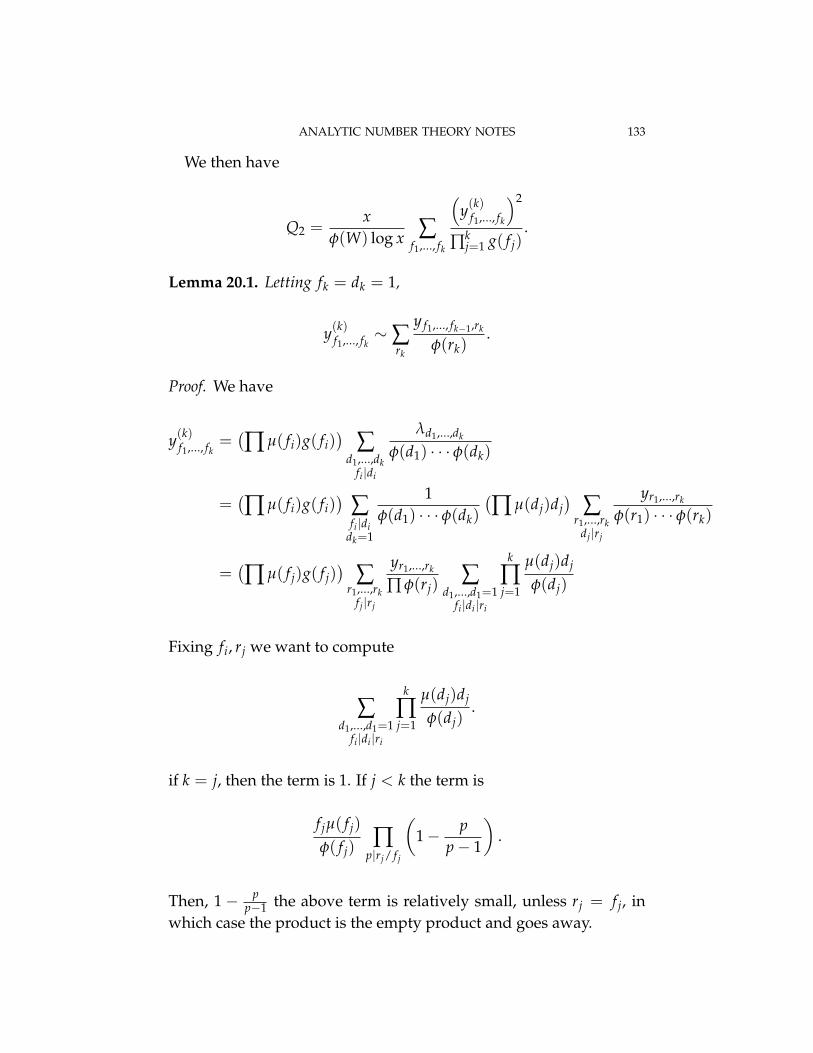
ANALYTIC NUMBER THEORY NOTES 133
We then have
Q2 =x
φ(W) log x ∑f1,..., fk
(y(k)f1,..., fk
)2
∏kj=1 g( f j)
.
Lemma 20.1. Letting fk = dk = 1,
y(k)f1,..., fk∼∑
rk
y f1,..., fk−1,rk
φ(rk).
Proof. We have
y(k)f1,..., fk=(∏ µ( fi)g( fi)
)∑
d1,...,dkfi|di
λd1,...,dk
φ(d1) · · · φ(dk)
=(∏ µ( fi)g( fi)
)∑fi|di
dk=1
1φ(d1) · · · φ(dk)
(∏ µ(dj)dj
)∑
r1,...,rkdj|rj
yr1,...,rk
φ(r1) · · · φ(rk)
=(∏ µ( f j)g( f j)
)∑
r1,...,rkf j|rj
yr1,...,rk
∏ φ(rj)∑
d1,...,d1=1fi|di|ri
k
∏j=1
µ(dj)dj
φ(dj)
Fixing fi, rj we want to compute
∑d1,...,d1=1
fi|di|ri
k
∏j=1
µ(dj)dj
φ(dj).
if k = j, then the term is 1. If j < k the term is
f jµ( f j)
φ( f j)∏
p|rj/ f j
(1− p
p− 1
).
Then, 1− pp−1 the above term is relatively small, unless rj = f j, in
which case the product is the empty product and goes away.
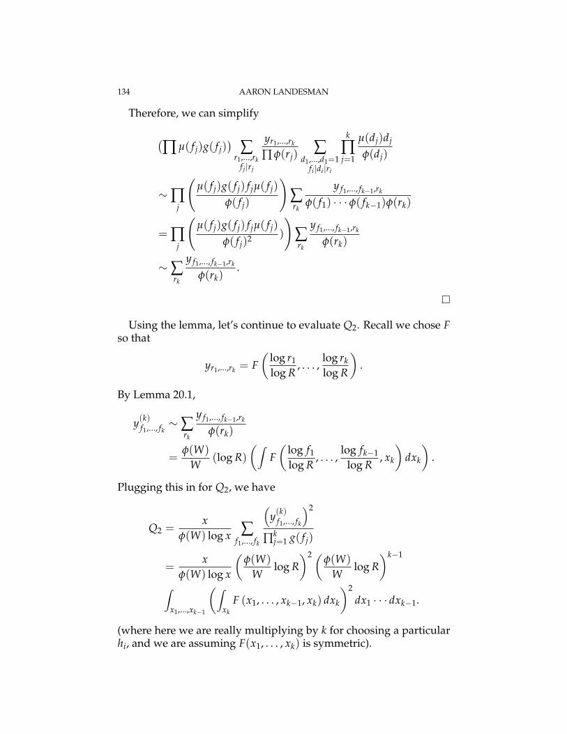
134 AARON LANDESMAN
Therefore, we can simplify
(∏ µ( f j)g( f j)
)∑
r1,...,rkf j|rj
yr1,...,rk
∏ φ(rj)∑
d1,...,d1=1fi|di|ri
k
∏j=1
µ(dj)dj
φ(dj)
∼∏j
(µ( f j)g( f j) f jµ( f j)
φ( f j)
)∑rk
y f1,..., fk−1,rk
φ( f1) · · · φ( fk−1)φ(rk)
= ∏j
(µ( f j)g( f j) f jµ( f j)
φ( f j)2 )
)∑rk
y f1,..., fk−1,rk
φ(rk)
∼∑rk
y f1,..., fk−1,rk
φ(rk).
�
Using the lemma, let’s continue to evaluate Q2. Recall we chose Fso that
yr1,...,rk = F(
log r1
log R, . . . ,
log rklog R
).
By Lemma 20.1,
y(k)f1,..., fk∼∑
rk
y f1,..., fk−1,rk
φ(rk)
=φ(W)
W(log R)
(∫F(
log f1
log R, . . . ,
log fk−1
log R, xk
)dxk
).
Plugging this in for Q2, we have
Q2 =x
φ(W) log x ∑f1,..., fk
(y(k)f1,..., fk
)2
∏kj=1 g( f j)
=x
φ(W) log x
(φ(W)
Wlog R
)2 (φ(W)
Wlog R
)k−1
∫x1,...,xk−1
(∫xk
F (x1, . . . , xk−1, xk) dxk
)2
dx1 · · · dxk−1.
(where here we are really multiplying by k for choosing a particularhi, and we are assuming F(x1, . . . , xk) is symmetric).
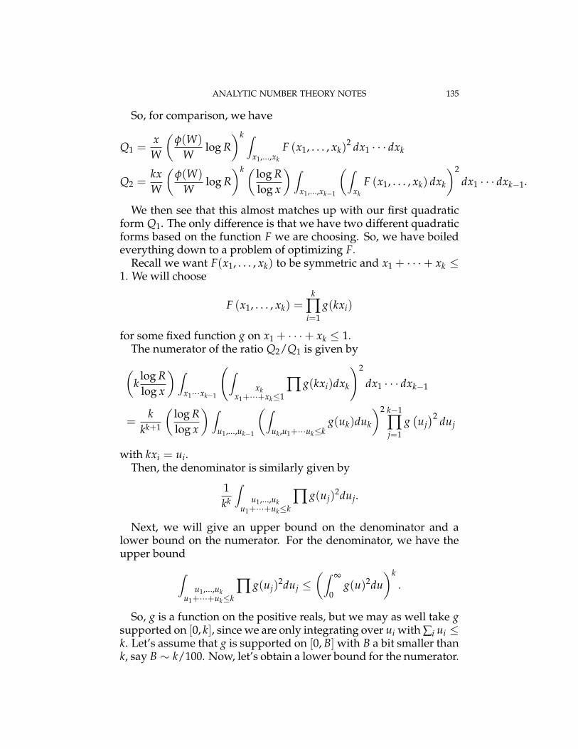
ANALYTIC NUMBER THEORY NOTES 135
So, for comparison, we have
Q1 =x
W
(φ(W)
Wlog R
)k ∫x1,...,xk
F (x1, . . . , xk)2 dx1 · · · dxk
Q2 =kxW
(φ(W)
Wlog R
)k ( log Rlog x
) ∫x1,...,xk−1
(∫xk
F (x1, . . . , xk) dxk
)2
dx1 · · · dxk−1.
We then see that this almost matches up with our first quadraticform Q1. The only difference is that we have two different quadraticforms based on the function F we are choosing. So, we have boiledeverything down to a problem of optimizing F.
Recall we want F(x1, . . . , xk) to be symmetric and x1 + · · ·+ xk ≤1. We will choose
F (x1, . . . , xk) =k
∏i=1
g(kxi)
for some fixed function g on x1 + · · ·+ xk ≤ 1.The numerator of the ratio Q2/Q1 is given by(k
log Rlog x
) ∫x1···xk−1
(∫xk
x1+···+xk≤1∏ g(kxi)dxk
)2
dx1 · · · dxk−1
=k
kk+1
(log Rlog x
) ∫u1,...,uk−1
(∫uk,u1+···uk≤k
g(uk)duk
)2 k−1
∏j=1
g(uj)2 duj
with kxi = ui.Then, the denominator is similarly given by
1kk
∫u1,...,uk
u1+···+uk≤k∏ g(uj)
2duj.
Next, we will give an upper bound on the denominator and alower bound on the numerator. For the denominator, we have theupper bound∫
u1,...,uku1+···+uk≤k
∏ g(uj)2duj ≤
(∫ ∞
0g(u)2du
)k.
So, g is a function on the positive reals, but we may as well take gsupported on [0, k], since we are only integrating over ui with ∑i ui ≤k. Let’s assume that g is supported on [0, B] with B a bit smaller thank, say B ∼ k/100. Now, let’s obtain a lower bound for the numerator.
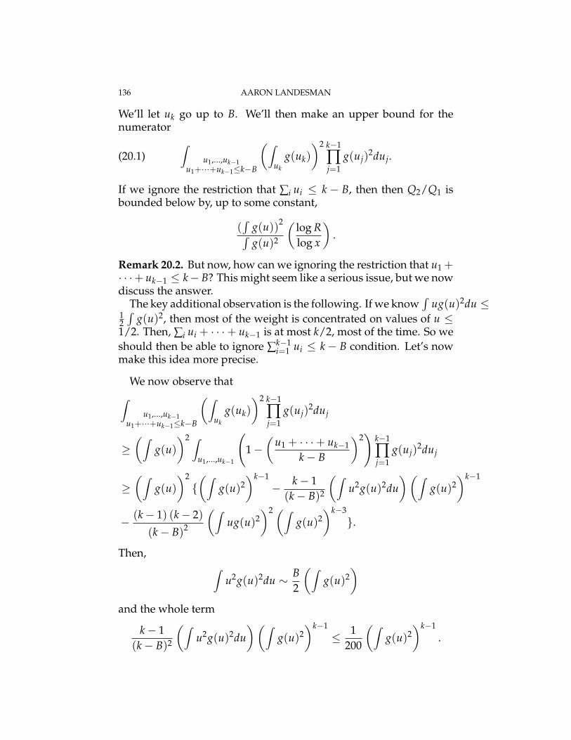
136 AARON LANDESMAN
We’ll let uk go up to B. We’ll then make an upper bound for thenumerator ∫
u1,...,uk−1u1+···+uk−1≤k−B
(∫uk
g(uk)
)2 k−1
∏j=1
g(uj)2duj.(20.1)
If we ignore the restriction that ∑i ui ≤ k − B, then then Q2/Q1 isbounded below by, up to some constant,
(∫
g(u))2∫g(u)2
(log Rlog x
).
Remark 20.2. But now, how can we ignoring the restriction that u1 +· · ·+ uk−1 ≤ k− B? This might seem like a serious issue, but we nowdiscuss the answer.
The key additional observation is the following. If we know∫
ug(u)2du ≤12
∫g(u)2, then most of the weight is concentrated on values of u ≤
1/2. Then, ∑i ui + · · ·+ uk−1 is at most k/2, most of the time. So weshould then be able to ignore ∑k−1
i=1 ui ≤ k− B condition. Let’s nowmake this idea more precise.
We now observe that∫u1,...,uk−1
u1+···+uk−1≤k−B
(∫uk
g(uk)
)2 k−1
∏j=1
g(uj)2duj
≥(∫
g(u))2 ∫
u1,...,uk−1
(1−
(u1 + · · ·+ uk−1
k− B
)2)
k−1
∏j=1
g(uj)2duj
≥(∫
g(u))2
{(∫
g(u)2)k−1
− k− 1(k− B)2
(∫u2g(u)2du
)(∫g(u)2
)k−1
− (k− 1) (k− 2)
(k− B)2
(∫ug(u)2
)2(∫g(u)2
)k−3
}.
Then, ∫u2g(u)2du ∼ B
2
(∫g(u)2
)and the whole term
k− 1(k− B)2
(∫u2g(u)2du
)(∫g(u)2
)k−1
≤ 1200
(∫g(u)2
)k−1
.
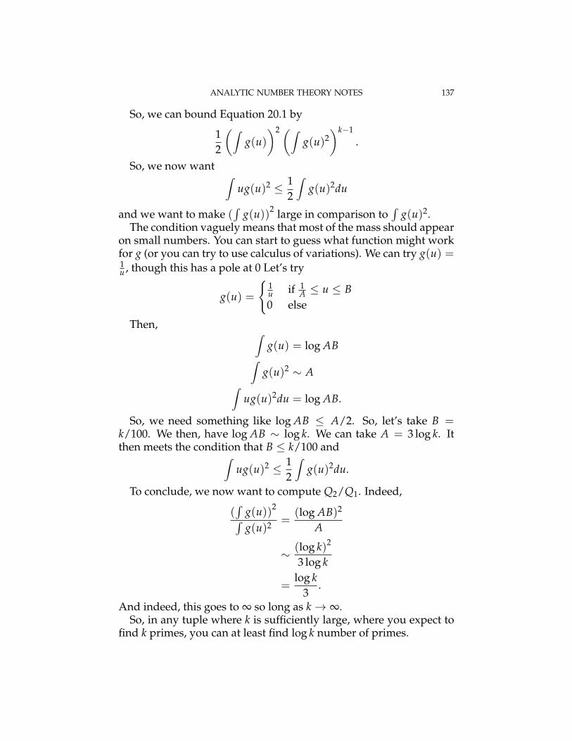
ANALYTIC NUMBER THEORY NOTES 137
So, we can bound Equation 20.1 by
12
(∫g(u)
)2(∫g(u)2
)k−1
.
So, we now want ∫ug(u)2 ≤ 1
2
∫g(u)2du
and we want to make (∫
g(u))2 large in comparison to∫
g(u)2.The condition vaguely means that most of the mass should appear
on small numbers. You can start to guess what function might workfor g (or you can try to use calculus of variations). We can try g(u) =1u , though this has a pole at 0 Let’s try
g(u) =
{1u if 1
A ≤ u ≤ B0 else
Then, ∫g(u) = log AB∫
g(u)2 ∼ A∫ug(u)2du = log AB.
So, we need something like log AB ≤ A/2. So, let’s take B =k/100. We then, have log AB ∼ log k. We can take A = 3 log k. Itthen meets the condition that B ≤ k/100 and∫
ug(u)2 ≤ 12
∫g(u)2du.
To conclude, we now want to compute Q2/Q1. Indeed,
(∫
g(u))2∫g(u)2 =
(log AB)2
A
∼ (log k)2
3 log k
=log k
3.
And indeed, this goes to ∞ so long as k→ ∞.So, in any tuple where k is sufficiently large, where you expect to
find k primes, you can at least find log k number of primes.