analytic properties of potts and ising model partition

Analytic Properties of Potts and

Ising Model Partition Functions

and the Relationship between

Analytic Properties and Phase

Transitions in Equilibrium

Statistical Mechanics

Siti Fatimah Binti Zakaria

Submitted in accordance with the requirements for the degree of

Doctor of Philosophy

The University of Leeds

School of Mathematics

November 2016

The candidate confirms that the work submitted is his/her/their

own and that appropriate credit has been given where reference has

been made to the work of others.

This copy has been supplied on the understanding that it is

copyright material and that no quotation from the thesis may be

published without proper acknowledgement.

@2016 The University of Leeds and Siti Fatimah Binti Zakaria

ii

For my parents and family −

my late father Zakaria Zainal Abidin,

my mother Ramah Mohamad,

and my siblings

Kadir, Hafiz, Arif, and Maznah.

iii

Acknowledgements

In the name of Allah The Most Gracious and The Most Merciful.

First and foremost, I would like to express my biggest appreciation to my

supervisor, Professor Paul Purdon Martin, for his thoughtful guidance and warm

encouragement throughout my Ph.D journey. This research and thesis would not

be possible without him. To me, his patience and encouragement are my greatest

motivation to keep me strong and compose while being in this journey.

I wish to express my gratitude to Dr Mike Evans, my advisor, for his thoughtful

comment especially when I just started my Ph.D. I thank Dr Sandro Azaele (Ph.D

transfer assessor) and Dr Alison Parker (second year assessor) for their thought while

monitoring my study progress and also to Professor Frank Nijhoff and Professor Uwe

Grimm for letting my defence to be an enjoyable experience for me. I specially thank

Dr Zoltan Kadar for the time he spent reviewing my thesis and also to Professor

Michael E. Fisher for sending me a part of his lecture notes on the ‘Fisher zero’.

I would like to also take this opportunity to thank my sponsors, the Ministry

of Higher Education Malaysia and the International Islamic University Malaysia.

Thank you for giving me the opportunity to further my study and also for supporting

me financially.

Also not to forget, my appreciation to all my colleagues and friends in School

of Mathematics for making my journey less lonely - especially Huda, Nada, Diana,

Mufida, Amani, Eman, Chwas, Ahmed, Raphael, Alex, Konstant, Taysir, Khawlah,

and Areena. I also want to thank Craig Hall for his help in setting up my dual-boot

computer during my first year.

v

To my close friends especially Dr Rozaimah, Dr Ummu Atiqah, Fairuz Alwani,

Afifah Hanum, Saidatun Nisa’, Faieqah, Sarah, K. Fairuz, Syikin, Ernest, K. Juniza,

and Fatin, I thank all of you for always be with me from the beginning of my study

until the end.

Finally, my special and endless appreciation for my family especially my late

father, my mother, and also my brothers and sister for their prayers and support.

Words cannot describe how grateful I am for all the sacrifices they have made on

my behalf.

Thank you so much for everything. May God bless us.

vi

Abstract

The Ising and Q-state Potts models are statistical mechanical models of spins

interaction on crystal lattices. We study the partition functions on a range of

lattices, particularly two- and three-dimensional cases. The study aims to investigate

cooperative phenomena − how higher level structure is affected by the detailed

activity of a very large number of lower level structures. We investigate the analytic

properties of the partition functions and their relationship to physical observables in

equilibrium near phase transition. Our study is focussed on describing the partition

function and the distribution of zeros of the partition function in the complex-

temperature plane close to phase transitions. Here we first consider the solved case

of the Ising model on square lattice as a benchmark for checking our method of

computation and analysis. The partition function is computed using a transfer

matrix approach and the zeros are found numerically by Newton-Raphson method.

We extend the study of Q-state Potts models to a more general case called the ZQ-

symmetric model. We evidence the existence of multiple phase transitions for this

model in case Q = 5, 6, and discuss the possible connection to different stages of

disordered state. Given sufficient and efficient coding and computing resources, we

extend many previously studied cases to larger lattice sizes. Our analysis of zeros

distribution close to phase transition point is based on a certain power law relation

which leads to critical exponent of physical observable. We evidence for example,

that our method can be used to give numerical estimates of the specific heat critical

exponent α.

vii

Contents

Dedication . . . . . . . . . . . . . . . . . . . . . . . . . . . . . . . . . . . . iii

Acknowledgements . . . . . . . . . . . . . . . . . . . . . . . . . . . . . . . v

Abstract . . . . . . . . . . . . . . . . . . . . . . . . . . . . . . . . . . . . . vii

Contents . . . . . . . . . . . . . . . . . . . . . . . . . . . . . . . . . . . . . ix

List of figures . . . . . . . . . . . . . . . . . . . . . . . . . . . . . . . . . . xiii

List of tables . . . . . . . . . . . . . . . . . . . . . . . . . . . . . . . . . . xxi

Nomenclature . . . . . . . . . . . . . . . . . . . . . . . . . . . . . . . . . . xxiii

1 Introduction 1

1.1 The Potts models − definitions . . . . . . . . . . . . . . . . . . . . . 2

1.2 Partition Function Z . . . . . . . . . . . . . . . . . . . . . . . . . . . 4

1.3 Relation to physical observables . . . . . . . . . . . . . . . . . . . . . 6

1.4 Physical motivation . . . . . . . . . . . . . . . . . . . . . . . . . . . . 8

1.4.1 Ising and Potts models . . . . . . . . . . . . . . . . . . . . . . 8

1.4.2 ZQ-symmetric model . . . . . . . . . . . . . . . . . . . . . . . 8

1.4.3 Onsager’s solution . . . . . . . . . . . . . . . . . . . . . . . . 9

1.4.4 What can be computed and what it means . . . . . . . . . . . 10

1.4.5 Phase transition − example of physical phenomena . . . . . . 11

1.5 Objectives and Aims . . . . . . . . . . . . . . . . . . . . . . . . . . . 11

2 Models on lattice 15

2.1 Graph of regular lattice . . . . . . . . . . . . . . . . . . . . . . . . . . 15

2.1.1 Thermodynamic limit . . . . . . . . . . . . . . . . . . . . . . . 16

ix

x Contents

2.1.2 Lattice graph . . . . . . . . . . . . . . . . . . . . . . . . . . . 16

2.1.2.1 d-dimensional lattice . . . . . . . . . . . . . . . . . . 17

2.1.2.2 Dense sphere packing . . . . . . . . . . . . . . . . . . 18

2.1.3 Boundary condition . . . . . . . . . . . . . . . . . . . . . . . . 21

2.2 Duality . . . . . . . . . . . . . . . . . . . . . . . . . . . . . . . . . . . 23

2.2.1 Z in dichromatic polynomial . . . . . . . . . . . . . . . . . . . 25

2.2.2 Duality relation for partition function . . . . . . . . . . . . . . 30

3 Computation for partition function 33

3.1 Models on lattice − example . . . . . . . . . . . . . . . . . . . . . . . 33

3.2 Partition Vector and Transfer Matrix . . . . . . . . . . . . . . . . . . 35

3.2.1 Transfer matrix . . . . . . . . . . . . . . . . . . . . . . . . . . 38

3.2.2 Boundary Condition . . . . . . . . . . . . . . . . . . . . . . . 41

3.2.3 Symmetry on graph . . . . . . . . . . . . . . . . . . . . . . . . 42

3.3 Zeros of partition function . . . . . . . . . . . . . . . . . . . . . . . . 45

4 Square lattice Ising model partition function zeros 47

4.1 Exact solution − the Onsager’s solution . . . . . . . . . . . . . . . . 48

4.2 Ising model on finite lattice case . . . . . . . . . . . . . . . . . . . . . 54

4.3 Finite size effect . . . . . . . . . . . . . . . . . . . . . . . . . . . . . . 57

4.4 Duality relation . . . . . . . . . . . . . . . . . . . . . . . . . . . . . . 60

4.5 Ferromagnetic and antiferromagnetic regions . . . . . . . . . . . . . . 61

5 The Q-state Potts model partition function zeros 63

5.1 2-state Potts (Ising) model on square lattice − revisited . . . . . . . . 67

5.1.1 The effect of boundary conditions . . . . . . . . . . . . . . . . 68

5.2 3-state Potts model on square lattice . . . . . . . . . . . . . . . . . . 74

5.2.1 Self-duality partition function . . . . . . . . . . . . . . . . . . 82

5.3 Q ≥ 4, square lattice Potts model . . . . . . . . . . . . . . . . . . . . 85

5.4 On triangular and hexagonal lattice . . . . . . . . . . . . . . . . . . . 89

Contents xi

5.4.1 Duality transformation . . . . . . . . . . . . . . . . . . . . . . 96

5.5 On cubic lattice . . . . . . . . . . . . . . . . . . . . . . . . . . . . . . 100

5.6 On tetragonal and octagonal lattice . . . . . . . . . . . . . . . . . . . 105

5.7 Discussion . . . . . . . . . . . . . . . . . . . . . . . . . . . . . . . . . 110

6 The ZQ-symmetric model partition function zeros 113

6.1 ZQ-symmetric model − definitions . . . . . . . . . . . . . . . . . . . . 114

6.2 The zeros distribution on square lattice . . . . . . . . . . . . . . . . . 119

6.2.1 5-state: Z5-symmetric . . . . . . . . . . . . . . . . . . . . . . 120

6.2.2 6-state: Z6-symmetric . . . . . . . . . . . . . . . . . . . . . . 131

6.3 Discussion . . . . . . . . . . . . . . . . . . . . . . . . . . . . . . . . . 137

6.3.1 Energy losses in configurations . . . . . . . . . . . . . . . . . . 141

7 Analysis on zeros density of partition function 145

7.1 The specific heat critical exponent . . . . . . . . . . . . . . . . . . . 146

7.2 Zeros and α-exponent . . . . . . . . . . . . . . . . . . . . . . . . . . . 148

7.3 Analysis on zeros density distribution . . . . . . . . . . . . . . . . . . 151

7.3.1 The 2-state Potts model and Ising model − finite case from

Onsager’s solution . . . . . . . . . . . . . . . . . . . . . . . . 153

7.3.2 The 3-state Potts model . . . . . . . . . . . . . . . . . . . . . 162

7.3.3 The accumulated case of 3-state Potts model . . . . . . . . . . 166

8 Analytical machinery for multiple phases in ZQ-symmetric model 171

8.1 Candidates for 3 phase models . . . . . . . . . . . . . . . . . . . . . . 171

8.2 Energy vs entropy . . . . . . . . . . . . . . . . . . . . . . . . . . . . . 172

8.2.1 Single order/disorder phase transition . . . . . . . . . . . . . . 172

8.2.2 Two phase transitions . . . . . . . . . . . . . . . . . . . . . . 173

8.3 ZQ-symmetric model partition function . . . . . . . . . . . . . . . . . 175

8.3.1 Individual term of partition function polynomial . . . . . . . . 176

8.3.2 The picture of polynomial term contribution . . . . . . . . . . 176

xii Contents

8.4 Graph comparison of specific heat . . . . . . . . . . . . . . . . . . . . 190

8.4.1 2- and 3-state Potts models’ specific heat . . . . . . . . . . . . 190

8.4.2 Z5- and Z6-symmetric models’ specific heat . . . . . . . . . . . 192

8.5 Discussion . . . . . . . . . . . . . . . . . . . . . . . . . . . . . . . . . 194

Conclusion 197

Appendix 199

A Algorithm for zeros finding . . . . . . . . . . . . . . . . . . . . . . . . 199

A.1 On error estimation . . . . . . . . . . . . . . . . . . . . . . . . 200

A.2 Refinement and convergence . . . . . . . . . . . . . . . . . . . 201

B Onsager’s solution . . . . . . . . . . . . . . . . . . . . . . . . . . . . . 203

C Coefficient of partition function . . . . . . . . . . . . . . . . . . . . . 207

Bibliography 217

List of Figures

1.1 Bar magnet and its magnetic dipoles in cubic lattice. . . . . . . . . . 2

1.2 Square lattices with different system size N by M . . . . . . . . . . . . 9

1.3 Specific heat of square lattice Ising model (Onsager’s solution). . . . . 12

1.4 3-state Potts model on 15 by 17 square lattice. . . . . . . . . . . . . . 13

2.1 The one-dimensional lattice of N sites. . . . . . . . . . . . . . . . . . 17

2.2 Square lattice N by N for N = 2, 3, 4. . . . . . . . . . . . . . . . . . . 17

2.3 Triangular lattice. . . . . . . . . . . . . . . . . . . . . . . . . . . . . . 18

2.4 Hexagonal lattice (left) to rectangular graph layering (right) for

computer program. . . . . . . . . . . . . . . . . . . . . . . . . . . . . 19

2.5 Cubic lattice. . . . . . . . . . . . . . . . . . . . . . . . . . . . . . . . 19

2.6 Octagonal lattice i.e. face-centered cubic lattice. . . . . . . . . . . . . 19

2.7 Tetragonal lattice i.e. hexagonal close-packed lattice. . . . . . . . . . 19

2.8 Structure showing the face-centered cubic lattice point arrangement

in a unit cell. . . . . . . . . . . . . . . . . . . . . . . . . . . . . . . . 20

2.9 Face-centered cubic, hexagonal close-packed and their stacking

sequence respectively. . . . . . . . . . . . . . . . . . . . . . . . . . . 21

2.10 4 by 2 square lattice with periodic boundary condition in vertical

direction. . . . . . . . . . . . . . . . . . . . . . . . . . . . . . . . . . 22

2.11 Increasing sizes of square lattices. The red sites highlight the spins

at boundary and the black sites are the interior sites. . . . . . . . . . 23

2.12 Square lattice and its dual. . . . . . . . . . . . . . . . . . . . . . . . . 25

xiii

xiv List of Figures

2.13 Hexagonal lattice and its dual, a triangular lattice. . . . . . . . . . . 25

2.14 Self-dual square lattice. . . . . . . . . . . . . . . . . . . . . . . . . . . 26

2.15 Set of bonds EG′ can be illustrated by bond 0 and 1. . . . . . . . . . 27

2.16 Example of connected cluster including its isolated vertices with

a)|C(G′)| = 4 and b)|C(G′)| = 3. . . . . . . . . . . . . . . . . . . . . 28

2.17 Examples of non-even bond covering. . . . . . . . . . . . . . . . . . . 29

3.1 2 by 2 square lattices. . . . . . . . . . . . . . . . . . . . . . . . . . . . 34

3.2 2 by 2 square lattice. . . . . . . . . . . . . . . . . . . . . . . . . . . . 38

3.3 Lattice graphs G,G′ and GG′ where G and G′ connected to form

GG′. The dot circles represent the incoming and outgoing spins, for

example, ViG and VOG respectively. . . . . . . . . . . . . . . . . . . . 39

3.4 5 by 5 square lattice with periodic boundary in vertical direction. . . 41

3.5 4 by 2 square lattice with periodic boundary condition in vertical

direction. . . . . . . . . . . . . . . . . . . . . . . . . . . . . . . . . . 44

4.1 Square lattice with local bond construction. . . . . . . . . . . . . . . 49

4.2 Zeros plane for 14 by 14 square lattice, a) complete distribution and

b) a blow up picture near real axis. . . . . . . . . . . . . . . . . . . . 55





4.5 Zeros plane for 100 by 100 square lattice, a) complete distribution

and b) a blow up picture near real axis. . . . . . . . . . . . . . . . . . 56

4.6 ∞×∞ square lattice Ising model. . . . . . . . . . . . . . . . . . . . 56

4.7 Zeros plane for N = 10, 20, 50 and 70. . . . . . . . . . . . . . . . . . . 58

4.8 Overlay distributions on square lattices with different system size N . 59

4.9 Overlay distributions on cubic lattices with different system size N . . 59

List of Figures xv

4.10 Distribution of dual zeros for 14 by 14 Ising square lattice and the

circle (4.16). . . . . . . . . . . . . . . . . . . . . . . . . . . . . . . . . 61

5.1 Number of row vertices denoted y (also we denote this y = N) and

column vertices denoted x (also we denote this x = M). . . . . . . . . 64

5.2 Square lattice Ising model with Onsager’s partition function a) 14×14

and b) 50× 50. . . . . . . . . . . . . . . . . . . . . . . . . . . . . . . 67

5.3 ∞×∞ square lattice Ising model. . . . . . . . . . . . . . . . . . . . 67

5.4 2-state, square lattice with periodic-open boundary conditions. . . . . 69

5.5 2-state, square lattice with periodic-open boundary conditions (cont.). 70

5.6 Zeros distributions for N = 8, 14 square lattices: ons-8 × 8 and ons-

14× 14 are generated from the Onsager’s partition function (4.13). . 71

5.7 2-state, square lattice with periodic-periodic boundary conditions. . . 71

5.8 2-state, square lattice with self-dual boundary conditions. . . . . . . . 72

5.9 2-state, square lattice with different boundary conditions. . . . . . . . 73






5.15 3-state Potts model on a) 12× 12′ and 13× 13′ and b) 14× 14′ and

15× 17′ square lattices. . . . . . . . . . . . . . . . . . . . . . . . . . . 78

5.16 Antiferro [0,1]-region: 3-state Potts model on N = 12, 13, 14, 15

square lattices. . . . . . . . . . . . . . . . . . . . . . . . . . . . . . . 79

5.17 Zoom in: 3-state Potts model on 12× 12′ and 13× 13′ square lattices. 80

5.18 Zoom in: 3-state Potts model on 14× 14′ and 15× 17′ square lattices. 81

5.19 Zeros distribution for polynomial Z∗: a) N = 12 and b) N = 13. . . . 83

5.20 Zeros distribution for polynomial Z,Zd and Z∗ = Z ′: a) N = 14 and

b) N = 15. . . . . . . . . . . . . . . . . . . . . . . . . . . . . . . . . . 84

xvi List of Figures


5.22 4-state, square lattice with periodic-open boundary conditions (cont.). 86



5.25 2-state, triangular lattice with periodic-open boundary conditions. . . 90

5.26 2-state, triangular lattice with periodic-open boundary conditions

(cont.). . . . . . . . . . . . . . . . . . . . . . . . . . . . . . . . . . . . 91




5.30 2-state, hexagonal lattice with periodic-open boundary conditions. . . 95



5.33 2-state, duality transformation of 11 by 11 triangular lattice with

periodic-open boundary conditions. . . . . . . . . . . . . . . . . . . . 98







5.37 2-state, cubic lattice with periodic-periodic-open boundary conditions. 100

5.38 2-state, cubic lattice with periodic-periodic-open boundary conditions

(cont.). . . . . . . . . . . . . . . . . . . . . . . . . . . . . . . . . . . . 101





5.43 2-state, tetragonal lattice with periodic-open boundary conditions. . . 107

List of Figures xvii

5.44 3-state, tetragonal lattice with periodic-open boundary conditions. . . 108

5.45 2-state, octagonal lattice with periodic-open boundary conditions. . . 109

5.46 3-state, octagonal lattice with periodic-open boundary conditions. . . 110

6.1 The interaction of a spin relative to spin 1 represented by a pair of

arrow. . . . . . . . . . . . . . . . . . . . . . . . . . . . . . . . . . . . 114

6.2 The illustration of energy list with: (a) χa = (1, γ1, 0), (b) χb =

(1, γ1, 0), and (c) χc = (1, γ1, γ2, 0). . . . . . . . . . . . . . . . . . . . 117

6.3 The illustration of Z4-symmetric model with energy value χ =

(1, 2/3, 0) (left) and χ = 3χ = (3, 2, 0) (right). . . . . . . . . . . . . . 118

6.4 Zeros distribution for χ = (2, 1, 0) 5-state model. . . . . . . . . . . . . 121









6.13 Zeros distribution for χ = (2, 1, 0, 0) 6-state model. . . . . . . . . . . 132





6.18 Zeros distribution for several χ of 6 by 6 on square lattice. . . . . . . 139

6.19 Zeros distribution for several χ of 6 by 6 on square lattice (cont.). . . 140

6.20 a) Value of spin configurations associated to the lattice sites and b)

regions of aligned spin configurations. . . . . . . . . . . . . . . . . . . 141

6.21 A configuration with fixed boundary condition. . . . . . . . . . . . . 142

xviii List of Figures

7.1 Phase change diagram. . . . . . . . . . . . . . . . . . . . . . . . . . 146

7.2 Specific heat of square lattice Ising model (Onsager’s solution). . . . . 147

7.3 Specific heat in the 3-state Potts model on square lattice with lattice

sizes, N = 12, 13, 15. . . . . . . . . . . . . . . . . . . . . . . . . . . . 148

7.4 Example: first quadrant with bin of equal size for square lattice Ising

model, N = 50. . . . . . . . . . . . . . . . . . . . . . . . . . . . . . . 152

7.5 Lattice 19× 19 : Linear regression analysis on log-log graphs. . . . . 154





7.10 Lattice 100× 100 : Linear regression analysis on log-log graphs. . . . 161

7.11 Zeros distribution at quadrant 1 for 3-state Potts model on square

lattice of a) 12 by 12, b) 13 by 13, c) 14 by 14 and d) 15 by 17. . . . 163

7.12 Lattice 12x12 : Linear regression analysis on log-log graphs. . . . . . 163




7.16 Lattice 12 × 12′ to 15 × 17′ : Linear regression analysis on log-log

graphs. . . . . . . . . . . . . . . . . . . . . . . . . . . . . . . . . . . . 167

7.17 Lattice 12 × 12′ to 15 × 17′ : Linear regression analysis on log-log

graphs (cont.). . . . . . . . . . . . . . . . . . . . . . . . . . . . . . . . 168

8.1 The 8 by 8 zeros distribution for a) χ = (3, 1, 0) and b) χ = (3, 2, 0). . 172

8.2 Example of vortex-antivortex pair with a) smooth line separation and

b) rough line separation. . . . . . . . . . . . . . . . . . . . . . . . . . 174

8.3 Illustration of some zeros of Z for the first, second and third closest

to the positive real axis. . . . . . . . . . . . . . . . . . . . . . . . . . 174

List of Figures xix

8.4 Example of configuration and line separation on dual lattice with a)

1 spin flip and b) 2 same spin flip. . . . . . . . . . . . . . . . . . . . . 176

8.5 2-state Potts model on 18 by 18 square lattice with a) x1 = 2.42196+

.0287144 I, b) x2 = 2.42216 + 0.462357 I, c) x3 = 2.26734 + 0.641372 I.178

8.6 Zeros distribution for a) x = eβJ and b) x = e−βJ with χ = (3, 2, 0). . 179

8.7 Z5-symmetric model on 8 by 8 square lattice with χ = (2, 1, 0): a)

x1 = 2.10969 + 0.479109 I, b) x2 = 2.42248 + 0.665705 I and c) x3 =

2.07525 + 0.734082 I. . . . . . . . . . . . . . . . . . . . . . . . . . . . 180

8.8 Z5-symmetric model on 8 by 8 square lattice with χ = (3, 1, 0): a)

x1 = 1.62980 + 0.137975 I, b) x2 = 1.62659 + 0.205334 I and c) x3 =

1.61877 + 0.270632 I. . . . . . . . . . . . . . . . . . . . . . . . . . . . 181

8.9 First curve: Z5-symmetric model on 8 by 8 square lattice with χ =

(3, 2, 0): a) x1 = 1.64360 + 0.334788 I, b) x2 = 1.58838 + 0.476209 I

and c) x3 = 1.37846 + 0.546351 I. . . . . . . . . . . . . . . . . . . . . 182

8.10 Second curve: Z5-symmetric model on 8 by 8 square lattice with χ =

(3, 2, 0): a) x = 2.36582 + 0.771200 I and b) x = 2.24748 + 0.114699 I. 182

8.11 Polynomial range categorisation for x. . . . . . . . . . . . . . . . . . 183

8.12 Zeros distribution for x = e−βJ with a) χ = (3, 2, 0, 0) and b) χ =

(3, 2, 1, 0). . . . . . . . . . . . . . . . . . . . . . . . . . . . . . . . . . 184

8.13 Zeros distribution for x = eβJ with χ = (2, 1, 0, 0). . . . . . . . . . . . 185

8.14 Z6-symmetric model on 8 by 8 square lattice with χ = (2, 1, 0, 0):

a) x = 2.08847 + 0.405804 I, b) x = 2.08267 + 0.622161 I and c)

x = 2.42583 + 0.658524 I. . . . . . . . . . . . . . . . . . . . . . . . . 186

8.15 Zeros distribution for x = eβJ with χ = (3, 2, 0, 0). . . . . . . . . . . . 186


a) x = 1.64122 + 0.123280 I, b) x = 1.64234 + 0.186484 I and c)

x = 1.63573 + 0.247940 I. . . . . . . . . . . . . . . . . . . . . . . . . 187

xx List of Figures

8.17 First curve: Z6-symmetric model on 8 by 8 square lattice with χ =

(3, 2, 0, 0): a) x = 1.60486 + 0.259279 I, b) x = 1.58125 + 0.37801 I

and c) x = 1.41710 + 0.486042 I. . . . . . . . . . . . . . . . . . . . . 188

8.18 Second curve: Z6-symmetric model on 8 by 8 square lattice with χ =

(3, 2, 0, 0): a) x = 2.36594 + 0.771063 I and b) x = 2.2475 + 1.14668 I. 188


a) x = 1.85197 + 0.390385 I, b) x = 1.81864 + 0.584863 I and c)

x = 2.43082 + 0.682177 I. . . . . . . . . . . . . . . . . . . . . . . . . 189

8.20 Specific heat plot forCVkB

vs β with N = 16, 18, 20. . . . . . . . . . . 191

8.21 Specific heat plot forCVkB

vs β with N = 12, 13, 15. . . . . . . . . . . 191

8.22 Z5-symmetric model: Specific heat graph for a) 8 × 8 with different

χ and b) 7× 9, 8× 8, 9× 9 for χ = (3, 2, 0). . . . . . . . . . . . . . . 192

8.23 Z6-symmetric model: Specific heat graph on square lattice a) 8 × 8

with different χ and b) 6× 7, 7× 7, 8× 8 for χ = (3, 2, 0, 0). . . . . . 193

8.24 Ordered-disordered states illustration (not scaled). . . . . . . . . . . . 195

List of Tables

5.1 Largest sizes for all considered lattice types including the new results

(highlighted in grey). . . . . . . . . . . . . . . . . . . . . . . . . . . . . 64

6.1 gr(σ(j), σ(k)) for Z3-symmetric model. . . . . . . . . . . . . . . . . . 115

6.2 g′r(σ(j), σ(k)) for Z3-symmetric model. . . . . . . . . . . . . . . . . . 116

6.3 The Z5- and Z6-symmetric models with arbitrary χ. New results are

highlighted grey. . . . . . . . . . . . . . . . . . . . . . . . . . . . . . 120

7.1 Approximated slope m of log-log plane for 19 × 19′ and 20 × 20′

square lattices. The manual column is our own estimate directly on

the log-log graph. . . . . . . . . . . . . . . . . . . . . . . . . . . . . 153



the log-log graph. . . . . . . . . . . . . . . . . . . . . . . . . . . . . . 155



the log-log graph. . . . . . . . . . . . . . . . . . . . . . . . . . . . . . 156



the log-log graph. . . . . . . . . . . . . . . . . . . . . . . . . . . . . . 162

xxi

xxii List of Tables



the log-log graph. . . . . . . . . . . . . . . . . . . . . . . . . . . . . . 162

7.6 Approximated slope m of log-log plane for accumulated zeros from

12 × 12′, 13 × 13′, 14 × 14′ and 15 × 17′ square lattices. The manual

column is our own estimate directly on the log-log graph. . . . . . . . 166

Nomenclature

Symbols

N Natural numbers

R Real numbers

Q number of spin directions

ZQ cyclic group of order Q

β inverse temperature

T absolute temperature

kB Boltzmann constant

J interaction strength

H,HIsing,HPotts Hamiltonian functions

〈i, j〉 nearest neighbour pair of lattice sites, i and j

σI(i) spin configuration for Ising model at site i

σP (i) spin configuration for Potts model at site i

σi spin configuration at site i

Ω set of all possible configuration states

σ a configuration state, σ ∈ Ω

Z,Z ′, ZIsing, ZPotts partition functions

δij the Kronecker delta symbol

V volume

CV specific heat

Λ,Γ, G graph

xxiii

xxiv Nomenclature

d dimension, d ∈ N

T transfer matrix

P power set

α specific heat exponent

Abbreviations

fcc face-centered cubic

hcp hexagonal close-packed

ferro ferromagnetic

antiferro antiferromagnetic

TOL tolerance or computing error

GMP GNU multiple precision

NR Newton-Raphson method

RAM random accessed memory

Chapter 1

Introduction

This thesis describes our research in statistical mechanics [30, 48, 65]. Statistical

mechanics is an area where mathematical modelling is used to understand a physical

system. In physics, it is a key problem to predict behaviour of a physical system

[35, 46, 101]. This is useful for many applications [18, 43, 85].

Statistical mechanics models the microscopic properties of individual atom and

molecule of a material that can be observed in nature, and relates them to the

macroscopic or bulk properties [35, 96]. We study the statistical mechanical models

of spin variables on a graph, representing the molecular dipoles on the crystal lattice

of a physical system − such as a bar magnet.

One example of physical phenomena which can benefit from the statistical

mechanical study is the event of phase transition [27, 101]. The study helps in

predicting the critical properties of a phase transition by investigating the inner

activity of molecular dipoles in a physical system.

The model in this thesis is a model of ferromagnetism [41, 44–46, 68] on solid

state material that has a crystalline feature on its atomic scale. From experiment

[28, 71, 91, 97], the crystalline structure shows the constituent particles being stack

together in a regular and repeated pattern in R3. This is formed by the translations

of some kind of basic cell, for example the translation of a cube to a cubic lattice

[31].

1

2 Chapter 1

In modelling the effective ferromagnetism, the dynamics of the lattice such as

the vibrational and bulk motion are ignored. Instead, the dynamic is restricted to

the molecular dipoles residing at the lattice sites. The molecular dipole centre of

mass remain fixed in its location. We call the model variable represented by the

molecular dipole as a spin variable of the crystal lattice. Here the degree of freedom

is obtained from the spin orientation. The model is restricted to a system with

identical atomic type. The dipole-dipole interactions are short range [4, 41]. Thus in

the model we put a short range interaction between two neighbouring spin variables.

Here the interaction with external magnetic field is excluded for simplicity. Also for

simplicity, two spin variables interact with each other if they are close together. At

larger distance, the interaction is assumed to be negligible.

Let Q ∈ N be the number of spin orientations. For Q = 2 we consider the Ising

model [37, 62] which also called the 2-state Potts model [3, 79]. For Q > 2 we vary

the model in this thesis by the Q-state Potts model and the ZQ-symmetric model

[58, 83].

Figure 1.1: Bar magnet and its magnetic dipoles in cubic lattice.

1.1 The Potts models − definitions

The Q-state Potts model is a representation of ferromagnetism in which spins are

allowed to be oriented from Q possible spin directions.

The physical spins are assumed to sit at a regular collection of points in R3,

called a lattice. For these models, we represent the lattice by a graph [64]. The spin

variable is associated to the vertex of the graph. The graph vertices can be thought

Chapter 1 3

as the graph embedding to Euclidean space R3. The graph and the Potts model are

defined as below.

Definition 1.1.1 ([19]). A directed graph Λ is a triple Λ = (V,E, f). The V is a

set. The elements v ∈ V are called vertices. The E is also a set. The elements

e ∈ E are called edges. The f is a function f : E → V × V . Given e ∈ E and

v1, v2 ∈ V , the images f(e) = 〈v1, v2〉 gives the ‘source’ and ‘target’ vertex of edge e.

Definition 1.1.2. The distance dΛ(u, v) is the number of edges in the shortest path

from u to v. Two vertices u, v ∈ V are called nearest neighbours if f(e) = 〈u, v〉 for

some e ∈ E i.e. when dΛ(u, v) = 1.

A function σ : V → Q = 1, 2, ..., Q is called a spin configuration for Q-state

Potts models. The value in set Q is the label representing the Q different spin

orientations.

Let Ω be the set of all possible spin configuration states or microstates for a

Q-state Potts model on a given lattice.

Definition 1.1.3 ([49]). Let A,B be sets. Then Hom(A,B) is the set of functions

f : A→ B.

We have immediately;

Theorem 1.1.1. Let Λ = (V,E, f) be a graph and Q ∈ N. Then the configuration

set on graph Λ is Ω = Hom(V,Q).

Thus, for a system of N vertices with Q possible spin directions, the total number

of microstates |Ω| = Q|V | = QN .

In physics, an observable is any physical property of a system which can be

experimentally measured. In a model with given Ω we have a corresponding

operator:

Definition 1.1.4. Consider a physical system in the form of a set Ω. A function

O : Ω→ R is called an observable of the physical system.

4 Chapter 1

One possible observable on a system would be the total energy, also known as

H : Ω → R, or Hamiltonian. It is the form of H which determines what kind

of physical system we are modelling. Let J ∈ R be a constant representing the

interaction strength of the nearest neighbour spins. The Hamiltonian of Potts model

is defined as follows. Let σ ∈ Ω.

Definition 1.1.5. The Hamiltonian of Potts model on Λ = (V,E, f) is defined as

HPotts(σ) = −J∑

〈i,j〉=f(e),e∈E

δσ(i)σ(j) where the Kronecker delta function,

δσ(i)σ(j) =

1, if σ(i) = σ(j)

0, if σ(i) 6= σ(j)

.

The summation is over all the nearest neighbour interaction in Λ.

If J > 0 the system is in its lowest energy where all spin variables are oriented in

the same direction. This state corresponds to a ferromagnetic state. Conversely, if

J < 0 each spin variable is forced to be oriented anti-align to its nearest neighbours.

This state corresponds to an antiferromagnetic state.

1.2 Partition Function Z

Now we are ready to introduce the main function of this thesis. A partition function

denoted as Z is a special function that relates temperature with the states of a spin

system. It provides important information on thermodynamic properties of the

system [35, 58, 101].

Consider an ensemble of similar systems in a heat bath. The heat bath is a body

which has a huge heat capacity that remains its temperature fixed at all times. The

volume, pressure, number of particles and all other properties are assumed to be

fixed except the energy which is allowed to be transferred to its neighbour. So, any

system in contact with the heat bath will eventually reach a thermal equilibrium at

Chapter 1 5

the temperature of the heat bath. This ensemble is called a canonical ensemble [10].

The partition function for a system which allows the transfer of energy to its

environment while fixing other properties is called a canonical partition function or

simply a partition function.

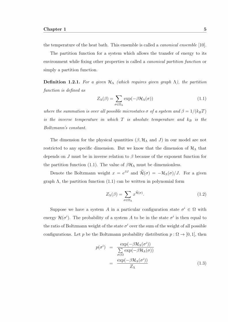
Definition 1.2.1. For a given HΛ (which requires given graph Λ), the partition

function is defined as

ZΛ(β) =∑σ∈ΩΛ

exp(−βHΛ(σ)) (1.1)

where the summation is over all possible microstates σ of a system and β = 1/(kBT )

is the inverse temperature in which T is absolute temperature and kB is the

Boltzmann’s constant.

The dimension for the physical quantities (β,HΛ and J) in our model are not

restricted to any specific dimension. But we know that the dimension of HΛ that

depends on J must be in inverse relation to β because of the exponent function for

the partition function (1.1). The value of βHΛ must be dimensionless.

Denote the Boltzmann weight x = eβJ and H(σ) = −HΛ(σ)/J . For a given

graph Λ, the partition function (1.1) can be written in polynomial form

ZΛ(β) =∑σ∈ΩΛ

xH(σ). (1.2)

Suppose we have a system A in a particular configuration state σi ∈ Ω with

energy H(σi). The probability of a system A to be in the state σi is then equal to

the ratio of Boltzmann weight of the state σi over the sum of the weight of all possible

configurations. Let p be the Boltzmann probability distribution p : Ω→ [0, 1], then

p(σi) =exp(−βHΛ(σi))∑

σ∈Ω

exp(−βHΛ(σ))

=exp(−βHΛ(σi))

ZΛ

(1.3)

6 Chapter 1

where ∑i

p(σi) = 1.

The partition function ZΛ as denominator is also called a normalizing constant. For

simplicity we denote the partition function as Z.

1.3 Relation to physical observables

The role of the partition function Z does not stop at being a normalising constant

as in (1.3) but it also leads to thermodynamic properties. In this section, we present

some of the thermodynamic properties derived from Z.

The expectation value of an observable quantity O is given by

〈O〉 :=∑σ∈Ω

p(σ)O(σ). (1.4)

From the Boltzmann probability function (1.3), we can obtain the average energy

of a system given by

〈H〉 =∑σ∈Ω

p(σ)H(σ)

=∑σ∈Ω

e−βH(σ)

ZH(σ)

= −∂(ln Z)

∂β. (1.5)

The 〈H〉 is also known as the internal energy [33, 35, 65] of a system. The

internal energy is an energy that is associated with molecular motion. It is the sum

of kinetic energy and potential energy at molecular level. This is a function of state.

By the second law of thermodynamics [10, 94], in real process, there exists a

function of state called entropy [10, 15, 48]. It is a measure of the number of

underlying microstates related to macroscopically measurable state [27]. In other

words, it is the number of ways for a system to be in a specific macroscopic state

[58].

Chapter 1 7

In canonical ensemble (§ 1.2) of similar systems with constant volume and

temperature, the entropy is expressed by the sum over the probability of every

possible configuration state σ. The entropy S is defined as

S = −kB∑σ∈Ω

p(σ) ln(p(σ)). (1.6)

Substituting (1.3) into (1.6), we get this relation:

S =〈H〉T

+ kB ln(Z). (1.7)

Similarly, the relation (1.7) can be rewritten as

−kBT ln(Z) = 〈H〉 − TS. (1.8)

From the classical thermodynamic relation, the right hand side corresponds to the

definition of Helmholtz free energy [14]

F = 〈H〉 − TS. (1.9)

This equivalently gives

F = −kBT ln(Z). (1.10)

For a system with constant volume, number of particles and temperature, the

maximum entropy S also means that the Helmholtz free energy is a minimum at

equilibrium.

From the free energy, the specific heat CV is defined as the second derivative of

logarithm of the partition function with respect to β, i.e.

CVkB

= −β2 d2 lnZ

dβ2. (1.11)

Further explanation here and elsewhere in physics on other thermodynamic

properties can be found in [10, 35, 58, 101].

8 Chapter 1

1.4 Physical motivation

1.4.1 Ising and Potts models

Q-state Potts models are statistical mechanical models of ferromagnetism [41, 44–

46, 68] on crystal lattices [85, p. 60]. The case Q = 2 corresponds to Ising model

via 1→ +1 and 2→ −1.

Ising [37] showed that one-dimensional Ising model case manifest no phase

transition. Later, Peierls showed that at sufficiently low temperature, the Ising

model does have ferromagnetism in two or three dimension [12, 70, 78].

One feature of this model is the study of the exact partition function [7, 55] of

square lattice Ising model. Onsager [75] successfully described the exact solution of

Ising model on square lattice. He considered the eigenvalue of a particular matrix

proposed by Kramers and Wannier [44, 45] to find the solution for free energy. Other

version of Onsager’s solution also described by Kaufman in [40].

Kramers and Wannier [44] considered the exact result of transition temperature.

They described the partition function in terms of the largest eigenvalue of certain

matrix. A similar method was used by Montroll [66, 67] which calculated the

problem separately. Kubo in [47] had also described the matrix formulation related

to the degeneracy of largest eigenvalue. Some generalized model with more than two

spins can be found in [3, 58, 79, 98] and in three dimension in [72, 73, 75, 89, 90].

1.4.2 ZQ-symmetric model

The ZQ-symmetric model [58, p. 295] is a general discrete planar model where the

spin takes one of Q possible values distributed around clock-like circle. Detailed

description on this model is described in Chapter 6.

One interesting problem for this model is to determine the cross over point, say

Qc where the spin-wave phase [36] would appear. Elitzur, Pearson and Shigemitsu

in their paper [22] showed that by using the Villain form [93] of Clock model [21]

Chapter 1 9

the spin-wave phase can be found above Q = 4. The study of the cross over point

between the two-phase region and the three-phase region has suggested a relation

to solvable manifolds of the Andrews-Baxter-Forrester model [2, 36].

The study of the ZQ model further leads to the study of zeros analytic structure

as introduced by Fisher [26]. Martin [57] studied the analytic structure of zeros

of the partition function. The zeros distribution suggests that the complex plane

may manifests the distribution which describes two- and three-phase regions. This

approach explores the cross over point locally for specific value of Q. Martin

presented the zeros distribution of the partition function on Z5- and Z6-symmetric

models in [57, 58].

1.4.3 Onsager’s solution

The Ising model was solved exactly on square lattice restricted to no external field

by Onsager [75]. His work was later on simplified by his student Kaufman [40] using

rotational matrix. The derivation of the Onsager’s partition function is discussed in

§ 4.1 and Appendix §B.

N

M

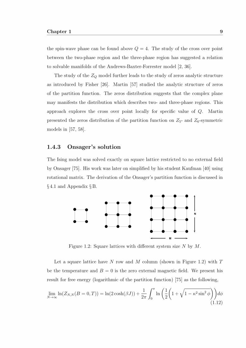
Figure 1.2: Square lattices with different system size N by M .

Let a square lattice have N row and M column (shown in Figure 1.2) with T

be the temperature and B = 0 is the zero external magnetic field. We present his

result for free energy (logarithmic of the partition function) [75] as the following,

limN→∞

ln(ZN,N(B = 0, T )) = ln(2 cosh(βJ)) +1

2π

∫ π

0

ln

(1

2

(1 +

√1− κ2 sin2 φ

))dφ

(1.12)

10 Chapter 1

where κ = 2 sinh(2βJ)/ cosh2(2βJ), β is the inverse temperature and J is the nearest

neighbour interaction strength. ZN,M is the partition function for graph in Figure

1.2.

Other review on the work of Onsager and Kaufman exact solution can also be

found in [6–8, 35, 58].

1.4.4 What can be computed and what it means

The study of model for ferromagnetism aims to investigate the thermodynamic

properties of a physical system [7, 35]. For the Q-state Potts model and for the

three-dimensional lattices, the exact results are still unknown.

Lee and Yang [50, 99] showed that the equation of states of phase transition is

closely related to the root distribution of the partition function. They proved that

under certain conditions the roots always lie on a circle − also known as Lee-Yang

circle theorem. They proposed the concept of zeros in the complex plane to study

the Ising model in magnetic field.

The thermodynamic properties and the phase transition however can only be

explored through the complete distribution of the zeros of the partition function in

the complex-temperature plane. Although only the real value has physical meaning,

the analytic structure of the distribution surprisingly shows a specific behaviour in

the thermodynamic limit [38, 39, 99]. Since the finite lattice partition function is a

positive polynomial, the zeros will always stay off the real axis. The zeros may only

touch the real axis at the thermodynamic limit. We will show the zeros distribution

in details in later chapters.

The study of complex-temperature zeros of partition function for the Ising model

on square lattice in zero magnetic field was first discussed by Fisher [26], and also

by Abe [1], Katsura [38] and Ono and Suzuki [74]. The singularity of specific heat

of the square lattice Ising model is discussed by observing the zeros distribution for

finite lattice size and the endpoints of the arc in the zeros distribution.

The study of statistical mechanical model could be continued further by

Chapter 1 11

investigating the model on different system i.e. different crystal lattice structure

[31, 85] such as triangular, hexagonal and cubic lattices. See § 2.1.2 for detail.

Other study on triangular and hexagonal lattices Potts model can be found for

example in [23, 25, 51, 60, 88, 98].

1.4.5 Phase transition − example of physical phenomena

A phase transition [46, p. 103] occurs when there is a thermodynamic change from

one phase of matter to another phase. One of the study on phase transition is

related to the prediction of critical point for a phase transition − for instance the

Curie temperature [41, 43, 48].

The roots of the partition function are used to study the phase transition and

critical properties in finite size system [29]. The phase transition occurs when the

zeros are distributed in a nice pattern [26] consists of subsets of set of zeros. We

called this a locus of zeros. This locus cut the real axis of the complex plane at the

thermodynamic critical point [87].

The order of phase transition is defined by the behaviour of the derivatives of

free energy [58]. It is called first order transition if there is a discontinuity in the

first derivative of free energy. Similarly, for higher order transition, it is called nth

order if the first discontinuity is at the nth derivative.

For example, consider a graph of specific heat in Figure 1.3. This graph shows

the existence of the second order phase transition. Onsager in his square lattice Ising

model showed that the phase transition was observed when there is a singularity in

the graph of specific heat as shown in this figure.

1.5 Objectives and Aims

We study a model known as Potts model that was introduced by Potts [79]. It

is a generalisation of the Ising model that was introduced by Wilhem Lenz to his

student, Ernst Ising for his doctoral thesis [7, 12, 79]. The case of Ising model

12 Chapter 1

βc

1/k

B C

V

β

Figure 1.3: Specific heat of square lattice Ising model (Onsager’s solution).

on square lattice considered in this thesis serves as a benchmark for checking our

computation. Then we further extend this study to a more general case called the

ZQ-symmetric model.

Our interest is to investigate how macroscopic structure may result from a lower

level activity of a very large number of microscopic structures. The approach in

statistical mechanics can provides prediction when the phase transition of some

material can take place.

The objective is to study the partition functions of these models and their

distribution of zeros of the partition function in the complex plane close to the

phase transition. We aim to investigate the analytic properties of the partition

functions and the relationship between analytic properties and phase transition in

equilibrium statistical mechanics.

In this thesis, we use the transfer matrix [7, 58] approach for computing the

partition function. The partition function is described exactly on the finite lattice

size. The zeros of the partition function are then computed and plotted in the

complex-temperature Argand plane (see the new result of complex-eβ for example

in Figure 1.4).

We study the limiting properties of a physical system by analysing the analytical

behaviour of partition function as the lattice size changes. This is to relate the

Chapter 1 13

-2

-1

0

1

2

-3 -2 -1 0 1 2 3

15x17’

Figure 1.4: 3-state Potts model on 15 by 17 square lattice.

function to the experimental result (see e.g. [7, 35, 101]). With this model, we can

aim to describe physical observable properties for a large system [35, 58].

Outline

The outline of this thesis is as follows. The definitions of Potts model and the

partition function was initially presented in this chapter. This is continued with

the lattice graphs under consideration in Chapter 2. In Chapter 3, the method

of computation of transfer matrix is demonstrated. We show the computation by

simple examples and state the method for finding roots of the partition function.

The results of zeros distribution for the Ising, Q-state Potts and ZQ-symmetric

models will follow in Chapters 4, 5 and 6, respectively. The description of results

starts by considering the solved case of square lattice Ising model in Chapter 4. We

implement the zeros finding approach to the Ising model partition function on square

lattice in this chapter. Chapters 5 and 6 mainly present our investigation for Q-state

Potts and ZQ-symmetric model partition functions and their zeros distributions.

Later, the analysis of the zeros distribution for Ising and Potts models related

14 Chapter 1

to critical exponent of phase transition is presented in Chapter 7. Finally Chapter

8 will discuss the energy-entropy relation and also discuss the possible existence of

multiple phase transitions in ZQ-symmetric models.

Chapter 2

Models on lattice

This chapter describes other details related to Q-state Potts models. The definitions

of the Q-state Potts [3, 20] model was given in § 1.1.

The main object of the study of each model is the partition function. The models

are studied on crystal lattices [64] which will be shown in section § 2.1. Then the

duality relation on partition function will be introduced.

The modern technology like the X-ray crystallography facility [52, 85, 91, 100]

allows us to see the lattice feature in solid state material. For example, the

lattice arrangement in aluminium and magnesium is given by face-centered cubic

and hexagonal close-packed respectively. This lattice arrangement is following the

classification of lattice system described in the field of crystallography [11, 18, 82, 97].

2.1 Graph of regular lattice

This section will describe the lattice graphs under consideration in this thesis. The

aim is to compute a partition function Z for a specific lattice graph Λ representing

a laboratory size piece of crystal structure. Unfortunately, due to limitation of

computing resources, we are not able to compute the Z on very large lattice size. So

instead, we consider a sequence of finite lattices which in suitable sense (see § 4.3)

extends to contain the laboratory sample.

15

16 Chapter 2

2.1.1 Thermodynamic limit

The lattice graph is studied based on the motivation from physics. We consider a

sequence of finite lattice graphs arranged in increasing lattice sizes. Although the

result of physical observable is affected by the finite size effect (explain in § 4.3), at

large enough size, some kinds of observation reach stability. The size dependence

will vanish in a good model, since the bulk observables of a physical system do not

depend strongly on lattice size in the laboratory [87, p. 69].

The study of statistical mechanics aims to predict the bulk behaviour for a

physical system i.e. behaviour which is independent from the size of the system.

In particular, a sequence of lattices all approaching a ‘limit’ lattice in a way that

captures stable limiting behaviour is needed for the study. This sequence of lattices

consists of many lattices of the same type but in different sizes (such as square

lattices in Figure 2.2). Although the exact such sequence is not prescribed, from the

Onsager’s solution [40, 75], we know that the sequence of square lattices does have

a stable limit (thermodynamic limit [35, 58]) for suitable observables.

Given these requirements, we define a sequence of lattices which includes

computable cases and laboratory size cases. Our hope is that limiting behaviour

is already observed in the computable cases. Here, we describe only the first step

i.e. defining the sequence.

2.1.2 Lattice graph

Here the specific sequence of graphs for each Hamiltonian will be presented. In two-

dimensional case, the regular patterns under consideration are the square, triangle

and hexagon. In three-dimensional case, the patterns under consideration are the

cubic, tetrahedron and octahedron. In literature what we refer to as the hexagonal

pattern is often referred to as the honeycomb lattice.

In crystallography, the crystal structure is described in two ways [85, p. 60].

First they are based on seven basic geometry shapes of unit cell in three-dimensional

Chapter 2 17

space. This type of shape is called the seven crystal systems. The second is related

to the way in which atoms are arranged in a unit cell. The unit cell is the smallest

structure in three-dimensional space which translated itself to form the whole crystal.

This atomic arrangement is called the Bravais lattice [31, 48, 85]. The repetition of

regular lattice shape is the nearest approximation towards many real structure of

crystalline materials.

2.1.2.1 d-dimensional lattice

The lattice graph is constructed under a graph embedding to d-dimensional

Euclidean space Rd [32] consist of a finite set of regularly spaced sites. The vertex

of the graph is associated to the lattice site and the edge of the graph represents the

nearest neighbour interaction between vertices.

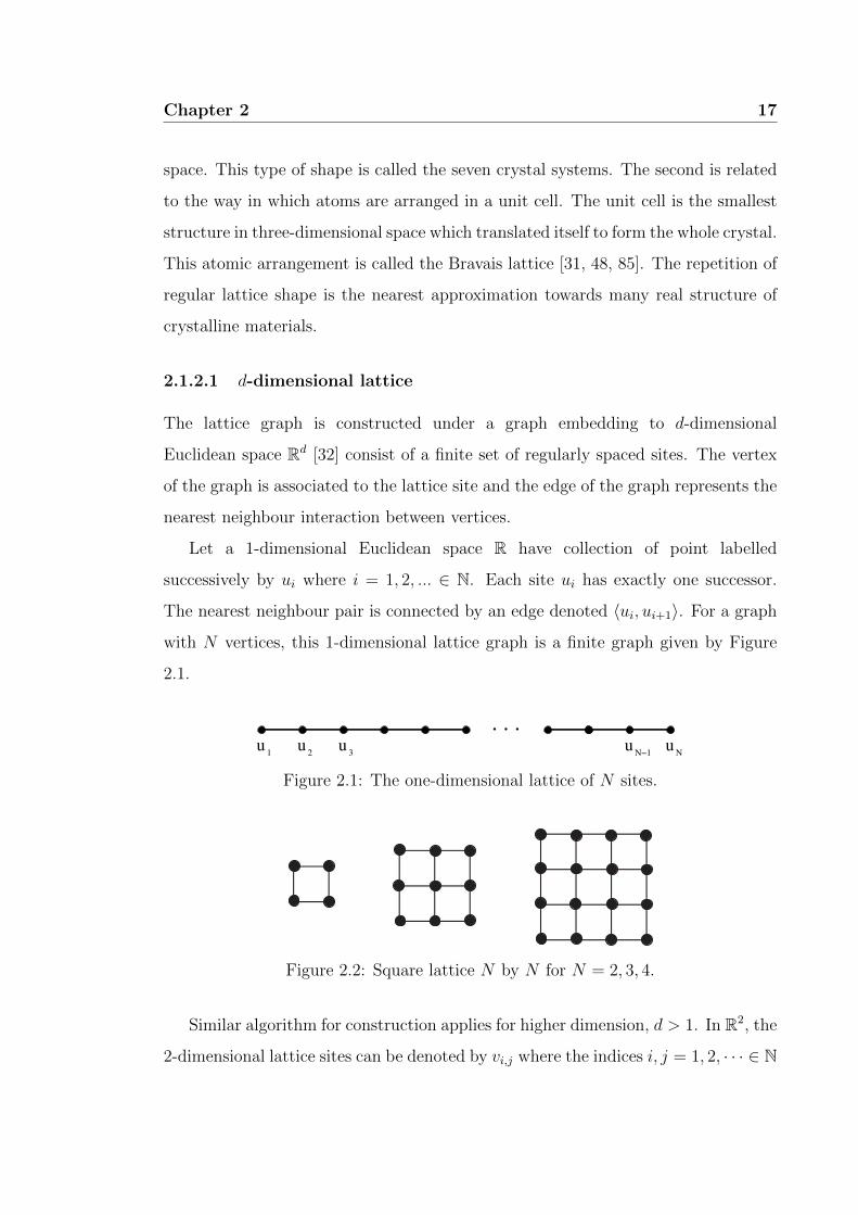
Let a 1-dimensional Euclidean space R have collection of point labelled

successively by ui where i = 1, 2, ... ∈ N. Each site ui has exactly one successor.

The nearest neighbour pair is connected by an edge denoted 〈ui, ui+1〉. For a graph

with N vertices, this 1-dimensional lattice graph is a finite graph given by Figure

2.1.

. . .

u1 3

uu2

uN

uN−1

Figure 2.1: The one-dimensional lattice of N sites.

Figure 2.2: Square lattice N by N for N = 2, 3, 4.

Similar algorithm for construction applies for higher dimension, d > 1. In R2, the

2-dimensional lattice sites can be denoted by vi,j where the indices i, j = 1, 2, · · · ∈ N

18 Chapter 2

correspond to the row vertices i and the column vertices j.

Let each lattice site vi,j have two successive nearest neighbours that are at i+ 1

given j and j + 1 given i. The nearest neighbour pairs are denoted by 〈vi,j, vi+1,j〉

and 〈vi,j, vi,j+1〉. For N row and M column vertices, the graph forms N by M square

lattice structure shown in Figure 2.2. We shall denote the d-dimensional lattice by

N1 ×N2 × · · · ×Nd for all number of vertices in respective directions, Ni ∈ N.

A triangular lattice in contrary has three successive nearest neighbours at each

lattice site. The nearest neighbours are given by pairs 〈vi,j, vi+1,j〉, 〈vi,j, vi,j+1〉 and

〈vi,j, vi+1,j+1〉.

The hexagonal lattice in addition is constructed as follows. For i, j = 1, 2, · · · ∈

N, if i is odd, the sites will have one successive neighbour, 〈vi,j, vi,j+1〉 when j is

even and two successive neighbours, 〈vi,j, vi,j+1〉 and 〈vi,j, vi+1,j〉 when j is odd.

Conversely if i is even, the sites will have two successive neighbours, 〈vi,j, vi,j+1〉

and 〈vi,j, vi+1,j〉 when j is even and one successive neighbour 〈vi,j, vi,j+1〉 when j is

odd. See illustration in Figure 2.4. For computer program, we can drop the hexagon

shape and compute the partition function by layering the lattice into a rectangular

shape.

Figure 2.3: Triangular lattice.

2.1.2.2 Dense sphere packing

In this thesis we consider two types of dense sphere packing which are the face-

centered cubic (fcc) and the hexagonal close packing (hcp).

The face-centered cubic packing is obtained from a simple cubic geometry. At

each vertex point of a cubic lattice, there exist one spin variable and for each face

of the cubic, there exist another spin variable. Each vertex point is assumed to be

Chapter 2 19

Figure 2.4: Hexagonal lattice (left) to rectangular graph layering (right) forcomputer program.

Figure 2.5: Cubic lattice.

Figure 2.6: Octagonal lattice i.e. face-centered cubic lattice.

Figure 2.7: Tetragonal lattice i.e. hexagonal close-packed lattice.

20 Chapter 2

a sphere of radius 1. See Figure 2.8. The cubic shape is the unit cell of the lattice.

The dash lines correspond to edges in the lattice graph.

The length of each edge of the cube is√

8 and the diagonal distance of each face

is 4. In total, there are 4 spheres in the cubic unit cell of this face-centered cubic

lattice.

A crystal lattice has dense sphere packing if it has highest number of atomic

density in a unit cell. The number of atomic density is also called the atomic

packing factor representing the fraction of volume occupied by atoms in a unit cell

over the volume of the same unit cell [85] i.e.

4π(43)

(√

8)3=

π√18.

Figure 2.8: Structure showing the face-centered cubic lattice point arrangement ina unit cell.

Likewise, the case of hexagonal close packing has the same density packing i.e.π√18

. Their unit cells are occupied by the same number of atoms that is 12 atoms

but are different by their packing sequence.

The packing construction is described based on the pattern of each layer of the

lattice. See Figure 2.9 for illustration. For the face-centered cubic, the packing

structure follows the successive layer with ABC sequence whereas the packing

sequence for the hexagonal close-packed follows the AB pattern. The overline

notation such as in the AB pattern means the repetition of atomic packing sequence

in each lattice layer (first layer in position A, then second layer in position B, then

repeat the position back to A and B and so on). More detailed explanation can be

found in the book by Shackelford [85] and Hales [31].

Chapter 2 21

We describe the dense sphere packing by the illustration of repeated polyhedra

glued together forming a finite three-dimensional lattice. This choice assists the

computation of the transfer matrix which will be explained in the next chapter. We

call the face-centered cubic and the hexagonal close-packed as the octagonal and

tetragonal lattices respectively.

A

AA

AA

A

A

B

B

B

C

CC

(a) ABC stacking sequence.

Normal to close−packed plane

C

B

A

A

Close−packed planes

(b) Face-centered cubic.

A

AA

AA

A

A

B

B

B

(c) AB stacking sequence.

Close−packed planes

A

B

A

Normal to close−packed planes

(d) Hexagonal close-packed.

Figure 2.9: Face-centered cubic, hexagonal close-packed and their stacking sequencerespectively.

2.1.3 Boundary condition

Consider a finite cubic lattice Nx × Ny × Nz embedded in R3. The rest of the R3

space is left empty (vacuum). The condition separating the vacuum space from the

filled spaced is called the boundary condition. We call the outer sites of the lattice

22 Chapter 2

as the boundary sites or exterior sites. The inner sites are called interior sites (see

Figure 2.11). In general, each lattice site has 2d nearest neighbours except at the

boundary [17].

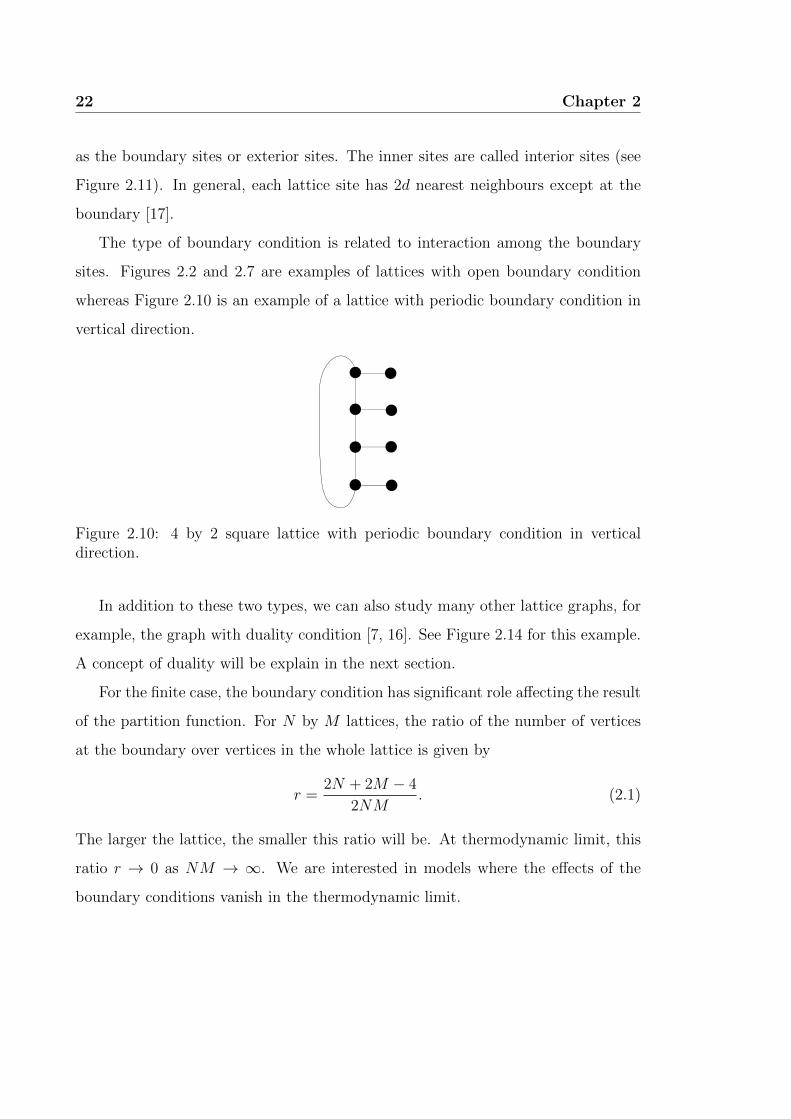
The type of boundary condition is related to interaction among the boundary

sites. Figures 2.2 and 2.7 are examples of lattices with open boundary condition

whereas Figure 2.10 is an example of a lattice with periodic boundary condition in

vertical direction.

Figure 2.10: 4 by 2 square lattice with periodic boundary condition in verticaldirection.

In addition to these two types, we can also study many other lattice graphs, for

example, the graph with duality condition [7, 16]. See Figure 2.14 for this example.

A concept of duality will be explain in the next section.

For the finite case, the boundary condition has significant role affecting the result

of the partition function. For N by M lattices, the ratio of the number of vertices

at the boundary over vertices in the whole lattice is given by

r =2N + 2M − 4

2NM. (2.1)

The larger the lattice, the smaller this ratio will be. At thermodynamic limit, this

ratio r → 0 as NM → ∞. We are interested in models where the effects of the

boundary conditions vanish in the thermodynamic limit.

Chapter 2 23

Figure 2.11: Increasing sizes of square lattices. The red sites highlight the spins atboundary and the black sites are the interior sites.

2.2 Duality

In this section, the concept of duality transformation [83] will be introduced.

Let G = (V,E, f) be a graph defined as in § 1.1.

Definition 2.2.1 ([95]). A curve is the image of a continuous map from [0, 1] to

R3. A polygonal curve is a curve composed of finitely many line segments. It is a

polygonal u, v−curve when it starts at u and ends at v. It has no self crossing with

individual polygonal curve.

Definition 2.2.2 ([95]). A drawing of a graph G is a function f defined on V ∪ E

that assigns each vertex v a point f(v) in the plane and assigns each edge with

endpoints u, v a polygonal f(u), f(v)−curve i.e. f : V → R3 and f : E → f(E).

The images of vertices are distinct. A point in f(e) ∩ f(e′) that is not a common

endpoints is a crossing. The curve cannot have a changing direction at the crossing

point.

Definition 2.2.3 ([95]). Let G = (V,E, f) be a graph. The graph G is planar if it

has a drawing f without crossings. Such drawing is a planar embedding of G. A

plane graph is a particular planar embedding of a planar graph.

For any planar graph G, we can form a related plane graph called its dual. Here

we introduce a notion of face F . A face is a region bounded by edges including the

24 Chapter 2

outer infinite region. Let FG be the set of faces in G.

Suppose G∗ = (V ∗, E∗, f ∗) be another planar graph that is a dual to G. The

graph G∗ has the following construction. The set of vertices v∗ ∈ V ∗ corresponds to

the face Fi ∈ FG. For each e ∈ E with face Fi on one side and Fj on another side,

the endpoint of edge e∗ ∈ E∗ are the vertices v∗, w∗ ∈ V ∗ that represent the faces

Fi, Fj of G.

Now, we introduce a notion of a body that is region bounded by faces, separating

its inner and outer regions.

Let L = (V,E, f) be a graph defined as in § 1.1. A graph L embedded in

Euclidean space R3 is a 1-to-1 function φ1 : V → R3 and a continuous function

φ2 :

[0,1]e⋃e∈E

→ R3 that is also 1-to-1 on

[0,1]e⋃e∈E

such that φ2(0), φ2(1) = φ(f(e)). The

[0, 1]e corresponds to the edge in the graph. The embedding of graph L has also a

1-to-1 function φ3 :

([0,1]×[0,1])p⋃p∈FL

→ R3. The ([0, 1]× [0, 1])p corresponds to the face of

the graph L.

Consider for example, the embedding for a cubic graph L = (V,E, f). The

body of a cubic is bounded by square faces p ∈ FL. Let L∗ = (V ∗, E∗, f ∗) be the

dual graph of L. The graph L∗ has the following construction. The vertex of L

corresponds to the body of L∗. The edge of L is then corresponds to the face of

L∗. Also the face of L corresponds to the edge of L∗ which is perpendicular to the

surface of the face L. Finally the body of L corresponds to the point of L∗ which

located in the center of the cubic L. The dual graph for a cubic graph is again a

cubic graph.

Figure 2.12 present the illustration of a square lattice and its dual, which is a

self-dual up to boundary condition. Figure 2.13 in addition manifests the graph of

hexagonal lattice and its dual graph i.e. the triangular lattice. The case shown in

Figure 2.14 has been studied by Chen, Hu and Wu [16].

A dual of a model is a mapping of a model to another model. For example, a

dual of a 2-dimensional Ising model using a certain transformation, could be exactly

Chapter 2 25

Figure 2.12: Square lattice and its dual.

rewritten as another 2-dimensional Ising model [42, 83]. The high-temperature

regions of the original Ising model is mapped to the low-temperature regions of its

dual, and vice versa. This is a self-dual model which had been showed by Kramers

and Wannier [44].

Figure 2.13: Hexagonal lattice and its dual, a triangular lattice.

The duality transformation on lattice model is a useful tool for passing

information of one model to its dual. The duality relation for 2-dimensional Q-

state Potts model will be given in § 2.2.2.

2.2.1 Z in dichromatic polynomial

Here we derive the partition function in a dichromatic polynomial form. We rewrite

the partition function which will allow us to express the duality relation in the

partition function. It relates the graph G and its dual graph G∗.

26 Chapter 2

Figure 2.14: Self-dual square lattice.

With some modification, the partition function can be written in terms of graph

G and its subgraph. Let G′ ⊆ G, VG′ = V and EG′ ⊆ E. Recall x = eβJ . For

simplicity, let the interaction strength J = 1 and introduce a new variable v = x−1.

For writing purposes, we write σ(j) as σj for any j ∈ N.

The partition function (1.1) for Q-state Potts model can be written in terms of

v,

ZG =∑σ∈Ω

exp(−βH(σ))

=∑σ∈Ω

exp(βJ∑


δσiσj)

=∑σ∈Ω

∏〈i,j〉=f(e),

e∈E

exp(βδσiσj)

=∑σ∈Ω

∏〈i,j〉=f(e),

e∈E

(1 + vδσiσj) (2.2)

where

(1 + vδσiσj) =

1, if σi 6= σj

x, if σi = σj

.

The expansion of this relation will express Z in terms of a dichromatic polynomial

[5, 56, 58]. One of the possible ways to describe the equation (2.2) is by considering

a power set.

Chapter 2 27

Definition 2.2.4. Given a set A, the power set P of A is the set of all subsets of

A.

Alternatively, we call the edge in the graph a bond. Let P be the power set of

the set of bonds in E to Z2 = 0, 1, i.e. P : E → Z2. Then

ZG =∑σ∈Ω

∏〈i,j〉=f(e),

e∈E

(1 + vδσiσj)

=∑σ∈Ω

∑EG′∈P(E)

v|EG′ |∏

〈i,j〉=f(e),e∈EG′

(δσiσj). (2.3)

The first summation is over all possible configuration of Ω. The second

summation is over the elements of the power set P of the set of edges. See illustration

in Figure 2.15. The EG′ can be illustrated by bond denoted with 0 and 1; respectively

corresponds to missing bond and filled bond. We call this a bond covering 0 and 1

respectively.

(a)

(b)

Figure 2.15: Set of bonds EG′ can be illustrated by bond 0 and 1.

The expression v|EG′ |∏

〈i,j〉=f(e),e∈EG′

(δσiσj) is forced to zero for every configuration

summation which all the spins connected by filled bonds that are not aligned.

Then the dichromatic polynomial is as the following:

ZG =∑G′⊆G

v|EG′ |Q|C(G′)| (2.4)

28 Chapter 2

where |C(G′)| = c is the number of connected clusters in G′, including isolated

vertices. The connected cluster refer to the isolated sublattice with vertices

connected by one or more edges and also the individual vertex (with no edge).

The value of Qc is the total number of configurations in which the filled bonds

form c connected clusters. Refer illustration below for examples.

a) b)

Figure 2.16: Example of connected cluster including its isolated vertices witha)|C(G′)| = 4 and b)|C(G′)| = 3.

For the 2-state Potts model, let |E| = L be the total number of edges and

|V | = N be the number of vertices. Again by equation (2.2) we take

ZG =∑σ∈Ω

∏〈i,j〉=f(e),

e∈E

(1 + vδσiσj)

=∑σ∈Ω

∏〈i,j〉=f(e),

e∈E

(1 + (eβ − 1)δσiσj)

=∑σ∈Ω

∏〈i,j〉=f(e),

e∈E

(eβ + 1

2+eβ − 1

2(2δσiσj − 1)

). (2.5)

Alternatively, the bond coverings mentioned earlier may be reinterpreted

corresponding to the possible choices of the new summation in the expansion of

the product in equation (2.5). A bond covering corresponds to the number of edges

at each vertex. The lattice graph has even bond covering if each vertex of the

subgraph G′ has even number of edges.

Chapter 2 29

Factor out the largest term of the product,

ZG =∑σ∈Ω

∑EG′∈P(E)

(x+ 1

2

)L−|EG′ |(x− 1

2

)|EG′ | ∏〈i,j〉=f(e),e∈EG′

(2δσiσj − 1)

=

(x+ 1

2

)L∑σ∈Ω

∑EG′∈P(E)

(x− 1

x+ 1

)|EG′ | ∏〈i,j〉=f(e),e∈EG′

(2δσiσj − 1). (2.6)

(a) (b)

Figure 2.17: Examples of non-even bond covering.

Example 2.2.1. Given a graphG with open boundary condition. For the expression∑σ∈Ω

∏〈i,j〉=f(e),e∈EG′

(2δσiσj − 1) the individual case shown in Figure 2.17a and 2.17b have

value ∑σ∈Ω

(2δσ1σ2 − 1) = 0∑σ∈Ω

(2δσ1σ2 − 1)(2δσ2σ3 − 1) = 0.

respectively.

The expression∑σ∈Ω


(2δσiσj − 1) always equal to 0 when the subgraph G′

30 Chapter 2

describes the non-even covering of G; i.e.∑σ∈Ω


(2δσiσj − 1) =∑σ∈Ω

(2δσiσj − 1)

=∑σ∈Ω

2δσiσj −∑σ∈Ω

1

= 2∑σ∈Ω

δσiσj − 2N

= 2.2N−1 − 2N

= 0. (2.7)

Thus we have,

Z =

(x+ 1

2

)L2N

∑EG′∈P(E),

even covering G′

(x− 1

x+ 1

)|EG′ |

=

(x+ 1

2

)L2N

∑even covering

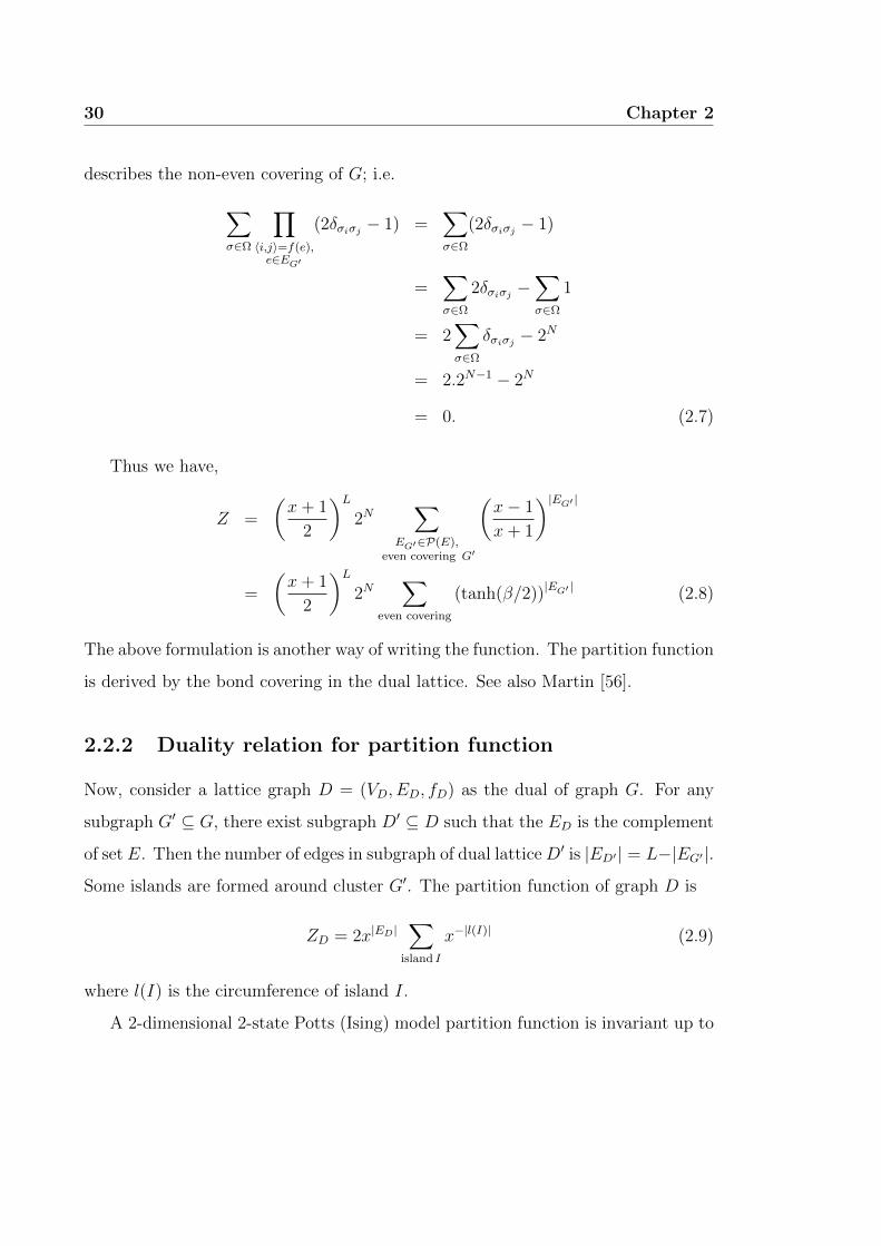
(tanh(β/2))|EG′ | (2.8)

The above formulation is another way of writing the function. The partition function

is derived by the bond covering in the dual lattice. See also Martin [56].

2.2.2 Duality relation for partition function

Now, consider a lattice graph D = (VD, ED, fD) as the dual of graph G. For any

subgraph G′ ⊆ G, there exist subgraph D′ ⊆ D such that the ED is the complement

of set E. Then the number of edges in subgraph of dual latticeD′ is |ED′| = L−|EG′|.

Some islands are formed around cluster G′. The partition function of graph D is

ZD = 2x|ED|∑

island I

x−|l(I)| (2.9)

where l(I) is the circumference of island I.

A 2-dimensional 2-state Potts (Ising) model partition function is invariant up to

Chapter 2 31

the boundary condition under this transformation [58, §1.5]

x−1 ↔ x− 1

x+ 1. (2.10)

For arbitrary value of spin state Q, the duality has the following relation:

x↔ x+ (Q− 1)

x− 1. (2.11)

A model on a square lattice is one simple example of this duality. It has the

self-duality properties which holds up to the boundary.

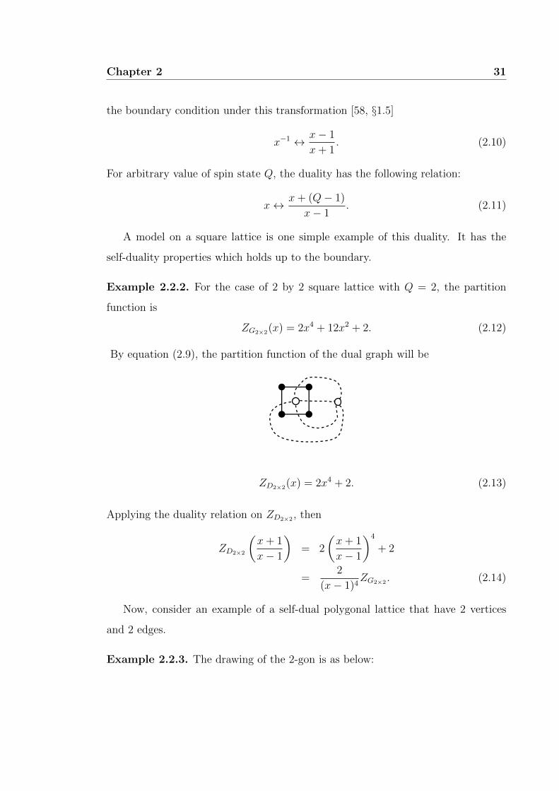
Example 2.2.2. For the case of 2 by 2 square lattice with Q = 2, the partition

function is

ZG2×2(x) = 2x4 + 12x2 + 2. (2.12)

By equation (2.9), the partition function of the dual graph will be

ZD2×2(x) = 2x4 + 2. (2.13)

Applying the duality relation on ZD2×2 , then

ZD2×2

(x+ 1

x− 1

)= 2

(x+ 1

x− 1

)4

+ 2

=2

(x− 1)4ZG2×2 . (2.14)

Now, consider an example of a self-dual polygonal lattice that have 2 vertices

and 2 edges.

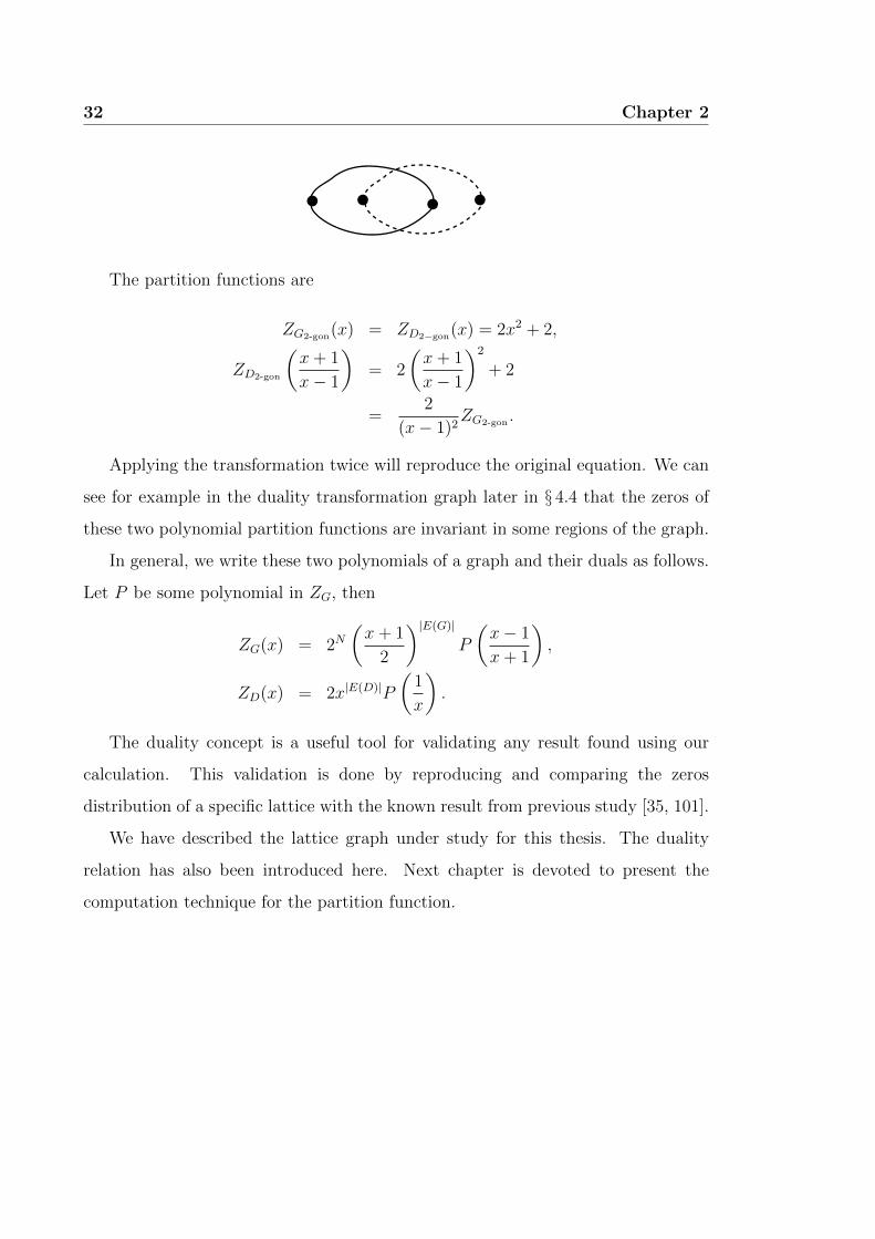
Example 2.2.3. The drawing of the 2-gon is as below:

32 Chapter 2

The partition functions are

ZG2-gon(x) = ZD2−gon(x) = 2x2 + 2,

ZD2-gon

(x+ 1

x− 1

)= 2

(x+ 1

x− 1

)2

+ 2

=2

(x− 1)2ZG2-gon .

Applying the transformation twice will reproduce the original equation. We can

see for example in the duality transformation graph later in § 4.4 that the zeros of

these two polynomial partition functions are invariant in some regions of the graph.

In general, we write these two polynomials of a graph and their duals as follows.

Let P be some polynomial in ZG, then

ZG(x) = 2N(x+ 1

2

)|E(G)|

P

(x− 1

x+ 1

),

ZD(x) = 2x|E(D)|P

(1

x

).

The duality concept is a useful tool for validating any result found using our

calculation. This validation is done by reproducing and comparing the zeros

distribution of a specific lattice with the known result from previous study [35, 101].

We have described the lattice graph under study for this thesis. The duality

relation has also been introduced here. Next chapter is devoted to present the

computation technique for the partition function.

Chapter 3

Computation for partition

function

In this chapter we present the computation of a transfer matrix [7, 58] for

the partition function on finite lattice. We begin with an example of model

configurations on lattice in the first section. Then it is followed by the description

of the partition vector and transfer matrix. The final section will briefly stated the

zeros finding for the partition function.

Initially a brute-force approach [81] is used for computation where the

Hamiltonian is directly substituted into the partition function (1.1). This approach

requires long period of time and requires many calculations as the lattice size

increases. The number of configuration states increases exponentially with respect

to number of vertices on graph.

For this reason, a better approach is needed to reduce the number of calculations

for the partition function. For that we use a transfer matrix approach.

3.1 Models on lattice − example

In this chapter, we consider the Q-state Potts model on a square lattice. Let a

square lattice have discrete variables called vertices with associated spin which can

33

34 Chapter 3

take any value Q = 1, 2, ..., Q representing the spin directions.

Recall Definition 1.1.1 of a graph. Let Γ = (V,E, f) be a square lattice graph.

Then |V | is the number of vertices in the lattice. The total number of configuration

states is given by |Ω| = Q|V |. The state σ = σi|i is indexed for location of the

spin ∈ Ω. Each spin variable interacts with its nearest neighbours will gives value

1 if the pair spins in the same direction and 0 otherwise.

Figure 3.1 shows all possible microstates for 2 by 2 square lattice. The spin

up denoted as ‘+’ and down as ‘−’ correspond to spin 1 and 2 respectively. For a

2-state Potts model on 2 by 2 square lattice, Ω is given by

Ω = (1, 1, 1, 1), (1, 1, 1, 2), (1, 1, 2, 1), (1, 1, 2, 2),

(1, 2, 1, 1), (1, 2, 1, 2), (1, 2, 2, 1), (1, 2, 2, 2),

(2, 1, 1, 1), (2, 1, 1, 2), (2, 1, 2, 1), (2, 1, 2, 2),

(2, 2, 1, 1), (2, 2, 1, 2), (2, 2, 2, 1), (2, 2, 2, 2) (3.1)

|Ω| = 24 = 16 .

1

2

3

4

σ

σ

σ

σ

(a)

+ +

++

+ +

+

+

++

+

+

+ +

+

+ + +

+

+

+

++

+

+ ++ +

+

+

+

+

_

_ _

_

_

_

_

_

_

_

_

_

__

_

__

_ _ _ _

_

_

_ _

_ _

_

_

_ _

_

(b)

Figure 3.1: 2 by 2 square lattices.

Recall Definition 1.1.5 of the Q-state Potts model Hamiltonian. For any σ(i) =

Chapter 3 35

(σ1, σ2, σ3, σ4) ∈ Ω, if σ(1) = (1, 1, 1, 1) and σ(2) = (1, 2, 1, 2), we have Hamiltonian

H(σ(1)) = −J(δσ1σ2 + δσ2σ4 + δσ1σ3 + δσ3σ4)

= −J(1 + 1 + 1 + 1) = −4J

and

H(σ(2)) = −J(δσ1σ2 + δσ2σ4 + δσ1σ3 + δσ3σ4)

= −J(0 + 1 + 1 + 0) = −2J.

Computing the Hamiltonian for all its microstates and x = eβJ gives partition

function

Z = 2e4βJ + 12e2βJ + 2

= 2x4 + 12x2 + 2.

This is the result we see in equation (2.12).

3.2 Partition Vector and Transfer Matrix

This section will describe the approach used to expedite the computation of the

partition function. For this purpose, we use the partition vector and transfer matrix

approach.

The Hamiltonian information on the lattice model is arranged into a vector in the

space of all configurations of the boundary spin variables. We call this a partition

vector. We describe in details as follows.

For any lattice graph, we denote c as the set of all exterior sites. The set

of microstate of graph G is denoted ΩG. Let VG be all vertices in a graph G.

The V ′ ⊆ VG is the set of exterior on the graph with set of state ΩV ′ . Denote

σB ∈ ΩV ′ as the spin configurations at boundary. A set of microstates given fixed

spin configurations at boundary is denoted as ΩVG |σB ⊂ ΩG.

36 Chapter 3

Example 3.2.1. Let Γ = (VΓ, EΓ, f) be a graph of 2 by 2 square lattice for 2-states

Potts model shown in Figure 3.1. Denote VΓ = σ1, σ2, σ3, σ4 and V ′ = σ3, σ4 ⊂

VΓ. The set of all configuration states ΩΓ is given by (3.1). Let spin configurations

at boundary given by ΩV ′ , i.e.

ΩV ′ = (1, 1), (1, 2), (2, 1), (2, 2).

So if σB1 = (1, 1) and σB2 = (2, 1), we have

ΩΓ|(1,1) = (1, 1, 1, 1), (1, 2, 1, 1), (2, 1, 1, 1), (2, 2, 1, 1)

ΩΓ|(2,1) = (1, 1, 2, 1), (1, 2, 2, 1), (2, 1, 2, 1), (2, 2, 2, 1).

The partition function with the fixed spin configurations at σB is given by

ZV ′

Γ |σB :=∑

σ∈ΩΓ|σB

exp(−βH(σ)).

Definition 3.2.1. The partition vector ZV ′

G is the vector arrangement in space of

all fixed boundary or exterior sites of a lattice system. For σB ∈ ΩV ′, we have

ZV ′

G = ZV ′

G |σ1 , ZV ′

G |σ2 , ....

The full partition function is then defined as

ZG =∑

σB∈ΩV ′

ZV ′

G |σB . (3.2)

This vector arrangement can produce a partition function for two combined

lattice graphs. A bigger lattice can be formed by combining two lattices through a

vector multiplication.

Definition 3.2.2. Let G,G′ be two lattice graphs. For the union of two graphs

G ∪G′ we have

VG∪G′ = VG ∪ VG′

EG∪G′ = EG ∪ EG′ .

Chapter 3 37

The E is the set of edges and EG ∩ EG′ = ∅.

The partition function of the new graph GG′ is given by a summation of the

product of partition vectors for graph G and G′ (as in Definition 3.2.1). This is

given by

ZGG′ =∑σ∈ΩV ′

(ZV ′

G |σ)(ZV ′

G′ |σ). (3.3)

This equation is given by the Chapman-Kolmogorov theorem [76]. See Figure 3.3

for example of a combined graph.

Theorem 3.2.1 (Chapman-Kolmogorov [76]). Let G and G′ be graphs such that

EG ∩ EG′ = ∅. Let GG′ denote G ∪G′ and V ′ = VG ∩ VG′. Then

ZGG′ =∑σ∈ΩV ′

(ZV ′

G |σ)(ZV ′

G′ |σ) = ZV ′

G ZV ′

G′ . (3.4)

Proof. Recall partition function (1.1). For graph GG′ = G ∪G′, we have

ZGG′ =∑

σ∈ΩVGG′

exp(βHGG′(σ)). (3.5)

For EG ∩ EG′ = ∅ and σ ∈ ΩVGG′,

HGG′(σ) = HG(σ) +HG′(σ).

For V ′ = VG ∩ VG′ , we have

ZGG′ =∑

σ∈ΩVGG′

(exp(βHG(σ))) (exp(βHG′(σ)))

=∑σ∈ΩV

∑σ∈ΩVG|σ

exp(βHG(σ))

∑σ∈ΩVG′ |σ

exp(βHG′(σ))

=

∑σ∈ΩV

(ZV ′

G |σ) (

ZV ′

G′ |σ). (3.6)

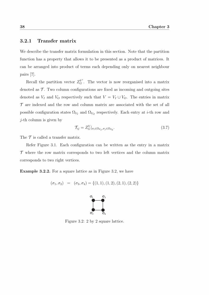
38 Chapter 3

3.2.1 Transfer matrix

We describe the transfer matrix formulation in this section. Note that the partition

function has a property that allows it to be presented as a product of matrices. It

can be arranged into product of terms each depending only on nearest neighbour

pairs [7].

Recall the partition vector ZV ′

G . The vector is now reorganised into a matrix

denoted as T . Two column configurations are fixed as incoming and outgoing sites

denoted as VI and VO respectively such that V = VI ∪ VO. The entries in matrix

T are indexed and the row and column matrix are associated with the set of all

possible configuration states ΩVI and ΩVO respectively. Each entry at i-th row and

j-th column is given by

Tij = ZVG |σi∈ΩVI ,σj∈ΩV0

. (3.7)

The T is called a transfer matrix.

Refer Figure 3.1. Each configuration can be written as the entry in a matrix

T where the row matrix corresponds to two left vertices and the column matrix

corresponds to two right vertices.

Example 3.2.2. For a square lattice as in Figure 3.2, we have

(σ1, σ2) = (σ3, σ4) = (1, 1), (1, 2), (2, 1), (2, 2)

1

2

3

4

σ

σ

σ

σ

Figure 3.2: 2 by 2 square lattice.

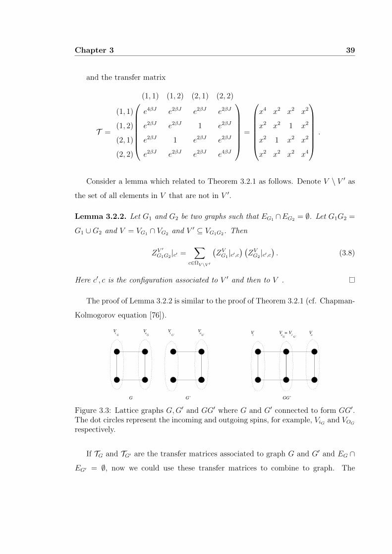
Chapter 3 39

and the transfer matrix

T =

(1, 1) (1, 2) (2, 1) (2, 2)

(1, 1) e4βJ e2βJ e2βJ e2βJ

(1, 2) e2βJ e2βJ 1 e2βJ

(2, 1) e2βJ 1 e2βJ e2βJ

(2, 2) e2βJ e2βJ e2βJ e4βJ

=

x4 x2 x2 x2

x2 x2 1 x2

x2 1 x2 x2

x2 x2 x2 x4

.

Consider a lemma which related to Theorem 3.2.1 as follows. Denote V \ V ′ as

the set of all elements in V that are not in V ′.

Lemma 3.2.2. Let G1 and G2 be two graphs such that EG1 ∩EG2 = ∅. Let G1G2 =

G1 ∪G2 and V = VG1 ∩ VG2 and V ′ ⊆ VG1G2. Then

ZV ′

G1G2|c′ =

∑c∈ΩV \V ′

(ZVG1|c′,c) (ZVG2|c′,c). (3.8)

Here c′, c is the configuration associated to V ′ and then to V .

The proof of Lemma 3.2.2 is similar to the proof of Theorem 3.2.1 (cf. Chapman-

Kolmogorov equation [76]).

G’ GG’G

V V VVV = V

Vo

oo

oi

ii

VGG

iG’ G’

G’G

Figure 3.3: Lattice graphs G,G′ and GG′ where G and G′ connected to form GG′.The dot circles represent the incoming and outgoing spins, for example, ViG and VOGrespectively.

If TG and TG′ are the transfer matrices associated to graph G and G′ and EG ∩

EG′ = ∅, now we could use these transfer matrices to combine to graph. The

40 Chapter 3

incoming and outgoing spins are denoted as ViG and VOG respectively for graph G

and ViG′ and VOG′ respectively for graph G′.

Similar to partition vector multiplication, we can now combine two graphs by a

matrix multiplication. By equation (3.7) and Lemma 3.2.2, the transfer matrix of

two combined graph is given by matrix product

TGG′ = TG TG′

where ViGG′ = ViG and VOGG′ = VOG′ .

The partition function of the new graph is given by

ZGG′ =d∑i=1

d∑j=1

(TGG′)i,j (3.9)

where i, j is the index of matrix TGG′ and d is the dimension of the matrix.

This combining process is restricted to the incoming and outgoing spins. Once

combined the outgoing spins of G and incoming spins of G′ become the interior spin

variables of graph GG′, or VOG = ViG′ .

Example 3.2.3. Let graph G ∪ G′ given by Figure 3.3. The transfer matrices of

individual graph are given by TG and TG′ , i.e.

TG =

x4 x2 x2 x2

x2 x2 1 x2

x2 1 x2 x2

x2 x2 x2 x4

and TG′ =

x3 x x x

x2 x2 1 x2

x2 1 x2 x2

x x x x3

.

A combination of graph G and G′

gives

TGG′ = TG TG′

=

x7 + 2x4 + x3 x5 + x4 + x3 + x2 x5 + x4 + x3 + x2 2x5 + 2x4

x5 + x4 + x3 + x2 x4 + 2x3 + 1 2x3 + 2x2 x5 + x4 + x3 + x2

x5 + x4 + x3 + x2 2x3 + 2x2 x4 + 2x3 + 1 x5 + x4 + x3 + x2

2x5 + 2x4 x5 + x4 + x3 + x2 x5 + x4 + x3 + x2 x7 + 2x4 + x3

.

Chapter 3 41

And finally the partition function for GG′ is given by

ZGG′ = 2x7 + 12x5 + 18x4 + 18x3 + 12x2 + 2.

3.2.2 Boundary Condition

Here we present two types of boundary condition that we consider in this thesis.

The boundary conditions are called open and periodic boundary conditions (we refer

to § 2.1.3 and also [58]).

We say a lattice has an open boundary condition when there is no connecting

edge between two exterior vertices. Otherwise, it is a periodic boundary condition.

u u'

Figure 3.4: 5 by 5 square lattice with periodic boundary in vertical direction.

Figure 3.4 shows a 5 by 5 square lattice with both types of boundary condition.

The grey coloured particles correspond to the exterior sites of the lattice. The

disconnected dashed lines correspond to edges connecting the first and the lowest

rows whereas there is no edge connecting the first and the last column. The latter

shows an open boundary condition in horizontal direction and the former refers to

the periodicity in vertical direction. We had assumed an open boundary condition

for all previous examples.

For N,M ∈ N, let N by M be the size of any square lattice graph Γ with N row

and M column vertices. Let T be the transfer matrix. The partition function for

42 Chapter 3

lattices with open horizontal boundary conditions is defined as [58].

Zopen =∑ij

(T M)ij (3.10)

The partition function for a lattice with periodic boundary condition in all directions

eventually becomes a trace of the matrix.

Zperiodic =∑ii

(T M)ii = tr(T M). (3.11)

3.2.3 Symmetry on graph

Here we present some available symmetries in some lattices which will further speed

up the calculation for partition function [58].

The implementation of the symmetries in the computation is as follows. We

classify all the configurations σ ∈ Ω into some subsets of Ω. We call them a symmetry

class where its elements are the result of the translation, spin, reflection and rotation

symmetries.

All the microstates that are related to each other by these symmetries are

categorised into the same subset. Here only one configuration is chosen as the

class representative. The transfer matrix is then represented by this representative

configuration from each symmetry class. This matrix is a ‘reduced’ transfer matrix

and is used for numerical computation.

For Q = 2, the spin symmetry is obvious with only 1 choice of permutation

between spin 1 and 2. For Q > 2, we describe the spins permutation by symmetric

group.

Definition 3.2.3 (Symmetric group [63]). Let n ∈ N be a positive integer. The

group of all permutations of a set A with n elements is called the symmetric group

on n symbols and will be denoted as Sn.

One way to describe the role of representative configuration is by the construction

of a representative vector from the reduced transfer matrix. Let Ωi ⊂ ΩNM be a set

Chapter 3 43

of configuration for a symmetry class i and ΩNM is the set of all configurations for

N by M lattice. The reduced transfer matrix TS has entries denoted as (TS)ij with

row index i and column index j.

We denote a representative vector of symmetry class as R with each its entry

Ri is associated with the symmetry class i. Let R = R1,R2, ..., we take

Ri =∑j

(TS)ij .

Each entry in TS corresponded to a specific representative element in R (based on

which Ωi the column configuration belongs to. See example 3.2.4). The number of

elements in each class i is given by |Ωi| = Mi where∑i

|Ωi| = |ΩNM |.

Here we are working with matrix-vector multiplication to build M lattice layers.

Each multiplication gives new representative vector R. Here we add another

notation as in R(m)i to indicate the recurrence relation (eg. m = 2 means second

multiplication which build the third layer) where m = 1, 2, ...,M − 2 and M > 2.

Let R(1)i = Ri, each matrix-vector multiplication gives new entries for R, i.e.

R(m+1)i =

∑j

(TS)ijR(m)k (3.12)

where R(m)k when k = 1, 2, ... is the representative class associated with element Tij.

Then the partition function for N by M lattice is given by

Z =∑i

MiR(M−1)i (3.13)

where Mi is the number of elements in each class i. For an example of symmetry

class, consider example 3.2.4.

Example 3.2.4. Consider a 4 by 2 square lattice of 2-states Potts model with open

and periodic boundary condition in horizontal and vertical direction respectively as

shown in Figure 3.5.

Let Ωi ⊂ Ω be the configurations in the first column with Ωi =

44 Chapter 3

Figure 3.5: 4 by 2 square lattice with periodic boundary condition in verticaldirection.

(a1, a2, a3, a4)|ai = 1 or 2. We have a list of symmetry class for the first column

of the lattice as follows.

Ω1 = (1, 1, 1, 1), (2, 2, 2, 2)

Ω2 = (1, 1, 1, 2), (2, 1, 1, 1), (1, 2, 1, 1), (1, 1, 2, 1),

(2, 2, 2, 1), (1, 2, 2, 2), (2, 1, 2, 2), (2, 2, 1, 2)

Ω3 = (1, 1, 2, 2), (2, 1, 1, 2), (2, 2, 1, 1), (1, 2, 2, 1),

Ω4 = (1, 2, 1, 2), (2, 1, 2, 1)

|Ω| = 24 = |Ω1|+ |Ω2|+ |Ω3|+ |Ω4| = 16.

Then the reduced transfer matrix is

TS =

x8 x7 x7 x6 x7 x6 x6 x5 x7 x6 x6 x5 x6 x5 x5 x4




(3.14)

and the partition function for this 4 by 2 lattice case is

Z =∑i

∑j

|Ωi|(TS)ij

= 2x8 + 8x7 + 24x6 + 56x5 + 76x4 + 56x3 + 24x2 + 8x+ 2.

The space and spin symmetries are very useful in reducing the number of

computations for the transfer matrix multiplication.

Chapter 3 45

3.3 Zeros of partition function

We study the analytical properties of partition function by setting Z = 0 [53, 80].

Here we state the numerical method used for zeros finding approximation. Consider

the fundamental theorem of algebra below.

Theorem 3.3.1 (Fundamental Theorem of Algebra). Given any positive n ≥ 1

and any choice of complex numbers a0, a1, ..., an, such that an 6= 0, the polynomial

equation anzn + ...+ a1z + a0 = 0 has at least one solution z ∈ C.

See [53, p. 151] for the proof.

The fundamental theorem of algebra states that every non-constant single-

variable polynomial with complex coefficients has at least one complex root. This

includes polynomials with real coefficients.

In this study, we use a Newton-Raphson (NR) method [81] to find the complex

root of the partition function. All programs use a C++ programming language.

This method is described in Appendix §A.

We have shown the computational approaches used for the study on partition

function in this chapter. The zeros of partition function for specific models are

discussed in the next three chapters. We begin by presenting the case of Ising model,

followed by Q-state Potts models and then continue with ZQ-symmetric models.

Chapter 4

Square lattice Ising model

partition function zeros

This chapter is focused on the study of Ising model partition function on finite size

square lattice. We derive the partition function of the Onsager’s Ising model [40, 75]

in the first section. Then the partition function for finite size square lattice and its

zeros are computed in the next section. The zeros are plotted into the complex-e2β

Argand plane.

A function σI : V → 1,−1 is called a spin configuration for Ising model. We

call the σI spin up for value +1 and spin down for −1. For a given graph Λ and Ω,

we define the Hamiltonian function for Ising model as follows.

Definition 4.0.1. The Hamiltonian of Ising model on graph Λ = (V,E, f) is defined

as HIsing(σI) = −J∑


σI(i)σI(j).

For writing purposes, we write σI(j) as σj for any j ∈ N. The Ising and Potts

models are related to each other by this relation:

σiσj + 1

2= δσiσj (4.1)

i.e. when σi, σj = 1,−1.

47

48 Chapter 4

4.1 Exact solution − the Onsager’s solution

Here we present the partition function of Onsager’s exact solution on square lattice

Ising model.

Let N,M ∈ N be the number of vertices in vertical and horizontal directions

respectively. Let the partition function Z be produced by multiplication of transfer

matrices (as explained in § 3.2). Recall (3.11) that for spins on N by M square

lattice with periodic boundary condition in all directions, the partition function is

given by

Z = tr(T M)

where T is the transfer matrix.

Alternatively, a lattice graph can be built locally by adding a single local bond

or edge at a time. We could work on the local transfer matrix for each bond to

construct the transfer matrix. We introduce them here.

Let ti be a matrix representing a horizontal edge interaction in i-th row and ti(i+1)

be a matrix representing a vertical edge interaction in i-th and (i+ 1)-th rows. Let

12 denote a 2× 2 identity matrix and for k ∈ N,

1⊗k2 := 12 ⊗ 12 ⊗ · · · ⊗ 12︸︷︷︸

k

is a 2k × 2k identity matrix. We add layer of lattice graph locally by these local

transfer matrices.

Recall x = eβJ . For N ×M lattice, ti and ti(i+1) can be written as

ti = 1⊗i−12 ⊗

x x−1

x−1 x

⊗ 1⊗N−i2

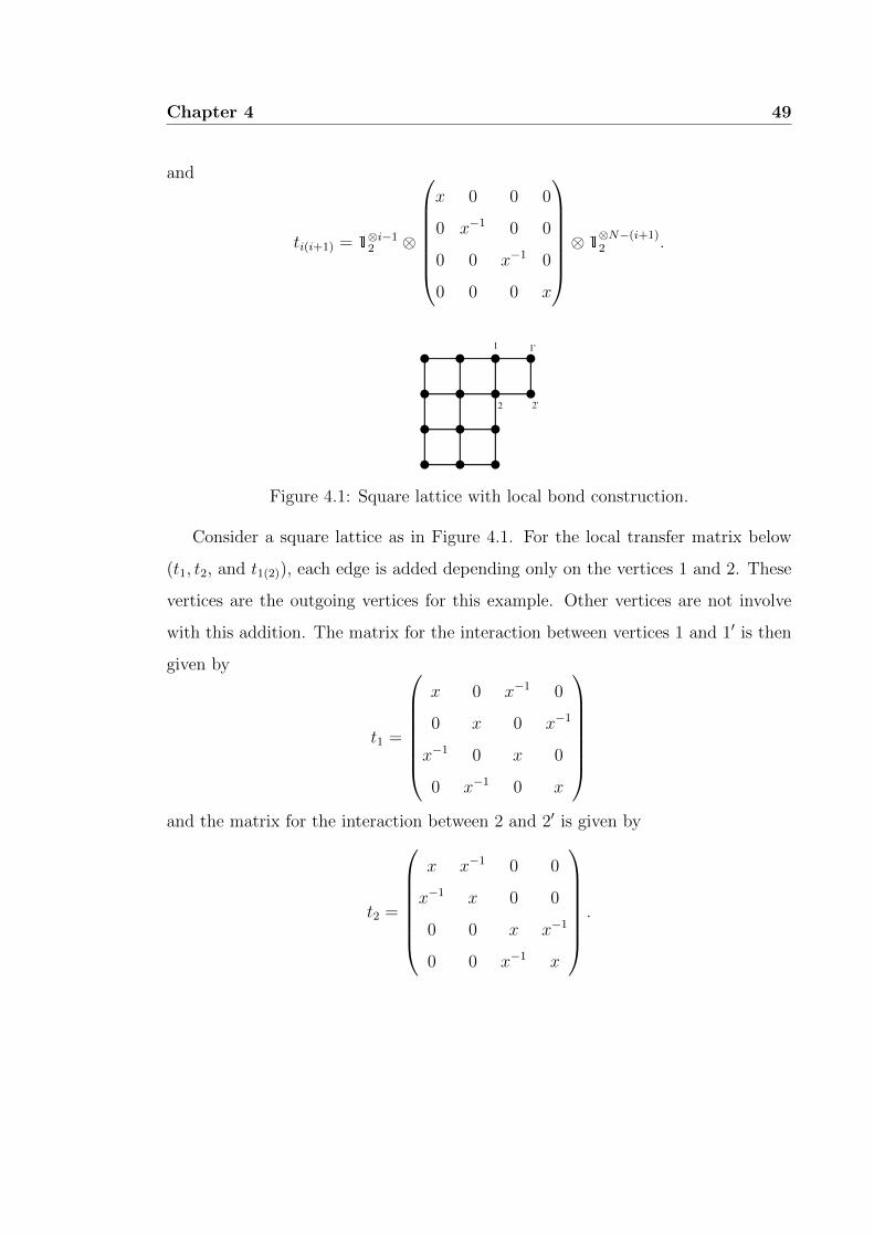
Chapter 4 49

and

ti(i+1) = 1⊗i−12 ⊗

x 0 0 0

0 x−1 0 0

0 0 x−1 0

0 0 0 x

⊗ 1⊗N−(i+1)2 .

1 1'

2 2'

Figure 4.1: Square lattice with local bond construction.

Consider a square lattice as in Figure 4.1. For the local transfer matrix below

(t1, t2, and t1(2)), each edge is added depending only on the vertices 1 and 2. These

vertices are the outgoing vertices for this example. Other vertices are not involve

with this addition. The matrix for the interaction between vertices 1 and 1′ is then

given by

t1 =

x 0 x−1 0

0 x 0 x−1

x−1 0 x 0

0 x−1 0 x

and the matrix for the interaction between 2 and 2′ is given by

t2 =

x x−1 0 0

x−1 x 0 0

0 0 x x−1

0 0 x−1 x

.

50 Chapter 4

The matrix interaction between 1′ and 2′ is then given by

t1(2) =

x 0 0 0

0 x−1 0 0

0 0 x−1 0

0 0 0 x

.

The above matrices are called local transfer matrices.

We can express a transfer matrix in this form,

T = V1 V2

=

(N∏i=1

ti

)(N∏i=1

ti(i+1)

)(4.2)

where tN(N+1) = tN(1) for a periodic boundary condition in vertical direction.

Example 4.1.1. Let N = 5, then the transfer matrix is given by

T = t1t2t3t4t5t1(2)t2(3)t3(4)t4(5)t5(1).

Theorem 4.1.1 (Perron-Frobenius theorem). Let A be a d-dimensional positive

matrix. Then there exist a unique largest magnitude eigenvalue λ which is itself

positive. The associated eigenvector can be chosen to be positive.

See [69] for the proof.

Suppose that a transfer matrix T has dimension d with real value β. The matrix

T is symmetric and positive since it is associated with real and positive Hamiltonian

function. This allow us to diagonalise matrix T by similarity transformation [13,

p. 549]. For any matrix T , there exist a matrix S such that a diagonal matrix

T = ST S−1. This transform

T −→ ST S−1.

By this similarity transformation, for any M ∈ N,

T M = S−1ST S−1ST S−1S · · ·

Chapter 4 51

with

T = ST S−1 =

λ1 0 · · · 0

0 λ2 · · · 0...

.... . .

...

0 0 · · · λd

(4.3)

where λi are the eigenvalues of the matrix T . This gives

T M = S−1

λM1 0 · · · 0

0 λM2 · · · 0...

.... . .

...

0 0 · · · λMd

S . (4.4)

Recall the eigenvalue and eigenvector relation T v = λ v. The ket-vector |i >

has relation T |i >= λi |i > and the bra-vector < j| has relation < j| T =< j|λj,

such that

< i|j >= δij and |i >< j| = 1d

for any i, j = 1, 2, . . . , d and 1d is the d-dimensional identity matrix.

Example 4.1.2. Let T be the transfer matrix and ai, bi ∈ R are associated to any

basis vectors |i > and < j|. For some ai and bi we could have a basis vector given

by equation below. (1 1 · · · 1

)ᵀ=

d−1∑i=0

ai |i >

and (1 1 · · · 1

)=

d−1∑j=0

bj < j| .

By induction,

T |i > = λi |i >,

T 2 |i > = λi T |i >

= λ2i |i > .

52 Chapter 4

Then,

T M−1 |i > = λM−2i T |i >

= λM−2i λi T |i >

= λM−1i |i > .

Hence

T M |i > = λMi |i > .

Then we may have a partition function given by

Z =(

1 1 · · · 1)T M

(1 1 · · · 1

)ᵀ=

d−1∑j=0

bj < j| T Md−1∑i=0

ai |i >

=d−1∑j=0

bj < j|d−1∑i=0

aiλMi |i >

=d−1∑i,j=0

aibjλMi < j|i >

=d−1∑i,j=0

aibjλMi δij

=d−1∑i=0

aibiλMi .

By Perron-Frobenius theorem 4.1.1 there exist a unique largest eigenvalue for

any positive matrix. Denote λ0 as the largest eigenvalue, we have

Z = a0b0λM0 +

d−1∑i=1

aibiλMi (4.5)

= λM0

(a0b0 +

d−1∑i=1

aibi

(λiλ0

)M). (4.6)

Let λi be the eigenvalues of T , equivalently, for N by M lattice, the partition

Chapter 4 53

function

Z = tr(T M) (4.7)

=d−1∑i=0

λMi (4.8)

= λM0

(1 +

d−1∑i=1

(λiλ0

)M). (4.9)

For M →∞, the other eigenvalues give only small contribution which leads to

Z ∼ λM0 .

One approach for this exact solution was studied by Kaufman [40]. Kaufman

describes the relation between a transfer matrix problem with a rotational matrix.

Both matrices are linked by matrix algebra. From this relation, the eigenvalue of

a suitable rotational matrix is equal to the eigenvalue of a transfer matrix. See

formulation of this relationship in detail in [92, p. 70 – 86].

We briefly present parts of the derivation of the eigenvalue λ in Appendix §B.

This derivation gives

λM =N∏k=1

M∏r=1

(K − 2(cos(2πk/N) + cos(2πr/M))

)(4.10)

where

K =(1 + e−4β)2

e−2β(1− e−4β). (4.11)

Then we have,

ZNM ∼ λM

=N∏k=1

M∏r=1


). (4.12)

For y = e2β and C = cos(2πk/N)+cos(2πr/M), each factor in (4.12) can be written

54 Chapter 4

in a polynomial form when Z = 0. We can find the zeros for each factor where

K − 2(cos(2πk/N) + cos(2πr/M) = 0

e−8β + 2Ce−6β + 2e−4β − 2Ce−2β + 1 = 0

y−4 + 2Cy−3 + 2y−2 − 2Cy−1 + 1 = 0

y4 − 2Cy3 + 2y2 + 2Cy + 1 = 0 (4.13)

for any N by M square lattice with k = 1, 2, ..., N and r = 1, 2, ...,M .

4.2 Ising model on finite lattice case

In this section the zeros of the partition function are plotted in the complex-e2β

Argand plane for Ising model on square lattice. The zeros are computed by the

Newton-Raphson method [81]. The Onsager’s square lattice Ising model has a

periodic boundary condition in the vertical and horizontal directions.

The partition function is derived from equation (4.13) (we refer to Appendix

§B). Since the size is finite, the partition function has positive coefficients. Its zeros

will always lie off the real axis. The closest zeros to the real axis (we call endpoints)

move closer to the real axis as the size increases.

Figures 4.2 to 4.5 show the zeros distributions for Ising model on square lattices

with N = M = 14, 90, 99, 100. Figure 4.3b for example is the enlargement for

N = 90 zeros distribution near the ferromagnetic region (explained later in § 4.5).

We can see that the zeros are very close to the real axis. These zeros distributions

form a pattern of two circles as we increase the lattice sizes. Each distribution has

subsets of points with zeros located exactly on two circles. These two circles are the

loci of the zeros for the square lattice Ising model [50, 99].

At thermodynamic limit, the zeros distribution is manifested by the two circles

shown in Figure 4.6. One of the circles cut the real axis at the critical point 1 +√

2.

Chapter 4 55

-2

-1.5

-1

-0.5

0

0.5

1

1.5

2

-2 -1 0 1 2

14x14

(a)

-0.1

0

0.1

0.2

0.3

0.4

0.5

0.6

2 2.1 2.2 2.3 2.4 2.5 2.6

14x14

(b)

Figure 4.2: Zeros plane for 14 by 14 square lattice, a) complete distribution and b)a blow up picture near real axis.

-2

-1.5

-1

-0.5

0

0.5

1

1.5

2

-2 -1 0 1 2

90x90

(a)

-0.1

0

0.1

0.2

0.3

0.4

0.5

0.6

2 2.1 2.2 2.3 2.4 2.5 2.6

90x90

(b)


-2

-1.5

-1

-0.5

0

0.5

1

1.5

2

-2 -1 0 1 2

99x99

(a)

-0.1

0

0.1

0.2

0.3

0.4

0.5

0.6

2 2.1 2.2 2.3 2.4 2.5 2.6

99x99

(b)


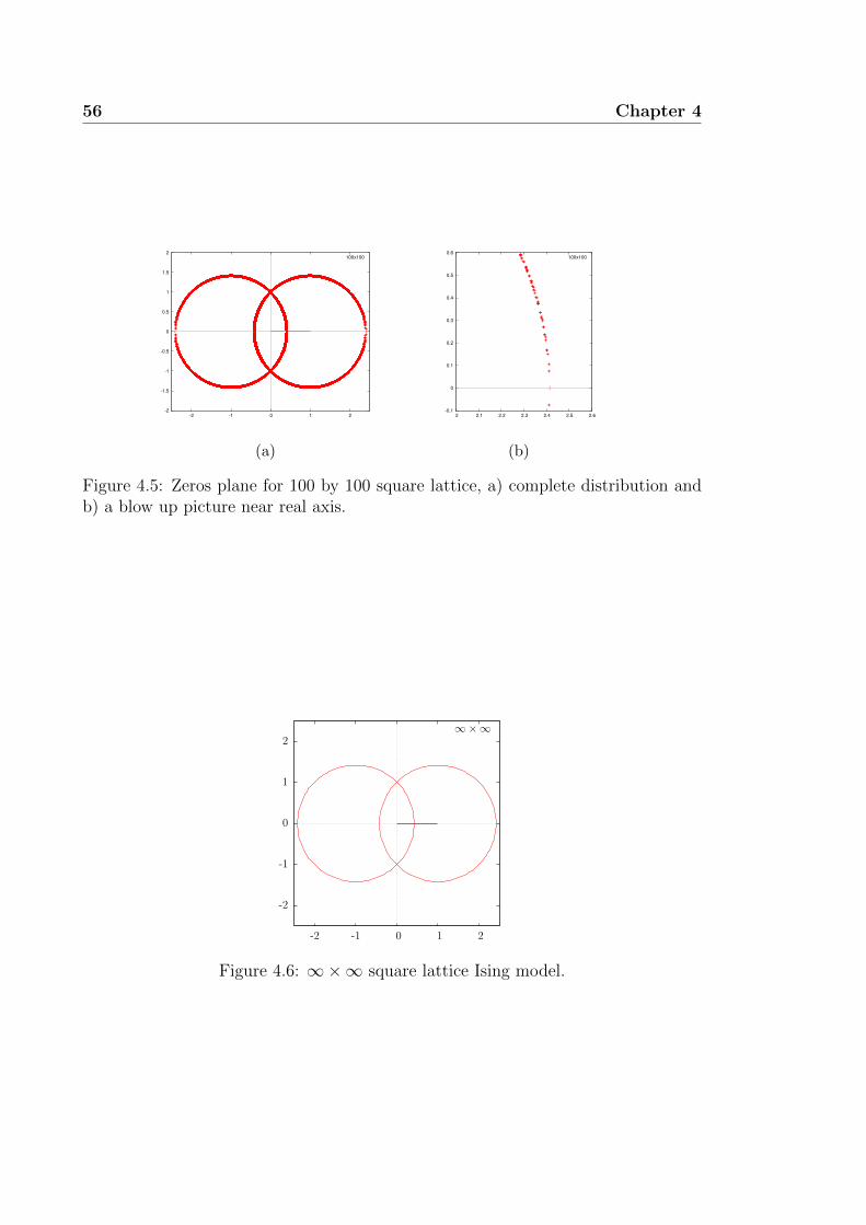
56 Chapter 4

-2

-1.5

-1

-0.5

0

0.5

1

1.5

2

-2 -1 0 1 2

100x100

(a)

-0.1

0

0.1

0.2

0.3

0.4

0.5

0.6

2 2.1 2.2 2.3 2.4 2.5 2.6

100x100

(b)

Figure 4.5: Zeros plane for 100 by 100 square lattice, a) complete distribution andb) a blow up picture near real axis.

-2

-1

0

1

2

-2 -1 0 1 2

∞×∞

Figure 4.6: ∞×∞ square lattice Ising model.

Chapter 4 57

4.3 Finite size effect

The list of zeros distribution of Ising model in previous section (§ 4.2) gives the

evidence that the lattice size has significant effect on the zeros distribution especially

in determining the analytic structure of the zeros distribution. We will see variety of

analytic structure of the finite case with respect to the specific boundary condition

explained later in § 5.1.

Here we consider a simple function for visualising the finite size effect on the

locus of zeros in the complex plane. For example, consider a toy model [58] where

N ∈ N and

Z = xN + 1. (4.14)

The partition function can be written in its zeros form [86] i.e.

Z =N−1∏r=0

(x− e

iπN

(1+2r)).

Example 4.3.1. Suppose N = 4, then

Z = xN + 1

= x4 + 1.

The zeros of Z is given by

x4 + 1 = 0

x = 4√−1

∼ eiπ4

(1+2r); r = 0, 1, 2, 3.

Similarly, suppose N = 10, then

x10 + 1 = 0

x = 10√−1

∼ eiπ10

(1+2r); r = 0, 1, 2, ..., 9.

58 Chapter 4

-1.5

-1

-0.5

0

0.5

1

1.5

-1.5 -1 -0.5 0 0.5 1 1.5

N=10

(a)

-1.5

-1

-0.5

0

0.5

1

1.5

-1.5 -1 -0.5 0 0.5 1 1.5

N=20

(b)

-1.5

-1

-0.5

0

0.5

1

1.5

-1.5 -1 -0.5 0 0.5 1 1.5

N=50

(c)

-1.5

-1

-0.5

0

0.5

1

1.5

-1.5 -1 -0.5 0 0.5 1 1.5

N=70

(d)

Figure 4.7: Zeros plane for N = 10, 20, 50 and 70.

Figure 4.7 shows the zeros distributions for different value of N from equation

(4.14). The zeros are equally distributed in this plane and the gap between two

zeros is decreases as N increases. This distribution has locus of a unit circle where

the zeros cut the real axis at Re(x) = ±1.

The zeros distribution for the Ising model shows similar behaviour as suggested

by the example in Figure 4.7. The zeros for different value of N are distributed in

a specific pattern and become denser as N increases. The endpoints of the zeros

move closer to the real axis.

We show in Figures 4.8 and 4.9 the distributions for the Ising model on square and

cubic lattices in some value of N . Both figures are called the overlay distributions

where we plot the result from two different cases in one complex plane. Note well

here, though, that these results follow a very careful and special choice of boundary

conditions without which the locus of zeros will also experience finite size effect.

Chapter 4 59

-2

-1

0

1

2

-2 -1 0 1 2

14x14

8x8

(a)

0

0.5

1

1.5

2

2.5

0 0.5 1 1.5 2 2.5

14x14

8x8

(b)

Figure 4.8: Overlay distributions on square lattices with different system size N .

-2

-1.5

-1

-0.5

0

0.5

1

1.5

2

-2 -1.5 -1 -0.5 0 0.5 1 1.5 2

5x4x10’

3x4x10’

Figure 4.9: Overlay distributions on cubic lattices with different system size N .

60 Chapter 4

4.4 Duality relation

We discuss a duality relation for the Ising model in this section. Recall y = e2β

and the duality transformation [58] of the Ising model described in § 2.2 is given by

relation1

y→ y − 1

y + 1.

We can study this relation and see the change in the locus of the zeros. For

a, b ∈ R, y = a+ bi, let1

y=y − 1

y + 1(4.15)

where y is a complex number and y is its complex conjugate. Then

1

a+ bi=

a− bi− 1

a− bi+ 1

a− bi+ 1 = (a− bi− 1)(a+ bi)

a2 − 2a+ b2 − 1 = 0

b = ±√

2a− a2 + 1. (4.16)

Recall that the exact solution has locus of two circles where one of the

interception points is at 1 +√

2. Plotting relation (4.16) will give a structure which

is the same with one of the circles in the exact solution. At real axis when b = 0,

we have a = 1 +√

2 that is equal to the point in the exact solution.

From the above observation, the circle in the exact solution that has interception

point at 1 +√

2 is invariant under a duality transformation. The zeros which are

fixed under the duality transformation (4.15) are just a complex conjugates of one

another. The duality circle has radius√

2 centered at (1,0) in the complex plane.

An overlay plot of (4.16) with the zeros from specific case of square lattice will

highlight the invariance property. The majority of zeros lie in part of the plane,

exactly on an arc of a circle but not all of the zeros are confined to the circle. Figure

4.10 plot the dual case of a 14 by 14 Ising square lattice together with the complex

conjugation circle (4.16). The zeros are computed directly from relation (4.15).

Chapter 4 61

-2

-1

0

1

2

-2 -1 0 1 2

(14x14)

Figure 4.10: Distribution of dual zeros for 14 by 14 Ising square lattice and the circle(4.16).

4.5 Ferromagnetic and antiferromagnetic regions

Here we explain the relation between the complex plane of the zeros distribution

and the ferromagnetic and antiferromagnetic states [41, 46, 68] in a physical system.

The ferromagnetic (ferro) state corresponds to the state where all the molecular

dipoles point in the same direction. Conversely an antiferromagnetic (antiferro)

state corresponds to the state where each molecular dipole tends to point in the

different direction from its neighbours.

Note that the interaction energy J is assumed to be the same for every dipole-

dipole nearest neighbour interaction and x = eβJ . If J > 0, the Hamiltonian function

will be in its lowest energy where all spin variables spin in the same direction. The

system is said to be in the ferromagnetic state. Otherwise, if J < 0, the negative

coupling constant J will force the variables to be anti-align to its neighbour. This

is the antiferromagnetic state.

Since temperature T > 0 gives β > 0, when J > 0, the (0, 1)-region is not

physical i.e. eβJH = 1 for β = 0. Hence the (1,∞)-region corresponds to the

physical state of ferromagnetism. But if J < 0, the e−JβH > 0. Hence the (0, 1)-

region can be interpreted as the antiferro region.

62 Chapter 4

From this chapter, we see that the study of zeros of the partition function allow

us to study the limiting behaviour of the zeros in the complex plane. The zeros

distribution may suggest the limiting behaviour of a bulk system at large enough

lattice size.

For comparison, we describe the result for the 2-state Potts model in different

boundary conditions. We present their zeros distributions and observe any zeros

structure in the next chapter.

Chapter 5

The Q-state Potts model partition

function zeros

This chapter presents the zeros for the Q-state Potts model partition function for

several lattice types and Q = 2, 3, 4, 5, 6. Recall that the partition function for a

given lattice Λ = (V,E, f) and Q is defined as

ZPotts =∑

σ∈Hom(V,Q)

exp(−βHPotts(σ))

whereHPotts is as in Definition 1.1.5. We consider two- and three-dimensional lattice

graphs as described in Chapter 2.

The zeros are plotted in a complex-eβ Argand plane for observation. The zeros

distributions for a given lattice type are arranged in increasing sizes.

As discussed in § 2.1.1 and § 4.2, we may search for the convergence sequence

of analytic structure from the zeros distribution. We search for the structure or

pattern formed by the collection of zeros in the complex plane.

The partition function calculation for lattices bigger than the previously studied

case [9, 23, 58, 60, 77] will be one new finding in this thesis. In § 2.1.1 we explained

why results for larger finite lattice sizes of a given type are valuable.

Recall in Chapter 4, we showed the emergence of pattern of zeros structure

63

64 Chapter 5

as we change the lattice size. Then we relate them to the critical point in the

thermodynamic limit in the example of square lattice Ising model [40].

x

y

Figure 5.1: Number of row vertices denoted y (also we denote this y = N) andcolumn vertices denoted x (also we denote this x = M).

Main results

Table 5.1: Largest sizes for all considered lattice types including the new results(highlighted in grey).

Q 2 3 4 5 6

Square20x20’ 13x13’ 10x10’ 8x9’ 8x9’

14x14’ 11x13’ 9x9’ 9x9’15x17’ 12x13’ 10x13’

Triangular

13x13’ 13x13’ 7x7’ 7x7’14x14’ 14x17’ 8x8’ 8x8’15x15’ 9x9’

10x10’11x13’

Hexagonal 18x18’ 12x12’ 10x13’Cubic 5x5x5’ 3x4x10’ 3x3x10’ 3x3x5’ 3x3x6’

Tetragonal (hcp)3x3x7’ 3x3x7’3x4x7’ 3x4x7’4x4x7’

Octagonal (fcc)3x3x7’ 3x3x7’3x4x7’ 3x4x7’4x4x7’

First we give the notation for specifying a graph Λ in the case of square or

cubic lattice type. Let Nx, Ny, Nz correspond to the number of vertices in the three

Chapter 5 65

directions x, y and z. We write Nx × Ny × Nz for periodic boundary conditions in

each direction. A notation with prime such as N ′z for z direction represents the open

boundary condition. Note that Ny ×Nx and Nx ×Ny ×Nz represent the two- and

three-dimensional case respectively. We write (Ny × Nx) for the dual lattice and

(Ny ×Nx)′ corresponds to the self-dual lattice as defined in § 2.2.

Table 5.1 summarises the lattices considered in this thesis for Q-state Potts

models. Each result of zeros distribution for different lattice graph is discussed in

separate section.

Three new results extending the existing literature such as in [59, 92] for the

3-state Potts model on square lattice are produced for N = 13, 14, 15. We have also

produced new results for the triangular lattice for 2-, 3-, 4- and 5-state Potts model.

The octagonal and tetragonal lattices are another new cases we have considered for

this thesis.

We have considered all computable cases up to specific lattice sizes (based on our

current computing resources). For cubic lattice however, we could not produce a new

result due to computing limitation. The number of configurations in one layer of the

5× 6× 5′ for example, contains 30 vertices (5 column in z-axis and 6 row in y-axis).

This equivalent to 230 configuration states. This huge number of states however,

exceed the maximum value of the standard integer in the computer. For comparison,

each 1 step expansion in the square lattice involves only an increment of Q2N . This

number of configurations is much smaller than the lattice layer configuration state

for cubic lattice i.e. for Q2N2

.

Each case except for the 2-state Potts model has periodic vertical and open

horizontal boundary conditions. We consider this type of boundary condition since

we could produce a zeros distribution that is not fuzzy especially in the ferromagnetic

region. This boundary condition also has translation symmetry in the vertical

direction which is essential to reduce the number of computations. The computer

program for computing the partition function in this thesis is designed to use a

matrix-vector multiplication. This strategy is implemented to reduced the memory

66 Chapter 5

usage in the computing resources.

Previous results

The Onsager’s partition function for square lattice Ising model allows us to find the

zeros distribution for any square lattice size (but in general for boundary conditions

different from ours − as given in Chapter 4). The paper by Chen, Hu and Wu [16] is

another example for the study on square lattice with self-dual boundary conditions.

The previous largest result for the 3-state Potts model on square lattice was due

to Martin [59] where he produced 12 × 13′ square lattice. Similar to this, Valani

also considered the 3-state Potts model on a (12 × 16)′ self-dual square lattice. In

addition to this, Matveev and Shrock [61] in the earlier paper showed the result for

10 by 8 lattice for several boundary conditions. Valani in his thesis [92] produced

the zeros distributions for state Q = 2, 3, 4, 5, 6 for different boundary conditions.

Furthermore, the Ising model on hexagonal lattice had been previously studied

by Feldman, Shrock and Tsai [25] on 24 by 18 and also 20 by 20 lattice sizes.

They also considered for the Q = 3, 4 on hexagonal lattice particularly for 12× 16′

lattice. By duality transformation, Feldman, Guttmann, Jensen, Shrock and Tsai

[24] plotted the zeros distribution for triangular lattice up to boundary condition

similar to 12 × 9′ and 10 × 10′ for Q = 2 and 6 × 8′ for Q = 3, 4. They consider

several types of boundary condition including all periodic and also mixed periodic

and open boundary conditions. Martin and Maillard [60] on the other hand extended

the triangular lattice for 3-state Potts model for 108 sites i.e. 12 by 9 lattice.

In addition, Pearson [77] described the Ising model on 4×4×4 cubic lattice and

then Bhanot and Sastry [9] presented two steps larger with 4× 5× 5′ cubic lattice.

The latest and largest lattice for the cubic case however still due to Valani [92]. In

his thesis, he discussed a sequence of cubic lattices up to 5× 5× 10′.

Chapter 5 67

5.1 2-state Potts (Ising) model on square lattice

− revisited

As a check for the programs we start with running them on the exactly solved case

of square lattice 2-state (Ising) Potts model. The comparison between the result of

zeros distribution at limit and at finite sizes is also presented here. We consider the

finite case restricted to some boundary conditions.

-2

-1

0

1

2

-2 -1 0 1 2

14x14

(a)

-2

-1

0

1

2

-2 -1 0 1 2

50x50

(b)

Figure 5.2: Square lattice Ising model with Onsager’s partition function a) 14× 14and b) 50× 50.

-2

-1

0

1

2

-2 -1 0 1 2

∞×∞

Figure 5.3: ∞×∞ square lattice Ising model.

The square lattice Ising model zeros distribution is discussed in § 4.2 where the

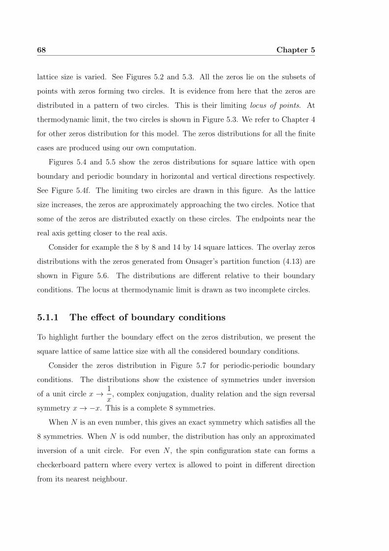
68 Chapter 5

lattice size is varied. See Figures 5.2 and 5.3. All the zeros lie on the subsets of

points with zeros forming two circles. It is evidence from here that the zeros are

distributed in a pattern of two circles. This is their limiting locus of points. At

thermodynamic limit, the two circles is shown in Figure 5.3. We refer to Chapter 4

for other zeros distribution for this model. The zeros distributions for all the finite

cases are produced using our own computation.

Figures 5.4 and 5.5 show the zeros distributions for square lattice with open

boundary and periodic boundary in horizontal and vertical directions respectively.

See Figure 5.4f. The limiting two circles are drawn in this figure. As the lattice

size increases, the zeros are approximately approaching the two circles. Notice that

some of the zeros are distributed exactly on these circles. The endpoints near the

real axis getting closer to the real axis.

Consider for example the 8 by 8 and 14 by 14 square lattices. The overlay zeros

distributions with the zeros generated from Onsager’s partition function (4.13) are

shown in Figure 5.6. The distributions are different relative to their boundary

conditions. The locus at thermodynamic limit is drawn as two incomplete circles.

5.1.1 The effect of boundary conditions

To highlight further the boundary effect on the zeros distribution, we present the

square lattice of same lattice size with all the considered boundary conditions.

Consider the zeros distribution in Figure 5.7 for periodic-periodic boundary

conditions. The distributions show the existence of symmetries under inversion

of a unit circle x → 1

x, complex conjugation, duality relation and the sign reversal

symmetry x→ −x. This is a complete 8 symmetries.

When N is an even number, this gives an exact symmetry which satisfies all the

8 symmetries. When N is odd number, the distribution has only an approximated

inversion of a unit circle. For even N , the spin configuration state can forms a

checkerboard pattern where every vertex is allowed to point in different direction

from its nearest neighbour.

Chapter 5 69

-2

-1

0

1

2

-2 -1 0 1 2

8x8’

(a)

-2

-1

0

1

2

-2 -1 0 1 2

9x9’

(b)

-2

-1

0

1

2

-2 -1 0 1 2

11x11’

(c)

-2

-1

0

1

2

-2 -1 0 1 2

12x12’

(d)

-2

-1

0

1

2

-2 -1 0 1 2

13x13’

(e)

-2

-1

0

1

2

-2 -1 0 1 2

14x14’

(f)

Figure 5.4: 2-state, square lattice with periodic-open boundary conditions.

70 Chapter 5

-2

-1

0

1

2

-2 -1 0 1 2

15x15’

(a)

-2

-1

0

1

2

-2 -1 0 1 2

16x16’

(b)

-2

-1

0

1

2

-2 -1 0 1 2

17x17’

(c)

-2

-1

0

1

2

-2 -1 0 1 2

18x18’

(d)

-2

-1

0

1

2

-2 -1 0 1 2

19x19’

(e)

-2

-1

0

1

2

-2 -1 0 1 2

20x20’

(f)

Figure 5.5: 2-state, square lattice with periodic-open boundary conditions (cont.).

Chapter 5 71

-2

-1

0

1

2

-2 -1 0 1 2

8x8’

ons-8x8

-2

-1

0

1

2

-2 -1 0 1 2

14x14’

ons-14x14

Figure 5.6: Zeros distributions for N = 8, 14 square lattices: ons-8×8 and ons-14×14are generated from the Onsager’s partition function (4.13).

-2

-1

0

1

2

-2 -1 0 1 2

5x5

(a)

-2

-1

0

1

2

-2 -1 0 1 2

6x6

(b)

-2

-1

0

1

2

-2 -1 0 1 2

7x7

(c)

-2

-1

0

1

2

-2 -1 0 1 2

8x8

(d)

Figure 5.7: 2-state, square lattice with periodic-periodic boundary conditions.

72 Chapter 5

-2

-1

0

1

2

-2 -1 0 1 2

(4x4)’

(a)

-2

-1

0

1

2

-2 -1 0 1 2

(5x5)’

(b)

-2

-1

0

1

2

-2 -1 0 1 2

(6x6)’

(c)

-2

-1

0

1

2

-2 -1 0 1 2

(7x7)’

(d)

-2

-1

0

1

2

-2 -1 0 1 2

(8x8)’

(e)

-2

-1

0

1

2

-2 -1 0 1 2

(9x9)’

(f)

Figure 5.8: 2-state, square lattice with self-dual boundary conditions.

Chapter 5 73

Figure 5.8 shows the distribution for the 2-state Potts model on square lattice

with self-duality condition. A smooth zeros distribution is forming a pattern of a

circle in the physical region.

-2

-1

0

1

2

-2 -1 0 1 2

6x6

(a)

-2

-1

0

1

2

-2 -1 0 1 2

6x6’

(b)

-2

-1

0

1

2

-2 -1 0 1 2

(6x6)’

(c)

Figure 5.9: 2-state, square lattice with different boundary conditions.

Figure 5.9 shows the zeros distributions for the 6 by 6 square lattice with different

boundary conditions. The zeros for model with mixed periodic and open boundary

conditions (Figure 5.9b) are distributed around two circles but mostly are not exactly

lie on the limiting two circles. In contrast, the zeros for self-dual lattice case (Figure

5.9c) shows a clear line distribution especially in the positive real axis part (first

and forth quadrant). The two circles are apparent even at small lattice size.

74 Chapter 5

5.2 3-state Potts model on square lattice

Here we present the zeros distribution for the 3-state Potts model on a square

lattice with periodic vertical and open horizontal boundary conditions. The study

for higher state Q > 2 is interesting because until now there is no exact solution

found for these cases.

In Figure 5.10, a structure which we call a branch can be seen in the non-physical

axis (−∞, 0]. This branch is related to the (0, 1) antiferro region by the duality

transformation (2.11). The increment in size shows multiple branch structures start

to get closer to the real axis. Close to real axis, we observe an arm of dense zeros

in the antiferro region. In the first and forth quadrants, an arc of a smooth circle is

also observed. Note that the different structure between odd and even N is due to

the finite size effect.

See particularly the new results for N = 13, 14 and 15 in Figures 5.12 to 5.14.

Figure 5.15a shows the overlay distribution of zeros for N = 12, 13 and Figure 5.15b

for N = 14, 15. The different in the non-physical region is particularly obvious

between these figures (also see Figure 5.16).

Nevertheless, the zeros curves are the same for all cases at the (1,∞) ferro

region except that their ending points have different value. The endpoint here is

represented by the closest point near the real axis. The biggest size N = 15 has the

closest point to this axis as compared to other sizes N < 15.

Figures 5.17 and 5.18 in addition emphasize the enlargement of the zeros

distribution for N = 12, 13, 14 and 15 especially for the physical regions.

Correspondingly, the zeros structure in the antiferro region moves closer to the

real axis.

Although we expect that the closest point to the real axis comes from the largest

case, Figure 5.16 shows otherwise. The closest point in this region is represented by

the zeros from N = 14. As discussed earlier, we know that the partition function is

always affected by the finite size effect.

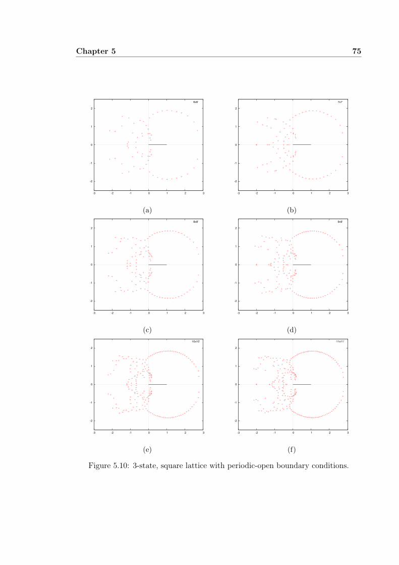
Chapter 5 75

-2

-1

0

1

2

-3 -2 -1 0 1 2 3

6x6’

(a)

-2

-1

0

1

2

-3 -2 -1 0 1 2 3

7x7’

(b)

-2

-1

0

1

2

-3 -2 -1 0 1 2 3

8x8’

(c)

-2

-1

0

1

2

-3 -2 -1 0 1 2 3

9x9’

(d)

-2

-1

0

1

2

-3 -2 -1 0 1 2 3

10x10’

(e)

-2

-1

0

1

2

-3 -2 -1 0 1 2 3

11x11’

(f)


76 Chapter 5

-2

-1

0

1

2

-3 -2 -1 0 1 2 3

12x12’


-2

-1

0

1

2

-3 -2 -1 0 1 2 3

13x13’


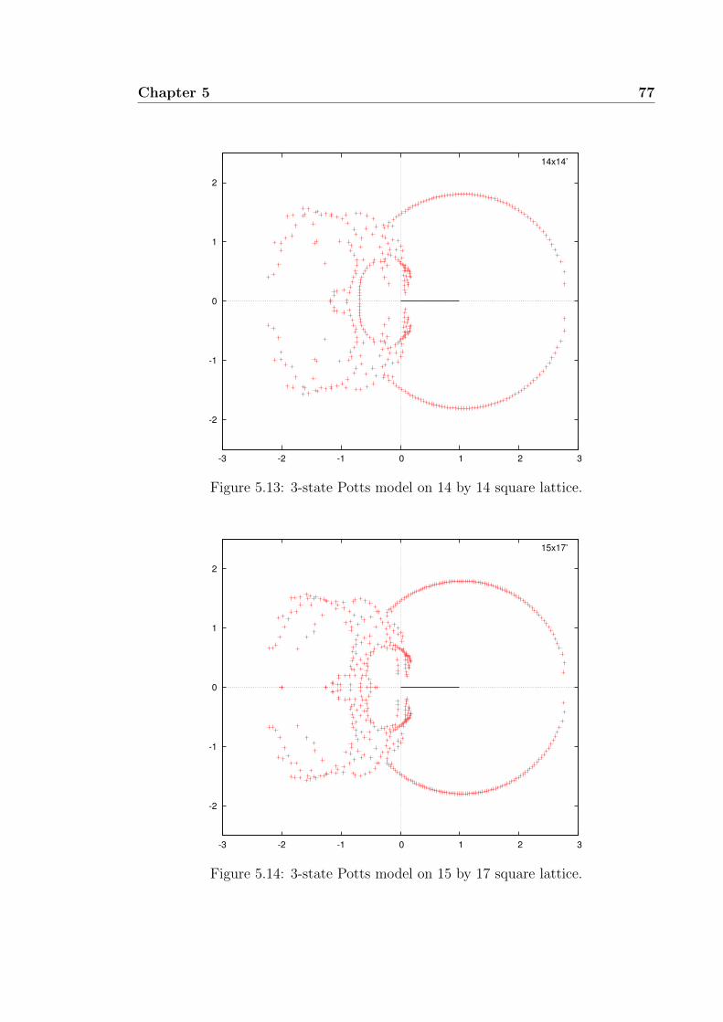
Chapter 5 77

-2

-1

0

1

2

-3 -2 -1 0 1 2 3

14x14’


-2

-1

0

1

2

-3 -2 -1 0 1 2 3

15x17’


78 Chapter 5

-2

-1

0

1

2

-3 -2 -1 0 1 2 3

12x12’

13x13’

(a)

-2

-1

0

1

2

-3 -2 -1 0 1 2 3

14x14’

15x17’

(b)

Figure 5.15: 3-state Potts model on a) 12 × 12′ and 13 × 13′ and b) 14 × 14′ and15× 17′ square lattices.

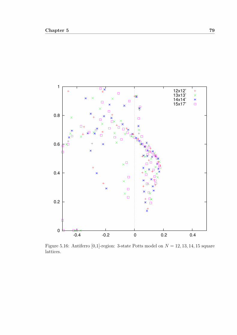
Chapter 5 79

0

0.2

0.4

0.6

0.8

1

-0.4 -0.2 0 0.2 0.4

12x12’

13x13’

14x14’

15x17’

Figure 5.16: Antiferro [0,1]-region: 3-state Potts model on N = 12, 13, 14, 15 squarelattices.

80 Chapter 5

-2

-1

0

1

2

-1 -0.5 0 0.5 1 1.5 2 2.5 3

12x12’

13x13’

Figure 5.17: Zoom in: 3-state Potts model on 12× 12′ and 13× 13′ square lattices.

Chapter 5 81

-2

-1

0

1

2

-1 -0.5 0 0.5 1 1.5 2 2.5 3

14x14’

15x17’

Figure 5.18: Zoom in: 3-state Potts model on 14× 14′ and 15× 17′ square lattices.

82 Chapter 5

5.2.1 Self-duality partition function

We investigate the duality transformation for the 3-state Potts model on square

lattice in this section.

On an infinite lattice, the square lattice is self-dual where the partition function

is invariant under the duality transformation (2.11) given by

x↔ x+ (Q− 1)

x− 1. (5.1)

Similarly, this duality transformation gives the same mapping for the zeros of the

partition function. But for a finite lattice the effect of the transformation depends

on the boundary conditions. However the boundary effect will be reduced at large

lattice size when the partition function is approximately self-dual.

The zeros of the Ising model partition function lie on the locus of two circles

where the dual for each zero must be its complex conjugate. Recall from § 4.4 that

in this model the duality circle has radius√

2 centered at (1,0) in the complex plane.

Similarly, for the 3-state Potts model we may deduce its locus of zeros by this duality

transformation. In this case the circle has radius√

3 centered at (1,0) (see Figures

5.19 and 5.20).

Generally, a self-dual polynomial partition function may be constructed from a

linear combination of partition functions from various boundary conditions [26, 54,

55]. Recall also the dual graph relation in § 2.2. Let Zd be the dual of Z given by

Z

(x+ (Q− 1)

x− 1

)= Zd(x).

Here we will construct the linear combination of partition functions, denoted Z∗

which preserve the self-duality condition. Let M ∈ N be the degree of Z, then

Z∗(x) =1

(x− 1)M/2Z(x) + Zd(x) (5.2)

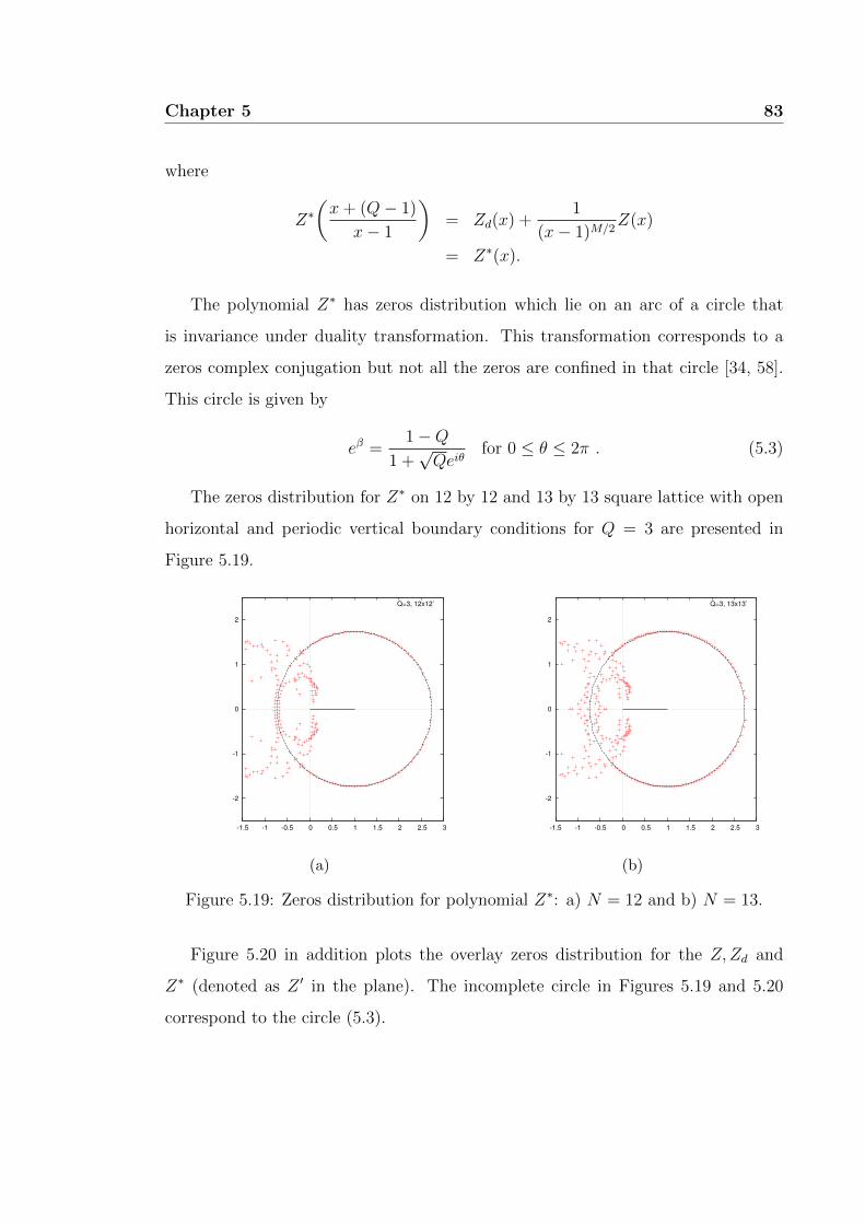
Chapter 5 83

where

Z∗(x+ (Q− 1)

x− 1

)= Zd(x) +

1

(x− 1)M/2Z(x)

= Z∗(x).

The polynomial Z∗ has zeros distribution which lie on an arc of a circle that

is invariance under duality transformation. This transformation corresponds to a

zeros complex conjugation but not all the zeros are confined in that circle [34, 58].

This circle is given by

eβ =1−Q

1 +√Qeiθ

for 0 ≤ θ ≤ 2π . (5.3)

The zeros distribution for Z∗ on 12 by 12 and 13 by 13 square lattice with open

horizontal and periodic vertical boundary conditions for Q = 3 are presented in

Figure 5.19.

-2

-1

0

1

2

-1.5 -1 -0.5 0 0.5 1 1.5 2 2.5 3

Q=3, 12x12’

(a)

-2

-1

0

1

2

-1.5 -1 -0.5 0 0.5 1 1.5 2 2.5 3

Q=3, 13x13’

(b)

Figure 5.19: Zeros distribution for polynomial Z∗: a) N = 12 and b) N = 13.

Figure 5.20 in addition plots the overlay zeros distribution for the Z,Zd and

Z∗ (denoted as Z ′ in the plane). The incomplete circle in Figures 5.19 and 5.20

correspond to the circle (5.3).

84 Chapter 5

-2

-1

0

1

2

3

-2 -1 0 1 2 3

Zd

Z

Z’

(a)

-2

-1

0

1

2

3

-2 -1 0 1 2 3

Zd

Z

Z’

(b)

Figure 5.20: Zeros distribution for polynomial Z,Zd and Z∗ = Z ′: a) N = 14 andb) N = 15.

Chapter 5 85

5.3 Q ≥ 4, square lattice Potts model

Here we consider the square lattice Potts model with state Q = 4, 5 and 6.

-3

-2

-1

0

1

2

3

-3 -2 -1 0 1 2 3

7x7’

(a)

-3

-2

-1

0

1

2

3

-3 -2 -1 0 1 2 3

8x8’

(b)

-3

-2

-1

0

1

2

3

-3 -2 -1 0 1 2 3

9x9’

(c)

-3

-2

-1

0

1

2

3

-3 -2 -1 0 1 2 3

10x10’

(d)

-3

-2

-1

0

1

2

3

-3 -2 -1 0 1 2 3

11x13’

(e)

-3

-2

-1

0

1

2

3

-3 -2 -1 0 1 2 3

12x13’

(f)


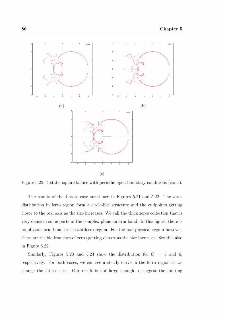
86 Chapter 5

-3

-2

-1

0

1

2

3

-3 -2 -1 0 1 2 3

6x32’

(a)

-3

-2

-1

0

1

2

3

-3 -2 -1 0 1 2 3

7x32’

(b)

-3

-2

-1

0

1

2

3

-3 -2 -1 0 1 2 3

8x32’

(c)

Figure 5.22: 4-state, square lattice with periodic-open boundary conditions (cont.).

The results of the 4-state case are shown in Figures 5.21 and 5.22. The zeros

distribution in ferro region form a circle-like structure and the endpoints getting

closer to the real axis as the size increases. We call the thick zeros collection that is

very dense in some parts in the complex plane an arm band. In this figure, there is

no obvious arm band in the antiferro region. For the non-physical region however,

there are visible branches of zeros getting denser as the size increases. See this also

in Figure 5.22.

Similarly, Figures 5.23 and 5.24 show the distribution for Q = 5 and 6,

respectively. For both cases, we can see a steady curve in the ferro region as we

change the lattice size. Our result is not large enough to suggest the limiting

Chapter 5 87

-3

-2

-1

0

1

2

3

-3 -2 -1 0 1 2 3 4

5x5’

(a)

-3

-2

-1

0

1

2

3

-3 -2 -1 0 1 2 3 4

6x6’

(b)

-3

-2

-1

0

1

2

3

-3 -2 -1 0 1 2 3 4

7x7’

(c)

-3

-2

-1

0

1

2

3

-3 -2 -1 0 1 2 3 4

8x9’

(d)

-3

-2

-1

0

1

2

3

-3 -2 -1 0 1 2 3 4

9x9’

(e)

-3

-2

-1

0

1

2

3

-3 -2 -1 0 1 2 3 4

10x13’

(f)


88 Chapter 5

behaviour especially in the antiferro region, although a circle-like structure is obvious

in the ferro region.

-3

-2

-1

0

1

2

3

-3 -2 -1 0 1 2 3 4

4x4’

(a)

-3

-2

-1

0

1

2

3

-3 -2 -1 0 1 2 3 4

5x5’

(b)

-3

-2

-1

0

1

2

3

-3 -2 -1 0 1 2 3 4

6x6’

(c)

-3

-2

-1

0

1

2

3

-3 -2 -1 0 1 2 3 4

7x7’

(d)

-3

-2

-1

0

1

2

3

-3 -2 -1 0 1 2 3 4

8x9’

(e)

-3

-2

-1

0

1

2

3

-3 -2 -1 0 1 2 3 4

9x9’

(f)


Chapter 5 89

5.4 On triangular and hexagonal lattice

We know from Chapter 2 that the triangular and hexagonal lattice, up to boundary

condition are dual to each other. This means we can get the hexagonal lattice

distribution from the triangular case and vice versa.

Here we consider Q-state Potts models on triangular and hexagonal lattices

with periodic and open boundary conditions in vertical and horizontal directions

respectively.

For the 2-state Potts model on triangular lattice, the zeros distributions shown

in Figures 5.25 and 5.26 have values near a pattern of a double ‘horseshoe’. The

scattered points are due to the boundary condition and the finite size effect. At the

thermodynamic limit, the zeros distribution is expected to be smooth in this locus.

Figure 5.27 shows the zeros distribution for the 3-state Potts model on triangular

lattice. The positive real axis shows the existence of arcs of zeros approaching the

ferro and antiferro regions.

In addition, the zeros distributions of the 4- and 5-state Potts models on

triangular lattice are presented respectively in Figures 5.28 and 5.29. We can see

the line of zeros approaching the real axis in the ferro region as the size increases.

In the 4-state case, we can see some zeros move closer to the antiferro region as

the size increases. This region either has a transition at the origin or interestingly

at small positive value close to origin. A bigger lattice is needed for studying this

region.

The case for 5-state however has a line of zeros approaching the real axis in ferro

region but not in the antiferro region. Here some branches in the non-physical region

move closer to the origin as the size increases.

90 Chapter 5

-2

-1.5

-1

-0.5

0

0.5

1

1.5

2

-2 -1.5 -1 -0.5 0 0.5 1 1.5 2

6x6’

(a)

-2

-1.5

-1

-0.5

0

0.5

1

1.5

2

-2 -1.5 -1 -0.5 0 0.5 1 1.5 2

7x7’

(b)

-2

-1.5

-1

-0.5

0

0.5

1

1.5

2

-2 -1.5 -1 -0.5 0 0.5 1 1.5 2

8x8’

(c)

-2

-1.5

-1

-0.5

0

0.5

1

1.5

2

-2 -1.5 -1 -0.5 0 0.5 1 1.5 2

9x9’

(d)

-2

-1.5

-1

-0.5

0

0.5

1

1.5

2

-2 -1.5 -1 -0.5 0 0.5 1 1.5 2

10x10’

(e)

-2

-1.5

-1

-0.5

0

0.5

1

1.5

2

-2 -1.5 -1 -0.5 0 0.5 1 1.5 2

11x11’

(f)

Figure 5.25: 2-state, triangular lattice with periodic-open boundary conditions.

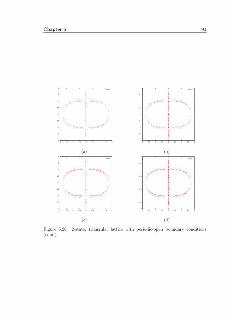
Chapter 5 91

-2

-1.5

-1

-0.5

0

0.5

1

1.5

2

-2 -1.5 -1 -0.5 0 0.5 1 1.5 2

12x12’

(a)

-2

-1.5

-1

-0.5

0

0.5

1

1.5

2

-2 -1.5 -1 -0.5 0 0.5 1 1.5 2

13x13’

(b)

-2

-1.5

-1

-0.5

0

0.5

1

1.5

2

-2 -1.5 -1 -0.5 0 0.5 1 1.5 2

14x14’

(c)

-2

-1.5

-1

-0.5

0

0.5

1

1.5

2

-2 -1.5 -1 -0.5 0 0.5 1 1.5 2

15x15’

(d)

Figure 5.26: 2-state, triangular lattice with periodic-open boundary conditions(cont.).

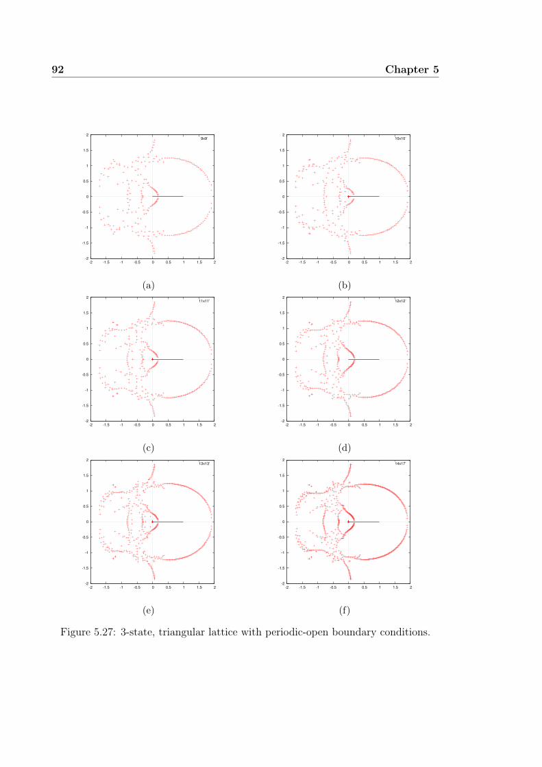
92 Chapter 5

-2

-1.5

-1

-0.5

0

0.5

1

1.5

2

-2 -1.5 -1 -0.5 0 0.5 1 1.5 2

9x9’

(a)

-2

-1.5

-1

-0.5

0

0.5

1

1.5

2

-2 -1.5 -1 -0.5 0 0.5 1 1.5 2

10x10’

(b)

-2

-1.5

-1

-0.5

0

0.5

1

1.5

2

-2 -1.5 -1 -0.5 0 0.5 1 1.5 2

11x11’

(c)

-2

-1.5

-1

-0.5

0

0.5

1

1.5

2

-2 -1.5 -1 -0.5 0 0.5 1 1.5 2

12x12’

(d)

-2

-1.5

-1

-0.5

0

0.5

1

1.5

2

-2 -1.5 -1 -0.5 0 0.5 1 1.5 2

13x13’

(e)

-2

-1.5

-1

-0.5

0

0.5

1

1.5

2

-2 -1.5 -1 -0.5 0 0.5 1 1.5 2

14x17’

(f)


Chapter 5 93

-2

-1.5

-1

-0.5

0

0.5

1

1.5

2

-2 -1.5 -1 -0.5 0 0.5 1 1.5 2 2.5

6x6’

(a)

-2

-1.5

-1

-0.5

0

0.5

1

1.5

2

-2 -1.5 -1 -0.5 0 0.5 1 1.5 2 2.5

7x7’

(b)

-2

-1.5

-1

-0.5

0

0.5

1

1.5

2

-2 -1.5 -1 -0.5 0 0.5 1 1.5 2 2.5

8x8’

(c)

-2

-1.5

-1

-0.5

0

0.5

1

1.5

2

-2 -1.5 -1 -0.5 0 0.5 1 1.5 2 2.5

9x9’

(d)

-2

-1.5

-1

-0.5

0

0.5

1

1.5

2

-2 -1.5 -1 -0.5 0 0.5 1 1.5 2 2.5

10x13’

(e)

-2

-1.5

-1

-0.5

0

0.5

1

1.5

2

-2 -1.5 -1 -0.5 0 0.5 1 1.5 2 2.5

11x13’

(f)


94 Chapter 5

-2

-1

0

1

2

-2 -1 0 1 2

4x4’

(a)

-2

-1

0

1

2

-2 -1 0 1 2

5x5’

(b)

-2

-1

0

1

2

-2 -1 0 1 2

6x6’

(c)

-2

-1

0

1

2

-2 -1 0 1 2

7x7’

(d)

-2

-1

0

1

2

-2 -1 0 1 2

8x8’

(e)


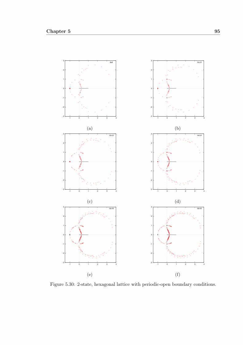
Chapter 5 95

-3

-2

-1

0

1

2

3

-1 0 1 2 3 4

8x8’

(a)

-3

-2

-1

0

1

2

3

-1 0 1 2 3 4

10x10’

(b)

-3

-2

-1

0

1

2

3

-1 0 1 2 3 4

12x12’

(c)

-3

-2

-1

0

1

2

3

-1 0 1 2 3 4

14x14’

(d)

-3

-2

-1

0

1

2

3

-1 0 1 2 3 4

16x16’

(e)

-3

-2

-1

0

1

2

3

-1 0 1 2 3 4

18x18’

(f)

Figure 5.30: 2-state, hexagonal lattice with periodic-open boundary conditions.

96 Chapter 5

For the 2-state hexagonal lattice in Figure 5.30, the zeros in the physical region

form a pattern looking like a bean, especially in the first and forth quadrants. A

visible locus of small circle near the origin and a ‘bean’-like structure starts to appear

in the physical region as we increase the size. At large enough lattice, it is expected

that the distribution will have smooth structures.

For the 3-state case in Figure 5.31, the zeros are still far from the real axis in the

ferro and antiferro regions. However a short arm at the antiferro region seems to

move into the real axis direction. In the 4-state case, the antiferro region in Figure

5.32 also shows a short branch starts to emerge as we increase the lattice size.

We shall see a duality relation between the zeros distributions of triangular lattice

and hexagonal lattice in the next section § 5.4.1. Note that the hexagonal lattice

has polynomial order that is twice the order of polynomial for triangular lattice.

5.4.1 Duality transformation

Here we present the result from the duality transformation (2.11) on the triangular

lattice. The lattice graph duality relation was described in § 2.2. For example,

consider the zeros distributions as shown in Figure 5.33 to Figure 5.36. We can

produce similar zeros distribution for hexagonal lattice using this transformation.

These examples show the implementation of duality transformation on the

available zeros which gives result for its dual case. The result for a bigger hexagonal

lattice can be produced from the triangular lattice; for example the 24×24′ hexagonal

lattice from 12× 12′ triangular lattice.

Chapter 5 97

-3

-2

-1

0

1

2

3

-3 -2 -1 0 1 2 3 4 5

6x6’

(a)

-3

-2

-1

0

1

2

3

-3 -2 -1 0 1 2 3 4 5

8x8’

(b)

-3

-2

-1

0

1

2

3

-3 -2 -1 0 1 2 3 4 5

10x10’

(c)

-3

-2

-1

0

1

2

3

-3 -2 -1 0 1 2 3 4 5

12x12’

(d)


98 Chapter 5

-4

-3

-2

-1

0

1

2

3

4

-3 -2 -1 0 1 2 3 4 5

6x5’

(a)

-4

-3

-2

-1

0

1

2

3

4

-3 -2 -1 0 1 2 3 4 5

8x9’

(b)

-4

-3

-2

-1

0

1

2

3

4

-3 -2 -1 0 1 2 3 4 5

10x13’

(c)


-2

-1.5

-1

-0.5

0

0.5

1

1.5

2

-2 -1.5 -1 -0.5 0 0.5 1 1.5 2

11x11’

(a)

-3

-2

-1

0

1

2

3

-1 0 1 2 3 4

(11x11)

(b)

Figure 5.33: 2-state, duality transformation of 11 by 11 triangular lattice withperiodic-open boundary conditions.

Chapter 5 99

-2

-1.5

-1

-0.5

0

0.5

1

1.5

2

-2 -1.5 -1 -0.5 0 0.5 1 1.5 2

12x12’

(a)

-3

-2

-1

0

1

2

3

-1 0 1 2 3 4

(12x12)

(b)


-2

-1.5

-1

-0.5

0

0.5

1

1.5

2

-2 -1.5 -1 -0.5 0 0.5 1 1.5 2

11x11’

(a)

-3

-2

-1

0

1

2

3

-3 -2 -1 0 1 2 3 4 5

(11x11)

(b)


-2

-1.5

-1

-0.5

0

0.5

1

1.5

2

-2 -1.5 -1 -0.5 0 0.5 1 1.5 2

12x12’

(a)

-3

-2

-1

0

1

2

3

-3 -2 -1 0 1 2 3 4 5

(12x12)

(b)


100 Chapter 5

5.5 On cubic lattice

Here we show the zeros distribution for cubic lattice Q-state Potts models with

Q ≥ 2. Figures 5.37 through 5.42 present the zeros distributions for number of

states Q = 2, 3, 4, 5, 6 on cubic lattice with periodic boundary conditions in x and y

direction and open boundary condition in z direction.

The largest 2-state Potts model on a cubic lattice in this thesis is the size 5 ×

5× 5′ (see Figure 5.38c). We checked the result for big cases for example the zeros

distribution for 5× 5× 5′ and 6× 4× 5′ (see Figure 5.38b) are correct as discuss in

Valani’s thesis [92].

-2

-1

0

1

2

-2 -1 0 1 2

3x3x10’

(a)

-2

-1

0

1

2

-2 -1 0 1 2

3x4x10’

(b)

-2

-1

0

1

2

-2 -1 0 1 2

5x3x10’

(c)

-2

-1

0

1

2

-2 -1 0 1 2

4x4x10’

(d)

Figure 5.37: 2-state, cubic lattice with periodic-periodic-open boundary conditions.

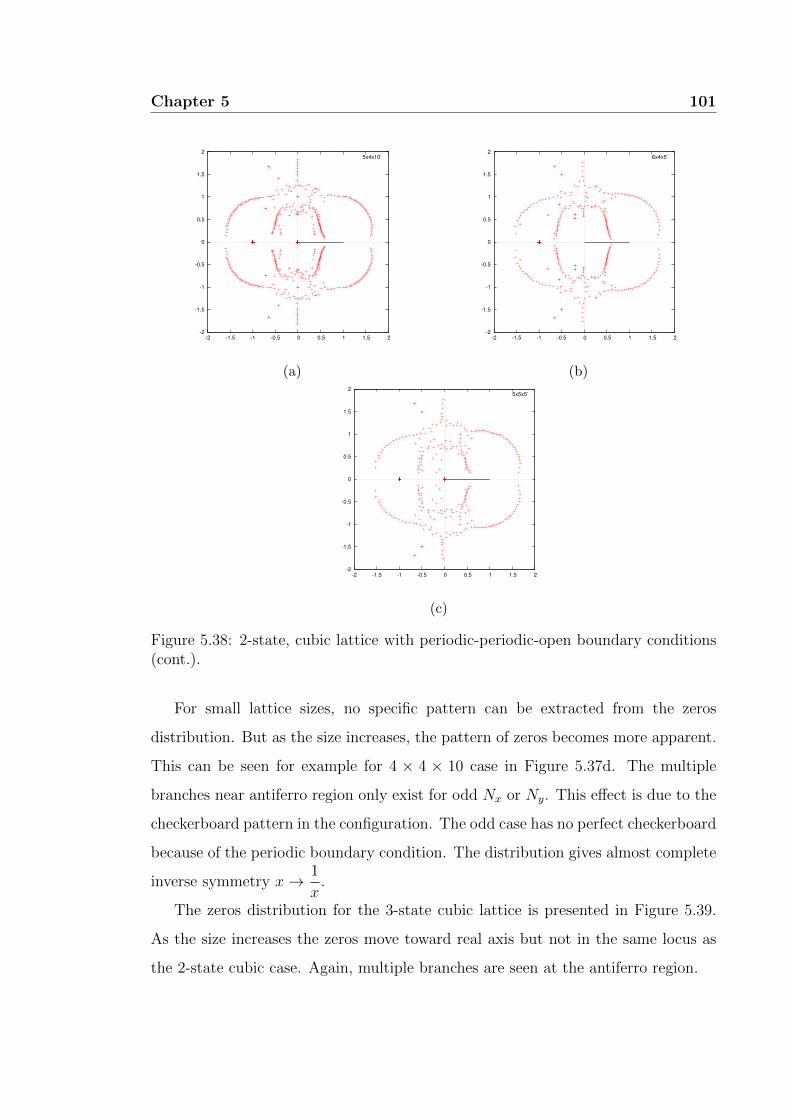
Chapter 5 101

-2

-1.5

-1

-0.5

0

0.5

1

1.5

2

-2 -1.5 -1 -0.5 0 0.5 1 1.5 2

5x4x10’

(a)

-2

-1.5

-1

-0.5

0

0.5

1

1.5

2

-2 -1.5 -1 -0.5 0 0.5 1 1.5 2

6x4x5’

(b)

-2

-1.5

-1

-0.5

0

0.5

1

1.5

2

-2 -1.5 -1 -0.5 0 0.5 1 1.5 2

5x5x5’

(c)

Figure 5.38: 2-state, cubic lattice with periodic-periodic-open boundary conditions(cont.).

For small lattice sizes, no specific pattern can be extracted from the zeros

distribution. But as the size increases, the pattern of zeros becomes more apparent.

This can be seen for example for 4 × 4 × 10 case in Figure 5.37d. The multiple

branches near antiferro region only exist for odd Nx or Ny. This effect is due to the

checkerboard pattern in the configuration. The odd case has no perfect checkerboard

because of the periodic boundary condition. The distribution gives almost complete

inverse symmetry x→ 1

x.

The zeros distribution for the 3-state cubic lattice is presented in Figure 5.39.

As the size increases the zeros move toward real axis but not in the same locus as

the 2-state cubic case. Again, multiple branches are seen at the antiferro region.

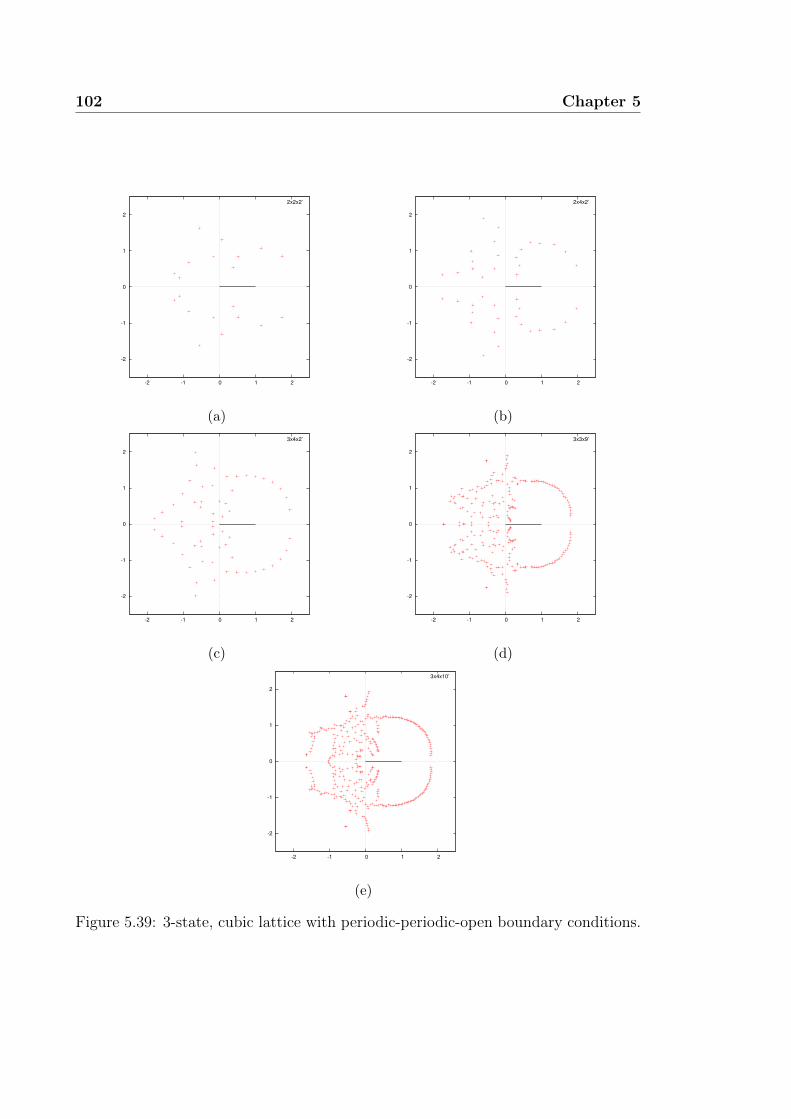
102 Chapter 5

-2

-1

0

1

2

-2 -1 0 1 2

2x2x2’

(a)

-2

-1

0

1

2

-2 -1 0 1 2

2x4x2’

(b)

-2

-1

0

1

2

-2 -1 0 1 2

3x4x2’

(c)

-2

-1

0

1

2

-2 -1 0 1 2

3x3x9’

(d)

-2

-1

0

1

2

-2 -1 0 1 2

3x4x10’

(e)


Chapter 5 103

-2

-1

0

1

2

-2 -1 0 1 2

2x2x3’

(a)

-2

-1

0

1

2

-2 -1 0 1 2

2x2x10’

(b)

-2

-1

0

1

2

-2 -1 0 1 2

2x3x3’

(c)

-2

-1

0

1

2

-2 -1 0 1 2

2x3x10’

(d)

-2

-1

0

1

2

-2 -1 0 1 2

3x3x4’

(e)

-2

-1

0

1

2

-2 -1 0 1 2

3x3x10’

(f)


104 Chapter 5

-2

-1

0

1

2

-2 -1 0 1 2

2x2x3’

(a)

-2

-1

0

1

2

-2 -1 0 1 2

2x2x10’

(b)

-2

-1

0

1

2

-2 -1 0 1 2

2x2x15’

(c)

-2

-1

0

1

2

-2 -1 0 1 2

3x2x4’

(d)

-2

-1

0

1

2

-2 -1 0 1 2

3x2x10’

(e)

-2

-1

0

1

2

-2 -1 0 1 2

3x3x5’

(f)


Chapter 5 105

The zeros distributions for 4-, 5- and 6-state Potts models on cubic lattices are

presented in Figures 5.40, 5.41, and 5.42. The distributions are dominated by the

finite size effect since the pattern is largely changing as the size increases. Although

we can see the zeros move closer to real axis in the ferro region, that is difficult to

conclude exactly for the antiferro part.

-2

-1

0

1

2

-2 -1 0 1 2

2x2x6’

(a)

-2

-1

0

1

2

-2 -1 0 1 2

2x3x6’

(b)

-2

-1

0

1

2

-2 -1 0 1 2

3x2x6’

(c)

-2

-1

0

1

2

-2 -1 0 1 2

3x3x6’

(d)


5.6 On tetragonal and octagonal lattice

The final case that has been considered for the Q-state Potts model is the three-

dimensional cubic lattices with closed packing. Here we consider two types of lattice

106 Chapter 5

with closed packing known as the face-centered cubic lattice and the hexagonal close-

packed lattice. Respectively, we call this two cases by their regular shapes portrayed

in their lattice layer which are the octagonal and tetragonal lattices.

The zeros of the partition function for the 2-state Potts models on tetragonal

lattice is shown in Figure 5.43. For small Nx and Ny, we can see the pattern of

zeros distribution is changing. As the size increases, the pattern develops into more

clear curve towards stability. We can see more symmetries such as x → −x. A

smooth line of zeros approaching the physical axis is also observed. This suggests

the existence of a positive antiferro transition point.

For the tetragonal lattice 3-state case in Figure 5.44, the distribution is

particularly scattered at some part of the non-physical region including the antiferro

region. In ferro region, the zeros getting closer to real axis with dense line. The

3×3×7′ case in Figure 5.44c shows a line emerges in the antiferro region. The finite

size effect is obvious in these distributions portrayed by the zeros that is scattered

in some parts of the plane.

The zeros distribution for the 2-state octagonal lattice is shown in Figure 5.45.

As the size changes, an arm of zeros starts to form and moves closer to the antiferro

region. The behaviour of this zeros is very similar to the tetragonal 2-state case.

Furthermore, the zeros distributions for the 3-state octagonal cases are shown in

Figure 5.46. Again, the similarity with the tetragonal case is observed. The locus

of zeros in the physical region is more stable as compared to the scattered zeros in

the non-physical region.

For the hexagonal close-packed lattice, the vertices are placed in repeated

tetrahedron shape. This arrangement forms another shape of octahedron at some

middle layer of the lattice. This is similar to the face-centered cubic case. For

this reason, although we portrayed them with different regular shape, the zeros

distribution has a similar pattern of distribution. In all these four cases in this

section, the zeros endpoints in ferro region are very close to the real axis.

Chapter 5 107

-2

-1.5

-1

-0.5

0

0.5

1

1.5

2

-2 -1.5 -1 -0.5 0 0.5 1 1.5 2

2x2x7’

(a)

-2

-1.5

-1

-0.5

0

0.5

1

1.5

2

-2 -1.5 -1 -0.5 0 0.5 1 1.5 2

3x2x7’

(b)

-2

-1.5

-1

-0.5

0

0.5

1

1.5

2

-2 -1.5 -1 -0.5 0 0.5 1 1.5 2

3x3x7’

(c)

-2

-1.5

-1

-0.5

0

0.5

1

1.5

2

-2 -1.5 -1 -0.5 0 0.5 1 1.5 2

3x4x7’

(d)

-2

-1.5

-1

-0.5

0

0.5

1

1.5

2

-2 -1.5 -1 -0.5 0 0.5 1 1.5 2

4x4x7’

(e)

Figure 5.43: 2-state, tetragonal lattice with periodic-open boundary conditions.

108 Chapter 5

-2

-1.5

-1

-0.5

0

0.5

1

1.5

2

-2 -1.5 -1 -0.5 0 0.5 1 1.5 2

2x2x7’

(a)

-2

-1.5

-1

-0.5

0

0.5

1

1.5

2

-2 -1.5 -1 -0.5 0 0.5 1 1.5 2

3x2x7’

(b)

-2

-1.5

-1

-0.5

0

0.5

1

1.5

2

-2 -1.5 -1 -0.5 0 0.5 1 1.5 2

3x3x7’

(c)

-2

-1.5

-1

-0.5

0

0.5

1

1.5

2

-2 -1.5 -1 -0.5 0 0.5 1 1.5 2

3x4x7’

(d)

Figure 5.44: 3-state, tetragonal lattice with periodic-open boundary conditions.

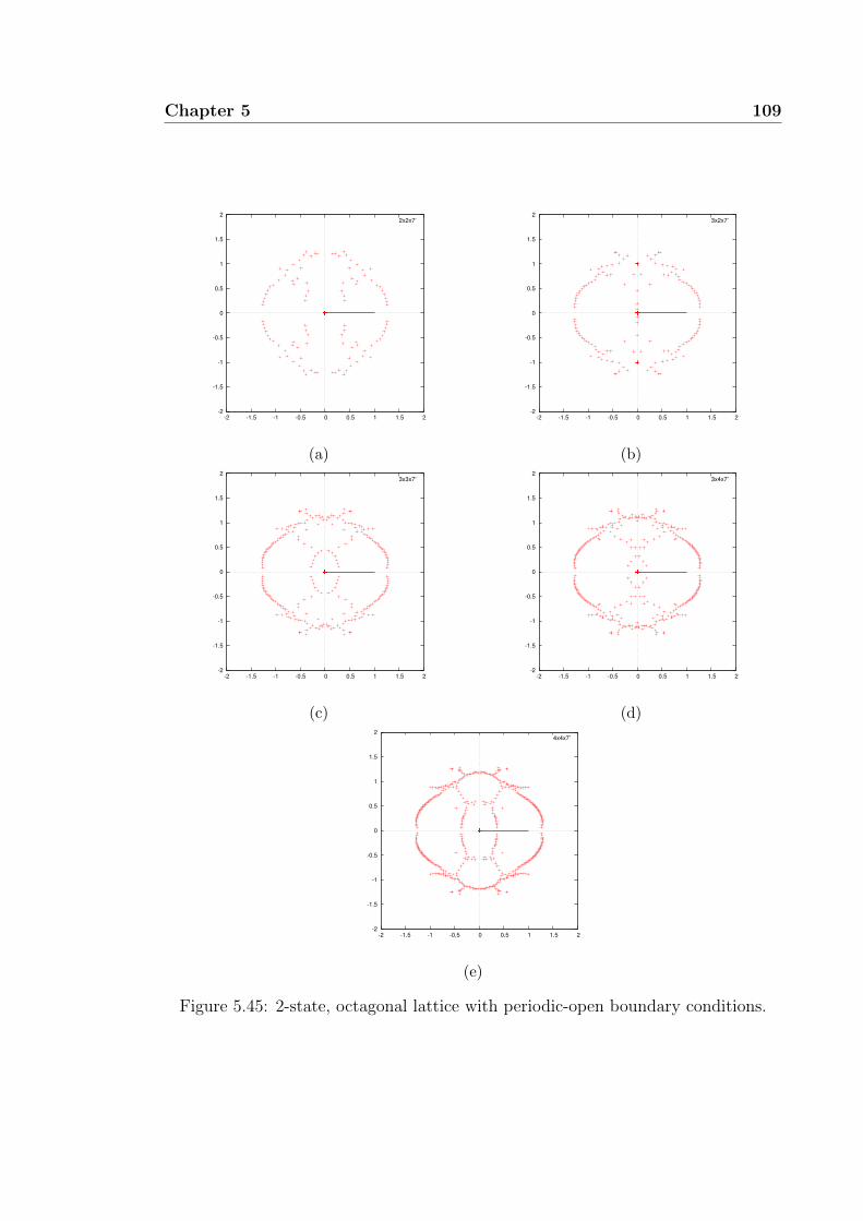
Chapter 5 109

-2

-1.5

-1

-0.5

0

0.5

1

1.5

2

-2 -1.5 -1 -0.5 0 0.5 1 1.5 2

2x2x7’

(a)

-2

-1.5

-1

-0.5

0

0.5

1

1.5

2

-2 -1.5 -1 -0.5 0 0.5 1 1.5 2

3x2x7’

(b)

-2

-1.5

-1

-0.5

0

0.5

1

1.5

2

-2 -1.5 -1 -0.5 0 0.5 1 1.5 2

3x3x7’

(c)

-2

-1.5

-1

-0.5

0

0.5

1

1.5

2

-2 -1.5 -1 -0.5 0 0.5 1 1.5 2

3x4x7’

(d)

-2

-1.5

-1

-0.5

0

0.5

1

1.5

2

-2 -1.5 -1 -0.5 0 0.5 1 1.5 2

4x4x7’

(e)

Figure 5.45: 2-state, octagonal lattice with periodic-open boundary conditions.

110 Chapter 5

-2

-1.5

-1

-0.5

0

0.5

1

1.5

2

-2 -1.5 -1 -0.5 0 0.5 1 1.5 2

2x2x7’

(a)

-2

-1.5

-1

-0.5

0

0.5

1

1.5

2

-2 -1.5 -1 -0.5 0 0.5 1 1.5 2

3x2x7’

(b)

-2

-1.5

-1

-0.5

0

0.5

1

1.5

2

-2 -1.5 -1 -0.5 0 0.5 1 1.5 2

3x3x7’

(c)

-2

-1.5

-1

-0.5

0

0.5

1

1.5

2

-2 -1.5 -1 -0.5 0 0.5 1 1.5 2

3x4x7’

(d)

Figure 5.46: 3-state, octagonal lattice with periodic-open boundary conditions.

5.7 Discussion

We have considered many computable cases of Q-state Potts models on sequence of

crystal lattices from two-dimensional to three-dimensional cases. For each case, we

vary the lattice size and continue to investigate the model for given Q spin directions.

We are interested to investigate the zeros distribution analytic structure particularly

in the physical region.

The locus of points for the 2-state Potts model on square lattice for example

satisfies the result in Chapter 4 i.e. two circles. The exact solution of Ising model

on square lattice by Onsager is the benchmark for checking our computation.

Chapter 5 111

For Q > 3, Q-state Potts models on square lattices show the line of zeros

distribution that is smooth in ferromagnetic region. As the size increases, we can see

the zeros form a nice arc approaching the real axis. However, no visible structure is

manifested in the antiferromagnetic (0, 1)-region. Similar behaviour is observed for

zeros distribution on triangular and hexagonal lattices for Q = 4.

Although the 2-state Potts model on triangular lattice suggests no interesting

structure in the antiferro region, its dual case of hexagonal lattice shows otherwise.

The hexagonal lattice shows the presence of the transition point at ferro and

antiferro regions. Conversely, the 3-state Potts model on triangular lattice has

similar behaviour.

The behaviour of zeros near the positive real axis is understood to be a

corresponding to the behaviour of a physical property near a phase transition [56, 60].

The locus of points formed by the approximation of the zeros distribution near the

limiting size can suggest a particular point on the real axis. The locus cut the real

positive axis at a singular interception point. It corresponds to the critical point

where the system change phases.

For finite lattice, the zeros distribution is always affected by the finite size effect.

For small cases, this effect is dominating the partition function. As the size increases

for a good model, the fuzziness in the distribution (as shown in Figure 5.4) will

eventually stabilise into a limiting pattern of the zeros distribution. From there

a good approximation for the locus of points can be inferred. A stable limiting

zeros distribution is essential to estimate the critical exponents [101] (as explained

in Chapter 7) of phase transition.

The cases that have been considered corresponds to the types of crystal lattice

in solid state [31, 85]. In the next chapter we will consider another model which is

related to Q-state Potts model. The model is called the ZQ-symmetric model.

Chapter 6

The ZQ-symmetric model partition

function zeros

We continue with one more model that is related to the Q-state Potts model called

the ZQ-symmetric model [57, 58]. In this chapter we describe several particular cases

of spin states Q = 5, 6 on square lattice. As before, the Hamiltonian function for

this model is defined and the partition function will then be computed. The energy

relation is studied and the zeros distribution of the partition function is presented

in the complex-eβ plane.

The ZQ-symmetric model is suitable to study a system with many spin directions

especially for Q > 4 and to study a system with possibly multiple phase transitions.

Let Λ = (V,E, f) be a graph. By Definition 1.1.5, the Hamiltonian function of theQ-

state Potts model is defined by H : Ω→ R. For any σ ∈ Ω the Hamiltonian function

H can be written in general function g : Q×Q→ R where (σi, σj) 7→ g(σi, σj), that

is

H(σ) = −J∑


g(σi, σj).

Without loss of generality, the function g can be rescaled to be g′(σi, σj) =

γ1g(σi, σj) + γ2 where γ1, γ2 ∈ R are rescaling factors. The rescaling factor is also

present in the relation (4.1) between Ising and Potts models.

113

114 Chapter 6

6.1 ZQ-symmetric model − definitions

We write the definitions for the ZQ-symmetric model in this section. The idea of

this model is that the spin directions are drawn in a clock-like circle. Each spin

direction is associated with an interaction energy of one spin relative to another

spin, written outside of the circle. As we move any pair of spin direction with fixed

angle around the clock, the energy difference will always remains the same. This

property represents the symmetry for this model.

1

23

1

γ1γ2

(a)

1

23

1

γ1γ2

(b)

1

23

1

γ1γ2

(c)

Figure 6.1: The interaction of a spin relative to spin 1 represented by a pair of arrow.

We restrict our study into the case with positive energy value. Given graph

Λ = (V,E, f), let the space of spin configuration for the ZQ-symmetric model be

similar to the Q-state Potts model. A function σ : V → Q = 1, 2, ..., Q is a spin

configuration for a ZQ-symmetric model.

For any microstate σ ∈ Ω we define the Hamiltonian function of the ZQ-

symmetric model below.

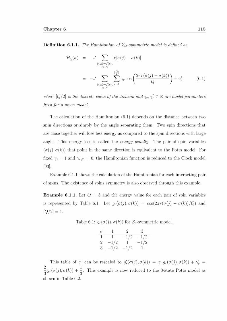
Chapter 6 115

Definition 6.1.1. The Hamiltonian of ZQ-symmetric model is defined as

Hχ(σ) = −J∑

〈j,k〉=f(e),e∈E

χ[σ(j)− σ(k)]

= −J∑


[Q2

]∑r=1

γr cos

(2πr(σ(j)− σ(k))

Q

)+ γ′r (6.1)

where [Q/2] is the discrete value of the division and γr, γ′r ∈ R are model parameters

fixed for a given model.

The calculation of the Hamiltonian (6.1) depends on the distance between two

spin directions or simply by the angle separating them. Two spin directions that

are close together will lose less energy as compared to the spin directions with large

angle. This energy loss is called the energy penalty. The pair of spin variables

(σ(j), σ(k)) that point in the same direction is equivalent to the Potts model. For

fixed γ1 = 1 and γr 6=1 = 0, the Hamiltonian function is reduced to the Clock model

[93].

Example 6.1.1 shows the calculation of the Hamiltonian for each interacting pair

of spins. The existence of spins symmetry is also observed through this example.

Example 6.1.1. Let Q = 3 and the energy value for each pair of spin variables

is represented by Table 6.1. Let gr(σ(j), σ(k)) = cos(2πr(σ(j) − σ(k))/Q) and

[Q/2] = 1.

Table 6.1: gr(σ(j), σ(k)) for Z3-symmetric model.

σ 1 2 31 1 −1/2 −1/22 −1/2 1 −1/23 −1/2 −1/2 1

This table of gr can be rescaled to g′r(σ(j), σ(k)) = γr gr(σ(j), σ(k)) + γ′r =2

3gr(σ(j), σ(k)) +

1

3. This example is now reduced to the 3-state Potts model as

shown in Table 6.2.

116 Chapter 6

Table 6.2: g′r(σ(j), σ(k)) for Z3-symmetric model.

σ 1 2 31 1 0 02 0 1 03 0 0 1

For the Potts model, a pair of nearest neighbour vertices pointing in the same

direction gives an energy value 1 and 0 otherwise. This choice of value corresponds

to a large energy penalty. For the ZQ-symmetric model, the energy value is between

0 and 1. The cases with Q = 2, 3, and 4 are covered by the Potts and Ising models.

The interesting case for this model is thus given by Q > 4.

Figures 6.1 and 6.2 give illustrations of the following statement. The energy

values of the model can be written as a list of possible choices of energy χ =

(χ[0], χ[1], χ[2], ...) ∈ [0, 1]. The χ is a list of energy between Q different spin

directions. The arrows in the clock correspond to the spin directions of one spin

relative to spin 1. The list is arranged in the order of increasing angles relative to

one spin direction.

We consider the value of energy on the clock that has reflection symmetry (see

Figure 6.2). We write the energy list up to half of the total spin direction i.e.

χ = (χ[0], χ[1], ..., χ[n]) where n =Q

2if Q is even and n =

Q− 1

2if Q is odd. Let θ

be the angle between 2 spin directions. The energy value 1 corresponds to cos θ = 1

(i.e. θ = 0) and energy value 0 corresponds to cos θ = 0 (i.e. θ = π/2).

In all cases, we let the first element χ[0] = 1 and the last element χ[n] = 0.

Figure 6.2 illustrates the arrangement of this energy list for Q = 4, 5 and 6 where

χ = (1, χ[1] = γ1, χ[2] = γ2, ...). The χ = (1, γ1, 0) corresponds to the case with spin

state Q = 4, 5 and the χ = (1, γ1, γ2, 0) corresponded to Q = 6.

Similar to the Potts model, the number of calculations can be reduced by using

symmetry. For this model we are able to translate all the spin directions around the

clock.

The energy list χ can be rescaled into discrete number by multiplying with an

Chapter 6 117

1

2

3

1

γ1

0

4γ1

(a)

1

2

3

1

γ1

0

4

5

γ1

0

(b)

1

2

3

1

γ1

0

45

γ1

γ2γ2

6

(c)

Figure 6.2: The illustration of energy list with: (a) χa = (1, γ1, 0), (b) χb = (1, γ1, 0),and (c) χc = (1, γ1, γ2, 0).

appropriate integer, i.e. χ = Cχ where C ∈ N. The energy value can be chosen in

this range 0 ≤ χ[i] ≤ C. See Example 6.1.2.

Example 6.1.2. See Figure 6.3. Suppose the spin state has Q = 4. The energy list

χ = (1, 2/3, 0) corresponds to

g(σ1, σ1) = 1,

g(σ1, σ2) = 2/3,

g(σ1, σ3) = 0,

g(σ1, σ4) = 2/3.

Without loss of generality, the new energy list is χ = 3χ = (3, 2, 0) which

118 Chapter 6

1

2

3

1

42/3 2/3

0

1

2

3

3

4

2 2

0

Figure 6.3: The illustration of Z4-symmetric model with energy value χ = (1, 2/3, 0)(left) and χ = 3χ = (3, 2, 0) (right).

corresponds to

g′(σ1, σ1) = 3,

g′(σ1, σ2) = 2,

cg′(σ1, σ3) = 0,

g′(σ1, σ4) = 2.

To show how the energy list χ is related to Hamiltonian Hχ, we give example

for Q = 4 and Q = 6.

Example 6.1.3. Let Q = 4. For χ = (χ[0], χ[1], χ[2]) = (2, 1, 0) the Hamiltonian is

given by

H(2,1,0)(σ) = −J∑


χ[σ(j)− σ(k)]

= −J∑


1 + cos

(π(σ(j)− σ(k))

2

)(6.2)

where γ1 = γ′1 = 1 and γ2 = γ′2 = 0.

Example 6.1.4. Let Q = 6. For χ = (χ[0], χ[1], χ[2], χ[3]) = (2, 1, 0, 0) the

Chapter 6 119

Hamiltonian is given by

H(2,1,0,0)(σ) = −J∑


χ[σ(j)− σ(k)]

= −J∑


2

3+ cos

(π(σ(j)− σ(k))

3

)

+1

3cos

(2π(σ(j)− σ(k))

3

)(6.3)

where γ1 = 1, γ′1 = 2/3, γ2 = 1/3, and γ′2 = γ3 = γ′3 = 0.

The partition function for the ZQ-symmetric model on Λ is given by (1.1), i.e.

Z =∑σ∈Ω

exp(−βHχ(σ))

where Hχ is as in Definition 6.1.1.

Let N,M ∈ N. We consider a ZQ-symmetric model on a square lattice of N by

M size. We restrict our study of partition function for the case of mixed boundary

condition i.e. periodic in vertical direction and open in horizontal direction. We

denote the energy penalty between two spins in the energy list χ by an energy step

notation given by value (χ[1]− χ[0], χ[2]− χ[1], ...)-step. We will use this notation

later for comparing the χ values.

6.2 The zeros distribution on square lattice

Here we present the result of the zeros distribution of the partition function for Z5-

and Z6-symmetric models.

The figures of zeros distribution are arranged in increasing lattice sizes for

respective χ value. Table 6.3 shows all the cases under study for Z5- and Z6-

symmetric models in this chapter.

Our hypothesis is that the emergence of circular arcs in the physical region

can be used to determine the number of phase transitions for a physical system

120 Chapter 6

[58]. Multiple arcs of zeros approaching the real axis correspond to the existence of

multiple phase transitions.

Table 6.3: The Z5- and Z6-symmetric models with arbitrary χ. New results arehighlighted grey.

χ 5x5’ 6x6’ 6x7’ 7x7’ 8x8’ 9x9’

Q=5

(2,1,0) X X X X X X(3,1,0) X X X X X X(3,2,0) X X X X X X(4,1,0) X X X X X X(4,3,0) X X X X X X(5,3,0) X X X X X(5,4,0) X X X X X(6,1,0) X X X X X(6,5,0) X X X X X

Q=6

(2,1,0,0) X X X X X(2,1,1,0) X X X X X(3,1,0,0) X X X X X(3,2,0,0) X X X X X(3,2,1,0) X X X X X

6.2.1 5-state: Z5-symmetric

Consider the Z5-symmetric model on finite size square lattice with some energy

value χ. The study on 6 by 7 square lattice which was described by Martin [58] is

our reference for checking and comparison.

Figure 6.4 shows the zeros distribution of Z5-symmetric model with χ = (2, 1, 0).

The χ value has a (1,1)-step energy penalty. In the antiferro region, two behaviours

are observed. For even N , few lines indicated in Figure 6.4 are merged forming

single curve move closer to the real axis. As the lattice size increases, a clear curve

is observed. For odd N , we see multiple lines are approaching the antiferro region.

In the ferro region, as the number of vertices N increases, the zeros show the

emergence of multiple lines near the real axis. It is not clear either the lines will

remain or merge to form a thin arm suggesting single phase transition. The case

of χ = (2, 1, 0) for 6 by 7 square lattice has been described by Martin [58] in the

Chapter 6 121

-2

-1

0

1

2

-2 -1 0 1 2

5x5’

(a)

-2

-1

0

1

2

-2 -1 0 1 2

6x6’

(b)

-2

-1

0

1

2

-2 -1 0 1 2

6x7’

(c)

-2

-1

0

1

2

-2 -1 0 1 2

7x7’

(d)

-2

-1

0

1

2

-2 -1 0 1 2

8x8’

(e)

-2

-1

0

1

2

-2 -1 0 1 2

9x9’

(f)

Figure 6.4: Zeros distribution for χ = (2, 1, 0) 5-state model.

122 Chapter 6

complex-e−β plane. He shows that this case has only 1 transition in the ferro region.

That case is just the inverse version of the one presented in Figure 6.4c.

-2

-1

0

1

2

-2 -1 0 1 2

5x5’

(a)

-2

-1

0

1

2

-2 -1 0 1 2

6x6’

(b)

-2

-1

0

1

2

-2 -1 0 1 2

6x7’

(c)

-2

-1

0

1

2

-2 -1 0 1 2

7x7’

(d)

-2

-1

0

1

2

-2 -1 0 1 2

8x8’

(e)

-2

-1

0

1

2

-2 -1 0 1 2

9x9’

(f)


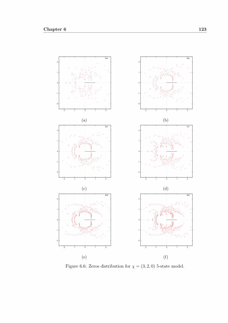
Chapter 6 123

-2

-1

0

1

2

-2 -1 0 1 2

5x5’

(a)

-2

-1

0

1

2

-2 -1 0 1 2

6x6’

(b)

-2

-1

0

1

2

-2 -1 0 1 2

6x7’

(c)

-2

-1

0

1

2

-2 -1 0 1 2

7x7’

(d)

-2

-1

0

1

2

-2 -1 0 1 2

8x8’

(e)

-2

-1

0

1

2

-2 -1 0 1 2

9x9’

(f)


124 Chapter 6

Next, we present the distribution of χ = (3, 1, 0) in Figure 6.5 and χ = (3, 2, 0)

in Figure 6.6. Both figures are related to each other through their number of steps

of the energy penalty. The χ = (3, 2, 0) has (1, 2) energy step. This step is the

inverse steps of χ = (3, 1, 0) which has (2, 1) energy step.

For χ = (3, 1, 0) there exist single line of zeros in ferro region approaching the

real axis. The antiferro region shows the emergence of two lines but it is not very

clear either the lines will remain or merge at the thermodynamic limit.

For χ = (3, 2, 0) in Figure 6.6, there exist several distinct lines approaching the

real axis. We claim that at the limit two circular arcs will approach the real axis in

the ferro region. This observation is obvious based on the increasing number of zeros

in this region. In the antiferro region, we can see that as the lattice size increases,

a thick single band is approaching the real axis. The emergence of two lines in odd

case is just due to the boundary effect. If the antiferromagnetic phase transition

exists, this case has only a single transition given by the single line of dense zeros

near the real axis.

A further comparison is made between Figures 6.7 and 6.8. Both cases are related

to each other through their number of steps (energy penalty) that is (3, 1)-step for

χ = (4, 1, 0) and (1, 3)-step for χ = (4, 3, 0). The ferro region in Figure 6.7 presents

the existence of single limiting critical point. On the other hand, there exist two lines

approaching the real axis in antiferro region. This behaviour suggests the antiferro

region may have single or double transition point in the limit N →∞.

Conversely, the case shown in the Figure 6.8 is opposite to the one in Figure 6.7.

The antiferro region is expected to give single transition whereas the ferro region

shows a strong possibility of multiple transition points as N →∞.

Figure 6.9 shows the distribution of zeros for χ = (5, 3, 0) with energy penalty

(2, 3)-step. Although the lattice size is considered to be small, we can already see

the expected number of critical points for this system. At N = 6, the Figure 6.9b

suggests the possibility of multiple transition at the ferro region and single transition

at the antiferro region. The smooth line in Figure 6.9b gives a clue of boundary

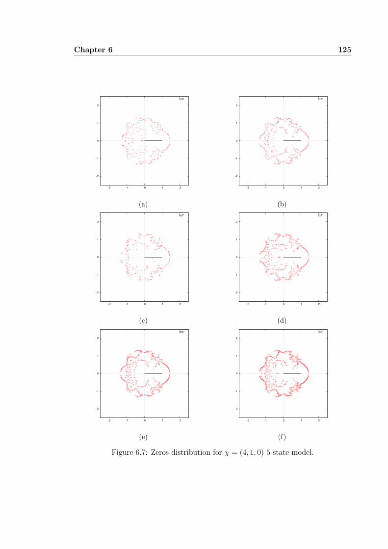
Chapter 6 125

-2

-1

0

1

2

-2 -1 0 1 2

5x5’

(a)

-2

-1

0

1

2

-2 -1 0 1 2

6x6’

(b)

-2

-1

0

1

2

-2 -1 0 1 2

6x7’

(c)

-2

-1

0

1

2

-2 -1 0 1 2

7x7’

(d)

-2

-1

0

1

2

-2 -1 0 1 2

8x8’

(e)

-2

-1

0

1

2

-2 -1 0 1 2

9x9’

(f)


126 Chapter 6

-2

-1

0

1

2

-2 -1 0 1 2

5x5’

(a)

-2

-1

0

1

2

-2 -1 0 1 2

6x6’

(b)

-2

-1

0

1

2

-2 -1 0 1 2

6x7’

(c)

-2

-1

0

1

2

-2 -1 0 1 2

7x7’

(d)

-2

-1

0

1

2

-2 -1 0 1 2

8x8’

(e)

-2

-1

0

1

2

-2 -1 0 1 2

9x9’

(f)


Chapter 6 127

-2

-1.5

-1

-0.5

0

0.5

1

1.5

2

-2 -1.5 -1 -0.5 0 0.5 1 1.5 2

5x5’

(a)

-2

-1.5

-1

-0.5

0

0.5

1

1.5

2

-2 -1.5 -1 -0.5 0 0.5 1 1.5 2

6x6’

(b)

-2

-1.5

-1

-0.5

0

0.5

1

1.5

2

-2 -1.5 -1 -0.5 0 0.5 1 1.5 2

6x7’

(c)

-2

-1.5

-1

-0.5

0

0.5

1

1.5

2

-2 -1.5 -1 -0.5 0 0.5 1 1.5 2

7x7’

(d)

-2

-1.5

-1

-0.5

0

0.5

1

1.5

2

-2 -1.5 -1 -0.5 0 0.5 1 1.5 2

7x9’

(e)

-2

-1.5

-1

-0.5

0

0.5

1

1.5

2

-2 -1.5 -1 -0.5 0 0.5 1 1.5 2

8x8’

(f)


128 Chapter 6

-2

-1.5

-1

-0.5

0

0.5

1

1.5

2

-2 -1 0 1 2

5x5’

(a)

-2

-1.5

-1

-0.5

0

0.5

1

1.5

2

-2.5 -2 -1.5 -1 -0.5 0 0.5 1 1.5 2 2.5

6x6’

(b)

-2

-1.5

-1

-0.5

0

0.5

1

1.5

2

-2 -1 0 1 2

6x7’

(c)

-2

-1.5

-1

-0.5

0

0.5

1

1.5

2

-2 -1 0 1 2

7x7’

(d)

-2

-1.5

-1

-0.5

0

0.5

1

1.5

2

-2 -1 0 1 2

7x9’

(e)

-2

-1.5

-1

-0.5

0

0.5

1

1.5

2

-2 -1 0 1 2

8x8’

(f)


Chapter 6 129

-2

-1.5

-1

-0.5

0

0.5

1

1.5

2

-2 -1.5 -1 -0.5 0 0.5 1 1.5 2

5x5’

(a)

-2

-1.5

-1

-0.5

0

0.5

1

1.5

2

-2 -1.5 -1 -0.5 0 0.5 1 1.5 2

6x6’

(b)

-2

-1.5

-1

-0.5

0

0.5

1

1.5

2

-2 -1.5 -1 -0.5 0 0.5 1 1.5 2

6x7’

(c)

-2

-1.5

-1

-0.5

0

0.5

1

1.5

2

-2 -1.5 -1 -0.5 0 0.5 1 1.5 2

7x7’

(d)

-2

-1.5

-1

-0.5

0

0.5

1

1.5

2

-2 -1.5 -1 -0.5 0 0.5 1 1.5 2

7x9’

(e)

-2

-1.5

-1

-0.5

0

0.5

1

1.5

2

-2 -1.5 -1 -0.5 0 0.5 1 1.5 2

8x8’

(f)


130 Chapter 6

-2

-1.5

-1

-0.5

0

0.5

1

1.5

2

-2 -1 0 1 2

5x5’

(a)

-2

-1.5

-1

-0.5

0

0.5

1

1.5

2

-2.5 -2 -1.5 -1 -0.5 0 0.5 1 1.5 2 2.5

6x6’

(b)

-2

-1.5

-1

-0.5

0

0.5

1

1.5

2

-2 -1 0 1 2

6x7’

(c)

-2

-1.5

-1

-0.5

0

0.5

1

1.5

2

-2 -1 0 1 2

7x7’

(d)

-2

-1.5

-1

-0.5

0

0.5

1

1.5

2

-2 -1 0 1 2

7x9’

(e)

-2

-1.5

-1

-0.5

0

0.5

1

1.5

2

-2 -1 0 1 2

8x8’

(f)


Chapter 6 131

effect in the odd N case; for example at N = 7. It is evidenced from this structure

that the number of transitions is two in ferro region and one in antiferro region.

Figures 6.11 and 6.12 are more examples with inverse relation through the

number of penalty steps. The case χ = (6, 1, 0) in Figure 6.11 can only suggest

the existence of single transition in the ferro region while it is not clear for the

antiferro part. Interestingly for χ = (6, 5, 0) in Figure 6.12, the distribution in

the ferro region shows multiple lines approaching the real axis. This ferro region

corresponds to the antiferro part of χ = (6, 1, 0).

This result is interesting because at previous example between χ = (3, 1, 0) and

χ = (3, 2, 0), the number of transitions is also opposite to each other. We can

investigate two cases that is related by the energy penalty step by considering only

one of the cases.

6.2.2 6-state: Z6-symmetric

We continue with square lattice of the Z6-symmetric model. Refer Table 6.3. Similar

to the Z5-symmetric case, the study on 6 by 7 square lattice was described by Martin

[58].

For 6-state model, the degree of partition function polynomial increases rapidly

due to the higher number of states (Q = 6) as the lattice size increases. Thus only

small cases are available due to computing limitation. We consider the study of

6-state model on square lattice up to 8 by 8 lattice size, i.e. |V | = 64.

Figure 6.13 presents the zeros distribution for χ = (2, 1, 0, 0) with (1, 1, 0)-step.

The zeros distribution in the ferro and antiferro regions indicates that there is only

a single transition point in each region. For even N , the zeros distribution shows

smoother and visible pattern than those for odd N .

Interestingly, for the case χ = (2, 1, 1, 0) with (1, 0, 0)-step, the zeros shown in

Figure 6.14 have a stable pattern approaching the real axis as the size increases.

Both physical regions have clear behaviour of a smooth line indicating the existence

of single transition.

132 Chapter 6

-2

-1

0

1

2

-2 -1 0 1 2

5x5’

(a)

-2

-1

0

1

2

-2 -1 0 1 2

6x6’

(b)

-2

-1

0

1

2

-2 -1 0 1 2

6x7’

(c)

-2

-1

0

1

2

-2 -1 0 1 2

7x7’

(d)

-2

-1

0

1

2

-2 -1 0 1 2

8x8’

(e)

Figure 6.13: Zeros distribution for χ = (2, 1, 0, 0) 6-state model.

Chapter 6 133

-2

-1

0

1

2

-3 -2 -1 0 1 2 3

5x5’

(a)

-2

-1

0

1

2

-3 -2 -1 0 1 2 3

6x6’

(b)

-2

-1

0

1

2

-3 -2 -1 0 1 2 3

6x7’

(c)

-2

-1

0

1

2

-3 -2 -1 0 1 2 3

7x7’

(d)

-2

-1

0

1

2

-3 -2 -1 0 1 2 3

8x8’

(e)


134 Chapter 6

-2

-1

0

1

2

-2 -1 0 1 2

5x5’

(a)

-2

-1

0

1

2

-2 -1 0 1 2

6x6’

(b)

-2

-1

0

1

2

-2 -1 0 1 2

6x7’

(c)

-2

-1

0

1

2

-2 -1 0 1 2

7x7’

(d)

-2

-1

0

1

2

-2 -1 0 1 2

8x8’

(e)


Chapter 6 135

-2

-1

0

1

2

-2 -1 0 1 2

5x5’

(a)

-2

-1

0

1

2

-2 -1 0 1 2

6x6’

(b)

-2

-1

0

1

2

-2 -1 0 1 2

6x7’

(c)

-2

-1

0

1

2

-2 -1 0 1 2

7x7’

(d)

-2

-1

0

1

2

-2 -1 0 1 2

8x8’

(e)


136 Chapter 6

-2

-1

0

1

2

-2 -1 0 1 2

5x5’

(a)

-2

-1

0

1

2

-2 -1 0 1 2

6x6’

(b)

-2

-1

0

1

2

-2 -1 0 1 2

6x7’

(c)

-2

-1

0

1

2

-2 -1 0 1 2

7x7’

(d)

-2

-1

0

1

2

-2 -1 0 1 2

8x8’

(e)


Chapter 6 137

To proceed, the next case is shown in Figure 6.15 with χ = (3, 1, 0, 0) where the

energy penalty is in the (2, 1, 0)-step. Here there is a branch of dense points in the

antiferro region getting closer to real axis. It is expected that the ferro and antiferro

regions have only a single transition point in the limit.

The distribution for χ = (3, 2, 0, 0) is illustrated in Figure 6.16. In this case there

exist two possible transition points in the ferro region and only single point in the

antiferro region.

The final case of 6-state for χ = (3, 2, 1, 0) is shown in Figure 6.17. The

ferro region suggests the existence of two transition points at thermodynamic limit.

However for the antiferro region, it is hard to infer the number of transitions. The

big arm branch in this region has two brief lines emanating from the arm. Two

possibilities can be predicted. First the two small lines will eventually merge at a

point close to real axis. Second the small lines will go further to real axis separately.

The first statement suggests the existence of single transition point. The latter

means the existence of two transition points.

So far we only describe the figures based on our observation directly on the

distribution structure in all the complex-eβ plane. In the next section, further

discussion of the result and more comparison among these cases will continue.

6.3 Discussion

We highlight few more details for comparison among the zeros distributions of Z5-

and Z6-symmetric models in this section.

In general, the distribution is affected by the boundary condition and the finite

size effect especially in the odd N case. In this case, we can see for example in

Figure 6.12d that some of the zeros in the antiferro region are not nicely distributed

on a smooth line.

As the lattice size increases, we can distinguish the zeros movement towards the

real axis for even and odd N . Interestingly, the zeros movement in the ferro region

138 Chapter 6

looks more stable as compared to the antiferro region. The zeros in the antiferro

region for even N shows a smoother line than the odd N near the real axis.

The results for the Z5- and Z6-symmetric models show the emergence of visible

lines as the number of zeros increases. As the lattice size increases, more zeros in

the distribution form some branches in physical and non-physical region. A visible

pattern of distribution can be seen where the zeros get closer to the real axis. At

thermodynamic limit N →∞, the zeros is expected to touch the real line at critical

point of the phase transition.

Consider one layer of a square lattice with vertical spins σ(js) = k (mod Q) ≡ s

with s = 0, 1, 2, · · · , N − 1. This is one of the antiferromagnetic ground state where

the vertices have spins with multiple of Q repeated in the vertical direction. The

number of ways for a system to be in this ground states is high. However, the most

probable kind of ground state is still an open question.

From all the figures in this chapter, we can see that the transition points are

vary based on the energy list χ. The choice of χ value differs by their energy step

relative to the first element of the energy list. We call this the first energy followed

by second, third and so on. Denotes the energy step as αi where index i determine

the sequence of the energy difference.

Figures 6.18 to 6.19 show the zeros distributions of the Z5-symmetric model on

6 by 6 square lattices with all their considered χ values. The χ with an energy step

α1 < α2 gives two arcs of zeros distribution in ferro region. This difference shows the

existence of more than one transition point in the limit. The case with α1 > α2 has

only single arc in this region which implies single transition point. For the α1 = α2

like the case of χ = (2, 1, 0), this case has either one or two transition points. The

exact number of transitions for this case is not clear. From this example, we may

predict the number of transitions based on the energy penalty step. This problem

is still open. We need bigger lattice to provide more evidence for this idea.

The Z5- and Z6-symmetric model zeros distributions show the existence of line

of zeros in the antiferro region. This observation does not exist for the 5- and 6-state

Chapter 6 139

Potts model on square lattice (as discussed in § 5.3).

-2

-1

0

1

2

-2 -1 0 1 2

6x6’

(a) χ = (2, 1, 0)

-2

-1

0

1

2

-2 -1 0 1 2

6x6’

(b) χ = (3, 1, 0)

-2

-1

0

1

2

-2 -1 0 1 2

6x6’

(c) χ = (3, 2, 0)

-2

-1

0

1

2

-2 -1 0 1 2

6x6’

(d) χ = (4, 1, 0)

-2

-1

0

1

2

-2 -1 0 1 2

6x6’

(e) χ = (4, 3, 0)

Figure 6.18: Zeros distribution for several χ of 6 by 6 on square lattice.

140 Chapter 6

-2

-1.5

-1

-0.5

0

0.5

1

1.5

2

-2 -1.5 -1 -0.5 0 0.5 1 1.5 2

6x6’

(a) χ = (5, 3, 0)

-2

-1.5

-1

-0.5

0

0.5

1

1.5

2

-2.5 -2 -1.5 -1 -0.5 0 0.5 1 1.5 2 2.5

6x6’

(b) χ = (5, 4, 0)

-2

-1.5

-1

-0.5

0

0.5

1

1.5

2

-2 -1.5 -1 -0.5 0 0.5 1 1.5 2

6x6’

(c) χ = (6, 1, 0)

-2

-1.5

-1

-0.5

0

0.5

1

1.5

2

-2.5 -2 -1.5 -1 -0.5 0 0.5 1 1.5 2 2.5

6x6’

(d) χ = (6, 5, 0)

Figure 6.19: Zeros distribution for several χ of 6 by 6 on square lattice (cont.).

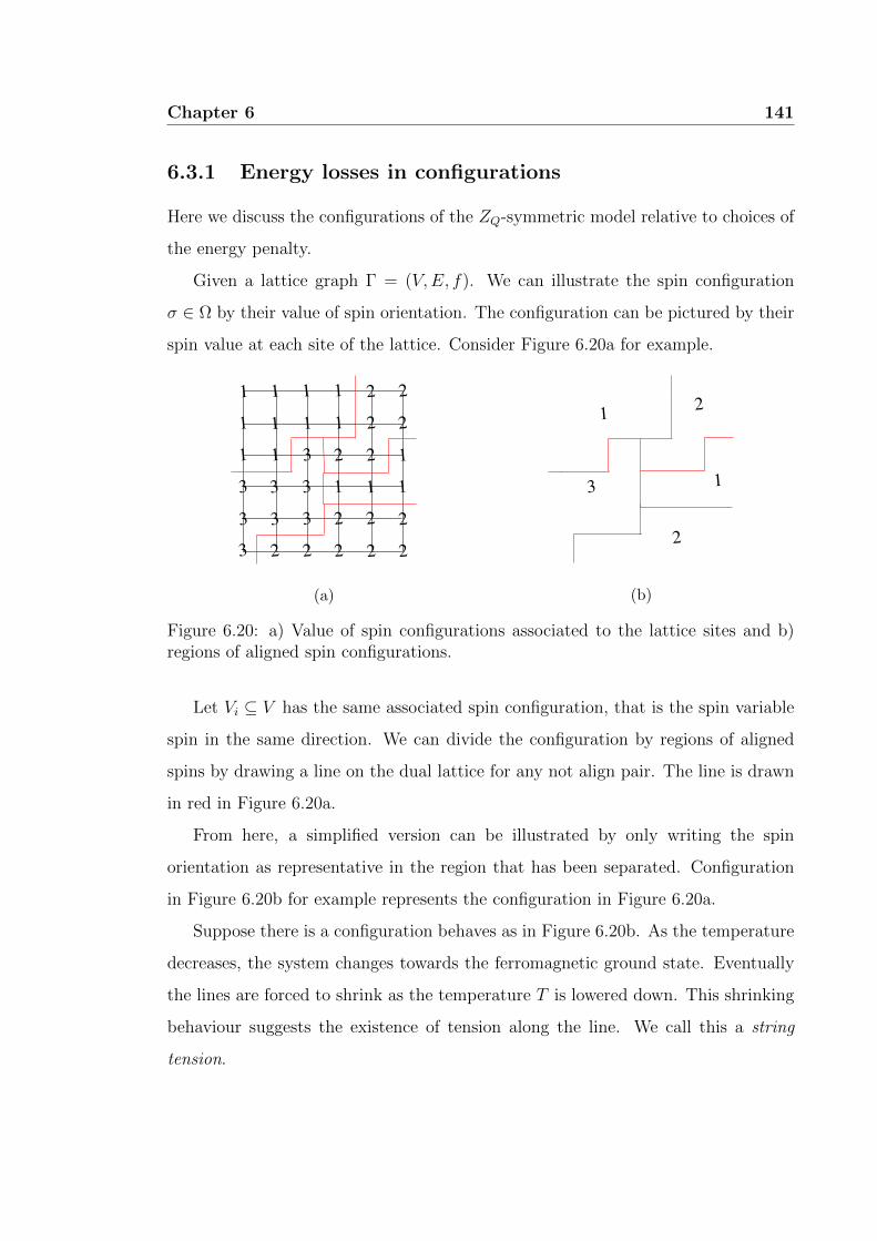
Chapter 6 141

6.3.1 Energy losses in configurations

Here we discuss the configurations of the ZQ-symmetric model relative to choices of

the energy penalty.

Given a lattice graph Γ = (V,E, f). We can illustrate the spin configuration

σ ∈ Ω by their value of spin orientation. The configuration can be pictured by their

spin value at each site of the lattice. Consider Figure 6.20a for example.

1 1 1 1 2 2

221111

1 1 3 2 2 1

3 3 3 1 1 1

3 3 3 2 2 2

3 2 2 2 2 2

(a)

3

21

1

2

(b)

Figure 6.20: a) Value of spin configurations associated to the lattice sites and b)regions of aligned spin configurations.

Let Vi ⊆ V has the same associated spin configuration, that is the spin variable

spin in the same direction. We can divide the configuration by regions of aligned

spins by drawing a line on the dual lattice for any not align pair. The line is drawn

in red in Figure 6.20a.

From here, a simplified version can be illustrated by only writing the spin

orientation as representative in the region that has been separated. Configuration

in Figure 6.20b for example represents the configuration in Figure 6.20a.

Suppose there is a configuration behaves as in Figure 6.20b. As the temperature

decreases, the system changes towards the ferromagnetic ground state. Eventually

the lines are forced to shrink as the temperature T is lowered down. This shrinking

behaviour suggests the existence of tension along the line. We call this a string

tension.

142 Chapter 6

For the study on the Potts model, the line separating the spin region gives no

significant difference for the study. It assigned a 0 value for any pair of spin variables

with different spin. However this is different for the ZQ-symmetric model. The line

separation shows significant correspondence to the total energy of the system.

For neighbouring vertices with points to directions close to each other (small

degree), the configuration state is almost stable at the ground state. The energy

varies according to the choices of χ.

Refering to Figures 6.20 and 6.21, some configurations may also have a point

of intersection between the line separations. This intersection is called vortex. The

length of the line separation corresponds to the value of the total energy penalty.

1

2

3

3

2222 2 22 22 2 2

2

2

2

2

21

1

1

1

1

1

1

1

1

1

1

1

1 1 1 3 3 3 3 3 3 3 3 3

3

3

3

3

Figure 6.21: A configuration with fixed boundary condition.

Here we observe that the first kind of disordered states is the one with small

variation. Many microstates have small energy penalty. As the temperature varies,

the first phase corresponds to the kind of ordered state with slow varying angle.

Then it is followed by a transition to another phase (small disorder) and then to a

completely disordered state.

The largest magnitude of the Hamiltonian represents the ground state where

the free energy is at minimum. For a configuration state represented by some line

separation, one can determine the Hamiltonian energy of that particular state. Since

the length of the line corresponds to the value of the energy penalty, therefore the

ground state can be described by the shortest length of line separation. The shortest

line means lowest energy penalty.

Chapter 6 143

The ZQ-symmetric model is the final model we have considered in this thesis.

We give evidence that the distribution of this model for specific value of χ may

exhibit multiple transitional phases. The analytic structure of the zeros distribution

highlights the possibility of this occurrence.

Chapter 7 will continue with the analysis of the zeros distribution particularly

related to the value of specific heat critical exponent. This is then followed by the

analysis for multiple phases in Chapter 8.

Chapter 7

Analysis on zeros density of

partition function

Here we study the relation between the specific heat critical exponent [58, 101] and

the zero distribution of the partition function.

The hypothesis is that the exponent can be computed from (sufficiently large)

finite lattice distributions. (The hypothesis was proposed in [55], but at that time

the accessible lattices were too small for testing.)

We test this first using our methods on the Onsager/Kaufman Ising solution,

where we both have access to all the finite partition functions Z, and also know

the exact exponent. Then we apply our methods to the square lattice 3-state Potts

model (which is not integrable, but for which the folklore is certain that α = 1/3

[101]).

Suppose we heat ice. Assume that the heat is transferred at the same rate. It

takes some time before the ice turns to water completely. The existence of two

phases of solid ice and liquid water show the process of phase transition. This point

is the melting point in Figure 7.1.

Continuously adding the heat will eventually increase the temperature and stop

at the boiling point. This point is another phase transition point where water starts

to change into steam.

145

146 Chapter 7

0

phase change

phase change

melting point

Energy added

boiling point

Tem

per

ature

Figure 7.1: Phase change diagram.

Recall that the discontinuity in a first derivatives of logarithm of partition

function is the evidence of the first order phase transition. This means a

discontinuity in the internal energy. However if the first derivative of logarithm

of partition function is continuous and its second derivative is discontinuous, this

corresponds to the second order phase transition. This means a discontinuity in the

specific heat.

7.1 The specific heat critical exponent

Recall from § 1.3 that the specific heat is defined by

CVkB

= −β2 d2 lnZ

dβ2(7.1)

Given a critical point at β = βc, the specific heat may diverge at this point (see

(7.3) for examples). The critical exponent α is defined by the specific heat relation

CV ∼ (β − βc)−α. (7.2)

The critical temperature T is a dependence of the detail of atomic interaction of

the system. So any critical temperature we get from our models is not realistic in the

laboratory. But the exponent α has universal property [7, 58] which depends only

Chapter 7 147

on few fundamental parameters [101]. For our model with short-range interaction,

the exponents depend on the dimensionality of the system and Q, but not on J or

units of H.

Consider the Ising model on a square lattice. As shown in the Onsager’s zeros

distribution in Chapter 4, at the thermodynamic limit the zeros give locus of points

with two circles where one of them cut the positive real axis at 1 +√

2. This is a

critical point. A sudden peak in the graph of specific heat over β (in Figure 7.2)

indicates a change in the phases of the system. The peak in the graph shows the

occurrence of a phase transition when the specific heat is at infinity. This is also an

indication of a discontinuity in the second derivative of a free energy [27].

The Onsager’s solution specific heat [75] near the critical point βc is given by

1

kBCV ∼

8β2c

π

[− log

∣∣∣∣1− β

βc

∣∣∣∣+ log

∣∣∣∣ 1

2βc

∣∣∣∣− 1− π

4

]. (7.3)

Figure 7.2 shows the graph of specific heat with divergence at the critical point βc.

βc

1/k

B C

V

β

Figure 7.2: Specific heat of square lattice Ising model (Onsager’s solution).

For a finite lattice, the specific heat graph for example for 3-state Potts model

is shown in Figure 7.3. The graph has a peak which becomes larger as the lattice

size increases.

We claim that there exist a power law relation through the line density

distribution of zeros of the partition function near the phase transition point. This

relation has been discussed by Martin [55, 56, 58] and also the earlier study by Fisher

[26]. To support this claim, we show an approximation towards the experimental

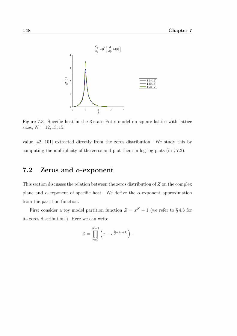
148 Chapter 7

Figure 7.3: Specific heat in the 3-state Potts model on square lattice with latticesizes, N = 12, 13, 15.

value [42, 101] extracted directly from the zeros distribution. We study this by

computing the multiplicity of the zeros and plot them in log-log plots (in § 7.3).

7.2 Zeros and α-exponent

This section discusses the relation between the zeros distribution of Z on the complex

plane and α-exponent of specific heat. We derive the α-exponent approximation

from the partition function.

First consider a toy model partition function Z = xN + 1 (we refer to § 4.3 for

its zeros distribution ). Here we can write

Z =N−1∏r=0

(x− e

iπN

(2r+1)).

Chapter 7 149

At limit N →∞, we have the free energy given by

limN→∞

f = limN→∞

1

NlnZ

= limN→∞

1

Nln

N−1∏r=0

(x− e

iπN

(2r+1))

= limN→∞

1

N

N−1∑r=0

ln(x− e

iπN

(2r+1)).

By Taylor expansion for x = eβ and small β, we have

limN→∞

f ∼ limN→∞

1

N

N−1∑r=0

ln

(1 + β −

(1 +

iπ

N(1 + 2r)

))

= limN→∞

1

N

N−12∑

r=−N−12

ln

(β +

πi

N(2r +N)

).

As N → ∞ the zeros are distributed uniformly with a fixed density. We could

write the free energy with the zeros distribution line density denoted a(y) as

limN→∞

f ∼ 1

2π

∫ ∞−∞

a(y) ln(β + iy) dy

where a(y) = 1.

Suppose we replace this constant density with other density which varying as we

move in the complex plot. We have the internal energy

U = − dfdβ

∼ − 1

2π

∫ ∞−∞

a(y)

β + iydy

=i

2π

∫ ∞−∞

a(y)

y − iβdy (7.4)

that has pole at y = iβ and a(y) = a(−y). This distribution give a first order phase

transition [58].

Alternatively, suppose the line density a(y) has power law relation [58], for small

y, that is

a(y) ∼ |y|1−p (0 ≤ p < 1). (7.5)

150 Chapter 7

This gives a continuous internal energy function and a divergence in specific heat at

p = 0. This corresponds to a second order phase transition.

By examining the asymptotic behaviour of U(β) as β → 0 [58], we may obtain

specific heat critical exponent for 0 < p < 1. The specific heat is given by

dU

dβ

β→0∼ β−p.

This relation gives the specific heat critical exponent α = p.

Suppose we consider a model that, like the two-dimensional Ising model, has a

line distribution of partition function zeros (for example as a function of eβ) in the

complex neighbourhood of the critical point.

Our hypothesis is that for sufficiently large lattices the distribution of zeros of

the partition function determines the α exponent. Specifically the hypothesis is that

the exponent is determined by fitting the ‘line density’ to a power law dependence

on distance from the critical point.

We can model this with a uniform positional distribution that has varying zeros

multiplicity. We could also vary the line separation between zeros. But for a finite

lattice approximation of continuum density, these two suggestion are similar [55].

Consider the zeros complex plane. We denote an equal range of imaginary part

of the zeros as y. Let a(y) be the multiplicity of zeros for each y. The partition

function can now be written in this form; for a suitable n ∈ N (with respect to the

zeros distribution),

Z =n∏y=1

(β + i

y

n

)a(y)

(7.6)

where y is arranged in increasing distance from critical point. The partition function

has zeros that are less dense near the critical point to more denser zeros as we move

out in the complex plane. Let N be the size of the system. This gives the free

Chapter 7 151

energy

f =1

NlnZ =

1

Nln

n∏y=1

(β + i

y

n

)a(y)

=1

N

n∑y=1

a(y) ln(β + iy). (7.7)

Taking the logarithm on both sides of relation (7.5), we have

log a(y) ∼ (1− p) log |y| (7.8)

which gives a gradient (1− p) in the log-log scale plane.

The idea of zeros multiplicity in function (7.6) will be used in analysing our zeros

data near the real axis in complex plane zeros distribution. We use relation (7.8)

to approximate the value of specific heat critical exponent α. We discuss this by

notion of line density of zeros distribution in the next section.

7.3 Analysis on zeros density distribution

In this section, we analyse the line density of the zeros distribution. The line density

is measured by the number of zeros in a subset of points in the complex zeros

distribution plane. The α-exponent is determined by fitting a straight line into the

log-log graph. This will gives the gradient m = 1− p and α = p.

For the finite lattice, we know that the finite size effects (explained in Chapter

4) are present in the zeros distribution. This also affect the log-log analysis. For

sufficiently large enough size, we expect the gradient of the log-log graph will become

stable hence converge to the result in thermodynamic limit.

If this is true, then the problem of finding the critical exponent of a specific

heat can be reduced to a problem of finding the log-log gradient. We may be able

to determine the log-log gradient by increasing the lattice sizes. Hence we can

determine the critical exponent. This simplification will assist the calculation of

this α-exponent.

152 Chapter 7

Three cases have been considered using this log-log analysis. They are briefly

listed as follows:

1. The 2-state Potts model and Ising model on square lattice - finite cases from

Onsager’s solution.

2. The 3-state Potts model on square lattice.

3. The accumulated case of the 3-state Potts model on square lattice.

The accumulated case above will be explained further in § 7.3.3.

0

0.2

0.4

0.6

0.8

1

1.2

1.4

0 0.5 1 1.5 2 2.5 3

Figure 7.4: Example: first quadrant with bin of equal size for square lattice Isingmodel, N = 50.

Consider the complex plane for zeros distribution. We call each space with equal

size a bin. See Figure 7.4. First, the first quadrant of complex plane is divided into

several bins of equal angle. Then the total number of zeros in each bin over distance

from the real axis is plotted in the log-log plot. The gradient of the logarithmic plot

is determined to represent the power law relation for comparison with the known

result.

Let b ∈ N be the number of total bins with equal angle from origin i.e. θ =π

2b.

And let ai be the number of zeros in each bin where i = 1, 2, · · · , b. The number of

zeros is counted only for those in the ferromagnetic region.

Chapter 7 153

The linear regression line fitting is used to fit the line of the zeros data. Due

to the quantisation effect in the finite case, the linear fitting is done only on the

angle near the transition point (first few bins). The y-axis is the logarithmic scale

for the number of zeros ai and the x-axis is the logarithmic scale for distance from

real axis in the complex plane. The distance is represented by a simple numbering

with x = 1, 2, ..., b.

Let m denotes the gradient of the linear fit. For comparison, we manually fit the

line on the log-log graph.

7.3.1 The 2-state Potts model and Ising model − finite case

from Onsager’s solution

Here we describe the analysis on 2-state Potts model on square lattices of sizes 19

by 19 and 20 by 20. We also analyse the Onsager’s Ising model zeros distribution

with lattice sizes 49 by 49, 50 by 50, 99 by 99 and 100 by 100.

Table 7.1: Approximated slope m of log-log plane for 19 × 19′ and 20 × 20′ squarelattices. The manual column is our own estimate directly on the log-log graph.

Lattice size 19× 19′ 20× 20′

Bin, b Lin. reg. Std. dev. Manual Lin. reg. Std. dev. Manual6 0.93899 0.16400 1.00 0.91110 0.21020 0.907 0.72474 0.12319 0.80 0.97427 0.12869 1.008 1.09710 0.22530 1.00 1.13670 0.27250 0.909 0.87645 0.10518 0.95 1.02096 0.11154 1.0010 0.95920 0.07519 1.00 1.07383 0.10632 0.9011 1.000e+00 2.415e-16 1.00

See Table 7.1. This table describes the approximation for gradient m of the

log-log plot for square lattice 19 by 19 and 20 by 20 of 2-state Potts model. The

standard deviation of the linear regression analysis is also shown in this table. The

column with total number of bins b is the variable for testing. As we vary the value

of b, we check the gradient and its standard deviation.

For 19 by 19 lattice size, it can be seen in Table 7.1 that the approximation

154 Chapter 7

reaches low standard deviation when we take the number of bins, b = 10. This

approximation suggests that the approximated value of α-exponent is nearly zero

i.e. α19 = 1− 0.95920 = 0.0408.

For comparison, we further test the zeros data for 20 by 20 lattice case. This

size improvement shows that the lowest standard deviation started to emerge when

number of bins is at b = 11. This approximation gives the approximated value of

α-exponent to be zero (1-1=0). Figures 7.5 and 7.6 present the linear regression line

fitting for the 19 by 19 and 20 by 20 case with increasing number of total bins.

1 2 5 10 20

12

510

20

x

y

(a) Number of bins, b = 6.

1 2 5 10 20

12

510

20

x

y

(b) Number of bins, b = 7.

1 2 5 10 20

12

510

20

x

y

(c) Number of bins, b = 8.

1 2 5 10 20

12

510

20

x

y

(d) Number of bins, b = 9.

1 2 5 10 20

12

510

20

x

y

(e) Number of bins, b = 10.

Figure 7.5: Lattice 19× 19 : Linear regression analysis on log-log graphs.

From the known result [101], this observation is very promising since we know

that α = 0 for the Ising model. For a large lattice size, the log-log gradient analysis

is a very convincing approach in finding the critical exponent of specific heat.

We examine the zeros from Onsager’s partition function on 49×49, 50×50, 99×99

and 100 × 100 square lattices. Tables 7.2 and 7.3 describe the approximation of

log-log linear fitting gradient by linear regression analysis and also by our own

estimation.

Chapter 7 155


Lattice size 49× 49′ 50× 50′

Bin, b Lin. reg. Std. dev. Manual Lin. reg. Std. dev. Manual6 0.70680 0.17581 0.80 0.68589 0.17008 0.857 0.96394 0.12327 0.95 0.74285 0.13096 0.908 0.88348 0.07914 0.90 0.89385 0.09973 1.009 0.94430 0.05673 1.05 0.85755 0.06194 0.9010 1.02143 0.15312 1.00 1.05898 0.12823 1.1511 0.90537 0.08267 1.25 0.97027 0.06215 1.0012 0.96817 0.08687 1.10 0.89355 0.06381 1.0013 0.88986 0.07570 1.10 0.97750 0.04518 1.1014 0.96536 0.07308 1.00 1.05585 0.05983 1.0015 0.99628 0.09292 1.00 0.98123 0.08653 1.0016 0.97097 0.07456 0.95 1.04545 0.06624 1.0517 1.04496 0.07042 0.95 0.96997 0.09009 1.1018 1.01593 0.07278 1.10 0.95723 0.07614 0.9519 1.03028 0.07994 1.00 0.97725 0.06966 1.0020 0.95314 0.08499 0.90 0.94095 0.06692 1.0021 1.01374 0.07093 1.00 0.98264 0.08228 1.0022 0.97289 0.04845 0.95 0.93796 0.06808 1.0023 1.00671 0.07221 0.95 1.05704 0.07892 1.2024 1.02687 0.06218 1.05 1.13146 0.06805 1.0025 0.96594 0.04661 1.00 1.01301 0.05130 1.0026 0.95291 0.05226 1.00 1.01507 0.03550 0.9527 0.97771 0.05102 0.95 0.93749 0.04586 1.1028 0.97275 0.04557 1.00 1.00687 0.03802 1/0029 0.97189 0.04521 1.00 0.95440 0.05054 1.0530 1.00256 0.08744 1.05 0.95792 0.06627 1.05

156 Chapter 7

Table 7.3: Approximated slope m of log-log plane for 99× 99′ and 100× 100′ squarelattices. The manual column is our own estimate directly on the log-log graph.

Lattice size 99× 99′ 100× 100′

Bin, b Lin. reg. Std. dev. Manual Lin. reg. Std. dev. Manual6 0.98823 0.09576 1.15 0.98618 0.10626 0.907 0.92509 0.07922 1.15 1.08718 0.06377 1.058 0.88728 0.08189 1.05 1.01864 0.05231 1.059 1.00604 0.07324 1.05 1.07185 0.06142 0.9510 0.95626 0.07023 1.00 1.11431 0.05931 1.0511 1.04726 0.06063 1.00 1.08076 0.04094 1.0012 0.98669 0.04702 1.10 1.04617 0.03913 1.0013 0.97308 0.05435 1.10 1.08313 0.05358 1.0514 0.95910 0.04875 1.00 1.05595 0.02985 1.1015 1.00735 0.05186 1.00 1.04609 0.05617 1.0016 0.96391 0.04085 0.90 1.02435 0.04026 1.1017 0.95895 0.04149 0.95 1.02347 0.03518 1.1018 0.97073 0.03453 1.05 1.01396 0.02934 0.9519 0.97381 0.03949 1.00 1.01797 0.03956 0.9520 1.00459 0.06219 1.05 1.07274 0.03707 1.0521 0.98633 0.04489 1.00 1.07150 0.04394 1.0022 0.99341 0.03493 1.10 1.05187 0.02727 1.0523 0.93009 0.03275 1.00 1.03297 0.01873 1.0524 0.96870 0.02774 1.05 0.99994 0.02763 0.9525 1.06193 0.03289 1.05 1.01458 0.03217 1.1026 0.94521 0.03168 1.00 1.01586 0.02909 0.9027 0.92396 0.03373 1.05 0.99821 0.02324 1.1028 0.96805 0.03442 1.00 1.02952 0.02803 1.0029 0.98326 0.03249 1.00 1.03293 0.03717 1.0030 0.96172 0.04282 0.95 1.04274 0.03229 1.00

Chapter 7 157

1 2 5 10 20

12

510

20

x

y


1 2 5 10 20

12

510

20

x

y


1 2 5 10 20

12

510

20

x

y


1 2 5 10 20

12

510

20

x

y


1 2 5 10 20

12

510

20

x

y


1 2 5 10 20

12

510

20

x

y

(f) Number of bins, b = 11.


Figures 7.7, 7.8, 7.9 and 7.10 show the linear regression line fitting for 49 ×

49, 50 × 50, 99 × 99 and 100 × 100 square lattices respectively. The approximation

gives many results with small deviation when we change the value of b. The gradients

are mostly very close to m ∼ 1 i.e. 0.9 < m < 1.1. For some bins, the quantisation

effect may dominate which are evident by the large standard deviation. For m ∼ 1,

this approximately gives the value of specific heat exponent α ∼ 1 − 1 = 0. This

analysis will converge to the known result − as shown in [101, p. 46].

For 100 by 100 square lattice, one can see that the log-log graph line fitting is

very close to the points. The change in the number of bins does not give a huge

effect on the distribution. The slope is approximately m ∼ 1 which gives α = 0.

158 Chapter 7

1 2 5 10 20 50 100 200

12

510

2050

100

200

x

y


1 2 5 10 20 50 100 200

12

510

2050

100

200

x

y


1 2 5 10 20 50 100 200

12

510

2050

100

200

x

y


1 2 5 10 20 50 100 200

12

510

2050

100

200

x

y


1 2 5 10 20 50 100 200

12

510

2050

100

200

x

y


1 2 5 10 20 50 100 200

12

510

2050

100

200

x

y


1 2 5 10 20 50 100 200

12

510

2050

100

200

x

y

(g) Number of bins, b = 16.

1 2 5 10 20 50 100 200

12

510

2050

100

200

x

y

(h) Number of bins, b = 17.

1 2 5 10 20 50 100 200

12

510

2050

100

200

x

y

(i) Number of bins, b = 18.

1 2 5 10 20 50 100 200

12

510

2050

100

200

x

y

(j) Number of bins, b = 19.

1 2 5 10 20 50 100 200

12

510

2050

100

200

x

y

(k) Number of bins, b = 20.


Chapter 7 159

1 2 5 10 20 50 100 200

12

510

2050

100

200

x

y


1 2 5 10 20 50 100 200

12

510

2050

100

200

x

y


1 2 5 10 20 50 100 200

12

510

2050

100

200

x

y


1 2 5 10 20 50 100 200

12

510

2050

100

200

x

y


1 2 5 10 20 50 100 200

12

510

2050

100

200

x

y


1 2 5 10 20 50 100 200

12

510

2050

100

200

x

y


1 2 5 10 20 50 100 200

12

510

2050

100

200

x

y


1 2 5 10 20 50 100 200

12

510

2050

100

200

x

y


1 2 5 10 20 50 100 200

12

510

2050

100

200

x

y


1 2 5 10 20 50 100 200

12

510

2050

100

200

x

y


1 2 5 10 20 50 100 200

12

510

2050

100

200

x

y



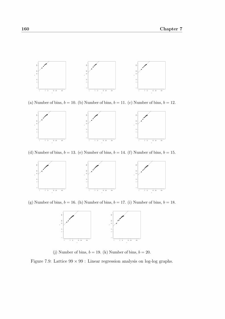
160 Chapter 7

1 5 10 50 100 500

15

1050

100

500

x

y


1 5 10 50 100 500

15

1050

100

500

x

y


1 5 10 50 100 500

15

1050

100

500

x

y


1 5 10 50 100 500

15

1050

100

500

x

y


1 5 10 50 100 500

15

1050

100

500

x

y


1 5 10 50 100 500

15

1050

100

500

x

y


1 5 10 50 100 500

15

1050

100

500

x

y


1 5 10 50 100 500

15

1050

100

500

x

y


1 5 10 50 100 500

15

1050

100

500

x

y


1 5 10 50 100 500

15

1050

100

500

x

y


1 5 10 50 100 500

15

1050

100

500

x

y



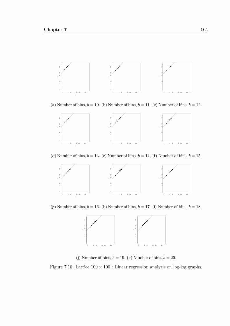
Chapter 7 161

1 5 10 50 100 500

15

1050

100

500

x

y


1 5 10 50 100 500

15

1050

100

500

x

y


1 5 10 50 100 500

15

1050

100

500

x

y


1 5 10 50 100 500

15

1050

100

500

x

y


1 5 10 50 100 500

15

1050

100

500

x

y


1 5 10 50 100 500

15

1050

100

500

x

y


1 5 10 50 100 500

15

1050

100

500

x

y


1 5 10 50 100 500

15

1050

100

500

x

y


1 5 10 50 100 500

15

1050

100

500

x

y


1 5 10 50 100 500

15

1050

100

500

x

y


1 5 10 50 100 500

15

1050

100

500

x

y



162 Chapter 7

7.3.2 The 3-state Potts model

Here we present the analysis on several largest cases for the 3-state Potts model

zeros distributions that we managed to produced in this thesis.

See Tables 7.4 and 7.5. The gradient m for individual case for 12 by 12, 13

by 13, 14 by 14 and 15 by 17 square lattices are presented in these tables with

the comparison between linear regression analysis and our manual estimation. As

before, the standard deviation of the linear regression analysis is also shown in these

tables.

The linear regression line fitting for 12 by 12 square lattice is shown in Figure

7.12. Based on the result in Table 7.4, one can see that the standard deviations are

mostly over 0.1. We suspect the number of zeros is not enough in the first quadrant

(see Figure 7.11a) to approximate the limiting slope through the log-log analysis.

The zeros are still too far from the real axis in the complex plane. The zeros in

antiferromagnetic region is not counted for the log-log graph.


Lattice size 12× 12′ 13× 13′

Bin, b Lin. reg. Std. dev. Manual Lin. reg. Std. dev. Manual6 0.59478 0.10304 0.70 0.54000 0.18192 0.807 0.90741 0.06768 0.90 0.74789 0.13769 0.558 0.59781 0.11707 0.60 0.76448 0.08011 0.609 0.69353 0.10397 0.75 0.77963 0.12546 0.6010 0.76040 0.11860 1.00 0.65835 0.05620 0.75


Lattice size 14× 14′ 15× 17′

Bin, b Lin. reg. Std. dev. Manual Lin. reg. Std. dev. Manual6 0.58580 0.16110 0.75 0.49330 0.11493 0.607 0.76880 0.09357 0.60 0.53440 0.13894 0.808 0.69276 0.11134 0.70 0.61090 0.08523 0.709 0.67331 0.08984 0.60 0.70270 0.08235 0.6010 0.74003 0.09145 0.70 0.71160 0.10301 1.0011 0.71280 0.04786 0.7012 0.70470 0.06792 0.70

Chapter 7 163

0

0.5

1

1.5

2

2.5

3

0 0.5 1 1.5 2 2.5 3

12x12’

(a)

0

0.5

1

1.5

2

2.5

3

0 0.5 1 1.5 2 2.5 3

13x13’

(b)

0

0.5

1

1.5

2

2.5

3

0 0.5 1 1.5 2 2.5 3

14x14’

(c)

0

0.5

1

1.5

2

2.5

3

0 0.5 1 1.5 2 2.5 3

15x17’

(d)

Figure 7.11: Zeros distribution at quadrant 1 for 3-state Potts model on squarelattice of a) 12 by 12, b) 13 by 13, c) 14 by 14 and d) 15 by 17.

1 2 5 10

12

510

x

y


1 2 5 10

12

510

x

y


1 2 5 10

12

510

x

y


1 2 5 10

12

510

x

y


1 2 5 10

12

510

x

y


Figure 7.12: Lattice 12x12 : Linear regression analysis on log-log graphs.

164 Chapter 7

1 2 5 10

12

510

x

y


1 2 5 10

12

510

x

y


1 2 5 10

12

510

x

y


1 2 5 10

12

510

x

y


1 2 5 10

12

510

x

y



Consider the 13 by 13 square lattice. The linear regression line fitting is shown in

Figure 7.13. Similar to 12 by 12 case, the standard deviation in Table 7.4 gives values

mostly more than 0.1. The number of zeros in the first quadrant (see also Figure

7.11b for 13 by 13 case) are not enough to suggest a good gradient approximation.

Next, Figures 7.14 and 7.15 present the linear regression line fitting for larger

cases with 14 by 14 and 15 by 17 lattice sizes respectively. More zeros are located

in the first quadrant of the complex-eβ plane for larger cases (see Figure 7.11).

As the total number of bins b changes we observe the emergence of the gradient

with small standard deviation, for example in the case with 15 by 17 lattice size.

The approximation converge to the known value from experiment (also the folklore

theory) for the α-exponent of 3-state Potts model i.e. α = 1/3 [98, 101].

In Table 7.5, the estimation for the case with total number of bins equal to 11 and

12 has estimated gradient value of 0.7128 and 0.7047 respectively. This estimations

is the closest approximation we have so far. This value gives α close to 1/3. The

bigger the lattice size, a better convergent sequence can be made from this analysis.

Chapter 7 165

1 2 5 10

12

510

x

y


1 2 5 10

12

510

x

y


1 2 5 10

12

510

x

y


1 2 5 10

12

510

x

y


1 2 5 10

12

510

x

y



1 2 5 10 20

12

510

20

x

y


1 2 5 10 20

12

510

20

x

y


1 2 5 10 20

12

510

20

x

y


1 2 5 10 20

12

510

20

x

y


1 2 5 10 20

12

510

20

x

y


1 2 5 10 20

12

510

20

x

y



166 Chapter 7

For some estimation however, the quantisation effect may dominate, for example

as shown in 15 by 17 case when the total number of bins b = 10. Our manual

estimation and the linear regression approximation do not coincide each other. The

reason for this is due to the data chosen for the linear regression line fitting. The

line is fitted on the data that may dominated by quantisation effect or finite size

effect (that includes points that are far from the critical point). In contrast, our

manual fitting give us more freedom in choosing the points from the bins that is

near to the critical point. The linear graph shown in 7.15d convinced us that the

estimation is affected by the finite size effect.

7.3.3 The accumulated case of 3-state Potts model

In this section we consider another type of zeros data collection for testing.

Table 7.6: Approximated slope m of log-log plane for accumulated zeros from 12×12′, 13 × 13′, 14 × 14′ and 15 × 17′ square lattices. The manual column is our ownestimate directly on the log-log graph.

Lattice size All zerosBin, b Lin. reg. Std. dev. Manual

6 0.54650 0.13678 0.757 0.76419 0.10170 0.658 0.66258 0.08293 0.809 0.70973 0.08226 0.8010 0.71434 0.08326 0.7511 0.72440 0.11357 0.7012 0.83374 0.11708 0.6513 0.79471 0.11728 1.2014 0.72016 0.05601 0.8015 0.67004 0.04927 0.7516 0.70098 0.05753 0.8017 0.73147 0.04802 0.8018 0.74239 0.03766 0.7019 0.66271 0.05214 0.7020 0.69746 0.06845 0.7521 0.65775 0.05629 0.8022 0.62372 0.06816 0.70

To add more varieties to the study, we consider a case with zeros taken from

several big lattice cases that we have investigated. The zeros are now taken from

Chapter 7 167

1 2 5 10 20 50

12

510

2050

x

y


1 2 5 10 20 50

12

510

2050

x

y


1 2 5 10 20 50

12

510

2050

x

y


1 2 5 10 20 50

12

510

2050

x

y


1 2 5 10 20 50

12

510

2050

x

y


1 2 5 10 20

12

510

20

x

y


1 2 5 10 20

12

510

20

x

y


1 2 5 10 20

12

510

20

x

y


1 2 5 10 20

12

510

20

x

y


1 2 5 10 20

12

510

20

x

y


1 2 5 10 20

12

510

20

x

y


1 2 5 10 20

12

510

20

x

y

(l) Number of bins, b = 17.

Figure 7.16: Lattice 12 × 12′ to 15 × 17′ : Linear regression analysis on log-loggraphs.

168 Chapter 7

1 2 5 10 20

12

510

20

x

y


1 2 5 10 20

12

510

20

x

y


1 2 5 10 20

12

510

20

x

y


1 2 5 10 20

12

510

20

x

y


1 2 5 10 20

12

510

20

x

y


Figure 7.17: Lattice 12×12′ to 15×17′ : Linear regression analysis on log-log graphs(cont.).

all these lattices i.e. 12 by 12, 13 by 13, 14 by 14 and 15 by 17. We call them the

accumulated zeros data.

As before, the number of zeros in each bin is computed and plotted in the

log-log plot. Again, we vary the number of total bins b. For this case, we let

b = 1, 2, . . . , 22.

See Table 7.6 for the approximated value of the linear regression and our manual

estimation. Figures 7.16 and 7.17 show the log-log plot and their linear regression

line fitting.

Since a lot of zeros are now involved, we can investigate and vary the total number

of bins b into larger values as compared to the individual case in the previous section

§ 7.3.2. Table 7.6 shows several results of estimation from linear regression analysis

with small standard deviation less than 0.1. In the last five estimation from b = 19

and above, we have several nice estimations with small deviation. These estimations

are very close to the known α-exponent value of 1/3.

Chapter 7 169

This result suggests that the analysis produces a good approximation if we have

many zeros data. The higher number of bins means smaller range of distance (or

small angle θ) in the imaginary axis of the complex plane zeros distribution. The

estimation particularly involves the zeros that is very close to the critical point xc.

The analysis is done on the 3-state Potts model case and the Ising model because

we can directly compare our estimation with the result from [101]. The promising

results from this analysis can be extended to zeros distributions for other models and

lattices. This is an open problem since more experimental result and bigger lattice

result are needed for checking and comparison. In the next chapter, we continue

with an analysis for a model with multiple phases.

Chapter 8

Analytical machinery for multiple

phases in ZQ-symmetric model

In this chapter we investigate the energy and entropy relation [27] relative to phase

transitions in terms of our exact solutions.

We discuss the possibility of multiple transitions between fully ordered and

disordered states. Next we study the polynomial term of the partition function

Z and plot the accumulated value of the terms towards Z = 0 at complex coupling

values that are roots of Z close to the transition points. The final section contains

graphs of the specific heat. This analysis is focused on the 2- and 3-state Potts

models and the Z5- and Z6-symmetric models.

8.1 Candidates for 3 phase models

The solved case of Ising model [75, 92] for example showed the existence of single

phase transition at x = 1 +√

2 in the ferromagnetic (ferro) [44] region.

On the other hand, the study of ZQ-symmetric model partition function showed

the possibility of multiple phase transitions for some energy function χ [58]. Recall

the result in Chapter 6. For specific χ, as defined in § 6.1, we can see in Figure 8.1,

a pattern of zeros distribution with single arc for example when χ = (3, 1, 0) and

171

172 Chapter 8

double arc for example when χ = (3, 2, 0) which move close to the positive real axis

as the lattice size increases (see also § 6.2).

-2

-1

0

1

2

-2 -1 0 1 2

8x8’

(a)

-2

-1

0

1

2

-2 -1 0 1 2

8x8’

(b)

Figure 8.1: The 8 by 8 zeros distribution for a) χ = (3, 1, 0) and b) χ = (3, 2, 0).

8.2 Energy vs entropy

We describe the idea of energy and entropy competition in a model partition function

in this section. First we describe the idea of energy-entropy in a model of phase

transition. Then we describe a modification aiming to explain two transitions.

To support the existence of two transitions, a new kind of transition mechanism

as compared to order/disorder transition is needed for explanation. The claim is

that there are two stages of disordered state in the system. From first stage to the

second stage, this change corresponds to the second phase transition − for example

from a fairly disordered to a completely random disordered state.

8.2.1 Single order/disorder phase transition

Recall the expectation value (1.4) of an observable quantity O of physical system

given by

〈O〉 =∑σ∈Ω

p(σ)O(σ) (8.1)

Chapter 8 173

where p(σ) =e−βH

Z.

We shall observe the energy-entropy competition as we vary the temperature T

[52, 58]. Recall that β = 1/(kBT ).

At low T (high β), e−βH → 0 as β → ∞. The system preferred to be in the

ordered state. The dominant contribution is coming from the high magnitude of H

despite the low entropy. At low T the energy dominate the system.

In contrast, at high T (low β), e−βH → 1 as β → 0. The system is not dominated

by H but by the number of configurations that give the entropy of the system.

The configuration with relatively little order among the spins may be regarded as

representative of the system. At high T the entropy dominate the system.

At low T where the system is in ordered state, there is a strong interaction

between all the particles and its neighbours. At high T , the system is in disordered

state where the spin variables prefer to point at different directions.

Peierls [78] shows a rigorous arguments to support the emergence of phase

transition between order (low energy in the Potts model) and disorder (high

entropy). Peierls in his paper describes the phase transition by the emergence of

line separations in the dual picture of configurations as in § 6.3.1.

8.2.2 Two phase transitions

For the system with two phase transitions we can describe the transition mechanism

by the idea of two different stages of entropy appearance. The idea of the second

phase transition can also be described through the behaviour of the line separation

(see § 6.3.1).

The increase in temperature will drive the line separations to become longer (see

Figure 8.2) or change the distance among the vortices. This system will have extra

entropy from this long string lines which then balance out the energy penalty due

to the different spin orientation. This energy and entropy competition drives the

second phase transition. At large enough temperature, the fairly disordered state

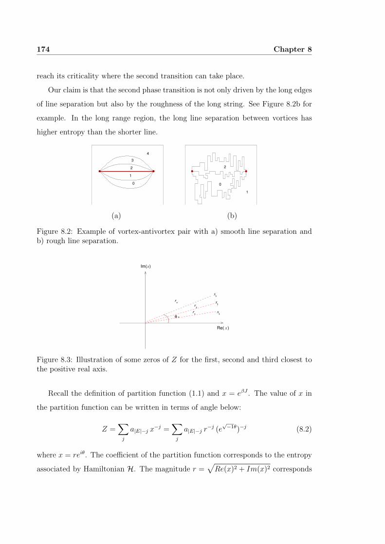
174 Chapter 8

reach its criticality where the second transition can take place.

Our claim is that the second phase transition is not only driven by the long edges

of line separation but also by the roughness of the long string. See Figure 8.2b for

example. In the long range region, the long line separation between vortices has

higher entropy than the shorter line.

1

0

22

0

4

1

3

(a) (b)

Figure 8.2: Example of vortex-antivortex pair with a) smooth line separation andb) rough line separation.

θ

Im( )x

Re( )x

x

x1

2

3x

r

r

2

1

3

r3

Figure 8.3: Illustration of some zeros of Z for the first, second and third closest tothe positive real axis.

Recall the definition of partition function (1.1) and x = eβJ . The value of x in

the partition function can be written in terms of angle below:

Z =∑j

a|E|−j x−j =

∑j

a|E|−j r−j (e

√−1θ)−j (8.2)

where x = reiθ. The coefficient of the partition function corresponds to the entropy

associated by Hamiltonian H. The magnitude r =√Re(x)2 + Im(x)2 corresponds

Chapter 8 175

to the magnitude of complex zeros of the partition function. The angle θ is

measure from the real positive axis. These three components are the main factors

contributing to the energy-entropy competition in this system.

The concept of two different stages in the disordered phase may be extended

to more disordered stages as we increase the value of temperature. These

different stages mean other energy-entropy battle in the microscopic detail of

the configuration state. The configuration state is transformed to more random

disordered state where the vortex-antivortex pair may become very close to each

other and the configuration states are at random.

8.3 ZQ-symmetric model partition function

We describe the line separation in a configuration state and further relate them to

the energy-entropy competition in a partition function. Recall Ω as the set of all

configuration states and σ ∈ Ω. We consider the Z5- and Z6-symmetric models on

square lattice in this section.

The configuration state σ can be illustrated by the local spin boundaries between

two different spin configurations drawn on the dual lattice. For a state σ that has

one variable in different orientation from the rest of the spin variables, the total

energy is reduced by 4 corresponding to 4 dual edges (see Figure 8.4a).

Similarly, if there are two neighbouring spin variables with the same orientation

but different from the orientation of the others, the total energy is reduced by 6

(see Figure 8.4b). The partition function can be written with exponent given by the

value of energy penalty. The energy penalty is drawn as the edges of line separation

in the dual lattice.

In this thesis, we are always interested to study the behaviour of configuration

states near the phase transition. We analyse the partition function polynomial

relative to its zero value. The accumulated summations of the polynomial terms are

plotted for specific value of the root x.

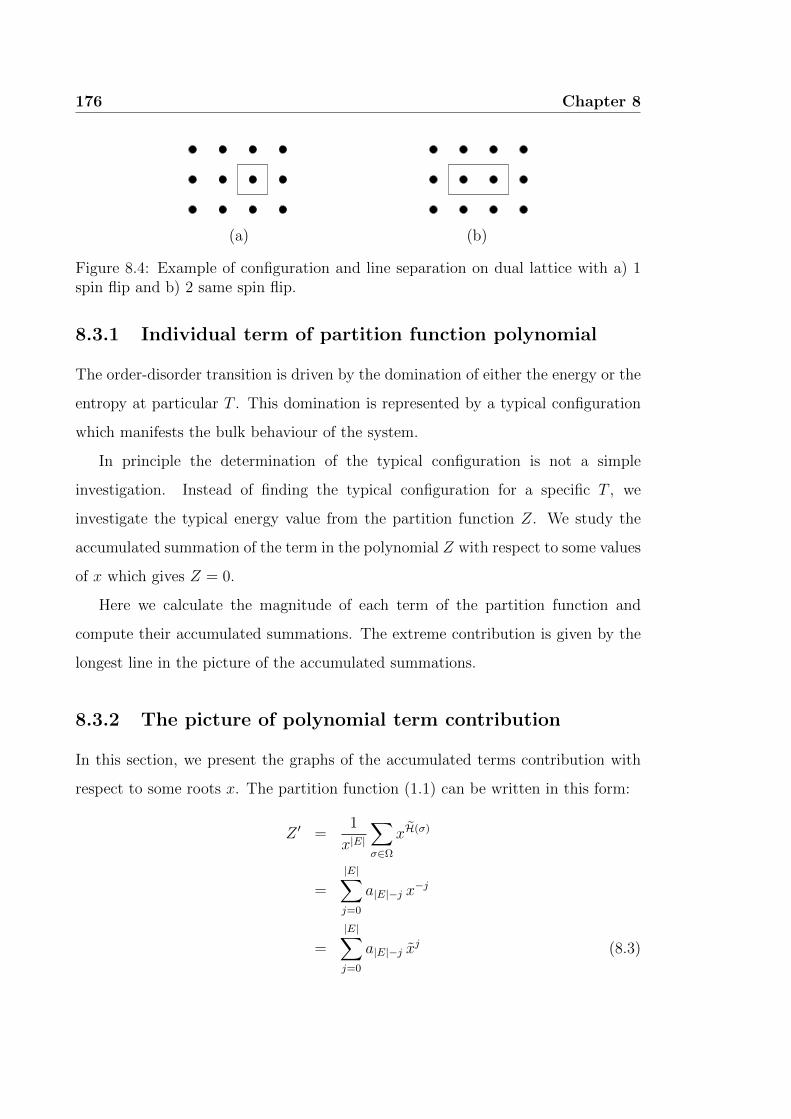
176 Chapter 8

(a) (b)

Figure 8.4: Example of configuration and line separation on dual lattice with a) 1spin flip and b) 2 same spin flip.

8.3.1 Individual term of partition function polynomial

The order-disorder transition is driven by the domination of either the energy or the

entropy at particular T . This domination is represented by a typical configuration

which manifests the bulk behaviour of the system.

In principle the determination of the typical configuration is not a simple

investigation. Instead of finding the typical configuration for a specific T , we

investigate the typical energy value from the partition function Z. We study the

accumulated summation of the term in the polynomial Z with respect to some values

of x which gives Z = 0.

Here we calculate the magnitude of each term of the partition function and

compute their accumulated summations. The extreme contribution is given by the

longest line in the picture of the accumulated summations.

8.3.2 The picture of polynomial term contribution

In this section, we present the graphs of the accumulated terms contribution with

respect to some roots x. The partition function (1.1) can be written in this form:

Z ′ =1

x|E|

∑σ∈Ω

xH(σ)

=

|E|∑j=0

a|E|−j x−j

=

|E|∑j=0

a|E|−j xj (8.3)

Chapter 8 177

where aj is the coefficient of the polynomial, x = 1/x and H is as in (1.2). The

above partition function (8.3) is written based on the energy penalty given by the

length of line separation in the dual lattice.

We compute the accumulated summations of the partition function as below.

Let Zj = a|E|−j xj and p0 = Z0. We have

p1 = p0 + Z1

p2 = p1 + Z2

p3 = p2 + Z3

...

p|E| = p|E|−1 + Z|E|.

The difference between two accumulated summations |pj+1 − pj| is the net

contribution of each new term j + 1. The length of the line from pi to pi+1 is

the total contribution given by the term Zi+1. Here we study the step by step terms

cancellation of the partition function by plotting each value of pj. The root x of Z

is chosen close to critical point in the positive real axis.

Recall that for T ∼ 0, the Boltzmann weight x = e−βJ is close to 0. This value

shows the energy domination. The system is in an ordered state. In contrast, for

T → ∞, all the Boltzmann weight has weight equal to 1. The entropy represented

by the coefficient of the partition function polynomial is dominating the system.

The middle term of the polynomial with the highest entropy is the most probable

state.

At low T when x = 0, only the constant term in the polynomial survives. This

term represents the ordered state when all spin variables spin in the same direction.

We may explain the partition function by this condition. Let n,m ∈ N. The

first n terms of the polynomial are representing the ordered state i.e. ferromagnetic

(ferro) state [41, 44, 45]. And the final m terms correspond to another kind of

ordered state i.e. antiferromagnetic (antiferro) state. The middle part is the most

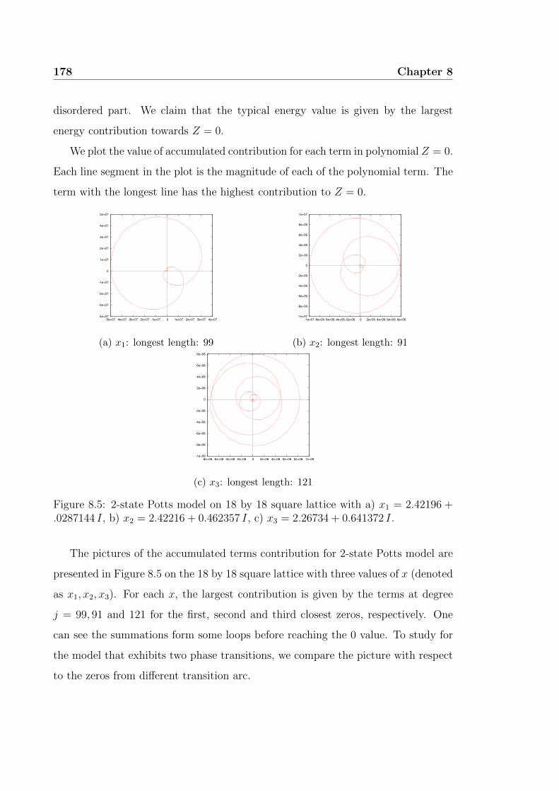
178 Chapter 8

disordered part. We claim that the typical energy value is given by the largest

energy contribution towards Z = 0.

We plot the value of accumulated contribution for each term in polynomial Z = 0.

Each line segment in the plot is the magnitude of each of the polynomial term. The

term with the longest line has the highest contribution to Z = 0.

-4e+07

-3e+07

-2e+07

-1e+07

0

1e+07

2e+07

3e+07

4e+07

5e+07

-5e+07 -4e+07 -3e+07 -2e+07 -1e+07 0 1e+07 2e+07 3e+07 4e+07

(a) x1: longest length: 99

-1e+07

-8e+06

-6e+06

-4e+06

-2e+06

0

2e+06

4e+06

6e+06

8e+06

1e+07

-1e+07 -8e+06 -6e+06 -4e+06 -2e+06 0 2e+06 4e+06 6e+06 8e+06

(b) x2: longest length: 91

-1e+09

-8e+08

-6e+08

-4e+08

-2e+08

0

2e+08

4e+08

6e+08

8e+08

-8e+08 -6e+08 -4e+08 -2e+08 0 2e+08 4e+08 6e+08 8e+08 1e+09

(c) x3: longest length: 121

Figure 8.5: 2-state Potts model on 18 by 18 square lattice with a) x1 = 2.42196 +.0287144 I, b) x2 = 2.42216 + 0.462357 I, c) x3 = 2.26734 + 0.641372 I.

The pictures of the accumulated terms contribution for 2-state Potts model are

presented in Figure 8.5 on the 18 by 18 square lattice with three values of x (denoted

as x1, x2, x3). For each x, the largest contribution is given by the terms at degree

j = 99, 91 and 121 for the first, second and third closest zeros, respectively. One

can see the summations form some loops before reaching the 0 value. To study for

the model that exhibits two phase transitions, we compare the picture with respect

to the zeros from different transition arc.

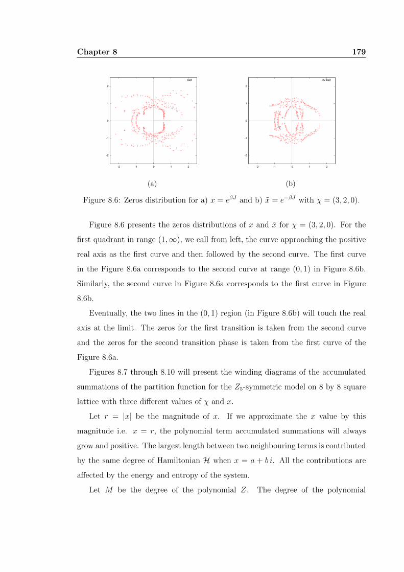
Chapter 8 179

-2

-1

0

1

2

-2 -1 0 1 2

8x8’

(a)

-2

-1

0

1

2

-2 -1 0 1 2

inv-8x8’

(b)

Figure 8.6: Zeros distribution for a) x = eβJ and b) x = e−βJ with χ = (3, 2, 0).

Figure 8.6 presents the zeros distributions of x and x for χ = (3, 2, 0). For the

first quadrant in range (1,∞), we call from left, the curve approaching the positive

real axis as the first curve and then followed by the second curve. The first curve

in the Figure 8.6a corresponds to the second curve at range (0, 1) in Figure 8.6b.

Similarly, the second curve in Figure 8.6a corresponds to the first curve in Figure

8.6b.

Eventually, the two lines in the (0, 1) region (in Figure 8.6b) will touch the real

axis at the limit. The zeros for the first transition is taken from the second curve

and the zeros for the second transition phase is taken from the first curve of the

Figure 8.6a.

Figures 8.7 through 8.10 will present the winding diagrams of the accumulated

summations of the partition function for the Z5-symmetric model on 8 by 8 square

lattice with three different values of χ and x.

Let r = |x| be the magnitude of x. If we approximate the x value by this

magnitude i.e. x = r, the polynomial term accumulated summations will always

grow and positive. The largest length between two neighbouring terms is contributed

by the same degree of Hamiltonian H when x = a + b i. All the contributions are

affected by the energy and entropy of the system.

Let M be the degree of the polynomial Z. The degree of the polynomial

180 Chapter 8

-3e+06

-2e+06

-1e+06

0

1e+06

2e+06

3e+06

-2e+06 -1e+06 0 1e+06 2e+06 3e+06 4e+06


-2000

-1500

-1000

-500

0

500

1000

1500

-2000 -1500 -1000 -500 0 500 1000 1500 2000


-800000

-600000

-400000

-200000

0

200000

400000

600000

800000

-600000 -400000 -200000 0 200000 400000 600000 800000

(c) x3 : longest length: 60

Figure 8.7: Z5-symmetric model on 8 by 8 square lattice with χ = (2, 1, 0): a) x1 =2.10969+0.479109 I, b) x2 = 2.42248+0.665705 I and c) x3 = 2.07525+0.734082 I.

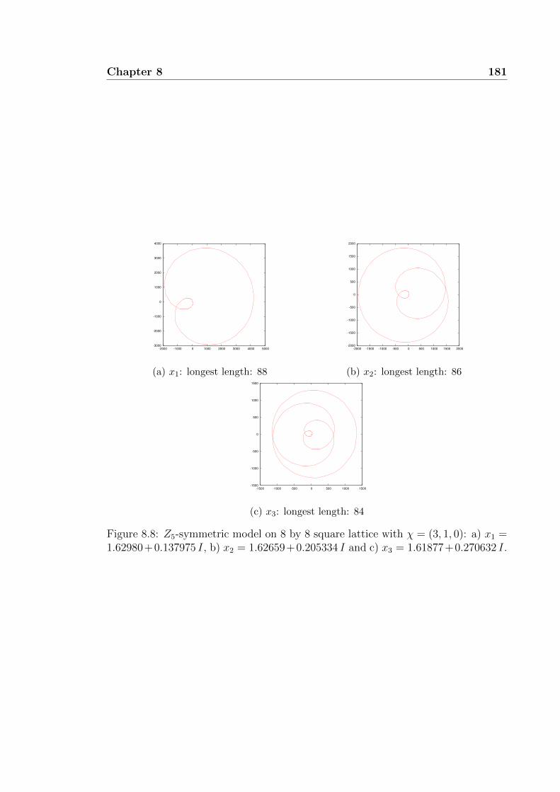
Chapter 8 181

-3000

-2000

-1000

0

1000

2000

3000

4000

-2000 -1000 0 1000 2000 3000 4000 5000


-2000

-1500

-1000

-500

0

500

1000

1500

2000

-2000 -1500 -1000 -500 0 500 1000 1500 2000


-1500

-1000

-500

0

500

1000

1500

-1500 -1000 -500 0 500 1000 1500


Figure 8.8: Z5-symmetric model on 8 by 8 square lattice with χ = (3, 1, 0): a) x1 =1.62980+0.137975 I, b) x2 = 1.62659+0.205334 I and c) x3 = 1.61877+0.270632 I.

182 Chapter 8

-4e+92

-3e+92

-2e+92

-1e+92

0

1e+92

2e+92

3e+92

4e+92

-4e+92 -3e+92 -2e+92 -1e+92 0 1e+92 2e+92 3e+92


-8e+11

-6e+11

-4e+11

-2e+11

0

2e+11

4e+11

6e+11

8e+11

1e+12

-8e+11 -6e+11 -4e+11 -2e+11 0 2e+11 4e+11 6e+11 8e+11 1e+12


-8e+16

-6e+16

-4e+16

-2e+16

0

2e+16

4e+16

6e+16

8e+16

-8e+16 -6e+16 -4e+16 -2e+16 0 2e+16 4e+16 6e+16 8e+16


Figure 8.9: First curve: Z5-symmetric model on 8 by 8 square lattice with χ =(3, 2, 0): a) x1 = 1.64360 + 0.334788 I, b) x2 = 1.58838 + 0.476209 I and c) x3 =1.37846 + 0.546351 I.

-800

-600

-400

-200

0

200

400

600

800

-600 -400 -200 0 200 400 600 800


-300

-200

-100

0

100

200

300

400

-400 -300 -200 -100 0 100 200 300


Figure 8.10: Second curve: Z5-symmetric model on 8 by 8 square lattice with χ =(3, 2, 0): a) x = 2.36582 + 0.771200 I and b) x = 2.24748 + 0.114699 I.

Chapter 8 183

partition function for the 8 by 8 square lattice with χ = (3, 2, 0) is equal to 360.

In general, let a square lattice have Ny row and Nx column vertices with open

horizontal and periodic vertical boundary conditions. Take the energy list denoted

as χ = (χ1, χ2, ..). Then the degree of the polynomial is given by

M = χ1(2NxNy −Ny).

For any mi < M ∈ N, let (0,m1) be the first range consists of m1+1 terms. Next,

the (m1 +1,m2) be the second range consists of m2−m1 terms. Then (m2 +1,M/2)

be the third and so on. This categorisation can be illustrated as below:

mm2

m1

0 MM/2m = m3 4 5

Figure 8.11: Polynomial range categorisation for x.

The first term with zero degree is in the ferromagnetic state where all spin

variables point in the same direction. No energy penalty gives zero degree in the

polynomial. The second part is where the energy penalty increases. The energy

penalty is represented by the non-zero degree of the polynomial. The middle part

of the polynomial is the range where the system is in a random and completely

disordered state. This part has the highest number of entropy. The final part is

again the ordered part of antiferromagnetic state. Each spin variable prefers to point

in different direction from its neighbours.

For χ = (2, 1, 0) and χ = (3, 1, 0), their zeros distributions suggest the existence

of a single phase transition. The largest contributions for the terms cancellation

towards zero value are described in the Figures 8.7 and 8.8. The largest contribution

for both cases have small degree exponent.

We claim that the term that gives the largest contribution marks the occurrence

of a phase transition. With the high number of spin directions for Q = 5, the system

can be in total disordered state even with small energy penalty. The observations

for both cases of χ = (2, 1, 0) and χ = (3, 1, 0) are similar to the 2-state Potts model

which also exhibit only one phase transition.

184 Chapter 8

The χ = (3, 2, 0) in addition is another example for the Z5-symmetric model.

For this case, there exist a possible multiple phase transitions shown by the double

curve in the ferro region of the zeros distribution. The largest contributions for 5

different zeros in this case fall into two different ranges of polynomial terms. Figures

8.9 and 8.10 show the diagrams for the zeros taken from the first and second curve

of zeros distribution with x = eβJ , respectively.

The largest contribution for the zeros in second curve falls in the early part

of the polynomial. The degree of the polynomial term is small suggesting a little

disorder for the zeros in the second curve. In contrast, the largest contribution for

the zeros in the first curve falls into the part that is closer to the middle part of

the polynomial. This behaviour suggests a different kind of disordered phase will

emerges.

-2

-1

0

1

2

-2 -1 0 1 2

inv-8x8’

(a)

-2

-1

0

1

2

-2 -1 0 1 2

inv-8x8’

(b)

Figure 8.12: Zeros distribution for x = e−βJ with a) χ = (3, 2, 0, 0) and b) χ =(3, 2, 1, 0).

The Figures 8.14 through 8.19 present the accumulated summations graphs for

the Z6-symmetric model. The case with χ = (2, 1, 0, 0) in Figure 8.14 is believed to

exhibit only one phase transition based on the comparison of its zeros distribution

and the graph of specific heat (shown in § 8.4).

See Figures 8.14a and 8.14b. In both cases, their typical energy fall

approximately in the same energy range. In contrast, Figure 8.14c shows different

Chapter 8 185

value for its large term contribution. Since we know that this case only has one

transition point, we know that this different is due to the finite effect on the zeros

value. The third zeros lies off the curve in the zeros distribution as compared to the

first and second zeros (see Figure 8.13).

-2

-1

0

1

2

-2 -1 0 1 2

8x8’

Figure 8.13: Zeros distribution for x = eβJ with χ = (2, 1, 0, 0).

The case with χ = (3, 1, 0, 0) in Figure 8.16 also shows the existence of one phase

transition based on its zeros distribution in complex plane. All the three largest term

contributions are approximately in the same degree range.

For χ = (3, 2, 0, 0), this case is another example which exhibits two phase

transitions. See Figure 8.15. The existence of two curves in the ferro region near

the positive real axis gives evidence of this claim (see Figure 8.12). The graph of

accumulated summations for the zeros in the first curve is shown in Figure 8.17 and

the second curve is shown in Figure 8.18 .

For χ = (3, 2, 1, 0) the first and second zeros fall into approximately the same

energy range. However for the third zeros the largest contribution is given by energy

penalty at term x32. This distribution may be either because of the finite size effect

on its zeros distribution or due to the existence of multiple transitions. To exactly

check this observation, a bigger lattice is needed for investigation, i.e. N > 8.

In the thermodynamic limit, we expect the largest terms contribution will be

given by a significant value as compared to the contributions from other terms

186 Chapter 8

-2.5e+07

-2e+07

-1.5e+07

-1e+07

-5e+06

0

5e+06

1e+07

1.5e+07

2e+07

2.5e+07

-1.5e+07-1e+07 -5e+06 0 5e+06 1e+07 1.5e+07 2e+07 2.5e+07 3e+07


-4e+06

-3e+06

-2e+06

-1e+06

0

1e+06

2e+06

3e+06

4e+06

-4e+06 -3e+06 -2e+06 -1e+06 0 1e+06 2e+06 3e+06 4e+06


-3000

-2500

-2000

-1500

-1000

-500

0

500

1000

1500

2000

-2500 -2000 -1500 -1000 -500 0 500 1000 1500 2000 2500


Figure 8.14: Z6-symmetric model on 8 by 8 square lattice with χ = (2, 1, 0, 0): a) x =2.08847 + 0.405804 I, b) x = 2.08267 + 0.622161 I and c) x = 2.42583 + 0.658524 I.

-2

-1

0

1

2

-2 -1 0 1 2

8x8’

Figure 8.15: Zeros distribution for x = eβJ with χ = (3, 2, 0, 0).

Chapter 8 187

-6000

-4000

-2000

0

2000

4000

6000

8000

-4000 -2000 0 2000 4000 6000 8000 10000


-4000

-3000

-2000

-1000

0

1000

2000

3000

-4000 -3000 -2000 -1000 0 1000 2000 3000


-2000

-1500

-1000

-500

0

500

1000

1500

2000

2500

-2000 -1500 -1000 -500 0 500 1000 1500 2000 2500



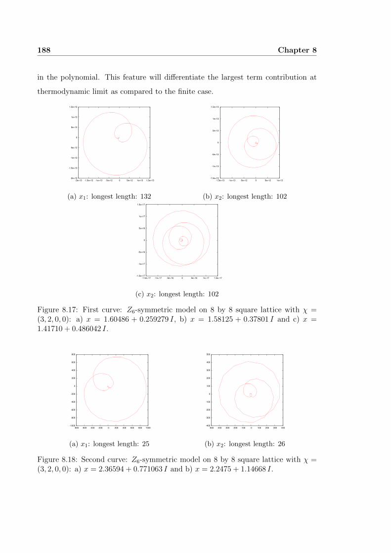
188 Chapter 8

in the polynomial. This feature will differentiate the largest term contribution at

thermodynamic limit as compared to the finite case.

-2e+13

-1.5e+13

-1e+13

-5e+12

0

5e+12

1e+13

1.5e+13

-2e+13 -1.5e+13 -1e+13 -5e+12 0 5e+12 1e+13 1.5e+13


-1.5e+13

-1e+13

-5e+12

0

5e+12

1e+13

1.5e+13

-1.5e+13 -1e+13 -5e+12 0 5e+12 1e+13


-1.5e+17

-1e+17

-5e+16

0

5e+16

1e+17

1.5e+17

-1.5e+17 -1e+17 -5e+16 0 5e+16 1e+17 1.5e+17


Figure 8.17: First curve: Z6-symmetric model on 8 by 8 square lattice with χ =(3, 2, 0, 0): a) x = 1.60486 + 0.259279 I, b) x = 1.58125 + 0.37801 I and c) x =1.41710 + 0.486042 I.

-1000

-800

-600

-400

-200

0

200

400

600

800

-800 -600 -400 -200 0 200 400 600 800 1000


-400

-300

-200

-100

0

100

200

300

400

500

-500 -400 -300 -200 -100 0 100 200 300 400


Figure 8.18: Second curve: Z6-symmetric model on 8 by 8 square lattice with χ =(3, 2, 0, 0): a) x = 2.36594 + 0.771063 I and b) x = 2.2475 + 1.14668 I.

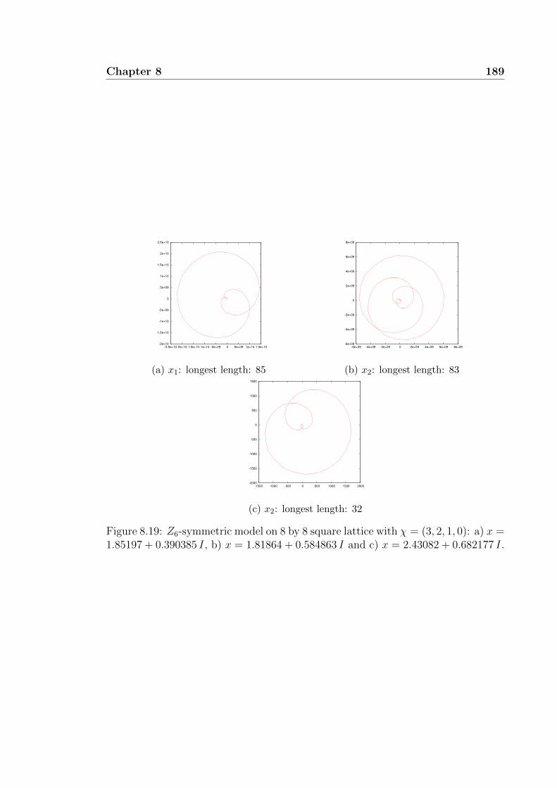
Chapter 8 189

-2e+10

-1.5e+10

-1e+10

-5e+09

0

5e+09

1e+10

1.5e+10

2e+10

2.5e+10

-2.5e+10-2e+10-1.5e+10-1e+10 -5e+09 0 5e+09 1e+10 1.5e+10


-6e+09

-4e+09

-2e+09

0

2e+09

4e+09

6e+09

8e+09

-6e+09 -4e+09 -2e+09 0 2e+09 4e+09 6e+09 8e+09


-2000

-1500

-1000

-500

0

500

1000

1500

-1500 -1000 -500 0 500 1000 1500 2000



190 Chapter 8

8.4 Graph comparison of specific heat

In this section we present a list of graphs for specific heat formula that are generated

from the partition function.

At constant volume V , a specific heat is defined by the amount of heat Q required

to increase a temperature T , i.e. CV =

(∂Q

∂T

)V

. In statistical mechanics, the

specific heat equation can be generated from the partition function (see § 1.3). The

specific heat is given byCVkB

= −β2 d2 lnZ

dβ2.

A sudden peak in the graph of specific heat over β is the signal of phase transition

[7, 35]. A discontinuous peak at thermodynamic limit is due to the discontinuity of

the second derivative of free energy.

We present the specific heat graphs for the 2- and 3-state Potts models and also

the Z5- and Z6-symmetric models for some energy list χ.

8.4.1 2- and 3-state Potts models’ specific heat

Figure 8.20 shows the graph of specific heat for the 2-state Potts model on the square

lattice with size N = 16, 18 and 20. From this plot, as the size increases the peak

of the graph also increases and the graph become steeper.

Similarly, Figure 8.21 shows the specific heat graph for the 3-state Potts model

on the square lattice of size N = 12, 13 and 15. Here the sharp peak in the graph

increases as the size increases. This behaviour in the middle of the graph is similar

to the 2-state Potts model. However the peak shown here is given by a smaller

lattice size as compared to the 2-state case. At infinite size, the peak is expected

to be discontinuous at βc that is at the critical temperature Tc of phase transition.

The single peak is in accordance with the prediction of the single transition through

the existence of a particular single curve in the graph of zeros distribution in the

complex plane. The specific heat graph support this single transition claim.

Chapter 8 191

Figure 8.20: Specific heat plot forCVkB

vs β with N = 16, 18, 20.

Figure 8.21: Specific heat plot forCVkB

vs β with N = 12, 13, 15.

192 Chapter 8

8.4.2 Z5- and Z6-symmetric models’ specific heat

Here we continue with the specific heat graph for the ZQ-symmetric model with

Q = 5 and 6 for some value of χ.

(a)

(b)

Figure 8.22: Z5-symmetric model: Specific heat graph for a) 8× 8 with different χand b) 7× 9, 8× 8, 9× 9 for χ = (3, 2, 0).

Figure 8.22 shows the specific heat graph for Z5-symmetric model with three

Chapter 8 193

(a)

(b)

Figure 8.23: Z6-symmetric model: Specific heat graph on square lattice a) 8 × 8with different χ and b) 6× 7, 7× 7, 8× 8 for χ = (3, 2, 0, 0).

194 Chapter 8

energy list χ = (2, 1, 0), (3, 1, 0) and (3, 2, 0). We can see the different peak behaviour

among these three χ values. For the χ = (2, 1, 0) and χ = (3, 1, 0), the single peak

suggests a single phase transition whereas for the χ = (3, 2, 0) the two peaks suggest

two phase transitions. Figure 8.22b presents the graph for χ = (3, 2, 0) for three

increasing lattice size N = 7, 8, 9.

We further consider the case of Z6-symmetric model. Figure 8.23 presents the

graph of specific heat with χ = (2, 1, 0, 0), (3, 1, 0, 0), (3, 2, 0, 0), (3, 2, 1, 0). The

specific heat curves for χ = (2, 1, 0, 0) and χ = (3, 1, 0, 0) each has only single

peak that corresponds to single transition.

The graph for χ = (3, 2, 1, 0) however has a peak which is not entirely sharp. As

shown in the zeros distribution, it has a possibility of either single or double curve

move closer to the positive real axis. A bigger lattice is needed to describe this case

correctly.

The graph for χ = (3, 2, 0, 0) in contrary shows obvious multiple peaks. These

two peaks are the evidence for two phase transitions. This observation is in

accordance with the multiple curves in the positive real axis of its zeros distribution.

We plot for this case with different lattice size as in Figure 8.23b. The bigger the

size, the sharper the peak will be.

8.5 Discussion

The study of polynomial terms of partition function is aimed to find the largest term

contribution of this function. This term is believed to have the most domination

over the cancellation of magnitude in its partition function. The largest contribution

will suggests a typical energy penalty that exists near the transition point.

As expected, the first kind of transition is just between the ordered and

disordered phases. The largest contribution is represented in the region just after

the fully ordered state represented by the constant term of the polynomial. Then we

can see that the zeros in the second curve has the largest contribution somewhere

Chapter 8 195

between the first disordered state and the middle part of the polynomial. Here the

energy penalty is high given by many edges in the dual lattice. This observation

suggests a different kind of disordered phase will starts to emerge soon afterwards.

We illustrate these phases in Figure 8.24.

1ordered

disordered

1st

1

disordered

2 nd

Figure 8.24: Ordered-disordered states illustration (not scaled).

The distinction between these two kind of disordered phases will be more obvious

at large lattice and certainly at the thermodynamic limit. The graph of specific heat

meanwhile shows the existence of phase transition through the peak in the graph.

The study of the polynomial term contribution support the determination of the

multiple phase transitions. The study provides one more detail about the system

i.e. the typical energy represented by the largest term contribution for Z = 0.

For the second phase transition however, it is not enough to determine the

existence only based on the change in the details of configuration state. The Peierls’

argument must be implemented again to support the existence of the second phase

transition.

This problem is still open − no equivalent to Peierls’ argument that prove the

existence of two transitions. The possibility is evidence in the zeros distribution

especially for Z5- and Z6-symmetric model. This observation is supported by the

behaviour in the graph of specific heat.

Conclusion

We have studied the partition functions and their zeros for Ising, Q-state Potts and

ZQ-symmetric models on several crystal lattices. The zeros are plotted in complex

Argand plane to study the analytic structure of the zeros distributions. Our research

supports the claim that this structure suggests the behaviour of physical observables

at thermodynamic limit related to phase transition.

The study of zeros distribution give the approximation of the physical critical

exponent value. We can also simultaneously study the analytic structure at

ferromagnetic and antiferromagnetic phases.

We may be able to exactly predict the locus of zeros if we can reach large enough

lattice size. For the moment, although it is very interesting to further extend the

zeros distribution to larger cases, the computing resources in hand is limiting our

study. The implementation of parallel computing is one option for improvement.

197

Appendices

A Algorithm for zeros finding

The Newton-Raphson (NR) method is a numerical algorithms for finding roots ofpolynomial equation. The complex roots of partition function when Z = 0 are foundusing this method.

Let n ≥ 0 and let the number of iterations xn be the estimated zeros at iterationn and f be the polynomial function. Then the NR method is performed by thefollowing iterative formula;

xn = xn−1 −f(xn−1)

f ′(xn−1). (A.1)

Theorem A.1. Given a positive integer n ≥ 1 and any choice of coefficientsa0, a1, ..., an ∈ C, such that an 6= 0, define the function f : C→ C by setting

f(z) = anzn + ...+ a1z + a0, ∀z ∈ C.

In other words, f is a polynomial function of degree n. Then1. given any complex number w ∈ C, we have that f(w) = 0 if and only if there

exists a polynomial function g : C→ C of degree n− 1 such that

f(z) = (z − w)g(z), ∀z ∈ C.

2. there are at most n distinct complex numbers w for which f(w) = 0. In otherwords, f has at most n distinct roots.

3. (Fundamental Theorem of Algebra, restated) there exist exactly n+ 1 complexnumbers w0, w1, ..., wn ∈ C (not necessarily distinct) such that

f(z) = w0(z − w1)(z − w2)...(z − wn),∀z ∈ C.

In other words, every polynomial function with coefficients over C can be factoredinto linear factors over C.

For numerical computation, let TOL be the predetermined tolerance (orestimated error) and x0 be the initial value. The NR method calculate the

199

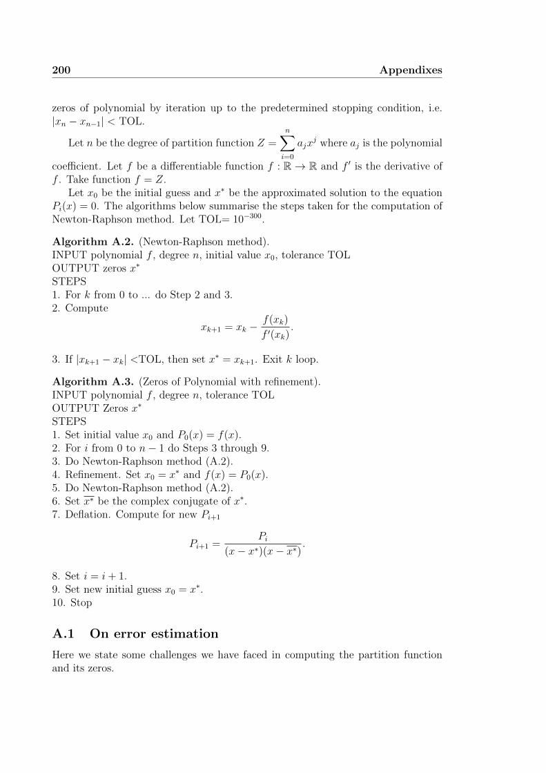
200 Appendixes

zeros of polynomial by iteration up to the predetermined stopping condition, i.e.|xn − xn−1| < TOL.

Let n be the degree of partition function Z =n∑i=0

ajxj where aj is the polynomial

coefficient. Let f be a differentiable function f : R → R and f ′ is the derivative off . Take function f = Z.

Let x0 be the initial guess and x∗ be the approximated solution to the equationPi(x) = 0. The algorithms below summarise the steps taken for the computation ofNewton-Raphson method. Let TOL= 10−300.

Algorithm A.2. (Newton-Raphson method).INPUT polynomial f , degree n, initial value x0, tolerance TOLOUTPUT zeros x∗

STEPS1. For k from 0 to ... do Step 2 and 3.2. Compute

xk+1 = xk −f(xk)

f ′(xk).

3. If |xk+1 − xk| <TOL, then set x∗ = xk+1. Exit k loop.

Algorithm A.3. (Zeros of Polynomial with refinement).INPUT polynomial f , degree n, tolerance TOLOUTPUT Zeros x∗

STEPS1. Set initial value x0 and P0(x) = f(x).2. For i from 0 to n− 1 do Steps 3 through 9.3. Do Newton-Raphson method (A.2).4. Refinement. Set x0 = x∗ and f(x) = P0(x).5. Do Newton-Raphson method (A.2).6. Set x∗ be the complex conjugate of x∗.7. Deflation. Compute for new Pi+1

Pi+1 =Pi

(x− x∗)(x− x∗).

8. Set i = i+ 1.9. Set new initial guess x0 = x∗.10. Stop

A.1 On error estimation

Here we state some challenges we have faced in computing the partition functionand its zeros.

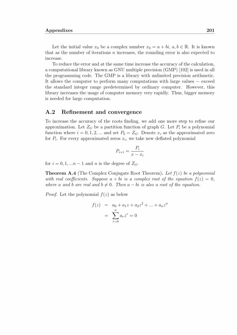
Appendixes 201

Let the initial value x0 be a complex number x0 = a + bi, a, b ∈ R. It is knownthat as the number of iterations n increases, the rounding error is also expected toincrease.

To reduce the error and at the same time increase the accuracy of the calculation,a computational library known as GNU multiple precision (GMP) [102] is used in allthe programming code. The GMP is a library with unlimited precision arithmetic.It allows the computer to perform many computations with large values − exceedthe standard integer range predetermined by ordinary computer. However, thislibrary increases the usage of computer memory very rapidly. Thus, bigger memoryis needed for large computation.

A.2 Refinement and convergence

To increase the accuracy of the roots finding, we add one more step to refine ourapproximation. Let ZG be a partition function of graph G. Let Pi be a polynomialfunction where i = 0, 1, 2, ... and set P0 = ZG. Denote xi as the approximated zerofor Pi. For every approximated zeros xi, we take new deflated polynomial

Pi+1 =Pi

x− xi

for i = 0, 1, ...n− 1 and n is the degree of ZG.

Theorem A.4 (The Complex Conjugate Root Theorem). Let f(z) be a polynomialwith real coefficients. Suppose a + bi is a complex root of the equation f(z) = 0,where a and b are real and b 6= 0. Then a− bi is also a root of the equation.

Proof. Let the polynomial f(z) as below

f(z) = a0 + a1z + a2z2 + ...+ anz

n

=n∑r=0

arzr = 0

202 Appendixes

where all ar are real. Then

f(z) =n∑r=0

ar(z)r = 0

n∑r=0

ar(z)r = 0

n∑r=0

ar(z)r = 0

n∑r=0

ar(z)r = 0

f(z) = 0.

Therefore, the zeros appear to be in conjugate pair.

By the complex conjugate root theorem A.4, for any polynomial with complexzero, its complex conjugate is also a zero of the polynomial. For each Pi, the NRmethod is implemented to find the remaining zeros.

For refinement, the NR method is implemented on the original ZG. At each Piwhen i > 0, we take the approximated zero x′i as the initial value for NR methodon ZG. The new root from this step is accepted as the new approximated zero xi ofZG. This step is repeated each time we find the root for the polynomial Pi.

At some condition, we may have a convergence problem when there exist two ormore zeros located very close together or when there exist zeros with multiplicitygreater than 1. The existence of real zeros may also contribute to the problem. Thusit is worth to check the possible real zeros from the beginning of the computation.

For the case where two or more zeros are close together, we can choose differentinitial value after some number of iterations where it can redirect the program tocompute the zeros finding. A lot of checking need to be done in order to detect this.

Appendixes 203

B Onsager’s solution

We present the Onsager’s solution using rotational matrix approach as discussed byKaufman in [40].

Note that the horizontal and vertical nearest neighbour interaction for the squarelattice can be represented by rotational matrix

MR(θ) =

(cos(θ) sin(θ)− sin(θ) cos(θ)

)where the det(MR(θ)) = 1, so the complex eigenvalues are exp(±iθ).

Denote W as the rotational matrix and Wab(θ) be the matrix rotation in ab-plane.For any i and 2N dimensions of rotational matrix, let

wii+1(θ) = 1i−1 ⊕MR(θ)⊕ 12N−i−1.

The idea is to replace the product of V1 =

(N∏i=1

ti

)and V2 =

(N∏i=1

ti(i+1)

)(from

(4.2)) by a matrix rotation W = W1W2. The W1 and W2 are rotational matricesgiven by

W1 =N∏i=1

w2i 2i−1(2iθ)

and

W2 =N∏i=1

w2i+1 2i(2iθ′).

Let c = cos(2iθ), c′ = cos(2iθ′), s = sin(2iθ) and s′ = sin(2iθ′). For example, ifN = 4,

W1 = w12w34w56w78 =

c s−s c

c s−s c

c s−s c

c s−s c

204 Appendixes

W2 =

c −sc s−s c

c s−s c

c s−s c

s c

.

Then

W = W1W2 =2N∏i

waibi(θi) (B.2)

where all ai, bi are distinct. Let z = e2πikN so zN = 1. Since the dimension of a

rotational matrix is smaller than the dimension of transfer matrix T , the problemof finding the eigenvalue for partition function is reduced to only for finding theeigenvalue of the corresponding rotational matrix.

Using Fourier transform, we define vector

fz =

1z2

z4

z6

...z2N−2

where vz = fz ⊗

(10

)and v′z = fz ⊗

(01

).

Then

W1

(vzv′z

)=

(c −ss c

)(vzv′z

),

W2

(vzv′z

)=

(c′ −zs′

−z−1s′ c′

)(vzv′z

)and

W

(vzv′z

)=

(cc′ + ss′z−1 cs′z − sc′−cs′z−1 + sc′ ss′z + cc′

)(vzv′z

)(B.3)

where we denote image of W as W (z) =

(cc′ + ss′z−1 cs′z − sc′−cs′z−1 + sc′ ss′z + cc′

). Since the

det(W (z)) = 1, we write the eigenvalues as λ± = e±lz .For example, suppose we have an Ising model on N by M square lattice. From

Martin [58] and Valani [92], the transfer matrix have the largest magnitude of

Appendixes 205

eigenvalue given by λ0

λ0 = exp

(1

2

N∑k=1

le2iπk/N

). (B.4)

Denote λ = λ0. The eigenvalues of rotational matrix are elz and e−lz . Thenby the relation between the transfer matrix and the rotational matrix, the sum ofeigenvalues is equal to the trace of W (z) [84, p. 249]

elz + e−lz = 2

(cos(2iθ) cos(2iθ′) +

z + z−1

2sin(2iθ) sin(2iθ′)

).

For large M , the partition function

ZNM ∼ λM . (B.5)

Using identities cosh(x) ≡ ex + e−x

2, cosh(x) ≡ cos(ix) and sinh(x) ≡ i sin(ix), we

have

cosh(lz) = cosh(2θ) cosh(2θ′)− z + z−1

2sinh(2θ) sinh(2θ′) (B.6)

where lz is the solution for the eigenvalue (B.4). Using identities sinh(2θ′) =sinh(2θ)−1 and coth(2θ′) = cosh(2θ) in isotropic case θ = θ′ gives

lz = cosh−1

(coth(2θ′) cosh(2θ′)− z + z−1

2

).

Again, using identity for simplification that is

cosh−1 x = ln(x) +1

π

∫ π

0

ln(1 + x cos y) dy

=1

π

∫ π

0

dy ln(2x− 2 cos y),

this gives

lz =1

π

∫ π

0

ln

(2(

coth(2θ′) cosh(2θ′)− z + z−1

2

)− 2 cos y

)dy

le2iπk/N =1

π

∫ π

0

ln (2 coth(2θ′) cosh(2θ′)− 2 cos(2πk/N)− 2 cos y) dy.

Substitute this into Equation (B.4), we get

lnλ =1

2

N∑k=1

1

π

∫ π

0

dy ln(2 coth(2θ′) cosh(2θ′)− 2 cos(2πk/N)− 2 cos y

). (B.7)

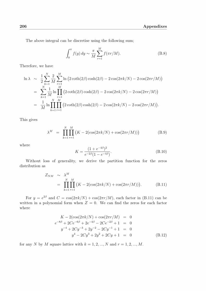
206 Appendixes

The above integral can be discretise using the following sum;∫ π

0

f(y) dy ∼ π

M

M∑r=1

f(πr/M). (B.8)

Therefore, we have

lnλ ∼ 1

2

N∑k=1

2

M

M∑r=1

ln(2 coth(2β) cosh(2β)− 2 cos(2πk/N)− 2 cos(2πr/M)

)=

N∑k=1

1

Mln

M∏r=1

(2 coth(2β) cosh(2β)− 2 cos(2πk/N)− 2 cos(2πr/M)

)=

1

Mln

N∏k=1

M∏r=1

(2 coth(2β) cosh(2β)− 2 cos(2πk/N)− 2 cos(2πr/M)

).

This gives

λM =N∏k=1

M∏r=1


)(B.9)

where

K =(1 + e−4β)2

e−2β(1− e−4β). (B.10)

Without loss of generality, we derive the partition function for the zerosdistribution as

ZNM ∼ λM

=N∏k=1

M∏r=1


). (B.11)

For y = e2β and C = cos(2πk/N) + cos(2πr/M), each factor in (B.11) can bewritten in a polynomial form when Z = 0. We can find the zeros for each factorwhere

K − 2(cos(2πk/N) + cos(2πr/M) = 0

e−8β + 2Ce−6β + 2e−4β − 2Ce−2β + 1 = 0

y−4 + 2Cy−3 + 2y−2 − 2Cy−1 + 1 = 0

y4 − 2Cy3 + 2y2 + 2Cy + 1 = 0 (B.12)

for any N by M square lattice with k = 1, 2, ..., N and r = 1, 2, ...,M .

App

endix

es

207

C Coefficient of partition function

Here we present one example of partition function coefficient. The coefficient of 3-state Potts model on 15 by 17 squarelattice is given below:

Degree Coefficient

0 29274766481378105714861373681423215500710370344961 2506290942057917100360939516702911612675637215232002 112126344456763294560865233519942129088271652697478403 3481849894622622192679714855629910189630274418104793604 84154854497325899311301185214447906819142468711847483205 1683947700206119377954945419229979604807572528272820785606 28988883005484127765212601896745484045042964584420094892807 440652281732844699161016974433118496768778743468093225368808 6026378653307089929676700678107580681539281080409255073078809 752001188539346822900478604206194724132455627257437421472916010 8655984585475022752081914396984065573314355125111351142778693611 92707621390173110004645260493019513235893427604124490760330066012 930405357114647524963220163762282229013893059939635988325111908013 8800572996820980642335157661331367959626984626455750550103397688014 78839899398199705884328993537307838805905040036682566467019200480015 671692353955152504420418722956426511334506916650468089098057704534016 5461606149431429110909392128051825681068190033835523452886258029621017 42513303751017484746898409445485691788058175386789319175082343068555018 317645474950622237090029556950115564609383895563921473813501351990918019 2283451637124050973619341588695467554033493388771521713222189963670665020 15826047411828725701495370048579031271361822575561217046707402069856151221 105946196861200730875361675102384181113924976828743941650864074715819231022 686193777226028343193223855631177286663708805381839946550934054904187732023 4306262569637582648472510238085891238280630685016050855987635389323782662024 26219716685372581278370458604782217804705089584051162634106326665974112823025 155080272750476602457566152333521020999153140554199192506595741100828237774226 892003037499538306852662008173183658182086822677207402853782377300874692608027 4994547288598574703421120748670484882962603139541722214255242314619181853615028 27248861013090935583148446838832056501184865348484895797033227500597616132300029 144975038349721333424502804616451194501937068599782609960573751749643336485775030 752787525805068531510424794407741941184198798531395247614332453519999892878642031 3817702414769916004313633874413946914333593784095523086268724514006088614662807032 18922372574692767584554396518239836817134789582719285875807721505069575851002881033 91720387143059504798785104919336510559396765683262625450667177721889966324516465034 435038226818790293209904087431182791087721270166896233710357762157190828573629043035 2020217025907775115432580096938360329428793837418269737562777345617741640507355949836 9189680423958532651794982978988135020150143559100644859029278711280500657162894591037 40967884755918957172038712791250505037372263934919725015661568869338399559848275682038 179070430390957516417285900298021334494756332718383411105252524116654162397102072921039 767761665326707357077822722498948099816641998194308784297066838276827395924836519876040 3230172340405590973986213340831390041116594272200752163863110427014925289130206070515041 13340943983514874502228063814238523057713284953566944813637935260391782564478194524971042 54108440419426968554105877852533571169776556745720110846162325888967356982811663772124043 215580192685857986406676496931586283854250882803121392158977203499588121181796144051550044 844030787429453752152079082413650374518308496062485883958796688862370606779712485638852045 3248227892643145347042773993803285193658988870522726105266451528769641232815219879605833446 12291364744416775172663061245626624592497802929415153297774361590109459679737876609795912047 45744585125691638029571634874997324641944501746857524708253087736869768092454060735368123048 167486627148527343280527880920561908182704781755816639327520323148679162649497058283337193049 6034357296321008999534931967917909598290795096564203853869628192792527661154657090844953380

208

Ap

pendix

es

50 2139917193722436675465041037382573714167588059838762351333653228500287106003017701747185042851 7470986409025615916406062695611944049242498363917943261932465697245044290716233091835392101052 25684407721625886531244975762008152150514705020865390401208107118100117674771274667061190914053 86968761541624606368007391210288554548973024494597481775343005721063443527986131281884291267054 290099350649970450748056950499275432299379803201129174608669056947644682803053046047924775075055 953463203670742858471610914983263946894124033194934072622539184201102827309781457145887723654056 3088270606671079903576809685430016622051409938156132822012641306237867449163997298353407589572057 9859576209859814731056687900788304316563509362491352401416734536426231068767995288812923656354058 31031788739090477920813834209729322442921269616812671251686655028154308439462681071559454950554059 96301328412776516360436791647568947087030361019495713699961949458059324603914616341947739699179060 294715596271936677527588746893651796440964755117575544907246372430549158076439842759063944634997061 889580309963040702646850061196450847863984719309155068875133042876869919924862246378632655899491062 2648754597170057414998201755129378357026761969512808356812194102939748131621232335925371833457014063 7780969874843034410549701238113275171014884453526053705988157142455025420033757898459927951507429064 22553806271397520065576690550235159714282987770309330550695606079911765310659247237939404247194653065 64514381930553783275624329759281164748936648007421394104417144138269427679194641508887177271234133666 182137021311353106521966502496772677389267734355397420296914008708532596447499026427010937479295368067 507571634097770936809605128154422361494863101087005264870786252102431487706337690005370408944991410068 1396382574961306251455682895848249397008750294253094945205366225838635991430049891318201695916153996069 3792872042518504445135477387626450350376671252107798429544039359675890946544490746608741865968867820070 10172686305969671945775586889317992894276427648291596154479150870264476620359956075073940835735761374671 26943384015060272537756119827087274927076936072975122750299557765838016188692146135529567262720854529072 70479271110756918525582898328139900986030427475239282888564830481308141095376278371121949914455351513073 182098204073988622572261066569567680192271377634772185066215640500675292968347744010243519164086328633074 464756715990823745164801713880787429017678220450330420469492259859295884605210438271895228835814764605075 1171819689430509616399144118751651494236644291585610953055289525037939615149710735941076675866351363371476 2919100280101266356077675149270022466806813900887313521874093824093089454974901999732476555374226909406077 7185004590740211590340553232680297505843132200605507674599369524062702053633964170736813039307542893755078 17475529939830672374331204364925459919919681650116120660961292491263377114424193232216234827768598832037079 42004245292802841077530287994179251451307243733443877885072633084890627379094014028112508930101843317429080 99781182901839159538138004585612071209986967660169862442955562128311297362661536165794722845856041624762481 234276503598022860856165784071406374337229090217467641005859231443316644756405514601062176578879770430294082 543706301381319514942785669970705862135220681696084778271811223590278842528780505818940573003468908541097083 1247341692378000179067809134618539170215271749939039055831258874253190303740828512285791079737261013417531084 2828921213967627535027511154410235880318954345355926341897999984960980401547389339140650217393751910349456085 6343056093993763967123957485419415992501737671019037484204758481933975572102711238743360273785275465112368886 14061950386801694738200459508829201976576384738613573158304925903853750110077291184433247480717043936606543087 30823930434861739084107746754492718797780961941318849461612485307569195932389921232645577615771299930771609088 66811495814604494222131350901374076390448040103734708839385726609231532389994752872553809163837203172378822089 143205452226689477025951947736033376894502151040014839964836630319784093431097875935197821478798941427219734090 303554550742060446249181415510915913405856652604318352230149573445323321174594642325058527396570314323204106491 636364099079556146258752984189436681720847352684063100247408089335369606896846621575922606593202592292303625092 1319436432965497638645542125158187782946966272593061072237834750851980692812623525834421344049757592549502289093 2705867890241341986513842334266392380705367861604736046615292803707995738672235967257270144437141423479423782094 5488842530981348728546169837574978348504155078162296764803820572107310869287504684524184672353466912717795960095 11013645802113284983387522624689213068565235636554430962473150427926444019459196612043653665221213992562069939496 21861353043188653929704699404480372130909628102981895756090221320819506075617901261969684869689693763085112793097 42927678136243765115222806028221431325602348924930814382739173154829614911202460258897339899745367243914051770098 83393159119598530468370181148671537081597197175263043469530415914462059549969108626229602949481784221261359556099 1602779518357281517644370369990085907121579694569669447945861892940911973689421094444322451999636315017307410880100 3047786819402257389983650622351040239180213954525086771325068571159618889767223231254527046136026769536224297758101 5734286893420872952954739812244310018083019953402330705459454121769672037521806974563086421311044431778319671660102 10675158942498189393086450675516376797486001156724474981162392676628217285307922396414902612368044076494781416520103 19664593192122962548446772223938028062439183512054543700375240489745814910789030080863685609228937724752495771400104 35844817804528021619052080525679106545001888003298363408983385179139679715839935853532959138369360403556803132470105 64656655966574723443483664644282007849620853086307766488941033911578162663461801341692850686703261596444377109970106 115414340328397574386338295916875100822432663276013229306056400549307567781057717295542550888015610958123810512400107 203882421926633523432737190270500856682614359493761590275116138493343617150332475107922409396234648750012144409040108 356440195269863271632637843207580801485389849008189017792078315302327392952935082355134101720691668218406091836350109 616727706328139223548455042584219976422243512110576701617349264635813676002906109852765333174446780750789297131140

App

endix

es

209

110 1056118852094698226680216855195661253533324717382595406241654230745879582793231075264981432065226550946311062227438111 1790016276140849753296209510846435737754707186600624512123872891666409133988665132436808069604979900946648950584910112 3002880011360252889405570024428136550500163409561869106538108140643350691053850328040941321082130959622543892685580113 4986174087890595888703047977722043793805695412543360772326985122648297995579613393688554490859312550535312204319630114 8195146005170721743000351378750844763591907317946596741559388076380076439395878678616603448205981273694507542624240115 13332659981508790672585143660588484246942648271360194976416578325284226061125537428022183108613535225356008875691758116 21471309774967067511880617454920293532971996576337599475583743338985868423258599976312923839285444395819693549628160117 34228858256547945983824166177506862703965387226086225402513648079680050780813584008148027562172786313623280642680520118 54016780800836843330558203971664238924189815773266128923906294166663193622715673450649491250196349322837453253740870119 84387365784355812507363499013998201052002094978625371224515002394941026393039499742724671700718983755505167331670700120 130511393590192888384193830618432090294627436925623098688217782120433766976072952475171941255730794228307128552168444121 199825681089605332506017570204955739679963768381078854169670886050385790702389034079317673186587424937658238872455620122 302897351915583727186950577280282544955128998231604639492532157587334092161911679258409773327871337254399913655305880123 454558930252508350483956194888257834050265035950239297864470870869684744577980958967631806405970226394331810238806610124 675374304618852007492199366157965415105230319363434425240836888750564813871072994073052928720077185989919150907585230125 993498965735122005033366585041552292942880774030691449354503100652014965929356168128351494694700801722724273767738126126 1446997024088975895351351384234584583676568673884587019202139888107500170197675793305303404408472547827546282579473700127 2086670362456572310930302512678901514790756473284117744989889850916448816905857864360261095733253913413230106761090770128 2979439643212847546108273416519622149422962524036119543888953953143683268690346587504433504163011003565664019024618710129 4212290470142958229151712777926927028446459308950907237228050323618808242725149403627355930906644989084412171485067320130 5896758693140582121263517929206588196154727346021344439745924822932071576876949602066954887084553415443966241487697368131 8173875078067151648615569567423430148955625726557063431051807033773665317366388459582312682449601014416271012863859710132 11219420750812840328932789801362066880049752286916955934521413154164020751948924817617977969312868957899716067449511010133 15249261820603047768114841682023139905794839977196414468342512886637439016398039210518323336571561318067890515939913990134 20524437175123132307697912899978231587174818531716928827702239105328313122175061082874658374036723249327033876978982170135 27355572735033589647770038037899993939411511776385023434010619675729501579074031478410842358999634632020961228116121850136 36106096160131193513902459364390070306376156296770188361603413182286533859736834898416829775957243225070896259591901270137 47193638405841263578706776486648076758382694525632988348494070943255917659994380774035674685197333771553277882254166880138 61088945183505672621676526941568991007317397000586746543657701420840081215501071432004306103056817296773648228025012490139 78311596338408094646532475005523964237033583572965843279217014968804956289635745421415536070069422171606747307920631070140 99421858810397992307300318838863902998872306478163562024154575288655278163729913505420824604829451002611615211896446806141 125008092297811438221388911352720743438774672876047800007564795059895093516545034818114336594862998506599908383486425460142 155669295933635350995383112185530733559961215229105450953739133692859027508121415411122692241326106958031133105677082050143 191992633879700477798195622556857754615510620826391218476108694116295380479956825602695599323163940551485621234003549510144 234526105205426153020297711326510060700080850458444987202987100187086106966433504233180762826717078590529149383255085630145 283746917396824685164429772776220504910314783146768991489903763059089941745271185012312322925943086880129214773303114164146 340026562317577677585270856168109469811865425074592557632196950732723337396253986638046831049395663276296036283028414290147 403594047839451291380394077603350952803930952851075932359324134235427744656472854275571687233618885467259178553996546510148 474499168871440530562560636798873925855707423378047776921736833778950046655388959816611211825849246015545791262944526520149 552578063749506529799148794358852564701676461143222460792794142666704796823831407867745609957309186078120013205526072390150 637423549766129007407968802913532989532761622301304495667568950318209508194029001855159244982618505627551314702897860198151 728362821956577386715315349264595047785624180550959004014168221968620349138088914172172654955566719766895383370835307480152 824444997435019629655043500009646400495889205266127494735144934014324953723045768558585687683776453410982460841262508580153 924440672497285443189240120398598224628472879901751202903509616450171680184648876396931356820335346574300916742410999320154 1026855128289183058223809069345772659180166844829109090117117246517671318283603832030203587025521351600605143368601352260155 1129956090916562902588335308610153215731958230278931477494529468092565803520737540357164599804131465434601357527060336622156 1231816063060050658688367560353836269986993881589598177076889970177546394722874437144847727021229535428923818925897844820157 1330368256245200802170469598180851402420278454100144120446118573215458485559621067347340105105835904118902852479061072070158 1423474141734920096466674808578990294825276258095835307299184706187637041151754521270805256902276670783787566554780961730159 1508999688979036903947153546175146334091642661537910102516981242377157862932517817817801856808846699906555289380880675720160 1584896560540491280762978268759192413835549397498354280733893867353639334577704454031193916499541646363317388312768390136161 1649283960717260272266337308051114914110170609395433436966624964477534770111776283011893020831396174289079559531486600800162 1700526554616638073500041653082152855238837735020239680356794815395830033928180272700395014803671232653077498398308219190163 1737303924247442991092570434037077881330572663550933757249920038353279972634721587452183112671373751213505699343791171980164 1758667418197155843742212770167707399901393698016929675729799878319620718052926993356323161842014252516625564479241575970165 1764080960275169852129690639151561431147628077926147158181288323272359419171455644712919212808493138264759463557088392584166 1753443358676031278811825054568529508454589862388007427522936552677387242412730138578362579534413158446078706199908625300167 1727090823808138685002437978908504332540162186577451500988889741291612236222505537704166262365851409088687870789868647070168 1685779664983814063660514017302204255759630104159285399398359783374883262223065567816289105388250331326110127186654343510169 1630650390174642322203909195452136834574651689069354676839973796832520761230397329356166685176888866753845014668000969410

210

Ap

pendix

es

170 1563175577330759518071720249333781091632034613370937366031279361045973387042011458181869755548411609311796966416161310132171 1485094830541391813446133000832700130930222587728863513512630848992452520196235410297904359691878301480865024611389297930172 1398340810177612347096577248970290684992807154975029535502927277775756131251651785635384948179684737135520077539557789950173 1304960690198744909135443384235704276510612616414010346789684455770167054788564391931733438018226425048683016879375881760174 1207037434627808978690424732988154549443408913528975522172051644715048557053699989750785206431659947698039617290130219040175 1106615014686369753331725966337225266790250222861662475485985879402285314086071762366377798346675263227930574615355492436176 1005631150067173063165277043320533868514497556805960461459636821410751714392055578820591790980514340531158367171550042880177 905860414321126300471807996741219936787602812625598840502061750436645763984313335406171438495340853467455391481273049920178 808869670056121521843923111453325183222450728821544372368862543072149848289228225209512666704849085023444298729839809120179 715986873856687400488614162713233563045720686692007649216098347483099376723163172833479597223492676074176411394188508210180 628283389486997302797153656948288415649152867888877979854755768279562644913194885721265779818819372234044858605451400492181 546569136922640659730443304951035821338984158255477549829246900305859344247800928677654107698059935240317791783261608810182 471399234892531264269411699411694790793916657668457734755480227418027285547357790643271740999493162710084279405428038120183 403090298760191433123598285870648489293410301529375259546894239313442367018212843277707062912259039132055060316761149360184 341744247885476189062678036385789789250033210417293864092606387766396581381374407620095161060295271148412289235532711000185 287277353748386198420065470943702378437932738690915174259235928725739718764184869893481898047271055340292320943079543428186 239452304045003225978156272927750253796094565814953375024821223888555307465297444705031202359816808843125795047584012310187 197911239755713333243653412712132425355409968090067236767192945542609976824187444790174425462254141538033719237062872200188 162208006322564247774422493446113759257084702323910980077190533865523914397856862730738737579981552603154856121147493300189 131838208693213866869549137021354867519119237069045813175415411390515036499984326474542581640977985955852787246539382400190 106266036634606611405305474891142472031647157855688586706277258964871645365627341100821632664549292106658247059092852466191 84947199289717866268143272374737840880377116831764227032231926520755123097740969142976243616000593671005559330481503790192 67347650699039002342680245594976952421952006843684111106076697488012805651232571281810063758990658062055440253863152640193 52958082554615496187618880760804353125256715575025835448637886853657005371759804598538827083075670219843347334771178790194 41304395900707049997800399286170056504037559302413300935694643289585278990079644198237109796503278579740985168174668020195 31954535816933487424763168808622707862688551376122116696724558118710288743012732061662778490262794731871256255763632282196 24522184043669765081737966424556808100438615537706013934779467051572984442811054383786585860139412856478016871297156040197 18667860102364567007364227761227671266907320592549088097196872927095731670812829279349556429685570700300902415775458920198 14097990638481078742267327809662018418900898818663775952531821409014255131676570880103430221646396435090382361285463500199 10562479821451888690497369147213328905342828363119502388595484097698766139991374796213251430298471109070528905442223740200 7851261254607181927158272937710985921784840556928698723900604846115642573098913007565387949986332943863230384619226510201 5790243856634619600311423090752851993279214303207140056680345119836515205899150855345404297206636238294317793259361520202 4236989114604229520759187131501285783015131622268736182272359767342019953298070124251071923434658886773815089364502690203 3076381824972715894312644570744967082439272099554545008550659383074295627035701203000437999967592706461602050289118790204 2216485979166882422465004389007590106075729761170929126414185393440881310036886739069210442279425352507587041437164660205 1584715136676397245580351699626284674724369159943769867603525699319151137982677419393774156308237317228584389613584294206 1124394268298975114948617607360016788870125112468215143782171496719547920010915223662307356607589859558949975886786220207 791748219782345662060799027827342804908166900071036747871006051501083494019907577565532508734754165201190371985350940208 553320292020364456635882152753697742977341593302325326299408938375366000110740372259446263756259536554382713192729150209 383801982903420944991258496550578186047887508765454529148366062064243838316680775594584244870254784089313862020151420210 264240350264235065217973431837196135533380713113998395617469476582673182208976495655099193699522306235799877087055460211 180581249625961023237988712580882027691691448826578447690681838420498644709373125833258005793171936060263898588314760212 122503402249199084162050907149717474942071478573743667873066724139246880661365394783551163562616814734026892720500600213 82498508300361741381002221611797512302056049753649691278758099539829429581951751574583259873277798623753756396079470214 55155273463928545267432704168770663862521838496467165608479771778544106150424902774500669280177153797395604042756570215 36609316116465229823788261880379867929180242272881180660753074852839075655064880923071048178982358512655359645016488216 24125732806718697669133711932574940825214108037225916906036275700152808510963955404212936414733624484477044550464220217 15786087093839687991252748732908086159320652754530680151894123946847703254004551212171736616117621402390814914543670218 10256386437734085126822816707864959143875733895929129008177611068640719231525112577347928186786902847382995842805970219 6616998348156933904070704009611375565580158722360017034660751699192785845926528308638306231461056131572515221115840220 4239311811685405311461698797002645543671739924054198835051410040862482458557858513043051037236671784833657903673718221 2697232203216030573410600784448700346673719206445800095613430265880680088349056753674750730732346788932076273895780222 1704319222316469357240968061245170018179918199818192086165044137516509906864059941357057821140590938494731409742100223 1069582281094030959111135748266276345969497341066959547543113904521532844309732463125191546498538153283040938550830224 666698001768163716882259664726946759352255641502480943727129495723508246984640738886916698451271084389853197360020225 412778308973642356044038930299853919690417869981633397502742186235661590395100833505633523209362195390842699051716226 253862422538410148081101346962756074843872737316591040364818892865788714579481378793209928280347534148575297677610227 155093964783040903185764000992339577168243274191329093830312738568006281104260389182482987423151148955620116753550228 94129855866244287662397481415417555019493151678599541762015244259668675072944412354274317291297927894465132989070229 56756681806227973765900815059624343302643117170212864336387264931793568480320337417441897249345716248197455495000

App

endix

es

211

230 34000460139478680096867293420406482574396017376089428504495987063701223967054148064763378503947612193485355245396231 20237267019132451127899448730303462795184942804585439313829925217960563485294502015323706857360195579769926043520232 11968487255529336580423946325623587577329320885388911837931328161874953544546696171815841707685469629634199144200233 7033444056726367614371945415428464084126095650057121446164643624494635515023050697541041625223812623486570307850234 4107326345514642274117255451490690045578159264339181349508626686327036353035046249264388651654603086651760805110235 2383602196485868406321885642405663998764311632487247189733340583545457092724164611481437612740622243576304337444236 1374715092203214918406576322966070629911375123986947314077266137022651257275072936208042026184167539519808172260237 787983116923680116689540748783992893453283097806566904094383548630430590641572314535299728808788348312290222290238 448918296354673933425312881012425092568505304399422787171305383472780078415708680584785670582225724608124357910239 254205377480825092051849008647108540464629845651970896475481627975773289544564561761375674649860267206290945800240 143083647335835470776261439591286580122103214010143329543192518934409291320054550813572982175290468678797573488241 80057840743191765558075336124690584304658788873451982505942640668137946847759996634983300115023816891409979650242 44529421552315424505710140093907291960523992379849217389141019543552207970841019313647639803028720083617490930243 24622956682169668491849806355806930049161942077562956277738631903337809235183517047553912124190867322835862920244 13536422897739576737199604344748548376155367279712766665866058693563802966286500036037649056694279768926169950245 7398756453716125393716097168230500968575006505991330271512860402086501873571407589398817941804767523069588024246 4020917222798712942402566226494256996736915478920678248373866504322499516470652396180720940685685106175124670247 2172818895938364528771319699243010408543054322989221902669102013038284705305286953204131299301986362164072030248 1167546722992916945347830524394360083116534879096315858739406938338611870917477719691255046596642979828404970249 623875066845607705032728796537652165110359821490039337481391141457187159875751653984110676141387368513150280250 331523116575677524857400898780827320079174262519876934829377215155164332128111948975239159508909039918009764251 175203574994768247807444841612279488455255431406800054193078545350966063590892132049942009446580696748045790252 92088442767382211086144528310113727202003259985172288264255039183359282888221750511859260051033718398275260253 48141574929337084186550429189718292429133511720335503020192677442195754439174034076209263833627531715766120254 25032738398193977940592008940475355982487005825021359532059645697906413218338426748751197766447097562540190255 12947596368666121390347589836482743016183031096991790258245244249916078279879914190702014629668505443931086256 6661659158633750597037575673733640850369236406947437076495009954568111050077600644214203227645213158509720257 3409634188131442745070033040871716470397161982423176250576834948611134756724413319446008414530782480295870258 1736140470791529633581828040016095615232279675175647207255601557445636458803936881498231923736065682719530259 879494478685090017412291057001119432443078359247684769002977802220091445312300694797216526924551611756820260 443273691723182816360229179133643981414375923906817474436493016408067643244284705709173206064727887908892261 222290391855953287369388451026186510920711575082588056173528581272476501856665849327728792364246989962420262 110917109976051136644317339602609365211754007064378138181246828582042629967977723648867402810773278867850263 55071214219278931176520469888366186428016469761420673491761230043628134946435543834687943065553519744990264 27209342989904835666714806274025720800621448042976016577210611951971454022533327865611100637563231094790265 13378200706090041430583386691870651763018909618251736732968980361545284551727813473714167574489693760726266 6546097479639908448284495395696753891533868917125581818547592877040678175137071164596618824979600828110267 3187800294601836870670139959208228286748159979935906363652061214649267590373453848403482650145716243450268 1545049141320336708163078409681091666470919755743856793591555236190828752304678083188823957735152756440269 745340331005696025675116213651002972306262486411905517616129562336842576576393983704146097376883459990270 357887532631021303106959260175418408523619143019931071722773070892150288953429665126291974194527370072271 171055299864644143827485735322378226561070775723280926679064596349695959228063702594077639596105509510272 81384709526925910996809484378043065118372610440867772502551015686215786291156172839178784443667512310273 38546382413926155994248713319419107664282803595307901807546170635230190209498709922630278751551030520274 18175110962061589697506968294024841193524125008031359743747809198771210544259206779262867724994769410275 8531809941915884934112151983428979385569153802282719675905017105411813279970458620884570358105580844276 3987437185975295105029947597711791751217672398969570811733552541154088741957400531469003920602111310277 1855465780298391182080978633236903942492192326989595675655720766697383535753440102331091013271542860278 859678754371322477065064900720084297508796557266457643324743957350290127884907148890943038964227760279 396607784362000584362859469034910628374041383104776216314686646465982179770013148031679015476599040280 182198846054036602353318598568535997174557170477176472310409290698364789035603556483258350507838552281 83350233151149517519223559546587979220169975620023882983692164698277513653309953392224867298296700282 37971888282089301193215977410513160076348049497058222458574707437178656126314727978078898191097660283 17227768517040608364797994204612023091619209947285931797591042551039078313254757956060352777305770284 7784388606065287833977346555432203565433590140609350552016795261507912622193372635732347828897460285 3503206494647268813931735420639426887795155345879060207254140190306835606986560663985347010790058286 1570253348405156513599700369301236148245996762597068999029124653564131687059229606323907813799210287 701057125499872249136653630380320005914452040256095284226686171944636589889469341152465680806840288 311769493999114226339991526168215033863385712592391453301192519613068750274396613400605271157850289 138110633459670793489442235761092859294499343222152566506525797972658056009842489924126878373370

212

Ap

pendix

es

290 60946754112906813556491404282235383542643092196226803691186546789722371151952844924983466105314291 26792954399590188957945472404921904685610357243293150160187485983642857163391378092073688569930292 11734205929632887591899441513854831253260608025612203420373062869060829718023419551968935546740293 5119957109947648415499928292864143755844592543738922270278854041003155347941872507459522193870294 2225742004665145703368786197599103846019225437070051685570596209932206218543112158298979445240295 964040980150521303983037642503745441733780548661664546002986607573515237170665236111168084462296 416049080486909726620687225945269612631058044532433423607639149599011070560695958243811752980297 178911472469134668942802868777031032913499766815526406347371964488217086703409777490159383510298 76664173301886298504104941015252027637827263911534782685106195731182260692371200332963054030299 32735832965107098523817641022228676472730084431817196244357791026245503304016630579261429700300 13929867261478725591042563959761723181012127858332608077835145977661174633736771605866767112301 5907165221678871554020766118363557764412268342238622944221622504702883015809868727766214910302 2496523623669267622008185743624341301593129676185937883805264036923037542097799747149101130303 1051556178299835391398440745764228431294463343605385234728625277450741909457541345643425630304 441453829080043004494493222001390307763820551693640657366637311431437663834134153838857750305 184718264003952264969258328460100293520389464178505424609794557522155001450024738957318832306 77040985007075834704816976120367408343912823556217645147430809053587386101719602614983040307 32028523575496652671634422752659714844629095827634901495483275458139147315335218731983030308 13273050783949258170406909083375137723189051299263248812771007920688874724578657770442510309 5483261471651137156329244946233345280813834535035839949192733680420277031168098164682060310 2258172541541556259223569609196956949039360766343039011813330129560668489297266426037296311 927130456884986513164493098197508655508108553533208835232624884015470354428910758473280312 379494706230139545787785403983467253919309335783916074961547328665346122219100314936550313 154870012496705575846917788052403770872673945867276438780441756047879471166192291860820314 63014613766325432140465051528341960436637887222371934470457800982317662356278895674990315 25564845218082987889651766330806839393325208478529092842936909941439298805510363193268316 10341621275393211205010422758952946991193324470458804948130637575463705948066875523380317 4171510280187750867111626728038375769327748686733351014531121054804427094947467581470318 1677926453747248543208788970942303191272686419027710853257056167067445422938523573880319 673043544279484968205988814795843183448873474171800343681747620899180975325885732120320 269227744910601721819045355291093942818649560621282345830601885192796907745303427556321 107403564171123683567307643781195392676685038491441007283096011991258912170511929880322 42732242201823506682836525630993014096038667649336338741023310389820661127105263370323 16956910105362787696417002486763512239386080341683117306908582277048105040154722610324 6711317943811214817752019364951811628853110265234230532903973150953963449968710140325 2649445887425407967897827248631422306269497935220909228475170086870631639554221844326 1043288939190841958729920684710047166845052196797834439711427012981240836248667500327 409800713745515870547320382671474281355187580098124647486132959607215622695909190328 160574180323123790375916588622112269035063212558781442887041253672574966648040820329 62766807934044232792422423179027247345110912824041097422346120418343192786580860330 24476663770784490683792074348972981949392274140354581271360174696003298365070208331 9522673044721019444961405221208706457675793727202521201942361072696645472918030332 3696295774791000165940449611901852650986684636286911905719014188093073410009000333 1431504003207972429710239103616951141089175111873747992942262702966847307971710334 553163276370226837212538901734476775621804950129624072175098908852726379601950335 213287814504999244235189925639551974931955610661193352215145897284749360825478336 82063073215479785070890817172868728866641276013565900267530074893688513948760337 31507628940719772734634457092543271561859766711998247850179201090825243297480338 12072219998958202740268078900006086734277169761195750617664578166513550151730339 4616144177179054358579885107903066910639093449309022896612284817065347325060340 1761610062575256073027735589085087697615244358390004999448266992420398923230341 670958763856484613275861186079019225332377785266526216602584384794905075360342 255067411614231641079368540137855376697888307616662387257768012975057350430343 96784252684812909909060555343801437924576531404598511443655901608169221020344 36657470007804046739105907949029999114499124430033333624469366276151572350345 13859443488130753134405814954409387054055745687338421072628315596274126124346 5230847067180794707999349748925317790264859619859783315019517551234217000347 1970872450446738606649779300107172284607797986248848259025459736414027280348 741348681884151968674785095037160777641184125713174363560385788534291020349 278407633196373077252865671333761760592929737169152770859082529782333610

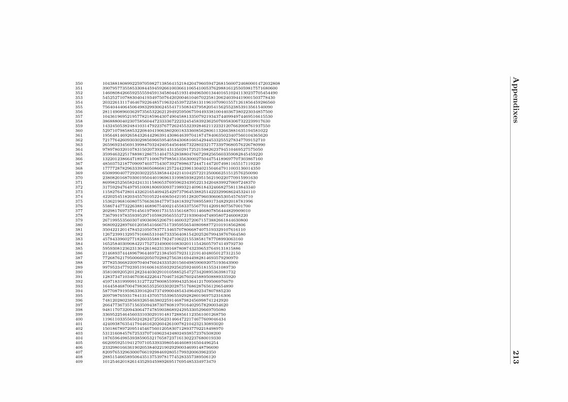
App

endix

es

213

350 104388180899225970598271385641521842047960594726815600724680001472032808351 39079577355853308445945926610036611065410053762988161255059817571680600352 14608084266592555594591345804451931494965001344016510241130237705454490353 5452527107883040419349750764202004610467022581206240394419001503778430354 2032261311746467922648571963245397225813119610709015571261856459286560355 756404440645064983299306245541715083437958205415625523853913561540090356 281149089603629735653226212949259506759449338100440367380223034857500357 104361969521957782185964307490458813350792193437440994974469516615530358 38688800402307585604472333367222324545839236250769583067322239917630359 14324505382484103147922376772624553239284621122321207662008761937550360 5297107985885322084041906380200183336085628061132663881635194581022361 1956481469265843264429639143086463970418747840635023407560104365620362 721776426093030298569665954058430681665429445332555278347709152710363 265969234569139984703242405445646673228023217733979680576226780990364 97897803201078315020739361431350291725215982623794510469527575050365 35994632251788981286751404755283880476672982565603359082845459220366 13220123866471893711006797985613563000275044754189697707303867160367 4850375218770909740377543073927898637244714472074981165517119220368 1777728782963339380508668125724423961304021504647911003136014350369 650899040772920302225538584424214104257221250066251512576250090370 238082016870300195044019696131998593822951562190220770915991630371 86998252565824241311580653769596234395221342048399270697248370372 31759294764979510081806930937198932140961843246682758113843340373 11582764728014326216540942542973796453882514223299686245324110374 4220254518203455701052244065042195128207960306065305457659710375 1536219681608075766363847797348183927089558917348292018781996376 558674477322638814689675400214558337556770142091807567001700377 202981769737914561979001731551561687011466807856444829909010378 73679919783593952971059829565552721939040474895807246008220379 26719955356030749036965206791460032720671573882661844630800380 9680922289760120585416667517395955654080988772101918562806381 3504221201478452105078377134657078066874075193329107616110382 1267239913295791686531046733356408154202526799438767664580383 457843396027718260355881782471062215538581787708993063160384 165258403090842217527234900010830201115426057974149792730385 59593081236231304261862313916878087432396537649131815886386 21468937444896796446972138450579231121914048050127312150387 7726876217950066020507028827563816944982814693579290970388 2778253668220970404766243335201560498590692075193643900289 997952347792395191606163593292562592469518155341089730390 358106920520128234403029101058852547273420895363981732391 128373471034670364222641704671626760245889508889335920392 45971831999991312772278008559994325364121709506976670393 16445846870047983653525033020287517686287656129654890394 5877087919596339162047374990048543496492347807885230395 2097987659317841314370575539655929282801969752316306396 748120280238569326546380225914687982456998741242920397 266477367357156350943873078081979164029578290034620398 94811707320943064774785903868924295330529669705080399 33695225464560331030291914817288561123561001268750400 11961103355650242824725562314664722174677609046434401 4240938763541794461620260426100782104232130893020402 1501867897209514546756012058307128937792218498970403 531216084576725337071696234248024938572376508200404 187659649853938590532176587237161302237680019330405 66209592519412707105339339805464608916504496254406 23329801663619020538402219029290034699148796690407 8209765329630007661929846928051799320063962350408 2885154665895064351375397817745283357389506120409 1012546201826143529345989269517695485334973470

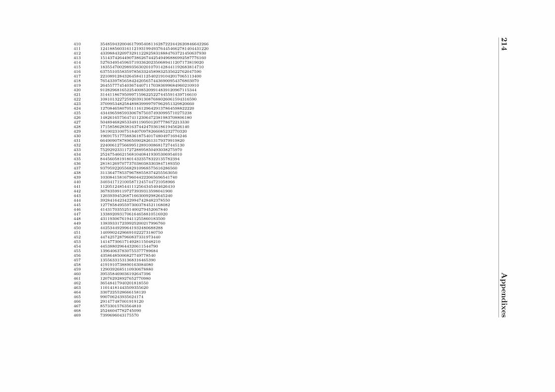
214

Ap

pendix

es

410 354859432004617995408116287222442620846642266411 124188560316112193199493764454662781404431220412 43398843209732911228258318884763721450637930413 15143742644907386267442549496886992587776160414 5276349545965719336202350689411207173819020415 1835547002989356302010701428441192683814710416 637551055835978563324589832535622762047590417 221089128432645841125402191042017065113400418 76543397856584242056574436900954376803070419 26455777454036744071170383699684960210910420 9128296816522540085209914839120967115344421 3144118679509971596225227445591439716610422 1081013227259203913087688026061594316590423 370995348258489839999797962951329820660424 127084658070511161296429137864598822220425 43449659859330678750374930995710275238426 14826165756474112306472381983708806180427 5048946828533491190501207778672213330428 1715858628381637442470361861945626140429 581902310075184070978266085232770320430 196917517758836187540174804971694246431 66490907878965090282613179379919820432 22400612756699512891008681727445130433 7529292331172728895850493038275970434 2524754662156810408419305306954010435 844560581918014323578322135782394436 281812697077370380383303847189350437 93795922055682910968575616286560438 31136477853796788558374255563050439 10308415816796044222065696541740440 3403417121005871245744721058966441 1120512485441112564345404626410442 367835991197273939313598041900443 120393945268716630092982645240444 39284164234229947428482378550445 12778584955973003784521168082446 4143170355251400279452067840447 1338920931706164658810516920448 431193067619411255860183500449 138393317239925200217996760450 44253449299641932480688288451 14099024296691022273180750452 4474257287960837331973440453 1414773061714928115048210454 445388029644320611544790455 139640637830755377789684456 43586485006827749778540457 13556331531368316465390458 4191910738890163084080459 1290392685110930678880460 395358469036192647396461 120762928927652770980462 36548417940201818550463 11014181443509355620464 3307225528666158120465 990706243935624174466 291477487001919120467 85733015763564810468 25246047782745090469 7399696043175570

App

endix

es

215

470 2086326646454628471 599101822655130472 174116764660860473 49520192753070474 12988896122430475 3699657010116476 1076263554150477 288545344020478 66595291470479 20069636040480 5894444562481 1379596770482 255032280483 97330650484 27450810485 4768380486 603600487 428220488 95850489 8730490 540491 1530492 180493 0494 0495 3

Bibliography

[1] Abe, R. (1967). Logarithmic singularity of specific heat near the transition pointin the Ising model. Progress of Theoretical Physics, 37(6):1070–1079.

[2] Andrews, G. E., Baxter, R. J., and Forrester, P. J. (1984). Eight-vertex SOSmodel and generalized Rogers-Ramanujan-type identities. Journal of StatisticalPhysics, 35(3):193–266.

[3] Ashkin, J. and Teller, E. (1943). Statistics of two-dimensional lattices with fourcomponents. Phys. Rev., 64:178–184.

[4] Atkins, P. W. and de Paula, J. (2006). Physical Chemistry. W.H. Freeman &Co., New York, seventh edition.

[5] Baxter, R. J. (1973). Potts model at the critical temperature. Journal of PhysicsC: Solid State Physics, 6(23):L445.

[6] Baxter, R. J. (1995). Solvable model in Statistical Mechanics, from Onsageronward. Journal of Statistical Physics, 78(1-2):7–16.

[7] Baxter, R. J. (2007). Exactly Solved Models in Statistical Mechanics. CourierDover Publications, third edition.

[8] Baxter, R. J. (2011). Onsager and Kaufmans calculation of the spontaneousmagnetization of the Ising model. Journal of Statistical Physics, 145(3):518–548.

[9] Bhanot, G. and Sastry, S. (1990). Solving the Ising model exactly on a 5x5x4lattice using the connection machine. Journal of Statistical Physics, 60:333–346.

[10] Bowley, R. and Sanchez, M. (1996). Introductory Statistical Mechanics. Oxford:Clarendon.

[11] Bragg, W. and Bragg, W. (1915). X Rays and Crystal Structure. Bell.

[12] Brush, S. G. (1967). History of the Lenz-Ising model. Rev. Mod. Phys., 39:883–893.

[13] C, M. (2000). Matrix analysis and applied linear algebra. SIAM.

217

Bibliography Bibliography

[14] Callen, H. (1985). Thermodynamics and an Introduction to Thermostatistics.Wiley.

[15] Chandler, D. (1987). Introduction to Modern Statistical Mechanics. OxfordUniversity Press.

[16] Chen, C.-N., Hu, C.-K., and Wu, F. (1996). Partition function zeros of thesquare lattice Potts model. Physical review letters, 76(2):169.

[17] Cipra, B. A. (1987). An introduction to the ising model. The AmericanMathematical Monthly, 94(10):937–959.

[18] De Graef, M. and McHenry, M. E. (2007). Structure of Materials: AnIntroduction to Crystallography, Diffraction and Symmetry. CambridgeUniversity Press, first edition.

[19] Diestel, R. (2006). Graph Theory. Electronic library of mathematics. Springer.

[20] Domb, C. (1949). Order-disorder statistics. I. Proceedings of the Royal Society ofLondon A: Mathematical, Physical and Engineering Sciences, 196(1044):36–50.

[21] Einhorn, M. B., Savit, R., and Rabinovici, E. (1980). A physical picture for thephase transitions in Zn symmetric models. Nuclear Physics B, 170(1):16 – 31.

[22] Elitzur, S., Pearson, R. B., and Shigemitsu, J. (1979). Phase structure of discreteabelian spin and gauge systems. Phys. Rev. D, 19:3698–3714.

[23] Enting, I. and Wu, F. (1982). Triangular lattice Potts models. Journal ofStatistical Physics, 28(2):351–373.

[24] Feldmann, H., Guttmann, A. J., Jensen, I., Shrock, R., and Tsai, S.-H.(1998a). Study of the Potts model on the honeycomb and triangular lattices:Low-temperature series and partition function zeros. Journal of Physics A:Mathematical and General, 31(10):2287.

[25] Feldmann, H., Shrock, R., and Tsai, S.-H. (1998b). Complex-temperaturepartition function zeros of the Potts model on the honeycomb and kagomelattices. Phys. Rev. E, 57:1335–1346.

[26] Fisher, M. E. (1965). The nature of critical points. In Britten, W. E., editor,Lectures in Theoretical Physics, volume 7c, pages 1–159. University of ColoradoPress, Boulder.

[27] Ford, I. (2013). Statistical Physics: An Entropic Approach. John Wiley andSons, Ltd.

[28] Geim, A. K. and Novoselov, K. S. (2007). The rise of graphene. Nature Materials,6(3):183–191.

Bibliography 219

[29] Ghulghazaryan, R. G. and Ananikian, N. S. (2003). Partition function zeros ofthe one-dimensional Potts model: the recursive method. Journal of Physics A:Mathematical and General, 36(23):6297.

[30] Gibbs, J. W. (1902). Elementary Principles in Statistical Mechanics. YaleUniversity Press. Reprinted by Dover, New York, 1960.

[31] Hales, T. (2012). Dense Sphere Packing, A Blueprint for Formal Proof.Cambridge University Press.

[32] Hamermesh, M. (1962). Group theory and its applications to physical problems.Addison-Wesley, Reading, Massachusetts. Reprinted by Dover, New York, 1989.

[33] Hill, T. (1960). An Introduction to Statistical Thermodynamics. Addison-Wesleyseries in chemistry. Dover Publications.

[34] Hintermann, A., Kunz, H., and Wu, F. Y. (1978). Exact results for the Pottsmodel in two dimensions. Journal of Statistical Physics, 19(6):623–632.

[35] Huang, K. (1987). Statistical Mechanics. John Wiley & Sons Ltd., secondedition.

[36] Huse, D. A. (1984). Exact exponents for infinitely many new multicritical points.Phys. Rev. B, 30:3908–3915.

[37] Ising, E. (1925). Beitrag zur Theorie des Ferromagnetismus. Zeitschrift furPhysik, 31:253–258.

[38] Katsura, S. (1967). Distribution of roots of the partition function in the complextemperature plane. Progress of Theoretical Physics, 38(6):1415–1417.

[39] Katsura, S. and Ohminami, M. (1972). Distribution of zeros of the partitionfunction of the lattice gases of fisher and of temperley. Physics Letters A,40(4):283 – 284.

[40] Kaufman, B. (1949). Crystal Statistics. II. Partition function evaluated by spinoranalysis. Phys. Rev., 76:1232–1243.

[41] Kittel, C. (2004). Introduction to Solid State Physics. Wiley, eighth edition.

[42] Kogut, J. B. (1979). An introduction to lattice gauge theory and spin systems.Rev. Mod. Phys., 51:659–713.

[43] Kosterlitz, J. M. and Thouless, D. J. (1973). Ordering, metastability andphase transitions in two-dimensional systems. Journal of Physics C: Solid StatePhysics, 6(7):1181–1203.


[44] Kramers, H. A. and Wannier, G. H. (1941a). Statistics of the two-dimensionalferromagnet. Part I. Phys. Rev., 60:252–262.

[45] Kramers, H. A. and Wannier, G. H. (1941b). Statistics of the two-dimensionalferromagnet. Part II. Phys. Rev., 60:263–276.

[46] Krieger, M. H. (1996). Constitutions of Matter: Mathematically Modelingthe Most Everyday of Physical Phenomena. Cinema and Modernity Series.University of Chicago Press.

[47] Kubo, R. (1943). An analytic method in Statistical Mechanics. Busseiron-kenkyu, 1:1–13.

[48] Landau, L. and Lifshitz, E. (1968). Statistical Physics, volume 5. PergamonPress, second revised and enlarged edition.

[49] Lane, S. (1998). Categories for the Working Mathematician. Graduate Texts inMathematics. Springer New York.

[50] Lee, T. D. and Yang, C. N. (1952). Statistical theory of equations of state andphase transitions II. Lattice gas and Ising model. Phys. Rev., 87:410–419.

[51] Maillard, J. M. and Rammal, R. (1983). Some analytical consequences of theinverse relation for the Potts model. Journal of Physics A: Mathematical andGeneral, 16(2):353.

[52] Mandl, F. (1988). Statistical Physics. John Wiley & Sons Ltd., second edition.

[53] Marsden, J. and Hoffman, M. (1999). Basic Complex Analysis. W. H. Freeman.

[54] Martin, P. (1982). Discrete abelian gauge models on small three-dimensionallattices. Nuclear Physics B, 205(2):301–312.

[55] Martin, P. P. (1983). Finite lattice Z(3) models in two and three dimensions.Nuclear Physics B, 225(4):497–504.

[56] Martin, P. P. (1985). Potts models and dichromatic polynomials. In GiacomoM. D′Ariano and Mario Rasetti, editors, Integrable Systems in StatisticalMechanics, pages 129–142. World Scientific.

[57] Martin, P. P. (1988). Exact finite lattice results for Zn symmetric spin models.J. Phys. A: Math. Gen, 21:4415–4421.

[58] Martin, P. P. (1991). Potts Models and Related Problems in StatisticalMechanics, volume 5. World Scientific Pub Co Inc.

[59] Martin, P. P. (2000). Zeros of the partition function for the triangular latticethree-state Potts model II. http://www1.maths.leeds.ac.uk/~ppmartin/

ZEROS/pdf/q3tri2x.pdf.

Bibliography 221

[60] Martin, P. P. and Maillard, J. M. (1986). Zeros of the partition function for thetriangular lattice three-state Potts model. Journal of Physics A: Mathematicaland General, 19(9):L547.

[61] Matveev, V. and Shrock, R. (1996). Complex-temperature properties of the two-dimensional Ising model for nonzero magnetic field. Phys. Rev. E, 53:254–267.

[62] McCoy, B. M. and Wu, T. T. (1973). The Two-dimensional Ising Model. HarvardUniversity Press.

[63] McCoy, N. H. and Janusz, G. J. (2001). Introduction to Abstract Algebra.Harcout Academic Press, 6 edition.

[64] McKie, D. and McKie, C. (1974). Crystalline Solids. Thomas Nelson & Sons,Limited.

[65] McQuarrie, D. A. (2000). Statistical Mechanics. University Science Books.

[66] Montroll, E. W. (1941). Statistical Mechanics of nearest neighbor systems. TheJournal of Chemical Physics, 9(9):706–721.

[67] Montroll, E. W. (1942). Statistical Mechanics of nearest neighbor systems II.General theory and application to twodimensional ferromagnets. The Journalof Chemical Physics, 10(1):61–77.

[68] Newell, G. F. and Montroll, E. W. (1953). On the theory of the Ising model offerromagnetism. Rev. Mod. Phys., 25:353–389.

[69] Ninio, F. (1976). A simple proof of the perron-frobenius theorem for positivesymmetric matrices. Journal of Physics A: Mathematical and General, 9(8):1281.

[70] Niss, M. (2005). History of the Lenz-Ising model 1920-1950: From ferromagneticto cooperative phenomena. Archive for History of Exact Sciences, 59(3):267–318.

[71] Novoselov, K. S., Jiang, D., Schedin, F., Booth, T. J., Khotkevich, V. V.,Morozov, S. V., and Geim, A. K. (2005). Two-dimensional atomic crystals.Proceedings of the National Academy of Sciences of the United States of America,102(30):10451–10453.

[72] Oguchi, T. (1949). Statistics of the three-dimensional ferromagnet. Phys. Rev.,76:1001–1001.

[73] Oguchi, T. and Taguchi, Y. (1986). Transfer matrix and finite-size scaling forthe Ising model on two- and three-dimensional lattices. Progress of TheoreticalPhysics Supplement, 87:23–32.


[74] Ono, S., Karaki, Y., Suzuki, M., and Kawabata, C. (1967). Statistical mechanicsof three - dimensional finite Ising model. Physics Letters A, 24(12):703–704.

[75] Onsager, L. (1944). Crystal Statistics. I. A two-dimensional model with anorder-disorder transition. Phys. Rev., 65:117–149.

[76] Papoulis, A. and Pillai, S. (2001). Probability, Random Variables and StochasticProcesses with Errata Sheet. McGraw-Hill Series in Electrical and ComputerEngineering. McGraw-Hill.

[77] Pearson, R. B. (1982). Partition function of the Ising model on the periodic4x4x4 lattice. Phys. Rev. B, 26:6285–6290.

[78] Peierls, R. (1936). On Ising’s model of ferromagnetism. MathematicalProceedings of the Cambridge Philosophical Society, 32:477–481.

[79] Potts, R. B. (1952). Some generalized order-disorder transformations.Mathematical Proceedings of the Cambridge Philosophical Society, 48:106–109.

[80] Priestley, H. (2003). Introduction to Complex Analysis. OUP Oxford.

[81] Quarteroni, A., Sacco, R., and Saleri, F. (2007). Numerical Mathematics.Springer, Berlin.

[82] Sands, D. E. (1993). Introduction to Crystallography. Courier DoverPublications.

[83] Savit, R. (1980). Duality in field theory and statistical systems. Rev. Mod.Phys., 52:453–487.

[84] Schneider, H. and Barker, G. (1968). Matrices and linear algebra. Holt, Rinehartand Winston.

[85] Shackelford, J. F. (2000). Introduction to Materials Science for Engineers.Prentice-Hall, Inc, fifth edition.

[86] Stephenson, J. (1987). On the density of partition function temperature zeros.Journal of Physics A: Mathematical and General, 20(13):4513.

[87] Swendsen, R. (2012). An Introduction to Statistical Mechanics andThermodynamics. Oxford Graduate Texts. OUP Oxford.

[88] Syozi, I. (1972). Transformation of Ising models. In Domb, C. and Green, M. S.,editors, Phase Transitions and Critical Phenomena, volume 1, pages 269–329.Academic Press, London.

[89] Ter Haar, D. (1952). Statistics of the three-dimensional ferromagnet: II.Comparison of various approximation methods. Physica, 18(11):836–840.

Bibliography 223

[90] Ter Haar, D. (1953). Statistics of the three-dimensional ferromagnet III. Somenumerical results. Physica, 19(112):611–614.

[91] Thomas, G. and Goringe, M. (1981). Transmission Electron Microscopy ofMaterials. TechBooks, Fairfax.

[92] Valani, Y. P. (2011). On the Partition Function for the Three-dimensional Isingmodel. PhD thesis, Engineering and Mathematical Sciences, City University,London.

[93] Villain, J. (1975). Theory of one- and two-dimensional magnets with an easymagnetization plane. II. the planar, classical, two-dimensional magnet. J. Phys.France, 36(6):581–590.

[94] Wannier, G. (1966). Statistical Physics. Dover Books on Physics. DoverPublications.

[95] West, D. (2001). Introduction to Graph Theory. Featured Titles for GraphTheory Series. Prentice Hall.

[96] Wilde, R. E. and Singh, S. (1998). Statistical Mechanics: Fundamentals andmodern applications. John Wiley & Sons Ltd.

[97] Woolfson, M. M. (1997). An Introduction to X-ray Crystallography, SecondEdition. Cambrigde University Press, second edition.

[98] Wu, F. Y. (1982). The Potts model. Rev. Mod. Phys., 54:235–268.

[99] Yang, C. N. and Lee, T. D. (1952). Statistical theory of equations of state andphase transitions I. Theory of condensation. Phys. Rev., 87:404–409.

[100] Yang, H., Hernandez, Y., Schlierf, A., Felten, A., Eckmann, A., Johal, S.,Louette, P., Pireaux, J.-J., Feng, X., Mullen, K., Palermo, V., and Casiraghi,C. (2013). A simple method for graphene production based on exfoliation ofgraphite in water using 1-pyrenesulfonic acid sodium salt. Carbon, 53:357–365.

[101] Yeomans, J. M. (1992). Statistical Mechanics of Phase Transitions. OxfordUniversity Press.

[102] The GNU Multiple Arithmetic Library. (2016). Retrieved fromhttps : //gmplib.org.

analytic properties of potts and ising model partition

Documents