analytical and simulation models for evaluating …
TRANSCRIPT

The Pennsylvania State University
The Graduate School
Harold and Inge Marcus
Department of Industrial and Manufacturing Engineering
ANALYTICAL AND SIMULATION MODELS FOR EVALUATING CASH-FLOW
BULLWHIP IN SUPPLY CHAINS
A Thesis in
Industrial Engineering
by
HyunJong Shin
2013 HyunJong Shin
Submitted in Partial Fulfillment
of the Requirements
for the Degree of
Master of Science
December 2013
The thesis of HyunJong Shin was reviewed and approved* by the following:
Vittal Prabhu
Professor, Department of Industrial and Manufacturing Engineering
Thesis Advisor
Ravi Ravindran
Professor, Department of Industrial and Manufacturing Engineering
Chair, Enterprise Integration Consortium
Paul Griffin
Professor, Department of Industrial and Manufacturing Engineering
Head of the Department of Industrial and Manufacturing Engineering
*Signatures are on file in the Graduate School

iii
ABSTRACT
Inventory bullwhip in supply chain can have numerous adverse consequences and has
been widely investigated over the last several years. Recent research has begun to investigate the
plausibility bullwhip in cash-flow and has focused on developing theoretical models using
analytical and simulation tools. This thesis extends these theoretical investigations by studying
the effect of cash collection size and the variance in cash collection. In particular, a series of
designed experiments are conducted using computer simulation of a four-tier supply chain in
which cash collection is treated as a random variable. From the observation of these experiments,
the size of cash collection is either irrelevant or marginally relevant to the cash flow bullwhip
effect. Moreover, analytical models are developed to characterize the effect of variance in cash
collection when it is has a normal or exponential distribution. No matter which distribution is
assumed for the cash collection, the models tend to overestimate the cash flow bullwhip. When
the cash collection follows normal distribution, the model over estimates cash flow bullwhip by
approximately 30%. Whereas the model over estimates cash flow bullwhip by approximately
150% when the cash collection follows exponential distribution

iv
TABLE OF CONTENTS
List of Figures .......................................................................................................................... v
List of Tables ........................................................................................................................... vi
Acknowledgements .................................................................................................................. vii
Chapter 1 Introduction ............................................................................................................. 1
Chapter 2 Literature Review .................................................................................................... 4
2.1. Supply Chain Management ....................................................................................... 4
2.2 Bullwhip Effect in Supply Chain ............................................................................... 4
2.3. Cash Flow Bullwhip Effect in Supply Chain ............................................................ 6
2.4. Extended Beer Game Model .................................................................................... 6
Chapter 3 An Effect of Cash Collection Size on Supply Chain Cash Flow............................. 9
3.1. Motivation and Problem ............................................................................................ 9
3.2. Methodology ............................................................................................................. 10
3.3. Result ........................................................................................................................ 12
3.3.1. CV(𝐏𝐚𝐲𝐦𝐞𝐧𝐭𝑹𝒆𝒕𝒂𝒊𝒍𝒆𝒓) .............................................................................. 13
3.3.2. CV(𝐏𝐚𝐲𝐦𝐞𝐧𝐭𝑫𝒊𝒔𝒕𝒓𝒊𝒃𝒖𝒕𝒐𝒓) ........................................................................ 14
3.3.3. CV(𝐏𝐚𝐲𝐦𝐞𝐧𝐭𝒎𝒂𝒏𝒖𝒇𝒂𝒄𝒕𝒖𝒓𝒆𝒓) .................................................................. 15
3.3.4. CV(𝐏𝐚𝐲𝐦𝐞𝐧𝐭𝑺𝒖𝒑𝒑𝒍𝒊𝒆𝒓) .............................................................................. 16
3.4. Conclusive Remarks ................................................................................................. 17
Chapter 4 An effect of Cash Collection Ratio Variation on Supply Chain Cash Flow ........... 20
4.1. Motivation and Problem ............................................................................................ 20
4.2. Methodology ............................................................................................................. 20
4.3. Derivation and Result ................................................................................................ 21
4.3.1. Normal Distribution and Exponential Distribution ........................................ 24
4.3.3. Family of Normal Distribution ....................................................................... 29
4.4. Conclusive Remarks ................................................................................................. 31
Chapter 5 Summary and Future Research ................................................................................ 32
5.1. Summary ................................................................................................................... 32
5.2. Future Research ......................................................................................................... 33
References ................................................................................................................................ 35
Appendix Matlab Code for Extended Beer Distribution Game Model ........................... 37
v
LIST OF FIGURES
Figure 2 - 1 Supply Chain ........................................................................................................ 4
Figure 2 - 2 Bullwhip Effect .................................................................................................... 5
Figure 2 - 3 Supply Chain Model with Cash Flow .................................................................. 7
Figure 2 - 4 Normalized Payments for Supply Chain Member vs Time ................................. 8
Figure 3 - 1 Supply Chain ........................................................................................................ 9
Figure 4 - 1 Comparison between Simulation and Analytic (Normal) Result ......................... 27
Figure 4 - 2 Comparison between Simulation and Analytic (Exponential) Result .................. 28
Figure 4 - 3 Comparison of C.V. ............................................................................................. 28
Figure 4 - 4 Family of Normal Distribution ............................................................................. 29
Figure 4 - 5 Comparison between Family of Normal Dis. and Exponential Dis. .................... 30
vi
LIST OF TABLES
Table 3 - 1 How cash flow bullwhip effect can be compared to bullwhip effect .................... 10
Table 3 - 2 Decision Variables for the DOE ............................................................................ 11
Table 3 - 3 Design of Experiment ............................................................................................ 12
Table 3 - 4 Independent Variables included in the Regression Model for Retailer ................. 13
Table 3 - 5 Independent Variables included in the Regression Model for Distributor ............ 14
Table 3 - 6 Independent Variables included in the Regression Model for Manufacturer ........ 15
Table 3 - 7 Independent Variables included in the Regression Model for Supplier ................ 16
Table 3 - 8 Comparison between Liu’s and Shin’s DOE Model ............................................. 18
Table 3 - 9 Variables included in the Regression Models ....................................................... 18
Table 4 - 1 Coefficient of variation of Oj ................................................................................. 26
Table 4 - 2 Family of Normal Distribution with Mean of 0.45 ................................................ 30
vii
ACKNOWLEDGEMENTS
I would like to give thanks to people who help and encourage me to complete this thesis.
In the first, I would like to express my deepest appreciation to Dr. Prabhu, my great adviser. His
care and patience encouraged me to complete this work. Moreover his profound insight and great
advice and guidance helped me to see supply chain in new perspective. Without his guidance and
encouragement, this thesis, for sure, would not be completed. I also would like to thank to Dr.
Ravindran who gladly spent his time to thoroughly review this thesis. I also appreciate all support
of members of DISCRETE Lab.
I thank to my family in Korea (my father, my mother and all relatives), and in United
States (my sister, and my brother in law). I appreciate your supports and especially your prayers.
Without your support and prayers, would stop in the middle of this journey. In addition, I thank
to all of my friends in State College (especially, JY Ha, EH Woo, EK Han) and in all over the
world (especially HS Cho, CM Yeo, DH You, YD Ha, YJ Lee, JW Yoo, JM Ahn, TK Kim,
DS Lee, YM Kweon, and CL Park,)
Lastly but most importantly, thanks God who worked before me and has brought me
to this far since when I was born. I live by your grace and mercy!

1
Chapter 1
Introduction
Many supply chain management textbooks teach that there are three components in
supply chain management: goods, information and cash (Handfield, 1999, Fawcett, 2006 and
Bernd 2002). However, for many years, not only practitioners but also many researchers have
only focused on the flow of physical goods and information in supply chain. The study of cash
flow is neglected. Consequently, average inventory level of a firm was reduced by 35% while
account receivables were reduced by only 16% for the last 20 years, according to the report of the
TradeBeam by Hausman in 2009.
However, the studied trend has slowly changed from the flow of physical goods and
information to the flow of cash in supply chain, as the world recently faced its worst financial
crisis in history (Kirkup, 2011). During the recent financial crisis, financial institutions were
reluctant to lend money and companies were afraid of running their business with credit because
financial asset’s nominal value was dropped abruptly (“Worldbank.org”, 2013). As a result,
companies, especially small and medium sized enterprises, which do not hold adequate cash to
pay what they owed, tried to extend their account payable term and shorten their account
receivable term at the same time in order to stay in business. Unfortunately all of these attempts
did not prevent them from going bankrupt during this time (“Worldbank.org”, 2013). Therefore,
survived companies and researchers realize the importance of holding sufficient cash on hand and
cash flow during and after unstable economic condition.
While practitioners realize the importance of the cash due to the financial crisis, the field
of supply chain management also faced new paradigm due to the progress of information

2
technology. In the past, the role of supply chain management was limited. The researchers in the
field of supply chain management focused on production or logistic aspects of business as it is
mentioned above. However, as the information technology progresses, the role of supply chain
management is expanded to all aspects of business such as marketing and finance (Camerinelli,
2009). As a result, there are few papers that suggest integration between supply chain
management and cooperate cash management. For example, in 2006 Hofmann conceptually
suggested a way to manage working capital with collaboration of players in supply chain.
Not until recently, the study of cash flow in supply chain is proposed. In 2010,
Sasisekaran reported the prominence of the demand forecasting on the cash flow in supply chain.
Sasisekaran concluded based on the VBA simulation that, when the forecasting model is correctly
implemented, there is a possibility to free up large amounts of capitals which could go into new
investment (Saisekaran, 2010). Moreover, in 2013, He was focused on studying cash flow
forecasting in different economic conditions. He tried to find out how the customer payment time
which probability is represented by Weibull distribution, affects the proper value of working
capital requirement of supply chain members (He, 2013). In addition, Tangsucheeva proposed a
new cash collection prediction model which was built by combining Markov Chain and
exponential smoothing forecasting technique. This new attempt tries to help SMEs’ cash flow by
improving the accuracy of cash collection prediction rate (Tangsucheeva, 2013).
Meanwhile, others focused on the cash flow bullwhip effect in supply chain. In 2011, Liu
proposed a simple model which extended the beer distribution game model by introducing a cash
flow component in the model (Liu, 2011). In his dissertation, Liu proposed the existence of cash
flow bullwhip effect using the model he developed. In addition, he proposed another model which
illustrates the effect of payment decision rule on cash flow in supply chain (Liu, 2011). While Liu
was focused on studying existence of cash flow bullwhip effect using the beer distribution game
model, Tangsucheeva proposed cash flow bullwhip effect in a different perspective
3
(Tangsucheeva, 2013). Instead of using the beer distribution game, Tangsucheeva proposed the
existence of cash flow bullwhip effect using an analytical model which is derived from the Cash
Conversion Cycle. In addition, he proposed that 20% of cash flow bullwhip effect is contributed
by the bullwhip effect (Tangsucheeva, 2013).
The main contribution of both Liu’s thesis and Tangsucheeva’s paper is that they both
identified the cash flow bullwhip effect in supply chain. Thus, it is natural to pay attention to the
drivers of cash blow bullwhip effect like decades ago, researchers had focused on studying the
drivers of the bullwhip effect and how to mitigate this phenomenon, since bullwhip effect has
been identified.
In Liu’s thesis, he designed experiments to identify factors that affect the cash flow
bullwhip effect. More specifically speaking, he focused on the finding impact of moving average
term which is used in demand forecast and cash collection forecast on cash-flow bullwhip effect.
However, he did not put much attention on impact of cash collection ratio itself on cash flow
bullwhip effect, even though cash collection is the only financial component used in the model.
Thus, in this thesis, the effect of cash collection ratio is studied in depth based on Liu’s model: (1)
how the size of cash collection affects the cash flow bullwhip effect, and (2) how the variation of
cash collection ratio affects the cash flow bullwhip effect.
And the rest of the thesis is organized as follows: Chapter 2 provides summary of
bullwhip effect by introducing some important papers since the existence of bullwhip effect was
detected. At the same time the concept of cash flow bullwhip effect is introduced. Furthermore,
overview of Liu’s model is presented in detail. In Chapter 3, a problem, “how the size of cash
collection ratio affects the cash flow bullwhip effect is studied via Design of Experiment. The
details of the methodology are explained in Chapter 3. Chapter 4 proposes an analytic model to
determine the variation of cash collection ratio effect on the cash flow bullwhip effect. Lastly, in
chapter 5, the conclusive remarks and direction for future works are discussed.

4
Chapter 2
Literature Review
2.1. Supply Chain Management
Since late 1990s, a term called Supply Chain Management became popular (Cooper,
1997). The number of conference sessions which titles contains “supply chain” increase from
13.5% to 22.4% in two years at the annual conference of the Council of Logistics Management
(Cooper, 1997). However, the definition of supply chain management was not completely
determined by researchers. During late 1990s, the concept of supply chain management is
something that is similar to logistic management (Cooper, 1997).
Figure 2 - 1 Supply Chain
Therefore, the more comprehensive definition was needed. In 2001, Mentzer defines
supply chain as “a set of three or more entities (organizations or individuals) directly involved in
the upstream and downstream flows of products, services, finances, and/or information from a
source to a customer.”
2.2 Bullwhip Effect in Supply Chain
The phenomenon in which product order size is amplified as it goes to the upper player in
the supply chain is called “Bullwhip Effect” (Bernd, 2002) as it is shown in the Figure 2 – 2.
Supplier (j=5)
Mfg. (j=4)Distributor
(j=3)Retailer (j=2)
Cutomer (j=1)

5
Since this phenomenon was identified first in 1989, researchers focused on studying causes or
drivers of the bullwhip effect and how to mitigate this phenomenon.
Figure 2 - 2 Bullwhip Effect
In 1989, Sterman successfully introduced and identified the existence of bullwhip effect
using Beer Distribution Game. In the same year, Burbidge also introduced the bullwhip effect by
describing cause or reason of existence. He proposed that bullwhip effect exists in the supply
chain because of following reasons: deluded information and delays of materials.
After Burbidge’s attempt to explain the cause of the bullwhip effect, many of other
researchers also focused on explaining causes of the bullwhip effect. For example, Lee et al in
1997 listed four reasons in his paper: demand forecast update, batch order, fluctuation in price
and rationing game.
While some researchers had focused on identifying causes of the bullwhip effect, some
had focused on influences of bullwhip effect. For example, researchers reported that bullwhip
effect brings negative influences to the supply chain such as excessive inventory level,
backorders, uncertainty in production planning, and stock out (Chen, 1998, Jones, 2000 and Lee
et al, 2004).
After identifying the causes of the phenomenon, researchers had put their efforts on
quantifying the bullwhip effect. In 2000 Chen was able to quantify the bullwhip effect for simple
supply chain. After Chen, much more sophisticated supply chain was quantified by other
researchers such as Kim in 2006 and Fioriolli in 2008

6
2.3. Cash Flow Bullwhip Effect in Supply Chain
Not many papers about the cash flow bullwhip effect exist because the term, cash flow
bullwhip effect is newly introduced by Tangsucheeva and Prabhu in 2013. Prior to Tangsucheeva
and Prabhu, a similar work can be found in 2011.
In 2011, Liu introduced a concept which states that a similar effect to bullwhip effect
exists in supply chain cash flow. In Liu’s paper, he extended Chatfield’s beer game by
introducing a cash flow component to the model. In addition, Liu also suggested the metric which
can capture the cash flow bullwhip effect in supply chain, which is Coefficient of Variation of
Payment.
While Liu’s thesis used coefficient of variation of payment to illustrate cash flow
bullwhip effect in the supply chain, Tangsucheeva and Prabhu used different approaches to
explain the cash flow bullwhip effect in the supply chain. Tangsucheeva and Prabhu proposed
that inventory bullwhip effect leads to cash flow bullwhip effect and it can be explained by using
Cash Conversion Cycle as the metric. According to Tangsucheeva and Prabhu, approximately
20% of cash flow bullwhip effect is due to the inventory bullwhip effect (Tangsucheeva and
Prabhu, 2013).
2.4. Extended Beer Game Model
In order to see whether the financial factors, such as payment and collection of cash
uncertainty, makes impact on the cash flow bullwhip effect, Liu extended the popular model,
beer distribution game by introducing a financial component to the model.

7
In this model, there are five players: Supplier, Manufacturer, Distributor, Retailer and
Customer. The orders and cash flows upstream the supply chain while the goods flow
downstream the supply chain as it is shown in Figure 2 – 3.
Figure 2 - 3 Supply Chain Model with Cash Flow
In Liu’s extended model, the inventory replenishment policy is set to be order-up-to
policy and expressed as following:
Ot = 𝐿�̅� + 𝑘𝜎 − (𝑖𝑛𝑣𝑒𝑛𝑡𝑜𝑟𝑦 𝑜𝑛 ℎ𝑎𝑛𝑑 𝑎𝑡 𝑡 + 𝑖𝑛𝑣𝑒𝑛𝑡𝑜𝑟𝑦 𝑜𝑛 𝑜𝑟𝑑𝑒𝑟 𝑎𝑡 𝑡 − 𝑏𝑎𝑐𝑘𝑜𝑟𝑑𝑒𝑟 𝑎𝑡 𝑡)
where, L is lead time and �̅� is demand mean over the lead time which is updated by moving
average forecasting method.
Liu introduced a simple rule for payment decision under which a player expects to pay
more if a players expect to collect more from its customer (Liu, 2011). Specifically in each time,
each member calculates how much they are going to collect from its downstream player. This is
expressed in the following equation:
𝛽𝑡 = {
𝑐𝑜𝑙𝑙𝑒𝑐𝑡𝑖𝑜𝑛 𝑓𝑜𝑟 𝑠𝑎𝑙𝑒 𝑎𝑡 (𝑡 − 2)
𝑠𝑎𝑙𝑒𝑠 𝑎𝑡 (𝑡 − 2), |𝑖𝑓 𝑠𝑎𝑙𝑒𝑠 𝑎𝑡 (𝑡 − 2) ≠ 0
0 , |𝑖𝑓 𝑠𝑎𝑙𝑒𝑠 𝑎𝑡 (𝑡 − 2) = 0
In addition, the payment decision of each player is as follows:
𝑃𝐴𝑌𝑡+1 = �̂�𝑡+1 ∗ 𝑂𝑡−1
where, forecasting of collection ratio is expressed by
�̂�𝑡+1 = 𝛼𝛽𝑡 + (1 − 𝛼)�̂�𝑡
Lastly, in Liu’s model, the cash flow bullwhip effect phenomenon is captured by
comparing Coefficient of Variation of Payment of each player in supply chain

8
cv(𝑃𝐴𝑌𝑗) =𝑠𝑡𝑑(𝑃𝐴𝑌𝑗)
𝑚𝑒𝑎𝑛(𝑃𝐴𝑌𝑗)
In Liu’s paper, the simulation model is built using the above equations. Then cv(Pay) was
calculated for each player. When CVs were compared, the CV aggrandized as it moves to
upstream player of the supply chain. This is shown in Figure 2 – 4. In other words, the cash flow
bullwhip effect is identified.
Figure 2 - 4 Normalized Payments for Supply Chain Member vs Time
9
Chapter 3
An Effect of Cash Collection Size on Supply Chain Cash Flow
The literature review shows that the existence of bullwhip effect in the supply chain
physical goods flow is not questionable. As the importance of managing cash is embossed due to
the current economic condition, the bullwhip effect in the supply chain cash flow is also recently
studied and proven to exist
3.1. Motivation and Problem
Having a question that “how are they different?” or “how do they compare?” is very
natural for those who know present of both cash flow bullwhip effect and bullwhip effect in
supply chain.
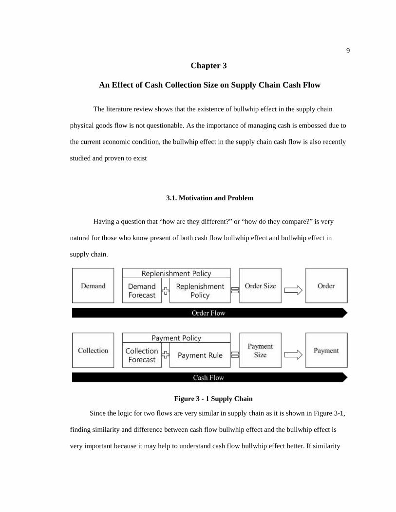
Figure 3 - 1 Supply Chain
Since the logic for two flows are very similar in supply chain as it is shown in Figure 3-1,
finding similarity and difference between cash flow bullwhip effect and the bullwhip effect is
very important because it may help to understand cash flow bullwhip effect better. If similarity

10
can be found, then the cash flow bullwhip effect can be removed or mitigated by way to remove
or mitigate bullwhip effect. The following questions are some possible questions that can be
asked: (1) does impact of lead time on inventory bullwhip effect compare to impact of cash
collection term on cash flow bullwhip effect? (2) does impact of order size on inventory bullwhip
effect compare to impact of cash collection size on cash flow bullwhip effect?
Table 3 - 1 How cash flow bullwhip effect can be compared to bullwhip effect
Inventory Cash
Bullwhip effect on Inventory Bullwhip Effect on Payment?
Lead Time Cash Collection Term?
Batch Order Size Cash Collection Size?
Of the questions that are stated in Table 3 – 1, the question about whether the cash
collection size gives similar impact on cash flow bullwhip effect as the batch order size does to
inventory bullwhip effect, is going to be examined in this chapter.
3.2. Methodology
In order to find out that whether the cash collection size gives similar impact on the cash
flow bullwhip effect as the batch order size, the regression model, whose response variable is
coefficient of variation of payment is built through two full factorial design. Unless changes or
modification are explicitly stated in the thesis, all of assumptions and details are same as
theoretical model introduced in 2011. The decision variables used to build this regression models
are time, cash collection size, lead time, and order size.
Since the experiment is designed to have two levels (Low and High), two levels for each
independent variables are need to be pre-defined: The Low is 60, and the high is 120 for Time.

11
The low is 0.2 and the high is 0.8 for payment ratio of the customer. The low is 2 and the high is
8 for lead time. The low is 40 and high is 160 for order size of the customer as shown Table 3 - 2.
Table 3 - 2 Decision Variables for the DOE
Name Range low high
Time 1 to ∞ 60 120
Collection
Ratio 0 to 1 0.2 0.8
Lead
Time 0 to 10 2 8
Order
Size 0 to 200 40 160
When the variable is a continuous number like this case, it is very difficult to define low
and high value. However, low and high value must be predefined in a way that they are distinct
from each other, yet reasonable. Thus, in order to be reasonable, each variables low and high
value must be chosen within the range of each variable. For variables which are drivers of
bullwhip effect, low is set to be a small number that cannot obviously observe bullwhip effect,
and high is set to be a large number that can obviously observe bullwhip effect. For collection
ratio, 0 for low and 1 for high is too extreme in this case. Therefore, low and high is set to be a
point where they are 0.2 away from minimum or maximum.
In this study, three regression models are going to be built by keeping all variables the
same, but differentiating only the response variables: CV of PAYRetailer, CV of PAYDistributor,
and CV of PAYManufacturer
Since each variable has two levels, only a total of 24or 16 runs is required when the
experiment is built using full factorial design. Furthermore, randomizing the order of the
experiment is unnecessary since the experiment is going to be conducted via computer
simulation, but the order of experiments is randomized anyway. The experiment order and other
details of the design of experiment is summarized in the following Table 3 – 3.
12
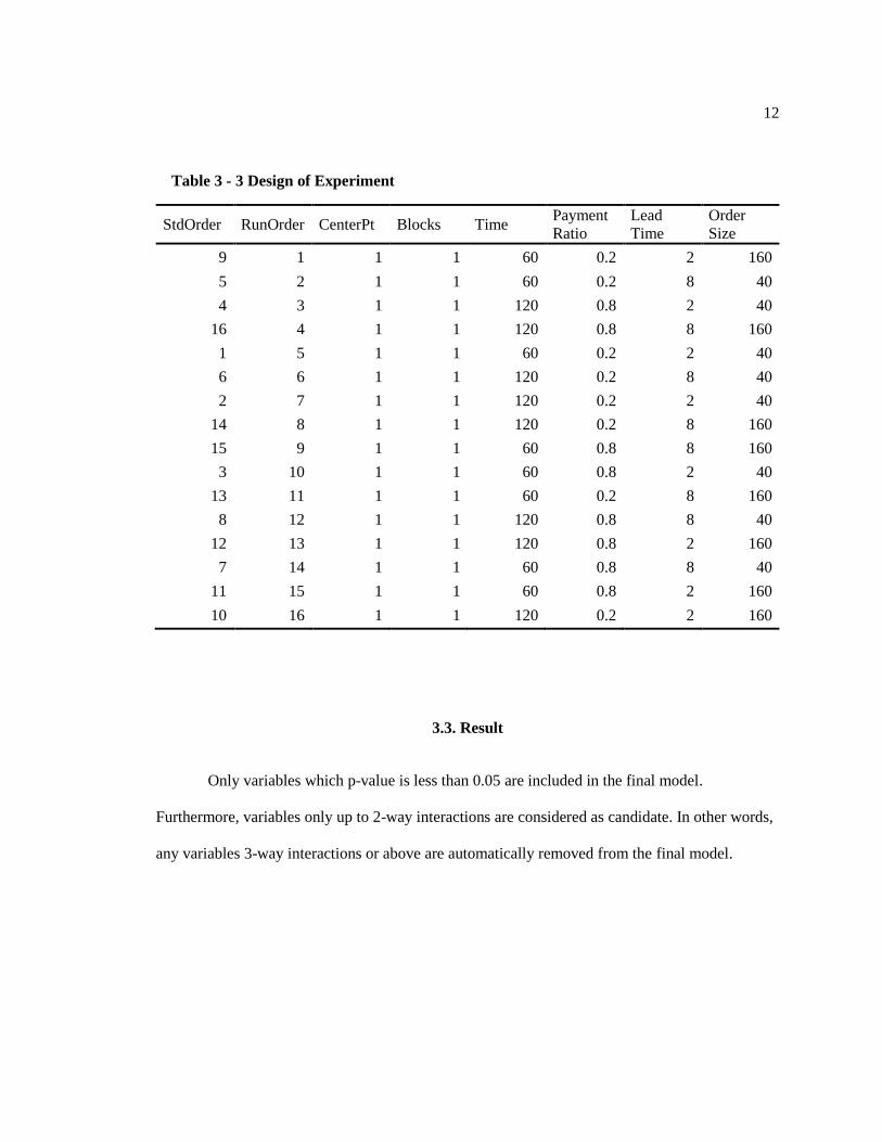
Table 3 - 3 Design of Experiment
StdOrder RunOrder CenterPt Blocks Time Payment
Ratio
Lead
Time
Order
Size
9 1 1 1 60 0.2 2 160
5 2 1 1 60 0.2 8 40
4 3 1 1 120 0.8 2 40
16 4 1 1 120 0.8 8 160
1 5 1 1 60 0.2 2 40
6 6 1 1 120 0.2 8 40
2 7 1 1 120 0.2 2 40
14 8 1 1 120 0.2 8 160
15 9 1 1 60 0.8 8 160
3 10 1 1 60 0.8 2 40
13 11 1 1 60 0.2 8 160
8 12 1 1 120 0.8 8 40
12 13 1 1 120 0.8 2 160
7 14 1 1 60 0.8 8 40
11 15 1 1 60 0.8 2 160
10 16 1 1 120 0.2 2 160
3.3. Result
Only variables which p-value is less than 0.05 are included in the final model.
Furthermore, variables only up to 2-way interactions are considered as candidate. In other words,
any variables 3-way interactions or above are automatically removed from the final model.

13
3.3.1. CV(𝐏𝐚𝐲𝐦𝐞𝐧𝐭𝑹𝒆𝒕𝒂𝒊𝒍𝒆𝒓)
The regression model for the retailer which plays at one level above the customer, is
composed of following six variables: Time, Lead Time, Order Size, Time*Lead Time, Time*
Order size and Lead Time*Order Size. The regression model’s adjusted coefficient determination
is 100%.
Table 3 - 4 Independent Variables included in the Regression Model for Retailer
C.V P PR LT OS T*PR T*LT T*OS PR*LT PR*OS LT*OS
Retailer O O O O O O
Variables included in the final regression model are marked with O
C.V.: Coefficient Variance, T: Time, PR: Payment Ratio
LT: Lead Time, OS: Order Size Estimated Effects and Coefficients for CV_Retailer (coded units)
Term Effect Coef SE Coef T P
Constant 0.6777 0.000217 3126.46 0.000
Time -0.3255 -0.1628 0.000217 -750.95 0.000
Payment_Ratio 0.0000 0.0000 0.000217 0.00 1.000
Lead_Time -0.0242 -0.0121 0.000217 -55.77 0.000
Order_Size -0.0109 -0.0055 0.000217 -25.19 0.000
Time*Payment_Ratio 0.0000 0.0000 0.000217 0.00 1.000
Time*Lead_Time 0.0070 0.0035 0.000217 16.04 0.000
Time*Order_Size 0.0045 0.0023 0.000217 10.42 0.000
Payment_Ratio*Lead_Time -0.0000 -0.0000 0.000217 -0.00 1.000
Payment_Ratio*Order_Size 0.0000 0.0000 0.000217 0.00 1.000
Lead_Time*Order_Size 0.0020 0.0010 0.000217 4.60 0.006
S = 0.000867030 PRESS = 0.0000384892
R-Sq = 100.00% R-Sq(pred) = 99.99% R-Sq(adj) = 100.00%
Analysis of Variance for CV_Retailer (coded units)
Source DF Seq SS Adj SS Adj MS F P
Main Effects 4 0.426738 0.426738 0.106684 141916.25 0.000
Time 1 0.423922 0.423922 0.423922 563919.87 0.000
Payment_Ratio 1 0.000000 0.000000 0.000000 * *
Lead_Time 1 0.002339 0.002339 0.002339 3110.78 0.000
Order_Size 1 0.000477 0.000477 0.000477 634.37 0.000
2-Way Interactions 6 0.000291 0.000291 0.000049 64.53 0.000
Time*Payment_Ratio 1 0.000000 0.000000 0.000000 * *
Time*Lead_Time 1 0.000194 0.000194 0.000194 257.44 0.000
Time*Order_Size 1 0.000082 0.000082 0.000082 108.53 0.000
Payment_Ratio*Lead_Time 1 0.000000 0.000000 0.000000 * *
Payment_Ratio*Order_Size 1 0.000000 0.000000 0.000000 * *
14
Lead_Time*Order_Size 1 0.000016 0.000016 0.000016 21.19 0.006
Residual Error 5 0.000004 0.000004 0.000001
Total 15 0.427032
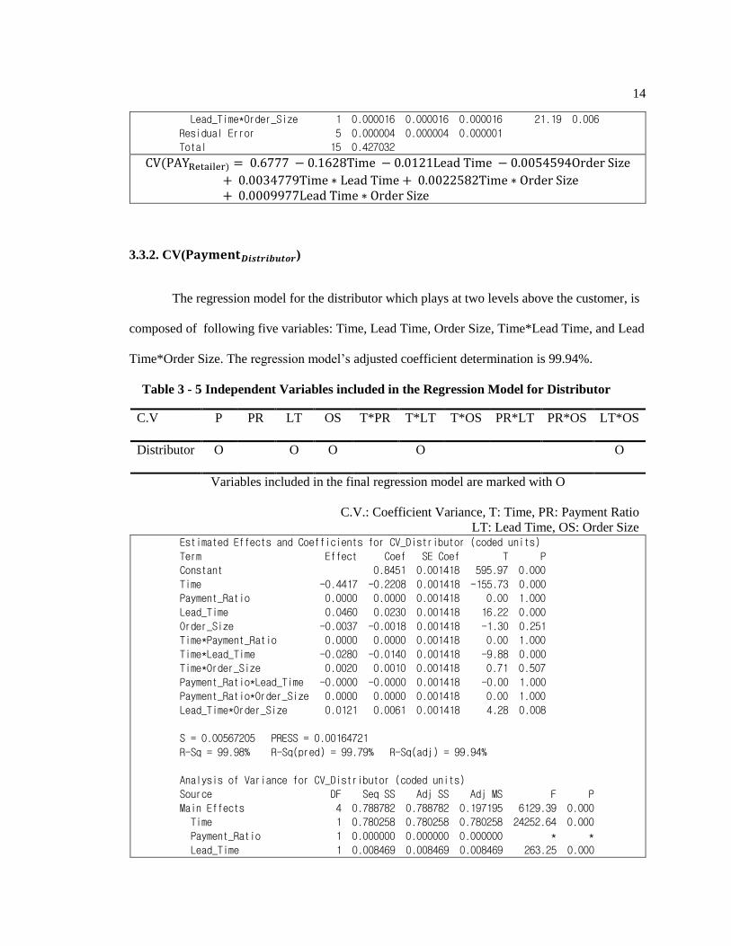
CV(PAYRetailer) = 0.6777 − 0.1628Time − 0.0121Lead Time − 0.0054594Order Size
+ 0.0034779Time ∗ Lead Time + 0.0022582Time ∗ Order Size+ 0.0009977Lead Time ∗ Order Size
3.3.2. CV(𝐏𝐚𝐲𝐦𝐞𝐧𝐭𝑫𝒊𝒔𝒕𝒓𝒊𝒃𝒖𝒕𝒐𝒓)
The regression model for the distributor which plays at two levels above the customer, is
composed of following five variables: Time, Lead Time, Order Size, Time*Lead Time, and Lead
Time*Order Size. The regression model’s adjusted coefficient determination is 99.94%.
Table 3 - 5 Independent Variables included in the Regression Model for Distributor
C.V P PR LT OS T*PR T*LT T*OS PR*LT PR*OS LT*OS
Distributor O O O O O
Variables included in the final regression model are marked with O
C.V.: Coefficient Variance, T: Time, PR: Payment Ratio
LT: Lead Time, OS: Order Size Estimated Effects and Coefficients for CV_Distributor (coded units)
Term Effect Coef SE Coef T P
Constant 0.8451 0.001418 595.97 0.000
Time -0.4417 -0.2208 0.001418 -155.73 0.000
Payment_Ratio 0.0000 0.0000 0.001418 0.00 1.000
Lead_Time 0.0460 0.0230 0.001418 16.22 0.000
Order_Size -0.0037 -0.0018 0.001418 -1.30 0.251
Time*Payment_Ratio 0.0000 0.0000 0.001418 0.00 1.000
Time*Lead_Time -0.0280 -0.0140 0.001418 -9.88 0.000
Time*Order_Size 0.0020 0.0010 0.001418 0.71 0.507
Payment_Ratio*Lead_Time -0.0000 -0.0000 0.001418 -0.00 1.000
Payment_Ratio*Order_Size 0.0000 0.0000 0.001418 0.00 1.000
Lead_Time*Order_Size 0.0121 0.0061 0.001418 4.28 0.008
S = 0.00567205 PRESS = 0.00164721
R-Sq = 99.98% R-Sq(pred) = 99.79% R-Sq(adj) = 99.94%
Analysis of Variance for CV_Distributor (coded units)
Source DF Seq SS Adj SS Adj MS F P
Main Effects 4 0.788782 0.788782 0.197195 6129.39 0.000
Time 1 0.780258 0.780258 0.780258 24252.64 0.000
Payment_Ratio 1 0.000000 0.000000 0.000000 * *
Lead_Time 1 0.008469 0.008469 0.008469 263.25 0.000

15
Order_Size 1 0.000054 0.000054 0.000054 1.68 0.251
2-Way Interactions 6 0.003748 0.003748 0.000625 19.42 0.003
Time*Payment_Ratio 1 0.000000 0.000000 0.000000 * *
Time*Lead_Time 1 0.003143 0.003143 0.003143 97.68 0.000
Time*Order_Size 1 0.000016 0.000016 0.000016 0.51 0.507
Payment_Ratio*Lead_Time 1 0.000000 0.000000 0.000000 * *
Payment_Ratio*Order_Size 1 0.000000 0.000000 0.000000 * *
Lead_Time*Order_Size 1 0.000589 0.000589 0.000589 18.30 0.008
Residual Error 5 0.000161 0.000161 0.000032
Total 15 0.792690
CV(PAYDistributor)= 0.845099 − 0.220831Time + 0.023007Lead Time − 0.0014015Time∗ Lead Time + 0.006066Lead Time ∗ Order Size
3.3.3. CV(𝐏𝐚𝐲𝐦𝐞𝐧𝐭𝒎𝒂𝒏𝒖𝒇𝒂𝒄𝒕𝒖𝒓𝒆𝒓)
The regression model for the manufacturer which plays at three levels above the
customer, is composed of following five variables: Time, Lead Time, Order Size, Time*Lead
Time, and Lead Time*Order Size. The adjusted coefficient determination is 99.04%.
Table 3 - 6 Independent Variables included in the Regression Model for Manufacturer
C.V P PR LT OS T*PR T*LT T*OS PR*LT PR*OS LT*OS
MFG O O O O O
Variables included in the final regression model are marked with O
C.V.: Coefficient Variance, T: Time, PR: Payment Ratio
LT: Lead Time, OS: Order Size Estimated Effects and Coefficients for CV_MFG (coded units)
Term Effect Coef SE Coef T P
Constant 1.3919 0.01912 72.79 0.000
Time -1.1489 -0.5744 0.01912 -30.04 0.000
Payment_Ratio 0.0000 0.0000 0.01912 0.00 1.000
Lead_Time 0.8147 0.4074 0.01912 21.30 0.000
Order_Size 0.0912 0.0456 0.01912 2.39 0.063
Time*Payment_Ratio -0.0000 -0.0000 0.01912 -0.00 1.000
Time*Lead_Time -0.6236 -0.3118 0.01912 -16.31 0.000
Time*Order_Size -0.0793 -0.0396 0.01912 -2.07 0.093
Payment_Ratio*Lead_Time -0.0000 -0.0000 0.01912 -0.00 1.000
Payment_Ratio*Order_Size 0.0000 0.0000 0.01912 0.00 1.000
Lead_Time*Order_Size 0.1021 0.0511 0.01912 2.67 0.044
S = 0.0764875 PRESS = 0.299538
R-Sq = 99.70% R-Sq(pred) = 96.89% R-Sq(adj) = 99.09%

16
Analysis of Variance for CV_MFG (coded units)
Source DF Seq SS Adj SS Adj MS F P
Main Effects 4 7.96835 7.96835 1.99209 340.51 0.000
Time 1 5.27981 5.27981 5.27981 902.48 0.000
Payment_Ratio 1 0.00000 0.00000 0.00000 * *
Lead_Time 1 2.65523 2.65523 2.65523 453.86 0.000
Order_Size 1 0.03330 0.03330 0.03330 5.69 0.063
2-Way Interactions 6 1.62257 1.62257 0.27043 46.22 0.000
Time*Payment_Ratio 1 0.00000 0.00000 0.00000 * *
Time*Lead_Time 1 1.55571 1.55571 1.55571 265.92 0.000
Time*Order_Size 1 0.02515 0.02515 0.02515 4.30 0.093
Payment_Ratio*Lead_Time 1 0.00000 0.00000 0.00000 * *
Payment_Ratio*Order_Size 1 0.00000 0.00000 0.00000 * *
Lead_Time*Order_Size 1 0.04171 0.04171 0.04171 7.13 0.044
Residual Error 5 0.02925 0.02925 0.00585
CV(PAYMfg) = 1.3919 − 0.5744Time + 0.4074Lead Time + 0.0456Order Size −
0.3118Time ∗ Lead Time + 0.0511Lead Time ∗ Order Size
3.3.4. CV(𝐏𝐚𝐲𝐦𝐞𝐧𝐭𝑺𝒖𝒑𝒑𝒍𝒊𝒆𝒓)
The regression model for the supplier which plays at four levels above the customer, is
composed of following five variables: Time, Lead Time, Order Size, Time*Lead Time, and Lead
Time*Order Size. The regression model’s adjusted coefficient determination is 99.98%.
Table 3 - 7 Independent Variables included in the Regression Model for Supplier
C.V P PR LT OS T*PR T*LT T*OS PR*LT PR*OS LT*OS
Supplier O O O O O
Variables included in the final regression model are marked with O
C.V.: Coefficient Variance, T: Time, PR: Payment Ratio
LT: Lead Time, OS: Order Size Estimated Effects and Coefficients for CV_Supplier (coded units)
Term Effect Coef SE Coef T P
Constant 1.9236 0.003773 509.79 0.000
Time -0.9867 -0.4934 0.003773 -130.75 0.000
Payment_Ratio 0.0000 0.0000 0.003773 0.00 1.000
Lead_Time 1.5201 0.7601 0.003773 201.43 0.000
Order_Size 0.2206 0.1103 0.003773 29.24 0.000
Time*Payment_Ratio -0.0000 -0.0000 0.003773 -0.00 1.000
Time*Lead_Time -0.3243 -0.1621 0.003773 -42.97 0.000
Time*Order_Size -0.0121 -0.0060 0.003773 -1.60 0.170
Payment_Ratio*Lead_Time -0.0000 -0.0000 0.003773 -0.00 1.000

17
Payment_Ratio*Order_Size 0.0000 0.0000 0.003773 0.00 1.000
Lead_Time*Order_Size 0.2303 0.1152 0.003773 30.52 0.000
S = 0.0150935 PRESS = 0.0116641
R-Sq = 99.99% R-Sq(pred) = 99.92% R-Sq(adj) = 99.98%
Analysis of Variance for CV_Supplier (coded units)
Source DF Seq SS Adj SS Adj MS F P
Main Effects 4 13.3323 13.3323 3.33308 14630.70 0.000
Time 1 3.8947 3.8947 3.89467 17095.80 0.000
Payment_Ratio 1 0.0000 0.0000 0.00000 * *
Lead_Time 1 9.2429 9.2429 9.24292 40572.19 0.000
Order_Size 1 0.1947 0.1947 0.19474 854.80 0.000
2-Way Interactions 6 0.6334 0.6334 0.10557 463.38 0.000
Time*Payment_Ratio 1 0.0000 0.0000 0.00000 * *
Time*Lead_Time 1 0.4206 0.4206 0.42062 1846.33 0.000
Time*Order_Size 1 0.0006 0.0006 0.00058 2.57 0.170
Payment_Ratio*Lead_Time 1 0.0000 0.0000 0.00000 * *
Payment_Ratio*Order_Size 1 0.0000 0.0000 0.00000 * *
Lead_Time*Order_Size 1 0.2122 0.2122 0.21219 931.41 0.000
Residual Error 5 0.0011 0.0011 0.00023
9Total 15 13.9669
CV(PAYSupplier)
= 1.9236 − 0.4934Time + 0.7601Lead Time + 0.1103Order Size− 0.3118Time ∗ Lead Time + 0.1152Lead Time ∗ Order Size
3.4. Conclusive Remarks
Prior to discussing the observation of this experiment, it is important to mention the
difference between the Liu’s observation and this thesis’ observation. Liu’s experiment and this
experiment differ in the focus of experiment; In 2011, Liu also built a regression using DOE.
However, Liu’s model is more focused on identifying the effect of the moving term used in
demand forecast and payment forecast, while the object of this experiment is more focused on
identifying the effect of the cash collection size. As a result, the variables used to build the model
is also different. In Liu’s model, the independent variable candidates are: Payment Forecast,
Credit Term, Demand Forecast and Lead Time. While this model’s independent variable
candidates are: Time, Cash Collection Ratio, Lead Time and Order Size.
18
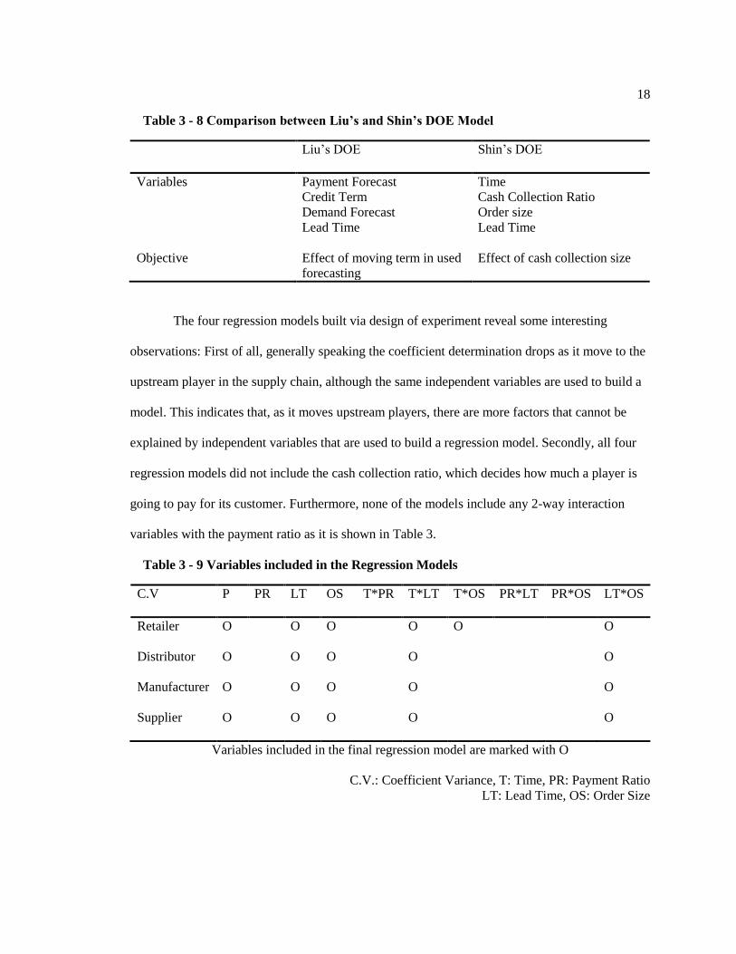
Table 3 - 8 Comparison between Liu’s and Shin’s DOE Model
Liu’s DOE Shin’s DOE
Variables Payment Forecast
Credit Term
Demand Forecast
Lead Time
Time
Cash Collection Ratio
Order size
Lead Time
Objective
Effect of moving term in used
forecasting
Effect of cash collection size
The four regression models built via design of experiment reveal some interesting
observations: First of all, generally speaking the coefficient determination drops as it move to the
upstream player in the supply chain, although the same independent variables are used to build a
model. This indicates that, as it moves upstream players, there are more factors that cannot be
explained by independent variables that are used to build a regression model. Secondly, all four
regression models did not include the cash collection ratio, which decides how much a player is
going to pay for its customer. Furthermore, none of the models include any 2-way interaction
variables with the payment ratio as it is shown in Table 3.
Table 3 - 9 Variables included in the Regression Models
C.V P PR LT OS T*PR T*LT T*OS PR*LT PR*OS LT*OS
Retailer O O O O O O
Distributor O O O O O
Manufacturer O O O O O
Supplier O O O O O
Variables included in the final regression model are marked with O
C.V.: Coefficient Variance, T: Time, PR: Payment Ratio
LT: Lead Time, OS: Order Size
19
This observation indicates that the cv(Payment) is not depended on the size of cash collection. In
other words, the size of cash collection either doesn’t give any effect or gives to insignificant
effect to the cash flow bullwhip effect.
In sum, from the observations of this experiment, the following points can be concluded:
first of all, variables, such as: lead time, order size and time are also identified as variables that
have some impact on cash flow bullwhip effect. According to the regression models, the average
of approximately 98% of cv(payment) variation can be explained with variables mentioned
above. Secondly, the size of cash collection is not included in a regression model. In other words,
whether the customer pays in full or a small fraction of what he or she owes, it really doesn’t
matter to the cash flow bullwhip effect. The cash flow bullwhip effect either is not affected or is
marginally affected by the size of cash collection.

20
Chapter 4
An effect of Cash Collection Ratio Variation on Supply Chain Cash Flow
4.1. Motivation and Problem
From the result of the previous chapter, the size of cash collection does not affect the
cash flow bullwhip effect. However, as it is mentioned in the introduction, many of the SMEs
suffered because their customers did not pay what they owed in times of financial crisis as the
economic conditions change. In other words, this fact illustrates that cash collection ratio is
somehow related to cash flow in supply chain.
If the size of cash collection ratio is irrelevant to the cash flow bullwhip effect, than there
must be a hidden relationship between them. In the end, this leads to another problem that needs
to be answered. As it is shown in the chapter 3, if the size of cash collection is irrelevant to the
cash flow bullwhip effect, how or in what way does cash collection ratio affect the cash flow
bullwhip?
4.2. Methodology
In this chapter, in order to find the hidden relationship between cash flow bullwhip and
the cash collection ratio, the components which impact the cash flow bullwhip effect are
analytically derived from cv(payment). As the next step, the way in which the cash collection
ratio affects cv(Payment) is analytically identified. After that, the cv(Payment) is calculated for
every players in the supply chain using equation derived analytically. In the end, the analytic
model’s result is compared to the result of the simulation model for the validation purpose.

21
4.3. Derivation and Result
The cash flow bullwhip effect is measured by cv(Payment). The coefficient of variation is
the ratio of standard deviation over the mean, also known as normalized standard deviation. The
reason normalized standard deviation is used in the model is because the price for different
members are different. Thus, in order to compare variance of each player, the normalized
standard deviation is required. The Payment is defined as following:
𝑃𝐴𝑌𝑡+1 = �̂�𝑡+1 ∗ 𝑂𝑡−1
Therefore, payment can also be expressed as following:
𝑃𝐴𝑌𝑡 = �̂�𝑡 ∗ 𝑂𝑡−2 (1)
The Payment is composed of forecast of collection ratio and the order made. In addition,
the forecasting is made based on exponential smoothing. Therefore, forecast of collection ratio
can be expressed as following:
�̂�𝑡+1 = 𝛼𝛽𝑡 + (1 − 𝛼)�̂�𝑡
�̂�𝑡 = 𝛼𝛽𝑡−1 + (1 − 𝛼)�̂�𝑡−1
(2)
in which, 𝛽𝑡 is collection ratio at time t which is expressed as shown below:
𝛽𝑡 = {
𝑐𝑜𝑙𝑙𝑒𝑐𝑡𝑖𝑜𝑛 𝑓𝑜𝑟 𝑠𝑎𝑙𝑒 𝑎𝑡 (𝑡 − 2)
𝑠𝑎𝑙𝑒𝑠 𝑎𝑡 (𝑡 − 2), |𝑖𝑓 𝑠𝑎𝑙𝑒𝑠 𝑎𝑡 (𝑡 − 2) ≠ 0
0 , |𝑖𝑓 𝑠𝑎𝑙𝑒𝑠 𝑎𝑡 (𝑡 − 2) = 0
(3)
Using equation (1) and (3), the relationship between the collection ratio of player j and
the forecast collection ratio of player j-1 can be derived as following:
𝜷𝒋𝒕 =
𝒄𝒐𝒍𝒍𝒆𝒄𝒕𝒊𝒐𝒏 𝒇𝒐𝒓 𝒔𝒂𝒍𝒆 𝒂𝒕 (𝒕 − 𝟐)
𝒔𝒂𝒍𝒆𝒔 𝒂𝒕 (𝒕 − 𝟐)=
𝑷𝑨𝒀𝒋−𝟏𝒕
𝑶𝒋−𝟏𝒕−𝟐
=�̂�𝒋−𝟏
𝒕 ∗ 𝑶𝒋−𝟏𝒕−𝟐
𝑶𝒋−𝟏𝒕−𝟐
= �̂�𝒋−𝟏𝒕
This derivation shows that the collection ratio of player j is dependent on the previous
player’s forecast collection ratio. In sum, every players’ collection ratio in the supply chain is
22
dependent on the payment of the last player of the supply chain, which is also known as the
customer of the supply chain.
In general, exponential smoothing forecast can be defined as following:
𝑆𝑡 = 𝛼𝑋𝑡−1 + (1 − 𝛼)𝑆𝑡−1
And if we expand the above equation. We get:
𝑆𝑡 = 𝛼[𝑋𝑡−1 + (1 − 𝛼)𝑋𝑡−2 + (1 − 𝛼)2𝑋𝑡−3 + ⋯ + (1 − 𝛼)𝑡−1𝑋0] + (1 − 𝛼)𝑡𝑆0
𝑆𝑡 = ∑ 𝛼(1 − 𝛼)𝑖𝑋𝑡−𝑖−1
𝑡−1
𝑖=0
(4)
Furthermore, writing equation (4) in terms of collection ratio (𝛽𝑗𝑡) and forecast collection
ratio (�̂�𝑗𝑡), can be express as following:
�̂�𝑡 = ∑ 𝛼(1 − 𝛼)𝑖𝛽𝑡−𝑖−1
𝑡−1
𝑖=0
(5)
By the definition of cv(Payment),
cv(𝑃𝐴𝑌𝑗) =𝑠𝑡𝑑(𝑃𝐴𝑌𝑗)
𝑚𝑒𝑎𝑛(𝑃𝐴𝑌𝑗)
(6)
cv(𝑃𝐴𝑌𝑗) can be also expressed as following:

23
cv(𝑃𝐴𝑌𝑗) =𝑠𝑡𝑑(𝑃𝐴𝑌𝑗)
𝑚𝑒𝑎𝑛(𝑃𝐴𝑌𝑗)=
𝑠𝑡𝑑(�̂�𝑗 ∗ 𝑃𝑟𝑗+1 ∗ 𝑂𝑗)
𝐸(�̂�𝑗 ∗ 𝑃𝑟𝑗+1 ∗ 𝑂𝑗)=
𝑃𝑟𝑗+1 ∗ 𝑠𝑡𝑑(�̂�𝑗 ∗ 𝑂𝑗)
𝑃𝑟𝑗+1 ∗ 𝐸(�̂�𝑗)𝐸(𝑂𝑗)
= √𝑉𝑎𝑟(�̂�𝑗 ∗ 𝑂𝑗)
(𝐸(�̂�𝑗)𝐸(𝑂𝑗))2
= √𝐸(�̂�𝑗)
2𝑉𝑎𝑟(𝑂𝑗) + 𝐸(𝑂𝑗)
2𝑉𝑎𝑟(�̂�𝑗) + 𝑉𝑎𝑟(�̂�𝑗)𝑉𝑎𝑟(𝑂𝑗)
(𝐸(�̂�𝑗)𝐸(𝑂𝑗))2
= √𝑉𝑎𝑟(𝑂𝑗)
𝐸(𝑂𝑗)2 +
𝑉𝑎𝑟(�̂�𝑗)
𝐸(�̂�𝑗)2 +
𝑉𝑎𝑟(�̂�𝑗)
𝐸(�̂�𝑗)2 ∗
𝑉𝑎𝑟(𝑂𝑗)
𝐸(𝑂𝑗)2
= cv(𝑂𝑗) + cv(�̂�𝑗) + cv(�̂�𝑗) ∗ 𝑐𝑣(𝑂𝑗)
= 𝐜𝐯(𝑶𝒋) + (𝟏 + 𝐜𝐯(𝑶𝒋)) 𝐜𝐯(�̂�𝒋)
(7)
Equation 7, derived from the definition of cv(Payment), indicates that cv(Payment) is
composed of cv(𝑂𝑗), cv(�̂�𝑗)and interaction of these two. Furthermore, since the �̂�𝑗 is derived
from the exponential smoothing method, cv(Payment) can also be expressed as following:
cv(𝑃𝐴𝑌𝑗) = cv(𝑂𝑗) + (1 + cv(𝑂𝑗)) cv(�̂�𝑗) = 𝑐𝑣(𝑂𝑗) + (1 + cv(𝑂𝑗)) ∗ √𝑉𝑎𝑟(�̂�𝑗)
𝐸(�̂�𝑗)2
= 𝒄𝒗(𝑶𝒋) + (𝟏 + 𝐜𝐯(𝑶𝒋)) ∗ √𝑽𝒂𝒓(∑ 𝜶(𝟏 − 𝜶)𝒊𝜷𝒕−𝒊−𝟏
𝒕−𝟏𝒊=𝟎 )
𝑬(�̂�𝒋)𝟐
(8)
As it is mentioned above, the equation (7) suggests that cv(Payment) is subjected by two
coefficients of variation: order made and collection ratio. Since this thesis is focused on the effect
of cash collection, instead of identifying the impact of all components of cv(Payment), the rest of
this section is focused on studying the effect of C.V(�̂�𝑗) to the cash flow bullwhip effect.

24
4.3.1. Normal Distribution and Exponential Distribution
Let’s assume that collection ratio follows normal distribution [β~𝑁(𝜇, 𝜎2)] and it is
independent. Then the equation (8) can be expressed as following:
cv(𝑃𝐴𝑌𝑗) = 𝑐𝑣(𝑂𝑗) + (1 + 𝑐𝑣(𝑂𝑗)) ∗ √𝑉𝑎𝑟(∑ 𝛼(1 − 𝛼)𝑖𝛽𝑡−𝑖−1
𝑡−1𝑖=0 )
𝐸(∑ 𝛼(1 − 𝛼)𝑖𝛽𝑡−𝑖−1𝑡−1𝑖=0 )
2
= 𝑐𝑣(𝑂𝑗) + (1 + 𝑐𝑣(𝑂𝑗)) ∗ √∑ (𝛼(1 − 𝛼)𝑖)2𝑉𝑎𝑟(𝛽𝑡−𝑖−1)𝑡−1
𝑖=0
(∑ 𝛼(1 − 𝛼)𝑖𝐸(𝛽𝑡−𝑖−1)𝑡−1𝑖=0 )
2
= 𝑐𝑣(𝑂𝑗) + (1 + 𝑐𝑣(𝑂𝑗)) ∗ √∑ (𝛼(1 − 𝛼)𝑖)2𝜎𝛽𝑡−𝑖−1
2𝑡−1𝑖=0
(∑ 𝛼(1 − 𝛼)𝑖𝜇𝛽𝑡−𝑖−1
𝑡−1𝑖=0 )
2
= 𝑐𝑣(𝑂𝑗) + (1 + 𝑐𝑣(𝑂𝑗)) ∗∑ 𝛼(1 − 𝛼)𝑖𝜎𝛽𝑡−𝑖−1
𝑡−1𝑖=0
∑ 𝛼(1 − 𝛼)𝑖𝜇𝛽𝑡−𝑖−1
𝑡−1𝑖=0
= 𝒄𝒗(𝑶𝒋) + (𝟏 + 𝒄𝒗(𝑶𝒋)) ∗∑ 𝜶(𝟏 − 𝜶)𝒊𝝈𝜷𝒕−𝒊−𝟏
𝒕−𝟏𝒊=𝟎
𝝁𝜷
(9)
Instead of assuming normal distribution, let’s assume that collection ratio follows
exponential distribution [β~𝑒𝑥𝑝 (1
𝜆)] and is independent. Then, the equation (8) can be expressed
as following:

25
cv(𝑃𝐴𝑌𝑗) = 𝑐𝑣(𝑂𝑗) + (1 + 𝑐𝑣(𝑂𝑗)) cv(�̂�𝑗)
= 𝑐𝑣(𝑂𝑗) + (1 + 𝑐𝑣(𝑂𝑗)) ∗ √𝑉𝑎𝑟(∑ 𝛼(1 − 𝛼)𝑖𝛽𝑡−𝑖−1
𝑡−1𝑖=0 )
𝐸(∑ 𝛼(1 − 𝛼)𝑖𝛽𝑡−𝑖−1𝑡−1𝑖=0 )
2
= 𝑐𝑣(𝑂𝑗) + (1 + 𝑐𝑣(𝑂𝑗)) ∗ √∑ (𝛼(1 − 𝛼)𝑖)2𝑉𝑎𝑟(𝛽𝑡−𝑖−1)𝑡−1
𝑖=0
(∑ 𝛼(1 − 𝛼)𝑖𝐸(𝛽𝑡−𝑖−1)𝑡−1𝑖=0 )
2
= 𝑐𝑣(𝑂𝑗) + (1 + 𝑐𝑣(𝑂𝑗)) ∗ √
∑ (𝛼(1 − 𝛼)𝑖)2𝑡−1𝑖=0
1𝜆𝛽𝑡−𝑖−1
2
(∑ 𝛼(1 − 𝛼)𝑖 1𝜆𝛽𝑡−𝑖−1
𝑡−1𝑖=0 )
2
= 𝑐𝑣(𝑂𝑗) + (1 + 𝑐𝑣(𝑂𝑗)) ∗
∑ 𝛼(1 − 𝛼)𝑖 1𝜆𝛽𝑡−𝑖−1
𝑡−1𝑖=0
∑ 𝛼(1 − 𝛼)𝑖 1𝜆𝛽𝑡−𝑖−1
𝑡−1𝑖=0
= 𝒄𝒗(𝑶𝒋) + (𝟏 + 𝒄𝒗(𝑶𝒋)) ∗ 𝟏
(10)
The equation (9) and equation (10) is similar in which both equations start with 𝑐𝑣(𝑂𝑗) +
(1 + 𝑐𝑣(𝑂𝑗)). However, two equations differ in the last component of the equations because
different distribution is assumed. Thus, in order to see the impact of the difference in the
distribution of the cash collection ratio, the cv(Payment) is calculated when both distributions
have same mean and variance but when they have different distributions. The mean is set to be
0.45 because the replications of simulation model’s cash collection ratio is approximately 0.45
and variance is set to be 0.2025 for both distribution because the variance of exponential
distribution is pre-defined as 𝐸2 by the definition. . Given that β~𝑁(0.45, 0.2025) or
β~𝑒𝑥𝑝 (1
𝜆= 0.45) and 𝑐𝑣(𝑂𝑗) is as shown in Table 4 – 1, cv(Payment) for each player can be
calculated as following:

26
Table 4 - 1 Coefficient of variation of Oj
Coefficient of variation of 𝑂𝑗
Customer Retailer Distributor MFG Supplier
0.4853 0.5929 0.8366 1.2917 1.9112
Result of the Normal Distribution
cv(𝑃𝐴𝑌𝑗=1) = 𝑐𝑣(𝑂𝑗=1) + (1 + 𝑐𝑣(𝑂𝑗=1)) ∗∑ 𝛼(1 − 𝛼)𝑖𝜎𝛽𝑡−𝑖−1
𝑡−1𝑖=0
𝜇𝛽
= 0.49 + (1 + 0.49) ∗0.1034
0.45= 0.832369
cv(𝑃𝐴𝑌𝑗=2) = 𝑐𝑣(𝑂𝑗=2) + (1 + 𝑐𝑣(𝑂𝑗=2)) ∗∑ 𝛼(1 − 𝛼)𝑖𝜎𝛽𝑡−𝑖−1
𝑡−1𝑖=0
𝜇𝛽
= 0.5929 + (1 + 0.5929) ∗0.1034
0.45= 0.958913
cv(𝑃𝐴𝑌𝑗=3) = 𝑐𝑣(𝑂𝑗=3) + (1 + 𝑐𝑣(𝑂𝑗=3)) ∗∑ 𝛼(1 − 𝛼)𝑖𝜎𝛽𝑡−𝑖−1
𝑡−1𝑖=0
𝜇𝛽
= 0.8366 + (1 + 0.8366) ∗0.1034
0.45= 1.25861
cv(𝑃𝐴𝑌𝑗=4) = 𝑐𝑣(𝑂𝑗=4) + (1 + 𝑐𝑣(𝑂𝑗=4)) ∗∑ 𝛼(1 − 𝛼)𝑖𝜎𝛽𝑡−𝑖−1
𝑡−1𝑖=0
𝜇𝛽
= 1.2917 + (1 + 1.2917) ∗0.1034
0.45= 1.818282
cv(𝑃𝐴𝑌𝑗=5) = 𝑐𝑣(𝑂𝑗=5) + (1 + 𝑐𝑣(𝑂𝑗=5)) ∗∑ 𝛼(1 − 𝛼)𝑖𝜎𝛽𝑡−𝑖−1
𝑡−1𝑖=0
𝜇𝛽
= 1.9112 + (1 + 1.9112) ∗0.1034
0.45= 2.580129

27
Figure 4 - 1 Comparison between Simulation and Analytic (Normal) Result
Result of the Exponential Distribution
cv(𝑃𝐴𝑌𝑗=1) = 𝑐𝑣(𝑂𝑗=1) + (1 + 𝑐𝑣(𝑂𝑗=1)) ∗ 1 = 0.4853 + (1 + 0.4853) ∗ 1 = 1.9706
cv(𝑃𝐴𝑌𝑗=2) = 𝑐𝑣(𝑂𝑗=2) + (1 + 𝑐𝑣(𝑂𝑗=2)) ∗ 1 = 0.5929 + (1 + 0.5929) ∗ 1 = 2.1858
cv(𝑃𝐴𝑌𝑗=3) = 𝑐𝑣(𝑂𝑗=3) + (1 + 𝑐𝑣(𝑂𝑗=3)) ∗ 1 = 0.8366 + (1 + 0.8366) ∗ 1 = 2.6732
cv(𝑃𝐴𝑌𝑗=4) = 𝑐𝑣(𝑂𝑗=4) + (1 + 𝑐𝑣(𝑂𝑗=4)) ∗ 1 = 1.2917 + (1 + 1.2917) ∗ 1 = 3.5834
cv(𝑃𝐴𝑌𝑗=5) = 𝑐𝑣(𝑂𝑗=5) + (1 + 𝑐𝑣(𝑂𝑗=5)) ∗ 1 = 1.9112 + (1 + 1.9112) ∗ 1 = 4.8224
Customer Retailer Distributor MFG Supplier
Simulation Model 0.7869 0.6234 0.8871 1.3874 2.1740
Analytic Model 0.8324 0.9589 1.2586 1.8183 2.5801
0.0000
0.5000
1.0000
1.5000
2.0000
2.5000
3.0000
Simulation VS Analyic (Normal)
28
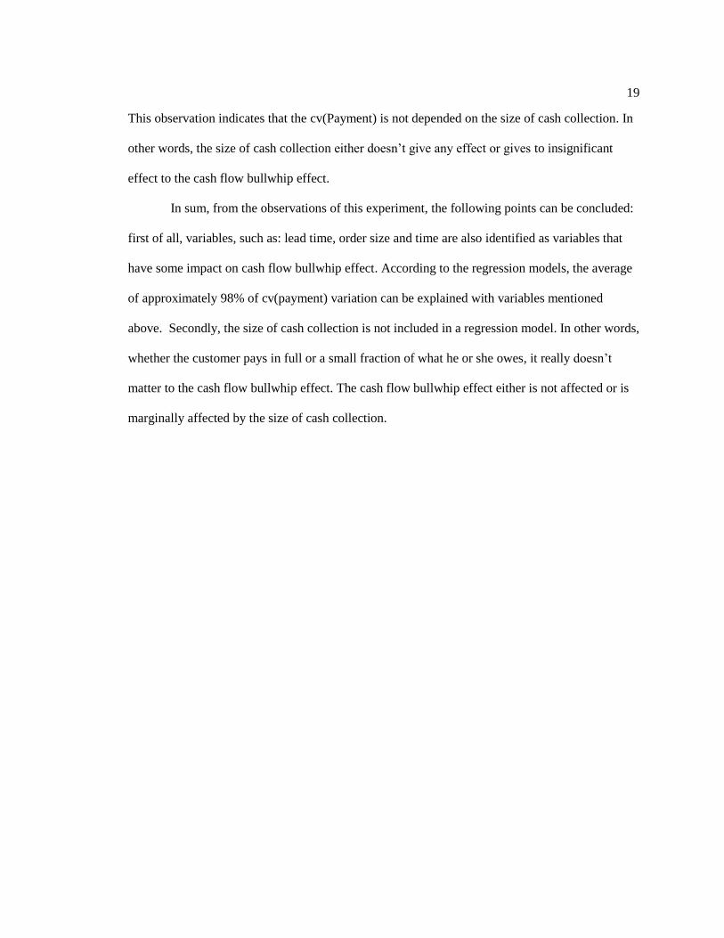
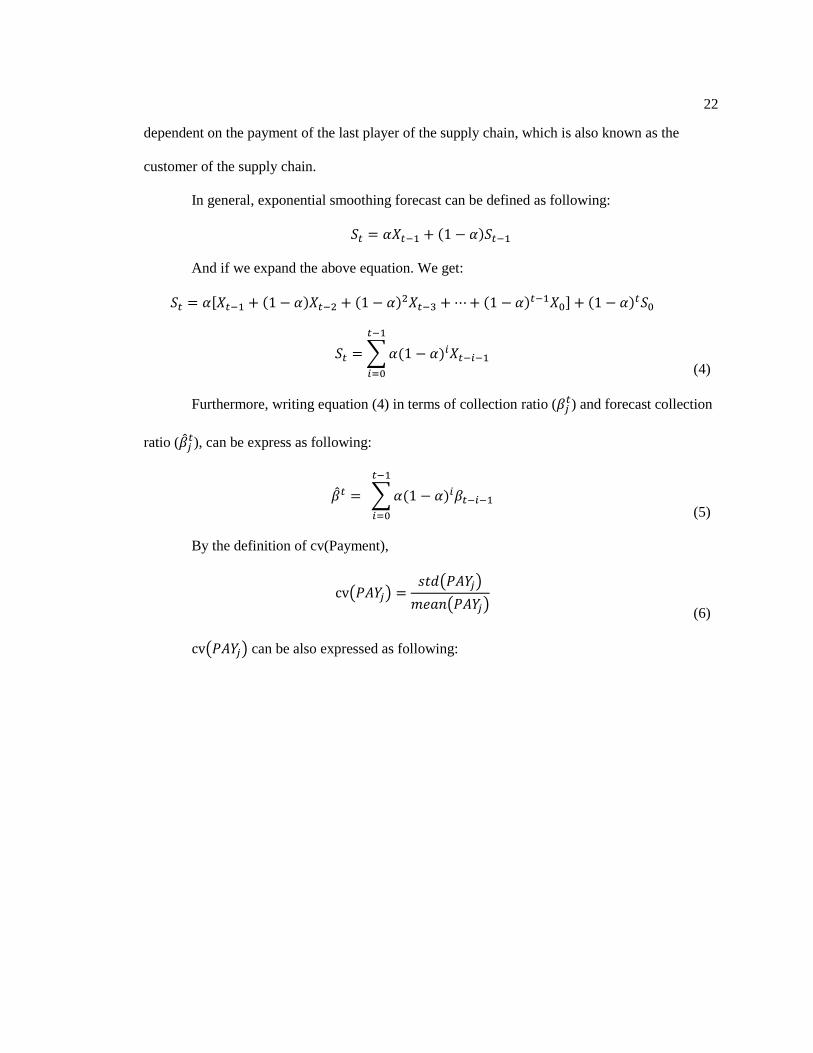
Figure 4 - 2 Comparison between Simulation and Analytic (Exponential) Result
Although all other components of cv(Payment) remain the same, the result of the two
analytic models is significantly different as this is shown in Figure 4 – 3. This difference comes
from the difference in the distribution of the cash collection ratio.
Figure 4 - 3 Comparison of C.V.
Customer Retailer Distributor MFG Supplier
Simulation Model 0.7869 0.6234 0.8871 1.3874 2.1740
Analytic Model 1.9706 2.1858 2.6732 3.5834 4.8224
0.0000
1.0000
2.0000
3.0000
4.0000
5.0000
6.0000
Simulation vs Analytic (Exponential)
Customer Retailer Distributor MFG Supplier
Simulation Model 0.7869 0.6234 0.8871 1.3874 2.1740
Normal 0.8324 0.9589 1.2586 1.8183 2.5801
Exponential 1.9706 2.1858 2.6732 3.5834 4.8224
0.0000
1.0000
2.0000
3.0000
4.0000
5.0000
6.0000
Comparison of C.V.

29
4.3.3. Family of Normal Distribution
As it shown in the Figure 4- 4, there are thousands of normal distributions with the same
mean. In the previous section, the result of the normal model is similar to the result of the
simulation model, but significantly different from the result of the exponential model although
assumed distribution of the cash collection ratio is different.
One of possible reasons is due to the difference in variance. In other words, the result of
the normal model may differ depending on the variance of the distribution.
Figure 4 - 4 Family of Normal Distribution
Thus in this section, the changes of C.V. Payment are observed when the variance of
normal distribution changes. By doing so, the effect of different variance size can be identified. A
family of normal distribution with mean of 0.45 is tested: N(0.45, 0.1), N(0.45, 0.2), N(0.45, 0.5),
N(0.45, 1), N(0.45, 3), N(0.45, 5), N(0.45, 7), N(0.45, 9),and N(0.45, 10).
The C.V. Payment for each player in the supply chain is calculated using equation (9) and
the result of calculation is summarized. The summary is shown in Table 4 – 2.

30
Table 4 - 2 Family of Normal Distribution with Mean of 0.45
v(0.1) v(0.2) v(0.5) v(1) v(3) v(5) v(7) v(9) v(10)
Customer 0.5 0.52 0.57 0.66 1.01 1.35 1.7 2.05 2.22
Retailer 0.61 0.63 0.68 0.78 1.15 1.52 1.9 2.27 2.45
Distributor 0.86 0.88 0.94 1.05 1.48 1.91 2.34 2.77 2.98
MFG 1.32 1.35 1.42 1.56 2.1 2.63 3.17 3.71 3.97
Supplier 1.94 1.98 2.08 2.25 2.93 3.61 4.29 4.98 5.31
As Table 4 – 2 and Figure 4 – 5 show, the C.V. Payment of each player in the supply
chain increases as the variance of the normal distribution increases. In addition, when the size of
variance is big enough, cv(Payment) of each player, which cash collection follows normal
distribution, is similar to cv(Payment) which cash collection follows exponential distribution.
This is shown in the Figure 4 – 5.
Figure 4 - 5 Comparison between Family of Normal Dis. and Exponential Dis.
In addition to size of variance, in case of the normal distribution, the smoothing
parameter of the forecast method cannot be ignored. On the other hand, in case of the exponential
distribution, the smoothing parameter of the forecast method can be ignored; it is because as it is
0.00
1.00
2.00
3.00
4.00
5.00
6.00
Customer Retailer Distributor MFG Supplier
Family of Normal Distribution (μ=0.45) vs Exp
v(0.1) v(0.2) v(0.5) v(1) v(3) v(4) Exp
31
shown in the equation (10), in the case of exponential distribution, the smoothing parameter is
canceled out in the final equation.
4.4. Conclusive Remarks
In this chapter, the effect of cash collection ratio’s variance on Cash bullwhip is studied.
By analytically deriving the components of cv(Payment), the measurement of the cash
flow bullwhip effect, cv(�̂�𝑗), is identified as one of the components of cv(Payment). Thus, even
though the size of cash collection does not have effect on supply chain cash flow, this finding
illustrates that variation of cash collection is related to the cash flow bullwhip effect.
In addition to deriving the analytical model, cv(Payment) is calculated assuming that the
cash collection ratio follows some types of distributions such as normal and exponential. From
this, both models’ result overly estimates cv(Payment) compared to the result of the simulation
model. Moreover, not only the difference in the type of distributions assumed, but also the
variance size of the cash collection ratio gives effect to the cash flow bullwhip. As the variance of
cash collection increases by 0.1, the cv(Payment) of customer, retailer, distributor, MFG, and
supplier also increases by 0.10, 0.11, 0.12, 0.15 and 0.19 respectively

32
Chapter 5
Summary and Future Research
5.1. Summary
The bullwhip effect brings adverse influence to the supply chain. Because of the bullwhip
effect, players of the supply chain suffer with excessive inventory level, backorders, uncertainty
in production planning and stock out. For this reasons, numerous researchers and practitioners
have focused on removing the bullwhip effect in supply chain.
Recently, a similar phenomenon has been detected from cash flow in supply chain.
However, because it is newly discovered, many questions are still out there to be answered.
Therefore, this thesis extended former discovers and studies by studying the effect of cash
collection on the cash flow bullwhip. First, a series of designed experiments are conducted to
study the effect of the cash collection’s size. Then, the analytical models are developed to
illustrate the effect of variance in cash collection the cash collection’s variance when it has a
normal or exponential distribution
The purpose of conducting a series of designed experiments is to see whether the size of
the cash collection affect the cash flow bullwhip as the batch order size does to the inventory
bullwhip. Although it seems the size of the cash collection is similar to the batch order size, the
cash collection size either does not affect or marginally affect the cash flow bullwhip effect. The
experiment conducted in Chapter 3 leads to the conclusion that the size of cash collection is
irrelevant to the cash flow bullwhip effect.
The purpose of developing analytical models is to find out the relationship between the
cash flow bullwhip and the cash collection ratio. If the size of cash collection is irrelevant, there
must be other ways to connect between the cash collection and the cash flow bullwhip effect.

33
Chapter 4’s result leads to the conclusion that the uncertainty of cash collection increases the cash
flow bullwhip in the supply chain. As the variance of cash collection increases by 0.1, the
cv(Payment) of customer, retailer, distributor, MFG, and supplier also aggrandizes by 0.10, 0.11,
0.12, 0.15 and 0.19 respectively. In other words, cash flow bullwhip effect also aggrandized.
Moreover, the result of Chapter 4 reveals that the cash flow bullwhip can be estimated differently
depending on the distribution of cash collection ratio. Whether the cash collection ratio follows
normal or exponential distribution, the analytical models overestimate cash bullwhip. However,
when the cash collection ratio follows normal distribution, the model overestimates cash flow
bullwhip approximately by 30%. Whereas, when the cash collection ratio follows the exponential
distribution, the model overestimates cash flow bullwhip approximately by 177%. Furthermore,
the normal distribution model over estimates the cash bullwhip approximately by 15% when the
mean and variance is same as the simulation model. This difference, due to the difference in the
distribution of the cash collection ratio, reinforces the finding of this thesis that the uncertainty of
cash collection increases the cash flow bullwhip in supply chain because inaccurately assumed
distribution of the cash collection ratio aggrandizes the cash flow bullwhip in supply chain.
5.2. Future Research
The findings summarized above help to explain the cash flow bullwhip effect in the
supply chain. However, there are still numerous problems that need to be addressed by
researchers. An in-depth study of the drivers of cash flow bullwhip effect other than cash
collection ratio, is a great example for a future study. Furthermore, it would be great if future
studies can address how to mitigate the cash flow bullwhip effect or how to remove the cash flow
bullwhip effect from the supply chain. Also, it would be better if future studies could address how
34
much of the cash flow bullwhip effect is purely due to the financial component of the supply
chain.
35
References
Bernd, H., 2002. Supply Chain Management (p. 286). Springer.
Burbidge, J. L., 1989. Production flow analysis. Oxford, UK: Oxford University Press
Camerinelli, E., 2009. Measuring the Value of the Supply Chain. Gower Publishing Limited,
Chatfield, D. C., Kim, J. G., Harrison, T. P., & Hayya, J. C., 2004. The bullwhip effect—impact
of stochastic lead time, information quality, and information sharing: A simulation study.
Production and Operations Management, 13, 340–353.
Chen, F., Drezner, 1998. The bullwhip effect: managerial insights on the impact of forecasting
and information on variability in a supply chain. In Quantitative models for supply chain
management. Boston: Kluwer Academic Publishers, 418-439.
Chen, F., Drezner, 2000. Quantifying the bullwhip effect in a simple supply chain: the impact of
forecasting, lead times, and information. Management Science, 46 (3), 436-443.
Cooper, M., 1997. Supply Chain Management: more than a new name for logistics. International
Journal of Logistics Management, 8(1), 1 – 14. Retrieved from
Dejonckheere, J., S. M. Disney, M. R. Lambrecht, D. R. Towill. 2004. The impact of information
enrichment on the Bullwhip Effect in supply chains: A control theoretic approach. European
Journal of Operations Research. 153(3) 727–750.
Fawcett, S., 2006. Supply Chain Management (p. 600).
"Financial Crisis - The World Bank." Financial Crisis - The World Bank. The World Bank,
Fioriolli, J. C., & Fogliatto, F. S., 2008. A model to quantify the bullwhip effect in systems with
stochastic demand and lead time. Proceedings of the 2008 IEEE IEEM, 1098-1102.
Handfield, B., 1999. Introduction to Supply Chain Management (p. 183). Prentice Hall.
Hausman, H. How Enterprises and Trading Partners Gain from Global Trade Management. Rep.,
2009. TradeBeam.
Yangshen He, (M.Eng. Industrial Engineering) “Weibull Distribution Application for Cash Flow
Forecasting in Supply Chain in Different Economy Scenarios: A Simulation Model,” May
2013
Jones, R. M., 2000. Coping with uncertainty: Reducing "bullwhip" behaviour in global supply
chains. Supply Chain Forum: An International Journal, 1(1), 40-45.
36
Kim, J. G., Chatfield, D., Harrison, T. P., & Hayya, J. C., 2006. Quantifying the bullwhip effect
in a supply chain with stochastic lead time. European Journal of Operation Research , 173,
617-636.
Kirkup, James. "World Facing Worst Financial Crisis in History, Bank of England Governor
Says." The Telegraph. Telegraph Media Group, 06 Oct. 2011.
Lee, H. L., Padmanabhan, V., & Whang, S., 1997. The bullwhip effect in supply chains. Sloan
Management Review 38(3), 93-102.
Lee, H. L., Padmanabhan, V., & Whang, S., 2004. Information distortion in a supply chain: the
bullwhip effect. Management Science, 50(12), 1875-1886.
Liu, X., 2011. Bullwhip Effect in Supply Chain Cash Flow. Pennsylvania State University.
Mentzer, J. T. 1DeWit. (2001). DEFINING SUPPLY CHAIN MANAGEMENT. Journal of
Business Logistics, 1–25.
Sriramprasad Sasisekaran, M. Eng, Industrial Engineering, “Analysis of the Effects of
Forecasting Algorithms on the Cash Flow Profile of the Supply Chain,” May 2010
Sterman, J. D., 1989. Modeling managerial behavior: Misperceptions of feedback in a dynamic
decision making experiment. Management Science, 35(3), 321-339.
Tangsucheeva, R. & Prabhu, V., 2013. Modeling and Analysis of Cash-flow bullwhip in Supply
Chian. International Journal of Production Economics, 145, 431-447.
Tangsucheeva, R. & Shin, H. & Prabhu, V., 2013. Stochastic Models for Cash-flow Management
in SME. Encyclopedia of Business Analytics and Optimization

37
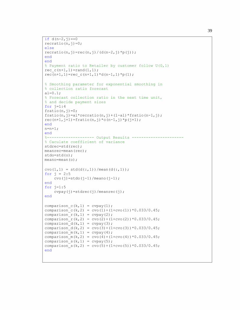
Appendix
Matlab Code for Extended Beer Distribution Game Model
%--------------------Initialization---------------------- % Number of total time periods in the simulation for k=1:1000 N=121;
clear inv d o onorder bo f clear nn index rand1 clear rec recratio fratio cv % Assigning initial values % inv: inventory level % bo: backorder amount % onorder: inventory on order % d: demand to a SC member from its downstream member % o: order placed by a SC member to its upstream member % f: order-up-to level % rec: collection of sales % recratio: collection ratio % fratio: forecasted collection ratio for j=1:5 for n=1:20 inv(n,j)=100; bo(n,j)=0; onorder(n,j)=0; d(n,j)=0; f(n,j)=0; o(n,j)=0; rec(n,j)=0; recratio(n,j)=0; fratio(n,j)=0; end end % Prices p(1)=2; p(2)=1.75; p(3)=1.5; p(4)=1.25; p(5)=1;
% Lead time for j=1:5 t(j)=5; end

38
% Generate normally distributed customer demand a = 0; b = 1000; c =100; nn = N*2;mm = 50; x = randn(1,nn); x = x/std(x)*sqrt(c); x = x -mean(x)+mm; index = find(x>=a & x<=b); rand1= fix(x(index)); %----------------------- Simulation------------------------ while n<N for j=1:4 % Receive products and update inventory level inv(n,j)=inv(n-1,j)-bo(n-1,j)+o(n-t(j+1),j)-d(n-1,j); if inv(n,j)<0 bo(n,j)=0-inv(n,j); inv(n,j)=0; else bo(n,j)=0; end end % Forecast demand by moving average for j=1:4 s(n,j)=0; for i=1:9 s(n,j)=s(n,j)+d(n-i,j); end f(n,j)=s(n,j)/9; end % Calculate inventory on order
for j=1:4 onorder(n,j)=0; for i=1:t(j+1)-1 onorder(n,j)=onorder(n,j)+o(n-i,j); end end % Decide order size by order-up-to policy for j=1:4 if inv(n-1,j)-d(n-1,j)-bo(n-1,j)+o(n-
t(j+1),j)+onorder(n,j)<t(j+1)*f(n,j) o(n,j)=t(j+1)*f(n,j)-(inv(n-1,j)-d(n-1,j)-bo(n-1,j)+o(n-
t(j+1),j)+onorder(n,j)); else o(n,j)=0; end end % Generate place orders to upstream member % Demand to the Retailer d(n,1)=rand1(n); % Demand to each member is exactly the orders placed by % its downstream member for j=2:5 d(n,j)=o(n,j-1); end % Calculate the collection ratio at current time unit for j=1:5
39
if d(n-2,j)==0 recratio(n,j)=0; else recratio(n,j)=rec(n,j)/(d(n-2,j)*p(j)); end end % Payment ratio to Retailer by customer follow U(0,1) rec_c(n+1,1)=rand(1,1); rec(n+1,1)=rec_c(n+1,1)*d(n-1,1)*p(1);
% Smoothing parameter for exponential smoothing in % collection ratio forecast al=0.1; % Forecast collection ratio in the next time unit, % and decide payment sizes for j=1:4 fratio(n,j)=0; fratio(n,j)=al*recratio(n,j)+(1-al)*fratio(n-1,j); rec(n+1,j+1)=fratio(n,j)*o(n-1,j)*p(j+1); end n=n+1; end %-------------------- Output Results ---------------------- % Caculate coefficient of variance stdrec=std(rec); meanrec=mean(rec); stdo=std(o); meano=mean(o);
cvo(1,1) = std(d(:,1))/mean(d(:,1)); for j = 2:5 cvo(j)=stdo(j-1)/meano(j-1); end for j=1:5 cvpay(j)=stdrec(j)/meanrec(j); end
comparison_c(k,1) = cvpay(1); comparison_c(k,2) = cvo(1)+(1+cvo(1))*0.033/0.45; comparison_r(k,1) = cvpay(2); comparison_r(k,2) = cvo(2)+(1+cvo(2))*0.033/0.45; comparison_d(k,1) = cvpay(3); comparison_d(k,2) = cvo(3)+(1+cvo(3))*0.033/0.45; comparison_m(k,1) = cvpay(4); comparison_m(k,2) = cvo(4)+(1+cvo(4))*0.033/0.45; comparison_s(k,1) = cvpay(5); comparison_s(k,2) = cvo(5)+(1+cvo(5))*0.033/0.45; end