simulation modeling approach for evaluating a solution
TRANSCRIPT
University of Arkansas, FayettevilleScholarWorks@UARK
Theses and Dissertations
8-2017
Simulation Modeling Approach for Evaluating aSolution Designed to Alleviate the Congestion ofPassenger Flow at the Composure Area of SecurityCheckpointsMaria Luisa Janer RubioUniversity of Arkansas, Fayetteville
Follow this and additional works at: http://scholarworks.uark.edu/etd
Part of the Industrial Engineering Commons, Industrial Technology Commons, and theTransportation Commons
This Thesis is brought to you for free and open access by ScholarWorks@UARK. It has been accepted for inclusion in Theses and Dissertations by anauthorized administrator of ScholarWorks@UARK. For more information, please contact [email protected], [email protected].
Recommended CitationJaner Rubio, Maria Luisa, "Simulation Modeling Approach for Evaluating a Solution Designed to Alleviate the Congestion ofPassenger Flow at the Composure Area of Security Checkpoints" (2017). Theses and Dissertations. 2448.http://scholarworks.uark.edu/etd/2448
Simulation Modeling Approach for Evaluating a Solution Designed to Alleviate the Congestion
of Passenger Flow at the Composure Area of Security Checkpoints
A thesis submitted in partial fulfillment
of the requirements for the degree of
Master of Science in Industrial Engineering
by
Maria Luisa Janer Rubio
University of Arkansas
Bachelor of Science in Industrial Engineering, 2015
August 2017
University of Arkansas
This thesis is approved for recommendation to the Graduate Council.
_____________________________________
Dr. Manuel Rossetti
Thesis Director
____________________________________ _____________________________________
Dr. Richard Ham Dr. Shengfan Zhang
Committee Member Committee Member
Abstract
In a previous study, we found that replacing the exit roller of a security checkpoint lane
for a continuously circulating conveyor could potentially increase the throughput of passengers
by over 28% while maintaining the TSA security-waiting time limit (Janer and Rossetti 2016).
This study intends to expand this previous effort by investigating the impact of this circulating
conveyor on the secondary screening related processes. Leone and Liu (2011) found that
imposing a limit on the x-ray screening time, and diverting any item exceeding this limit to
secondary screening, could decrease the waiting time by 43%. Our objective is to verify Leone
and Lui’s findings using discrete event simulation, and evaluate the effect of a circulating
conveyor on these findings. In particular, we intend to optimize univariate response curves of
the same response variable in Leone and Liu’s effort. Simulation will be used to evaluate the
optimal solution, and investigate the possibility of replacing a traditional two-lane system with a
single lane having the circulating conveyor in place.
©2017 by Maria Luisa Janer Rubio
All Rights Reserved

Acknowledgements
I extend a special thanks to my faculty advisor, Dr. Manuel Rossetti, for his support, time
and long hours invested on this study. It could not have been possible without you.
Table of Contents
I. INTRODUCTION ................................................................................................................. 1
II. LITERATURE REVIEW ................................................................................................. 4
III. SYSTEM DEFINITION .................................................................................................. 12
Solution Prototype 1 ................................................................................................................ 14
Solution Prototype 2 ................................................................................................................ 16
IV. MODELS’ IMPLEMENTATION .................................................................................. 17
Divestiture Modeling ............................................................................................................... 17
Composure Modeling in the Current Configuration Model ............................................... 18
Composure Modeling of the Circulating Conveyor ............................................................. 21
Secondary Screening ............................................................................................................... 22
V. MODEL ESTIMATION OF PARAMETERS.................................................................. 24
Data Collection on Arrival Patterns ...................................................................................... 25
Data Collection on Inspection Times at the X-Ray and Secondary Screening .................. 29
Data Collection on Passengers’ System Times and Throughput ........................................ 30
Data Collection on the Distribution for the Number of Items per Passenger ................... 32
VI. MODELS’ VALIDATION AND VERIFICATION ..................................................... 33
VII. EXPERIMENTATION AND RESULTS ...................................................................... 35
Threshold on the X-Ray Processing Time Limit .................................................................. 37
Threshold on the Number of Items per Passenger ............................................................... 51
Replacing a Traditional Two Lane System with One Circulating Conveyor Lane .......... 57
CONCLUSION AND FUTURE WORK .................................................................................. 61
REFERENCES ............................................................................................................................ 65
APPENDIX .................................................................................................................................. 67

List of Figures
Figure 1. TSA Security Checkpoint Layout ................................................................................. 13
Figure 2. Solution Prototype 1 Layout .......................................................................................... 15
Figure 3. Solution Prototype 2 Layout .......................................................................................... 16
Figure 4. Passenger Volume per day of the week ......................................................................... 26
Figure 5. Passenger Volume per hour of the day .......................................................................... 26
Figure 6. Number of Lanes Open per Hour of the Day ................................................................ 28
Figure 7. Arrival Patterns and Lane Idle Capoacity at a Larger Airport in Western Europe ....... 28
Figure 8. X-Ray Screening Inspection Times ............................................................................... 29
Figure 9. System Time of Passengers on Monday ........................................................................ 30
Figure 10. System Time of Passengers from Tuesday to Thursday ............................................. 31
Figure 11. System Time of Passengers on Saturday ..................................................................... 31
Figure 12. System Time of Passenger on Sunday......................................................................... 31
Figure 13. Throughput and relative number of passengers with manual baggage inspection ...... 32
Figure 14. Animation of Base Configuration Model .................................................................... 34
Figure 15. Animation of the Prototype 1 Model ............................ Error! Bookmark not defined.
Figure 16. Animation of Second Prototype Model ....................................................................... 35
Figure 17. Response to Change in the X-Ray Processing Time Limit (Base Model) .................. 38
Figure 18. Probability that the Diverter Roller is full ................................................................... 39
Figure 19. Residuals Analysis on System Time vs. X-ray PT Limit (Base Model and CV = 0.71)
....................................................................................................................................................... 40
Figure 20. Tuckey's Multiple Comparisons on System Time vs. X-ray PT Limit (Base Model CV
= 0.71) ........................................................................................................................................... 40
Figure 21. Polynomial Regression on Base Model (CV = 0.71) .................................................. 42
Figure 22. Response Curve on Base Model (CV = 0.5) ............................................................... 44
Figure 23. Response Curve on Base Model (CV = 1.0) ............................................................... 44
Figure 24. Response Curve on Base Model (CV = 1.5) ............................................................... 45
Figure 25. Multiple Comparison on System Time vs. Coefficient of Variation (Base Model and
Optimum X-Ray PT Limit) ........................................................................................................... 47
Figure 26. Residuals Analysis on System Time vs. Coefficient of Variation (Base Model and
Optimum X-Ray PT Limit) ........................................................................................................... 47
Figure 27. Response Curve for Prototype 1 Model (CV = 0.71) .................................................. 48
Figure 28. Response Curve for Prototype 2 Model (CV = 0.71) .................................................. 48
Figure 29. Residuals Analysis on System Time vs. Models (CV = 0.71 and Optimum X-Ray PT
Limit) ............................................................................................................................................ 50
Figure 30. Multiple Comparison on System Time vs. Models (CV = 0.71 and Optimum X-Ray
PT Limit) ....................................................................................................................................... 50
Figure 31. Interval Plot on System Time vs. Num. of Items Threshold (High-Traffic Volume
Distribution) .................................................................................................................................. 53
Figure 32. Multiple Comparison Test on System Time vs. Num. of Items Threshold (High-
Traffic Volume Distribution) ........................................................................................................ 54
Figure 33. Interval Plot on System Time vs. Num. of Items Threshold (Medium-Traffic Volume
Distribution) .................................................................................................................................. 55
Figure 34. Multiple Comparison Test on System Time vs. Num. of Items Threshold (Medium-
Traffic Volume Distribution) ........................................................................................................ 55
Figure 35. Interval Plot on System Time vs. Num. of Items Threshold (Low-Traffic Volume
Distribution) .................................................................................................................................. 56
Figure 36. Multiple Comparison Test on System Time vs. Num. of Items Threshold (Low-Traffic
Volume Distribution) .................................................................................................................... 57
Figure 37. AIT Throughput vs. Arrival Rate ................................................................................ 59
Figure 38. Prob. Time to Composure Less Than 10 min. vs. Arrival Rate .................................. 59
Figure 39. Total System Time vs. Arrival Rate ............................................................................ 60
Figure 40. ANOVA on System Time vs. X-ray PT Limit Levels (Base Model and CV = 0.71) . 67
Figure 41. Multiple Comparisons on System Time vs. X-ray PT Limit Levels (Base Model and
CV = 0.71) .................................................................................................................................... 67
Figure 42. ANOVA on System Time vs. Coefficient of Variation (Base Model and Optimum X-
Ray PT Limit) ............................................................................................................................... 69
Figure 43. ANOVA on System Time vs. Models (CV = 0.71 and Optimum X-Ray PT Limit) .. 71
Figure 44. Multiple Comparison Test on System Time vs. Models (CV = 0.71 and Optimum X-
Ray PT Limit) ............................................................................................................................... 71
List of Exhibits
Exhibit 1. Separate Passengers from Items Logic ........................................................................ 18
Exhibit 2.Divestiture Process Logic ............................................................................................. 18
Exhibit 3. Logic for Item Rolling on Exit Roller .......................................................................... 19
Exhibit 4. Passenger Collecting Items Logic ................................................................................ 20
Exhibit 5. Passenger Logic for Composure in a Circulating Conveyor Lane ............................... 21
Exhibit 6. Item Logic for Composure in a Circulating Conveyor Lane ....................................... 22
Exhibit 7. Item Logic on Diverter Roller ...................................................................................... 23
Exhibit 8. Item Logic on Diverter Roller ...................................................................................... 24
List of Tables
Table 1.Earliness of Arrival Profile at Seattle-Tacoma International Airport .............................. 25
Table 2. Arrival Schedule from 5:00 am to 11:00 pm .................................................................. 27
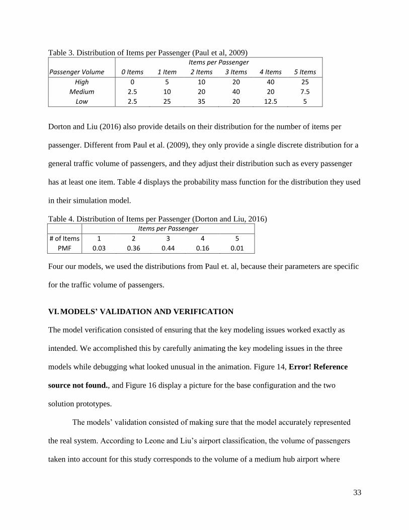
Table 3. Distribution of Items per Passenger (Paul et al, 2009) ................................................... 33
Table 4. Distribution of Items per Passenger (Dorton and Liu, 2016) ......................................... 33
Table 5. Experiment Design for ANOVA on X-Ray PT Limit. ................................................... 39
Table 6. ANOVA and Regression Statistics ................................................................................. 43
Table 7. Statistical Significance of Regression in Figure 22 ........................................................ 68
Table 8. Statistical Significance of Regression in Figure 23 ........................................................ 68
Table 9. Statistical Significance of Regression in Figure 17 ........................................................ 69
Table 10. Significance of Regression Model in Figure 27 ........................................................... 70
Table 11. Significance of Regression in Figure 28 ....................................................................... 70
1
I. INTRODUCTION
As the world has progressively transformed into an integrated global economy, air transportation
has become one of the most fundamental means to connect people in distant places. Revenue
Passenger Miles (RPMs) is the aviation standard for measuring air travel volume. It represents
one paying passenger travelling one mile. The U.S. Department of Transportation’s Federal
Aviation Administration’s (FAA) projected in 2013 that U.S. carriers RPMs will grow 76% by
2034, and the number of people flying per year will increase from 745.5 million in 2014 to 1.15
billion in 2034 (Price 2014).
One of the major concerns is the U.S. airports’ infrastructure available to sustain this
growth. Prior to September 11, 2001, there was no concrete process to screen checked luggage.
In fact, only 5% of the checked bags were investigated (Blalock 2007). In 2002, the
Transportation Security Administration (TSA) mandated to begin screening 100% of the checked
luggage (Mead 2003). This involved installing explosive detection system machines of the size
of sport utility vehicles and massive conveyor systems across all U.S. commercial airports
(Blalock 2007). This left very little space to accommodate passenger screening procedures, and
possible future growth of passenger traffic. Consequently, passenger-screening operations have
become one of the major bottlenecks among airport operations today (Blalock 2007).
In an effort to provide solutions to the major causes of constrained flow, several studies
have identified the x-ray as the main impediment of continuous traffic of passengers and items
(De Barros and Tomber 2007). A study performed at the Dallas/Fort Worth International Airport
(DFW) attributed this to the processes of divestiture and composure, happening before and after
the x-ray, respectively (DFW Planning Department 2005). Regarding divestiture, the problem
resides with passengers waiting until they have reached the divestiture tables to start preparing
2
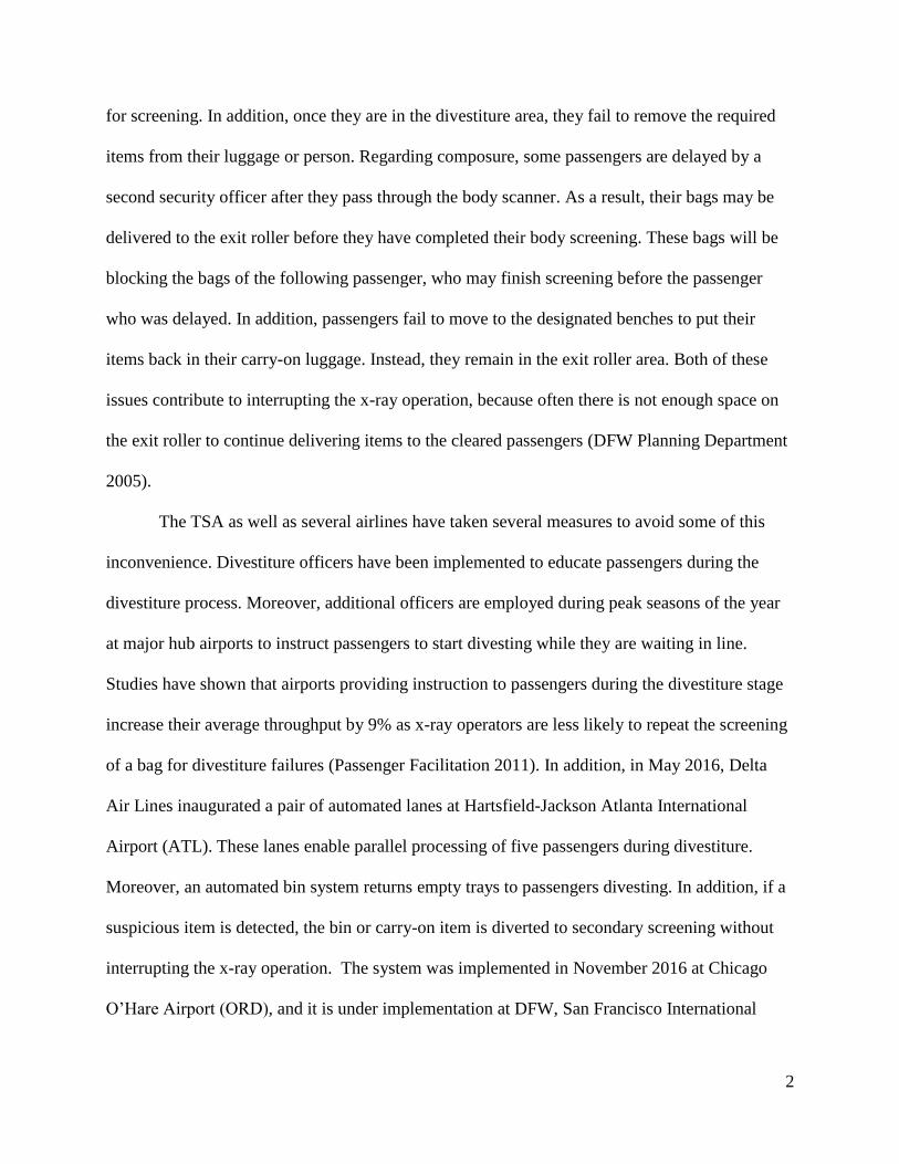
for screening. In addition, once they are in the divestiture area, they fail to remove the required
items from their luggage or person. Regarding composure, some passengers are delayed by a
second security officer after they pass through the body scanner. As a result, their bags may be
delivered to the exit roller before they have completed their body screening. These bags will be
blocking the bags of the following passenger, who may finish screening before the passenger
who was delayed. In addition, passengers fail to move to the designated benches to put their
items back in their carry-on luggage. Instead, they remain in the exit roller area. Both of these
issues contribute to interrupting the x-ray operation, because often there is not enough space on
the exit roller to continue delivering items to the cleared passengers (DFW Planning Department
2005).
The TSA as well as several airlines have taken several measures to avoid some of this
inconvenience. Divestiture officers have been implemented to educate passengers during the
divestiture process. Moreover, additional officers are employed during peak seasons of the year
at major hub airports to instruct passengers to start divesting while they are waiting in line.
Studies have shown that airports providing instruction to passengers during the divestiture stage
increase their average throughput by 9% as x-ray operators are less likely to repeat the screening
of a bag for divestiture failures (Passenger Facilitation 2011). In addition, in May 2016, Delta
Air Lines inaugurated a pair of automated lanes at Hartsfield-Jackson Atlanta International
Airport (ATL). These lanes enable parallel processing of five passengers during divestiture.
Moreover, an automated bin system returns empty trays to passengers divesting. In addition, if a
suspicious item is detected, the bin or carry-on item is diverted to secondary screening without
interrupting the x-ray operation. The system was implemented in November 2016 at Chicago
O’Hare Airport (ORD), and it is under implementation at DFW, San Francisco International

3
Airport (SFO) and Los Angeles International Airport (LAX) (Solomon 2016). Similarly, the Pre-
Check program, introduced in 2013, is increasingly growing. It was established to improve the
experience and security benefit of known travelers and the overall checkpoint performance. As
of September 2015, 1.6 million individuals have enrolled, and the TSA estimates the number
could rise to 25 million by 2020 if they focus the program marketing on the private sector (TSA
Pre-Check Expansion Act 2016).
Despite these improvements, the long waiting lines remain a concern, especially for the
peak seasons of the year. In 2016, the TSA experienced a shortage of screeners as they reduced
the staff by 12% since 2013 due to federal budget cuts. On the other hand, summer passenger
traffic has increased by 15% since the summer of 2013 (Davis 2016). Consequently, in May
2016, passengers experienced waiting times of up to 50 minutes in major airports, including
DFW, SFO and ATL. As a result, the TSA employed private security screeners, and intensified
the use of security dogs to aid the screening of passengers for the rest of the summer (Quintana
and Sze 2016).
This research aims to evaluate a solution designed to alleviate the long waiting lines
caused by seasonal travelers. We address specifically the issues at composure where some
passengers can block the way of other passengers if they are delayed after the body screening.
We investigate the possibility of implementing a continuously circulating conveyor on place of
the exit roller of one of the checkpoint lanes. We use discrete event simulation (DES) to evaluate
the effect of this circulating conveyor on the x-ray screening and secondary manual screening.
We use the professional version 15 of Arena Rockwell Software as the simulation software of
this study.

4
This paper is organized as follows: in Section 2, we review the efforts found in the
literature on improving the performance of security checkpoints using DES or analytics. In
Section 3, we describe in detail the system under study, and the solution prototypes. In Section 4,
we illustrate the conceptual modeling, and the key constructs used to implement the simulation
models. In Section 5, we summarize the efforts used to obtain the distribution parameters for the
models. In Section 6, we explain in detail how we verified and validated the models. In Section
7, we explain the experimentation methods and results obtained from evaluating the models.
II. LITERATURE REVIEW
As we are trying to evaluate a solution that can benefit both the security of passengers and the
passenger flow, we reviewed studies focusing on both or either of these two aspects. Several
studies concentrate on diagnosing causes of passenger flow congestion or investigating the
interrelation between variables having an effect on the checkpoint throughput performance. De
Barros and Tomber (2007) evaluated and quantified the impact of post 9/11 security measures on
the planning and operations of airport terminals. They built a spreadsheet model based on
deterministic querying theory to obtain estimates of the queue length and approximate waiting
times at the passenger screening. Moreover, they used a simulation model built in Arena to
evaluate seven scenarios associated with the different measures implemented after 9/11. Their
findings assert that reducing the number of carry-on items to one item per passenger was the
most effective measure to reduce the waiting time of passengers. In addition, adding pre-
screening tables for passengers to divest helped reducing the waiting time by almost two thirds.
Moreover, they compare the different methods available to analyze security checkpoints. As they
explain, in the absence of data, a mathematical model can provide meaningful insights about the
interrelationships between variables and service components. Despite this contribution, they fail
5
to explain their definition for waiting time. In addition, it is impossible to qualify their models as
realistic as they provide no detail about the assumptions made to implement the analytic and
simulation models.
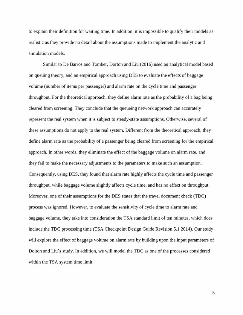
Similar to De Barros and Tomber, Dorton and Liu (2016) used an analytical model based
on queuing theory, and an empirical approach using DES to evaluate the effects of baggage
volume (number of items per passenger) and alarm rate on the cycle time and passenger
throughput. For the theoretical approach, they define alarm rate as the probability of a bag being
cleared from screening. They conclude that the queueing network approach can accurately
represent the real system when it is subject to steady-state assumptions. Otherwise, several of
these assumptions do not apply to the real system. Different from the theoretical approach, they
define alarm rate as the probability of a passenger being cleared from screening for the empirical
approach. In other words, they eliminate the effect of the baggage volume on alarm rate, and
they fail to make the necessary adjustments to the parameters to make such an assumption.
Consequently, using DES, they found that alarm rate highly affects the cycle time and passenger
throughput, while baggage volume slightly affects cycle time, and has no effect on throughput.
Moreover, one of their assumptions for the DES states that the travel document check (TDC)
process was ignored. However, to evaluate the sensitivity of cycle time to alarm rate and
baggage volume, they take into consideration the TSA standard limit of ten minutes, which does
include the TDC processing time (TSA Checkpoint Design Guide Revision 5.1 2014). Our study
will explore the effect of baggage volume on alarm rate by building upon the input parameters of
Dolton and Liu’s study. In addition, we will model the TDC as one of the processes considered
within the TSA system time limit.
6
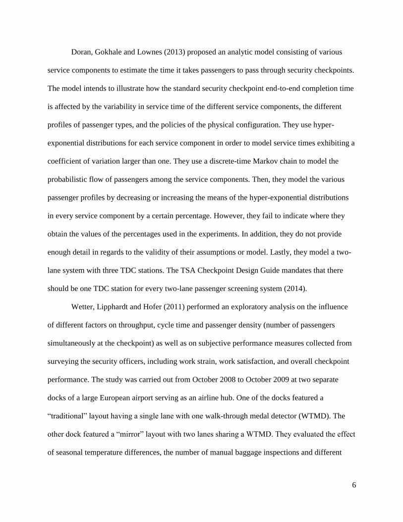
Doran, Gokhale and Lownes (2013) proposed an analytic model consisting of various
service components to estimate the time it takes passengers to pass through security checkpoints.
The model intends to illustrate how the standard security checkpoint end-to-end completion time
is affected by the variability in service time of the different service components, the different
profiles of passenger types, and the policies of the physical configuration. They use hyper-
exponential distributions for each service component in order to model service times exhibiting a
coefficient of variation larger than one. They use a discrete-time Markov chain to model the
probabilistic flow of passengers among the service components. Then, they model the various
passenger profiles by decreasing or increasing the means of the hyper-exponential distributions
in every service component by a certain percentage. However, they fail to indicate where they
obtain the values of the percentages used in the experiments. In addition, they do not provide
enough detail in regards to the validity of their assumptions or model. Lastly, they model a two-
lane system with three TDC stations. The TSA Checkpoint Design Guide mandates that there
should be one TDC station for every two-lane passenger screening system (2014).
Wetter, Lipphardt and Hofer (2011) performed an exploratory analysis on the influence
of different factors on throughput, cycle time and passenger density (number of passengers
simultaneously at the checkpoint) as well as on subjective performance measures collected from
surveying the security officers, including work strain, work satisfaction, and overall checkpoint
performance. The study was carried out from October 2008 to October 2009 at two separate
docks of a large European airport serving as an airline hub. One of the docks featured a
“traditional” layout having a single lane with one walk-through medal detector (WTMD). The
other dock featured a “mirror” layout with two lanes sharing a WTMD. They evaluated the effect
of seasonal temperature differences, the number of manual baggage inspections and different
7
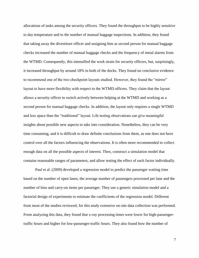
allocations of tasks among the security officers. They found the throughput to be highly sensitive
to day temperature and to the number of manual baggage inspections. In addition, they found
that taking away the divestiture officer and assigning him as second person for manual baggage
checks increased the number of manual baggage checks and the frequency of metal alarms from
the WTMD. Consequently, this intensified the work strain for security officers, but, surprisingly,
it increased throughput by around 18% in both of the docks. They found no conclusive evidence
to recommend one of the two checkpoint layouts studied. However, they found the “mirror”
layout to have more flexibility with respect to the WTMD officers. They claim that the layout
allows a security officer to switch actively between helping at the WTMD and working as a
second person for manual baggage checks. In addition, the layout only requires a single WTMD
and less space than the “traditional” layout. Life testing observations can give meaningful
insights about possible new aspects to take into consideration. Nonetheless, they can be very
time consuming, and it is difficult to draw definite conclusions from them, as one does not have
control over all the factors influencing the observations. It is often more recommended to collect
enough data on all the possible aspects of interest. Then, construct a simulation model that
contains reasonable ranges of parameters, and allow testing the effect of each factor individually.
Paul et al. (2009) developed a regression model to predict the passenger waiting time
based on the number of open lanes, the average number of passengers processed per lane and the
number of bins and carry-on items per passenger. They use a generic simulation model and a
factorial design of experiments to estimate the coefficients of the regression model. Different
from most of the studies reviewed, for this study extensive on-site data collection was performed.
From analyzing this data, they found that x-ray processing times were lower for high-passenger-
traffic hours and higher for low-passenger-traffic hours. They also found how the number of
8
items per passenger vary significantly with time of the day and day of the week. They observed
the highest number of items per passenger in the morning hours during weekdays, when most
travelers are business passengers. In addition, the results of their simulation model show that the
factors with highest impact on waiting time are passenger volume, number of items per
passenger, number of lanes open and staff level. Their efforts on data collection will be
summarized in Section 5.
Other studies were intended to develop templates to aid the simulation analysis of
security checkpoint systems. Guru and Savory (2004) described their effort in developing an
internet-based application to assist a simulation analyst in the conceptual modeling stage of
security screening systems. The application consists of 15 templates of the security equipment,
intended to help identify the important input modeling parameters, the system components and
the interrelationships among the various components and parameters. Although the templates can
give meaningful insights in regards to the security equipment, the study fails to illustrate how
passengers, security officers, and the material handling are taken into account in their templates.
Fayetz et al. (2008) developed a decision support tool based on simulation designed to
assess the current state of airports’ functional areas as well as the impact of new procedures on
space allocation per passenger and waiting times at the different processing points. The tool
allows the modeling of new procedures by providing a simple framework to change the
distribution parameters associated with each functional area. Thus, the tool can be very useful for
evaluating small alterations for which one can instinctively predict the differences in the
distribution. However, for more complex changes for which one cannot instinctively predict the
differences in the distribution, it seems one must replicate the changes in real life in order to
9
collect the data for the new input parameters, and have the tool accurately predict the impact of
such changes.
Wilson, Roe and So (2006) present the Security Checkpoint Optimizer (SCO), a java-
based DES tool developed by Northrop Group for the TSA. Similar to the tool presented by
Fayetz et al., the SCO is spatially aware, and it was designed to evaluate passenger and lugagge
throughput, security effectiveness, resource utilization and operational costs. Nonetheless, it
contains a novel 2-D animation, enabling the user to verify the modeling of procedures
implemented. In addition, it allows evaluating the security effectiveness by aggregating
probabilities of detection for some item of interest.
Pendegraft, Robertson and Shrader (2004) present a DES model developed to evaluate
new policies in the passenger and luggage screening systems at Baltimore Washington
International Airport. Although they do not provide much detail in regards to the simulation
model, they describe a step-by-step procedure for estimating arrival rate parameters from flight
departure schedules. A detailed description of this contribution is presented in Section 5. In
addition, they include the modeling of processes such as check-in and passenger boarding to
represent accurately the impact that such processes have on the security checkpoint demand. The
model was used to recommend resource requirements (x-rays, metal detectors, ETDs, and
officers) in all the major hub airports in the United States.
Similar to our study, other efforts focus on proposing and evaluating the effectiveness of
solutions to issues already identified. Leone and Liu (2011) observed that while 80% of the items
are inspected within 7 seconds in the primary screening, a lengthy right tail in the distribution of
the inspection time implies that a very small proportion of items are disproportionately
contributing to decreasing the inspection rate and the overall checkpoint performance. They
10
propose that imposing a limit in the primary screening inspection time and increasing the
rejection rate to secondary screening of items taking longer than that limit would improve the
throughput and overall waiting time of passengers. Using queuing and simulation models, they
assert their solution decreases the mean waiting time by 43%, reduces the operation costs by 1%,
and increases the probability of detecting a prohibited item to 10%. Nonetheless, it is not clear
how obtain these two last conclusions, as they do not provide any detail about how they
estimated operation costs and the probability of detecting a threat. Furthermore, similar to Dolton
and Liu (2016), with their models, they obtain waiting times of above 12 minutes without
modeling the TDC process. On the other hand, one contribution of this study is the detailed
explanation on the data collection methods and parameters obtained for their models. This
contribution will be discussed further in Section 5.
De Lange et al. (2013) investigate the possibility of implementing virtual queuing at
security checkpoints by offering to some passengers a time window during which they can
bypass the TDC queue, and have priority to access the security lanes. They implemented a DES
model of a large international airport in Western Europe to determine whether virtual queueing
could reduce the number of agents at security lanes while not increasing the average passenger
waiting time. The essence of this solution consists of redistributing the passenger arrivals by
shifting the checkpoint demand out of peak periods into de idle periods. They evaluated twelve
different infinite horizon simulations of 100 days each to determine the optimal time window
(TW) and the best time a passenger could be moved later in time (i.e. the best transfer time limit
- TTL). Then, using the optimal TTL and TW, using four additional scenarios, they perform a
sensitivity analysis on the participation level of passengers to determine the ultimate benefit of
the solution. They conclude that the effectivity of the virtual queuing solution would depend on

11
the reliability of the forecasting method, the arrival rate pattern, the number of eligible
passengers, and the length of the TWs. They found that this solution works best for airports with
arrival rate patterns displaying sharp and frequent peaks exceeding the checkpoint capacity,
followed by periods of light passenger traffic. Considering virtual queuing allows reducing the
number of security lanes required, they found that at least 60% of the eligible passengers must
participate of the program to preserve the benefits of the solution. In addition, the TW should be
kept as short as possible to maximize the transfer accuracy rate, as this ensures higher utilization
of the idle capacity. Different from our study, De Lange et al. do not study the impact of the
solution on security. Nonetheless, similar to our experiment design, their study consists of a
series of sensitivity analysis on the input parameters of the solution.
The last set of reviewed studies provide some insights in regards to the assignment of
passenger types based on the state of the system. Nie et al. (2011) investigate a solution to utilize
effectively the Selectee Lane, which has more strict screening procedures than a normal lane, in
order to maximize the probability of true alarm. They assume a prior prescreening process at the
check-in assigns passengers into different risk classes according to the passengers’ perceived risk
levels. Consequently, they propose assigning the different risk classes to the Selectee Lane based
on the number of passengers that are already in the lane. First, they study a steady-state model
and formulate it as a nonlinear binary integer program. Next, they find an approximate solution
to this model using a rule-based heuristic. Later, they explore the solution obtained using a
simulation framework designed to evaluate different assignment solutions. Lastly, they use a
neighborhood search procedure to derive assignment solutions with better performance from the
initial heuristic solution, and evaluate the derived solutions using the simulation framework. The
main contribution of this work to our study lays on the way the rule-based heuristic is formulated
12
to guarantee solutions that maximize the objective of the study. For our purpose, we will
formulate a similar rule-based heuristic to obtain an assignment solution that minimizes the
passengers’ waiting time. Nonetheless, Nie et al. do not provide any statistical support for their
selection of running parameters for the simulation model. Moreover, it is not clear what type of
horizon they use for their simulation framework.
III. SYSTEM DEFINITION
This section presents the system under study and the two prototypes of the solution that will be
evaluated against the current configuration.
Our system consists of the passenger security-screening checkpoint, including
passengers, security officers, material handling and security equipment. It extends from where
passengers join a line to have their documents checked by a TDC officer until they have
collected their last item from either the exit roller or the secondary screening station. The system
is modeled according to the standards in the Revision 5.1 of the TSA Checkpoint Design Guide
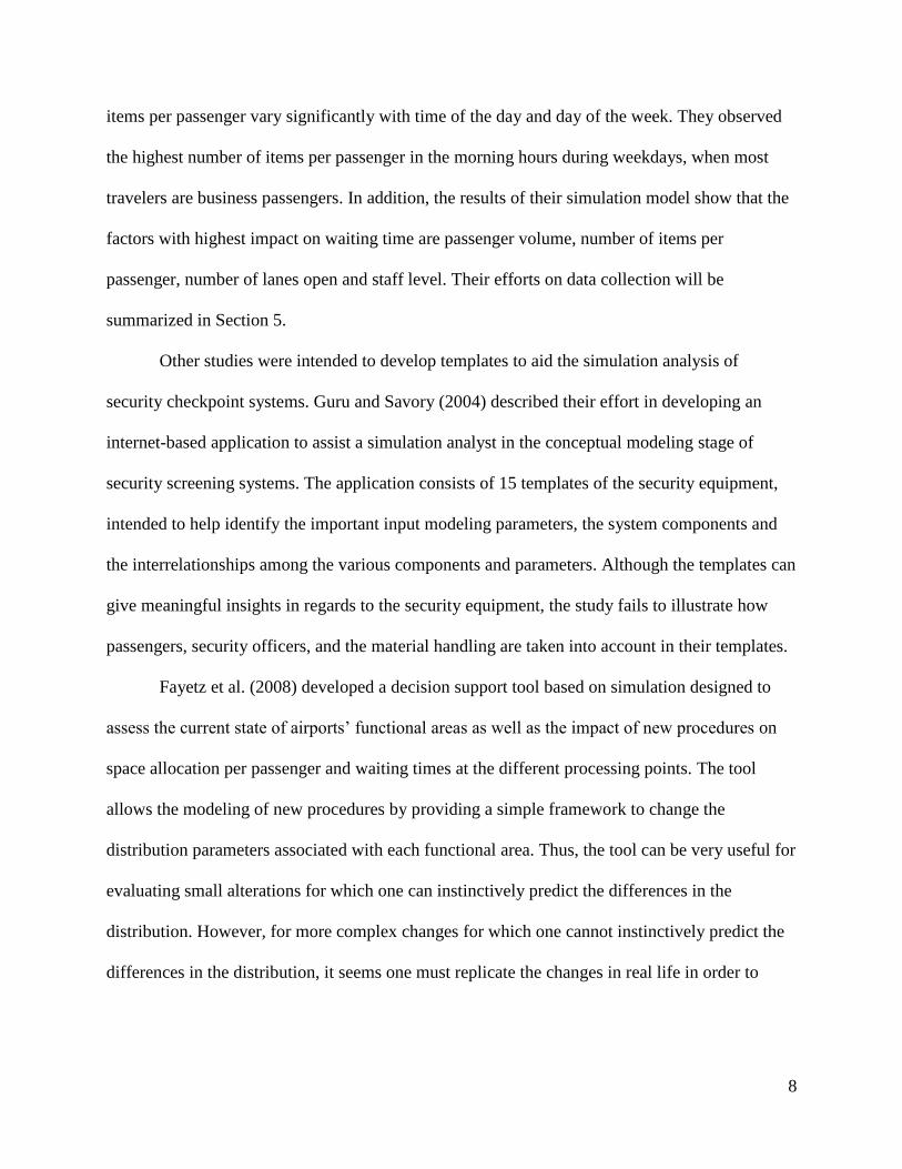
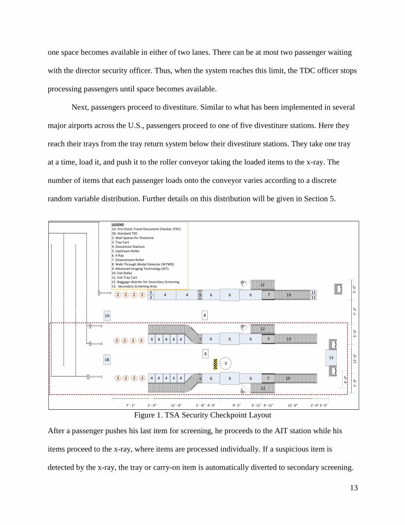
(2014). Figure 1 displays a layout of the system elements under study encircled in red.
Following advice from TSA design agents, we studied a two-lane mirror layout where
two lanes share one WTMD, one advanced imaging technology (AIT) and one secondary
screening station. Note we do not include in the system the Pre-Check lane, depicted above the
dashed lane, or the processing of Pre-Check passengers.
Upon arrival, standard passengers join the queue for verifying their documents with a
TDC officer. After the TDC officer has finished reviewing the passenger’s documents, a
different security officer directs the passenger to the lane with the smaller number of passengers
waiting. There can be at most four passengers per lane waiting for divestiture. Thus, if there is
not a space available in any of the two lanes, the passenger stays with the director officer until
13
one space becomes available in either of two lanes. There can be at most two passenger waiting
with the director security officer. Thus, when the system reaches this limit, the TDC officer stops
processing passengers until space becomes available.
Next, passengers proceed to divestiture. Similar to what has been implemented in several
major airports across the U.S., passengers proceed to one of five divestiture stations. Here they
reach their trays from the tray return system below their divestiture stations. They take one tray
at a time, load it, and push it to the roller conveyor taking the loaded items to the x-ray. The
number of items that each passenger loads onto the conveyor varies according to a discrete
random variable distribution. Further details on this distribution will be given in Section 5.
Figure 1. TSA Security Checkpoint Layout
After a passenger pushes his last item for screening, he proceeds to the AIT station while his
items proceed to the x-ray, where items are processed individually. If a suspicious item is
detected by the x-ray, the tray or carry-on item is automatically diverted to secondary screening.
8
8
1A
1B9
2 5 7 10
LEGEND1A. Pre-Check Travel Document Checker (TDC)1B. Standard TDC2. Wait Spaces for Divesture3. Tray Cart4. Divestiture Stations5. Upstream Roller6. X-Ray7. Downstream Roller8. Walk Through Medal Detector (WTMD)9. Advanced Imaging Technology (AIT)10. Exit Roller11. Exit Tray Cart12. Baggage diverter for Secondary Screening13. Secondary Screening Area
6 62 2 2
2 7 1066 62 2 2
34
34
1111
2 7 10662 2 2
13
12
12
10
4 4 4 4 4
4 4 4 4 4
12'-
6"
5'-
0"
5'-
0"
7'-
4"
5'-
0"
1' - 8" 4'- 0" 9'- 5" 3'- 11" 4'- 11"
12
5
5
5
6
2' - 0" 12' - 0"7' - 1" 12'- 0" 2'- 0"
6
3'- 0"
4'-
0"
14
Similarly, if a suspicious item is detected by the AIT, the suspicious passenger is screened by a
second officer with a wander while the following passenger continues through the AIT. The AIT
station becomes available until after the security officer in charge of secondary body screening
becomes available.
After the x-ray screening, cleared items enter a conveyor that delivers the items to the
exit roller in the same order in which the items entered the x-ray. Passengers identify their items
and stay around the exit roller until they have collected all their items. Up to six trays or carry-on
items fit on the exit roller. If there is not a space available for the x-ray operator to continue
delivering cleared trays, the operator stops the x-ray operation until a space opens for a tray to be
delivered. Alarmed items, diverted to the manual diverter roller, are taken individually to a
secondary screening station by a security officer. The security officer advises the passenger to
collect the rest of his cleared items from the exit roller and follow him to the secondary screening
station. The security officer waits for the passenger in the secondary screening station to ensure
that the passenger can see what the officer is doing with the items.
We considered two performance measures to evaluate the performance of the models: the
time to composure and the passenger throughput. The time to composure corresponds to the
period from when passengers join the queue for checking their documents with a TDC officer up
to the time when they are able to pick their items from the exit roller. The TSA has a standard
limit of ten minutes for this measure. The passenger throughput corresponds to the average
number of passengers screened by the AIT, if the system operates at full capacity.
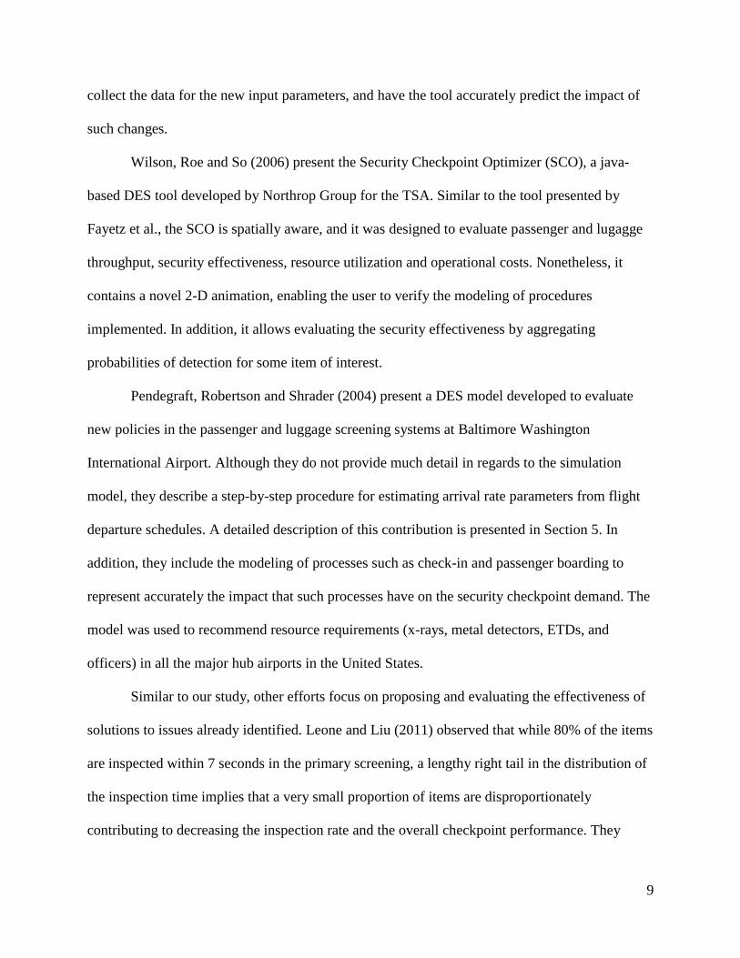
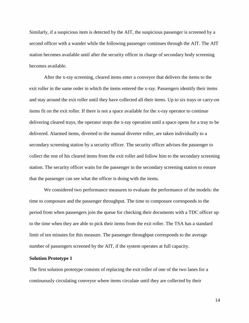
Solution Prototype 1
The first solution prototype consists of replacing the exit roller of one of the two lanes for a
continuously circulating conveyor where items circulate until they are collected by their
15
respective passengers. Figure 2 displays how the layout in Figure 1 would change after this
circulating conveyor is incorporated.
Figure 2. Solution Prototype 1 Layout
After the TDC process, passengers having a number of trays above a specific threshold to be
determined by the experimental analysis are directed to the lane having the circulation conveyor
in place. On the other hand, passengers requiring a number of trays below the threshold are
directed to the lane having the least number of passengers waiting. In the case that both lanes are
even in number of passengers waiting, priority will be given to the lane having the circulating
conveyor.
At most six passengers can be waiting around the conveyor to collect comfortably their
items. It was assumed that passengers avoid running after their items. Thus, upon having been
cleared by the body screening process, passengers proceed to one of these six spaces to wait for
their items. Items are delivered to the conveyor, where they circulate individually, each in one
cell of the conveyor, checking for their passenger in each of the six conveyor spaces. If an item
1' - 8" 4'- 0" 9'- 5" 3'- 11" 4'- 11"2' - 0" 12' - 0"7' - 1"
10'-
0"
7'-
6"
5'-
0"
12'- 0" 2'- 0"
16
identifies a passenger with the same serial number, the item exits the conveyor, and it is put
together with the other passenger’s items. After the last item of the passenger exits the conveyor,
the passenger releases the conveyor waiting space. We assume zero delay in unloading every
item from the conveyor as items will continue circulating if they are not collected
instantaneously.
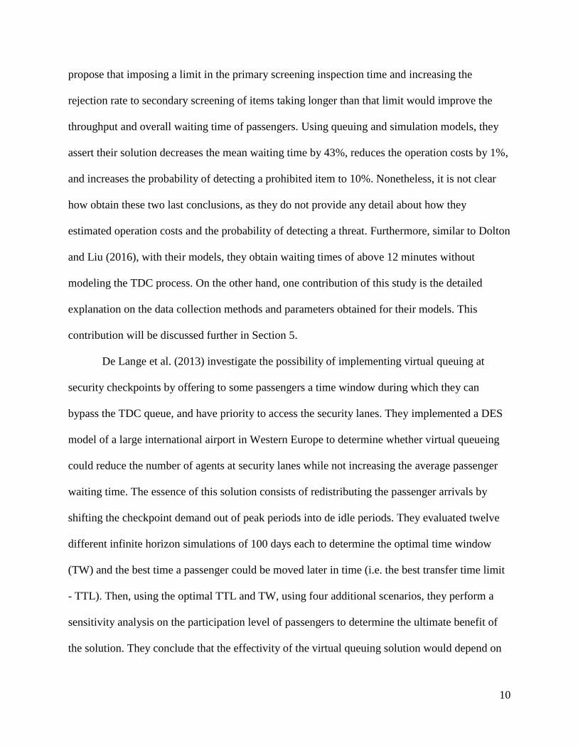
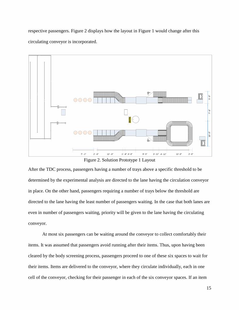
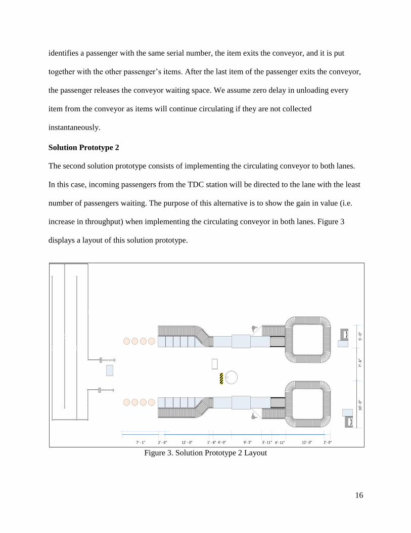
Solution Prototype 2
The second solution prototype consists of implementing the circulating conveyor to both lanes.
In this case, incoming passengers from the TDC station will be directed to the lane with the least
number of passengers waiting. The purpose of this alternative is to show the gain in value (i.e.
increase in throughput) when implementing the circulating conveyor in both lanes. Figure 3
displays a layout of this solution prototype.
Figure 3. Solution Prototype 2 Layout
1' - 8" 4'- 0" 9'- 5" 3'- 11" 4'- 11"2' - 0" 12' - 0"7' - 1"
10
'- 0
"7
'- 6
"5
'- 0
"
12'- 0" 2'- 0"
17
IV. MODELS’ IMPLEMENTATION
Different from a spreadsheet or an analytical model, DES allows capturing the level of detail
necessary for this type of analysis, where the system is subject to non-stationary arrival rates and
variability in the service time parameters. In this section, we explore the key modelling issues to
imitate the real system in a computer for the current configuration and the two solution
prototypes. The Rockwell Software Arena environment, Version 15, was used for this purpose.
We identified four key modeling issues: the divestiture process for the three models; the
composure process for the base model; the circulating exit conveyor for the two prototypes; and
the secondary screening for the three models.
Divestiture Modeling
After passengers have been directed to one of the lanes, they proceed to one of the five-
divestiture stations if there is one available, or wait in one of the four waiting spaces until one
becomes available. Once in the divestiture station, the passenger entity loops according to the
number of items he carries. In this loop, the model identifies whether each of his items is a carry-
on or a tray item; and whether each item will pass the x-ray screening. We assume that if a
passenger has any items, his last item will always be a carry-on item. The purpose of this loop is
to ensure that the passenger keeps a record of the number of items he needs to collect at the exit
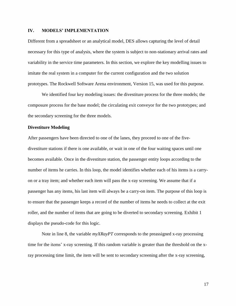
roller, and the number of items that are going to be diverted to secondary screening. Exhibit 1
displays the pseudo-code for this logic.
Note in line 8, the variable myXRayPT corresponds to the preassigned x-ray processing
time for the items’ x-ray screening. If this random variable is greater than the threshold on the x-
ray processing time limit, the item will be sent to secondary screening after the x-ray screening,
18
and the variable storing the number of items to pick up from the exit roller is decreased by one.
In Line 13, one item entity is created every time the passenger goes through the loop.
Exhibit 1. Separate Passengers from Items Logic
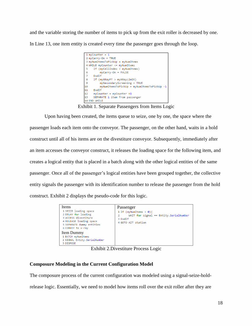
Upon having been created, the items queue to seize, one by one, the space where the
passenger loads each item onto the conveyor. The passenger, on the other hand, waits in a hold
construct until all of his items are on the divestiture conveyor. Subsequently, immediately after
an item accesses the conveyor construct, it releases the loading space for the following item, and
creates a logical entity that is placed in a batch along with the other logical entities of the same
passenger. Once all of the passenger’s logical entities have been grouped together, the collective
entity signals the passenger with its identification number to release the passenger from the hold
construct. Exhibit 2 displays the pseudo-code for this logic.
Items
Item Dummy
Passenger
Exhibit 2.Divestiture Process Logic
Composure Modeling in the Current Configuration Model
The composure process of the current configuration was modeled using a signal-seize-hold-
release logic. Essentially, we need to model how items roll over the exit roller after they are
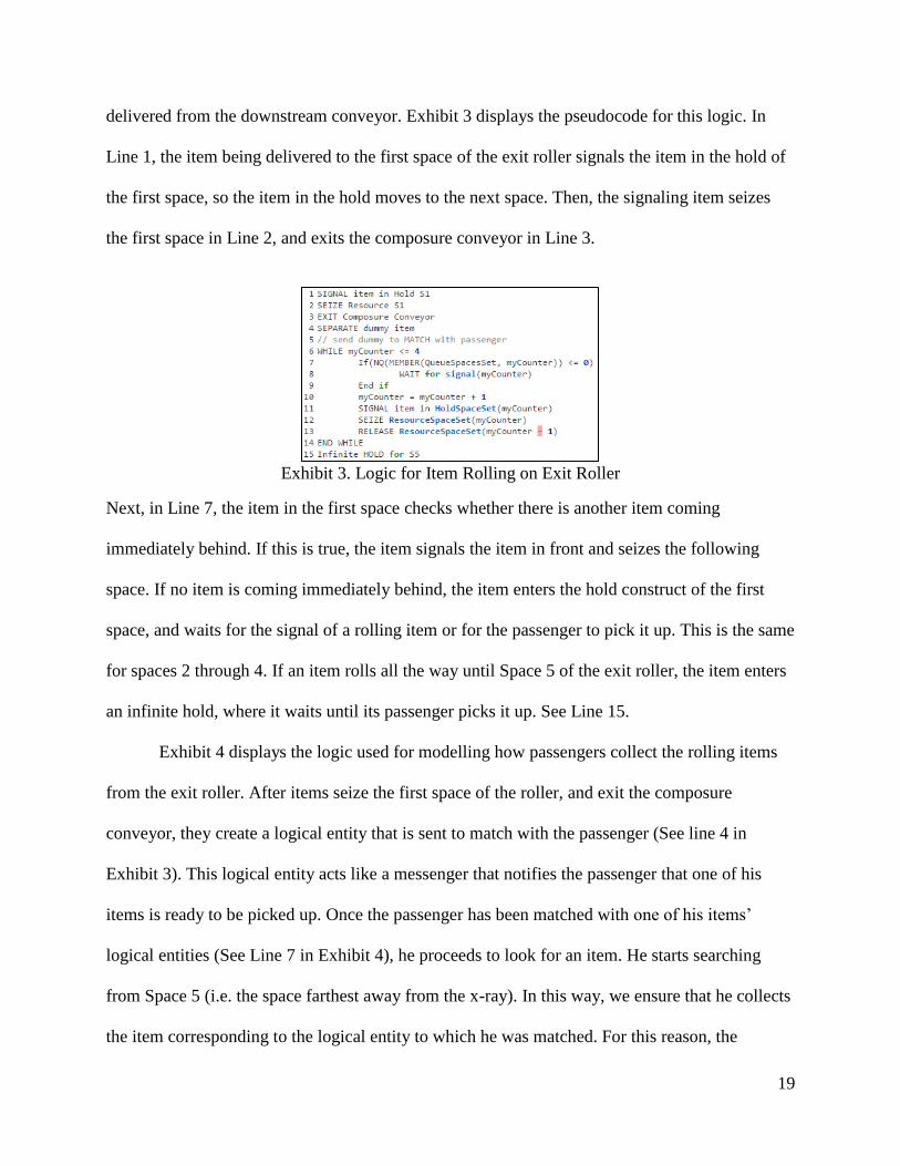
19
delivered from the downstream conveyor. Exhibit 3 displays the pseudocode for this logic. In
Line 1, the item being delivered to the first space of the exit roller signals the item in the hold of
the first space, so the item in the hold moves to the next space. Then, the signaling item seizes
the first space in Line 2, and exits the composure conveyor in Line 3.
Exhibit 3. Logic for Item Rolling on Exit Roller
Next, in Line 7, the item in the first space checks whether there is another item coming
immediately behind. If this is true, the item signals the item in front and seizes the following
space. If no item is coming immediately behind, the item enters the hold construct of the first
space, and waits for the signal of a rolling item or for the passenger to pick it up. This is the same
for spaces 2 through 4. If an item rolls all the way until Space 5 of the exit roller, the item enters
an infinite hold, where it waits until its passenger picks it up. See Line 15.
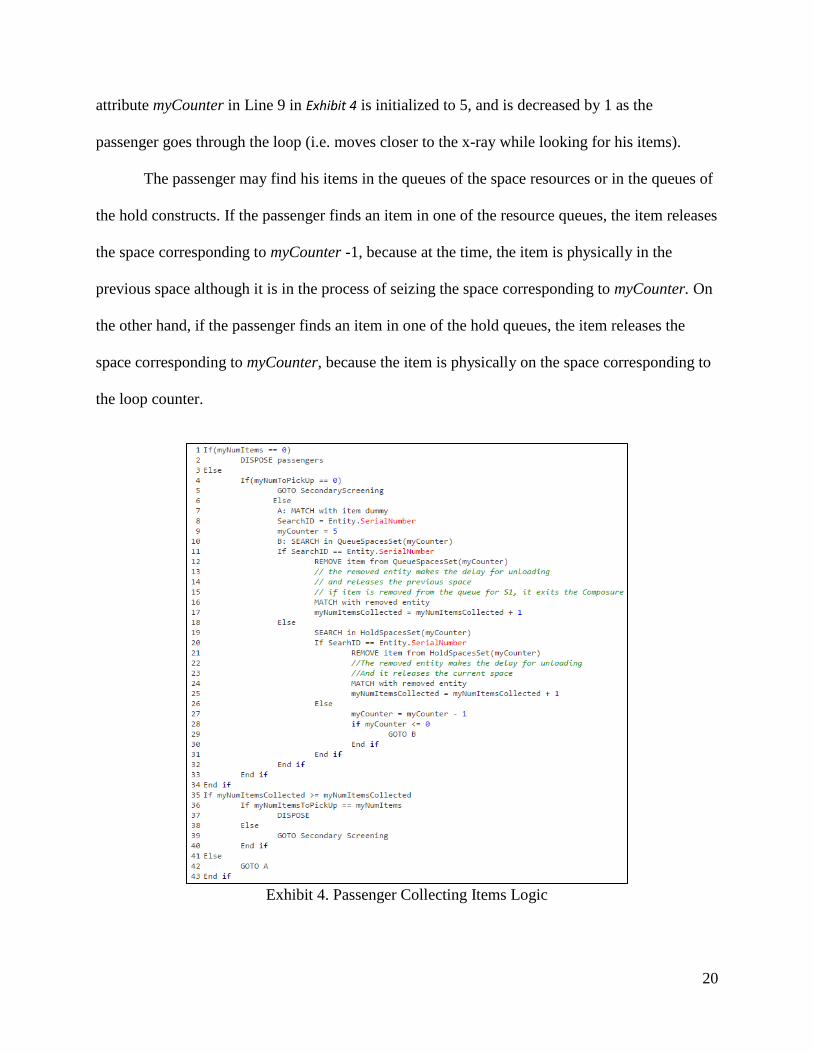
Exhibit 4 displays the logic used for modelling how passengers collect the rolling items
from the exit roller. After items seize the first space of the roller, and exit the composure
conveyor, they create a logical entity that is sent to match with the passenger (See line 4 in
Exhibit 3). This logical entity acts like a messenger that notifies the passenger that one of his
items is ready to be picked up. Once the passenger has been matched with one of his items’
logical entities (See Line 7 in Exhibit 4), he proceeds to look for an item. He starts searching
from Space 5 (i.e. the space farthest away from the x-ray). In this way, we ensure that he collects
the item corresponding to the logical entity to which he was matched. For this reason, the
20
attribute myCounter in Line 9 in Exhibit 4 is initialized to 5, and is decreased by 1 as the
passenger goes through the loop (i.e. moves closer to the x-ray while looking for his items).
The passenger may find his items in the queues of the space resources or in the queues of
the hold constructs. If the passenger finds an item in one of the resource queues, the item releases
the space corresponding to myCounter -1, because at the time, the item is physically in the
previous space although it is in the process of seizing the space corresponding to myCounter. On
the other hand, if the passenger finds an item in one of the hold queues, the item releases the
space corresponding to myCounter, because the item is physically on the space corresponding to
the loop counter.
Exhibit 4. Passenger Collecting Items Logic

21
After the passenger removes an item, he checks whether he needs to collect any other item from
the roller. If this is true, he returns to the match construct to be matched with another logical
entity of his items, and repeats the search process again. Otherwise, he checks whether there is
any of his items at secondary screening. If this is true, he proceeds to secondary screening.
Otherwise, he leaves the checkpoint.
Composure Modeling of the Circulating Conveyor
The composure process for the prototype models follows a different logic than in the current
configuration for the lanes where the exit roller is replaced for a continuously circulating
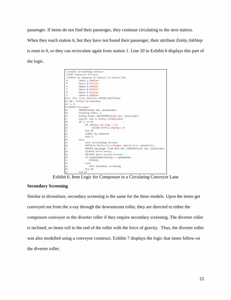
conveyor. Exhibit 5 displays the logic that passengers follow in a circulating conveyor lane.
Exhibit 5. Passenger Logic for Composure in a Circulating Conveyor Lane
After the passenger finds he needs to pick up some items from the circulating conveyor, he
seizes the closest space available around the conveyor. He delays some random time for walking
to the space, and enters a hold construct linked to the space that he seized.
On the other hand, items are delivered to the circulating conveyor by the composure
conveyor. Upon accessing the circulating conveyor, they exit the composure conveyor and
convey by sequence from space 1 to space 6 of the conveyor. In each space, items get assigned
an index associated with the space on which they are. They search the passenger in the hold
queue of the space associated with their index. If they find a passenger with the same serial
number in a particular space, they exit the conveyor and get batched with the other items of the
22
passenger. If items do not find their passenger, they continue circulating to the next station.
When they reach station 6, but they have not found their passenger, their attribute Entity.JobStep
is reset to 0, so they can recirculate again from station 1. Line 20 in Exhibit 6 displays this part of
the logic.
Exhibit 6. Item Logic for Composure in a Circulating Conveyor Lane
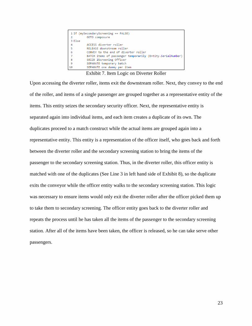
Secondary Screening
Similar to divestiture, secondary screening is the same for the three models. Upon the items get
conveyed out from the x-ray through the downstream roller, they are directed to either the
composure conveyor or the diverter roller if they require secondary screening. The diverter roller
is inclined, so items roll to the end of the roller with the force of gravity. Thus, the diverter roller
was also modelled using a conveyor construct. Exhibit 7 displays the logic that items follow on
the diverter roller.
23
Exhibit 7. Item Logic on Diverter Roller
Upon accessing the diverter roller, items exit the downstream roller. Next, they convey to the end
of the roller, and items of a single passenger are grouped together as a representative entity of the
items. This entity seizes the secondary security officer. Next, the representative entity is
separated again into individual items, and each item creates a duplicate of its own. The
duplicates proceed to a match construct while the actual items are grouped again into a
representative entity. This entity is a representation of the officer itself, who goes back and forth
between the diverter roller and the secondary screening station to bring the items of the
passenger to the secondary screening station. Thus, in the diverter roller, this officer entity is
matched with one of the duplicates (See Line 3 in left hand side of Exhibit 8), so the duplicate
exits the conveyor while the officer entity walks to the secondary screening station. This logic
was necessary to ensure items would only exit the diverter roller after the officer picked them up
to take them to secondary screening. The officer entity goes back to the diverter roller and
repeats the process until he has taken all the items of the passenger to the secondary screening
station. After all of the items have been taken, the officer is released, so he can take serve other
passengers.
24
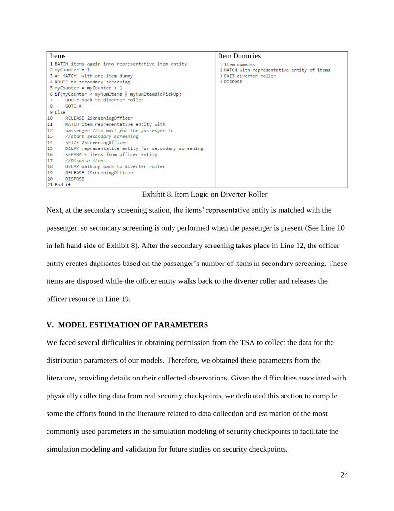
Next, at the secondary screening station, the items’ representative entity is matched with the
passenger, so secondary screening is only performed when the passenger is present (See Line 10
in left hand side of Exhibit 8). After the secondary screening takes place in Line 12, the officer
entity creates duplicates based on the passenger’s number of items in secondary screening. These
items are disposed while the officer entity walks back to the diverter roller and releases the
officer resource in Line 19.
V. MODEL ESTIMATION OF PARAMETERS
We faced several difficulties in obtaining permission from the TSA to collect the data for the
distribution parameters of our models. Therefore, we obtained these parameters from the
literature, providing details on their collected observations. Given the difficulties associated with
physically collecting data from real security checkpoints, we dedicated this section to compile
some the efforts found in the literature related to data collection and estimation of the most
commonly used parameters in the simulation modeling of security checkpoints to facilitate the
simulation modeling and validation for future studies on security checkpoints.
Items Item Dummies
Exhibit 8. Item Logic on Diverter Roller

25
Data Collection on Arrival Patterns
De Barros and Tomber (2007) assert that passenger arrivals to the checkpoint depend on the
flight schedule and the passenger earliness of arrival (EOA) profiles. They claim, a common
simplifying assumption is to use the same EOA regardless of the time of the day although
variation does occur during the day. Passengers flying in the morning tend to arrive much closer
to the departing time than those flying at noon or in the afternoon. They do obtain different EOA
profiles for domestic and international travelers. After extensive collection of data a Seattle-
Tacoma International Airport, they obtained the EOA profiles displayed in Table 1. They
combine these EOA with the airport flight schedule to obtain an arrival schedule for passengers
and luggage’ screening.
Table 1.Earliness of Arrival Profile at Seattle-Tacoma International Airport
In addition, Paul et al. (2009) studied the factors that may affect the passenger flow patterns.
Using an analysis of variance (ANOVA) of a general linear model, they concluded that both day
Time to Departure
Interval Domestic International
0-15 1 0% 0%
15-30 2 2% 0%
30-45 3 2% 1%
45-60 4 6% 4%
60-75 5 13% 13%
80-90 6 22% 21%
90-105 7 24% 23%
105-120 8 19% 19%
120-135 9 10% 11%
135-150 10 2% 5%
150-165 11 0% 2%
165-180 12 0% 1%
180-195 13 0% 0%
195-210 14 0% 0%
210-225 15 0% 0%
225-240 16 0% 0%

26
and time of the day and the interaction between both have a significant effect on the passenger
volume. Figure 4 displays the total passenger volume per day of the week. In addition, their
ANOVA results suggested that four different patterns should be used to generate the passenger
arrivals of a week. These are Monday, Saturday, Sunday and Tuesday through Friday. Figure 5
displays the variation of the passenger volume throughout the day for each four-day pattern.
Figure 4. Passenger Volume per day of the week
Figure 5. Passenger Volume per hour of the day
7,000
7,500
8,000
8,500
9,000
9,500
10,000
Mon Tue Wed Thu Fri Sat Sun
Nu
mb
er o
f P
ass
enge
rs
Total Passenger Volume Per Day
0
20
40
60
80
100
120
Rel
ati
ve N
um
ber
of
Pa
ssen
gers
(%)
Passenger Volume Per Hour of the Day
Monday Satuday Sunday Tue-Fri
27
As Paul et al. (2009) suggest, the highest levels of passenger traffic occur between 5 am and 8
am, and between 4 pm to 6 pm. In addition, Mondays displayed the highest passenger traffic
volumes while Saturdays displayed the lowest. Nonetheless, the authors failed to specify the size
of the airport from which they collected these passenger traffic volumes.
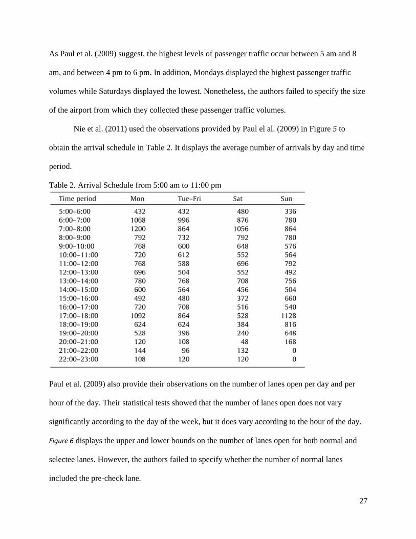
Nie et al. (2011) used the observations provided by Paul el al. (2009) in Figure 5 to
obtain the arrival schedule in Table 2. It displays the average number of arrivals by day and time
period.
Table 2. Arrival Schedule from 5:00 am to 11:00 pm
Paul et al. (2009) also provide their observations on the number of lanes open per day and per
hour of the day. Their statistical tests showed that the number of lanes open does not vary
significantly according to the day of the week, but it does vary according to the hour of the day.
Figure 6 displays the upper and lower bounds on the number of lanes open for both normal and
selectee lanes. However, the authors failed to specify whether the number of normal lanes
included the pre-check lane.

28
Figure 6. Number of Lanes Open per Hour of the Day
De Lange, Samoilovich and Der Rhee also provide their arrival patterns along with the average
number of lanes open for each hour the day. They collected these observations at a large airport
in Western Europe. Figure 7 displays the graph summarizing their observations.
Figure 7. Arrival Patterns and Lane Idle Capoacity at a Larger Airport in Western Europe
The distribution for the walking velocity of the passengers and the security officers was also
obtained from literature. We used a triangular distribution with parameters 2.93, 4.4 and 5.86
feet per second (Hobbs, Rossetti and Faas, 2006).
0
1
2
3
4
5
6
5:00 6:00 7:00 8:00 9:00 10:00 11:00 12:00 13:00 14:00 15:00 16:00 17:00 18:00 19:00 20:00 21:00 22:00
Nu
mb
er o
f La
nes
Op
en
Number of Lanes Open (Normal and Selectee)
Upper Bound - No of Open Normal Lanes Lower Bound - No of Open Normal Lanes
Upper Bound - No of Open Selectee Lanes Lower Bound - No of Open Selectee Lanes
29
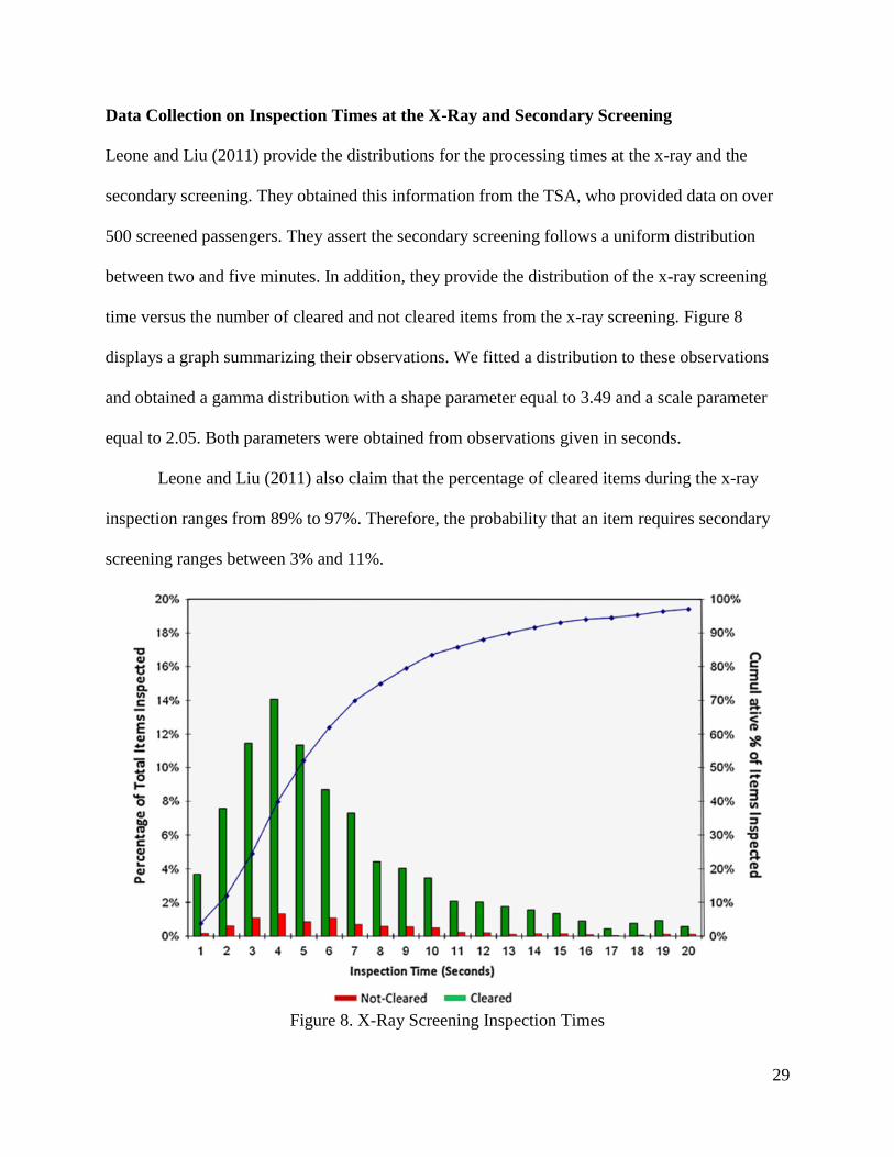
Data Collection on Inspection Times at the X-Ray and Secondary Screening
Leone and Liu (2011) provide the distributions for the processing times at the x-ray and the
secondary screening. They obtained this information from the TSA, who provided data on over
500 screened passengers. They assert the secondary screening follows a uniform distribution
between two and five minutes. In addition, they provide the distribution of the x-ray screening
time versus the number of cleared and not cleared items from the x-ray screening. Figure 8
displays a graph summarizing their observations. We fitted a distribution to these observations
and obtained a gamma distribution with a shape parameter equal to 3.49 and a scale parameter
equal to 2.05. Both parameters were obtained from observations given in seconds.
Leone and Liu (2011) also claim that the percentage of cleared items during the x-ray
inspection ranges from 89% to 97%. Therefore, the probability that an item requires secondary
screening ranges between 3% and 11%.
Figure 8. X-Ray Screening Inspection Times
30
Nie et al. (2011) also provide details on their distributions for the x-ray and secondary screening
inspections. They use a triangular distribution with parameters 10, 12 and 14 seconds for the x-
ray inspection of a selectee lane, and parameters of 8, 10, and 12 seconds for the x-ray inspection
of a non-selectee lane. For the manual inspection at secondary screening, they fit a gamma
distribution with shape parameter of 2 minutes and scale parameter of 2.05 minutes.
For our models, we used the gamma distribution we obtained from Leone and Liu’s
observations for the x-ray inspection. In addition, we used Nie et al.’s gamma distribution on the
inspection time for secondary screening, because it allowed using the coefficient of variation to
try different levels of the mean for the experimentation section.
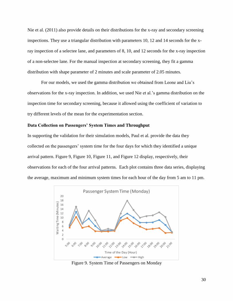
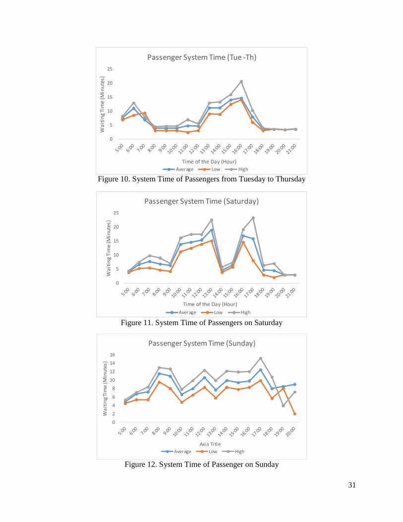
Data Collection on Passengers’ System Times and Throughput
In supporting the validation for their simulation models, Paul et al. provide the data they
collected on the passengers’ system time for the four days for which they identified a unique
arrival pattern. Figure 9, Figure 10, Figure 11, and Figure 12 display, respectively, their
observations for each of the four arrival patterns. Each plot contains three data series, displaying
the average, maximum and minimum system times for each hour of the day from 5 am to 11 pm.
Figure 9. System Time of Passengers on Monday
0
2
4
6
8
10
12
14
16
18
20
Wa
itin
g Ti
me
(Min
ute
s)
Time of the Day (Hour)
Passenger System Time (Monday)
Average Low High
31
Figure 10. System Time of Passengers from Tuesday to Thursday
Figure 11. System Time of Passengers on Saturday
Figure 12. System Time of Passenger on Sunday
0
5
10
15
20
25
Wa
itin
g Ti
me
(Min
ute
s)
Time of the Day (Hour)
Passenger System Time (Tue -Th)
Average Low High
0
5
10
15
20
25
Wa
itin
g Ti
me
(Min
ute
s)
Time of the Day (Hour)
Passenger System Time (Saturday)
Average Low High
0
2
4
6
8
10
12
14
16
Wa
itin
g Ti
me
(Min
ute
s)
Axis Title
Passenger System Time (Sunday)
Average Low High
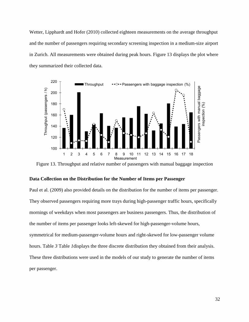
32
Wetter, Lipphardt and Hofer (2010) collected eighteen measurements on the average throughput
and the number of passengers requiring secondary screening inspection in a medium-size airport
in Zurich. All measurements were obtained during peak hours. Figure 13 displays the plot where
they summarized their collected data.
Figure 13. Throughput and relative number of passengers with manual baggage inspection
Data Collection on the Distribution for the Number of Items per Passenger
Paul et al. (2009) also provided details on the distribution for the number of items per passenger.
They observed passengers requiring more trays during high-passenger traffic hours, specifically
mornings of weekdays when most passengers are business passengers. Thus, the distribution of
the number of items per passenger looks left-skewed for high-passenger-volume hours,
symmetrical for medium-passenger-volume hours and right-skewed for low-passenger volume
hours. Table 3 Table 1displays the three discrete distribution they obtained from their analysis.
These three distributions were used in the models of our study to generate the number of items
per passenger.
33
Table 3. Distribution of Items per Passenger (Paul et al, 2009)
Items per Passenger
Passenger Volume 0 Items 1 Item 2 Items 3 Items 4 Items 5 Items
High 0 5 10 20 40 25
Medium 2.5 10 20 40 20 7.5
Low 2.5 25 35 20 12.5 5
Dorton and Liu (2016) also provide details on their distribution for the number of items per
passenger. Different from Paul et al. (2009), they only provide a single discrete distribution for a
general traffic volume of passengers, and they adjust their distribution such as every passenger
has at least one item. Table 4 displays the probability mass function for the distribution they used
in their simulation model.
Table 4. Distribution of Items per Passenger (Dorton and Liu, 2016)
Items per Passenger
# of Items 1 2 3 4 5
PMF 0.03 0.36 0.44 0.16 0.01
Four our models, we used the distributions from Paul et. al, because their parameters are specific
for the traffic volume of passengers.
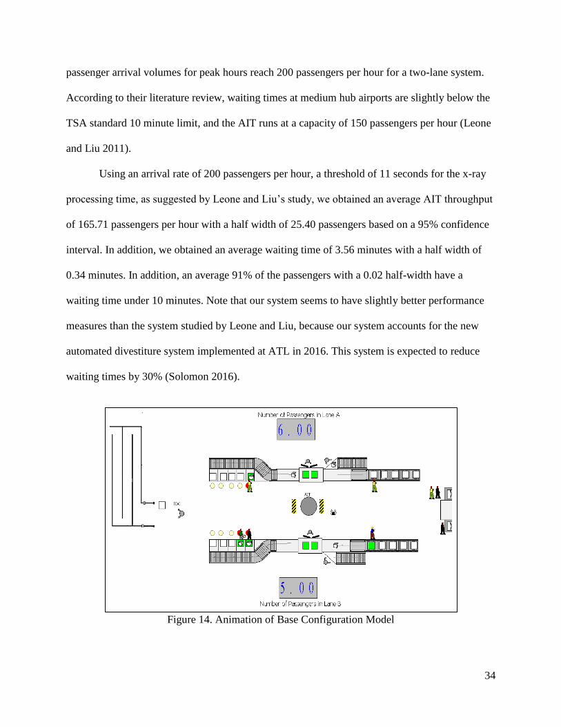
VI. MODELS’ VALIDATION AND VERIFICATION
The model verification consisted of ensuring that the key modeling issues worked exactly as
intended. We accomplished this by carefully animating the key modeling issues in the three
models while debugging what looked unusual in the animation. Figure 14, Error! Reference
source not found., and Figure 16 display a picture for the base configuration and the two
solution prototypes.
The models’ validation consisted of making sure that the model accurately represented
the real system. According to Leone and Liu’s airport classification, the volume of passengers
taken into account for this study corresponds to the volume of a medium hub airport where
34
passenger arrival volumes for peak hours reach 200 passengers per hour for a two-lane system.
According to their literature review, waiting times at medium hub airports are slightly below the
TSA standard 10 minute limit, and the AIT runs at a capacity of 150 passengers per hour (Leone
and Liu 2011).
Using an arrival rate of 200 passengers per hour, a threshold of 11 seconds for the x-ray
processing time, as suggested by Leone and Liu’s study, we obtained an average AIT throughput
of 165.71 passengers per hour with a half width of 25.40 passengers based on a 95% confidence
interval. In addition, we obtained an average waiting time of 3.56 minutes with a half width of
0.34 minutes. In addition, an average 91% of the passengers with a 0.02 half-width have a
waiting time under 10 minutes. Note that our system seems to have slightly better performance
measures than the system studied by Leone and Liu, because our system accounts for the new
automated divestiture system implemented at ATL in 2016. This system is expected to reduce
waiting times by 30% (Solomon 2016).
Figure 14. Animation of Base Configuration Model

35
Figure 15. Animation of the Prototype 1 Model
Figure 16. Animation of Second Prototype Model
VII. EXPERIMENTATION AND RESULTS
The performance of the circulating conveyor highly depends on the amount of items being
delivered to the conveyor. If the flow level of items being delivered from the x-ray station is low,
the circulating conveyor could be unnecessary. In addition, as Leone and Liu (2011) concluded
in their study, limiting the x-ray processing time of every item while routing to secondary
screening any item requiring additional screening time, could significantly reduce the waiting
36
time of passengers. Moreover, the circulating conveyor is expected to accelerate the item flow by
providing more space and clearing the roller’s space faster. Thus, the first stage of the
experimentation consisted of investigating the effect of the circulating conveyor on the optimal
x-ray processing time limit, proposed by Leone and Liu’s study. First, we verified Leone and
Liu’s findings using the simulation model for the base configuration. Then, we observed how
the threshold changed with the models for the first and second prototypes. Additional sensitivity
analysis was performed using the coefficient of variation of the secondary screening distribution.
In addition, given that a lane having the circulating conveyor is expected to process
passengers faster than a lane featuring a traditional exit roller, using the model for the first
prototype, we explored the possibility of directing passengers likely to take longer, to the lane
best suited for their processing. Because passengers who carry more items may require additional
time for processing, we expect the passenger’s processing time to be positively correlated with
the quantity of items carried by the passengers. Consequently, we used simulation optimization
to find the threshold on the maximum number of items that a passenger can have to be able to
process at the lane featuring a traditional layout. Passengers carrying a number of items above
this threshold will be directed to the lane featuring the circulating conveyor in order to
compensate for the additional time that these passengers take.
Lastly, we explored the possibility of replacing two traditional lanes with one circulating
conveyor lane. We conduct a sensitivity analysis on the arrival rate of passengers in order to
determine the arrival rates under which the performance of one circulating conveyor lane is
comparable to the performance of a traditional two-lane system. In the following sections, we
will examine each part of the experimentation in detail.
37
Threshold on the X-Ray Processing Time Limit
This portion of the experimentation consisted of finding the x-ray processing time limit that
results in the minimum average system time, using the simulation model for the base
configuration as well as the models for the first and second prototypes.
Leone and Liu (2011) performed their experiments on a system operating at capacity.
According to their proposal, their system was unable to complete the processing of all the 200
incoming passengers without their suggested recommendation. Consequently, we performed this
stage of the experimentation with a system at capacity. As we observed during the validation
section, our models, featuring the new divestiture system, were able to process 200 pph,
completely with 90% of the passengers being processed within 10 minutes. Therefore, we
decided to increment the mean arrival rate of the exponential distribution of our models to 300
pph for this stage of the experimentation in order to have a system operating at capacity.
First, an exploratory analysis was performed to investigate the relationship between the
x-ray processing time limit and the system time in the base model. Next, a polynomial regression
analysis was conducted to find the limit resulting in the minimum system time. Lastly, a
sensitivity analysis was performed by varying the parameters of the secondary screening
distribution, and testing how the optimum limit would change with the prototype models.
Exploratory Analysis
For an initial screening of the two variables, 176 scenarios of 15 replications each were
performed, using the model for the base configuration. Each scenario differed in the x-ray
processing time limit parameter, which ranged between 7.5 and 25 seconds among the 176
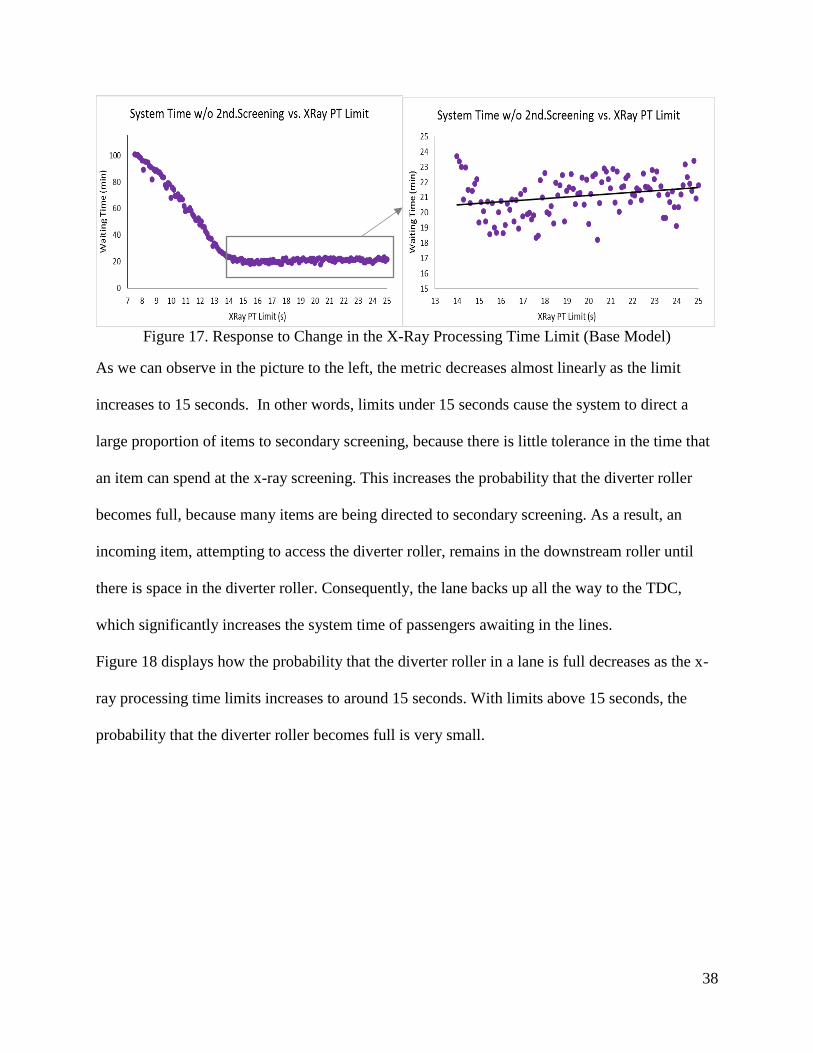
scenarios. Figure 17 displays the results for this initial screening.
38
Figure 17. Response to Change in the X-Ray Processing Time Limit (Base Model)
As we can observe in the picture to the left, the metric decreases almost linearly as the limit
increases to 15 seconds. In other words, limits under 15 seconds cause the system to direct a
large proportion of items to secondary screening, because there is little tolerance in the time that
an item can spend at the x-ray screening. This increases the probability that the diverter roller
becomes full, because many items are being directed to secondary screening. As a result, an
incoming item, attempting to access the diverter roller, remains in the downstream roller until
there is space in the diverter roller. Consequently, the lane backs up all the way to the TDC,
which significantly increases the system time of passengers awaiting in the lines.
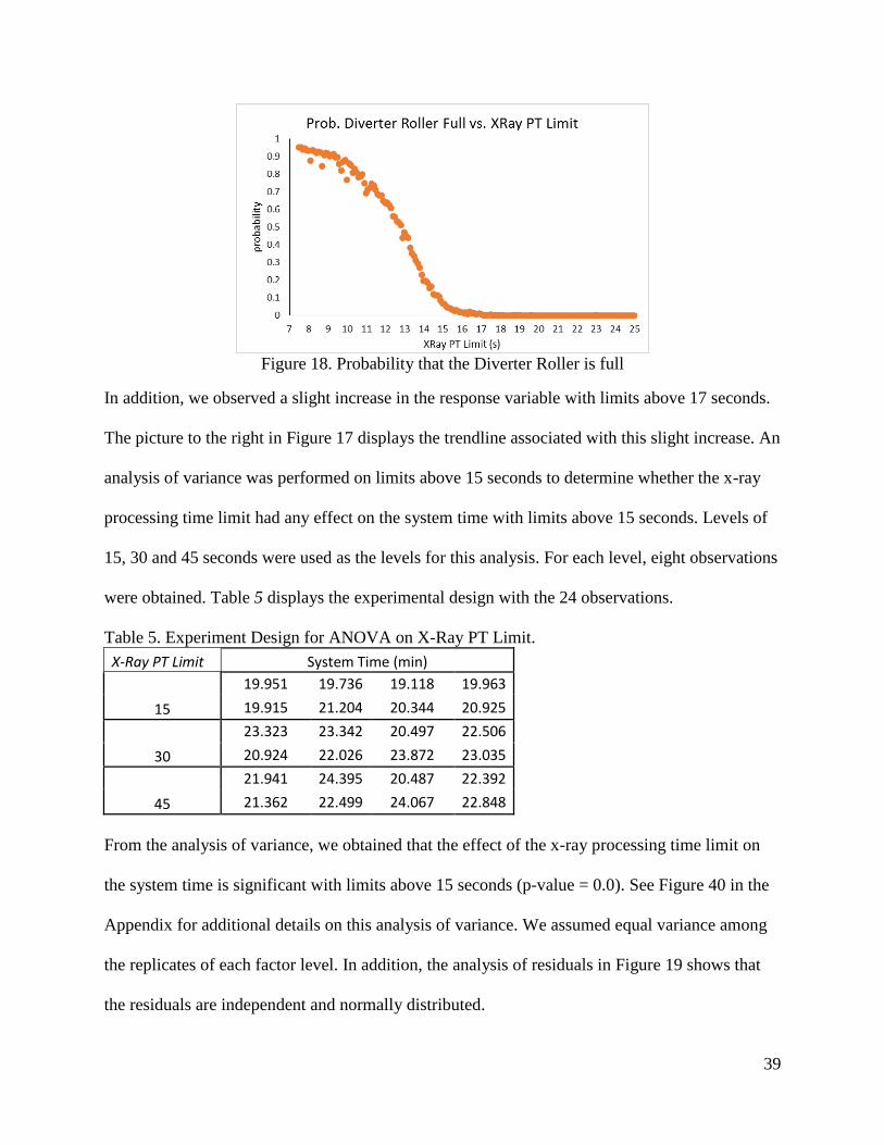
Figure 18 displays how the probability that the diverter roller in a lane is full decreases as the x-
ray processing time limits increases to around 15 seconds. With limits above 15 seconds, the
probability that the diverter roller becomes full is very small.
39
Figure 18. Probability that the Diverter Roller is full
In addition, we observed a slight increase in the response variable with limits above 17 seconds.
The picture to the right in Figure 17 displays the trendline associated with this slight increase. An
analysis of variance was performed on limits above 15 seconds to determine whether the x-ray
processing time limit had any effect on the system time with limits above 15 seconds. Levels of
15, 30 and 45 seconds were used as the levels for this analysis. For each level, eight observations
were obtained. Table 5 displays the experimental design with the 24 observations.
Table 5. Experiment Design for ANOVA on X-Ray PT Limit.
X-Ray PT Limit System Time (min)
15
19.951 19.736 19.118 19.963
19.915 21.204 20.344 20.925
30
23.323 23.342 20.497 22.506
20.924 22.026 23.872 23.035
45
21.941 24.395 20.487 22.392
21.362 22.499 24.067 22.848
From the analysis of variance, we obtained that the effect of the x-ray processing time limit on
the system time is significant with limits above 15 seconds (p-value = 0.0). See Figure 40 in the
Appendix for additional details on this analysis of variance. We assumed equal variance among
the replicates of each factor level. In addition, the analysis of residuals in Figure 19 shows that
the residuals are independent and normally distributed.
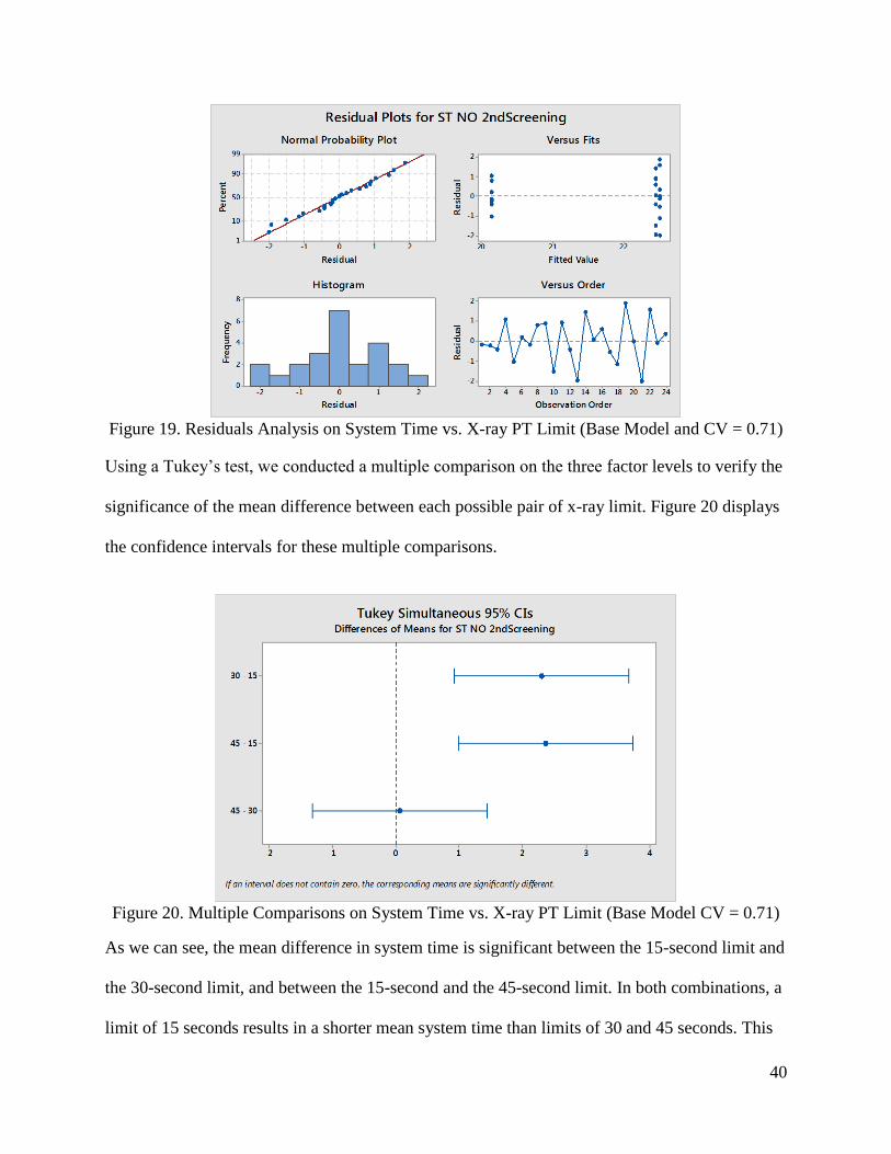
40
Figure 19. Residuals Analysis on System Time vs. X-ray PT Limit (Base Model and CV = 0.71)
Using a Tukey’s test, we conducted a multiple comparison on the three factor levels to verify the
significance of the mean difference between each possible pair of x-ray limit. Figure 20 displays
the confidence intervals for these multiple comparisons.
Figure 20. Multiple Comparisons on System Time vs. X-ray PT Limit (Base Model CV = 0.71)
As we can see, the mean difference in system time is significant between the 15-second limit and
the 30-second limit, and between the 15-second and the 45-second limit. In both combinations, a
limit of 15 seconds results in a shorter mean system time than limits of 30 and 45 seconds. This
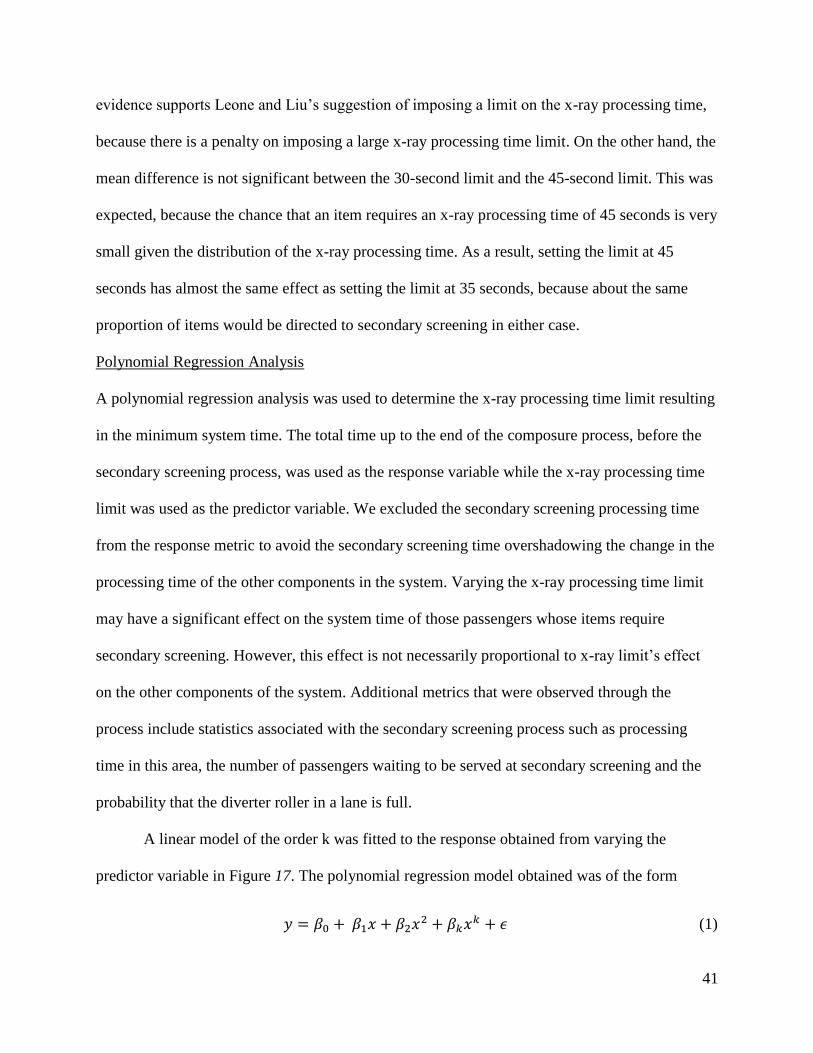
41
evidence supports Leone and Liu’s suggestion of imposing a limit on the x-ray processing time,
because there is a penalty on imposing a large x-ray processing time limit. On the other hand, the
mean difference is not significant between the 30-second limit and the 45-second limit. This was
expected, because the chance that an item requires an x-ray processing time of 45 seconds is very
small given the distribution of the x-ray processing time. As a result, setting the limit at 45
seconds has almost the same effect as setting the limit at 35 seconds, because about the same
proportion of items would be directed to secondary screening in either case.
Polynomial Regression Analysis
A polynomial regression analysis was used to determine the x-ray processing time limit resulting
in the minimum system time. The total time up to the end of the composure process, before the
secondary screening process, was used as the response variable while the x-ray processing time
limit was used as the predictor variable. We excluded the secondary screening processing time
from the response metric to avoid the secondary screening time overshadowing the change in the
processing time of the other components in the system. Varying the x-ray processing time limit
may have a significant effect on the system time of those passengers whose items require
secondary screening. However, this effect is not necessarily proportional to x-ray limit’s effect
on the other components of the system. Additional metrics that were observed through the
process include statistics associated with the secondary screening process such as processing
time in this area, the number of passengers waiting to be served at secondary screening and the
probability that the diverter roller in a lane is full.
A linear model of the order k was fitted to the response obtained from varying the
predictor variable in Figure 17. The polynomial regression model obtained was of the form
𝑦 = 𝛽0 + 𝛽1𝑥 + 𝛽2𝑥2 + 𝛽𝑘𝑥𝑘 + 𝜖 (1)
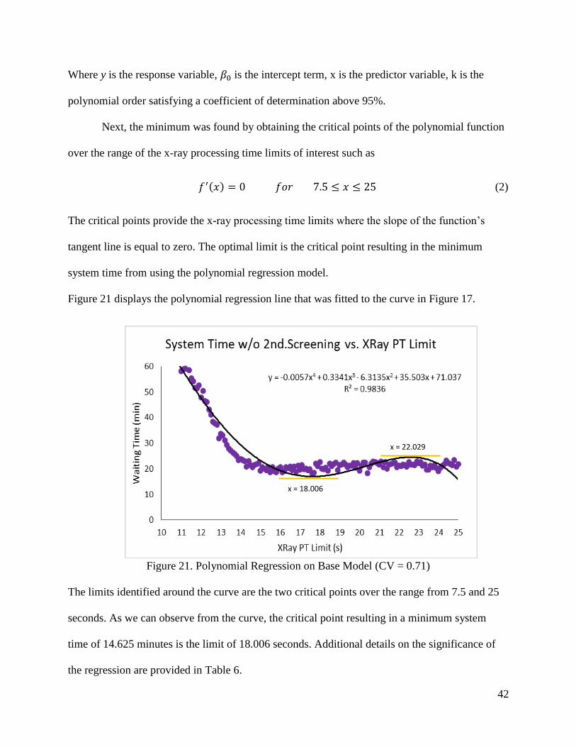
42
Where y is the response variable, 𝛽0 is the intercept term, x is the predictor variable, k is the
polynomial order satisfying a coefficient of determination above 95%.
Next, the minimum was found by obtaining the critical points of the polynomial function
over the range of the x-ray processing time limits of interest such as
𝑓′(𝑥) = 0 𝑓𝑜𝑟 7.5 ≤ 𝑥 ≤ 25 (2)
The critical points provide the x-ray processing time limits where the slope of the function’s
tangent line is equal to zero. The optimal limit is the critical point resulting in the minimum
system time from using the polynomial regression model.
Figure 21 displays the polynomial regression line that was fitted to the curve in Figure 17.
Figure 21. Polynomial Regression on Base Model (CV = 0.71)
The limits identified around the curve are the two critical points over the range from 7.5 and 25
seconds. As we can observe from the curve, the critical point resulting in a minimum system
time of 14.625 minutes is the limit of 18.006 seconds. Additional details on the significance of
the regression are provided in Table 6.
x = 22.029
x = 18.006
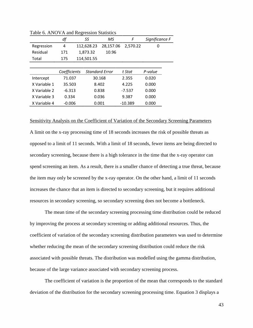
43
Table 6. ANOVA and Regression Statistics df SS MS F Significance F
Regression 4 112,628.23 28,157.06 2,570.22 0
Residual 171 1,873.32 10.96 Total 175 114,501.55
Coefficients Standard Error t Stat P-value
Intercept 71.037 30.168 2.355 0.020
X Variable 1 35.503 8.402 4.225 0.000
X Variable 2 -6.313 0.838 -7.537 0.000
X Variable 3 0.334 0.036 9.387 0.000
X Variable 4 -0.006 0.001 -10.389 0.000
Sensitivity Analysis on the Coefficient of Variation of the Secondary Screening Parameters
A limit on the x-ray processing time of 18 seconds increases the risk of possible threats as
opposed to a limit of 11 seconds. With a limit of 18 seconds, fewer items are being directed to
secondary screening, because there is a high tolerance in the time that the x-ray operator can
spend screening an item. As a result, there is a smaller chance of detecting a true threat, because
the item may only be screened by the x-ray operator. On the other hand, a limit of 11 seconds
increases the chance that an item is directed to secondary screening, but it requires additional
resources in secondary screening, so secondary screening does not become a bottleneck.
The mean time of the secondary screening processing time distribution could be reduced
by improving the process at secondary screening or adding additional resources. Thus, the
coefficient of variation of the secondary screening distribution parameters was used to determine
whether reducing the mean of the secondary screening distribution could reduce the risk
associated with possible threats. The distribution was modelled using the gamma distribution,
because of the large variance associated with secondary screening process.
The coefficient of variation is the proportion of the mean that corresponds to the standard
deviation of the distribution for the secondary screening processing time. Equation 3 displays a
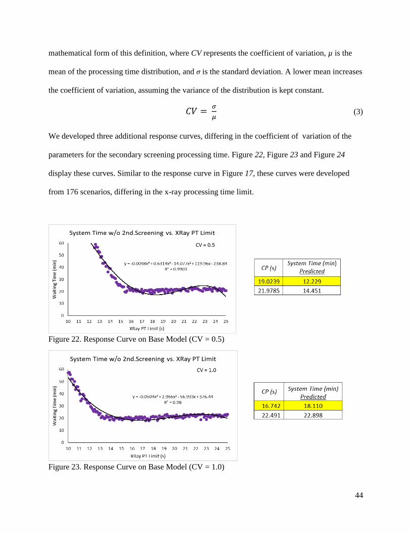
44
mathematical form of this definition, where CV represents the coefficient of variation, µ is the
mean of the processing time distribution, and σ is the standard deviation. A lower mean increases
the coefficient of variation, assuming the variance of the distribution is kept constant.
𝐶𝑉 = 𝜎
𝜇 (3)
We developed three additional response curves, differing in the coefficient of variation of the
parameters for the secondary screening processing time. Figure 22, Figure 23 and Figure 24
display these curves. Similar to the response curve in Figure 17, these curves were developed
from 176 scenarios, differing in the x-ray processing time limit.
Figure 22. Response Curve on Base Model (CV = 0.5)
Figure 23. Response Curve on Base Model (CV = 1.0)
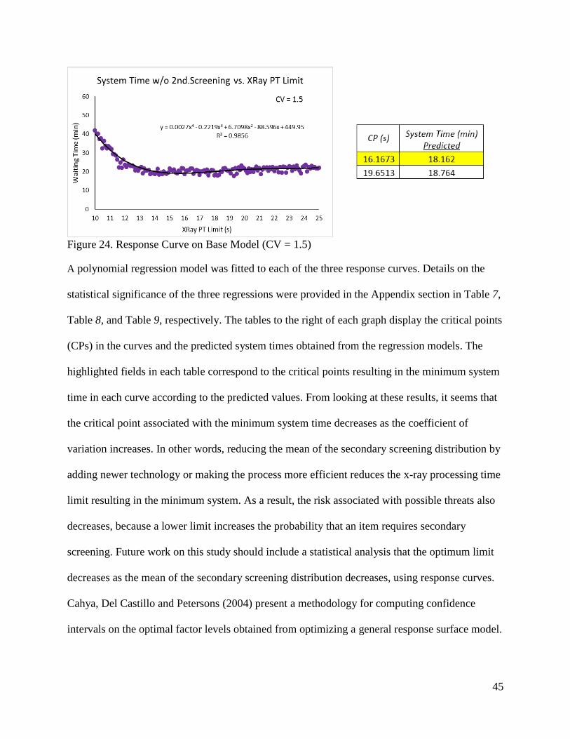
45
Figure 24. Response Curve on Base Model (CV = 1.5)
A polynomial regression model was fitted to each of the three response curves. Details on the
statistical significance of the three regressions were provided in the Appendix section in Table 7,
Table 8, and Table 9, respectively. The tables to the right of each graph display the critical points
(CPs) in the curves and the predicted system times obtained from the regression models. The
highlighted fields in each table correspond to the critical points resulting in the minimum system
time in each curve according to the predicted values. From looking at these results, it seems that
the critical point associated with the minimum system time decreases as the coefficient of
variation increases. In other words, reducing the mean of the secondary screening distribution by
adding newer technology or making the process more efficient reduces the x-ray processing time
limit resulting in the minimum system. As a result, the risk associated with possible threats also
decreases, because a lower limit increases the probability that an item requires secondary
screening. Future work on this study should include a statistical analysis that the optimum limit
decreases as the mean of the secondary screening distribution decreases, using response curves.
Cahya, Del Castillo and Petersons (2004) present a methodology for computing confidence
intervals on the optimal factor levels obtained from optimizing a general response surface model.
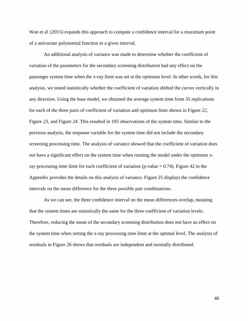
46
Wan et al. (2015) expands this approach to compute a confidence interval for a maximum point
of a univariate polynomial function in a given interval.
An additional analysis of variance was made to determine whether the coefficient of
variation of the parameters for the secondary screening distribution had any effect on the
passenger system time when the x-ray limit was set at the optimum level. In other words, for this
analysis, we tested statistically whether the coefficient of variation shifted the curves vertically in
any direction. Using the base model, we obtained the average system time from 35 replications
for each of the three pairs of coefficient of variation and optimum limit shown in Figure 22,
Figure 23, and Figure 24. This resulted in 105 observations of the system time. Similar to the
previous analysis, the response variable for the system time did not include the secondary
screening processing time. The analysis of variance showed that the coefficient of variation does
not have a significant effect on the system time when running the model under the optimum x-
ray processing time limit for each coefficient of variation (p-value = 0.74). Figure 42 in the
Appendix provides the details on this analysis of variance. Figure 25 displays the confidence
intervals on the mean difference for the three possible pair combinations.
As we can see, the three confidence interval on the mean differences overlap, meaning
that the system times are statistically the same for the three coefficient of variation levels.
Therefore, reducing the mean of the secondary screening distribution does not have an effect on
the system time when setting the x-ray processing time limit at the optimal level. The analysis of
residuals in Figure 26 shows that residuals are independent and normally distributed.
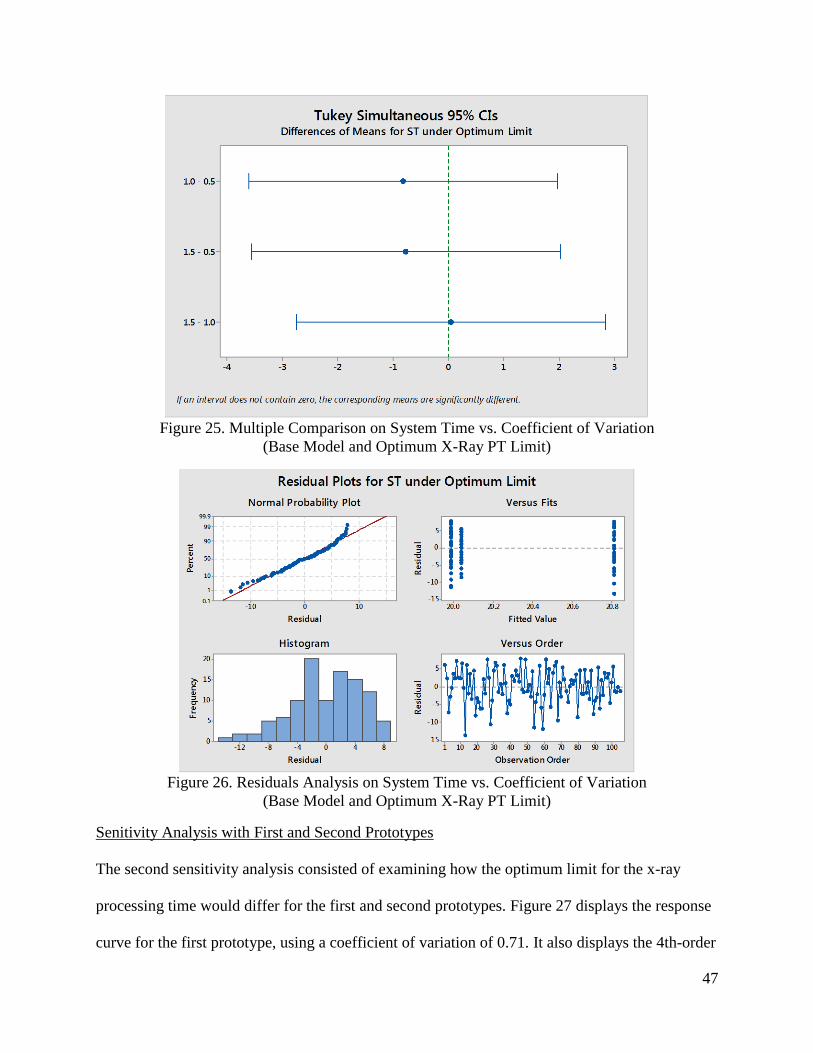
47
Figure 25. Multiple Comparison on System Time vs. Coefficient of Variation
(Base Model and Optimum X-Ray PT Limit)
Figure 26. Residuals Analysis on System Time vs. Coefficient of Variation
(Base Model and Optimum X-Ray PT Limit)
Senitivity Analysis with First and Second Prototypes
The second sensitivity analysis consisted of examining how the optimum limit for the x-ray
processing time would differ for the first and second prototypes. Figure 27 displays the response
curve for the first prototype, using a coefficient of variation of 0.71. It also displays the 4th-order
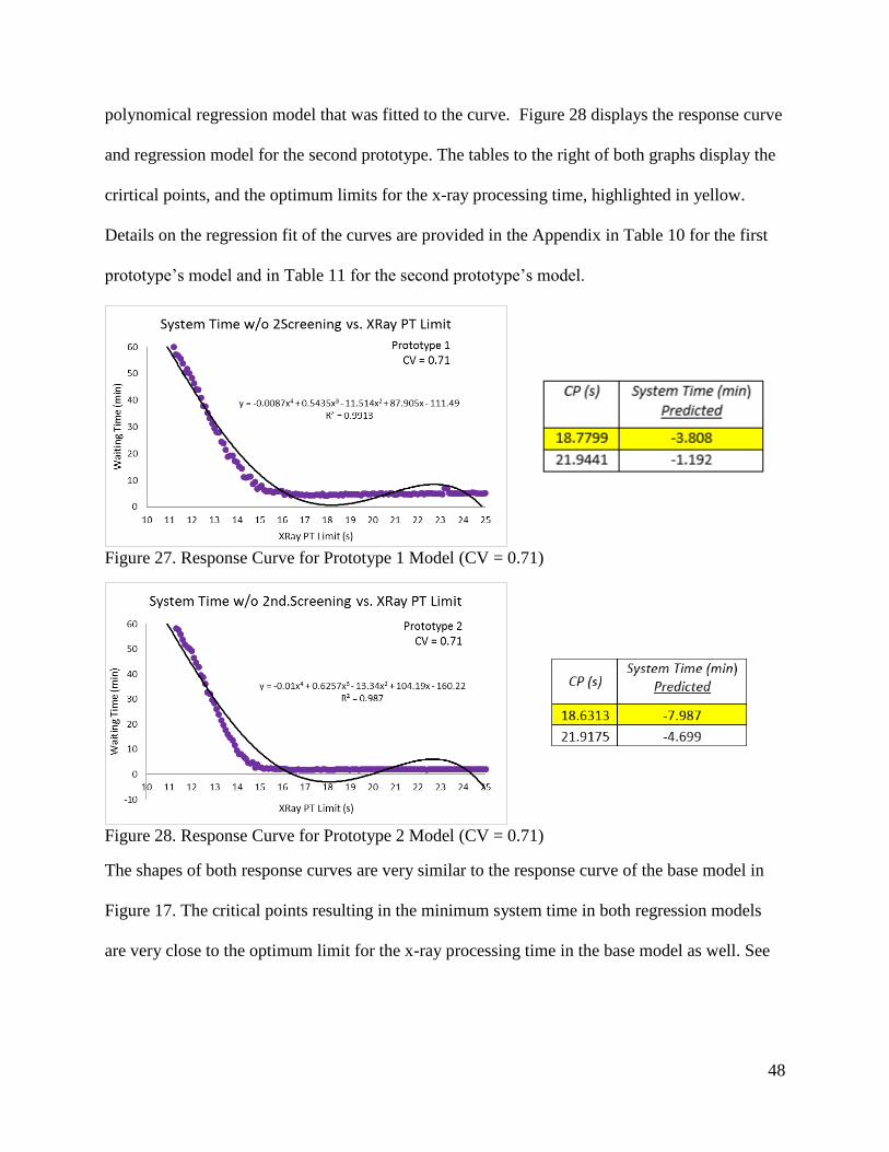
48
polynomical regression model that was fitted to the curve. Figure 28 displays the response curve
and regression model for the second prototype. The tables to the right of both graphs display the
crirtical points, and the optimum limits for the x-ray processing time, highlighted in yellow.
Details on the regression fit of the curves are provided in the Appendix in Table 10 for the first
prototype’s model and in Table 11 for the second prototype’s model.
Figure 27. Response Curve for Prototype 1 Model (CV = 0.71)
Figure 28. Response Curve for Prototype 2 Model (CV = 0.71)
The shapes of both response curves are very similar to the response curve of the base model in
Figure 17. The critical points resulting in the minimum system time in both regression models
are very close to the optimum limit for the x-ray processing time in the base model as well. See
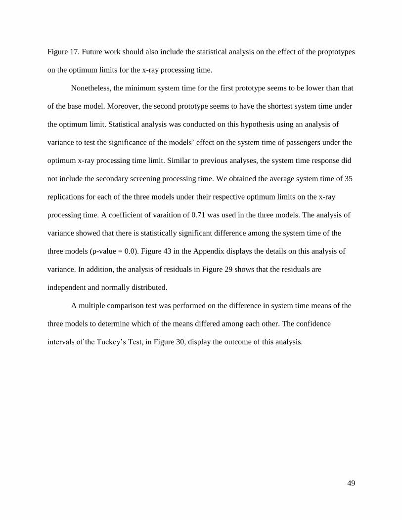
49
Figure 17. Future work should also include the statistical analysis on the effect of the proptotypes
on the optimum limits for the x-ray processing time.
Nonetheless, the minimum system time for the first prototype seems to be lower than that
of the base model. Moreover, the second prototype seems to have the shortest system time under
the optimum limit. Statistical analysis was conducted on this hypothesis using an analysis of
variance to test the significance of the models’ effect on the system time of passengers under the
optimum x-ray processing time limit. Similar to previous analyses, the system time response did
not include the secondary screening processing time. We obtained the average system time of 35
replications for each of the three models under their respective optimum limits on the x-ray
processing time. A coefficient of varaition of 0.71 was used in the three models. The analysis of
variance showed that there is statistically significant difference among the system time of the
three models (p-value = 0.0). Figure 43 in the Appendix displays the details on this analysis of
variance. In addition, the analysis of residuals in Figure 29 shows that the residuals are
independent and normally distributed.
A multiple comparison test was performed on the difference in system time means of the
three models to determine which of the means differed among each other. The confidence
intervals of the Tuckey’s Test, in Figure 30, display the outcome of this analysis.
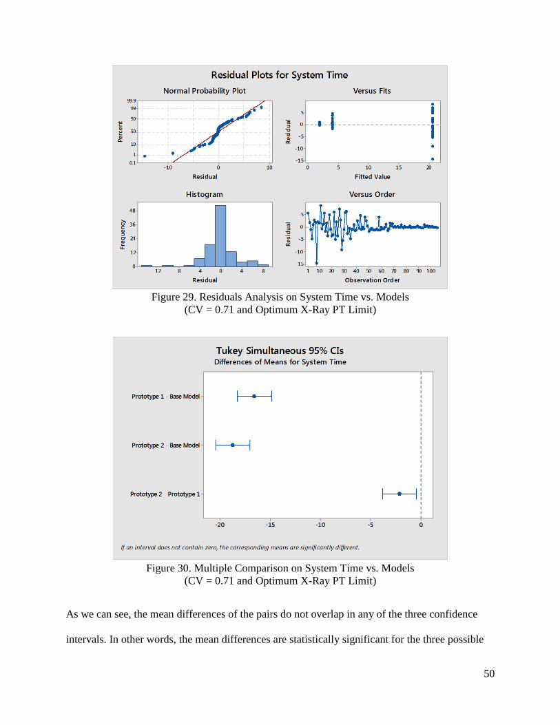
50
Figure 29. Residuals Analysis on System Time vs. Models
(CV = 0.71 and Optimum X-Ray PT Limit)
Figure 30. Multiple Comparison on System Time vs. Models
(CV = 0.71 and Optimum X-Ray PT Limit)
As we can see, the mean differences of the pairs do not overlap in any of the three confidence
intervals. In other words, the mean differences are statistically significant for the three possible
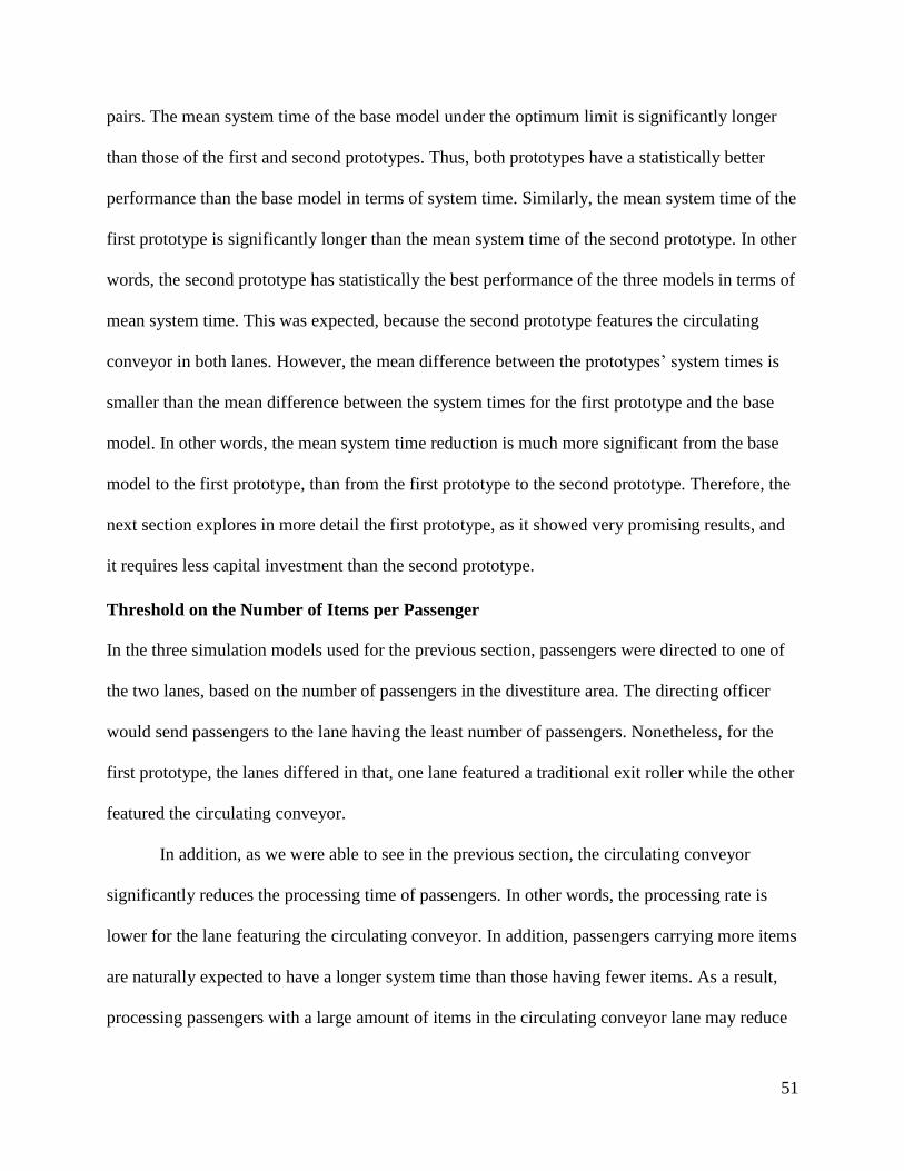
51
pairs. The mean system time of the base model under the optimum limit is significantly longer
than those of the first and second prototypes. Thus, both prototypes have a statistically better
performance than the base model in terms of system time. Similarly, the mean system time of the
first prototype is significantly longer than the mean system time of the second prototype. In other
words, the second prototype has statistically the best performance of the three models in terms of
mean system time. This was expected, because the second prototype features the circulating
conveyor in both lanes. However, the mean difference between the prototypes’ system times is
smaller than the mean difference between the system times for the first prototype and the base
model. In other words, the mean system time reduction is much more significant from the base
model to the first prototype, than from the first prototype to the second prototype. Therefore, the
next section explores in more detail the first prototype, as it showed very promising results, and
it requires less capital investment than the second prototype.
Threshold on the Number of Items per Passenger
In the three simulation models used for the previous section, passengers were directed to one of
the two lanes, based on the number of passengers in the divestiture area. The directing officer
would send passengers to the lane having the least number of passengers. Nonetheless, for the
first prototype, the lanes differed in that, one lane featured a traditional exit roller while the other
featured the circulating conveyor.
In addition, as we were able to see in the previous section, the circulating conveyor
significantly reduces the processing time of passengers. In other words, the processing rate is
lower for the lane featuring the circulating conveyor. In addition, passengers carrying more items
are naturally expected to have a longer system time than those having fewer items. As a result,
processing passengers with a large amount of items in the circulating conveyor lane may reduce
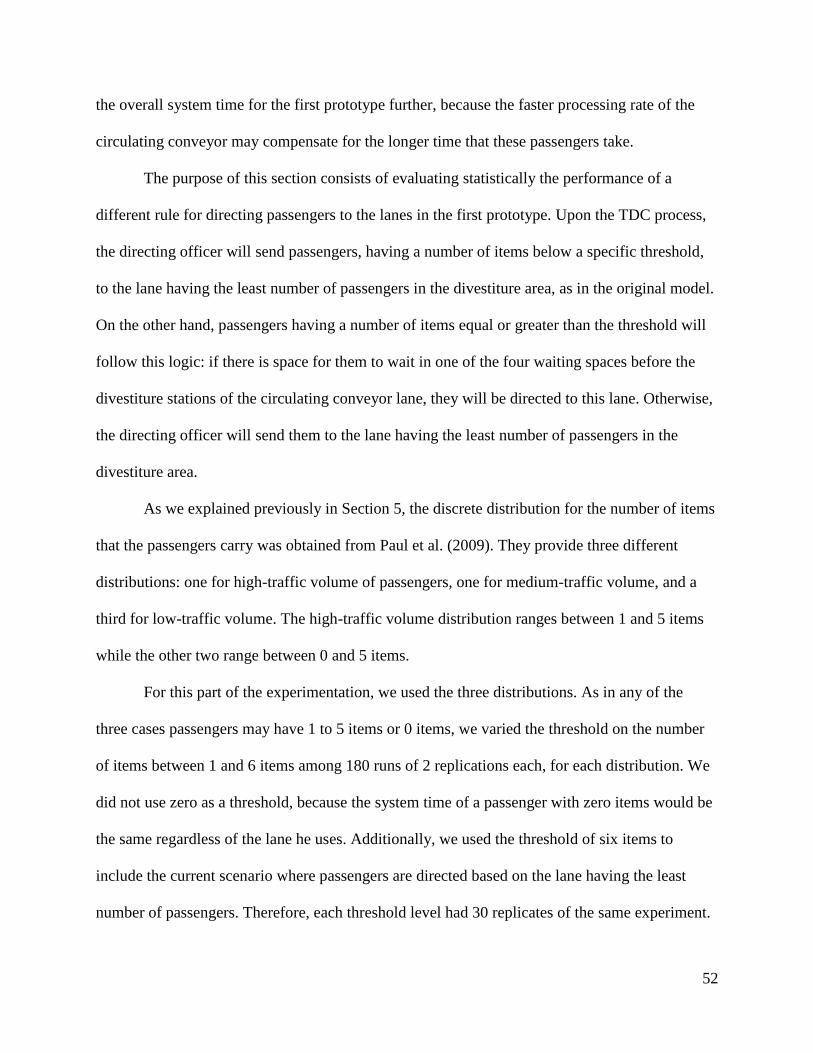
52
the overall system time for the first prototype further, because the faster processing rate of the
circulating conveyor may compensate for the longer time that these passengers take.
The purpose of this section consists of evaluating statistically the performance of a
different rule for directing passengers to the lanes in the first prototype. Upon the TDC process,
the directing officer will send passengers, having a number of items below a specific threshold,
to the lane having the least number of passengers in the divestiture area, as in the original model.
On the other hand, passengers having a number of items equal or greater than the threshold will
follow this logic: if there is space for them to wait in one of the four waiting spaces before the
divestiture stations of the circulating conveyor lane, they will be directed to this lane. Otherwise,
the directing officer will send them to the lane having the least number of passengers in the
divestiture area.
As we explained previously in Section 5, the discrete distribution for the number of items
that the passengers carry was obtained from Paul et al. (2009). They provide three different
distributions: one for high-traffic volume of passengers, one for medium-traffic volume, and a
third for low-traffic volume. The high-traffic volume distribution ranges between 1 and 5 items
while the other two range between 0 and 5 items.
For this part of the experimentation, we used the three distributions. As in any of the
three cases passengers may have 1 to 5 items or 0 items, we varied the threshold on the number
of items between 1 and 6 items among 180 runs of 2 replications each, for each distribution. We
did not use zero as a threshold, because the system time of a passenger with zero items would be
the same regardless of the lane he uses. Additionally, we used the threshold of six items to
include the current scenario where passengers are directed based on the lane having the least
number of passengers. Therefore, each threshold level had 30 replicates of the same experiment.

53
A separate analysis of variance was conducted for each of the three distributions, testing the
effect of the number of items’ threshold on the total system time. Different from the previous
experimentation section, the response for the system time includes the processing at secondary
screening. In addition, for this section, we are more interested in the results from simultaneously
comparing the mean difference on the system time of all the 15 possible pair combinations
among the six possible thresholds. Figure 31 displays the interval plot of the system time for the
six thresholds, using the high-traffic volume distribution. As we can see, the scenarios with
thresholds of four, five and six items seem to have the shortest mean system time. However, the
threshold resulting in the minimum system time seems to be five items.
Figure 31. Interval Plot on System Time vs. Num. of Items Threshold
(High-Traffic Volume Distribution)
Figure 32 displays the results from simultaneously comparing the mean system time of the six
scenarios. Similar to what we observed in Figure 31, the lowest mean corresponds to the five
items’ threshold. However, the mean system times for the scenarios with thresholds of four and
654321
6.0
5.5
5.0
4.5
4.0
Items Threshold
Syst
em
Tim
e
Interval Plot of System Time vs Items Threshold95% CI for the Mean
The pooled standard deviation was used to calculate the intervals.
54
six items are statistically the same. The scenarios with thresholds of one, two and three items
have statistically different mean system times. However, these system times are inferior to the
system time of the current configuration. Therefore, for the high-traffic volume distribution,
setting a threshold on the number of items to direct passengers to the circulating conveyor lane,
does not make a significant difference in the mean system time of passengers.
Figure 32. Multiple Comparison Test on System Time vs. Num. of Items Threshold
(High-Traffic Volume Distribution)
Figure 33 displays the interval plot of the system time for the scenarios of the medium-traffic
volume distribution. Similar to the plot for the high-traffic volume distribution, the scenarios
with thresholds of four, five and six items have the shortest mean system time. Moreover, the
Tukey’s pairwise comparison test in Figure 34 showed that there is no statistical difference
among the system time of these scenarios. In addition, scenarios with thresholds of one, two and
three items result in a statistically longer system time than the scenario of the current
configuration. Therefore, for a medium-traffic volume distribution, setting a threshold on the
number of items to direct passengers to the circulating conveyor lane, does not improve the
performance of the checkpoint in terms of the mean system time.

55
Figure 33. Interval Plot on System Time vs. Num. of Items Threshold
(Medium-Traffic Volume Distribution)
Figure 34. Multiple Comparison Test on System Time vs. Num. of Items Threshold
(Medium-Traffic Volume Distribution)
Lastly, Figure 35 displays the interval plot of the system time for the low-traffic volume
distribution. Different from the previous two cases, the minimum mean system time is among the
scenarios with thresholds of three, four, five and six items.
654321
3.6
3.4
3.2
3.0
2.8
2.6
2.4
2.2
2.0
Items Threshold
Syst
em
Tim
e
Interval Plot of System Time vs Items Threshold95% CI for the Mean
The pooled standard deviation was used to calculate the intervals.
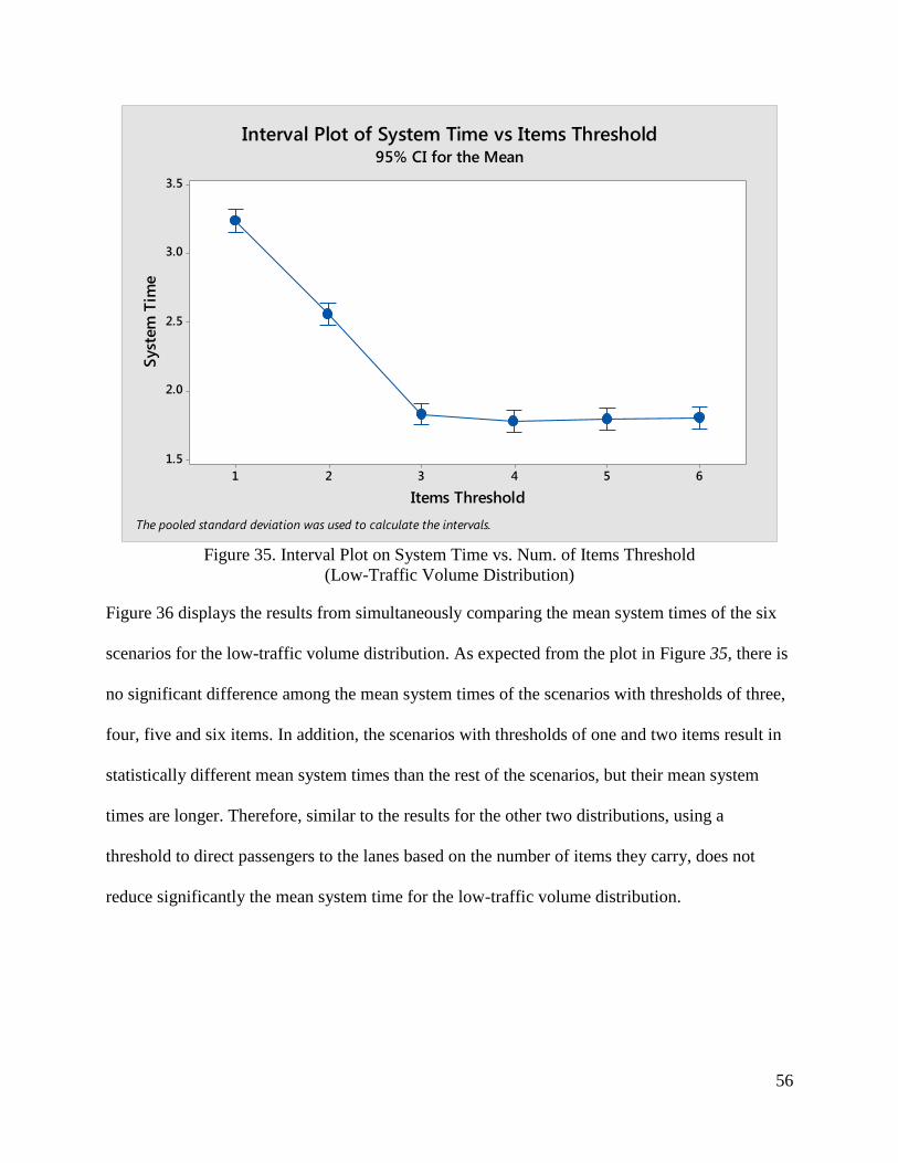
56
Figure 35. Interval Plot on System Time vs. Num. of Items Threshold
(Low-Traffic Volume Distribution)
Figure 36 displays the results from simultaneously comparing the mean system times of the six
scenarios for the low-traffic volume distribution. As expected from the plot in Figure 35, there is
no significant difference among the mean system times of the scenarios with thresholds of three,
four, five and six items. In addition, the scenarios with thresholds of one and two items result in
statistically different mean system times than the rest of the scenarios, but their mean system
times are longer. Therefore, similar to the results for the other two distributions, using a
threshold to direct passengers to the lanes based on the number of items they carry, does not
reduce significantly the mean system time for the low-traffic volume distribution.
654321
3.5
3.0
2.5
2.0
1.5
Items Threshold
Syst
em
Tim
eInterval Plot of System Time vs Items Threshold
95% CI for the Mean
The pooled standard deviation was used to calculate the intervals.
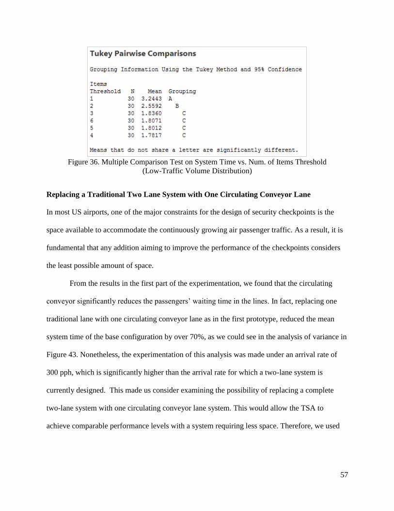
57
Figure 36. Multiple Comparison Test on System Time vs. Num. of Items Threshold
(Low-Traffic Volume Distribution)
Replacing a Traditional Two Lane System with One Circulating Conveyor Lane
In most US airports, one of the major constraints for the design of security checkpoints is the
space available to accommodate the continuously growing air passenger traffic. As a result, it is
fundamental that any addition aiming to improve the performance of the checkpoints considers
the least possible amount of space.
From the results in the first part of the experimentation, we found that the circulating
conveyor significantly reduces the passengers’ waiting time in the lines. In fact, replacing one
traditional lane with one circulating conveyor lane as in the first prototype, reduced the mean
system time of the base configuration by over 70%, as we could see in the analysis of variance in
Figure 43. Nonetheless, the experimentation of this analysis was made under an arrival rate of
300 pph, which is significantly higher than the arrival rate for which a two-lane system is
currently designed. This made us consider examining the possibility of replacing a complete
two-lane system with one circulating conveyor lane system. This would allow the TSA to
achieve comparable performance levels with a system requiring less space. Therefore, we used
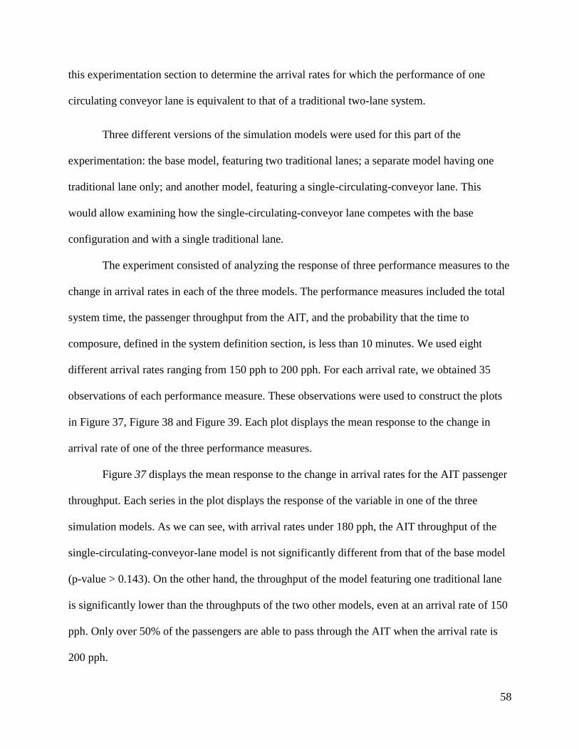
58
this experimentation section to determine the arrival rates for which the performance of one
circulating conveyor lane is equivalent to that of a traditional two-lane system.
Three different versions of the simulation models were used for this part of the
experimentation: the base model, featuring two traditional lanes; a separate model having one
traditional lane only; and another model, featuring a single-circulating-conveyor lane. This
would allow examining how the single-circulating-conveyor lane competes with the base
configuration and with a single traditional lane.
The experiment consisted of analyzing the response of three performance measures to the
change in arrival rates in each of the three models. The performance measures included the total
system time, the passenger throughput from the AIT, and the probability that the time to
composure, defined in the system definition section, is less than 10 minutes. We used eight
different arrival rates ranging from 150 pph to 200 pph. For each arrival rate, we obtained 35
observations of each performance measure. These observations were used to construct the plots
in Figure 37, Figure 38 and Figure 39. Each plot displays the mean response to the change in
arrival rate of one of the three performance measures.
Figure 37 displays the mean response to the change in arrival rates for the AIT passenger
throughput. Each series in the plot displays the response of the variable in one of the three
simulation models. As we can see, with arrival rates under 180 pph, the AIT throughput of the
single-circulating-conveyor-lane model is not significantly different from that of the base model
(p-value > 0.143). On the other hand, the throughput of the model featuring one traditional lane
is significantly lower than the throughputs of the two other models, even at an arrival rate of 150
pph. Only over 50% of the passengers are able to pass through the AIT when the arrival rate is
200 pph.
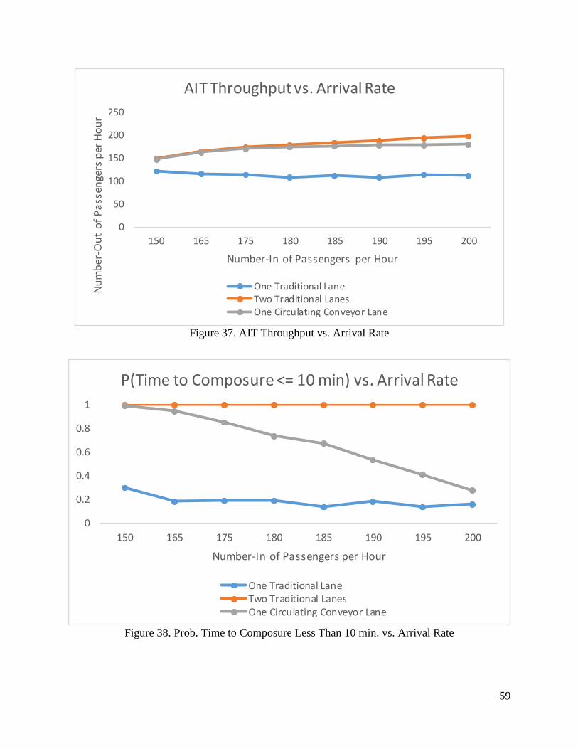
59
Figure 37. AIT Throughput vs. Arrival Rate
Figure 38. Prob. Time to Composure Less Than 10 min. vs. Arrival Rate
0
50
100
150
200
250
150 165 175 180 185 190 195 200
Nu
mb
er-O
ut
of
Pa
ssen
gers
per
Ho
ur
Number-In of Passengers per Hour
AIT Throughput vs. Arrival Rate
One Traditional LaneTwo Traditional LanesOne Circulating Conveyor Lane
0
0.2
0.4
0.6
0.8
1
150 165 175 180 185 190 195 200
Number-In of Passengers per Hour
P(Time to Composure <= 10 min) vs. Arrival Rate
One Traditional LaneTwo Traditional LanesOne Circulating Conveyor Lane
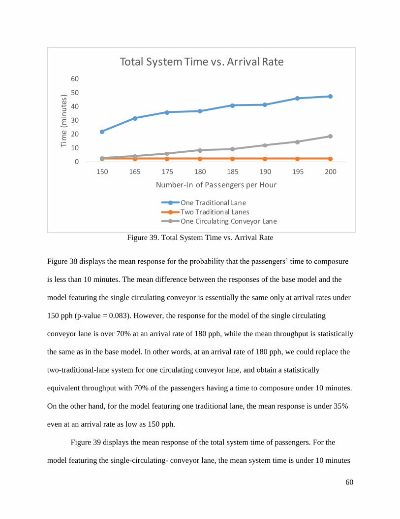
60
Figure 39. Total System Time vs. Arrival Rate
Figure 38 displays the mean response for the probability that the passengers’ time to composure
is less than 10 minutes. The mean difference between the responses of the base model and the
model featuring the single circulating conveyor is essentially the same only at arrival rates under
150 pph (p-value = 0.083). However, the response for the model of the single circulating
conveyor lane is over 70% at an arrival rate of 180 pph, while the mean throughput is statistically
the same as in the base model. In other words, at an arrival rate of 180 pph, we could replace the
two-traditional-lane system for one circulating conveyor lane, and obtain a statistically
equivalent throughput with 70% of the passengers having a time to composure under 10 minutes.
On the other hand, for the model featuring one traditional lane, the mean response is under 35%
even at an arrival rate as low as 150 pph.
Figure 39 displays the mean response of the total system time of passengers. For the
model featuring the single-circulating- conveyor lane, the mean system time is under 10 minutes
0
10
20
30
40
50
60
150 165 175 180 185 190 195 200
Tim
e (m
inu
tes)
Number-In of Passengers per Hour
Total System Time vs. Arrival Rate
One Traditional LaneTwo Traditional LanesOne Circulating Conveyor Lane
61
for arrival rates under 185 pph. Nonetheless, for arrival rates ranging from 185 pph to 200 pph,
the mean system time remains under 20 minutes. On the other hand, for the one-traditional-lane
system, the system time is over 20 minutes when the arrival rate is 150 pph, and it reaches over
45 minutes when the arrival rate is 200 pph.
Therefore, the single-circulating conveyor lane clearly outperforms the single-traditional
–lane system. On the other hand, whether the single-circulating-conveyor lane could replace a
traditional two-lane system depends on the decision maker’s tolerance level with respect to the
checkpoint performance. For instance, if the decision maker is willing to accept an 85%
probability that the time to composure is less than 10 minutes, the single-circulating-conveyor-
lane system can replace the base model, and achieve the same throughput performance with
arrival rates under 175 pph.
CONCLUSION AND FUTURE WORK
In a previous effort (Janer and Rossetti 2016), we found that replacing the exit roller for a
circulating conveyor could increase the processing rate of passengers through the checkpoints by
28%. This study consisted of examining the effect of this circulating conveyor on the secondary
screening process, as this element of the checkpoint was not considered previously. In addition,
for a two-lane system where one lane features the traditional exit roller while the other lane
features the circulating conveyor, we evaluated whether there could be any improvements in the
passengers’ system time from directing the passengers to the lanes based on the number of items
they carry. Moreover, we examined the arrival rates for which a single circulating conveyor lane
could achieve equivalent performance to that of a traditional two-lane system.
Three simulation models were developed for this study. The base model represented the
current configuration, where items coming from the x-ray are delivered to an exit roller in both
62
lanes of a mirror-two-lane system. The second model corresponds to the first prototype. This is
also a two-lane system, but one lane features the traditional exit roller while the other lane
features the circulating conveyor. The third model corresponds to the second prototype. This is a
mirror-two-lane system, where the two lanes feature the circulating conveyor at the composure
area.
In the first part of the experimentation, using an analysis of variance on the x-ray
processing limit, we found that a limit of 15 seconds results in a shorter system time than a limit
of 30 seconds and a limit of 7 seconds. Nonetheless, limits of 30 and 45 seconds result in
essentially the same mean system time. Note the system time for the first portion of the
experimentation did not include the time in secondary screening. To find the limit resulting in the
minimum system time, we fitted a univariate response curve to 176 observations of the system
time under different limits. We found that the critical point of the curve resulting in the minimum
system time was 18 seconds. Sensitivity analysis was performed on this optimum limit using the
coefficient of variation of the secondary screening distribution and the prototypes models.
Although we did not construct a confidence interval on the optimum limit, it seemed that
increasing the coefficient of variation of the secondary screening distribution resulted in a
smaller optimum limit. In other words, reducing the mean of the distribution reduced the risk
associated with failing to identify a threat, because the optimum limit was smaller. A smaller
optimum limit increases the probability that an item requires secondary screening. Future work
of this study should include developing confidence intervals on the optimum limits obtained
from optimizing the univariate response curves. Through an additional analysis of variance, we
found that the mean of the secondary screening distribution does not have a significant effect on
the system time when the limit is at the optimum level. In addition, the results from the
63
sensitivity analysis on the optimum limit, using the first and seconds prototype models, showed
that the prototypes do not have any effect on the optimum x-ray processing time limit.
Nonetheless, the models significantly decreased the minimum system time under the optimum x-
ray processing time limit of each model. The first prototype resulted in a mean system time 70%
shorter than that of the base model, while the second prototype resulted a mean system time 16
% shorter than that of the first prototype.
For the second portion of the experimentation, we evaluated the effect of six different
thresholds on the number of items used to direct passengers to the circulating conveyor lane in
the first prototype. We used a Tukey’s multiple comparison test to compare simultaneously the
mean system time of passengers for the six different thresholds. Different from the first portion
of the experimentation, the system time response for this portion included the secondary
screening process. We repeated this analysis for three different distributions on the number of
items per passengers, obtained from Paul et al. (2009). For the three distributions, we obtained
that the minimum system time was among the scenarios with thresholds on four, five and six
items. The latest corresponds to the current scenario, where passengers are directed to the lane
having the least number of passengers in the divestiture area. The mean difference among the
three best scenarios was not significant for any of the three distributions. Therefore, directing
passengers to the circulating conveyor lane, using a threshold on the number of items per
passenger, does not significantly reduce the mean system time.
For the last portion of the experimentation, we found that for arrival rates under 180 pph,
the mean probability that the passengers’ time to composure is under 10 minutes was 30% lower
for a single circulating conveyor lane than for the traditional two-lane system. Nonetheless, the
throughput was statistically the same for both models. In addition, the mean system time for the
64
model featuring the single circulating conveyor lane was under 10 minutes. Thus, if the TSA is
willing to tolerate a decrease in 30% in the probability that passengers have a time to composure
within 10 minutes, they could replace the traditional two-lane system for a single circulating
conveyor lane for checkpoints where the arrival per AIT is less or equal to 180 pph.
Future work on this study should consider developing response surfaces to optimize the
key metrics of a checkpoint performance. Independent factors for this response surface analysis
should include the three simulation models, and the distributions of the secondary screening
process, the x-ray inspection time and the TDC process, as these are the checkpoint elements
with the highest utilization in the current configuration and the two prototypes.
65
REFERENCES
Blalock, G., V. Kadiyali, and D. H. Simon. The Impact of Post-9 / 11 Airport Security Measures
on the Demand for Air Travel. Journal of Law and Economics, Vol. 50, No. 4, 2007, pp.
31–755.
De Barros, A. G., and D. D. Tomber. Quantitative Analysis of Passenger and Baggage Security
Screening at Airports. Journal of Advanced Transportation, Vol. 41, No. 2, 2007, pp
171–193.
Cahya, S., E. Del Castillo, and J. J. Peterson. Computation of Confidence Regions for Optimal
Factor Levels in Constrained Response Surface Problems. Journal of Computational and
Graphical Statistics, Vol. 13, No. 2, 2004, pp. 499-518.
De Lange, R., I. Samoilovich, and B. V. Der Rhee. Virtual Queuing at Airport Security Lanes.
European Journal of Operational Research, Vol. 225, No. 1, 2013, pp 153–165.
DFW Planning Department. Dallas/Fort Worth Security Checkpoints - Tiger Team 2005 -
Improving Throughput, July 2006.
https://www.dfwairport.com/dfwucm1prd/groups/public/documents/webasset/p1_008154
.pdf. Accessed January 17, 2017
Doran, D., S. Gokhale, and N. Lownes. Analytic Model of Screening Times at Airport Security
Checkpoints. In Transportation Research Record: Journal of the Transportation
Research Board. No. 2400, Transportation Research Board of the National Academies,
Washington, D.C., 2013, pp 1–8.
Dorton, S. L., and D. Liu. Effects of Baggage Volume and Alarm Rate on Airport Security
Screening Checkpoint Efficiency Using Queuing Networks and Discrete Event
Simulation. Human Factors and Ergonomics in Manufacturing, Vol. 26, No. 1, 2016, pp
95–109.
Fayez, M.S., et al. Managing Airport Operations Using Simulation. Journal of Simulation Vol. 2,
No.1, 2008, pp 41–52.
Guru, A., and P. Savory. A Template-Based Conceptual Modeling Infrastructure for Simulation
of Physical Security Systems. Proceedings of the 2004 Winter Simulation Conference,
2004, pp 866-873.
Hobbs, B., M. D. Rossetti, P. Faas. (2006) An Object-Oriented Framework For Simulating
Automatic Data Collection Systems, The Proceedings of the 2006 Winter Simulation
Conference, L. F. Perrone, F. P. Wieland, J. Liu, B. G. Lawson, D. M. Nicol, and R. M.
Fujimoto, eds., Piscataway, New Jersey: Institute of Electrical and Electronic Engineers
Leone, K., and R. Liu. Improving Airport Security Screening Checkpoint Operations in the US
via Paced System Design. Journal of Air Transport Management, Vol. 17, No. 2, 2011,
pp 62–67.

66
Nie, X., et al. Simulation-Based Selectee Lane Queueing Design for Passenger Checkpoint
Screening. European Journal of Operational Research, Vol. 219, No. 1, 2012, pp 146–
155.
Paul, J. A., et al. Airport Security System Design: Passenger Flow Analysis and Simulation
Modeling. Protecting Airline Passengers in the Age of Terrorism, ABC- Clio, Santa
Barbara, CA, 2009. Edited by Paul Seidenstat and Francis X. Splane.
Pendergraft, D. R., C. V. Robertson, and S. Shrader. Simulation of an Airport Passenger Security
System. Proceedings of the 2004 Winter Simulation Conference, 2004, pp 874–878.
Price, H. FAA Forecast Sees Continued, Steady Growth in Air Travel. Federal Aviation Administration,
March 2015.
Solomon, R. TSA chief: Delta innovation lanes make ‘dramatic improvements’, June 2016.
http://news.delta.com/tsa-chief-delta-innovation-lanes-make-dramatic-improvements.
TSA Pre-Check Expansion Act. Report of the Committee on Commerce, Science, and
Transportation on H. R. 2843. 2016. https://www.congress.gov/bill/114th-
congress/house-bill/2843/
Wan, F., et al. An Exact Confidence Set for a Maximum Point of a Univariate Polynomial
Function in a given Interval. Technometrics, Vol. 57, No. 4, pp 559-565.
Wetter, O. E., M. Lipphardt, and F. Hofer. External and Internal Influences on the Security
Control Process at Airports. Proceedings – IEEE International Carnahan Conference on
Security Technology, 2010, pp 301–309.
Wilson, D., E. K. Roe, and S. A. So. Security Checkpoint Optimizer (SCO): An Application for
Simulating the Operations of Airport Security Checkpoints. Proceedings of the 2006
Winter Simulation Conference, 2006, pp 529–535.
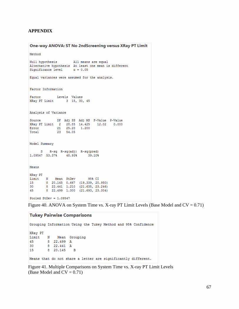
67
APPENDIX
Figure 40. ANOVA on System Time vs. X-ray PT Limit Levels (Base Model and CV = 0.71)
Figure 41. Multiple Comparisons on System Time vs. X-ray PT Limit Levels
(Base Model and CV = 0.71)
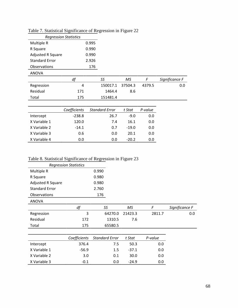
68
Table 7. Statistical Significance of Regression in Figure 22
Regression Statistics
Multiple R 0.995
R Square 0.990
Adjusted R Square 0.990
Standard Error 2.926
Observations 176
ANOVA
df SS MS F Significance F
Regression 4 150017.1 37504.3 4379.5 0.0
Residual 171 1464.4 8.6
Total 175 151481.4
Coefficients Standard Error t Stat P-value
Intercept -238.8 26.7 -9.0 0.0
X Variable 1 120.0 7.4 16.1 0.0
X Variable 2 -14.1 0.7 -19.0 0.0
X Variable 3 0.6 0.0 20.1 0.0
X Variable 4 0.0 0.0 -20.2 0.0
Table 8. Statistical Significance of Regression in Figure 23
Regression Statistics
Multiple R 0.990
R Square 0.980
Adjusted R Square 0.980
Standard Error 2.760
Observations 176
ANOVA
df SS MS F Significance F
Regression 3 64270.0 21423.3 2811.7 0.0
Residual 172 1310.5 7.6
Total 175 65580.5
Coefficients Standard Error t Stat P-value
Intercept 376.4 7.5 50.3 0.0
X Variable 1 -56.9 1.5 -37.1 0.0
X Variable 2 3.0 0.1 30.0 0.0
X Variable 3 -0.1 0.0 -24.9 0.0
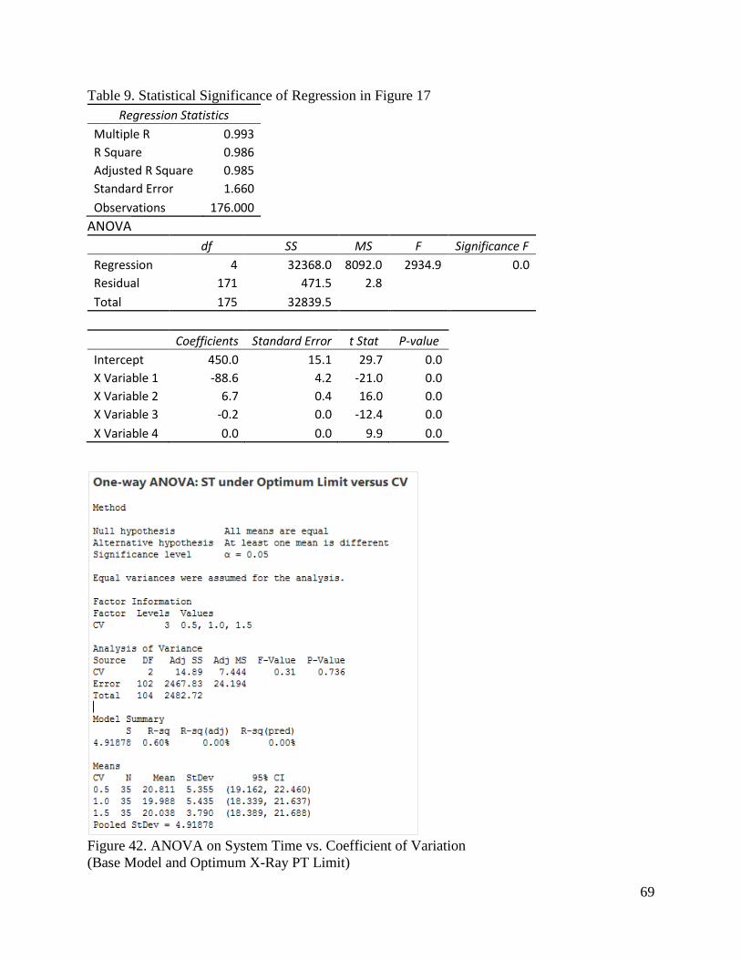
69
Table 9. Statistical Significance of Regression in Figure 17
Regression Statistics
Multiple R 0.993
R Square 0.986
Adjusted R Square 0.985
Standard Error 1.660
Observations 176.000
ANOVA
df SS MS F Significance F
Regression 4 32368.0 8092.0 2934.9 0.0
Residual 171 471.5 2.8
Total 175 32839.5
Coefficients Standard Error t Stat P-value
Intercept 450.0 15.1 29.7 0.0
X Variable 1 -88.6 4.2 -21.0 0.0
X Variable 2 6.7 0.4 16.0 0.0
X Variable 3 -0.2 0.0 -12.4 0.0
X Variable 4 0.0 0.0 9.9 0.0
Figure 42. ANOVA on System Time vs. Coefficient of Variation
(Base Model and Optimum X-Ray PT Limit)
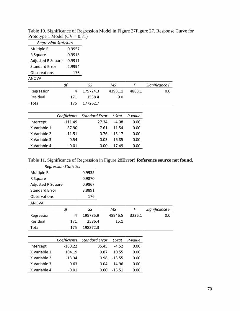
70
Table 10. Significance of Regression Model in Figure 27Figure 27. Response Curve for
Prototype 1 Model (CV = 0.71)
Regression Statistics
Multiple R 0.9957
R Square 0.9913
Adjusted R Square 0.9911
Standard Error 2.9994
Observations 176
ANOVA
df SS MS F Significance F
Regression 4 175724.3 43931.1 4883.1 0.0
Residual 171 1538.4 9.0
Total 175 177262.7
Coefficients Standard Error t Stat P-value
Intercept -111.49 27.34 -4.08 0.00
X Variable 1 87.90 7.61 11.54 0.00
X Variable 2 -11.51 0.76 -15.17 0.00
X Variable 3 0.54 0.03 16.85 0.00
X Variable 4 -0.01 0.00 -17.49 0.00
Table 11. Significance of Regression in Figure 28Error! Reference source not found.
Regression Statistics
Multiple R 0.9935
R Square 0.9870
Adjusted R Square 0.9867
Standard Error 3.8891
Observations 176
ANOVA
df SS MS F Significance F
Regression 4 195785.9 48946.5 3236.1 0.0
Residual 171 2586.4 15.1
Total 175 198372.3
Coefficients Standard Error t Stat P-value
Intercept -160.22 35.45 -4.52 0.00
X Variable 1 104.19 9.87 10.55 0.00
X Variable 2 -13.34 0.98 -13.55 0.00
X Variable 3 0.63 0.04 14.96 0.00
X Variable 4 -0.01 0.00 -15.51 0.00

71
Figure 43. ANOVA on System Time vs. Models (CV = 0.71 and Optimum X-Ray PT Limit)
Figure 44. Multiple Comparison Test on System Time vs. Models
(CV = 0.71 and Optimum X-Ray PT Limit)