analytical integrate-and-fire neuron models with ...cns.iaf.cnrs-gif.fr/files/gif2011.pdf · letter...
TRANSCRIPT

LETTER Communicated by Benjamin Schrauwen
Analytical Integrate-and-Fire Neuron Models withConductance-Based Dynamics and RealisticPostsynaptic Potential Time Course for Event-DrivenSimulation Strategies
Michelle [email protected] [email protected] [email protected] de Neuroscience Integratives et Computationnelles, CNRS,91198 Gif-sur-Yvette, France
In a previous paper (Rudolph & Destexhe, 2006), we proposed variousmodels, the gIF neuron models, of analytical integrate-and-fire (IF) neu-rons with conductance-based (COBA) dynamics for use in event-drivensimulations. These models are based on an analytical approximationof the differential equation describing the IF neuron with exponentialsynaptic conductances and were successfully tested with respect to theirresponse to random and oscillating inputs. Because they are analyticaland mathematically simple, the gIF models are best suited for fast event-driven simulation strategies. However, the drawback of such models isthey rely on a nonrealistic postsynaptic potential (PSP) time course, con-sisting of a discontinuous jump followed by a decay governed by themembrane time constant. Here, we address this limitation by conceivingan analytical approximation of the COBA IF neuron model with the fullPSP time course. The subthreshold and suprathreshold response of thisgIF4 model reproduces remarkably well the postsynaptic responses of thenumerically solved passive membrane equation subject to conductancenoise, while gaining at least two orders of magnitude in computationalperformance. Although the analytical structure of the gIF4 model is morecomplex than that of its predecessors due to the necessity of calculatingfuture spike times, a simple and fast algorithmic implementation for usein large-scale neural network simulations is proposed.
1 Introduction
Event-driven (or asynchronous) simulation strategies have establishedthemselves as an efficient and potent alternative to traditional clock-driven
Neural Computation 24, 1426–1461 (2012) c© 2012 Massachusetts Institute of Technology

The gIF4 Method 1427
(or synchronous) strategies (Watts, 1994; Mattia & Del Giudice, 2000; Reuti-mann, Giugliano, & Fusi, 2003; Brette, 2006, 2007; Tonnelier, Belmabrouk,& Martinez, 2007; Carrillo, Ros, Tolu, Nieus, & D’Angelo, 2008; D’Haene,Schrauwen, Van Campenhout, & Stroobandt, 2009), particularly in com-putational investigations of biologically more realistic large-scale neuralnetworks (for a comprehensive overview, see Brette et al., 2007). One defin-ing advantage of such strategies is the exact treatment of spike times,which renders simulations of complex neural systems more precise thanachievable in traditional clock-driven numerical integration approaches(Tsodyks, Mit’kov, & Sompolinsky, 1993; Hansel, Mato, Meurier, & Neltner,1998; Markram, Wang, & Tsodyks, 1998; Senn, Markram, & Tsodyks, 2000;Rudolph & Destexhe, 2007). However, the exploitation of this advantagesets stringent requirements to the neuronal models used. Specifically, tomake full use of the activity-dependent gains in speed of neural simula-tions implementing the event-driven strategy, the neuronal models must beanalytically solvable, or at least provide analytically simple approximationsfor their state variables.
Despite such constraints, the event-driven approach was successfully ap-plied in a variety of contexts. These range from networks of spiking neuronswith complex dynamics and focused on hardware implementations (Watts,1994; Giugliano, 2000; Mattia & Del Giudice, 2000) or specific software im-plementations (Carrillo et al., 2008), up to networks of several hundredthousand neurons modeling the processing of information in the visualcortex (Delorme, Gautrais, van Rullen, & Thorpe, 1999; Delorme & Thorpe,2003). Other studies focused on easing the constraints imposed on the com-plexity of the used neuronal models by demonstrating that the event-drivenframework can be applied to integrate-and-fire (IF) neurons with exponen-tial synaptic conductances (Brette, 2006, 2007; Rudolph & Destexhe, 2007),that is, models whose solutions are no longer given in terms of closed-formanalytically exact functions, that is, functions not containing infinite sums orintegrals in their analytical definition. Simulations with such models wereshown to yield more exact results and were computationally more efficientwhen compared with classical integration schemes such as Euler or Runge-Kutta commonly used in clock-driven simulation strategies (Brette, 2006).Finally, the event-driven approach was successfully extended to models ofneuronal dynamics described by stochastic processes, such as intrinsicallynoisy neurons or neurons with synaptic noise stemming from their em-bedding into larger networks (Reutimann et al., 2003), thus providing anefficient simulation strategy for studying networks of interacting neuronswith an arbitrary number of external afferents modeled in terms of effectivestochastic processes (Ricciardi & Sacerdote, 1979; Lansky & Rospars, 1995;Destexhe, Rudolph, Fellous, & Sejnowski, 2001).
Originally, neuronal models for implementation in event-driven sim-ulations required simple, current-based (CUBA) dynamics (Mattia & DelGiudice, 2000; Reutimann et al., 2003; Hines & Carnevale, 2004) for the full

1428 M. Rudolph-Lilith, M. Dubois, and A. Destexhe
exploitation of the computational efficiency of this strategy. More biophys-ically realistic neuronal models with conductance-based (COBA) synapticinteractions or membrane dynamics in general do not allow for an analyt-ically closed-form solution due to the multiplicative coupling of conduc-tances to the state variable. Specifically, even for simple synaptic conduc-tances models, such as exponential decay, despite the fact that the first-orderdifferential membrane equation will yield an analytical solution in termsof special functions, such as gamma functions, the latter can be evaluatedonly numerically or by analytic approximations. This might render suchmodels less suitable for use in event-driven simulations due to the reducednumerical precision (when striving for low computational load) or addi-tional computational load (when striving for higher numerical precision)that accompanies such numerical or analytical approximations.
We have proposed in another paper (Rudolph & Destexhe, 2006) a num-ber of analytical approximations of the leaky classical IF neuron (Lapicque,1907; Knight, 1972) with conductance-based synaptic dynamics, the gIFmodels, in order to overcome this limitation. As we showed, a straightfor-ward analytical approximation of the full solution of the passive membraneequation with exponential inhibitory and excitatory synaptic conductancescan lead to analytically simple closed-form solutions for the state variablein between two succeeding synaptic inputs. In a comparative evaluation,we further showed that the proposed gIF models performed similar tosimple but biophysically unrealistic CUBA leaky IF models, thus gainingseveral orders of magnitude in performance when compared to numericalsolutions of COBA IF neuronal models, while displaying a biophysicallyresponse dynamics to a variety of synaptic input paradigms that was com-parable to COBA models, or even close to that observed in model withHodgkin-Huxley spike-generating mechanisms.
The compromise between performance and precision of the gIF neuronmodels was achieved by using an instantaneous jump of the state variableon arrival of a synaptic input. This freed the algorithm from estimatingspike times, as here spikes can occur only at times of excitatory synapticarrivals and led to an efficient, straightforward implementation in simula-tions using the event-driven framework. However, this compromise alsolimits the possible response dynamics of the original gIF models: neuronalmembranes do display postsynaptic potentials (PSPs), that is, postsynaptictime courses in response to synaptic stimulation with a finite rise time,which may result in spikes occurring up to several milliseconds afterarrival of an excitatory synaptic input.
In this letter, we propose an extension of the original gIF neuronal mod-els, the gIF4 neuronal model, which overcomes this restriction and approxi-mates to high precision the PSP time course and resulting spiking responses.The idea behind the gIF4 model was proposed earlier (Rudolph & Destexhe,2006, appendix C.1) and can be motivated as an analytical implementationof a biophysically plausible neuronal model with state dynamics driven
The gIF4 Method 1429
by synaptic conductances. Although the gIF4 is analytically slightly morecomplex than its predecessors, we show that the model can easily be im-plemented in efficient event-driven simulations achieving a performancecomparable to analytically solved CUBA leaky IF neuronal models, whiledisplaying a subthreshold and suprathreshold response that reproduceswith a high degree of precision the behavior of the numerically solvedpassive membrane equation with COBA synaptic dynamics.
In the following section, we briefly review the idea behind the originalgIF neuronal models before introducing the gIF4 model and the outline ofan algorithm for embedding this model in event-driven simulations. Sec-tion 3 evaluates the response of the gIF4 model to various paradigms ofsynaptic activity in comparison with the numerical solution of the origi-nal membrane equation with conductance-based synaptic inputs. A pre-liminary version of this work was published in a conference proceedings(Rudolph-Lilith, Dubois, & Destexhe, 2009).
2 Analytical Integrate-and-Fire Neuron Models withPresynaptic-Activity Dependent State Dynamics
After a brief review of the original integrate-and-fire (IF) neuron model withpresynaptic-activity-dependent state dynamics (the gIF1 to gIF3 models) insection 2.1, we introduce a new class of model, the gIF4 model, in section2.2.
2.1 Overview of the Original gIF1 to gIF3 Neuron Models. One of thefirst and analytically solvable neuronal models is the leaky integrate-and-fire (LIF) neuron (Lapicque, 1907; Knight, 1972). It describes the dynamicsof the state variable, the membrane potential V(t), in terms of a lineardifferential equation of first order in time:
CdV(t)
dt+ C
τ Lm
(V(t) − VL) = Is(t). (2.1)
Here, C denotes the membrane capacity, τ Lm the (time-independent) time
constant of the leaky membrane, τ Lm = C
GL, with GL being the constant leak
conductance and VL the leak reversal potential. The state variable V(t)takes values between a resting and threshold value, Vrest = VL and Vthres,respectively, and undergoes transient changes driven by the synaptic inputcurrent Is(t). If V(t) reaches the threshold value Vthres at some time t, thecell generates a spike, and V(t) is instantaneously or after a fixed refractoryperiod reset to Vrest.
For sufficiently simple synaptic currents Is(t), equation 2.1 can be solvedanalytically. This, together with the simple update rule of the state variableupon threshold crossings, allows an efficient implementation of this model
1430 M. Rudolph-Lilith, M. Dubois, and A. Destexhe
in event-based numerical simulations. However, synaptic transmission inbiological neurons is conductance based, which renders the synaptic currentIs(t) the result of rapid transient changes of conductances in the postsynap-tic membrane and, thus, dependent on the actual state of the membrane.Denoting with Gs(t) the synaptic conductance and Vs the correspondingsynaptic reversal potential, Is(t) takes the form
Is(t) = −(V(t) − Vs)Gs(t). (2.2)
Due to the coupling of the membrane state V(t) to the synaptic in-put Gs(t) in equation 2.2, these COBA neuronal models are more difficultto solve analytically, and numerical methods remain the standard tech-nique for dealing with such biophysically more realistic dynamics. Variousstudies in the past focused on incorporating this time-dependent or state-dependent aspect of neuronal membranes. As the membrane conductanceis inversely linked to the membrane time constant, a straightforward gener-alization of the classic leaky IF neuronal model can be obtained by using aspike-time dependent membrane time constant (Wehmeier, Dong, Koch, &van Essen, 1989; LeMasson, Marder, & Abbott, 1993; Stevens & Zador, 1998a;Giugliano, Bove, & Grattarola, 1999; Jolivet, Lewis, & Gerstner, 2004). Themost prominent model in this direction is the spike response model (Ger-stner & van Hemmen, 1992, 1993; Gerstner, Ritz, & van Hemmen, 1993;Gerstner & Kistler, 2002). Here, the membrane conductance is increasedright after a postsynaptic spike as a result of the contribution of ion chan-nels linked to spike generation, thus resulting in a transient reduction of themembrane time constant. This reduction shapes the amplitude and formof subsequent postsynaptic potentials (for experimental studies showinga dependence of the PSP shape on intrinsic membrane conductances, seeNicoll, Larkman, & Blakemore, 1993; Stuart & Spruston, 1998) and makesthe response of the membrane to subsequent synaptic inputs dependent onthe history of the cellular activity.
Although the latter can be viewed as a direct consequence of the presy-naptic activity, the mathematical model of the spike response model doesnot include synaptic conductances explicitly and considers the membranetime constant solely as a function of the time since the last postsynapticspike and, thus, the postsynaptic activity. In contrast, other studies focusedon describing the postsynaptic membrane dynamics on an analytical levelas a function of synaptic inputs, thus explicitly in terms of the presynapticactivity. Although both synaptic (hence, directly presynaptic activity de-termined) and spike-generating (hence, directly postsynaptic activity de-termined) conductance contributions can be considered within a similarmathematical framework, our study focuses solely on synaptic conduc-tances and their impact on neural dynamics.
In a recent contribution, the full passive membrane equation with bothinhibitory and excitatory synaptic conductances described by exponential

The gIF4 Method 1431
transients was solved in terms of incomplete gamma integrals, for whichnumerical libraries for fast numerical computation are available. More-over, these libraries provide solutions that are superior in precision whencompared with numerical solutions of the differential equation using, forinstance, Euler or Runge-Kutta integration methods (Brette, 2006). We useda similar approach in our previous paper (Rudolph & Destexhe, 2006), inthat the passive membrane equation with exponential synaptic conduc-tances was solved analytically in terms of gamma functions. However, weused this solution as the starting point for an analytical approximation,which provided a mathematically simple and reasonably exact expressionfor the membrane potential time course on arrival of synaptic inputs.
Specifically, inserting equation 2.2 and denoting with τ sm(t) = C
Gs(t)the
synaptic contribution to the membrane time constant, the state equation 2.1of the leaky IF neuron takes the form
τm(t)dV(t)
dt+ (V(t) − Vrest (t)) = 0, (2.3)
where τm(t) denotes the total time-dependent membrane time constant dueto leak and synaptic conductances,
τm(t) = τ Lmτ s
m(t)τ L
m + τ sm(t)
, (2.4)
and Vrest (t) the time-dependent resting potential,
Vrest (t) = VLτsm(t) + Vsτ
Lm
τ Lm + τ s
m(t). (2.5)
For reasonably simple synaptic conductance models, such as exponentialsynapses, for which the change of the conductance and, hence, time constantupon arrival of a synaptic input at time t0 is described by an instantaneouschange with constant amplitude �τ s
m,
1τ s
m(t0)−→ 1
τ sm(t0)
+ 1�τ s
m, (2.6)
followed by an exponential decay with time constant τs,
1τ s
m(t)= 1
τ sm(t0)
e− t−t0
τs for t ≥ t0, (2.7)
equation 2.3 yields a closed-form solution in terms of incomplete gammafunctions (see appendix B.1 in Rudolph & Destexhe, 2006). The latter was

1432 M. Rudolph-Lilith, M. Dubois, and A. Destexhe
then approximated (for details, see appendix B.2 in Rudolph & Destexhe,2006), yielding a simple analytical expression for the transient changes of thestate variable in between two synaptic inputs as a function of the synapticconductance parameters and the actual state of the membrane.
The analytical form of the obtained approximation of the PSP alloweda simple and efficient implementation in event-driven numerical models.Upon arrival of a synaptic input at time t0, the membrane potential andmembrane time constant are updated according to
V(t0) −→V(t0) + �V(τm(t0),V(t0))
1τm(t0)
= 1τ L
m+ 1
τ sm(t0)
−→ 1τ L
m+ 1
τ sm(t0)
+ 1�τ s
m, (2.8)
respectively. For t > t0 until the next synaptic input at time t1, the membranetime constant “decays” according to
1τm(t)
= 1τ L
m+ 1
τ sm(t0)
e− t−t0
τs for t0 ≤ t < t1 , (2.9)
whereas the state variable follows the time course given by
V(t)=Vrest (t0)+ (V(t0) −Vrest (t0)) exp[− t − t0
τ Lm
− τs
τ sm(t0)
(1 − e
− t−t0τs
)].
(2.10)
In equation 2.8, �V(τm(t0),V(t0)) denotes the (instantaneous) change inthe state variable upon arrival of a synaptic input. In its most gen-eral form (as used in the gIF3 model), this change will depend on boththe actual membrane time constant τm(t0), thus describing the scaling ofthe PSP amplitude as a function of the total membrane conductance, andthe actual state of the membrane V(t0), thus describing the effects of thesynaptic reversal potentials on the amplitude of the PSP.
In a series of numerical simulations, we exposed this newly derived gIFmodel to a variety of synaptic activities and evaluated their spiking re-sponses in comparison with those obtained from numerical solutions of thepassive membrane equation, the leaky IF model and a biophysically morerealistic neuron model incorporating the Hodgkin-Huxley spike-generatingmechanism. It was shown (see Rudolph & Destexhe, 2006) that at leastthe gIF3 model yields responses that reproduce with acceptable accuracyin physiologically relevant parameter regimes the spontaneous dischargestatistics, the temporal precision in resolving synaptic inputs, and gainmodulating behavior under in vivo–like synaptic bombardment seen inmore realistic neuronal models. At the same time, the gIF models remained

The gIF4 Method 1433
several orders of magnitude more efficient to simulate. It was argued thatthis marked gain in a more realistic biophysical dynamics, faithfully cap-turing crucial aspects of high-conductance states in vivo, combined withonly a minor decrease in computational performance when compared toclassical CUBA IF models, justified the use of the gIF neuron models asa useful tool for efficient and precise simulations of large-scale neuronalnetworks with realistic, conductance-based synaptic interactions.
The gIF neuron model was conceived as an approximation of the classicalleaky IF neuron model (the passive membrane equation) with COBA synap-tic inputs. Neither active membrane conductances, such as those consideredin the spike response model (Gerstner & van Hemmen, 1992, 1993; Gerstneret al., 1993; Gerstner & Kistler, 2002), nor simplifications of spike genera-tion mechanism (e.g., based on Hodgkin-Huxley kinetic models; Hodgkin &Huxley, 1952), such as those considered in the various instances of nonlinearIF neuron models (Abbott & van Vreeswijk, 1993; Fourcaud-Trocme, Hansel,van Vreeswijk, & Brunel, 2003; for a general review, see Gerstner & Kistler,2002), were incorporated into the gIF models. The proposed gIF modelsare also different from mathematically more abstract models (Izhikevich,2001, 2003) and will not capture intrinsic phenomena like bursting or spikerate adaptation. Finally, the instantaneous update of the membrane statevariable on arrival of a synaptic input abstracts from a more realistic shapeof the membrane potential following synaptic stimulation (for a model thatconsiders this aspect, see Kuhn, Aertsen, & Rotter, 2004). Therefore, variousaspects of neuronal dynamics, which depend on both the exact form of PSPsor the presence of intrinsic state-dependent membrane currents contribut-ing to spike generation or response adaptation, were not captured by thegIF models proposed previously.
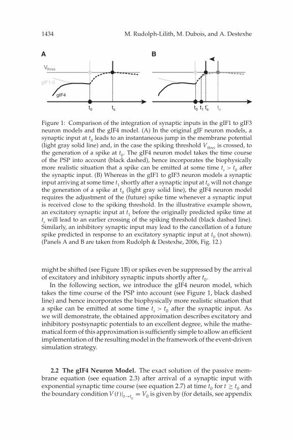
Although the original gIF neuron models, in particular the gIF3 model,reproduced with great accuracy the response statistics to a variety of synap-tic input models in physiologically relevant parameter regimes, great de-viations are expected if the exact times of spikes or more precise temporalaspects of the neuronal response are considered. The main reason for thisis the way these models incorporate the response to a synaptic input. Asshown in Figure 1, in the original gIF models, a synaptic input at t0 leadsto an instantaneous jump in the membrane potential (see Figure 1A, lightgray solid line) and, in the case the spiking threshold Vthres is crossed, to thegeneration of a spike at the same time t0. However, biophysically, the mem-brane generates a PSP transient in response to a synaptic input, which willreach its peak sometime after the synaptic input occurred (see Figure 1A,black dashed line). Thus, in this case, even if the synaptic input drives themembrane above the threshold for spike generation, a spike in response tothis input might be delayed up to several milliseconds. This fact may havecrucial impact in situations that involve, or depend on, the precise timingof spikes. Moreover, in high-conductance regimes with many thousandsof synaptic inputs impinging on the membrane each second, spike times
1434 M. Rudolph-Lilith, M. Dubois, and A. Destexhe
gIF1-3
gIF4
Vthres
tstst1t0tst0
BA
Figure 1: Comparison of the integration of synaptic inputs in the gIF1 to gIF3neuron models and the gIF4 model. (A) In the original gIF neuron models, asynaptic input at t0 leads to an instantaneous jump in the membrane potential(light gray solid line) and, in the case the spiking threshold Vthres is crossed, tothe generation of a spike at t0. The gIF4 neuron model takes the time courseof the PSP into account (black dashed), hence incorporates the biophysicallymore realistic situation that a spike can be emitted at some time ts > t0 afterthe synaptic input. (B) Whereas in the gIF1 to gIF3 neuron models a synapticinput arriving at some time t1 shortly after a synaptic input at t0 will not changethe generation of a spike at t0 (light gray solid line), the gIF4 neuron modelrequires the adjustment of the (future) spike time whenever a synaptic inputis received close to the spiking threshold. In the illustrative example shown,an excitatory synaptic input at t1 before the originally predicted spike time atts will lead to an earlier crossing of the spiking threshold (black dashed line).Similarly, an inhibitory synaptic input may lead to the cancellation of a futurespike predicted in response to an excitatory synaptic input at t0 (not shown).(Panels A and B are taken from Rudolph & Destexhe, 2006, Fig. 12.)
might be shifted (see Figure 1B) or spikes even be suppressed by the arrivalof excitatory and inhibitory synaptic inputs shortly after t0.
In the following section, we introduce the gIF4 neuron model, whichtakes the time course of the PSP into account (see Figure 1, black dashedline) and hence incorporates the biophysically more realistic situation thata spike can be emitted at some time ts > t0 after the synaptic input. Aswe will demonstrate, the obtained approximation describes excitatory andinhibitory postsynaptic potentials to an excellent degree, while the mathe-matical form of this approximation is sufficiently simple to allow an efficientimplementation of the resulting model in the framework of the event-drivensimulation strategy.
2.2 The gIF4 Neuron Model. The exact solution of the passive mem-brane equation (see equation 2.3) after arrival of a synaptic input withexponential synaptic time course (see equation 2.7) at time t0 for t ≥ t0 andthe boundary condition V(t)|t→t0
= V0 is given by (for details, see appendix
The gIF4 Method 1435
B.2 in Rudolph & Destexhe, 2006)
V(t) = exp[− t − t0
τ Lm
+ τs
τ sm(t0)
e− t−t0
τs
]
×{V0 e
− τsτ sm (t0 ) − Vs
(e
− τsτ sm (t0 ) − exp
[t − t0
τ Lm
− τs
τ sm(t0)
e− t−t0
τs
])
−�
[− τs
τ Lm
,τs
τ sm(t0)
e− t−t0
τs ,τs
τ sm(t0)
] (τs
τ sm(t0)
) τsτLm τs
τ Lm
(Vs − VL)
},
(2.11)
where �[z, a, b] = ∫ ba dt tz−1e−t denotes the generalized incomplete gamma
function. Instead of estimating the PSP peak height (or maximum) from thissolution for use as an instantaneous update (or “jump”) of the membranepotential on arrival of a synaptic input, for the gIF4 model we will approx-imate equation 2.11 and the transient changes of the membrane potentialresulting from the arrival of a synaptic input.
With the definition of the gamma function, equation 2.11 is equivalent to
V(t) = exp[− t − t0
τ Lm
+ τs
τ sm(t0)
e− t−t0
τs
]
×{
V0 e− τs
τ sm (t0 ) + Vs
τ sm(t0)
t∫t0
ds exp[
s − t0
τ Lm
− s − t0
τs− τs
τ sm(t0)
e− s−t0
τs
]
+VL
τ Lm
t∫t0
ds exp[
s − t0
τ Lm
− τs
τ sm(t0)
e− s−t0
τs
]}. (2.12)
In order to arrive at a valid approximation of equation 2.12, we first restrictto the special case VL = 0, an assumption that we will relax below. The
two appearing exponentials of the form e− t−t0
τs can then be expanded into apower series up to first order in t − t0:
e− t−t0
τs = 1 − t − t0
τs+ O[(t − t0)
2]. (2.13)
This approximation is justified by the fact that solution 2.12 is valid fortimes t0 ≤ t ≤ t1 in between two synaptic inputs at times t0 and t1. As westrive for a simple neuronal model applicable in physiologically reasonableparameter regimes, the synaptic time constant τs can be assumed to be ofthe order of several milliseconds. On the other hand, the high-conductance

1436 M. Rudolph-Lilith, M. Dubois, and A. Destexhe
state in the mammalian cortex is characterized by tens of thousand synapticinputs impinging on a neuron each second (Destexhe, Rudolph, & Pare,2003), thus rendering the time between two successive synaptic inputssmall in comparison to the synaptic time constant: 0 ≤ (t − t0) � τs. Withthis, equation 2.12 takes the simple form
V(t) =V0 e−(t−t0 )
(1
τLm
+ 1τ sm (t0 )
)+ Vs
τ sm(t0)
×(
1τ L
m+ 1
τ sm(t0)
− 1τs
)−1 [e
− t−t0τs − e
−(t−t0 )
(1
τLm
+ 1τ sm (t0 )
)]. (2.14)
A comparative numerical evaluation shows that equation 2.14 approxi-mates to a high degree of precision the exact solution, equation 2.11, withrelative errors of less than 0.5% for several milliseconds after a synapticinput (see Figure 2A). To relax the latter condition and provide a solutionthat is valid for arbitrary leak reversal potentials and offsets V0 of the statevariable, we introduce a scaling factor Q in the second term in equation2.14, along with two additive constants A and B:
V(t) = A + (V0 + B) e−(t−t0 )
(1
τLm
+ 1τ sm (t0 )
)+ Q
Vs
τ sm(t0)
×(
1τ L
m+ 1
τ sm(t0)
− 1τs
)−1 [e
− t−t0τs − e
−(t−t0 )
(1
τLm
+ 1τ sm (t0 )
)]. (2.15)
Previously (see appendix B.3 in Rudolph & Destexhe, 2006), we showedthat the PSP amplitude in the presence of a reversal potential scales linearlywith the distance to the reversal. With an appropriate choice of the referencestate (or control state; see appendix B.3 in Rudolph & Destexhe, 2006), weobtain Q = VL−Vs
Vs. Moreover, the boundary conditions V(t)|t=t0
= V0 andV(t)|t→∞ = VL (assuming no further synaptic input after t0) constrain theadditive constants A = −B = VL. Inserting these results back into equation2.15 yields the membrane potential time course for t ≥ t0 the approximatesolution
V(t) =VL + (V0 − VL) e−(t−t0 )
(1
τLm
+ 1τ sm (t0 )
)+ Vs − VL
τ sm(t0)
×(
1τ L
m+ 1
τ sm(t0)
− 1τs
)−1 [e
− t−t0τs − e
−(t−t0 )
(1
τLm
+ 1τ sm (t0 )
)]. (2.16)
Equation 2.16, together with the rules for updating the membrane timeconstant (see equations 2.8 and 2.9), forms the basis for the new gIF4 neu-ron model. With both excitatory and inhibitory synaptic inputs present,
The gIF4 Method 1437
equation 2.16 can be generalized to
V(t) =VL + (V0 − VL) e−(t−t0 )
(1
τLm
+ 1τ em (t0 )
+ 1τ im (t0 )
)
+Ve − VL
τ em(t0)
(1τ L
m+ 1
τ em(t0)
+ 1τ i
m(t0)− 1
τe
)−1
×[e
− t−t0τe − e
−(t−t0 )
(1
τLm
+ 1τ em (t0 )
+ 1τ im (t0 )
)]
+Vi − VL
τ im(t0)
(1τ L
m+ 1
τ em(t0)
+ 1τ i
m(t0)− 1
τi
)−1
×[e
− t−t0τi − e
−(t−t0 )
(1
τLm
+ 1τ em (t0 )
+ 1τ im (t0 )
)], (2.17)
with the update of the membrane time constants on arrival of an excitatoryor inhibitory synaptic input given by
1τm(t)
= 1τ L
m+ 1
τ em(t)
+ 1τ i
m(t), (2.18)
1
τ{e,i}m (t0)
−→ 1
τ{e,i}m (t0)
+ 1
�τ{e,i}m
, (2.19)
1
τ{e,i}m (t)
= 1
τ{e,i}m (t0)
e− t−t0
τ{e,i} . (2.20)
Here, V{e,i} denote the synaptic reversal potentials and τ{e,i} the synaptic timeconstants for excitation and inhibition, respectively.
The straightforward extension from one (see equation 2.16) to two synap-tic (excitatory and inhibitory) conductances (see equation 2.17) can be justi-fied by noting that two synaptic conductances will contribute two indepen-dent additive terms in the orignal membrane equation (see equation 2.3),yielding two qualitatively identical contributions in the analytical solutionbefore approximation. The linear approximation of the gamma functionsin our approach ensures then the final form, equation 2.17, with additiveterms for each conductance. We will show by numerical evaluation that thisapproach is justified and yields an accuracy close to the exact solution.
Although the model can be generalized to an arbitrary number of synap-tic conductances, each with its own reversal potential and time constant, thecase of two synaptic input types with identical time constants is of specialinterest. An exact analytical model of the COBA IAF neuron, introduced byBrette (2006), focuses on the numerical evaluation of the gamma functionsappearing in the analytically exact solution of the membrane equation (seeequation 2.11). This approach thus replaces the numerical solution of the

1438 M. Rudolph-Lilith, M. Dubois, and A. Destexhe
original differential equation (e.g., utilizing Runge-Kutta) by a numericalapproximation for which many precise (up to machine precision) and effi-cient methods are available. However, one requirement of this solution isthat the synaptic conductances possess equal time constants. In our model,setting τi = τe = τs yields for equation 2.17 the simpler form:
V(t) =VL + (V0 − VL) e−(t−t0 )( 1
τLm
+ 1τ em (t0 )
+ 1τ im (t0 )
)
+(
Ve − VL
τ em(t0)
+ Vi − VL
τ im(t0)
) (1τ L
m+ 1
τ em(t0)
+ 1τ i
m(t0)− 1
τs
)−1
×[e
− t−t0τs − e
−(t−t0 )( 1τLm
+ 1τ em (t0 )
+ 1τ im (t0 )
)]. (2.21)
Equation 2.21 compares to the solution introduced in Brette (2006) afterappropropriate approximation of the gamma functions.
To assess the validity of the gIF4 model (see equations 2.16 and 2.17),we subjected the latter in various initial states to single synaptic inputsand compared the time course of the resulting PSP with the correspondingexact solution (see equation 2.11) evaluated numerically (for a descriptionof the simulation parameters, see appendix A). As shown in Figure 2, foroffset membrane potentials V0 ranging from the leak reversal VL to thefiring threshold Vthres, as well as for baseline (time-averaged) total mem-brane conductances ranging from a physiologically reasonable value ofabout 17 nS typical for a resting membrane to less than 2 nS characteris-tic for high-conductance states observed in vivo, the gIF4 approximationyields PSP transients nearly identical to the exact solution of the originalmodel 2.3 (in Figure 2A, compare the black and gray traces). A quantitativeevaluation of the relative error as a function of the time after the synapticinput (see Figure 2B) shows that the deviation of the approximation fromthe exact solution stays below 1% for up to 10 ms after the synaptic input.For inhibitory inputs, the relative error remains even below 0.5% beyond10 ms after the synaptic input (see Figure 2B, solid line), that is, for averagetotal input rates down to 100 Hz. We note that in high-conductance states,typical input rates have values of 10,000 Hz or above; that is, the times inbetween synaptic inputs will be less than 0.1 ms on average, in which casethe gIF4 model reproduces the PSP time course with a relative error of lessthan 0.01% (see Figure 2B, inset).
To evaluate how faithful the spiking and subthreshold response of thegeneral gIF4 model (see equation 2.17) are reproduced (for a more detailedevaluation of the spiking response, see section 3 below), we subjected themodel to a barrage of excitatory and inhibitory inputs. A representative re-sult after simulating 10,000 seconds of neural activity is shown in Figure 2C.Such a long time before evaluating the response was chosen to demonstrate

The gIF4 Method 1439
that the gIF4 model, despite its approximative nature, does not accumu-late errors, as it is typical for many time-grid constrained time-step-basednumerical integration algorithms. Both the subthreshold time course ofthe membrane potential (see Figure 2C, bottom) and spiking response (seeFigure 2C, top; compare the gray and black traces) are reproduced withhigh accuracy. However, a small offset (underestimation) of the membranepotential as the result of the accumulation of the small error between theapproximate and numerical solution (see Figure 2B) was observed betweensuccessive spike responses. As spikes are emitted from a random walk closeto threshold (in many cases, by a single excitatory input) and due to the highinput rates of excitation and inhibition, an excitatory input that leads to aspike in the exact model might be interrupted by an inhibitory input, thuscancelling the emission of a spike. This explains the omission of spikes (seeFigure 2C, top, solid triangles) or their delays (open triangles). These tran-sient deviations, however, are reset after spike emission and are effectivelyaveraged out due to the high frequency of synaptic inputs. Moreover, slightdeviations can be counterbalanced on the model parameter level by a smallincrease in the quantal conductance for synaptic inputs in the gIF4 model(not shown). This fine-tuning, however, is very sensitive and depends onthe actual total input rate, so will change from model to model.
In summary, the gIF4 model given in equations 2.16 and 2.17 providesan analytically simple yet highly accurate approximation of the PSP timecourse in between the arrival of two successive synaptic inputs. However, itsuse in event-based simulations requires the prediction of the spike thresholdcrossing after arrival of an excitatory synaptic input. In the next section, wepresent a further approximation of the gIF4 model, through which thespike times can be obtained analytically with high accuracy and withoutsubstantial impairment of the computational efficiency of the model.
2.3 The Estimation of Spike Time in the gIF4 Neuron Model. Amongthe most challenging problems in event-driven simulation strategies, whenapplied to more complex neuronal dynamics, is the prediction of futurespike times. Even in models simulating relevant physiological conditions, inwhich the neuronal membrane will reside most of the time far from the spik-ing threshold, the precise estimation of spike events constitutes a major con-tribution to the computational load. Moreover, in most cases and even if theunderlying model is analytically solvable, the time of (future) spike eventscan be obtained only using approximative methods, as such an estimationusually requires inversion of the state equation of the considered system.Both the computational load stemming from (numerical or analytical) inver-sion methods and the approximative nature of such methods will partiallylimit the advantages of event-driven simulation frameworks, as the latter,in their core conception, are built around state updates at precise times.Recently a new approach was proposed (D’Haene et al., 2009; D’Haene& Schrauwen, 2010) that introduced several accelerating techniques for

1440 M. Rudolph-Lilith, M. Dubois, and A. Destexhe
0.05 mV
0.1 mV
10 ms
excitation
inhibition
Vthres
VL
Vthres
VL
τLm 0.2 τL
m 0.1 τLm
exact solutiongIF4 model
A
B C
0.0250ms
100ms2
4
6
rela
tive
erro
r (%
)
time after synaptic input (ms)10 20 30
5
0.5
τLm
0.2 τLm
0.1 τLm
exact solutiongIF4 model
numerical root-finding algorithms, such as the commonly used Newton-Raphson algorithm. Although so far these optimizations have been appliedto CUBA models only, speed-ups of three orders of magnitude compared toclassical methods were reported. Moreover, these techniques scaled nicelywith the complexity of the underlying synaptic models and are generalenough to be applied to COBA neuronal models as well.
In this letter, however, we follow a different approach. In order to de-rive a simple and algorithmically efficient expression that allows predictingfuture spikes in the gIF4 model, we proceed in two steps. First, as spikeswill occur only after the arrival of an excitatory synaptic input, we de-duce the height or maximum of the EPSP peak in the gIF4 model. In thecomputational implementation of the gIF4 model, this height will then beused to check for potential threshold crossings. Once a potential threshold

The gIF4 Method 1441
crossing is detected, its time and, thus, the future spike time, is calculated.As the estimation of the spike time is computationally more demanding,this strategy will limit the reduction in efficiency in simulations of the gIF4model.
From equation 2.16, we find that the EPSP maximum after arrival of anexcitatory synaptic input at time t0 is reached after
tmaxEPSP − t0 =
(1τ L
m+ 1
�τ em
− 1τe
)−1
× log
⎡⎣
( 1τ L
m+ 1
�τ em
)((V0 − VL)
( 1τ L
m− 1
τe
) + (V0 − Ve)1
�τ em
)(VL − Ve)
1�τ e
m
1τe
⎤⎦
(2.22)
and takes its maximum amplitude at
VmaxEPSP = A
−(
1τLm
+ 1�τ e
m
)(1
τLm
+ 1�τ e
m− 1
τe
)−1
×(
V0 − VL + (A − 1)Ve − VL
�τ em
(1τ L
m+ 1
�τ em
− 1τe
)−1)
, (2.23)
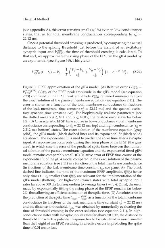
Figure 2: Evaluation of the gIF4 model. (A) Comparison of excitatory (top) andinhibitory (bottom) postsynaptic potentials (PSPs) in the gIF4 model (black solidlines; see equation 2.16) and the exact solution of the original differential equa-tion, 2.11 (see gray solid lines). Traces are shown for different offset membranepotentials V0, ranging from the leak reversal VL to the firing threshold Vthres, aswell as for three different total membrane conductances expressed in terms ofmultiples of the leak membrane time constant, τ L
m = 22.12 ms. Model parametersfor the simulations are identical to those used in Rudolph and Destexhe (2006)and are given in appendix A. (B) Relative error (V(t) − VgIF4(t))/(V(t) − Vthres)
between the exact solution of the PSP time course in the leaky IF model (V(t),equation 2.3) and the gIF4 model (VgIF4(t)) at firing threshold as a function oftime after excitatory (dashed) and inhibitory (solid) synaptic inputs. Results areshown for the three total membrane conductances used in panel A. In all cases,the error was smaller than 1% for times covering the PSP peak (gray area; see in-set). (C) Example of a membrane potential time course resulting from a barrageof synaptic inputs. The piecewise exact solution of equation 2.3 (gray) given inequation 2.11 is compared with the gIF4 model (black) for an identical synapticinput pattern (total input rate of about 10 kHz) 10,000 seconds after start of thecorresponding simulation. Both the subthreshold dynamics (bottom) and spik-ing response (top) are reproduced with high precision, although occasionallyspikes are omitted (solid triangles) or slightly delayed (open triangles).

1442 M. Rudolph-Lilith, M. Dubois, and A. Destexhe
A
C
B
1 0.2 0.1
2
4
6
8
x Δτ
me
x τmL
1
2
3
%
0 4 8
40
20
%
0 2 4t-t (ms)0
5
10
15
0.06 0.12distance to threshold (mV)
0.04
0.08
ms
0.05 mV
2 ms
Vthres
tnumtexp
exact solution
gIF4 exponential fitgIF4
D 0.5
0.2x τ mL
0.1
0.5
0.2x τ mL
0.1
0.5
0.2x τ mL
0.1
where
A = �τ emτe
(1τ L
m+ 1
�τ em
) (V0 − VL
VL − Ve
(1τ L
m− 1
τe
)+ V0 − Ve
VL − Ve
1�τ e
m
).
The relative error in the estimation of the EPSP peak amplitude of thegIF4 model (see equation 2.23) compared to the peak amplitude obtainedfrom the numerical solution of the passive membrane equation is shown inFigure 3A. For biophysically reasonable values of the quantal conductance,expressed in terms of the associated quantal synaptic time constant �τ e
m
The gIF4 Method 1443
(see appendix A), this error remains small (�1%) even in low-conductancestates, that is, for total membrane conductances corresponding to τ L
m =22.12 ms.
Once a potential threshold crossing is predicted, by comparing the actualdistance to the spiking threshold just before the arrival of an excitatorysynaptic input and Vmax
EPSP, the time of threshold crossing is calculated. Tothat end, we approximate the rising phase of the EPSP in the gIF4 model byan exponential (see Figure 3B). This yields
VexpEPSP(t − t0) = V0 − 1
T
(V0 − VL
τ Lm
+ V0 − Ve
τ em
) (1 − e−T(t−t0 )
), (2.24)
Figure 3: EPSP approximation of the gIF4 model. (A) Relative error (VmaxEPSP −
Vmax(gIF4)
EPSP )/VmaxEPSP of the EPSP peak amplitude in the gIF4 model (see equation
2.23) compared to the EPSP peak amplitude VmaxEPSP obtained numerically from
the exact solution of the passive membrane equation (see equation 2.11). Theerror is shown as a function of the total membrane conductance (in fractionsof the leak membrane time constant τ L
m = 22.12 ms) and the quantal excita-tory synaptic time constant �τ e
m. For biophysically realistic parameters (seethe dotted area) ×�τ e
m ≈ 1 and ×τ Lm ≈ 0.2, the relative error stays far below
1%. (B) Characteristic EPSP time course in low-conductance (total membraneconductance corresponding to τ L
m = 22.12 ms; top) and high-conductance (τ Lm =
2.212 ms; bottom) states. The exact solution of the membrane equation (graysolid), the gIF4 model (black dashed line) and its exponential fit (black solid)are shown. The exponential fit is used to predict the spike time after a synapticinput. A response can occur only during the rising phase of the EPSP (the grayarea), in which case the error of the predicted spike times between the numeri-cal solution of the passive membrane equation and the exponential fitted gIF4model remains comparably small. (C) Relative error of EPSP time course of theexponential fit of the gIF4 model compared to the exact solution of the passivemembrane equation (see 2.11) as a function of the total membrane conductance(in fractions of the leak membrane time constant τ L
m, see panel A). The blackdashed line indicates the time of the maximum EPSP amplitude, tmax
EPSP; henceonly times t − t0 smaller than tmax
EPSP are relevant for the implementation of thegIF4 model (bottom). For high-conductance states with total synaptic inputrates far above 500 Hz (corresponding to average times t − t0 � 2 ms), the errormade by exponentially fitting the rising phase of the EPSP remains far below2%, thus allowing an efficient estimation of the spike time. (D) Absolute error inthe prediction of the spike time tspike − t(exp)
spike as a function of the total membraneconductance (in fractions of the leak membrane time constant τ L
m = 22.12 ms)and the distance to threshold. tspike was obtained by numerically evaluating thetime of threshold crossing in the exact solution (see equation 2.11). In high-conductance states with synaptic inputs rates far above 500 Hz, the distance tothreshold for which a potential response has to be calculated is much smallerthan the height of an EPSP, resulting in effective errors in predicting the spiketime of 0.01 ms or less.

1444 M. Rudolph-Lilith, M. Dubois, and A. Destexhe
where
T = 1τ L
m+ 1
τ em
+ τ Lm
τe
VL − Ve
(V0 − VL)τ em + (V0 − Ve)τ
Lm
.
Although the error made by this approximation increases rapidly after thesynaptic input (see Figure 3C, top), it remains below 5% for up to 2 msafter the input (corresponding to average input rates above 500 Hz), andapproaches zero if high-conductance states with realistic total input ratesabove 10 kHz are considered.
With equation 2.24, it is now possible to estimate the potential spike timein response to a threshold-crossing excitatory synaptic input. Assuming afixed threshold Vthresh, we obtain
tspike = − 1T
log[
1 + T(Vthres − V0)τ
Lmτ e
m
(V0 − VL)τ em + (V0 − Ve)τ
Lm
](2.25)
for the future spike time. The closer the membrane potential before the ar-rival of the synaptic input (V0) resides to the threshold Vthres, the smaller isthe error in the predicted response time. In high-conductance states with ahigh average input rate, V0 will be very close to the threshold, resulting inspike time prediction errors of less than 0.01 ms (see Figure 3D). However,this relatively small error is somewhat misleading as the gIF4 model (seeequation 2.17) provides only an approximation of the true membrane statetime course in response to a synaptic bombardment. Thus, it is expectedthat small numerical errors will accumulate and yield a membrane statetime course that will increasingly deviate from its true course and, hence,lead to a deviation of the spiking response due to the approximation ofthe subthreshold behavior. However, as we show in section 3, these devi-ations remain small if low-order statistical measures of the response areconsidered, and they even remain negligible at the statistical level ininherently noisy neural systems in which spike timing plays an importantrole.
2.4 An Event-Driven Implementation of the gIF4 Neuron Model. Be-fore evaluating the response of the gIF4 neuron model in comparisonwith the numerical solution of the original passive membrane equationwith conductance-based synaptic interactions, we present in this sectiona basic event-driven implementation of the proposed model. In Rudolphand Destexhe (2006), we briefly outlined the advantages and disadvan-tages of event-driven simulation strategies over the still most widely usedclock-driven frameworks (for more details, see also Brette, 2006; Brette et al.,2007). In its most efficient implementation, an event-driven simulation strat-egy makes use of an analytic form of the state equations describing the

The gIF4 Method 1445
evolution of the membrane state variables in between the arrival of synap-tic inputs. This way, the sole knowledge of the membrane state at the lastsynaptic event, along with the time difference, is sufficient to calculate andupdate the state variables at the arrival time of a new synaptic input. Thisallows the neural simulation to “jump” from event to event rather than toevaluate the membrane state variables on a fixed temporal grid, as used insynchronous or clock-driven simulation strategies, thus rendering the com-putational efficiency of event-driven strategies dependent on the activity inthe model itself.
The proposed gIF4 model is analytically closed (see equations 2.16 and2.17) and, hence, allows an efficient implementation within the event-drivencontext in a similar fashion as that used for the previous gIF models (seesection 4 in Rudolph & Destexhe, 2006). However, as in the previousgIF models, the gIF4 model will not provide an exact (up to the chosenmachine precision) solution, in contrast to the general advantage of event-driven simulation strategies. Although spike times are computed analyti-cally (see equation 2.25) and utilized at machine precision, the approxima-tive nature of the gIF4 model will inherently diminish the precision of thesimulation.
Moreover, due to the delay between synaptic input and potential re-sponse, the treatment of response spikes requires more care than in theprevious models. Here we present a basic incorporation of the gIF4 modelinto the NEURON simulation environment (Hines & Carnevale, 1997, 2004).(Models are available online at http://cns.iaf.cnrs-gif.fr/. ) In the proposedimplementation, the following steps are executed on the arrival of a newsynaptic event at time t1 after a preceding input at time t0:
Step 1. At the arrival of a synaptic event, independent of the current stateof the membrane, the actual membrane time constant τm(t1) and itssynaptic contributions τ
{e,i}m (t1) are calculated using equation 2.18,
with the values of the synaptic contributions to the membrane timeconstant τ
{e,i}m (t1) (see equation 2.20) and values for τ
{e,i}m (t0) after the
previous synaptic event at time t0.Step 2. If the neuron is not in its refractory period, the state variable V(t1)
is calculated using equation 2.17, in which t0 denotes the time of theprevious synaptic event, V(t0) is the membrane state, and τ
{e,i}m (t0)
are the excitatory and inhibitory synaptic contribution to the totalmembrane time constant at time t0. If the neuron is in the refractoryperiod, then V(t1) = Vrest , and the model waits for next synaptic input(step 1).
Step 3. For excitatatory synaptic input, the maximum EPSP amplitude iscalculated (see equation 2.23). If V0 + Vmax
EPSP > Vthres, the spike time ispredicted (step 4). Otherwise the model waits for the next synapticinput (step 1). For inhibitory synaptic input, the model waits for thenext synaptic input (step 1).
1446 M. Rudolph-Lilith, M. Dubois, and A. Destexhe
Step 4. The spike time is calculated according to equation 2.25. If a spikein response to the synaptic input at t0 was already calculated, replacethe predicted spike time with the newly calculated one.
If the predicted spike time tspike < t1, a spike is generated and the cellenters an absolute refractory period after which the state variable is reset toits resting value Vrest. The spike event is added to an internal event list andcauses, after a transmission delay, a synaptic event in target neurons.
3 Response Dynamics of the gIF4 Model
In this section, we briefly compare the spiking response dynamics of thegIF4 model to that of the passive membrane equation with exponentialCOBA synapses and fixed spike threshold solved numerically. To allowcomparison with the previous gIF models, we used the same tests as in theoriginal study (Rudolph & Destexhe, 2006). In the following section, we firstcharacterize the statistics of spontaneous discharge activity. In section 3.2,we study the temporal resolution of synaptic inputs in the different mod-els. Finally, in section 3.3 we investigate the modulatory effect of synapticinputs on the cellular gain. Computational models and model parametersare outlined in appendix A.
3.1 Spontaneous Discharge Statistics. A spontaneous discharge in theinvestigated models was evoked by Poisson-distributed random release atsingle independent synaptic input channels for excitation and inhibitionwith stationary rates covering a physiologically relevant parameter regime(see appendix A). Total input rates ranged from νi = 0 to 30 kHz for inhibi-tion and νe = 0 to 100 kHz for excitation.
As expected, the cell’s output rate νout increased with increasing νe andreached beyond 300 Hz for an extreme excitatory drive (see Figure 4A).Moreover, in the investigated input parameter regime, a nearly linear re-lationship between excitatory and inhibitory synaptic release rates wasobserved. Although the gIF4 model and the numerical simulation of thepassive membrane equation exhibited nearly identical qualitiative andquantitative behaviors, the slope of the equi-νout lines was slightly higherfor the gIF4 model, suggesting a stronger dependency on the excitatorydrive of the approximated analytical solution. The reason for this behav-ior can be found in the fact that the PSP time course in the gIF4 modelslightly deviates from that of the full numerical solution (see Figure 2B). Thiserror accumulates for each PSP and, hence, increases with increasing inputrate. As the excitatory rate was about three times larger than the inhibitorydrive, a stronger dependency of the output rate on the excitatory drive isexpected.
The quality of the gIF4 approximation was further probed by evaluatingthe coefficient of variation CV in the investigated parameter regime. The CV

The gIF4 Method 1447
A
B
20
ν (
kHz)
i
10
ν (kHz)e
30 60 90
20
ν (
kHz)
i
10
ν (kHz)e
30 60 90
200 20
ν (
kHz)
i
10
ν (kHz)e
30 60 90
ν (Hz)out
100
20
ν (
kHz)
i
10
ν (kHz)e
30 60 90
CV
1
0.6
0.2
PMEgIF4
Figure 4: Spontaneous discharge rate (A) and coefficient of variation CV (B) asa function of the total frequency of inhibitory and excitatory synaptic inputs.The gIF4 model (left) is compared with the numerical solution of the passivemembrane equation (PME; right). The CV is defined as CV = σISI/ISI, where σISI
denotes the standard deviation of the interspike intervals and ISI the meaninterspike interval. The input for both models consisted of two independentinput channels for excitation and inhibition releasing at rates between 0 and100 kHz (for excitation) and 0 and 30 kHz (for inhibition). The parameters ofsynaptic kinetics and the time course of synaptic conductances are given inappendix A.
is defined by
CV = σISI
ISI, (3.1)
where σISI denotes the standard deviation of the interspike intervals (ISIs)and ISI the mean ISI. For both models, a qualitiatively and quantitatively

1448 M. Rudolph-Lilith, M. Dubois, and A. Destexhe
similar behavior was found (see Figure 4B), with slight differences in theslope of equi-CV lines explainable by differences in the firing rate as afunction of the excitatory and inhibitory input rates (see Figure 4A). In theinvestigated parameter regime, CV values reaching up to 1.2 were observed.In general, higher firing rates led to a more regular discharge (i.e., smallerCV values), with only a narrow band with intermediate firing rates and bal-anced excitation and inhibition displaying higher coefficients of variations.
Finally, in order to test whether the high irregularity in the spontaneousdischarge stems from a Poisson process (Smith & Smith, 1965; Noda, Adey,1970; Burns & Webb, 1976; Softky & Koch, 1993; Stevens & Zador, 1998b),we investigated the distribution and autocorrelation of interspike intervals(ISIs). In input regimes yielding high irregularity (CV around 1) at phys-iologically relevant firing rates for in vivo activity (around 10 to 20 Hz;see Evarts, 1964; Steriade & McCarley, 1990), we found that ISI histogramsshowed pronounced peaks at small ISIs and were in general not fittablewith a gamma distribution (see Figure 5A), thus deviating from the dis-tribution expected from a Poisson process. Moreover, in both models, theautocorrelograms displayed small peaks at small lag times (see Figure 5B),indicating that subsequent output spikes were not independent. These devi-ations from a spontaneous discharge that is both independent and Poissondistributed indicate the limitations of a fixed threshold spike-generatingmechanism to reproduce realistic discharge statistics. However, both thePME and gIF4 model showed remarkable agreement in their statistical be-havior, suggesting that the approximation of the gIF4 model reproduceswith high precision the spontaneous discharge statistics observed in thepassive membrane equation with synaptic conductances and fixed spikingthreshold.
3.2 Temporal Resolution of Synaptic Inputs. In a second comparativetest of the behavior of the gIF4 model, we investigated the ability of themodel to resolve a periodic weak synaptic stimulation (coactivation of 10–40 synapses), superimposed on an intense but fixed background activity.The frequency of the periodic stimulus νstim was varied in successive trialsbetween 5 and 200 Hz, corresponding to interstimulus intervals Tstim rang-ing from 200 to 5 ms, respectively. This periodic stimulus appears in theinterspike interval histogram (ISIH) as peak at or close to the frequency ofthe stimulus (see Figure 6A, inset and 6B). The latter can be used to definethe temporal resolution (Destexhe et al., 2003),
Temporal resolution = Tstim
TISI, (3.2)
where Tstim denotes the period of the periodic stimulus and TISI the positionof the stimulus-induced peak in the ISIH. Due to limitations in the temporal

The gIF4 Method 1449
PMEgIF4
ISI (ms) 100 200
ISI d
ensi
ty (1
/ms)
0.1
0.2
ISI (ms) 100 200
Lag Time (ms) 50 150
ρ (1
0 /
ms)
-3
0.4
0.8
100
0.6
0.2
Lag Time (ms) 50 150 100
A
B
Figure 5: Typical interspike interval histograms (ISIH; A) and autocorrelograms(B) for the gIF4 model (left) and the numerical solution of the passive membraneequation (PME; right). Synaptic input rates were chosen to yield comparableoutput rates at high CV values (CV = 0.96 for PME and 0.91 for gIF4), and a five-fold decrease in input resistance compared to the quiescent case (see appendixA). ISIHs were fitted with gamma distributions ρISI(T ) = 1
q! ar(rT )q e−rT , whereρISI(T ) denotes the probability for occurrence of ISIs of length T and r, a, andq are parameters. Fitted parameters are q = 1, r = 0.042 ms−1, a = 0.824 (PME)and q = 1, r = 0.039 ms−1, a = 0.879 (gIF4).
resolution capability of the membrane and the related low-pass filtering ofsynaptic inputs, TISI will in general be larger than TISI, especially for high-frequency stimuli. Thus, equation 3.2 measures the “deviation” from theideal situation, for which the stimulus would lead to a sharp peak in theISIH at TISI = Tstim.
The results show that both models are able to resolve the periodic stim-ulus faithfully up to 100 Hz. Moreover, both models show a remarkablysimilar response in both the output rate νout (see Figure 6A, left) and tem-poral resolution (right panel) up to a stimulation frequency of 100 Hz
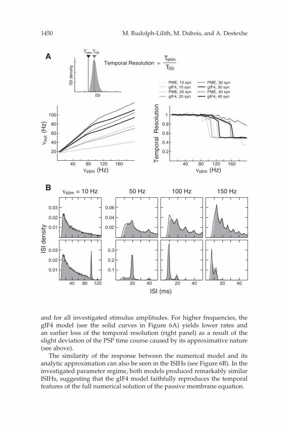
1450 M. Rudolph-Lilith, M. Dubois, and A. Destexhe
ISI
ed ISI
ytisn
TstimTISI
Tstim
TISITemporal Resolution =
40 80 120 160
20
60
100
40
80
ν (Hz)stim
ν)z
H(tuo
40 80 120 160ν (Hz)stim
0.2
0.6
1
0.4
0.8
eT
noituloseR larop
m
A
B
gIF4, 40 synPME, 40 syngIF4, 30 synPME, 30 synPME, 10 syn
gIF4, 20 synPME, 20 syngIF4, 10 syn
ν = 10 Hzstim 50 Hz 100 Hz 150 Hz
ISI (ms)40 80 120
ytisned ISI
0.01
0.03
0.02
0.01
0.03
0.02
0.02
0.06
0.04
0.1
0.3
0.2
20 40 20 40 20 40
and for all investigated stimulus amplitudes. For higher frequencies, thegIF4 model (see the solid curves in Figure 6A) yields lower rates andan earlier loss of the temporal resolution (right panel) as a result of theslight deviation of the PSP time course caused by its approximative nature(see above).
The similarity of the response between the numerical model and itsanalytic approximation can also be seen in the ISIHs (see Figure 6B). In theinvestigated parameter regime, both models produced remarkably similarISIHs, suggesting that the gIF4 model faithfully reproduces the temporalfeatures of the full numerical solution of the passive membrane equation.

The gIF4 Method 1451
3.3 Gain Modulation. Finally, we tested both models’ ability to capturethe modulatory effect of synaptic background activity on the response gain.To that end, we stimulated the cells periodically with 0 to 50 simultaneouslyreleasing excitatory synapses and modulated the synaptic background ac-tivity by scaling the frequency of excitatory and inhibitory inputs between0.5 and 2.0 around a set of default values (see the caption to Figure 6). Thebehavior was then characterized by the probability of emitting a spike as afunction of the given stimulus, which typically shows a sigmoidal shape. Byfitting the numerical results with a sigmoidal function (see Figure 7, inset),we obtained the slope (“Slope” in Figure 7) and the stimulation amplitudefor which the response probability takes 50% (“Mid Amplitude” in Fig-ure 7). Both measures were then used to characterize the gain modulatorybehavior of the investigated neuronal models.
The numerical model (PME) reproduced the behavior already seen inthe original study (Rudolph & Destexhe, 2006), with synaptic backgroundactivity being efficient in modulating the cellular response, in particular theresponse gain (see Figure 7, top right). As expected, the slope decreasedfor increasing background activity, suggesting a more graded response forhigher background activity (see Figure 7, bottom right). The mid-amplitudeshowed a minimum for intermediate background activity—the stimulationamplitude required to yield a response was optimal in a limited regime ofnonvanishing background noise (see Figure 7, bottom left). This behaviorresembles closely that of the stochastic resonance phenomenon, in which adynamic system displays a more optimal response for intermediate noiselevels.
Figure 6: Temporal resolution of periodic synaptic inputs in the presence ofbackground activity. (A) Total output rate νout (left) and temporal resolution(right; see the inset for definition) in models (PME: numerical solution of thefull membrane equation; gIF4: gIF4 model) driven by Poisson synaptic inputsas well as periodic stimuli of frequency νstim between 5 Hz and 200 Hz andamplitudes corresponding to the simultaneous activation of 10 to 40 synapses.Both models show a remarkably similar qualitative and quantitative response,in particular for stimulation rates below 100 Hz. Moreover, both models are ableto resolve the periodic stimulus faithfully up to 100 Hz (temporal resolution ∼1; right panel). (B) Typical ISIHs for both models (PME: black solid line; gIF4:gray shading) at different rates of the periodic stimulus νstim, for stimulation am-plitudes of 10 (top) and 40 (bottom) synapses. The gIF4 model reproduces withhigh accuracy the ISIHs of the numerical solution of the passive membraneequation, while requiring a much lower computational load. Parameters: Tocompare the behavior for similar output rates, the Poisson background activityfor both models was adjusted to yield the same output rate without additionalperiodic stimulus. The corresponding Poisson frequencies were 27.25 kHz (ex-citation) and 9.6 kHz (inhibition) for the PME model and 28 kHz (excitation)and 9.6 kHz (inhibition) for the gIF4 model. All other parameters were identical.

1452 M. Rudolph-Lilith, M. Dubois, and A. Destexhe
ytilibaborP
Stimulation Amplitude
Mid Amplitude
Slope
SimulationSigmoidal Fit
0.6 1.4
20
60
SBA Scaling
edutilpm
A diM
40
1.0 1.8
epolS
0.6 1.4
SBA Scaling1.0 1.8
0.01
0.02
0.03
20
60
diM
ilpm
A dut
e
40
Slope0.01 0.02 0.03
PMEgIF4
Figure 7: Modulation of the neural response (gain modulation) through back-ground activity. The response probability ρ(gstim) as a function of the stimula-tion amplitude (inset top left; gray solid line) was fit with a sigmoidal function(black solid line) ρ(gstim) = (1 − exp(−agstim))/(1 + b exp(−agstim)), where a andb are free parameters and gstim denotes the stimulation amplitude. From thesefits, the stimulation amplitude (number of simultaneously releasing excitatorysynapses) yielding a probability of 50% (“Mid Amplitude”) and the slope wereestimated and plotted against each other for different levels of synaptic back-ground activity (top right) and as functions of the synaptic background activity(bottom) for the numerical solution of the passive membrane equation (graysolid line) and its analytical gIF4 approximation (black solid line). In both cases,the synaptic background activity was changed by applying a common scalingfactor (“SBA Scaling”), ranging from 0.5 to 2.0, to the frequency of excitatoryand inhibitory synaptic inputs given Figure 6. The number of simultaneouslyreleasing excitatory synapses ranged from 0 to 50.
Most importantly, the analytical approximation (gIF4) showed a behav-ior that very closely matched that of the full numerical solution of thepassive membrane equation. Differences were observed only at higher back-ground activity levels, at which the small error in the analytic approximationaccumulates more strongly.

The gIF4 Method 1453
3.4 Performance Evaluation. The analytically closed form of the gIF4model is expected to be advantageous for the computational load whencompared to the numerical solution of the original passive membrane equa-tion. In order to investigate this issue in more detail, we analyzed the perfor-mance of both models with respect to numerical precision and the resultingcomputational load.
To that end, we first simulated neural activity for identical synaptic inputdrive and evaluated the superthreshold and subthreshold response aftera sufficiently long period of simulated activity. Typical traces are shownin Figures 8A and 8C. The numerical solution of the passive membraneequation (see “PME,” Figure 8A) using the classical fourth order Runge-Kutta method at various integration time constants ranging from dt = 0.5 msto 0.0001 ms yields a numerically converging activity pattern for decreasingintegration time constants dt, hence increasing precision of the numericalintegrator. The membrane potential time course was found to be practicallyidentical for dt below 0.01 ms (see Figure 8C), and spikes were emitted attimes that varied with the order of the used fixed integration time step.
Defining the resulting spike pattern obtained for the highest investigatedtemporal resolution (see “PME” 0.0001 ms, Figure 8A) as the “expectedsolution,” we observed a qualitative and quantitative change for integrationtime constants above 0.01 ms. Not just deviated individual spike timesfrom the expected solution, but above dt ≈ 0.1 ms, significant deviationsin lowest-order spike statistics (such as the average rate) were observed.In contrast, the event-driven simulation of the gIF4 model displayed asuprathreshold (see “gIF4,” Figure 8A) and subthreshold behavior (seeFigure 8A) which matched to a high degree of numerical accuracy theexpected solution. We note, however, that the fourth-order Runge-Kuttamethod can also be applied in an event-driven framework by numericallysolving the differential equation only at times of arriving synaptic inputs. Inthis case, the solution is expected to converge directly to the true value, witha numerical precision that will likely be superior to that of the approximatedgIF4 model (not shown).
To evaluate the computational load accompanying the numerical simula-tion, we next recorded the time needed to simulate 1000 s of neural activity.To allow comparison with the gIF1 to three models, we followed the samestrategy for performance evaluation as introduced in our previous study(Rudolph & Destexhe, 2006). All models were implemented in the NEU-RON simulation environment (Hines & Carnevale, 1997, 2004), runningon the same hardware platform (a 3 GHz Dell Precision 350 workstation).Synaptic inputs were chosen to be Poisson distributed with a rate between4 and 80 kHz for the excitatory and between 1 and 20 kHz for the inhibitorychannel. Both rates were varied proportionally, such that the total averagerate took values between 5 and 100 kHz. As shown in Rudolph and Des-texhe (2006), the performance ratio was found to be mostly independent of
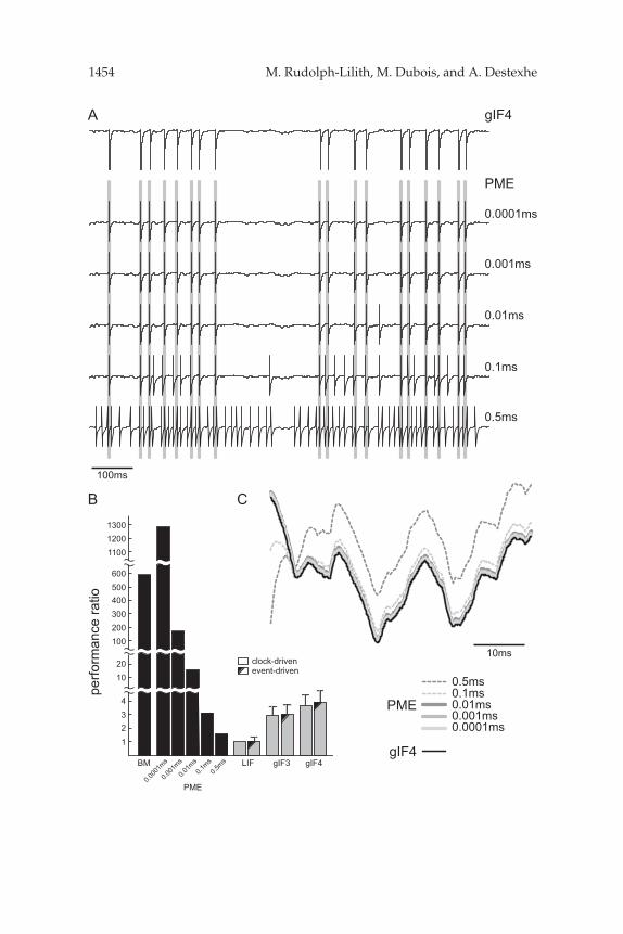
1454 M. Rudolph-Lilith, M. Dubois, and A. Destexhe
perfo
rman
ce ra
tio
LIF gIF3 gIF4
event-drivenclock-driven
1
234
1020
BM
100200
PME0.0
001m
s
0.001
ms
0.01m
s0.5
ms0.1
ms
300400500600
110012001300
100ms
gIF4
PME
0.0001ms
0.001ms
0.01ms
0.5ms
0.1ms
10ms
0.0001ms0.001ms0.01ms
0.5ms0.1ms
gIF4
PME
A
B C

The gIF4 Method 1455
the total synaptic input rate (see Figure 11C in Rudolph & Destexhe, 2006)in the investigated parameter regime, thus expressing the relative com-putational load in terms of a single number. Finally, synaptic and cellularproperties for both models were adjusted to give similar output rates (seethe caption to Figure 6).
As the analytical form of the gIF4 model is very similar to that of theprevious gIF1 to gIF3 models, a similar performance concerning compu-tational load is expected. Indeed, the gIF4 model performed only slightlyslower than the gIF3 model (see Figure 8B), which is attributable to the factthat in the former, the spike time has to be calculated in case the membraneis close to the spiking threshold. However, despite this slight decreasein computational efficiency, the NEURON implementation of the gIF4model still remains at least four times faster than the numerical solutionof the original passive membrane equation when solved by numericalintegration with an integration time constant of 0.01 ms. As outlined above,the latter must be viewed as an upper bound for the integration timeconstant in order to achieve an acceptable degree of accuracy (comparedto the expected solution) when solving the passive membrane equationwith (classical) Runge-Kutta in a clock-driven framework. Finally, thegIF4 model was found to be more than two orders of magnitude moreefficient than the full biophysical model with Hodgkin-Huxley spikegeneration while at the same time displaying a dynamics comparable tothese biophysically more realistic models.
We note that the rather crude performance evaluation does not reflectthe potentially achievable performance gain of the gIF4 model. Preliminaryevaluations done within a customized simulation environment written inANSI C and optimized assembly routines showed that event-driven im-plementations of the classical IF can yield performance gains of more thanone order of magnitude compared to the NEURON implementation of thesame model or the clock-driven implementation of the passive membrane
Figure 8: Performance evaluation. (A) Typical examples of the membrane po-tential time course for identical synaptic drive (Poisson inputs with 28 kHz forexcitation and 9.6 kHz for inhibition and identical random seed) after 10,000s simulated activity for the gIF4 model (top trace) and the passive membraneequation (PME) solved numerically using classical the fourth-order Runge-Kutta method at different time resolutions between 0.0001 ms and 0.5 ms.The gray bars indicate spikes occurring for PME at 0.0001 ms time resolution.(B) Comparison between the performance, normalized to the clock-driven sim-ulation of the leaky IF neuron model (PME: 1287 (0.0001 ms), 138.5 (0.001 ms),15.65 (0.01 ms), 3.24 (0.1 ms), 1.52 (0.5 ms); gIF4, clock-driven: 3.72 ± 0.82,event-driven: 3.93 ± 0.89). See the text for details. (C) Examples of subthresholdactivity for identical synaptic input drive (see panel A) for the gIF4 model andthe passive membrane equation (PME).

1456 M. Rudolph-Lilith, M. Dubois, and A. Destexhe
equation (not shown). Moreover, the analytical form of the gIF4 modelis given in terms of exponential functions alone, for which most moderncomputational hardware is optimized. Comparing the gIF4 model with themodel introduced by Brette (2006, 2007), which requires the numerical eval-uation of gamma functions, the gIF4 models reach a performance gain ofat least one order of magnitude due to the computational load assigned tothe calculation of gamma functions. As the arguments of the exponentialfunctions in the gIF4 model are bound, an even more efficient implementa-tion in terms of linear machine-precision lookup tables can be envisioned,which was found to yield further performance gain in excess of three ordersof magnitude.
Finally, in our customized simulation environment, we found that onlyabout 2% of the total simulation time is used for updating the state vari-ables (compared to more than 10% in NEURON), whereas the remaining98% account for the generation of random numbers for synaptic inputs.Replacing the random number generation by more optimized algorithmsor hardware-generated random numbers, a further performance improve-ment of at least a factor of 50 can be achieved, a factor that will also applyto the presented gIF4 model. Thus, utilizing modern hardware and effi-cient implementation, the real-time simulation of medium-scale neuronalnetworks of a few tens of thousands of neurons with biophysically morerealistic conductance-based synaptic interactions becomes possible on astandard desktop computer.
4 Discussion
In Rudolph and Destexhe (2006), we proposed various models (the gIF1,gIF2, and gIF3 models) of analytical IF neurons with conductance-basedsynaptic dynamics. These models are based on an analytical approxima-tion of the differential equation describing the IF neuron with exponentialsynaptic conductances and were successfully tested with respect to theirresponse to random and oscillating inputs. The driving idea behind devel-oping such simplified neuronal models by approximating the membraneequation was to provide analytically solvable models for use in fast neu-ronal simulations using the event-driven simulation strategy.
Due to their simple mathematical structure, the gIF models are bestsuited for fast event-driven simulation strategies. However, the approxi-mations in the original gIF models were based on the assumption of an in-stantaneous rise and exponential decay of the postsynaptic potential (PSP).This limitation might have an impact in situations where the exact timing ofpre- and postsynaptic events is of importance, such as in models of spike-timing-dependent plasticity. In this letter, we addressed this limitation byconceiving an analytical approximation of the COBA IF neuron model withthe full PSP time course and an analytical prediction of the postsynapticresponse time.

The gIF4 Method 1457
The subthreshold and suprathreshold response of this gIF4 model to var-ious synaptic input paradigms reproduces remarkably well the correspond-ing responses of the passive membrane equation subjected to conductancenoise solved numerically, while gaining significant performance in com-parison to the latter. Although the analytical structure of the gIF4 modelis more complex than that of the previously introduced models due to theneed to calculate future spike times, a simple and algorithmically efficientimplementation for use in large-scale neural simulations was proposed, to-gether with a basic evaluation of the possibility of modeling medium-sizednetworks in real-time.
The presented gIF4 model, as well the gIF models in our previous study(Rudolph & Destexhe, 2006), should not be viewed as a model of an iso-lated single cells but rather as a building block of a large interconnectedneural network. Specifically, the proposed models cannot simulate artifi-cially induced responses such as periodic firing following constant currentor conductance injection. Instead, as the update of the state variable is solelytriggered by the arrival of (excitatory) synaptic conductances, the proposedmodels’ applicability focuses on their use in large-scale neural networkswith conductance-based synaptic interactions.
Future investigations and extensions of this new model will be made intwo directions. First, so far, no mechanism for adaptation, bursting, or a vari-able spiking threshold, which would reflect more precisely biophysical real-ity, has been introduced into the model. However, due to the fact that manypeculiarities of the biophysical cellular dynamics can be captured by ex-tending the passive membrane equation with additive terms linear in theirdependence on the state variable, these extensions should remain a straight-forward exercise. Second, and more important, the proposed model remainsto be evaluated in both efficiency and precision at the network level. To thatend, we are currently developing a high-performance neural simulationenvironment (CYLon-1, CYDYNS Technologies, http://www.cydyns.com)for simulating large-scale neural networks of hundreds of thousand neu-rons in real time using the event-driven framework. The most challengingtask for the future is to evaluate and understand in vivo–like neuronal dy-namics in such large-scale systems, in particular with a view on the emer-gence of specific functional behaviors when endowed with self-organizingcapabilities.
Appendix: Computational Models and Methods
In this appendix, we briefly describe the IF model based on the passivemembrane equation and fixed threshold for spike generation (PME), andsummarize the parameters used for numerical simulations.
In what we refer to as the passive membrane equation with fixedspike threshold (PME), membrane dynamics was simulated using a
1458 M. Rudolph-Lilith, M. Dubois, and A. Destexhe
single-compartment neuron, described by the passive membrane equation
dV(t)dt
= − 1τ L
m
(V(t) − VL
) − 1C
Isyn(t). (A.1)
Here, V(t) denotes the membrane potential, VL = −80 mV the leak reversalpotential, τ L
m = C/GL the membrane time constant, C = aCm the membranecapacity (specific membrane capacity Cm = 1 μF cm−2, membrane area a =38,013 μm), and GL = agL the passive (leak) conductance (leak conductancedensity gL = 0.0452 mS cm−2, corresponding to a passive leak membranetime constant of τ L
m = 22.12 ms). Spike generation was described by a fixedvoltage threshold (Vthres = −50 mV) and reset potential (Vrest = −80 mV).The refractory period in all cases was tre f = 1 ms.
Simulations of 1000 s neural activity with a fixed temporal resolutionof 0.01 ms were performed using the NEURON simulation environment(Hines & Carnevale, 1997), running on a 3 GHz Dell Precision 350 work-station under the SUSE 8.1 LINUX operating system. NEURON models aremade available online at http://cns.iaf.cnrs-gif.fr/.
The gIF4 neuronal model was solved using equation 2.17 with the samecellular parameters.
Synaptic inputs were simulated by exponential conductance (or timeconstant) changes with the following parameters: �τ e
m = 575.96 ms, τe = 2ms for excitatory conductances, �τ i
m = 601.3 ms, τi = 10 ms for inhibitoryconductances. Due to the additivity of synaptic inputs for this case, inall models synaptic inputs were simulated by single independent inputchannels for excitation and inhibition, with total rates of 0 ≤ νe ≤ 100 kHzand 0 ≤ νi ≤ 30 kHz, respectively.
To evaluate the computational performance of the constructed models,simulations utilizing the clock-driven simulation strategy (time resolution0.01 ms), as well as the event-driven simulation strategy (Watts, 1994; Mat-tia & Del Giudice, 2000; Reutimann et al., 2003), were used. In all cases,simulation of 1000 s neural activity were performed.
In some simulations, we used a novel, high-performance gen-eral graph simulation environment CYLon-1 (CYDYNS Technologies,http://www.cydyns.com). This environment is optimized for, but not re-stricted to, event-driven simulation strategies and uses a software architec-ture that allows its use on a variety of hardware platforms (shared-memorymulticore CPU/GPU systems, distributed cluster systems). This programis in beta development and will become available soon.
Acknowledgments
We thank Andrew Davison for stimulating discussions. This research wassupported by CNRS, HFSP, and the European Community (integratedproject FACETS, IST-15879 and BrainScales, IST-269921).

The gIF4 Method 1459
References
Abbott, L. F., & van Vreeswijk, C. (1993). Asynchronous states in networks of pulse-coupled oscillators. Phys. Rev. E, 48, 1483–1490.
Brette, R. (2006). Exact simulation of integrate-and-fire models with synaptic con-ductances. Neural Comput., 18, 2004–2027.
Brette, R. (2007). Exact simulation of integrate-and-fire models with exponentialcurrents. Neural Comput., 19, 2604–2609.
Brette, R., Rudolph, M., Carnevale, T., Hines, M., Beeman, D., Bower, J. M., et al.(2007). Simulation of networks of spiking neurons: A review of tools and strate-gies. J. Comput. Neurosci., 23, 349–398.
Burns, B. D., & Webb, A. C. (1976). The spontaneous activity of neurons in the cat’svisual cortex. Proc. R. Soc. London, B194, 211–223.
Carrillo, R. R., Ros, E., Tolu, S., Nieus, T., & D’Angelo, E. (2008). Event-driven simu-lation of cerebellar granule cells. Biosystems 94, 10–17.
Delorme, A., Gautrais, J., van Rullen, R., & Thorpe, S. (1999). SpikeNET: A simulatorfor modeling large networks of integrate and fire neurons. Neurocomputing, 26–27,989–996.
Delorme, A., & Thorpe, S. J. (2003). SpikeNET: An event-driven simulation packagefor modeling large networks of spiking neurons. Network: Comput. Neural Syst.,14, 613–627.
Destexhe, A., Rudolph, M., Fellous, J.-M., & Sejnowski, T. J. (2001). Fluctuating synap-tic conductances recreate in vivo–like activity in neocortical neurons. Neurosci.,107, 13–24.
Destexhe, A., Rudolph, M., & Pare, D. (2003). The high-conductance state of neocor-tical neurons in vivo. Nature Rev. Neurosci., 4, 739–751.
D’Haene, M., & Schrauwen, B. (2010). Fast and exact simulation methods appliedon a broad range of neuron models. Neural Comput., 22, 1468–1472.
D’Haene, M., Schrauwen, B., Van Campenhout, J., & Stroobandt, D. (2009). Accel-erating event-driven simulation of spiking neurons with multiple synaptic timeconstants. Neural Comput., 21, 1068–1099.
Evarts, E. V. (1964). Temporal patterns of discharge of pyramidal tract neurons duringsleep and waking in the monkey. J. Neurophysiol., 27, 152–171.
Fourcaud-Trocme, N., Hansel, D., van Vreeswijk, C., & Brunel, N. (2003). How spikegeneration mechanisms determine the neuronal response to fluctuating inputs.J. Neurosci., 23, 11628–11640.
Gerstner, W., & Kistler, W. M. (2002). Spiking neuron models. Cambridge: CambridgeUniversity Press.
Gerstner, W., Ritz, R., & van Hemmen, J. L. (1993). A biologically motivated andanalytically soluble model of collective oscillations in the cortex: I. Theory ofweak locking. Biol. Cybern., 68, 363–374.
Gerstner, W., & van Hemmen, J. L. (1992). Associative memory in a network of“spiking” neurons. Network, 3, 139–164.
Gerstner, W., & van Hemmen, J. L. (1993). Coherence and incoherence in a globallycoupled ensemble of pulse-emitting units. Phys. Rev. Lett., 71, 312–315.
Giugliano, M. (2000). Synthesis of generalized algorithms for the fast computation ofsynaptic conductances with Markov kinetic models in large network simulations.Neural Comput., 12, 903–931.

1460 M. Rudolph-Lilith, M. Dubois, and A. Destexhe
Giugliano, M., Bove, M., & Grattarola, M. (1999). Activity-driven computationalstrategies of a dynamically regulated integrate-and-fire model neuron. J. Comput.Neurosci., 7, 247–254.
Hansel, D., Mato, G., Meurier, C., & Neltner, L. (1998). On numerical simulations ofintegrate-and-fire neural networks. Neural Comput., 10, 467–483.
Hines, M. L., & Carnevale, N. T. (1997). The NEURON simulation environment.Neural Comput., 9, 1179–1209.
Hines, M. L., & Carnevale, N. T. (2004). Discrete event simulation in the NEURONenvironment. Neurocomputing, 58–60, 1117–1122.
Hodgkin, A. L., & Huxley, A. F. (1952). A quantitative description of membranecurrent and its application to conduction and excitation in nerve. J. Physiol., 117,500–544.
Izhikevich, E. M. (2001). Resonate-and-fire neurons. Neural Netw., 14, 883–894.Izhikevich, E. M. (2003). Simple model of spiking neurons. IEEE Trans. Neural Net-
works, 14, 1569–1572.Jolivet, R., Lewis, T. J., & Gerstner, W. (2004). Generalized integrate-and-fire models
of neuronal activity approximate spike trains of a detailed model to a high degreeof accuracy. J. Neurophysiol., 92, 959–976.
Knight, B. W. (1972). Dynamics of encoding in a population of neurons. J. Gen.Physiol., 59, 734–766.
Kuhn, A., Aertsen, A., & Rotter, S. (2004). Neuronal integration of synaptic input inthe fluctuation-driven regime. J. Neurosci., 24, 2345–2356.
Lansky, P., & Rospars, J. P. (1995). Ornstein-Uhlenbeck model neuron revisited. Biol.Cybern., 72, 397–406.
Lapicque, L. (1907). Recherches quantitatives sur l’excitation electrique des nerfstraitee comme une polarization. J. Physiol. Pathol. Gen., 9, 620–635.
LeMasson, G., Marder, E., & Abbott, L. F. (1993). Activity-dependent regulation ofconductances in model neurons. Science, 259, 1915–1917.
Markram, H., Wang, Y., & Tsodyks, M. (1998). Differential signaling via the sameaxon of neocortical pyramidal neurons. Proc. Natl. Acad. Sci. USA, 95, 5323–5328.
Mattia, M., & Del Giudice, P. (2000). Efficient event-driven simulation of large net-works of spiking neurons and dynamical synapses. Neural Comput., 12, 2305–2329.
Nicoll, A., Larkman, A., & Blakemore, C. (1993). Modulation of EPSP shape and ef-ficacy by intrinsic membrane conductances in rat neocortical pyramidal neuronsin vitro. J. Physiol., 468, 693–710.
Noda, H., & Adey, R. (1970). Firing variability in cat association cortex during sleepand wakefulness. Brain Res., 18, 513–526.
Reutimann, J., Giugliano, M., & Fusi, S. (2003). Event-driven simulations of spikingneurons with stochastic dynamics. Neural Comput., 15, 811–830.
Ricciardi, L. M., & Sacerdote, L. (1979). The Ornstein-Uhlenbeck process as a modelfor neuronal activity. I. Mean and variance of the firing time. Biol. Cybern., 35, 1–9.
Rudolph, M., & Destexhe, A. (2006). Analytical integrate-and-fire neuron modelswith conductance-based dynamics for event-driven simulation strategies. NeuralComput., 18, 2146–2210.
Rudolph, M., & Destexhe, A. (2007). How much can we trust neural simulationstrategies? Neurocomputing 70, 1966–1969.

The gIF4 Method 1461
Rudolph-Lilith, M., Dubois, M. & Destexhe, A. (2009) Analytical integrate-and-fireneuron models with conductance-based dynamics and realistic PSP time coursefor event-driven simulation strategies. In Eighteenth Annual Computational Neuro-science Meeting: CNS*2009 Meeting Abstracts, BMC Neuroscience 10 (Suppl. 1), P23.http://www.biomedcentral.com/1471-2202/10/S1/P23.
Senn, W., Markram, H., & Tsodyks, M. (2000). An algorithm for modifying neu-rotransmitter release probability based on pre- and postsynaptic spike timing.Neural Comput., 13, 35–67.
Smith, D. R., & Smith, G. K. (1965). A statistical analysis of the continuous activityof single cortical neurons in the cat unanesthetized isolated forebrain. Biophys. J.,5, 47–74.
Softky, W. R., & Koch, C. (1993). The highly irregular firing of cortical cells is incon-sistent with temporal integration of random EPSPs. J. Neurosci., 13, 334–350.
Steriade, M., & McCarley, R. W. (1990). Brainstem control of wakefulness and sleep. NewYork: Plenum.
Stevens, C. F., & Zador, A. M. (1998a). Novel integrate-and-fire-like model of repeti-tive firing in cortical neurons. In Proc. of the 5th Joint Symposium on Neural Comput.La Jolla, CA: UCSD.
Stevens, C. F., & Zador, A. M. (1998b). Input synchrony and the irregular firing ofcortical neurons. Nature Neurosci., 1, 210–217.
Stuart, G., & Spruston, N. (1998). Determinants of voltage attenuation in neocorticalpyramidal neuron dendrites. J. Neurosci., 18, 3501–3510.
Tonnelier, A., Belmabrouk, H., & Martinez, D. (2007). Event-driven simulations ofnonlinear integrate-and-fire neurons. Neural Comput., 19, 3226–3238.
Tsodyks, M., Mit’kov, I., & Sompolinsky, H. (1993). Pattern of synchrony in inho-mogeneous networks of oscillators with pulse interaction. Phys. Rev. Lett., 71,1280.
Watts, L. (1994). Event-driven simulations of networks of spiking neurons. In J. D.Cowan, G. Tesauro, & J. Alspector (Eds.), Advances in neural information processingsystems, 6 (pp. 927–934). San Mateo, CA: Morgan Kaufmann.
Wehmeier, U., Dong, D., Koch, C., & van Essen, D. (1989). Modeling the mammalianvisual system. In C. Koch & J. Seger (Eds.), Methods in neuronal modeling (pp.335–359). Cambridge, MA: MIT Press.
Received March 11, 2011; accepted November 16, 2011.

This article has been cited by: