analytical model to control off - bottom blowouts
TRANSCRIPT

Louisiana State UniversityLSU Digital Commons
LSU Doctoral Dissertations Graduate School
2002
Analytical model to control off - bottom blowoutsutilizing the concept of simultaneous dynamic sealand bullheadingVictor Gerardo Vallejo-ArrietaLouisiana State University and Agricultural and Mechanical College
Follow this and additional works at: https://digitalcommons.lsu.edu/gradschool_dissertations
Part of the Petroleum Engineering Commons
This Dissertation is brought to you for free and open access by the Graduate School at LSU Digital Commons. It has been accepted for inclusion inLSU Doctoral Dissertations by an authorized graduate school editor of LSU Digital Commons. For more information, please [email protected].
Recommended CitationVallejo-Arrieta, Victor Gerardo, "Analytical model to control off - bottom blowouts utilizing the concept of simultaneous dynamic sealand bullheading" (2002). LSU Doctoral Dissertations. 3078.https://digitalcommons.lsu.edu/gradschool_dissertations/3078

ANALYTICAL MODEL TO CONTROL OFF - BOTTOM BLOWOUTS UTILIZING THE CONCEPT OF SIMULTANEOUS DYNAMIC SEAL
AND BULLHEADING
A Dissertation
Submitted to the Graduate Faculty of the Louisiana State University and
Agricultural and Mechanical College in Partial fulfillment of the
requirements for the degree of Doctor of Philosophy
in
The Department of Petroleum Engineering
by Victor Gerardo Vallejo-Arrieta
B.S., Universidad Nacional Autonoma de Mexico, 1988 M.S., Universidad Nacional Autonoma de Mexico, 1996
August 2002

ii
© Copyright 2002
Victor Gerardo Vallejo-Arrieta
All rights reserved

iii
DEDICATION
I wish to dedicate this work to my mother for her love and prayer, to my wife for
her understanding and support during all the time that this research was being
developed, and especially to my daughter, Valeria for her inspiration and
encouragement.
iv
ACKNOWLEDGMENTS
The author manifests his deepest gratitude to Prof. John Rogers Smith for
the time, patience and substantial support he provided to complete this study.
Sincere appreciation is extended to Dr. Adam Ted Bourgoyne, Jr. and Dr. Julius
P. Langlinais for appropriate and valuable suggestions. Thanks are also due to
Dr. Tryfon Charalampopoulos. The author is gratefully indebted to Dr. Andrew K. Wojtanowicz, due to his
assistance, this Ph.D. project was possible. Acknowledgements are extended to the entire Craft and Hawkins
Department of Petroleum Engineering, especially to the professors for their
excellent academic teaching. The author wishes to express special gratitude to Petroleos Mexicanos
(Pemex) for supporting him during the doctoral program. Special thanks to M. en
I. Carlos Rasso Zamora, M. en I. Carlos Osornio Vázquez, M. en I. Alfredo Rios
Jimenez, and M. en I. Humberto Castro Martínez for their support and trust in
him.

v
TABLE OF CONTENTS DEDICATION……………………………………………………………… iii ACKNOWLEDGMENTS…………………………………………………. iv LIST OF TABLES………………………………………………………… viii LIST OF FIGURES………………………………………………………. ix NOMENCLATURE……………………………………………………….. xiii ABSTRACT……………………………………………………………….. xx CHAPTER 1 – INTRODUCTION……………………………………….. 1
1.1 Blowout Definition……………………………………………. 1 1.2 Blowout Consequences……………………………………... 2 1.3 Blowout Control Intervention Techniques…………………. 3 1.4 Conventional Well Control Procedures……………………. 7 1.5 Off - Bottom Well Control Complications………………….. 8 1.6 Non - Conventional Well Control Procedures…………….. 10 1.7 Objectives of Research……………………………………… 12 1.8 Scope of Research…………………………………………… 13
CHAPTER 2 - LITERATURE REVIEW…………………………………. 15
2.1 Blowout Statistics and Trends ………………………………. 15 2.2 Steady State Flow Models…………………………………… 21
2.3 Unsteady State Flow Models………………………………... 35 CHAPTER 3 - CURRENT ENGINEERING PROCEDURES FOR
OFF - BOTTOM BLOWOUT CONTROL………………. 42 3.1 Dynamic Kill…………………………………………………… 42 3.1.1 Concept……………………………………………… 42 3.1.2 Mathematical Model and Methodology…………... 46 3.1.3 Computer Program…………………………………. 50 3.1.4 Applications to and Limitations for Off – Bottom
Conditions…………………………………………… 55 3.2 Momentum Kill………………………………………………... 59 3.2.1 Concept……………………………………………… 59 3.2.2 Mathematical Model and Methodology…………... 60 3.2.3 Computer Program…………………………………. 62 3.2.4 Momentum Kill Analysis……………………………. 64 3.2.4.1 Analytical Study…………………………… 64
3.2.4.2 Analysis of Actual Blowouts Controlled by Applying the Momentum Method……. 74
3.2.5 Conclusions Regarding the Momentum Method… 87

vi
CHAPTER 4 - DYNAMIC SEAL - BULLHEADING METHOD……….. 89 4.1 Principle……………………………………………………….. 89 4.1.1 Dynamic Seal Mathematical Model ……………… 94 4.1.1.1 Model Assumptions……………………... 95 4.1.1.2 Wellbore Model………………………….. 96 4.1.1.2.1 Newtonian Kill Fluids…………. 97 4.1.1.2.2 Non - Newtonian Kill Fluids….. 100 4.1.1.3 Reservoir Model………………………… 108 4.1.1.4 Formation Fluid Rate Determination…. 110 4.1.1.5 Global Solution Scheme……………….. 113 4.1.1.5.1 Initial Conditions……………… 114 4.1.1.5.2 Boundary Conditions………… 115 4.1.1.5.3 Pressure Traverse Calculation 118 4.1.2 Bullheading Mathematical Model……………….. 121 4.1.2.1 Model Assumptions…………………….. 122 4.1.2.2 Formation Fluid Removal Efficiency….. 122 4.1.2.3 Mathematical Derivation……………….. 127 4.1.2.4 Global Solution Procedure…………….. 131 4.1.2.5 Field Case Application…………………. 134 CHAPTER 5 - DYNAMIC SEAL - BULLHEADING PROGRAM AND
APLICATIONS………………………………………….. 136 5.1 Computer Program for the Proposed Method…………… 136 5.1.1 Input Data…………………………………………. 140 5.1.2 Potential Applications of the Program…………. 142 5.1.2.1 Specific Applications of the Method…. 143 5.2 Results of the Applications………………………………... 145 5.2.1 Post - analysis of an Actual Field Case………... 145 5.2.1.1 Actual Kill Operations………………….. 146 5.2.1.2 Simulation of Actual Case…………….. 147 5.2.1.3 Dynamic Seal - Bullheading Kill……… 148 5.2.1.4 Conventional Off - Bottom Dynamic Kill 153
5.2.1.5 Comparison of the Methods…………… 154 5.2.2 Hypothetical Case………………………………… 155
5.2.2.1 Dynamic Seal - Bullheading Kill………. 156 5.2.2.2 Conventional Off - Bottom Dynamic Kill 162 5.2.2.3 Comparison of the Predicted Results… 163 5.3 Advantages and Disadvantages of the Proposed Method 164 CHAPTER 6 - SUMMARY, CONCLUSIONS AND RECOMMENDATIONS 167 6.1 Summary……………………………………………………… 167 6.2 Conclusions…………………………………………………... 169 6.2.1 Conventional Dynamic Kill Method………………. 169 6.2.2 Momentum Kill Method……………………………. 170 6.2.3 Dynamic Seal - Bullheading Method…………….. 170

vii
6.3 Recommendations…………………………………………… 172 REFERENCES…………………………………………………………… 174 APPENDIX A - DERIVATION OF THE MOMENTUM KILL EQUATIONS 180 APPENDIX B - DERIVATION OF THE PRESSURE GRADIENT
EQUATION……………………………………………. 185 APPENDIX C – EXAMPLES OF THE OUTPUTS OF THE PROGRAM 195 VITA……………………………………………………………………… 202

viii
LIST OF TABLES
Table 2.1 Number of blowouts during operational phase (Holan5)……… 16
Table2.2 Duration of various blowouts (Holan5)………………………….. 20
Table 3.1 Blowout data from Mobil Oil Indonesia's Arun field well C-II-232 52
Table 3.2 Results from different dynamic models for Arun gas blowout 55
Table 3.3 Comparison of the momentum kill results…………………….. 64
Table 3.4 Magnitudes of steady state pressures for the control given by reference 8…………………………………………….. 77 Table 5.1 Input date required by the computer program……...………… 141
Table 5.2 Actual kill parameters for the field case……………………….. 147
Table 5.3 Actual and calculated surface pressures for the field case70… 148
Table 5.4 Suggested kill parameters for the dynamic seal – bullheading method……………………………………………………..……… 149
Table 5.5 Dynamic kill parameters………………...……………………….. 154
Table 5.6 Suggested kill parameters by the proposed method………….. 157
Table 5.7 Suggested kill parameters by the dynamic method…………… 162

ix
LIST OF FIGURES
Figure 1.1 Typical capping operation………………………………………. 4
Figure 1.2 Relief well intervention technique……………………………… 5
Figure 1.3 Surface intervention through an injection string……………… 7
Figure 1.4 In off - bottom scenarios the mixture (formation and kill fluid) properties below of the injection point are unknown………… 8
Figure 2.1 Number of blowouts with different blowing fluids (Skalle et al4) 17
Figure 2.2 Number of blowouts with different blowing fluids (Holand5)… 18
Figure 2.3 Cumulative percentage of blowouts versus duration (Skalle et4)….………………..…………………..………..……... 19 Figure 3.1 Effect of frictional pressure losses on bottom hole pressure... 43
Figure 3.2 Reservoir and wellbore as a single hydraulic system………... 45
Figure 3.3 Reservoir inflow performance and wellbore hydraulic performance at blowout conditions…………………………….. 47 Figure 3.4 Wellbore hydraulic performance for various kill fluid injection rates…………………………………………………….. 49 Figure 3.5 Algorithm to estimate the dynamic kill parameters…………… 51
Figure 3.6 Predicted kill flow rate for Arun blowout………………………. 53
Figure 3.7 Effect of short injection string on dynamic kill………………… 56
Figure 3.8 The well may unload if a considerable amount of gas remains in the wellbore…………………….……………………………… 57 Figure 3.9 Effect of utilizing system analysis approach in off - bottom scenarios ………………………………………………………… 58 Figure 3.10 Kill and formation fluid collision at injection string depth…... 60
Figure 3.11 Algorithm to estimate the momentum kill parameters……… 63

x
Figure 3.12 Critical gas velocity versus in-situ gas velocity for an actual Blowout8……………..……………………..…………………… 73
Figure 3.13 Blowout conditions given by Grace8………………………….. 74
Figure 3.14 Dynamic kill analysis for the blowout give by Grace8………. 76
Figure 3.15 Pressure profile through string for the blowout given by Grace8……………………….………………………... 78 Figure 3.16 Blowout conditions given by Grace9………………………….. 79
Figure 3.17 Dynamic kill analysis for the blowout give by Grace9…...….. 80
Figure 3.18 Pressure balance analysis performed for the Grace9
blowout control …………………………………………………. 81 Figure 3.19 Blowout conditions given by Osornio et al55 ………………… 82
Figure 3.20 Momentum kill analysis for the offshore blowout described by Osornio et al55………………………….……….. 83 Figure 3.21 Hypothetical oil blowout conditions utilizing actual data……. 84
Figure 3.22 Momentum kill analysis for the hypothetical oil blowout……. 85
Figure 3.23 Dynamic kill analysis for the hypothetical oil blowout………. 86
Figure 4.1a Initial conditions of the dynamic kill generation……………… 91
Figure 4.1b Dynamic seal process…………………………………………. 91
Figure 4.2a Bullheading process…………………………………………… 92
Figure 4.2b Final phase of the blowout control utilizing the proposed method……………………………………………… 93 Figure 4.3 Interest zones to model the areas in the system……..…….. 95
Figure 4.4 Flow through annular section…………………………………. 99
Figure 4.5 Formation fluid rate and bottomhole flowing pressure determination………………………………………………….…. 113 Figure 4.6 Determination of the initial conditions…………………………. 115

xi
Figure 4.7 Wellbore conditions after the first time step is taken………… 117
Figure 4.8 Marching algorithm for calculating a pressure traverse….….. 119
Figure 4.9 Interest zone to model the areas of the bullheading process.. 122
Figure 4.10 Configuration of the research well (after Koederitz35)……… 123
Figure 4.11 Removal efficiency (after Koederitz35)…………..…………… 124
Figure 4.12 Gas bubble rise velocities (after Koederitz35)……………….. 125
Figure 4.13 Relationship between bubble rise velocity and removal efficiency (after Koederitz35)………………………………….. 126
Figure 4.14 Bullheading conditions given by Oudeman46………………... 134
Figure 4.15 Measured versus calculated parameters for the field test described by Oudeman46…………………………… 135
Figure 5.1Algorithm to estimate the dynamic seal bullheading kill parameters………………………..…………………………… 137
Figure 5.2 Potential applications of the proposed method during drilling operations………………………………………………………… 143 Figure 5.3 Potential applications of the proposed method during completion or workover operations…..……….……………….. 144 Figure 5.4 Actual field blowout input data and scenario70……….………. 146
Figure 5.5 Bottomhole pressure given by the dynamic seal – bullheading method……………………………………………………………. 150
Figure 5.6 Surface pressure given by the dynamic seal – bullheading method……………………………………………………………. 151
Figure 5.7 Pressure profile at dynamic conditions during the simulation. 152
Figure 5.8 Off - bottom conventional dynamic kill analysis………...……. 153
Figure 5.9 Hypothetical off - bottom blowout input data and scenario….. 155

xii
Figure 5.10 Gas flow rate determination of the hypothetical off - bottom blowout..…………………………………………… 158
Figure 5.11 Bottomhole pressure during the control process of the hypothetical off - bottom blowout………….…………………… 159 Figure 5.12 Surface drillpipe pressure during the control process of the hypothetical off - bottom blowout………….…………………… 160 Figure 5.13 Gas flow rate during the control process of the hypothetical off - bottom blowout……..……………………... 161 Figure 5.14 Dynamic kill analysis of the hypothetical off - bottom blowout 163
Figure B-1 Forces acting in the system…..………….…………………….. 186

xiii
NOMENCLATURE
A = area of flow, ft2
anA = area of annulus, in2
dsA = area of drill string, in2
gB = gas volume factor, ft3/scf C = gas rate flowing into the productive zone by pressure change,
Mscf/day-psi
gc = compressibility of the gas, psi-1
rc = reduced isothermal compressibility, dimensionless
tc = total compressibility, psi-1
VD = vertical depth, ft
d = diameter of the pipe, in
1d = outer diameter of the pipe, in
2d = inner diameter of the pipe or borehole, in ed = equivalent diameter, in
erwd = diameter of the relief well, in
hd = hydraulic diameter, in
id = diameter of the pipe, ft
maxd = maximum droplet size, ft
F = factor to account for effect of turbulence on dK , dimensionless f = Moody friction factor, dimensionless

xiv
f � = Fanning friction factor, dimensionless g = gravity acceleration, ft/sec2
cg = conversion factor 32.2 lbm-ft/lbf-sec2
H = vertical depth of the well, ft
HHP = hydraulic horse power, hp h = net pay thickness, ft kfi = injection flow rate, ft3/sec
J = productivity index, gal/min-psi K = resistance coefficient K = consistency index of the fluid, eq cp
dK = drag coefficient, dimensionless k = effective formation permeability, md L = section length, ft
aM = molecular weight of air, 28.96
gM = momentum of the gas, lbf
gM̂ = molecular weight of gas
kfM = momentum of the kill fluid, lbf N = speed of the rotational viscometer, rpm
ReN = Reynolds number, dimensionless n = flow behavior index, dimensionless p = pressure, psia
annp = surface pressure in the relief well, psi

xv
bhp = bottomhole pressure, psi Fp = formation fracture pressure, psi
fp = frictional pressure losses, psi
hp = hydrostatic pressure, psi
ip = pressure at the top of the cell, psi
lastip �
= pressure at the top of the last cell, psi
intp = pressure at the interface (kill fluid - formation gas), psi np = pressure at interest depth, psia
pcp = pseudo critical pressure, psia
prp = pseudo reduced pressure, dimensionless
Rp = reservoir pressure, psi
sp = surface pressure, psi
sdp = pressure at the injection string depth (kill fluid - formation gas), psi
wfp = bottomhole flowing pressure, psi
� �0p = bottomhole pressure at time 0, psi
� �tp = bottomhole pressure at time t , psi
dLdp / = pressure gradient, psi/ft
critq = critical gas flow rate, MMscf/day
gq = in-situ gas flow rate, ft3/day
gbq = gas flow rate flowing into the formation at the bullheading process,
Mscf/day

xvi
gscq = gas flow rate at standard conditions, scf/sec gscdq = gas flow rate at standard conditions, scf/day
kfq = kill flow rate, bpm
kfbq = kill flow rate at the bullheading process, ft3/day
kfOHq = kill rate for minimum volume, gpm
�kfq = kill rate for infinity kill volume, gpm
Mkfq = momentum kill flow rate, ft3/sec
rwq = kill flow rate on the relief well, bpm
R = universal gas constant, 10.732 psia-ft3/lbm-ºR
fR = ratio of frictional drag, dimensionless er = drainage radius, ft
wr = wellbore radius, ft
T = temperature, ºR nT = temperature at interest depth, ºR
pcT = pseudo critical temperature, ºR
prT = pseudo reduced temperature, dimensionless
t = time, hr kt = kill time, sec
anV = annular volume, gal
gV = volume of gas flowing in an open formation, Mscf

xvii
kfV = volume of kill fluid pumped into the well, ft3 iV = well volume, ft3
v = velocity of the fluid, ft/sec cv = average velocity of the gas continuous phase, ft/sec
critv = critical gas velocity, ft/sec
kfv = velocity of the kill fluid, ft/sec
mv = velocity of the mixture, ft/sec
sW = weight of drillstring in air, lb
pz = gas compressibility factor at average pressure, dimensionless
nz = gas compressibility factor at interest depth, dimensionless
z = gas compressibility factor, dimensionless Greek Letters � = fraction of the gas, fraction � = turbulence factor, 1/ft L� = length increment, ft
0p� = initial or first pressure increment, psi
1p� = final pressure increment, psi
T� = temperature increment, ºF
� = absolute roughness, in � = convergence tolerance � = total porosity, fraction

xviii
g� = gas specific gravity, dimensionless
� = fraction of the liquid, fraction � = viscosity of the fluid, cp a� = apparent viscosity, cp
c� = viscosity of the gas continuous phase, lbm/ft-sec
d� = viscosity of the liquid phase, lbm/ft-sec
g� = viscosity of the gas, cp
kf� = viscosity of the kill fluid, cp m� = viscosity of the mixture, cp
1� = gas viscosity at one atmosphere and reservoir temperature, cp
N� = dial reading of the rotational viscometer at N rpm
� = density of the fluid, lbm/ft3
c� = density of the gas continuous phase, lbm/ft3
d� = density of the liquid phase, lbm/ft3
g� = density of the gas, lbm/ft3
gsc� = density of the gas at standard conditions, lbm/ft3
if� = density of the influx fluid, ppg
ikf� = density of the initial kill fluid, ppg
kf� = density of the kill fluid, lbm/ft3
m� = density of the mixture, lbm/ft3

xix
mw� = density of the mud weight in use, ppg
pr� = pseudo reduced density, dimensionless � = surface tension, dyne/cm Subscripts acc = acceleration an = annulus bw = blowout well el = elevation f = friction
kf = kill fluid n = interest depth R = reservoir rw = relief well t = total

xx
ABSTRACT
The current methods for off - bottom control of blowouts involve pumping
kill fluid into the well through an injection string. These are the dynamic kill and
the momentum kill.
The dynamic kill, which is based on the steady state system analysis
approach, and the momentum kill, that is loosely based on the Newton's Second
Law of Motion, have been used extensively in off-bottom control of actual
blowouts. A comprehensive study of these two concepts was performed. The
review included an analytical analysis of the published design techniques for both
of these methods. The application of these techniques to several different field
and hypothetical cases were compared. The study drew conclusions about the
conceptual validity, applications, advantages, substantial shortcomings, and
design problems for each method.
In this work, an alternative method for controlling an off - bottom blowout
was also developed. The method is based on the dynamic kill and bullheading
concepts and is called "dynamic seal - bullheading". Conceptually, the method
involves two important stages in the control process. First, a dynamic seal is
established at the injection string depth. Second, this forces a portion of the kill
fluid to flow downward displacing, equivalent to bullheading, the remaining
formation fluid in the wellbore back into an open formation. The models for each
stage of this method were implemented in a computer program to give a design
method for estimating the kill parameters such as kill flow rate, kill fluid density,
kill fluid volume, pumping time and effect of control depth. The program also
calculates the formation fluid influx, surface pressure, bottomhole pressure, and
pressure at critical points in the well as a function of time during the control.
The proposed method and the conventional dynamic control method were
compared for two different off - bottom blowout scenarios using the new
computer program. The first scenario is an actual field case and the second is a
hypothetical blowout with input data from a real well configuration and reservoir.

xxi
In both cases, dynamic seal - bullheading would provide a more reliable and
conclusive kill in a minimum period of time

1
CHAPTER 1
INTRODUCTION
Despite good drilling and production well planning, the availability of
modern drilling equipment, such as measurement while drilling and sophisticated
kick detection systems, and appropriate crew training, blowouts still occur.
Combinations of equipment failure, geological uncertainties such as unexpected
higher formation pressure or lost circulation zones, and human error lead to
these incidents.
1.1 Blowout Definition A blowout is defined as an uncontrolled flow of formation fluids from a
wellhead or wellbore. It represents the most feared and unwanted phenomenon
that might result from drilling or other well operations. Blowouts take place
worldwide under a wide range of geological, operational, and geographical
conditions. In drilling, completion and workover operations, a kick occurs whenever
the wellbore pressure caused by the wellbore fluids is less than formation
pressure in an exposed zone capable of producing fluids. The specific causes of
kicks, and of abnormal pressure that is a common cause of kicks, are described
in many references, including Bourgoyne1. The rate of the fluid influx is
proportional to the flow capacity of producing zone and to the pressure
differential between the formation and the wellbore. An appropriate well control
procedure must be performed to remove the kick fluids and avoid additional
formation fluid from flowing into the well. Unfortunately, control attempts are not
always successful, and lost of control of the well typically result in a blowout. On the other hand in production operations, the principal reason for loss of
well control is an equipment failure due to external forces (hurricane, storm, ship

2
collision, dropped object, etc), material defect, fatigue, corrosion, sand erosion or
H2S embrittlement. Logically, the inherent uncertainty of such events implies that
some probability of a blowout results from any operation on or production from a
well that is flowing. There are several types of blowouts, such as a surface wellhead blowout,
an underground blowout, and an underwater blowout. Surface blowouts are very
dangerous because they cause an immediate risk to the crew, equipment and
environment, since the formation fluids are freely flowing to the atmosphere. An
underground blowout is defined as the uncontrolled flow of formation fluids from
one stratum to another stratum, so its manifestation is hidden from view. This
kind of flow happens when a kick is taken and a fracture or lost circulation occurs
in the wellbore, potentially causing overpressuring of shallow formations,
cratering, or other problems. In an underwater blowout, the formation fluids flow
from the subsurface formation to the sea floor. This problem can potentially
cause significant environmental damage.
1.2 Blowout Consequences
Blowout consequences are frequently disastrous and extremely
expensive. These consequences include
�� Environmental damage,
�� Reservoir depletion,
�� Loss of hydrocarbon reserves,
�� Water coning (in bottom-water reservoirs),
�� Safety risk due to the flow of dangerous (flammable and potentially toxic)
formation fluids (gas, oil, salt water and /or hydrogen sulfide),
�� Loss of equipment and materials,
�� Blowout control cost,
�� Loss of the operator's and personnel's credibility, and
�� Loss of human lives or injuries,

3
1.3 Blowout Control Intervention Techniques
There are also different intervention techniques to control blowouts. Some
are applicable only in certain situations. The most common are:
�� Capping Capping is practically a mechanical shut-in, which involves installing a
special BOP or valve assembly on the well. This technique requires access to
the well. Therefore, any debris and damaged structures must be removed before
starting the operations. Generally, any fire should then be extinguished, if the
formation fluids do not contain H2S, to allow an easier and safer operation. Next,
the wellhead and the blowout preventers or tree must be inspected to determine
whether they can be used to provide a high pressure connection to the capping
stack or if they should be removed, and a new connection installed. Once a
sound connection exists on the well, the open capping stack is placed over the
well, lowered on to the connection on top of the well, and attached to the well.
The blind ram is then closed to either divert the flow or shut the well in. At this
point, an appropriate well control technique like bullheading, lubrication or
snubbing pipe or coiled tubing into the well for a more conventional kill can be
applied.
Figure 1.1 shows a typical capping operation. Illustration (a) displays when
the well is flowing without control and the capping assembly is ready to be
placed. Illustration (b) shows when the capping assembly and valves have been
positioned on the wellhead and the bolts have been torqued up. In illustration (c)
the blind ram is closed, and the flow is diverted. Illustration (d) exhibits when the
valve is closed and flow from the wellbore is stopped. A simplified adaptation of
the shut-in capping method has been successfully applied to low pressure wells.
It involves stabbing a stinger with seals into the top of the flowing well and then
bullheading the well through the stinger.

4
Capping cannot be undertaken if there is not access to the well, or if the
well has cratered. Capping operations are more difficult if the well is on fire.
Figure 1.1 Typical capping operation
Formation fluid flow
Capping assembly
Wellhead
a)
Formation fluid flow
Capping assembly
Wellhead
b)
Formation fluid flow
Capping assembly
Wellhead
c)
Capping assembly
Wellhead
Shut-in pressure
d)

5
�� Relief well Another possibility for controlling a blowout is to drill a relief well to provide
a flow path to pump kill fluids into the blowout well. This technique requires
drilling a directional well to intersect the blowout well and establish a flow
connection between the two wells. Then, either of two techniques can be used to
bring the formation flow under control and extinguish any fire. The first is an on -
bottom dynamic kill, which is carried out by pumping kill fluid at enough rate so
that the sum of the frictional and hydrostatic pressures exceeds the formation
pressure. The second is reservoir flooding, which is basically a matrix flood of the
near well reservoir with water to block further influx of oil and gas. This method is
depicted in Figure 1.2.
Figure 1.2 Relief well intervention technique
Relief wellBlowout well
Production zone
Flow connection
Kill fluids

6
The most critical factor in the relief well method is the flow connection. If
there is not a good connection between the wellbores, or to the reservoir around
the well, the kill operation will be practically impossible. This type of well control
intervention is extremely expensive and time consuming because it requires
drilling on additional well. Consequently, the impact of the blowout is experienced
over an extended period of time.
�� Surface intervention through an injection string It may be possible to regain the control of the well by pumping kill fluid
through an injection string or through the annular section between the inner string
and casing from the surface. This intervention technique requires a string (drill
pipe, drill collars, work string, casing, tubing, etc) be present in the well to have a
circulation path from the surface to some point within the wellbore. This is
frequently possible because most blowouts occur with at least some kind of pipe
in the well. There are two engineering designs available in the oil industry to
calculate the control parameters using the surface intervention through an
injection string; they are the momentum kill and the dynamic kill. These methods
will be discussed further in Chapter 3.
Comparing the three intervention techniques (capping, relief well and
surface intervention) previously presented, surface intervention is typically a
more convenient, easier, faster and cheaper method to regain the control of a
blowout well. If applicable, it can be used just after the blowout begins. Figure 1.3
shows a schematic diagram of this technique.
It is really important to point out that most of the well control plans
consider at least two techniques to control the blowout, therefore the blowout
contingency planning should consider the preparation for drilling one or two relief
wells even if surface killing or capping are being carried out.
This research will primarily focus on control of surface wellhead blowouts
by pumping a control fluid through an off - bottom injection string from the surface
to the wellbore. In cases where this method is applicable, it can be accomplished

7
more economically and faster than an intervention through relief well. Hence, the
blowout consequences can be substantially reduced.
Figure 1.3 Surface intervention through an injection string 1.4 Conventional Well Control Procedures
Several well control-engineering designs are available in the literature,
which are subdivided into conventional and non-conventional procedures. The
conventional ones apply a constant bottom hole pressure concept, in which the
pressure at the bottom is maintained slightly greater than formation pressure
throughout the complete control procedure trying to meet two aims
simultaneously. The first is to keep the formation from flowing while displacing
the initial influx to the surface, and the second is to avoid the possibility of
breaking down the formation at its weakest point and initiating an underground
Kill fluid
Injection string
Formation fluid
+ kill fluid
Reservoir
BOP Stack

8
blowout. The classical, conventional methods that employ this principle are
driller's method, wait and weight method, and concurrent method. All of these techniques require controlling the surface pressures on the
well to keep bottomhole pressure constant and having the drillstring or workstring
near the kick zone. Consequently, these methods are not applicable to the off -
bottom blowout conditions on which this study focuses. 1.5 Off - Bottom Well Control Complications
For conventional well control procedures to be employed, the string must
be on - bottom or near bottom. Otherwise, it is not assured that the kick fluids will
be circulated out of the well and replaced with kill density fluids since there is no
circulation path to displace the formation fluid with kill fluid. An off - bottom
scenario is shown in Figure 1.4.
Figure 1.4 - In off - bottom scenarios the mixture (formation and kill fluid) properties below of the injection point are unknown.
Kill fluid
Injection string
Kick formation
Annular preventer
Formation fluid
Unknown fluid properties (density, viscosity, etc,) during the control
Unknown Properties
Unknown Pressure Gradient
9
In off - bottom operations, the surface pressure will not reflect conditions
at the bottom of the hole directly, and the constant pressure concept is very
difficult to apply because the fluid types, properties, and densities below the
injection point are not conclusively known.
In traditional well operations like drilling, completion and workover, the
necessity to make trips with the drill string or run casing or tubing is unavoidable.
A large percent of well kicks occur during these operations. One of several
reasons is that when the pump is stopped to begin a trip the effect of friction
increasing the equivalent circulation density is gone. In addition, when the bit
starts to leave the bottom it can generate a swabbing effect and a temporary
reduction in pressure. Either or both of these may cause the well to be
underbalanced, Thus, some gas may flow into the wellbore reducing the
hydrostatic head due to its low density and due to expansion while migrating
upward. Well control problems have also occurred when the drill string is lowered
too fast, breaking down the formation and causing loss of mud. The drilling fluid
level falls causing a reduction of the hydrostatic pressure. Hence, the well control
procedure must be carried out with the string partially out of the well, in other
words, in off - bottom conditions.
Another off - bottom situation is presented when the string has parted or
has washed out. As mentioned earlier, under those circumstances, the
conventional well control techniques cannot be applied. According to Grace2,
"there is no classical well control procedure that applies to circulating with string
off - bottom with a formation influx in the wellbore, and the concepts, technology
and terminology of classical well control have no meaning or application in these
circumstances". Therefore, it is more likely to have blowouts during tripping or off
- bottom operations, because it is more difficult to control a well in off - bottom
conditions than in on - bottom ones.

10
1.6 Non - Conventional Well Control Procedures
Well control situations that occur when pipe is off - bottom or when surface
pressure containment is not possible cannot be controlled using the classical
methods. Therefore, non-conventional well control procedures have been
adopted for these conditions.
Two non-conventional well control methods can only be used when the
well is shut in and the pressure can be contained by the surface well equipment
(wellhead, preventers, valves, etc). These are lubrication after volumetric control
and bullheading. Either can be applied to both on and off bottom situations. On
the other hand, dynamic and momentum kill are the only two methods reported in
the literature that can be utilized to control surface blowouts where the well
cannot be shut in at the surface. The dynamic method can be applied to both on
and off - bottom situations. The momentum kill method is conceptually most
applicable to off - bottom situations. Each method is introduced in the following
paragraphs. �� Lubrication after volumetric control
Volumetric control is an adaptation of the constant bottom hole pressure
concept to conditions where the well cannot be circulated. After a gas kick is
taken the difference in densities between gas and drilling mud causes upward
gas migration generating an increase in pressure in the entire well because gas
expansion is not possible. The pressure increase can result in formation break
down or well equipment damage causing a surface blowout or underground
blowout if it is not controlled. Volumetric control allows gas expansion in a
controlled manner, keeping the bottom hole pressure slightly above the formation
pressure to prevent further influxes from the producing zone to the wellbore.
Volumetric control is performed by bleeding a computed volume of mud
through the choke to reduce well pressures. This bleeding procedure is repeated
to control the pressure in the system within a pre-defined range. It is completed
when all of the gas has reached the surface, stopping the pressure increase in

11
the well. A related procedure, known as lubrication, can inject mud at the surface
to replace the gas while keeping a controlled pressure at the bottom. A
previously calculated kill mud volume is injected from the surface and falls
through the gas. Then, only gas is bled off until the surface pressure reaches a
pre-established value. Ideally, this procedure is iterated until that the well is
completely filled with mud. �� Bullheading
In the bullheading technique, the formation pressure is intentionally
exceeded by pumping kill fluid from the surface down the well forcing the
formation fluid back into the reservoir or other subsurface formation. A surface
shut in is required and a pressure analysis of the system must be done, since the
pressures applied by the pump and the hydrostatic column may damage the
integrity of the well's casing, tubing, wellhead, blowout preventers, or valves
generating a surface or underground blowout. A detailed description of this
technique, as well as the derivation of a mathematical model to compute the
control parameters, is presented in Chapter 4. �� Dynamic kill
The dynamic kill is a procedure that can be used to regain control of a
surface or underground blowout. It involves pumping kill fluid through either a
relief well or an injection string into the blowing well. The pump rate used must
create enough back pressure due to the frictional pressure losses and increases
in hydrostatic pressure due to the multiphase flow of formation and kill fluid to
exceed the shut in formation pressure and stop the gas flow. Dynamic kills have
proven successful in both on - bottom and off - bottom blowouts. However, off -
bottom conditions present some uncertainty because conditions below the
injection point are not precisely know or controlled. Previous research on this
method is described in Chapter 2. The detailed method, as well as its main
problems in the off -bottom scenario, are explained in Chapter 3.

12
�� Momentum kill
The momentum kill concept has been also proposed2 as a method to
recover control of a surface blowout. It involves injecting kill fluid downward into
the blowout well through an injection string from the surface. The formation fluid
and the kill fluid will collide at the injection string depth. The concept is that if the
momentum of the control fluid is greater than the momentum of the formation
fluid, it will stop the blowout fluid and force it to go back into the producing zone
and bring the well under control. The concept and a mathematical model of this
technique are discussed in Chapter 3.
Although these non-conventional procedures to control surface and
underground blowouts have been applied successfully, shortcomings in the
design methods exist for both momentum and off - bottom dynamic kills.
Therefore, further analysis of and improvements to these blowout control
methods and the investigation of new procedures is desirable and is presented in
Chapter 3. 1.7 Objectives of Research
The oil and gas industry does not presently have a rigorous and fully
developed engineering design procedure to analyze and design an off - bottom
blowout control process. This is despite the fact that almost 40% of the analyzed
blowouts from 1980 through 1994 in the Gulf of Mexico, the U.S., Norway, and
United Kingdom5 were in an off - bottom condition. Hence, this research is
concentrated with developing a procedure and engineering design to control oil
and gas blowouts with the injection string off - bottom. The principal objectives to
achieve this goal are the following: 1. Review the current off - bottom blowout control techniques available in the
literature, document the operational, design, and analytical procedures
applicable to these techniques, and describe their applications, advantages,
operational deficiencies, limitations and design problems.

13
2. Develop an alternative procedure combining the dynamic kill and bullheading
concepts to control blowouts with the injection string (drill pipe, drill collars,
work string casing, tubing, etc.) off - bottom. Create the engineering design
method for this procedure that provides a basis for determining:
�� Kill flow rate.
�� Kill fluid density.
�� Pressures in the system (surface, injection string depth, critical points in
the wellbore and bottom).
�� Effect of control depth.
�� Time required.
�� Kill fluid volume. 3. Compare the proposed method with the current off - bottom blowout control
methods in order to determine their advantages, disadvantages and
differences. 1.8 Scope of Research
The intense demand for oil and gas in the world is moving the industry in
the direction of higher pressure and higher technology wells. These wells present
additional technical challenges due to greater pressures, depths, and
temperatures. The risk of occurrence and the magnitude of blowouts as well as
the consequences are all likely to be more serious than for simpler wells.
Therefore, the investigation of better procedures to control off - bottom blowouts
in a rapid and effective way becomes increasingly important.
This research is primarily focused on an investigation of kill methods for
regaining control of an off - bottom, surface blowout. The methods involve
pumping kill fluid from the surface into the wellbore through an injection string
such as drill pipe or workstring. This intervention technique can potentially be
accomplished more economically and faster than the others such as capping or
relief wells, thereby reducing control costs and blowout consequences.
14
The study presents an analysis and comparison of the two current off -
bottom blowout control methods through an injection string described in the
literature, momentum and dynamic kills. It also proposes an alternative
procedure, including an engineering design method, to control off - bottom
blowouts called "dynamic seal - bullheading" that is essentially a combination of
the dynamic and bullheading concepts.

15
CHAPTER 2
LITERATURE REVIEW
This chapter begins with a review of historical blowout statistics. These
provide context for the importance of blowouts in general and of off - bottom, gas
blowouts in particular. This chapter then presents the current models in the oil
and gas industry that can be used to analyze and design a blowout control by
pumping kill fluid through a tubular conduit in the well. The models are
categorized as steady and unsteady state models. The principal difference between a steady state model and an unsteady
state, complex model is that the first one does not compute the required kill mud
volume to regain the control of the well, since it does not involve the kill time.
However, both models practically yield the same results for the other kill
parameters such as kill flow rate, and kill density. 2.1 Blowout Statistics and Trends
This section reviews two blowout statistical analyses to emphasize several
important aspects about these catastrophes. The data include blowout
frequencies and meaningful trends like the operational phase (drilling,
completion, workover, production, etc), the actual activity (drilling, tripping, casing
running, cementing, perforating, etc.), blowing fluid type, blowout duration, and
blowout consequences. The blowout databases in this study come from two
independent sources.
Skalle et al4 present 1120 blowout events from the Gulf of Mexico and the
adjoining states in U.S. (826 in Texas, 187 in the Outer Continental Shelf and the
remaining 110 from Louisiana, Mississippi and Alabama) covering the period
1960-1996. The data were taken from the State Oil and Gas Board of Alabama,

16
Louisiana Office of Conservation, Mississippi State Oil and Gas Board, Texas
Railroad Commission and Mineral Management Service.
Holand5 is based on his Ph.D. dissertation from the Norwegian University
of Science and Technology. It presents 124 offshore blowouts that occurred on
the outer continental shelf of the U.S. Gulf of Mexico and in Norwegian and
United Kingdom waters in the period from January 1980 to January 1994. The
data is from the SINTEF Offshore Blowout Database.
Table 2.1 shows the number of blowouts that occurred during the different
operational phases per Holand5. It reveals that most blowouts occur during
drilling (82 events, 66%). It should further be noted that workover blowouts (19
events, 15%) have occurred more often than completion and production
blowouts. It was calculated that a blowout occurred once in every 162 wells for
exploration drilling and in every 291 wells for development drilling.
Table 2.1 Number of blowouts during operational phase (Holan5) Area Norway UK US GoM Total
Phase
Exploration
Drilling
Shallow
Deep
7
5
2
2
20
11
29
18
Development
Drilling
Shallow
Deep
1
--
2
1
20
11
23
12
Completion -- -- 7 7
Workover 1 -- 18 19
Production -- 2 10 12
Wireline -- -- 3 3
Unknown -- -- 1 1
Total 14 9 101 124
During the different phases, the following operations and activities were
most frequently in progress when the blowouts occurred.

17
��Drilling: actual drilling (29%), tripping (24%), casing running (20%).
��Completion: tripping (28%), perforating (14%), gravel-pack (14%), killing (14%).
��Workover: pulling tubing (32%), circulating (16%), tripping (11%), perforating
(5%).
��Production: equipment failure (50%), damage due to external forces (50%).
It can be seen from the above information that a significant fraction of all
blowouts may occur when the string is off bottom. The database shows that 37%
of the blowouts occurred during tripping, casing running, or pulling tubing.
Therefore, off - bottom blowout control was probably required. Consequently,
research on off - bottom blowout control methods and engineering designs is
extremely important to the oil and gas industry.
Another meaningful trend involves the blowout fluid, which may be gas, a
gas-liquid mixture, or liquid. Figure 2.1 shows the difference in fluid types in the
study by Skalle et al4.
Figure 2.1 Number of blowouts with different blowing fluids (Skalle et al4)
0
100
200
300
400
500
600
Gas Gas-Liquid Liquid Unknown
No.
of B
low
outs

18
On the other hand, Figure 2.2 displays the difference in fluid types in
Holand's study5.
Figure 2.2 Number of blowouts with different blowing fluids (Holand5)
Evidently, gas is by far the most dominant produced fluid in a blowout. The
database from Skalle et al4 reveals that pure gas blowouts account for 55%.
Flows of liquids occur in 9% blowouts, and 33% of the events involved a mixture
of gas and liquids. On the other hand, Holand5 indicates that 77% were gas
blowouts, 14% were a mixture of gas and liquid, and 3% were uncontrolled flow
of liquid.
Blowout duration is another important characteristic that can be obtained
from the statistical analysis. The duration of the blowout control depends on
several factors. The most important are blowout severity, surface intervention
plan, the availability of personnel, material, services and equipment, logistics
plan, and blowout control technique and design. Unfortunately, it is almost
impossible to separate and evaluate the effect of the above factors during a
blowout control. Therefore, the databases present the blowout duration without
specifying the most time consuming activity or factor.
0
20
40
60
80
100
120
Gas Gas-Liquid Liquid Unknown
No.
of B
low
outs

19
Skalle et al4 indicates that blowout duration has a wide range from 0 to
450 days. Figure 2.3 shows the cumulative percentage of blowouts versus
duration. As seen, 46% of the blowouts were controlled in less than 24 hours,
and 68 % of the events were controlled in less than 3 days. More than 30% of the
blowouts needed from 3 days to more than 30 days to regain the control.
Additional analysis showed that the average duration is 519.6 hours for each
blowout when the well depth is greater than 10000 ft.
Figure 2.3 Cumulative percentage of blowouts versus duration (Skalle et al4)
Table 2.2 presents the duration of the various blowouts from Holand's
research5. Holand considered that the blowouts with unknown duration had the
same duration distribution as the blowouts with known durations. He concluded
that 16% of all blowouts were controlled in less than 40 min, 21% lasted from 40
minutes to 12 hours, 44% lasted between 12 hours and 5 days, and 18% of the
blowouts continued flowing more than 5 days.
0
20
40
60
80
100
0 - 1 hr 1 - 24 hr 1 - 3 days 3 - 7 days 1 week - 1month
> 1 month
Cum
ulat
ive
Perc
enta
ge

20
Table 2.2 Duration of various blowouts (Holand5)
Time < 10
min
10-40
min
40 min-
2 hr
2-12
hr
12 hr-
5 day
>5
day
Unknown
Phase
Exploration
Drilling
Shallow
Deep
--
1
2
1
2
1
5
2
9
7
6
2
5
4
Development
Drilling
Shallow
Deep
3
1
1
--
4
--
2
3
6
4
2
3
5
1
Completion 1 -- -- -- 4 2 --
Workover 3 2 -- 1 7 3 3
Production -- -- -- -- 5 -- 1
Wireline -- 1 -- 1 1 -- --
Total 9
7.7%
7
6%
7
6%
14
12%
43
36.8%
18
15.4%
19
16.2%
As seen, the duration of blowouts ranges from hours to months.
Therefore, all of the factors that take part during the intervention must be
carefully analyzed. But special attention must be given to the blowout control
technique and design, since it will practically be the last stage of the control, and
if wrong kill parameters are selected, the entire blowout control plan will be
unsuccessful. And as a consequence, the cost increases, and the blowout
consequences continue.
All blowouts cause economic losses but sometimes the blowout cost is
very large. As an example, the Treasure Saga blowout in the North Sea in 1989,
which required more than 200 days of well control activities, had a cost of nearly
$300 million dollars 5.

21
2.2 Steady State Flow Models �� E. M. Blount and E. Soeiinah (1981)32
A landmark model for an on - bottom dynamic kill was presented by Blount
and Soeiinah. It was used during kill operations on Mobil Oil Indonesia's prolific
Arun blowout in 1978. They described a dynamic kill as a technique for
terminating a blowout utilizing flowing frictional pressure to supplement the
hydrostatic pressure of the kill fluid being injected through a communication link.
Hence, the flow rate must be maintained such that the sum of frictional and
hydrostatic pressure exceeds the static formation pressure and the well ceases
to produce. They pointed out that it is really important to avoid breaking down the
formation so the maximum amount of fluid can be circulated through the well
increasing the flowing frictional pressure, and the opportunity to control the well.
It was also advised to use two or more weights of mud, a light one to kill the well
dynamically, then replacing it with a heavier one to kill the well hydrostatically.
Blount and Soeiinah proposed a simple model to find the necessary
design parameters to carry out a dynamic kill with the drill string on - bottom.
These kill parameters include: Initial kill fluid density
They considered that the “initial dynamic kill fluid is to kill the well by
exceeding the natural flow capacity of the wellbore”. The density of the initial kill
fluid can be determined by the following equation.
V
Rikf D
p83.12�� (2.1)
If the density of the initial kill fluid is lower than the density of the water,
then water is used as the kill fluid in both dynamic and static condition.

22
Kill fluid injection rate
The required injection rate must generate a flowing frictional pressure to
supplement the hydrostatic head of the kill fluid and exceed the static formation
pressure. It is given by:
� �2/15
41.11 ���
�
���
� ��
ikff
ehRkf Lf
dppq
� (2.2)
Where: Vikfh Dp �052.0� (2.3)
The equivalent diameter, ed , is equal to the pipe diameter when the
control fluid is pumped through the annular section. Contrarily, if the blowout
control is carried out through the pipe and the flow is up the annulus the
equivalent diameter becomes.
� � � �212
312
5 ddddde ��� (2.4)
Fanning friction factor ff in this procedure is calculated as follows.
2
14.1log2
25.0
��
���
��
�
�
hf
df (2.5)
Here the hydraulic diameter hd is defined by.
12 dddh ��

23
Size of the relief well
Blount's model32 considers a blowout control through both a relief well and
by injecting kill fluid internally in the blowout well through the surface. Thus, if the
first option is taken the relief well size should be considered in the kill plan since
the relief well must have adequate flow capacity to allow dynamic control. This
parameter is calculated by
5/1
2
5 1��
�
�
��
�
�
��
�
�
�
��
�
�
� �
kpLf
Lfpd
drwf
f
bwf
feerw
(2.6)
Frictional pressure losses in the blowout well � �bwfp� can be obtained as follows
� � hRbwf ppp ��� (2.7)
On the other hand, � �rwfp� represents the frictional pressure losses in the
relief well and is calculated by
� �rwhFannrwf pppp ���� (2.8)
Where annp is the surface pressure on the relief well, and Fp represents
the fracture pressure of the formation. The term k stands for fraction of flow
entering blowout well and is given by the ratio between the kill fluid injection rate
kfq , flow up blowout well, and the injection rate required through annular section
on the relief well rwq . It is mathematically represented by
rw
kf
k � (2.9)

24
Equivalent diameter in the relief well rwe
d is computed with equation 2.6.
Then reasonable values of outside diameter of the pipe 1d and casing diameter
2d are calculated utilizing the equivalent diameter concept (Equation 2.4). If it
was not planed to run a pipe in the relief well, the equivalent diameter rwe
d is the
casing diameter 2d . Hydraulic horsepower
The required hydraulic horsepower to pump the kill fluid with the needed
kill rate is obtained by considering the maximum pump pressure annp . It is given
by
81.40annrw pq
HHP � (2.10)
Maximum allowable BHP to prevent drill pipe from being ejected
A force tending to eject the drill string from the blowout well is composed
of the frictional drag and the hydraulic force acting on various cross sections of
the drill string. The weight of the drillstring resists the ejection force. Therefore, if
ejection force is greater than the weight, the pipe will be ejected. Accordingly, the
maximum allowable bottom hole pressure to prevent this effect is computed by
RAARpAW
pands
hansBH
�
�
�max (2.11)
Ratio of the total frictional drag R that applies to the drill pipe in the
blowout well can be calculated as follows:
� �2
122
21
1
2log2
1dd
d
dd
R�
�
���
����
�� (2.12)

25
Blount and Soeiinah successfully used the above procedure to control an
extremely difficult blowout in Indonesian's Arun field. The C-II-2 Arun well blew
out and caught fire destroying the drilling rig and burned for 89 days at an
approximate rate of 400 MMscfd. This method has been used for bringing
several other blowouts under control around the world. It is important to point out
that this method is intended to work when the drillstring is at the bottom of the
well. �� R. D. Lynch et al. (1981)50
Lynch et al utilized the steady state system analysis approach for a
dynamic kill to bring under control a CO2, near - bottom blowout that occurred in
1982 in the Sheep Mountain Unit of Colorado. They considered that the following
factors are of primary importance in the design of an on - bottom dynamic kill
operation: bottomhole static formation pressure, pressure and hydraulic
constraints, deliverability of the well, kill fluid density and injection rate.
The authors state that the selection of the kill fluid density is a trade - off
between the advantages (higher hydrostatic and frictional pressure drops in the
annulus) and disadvantages (higher friction pressure losses in the injection
piping, which tend to reduce the injection rate) of a higher kill fluid density.
They found the required kill density and rate to control the blowout using
the following steps. First, a reservoir model was used to calculate the reservoir
performance curve (IPR). Then for a selected value of CO2 flow rate and selected
value of kill fluid injection rate, the pressure distribution in the well was calculated
(wellbore hydraulics performance). A series of such calculations yielded a plot of
bottom hole pressure versus CO2 flow rate for various fixed values of kill fluid
injection rate. Any wellbore hydraulics performance curve that lies entirely above
the reservoir performance curve meets the conditions to control the well. Hence,
the kill fluid density and injection rate utilized to construct that curve would be the
ones that would kill the well.

26
�� Robert D. Grace (1987)8
Grace author utilized the momentum kill method to control the Wyoming
off - bottom blowout. The momentum concept states that the momentum of the
fluids flowing from the blowout must be overcome by the momentum of the kill
fluids.
The well blew out in a washover and backoff operation. The annular
preventer was closed and the formation fluid was flowing to the atmosphere
through nine drill collars that extended from the above the rotary table to about
180 ft below it.
The well was controlled after calculating the momentum of the formation
fluid, then the kill rate and density to overcome that momentum was obtained.
The control operations were commenced by pumping the kill fluid through the
annular section. The author concluded that when kill fluid intersected the flow
stream at the end of the string, flow from the well ceased. �� W. L. Koederitz, F.E. Beck, J.P. Langlinais and A. T. Bourgoyne Jr.
(1987)51
Koederitz et al developed a systematic technique for handling shallow gas
flows based on an on - bottom dynamic kill. A high circulating rate is used to
increase annular frictional pressure losses. The method estimates the loads on
the wellbore and diverter system during the kill operation for a bottom supported
marine rig, land rig, or a deep water-floating rig. The main goal is to avoid both
underground fracturing, which may result in cratering and rig foundation
problems, and failure of the diverter system. The authors presented the following
procedure to apply this technique. 1. Plot the inflow performance of the reservoir to show flowing bottom hole
pressure as a function of gas flow rate.

27
2. Superimpose on the plot of the step 1 the annular flow performance of the
well for various liquid injection rates taking into account pressure change due
to elevation, friction and acceleration. 3. Determine the kill injection rate from the plot as the line of constant injection
rate which is just above the inflow performance line of the reservoir. 4. Plot the flowing annular pressure as a function of depth for various liquid
injection rates up to the known kill injection rate. 5. Plot the casing seat depth and the fracture pressure as a function of depth on
the graph of step 4. From the resulting plot, determine the fracture margin,
which is defined as the minimum difference in the open hole interval between
the fracture pressure and the annular wellbore pressure, expressed as an
equivalent mud density. 6. Determine the frictional pressure losses in the injection string with and without
friction reducers being present. The friction reducers are assumed to affect
only the pressure losses in the injection string. 7. Determine surface injection pressure and hydraulic power requirements with
and without friction reducers being present.
Parameters such as kill fluid rate and density, injection pressure, injection
horsepower, a wellbore pressure profile, and diverter wellhead pressure can be
determined from this analysis procedure. �� Robert D. Grace and Bob Cudd (1989)9
The authors employed the momentum kill method in bringing the off -
bottom South Louisiana blowout under control.
After six weeks of conventional control methods, they applied the
momentum kill method to try to control the well. Hence, the required kill rate and
kill density to overcome the momentum of the formation fluid was computed.
Then the kill fluid was pumped into the well through an injection string. The
blowout was controlled.

28
�� John D. Gillespie, Richard F. Morgan, and Thomas K. Perkins (1990)52
Gillespie et al proposed the first dynamic kill design that considered an off
- bottom condition. They determined that the dynamic kill concept could be used
to analyze a kill operation with the kill string at any position above the flow zone
in a well. During a dynamic control operation, the mixture of kill and formation
fluids flowing from the injection point to the surface generates a back pressure
acting on the reservoir, which will reduce the formation flow rate. If that gas flow
rate is reduced sufficiently, small droplets of the injected fluid will be able to fall
through the gas with a velocity that exceeds the upward velocity of gas. In this
counter-current flow condition, the kill fluid will accumulate below of the injection
depth increasing the hydrostatic head opposing the flow.
The authors determined that the countercurrent flow of injected liquid
droplets falling through the gas flow depends mainly on the maximum stable
droplet size and the maximum drag coefficient. Hence, they proposed three
methods to estimate the maximum droplet size, maxd , and an equation to
calculate the drag coefficient, dK . Finally, they presented an equation to
calculate the critical gas velocity, critv , which is the gas velocity that is just
incapable of sweeping out the maximum droplet size. In other words, gas
velocities greater than this critical value would lift all droplets out of the well. This
equation is given by:
� �
dg
gkfcrit K
gdv
�
��
34 max �
� (2.13)
From this analysis, there is no way to know the liquid accumulation in the
lower part of the well during the control. Consequently, the gas and liquid fraction
in that zone is unknown. Therefore, the bottom hole conditions (pressure and
formation rate) cannot be completely predicted.

29
�� David Watson and Preston Moore (1993)7
David Watson et al consider that the momentum kill method can help in
quickly regaining control of blowing well and it is an attractive technique for
controlling a well because it can save money, time effort and natural resources
compared to other blowout control methods.
The authors indicate that the desired result of a momentum kill is a state
equilibrium at the point of impact. That is that the fluid velocity in each opposing
system reduces to zero, and the resultant vertical forces for two fluids are equal
but act in opposite directions.
Watson et al presented a complete procedure to apply this method. The
procedure includes equations to calculate momentum of the formation fluid,
optimum kill string, kill fluid and pump rate, and minimum depth necessary to
place the kill string. Also a numerical example of the momentum kill is given. �� G. E. Kouba, G. R. MacDougall, and B. W. Schumacher (1993)33
Kouba et al presented three methods to determine the upper and lower
limits of the injection rate needed to dynamically kill a well. These include a
technique for establishing a conservative most probable minimum kill rate. A
method for estimating the liquid accumulation below the injection point in an off -
bottom kill was also proposed. Multiphase Flow Solution.
They determined that the basic idea of this solution is that, for any
successful kill rate, the bottom hole pressure prediction must be greater than the
sand face pressure for any reservoir fluid flow rate. In graphical terms, the
wellbore hydraulics curve must lie above or tangent to the inflow performance
relationship. Kouba et al built the wellbore hydraulics performance curves for
various combinations of injection and blowout rates by adding pressure losses
resulting from hydrostatic head, friction and acceleration to the outlet pressure. It
is mathematically represented by

30
� ���
���
� ����
c
mm
c
mmVmowf g
vgvK
Dpp22144
1 22��
� (2.14)
Friction losses are included in the resistance coefficient, K . Kouba et al
consider that homogeneous flow is very likely in high flow rates. This method was
employed to calculate the minimum flow rate to achieve a kill in Indonesia's Arun
blowout. The kill rate and density given by the method was accurate and
essentially the same reported by Blount et al 32. Bottomhole Pressure Match Solution (Lower Limit)
The authors proposed this solution to determine the liquid injection rate
necessary to keep the bottomhole pressure equal to the reservoir pressure once
the well has been killed. They substituted the reservoir pressure Rp for flowing
bottomhole pressure wfp in Equation 2.14, removed the acceleration pressure
drop term, and solved for kill flow rate kfq . The resulting equation was.
� �� ���
���
��
���
��kf
cVkfoRankf K
gDppAq
��
2144 (2.15)
Equation 2.15 gives the necessary condition for determining the minimum kill
rate; it is insufficient to guarantee that this rate will actually kill the well. Zero Derivative Solution (Upper Limit)
Kouba et al designed this solution to seek the kill rate for which the
wellbore hydraulics performance curve passes through a pressure minimum as
the formation rate approaches zero. A vanishing or zero derivative of bottomhole
pressure with respect to formation fluid rate is therefore the criterion for this
solution. In order to accomplish this, they derived Equation 2.14 with respect to

31
the formation fluid rate and neglected the acceleration term. After applying the
zero derivative condition ( 0�gq ), the following equation was obtained.
2/122
)()(
��
�
�
��
�
�
�
�
KDAg
q Vanc
gkf
gkfkf
��
�� (2.16)
The authors suppose that the zero derivative technique ensures that there
is, at most, one intersection between the wellbore hydraulics performance and
the reservoir performance curves for any kill rate greater than or equal to the
zero derivative kill rate. Furthermore, if the zero derivative kill rate is less than the
lower limit rate necessary to sustain the kill, then the lower limit rate is also
sufficient to kill the well.
Kouba et al also presented an approach to estimate the liquid
accumulation in the lower part of the well during an off - bottom dynamic kill. It
depends on calculating the formation fluid flow rates below which a minimum
value of liquid holdup can be establish. The authors utilized Taitel, Barnea and
Dukler's47 mechanistic model to perform this method. They also used the Turner
et al61 equation to obtain the minimum gas velocity required to suspend a liquid
droplet, which is given by
� �
4/1
2593.1���
�
���
� ��
g
gkfcritv
�
��� (2.17)
Equation 2.17 was rewritten in terms of standard volumetric flow rate to give the
minimum gas rate to suspend a droplet.
� �
4/1
287.4���
�
���
� ��
g
gkf
p
pcrit Tz
pAq
�
��� (2.18)
32
When the gas flow rate is lower than the one calculated with the above
Equation, the injected liquid will start to fall generating a liquid accumulation
between the injection point and the bottom of the well. They considered that the
minimum liquid fraction required to form slug flow is about 0.25 and that the
transition from slug to bubbly flow is given when the liquid accumulation reaches
0.75. Therefore, liquid accumulation could be conservatively estimated as these
values for each of these flow regimes.
Gillespie52 and Kouba's33 models do not present a way to estimate the
required pumping time or kill fluid volume to fill up the section from the point of
injection to the bottom of the hole. In other words, it is not possible to predict
when the kill operation should stop with this method. �� Dhafer A. Al-Shehri (1994)53
Al-Shehri developed a dynamic kill computer program based on steady
state system analysis for controlling surface blowouts of oil and gas. The model
simulates multiphase flow with the aid of the Beggs and Brill correlation in
blowout and relief wells, and predicts and links the expected reservoir
performance with wellbore hydraulics. This can be used to design a kill operation
by studying the effects of various injection rates, injection location, and the type
of kill fluid on the flow behavior of blowing wells.
The procedure also considers an off - bottom kill application, and
proposes the momentum kill concept and off - bottom dynamic kill as
alternatives. The dynamic kill assumes that only formation fluid exists below the
point of injection.
The model was successfully tested for an on - bottom dynamic kill with
data from the Indonesia's Arun blowout. The calculated kill parameters agree
very well with the values reported by Kouba33 and Blount32.

33
�� P. Oudeman, and D. Mason (1998)54
Oudeman et al designed, executed and analyzed a full-scale field test to
study how a dynamic kill proceeds in a high rate gas well. They utilized a
producing well with 5.5" tubing and 1.75" coiled tubing with a down hole pressure
gauge to inject the brine control fluid. Several tests were carried out at different
flow conditions. After analyzing the test results, the authors proposed equations
to predict the following kill parameters for a successful and efficient kill job. Pump rate
The authors propose that six parameters determine the minimum rate to
kill the well. These parameters are the flow resistance of the blowout well,
reservoir pressure, surface pressure, depth of interception (between kill and
formation fluid), kill fluid density and average well effluent density. Their equation
to obtain the pump rate is given by.
gkf
gsR
kf gLgLpp
Rq
���
����
�
���
��
��
12
1 (2.19)
Where, kfq , is the kill flow rate (m3/s), R , represents the flow resistance (m-4),
Rp , reservoir pressure (kg/m-s2), sp , surface pressure (kg/m-s2), g , gravitational
acceleration (m/s2), L , true vertical depth of intersection (m), g� , average gas
density between the flowing bottomhole conditions and surface conditions
(kg/m3), and kf� , is kill fluid density (kg/m3). Oudeman et al obtained excellent results with the homogeneous flow
model. They observed that at the high flow rates encountered in the blowing well,
slip between gas and liquid do not play an essential role, and refined multiphase
flow models did not yield answers significantly different from homogeneous one.
34
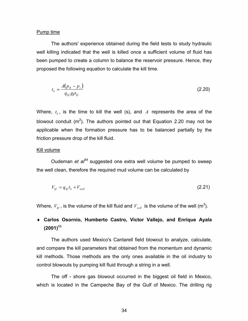
Pump time
The authors' experience obtained during the field tests to study hydraulic
well killing indicated that the well is killed once a sufficient volume of fluid has
been pumped to create a column to balance the reservoir pressure. Hence, they
proposed the following equation to calculate the kill time.
� �
kfkf
sRk gq
ppAt
�
�
� (2.20)
Where, kt , is the time to kill the well (s), and A represents the area of the
blowout conduit (m2). The authors pointed out that Equation 2.20 may not be
applicable when the formation pressure has to be balanced partially by the
friction pressure drop of the kill fluid. Kill volume
Oudeman et al54 suggested one extra well volume be pumped to sweep
the well clean, therefore the required mud volume can be calculated by
wellkkfkf VtqV �� (2.21)
Where, kfV , is the volume of the kill fluid and wellV is the volume of the well (m3). �� Carlos Osornio, Humberto Castro, Victor Vallejo, and Enrique Ayala
(2001)55
The authors used Mexico's Cantarell field blowout to analyze, calculate,
and compare the kill parameters that obtained from the momentum and dynamic
kill methods. Those methods are the only ones available in the oil industry to
control blowouts by pumping kill fluid through a string in a well.
The off - shore gas blowout occurred in the biggest oil field in Mexico,
which is located in the Campeche Bay of the Gulf of Mexico. The drilling rig

35
caught fire burning approximately 230 MMscfd. The gas flow rate was calculated
solving simultaneously the Forcheimer56 and Cullender and Smith21 equation.
Considering seawater as control fluid, the momentum kill study gave a kill flow
rate about three times greater than dynamic kill. The well was controlled with a
pump rate practically equal to that given by the dynamic kill method.
The authors conclude that the dynamic kill concept was a useful and
appropriate method to analyze and understand what happened during the
control, since the calculated and the real kill rate agreed very well. Another
conclusion from this study was that the assumption of a homogeneous flow at
high flow rates gave very good results. 2.3 Unsteady State Flow Models �� O. L. A. Santos and A. T. Bourgoyne (1989)57
Santos and Bourgoyne developed a simulator to predict loads imposed on
the diverter system and pressure peaks occurring during the well unloading
following an on - bottom shallow gas blowout. The study was conducted to
improve the design criteria and operating practices of the diverter system to
make their usage safer and more reliable during shallow blowouts. The
motivation was that the peak of pressure that occurs when the gas reaches the
surface has generated several failures of diverter equipment, leading to
blowouts. They built a mathematical model based on the simultaneous solution of
five equations: the continuity equation, the momentum balance equation, an
equation of state for the gas, a semi-empirical relationship between the gas and
liquid in - situ velocities, and a gas reservoir model.
The authors verified the model with data from experiments conducted at
the LSU Petroleum Engineering Research and Technology Transfer Laboratory
with a full scale well connected to a 6 - inch vent line. A variety of sensors were
placed to measure and record several important functions during the well

36
unloading process. Four drilling fluids with different properties were used during
the experiments.
Santos analyzed the diverter operations from some shallow gas drilling
environments utilizing the results given by the model and reached the following
conclusions. For most of the computer runs, the maximum pressure at the casing
shoe occurred when the gas reaches that point. Small diverter line diameters
resulted in high maximum wellhead pressure and high upward loads on the
upper portion of the well.
They also found out that the pressure peaks are caused by the fast
increase in velocity of the liquid flowing ahead of the two-phase mixture when the
gas approaches the surface. Hence, they recommend that the diverter system
components should be designed to withstand pressure as high as 1000 psi. �� Michael P. Starrett, A. Dan Hill, and Kamy Sepehrnoori (1990)43
Starrett et al developed a computer simulator of the flow and pressure
behavior in wellbores and diverters to predict performance during on - bottom
shallow gas blowouts. The authors considered four main zones: the reservoir, the
two-phase liquid/gas region in the wellbore, the liquid being displaced ahead of
the two-phase region, and the diverter piping.
The authors performed a simulation, and for the conditions simulated, they
found out that the pressure and velocity distributions were very responsive to
changes in bottom hole pressure, diverter diameter, and wellbore diameter, but
relatively insensitive to changes in initial circulation rate. Furthermore, they
conclude that the pressure and velocity behaviors depend strongly on the initial
differential between bottom hole pressure and reservoir pressure, and on the
wellbore and diverter diameters as determined by Santos et al57. �� Michael Wessel, and Brian Tarr (1991)28
Wessel and Tarr developed a method to control underground blowouts
based on the dynamic kill concept. The procedure proposes a set of equations to
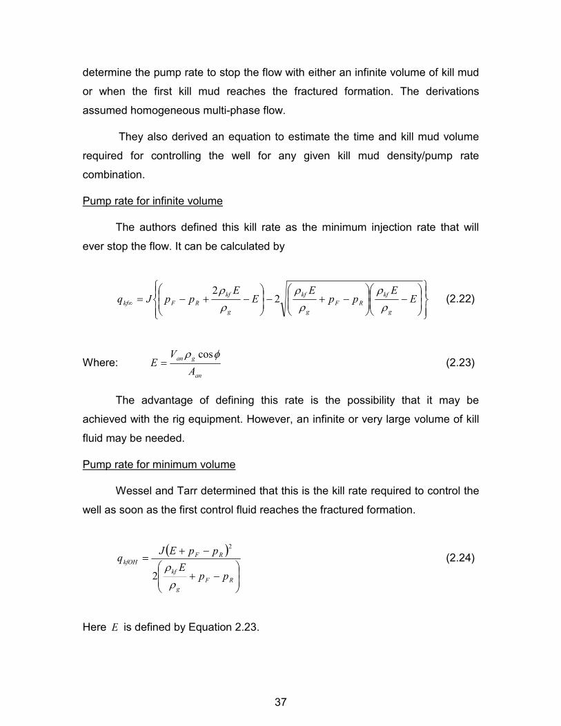
37
determine the pump rate to stop the flow with either an infinite volume of kill mud
or when the first kill mud reaches the fractured formation. The derivations
assumed homogeneous multi-phase flow.
They also derived an equation to estimate the time and kill mud volume
required for controlling the well for any given kill mud density/pump rate
combination. Pump rate for infinite volume
The authors defined this kill rate as the minimum injection rate that will
ever stop the flow. It can be calculated by
��
��
�
��
��
�
��
��
�
�
��
��
�
���
��
��
�
����
�E
Epp
EE
EppJq
g
kfRF
g
kf
g
kfRFkf
�
�
�
�
�
�2
2 (2.22)
Where: an
gan
AV
E�� cos
� (2.23)
The advantage of defining this rate is the possibility that it may be
achieved with the rig equipment. However, an infinite or very large volume of kill
fluid may be needed. Pump rate for minimum volume
Wessel and Tarr determined that this is the kill rate required to control the
well as soon as the first control fluid reaches the fractured formation.
� �
��
�
�
��
�
���
��
RFg
kf
RFkfOH
ppE
ppEJq
�
�2
2
(2.24)
Here E is defined by Equation 2.23.

38
Injection rates given by Equation 2.24 are usually high. Those high flow
rate requirements may not be achievable with available rig equipment, and
additional pumping units would be required. However, any combination between
Equations 2.22 and 2.24 would fulfill the requirements to kill the flow.
The authors also derived a method for determining the time and therefore
the kill mud volume to stop the underground flow and kill the well. It was based in
numerical integration of the equations that predict the rate of influx from the
formation and bottomhole pressure. They suggest that an estimate of the total kill
mud volume required is the volume pumped during the time required to stop
formation flow plus one annular volume. Once a kill pump rate and mud weight
are selected, these calculations can be made. The required mud volume should
be built before beginning the kill in order to execute the kill procedure without
interruptions.
Wessel and Tarr pointed out that the productivity index of a gas zone
flowing underground is approximately proportional to the product of the
formation's permeability and thickness. If this product is low, there is a good
probability of stopping the flow with the available rig equipment, but the
opportunity diminishes as formation productivity increases. Hence, by estimating
the formation permeability and thickness for a potential zone to be drilled, you
can determine whether an underground gas flow from the zone could be
controlled with the available rig equipment or whether additional pumping units or
relief well would be required. �� Adam T. Bourgoyne Jr., David Barnett, and Dan Eby (1996)58
Bourgoyne et al developed an advanced blowout control computer model.
It includes a steady state calculation option for quickly estimating the minimum
dynamic kill rate for a given kill fluid and well geometry. It also contains an
unsteady state flow option to estimate the volume of kill fluid needed and to
estimate a predicted pressure schedule during dynamic kill operations.
39
The authors used a modular approach to develop the model that provides
flexibility to simulate flow through the diverter system, surface blowouts and
underground blowouts that can be controlled with either an internal injection
string or one or more relief wells. They also included a flow section to allow the
analysis for flow through either a pipe or an annulus with alternative methods
commonly used for determining equivalent annular diameter. A flowing formation
model was coupled to wellbore system to compute the formation flow rate under
blowout conditions as well as formation fluid influx and bottomhole conditions
during the control.
The authors chose Excel 5.0 as the spreadsheet program to be used for
the application framework. They utilized subroutines to perform the more
complex calculations, which were written in Visual Basic. �� Fan Jun, Shi Tai-He, and Lian Zhang-Gui (1998)44
Fan Jun et al developed a dynamic kill model. It is capable of simulating
the complete blowout process giving results for the fluid distribution, flow rate,
fluid density, and pressure profile along the wellbore versus time. The model was
developed for gas blowouts and assumes that the drill string is placed at the
bottom of the hole during the complete blowout kill process.
The authors considered nine basic variables to describe the gas-liquid
flow system: gas and mud density, gas and mud velocity, gas volume fraction,
wellbore geometry, deviation angle, pressure and temperature. They adopted
homogeneous flow model in the wellbore, since the co-current flow system is of
rather high flow rate at the major stages in the kill process, which has been
proven accurate enough to characterize the flowing nature in the mist flow
regime.
Fan Jun et al included a gas reservoir model, which considers a non -
Darcy term due to the high flow velocity around the borehole. Then the wellbore
and reservoir mathematical models were linked, since any changes and

40
variations of the system performance in wellbore inevitably causes a response in
gas influx rate. �� O. L. A. Santos (2001)59
Santos developed a mathematical procedure to calculate the kill
parameters for a sea floor gas blowout. The procedure was based on the
concept of an on - bottom dynamic kill. The computer program also predicts the
time required to unload a deepwater well after its control has been lost, the gas
production rate, the total volume of gas produced during the blowout, and the
time and seawater injection rate required to dynamically kill the blowout.
The author coupled a wellbore model that predicts wellbore pressures to a
gas reservoir model that calculates gas flow rates entering the well during the
unloading part of the process and during the blowout itself. Santos established
the top end of the wellbore model at the sea floor as a boundary condition, which
is controlled by the hydrostatic pressure generated by the seawater. Hence, this
boundary condition value depends directly on water depth. He also considered in
his procedure both surface control by pumping kill fluid through an injection string
and control through a relief well.
Santos performed several simulation runs to analyze the effect of some
drilling variables, reservoir properties, and the effect of high backpressure
generated by seawater hydrostatic head on blowout flow rates and kill
parameters for a hypothetical deepwater scenario. Santos concluded that the
greater the well diameter, the greater both the gas flow and the required kill fluid
injection rate will be, since higher wellbore diameter provides smaller frictional
pressure losses. On the other hand, the increase in water depth results in lower
gas production rate due to seawater hydrostatic pressure at the wellhead.
The author also recommends that under no circumstances should an ultra
deepwater blowout be controlled using the surface diverter system. With flow to
the seafloor, the seawater backpressure restricts the blowout gas flow rate, and
that hydrostatic pressure will be lost if the diverter is employed since the riser will
41
be filled with gas after its unloading. Hence, if a gas kick is taken in an ultra
deep-water situation, the blowout preventers should be closed or the marine riser
disconnected. Simulation results showed that the riser can collapse at its bottom
due to the high differential pressure. He also pointed out that if the diverter
system is used, the very high gas flow rate can erode the equipment and the
presence of inflammable and explosive fluids on board can provoke disastrous
accidents.

42
CHAPTER 3
CURRENT ENGINEERING PROCEDURES FOR OFF - BOTTOM BLOWOUT CONTROL
Dynamic kill and momentum kill are currently the only two engineering
procedures that can be employed to analyze, design, and calculate the kill
parameters required to control an off - bottom blowout by pumping a fluid through
an internal injection string that conducts the kill mud into the wellbore. Both
methods have been used in field applications and have been reported to be
successful for controlling blowouts. The following section presents a study
performed to evaluate these concepts. 3.1 Dynamic Kill
Dynamic kill is a relatively new technique. It was developed by Mobil Oil
Corporation and was first reported by Blount and Soeiinah32. The method was
designed to control Indonesia's Arun field blowout. The well caught fire in June
1978, destroying the drilling rig and burning for 89 days at an approximate rate of
400 MMscfd. Due to the well's high deliverability and potential, it was expected to
be an extremely difficult well to kill. However, the engineering procedure was so
successful that the well was controlled one hour and 50 minutes after the kill
started.
3.1.1 Concept
The dynamic kill method to control blowouts uses fluid pumped from the
surface to a point downhole where it enters the blowout flow path to increase the
frictional pressure drop and the hydrostatic pressure over the length of the
blowout flow path. To obtain a successful kill, the summation of the frictional
pressure losses and the hydrostatic pressure due to fluid densities must be
greater than the formation pressure.

43
This concept can be better explained with Figure 3.1, which illustrates a
well and its pressure gradient. Section (a) shows the well with mud in static
conditions, with a hydrostatic pressure value at the bottom. In section (b), the
drilling mud is pumped through the injection string, and as shown by the shaded
area, the frictional pressure losses due to flow is used to increase the bottom
hole pressure. In a kill operation, that pressure increment will help to stop the
flow from the reservoir. However, it is important to avoid fracture of the open hole
formations, since if the formation breaks down part of the kill fluid will go into the
fracture, reducing the kill flow rate in the wellbore, and consequently the friction
losses. Thus the advantage of killing the well dynamically will be notably
reduced.
Figure 3.1 Effect of frictional pressure losses on bottom hole pressure
(Figure continued)
Hydrostatic pressure
Annular preventer
Fluid in static conditions
De p t h
Pressure
Static gradient
a) Static conditions

44
The main objective of the dynamic kill calculation technique is to
determine the minimum injection rate of available kill fluid necessary to stop
reservoir fluid flow into the wellbore (Kouba33). The method is designed to kill the
well by exceeding the natural flow capacity of the wellbore.
This technique is based on the steady state system analysis approach,
which consists of a study between the reservoir inflow performance and the
wellbore performance. System analysis, also known as NODAL analysis, has
been used in production wells and has received widespread acceptance in the oil
industry. Another successful application is in blowout control studies, since a well
under blowout conditions is very similar to a production well, with the difference
that the producing well is flowing under control and the reservoir fluids flow to the
production facilities rather than to the atmosphere.
Hydrostatic pressure
+ Frictional pressure
on the annulus
Frictional pressure drop
Drilling mud
Injection string
Annular preventer
Fluid in dynamic conditions
Shear stress at the pipe wall
De p t h
Pressure
Static gradient Dynamic gradient
fp�
b) Dynamic conditions

45
Figure 3.2 illustrates a blowout scenario. It can be seen that the reservoir
and the wellbore can act as a single hydraulic system and that the whole system
is affected by several factors such as reservoir pressure and properties,
formation fluid characteristics, and wellbore and drillstring geometry.
Figure 3.2 Reservoir and wellbore as a single hydraulic system
From Figure 3.2 it can be seen that the system has two important
components: the reservoir and the wellbore. The flow from the reservoir into the
well has been called "inflow performance," and a plot of producing rate versus
flowing bottomhole pressure is called an "inflow performance relationship"
(Beggs60). On the other hand, the "wellbore hydraulics performance" is given by
the flow behavior from the bottom of the well to the surface. Both inflow and
wellbore performance can be mathematically represented, and the simultaneous
solution of those analytical representations will give the relationship between the
IPR WHP Drill
string Wellbore
FBHP
Gas Flow Rate
Reservoir
FBHP
WBp�
Rp�
Rp�
WBp�

46
formation flow rate and the pressure drop for a specific spot. In the blowout
control area, that spot is typically selected as the bottom of the well. Hence when
the wellbore performance curve is above the inflow performance, the bottomhole
pressure is greater than the formation pressure and the reservoir no longer
produces.
3.1.2 Mathematical Model and Methodology
The inflow performance and wellbore hydraulics relationships will interact
to determine the conditions at which the dynamic kill will be achieved. Hence, the
following section will present a procedure applying this concept to determine the
required kill parameters for a gas blowout. The gas case was selected because
about 90% of all blowouts involve gas as reported in Chapter 2. The required kill
parameters include. �� Gas flow rate under blowout conditions
�� Pressure profile in the system under blowout conditions
�� Kill fluid density
�� Kill fluid injection rate
�� Pressure profile in the system at the beginning of the control and after
formation fluid influx stops
�� Surface pump pressure
�� Hydraulic horsepower
The required steps to design and compute the above kill parameters
utilizing the steady state system analysis approach are the following: 1. Compute the inflow performance relationship (IPR) for the reservoir and plot
it as function of flowing bottom hole pressure versus gas flow rate. Determination
of the inflow performance needs a connection between formation fluid flow rate
and the sand face pressure, and that relationship is given by a reservoir model
such as Equation 4.43. The IPR is built assuming different gas flow rates and
solving the equation for the bottomhole flowing pressure.

47
2. Compute the wellbore hydraulics performance curve and plot it as function of
flowing bottom hole pressure versus gas flow rate superimposed on the plot of
the IPR. Again determining the wellbore performance requires a relationship
between formation fluid flow rate and the bottom hole pressure, which is given by
the Cullender and Smith model, Equation 4.44. The wellbore hydraulic
performance is completed assuming different gas flow rates and solving the
equation at the sand face. Figure 3.3 displays a typical behavior of the system
analysis. The IPR curve shows the performance of the reservoir, and the WHP
curve represents the performance of the wellbore when flowing only gas, in other
words the pressures required to move the resulting rates of gas through the
wellbore system to the atmosphere. 3. Determine the gas flow rate under blowout conditions, which is given by the
intersection of the inflow performance curve "IPR" and the wellbore hydraulics
performance curve "WHP" on Figure 3.3. This situation indicates that the well
has been completely unloaded of all liquid, except any that is flowing from the
formation, and a free flowing equilibrium condition has been reached.
Figure 3.3 Reservoir inflow performance and wellbore hydraulic performance at blowout conditions
FB H P
Gas Flow Rate
IPR
WHP
Simultaneous solution is given at the intersection
Gas flow rate
Bottom hole pressure

48
4. Plot the pressure profile in the well under blowout conditions utilizing the gas
flow rate obtained in the previous step and Equation 4.44. This equation is solved
for small depth increments in the wellbore. 5. Compute the wellbore hydraulics performance curve for each of various kill
fluid injection rates with one selected kill fluid density in combination with a range
of gas flow rates up to blowout flow rate, then plot them on the graph
accomplished in step 2. These curves are calculated taking into account
pressure changes due to elevation, friction, and acceleration of the mixture. They
are obtained utilizing Equation 4.29 and the respective fluid property correlations
given in Chapter 4. Figure 3.4 illustrates the wellbore hydraulics performance
curves for different injection rates. Analyzing one of these lines, it can be seen
that as the gas flow rate increases from zero, the bottom hole pressure typically
decreases due to reduction in hydrostatic pressure. This portion of the curve
shown as a dashed line is referred to as being hydrostatically dominated. On the
other hand, further increases in the gas flow rate eventually increase the bottom
hole pressure due to increasing frictional pressure losses. Consequently, this
segment of the curve shown as a solid line is known as friction dominated. 6. Select the kill injection rate from the plot as the line of constant injection rate,
which is just above or tangent to the inflow performance relationship curve.
Therefore, injection rate #3 on Figure 3.4 is the lowest rate that will achieve a kill.
At that kill fluid rate, a stable gas lift flow condition would not be possible, and the
well would be killed. On the other hand, if the wellbore hydraulics performance
intersects the reservoir performance curve, as for injection rate #2, then a stable
flow condition would result. That is, the reservoir would continue to produce at
the rate corresponding to the point of intersection, and the well would not be
killed.

49
Figure 3.4 Wellbore hydraulics performance for various kill fluid injection rates
7. If the selected kill injection rate is too high to handle with the available
pumping equipment, repeat steps 5 and 6 with a higher kill density. Otherwise,
proceed with step 8. 8. Plot the pressure profile in the system as a function of depth for the selected
kill injection rate and density. This will give a good approximation of the pressure
conditions in the wellbore just after the formation fluid influx stops. Hence those
pressures can be compared with the burst ratings of the wellbore tubulars and
the fracture pressure in the open hole interval. 9. Estimate the frictional pressure losses and the hydrostatic pressure in the
injection string utilizing Equations 4.62 and 4.63 respectively as well as the
selected kill flow rate and kill fluid density. 10. Calculate the surface injection pressure employing the frictional pressure
losses and the hydrostatic pressure previously calculated and Equation 4.61
Gas Flow Rate
FB H P
Injection Rate # 1
only gas flowing
Injection Rate # 2
Injection Rate # 3
1 # 2 # 3 # IRIRIR ��Hydrostatic dominated Friction dominated
50
11. Determine the hydraulic horsepower requirement using the surface injection
pressure from the previous step.
This procedure is represented by the flow chart in Figure 3.5, which shows
the algorithm utilized to estimate the kill parameters applying this theory.
A real blowout control calculation presented in the next section will be
used to explain this procedure in detail.
Some blowouts necessitate very high pump pressure and horsepower to
be controlled, which is not always possible with the equipment available on the
site. Nevertheless, those parameters can be reduced by use of special drag
reducing fluid additives. If a friction reducer is present in the kill fluid, it should be
taken into account to calculate the frictional losses in the system. But if the pump
pressure and horsepower cannot be reduced to acceptable limits, either
additional pumping units or a relief well will be needed.
3.1.3 Computer Program
One of the aims of this research was to investigate how the current
blowout control methods perform at off - bottom conditions, as well as describe
their deficiencies and limitations. In order to achieve this goal, a computer
program is desirable to perform calculations to analyze several blowout control
scenarios.
Therefore, a dynamic kill computer program following the previous
procedure was created to accomplish the analysis. It is important to point out that
the program was based on the conventional dynamic method, which assumes
that only formation fluid is present below the injection point. This consideration is
contemplated in nearly all current published models, and most consider just the
hydrostatic head of the fluid. In this program all the components of the pressure
gradient equation are considered (hydrostatic head, friction losses, and
acceleration).

51
Collect the blowout data
Determine the reservoir and fluid properties
Compute the IPR
Compute the WHP when only gas is flowing
Determine the gas flow rate and FBHP
Plot the flowing pressure profile
Select a kill flow rate and density
Recalculate the WHP for the selected kill rate and density
Is the WHP always
above the IPR?
Required Kill flow rate and density are obtained
Does the pumping
system have capacity to pump the
selected rate
Plot pressure profile utilizing only kill rate and density
Does the casing or the open hole support the maximum
pressure imposed for those flow conditions
Increase either kill flow rate or kill density
Modify kill flow rate, kill density, or increase string depth. Otherwise, consider another control technique (capping, relief well)
No
Yes
No
Yes
Yes
Increase string depth or obtain another pumping system. Otherwise consider another control technique (capping, relief well)
No
B
A
A
Figure 3.5 Algorithm to estimate the dynamic kill parameters (Figure continued)

52
Determine the frictional pressure losses in the injection string
Calculate the surface injection pressure
Determine the hydraulic horsepower
Does the pumping
system meet the required hydraulic
horsepower
Solution is reached and the kill parameters are predicted
Once the computer program was finished, it was compared to previously
published examples to evaluate its performance. The calibration was carried out
using field data and results from other models published in the literature. 32, 33, 53
Table 3.1 Blowout data from Mobil Oil Indonesia's Arun field well No. C-II-232
Input Data
Reservoir pressure (psia) 7,100
Reservoir temperature (°F) 230
Gas specific gravity 0.6
Casing ID (in) 8.535
Drillpipe OD (in) 5.00
Drillpipe ID (in) 4.275
Pipe roughness (in) 0.0018
Measured depth (ft) 10,210
True vertical depth (ft) 9,650
B
Yes
Modify string depth or obtain another pumping system. Otherwise consider another control technique (capping, relief well)
No
A
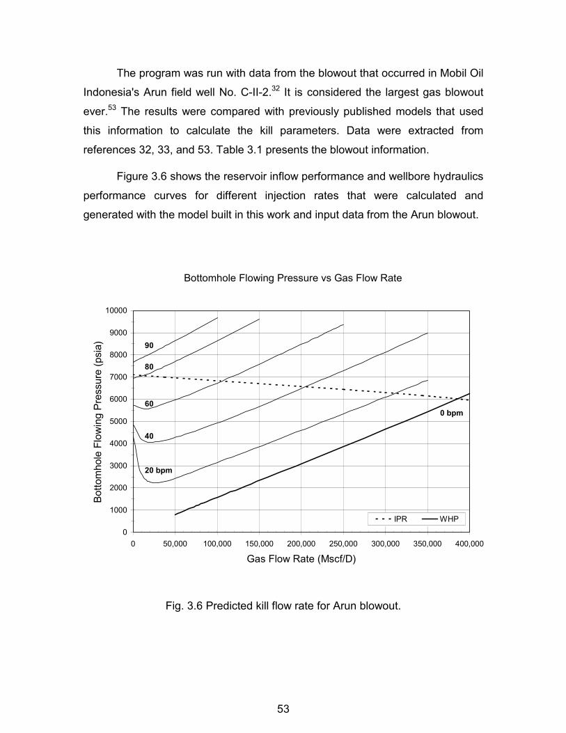
53
The program was run with data from the blowout that occurred in Mobil Oil
Indonesia's Arun field well No. C-II-2.32 It is considered the largest gas blowout
ever.53 The results were compared with previously published models that used
this information to calculate the kill parameters. Data were extracted from
references 32, 33, and 53. Table 3.1 presents the blowout information.
Figure 3.6 shows the reservoir inflow performance and wellbore hydraulics
performance curves for different injection rates that were calculated and
generated with the model built in this work and input data from the Arun blowout.
Fig. 3.6 Predicted kill flow rate for Arun blowout.
Bottomhole Flowing Pressure vs Gas Flow Rate
0
1000
2000
3000
4000
5000
6000
7000
8000
9000
10000
0 50,000 100,000 150,000 200,000 250,000 300,000 350,000 400,000
Gas Flow Rate (Mscf/D)
Botto
mho
le F
low
ing
Pres
sure
(psi
a)
IPR WHP
90
80
60
40
20 bpm
0 bpm

54
Analysis of the results of the Arun blowout calculation, see Figure 3.6,
showed the following. The inflow performance curve "IPR" shows the
performance of the reservoir. The "0 bpm" curve represents the wellbore
performance of the system when only gas is flowing. The intersection of the
"IPR" curve and "0 bpm" curve corresponds to the well condition after all of the
liquid has been unloaded from the wellbore and free flowing equilibrium condition
has been reached. According to the calculations given by the program, the Arun
field's well No. C-II-2 was producing at an approximate rate of 380 MMscfd
during the blowout, with a bottom hole pressure around 6,000 psi.
Figure 3.6 also shows an injection of water at a rate of 20 bpm down the
drillpipe would result in a stable flow condition. That is, the reservoir would
continue to produce at a gas flow rate of about 310 MMscfd and a bottom hole
pressure around 6,400 psi. A stable flow condition would also result for an
injection rate of 40 bpm with a producing rate and bottom hole pressure of 205
MMscfd and 6,600 psi respectively. As can be seen from this system analysis
approach, it is expected that the well passes through a series of flowing
conditions during the control due to kill fluid entering the annulus.
In achieving a dynamic kill of the Arun blowout, the calculations indicate
that a water injection rate of approximately 83 bpm would give a bottom hole
pressure of 7,100 psi, which would be enough to create sufficient backpressure
at the formation face to prevent further gas flow from the reservoir.
The solutions for the Arun blowout given by others' dynamic kill models
are presented in Table 3.2. It can be seen in that the dynamic kill computer
program developed in this work has excellent agreement with other models. It
may therefore be used with confidence to perform the sensitivity analysis for
different blowout scenarios and detect the reach and limitations of the dynamic
kill method during blowout control operations with the injection string at off -
bottom conditions.
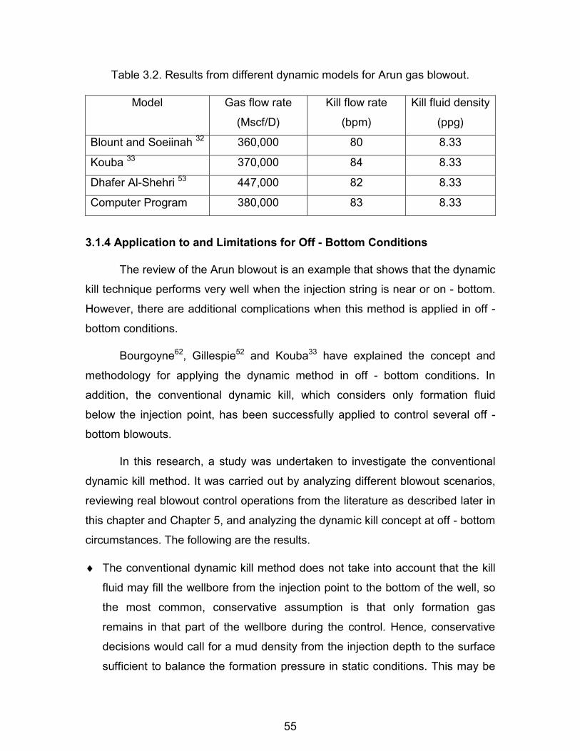
55
Table 3.2. Results from different dynamic models for Arun gas blowout.
Model Gas flow rate
(Mscf/D)
Kill flow rate
(bpm)
Kill fluid density
(ppg)
Blount and Soeiinah 32 360,000 80 8.33
Kouba 33 370,000 84 8.33
Dhafer Al-Shehri 53 447,000 82 8.33
Computer Program 380,000 83 8.33
3.1.4 Application to and Limitations for Off - Bottom Conditions
The review of the Arun blowout is an example that shows that the dynamic
kill technique performs very well when the injection string is near or on - bottom.
However, there are additional complications when this method is applied in off -
bottom conditions.
Bourgoyne62, Gillespie52 and Kouba33 have explained the concept and
methodology for applying the dynamic method in off - bottom conditions. In
addition, the conventional dynamic kill, which considers only formation fluid
below the injection point, has been successfully applied to control several off -
bottom blowouts.
In this research, a study was undertaken to investigate the conventional
dynamic kill method. It was carried out by analyzing different blowout scenarios,
reviewing real blowout control operations from the literature as described later in
this chapter and Chapter 5, and analyzing the dynamic kill concept at off - bottom
circumstances. The following are the results. �� The conventional dynamic kill method does not take into account that the kill
fluid may fill the wellbore from the injection point to the bottom of the well, so
the most common, conservative assumption is that only formation gas
remains in that part of the wellbore during the control. Hence, conservative
decisions would call for a mud density from the injection depth to the surface
sufficient to balance the formation pressure in static conditions. This may be

56
impossible to achieve when the formation pressure is high and the length
between the surface and the injection depth is short, see Figure 3.7. Due to
this fact, the opportunity to develop an in - well control would be discarded,
and another more expensive and time consuming blowout control
methodology such as snubbing in or relief well would be considered.
Figure 3.7 Effect of short injection string on dynamic kill
�� The dynamic kill method is not guaranteed to displace, or remove completely,
the formation fluid from the injection point to the bottom of the well. Its design
considers stopping the flow with bottomhole pressure just reaching the
formation pressure. Therefore, the pressure is inadequate to force the kill fluid
to flow from the injection point down into the producing zone. If the injection
string depth is distant from the bottom in an authentic off - bottom scenario, a
considerable amount of gas may remain in the section below the injection
point. If the circulation rate is reduced or stopped, it may start to migrate,
Kill fluid
Kick formation
Formation gas
Injection string
Injection string length
� �L
Reservoir pressure
� �Rp
Lp kfR ��� �052.0
�� kfLif �

57
expanding, and forcing some drilling fluid out of the well. Consequently, the
average density will be reduced in the system, and the well may begin to
unload again. Figure 3.8 illustrates this event.
Figure 3.8. The well may unload if a considerable amount of gas
remains in the wellbore
�� The dynamic kill is based on the steady state system analysis approach51,
and it was earlier shown that the system analysis is a relationship between
the reservoir inflow performance and the wellbore hydraulic performance. For
blowout control applications, performance is plotted on a bottom hole
pressure versus gas flow rate graph such as Figure 3.2. If an off - bottom
condition is presented this approach cannot be precisely employed to analyze
and compute the kill parameters because of the uncertainty about the real
conditions and mixture properties below the injection depth. Consequently,
Producing zone
Formation gas
Kill mud
Expanded gas

58
the pressure gradient cannot be accurately known between the injection
depth and the formation depth. As a result, the wellbore hydraulic
performance curves cannot be accurately determined. This scenario is
schematically illustrated in Figure 3.9.
Figure 3.9 Effect of utilizing system analysis approach in off -bottom scenarios
�� Another disadvantage of the dynamic kill is that its design sometimes uses a
fluid to control the well dynamically that is less dense than the fluid needed for
a hydrostatic kill. The fluid would then have to be changed for a heavier one
to maintain control in static conditions. Consequently, additional operations
have to be planned and implemented properly to get a final control. This
increases the complexity and risk of mistakes in conducting the kill.
Gas bearing zone
Kill fluid
Injected kill fluid
Injection string
Formation gas
Unknown mixture properties:
Unknown pressure gradient:
Unknown bottom conditions:
Erroneous wellbore hydraulic performance curve
� �mixturev , , ��
� �totalp�
influxGasFBHP ,
Wrong kill parameters determination

59
�� The current off - bottom dynamic kill methods described by Gillespie52 and in
more detail by Kouba33 provide means for predicting wellbore hydraulic
performance below the injection point. However they do not present a
procedure for knowing when the lower wellbore section below the injection
depth is completely filled with kill mud. The volume that must be pumped to
make sure that the lower zone is completely full and the kill operation
completed is unknown. 3.2 Momentum Kill
The momentum kill is a procedure based on fluid dynamics and was first
reported in 19776 as a method that can be utilized to control off - bottom blowouts
without tripping in to the bottom of the well. Grace6 and Watson7 have described
the concept and mathematical model of this procedure as an alternative solution
for off - bottom blowouts. Grace 8,9 has also described successful control of
blowouts by applying this technique. 3.2.1 Concept
The momentum kill is based on the concept that when two fluids traveling
in opposite directions collide, the one with greater momentum controls the
direction of flow for both. Therefore, in the blowout control operation proposed by
these authors, the formation fluid and the kill fluid collide at the injection string
depth. Conceptually, the momentum of the control fluid must be greater than the
momentum of the formation fluid to stop the blowout fluid and force it back into
the formation and to bring the well under control. This concept is schematically
illustrated in Figure 3.10
This procedure uses the kill fluid velocity and density to generate a greater
momentum than that the formation fluid flow. Therefore, either high pump rates
or kill densities are expected when this technique is utilized to design a blowout
control. Consequently, a detailed analysis should be performed on the tubulars in
the well and on the open hole in order to guarantee that they can contain the
pressures during the control operation36.

60
Figure 3.10 Kill and formation fluid collision at injection string depth
Applying this concept, the kill density employed to control the well should
generate enough hydrostatic pressure to control the formation pressure in static
conditions. Once the pump stops, the momentum of the kill fluid becomes
nothing and the only way to keep the well under control is by utilizing the
hydrostatic pressure of the drilling mud. 3.2.2 Mathematical Model and Methodology
The mathematical model of momentum kill is based on the Newton's
Second Law of Motion16, which states that the net force acting on a system is
equal to the rate of change of momentum of that system. Only forces acting at
the boundaries of a prescribed space are concerned: any force within the space
is involved only as one half of an "action - and - reaction" pair and so does not
Formation fluid
Kill fluid
Reservoir
Kill fluid
Injection string
Collision depth
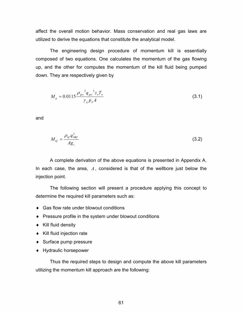
61
affect the overall motion behavior. Mass conservation and real gas laws are
utilized to derive the equations that constitute the analytical model.
The engineering design procedure of momentum kill is essentially
composed of two equations. One calculates the momentum of the gas flowing
up, and the other for computes the momentum of the kill fluid being pumped
down. They are respectively given by
ApTzq
Mng
nngscgscg
�
�22
0115.0� (3.1)
and
c
Mkfkfkf Ag
qM
2�
� (3.2)
A complete derivation of the above equations is presented in Appendix A.
In each case, the area, A , considered is that of the wellbore just below the
injection point.
The following section will present a procedure applying this concept to
determine the required kill parameters such as: �� Gas flow rate under blowout conditions
�� Pressure profile in the system under blowout conditions
�� Kill fluid density
�� Kill fluid injection rate
�� Surface pump pressure
�� Hydraulic horsepower
Thus the required steps to design and compute the above kill parameters
utilizing the momentum kill approach are the following:

62
1. Determine the gas flow rate and pressure profile in the system under blowout
conditions, which is given by the procedure explained in the dynamic kill
section 3.1.2 (steps 1 through 4). 2. Calculate the profile of the gas deviation factor in the system utilizing the
Equation 4.24. 3. Compute the profile of the gas density in the system employing Equation
4.22. 4. Estimate the profile of the momentum of the gas with equation 3.1, and plot it
versus depth. 5. Calculate the momentum of the kill fluid employing equation 3.2, for various
kill fluid injection rates and kill densities that can be handled with the available
pumping units. The selected densities should generate enough hydrostatic
pressure to control the formation pressure in static conditions, but those
hydrostatic columns should not reach the fracture pressure. 6. Superimpose the momentum of the kill fluid calculated in step 5 on the plot of
step 4. Select the kill rate and density combination that matches or exceeds
the momentum of the gas at the injection string depth. 7. If the selected kill injection rate is too high to handle with the available
pumping equipment, repeat step 5 with a higher kill density.
This procedure is represented by the flow chart in Figure 3.11, which
shows the algorithm utilized to estimate the kill parameters applying this theory. 3.2.3 Computer Program
A computer program was developed utilizing the momentum kill concept
with the objective of developing a sensitivity analysis in order to know how this
method performs under different blowout scenarios by changing parameters such
as formation properties, reservoir fluid properties, formation fluid flow rate,
wellbore and tubulars geometries, and injection depth.

63
Collect the blowout data
Determine the reservoir and fluid properties
Compute the IPR
Compute the WHP when only gas is flowing
Determine the gas flow rate and FBHP, and plot pressure profile
Estimate the profile of the gas deviation factor
Compute the profile of the gas density
Determine the momentum of the gas and plot it versus depth
Select a kill flow rate and density
Calculate the momentum of the kill fluid and plot it on previous graph
Is the momentum of the kill fluid
greater than the momentum of the formation fluid?
Required kill flow rate and density are obtained
Does the pumping
system have capacity to pump the
selected rate
Solution is reached and the kill parameters are predicted
Figure 3.11 Algorithm to estimate the momentum kill parameters
The momentum kill program was based on the mathematical model and
procedure previously presented. Once the computer program was finished, it was
Increase either kill flow rate or kill density
No
Yes
Increases string depth or obtain another pumping system. Otherwise consider another control technique (dynamic kill capping, relief well)
No
Yes

64
validated, using field data and results published in the literature.8 Table 3.3
shows that the results from the momentum kill computer program developed in
this work match with the published results8. Therefore, it can be used to analyze
additional blowout scenarios and to formulate conclusions about this method.
Table 3.3 Comparison of momentum kill results. Momentum of the gas Momentum of the kill fluid
12 ppg 20 ppg
Published Results8 6.8 lbf 8.9 lbf 14.8lbf
Program Results 6.8 lbf 8.9 lbf 14.8lbf
3.2.4 Momentum Kill Analysis
An analysis was performed on momentum kill in order to determine its
performance. The study concentrated mainly on the following elements.
�� Careful derivation of momentum equations to give a logical analysis of the
concept. �� An analytical study applying a pressure profile analysis and the critical
velocity concept to investigate the flow direction after the collision between
the kill fluid and the formation fluid.
�� An analysis of the two published blowouts in the literature that used this
concept to regain the control of the well in order to understand what
actually controlled those wells. And calculate and compare the kill
parameters for different blowout scenarios utilizing both the momentum
and dynamic concept.
3.2.4.1 Analytical Study
This part of the work presents an analytical study performed on the
momentum kill concept. The study focused on two elements: an analysis of the
derivation of the momentum equations used in the engineering design procedure

65
and an analysis of the flow direction after the collision between the formation fluid
and kill fluid.
The engineering design procedure of the momentum kill concept is
described as being based on Newton's Second Law of Motion16, which is
mathematically represented by
� �dt
MomentumddtdvmmaF
External���� (3.3)
Applying the control volume formulation to the linear momentum of the system17:
� ���
�
����
cvcs
dVvt
dAvvdt
Momentumd�� (3.4)
Combining Equation 3.3 and 3.4:
����
����
cvcsExternal dVv
tdAvvF �� (3.5)
Where v represents the fluid velocity, � the fluid density, A the flow area and V
is the volume in the control volume. Equation 3.5 is called the control volume
formulation of Newton's Second Law, also known as the linear momentum
equation. It states that the summation of all external forces (body, normal, and
frictional) on a system is equal to the rate of change of momentum of that
system.
In a blowout scenario a reasonable consideration is that steady state has
been reached after the well has been completely unloaded of all the mud and
only formation fluid is flowing through the well. Thus, Eq. 3.5 becomes:
�� ��
csExternal dAvvF � (3.6)

66
Considering intervals with constant area the above equation becomes:
vAvFExternal ��� (3.7)
Replacing the velocities by Aqv /� and introducing the constant of
proportionality in Equation 3.7:
Agq
FFc
Mkfkf
changeMomentumExternal
2�
��� (3.8)
Equation 3.8 is the relationship to compute the momentum force of an
incompressible fluid, in this case kill mud. The equation to calculate the
momentum force of a compressible fluid such as formation gas, is obtained if the
principle of mass conservation and real gas law is applied to Equation 3.8, see
Appendix A for the derivation, this is given by
cnag
gscgsc
changeMomentumExternal AgpM
zRTqFF
�
�22
��� (3.9)
The procedure that the momentum kill method utilizes to calculate the kill
rate and density combination is to require the momentum of the kill fluid (Eq. 3.8)
to be equal to greater than the momentum of the formation gas (Eq. 3.9).
cnag
nngscgsc
c
Mkfkf
AgpMRTzq
Agq
�
��222
�
Then, for a given kill density, the above equality is solved for the kill flow rate as
follows:

67
21
22
��
�
�
��
�
��
��
��
�
�
kf
c
cnag
nngscgscMkf
AgAgpMRTzq
q��
� (3.10)
However, the force term on the left hand side (� ExternalF ) of Eq. 3.8 and
3.9, that is neglected by the published momentum design procedure, is the sum
of all forces acting in the system
� ��� ��� BTPExternal FFFF (3.11)
Where PF is the normal force, and it is due to the pressure into the system. It is
given by
��
csP dApF
Where: �p Pressure
�A Flow area
The tangential force ( TF ) is due to the viscous shearing stress of the fluid
over the wellbore and pipe wall. It is mathematically represented by
� ��
csT dF �
Where: �� Shear stress
�� Contact area
And finally BF is the body force, and it is due to the gravity force, which
acts in the direction of the gravitational field. It is given by
��
cvB dVgF �

68
Where: �g Acceleration of gravity
�� Fluid density
�V Volume of fluid
Hence ���� �����
cvcscscs
dVgddApdAvv ���
The equality of the rate of change of momentum and the external forces
(Newton's Second Law of Motion) gives the conservation of momentum
equation34 for flow in a linear system. It is presented in pressure instead of force
and for upward flow direction and pressure drop defined as positive when
upstream pressure is greater than downstream pressure.
gAd
dLdpv
dLd
��
�� ���)( 2
The pressure gradient equation34 is obtained combining both the
conservation of momentum and conservation of mass equations (see Appendix
B), and is given by:
elevationfrictiononaccelerati pppp �������
Therefore, the forces given by the Newton's Second Law of Motion become:
elevationfrictiononaccelerati
bodytangentialnormalchangemomentum
pppp
FFFF
�������
���
The fundamental concept of well control states that the bottomhole
pressure must be greater than or at least equal to the formation pressure to stop
the formation flow.

69
formationbh pp �� or for a surface blowout formationsurf ppp ���
It can be seen that the momentum kill design concept presumes to reach
the formation pressure and stop the flow by considering only the acceleration
component of Newton’s second law of motion. Both the friction and elevation
terms are neglected and it is well known that these components play a very
important role in these scenarios since they almost always have the largest
magnitude in a blowout control. Examples of the relative magnitudes of
pressures, which cause these forces, are given in section 3.2.4.2. Therefore, if
the procedure considers Newton's Second Law of Motion as its basic equation,
the external forces must be considered.
Another analysis of this procedure was an investigation of the flow
direction after the collision between the formation fluid and kill fluid. This
investigation was based on the analytical work performed by Turner et al61,
Gillespie et al52, and Kouba et al33. They considered that liquid droplets entrained
in a gas stream will be lifted out if the gas velocity is greater than the critical gas
velocity. This concept was also, experimentally proved by Bourgoyne et al62 and
Flores et al63.
Therefore, this theory states that if the gas velocity at the injection string
depth in the blowout well is greater than the critical gas velocity, the gas stream
will lift out the kill fluid after the control operation begins. And as a result, the
possibility of stopping the flow due to the collision between the formation and kill
fluid and force the gas back into the formation will be minimal. The gas velocity,
when only formation gas is flowing through the well, depends on reservoir and
reservoir fluid properties as well as wellbore geometry. But just as soon as the
control operations start, the conditions at the well (pressure profile, gas influx,
fluid properties, etc) begin to change because of kill mud presence. As a
consequence, the speed of the gas decreases to such level that the critical gas
velocity may be reached and kill fluid may begin to fall below of the injection
point.

70
However the momentum method does not consider that the conditions in
the system are continuously changing, since its design calls for stopping the
blowing fluid at the instant of collision. But it is expected that the formation gas is
at its maximum velocity just before the impact or before the kill fluid begins to
flow from the injection depth to the surface. This is because the bottom hole
pressure is at a minimum value hence the gas flow rate reaches its maximum
value. Thus the key factor to consider whether the kill fluid may be ejected by the
gas stream is determined by critical gas velocity, which is the minimum velocity
that will lift all liquid entering the flow path. It is a function of the size, shape, and
density of the mud particle and density and viscosity of the gas medium. The
critical gas velocity is estimated as follows.
Gillespie et al52 presented a procedure to calculate the critical gas velocity.
Their method considers two factors: the largest diameter of droplet likely to exist
in the gas stream and a conservative value for the drag coefficient of the droplet.
They used three approaches to estimate the maximum likely droplet size. In this
analysis only two of them will be presented, those that presented the maximum
and minimum critical velocity (in other words, the extreme cases). One of the
approaches was elaborated by Karabelas; it is given by
6.0295max4
���
����
���
�
� cci
i
vd
ddd (3.12)
The other one was developed by Sleicher, it is calculated by
��
�
�
��
�
�
���
�
� �
7.0
2max 7.0138�
�
�
�
�
�
c
d
c
c
cc gv
vg
vd (3.13)
When the relative settling velocity of the largest droplet is just equal to or
greater than the average gas velocity, the fluid will be able to fall below of the
injection point. Otherwise, the gas will sweep all droplets out of the well.

71
The critical gas velocity or the settling velocity of a drop is obtained by
� �
dc
cdcrit K
gdv
�
��
34 max �
� (3.14)
In Equation 3.14, dK represents the drag coefficient, which is function of the
Reynolds number based on the slip velocity.
c
critcvdN
�
�maxRe � (3.15)
The equation proposed by Gillespie to compute the drag coefficient is the
following:
��
���
���� 5.0424
468.0ReRe NN
FKd (3.16)
Equation 3.16 gives a conservative estimation of the drag coefficient in
quiescent fluid that neglects the sudden drop in value of dK associated with
reaching the critical Reynolds number. On the other hand, F is the factor to
account for effect of turbulence on dK . They considered the analysis developed
by Lopez and Dukler, which gave a value of 4�F . This value accounts for
some gas turbulence intensity levels. The methodology to calculate the critical
gas velocity using the above method is the following: 1. The maximum likely droplet size ( maxd ) is calculated using the Equations 3.12
and 3.13.
2. A value of the drag coefficient ( dK ) is assumed. A good initial value may be
0.44

72
3. Using the guess value of the drag coefficient, the critical gas velocity is
calculated with Equation 3.14.
4. The Reynolds number given by Equation 3.15 is computed with the critical
gas velocity obtained in step 3.
5. The drag coefficient given by Equation 3.16 is estimated utilizing the
Reynolds's number previously calculated.
6. Again, the critical gas velocity is calculated using the drag coefficient obtained
in the previous step.
7. The critical gas velocities from step 3 and 6 are compared; if they are close
enough, the process finishes. Otherwise, repeat the procedure from step 3 to
7 until the critical gas velocities are sufficiently close.
Another procedure to calculate the critical gas velocity is given by Kouba
et al 33. They used Taitel, Barnea, and Dukler's mechanistic model. The transition
boundary between annular and non-annular flow was developed from a force
balance on a droplet of liquid in gas stream. The transition is marked by the
minimum gas velocity required to suspend a liquid droplet.
� �4/1
2593.1���
�
���
� ��
g
cdcritv
�
��� (3.17)
The above approach has been used successfully by Coleman to
determine when low-pressure gas would begin liquid unloading. Equation 3.17 was rewritten in terms of standard volumetric flow rate as follows:
� �4/1
287.4���
�
���
� ��
g
cd
pgsc Tz
Apq�
��� (3.18)
When the formation fluid flow rate is lower than the one given by Equation
3.18, the injection liquid will begin to fall below of the injection point.

73
The critical velocity concept was applied to the condition in a blowout
described by Grace8. The results are presented in Figure 3.12.
Figure 3.12 Critical gas velocity versus in-situ gas velocity for an actual blowout 8
Figure 3.12 displays the estimated critical gas velocity profile utilizing
three different approaches. Those velocity profiles were obtained from about
2,300 ft to the beginning of the injection string (nine drill collars). It can be seen
that Karabelas' approach gives a critical velocity of 3 ft/s, which means that the
kill mud might fall below of the injection point when the in-situ gas velocity has
decreased about to 3 ft/s. On the other hand, Kouba's method yields about 9
ft/sec. However the estimated in - situ gas velocity at 2300 ft before starting the
control operation is greater than 21 ft/sec and greater than 200 ft/sec when the
gas reaches the drill collars. Hence, following the critical velocity theory, this
analysis indicates that the gas stream at the injection point would eject the kill
In-situ gas velocity
270
690
1,110
1,530
1,950
2,370
0 2 4 6 8 102 4 6 8 10
Critical Gas Velocity (ft/sec) In-situ Gas Velocity (ft/sec)
20 90 160 230
SleicherKarabelas Kouba

74
fluid. Consequently, it seems unlikely that the kill fluid would instantaneously stop
the gas flow and move downward as envisioned in the momentum kill concept. 3.2.4.2 Analysis of Actual Blowouts Controlled by Applying the Momentum
Method
This section describes an analysis of actual blowouts that were controlled
by applying the momentum or dynamic kill concept. It was performed with the
goal of understanding the actual mechanics of each kill. The three blowouts were
originally described in references 8, 9, and 55.
One blowout presented by Grace8 occurred in Carbon County, Wyoming.
It occurred during a washover and backoff operation, with three 6" drill collars
above the rotary table and six 7" drill collars below the rotary table. The blowout
scenario is presented in Figure 3.13.
Figure 3.13 Blowout conditions given by Grace8
TOF at 2,350 ft TD 3,000 ft
Gas + Water
9 5/8” 1,500 ft
13 3/8” 400 ft
End of string 180 ft
Kill line 2” p = 820 psig
Six 7” drill collars Three 6” drill collars
75
In the blowout well, around 30 MMscfd of gas plus water were flowing
through the drill collars to the atmosphere. The annular preventer was closed,
and the only access to the well was through the kill line. The procedure selected
to design the blowout control and calculate the kill parameters was the
momentum kill. The momentum force of the gas, gM in Equation 3.1, was
calculated to be 6.8 lbf, but it was thought that the water increased the total
momentum to about 14 lbf. During the control, two kill attempts were performed.
First, 12-ppg fluid and a rate of 12 bpm were unsuccessfully employed. These
conditions gave a momentum force of the liquid, kfM in Equation 3.2 of 8.9 lbf.
The second kill attempt utilized a 20 ppg kill mud and a rate of 12 to 13 bpm was
selected. These kill conditions gave a momentum force of 14.84 lbf. Following
the concept of this method, this would be more than the minimum force required
to change the gas velocity to zero and then displace if downward through the
wellbore if gravitational and drag forces are ignored. The well was successfully
controlled, using the selected kill parameters, at a pumping pressure of 1300 psi.
The dynamic kill computer program for this research study was utilized to
analyze this kill from the perspective of the dynamic kill concept. The program
uses the conventional dynamic method, which considers that only formation fluid
is below the injection point. The program computes the pressure gradient in both
upper and lower sections considering friction, elevation, and acceleration terms.
Due to the fact that the amount of water flowing in the system was
unknown, the calculation considers only gas as blowout fluid. However, this
consideration gives lower bottom hole flowing pressures during the dynamic
control process than the actual ones, since water increases both the friction and
elevation components.
Figure 3.14 shows the wellbore hydraulics performances as solid lines
given by the dynamic kill calculation and the kill parameters used to control this
well; the dashed curve represents the wellbore hydraulic conditions when only
formation fluid is flowing. The reservoir inflow performance was not calculated

76
because the reservoir pressure and properties were not reported. However, two
reasonable bottomhole pressure conditions were adopted. One bottomhole
pressure value was calculated using the gas flow rate of 30,000 Mscf/d reported
in the blowout; it is denoted by the triangle. Another bottomhole pressure
estimation was obtained considering a normal pressure gradient, which is
represented by the circle.
Figure 3.14 Dynamic kill analysis for the blowout given by Grace8
The curve labeled as "first kill attempt" in Figure 3.14 represents the
wellbore hydraulics performance for the conditions given during this attempt. It
can be seen that the curve is never completely above the two calculated
bottomhole pressure values. That is, the dynamic kill calculations indicate, as
shown in the real control operations, that the blowout control cannot be achieved
Wyoming BlowoutBottomhole Flowing Pressure vs Gas Flow Rate
0
500
1,000
1,500
2,000
2,500
3,000
3,500
4,000
4,500
0 5,000 10,000 15,000 20,000 25,000 30,000 35,000 40,000Gas Flow Rate (Mscf/D)
Botto
mho
le F
low
ing
Pres
sure
(psi
)
0 bpm
First kill attempt:Kill rate: 12 bpmKill density: 12 ppg
Second kill attempt:Kill rate: 13 bpmKill density: 20 ppg
Normal formation pressure
Pressure given by the reported gas rate

77
employing these kill conditions. On the other hand, the curve labeled as "second
kill attempt" stands for the wellbore hydraulic performance obtained utilizing the
parameters of the final kill. It is clearly indicated that the curve is always entirely
above the two calculated bottomhole pressure values. Consequently, following
the dynamic kill concept and as demonstrated by the actual operations, these kill
parameters are enough to control the blowout.
Also the three components of the pressure gradient equation
(acceleration, friction, and elevation) were calculated at the end of the string at
the extreme cases, when only gas is flowing and when the 20 ppg kill fluid is
flowing through the drillcollars. The results are presented in Table 3.4 Table 3.4 Magnitudes of steady state pressures for the control given by reference 8
Component Gas flowing Kill fluid flowing
Friction pressure (psi) 540 1,089
Elevation pressure (psi) 3.5 281
Acceleration pressure (psi) 133 0.12
Pressure at the injection point (psi) 676.5 1,370.12
Table 3.4 shows that the most important factors in this system are the
friction and elevation components respectively when the kill fluid is in the
wellbore. Consequently, it can be shown that a kill resulting from the momentum
forces calculated using the published concept is impossible because the
pressure resulting from the change in momentum is insignificant compared to the
friction and elevation components.
The pressure profile for the final kill conditions was also estimated for the
employed kill parameters. It is presented in Figure 3.15. It shows the pressure
just inside of the injection string, nine drill collars, this is, the plot does not
consider the pressure gradient from the end of the string to the bottom of the
well. It can be seen that the estimated pressure at the bottom of the string is

78
about 1,400 psi, which may be enough pressure to stop the formation fluid flow
and to force some kill fluid to flow downward below the injection depth.
Figure 3.15 Pressure profile through string for the blowout given by Grace8
Another blowout described by Grace9 was also analyzed. It occurred in
South Louisiana in the Frio formation. The well was shut in waiting on a pipe line
connection. The well head and bottomhole pressure were about 9,700 and
12,000 psi respectively. Three weeks after completion, the tubing acquired a leak
resulting in a pressure of 5,400 psi on the 7 5/8" casing. Operations to bleed the
casing pressure down were performed and suddenly a sound from below ground
level was heard. After that, "surface pressure of all pipe strings" was 4,000 psi,
so the presence of an underground blowout was concluded. The well was
opened to a pipeline at 30 MMscfd plus 3600 bcpd. It was later determined that
the tubing broke at 164 ft, and the casing strings had failed.
Pressure Profile
0
20
40
60
80
100
120
140
160
180
200
220
240
260
280
0 500 1,000 1,500
Pressure (psi)
Kill parameters:
Density: 20 ppg
Kill rate: 13 bpm
Normalformationpressure at TD

79
Conventional control methods were unsuccessfully applied over a period
of six weeks. Therefore, the determination was made to utilize the momentum kill
method to design and calculate the kill parameters.
A 1 1/2" injection string was snubbed in to a depth of 1,200 ft through the
2 7/8" tubing. Then, the "momentum" of the blowout fluid was calculated to be 51
lbf. The kill fluid selected was a 19 ppg, 21 cp, ZnBr which was pumped at 8
bpm. Those kill fluid conditions give a "momentum" of 77 lbf. The well was
successfully controlled after pumping the selected kill parameters at a pumping
pressure of 13,100 psi. The blowout scenario is presented in Figure 3.16.
Figure 3.16 Blowout conditions given by Grace9
14,586 - 14,628 ft
9 5/8”
13,000 ft
13 3/8” 3,538 ft
7 5/8”
5”
11,560 ft
15,000 ft
1 1/2” x 1.9" injection string at 1,200 ft.
2 3/8” x 2 7/8” tubing.

80
The computer program built for this research was employed to study this
kill. The dynamic kill analysis considered all the elements of the pressure
gradient equation in all parts the system. Once again, it was assumed that only
formation fluid was present from the end of the kill string to the bottom.
Figure 3.17 Dynamic kill analysis for the blowout given by Grace9
Figure 3.17 presents the system analysis approach performed on the
blowout of the reference 9. The solid curve depicts the wellbore hydraulic
performance for the kill parameters utilized to control the blowout (19 ppg and 8
bpm). The reservoir inflow performance was not calculated because the reservoir
properties were not reported. It can be seen that the bottomhole pressure
Bottomhole Flowing Pressure vs Gas Flow Rate
0
10,000
20,000
30,000
40,000
50,000
60,000
0 5,000 10,000 15,000 20,000 25,000 30,000
Gas Flow Rate (Mscf/D)
WHP - 8 bpm
Kill parameters:Density: 19 ppgFlow Rate: 8 bpm
Formation pressure

81
generated by that density and kill flow rate and considering the conventional
dynamic concept is so high that it might be impossible to achieve since the
formation fluids would be forced into the producing zone before reaching that
bottomhole pressure. Due to this fact, a pressure balance analysis in the system
was performed see Figure 18, employing the used flow conditions and observed
parameters during the control.
Figure 3.18 Pressure balance analysis performed for the Grace9 blowout control
Figure 3.18 shows that to meet the flow conditions during the control, 8
bpm were flowing in the injection string with a pump pressure of 13,100 psi.
About 2.5 bpm were flowing through the annular section between the 2 7/8"
Pressure Profile Analysis
0
100
200
300
400
500
600
700
800
900
1,000
1,100
1,200
0 4,000 8,000 12,000Pressure (psi)
Dep
th (f
t)
Pressure Profile_Annulus Pressure Profile_Injection String Pump Pressure
Pump Pressure: 13,100 psiRate through injection string: 8 bpmRate through annulus: 2.5 bpmFluid density: 19 ppg Injection
string depth
8 bpm2.5 bpm
5.5 bpm
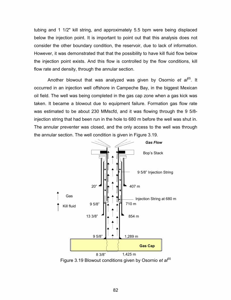
82
tubing and 1 1/2" kill string, and approximately 5.5 bpm were being displaced
below the injection point. It is important to point out that this analysis does not
consider the other boundary condition, the reservoir, due to lack of information.
However, it was demonstrated that that the possibility to have kill fluid flow below
the injection point exists. And this flow is controlled by the flow conditions, kill
flow rate and density, through the annular section.
Another blowout that was analyzed was given by Osornio et al55. It
occurred in an injection well offshore in Campeche Bay, in the biggest Mexican
oil field. The well was being completed in the gas cap zone when a gas kick was
taken. It became a blowout due to equipment failure. Formation gas flow rate
was estimated to be about 230 MMscfd, and it was flowing through the 9 5/8-
injection string that had been run in the hole to 680 m before the well was shut in.
The annular preventer was closed, and the only access to the well was through
the annular section. The well condition is given in Figure 3.19.
Figure 3.19 Blowout conditions given by Osornio et al55
Bop’s Stack
Gas Flow
9 5/8” Injection String
13 3/8” 854 m
20” 407 m
9 5/8” 710 mInjection String at 680 m
9 5/8” 1,289 m
8 3/8” 1,425 m
Gas Cap
Gas
Kill fluid

83
Two methods were considered for calculating the control parameters:
dynamic and momentum kill. Figure 3.20 shows the momentum kill analysis. It
can be seen that the required kill rate to reach the force required to change the
momentum due to the gas velocity to zero at the injection depth was about 68
bpm of seawater. However, the well was successfully controlled with about 19
bpm, a rate very close to that predicted by dynamic kill technique as documented
by the authors55. Therefore, an attempted momentum kill would have required
more horsepower, surface pressure and flow rate than necessary to control the
well.
Figure 3.20 Momentum kill analysis for the offshore blowout described by
Osornio et al55
A hypothetical oil blowout was also analyzed, since the momentum
concept considers a collision between two fluids, and those fluids can be either
0
200
400
600
800
1000
1200
1400
1600
0 100 200 300 400 500 600 700 800 900 1000
Injection String at 680 m.
68 bbl/min55 40
Momentum of the Gas vs Momentum of the Control Fluid
Momentum (lbf)
D e p t h (m)
Momentum of the Gas
Momentum of the kill fluid

84
gas or liquid. Thus, the theory should also apply for a collision between formation
oil and kill fluid.
The information was taken from a real well (tubulars and wellbore
geometry, formation and formation fluid properties, etc).
Figure 3.21 presents the conditions during the hypothetical oil blowout.
The calculated oil flow rate at those circumstances was about 14,400 bpd flowing
up through the wellbore, open hole and casing, and then through the annular
section between the 9 5/8" casing and 5" drillpipe.
Figure 3.21 Hypothetical oil blowout conditions utilizing actual data.
9 5/8” 10,000 ft
8.535” 11,400 ft
PR = 4,600 psi TR = 280 oF k = 2,000 md
Injection String: DP: 5 x 4.808” at 800 ft.

85
After the oil flow rate was estimated, the blowout control was designed
and the kill parameters were calculated employing both the momentum kill and
dynamic kill concepts.
Figure 3.22 presents the momentum kill analysis with the solid line
showing the momentum of the formation fluid through the well. Considering the
oil as incompressible fluid with no gas in solution, it can be seen that the
"momentum" of the oil from the injection depth to the surface is about 5.9 lbf, and
the "momentum" from the injection depth to the bottom is about 3.9 lbf.
Therefore, by utilizing seawater as kill fluid, the required kill flow rate to bring the
well under control under this concept would be around 9.5 bpm.
Figure 3.22 Momentum kill analysis for the hypothetical oil blowout
A conventional dynamic kill analysis was also performed at the
hypothetical oil blowout. Figure 3.23 indicates the results of the system analysis
D e p t h (ft)
0
1,000
2,000
3,000
4,000
5,000
6,000
7,000
8,000
9,000
10,000
11,000
12,000
0 2 4 6 8 10
Momentum of the Formation Oil (lbf)
Momentum
Injection string depth
bpmqkf 5.9�
No matter where the injection point is, the calculated "momentum" kill flow rate is the same.

86
approach for the oil blowout. The dashed line represents the reservoir inflow
performance, and the solid curves stands for the wellbore hydraulics
performance for different kill flow rates of seawater. The bottom curve is the
wellbore hydraulics performance when only formation oil is flowing through the
well and the kill flow rate is 0 bpm. The intersection of this curve with the IPR
curve corresponds to the well condition after all the drilling mud has been
unloaded from the wellbore and a free flowing condition has been reached. For
this blowout, the calculated oil flow rate was 14,400 bpd. Applying this concept,
it can be seen that the required kill rate of seawater to control the well is almost
50 bpm, which is nearly 5 times greater than that given by the momentum
method.
Figure 3.23 Dynamic kill analysis for the hypothetical oil blowout
Bottomhole Flowing Pressure vs Oil Flow Rate
4,400
4,450
4,500
4,550
4,600
4,650
4,700
0 3,000 6,000 9,000 12,000 15,000 18,000 21,000Oil Flow Rate (BPD)
Botto
mho
le F
low
ing
Pres
sure
(psi
a)
IPR WHP
50
40
30
20
10
0 bpm
87
The pressure profile was computed for both 10 bpm for "momentum" kill
and 50 bpm for dynamic kill, and it was found that the bottom hole pressure
generated by the 10 bpm profile was not enough to reach the formation pressure.
However, the pressure profile calculated with the 50 bpm kill rate given by the
dynamic method yielded a bottom pressure equal to the formation pressure,
reducing the implied oil influx rate to zero.
The momentum kill technique indicates that it would be possible to utilize
a kill density equal to the oil density, and a kill rate equal to the well flow rate to
equalize both momentums and to stop the flow. Thus the kill rate would equal to
the formation oil flow rate for any tubular geometry and kill string depth. This
result seems inherently illogical unless there are no flow related pressure losses
in the formation or in the well below the injection point. Therefore, it is expected
that the momentum kill design method in most of the cases will underpredict the
kill rate required for an oil or water blowout.
Another conclusion from this oil well analysis is that the dynamic kill
method is very sensitive to the injection string depth. If the string length
increases, the kill and formation fluid mixture will have more annular section
length to generate both friction losses and hydrostatic head, and vice versa if the
string length decreases. On the other hand, it can be seen in Figure 3.22 that the
momentum concept yields the same kill flow rate, regardless of injection depth,
for the same oil flow rate. However, it is known that if the injection depth
changes, the total hydraulic system also changes, and consequently the kill flow
rate should be different.
3.2.5 Conclusions Regarding the Momentum Method 1. The momentum procedure is supposedly based on Newton's Second Law of
Motion, but it does not consider the external forces (body, tangential, and
normal) in its design calculation. That is, the calculation assumes that only the
deceleration of the kill fluid mass will stop the formation fluid flow and change

88
its direction. However, a complete formulation of Newton's Second Law of
Motion applied to fluids states that the acceleration of the fluid depends
directly on all of the forces in the system. 2. The published2,6,7,8,9 momentum kill procedure does not provide a basis for a
pressure profile analysis. Therefore, the flow directions and velocities after
the collision between the formation and kill fluid and pressures applied to
surface and subsurface equipment are unknown. Therefore, confirmation of
the effectiveness and safety of the method is not possible with the published
method. 3. The analysis of reported8,9 momentum kills is possible with a more
comprehensive hydraulics model as described herein for dynamic kill. The
analysis performed on three actual gas blowouts described by Grace8, 9 and
Osornio et al55 confirmed that a successful kill was expected in each case. It
also showed that the kill rates used in the momentum kills would easily
generate a higher bottomhole pressure than the formation pressure and in
effect were higher than the required to kill the well, except in the ambiguous
case described in reference 8. 4. A study developed for a hypothetical oil blowout indicated that the kill rate
given by momentum concept is not affected by the tubular geometry in the
wellbore or by the injection string depth. That is, for a given oil flow rate and
kill density, the “momentum force” that will supposedly reduce the oil velocity
to zero and displace it downward through the wellbore will be always the
same. It is expected that the momentum kill design method will underpredict
the kill rate necessary for an oil blowout.
89
CHAPTER 4
DYNAMIC SEAL – BULLHEADING METHOD
The previous chapter presented an analysis of the current off - bottom
blowout control methods, and identified some operational and design
shortcomings. In addition, the risk of having more complex blowouts increases
due to deeper, higher pressure and higher technology wells. Therefore, it is
important to investigate different alternatives to regain control in a rapid and
effective way and to minimize blowout consequences.
The primary goal of this research was to develop an engineering
procedure to assist designing and predicting all kill parameters for a successful
and efficient off - bottom kill job by pumping control fluid through an injection
string in the well. The model developed in this dissertation called "dynamic seal -
bullheading" allows the kill parameters such as kill flow rate, kill density, required
kill fluid volume, pumping time, and effect of control depth to be known. The
model also allows the formation fluid influx rate, surface pressure, bottomhole
pressure, and pressure at critical points in the well to be calculated as function of
time. The mathematical procedure was implemented in an Excel spreadsheet
using macros. This chapter describes the analytical models used, the global
solution scheme, and some example applications of the method. 4.1 Principle
The conceptual basis of the dynamic seal - bullheading method involves
two important stages in the control process. First, a dynamic seal has to be
generated at the injection string depth, which will force a portion of the kill fluid to
flow downward from the string depth in a controlled way. Second, this kill fluid
flowing downward will force the remaining formation fluid in the wellbore back
into the permeable zone or other open formation, which is essentially a
bullheading process.

90
A dynamic seal is a hydraulic seal that is developed when the pressure
required to push fluids through a flow path to the surface exceeds the pressure
required for a hydrostatic balance with the formation pressure. It is generated by
pumping kill fluid down through the injection string to establish a mixture of
formation and kill fluids flowing from the injection depth to the surface increasing
the pressure due to hydrostatic head, frictional pressure drop and acceleration at
the injection depth. The pressure depends directly on both kill flow rate and kill
density. Hence the dynamic seal is attained when the pressure at the injection
point depth generated by the pumping conditions is high enough to force the kill
fluid downward.
The dynamic seal generation is schematically illustrated in Figure 4.1,
which presents an off - bottom blowout scenario. Figure 4.1a indicates the initial
well conditions when only formation fluid is flowing in the system. The solid line
denotes the flowing gas pressure profile from the bottom to the surface. The flow
path is through the openhole, casing and annulus. The dashed line represents
the static gas pressure in the injection string.
On the other hand, Figure 4.1b presents the well conditions a few minutes
after the control is started. The solid line, labeled )1(kfq , is the pressure profile
given by the rate, )1(kfq , of a selected fluid density once the pumping operation
has reached steady state conditions. The solid line, labeled )2(kfq , represents the
pressure profile yielded by a higher rate of, )2(kfq , and so on for the line labeled
as )3(kfq . In this illustration, the greatest rate is )3(kfq , the lowest one is )1(kfq , and
an intermediate rate is given by )2(kfq . It can be seen that the bottomhole
pressure increases with the kill rate until the injection pressure is reached. When
the formation fluid just begins to flow into a permeable zone, the dynamic seal
has been attained at the kill string depth. Then those parameters, rate and
density, are the ones needed to achieve the hydraulic seal.

91
Figure 4.1a Initial conditions of the dynamic seal generation
Figure 4.1b Dynamic seal process
Injection Pressure
Flowing pressure profile (open hole/casing/annulus)
Static pressure profile (kill string)
Kill string depth D e p t h
Pressure
Injection Pressure
Pump pressure
)3()2()1( kfkfkf qqq ��
)1(kfq )2(kfq )3(kfq
D e p t h
Pressure
Kill mud

92
Following the concept of dynamic seal - bullheading, once the hydraulic
seal has been reached at the injection string depth, the formation fluid can be
displaced into the permeable formation by the kill fluid. This operation is
practically a bullheading process. The bullheading process is a kill method in
which the kill fluid forces the formation fluid back into the formation. The second
stage of this procedure is schematically illustrated in Figure 4.2.
Figure 4.2a Bullheading process
Injection Pressure
Pump pressure Depth
Pressure
Dynamic seal
Kill mud
Surface kill fluid pump rate
Kill Rate
Minimum rate for dynamic seal
Minimum rate for Bullhead
Minimum rate for dynamic seal bullheading
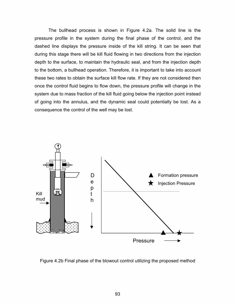
93
The bullhead process is shown in Figure 4.2a. The solid line is the
pressure profile in the system during the final phase of the control, and the
dashed line displays the pressure inside of the kill string. It can be seen that
during this stage there will be kill fluid flowing in two directions from the injection
depth to the surface, to maintain the hydraulic seal, and from the injection depth
to the bottom, a bullhead operation. Therefore, it is important to take into account
these two rates to obtain the surface kill flow rate. If they are not considered then
once the control fluid begins to flow down, the pressure profile will change in the
system due to mass fraction of the kill fluid going below the injection point instead
of going into the annulus, and the dynamic seal could potentially be lost. As a
consequence the control of the well may be lost.
Figure 4.2b Final phase of the blowout control utilizing the proposed method
Injection Pressure
Formation pressure D e p t h
Pressure
Kill mud

94
Figure 4.2b displays the final phase of the control. The solid line
represents the pressure profile in the well in static conditions. This procedure
utilizes only one kill density during the control operation. The chosen fluid density
would be the one that generates a hydrostatic pressure at the bottom between
the formation pressure and the injection pressure, see Figure 4.2b.
It was previously shown that the proposed method considers two
important stages, which were individually considered. Therefore, two models had
to be created: one to obtain the dynamic seal and another to describe the
bullheading operation. In this work the two models were analyzed, built, and
programmed separately; then they were coupled to obtain the final one. 4.1.1 Dynamic Seal Mathematical Model
The dynamic seal mathematical model involves two major components,
the wellbore and the reservoir. These were coupled, since a variation of the flow
conditions in the wellbore will inevitably cause a modification to the reservoir
performance. The link between these two sections was the face of the production
zone.
The dynamic seal analysis considered four sections in the system, three in
the wellbore and one in the reservoir. Figure 4.3 illustrates a typical off - bottom
blowout with the four zones to model the different areas of interest in the system.
Zone 1 represents the producing formation, which produces the uncontrolled flow
of formation fluid toward the surface. Zone 2 is in the wellbore and represents the
section of single-phase, formation fluid, flow from the bottom of the well to the
injection string depth. Zone 3 is also in the wellbore and represents the two-
phase flow generated by the formation fluid and the kill fluid flowing through the
annular section, from the string depth up to the surface once the pumping
operations begin. Finally zone 4 contains the single-phase control fluid flow down
through the kill string.

95
Figure 4.3 Interest zones to model the areas in the system
The mathematical model for each zone is explained in the following sections. 4.1.1.1 Model Assumptions
The following assumptions and considerations have been made in developing
the dynamic seal model. �� The flow system has one-dimensional spatial geometry along wellbore due to
the limited cross sectional size compared with the axial wellbore length
�� The temperature gradient is constant and known
�� The formation fluid is single phase gas or liquid
�� The kill fluid has constant properties
�� Only single phase flow exists below the injection point until a dynamic seal is
achieved
�� The injection rate of the kill fluid is constant
�� No mud moves down into zone 2 until bottomhole pressure exceeds
formation pressure
Zone 3 Two phase flow
(formation and kill fluid) through the
annular section
Zone 2 Single phase flow (formation fluid)
from the bottomhole to the sting depth
Zone 1 producing formation
Zone 4 Single phase flow (kill fluid) into the injection string

96
�� Flow rate of mud moving up annulus is constant after injection pressure is
achieved.
�� Kill is complete when mud is bullhead to the formation face
�� The producing formation is isotropic and the flow is radial 4.1.1.2 Wellbore Model
The wellbore model considers three zones, which were previously defined,
see Figure 4.3. The equations employed to model the flow process in those
zones are the conservation of linear momentum, conservation of mass, equation
of state, gas velocity equation, and fluid and PVT property correlations. The
conservation of linear momentum 34 that is based on Newton's second Law of
motion 14 is given by
gdvf
Lpv
Lv
t�
��� ��
�
���
�
��
�
�
2)()(
22 (4.1)
The Conservation of Mass 34 is represented by
0)()( ��
��
�
� vLt
�� (4.2)
The combination of the above equations gives the well-known pressure gradient
equation, given by
accelft dL
dpdLdp
dLdp
dLdp
��
���
���
�
���
���
�
���
���
�
���
� (4.3)
The derivation of the pressure gradient equation is presented in Appendix
B. The left-hand side term of Equation 4.3 is the total pressure gradient of the
fluid in the interval studied. The first right-hand-side term accounts for frictional
pressure losses due to the viscous shearing stress between the fluid and the

97
wellbore/pipe wall and always causes a drop of pressure in direction of the flow.
It is given in field units by
d
vfdLdp
f 17.772
2�
���
���
� (4.4)
The second right-hand-side term accounts for the hydrostatic pressure of
the fluid and acts in the direction of the gravitational field. It is given by
144�
���
���
�
eldLdp (4.5)
The third right-hand-side component accounts for pressure changes
caused by fluid acceleration; a pressure drop occurs in the direction that the
velocity increases. It is represented by
L
vdLdp
acc �
���
�
���
�
6.9273
2� (4.6)
The friction pressure loss component represented by Equation 4.4
involves the calculation of the friction factor ( f ) which strongly depends on the
rheological model of the fluid, i.e., whether the control fluid follows Newtonian or
non-Newtonian behavior. 4.1.1.2.1 Newtonian Kill Fluids
Newtonian fluids such as water and brines are sometimes used in well
control operations. The primary peculiarity of the Newtonian fluids is that the
shear stress (� ) is directly proportional to the shear rate (�� ). The mathematical
model is given by
��� �� (4.7)

98
where � is the constant of proportionality and is known as the viscosity of the
fluid.
The friction factor in the friction term of the pressure gradient equation has
not been analytically characterized except for laminar, single-phase flow. Hence
it must be calculated by experimental work for turbulent flow. The friction factor is
a function of both Reynolds number ( ReN ) and relative roughness (� ). The
Moody friction factor ( f , dimensionless), which is four times larger than the
fanning friction factor ( f � ), is adopted through this work.
ff �� 4 (4.8)
The procedure to evaluate the friction factor requires knowing whether the
flow is laminar or turbulent. Laminar flow (considered to exist if the Reynolds
number is less than 2,100) is calculated as follows:
Re
64N
f � (4.9)
Turbulent flow has no analytical representation, but several empirical
equations have been proposed. In this work, the friction factor for non-Newtonian
turbulent flow is calculated using the Serghides' equation45. It is an explicit
approximation to the Colebrook's correlation34. Serghides' formula avoids the
iterative solution and gives a maximum deviation of 0.0023%. It is given by
� �2
789
278
7 2
�
��
�
�
��
�
�
��
��
AAAAA
Af (4.10)
where: ���
����
���
Re7
127.3
/log2N
dA �

99
���
����
���
Re
78
51.27.3
/log2NAdA �
���
����
���
Re
89
51.27.3
/log2NAdA �
When the flow is through the annular section, d is computed using the
equivalent circular diameter concept1 which is given by
� �12816.0 ddde �� (4.11)
where:
de = Equivalent diameter (in).d1 = External diameter of injection pipe (in).d2 = Internal diameter of outer pipe or borehole (in).
d1
d2
Figure 4.4 Flow through annular section
The Reynolds number, ReN (dimensionless), is defined by
�
�vdN 124Re � (4.12)
The same equation can be used for flow through pipe or annulus, using d
or ed , respectively.

100
4.1.1.2.2 Non - Newtonian Kill Fluids
During well control operations, it is some times necessary to use a higher
fluid density than water to control the well. Naturally this will depend on the
productive zone properties. The only two ways to obtain those densities are by
using either brines or drilling muds, but due to the cost and simplicity to prepare
them in high densities, the most common kill fluids are muds. A complication is
that those fluids have non-Newtonian behavior. That is, they do not exhibit a
direct proportionality between shear stress and shear rate, making them more
difficult to characterize. The non-Newtonian fluids used in drilling operations are
pseudoplastic, fluids whose apparent viscosity decreases with increasing shear
rate. The Bingham plastic and power law rheological models are most commonly
utilized to represent a pseudoplastic behavior. In this work, the power law model
will be adopted to represent the non-Newtonian behavior of the kill fluid.
The power law fluids, like Newtonian fluids, will flow under any applied
stress. However, as distinct from Newtonian fluids, the shear stress is not
proportional to the shear rate, but to its nth power. It is defined by
nK�� �� (4.13)
This model requires two parameters for fluid characterization1. One of
them is K , consistency index, and is indicative of the pumpability or overall
thickness. The other parameter is n , flow behavior index, and it can be
considered as a measure of the degree of deviation of a fluid from Newtonian
behavior. For 1�n , the Equation 4.13 becomes the Newtonian fluid equation.
The units of the consistency index (K ) depend on the value of n . K has units of
dyne-sn/cm2. In this work, a unit called equivalent centipoise, eq cp, will be used
to represent 0.01 dyne-sn/cm2.
The determination of the flow behavior index ( n ) is computed with the
following equations1:

101
���
����
��
300
600log322.3�
�n
or
���
����
�
��
�
�
��
�
�
�
1
2log
log1
2
NN
n N
N
�
�
(4.14)
On the other hand, the consistency index is calculated as follows
nK511
510 300��
or
� �nN
NK
703.1510�
� (4.15)
The dial readings used in these equations are measured with a standard
Fann viscometer.
For fully developed laminar flow, the friction losses can be predicted by
the Metzner - Reed equations1. For pipe it is given by
n
n
n nd
vKdLdp
����
�
�
����
�
��
�� 0416.0
13
000,144 1 (4.16)
For the annulus the pressure loss gradient is given by

102
� �
n
n
n ndd
vKdLdp
����
�
�
����
�
��
�
� 0208.0
12
000,144 112
(4.17)
Where dLdp is the frictional pressure gradient when laminar flow is present.
The friction factor for turbulent non-Newtonian flow is calculated utilizing
the Dodge and Metzner method34. They suggested an implicit friction factor
equation, which is calculated in an iterative procedure and is given by
2.12
1
Re75.0
395.0log41n
fNnf
n
���
�
�
��
�
��
�
��
���
��
(4.18)
The Reynolds number 67 is calculated utilizing the apparent Newtonian viscosity
a
dvNRM
�
�124Re �
�
(4.19)
Again the internal pipe or borehole diameter is used for pipe flow, and the
equivalent diameter concept using Equation 4.11 is utilized for flow through
annulus. The apparent viscosity 67( a� ) for flow through pipe is given by
� �
� �
����
�
�
����
�
��
��
�
0416.0
13
96 1
1 nv
Kdn
n
a� (4.20)
On the other hand, the apparent viscosity for flow through annular section
is computed by

103
� �� �
� �
����
�
�
����
�
��
�
�
�
0208.0
12
144 1
112 n
vddKn
n
a� (4.21)
The computer program will calculate the frictional pressure losses for both
laminar and turbulent flow. Then, the larger value will be chosen as the correct
one. This will avoid dependence on Reynolds number criteria.
Other parameters and fluid properties such as density, viscosity, and
velocity are required to compute the friction factor and the total pressure
gradient.
In - situ gas density is a function of pressure and temperature and will be
calculated utilizing the real gas law20, which is given by
zTp
gg �� 7.2� (4.22)
Here g� , is the specific gravity of the gas and is given by the ratio of the
molecular weight of the gas ( gM̂ ) to the molecular weight of dry air. It can be
calculated by
96.28
ˆg
g
M�� (4.23)
The gas compressibility factor ( z ) is computed using the Dranchuk &
About - Kassem equation20, which is a fitted equation of state to the data of
Standing and Katz23. It is given by the following equations.

104
� � � �2113
22
11105
287
9
2287
655
44
332
1
1
1
rpr
prrr
prpr
rprpr
rprprprpr
AEXPT
AATA
TAA
TA
TAA
TA
TA
TA
TAAz
��
��
��
���
�
�
��
�
���
��
�
�
��
�
���
��
�
�
��
�
����
��
�
�
��
�
������
(4.24)
���
�
���
��
pr
prr zT
p27.0�
pc
pr ppp �
pc
pr TTT �
26.31318.756 ggpcp �� ���
2745.3492.169 ggpcT �� ���
where the constants 111 AA � are as follows:
01569.0 5339.00700.13265.0
4
3
2
1
�
��
��
�
AAAA
0.1874 -0.73610.5475
-0.05165
8
7
6
5
AAAA
7210.06124.0 1056.0
11
10
9
�
�
�
AAA
The viscosity is utilized for determining the Reynolds number. In this work
the in-situ gas viscosity ( � ) is calculated using the Carr, Kobayashi, and Burrows
correlation23. This correlation takes into account both fluid pressure and
temperature for each calculation. It is given by
� � gg T ��� log1015.610188.810062.210709.1 33651
����
��������

105
The ratio of 1/ �� is evaluated from
� �
� � � �315
2141312
3311
21098
2
37
2654
33
221
1
ln
prprprprprprprpr
prprprprprprpropr
papapaaTpapapaaT
papapaaTpapapaaT
��������
�����������
����
�
�
�
where the constants 150 aa � are given by
05
04
33
12
01
00
103.49803305 102.80860949
10054205228.
1086264054.21097054714.2
1002.4621182
���
��
��
���
��
���
�
�
a
a
a
a
a
a
311
110
09
18
27
16
104.41015512
10.491449251
101.39643306
1093385684.7
1004432413.1
10.60373020 2
�
�
�
�
�
��
���
��
���
���
��
a
a
a
a
a
a
4
15
214
113
212
10.095792636
1003367881.2
1086408848.11039387178.8
�
�
�
�
�
�
a
a
aa
Finally the gas viscosity is obtained by:
��
���
����
�
� TprTpr
g1
1 lnexp�
��� (4.25)
The in-situ gas velocity ( gv ) is defined as
Aq
v gg �
but: ggscdg Bqq � (4.26)
where gB is the gas formation volume factor68 and is calculated from the gas real
law as follows:

106
pzTBg 02829.0� (4.27)
Combining the above expressions and writing the gas velocity in practical units:
pAzTq
v gscdg
7102743.3 �
�� (4.28)
Where A is the flow area, it can be pipe or annular.
Once the kill fluid reaches the injection point, there will be a mixture of the
kill fluid and the formation fluid from the string depth to the surface. Therefore a
two-phase flow model should be used for determining pressure losses.
Kouba33 presented an analytical method that considers homogeneous flow
for calculating the pumping requirements to achieve a dynamic kill. He concluded
that the homogeneous model is very accurate at high flow rates. Fan Jun et al 44
developed a transient on - bottom dynamic model for killing of a single-phase gas
blowout. They also adopted a homogeneous model, since they considered that
the gas flow system is of rather high flow rate at the principal stages in kill
process. This has been proven accurate enough to characterize flow in the mist
flow regime. Oudeman et al.54 designed, executed, and analyzed a full-scale
field test to study how a dynamic kill proceeds in gas wells. They obtained
excellent results with the homogeneous flow model, reportedly because at the
high flow rates encountered in the blowing well, slip between gas and liquid do
not play an essential role, and the refined multiphase flow models did not yield
answers essentially different from the homogeneous model.
In this dissertation, a conventional dynamic kill model was also built
considering homogeneous flow. It was then run with data from the blowout that
occurred in Mobil Indonesia's Arun field32. The results showed excellent
agreement with results from other models 32, 33, 53 that used the same information

107
to calculate the kill parameters, see Table 3.2, even though the model given by
Al-Sheri53 is a rigorous two-phase flow model.
The homogeneous flow pattern was adopted for modeling the dynamic
seal generation phase because it gives reliable results in high flow rates, which
are present during this process. Therefore, the pressure gradient equation
(Equation 4.3) for a two-phase flow mixture becomes
L
vd
vfdLdp mmmmm
t �
�����
�
���
6.927314417.772
22��� (4.29)
where m� , is the mixture density 22, which can be calculated as
����� gkfm �� (4.30)
The volumetric fraction of the control liquid (� )34 also called liquid holdup,
is defined as the ratio of the volume occupied by the liquid component of the total
volume and is given by
gkf
kf
qqq�
�
6.80856.8085
� (4.31)
Here gq is in-situ conditions and is defined by Equation 4.26. The
formation fluid would occupy the remainder of the pipe segment, and for gas
wells it is referred to as gas void fraction or gas holdup. It is obtained by
�� �� 1 (4.32)
The term, mv , in Equation 4.29 is the mixture velocity34, which is defined
as the sum of superficial velocities of both fluid components. It can be estimated
by

108
���
����
� ����
Aqq
vvv kfggkfm
6.8085400,861 (4.33)
The in-situ gas velocity ( gv ) is given by Equation 4.28 and the kill fluid
velocity1 ( kfv ) can be calculated by
2
16.17dq
v kfkf � (4.34)
The Reynolds number of the mixture34 is given by
m
mm dvN
�
�124Re � (4.35)
where m� is the mixture viscosity22 which can be computed by
����� gkfm �� (4.36)
Again, the internal pipe or borehole diameter is used for pipe flow, and the
equivalent diameter concept in Equation 4.11 is utilized for flow through annulus. The in-situ gas viscosity is given by Equation 4.25. 4.1.1.3 Reservoir Model
Another major section that is involved in the dynamic seal model is the
reservoir, shown as zone 1 in Figure 4.3. As the conditions change in the
wellbore, the producing zone will inevitably respond. In well control operations,
the desired response is a decrease in the formation fluid influx rate. Therefore, a
reservoir model should be coupled to the wellbore.
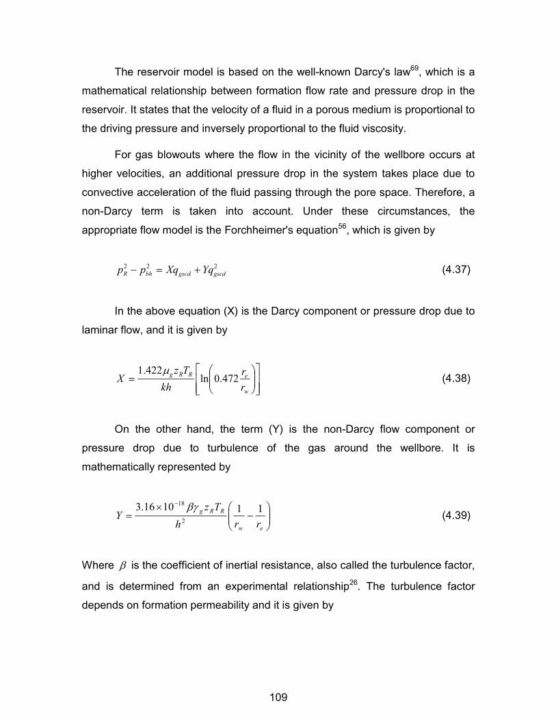
109
The reservoir model is based on the well-known Darcy's law69, which is a
mathematical relationship between formation flow rate and pressure drop in the
reservoir. It states that the velocity of a fluid in a porous medium is proportional to
the driving pressure and inversely proportional to the fluid viscosity.
For gas blowouts where the flow in the vicinity of the wellbore occurs at
higher velocities, an additional pressure drop in the system takes place due to
convective acceleration of the fluid passing through the pore space. Therefore, a
non-Darcy term is taken into account. Under these circumstances, the
appropriate flow model is the Forchheimer's equation56, which is given by
222gscdgscdbhR YqXqpp ��� (4.37)
In the above equation (X) is the Darcy component or pressure drop due to
laminar flow, and it is given by
���
�
���
����
�
�
w
eRRg
rr
khTz
X 472.0ln422.1 �
(4.38)
On the other hand, the term (Y) is the non-Darcy flow component or
pressure drop due to turbulence of the gas around the wellbore. It is
mathematically represented by
���
����
��
�
�
ew
RRg
rrhTz
Y 111016.32
18 �� (4.39)
Where � is the coefficient of inertial resistance, also called the turbulence factor,
and is determined from an experimental relationship26. The turbulence factor
depends on formation permeability and it is given by

110
k
710�� for mdk 000,5� (4.40)
and
35.1
101055.3k�
�� for mdk 000,5� (4.41)
The gas formation properties in Equation 4.38 and 4.39 are calculated at
reservoir conditions.
Solving the quadratic equation, Equation 4.37, it is possible to compute
the deliverability potential of the reservoir as a function of differential pressure
between the face formation and the producing formation limits.
� �
YppYXX
q bhRgscd 2
4 222����
� (4.42)
It can be seen in Equation 4.42 that the gas flow rate is a function of the
difference between reservoir pressure and bottomhole pressure, formation
properties, formation fluid properties, and flow turbulence 4.1.1.4 Formation Fluid Rate Determination
The formation fluid flow rate is estimated initially when the well has been
completely unloaded of all the drilling mud and free flowing equilibrium conditions
have been reached. That is, only formation fluid is flowing in the system from the
reservoir to atmosphere. Under this situation, the mathematical relationship
between the wellbore and the producing zone yields the maximum formation flow
rate that is possible given the well geometry. These conditions are considered as
the initial conditions of the well control procedure.

111
The formation fluid flow rate depends on two important components, the
reservoir inflow performance (IPR) and the wellbore hydraulics performance
(WHP), also called inflow and outflow performance, respectively.
The IPR is the relationship between the production rate from the reservoir
and bottomhole pressure and is a measure of the formation's capacity to produce
to the wellbore. In this work, the IPR will be estimated by solving Equation 4.37
for the bottomhole pressure, in the form shown as Equation 4.43
22
1822 111016.3
472.0ln422.1
gscdew
RRggscd
w
eRRgRbh q
rrhTz
qrr
khTz
pp��
���
��
���
��
���
�
��
��
���
��
���
��
���
���
���
��
� ���
(4.43)
The formation fluid properties such as the gas deviation factor ( Rz ) and
gas viscosity ( g� ) are calculated with Equations 4.24 and 4.25, respectively.
Then several gas flow rates are assumed and the bottomhole pressure is
calculated for each specific rate employing Equation 4.43. The resulting reservoir
inflow performance curve is plotted on a graph of gas flow rate versus
bottomhole pressure.
On the other side, the WHP is the relationship between the production rate
and the bottomhole pressure generated by that rate flowing to the surface
through the wellbore. In this work, the WHP at the initial conditions with only gas
flowing in the system will be calculated utilizing the Cullender and Smith
equation21, which is given by
dp
Tzp
LH
dfq
Tzp
L s
bh
p
p gscd
g
000,11667.0356.53
000,12
5
���
���
��
��
���
�
��
(4.44)

112
This is the most widely used method to calculate flowing bottomhole
pressure in gas wells34. The Cullender and Smith method makes no simplifying
assumptions for the variation of temperature and gas deviation factor in the
wellbore. Consequently, the procedure is more accurate than other proposed
methods. Equation 4.44 can be solved applying the trapezoidal rule for numerical
integration34, 64.
When gas flow is through an annular section, the following equation for
the diameter is used in Eq. 4.44:
� �� �221
2212
5 816.0 ddddd ��� (4.45)
where 2d and 1d are schematically shown in Figure 4.4.
The friction factor ( f ) and gas deviation factor ( z ) are calculated with
Equations 4.10 and 4.24 respectively. Again several gas flow rates are assumed,
and the bottomhole pressure is calculated for each specific rate, employing
Equation 4.44. The resulted wellbore hydraulics performance curve is
superimposed on the same graph as the IPR curve.
The simultaneous solution of the reservoir inflow performance and
wellbore hydraulics performance is given at the intersection point between the
curves generated by those Equations 4.43 and 4.44, representing the natural
flow point for that system. Thus, the conditions at that intersection point yield
both the formation fluid flow rate and the flowing bottomhole pressure when only
formation fluid is flowing through the wellbore.
Figure 4.5 displays a typical relationship between the IPR and the WHP. It
can be seen that the intersection point is the natural flow point of the well and
gives both the bottomhole pressure and the formation fluid flow rate when only
formation fluid is flowing.

113
Once the gas flow rate is known, it is employed in Equation 4.44, and the
pressure profile in the system from the bottom to the surface is estimated.
Chapter 5 will present a real calculation of these parameters.
Figure 4.5 Formation fluid rate and bottomhole flowing pressure determination 4.1.1.5 Global Solution Scheme
The wellbore model and the reservoir model were coupled at the sand
face to obtain a global solution as a basis for computing the flow conditions in the
wellbore during the control process as a function of axial position at selected
times. The solution scheme for applying the dynamic seal mathematical model
utilizes a series of fully steady states solutions assuming that a given steady
state flow condition exists for the time for the mixture creating those conditions to
reach the surface. By employing this approach, the approximate effect of time
WHP
IPR
F B H P
Formation Fluid Flow Rate
Natural flow point
Formation fluid flow rate
Bottom hole pressure

114
can be included in the process. As a consequence, the kill fluid volume required
to reach the dynamic seal can be obtained.
The solutions using this scheme predict the pressure behavior at any point
in the wellbore and in the injection string as a function of spatial location along
the flow path at selected times. The solution requires the specification of initial
and boundary conditions to solve the flow equations. 4.1.1.5.1 Initial Conditions
The initial conditions are determined when the formation fluid has
completely unloaded the well of all the drilling fluid. Under this circumstance, only
formation fluid is flowing in the system, and the equilibrium conditions have been
reached. At this point, the formation flow rate and pressure profile from the
surface to the bottom are calculated in the system as described in the previous
section. Thus it is assumed that the blowout well has been flowing at a constant
rate for a period of time such that steady state flow has been achieved inside the
wellbore before and at the instant that the killing operation starts.
The wellbore is discretized into cells or grids of equal length along the
length of the well. Hence, knowing the formation fluid flow rate, flowing bottom
hole pressure, surface pressure, geothermal temperature gradient, and cell
length, the initial conditions along the wellbore can be estimated.
The initial distribution of density, viscosity, flow rate, velocity, and pressure
gradient along the axial position can be computed utilizing Equations 4.22, 4.25,
4.26, 4.28 and 4.3, respectively, and a pressure traverse procedure as discussed
in the next section. The process of calculating the initial distribution of conditions
is schematically presented in Figure 4.6.
The pressure traverse procedure is applied at each cell and marching
downward until reaching the bottom of the well. The velocity is corrected for
changes in cross sectional area.

115
Figure 4.6 Determination of the initial conditions
4.1.1.5.2 Boundary Conditions With a surface blowout in process, it is assumed that the pressure and
temperature conditions at the surface are known. So one known boundary
condition is at the surface during the entire dynamic seal process. Another
boundary is at the bottom of the well, where the wellbore is connected with the
producing formation with known fluid properties and rock properties. Therefore,
after the kill begins and a new bottomhole pressure is obtained by applying the
pressure traverse procedure started at the surface, the reservoir mathematical
model can be used to give a new formation fluid rate. This will be utilized to
Pressure Profile
Flow Direction
D+n
D+1
D
.
.
.
.
.
.
1
2
t=0
BC
Surface
IPR
WHP
BHFP
Formation Fluid Flow rate
Gas flow rate determination
De p t h
Pressure
n

116
obtain the new distribution of densities, viscosities, velocities, flow rates, fluid
fractions, and pressure gradient for a given time step.
The global solution procedure to describe the dynamic seal process is as
follows. After the formation fluid rate and the pressure profile in the system have
been computed, the initial fluid flow conditions throughout the wellbore are
calculated, as described in the initial conditions section, utilizing the surface
boundary condition. Then, the control operations begin by pumping a control fluid
of a given density and with constant properties at a given rate downward through
the injection string or down the annulus if the blowout is up the inner string.
The calculation procedure starts when the kill fluid is at the injection depth,
that is just after the first droplet of liquid leaves the injection string and flow to the
annulus. However, the time to fill the injection string is considered in the process.
Therefore, the predictions of pressures while establishing a dynamic seal begin
at the time required to fill the drillstring. Time zero or time at zero seconds is
when the pumping operations just begin and the kill fluid is pumped into the
injection string at the surface.
The dynamic seal model performs the calculation of the time based on the
mixture velocity. That is, if we know the cell length and the mixture velocity the
program calculates the time required to travel from one cell to other. This
procedure is performed at each cell until the kill fluid fills completely the annular
section. The program then sums these times to obtain an estimate of the time
required for fluids to reach the surface after a change in fluid input rates at the
injection point.
For the case of a blowout up the annulus, the calculation procedure starts
at the surface of the annular section considering the initial formation fluid rate
and the kill fluid rate, expressed at standard conditions, as constant and equal in
each cell. Then the pressure traverse for each cell is applied downward, using
the wellbore mathematical model given in the earlier section, until it reaches the
bottomhole. The fluid flow conditions along the wellbore and the bottomhole
pressure can be determined for a specific time step. With the new bottomhole

117
pressure, a new formation fluid rate is calculated utilizing the reservoir model as
the boundary condition equation. Employing the new formation fluid rate, and the
kill rate, the whole procedure is repeated to obtain the flow conditions, pressure
gradient, and a formation fluid rate for a new time step. This process is
schematically presented in Figure 4.7.
Another flow condition is given for the injection string since single-phase
kill fluid is flowing downward through it after the control starts. The pressure
condition in the tubing and at the surface is obtained utilizing the pressure at the
injection depth as a starting point. Then the upward pressure traverse calculation
for single-phase flow is applied until reaching the surface. This procedure is also
repeated for each time step.
Figure 4.7 Wellbore conditions after the first time step is taken
BCBC Injection string
t = 1 t =0
Kill fluid
Flow rate in annulus at t = 1
� � kftg qq ��0
Initial conditions
Casing
At this pressure a new formationrate is calculated that is applied asrate for solution at t = 2

118
4.1.1.5.3 Pressure Traverse Calculation
The pressure traverse calculation for a two-phase flow is a procedure that
calculates the pressure gradient along the wellbore22. It employs the pressure
gradient equation for a two-phase flow mixture (Equation 4.29) as well as the
multi-phase flow properties given from Eq 4.30 to Eq 4.36.
The procedure is started at the top after applying the boundary conditions
and marches downward over small length increments, considering the pipe
geometry changes, until the bottom of the well is reached. The mixture properties
are evaluated at average pressure and temperature in small increments. Then
the pressure gradient is iteratively computed for each cell until a tolerance value
of 0.00001 psi on the upstream pressure is attained. The following procedure
explains the pressure traverse calculation to obtain the pressure gradient along
the wellbore. The procedure is also shown as a flow chart in Figure 4.8. 1. Taking the surface as starting point ( 0L ), compute fluid properties at surface
conditions and select a length increment ( L� ). 2. Estimate the temperature increment ( T� ) corresponding to the length
increment ( L� ). 3. Compute the pressure increment ( 0p� ) corresponding to the length increment
( L� ) using the pressure gradient equation (Equation 4.29) and flow
properties calculated in step 1. 4. Find the average temperature and pressure in the increment. 5. Calculate the fluid and PVT properties at the average temperature and
pressure computed in step 4. 6. Compute the pressure gradient ( Lp �� / ) in the increment utilizing the fluid
and PVT properties obtained at average temperature and pressure
determined in step 5 and the pressure gradient equation (Equation 4.29).
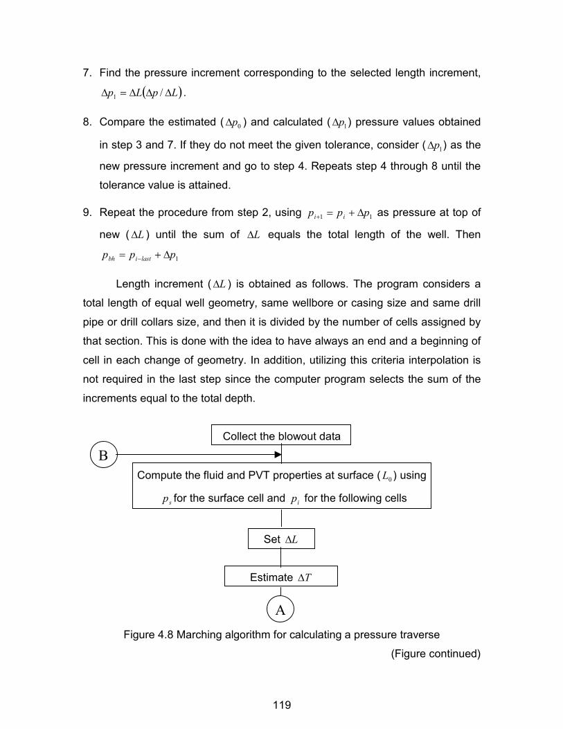
119
7. Find the pressure increment corresponding to the selected length increment,
� �LpLp ����� /1 . 8. Compare the estimated ( 0p� ) and calculated ( 1p� ) pressure values obtained
in step 3 and 7. If they do not meet the given tolerance, consider ( 1p� ) as the
new pressure increment and go to step 4. Repeats step 4 through 8 until the
tolerance value is attained. 9. Repeat the procedure from step 2, using 11 ppp ii ���
� as pressure at top of
new ( L� ) until the sum of L� equals the total length of the well. Then
1ppp lastibh ����
Length increment ( L� ) is obtained as follows. The program considers a
total length of equal well geometry, same wellbore or casing size and same drill
pipe or drill collars size, and then it is divided by the number of cells assigned by
that section. This is done with the idea to have always an end and a beginning of
cell in each change of geometry. In addition, utilizing this criteria interpolation is
not required in the last step since the computer program selects the sum of the
increments equal to the total depth.
Collect the blowout data
Compute the fluid and PVT properties at surface ( 0L ) using
sp for the surface cell and ip for the following cells
Set L�
Estimate T�
Figure 4.8 Marching algorithm for calculating a pressure traverse
(Figure continued)
A
B
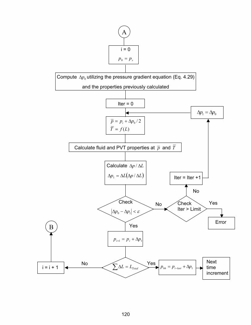
120
i = 0
spp �0
Compute 0p� utilizing the pressure gradient equation (Eq. 4.29)
and the properties previously calculated
Iter = 0
)(2/0
LfTppp i
�
���
Calculate fluid and PVT properties at p and T
Calculate Lp �� /
� �LpLp ����� /1
Check
����� 10 pp
11 ppp ii ����
� �� TotalLL
Next time increment
Yes
Yes
Check Iter > Limit
Iter = Iter +1
No
No
01 pp ���
Yes
Error
i = i + 1 No
1ppp lastibh ����
B
A

121
4.1.2 Bullheading Mathematical Model
During the off - bottom blowout control process that is proposed herein,
two important stages take place that are linked. The model for each stage was
analyzed, built, and programmed independently; then the models were coupled
to obtain the final model. The previous section described the model for the
dynamic seal and this part will focus on the bullheading model.
Once a dynamic seal is achieved at the injection string depth, the
formation fluid can be displaced into an open formation by the kill fluid. This
operation is practically a bullheading process. Bullheading is a kill method in
which the kill fluid forces the formation fluid back into an open formation.
Therefore, a bullheading mathematical model should be developed for the
blowout control method proposed herein.
Due to the fact that the available information in the oil industry about the
bullheading process is limited, a complete bullheading mathematical model was
developed in this dissertation to compute all the kill parameters such as kill rate,
kill density, and kill volume. The model also calculates the surface pressure, the
pressure and position of the kill fluid - formation fluid interface, and bottomhole
pressure, as a function of time during the bullheading process.
The bullheading mathematical model considers three zones during the
bullhead process, two in the wellbore below the injection point and one in the
reservoir.
Figure 4.9 shows a typical bullheading scenario and the zones used to
model the system. Zone 1 represents a permeable formation, into which the
formation fluid, either gas, oil, or water, is flowing from the wellbore. Zone 2 is in
the wellbore and contains the single-phase formation fluid. Zone 3 is the single-
phase kill fluid that is displacing the formation fluid downward.

122
Figure 4.9 Interest zones to model the areas of the bullheading process
4.1.2.1 Model Assumptions
The bullheading model assumptions are almost the same as for the
dynamic seal model in section 4.1.1.1. The additional considerations in this
model are the following: �� A single-phase, gas, oil, or water containing no solids is injected into the
formation.
�� The injected fluid is flowing outwards radially into the formation. 4.1.2.2 Formation Fluid Removal Efficiency
An extremely important factor in this technique is the efficiency of removal
of influx. If a considerable amount of gas remains in the wellbore, the well may
unload and blow out again. The reason for poor removal efficiency is that the kill
mud bypasses the gas during the displacement operation. It has been found that
this phenomenon is dominated by kill fluid velocity.
Kill mud
Formation fluid
Zone 1 Permeable formation
Zone 3 Single phase flow (kill fluid) from the injection depth to
the interface
Zone 2 Single phase flow (formation
fluid) from the interface to the bottomhole
Interface (kill fluid - formation fluid)

123
Koederitz35 performed a study of the bullheading process at the LSU
Petroleum Engineering Research and Technology Transfer Laboratory. The
experiments were conducted in a full-scale, cased well using either water or low
viscosity drilling mud as bullheading fluids and gas the formation fluid. A
schematic of the research well is shown in Figure 4.10. The main objective of the
research was to investigate the removal efficiency, defined as the fraction of gas
removed from the wellbore during the operation, for the bullhead method.
PC
Figure 4.10. Configuration of the research well (after Koederitz35)
The general procedure during the experiments was to circulate the well to
ensure consistent liquid properties and that no gas was entrained in the system.
Then, a known volume of gas was placed at the top of annulus section. The
chosen liquid was then pumped at the selected rate downward through the
annulus, displacing the gas to the bottom of the well. Simultaneously, all the
parameters were monitored. The pumps were stopped and the well shut in.
Finally, the removal efficiency was calculated from the initial and final remaining
gas volumes in the well.
Casing: 7", 38 lb/ft at 1,994 ft. Tubing: 2 3/8", 4.7 lb/ft at 1,903 ft.

124
A total of twelve experimental runs were completed, consisting of seven
using water and five using low viscosity mud as the bullheading fluid. Two
different bottomhole pressures, 2000 and 3000 psi, were maintained during the
experiments. Five pump rates were also utilized, ranging from 12.5 gpm to 50
gpm.
Figure 4.11 shows the removal efficiencies for the experiments as a
function of average annular velocity based on the injection rate, with the runs
grouped by fluid type and bottomhole pressure.
Figure 4.11. Removal efficiency (after Koederitz35)
It can be seen from the above plot that removal efficiency increases with
increasing injection rate. Excellent gas removal is reached at an average velocity
of 0.35 ft/sec with low-viscosity mud and 0.7 ft/sec with water. Also it is possible
to note that bottomhole pressure value does not substantially affect the removal
efficiency once the optimum average velocity is attained.
Removal Efficiency (%)
Average Annular Velocity (ft/sec)
0
10
20
30
40
50
60
70
80
90
100
0 0.1 0.2 0.3 0.4 0.5 0.6 0.7 0.8
Water, 2000 BHP Water, 3000 BHP
Low-vis mud, 2000 BHP Low-vis mud, 3000 BHP

125
Koederitz35 also computed the bubble rise velocities, the velocity
difference between the gas and liquid phase. Those velocities were calculated
using the Harmathy equation.47 Figure 4.12 shows the calculated bubble rise
velocity as a function of annular velocity. Gas and liquid velocities are defined as
positive in the downward direction.
Figure 4.12. Gas bubble rise velocities (after Koederitz35)
Figure 4.12 shows that the bubble rise velocity tends to be positive as the
injection rate increases. Once the average downward water velocity of 0.7 ft/sec
is reached, the gas bubble rise velocity becomes essentially zero, and therefore
the gas will go down at the same velocity as the kill fluid.
Figure 4.13 presents the removal efficiencies for the experimental runs
plotted versus the calculated gas bubble rise velocity. Note that gas bubble rise
velocity is positively correlated with removal efficiency. And a complete removal
Average Annular Velocity (ft/sec)
Bubble Rise Velocity (ft/sec)
-0.50
-0.40
-0.30
-0.20
-0.10
0.00
0.10
0 0.1 0.2 0.3 0.4 0.5 0.6 0.7 0.8
Water, 2000 BHP Water, 3000 BHP

126
of gas occurred as gas bubble rise velocities approach zero. In other words,
when the water reaches an average downward velocity of 0.7 ft/sec, the gas is
completely removed or displaced from the wellbore by water. This indicates that
the gas as a whole is flowing downward with the bullheading fluid.
Figure 4.13. Relationship between bubble rise velocity and removal efficiency
(after Koederitz35)
Koederitz35 also used a multiple regression analysis to develop a
predictive method for removal efficiency during bullheading operations. The best-
fit model found for the removal efficiency (R2 = 0.8872) contained only two of the
dependent variables (fluid type and injection rate). It can be seen in Figure 4.11
that the bottomhole pressure has an insignificant effect in the removal of gas.
Hence it was neglected in the model. The resulting model was the following:
0
10
20
30
40
50
60
70
80
90
100
-0.5 -0.4 -0.3 -0.2 -0.1 0 0.1
Removal Efficiency (%)
Water, 2000 BHP
Bubble Rise Velocity (ft/sec)
Water, 3000 BHP

127
IVELFLRE ������ 3.2719.754.161
Where: RE = Removal efficiency, %.
FL= Injection fluid type, 1 for water and 2 for mud.
IVEL = Injection velocity, ft/sec. 4.1.2.3 Mathematical Derivation
A bullheading model has been developed in this dissertation to predict and
understand the bullheading process. In addition, the required kill parameters for
effective bullheading such as kill density, kill rate, kill fluid volume, bottomhole
pressure, surface pressure, interface pressure and position, and gas rate flowing
into the formation can be computed as function of time using the model.
The mathematical model takes into account the compression of the
formation fluid, which is assumed to behave as a gas, by a known volume of an
incompressible kill fluid, as well as the flow of the formation fluid from the
wellbore into an open formation. It also considers frictional and hydrostatic
pressures for both formation gas and kill fluid in the wellbore.
The general scenario of a bullheading operation is presented in Figure
4.9. It can be seen that before the operation starts, the well is filled with gas.
Then kill fluid is pumped into the well, compressing and reducing the gas volume
so pressure at the bottom is increasing from both gas compression due to
volume reduction and liquid column accumulation. The liquid pumping proceeds
until eventually the formation pressure of a permeable zone is reached. At this
moment, the bottomhole pressure has reached the injection pressure for that
formation and a reservoir model is then included in the process, since there will
be flow from the wellbore into whichever open formation's injection pressure has
been reached. This flow rate will depend on the formation and formation fluid
properties as well as the bottomhole pressure. As the pumping operations
continue, the gas is displaced into the formation and the surface pressure
simultaneously decreases. The process is completed when all the formation gas
128
is displaced into the open formations and the hydrostatic pressure of the kill fluid
is enough to balance or exceed the formation pressure.
It has already been noted that when the formation fluid is gas,
compressibility must be considered. The isothermal gas compressibility
differential equation, which relates the change in volume and pressure due to gas
compressibility for an initial gas volume is used. The gas compressibility equation 65 is mathematically represented by
gi cVdV
dp�
�
1 (4.46)
Equation 4.46 describes the change in pressure ( dp ) that the gas
undergoes as the volume changes (dV ), which is basically what happens in a
bullhead operation as the initial gas volume ( iV ) is compressed. Therefore, the
gas compressibility ( gc ) plays an important role during this process.
The change in volume (dV ) is given by the difference between the volume
of kill fluid pumped into the well ( kfV ) and the volume of gas that has flowed into
an open formation ( gV ). This is analytically given by
gkf VVdV �� (4.47)
In order to introduce time in the process, this volume can also be related
to the difference between the kill fluid rate, ( kfbq ), that is pumped into the well and
the gas ( gbq ), that is flowing into the formation over the period of one time step.
This relation is
� �dtqqdV gbkfb �� (4.48)
129
Substituting Equation 4.48 in Equation 4.46
� �
gi
gbkfb
cVqq
dtdp
�
�
� (4.49)
Equation 4.49 requires a mathematical expression to model the gas flow
into the formation as function of time. Therefore, in this work the unsteady state
flow equation in an infinite-acting reservoir will be utilized24,64. It is given by
���
�
���
��
��
��
�
�� 23.3log
6.1622wtg
gggbR rc
ktkhBq
pp��
� (4.50)
Due to the fact that in this process the flow rate ( gbq ) is considered
positive when the flow is from the wellbore to the reservoir, the above equation
becomes
���
�
���
��
��
��
�
�� 23.3log
6.1622wtg
gggbR rc
ktkhBq
pp��
� (4.51)
Rearranging the above equation
� �
���
�
���
��
��
��
�
��
23.3log6.162 2wtg
gg
Rgb
rcktB
ppkhq
���
(4.52)
Equation 4.52 represents the unsteady state flow in an infinite-acting
reservoir. The gas properties ( gB , RB/Mscf and g� ) are evaluated at the
reservoir pressure ( Rp ) and the reservoir properties such as permeability ( k ),
porosity (� ), total compressibility ( tc ), thickness (h ) and wellbore radius ( wr ) are
considered constant during the process. Therefore, the only time dependent

130
variables are the flowing bottomhole pressure )(tp and time ( t ). Therefore,
equation 4.52 can be represented as follows
� �Rgb ptptCq �� )()( (4.53)
Substituting Eq. 4.52 and 4.53 in Eq. 4.49:
� �
� �
gi
Rkfb
gi
wtggg
Rkfb
cVptptCq
cV
rcktB
ppkhq
dtdp
�
���
�
���
�
���
�
�
���
�
���
���
���
��
��
�
�
��
�
�
��
�)()(
23.3log6.162 2���
(4.54)
Rearranging Eq 4.54:
� �
gi
Rkfb
cVptCtptCq
dtdp
�
��
�
)()( (4.55)
The above differential equation represents the bottomhole pressure change
as a function of time during a bullheading operation. It was solved, utilizing the
power series method, and the solution is given by
� � � �� � � �
� � � �
� � � �
� � � � nng
ni
Rkfbn
gi
Rkfb
gi
Rkfb
gi
Rkfb
gi
Rkfb
gi
Rkfb
gi
Rkfb
gi
Rkfb
tcV
ptCptCqtCn
tcV
ptCptCqtC
tcV
ptCptCqtCt
cVptCptCqtC
tcV
ptCptCqtCt
cVptCptCqtC
tcV
ptCptCqtCt
cVptCptCq
ptp
)()0()()(!
1)()0()()(5040
1
)()0()()(7201)()0()()(
1201
)()0()()(241)()0()()(
61
)()0()()(21)(0)(
0
17
77
6
666
55
55
4
444
33
33
2
222
��
��
��
�
��
�
��
�
��
�
��
�
��
�
��
��
�
���
(4.56)

131
Here )(tp represents the flowing bottomhole pressure at time t , )0(p is
the pressure at time zero, and )(tC is the gas flow rate into the productive zone
per psi of pressure difference, called in this work "flow coefficient", it is
represented by
� �
���
�
���
��
��
��
�
�
��
23.3log6.162
)(
2wtg
gg
R
gb
rcktB
khpp
qtC
���
(4.57)
The flow coefficient )(tC is changing constantly since it depends on time.
The time ( t ) is the time since injection of formation fluids began. It is calculated
utilizing the time at the previous step plus t� , which is the selected time
increment or time step. Note that this time is only a portion of the total time for
the overall kill process because it only begins when the dynamic seal is
achieved. Several time steps from 10 to 60 sec were used to analyze the results
given by the above equations. It can be concluded that the results for the
bullheading period are not affected by the time step size since in all the cases
they were the same. 4.1.2.4 Global Solution Procedure
Equation 4.56 gives the bottomhole pressure as a function of time during a
bullheading operation, but in order to solve the equation, the flow coefficient (C )
and the gas compressibility ( gc ) should be estimated.
Once the time step ( t� ) is defined, the gas properties ( gB , RB/Mscf and
g� ) in Equation 4.57 can be calculated utilizing Equations 4.27 and 4.25,
respectively. Therefore, the flow coefficient (C ) can be calculated.
On the other hand, the gas compressibility ( gc ) in Eq. 4.56 is calculated for each time step utilizing the Mattar, Brar, and Aziz expression20:

132
pc
rg p
cc � And
� �
� �� � ��
�
�
��
�
�
���
��
pr
pr
Trr
Tr
prprr zz
z
Tzpc
��
�
//1
/27.012 (4.58)
where:
� �� � � �211
2211
2113
104287
9
287
655
44
332
1
exp125
2
rrrpr
rpr
prpr
prprprprprprprTr
AAATA
TA
TAA
TA
TAA
TA
TA
TA
TAAz
pr
����
�
��
������
�
�
��
�
���
��
�
�
��
�
����
��
�
�
��
�
�������
�
����
�
���
�
���
��
pr
prpr zT
p27.0�
26.31318.756 ggpcp �� ���
26.31318.756 ggpr
pp�� ��
�
2745.3492.169 ggpr
TT�� ��
�
The constants 111 AA � are shown below.
01569.0 5339.00700.13265.0
4
3
2
1
�
��
��
�
AAAA
0.1874 -0.73610.5475
-0.05165
8
7
6
5
�
�
�
�
AAAA
7210.06124.0 1056.0
11
10
9
�
�
�
AAA
Then, utilizing the selected time step, the computed flow coefficient (C )
and the gas compressibility ( gc ), the bottomhole pressure can be estimated
utilizing Equation 4.56 as a function of time.

133
Once the bottomhole pressure is known, it is possible to compute the
pressure profile (bottom up) along the formation gas from the bottom to the kill
fluid - formation gas interface utilizing the Cullender and Smith equation21, which
is given by
dp
Tzp
LH
dfq
Tzp
L int
bh
p
p gsc
g
000,11667.0356.53
000,12
5
���
���
�
��
���
�
��
(4.59)
Equation 4.59 considers the change in the pressure gradient due to
friction and due to hydrostatic head of the gas.
After that, the pressure from the interface to the injection string depth is
computed utilizing the following equation:
� �skfinterfacesd ppp ��� (4.60)
where: � � � � � �fkfelkfskf ppp ����� (4.61)
The change in pressure due to frictional pressure losses of the kill fluid is
given by
d
vfdLdp kfkf
f 17.772
2�
���
���
� (4.62)
And � � kff
fkf LdLdpp ��
�
���
���
And the change in pressure due to elevation of the kill fluid is represented by
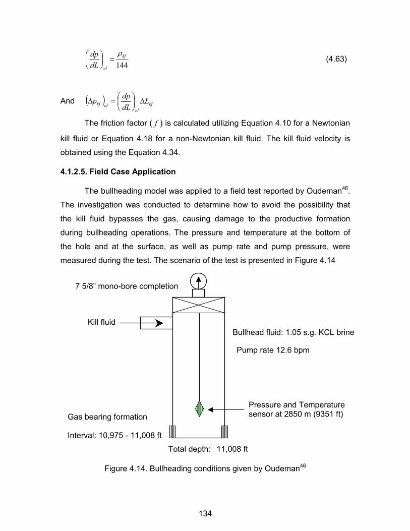
134
144kf
eldLdp �
���
���
� (4.63)
And � � kfel
elkf LdLdpp ��
�
���
���
The friction factor ( f ) is calculated utilizing Equation 4.10 for a Newtonian
kill fluid or Equation 4.18 for a non-Newtonian kill fluid. The kill fluid velocity is
obtained using the Equation 4.34. 4.1.2.5. Field Case Application
The bullheading model was applied to a field test reported by Oudeman46.
The investigation was conducted to determine how to avoid the possibility that
the kill fluid bypasses the gas, causing damage to the productive formation
during bullheading operations. The pressure and temperature at the bottom of
the hole and at the surface, as well as pump rate and pump pressure, were
measured during the test. The scenario of the test is presented in Figure 4.14
Figure 4.14. Bullheading conditions given by Oudeman46
7 5/8” mono-bore completion
Pressure and Temperature sensor at 2850 m (9351 ft)
Kill fluid
Total depth: 11,008 ft
Gas bearing formation Interval: 10,975 - 11,008 ft
Bullhead fluid: 1.05 s.g. KCL brine Pump rate 12.6 bpm
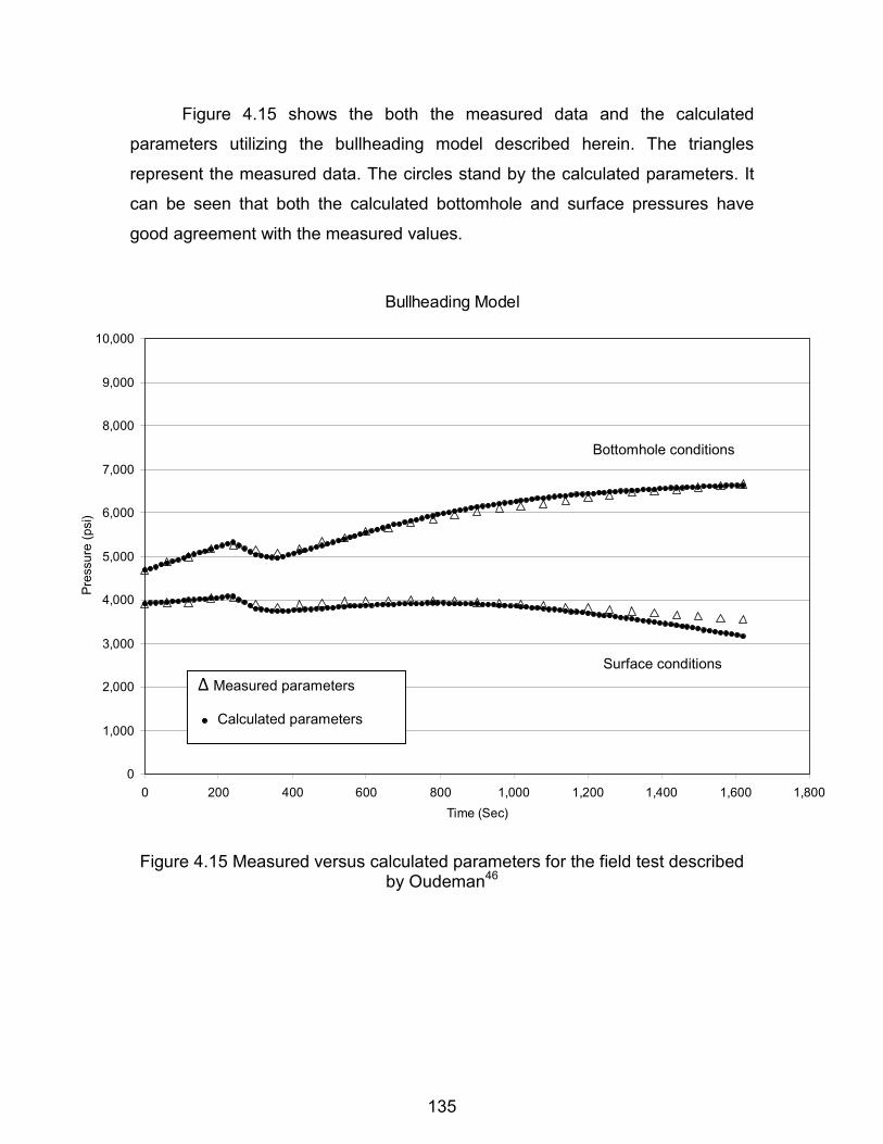
135
Figure 4.15 shows the both the measured data and the calculated
parameters utilizing the bullheading model described herein. The triangles
represent the measured data. The circles stand by the calculated parameters. It
can be seen that both the calculated bottomhole and surface pressures have
good agreement with the measured values.
Figure 4.15 Measured versus calculated parameters for the field test described by Oudeman46
Bullheading Model
0
1,000
2,000
3,000
4,000
5,000
6,000
7,000
8,000
9,000
10,000
0 200 400 600 800 1,000 1,200 1,400 1,600 1,800Time (Sec)
Pres
sure
(psi
)
∆ Measured parameters Calculated parameters
Bottomhole conditions
Surface conditions
136
CHAPTER 5
DYNAMIC SEAL - BULLHEADING PROGRAM AND APLICATIONS
The two models, dynamic seal and bullheading that were defined,
developed, and programmed separately in the previous chapters were coupled to
obtain the proposed model for "dynamic seal - bullheading". Then, it was
implemented in a computer program to assist in off - bottom blowout control
analysis and design. In addition, the computer program may be employed to
investigate different control options including kill fluid type and properties,
injection string geometry and depth, and pump rates, as well as different
formation fluid and rock properties. This capability can be used to help determine
the most appropriate kill approach for a given set of conditions.
The computer program also includes the conventional off - bottom
dynamic kill model, which is based on the steady state analysis approach and
considers that only formation fluid exists below the injection point. Consequently,
the dynamic method and the proposed method can be compared for the same
type of blowout with identical wellbore conditions and reservoir characteristics. 5.1 Computer Program for the Proposed Method
A computer program was developed to implement the global solution
procedure discussed in Chapter 4. The results are presented numerically and
graphically. The program is divided in three modules, the first one contains the
code for the reservoir inflow performance and the dynamic seal models, the
second module computes the bullheading process, and the last one performs the
gas flow calculations for the wellbore hydraulic performance. A flow chart of the
procedure is presented in Figure 5.1

137
Collect the blowout data
Determine the reservoir fluid properties
Compute the IPR
Compute the WHP when only gas is flowing
Determine the gas flow rate and FBHP
Plot the flowing pressure profile
Select a kill density enough to balance the formation pressure in static conditions
Select a kill flow rate
Does the kill
rate reach the dynamic seal
Estimate the minimum rate to achieve at least a velocity of 0.7 ft/sec below the injection depth
Estimate the minimum rate for dynamic seal - bullheading kill
Does the pumping system
have capacity to pump the rate selected
Calculate and plot the pressure profile versus time for a critical point
(Casing shoe, lost circulation zone, or weak point in the casing)
Does the critical point
Support the maximum pressure imposed for
those flow conditions
Increase kill flow rate
No
Yes
Yes
Increases string depth or obtain another pumping system. Otherwise consider another control technique (off-bottom dynamic kill, capping, relief well)
No
No
Yes
Increases string depth. Otherwise consider another control technique (off-bottom dynamic kill, capping, relief well)
A
B
A
Figure 5.1Algorithm to estimate the dynamic seal - bullheading kill parameters
(Figure continued)

138
Calculate and plot BHP as a function of time
Calculate and plot surface pressure as a function of time
Calculate and plot gas flow rate as a function of time
Calculate required mud volume
Solution is reached and the kill parameters are predicted
The program is composed of several work sheets that are linked within an
Excel file. The following section will briefly explain the main characteristics of
each sheet. Data Sheet The data sheet includes the required data to analyze an off -
bottom blowout. It also schematically displays the wellbore geometry and a
summary of the conditions in the well being analyzed. IPR Sheet This part of the program presents a table of the calculated reservoir
inflow performance utilizing several gas flow rates. The table shows the flowing
bottomhole pressure for each given gas formation rate. WHP Sheet This sheet is a table of the calculated wellbore hydraulic
performance for different gas flow rates. The gas rates are the same as those
utilized in the reservoir inflow performance calculation. Gas Flow Rate Determination Plot This sheet plots the previously
calculated IPR and WHP. The intersection of these curves gives the gas flow rate
after the well has been completely unloaded of all the liquid and only formation
gas is flowing in the system.
B
139
Pressure Profile Sheet This sheet is a table of the pressure profile generated
by the formation gas flowing through the well. The pressure values are given for
several depths in the well. Pressure Profile Plot This sheet plots the previously calculated pressure
profile as function of depth and presents the pressure behavior from the bottom
of the well to the surface when only gas is flowing in the wellbore. Gas Properties Sheet The gas properties sheet displays the properties of
the gas throughout the wellbore for the flow conditions previously obtained, which
are used as the initial conditions of the control process. Dynamic Seal Control Sheet This segment of the program presents the
process and flow conditions to reach the dynamic seal. After the kill fluid
properties are input, the flow conditions as function of time are presented in a
table. Also the most important parameters such as time, gas flow rate,
bottomhole pressure, injection depth pressure, surface pressure, and the
pressure at any critical point in the well during the dynamic seal process are
summarized and displayed. Bullheading Control Sheet This sheet presents the well and flow
conditions during the bullheading process after the dynamic seal has been
reached. The program uses the same kill fluid properties as employed in the
dynamic seal model. The parameters such as interface pressure and position,
bottomhole pressure, injection string pressure, surface pressure, and gas rate
flowing into the formation are shown as function of time. Results Sheet The results sheet summarizes the fluid properties and kill
parameters for a given set of input variables that are being evaluated for possibly
controlling an off - bottom blowout utilizing this concept. It also shows a
prediction of the bottomhole pressure, injection depth pressure, gas flow rate,
and pressure at any critical point in the well as function of time during the whole
control process.

140
Bottomhole Pressure Plot This sheet plots the bottomhole pressure as function
of time during the whole control operation. Surface Pressure Plot This sheet presents a graph of the predicted surface
pressure as function of time during the pumping operation. Plot of the pressure at any depth of interest This plot displays the pressure at
any depth of interest as function of time. It can be used to predict the pressure
behavior at any critical spot in the well, such as the casing shoe, a lost circulation
zone, a low-pressure formation, or a weak spot in the casing. Gas Flow Rate Plot This section displays a plot versus time of the gas
flow rate from the reservoir to the wellbore during the dynamic seal generation
and from the wellbore to the reservoir during the bullheading process. Dynamic Kill Sheet The dynamic kill sheet presents the analysis of a possible
blowout control employing the conventional dynamic method. This model takes
exactly the same well and reservoir data that were input in the data sheet as well
as the same kill fluid characteristics utilized by the proposed method. This allows
a meaningful comparison between the two methods. Dynamic Kill Plot This sheet presents the plot of the dynamic kill analysis and
can be used to select an appropriate kill fluid rate and properties to control the
blowout utilizing this concept.
The various sheets that provide plots as function of time give a prediction
of the blowout control process that can be helpful for selecting parameters for a
better kill job. 5.1.1 Input Data
Table 5.1 presents the required data to run the program. It also shows the
respective units for each variable.

141
Table 5.1 Input date required by the computer program
Variable Units Wellbore Data
First Casing
Outside Diameter Inches
Inside Diameter Inches
Depth Feet
Second Casing (Liner)
Outside Diameter Inches
Inside Diameter Inches
Depth Feet
Top Liner Depth Feet
Injection string (first geometry)
Outside Diameter Inches
Inside Diameter Inches
Depth Feet
Injection string (second geometry)
Outside Diameter Inches
Inside Diameter Inches
Length Feet
Absolute roughness Inches
Open hole
Total well depth Feet
Bit diameter Inches
Reservoir Data
Reservoir pressure Psi
Reservoir temperature ºF
Surface gas temperature ºF
Gas specific gravity (air = 1.0) Dimensionless
Permeability md
(Table continued)

142
Thickness Feet
Porosity Fraction
Total Compressibility Psi-1
Drainage Radius Feet
Wellbore Radius Feet
Kill Fluid Data
Density Lbm/ft3
Viscosity Cp
Consistency index eq cp
Flow behavior index Dimensionless
Standard Conditions
Pressure Psia
Temperature ºF
5.1.2 Potential Applications of the Program
The computer program described in this chapter can be utilized to analyze
the following surface and underground blowout control processes: �� Off - bottom dynamic seal - bullheading kill
�� On and off - bottom In well dynamic kill
�� Relief well dynamic kill
�� Bullheading operations
The input data can be adapted to evaluate off - bottom blowout control
during drilling, completion, workover or production operations. The injection string
may be a drill string including drill pipe and drill collars, casing, tubing, work
string, coil tubing, any other tubular, or the annulus between the inner string and
an outer casing or open hole.
The program also may help to develop a sensitivity analysis and
investigate how the many parameters that affect the off - bottom blowout control
design and the kill process. In particular, the potential of the well regaining

143
control using the pumping units and control fluid available on the rig site can be
evaluated to determine whether more equipment and material would be required.
Alternative kill string geometry and depth can be evaluated for snubbing or
stripping operations. These analyses can consider different kill fluid rate, density
and viscosity, and injection string geometry and depth by changing the input
data. 5.1.2.1 Specific Applications of the Method
Due to the fact that this is a high rate procedure, high pressures are likely
to be generated in the system. Therefore, the method may not be applicable for
surface blowouts when a long openhole interval is present, since an underground
blowout may be generated, possibly worsening the problem. However, there are
various scenarios in which this procedure can be very advantageous.
Figure 5.2 Potential application of the proposed method during drilling operations
Casing shoe
Drill string
Formation fluid
BOP Stack
Flowing gas/oil bearing formation

144
During drilling, a likely application for this method is when the well blows
out from a formation with a limited amount of open hole above the formation and
the drill string off - bottom. This scenario would potentially apply when
intermediate casing was set above an overpressured reservoir. Figure 5.2 shows
schematically this scenario.
Another likely application is to a blowout during completion or workover
operations, since most wells are cased and then perforated during the
completion stage. Thus the proposed method can be employed in those wells if a
blowout takes place with the tubing distant from the bottom. Figure 5.3 displays
schematically this scenario.
Figure 5.3 Potential application of the proposed method during completion or workover operations
Perforations
Tubing
Formation fluid
BOP Stack
Flowing gas/oil bearing formation
Casing shoe

145
5.2 Results of the Applications
The mathematical models outlined in Chapter 4 and the computer
program described in this chapter provide a means to analyze and design an off -
bottom blowout control applying the dynamic seal - bullheading concept
proposed in this dissertation.
The following section presents the design and analysis of two different off
- bottom blowout scenarios utilizing this concept. Then the same blowouts will be
analyzed utilizing the dynamic kill method. The results will be compared and
discussed. The first is an actual field case70 and the second is a hypothetical off -
bottom blowout with input data from a real well configuration and reservoir.
For the computer run, the bottomhole pressure, surface pressure, gas flow
rate during the control and kill parameters are displayed as function of time.
Based on those plots, an analysis has been performed. The analysis provides an improved understanding of the dynamic seal -
bullheading concept that can be useful in evaluating, planning, and conducting
off - bottom blowout control operations. 5.2.1 Post-analysis of an Actual Field Case
This field case is for an off - bottom underground blowout that occurred
during a trip in the hole in a deep gas well. The drill string became stuck at more
than 2,000 ft above total depth, and due to the previous history and excessive
surface pressures, it was concluded that an underground blowout was in
progress.
Noise logs were run in the drillpipe, which confirmed flow from the
objective sand to the casing shoe (Smith et al70). The blowout data and scenario
is presented in Figure 5.4.

146
Figure 5.4 Actual field blowout input data and scenario70
The formation fluid path is through the openhole from the bottom of the
hole to the injection string. Then, it is through the annual section between the
drillstring and wellbore from the injection string depth to the 9 5/8" casing shoe. 5.2.1.1 Actual Kill Operations
The actual kill operation was performed utilizing the dynamic kill concept.
It began by pumping 13.5 ppg mud at 3 bpm and staging up to 17 bpm. The
initial pump pressure at 17 bpm was 6000psi. As mud began to fill the annulus,
Openhole: 10” Total depth: 22,620 ft (MD) 21,531 ft (TVD)
Drillstring at 20,512 ft MD 19,521 ft TVD
9 5/8” 13,360 ft (MD) 13,295 ft (TVD) 385 °F
13 3/8” 9,724 ft (MD/TVD)
10 3/4”
Back pressure: 10, 388 psi
Drillstring: Drillpipe 5”, 19,454 ft Heavy weight DP 5”, 930 ft Drillcollar 6 3/4”, 125ft
Reservoir: Gas bearing formation 12 ppg EMW 417 °F
Kill fluid

147
this pressure increased to 6,900 psi. A steady state condition of 6,800 psi at 16.3
bpm was achieved after pumping about 700 barrels.
Circulation continued for another 1000 barrels to help remove some of the
remaining gas from the openhole and annulus. Then 1000 barrels of 15.5 ppg
were pumped at a final rate and pressure of 14 bpm and 5,350 psi to provide
additional overbalance. The 13.5 ppg mud weight from the injection depth back
to the surface gives a bottomhole pressure adequate to overbalance the
formation pressure. However, additional overbalance was desired to offset
potential loss of hydrostatic pressure when gas from below the injection depth
migrates upward into the annulus around the pipe (Smith et al70). The actual kill
parameters are presented in Table 5.2
Table 5.2 Actual kill parameters for the field case
Kill parameters utilized for controlling the well
Kill flow rate 17 bpm
Kill fluid density 13.5 ppg (101 lbm/ft3)
Kill time 6,000 seconds (100 min)
Kill volume (13.5 ppg fluid) 1,700 bbl
Maximum peak pressure 6,900 psi
Maximum HHP 2,874
The proposed model was applied to simulate the kill performed in this field
case and to compare the simulation results to the actual results. The models
were then used to simulate both a dynamic seal - bullheading kill and a
conventional off - bottom dynamic kill. The results of these are then compared to
the actual case and the differences are discussed. 5.2.1.2 Simulation of Actual Case
The computer program was utilized to simulate the real well conditions
during the control for different pump rates and kill fluid densities utilized after the

148
steady state conditions were reached. First, a 13.5-ppg fluid and a rate of 17 bpm
were used, which reached a pump pressure of 6,900 psi. Then, they reduced the
rate at 16.3 bpm obtaining a constant pressure of 6,800 psi. Finally, they
switched to 15.5 ppg fluid and a rate of 14 bpm, which reduced the pump
pressure at 5,350 psi.
The computer program employed these flow conditions to compute the
surface pressure considering that the steady state conditions were attained.
Table 5.3 presents the actual surface pressures recorded during the control as
well as the ones given by the program. It can be seen that the pressures
predicted by the program have good agreement with the ones measured during
the control.
Table 5.3 Actual and calculated surface pressures for the field case70
Flow conditions Surface pressure (psi)
Kill flow rate Kill density Actual Calculated
17 bpm 13.5 ppg 6,900 7,057
16.3 bpm 13.5 ppg 6,800 6,680
14 bpm 15.5 ppg 5,350 5,190
5.2.1.3 Dynamic Seal - Bullheading Kill
The proposed method anticipates using only one kill fluid density during
the whole control process, which is selected to balance or overbalance the
reservoir pressure in static conditions. Although only a 12 ppg fluid is required to
fulfill this requirement, a kill fluid density of 13.5 ppg (101 lbm/ft3) was selected to
be consistent with the real control operations and obtain a meaningful
comparison to the other cases. The kill parameters and predictions given by the
proposed method are the followings.

149
Kill parameters
The kill parameters suggested by the proposed method are presented in
the Table 5.4.
Table 5.4 Suggested kill parameters for the dynamic seal - bullheading method
Kill parameters given by the dynamic seal - bullheading method
Kill flow rate 18.8 bpm
Kill fluid density 13.5 ppg (101 lbm/ft3)
Kill time 5,000 seconds (83 min)
Kill volume 1,560 bbl
Maximum peak pressure 6,961 psi
Maximum HHP 3,207
The recommended kill density to control the off - bottom underground
blowout is 13.5 ppg (101-lbm/ft3) which is adequate to support the formation
pressure in static conditions. Once the kill density is defined, the kill rate is
founded performing several simulations at higher rates until obtaining one that
fulfills both models dynamic seal and bullheading. The recommended kill rate to
generate the dynamic seal and then displace the formation gas into the formation
is about 18.8 bpm. The time to regain control of the well utilizing these kill
conditions is about 5,000 seconds (83 minutes). Bottomhole pressure
The model computes the profile of the bottomhole pressure as a function
of time during the entire control process. This behavior is shown in Figure 5.5. It
can be seen in Figure 5.5 that after the pumping operations start, the pressure
begins to increase due to the flow of kill fluid in the annular section. This causes
an increase in both frictional and hydrostatic pressure. Then, the injection
pressure is reached and the gas is displaced into the formation. The boundary
condition utilized in this calculation was the pressure at 9 5/8" casing shoe. It was

150
estimated by the operator to be 10,388 psi. And it was obtained utilizing the
hydrostatic pressure given by the 13.5 ppg mud from the surface to the casing
shoe depth plus the surface casing pressure.
Figure 5.5 Bottomhole pressure given by the dynamic seal - bullheading method
Surface Pressure
The surface pressure profile as a function of time given by the model is
presented in Figure 5.6. The pressure begins to increase as the kill fluid is being
pumped into the well due to the friction drop caused by the fluid in both drillstring
and annular section. Then a maximum value is reached when gas flow has
nearly stopped and only liquid is flowing from the injection point to the casing
Bottomhole Pressure vs Time
10,000
11,000
12,000
13,000
14,000
15,000
16,000
350 815 1,280 1,745 2,210 2,675 3,140 3,605 4,070 4,535 5,000Time (Seconds)
Botto
mho
le P
ress
ure
(Psi
)
Bottomhole Pressure
Formation Pressure

151
shoe. The pressure then decreases due to the fact that the gas is displaced into
the formation and the hydrostatic pressure provided by the kill fluid below the
injection string helps to overcome the formation pressure.
Figure 5.6 Surface pressure given by the dynamic seal - bullheading method
Pressure profile at dynamic conditions
An important recommendation about this method is that it may not be
applicable when a long openhole interval exists. The high rates and therefore
high wellbore pressures that are expected, when using this method could simply
force the flow to another loss zone potentially loosing the opportunity to regain
Surface Pressure vs Time
3,000
4,000
5,000
6,000
7,000
8,000
350 815 1,280 1,745 2,210 2,675 3,140 3,605 4,070 4,535 5,000Time (Seconds)
Surfa
ce P
ress
ure
(Psi
)
Surface Pressure
Bullheading begins
Kill fluid reaches formation
Kill fluid filling the annulus until dynamic seal is reached

152
the control of the well utilizing a lower rate method63. Nevertheless, during the
analysis of this field case, it was found that the method could be applied when
long openhole interval is present as long as the pressures generated within the
wellbore during the process do not reach the fracture pressure of an exposed
formation below the injection point. Figure 5.7 shows the pressure profile from
the casing shoe to the bottom of the well at dynamic conditions. It also presents
the fracture pressure of the exposed formations. It can be seen that the fracture
conditions are only reached at the casing shoe, hence this method is reliably
applied to this case.
Figure 5.7 Pressure profile at dynamic conditions during the simulation
13,000
14,000
15,000
16,000
17,000
18,000
19,000
20,000
21,000
22,000
8,000 10,000 12,000 14,000 16,000 18,000 20,000 22,000
Pressure (psi)
Dep
th (f
t)
Wellbore pressure Fracture pressure
Formation pressure

153
5.2.1.4 Conventional Off - Bottom Dynamic Kill
The field case was also analyzed utilizing the conventional dynamic kill
model. Again a kill fluid density of 13.5 ppg (101 lbm/ft3) was used to obtain a
significant comparison with the dynamic seal - bullheading method. A
conventional dynamic kill analysis, which considers only formation fluid to be
present below the injection point, for the field case is presented in Figure 5.8.
Figure 5.8 Off - bottom conventional dynamic kill analysis
Bottomhole Flowing Pressure vs Gas Flow Rate
0
2,000
4,000
6,000
8,000
10,000
12,000
14,000
16,000
0 150,000 300,000 450,000
Gas Flow Rate (Mscf/D)
Botto
mho
le P
ress
ure
(psi
)
15 bpm

154
It can be seen in Figure 5.8 that the dashed line representing wellbore
hydraulic performance curve always results in a bottomhole pressure greater
than the reservoir IPR curve showed as a solid line when 15 bpm of 13.5 ppg
fluid is pumped in the system. Therefore, the required flow rate for regaining the
control of the well is about 15 bpm. The system analysis approach plot also
shows that the system is a hydrostatic dominated one. The kill parameters give
by the dynamic method are presented in Table 5.5
Table 5.5 Dynamic kill parameters
Kill parameters given by the dynamic kill method
Kill flow rate 15 bpm
Kill fluid density 13.5 ppg (101 lbm/ft3)
Maximum peak pressure 6,010 psi
Maximum HHP 2,209
The 15 bpm were found by calculating the wellbore hydraulics
performance curve utilizing the selected kill fluid density and several kill rates.
The kill rate chosen was the one that builds the WHP that is just above of the
IPR. 5.2.1.5 Comparison of the Methods
A considerable advantage of the proposed method is that it utilizes only
one kill density during the whole control process, which avoids additional
operations to change from lighter to heavier density. Also a faster and more
positive kill is performed since the formation fluid is forced in to the producing
sand and the well completely filled with the kill density. The control of the actual
field case performed an additional operation to change the fluid density, since the
control plan considered only formation fluid below the drillstring. Hence a higher
density would be required from the injection depth to the casing shoe to offset
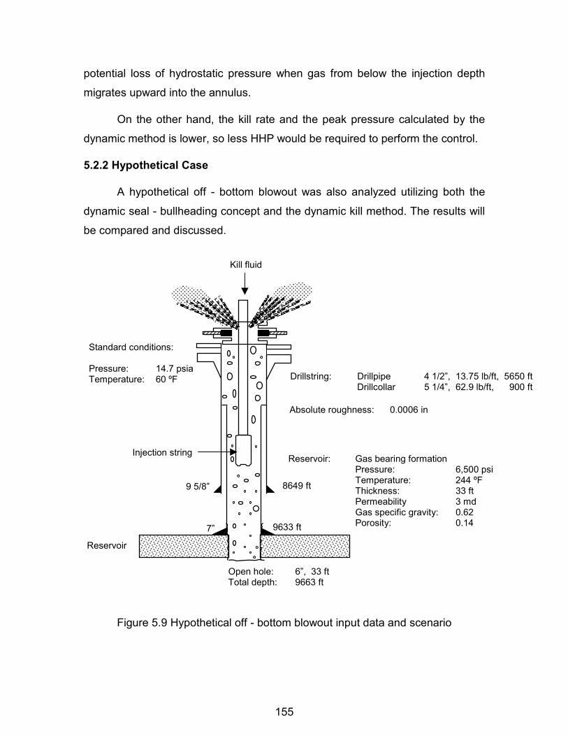
155
potential loss of hydrostatic pressure when gas from below the injection depth
migrates upward into the annulus.
On the other hand, the kill rate and the peak pressure calculated by the
dynamic method is lower, so less HHP would be required to perform the control. 5.2.2 Hypothetical Case
A hypothetical off - bottom blowout was also analyzed utilizing both the
dynamic seal - bullheading concept and the dynamic kill method. The results will
be compared and discussed.
Figure 5.9 Hypothetical off - bottom blowout input data and scenario
9 5/8” 8649 ft
7” 9633 ft
Drillstring: Drillpipe 4 1/2”, 13.75 lb/ft, 5650 ft Drillcollar 5 1/4”, 62.9 lb/ft, 900 ft
Open hole: 6”, 33 ft Total depth: 9663 ft
Absolute roughness: 0.0006 in
Reservoir: Gas bearing formation Pressure: 6,500 psi Temperature: 244 ºF Thickness: 33 ft Permeability 3 md Gas specific gravity: 0.62 Porosity: 0.14
Standard conditions: Pressure: 14.7 psia Temperature: 60 ºF
Reservoir
Injection string
Kill fluid

156
The conditions for the hypothetical blowout were taken from a real well
configuration and reservoir. Figure 5.9 shows the input data and the off - bottom
blowout scenario that was considered for the analysis. The control was calculated considering that the kill fluid was pumped
through the injection string. The computer program can also perform the
calculations for control fluid that pumped through the annular section if the
blowout occurs up the drillstring. In this example, the formation fluid path is from
the bottom of the hole until reaches the injection string. Then, the formation gas
flows to the atmosphere through the annular section between the drillstring and
casings. 5.2.2.1 Dynamic Seal - Bullheading Kill
The proposed method considers use of only one density kill fluid, and it
should be enough to maintain the reservoir pressure in static conditions.
Therefore, the selected kill fluid was a 15 ppg (112-lbm/ft3) brine, which will
generate an overbalance of about 1,000 psi in static conditions. This overbalance
is considered due to the well conditions and seriousness of the circumstances
since it is not possible to shut the well in just after the blowout is controlled but
until the well is secure with the installation or fixing of the surface equipment. The kill parameters and predictions given by the proposed method follow. Kill parameters
The suggested kill parameters for the proposed method are presented in
the Table 5.6. The recommended kill density to control the off - bottom blowout
is 15 ppg (112-lbm/ft3), which is adequate to support the formation pressure in
static conditions. Once the kill density is defined, the kill rate is found by
performing several simulations until obtaining one that fulfills both models,
dynamic seal and bullheading, defined in Chapter 4.

157
Table 5.6 Suggested kill parameters by the proposed method
Kill parameters given by the proposed method
Kill flow rate 14 bpm
Kill fluid density 15 ppg (112 lbm/ft3)
Kill time 1,900 seconds (32 min)
Kill volume 448 bbl
Maximum peak pressure 5,300 psi
Maximum HHP 1,818
The recommended kill rate to generate the dynamic seal and displace the
formation gas into the formation is about 14 bpm. The time to control the off -
bottom blowout utilizing these kill conditions is about 1,900 seconds (32
minutes). Gas flow rate determination
The program utilizes the reservoir and wellbore models previously
presented to obtain the amount of gas flowing under blowout conditions. Figure 5.10 displays the gas flow rate determination after the well has
unloaded all of the liquid and the free flowing equilibrium conditions have been
reached in the system. It plots the bottomhole flowing pressure versus gas flow
rate. The solid line stands for the reservoir inflow performance (IPR) and the
dashed line represents the wellbore hydraulics performance (WHP).
The intersection of these two lines is the simultaneous solution of the IPR
and WHP mathematical models and represents natural flow point of the system
for the given well conditions. It also determines the bottomhole flowing pressure
and blowout gas flow rate, which are about 15,400 Mscfd and 980 psi
respectively.

158
Figure 5.10 Gas flow rate determination of the hypothetical off - bottom blowout
Bottomhole pressure
The program also computes the profile of bottomhole pressure as function
of time during the whole control process. This plot is shown in Figure 5.11. It can
be seen that after the control begins, the pressure increases due to the friction
and hydrostatic pressure of the kill fluid in the annular section. Then, the
injection pressure is reached and the formation gas is forced into the formation
by the kill fluid, generating an additional increase of the bottom pressure due to
the gas compression and due to fact that the lower part of the well is being filled
up with the kill mud.
Bottomhole Flowing Pressure vs Gas Flow Rate
0
1,000
2,000
3,000
4,000
5,000
6,000
7,000
8,000
0 5,000 10,000 15,000 20,000Gas Flow Rate (Mscf/D)
Botto
mho
le F
low
ing
Pres
sure
(psi
)
IPR WHP

159
Figure 5.11 Bottomhole pressure during the control process of the hypothetical off - bottom blowout
Surface pressure
The model also computes the profile of surface pressure as function of
time during the whole control process. This plot is shown in Figure 5.12. The
initial surface pressure is given by the static gas in the drill string, which is
function of the wellbore hydraulic performance in the well when only formation
gas is flowing. After the pumping operations begin the surface pressure
increases due to the friction losses of the kill mud in both the injection string and
annular section. Then, the injection pressure is reached and the formation gas is
Bottomhole Pressure vs Time
0
2,000
4,000
6,000
8,000
10,000
Time (Seconds)
Botto
mho
le P
ress
ure
(Psi
)
Bottomhole Pressure
430 577 724 871 1,018 1,165 1,312 1,459 1,606 1,753 1,900
Kill fluid reaches formation
Kill fluid filling the annulus
Dynamic seal is achieved and bullheading begins
Kill fluid filling the lower zone and displacing gas into the formation
Formation pressure

160
forced into the formation by the kill fluid generating an additional increment of the
surface pressure due to the gas compression. After that the pressure starts to
decrease because of the hydrostatic column generated below of the injection
string helps to overcome the formation pressure. The surface pressure prediction
is a very important parameter since it can assist in the selection of the
appropriate pumping system and in monitoring whether the actual job is
proceeding as expected. Hence, a better kill job may be performed.
Figure 5.12 Surface drillpipe pressure during the control process of the hypothetical off - bottom blowout
Surface Pressure vs Time
0
1,000
2,000
3,000
4,000
5,000
6,000
7,000
8,000
Time (Seconds)
Surfa
ce P
ress
ure
(Psi
)
Surface Pressure
430 577 724 871 1,018 1,165 1,312 1,459 1,606 1,753 1,900
Kill fluid filling the annulus
Dynamic seal is achieved and bullheading begins
Kill fluid filling the lower zone and displacing gas into the formation
Kill fluid reaches formation

161
Gas flow rate during the control operation
The gas flow rate during the control operation as function of time is
another output of the program. This behavior is presented in Figure 5.13. It can
be seen that the gas flow rate before to start the pumping operation is about
15,400 Mscfd. After the control operations commence the gas flow rate
decreases due to the increasing of the bottomhole pressure caused by the kill
fluid flowing in the annular section. Then, the injection pressure is reached and
the gas is displaced by the kill fluid into the formation (bullheading process). The
increase in the gas rate flowing into the formation is due to the increase in
hydrostatic pressure caused by the control fluid.
Figure 5.13 Gas flow rate during the control process of the hypothetical off - bottom blowout
Gas Flow Rate vs Time
-15,000
-10,000
-5,000
0
5,000
10,000
15,000
20,000
Time (Seconds)
Gas
Flo
w R
ate
(Msc
f/d)
Gas Flow Rate
430 577 724 871 1,018 1,165 1,312 1,459 1,606 1,753 1,900

162
Tables as example of the outputs of the program presenting the
bottomhole pressure, surface pressure and gas flow rate as well as the
conditions during the bullheading process as function of time for the hypothetical
blowout are presented in Appendix C. 5.2.2.2 Conventional Off - Bottom Dynamic Kill
The computer program also contains the dynamic kill model. Therefore, a
comparison of the two methods can be made for the same off - bottom blowout
with identical wellbore geometry, reservoir properties and type of kill fluid. The
dynamic kill method analysis is based on the steady state system analysis
approach as presented in Figure 5.14. It shows that if a rate of 5 bpm is pumped
the wellbore hydraulics performance curve intersects the reservoir inflow
performance curve which means that a stable flow condition results and the
reservoir continues producing at a gas flow rate of about 11,500 Mscfd. However
if the kill rate is increased to about 9 bpm, the wellbore hydraulics performance
curve is practically tangent to and just above the inflow performance curve. This
means that at that rate a stable gas lift flow condition would not be possible, and
the well would be killed. Thus the minimum kill rate for a conventional dynamic
kill is 9 bpm.
The suggested kill parameters for the dynamic kill method are presented
in Table 5.7. Since the analysis was performed with the same kill fluid type to
make a meaningful comparison, the two methods propose the same kill density
and viscosity, which are 15 ppg (112-lbm/ft3) and 20 cp. The recommended kill
rate by the dynamic method is about 9 bpm.
Table 5.7 Suggested kill parameters by the dynamic method
Kill parameters given by the dynamic kill method
Kill flow rate 8.8 bpm
Kill fluid density 15 ppg (112 lbm/ft3)
Maximum peak pressure 4,697 psi
Maximum HHP 1,102

163
Figure 5.14 Dynamic kill analysis of the hypothetical off - bottom blowout
Table as example of the outputs of the program presenting the
conventional dynamic kill results for only gas flow rate for the hypothetical
blowout is presented in Appendix C. 5.2.2.3 Comparison of the Predicted Results
The relative advantages of dynamic seal – bullheading and conventional
dynamic kill methods can be assessed by comparing the results of the kill
parameters and predictions for applying these two methods to the two examples
in this chapter. The potential advantages of the dynamic seal - bullheading
method are that it requires less mud volume, less time, and lower mud weight,
Bottomhole Flowing Pressure vs Gas Flow Rate
0
1,000
2,000
3,000
4,000
5,000
6,000
7,000
8,000
0 5,000 10,000 15,000 20,000
Gas Flow Rate (Mscf/D)
Botto
mho
le F
low
ing
Pres
sure
(psi
)
IPR WHP
8.8 bpm
0 bpm
5.0 bpm

164
and provides a more positive kill. The potential advantages of a conventional
dynamic kill are that it requires less pump horsepower, less pump rate capacity,
and lower surface pressures, and it imposes less pressure on surface and
downhole equipment and on potential lost circulation zones.
Examples of these are evident when Table 5.4 is compared with Table 5.2
and Table 5.5, and 5.6 is compared with Table 5.7. As expected, the proposed
method requires a higher kill rate since it has to deliver both upward and
downward flow rates during the control. The upward rate must maintain the
dynamic seal through the annular section between the injection string and the
casings, and the downward rate must displace the formation gas into the
producing zone. For the actual field case, the required rate for the proposed
method was 18.8 bpm versus a minimum of 15 bpm calculated for a conventional
dynamic kill. The maximum pump pressure required for the proposed method
was 6,961 psi compared to 6,010 psi for the conventional method. The rates and
pressure are close for both methods, apparently because pressures in this
example are hydrostatic dominated.
The results for the hypothetical case are quite different. The required rate
and maximum surface pressure for the proposed method are 14 bpm and 5,300
psi respectively. These are both larger than the 8.8 bpm and 4,697 psi required
for a conventional kill. The maximum bottom hole pressure predicted for the
proposed method is almost 8,400 psi versus 7,600 psi for conventional control.
Therefore, the proposed method potentially provides a much more rapid
kill, but may also require significantly more pump capacity and pressure and
poses more risk of pressure related failures both downhole and at the surface. 5.3 Advantages and Disadvantages of the Proposed Method
The overall advantage of the dynamic seal - bullheading procedure
compared with the conventional dynamic kill is that the proposed method should
provide a more reliable and conclusive off - bottom kill because the formation
fluids will be forced back into the formation and the well completely filled with a

165
kill density fluid. Generally, this means that the well can also be controlled more
quickly with a minimal control fluid volume because the method ensures efficient
displacement of the blowout fluids into open hole formations. It also should
eliminate or minimize the need for further well control operations after the kill is
completed.
The dynamic method, on the other hand, does not guarantee that the
formation fluid is displaced from the wellbore. It is uncertain whether, and how
much, gas remains in the well. Once pumping ceases, any remaining gas will
migrate and will tend to unload the well again unless some additional control
actions are taken. Possible examples are re-establishing a surface shut in and
instituting volumetric control methods, and tripping in the hole in order to circulate
out the remaining gas either using conventional well control methods or by
circulating at a rate that keeps bottomhole pressure greater than formation
pressure.
The proposed method should also provide more reliable kill parameters,
because it considers known fluid properties from the surface to the bottom of the
well whereas the real conditions below the injection depth are uncertain during
conventional dynamic kills.
One example is that the proposed method should define a lower, but more
reliable kill density. This results from the proposed method completely filling the
well with the control fluid, whereas the conventional dynamic kill can only insure
that the length from the injection depth to the surface contains the control fluid.
This can require very high kill fluid densities to ensure hydrostatic control. In the
hypothetical case, a 15 ppg mud provides an off – bottom dynamic kill at a pump
rate of 8.8 bpm. However, a 19.1 ppg mud would be required to ensure
hydrostatic control. Under some circumstances, the required density would be
impossible to achieve.
Another example is that the required kill volume with the proposed method
is defined, whereas the volume that must be pumped to insure a complete kill
with the conventional method is uncertain because fluid behavior below the

166
injection point is uncertain. Therefore, even the sophisticated, commercial, time-
based simulators cannot presently give rigorous predictions for off – bottom
conditions.
The proposed method involves controlling the well with one fluid density
and avoids additional operations to change the control fluid density as is
sometimes performed with the conventional dynamic kill. This simplifies both
planning and operations, but overrides the possibility of minimizing the surface
and subsurface pressures required for control by using low density fluids as
envisioned by Blount32.
A related disadvantage of the proposed method is that the higher rates
impose higher pressures on surface and downhole equipment and on the open
formations. Therefore, the equipment used must have higher pressure ratings
and the risk of lost returns, and possibly of an underground blowout, is increased. The primary advantage of the conventional dynamic kill is that it requires
lower rate and therefore, involves lower pressures. A relatively new concept for
defining a truly minimum kill rate for off – bottom kills has been described by
Flores-Avila et al63. These methods have increased potential to be practical for
early implementation using existing rig equipment because the rate and pressure
capabilities required are lower than those required by the proposed method.
The preferable method for a specific situation is obviously dependent on
the well conditions, equipment capability and availability, and other factors. The
methods described herein are intended to provide a quantitative basis for
selecting between the dynamic kill and dynamic sea - bullheading methods for
any specific situation.

167
CHAPTER 6
SUMMARY, CONCLUSIONS AND RECOMMENDATIONS
A study of the two current, off – bottom, blowout control engineering
procedures used in the oil and gas industry has been performed. This research
also proposes an alternative engineering design procedure to control off - bottom
blowouts. An off - bottom blowout is any blowout where there is not an intact flow
path to allow fluids to be injected from the surface to the bottom of the well. The
following summary and conclusions were drawn from this investigation.
Recommendations are also made for improving the proposed new method. 6.1 Summary
The dynamic and momentum kill are the only currently available methods
in the petroleum industry to control off - bottom blowouts by pumping kill fluid
through an injection string into the well. In this research, a comprehensive study
of these two current engineering concepts was performed, and a thorough review
of published historical and hypothetical cases applying these techniques was
accomplished. A computer program for each method was built to assist in this
analysis. The advantages, important shortcomings, and design problems of each
method were identified by this study.
An alternative engineering design procedure to control off - bottom
blowouts was also developed. This method is called "dynamic seal -
bullheading". It is essentially a combination of the dynamic kill and bullheading
concepts. The principle of this method is based on two important stages. First a
dynamic seal has to be generated at the injection string depth. And second, a
portion of the kill fluid is forced to flow downward below the injection pipe to
displace the remaining formation fluid in the wellbore to go back into an open
formation. In other words, the procedure is based on achieving a pressure
distribution in the system that uses a high pressure gradient from the string depth

168
to the surface due to the kill flow rate and density to force the well fluids to
simultaneously move downward to be injected in an open formation.
A model of this concept was defined and implemented in a computer
program that can predict the effect of potential kill parameters such as kill flow
rate, kill fluid density, kill fluid volume, pumping time, and effect of control depth.
It predicts the formation fluid influx, surface pressure, bottomhole pressure, and
pressure at critical points in the well as a function of time for a job using the
selected parameters.
The new computer program was utilized on two different off - bottom
blowout scenarios to simulate and analyze the control of each. The first is an
actual field case and the second is a hypothetical blowout with input data from a
real well configuration and reservoir. The same blowouts were also analyzed
utilizing the conventional dynamic kill. The results were compared and discussed.
The computer program developed in this work can be utilized to analyze
the following surface and underground blowout control processes: �� Off - bottom dynamic seal - bullheading kill
�� On and off - bottom dynamic kill
�� Relief well dynamic kill
�� Bullheading operations
A bullheading mathematical model was required to predict behavior of the
well during the bullheading phase of the proposed method. Therefore, a
bullheading model was developed in this work to compute the required kill
parameters such as kill flow rate, kill density, and kill volume. The model also
calculates the surface pressure, interface (kill fluid - formation fluid) pressure and
position, and bottom hole pressure as a function of time during the bullheading
process.

169
6.2 Conclusions 6.2.1 Conventional Dynamic Kill Method
The conventional dynamic kill method has been well defined in the
literature and widely applied to surface and underground blowouts. The following
conclusions have been reached by this study. 1. The conventional dynamic kill method, which is based on the steady state
system analysis approach, has been utilized in several off - bottom blowout
control operations and is currently the only proven method for these
situations. 2. The steady state systems analysis approach was shown to be applicable to
all of the field cases analyzed in this study. Consequently, this is a proven
method for designing and analyzing off – bottom kills. 3. The kill rates, and consequently the pressures, required for a conventional
dynamic kill are lower than for the proposed method. This can be an
advantage if there are equipment or subsurface pressure limitations. 4. Some limitations and shortcomings occur when this method is applied to off –
bottom conditions, i.e. where the injection string is distant from the bottom of
the well. Specifically, the method does not take into account that the kill fluid
may fill the wellbore from the injection point to the bottom of the well, and
assumes that only formation fluid remains in the part of the wellbore during
the control. This assumption requires that the mud density from the injection
depth to the surface be sufficient to balance the formation pressure in static
conditions with the following consequences. 5. The calculated density may be higher than can practically be achieved. In this
case, the opportunity for in-well control would be discarded, and another more
expensive or time consuming blowout control methodology such as snubbing
in or drilling a relief well would be adopted, potentially unnecessarily.

170
6. A considerable amount of gas may remain in the section below the injection
point. If the circulation rate is reduced or stopped, the gas may start to
migrate, expanding, and causing the well to begin to unload again. This
possibility typically requires additional procedural steps after achieving an
initial dynamic kill. 7. The steady state systems analysis approach cannot precisely determine the
optimum kill parameters because of the uncertainty about the real conditions
and mixture properties below the injection depth. A specific example is that
the total volume of mud required cannot be precisely defined. 6.2.2 Momentum Kill Method
The momentum kill has been described as a method for controlling off -
bottom blowouts. Based on both the logical analysis of the concept and specific
example calculations for actual kills, it is concluded that the momentum kill
design method is irrelevant for controlling blowouts. The field results attributed to
momentum kills in published reports can be explained by analyzing these cases
as dynamic kills. 6.2.3 Dynamic Seal - Bullheading Kill Method
An alternative concept for off – bottom well control, the dynamic seal –
bullheading method, has been defined. It uses a dynamic kill - like procedure to
impose a wellbore pressure that is high enough to displace formation fluids into
open formations in the well. The following conclusions about this new alternative,
developed by combining previous methods, have been reached. 1. The overall advantage of the dynamic seal – bullheading procedure is that it
should provide a more reliable and conclusive off – bottom kill because the
formation fluids are displaced from the well and replaced with a kill density
fluid. Therefore, the risk that any gas will remain below the injection point,
which would migrate and tend to unload the well, is minimized.

171
2. The higher rates used and positive displacement achieved should result in
minimum job times and volumes pumped. 3. Both planning and operations are simplified by use only one density fluid
completely filling the well. However, this overrides the possibility of minimizing
surface and subsurface pressures required for control by using low density
fluids as envisioned by Blount32. 4. The dynamic seal – bullheading computer program can assist in off - bottom
blowout control analysis and design. The many parameters that affect off -
bottom blowout control design and the kill process can be investigated. These
analyses can consider the effects of different kill fluid rate, density and
viscosity, and injection string geometry and depth by changing the input data.
This capability can be used to help determine the most appropriate kill
approach for a given set of conditions, including the potential of achieving a
kill with existing rig equipment. 5. The computer program was utilized to simulate the hydraulic conditions
during the control of an actual underground blowout70 for the different pump
rates and kill fluid densities utilized. The pressures predicted by the program
have reasonably good agreement with the ones measured during the control.
In addition, the individual dynamic seal and bullheading model predictions
were also good when compared to published field case histories. 6. Likely applications for this method are similar to those for bullheading in
general, but utilize the dynamic seal rather than a surface shut in.
Nevertheless, the casing and/or formation strengths above the producing
formation must be high enough to contain the pressure required to force the
column of formation fluids back into an open formation, ideally the producing
formation. If formation fluids are forced into fracture at a pressure that is
inadequate to also force these fluids into the producing formation, an
underground blowout may result.
172
7. A disadvantage of the proposed method is that the higher rates impose higher
pressures on surface and downhole equipment and on the open formations.
Therefore, the equipment used must have higher pressure ratings and the
risk of lost returns, and possibly of underground blowout, is increased and
must be considered explicitly. 8. When a blowout takes place, the magnitude of the blowout consequences
can depend on the time to regain the control of the well. The selection of the
intervention technique becomes a critical decision. Therefore, the optimum
approach should be identified and implemented rapidly to lead to a successful
blowout control operation on the first attempt and in the minimum amount of
time. 6.3 Recommendations
The following recommendations are made for improving and validating the
proposed new method. 1. Full-scale experiments to simulate the dynamic seal - bullheading process
should be performed to demonstrate this method and help validate the
models. This can be accomplished using the LSU#1 research well with some
variation in well conditions and kill parameters. 2. Additional research needs to be carried out about the mathematical behavior
of simultaneous upward and downward liquid flow since this is practically a
new concept in blowout control and there is not a rigorous mathematical
model to predict this phenomenon. It might be accomplished by performing a
meticulous simultaneous solution among the injection string, annular section
and the bullheading model, taking the injection depth as the solution point.
The simultaneous upward and downward liquid flow is present after the
dynamic seal is attained. 3. A fracture model should be added to the computer program to simulate how
the fracture initiation and fracture propagation affects the pressure behavior
during the control.

173
4. The possibility of including more than one permeable formation within the
wellbore should be investigated as an improvement to the program. The
same reservoir model can be utilized with different rock and formation fluid
properties appropriate to each formation. 5. The dynamic seal model was applied to give a series of steady state solutions
to involve the time in the process and obtain the required volume to reach the
dynamic seal, however a more rigorous time – based simulation method such
as a conventional finite difference approximation is recommended to model
the dynamic seal process. 6. Experiments in the LSU’s 48-ft flow loop at different deviation angles should
be conducted to establish a good basis for the development of a model of
minimum velocity for effective bullheading for application to directional and
high angle wells. 7. The mathematical models in the computer program should then be adapted to
apply the proposed method in directional high angle well.

174
REFERENCES
1. Bourgoyne A.T. Jr., Millheim K., Chenevert M,, Young F., Applied Drilling Engineering, Society of Petroleum Engineering, Richardson Texas, 1991.
2. Grace, Robert D., Advanced Blowout & Well Control, Gulf Publishing
Company, Houston, TX, 1994. 3. Syllabus "PETE 4060 - Prevention of Oil and Gas well Blowouts" The Craft
and Hawkins Department of Petroleum Engineering. Louisiana State University. Baton Rouge, LA 2000.
4. Skalle P., Jinjun H. and Podio A.L., "Killing Methods and Consequences of
1120 Gulf Coast Blowouts During 1960-1990" SPE 53974 presented at the SPE Latin American and Caribbean Conference, Caracas Venezuela. April 1999.
5. Holand P., Offshore Blowouts: Causes and Control, Gulf Publication Co.
Houston, Texas, 1997. 6. Grace, Robert D., "Practical Considerations in Pressure Control Procedures
in Field Drilling Operations", Journal of Petroleum Technology. August 1977. 7. Watson W. David and Moore Preston L., "Momentum kill procedure can
quickly control blowouts", Oil & Gas Journal, August 30, 1993. 8. Grace, Robert D., "Fluid dynamics kill Wyoming icicle" World Oil, April 1987 9. Grace, Robert D. and Bob Cudd, "Fluid dynamics used to kill South Louisiana
blowout", World Oil, April 1989. 10. Hansen, Arthur G., Fluid Mechanics New York, John Wiley and Sons, Inc.
1967. 11. Roberson, John A. and Crowe, Clayton Engineering Fluid Mechanics 2nd
edition, Houghton Mifflin Company. 1980. 12. Zucrow, Maurice J. and Hoffman, Joe D., Gas Dynamics Volume 1, New York
John Wiley and Sons, Inc. 1976. 13. Olson, Ruben M., Essentials of Engineering Fluid Mechanics 4th edition, New
York Harper & Row Publishers, 1980.

175
14. Mott, Robert L., Applied Fluid Mechanics 5th edition, Prentice Hall New Jersey. 2000.
15. Noel de Nevers, Fluid Mechanical For Chemical Engineers 2nd edition, New
York McGraw Hill, Inc. 1991. 16. Massey B. S., Mechanics of Fluids" 4th edition, London Van Nostrand
Reinhold Company. 1979. 17. Gordon J. Van Wylen and Richard E. Sonntag ,Fundamentals of Classical
thermodynamics, 3rd edition, New York John Wiley and Sons, Inc. 1986. 18. Blevins, Robert D., Applied Fluid Dynamics Handbook, New York, London
Van Nostrand Reinhold Company. 1984. 19. Fox, Robert W. and McDonald, Alan T., Introduction to Fluid Mechanics
,Fourth Edition John Wiley & Sons, Inc. 1992. 20. Craft B. C. and Hawkins M. F., Applied Petroleum Reservoir Engineering, 2nd
edition, Prentice Hall 1991. 21. Smith R. V. Practical Natural Gas Engineering, 2nd edition, Tulsa, Oklahoma.
Pennwell Books. 1990. 22. Beggs H. Dale, Gas Production Operations, Oil and Gas Consultants
international publications, Tulsa, Oklahoma. 1984. 23. Syllabus "PETE 7201 - Flow in Porous Media" The Craft and Hawkins
Department of Petroleum Engineering. Louisiana State University. Baton Rouge, LA 1999.
24. Syllabus "PETE 7202 - Advanced Well Testing" The Craft and Hawkins
Department of Petroleum Engineering. Louisiana State University. Baton Rouge, LA 1999
25. Jardine S.I., Johnson A.B., With D.B. and William Stibss, "Hard or Soft Shut-
In: Which is the Best Approach?”, SPE/IADC 25712, presented at the SPE/IADC Drilling Conference, Amsterdam, 1993.
26. Syllabus "PETE 4060 – Well Design Production", The Craft and Hawkins
Department of Petroleum Engineering. Louisiana State University. Baton Rouge, LA 1999.
27. William, Abel L. "Kill operations requires thorough analysis", Oil & Gas
Journal, May 15, 1995.

176
28. Wessel, Michael and Tarr, Brian A., "Underground Flow Well Control: The Key to Drilling Low-Kick-Tolerance Wells Safely and Economically", SPE 22217, December 1991.
29. Wessel, Michael and Tarr, Brian A., "Underground Flow Well Control: The
Key to Drilling Low-Kick-Tolerance Wells Safely and Economically", SPE 23764, Supplement to SPE 22217.
30. Grace, Robert D. and Burton M.R., "Mud Lubrication - A viable Alternative in
Well Control", SPE/IADC 35212 presented at the SPE/IADC Drilling Conference, New Orleans, Louisiana, 1996.
31. Oudeman Pieter, Baaijens M.N., Mij B. V. and Dick Ter Avest, "Modeling
Blowout Control by Means of Downhole Kill Fluid Injection", SPE 26732 presented at the SPE Offshore European Conference, Aberdeen, 1993.
32. Blount E.M. and Soeiinah E., "Dynamic Kill: Controlling Wild Wells a New
Way", World Oil, October 1981. 33. Kouba G.E., MacDougall G.R. and Schumacher B.W., "Advanced in Dynamic
Kill Calculations for Blowout Wells" SPE 22559 presented at the SPE Drilling & Completion Conference, September 1993.
34. Brill, James P. and Mukherjee, Hemanta, Multiphase Flow in Wells, SPE
Monograph Volume 17. 35. Koederitz, W.L., "Gas Kick Behavior During Bullheading Operations in
Vertical Wells", Ph.D. Dissertation, Louisiana State University, Baton Rouge, LA, 1995.
36. William, Abel, et al, Firefighting and Blowout Control, Wild Well Control, Inc,
Spring, TX. 1994. 37. Adams, Neal and Kuhlman, Larry Kicks and Blowout Control, Second Edition
Pennwell Publishing Company, Tulsa, Oklahoma, 1994. 38. Kreyszig Erwin Advanced Engineering Mathematics, 8th Edition John Wiley
and Sons, Inc. 1999. 39. White Frank Fluid Mechanics, Second Edition McGraw-Hill, Inc 1986. 40. Anderson D. Tannehill J. and Pletcher R. Computational Fluid Mechanics and
Heat Transfer, Hemisphere Publishing Corporation. 1984 41. Anderson J. Jr. Computational Fluid Dynamics, McGraw-Hill, Inc 1995.

177
42. Nickens H. V. "A Dynamic Computer Model of a Kicking Well" SPE 14183. Presented at the 60th Annual Tech. Conf. Las Vegas, NV. 1985
43. Starrett P. and Sepehrnoori K. "A shallow Gas Kick Simulator Including
Diverter Performance" SPE 18019, 1990. 44. Jun F., Tai-He S., and Zhang-Gui L., "A Dynamic Model and Simulation for
Killing of Empty Hole Blowout", SPE 49963 presented at the Asia Pacific Oil and Gas Conference and Exhibition held in Pert Australia, October 1998.
45. Gregory G. and Fogarasi M. ,"Alternate to Standard Friction Factor Equation"
, Oil and Gas Journal, April 1 1985. 46. Oudeman, P., "Kill Procedures to Avoid Formation Damage in the High Rate
Gas Wells of an Underground Storage Project", SPE 54761 presented at the SPE European formation Damage Conference, The Hague Netherlands. May 1999.
47. Taitel, Y., Barnea, D., "Counter-Current Gas-Liquid Vertical Flow, Model for
Flow Pattern and Pressure Drop", International journal of multiphase flow, Vol. 9, No. 6: 637-647. 1993.
48. Bourgoyne A.T. Jr., Wang Y., Bourgoyne D.A., "Experimental Study of Liquid
Holdup During Well Unloading and During an Off-bottom Dynamic Kill”, LSU/MMS Well Control Workshop. March 30-31, 1994.
49. SPE Reprint Series No 42 "Well Control" 1996. 50. Lynch R. D., McBride E., Perkins T., Wiley M., "Dynamic Kill of an
Uncontrolled CO2 Well" SPE 11378, July 1985. 51. Koederitz W. L., Beck F.E., Langlinais J.P. and Bourgoyne A. T. Jr., "Method
for Determining the Feasibility of dynamic Kill of Shallow Gas Flows", SPE 16691 presented at the Annual Technical conference and Exhibition, Dallas Texas, September 1987.
52. Gillespie John D., Morgan Richard F., and Perkins Thomas K., "Study of the
Potential for an Off - Bottom Dynamic Kill of a Gas Well Having and Underground Blowout", SPE 17254 presented at the 1988 IADC/SPE Drilling Conference. Dallas Texas, 1988.
53. Al-Shehri Dhafer A., "A Study in the Dynamic Kill for the Control of Induced
Surface Blowouts", Ph.D. Dissertation, Texas A & M University, 1994.

178
54. Oudeman P., and Mason D., "Results of a Field Test to Improve Hydraulic Blowout Control Calculations", SPE 50577 presented at the European Petroleum Conference held in The Hague, The Netherlands. October 1998.
55. Osornio C., Castro H., Vallejo V., and Ayala E., "Successful Well Control in
the Cantarell Field Applying the Dynamic Method", SPE 71372 presented at the Annual Technical Conference and Exhibition held in New Orleans, Louisiana. September - October 2001.
56. Ikoku, Chi U. Natural Gas Engineering, Penn well Publishing Co. Tulsa
(1980). 57. Santos Otto L., "A dynamic Model of Diverter Operations for Handling Shallow
Gas Hazards in Oil and Gas exploratory Drilling", Ph.D. Dissertation, Louisiana State University, Baton Rouge, LA (1989).
58. Bourgoyne Adam T. Jr., Barnett David, and Eby Dan, "New Developments in
Computer Modeling of Blowout Control Operations", IADC Well Control Conference of The Americas held in Rio de Janeiro, Brazil. July - August 1996.
59. Santos Otto L., "A Study on Blowouts in Ultra Deep Waters", SPE 69530
presented at the Latin American and Caribbean Petroleum Engineering Conference held in Buenos Aires Argentina, March 2001.
60. Beggs H. Dale, Production Optimization Using NODAL Analysis, Oil and Gas
Consultants international publications, Tulsa, Oklahoma. 1991. 61. Turner, R.G., Hubbard, M.G., and Duckler, A.E., "Analysis and Prediction of
Minimum Flow Rate for the Continuous Removal of Liquid from Gas wells", JPT (November 1969) 21, 1475 - 1482.
62. Bourgoyne, A.T., Wang Y., Bourgoyne, D.A., "Experimental Study of Liquid
Holdup during Well Unloading and During an Off - Bottom Dynamic Kill", LSU/MMS Well Control Workshop (March 1994) Baton Rouge Louisiana.
63. Flores-Avila F., Smith J. R., Bourgoyne A.T., Bourgoyne, D. A., "Experimental
Evaluation of Control Fluid Fallback During Off - Bottom well Control: Effect of deviation angle", IADC/SPE 74568 prepared for presentation held in Dallas Texas, February 2002.
64. Lee J., Wattenbarger R., Gas Reservoir Engineering, SPE Textbook Series
Vol. 5 Richardson TX. 1996.

179
65. Wattenbarger R. A., Ramey H. J. Jr., "Gas Well Testing With Turbulence, Damage and Wellbore Storage", J Pet Tech (Aug 1968) 877 - 887 Trans, AIME, 243.
66. Langlinais J. P., Bourgoyne A. T. Jr., Holden W. R., "Frictional Pressure
Losses for the Flow Drilling Mud and Mud/Gas Mixtures", SPE 11993 presented at the SPE Annual Technical Conference and Exhibition, San Francisco, CA. October 1983.
67. Elfaghi F. A., Langlinais J. P., Bourgoyne A. T. Jr., Holden W. R., "Frictional
Pressure Losses for Single Phase and Two Phase Flow of Drilling Muds", Journal of Energy resources Technology. Vol. 105 - 372 September 1983.
68. McCain William D. Jr., The Properties of Petroleum Fluids, Second edition
Pennwell Publishing Company. Tulsa, Oklahoma. 1990. 69. Dake L. P., Fundamentals of Reservoir Engineering, Elsevier Publishing
Company 1978. 70. Smith J. R., Bourgoyne, A. T. Jr., Waly, S. M., and Hoff, E. B., "Case
Histories Bring Reality to Well Control Training", IADC Well Control Conference of the Americas. August 25-26, 1999.

180
APPENDIX A
DERIVATION OF THE MOMENTUM KILL EQUATIONS
The mathematical model of Momentum kill is based on the Newton's
second Law of Motion16. Hence, the control volume formulation of Newton's
second law, also know as the linear momentum equation is given by:
� � ���
�� dAvvdVvt
M �� (A-1)
Considering that the equilibrium condition has been reached after the well
has been completely unloaded of all the mud and only formation fluid is flowing,
the above equation becomes:
� �� dAvvM � (A-2)
Developing the analysis for small intervals, a constant area for each
interval can be considered. Therefore, Equation A-2 can be written as:
vAvM �� (A-3)
In order to use English Engineering system of units, a constant of
proportionality ( cg ) must be included for the equation to be dimensionally
homogeneous.
cgvAvM �
� (A-4)

181
Substituting vAq � in the Eq. A-4
cgqvM �
� (A-5)
On the other hand, the Mass conservation law, which states that the rate
of increase of mass within the control volume plus the net rate at which mass
flows out of the control volume is equal to zero, and is mathematically
represented by:
� � ���
�� dAvdVt
��0 (A-6)
Again considering that the equilibrium condition has been reached when
only formation fluid is flowing, Eq. A-6 becomes:
� �� dAv�0 (A-7)
Contemplating small length and constant area intervals, the above
Equation would be:
0 vA�� (A-8)
Equation A-8 can be also written as:
AvvA nn�� � (A-9)
Solving the previous equation for velocity at the n interval.

182
Aq
AvAv
nnn
�
�
�
��� (A-10)
The gas density at the n interval can be computed utilizing the real gas
law, which is given by:
nn
ngn RTz
pM�� (A-11)
Where: agg MM ��
Substituting the molecular weight of the gas ( gM ) in Eq. A-11
nn
nagn RTz
pM�� � (A-12)
Substituting Eq. A-12 in Eq. A-10
ApM
RTqz
ARTzpMqv
nag
nn
nn
nagn
�
�
�
��
���
����
�� (A-13)
Equation A-13 gives the formation fluid velocity at n conditions, and is the
required one to calculate the momentum of the fluid given by Eq. A-5. Therefore,
substituting Eq. A-13 in Eq. A-5.
c
nag
nn
g
qApM
RTqz
M
��
�
��
�
�
��
�
�
� (A-14)

183
Simplifying the above equation
cnag
nngscgscg AgpM
RTzqM
�
�22
� (A-15)
Considering the following constant values: RlbmftpsiaR
�
�
�
�
3
73.10
966.28�aM
2sec2.32
�
�
�
lbfftlbmgc
ApTzq
Mng
nngscgscg
�
�22
0115.0� (A-16)
Equation A-16 gives the momentum of the gas flowing up.
The momentum for the kill fluid is derived as follows. Taking Eq. A-5 and
substituting Aqv /� gives:
cgq
AqM �
� (A-17)
Simplifying the above Equation.
c
Mkfkfkf Ag
qM
2�
� (A-18)
In Equations A-16 and A-18, the area, A , considered is that of the wellbore just
below the injection point. Solving Eq. A-18 for the control fluid flow rate.

184
kf
ckfMkf
AgMq
�� (A-19)
Equation A-19 can be utilized to obtain the kill flow rate of a given fluid
density to reach a required momentum. The required momentum must be at least
that generated by the gas. Therefore, kfM in Eq. A-19 would be substituted by
gM given by Equation A-16

185
APPENDIX B
DERIVATION OF THE PRESSURE GRADIENT EQUATION
The pressure gradient equation is given by a combination of the
Conservation of Momentum and Conservation of Mass. This appendix will show
first the derivation of the conservation of momentum and then will combine the
two conservation principles to obtain the pressure gradient equation.
The principle of Conservation of Momentum is derived from Newton's
second Law of Motion14, which states that the net force acting on a system is
equal to the rate of change of momentum of that system. Only forces acting at
the boundaries of a prescribed space are concerned: any force within the space
is involved only as one half of an "action - and - reaction" pair and so does not
affect the overall behavior. Mathematically, the Newton's second law can be written as:
� �DtMD
DtDvmmaF ���� (B-1)
The forces (F ) acting in the boundary of a control volume that is inside of
a circular pipe with upward flow are shown in Figure B-1.
The flow system is one-dimensional spatial geometry along wellbore and
pipe due to the limited cross sectional size compared with the axial wellbore and
pipe length.

186
A2
V2
FP2= P2A2
V1
A1
FT
FB
P2
FP1= P1A1
P1
L
Figure B-1 Forces acting in the system
Applying the Equation B-1 to a fluid flowing through the control volume
yields the control volume formulation of Newton's second law10,17. It is also
known as the linear momentum equation, which is given by:
����
����
cvcsexternal dVv
tdAvvF �� (B-2)
Where the external forces ( externalF ) are divided in surface forces and body forces.
�����
�����
cvcsBS dVv
tdAvvFF �� (B-3)
Surface forces ( SF ) are those that act on the boundaries of the system by
virtue of their contact with the surroundings. Surface forces may be subdivided

187
into normal forces and tangential forces. Therefore, the above equation
becomes:
������
������
cvcsBTP dVv
tdAvvFFF �� (B-4)
Where:
� �
cs
dAvv� =Flow rate of momentum (momentum flux through the control volume)
��
�
cv
dVvt
� = Rate of change of momentum of the fluid in the control volume.
The components in the Equation B-4 are defined as follows: Normal Force ( PF ): Force due to the pressure into the system. It is given by:
���
csP dApF (B-5)
Where: �p Pressure at the interest depth.
�A Flow area.
The negative sign is introduced because pressure is a compressive stress
acting in the inward direction on a surface and, for the surface element dA the
positive normal acts in the outward direction.

188
Tangential Force ( TF ):
The tangent fluid force is due to the viscous shearing stress of the fluid. It
is given by:
� ��
csT dF � (B-6)
Where: �� Shear stress.
�� Contact area (surface of the pipe to oppose the flow, it can be
through pipe, dL �� or through annulus, edL �� ).
Body Force ( BF ):
The body force is due to the gravity force, which acts in the direction of the
gravitational field. It is given by:
��
cvB dVgF � (B-7)
Where: �g Acceleration of gravity.
�� Fluid density.
�V Volume of fluid over the interest depth.
Flow rate of momentum (momentum flux) ( � �
cs
dAvv� ):
This term represents the flux or transport of momentum across the
boundaries of the control surface.

189
Rate of change of momentum ( ��
�
cv
dVvt
� ):
This term represents the time rate of change of momentum of the fluid
within the control volume. This term applies in unsteady flow conditions.
Substituting the acting forces (Equations B-5, B-6 and B-7) on the surface
control into the Equation B-4.
����� ��
��������
cvcscvcscs
dVvt
dAvvdVgddAp ���� (B-8)
Equation B-8 is the linear momentum equation in an Integral control
volume representation, which is widely used in problems related with fluid
mechanics. Another very common representation of the one-dimensional momentum
equation is in differential form17,10, which all the terms are per unit volume. The
flow rate of momentum (momentum flux) and the rate of change of momentum in
differential form are derived as follows: The second representation of the equation B-1 is given by:
DtDvmF �� (B-9)
The derivative in the above equation is a derivative following a system of a
fluid particle. Consequently, it is the substantial derivative38 (also called material
derivative), and by definition in one dimension it is given by:
tv
Lvv
DtDv
�
��
�
��
)()( (B-10)

190
The first term of the right-hand side is called the convective acceleration,
which arises when the particle moves through regions of varying velocity. The
second one is called the local acceleration, which vanishes if the flow is steady
(independent of time), in other words only an unsteady state can induce the local
acceleration term. Substituting the above equation in the Newton's second law,
and considering the terms per unit volume.
��
���
�
�
��
�
�� t
vLvvF )()(
� (B-11)
Rearranging the previous equation becomes:
tv
LvF
�
��
�
���
)()( 2�� (B-12)
Now the left-hand side components given on Eq. B-8 will also changed to
differential form. The pressure term (normal force) in Eq. B-8 is changed to
differential form using the divergence theorem of Gauss38, which states that
surface integrals can be transformed into volume integrals. It is mathematically
given by:
dVdAVA�� ���� div (B-13)
Where the divergence of the function � is represented by:
zyxzyx
�
���
�
���
�
����div (B-14)
Therefore, applying the divergence theorem.

191
dVpdApVA�� ���� )div()( (B-15)
Hence, the one-dimensional pressure force term is given by:
dLdALpdV
Lp
V �
���
�
�� � (B-16)
Finally, the pressure force term per unit volume will be
Lp
�
�� (B-17)
The other acting forces in the system (tangential force and body force
respectively) given on Eq. B-8 for a constant cross sectional area are per unit
volume given by:
� � ��� ���
cscscs
dLddLdd )( ����� (B-18)
dAdLgdVgcv
)( �� �� (B-19)
Hence, the total external forces per unit volume will be:
� ���
��� g
Ad
LpFexternal �
�� (B-20)
Substituting the previous equation in Equation B-12, the conservation of
linear momentum in differential form is mathematically represented by.

192
)()( 2 vt
vL
gAd
Lp
����
��
��
�
����
�
�� (B-21)
This form is more familiar to gas/oil well problems than the integral
representation. Therefore, this scheme will be adopted in this work.
Evaluation of the wall shear stress (� ) can be accomplished by using the
dimensionless friction factor, which is defined as the ratio of the wall shear stress
to the kinetic energy of the fluid per unit volume34, thus.
2/2v
f�
��� (B-22)
Where f � is the Fanning friction factor. The Moody friction factor, f
(dimensionless), which is four times larger than the Fanning friction factor, is
adopted in this analysis. Then, the shear stress (� ) can be expressed as:
8
2vf�� � (B-23)
Substituting the above formula and the area ( 4/2dA �� ) in Equation B-21
and rearranging yields
gdvf
Lpv
Lv
t�
��� ��
�
���
�
��
�
�
2)()(
22 (B-24)
Hence, Equation B-24 is the unsteady state conservation of linear
momentum. It is in consistent units.
On the other hand, the principle of Conservation of Mass simply states
that the rate of increase of mass within the control volume plus the flux of mass
across its control surface is zero. It is mathematically represented by:

193
0)()( ��
��
�
� vLt
�� (B-25)
In steady state conditions the properties at every point in the system do
not change with time, in other words, flow properties may vary from depth to
depth in the system, but all properties remain constant with time at every place.
Consequently, the time dependent term is zero. Thus, the one-dimensional
momentum and mass balance equations become:
gdvf
dLdpv
dLd
��
� ����
2)(
22 (B-26)
0)( �vdLd
� (B-27)
Expanding the left-hand terms, in the above equations.
gdvf
dLdp
dLdvv
dLdv
dLdvv �
��
�� ������
�
���
�
2
2
(B-28)
0��
dLdv
dLdv �
� (B-29)
Combining the previous equations
gdvf
dLdp
dLdvv �
�� ����
2
2
(B-30)
Solving Eq B-30 for the pressure gradient
dLdvvg
dvf
dLdp
���
���2
2
(B-31)

194
Changing Equation B-31 to units utilized in this work
Lv
dvf
dLdp
t �
�����
�
��
6.927314417.772
22��� (B-32)
Equation B-32 is the pressure gradient equation, which is made up of
three components.
accelft dL
dpdLdp
dLdp
dLdp
��
���
���
�
���
���
�
���
���
�
���
� (B-33)
The left-hand side component is the total pressure gradient. The first right
hand side term accounts for frictional pressure losses due to the viscous
shearing stress between the fluid and the wellbore/pipe wall and always causes a
drop of pressure in direction of the flow. The second right hand side term
accounts for the hydrostatic pressure of the fluid and acts in the direction of the
gravitational field. The third right hand side component accounts for pressure
changes caused by fluid acceleration, a pressure drop occurs in the direction that
the velocity increases.

195
APPENDIX C
EXAMPLES OF THE OUTPUTS OF THE PROGRAM
Appendix C presents some examples of the outputs of the computer
program for the hypothetical off – bottom blowout. It shows the results of the
conventional dynamic kill for only one gas flow rate. It also presents the results
during the bullheading process after the dynamic seal is reached as well as the
bottomhole pressure, surface pressure, and gas flow rate as function of time
during the complete control.

196
Louisiana State University The Craft and Hawkins Department of Petroleum Engineering
Off Bottom Well Control Research Project Off - Blowout Control using Conventional Dynamic Kill Concept
Gas Flow Rate 10,000 Mscf/D Well Section Temperature Gas Kill Fluid Pressure Gas Gas Formation
Depth Length Flow Data Profile Compressibility Volume Rate Flow Rate Factor Factor
(ft) (ft) (oF) (Mscf/D) (BPM) (psia) (ft3/scf) 0.0 0.0 82 10,000 8.83 14.7 1 1
300.0 300.0 87 85 0.9884 0.18062 600.0 300.0 92 Density 130 0.9827 0.11787 900.0 300.0 97 (lbm/ft3) 172 0.9778 0.08949 1200.0 300.0 102 112 214 0.9733 0.07237 1500.0 300.0 107 257 0.9690 0.06059 1800.0 300.0 112 Viscosity 301 0.9648 0.05187 2100.0 300.0 117 (cp) 348 0.9606 0.04510 2400.0 300.0 122 21 397 0.9566 0.03967 2761.1 361.1 128 769 0.9220 0.01994 3122.2 361.1 134 1090 0.8988 0.01387 3483.3 361.1 140 1396 0.8830 0.01074 3844.4 361.1 146 1698 0.8736 0.00883 4205.6 361.1 153 2000 0.8702 0.00754 4566.7 361.1 159 2303 0.8722 0.00663 4927.8 361.1 165 2609 0.8789 0.00595 5288.9 361.1 171 2916 0.8896 0.00544 5650.0 361.1 177 3226 0.9036 0.00504 5950.0 300.0 182 4091 0.9461 0.00420 6250.0 300.0 187 4933 1.0002 0.00371 6550.0 300.0 192 5762 1.0602 0.00339 6990.4 440.4 199 5805 1.0657 0.00342 7430.9 440.4 207 5847 1.0711 0.00345 7871.3 440.4 214 5889 1.0763 0.00348 8311.7 440.4 221 5930 1.0813 0.00351 8752.1 440.4 229 5971 1.0862 0.00354 9192.6 440.4 236 6012 1.0910 0.00357 9633.0 440.4 243 6053 1.0956 0.00360 9643.0 10.0 244 6054 1.0957 0.00360 9653.0 10.0 244 6054 1.0958 0.00360 9663.0 10.0 244 6055 1.0959 0.00360

197
Louisiana State University The Craft and Hawkins Department of Petroleum Engineering
Off Bottom Well Control Research Project Off - Blowout Control using Conventional Dynamic Kill Concept
Gas Flow Rate 10,000 Mscf/D Gas Gas Gas Superficial Kill Mixture Mixture Mixture Reynolds
Density Viscosity Flow Gas Fluid Velocity Density Viscosity Number Rate velocity Fraction
(lbm/ft3) (cp) (Mft3/day) (ft/s) (fract) (ft/s) (lbm/ft3) (cp) 0.045402 0.01185 10000 403.46 0.007089 406 0.8461 0.16064 874032 0.262199 0.01219 1806 72.87 0.038026 76 4.5492 0.81027 173675 0.401774 0.01241 1179 47.56 0.057112 50 6.8325 1.21105 116199 0.529169 0.01260 895 36.11 0.073883 39 8.8389 1.56321 90022 0.654417 0.01278 724 29.20 0.089800 32 10.7430 1.89743 74165 0.781615 0.01296 606 24.45 0.105414 27 12.6110 2.22529 63238 0.913013 0.01313 519 20.93 0.120991 24 14.4746 2.55236 55134 1.050057 0.01330 451 18.20 0.136670 21 16.3503 2.88156 48836 1.193766 0.01347 397 16.01 0.152522 19 18.2467 3.21438 43779 2.374837 0.01475 199 26.87 0.263639 36 31.5399 5.54728 31492 3.415077 0.01579 139 18.68 0.339871 28 40.6598 7.14772 24441 4.407755 0.01673 107 14.48 0.399223 24 47.7603 8.39373 20813 5.364998 0.01759 88 11.89 0.447155 22 53.4945 9.39997 18585 6.281017 0.01840 75 10.16 0.486369 20 58.1858 10.22320 17088 7.146581 0.01916 66 8.93 0.518632 19 62.0456 10.90050 16027 7.954512 0.01988 60 8.02 0.545293 18 65.2351 11.46019 15244 8.701379 0.02056 54 7.33 0.567439 17 67.8845 11.92512 14650 9.387253 0.02121 50 6.80 0.585959 16 70.1000 12.31391 14187 11.279292 0.02356 42 10.56 0.629693 29 75.3321 13.23227 12322 12.764967 0.02580 37 9.33 0.658054 27 78.7250 13.82796 11791 13.956959 0.02794 34 8.53 0.677850 26 81.0933 14.24385 11447 13.831129 0.02749 34 2.02 755907 13.708812 0.02706 35 2.04 767871 13.589876 0.02666 35 2.05 779513 13.474195 0.02628 35 2.07 790832 13.361647 0.02592 35 2.09 801827 13.252114 0.02558 36 2.11 812501 13.145485 0.02525 36 2.12 822857 13.143105 0.02525 36 2.12 823088 13.140727 0.02524 36 2.12 823318 13.138350 0.02523 36 2.12 823549

198
Louisiana State University The Craft and Hawkins Department of Petroleum Engineering
Off Bottom Well Control Research Project Blowout Control using Dynamic Seal - Bullheading Concept
Bullheading Stage Time Interface Injection Bottomhole
Temperature Factor Pressure
(sec) (oF) (ft3/day-psi) (psi) 789.2164222 191.8106178 0 6614.301669 824.2164222 193.4887923 34.40284162 6721.445495 859.2164222 195.1669668 31.62311792 6827.187325 894.2164222 196.8451413 30.19592187 6931.094261 929.2164222 198.5233157 29.25901179 7032.674488 964.2164222 200.2014902 28.57138552 7131.432663 999.2164222 201.8796647 28.03309402 7226.900641 1034.216422 203.5578392 27.59355115 7318.668271 1069.216422 205.2360137 27.22379383 7406.392569 1104.216422 206.9141881 26.90577411 7489.812859 1139.216422 208.5923626 26.62752655 7568.754894 1174.216422 210.2705371 26.38073281 7643.129697 1209.216422 211.9487116 26.15938886 7712.92764 1244.216422 213.6268861 25.95902705 7778.208877 1279.216422 215.3050605 25.77623806 7839.091791 1314.216422 216.983235 25.60836432 7895.740467 1349.216422 218.6614095 25.45329637 7948.352507 1384.216422 220.339584 25.30933335 7997.147904 1419.216422 222.0177585 25.17508499 8042.359426 1454.216422 223.6959329 25.04940113 8084.224729 1489.216422 225.3741074 24.93132003 8122.980167 1524.216422 227.0522819 24.82002981 8158.856169 1559.216422 228.7304564 24.71483917 8192.073961 1594.216422 230.4086309 24.61515492 8222.843409 1629.216422 232.0868053 24.52046449 8251.361733 1664.216422 233.7649798 24.43032206 8277.812909 1699.216422 235.4431543 24.34433763 8302.367558 1734.216422 237.1213288 24.26216817 8325.183196 1769.216422 238.7995033 24.18351047 8346.404727 1804.216422 240.4776777 24.10809523 8366.165085 1839.216422 242.1558522 24.0356823 8384.585973

199
Louisiana State University The Craft and Hawkins Department of Petroleum Engineering
Off Bottom Well Control Research Project Blowout Control using Dynamic Seal - Bullheading Concept
Bullheading Stage Pressure Surface Gas Flow Rate Interface Gas
at the Interface Pressure into the Position Compressibility (kill fluid - gas) Formation
(psi) (psi) (Mscf/d) (ft) (psi-1) 6201.538635 4995.644549 -59.41969806 6550 9.18639E-05 6317.141418 5032.251807 -1142.038351 6650.1 8.92008E-05 6431.785002 5067.701258 -2033.786398 6750.2 8.66939E-05 6545.270779 5101.557606 -2869.317226 6850.3 8.43359E-05 6657.163452 5133.326461 -3663.242733 6950.4 8.21246E-05 6766.968633 5162.508464 -4420.048147 7050.5 8.0059E-05 6874.186961 5188.629591 -5140.813853 7150.6 7.81374E-05 6978.344414 5211.271704 -5825.275218 7250.7 7.6357E-05 7079.022853 5230.081976 -6472.773458 7350.8 7.4714E-05 7175.869451 5244.788204 -7082.647529 7450.9 7.32037E-05 7268.612005 5255.203285 -7654.515725 7551 7.18204E-05 7357.063411 5261.22456 -8188.394789 7651.1 7.05573E-05 7441.121012 5262.827898 -8684.741625 7751.2 6.94074E-05 7520.760675 5260.059152 -9144.439798 7851.3 6.83628E-05 7596.028255 5253.022507 -9568.749046 7951.4 6.74157E-05 7667.027936 5241.868337 -9959.2352 8051.5 6.65585E-05 7733.910092 5226.781239 -10317.69073 8151.6 6.57833E-05 7796.859319 5207.969034 -10646.0569 8251.7 6.50829E-05 7856.08344 5185.653244 -10946.35311 8351.8 6.44503E-05
7911.803976 5160.061234 -11220.61706 8451.9 6.3879E-05 7964.248291 5131.420013 -11470.85693 8552 6.33631E-05 8013.643396 5099.951585 -11699.01541 8652.1 6.28971E-05 8060.211294 5065.869619 -11906.94431 8752.2 6.24759E-05 8104.165653 5029.377229 -12096.38824 8852.3 6.20951E-05 8145.709589 4990.665627 -12268.97552 8952.4 6.17506E-05 8185.034313 4949.913448 -12426.21461 9052.5 6.14387E-05 8222.31846 4907.286583 -12569.49471 9152.6 6.1156E-05 8257.72792 4862.938358 -12700.08921 9252.7 6.08997E-05
8291.416021 4817.009972 -12819.16112 9352.8 6.06672E-05 8323.523961 4769.631085 -12927.76959 9452.9 6.0456E-05
8354.1814 4720.920507 -13026.87711 9553 6.0264E-05

200
Louisiana State University The Craft and Hawkins Department of Petroleum Engineering
Off Bottom Well Control Research Project Blowout Control using Dynamic Seal - Bullheading Concept
Blowout Control Results Time Gas Bottomhole Surface
Flow Pressure Pressure Rate
(sec) (Mscf/D) (psi) (psi) 439.5635283 15400 982.7924242 801.5584719 443.6894291 15400 3480.670688 2042.316442 458.7374137 12613.71274 4163.682431 2694.793681 475.7090736 10669.42656 4142.420961 2674.769355 492.30572 10736.49171 4359.117929 2882.289627
508.8561013 10032.14617 4498.841876 3016.394625 525.9705302 9552.928511 4679.419316 3189.860451 543.4980694 8903.312714 4855.369335 3359.128005 561.691531 8236.193553 5045.40537 3542.182072 580.6860881 7476.026929 5242.569339 3732.363047 600.7830244 6641.572327 5451.34176 3934.013931 622.3802953 5704.144946 5671.538291 4146.990732 646.123501 4651.323841 5617.106129 4094.399913 659.9332205 4917.96054 5657.54262 4133.500486 670.7474793 4720.291711 5674.785915 4150.195537 681.8714308 4635.27936 5708.300067 4182.627144 693.1221838 4468.802983 5751.475909 4224.430883 704.6689324 4251.880723 5813.097184 4284.105221 716.6563036 3937.419781 5905.277271 4373.398891 729.4096349 3456.062392 6059.059172 4522.504363 743.7063139 2622.606765 6212.051604 4670.969266 754.2164222 1753.553874 6506.446686 4956.960458 789.2164222 -59.41969806 6614.301669 4995.644549 824.2164222 -1142.038351 6721.445495 5032.251807 859.2164222 -2033.786398 6827.187325 5067.701258 894.2164222 -2869.317226 6931.094261 5101.557606 929.2164222 -3663.242733 7032.674488 5133.326461 964.2164222 -4420.048147 7131.432663 5162.508464 999.2164222 -5140.813853 7226.900641 5188.629591 1034.216422 -5825.275218 7318.668271 5211.271704 1069.216422 -6472.773458 7406.392569 5230.081976 1104.216422 -7082.647529 7489.812859 5244.788204 1139.216422 -7654.515725 7568.754894 5255.203285 1174.216422 -8188.394789 7643.129697 5261.22456 1209.216422 -8684.741625 7712.92764 5262.827898 1244.216422 -9144.439798 7778.208877 5260.059152 1279.216422 -9568.749046 7839.091791 5253.022507 1314.216422 -9959.2352 7895.740467 5241.868337 1349.216422 -10317.69073 7948.352507 5226.781239

201
Louisiana State University
The Craft and Hawkins Department of Petroleum Engineering Off Bottom Well Control Research Project
Blowout Control using Dynamic Seal - Bullheading Concept Blowout Control Results
Time Gas Bottomhole Surface Flow Pressure Pressure Rate
(sec) (Mscf/D) (psi) (psi) 1384.216422 -10646.0569 7997.147904 5207.969034 1419.216422 -10946.35311 8042.359426 5185.653244 1454.216422 -11220.61706 8084.224729 5160.061234 1489.216422 -11470.85693 8122.980167 5131.420013 1524.216422 -11699.01541 8158.856169 5099.951585 1559.216422 -11906.94431 8192.073961 5065.869619 1594.216422 -12096.38824 8222.843409 5029.377229 1629.216422 -12268.97552 8251.361733 4990.665627 1664.216422 -12426.21461 8277.812909 4949.913448 1699.216422 -12569.49471 8302.367558 4907.286583 1734.216422 -12700.08921 8325.183196 4862.938358 1769.216422 -12819.16112 8346.404727 4817.009972 1804.216422 -12927.76959 8366.165085 4769.631085 1839.216422 -13026.87711 8384.585973 4720.920507

202
VITA
Victor Gerardo Vallejo Arrieta, was born in Irapuato, Mexico. He received
a Bachelor of Science degree in petroleum engineering from the Universidad
Nacional Autonoma de Mexico in 1988.
In November 1988, he joined Petroleos Mexicanos, the National Oil
Company of Mexico. He worked in drilling and completion operations in offshore
platforms as well as well design at the Campeche Bay.
In August 1994, he entered Universidad Nacional Autonoma de Mexico,
from which he received a master's degree in petroleum engineering.
In November 1996, he returned to Campeche Bay, where he worked in
well design.
In August 1998, he entered Louisiana State University to pursue the
doctoral degree in petroleum engineering. Upon graduation, he will return to
Mexico to work in Petroleos Mexicanos.