analytical modeling of parallel programs. lesson 3 · analytical modeling of parallel programs....
TRANSCRIPT

DISIM - Universita dell’Aquila
Analytical Modeling of Parallel Programs.Lesson 3
Adriano FESTA
Dipartimento di Ingegneria e Scienze dell’Informazione e Matematica,L’Aquila
DISIM, L’Aquila, 7.03.2019
http://adrianofesta.altervista.org/ A. FESTA, Modeling Parallelism
DISIM - Universita dell’Aquila
Topic Overview
Sources of Overhead in Parallel Programs
Performance Metrics for Parallel Systems
Effect of Granularity on Performance
Scalability of Parallel Systems
Minimum Execution Time and Minimum Cost-Optimal ExecutionTime
Asymptotic Analysis of Parallel Programs
Other Scalability Metrics
http://adrianofesta.altervista.org/ A. FESTA, Modeling Parallelism

DISIM - Universita dell’Aquila
Analytical Modeling – Basics
A sequential algorithm is evaluated by its runtime (in general,asymptotic runtime as a function of input size).
The asymptotic runtime of a sequential program is identical onany serial platform.
The parallel runtime of a program depends on the input size, thenumber of processors, and the communication parameters of themachine.
An algorithm must therefore be analyzed in the context of theunderlying platform.
A parallel system is a combination of a parallel algorithm and anunderlying platform.
http://adrianofesta.altervista.org/ A. FESTA, Modeling Parallelism

DISIM - Universita dell’Aquila
Analytical Modeling – Basics
A number of performance measures are intuitive.
Wall clock time – the time from the start of the first processor to thestopping time of the last processor in a parallel ensemble. But howdoes this scale when the number of processors is changed of theprogram is ported to another machine alltogether?
How much faster is the parallel version? This begs the obviousfollowup question – whats the baseline serial version with which wecompare? Can we use a suboptimal serial program to make ourparallel program look
Raw FLOP count – What good are FLOP counts when they dontsolve a problem?
http://adrianofesta.altervista.org/ A. FESTA, Modeling Parallelism

DISIM - Universita dell’Aquila
Sources of Overhead in Parallel Programs
If I use two processors, shouldnt my program run twice as fast?
No – a number of overheads, including wasted computation,communication, idling, and contention cause degradation inperformance.
P6
Essential/Excess Computation
P7
Interprocessor Communication
P4
Idling
P5
P3
P2
P1
P0
Execution Time
The execution profile of a hypothetical parallel program executing oneight processing elements. Profile indicates times spent performing
computation (both essential and excess), communication, and idling.
http://adrianofesta.altervista.org/ A. FESTA, Modeling Parallelism

DISIM - Universita dell’Aquila
Sources of Overheads in Parallel Programs
Interprocess interactions: Processors working on any non-trivialparallel problem will need to talk to each other.
Idling: Processes may idle because of load imbalance,synchronization, or serial components.
Excess Computation: This is computation not performed by theserial version. This might be because the serial algorithm is difficultto parallelize, or that some computations are repeated acrossprocessors to minimize communication.
http://adrianofesta.altervista.org/ A. FESTA, Modeling Parallelism

DISIM - Universita dell’Aquila
Performance Metrics for Parallel Systems: Execution Time
Serial runtime of a program is the time elapsed between thebeginning and the end of its execution on a sequential computer.
The parallel runtime is the time that elapses from the moment thefirst processor starts to the moment the last processor finishesexecution.
We denote the serial runtime by TS and the parallel runtime by TP .
http://adrianofesta.altervista.org/ A. FESTA, Modeling Parallelism

DISIM - Universita dell’Aquila
Performance Metrics: Total Parallel Overhead
Let Tall be the total time collectively spent by all the processingelements.
TS is the serial time.
Observe that Tall − TS is then the total time spend by all processorscombined in non-useful work. This is called the total overhead.
The total time collectively spent by all the processing elementsTall = pTP (p is the number of processors).
The overhead function (To) is therefore given by
To = pTP − TS . (1)
http://adrianofesta.altervista.org/ A. FESTA, Modeling Parallelism

DISIM - Universita dell’Aquila
Performance Metrics for Parallel Systems: Speedup
What is the benefit from parallelism?
Speedup (S) is the ratio of the time taken to solve a problem on asingle processor to the time required to solve the same problemon a parallel computer with p identical processing elements.
S =TS
TP. (2)
http://adrianofesta.altervista.org/ A. FESTA, Modeling Parallelism

DISIM - Universita dell’Aquila
Performance Metrics: Example
Consider the problem of adding n numbers by using n processingelements.
If n is a power of two, we can perform this operation in log n stepsby propagating partial sums up a logical binary tree of processors.
http://adrianofesta.altervista.org/ A. FESTA, Modeling Parallelism

DISIM - Universita dell’Aquila
Performance Metrics: Example0 3 4 111 2 5 6 7 8 9 10 12 13 14 15
1510 11 12 13 140 1 2 3 4 5 6 7 8 9
1510 11 12 13 140 1 2 3 4 5 6 7 8 9
1510 11 12 13 140 1 2 3 4 5 6 7 8 9
1510 11 12 13 140 1 2 3 4 5 6 7 8 9
1510 11 12 13 140 1 2 3 4 5 6 7 8 9
Σ0
15
Σ0 Σ15
ΣΣΣΣ0
3
4
7
8
11
12
15
Σ0 Σ Σ Σ Σ Σ Σ Σ151
2
3
4
5
6
7
8
9
10
11
12
13
14
7
8
(d) Fourth communication step
(c) Third communication step
(b) Second communication step
(a) Initial data distribution and the first communication step
(e) Accumulation of the sum at processing element 0 after the final communication
Computing the globalsum of 16 partial sums using 16 processing elements . Σji
denotes the sum of numbers with consecutive labels from i to j.http://adrianofesta.altervista.org/ A. FESTA, Modeling Parallelism

DISIM - Universita dell’Aquila
Performance Metrics: Example (continued)
If an addition takes constant time, say, tc and communication of asingle word takes time ts + tw , we have the parallel timeTP = Θ(log n)
We know that TS = Θ(n)
Speedup S is given by S = Θ(
nlog n
)
http://adrianofesta.altervista.org/ A. FESTA, Modeling Parallelism

DISIM - Universita dell’Aquila
Performance Metrics: Speedup
For a given problem, there might be many serial algorithmsavailable. These algorithms may have different asymptoticruntimes and may be parallelizable to different degrees.
For the purpose of computing speedup, we always consider thebest sequential program as the baseline.
http://adrianofesta.altervista.org/ A. FESTA, Modeling Parallelism

DISIM - Universita dell’Aquila
Performance Metrics: Speedup Example
Consider the problem of parallel bubble sort.
The serial time for bubblesort is 150 seconds.
The parallel time for odd-even sort (efficient parallelization ofbubble sort) is 40 seconds.
The speedup would appear to be 150/40 = 3.75.
But is this really a fair assessment of the system?
What if serial quicksort only took 30 seconds? In this case, thespeedup is 30/40 = 0.75. This is a more realistic assessment of thesystem.
http://adrianofesta.altervista.org/ A. FESTA, Modeling Parallelism

DISIM - Universita dell’Aquila
Performance Metrics: Speedup Bounds
Speedup can be as low as 0 (the parallel program neverterminates).
Speedup, in theory, should be upper bounded by p – after all, wecan only expect a p-fold speedup if we use p times as manyresources.
A speedup greater than p is possible only if each processingelement spends less than time TS/p solving the problem.
In this case, a single processor could be timeslided to achieve afaster serial program, which contradicts our assumption of fastestserial program as basis for speedup.
http://adrianofesta.altervista.org/ A. FESTA, Modeling Parallelism

DISIM - Universita dell’Aquila
Performance Metrics: Superlinear Speedups
One reason for superlinearity is that the parallel version does less workthan corresponding serial algorithm.
Processing element 1Processing element 0
S
Searching an unstructured tree for a node with a given label, ‘S’, on two processing
elements using depth-first traversal. The two-processor version with processor 0 searching
the left subtree and processor 1 searching the right subtree expands only the shaded
nodes before the solution is found. The corresponding serial formulation expands the entire
tree. It is clear that the serial algorithm does more work than the parallel algorithm.
http://adrianofesta.altervista.org/ A. FESTA, Modeling Parallelism

DISIM - Universita dell’Aquila
Performance Metrics: Superlinear Speedups
Resource-based superlinearity: The higher aggregate cache/memorybandwidth can result in better cache-hit ratios, and thereforesuperlinearity.
Example: A processor with 64KB of cache yields an 80% hit ratio. If twoprocessors are used, since the problem size/processor is smaller, the hitratio goes up to 90%. Of the remaining 10% access, 8% come fromlocal memory and 2% from remote memory.
If DRAM access time is 100 ns, cache access time is 2 ns, and remotememory access time is 400ns, this corresponds to a speedup of 2.43!
http://adrianofesta.altervista.org/ A. FESTA, Modeling Parallelism

DISIM - Universita dell’Aquila
Performance Metrics: Efficiency
Efficiency is a measure of the fraction of time for which aprocessing element is usefully employed
Mathematically, it is given by
E =Sp. (3)
Following the bounds on speedup, efficiency can be as low as 0and as high as 1.
http://adrianofesta.altervista.org/ A. FESTA, Modeling Parallelism

DISIM - Universita dell’Aquila
Performance Metrics: Efficiency Example
The speedup S of adding n numbers on n processors is given byS = n
log n .
Efficiency E is given by
E =Θ(
nlog n
)n
= Θ
(1
log n
)
http://adrianofesta.altervista.org/ A. FESTA, Modeling Parallelism

DISIM - Universita dell’Aquila
Parallel Time, Speedup, and Efficiency Example
Consider the problem of edge-detection in images. The problemrequires us to apply a 3× 3 template to each pixel. If eachmultiply-add operation takes time tc, the serial time for an n× n imageis given by TS = tcn2.
(b)(a)
3210
(c)
0
1
2
1
0
0
−1
−2
−1
−1
0
1
1
−2
0
2
0
−1
Example of edge detection: (a) an 8× 8 image; (b) typical templatesfor detecting edges; and (c) partitioning of the image across four
processors with shaded regions indicating image data that must becommunicated from neighboring processors to processor 1.
http://adrianofesta.altervista.org/ A. FESTA, Modeling Parallelism

DISIM - Universita dell’Aquila
Parallel Time, Speedup, and Efficiency Example
One possible parallelization partitions the image equally intovertical segments, each with n2/p pixels.
The boundary of each segment is 2n pixels. This is also the numberof pixel values that will have to be communicated. This takes time2(ts + tw n).
Templates may now be applied to all n2/p pixels in timeTS = 9tcn2/p.
http://adrianofesta.altervista.org/ A. FESTA, Modeling Parallelism

DISIM - Universita dell’Aquila
Parallel Time, Speedup, and Efficiency Example
The total time for the algorithm is therefore given by:
TP = 9tcn2
p+ 2(ts + tw n)
The corresponding values of speedup and efficiency are given by:
S =9tcn2
9tcn2
p + 2(ts + tw n)
andE =
1
1 + 2p(ts+tw n)
9tcn2
.
http://adrianofesta.altervista.org/ A. FESTA, Modeling Parallelism

DISIM - Universita dell’Aquila
Cost of a Parallel System
Cost is the product of parallel runtime and the number ofprocessing elements used (p × TP).
Cost reflects the sum of the time that each processing elementspends solving the problem.
A parallel system is said to be cost-optimal if the cost of solving aproblem on a parallel computer is asymptotically identical toserial cost.
Since E = TS/pTP , for cost optimal systems, E = O(1).
Cost is sometimes referred to as work or processor-time product.
http://adrianofesta.altervista.org/ A. FESTA, Modeling Parallelism

DISIM - Universita dell’Aquila
Cost of a Parallel System: Example
Consider the problem of adding n numbers on n processors.
We have, TP = log n (for p = n).
The cost of this system is given by pTP = n log n.
Since the serial runtime of this operation is Θ(n), the algorithm isnot cost optimal.
http://adrianofesta.altervista.org/ A. FESTA, Modeling Parallelism

DISIM - Universita dell’Aquila
Impact of Non-Cost Optimality
Consider a sorting algorithm that uses n processing elements to sortthe list in time (log n)2.
Since the serial runtime of a (comparison-based) sort is n log n, thespeedup and efficiency of this algorithm are given by n/ log n and1/ log n, respectively.
The pTP product of this algorithm is n(log n)2.
This algorithm is not cost optimal but only by a factor of log n.
If p < n, assigning n tasks to p processors gives TP = n(log n)2/p.
The corresponding speedup of this formulation is p/ log n.
This speedup goes down as the problem size n is increased for agiven p!
http://adrianofesta.altervista.org/ A. FESTA, Modeling Parallelism

DISIM - Universita dell’Aquila
Effect of Granularity on Performance
Often, using fewer processors improves performance of parallelsystems.
Using fewer than the maximum possible number of processingelements to execute a parallel algorithm is called scaling down aparallel system.
A naive way of scaling down is to think of each processor in theoriginal case as a virtual processor and to assign virtual processorsequally to scaled down processors.
Since the number of processing elements decreases by a factor ofn/p, the computation at each processing element increases by afactor of n/p.
The communication cost should not increase by this factor sincesome of the virtual processors assigned to a physical processorsmight talk to each other. This is the basic reason for theimprovement from building granularity.
http://adrianofesta.altervista.org/ A. FESTA, Modeling Parallelism

DISIM - Universita dell’Aquila
Building Granularity: Example
Consider the problem of adding n numbers on p processing elementssuch that p < n and both n and p are powers of 2.
Use the parallel algorithm for n processors, except, in this case, wethink of them as virtual processors.
Each of the p processors is now assigned n/p virtual processors.
The first log p of the log n steps of the original algorithm aresimulated in (n/p) log p steps on p processing elements.
Subsequent log n− log p steps do not require any communication.
http://adrianofesta.altervista.org/ A. FESTA, Modeling Parallelism

DISIM - Universita dell’Aquila
Building Granularity: Example (continued)
The overall parallel execution time of this parallel system isΘ((n/p) log p).
The cost is Θ(n log p), which is asymptotically higher than the Θ(n)cost of adding n numbers sequentially. Therefore, the parallelsystem is not cost-optimal.
http://adrianofesta.altervista.org/ A. FESTA, Modeling Parallelism

DISIM - Universita dell’Aquila
Building Granularity: Example (continued)
Can we build granularity in the example in a cost-optimal fashion?
Each processing element locally adds its n/p numbers in timeΘ(n/p).The p partial sums on p processing elements can be added intime Θ(log p)
12
13
14
15
840
1 5 9
10
11 7
62
3
Σ ΣΣ Σ15
0
3
4
7
8
11
12
0 1 2 3 0 1 2 3
(a) (b)
Σ Σ0 8
7 15
0 1 2 3
Σ0
15
0 1 32
(d)(c)
A cost-optimal way of computing the sum of 16 numbers using fourprocessing elements.
http://adrianofesta.altervista.org/ A. FESTA, Modeling Parallelism
DISIM - Universita dell’Aquila
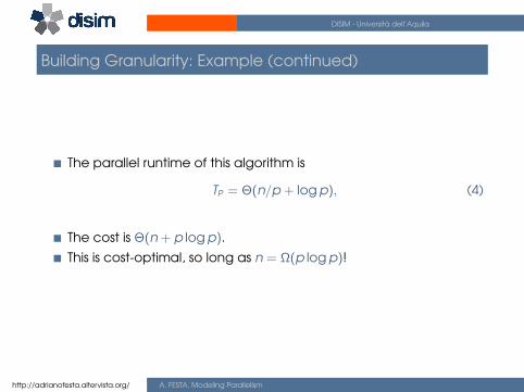
Building Granularity: Example (continued)
The parallel runtime of this algorithm is
TP = Θ(n/p + log p), (4)
The cost is Θ(n + p log p).
This is cost-optimal, so long as n = Ω(p log p)!
http://adrianofesta.altervista.org/ A. FESTA, Modeling Parallelism
DISIM - Universita dell’Aquila
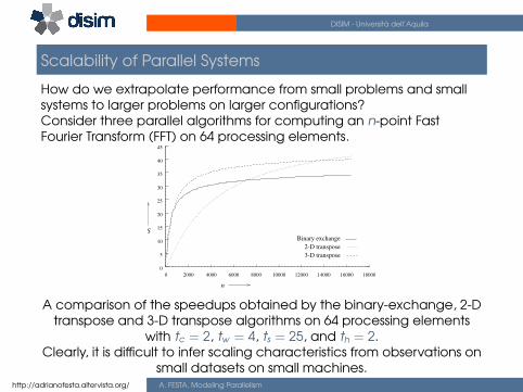
Scalability of Parallel Systems
How do we extrapolate performance from small problems and smallsystems to larger problems on larger configurations?Consider three parallel algorithms for computing an n-point FastFourier Transform (FFT) on 64 processing elements.
180001600014000120001000080006000400020000
0
5
10
15
20
25
30
35
40
45
Binary exchange
2-D transpose
3-D transpose
n
S
A comparison of the speedups obtained by the binary-exchange, 2-Dtranspose and 3-D transpose algorithms on 64 processing elements
with tc = 2, tw = 4, ts = 25, and th = 2.Clearly, it is difficult to infer scaling characteristics from observations on
small datasets on small machines.http://adrianofesta.altervista.org/ A. FESTA, Modeling Parallelism

DISIM - Universita dell’Aquila
Scaling Characteristics of Parallel Programs
The efficiency of a parallel program can be written as:
E =Sp
=TS
pTP
orE =
11 + To
TS
. (5)
The total overhead function To is an increasing function of p.
http://adrianofesta.altervista.org/ A. FESTA, Modeling Parallelism
DISIM - Universita dell’Aquila
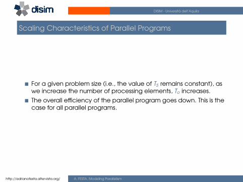
Scaling Characteristics of Parallel Programs
For a given problem size (i.e., the value of TS remains constant), aswe increase the number of processing elements, To increases.
The overall efficiency of the parallel program goes down. This is thecase for all parallel programs.
http://adrianofesta.altervista.org/ A. FESTA, Modeling Parallelism
DISIM - Universita dell’Aquila
Scaling Characteristics of Parallel Programs: Example
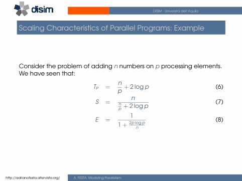
Consider the problem of adding n numbers on p processing elements.We have seen that:
TP =np
+ 2 log p (6)
S =n
np + 2 log p
(7)
E =1
1 + 2p log pn
(8)
http://adrianofesta.altervista.org/ A. FESTA, Modeling Parallelism

DISIM - Universita dell’Aquila
Scaling Characteristics of Parallel Programs: Example
Plotting the speedup for various input sizes gives us:
= 64
= 192
= 320
= 512
0
5
10
15
20
25
30
35
0 5 10 15 20 25 30 35 40
Linear
p
S
n
n
n
n
Speedup versus the number of processing elements for adding a list ofn umbers.
Speedup tends to saturate and efficiency drops as a consequence ofAmdahl’s law.
http://adrianofesta.altervista.org/ A. FESTA, Modeling Parallelism

DISIM - Universita dell’Aquila
Scaling Characteristics of Parallel Programs
Total overhead function To is a function of both problem size TS
and the number of processing elements p.
In many cases, To grows sublinearly with respect to TS .
In such cases, the efficiency increases if the problem size isincreased keeping the number of processing elements constant.
For such systems, we can simultaneously increase the problem sizeand number of processors to keep efficiency constant.
We call such systems scalable parallel systems.
http://adrianofesta.altervista.org/ A. FESTA, Modeling Parallelism

DISIM - Universita dell’Aquila
Scaling Characteristics of Parallel Programs
Recall that cost-optimal parallel systems have an efficiency ofΘ(1).
Scalability and cost-optimality are therefore related.
A scalable parallel system can always be made cost-optimal if thenumber of processing elements and the size of the computationare chosen appropriately.
http://adrianofesta.altervista.org/ A. FESTA, Modeling Parallelism

DISIM - Universita dell’Aquila
Isoefficiency Metric of Scalability
For a given problem size, as we increase the number of processingelements, the overall efficiency of the parallel system goes downfor all systems.
For some systems, the efficiency of a parallel system increases ifthe problem size is increased while keeping the number ofprocessing elements constant.
http://adrianofesta.altervista.org/ A. FESTA, Modeling Parallelism

DISIM - Universita dell’Aquila
Isoefficiency Metric of Scalability
(a) (b)
E
W
Fixed number of processors (p)Fixed problem size (W)
p
E
Variation of efficiency: (a) as the number of processing elements is increased for a given problem size; and (b) as the problem size is
increased for a given number of processing elements. Thephenomenon illustrated in graph (b) is not common to all parallel
systems.
http://adrianofesta.altervista.org/ A. FESTA, Modeling Parallelism

DISIM - Universita dell’Aquila
Isoefficiency Metric of Scalability
What is the rate at which the problem size must increase withrespect to the number of processing elements to keep theefficiency fixed?
This rate determines the scalability of the system. The slower thisrate, the better.
Before we formalize this rate, we define the problem size W as theasymptotic number of operations associated with the best serialalgorithm to solve the problem.
http://adrianofesta.altervista.org/ A. FESTA, Modeling Parallelism
DISIM - Universita dell’Aquila
Isoefficiency Metric of Scalability
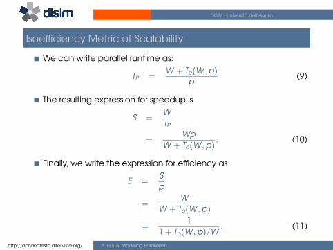
We can write parallel runtime as:
TP =W + To(W ,p)
p(9)
The resulting expression for speedup is
S =WTP
=Wp
W + To(W ,p). (10)
Finally, we write the expression for efficiency as
E =Sp
=W
W + To(W ,p)
=1
1 + To(W ,p)/W. (11)
http://adrianofesta.altervista.org/ A. FESTA, Modeling Parallelism

DISIM - Universita dell’Aquila
Isoefficiency Metric of Scalability
For scalable parallel systems, efficiency can be maintained at afixed value (between 0 and 1) if the ratio To/W is maintained at aconstant value.For a desired value E of efficiency,
E =1
1 + To(W ,p)/W,
To(W ,p)
W=
1− EE
,
W =E
1− ETo(W ,p). (12)
If K = E/(1− E) is a constant depending on the efficiency to bemaintained, since To is a function of W and p, we have
W = KTo(W ,p). (13)
http://adrianofesta.altervista.org/ A. FESTA, Modeling Parallelism
DISIM - Universita dell’Aquila
Isoefficiency Metric of Scalability
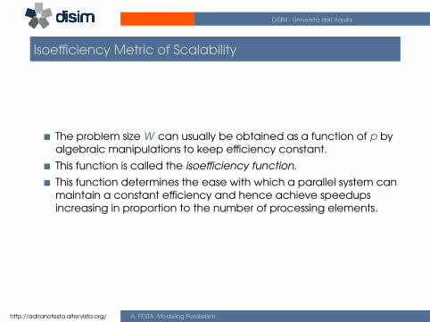
The problem size W can usually be obtained as a function of p byalgebraic manipulations to keep efficiency constant.
This function is called the isoefficiency function.
This function determines the ease with which a parallel system canmaintain a constant efficiency and hence achieve speedupsincreasing in proportion to the number of processing elements.
http://adrianofesta.altervista.org/ A. FESTA, Modeling Parallelism

DISIM - Universita dell’Aquila
Isoefficiency Metric: Example
The overhead function for the problem of adding n numbers on pprocessing elements is approximately 2p log p.
Substituting To by 2p log p, we get
W = K2p log p. (14)
Thus, the asymptotic isoefficiency function for this parallel system isΘ(p log p).
If the number of processing elements is increased from p to p′, theproblem size (in this case, n) must be increased by a factor of(p′ log p′)/(p log p) to get the same efficiency as on p processingelements.
http://adrianofesta.altervista.org/ A. FESTA, Modeling Parallelism

DISIM - Universita dell’Aquila
Isoefficiency Metric: Example
Consider a more complex example where To = p3/2 + p3/4W 3/4.
Using only the first term of To in Equation 13, we get
W = Kp3/2. (15)
Using only the second term, Equation 13 yields the followingrelation between W and p:
W = Kp3/4W 3/4
W 1/4 = Kp3/4
W = K 4p3 (16)
The larger of these two asymptotic rates determines theisoefficiency. This is given by Θ(p3).
http://adrianofesta.altervista.org/ A. FESTA, Modeling Parallelism

DISIM - Universita dell’Aquila
Cost-Optimality and the Isoefficiency Function
A parallel system is cost-optimal if and only if
pTP = Θ(W ). (17)
From this, we have:
W + To(W ,p) = Θ(W )
To(W ,p) = O(W ) (18)
W = Ω(To(W ,p)) (19)
If we have an isoefficiency function f (p), then it follows that therelation W = Ω(f (p)) must be satisfied to ensure the cost-optimalityof a parallel system as it is scaled up.
http://adrianofesta.altervista.org/ A. FESTA, Modeling Parallelism
DISIM - Universita dell’Aquila
Lower Bound on the Isoefficiency Function
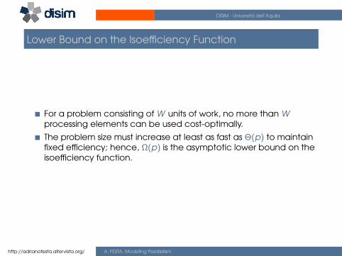
For a problem consisting of W units of work, no more than Wprocessing elements can be used cost-optimally.
The problem size must increase at least as fast as Θ(p) to maintainfixed efficiency; hence, Ω(p) is the asymptotic lower bound on theisoefficiency function.
http://adrianofesta.altervista.org/ A. FESTA, Modeling Parallelism

DISIM - Universita dell’Aquila
Degree of Concurrency and the Isoefficiency Function
The maximum number of tasks that can be executedsimultaneously at any time in a parallel algorithm is called itsdegree of concurrency.
If C(W ) is the degree of concurrency of a parallel algorithm, thenfor a problem of size W , no more than C(W ) processing elementscan be employed effectively.
http://adrianofesta.altervista.org/ A. FESTA, Modeling Parallelism
DISIM - Universita dell’Aquila
Degree of Concurrency and the Isoefficiency Function
Consider solving a system of n equations in n variables by usingGaussian elimination (W = Θ(n3))
The n variables must be eliminated one after the other, andeliminating each variable requires Θ(n2) computations.
At most Θ(n2) processing elements can be kept busy at any time.
Since W = Θ(n3) for this problem, the degree of concurrencyC(W ) is Θ(W 2/3).
Given p processing elements, the problem size should be at leastΩ(p3/2) to use them all.
http://adrianofesta.altervista.org/ A. FESTA, Modeling Parallelism

DISIM - Universita dell’Aquila
Min Execution Time and Min Cost-Optimal Execution Time
Often, we are interested in the minimum time to solution.
We can determine the minimum parallel runtime T minP for a given
W by differentiating the expression for TP w.r.t. p and equating it tozero.
ddp
TP = 0 (20)
If p0 is the value of p as determined by this equation, TP(p0) is theminimum parallel time.
http://adrianofesta.altervista.org/ A. FESTA, Modeling Parallelism

DISIM - Universita dell’Aquila
Minimum Execution Time: Example
Consider the minimum execution time for adding n numbers.
TP =np
+ 2 log p. (21)
Setting the derivative w.r.t. p to zero, we have p = n/2. Thecorresponding runtime is
T minP = 2 log n. (22)
(One may verify that this is indeed a min by verifying that the secondderivative is positive).Note that at this point, the formulation is not cost-optimal.
http://adrianofesta.altervista.org/ A. FESTA, Modeling Parallelism

DISIM - Universita dell’Aquila
Minimum Cost-Optimal Parallel Time
Let T cost optP be the minimum cost-optimal parallel time.
If the isoefficiency function of a parallel system is Θ(f (p)), then aproblem of size W can be solved cost-optimally if and only ifW = Ω(f (p)).
In other words, for cost optimality, p = O(f−1(W )).
For cost-optimal systems, TP = Θ(W/p), therefore,
T cost optP = Ω
(W
f−1(W )
). (23)
http://adrianofesta.altervista.org/ A. FESTA, Modeling Parallelism

DISIM - Universita dell’Aquila
Minimum Cost-Optimal Parallel Time: Example
Consider the problem of adding n numbers.
The isoefficiency function f (p) of this parallel system is Θ(p log p).
From this, we have p ≈ n/log n.
At this processor count, the parallel runtime is:
T cost optP = log n + log
(n
log n
)= 2 log n− log log n. (24)
Note that both T minP and T cost opt
P for adding n numbers areΘ(log n). This may not always be the case.
http://adrianofesta.altervista.org/ A. FESTA, Modeling Parallelism

DISIM - Universita dell’Aquila
Asymptotic Analysis of Parallel Programs
Consider the problem of sorting a list of n numbers. The fastest serialprograms for this problem run in time O(n log n). Consider four parallelalgorithms, A1, A2, A3, and A4 as follows:
Comparison of four different algorithms for sorting a given list ofnumbers. The table shows number of processing elements, parallel
runtime, speedup, efficiency and the pTP product.
Algorithm A1 A2 A3 A4
p n2 log n n√
n
TP 1 n√
n√
n log n
S n log n log n√
n log n√
n
E log nn 1 log n√
n1
pTP n2 n log n n1.5 n log n
http://adrianofesta.altervista.org/ A. FESTA, Modeling Parallelism

DISIM - Universita dell’Aquila
Asymptotic Analysis of Parallel Programs
If the metric is speed, algorithm A1 is the best, followed by A3, A4,and A2 (in order of increasing TP .
In terms of efficiency, A2 and A4 are the best, followed by A3 andA1.
In terms of cost, algorithms A2 and A4 are cost optimal, A1 and A3are not.
It is important to identify the objectives of analysis and to useappropriate metrics!
http://adrianofesta.altervista.org/ A. FESTA, Modeling Parallelism

DISIM - Universita dell’Aquila
Other Scalability Metrics
A number of other metrics have been proposed, dictated byspecific needs of applications.
For real-time applications, the objective is to scale up a system toaccomplish a task in a specified time bound.
In memory constrained environments, metrics operate at the limitof memory and estimate performance under this problem growthrate.
http://adrianofesta.altervista.org/ A. FESTA, Modeling Parallelism