ANALYTICAL TRILINEAR PRESSURE TRANSIENT MODEL FOR

MULTIPLY FRACTURED HORIZONTAL WELLS IN TIGHT SHALE

RESERVOIRS

by

Margaret L. Brown

ii

A thesis submitted to the Faculty and the Board of Trustees of the Colorado School of

Mines in partial fulfillment of the requirements for the degree of Master of Science

(Petroleum Engineering).

Golden, Colorado

Date: ____________________

Signed:____________________________

Margaret L. Brown

Signed:____________________________

Dr. Erdal Ozkan Thesis Advisor

Golden, Colorado

Date: ____________________

Signed:____________________________

Dr. Ramona Graves Professor and Head

Department of Petroleum Engineering

iii

ABSTRACT

This research presents an analytical model to obtain the pressure transient

response of multiply fractured horizontal wells in tight shale formations – the trilinear

model. The solution procedure is based on prior analytic models developed for fractured

vertical wells in layered reservoirs and fractured horizontal wells in conventional

formations. The model derivation is presented in its most general form and modifications

to account for naturally fractured media, as well as gas flow, flow choking at the

wellbore, and wellbore storage are all presented.

The new trilinear model is verified against an existing semianalytical solution.

The verification procedure highlighted the impact of different dual porosity models in

obtaining a good match on field data. Asymptotic approximations are presented including

a discussion on their usefulness in straight-line analysis. A field example demonstrates

the usefulness of the new model. Parameters relating to the productivity of a multiply

fractured horizontal well in a tight shale formation are then explored using the trilinear

model. It is determined that relatively high matrix permeability and high hydraulic

fracture conductivity are not sufficient to accomplish favorable productivities in shale

reservoirs, unlike in conventional reservoirs. It is also determined that the most efficient

mechanism to improve the productivity of tight, shale formations is to increase the

density of the natural fractures. Increasing the permeability of the natural fractures has an

insignificant effect. Similarly, decreasing hydraulic fracture spacing increases the

productivity of the well, but the incremental gain for each additional fracture decreases.

iv

It is demonstrated that the key characteristics of flow convergence toward a

multiply fractured horizontal well in a shale reservoir may be preserved in the relatively

simple analytical trilinear model. Moreover, with minimal computational time, the

trilinear model describes parameters contributing to the productivity of fractured

horizontal wells and allows for performance characteristics of multiply fractured

horizontal wells to be delineated.

v

TABLE OF CONTENTS

ABSTRACT ............................................................................................................... iii

LIST OF FIGURES .................................................................................................... vii

LIST OF TABLES ...................................................................................................... ix

ACKNOWLEDGEMENT ............................................................................................ x

CHAPTER 1 INTRODUCTION ................................................................................... 1

1.1 Motivation .......................................................................................................... 1

1.2 Background ........................................................................................................ 3

1.3 Problem Statement .............................................................................................. 6

1.4 Objectives .......................................................................................................... 8

1.5 Method of Study ................................................................................................. 9

1.6 Contributions of the Study ................................................................................. 10

1.7 Organization of the Thesis ................................................................................. 11

CHAPTER 2 LITERATURE REVIEW ...................................................................... 13

CHAPTER 3 MATHEMATICAL MODEL ................................................................ 22

3.1 Trilinear Flow Model Assumptions ................................................................... 23

3.2 Definitions ........................................................................................................ 27

3.3 Derivation of the Analytic Solution ................................................................... 29

3.3.1 The Outer Reservoir Solution ..................................................................... 29

3.3.2 The Inner Reservoir Solution ...................................................................... 32

3.3.3 The Hydraulic Fracture Solution ................................................................. 38

3.4 Dual Porosity Parameters .................................................................................. 44

3.5 Gas ................................................................................................................... 48

3.6 Choking ............................................................................................................ 49

3.7 Wellbore Storage .............................................................................................. 50

CHAPTER 4 MODEL VERIFICATION ..................................................................... 52

4.1 Model Verification ............................................................................................ 53

4.2 Impact of Choice in Dual Porosity Models ......................................................... 58

vi

4.3 Asymptotic Approximations and Flow Regimes ................................................. 61

4.3.1 Early-Time Asymptotic Solution ................................................................. 62

4.3.2 Intermediate-Time Asymptotic Solutions .................................................... 62

4.3.3 Late-Time Asymptotic Solutions ................................................................. 65

4.4 Field Example ................................................................................................... 67

CHAPTER 5 ANALYSIS OF RESULTS .................................................................... 74

5.1 Effect of the Outer Reservoir ............................................................................. 75

5.2 Effect of Matrix Permeability ............................................................................ 79

5.3 Effect of Natural Fracture Permeability and Density ........................................... 85

5.4 Effect of Hydraulic Fracture Permeability and Spacing ...................................... 88

5.5 Computation of the Productivity Index .............................................................. 93

CHAPTER 6 CONCLUSIONS AND RECOMMENDATIONS ................................... 95

6.1 Conclusions ...................................................................................................... 95

6.2 Recommendations ............................................................................................. 98

NOMENCLATURE ................................................................................................... 99

REFERENCES CITED ............................................................................................ 103

vii

LIST OF FIGURES

Figure 1.1 – Single hydraulic fracture and the definition of conductivity. ....................... 3 Figure 1.2 – Multiply fractured horizontal-well in a conventional tight formation and the

effective, or total, fracture concept. ........................................................................ 4 Figure 1.3 – Effective wellbore radius versus effective system conductivity for a multiply

fractured horizontal well in a conventional tight reservoir (after Raghavan et al., 1997). ................................................................................................................... 5

Figure 1.4 – Effective fracture concept for a multiply fractured horizontal well in an

unconventional tight shale reservoir. ...................................................................... 8 Figure 3.1 – Schematic of the trilinear flow model representing three contiguous flow

regions for a multiply fractured horizontal well. ................................................... 24 Figure 3.2 – Multiply fractured horizontal well and the symmetry element used in

deriving the trilinear flow model. ........................................................................ 26 Figure 4.1 – Comparison of the trilinear and semianalytical model (Medeiros et al. , 2008)

results without wellbore storage. ......................................................................... 56 Figure 4.2 – Comparison of the trilinear and semianalytical model (Medeiros et al. , 2008)

results with wellbore storage. .............................................................................. 58 Figure 4.3 – Comparison, using the trilinear model, of the pseudosteady and transient

dual porosity models for a naturally fractured inner reservoir. .............................. 59 Figure 4.4 – Using the trilinear model to analyze the effect of wellbore storage on

pseudosteady and transient dual porosity models for a naturally fractured inner reservoir. ............................................................................................................ 60

Figure 4.5 – Trilinear model match of the field data. .................................................... 68 Figure 4.6 – Flow rate history before shut-in for the field example. .............................. 71 Figure 4.7 – Comparison of drawdown and buildup results for the analysis of field data.

.......................................................................................................................... 72

viii

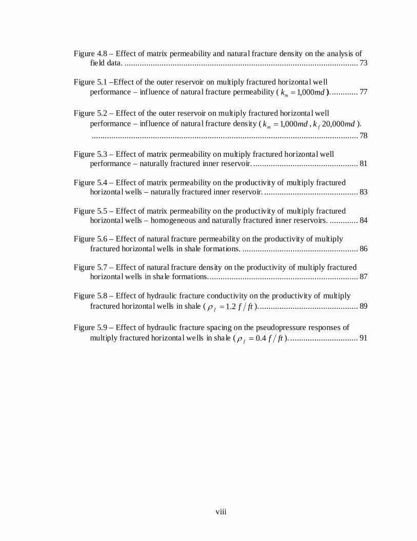
Figure 4.8 – Effect of matrix permeability and natural fracture density on the analysis of field data. ........................................................................................................... 73

Figure 5.1 –Effect of the outer reservoir on multiply fractured horizontal well

performance – influence of natural fracture permeability ( mdkm 000,1= ). ............ 77 Figure 5.2 – Effect of the outer reservoir on multiply fractured horizontal well

performance – influence of natural fracture density ( mdkm 000,1= , mdk f 000,20 ). .......................................................................................................................... 78

Figure 5.3 – Effect of matrix permeability on multiply fractured horizontal well

performance – naturally fractured inner reservoir. ................................................ 81 Figure 5.4 – Effect of matrix permeability on the productivity of multiply fractured

horizontal wells – naturally fractured inner reservoir. ........................................... 83 Figure 5.5 – Effect of matrix permeability on the productivity of multiply fractured

horizontal wells – homogeneous and naturally fractured inner reservoirs. ............. 84 Figure 5.6 – Effect of natural fracture permeability on the productivity of multiply

fractured horizontal wells in shale formations. ..................................................... 86 Figure 5.7 – Effect of natural fracture density on the productivity of multiply fractured

horizontal wells in shale formations. .................................................................... 87 Figure 5.8 – Effect of hydraulic fracture conductivity on the productivity of multiply

fractured horizontal wells in shale ( ftff 2.1=ρ ). ............................................. 89 Figure 5.9 – Effect of hydraulic fracture spacing on the pseudopressure responses of

multiply fractured horizontal wells in shale ( ftff 4.0=ρ ). ............................... 91

ix

LIST OF TABLES

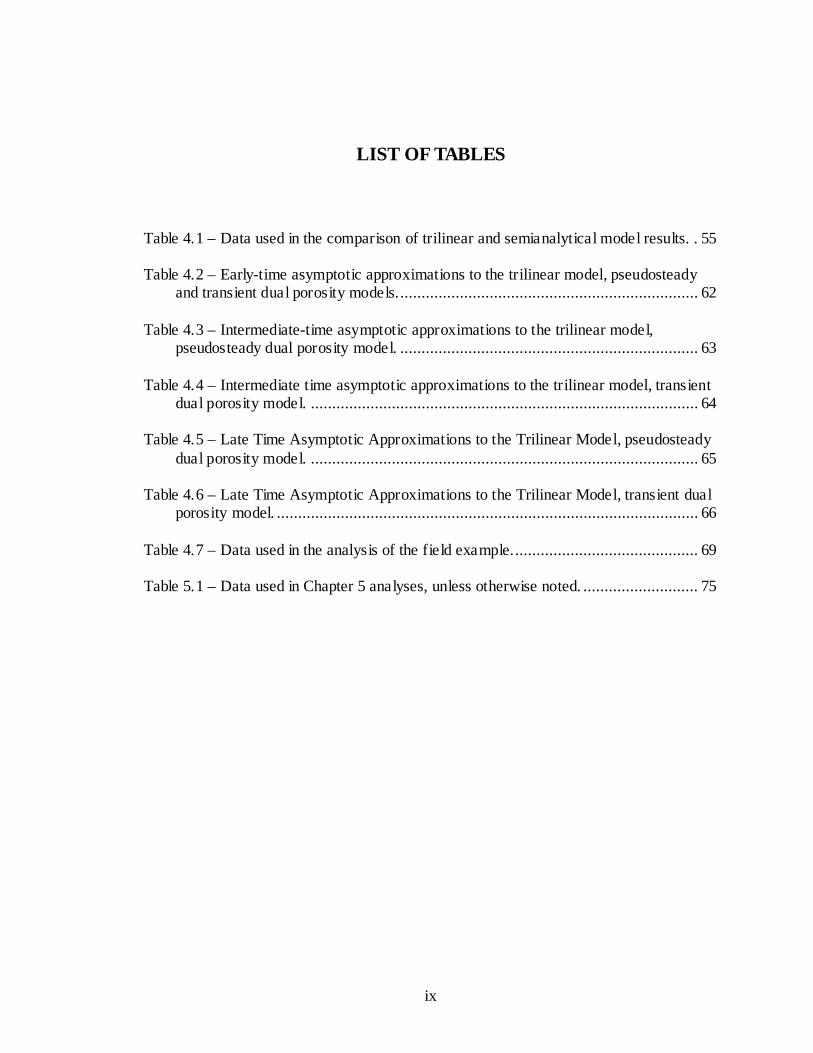
Table 4.1 – Data used in the comparison of trilinear and semianalytical model results. . 55 Table 4.2 – Early-time asymptotic approximations to the trilinear model, pseudosteady

and transient dual porosity models. ...................................................................... 62 Table 4.3 – Intermediate-time asymptotic approximations to the trilinear model,

pseudosteady dual porosity model. ...................................................................... 63 Table 4.4 – Intermediate time asymptotic approximations to the trilinear model, transient

dual porosity model. ........................................................................................... 64 Table 4.5 – Late Time Asymptotic Approximations to the Trilinear Model, pseudosteady

dual porosity model. ........................................................................................... 65 Table 4.6 – Late Time Asymptotic Approximations to the Trilinear Model, transient dual

porosity model. ................................................................................................... 66 Table 4.7 – Data used in the analysis of the field example. ........................................... 69 Table 5.1 – Data used in Chapter 5 analyses, unless otherwise noted. ........................... 75

x

ACKNOWLEDGEMENT

I would like to acknowledge my advisor, Dr. Erdal Ozkan – without his guidance

and assistance, the process of conducting this research study, and indeed navigating my

entire degree program, would have been exponentially more difficult. Ever-gracious, Dr.

Hossein Kazemi has provided me with endless, and sometimes unwarranted, praise and

encouragement throughout this entire study! Both gentlemen have afforded me many

opportunities that would not have otherwise been available to me for which I would like

to express my utmost gratitude. I would like to thank Dr. Jennifer Miskimins for her time

and also for the more practical focus I have developed on this research as a result of

discussions I have had with her students.

Denise Winn-Bower deserves a special thank you for all of her work on behalf of

the Marathon Center of Excellence for Reservoir Studies including, but certainly not

limited to, trying to keep me organized. I would like to say thanks to: Najeeb Alharthy,

Mohammed Al-Kobaisi, Juan Carlos Carratu Ramos, Basak Kurtoglu, and Dr. Flavio

Medeiros, my fellow graduate students at MCERS, all of whom have helped me greatly.

Furthermore, I acknowledge the financial support I received from MCERS in pursuit of

my Masters thesis.

Finally, I would like to thank my parents, Tom and Sally Brown. Throughout this

entire process they have helped me keep my head screwed on straight – no small task.

Their unfailing support and occasional criticism was exactly what I needed in order to

accomplish my Master of Science degree at Colorado School of Mines. I love you both!

1

CHAPTER 1

INTRODUCTION

This thesis presents work performed for a Master of Science degree that was

conducted at the Marathon Center of Excellence for Reservoir Studies in the Petroleum

Engineering Department of the Colorado School of Mines. The MSc research presented

herein develops an analytic model, the trilinear model, describing a system composed of

a multiply fractured horizontal well in a tight shale reservoir which may or may not be

naturally fractured. The trilinear model is new and constitutes the significant contribution

of this research. The following sections present the motivation behind the study as well as

the objectives, background, approach, and organization of the remainder of the thesis.

1.1 Motivation

With maturity, the oil and gas industry has moved into developing resources of

greater and greater complexity. Shale reservoirs of very low permeability are one such

resource. Once looked upon as any rock that was not reservoir quality, shales have now

become viable reservoirs in their own right. A classic definition of shale is a class of fine-

grained clastic sedimentary rocks with a mean grain size of less than 0.0625 mm ,

including siltstone, mudstone, and claystone (EIA 2006). Recent literature (Kundert and

Mullen, 2009) has noted that, with the industry’s expanding exploration in shale plays,

2

the boundaries of what constitutes shale have also been expanded and now include

reservoir rock within a wide range of total organic content (TOC) and maturity.

Regardless, the goal behind developing a shale formation is to maximize the

surface area available to flow. To this end, horizontal wells are frequently drilled through

the reservoir and completed with some number of hydraulic fractures, creating a multiply

fractured horizontal well. The horizontal well may run for hundreds or thousands of feet

through the formation and the hydraulic fractures open transverse, longitudinal, or

complex planes out into the formation. Frequently during the hydraulic fracturing

process, a system of smaller fractures is either created or reactivated, dependant upon a

preexisting natural fracture network. These smaller fractures that propagate through the

tight matrix between the hydraulic fractures add significantly to the system’s ability to

flow – they add to the effective permeability of the matrix.

This is a complex system. How then can it be modeled? Certainly it is possible to

develop detailed numerical models, as presented by Medeiros et al. (2008) for example,

to model transient fluid flow toward a multiply fractured horizontal well in an

unconventional reservoir. There are downsides to these models, however: the increased

computational requirements, the implicit functional relationships of key parameters, and

the inconvenience in their use in iterative applications.

This work proposes to develop a simple analytical model that accurately

represents the system described above while enabling iterative applications for design

purposes with minimal computational time. Despite the complex interplay of flow among

matrix, natural fractures, and hydraulic fractures, the key characteristics of flow

convergence toward a horizontal well stimulated by multiple transverse fractures may be

3

preserved in a relatively simple, trilinear flow model. The basis of the trilinear flow

model is the premise that the productive lives of fractured horizontal wells in shale

formations are dominated by linear flow regimes (Medeiros et al., 2008).

1.2 Background

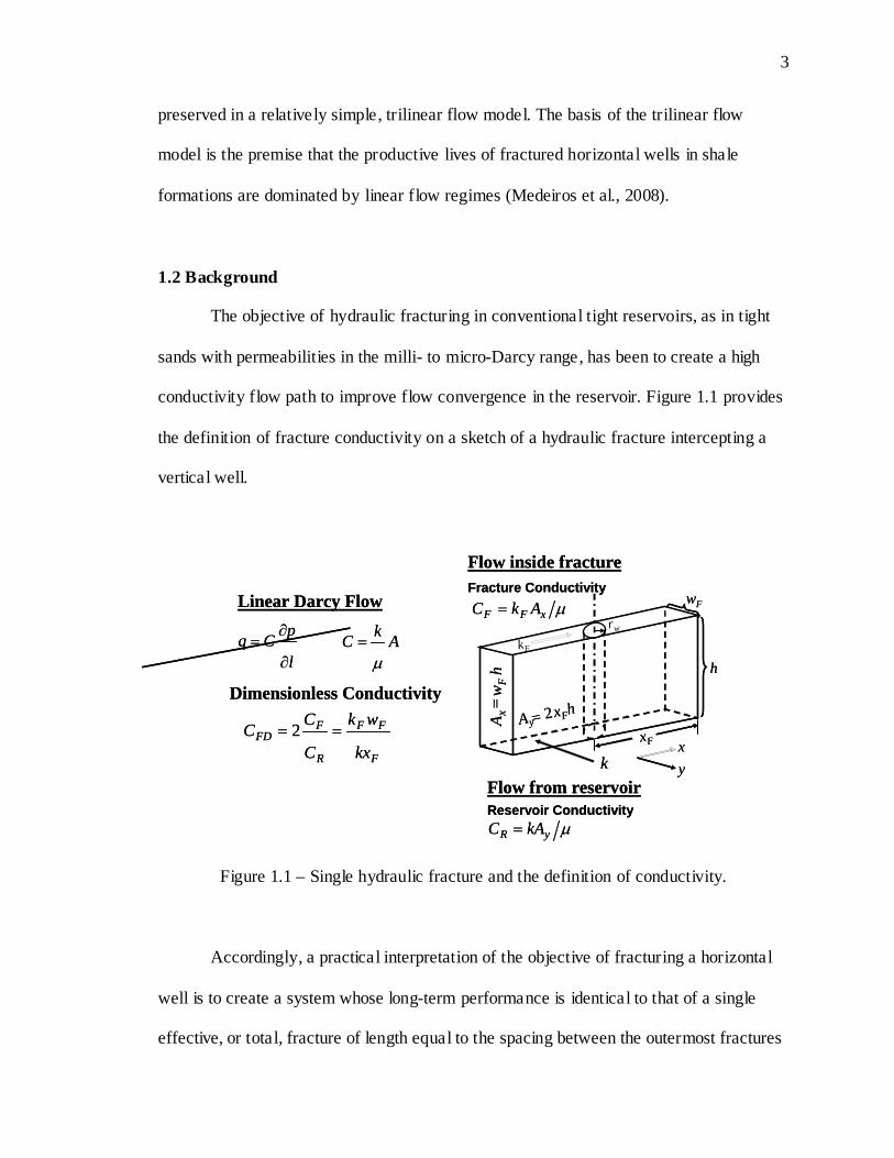
The objective of hydraulic fracturing in conventional tight reservoirs, as in tight

sands with permeabilities in the milli- to micro-Darcy range, has been to create a high

conductivity flow path to improve flow convergence in the reservoir. Figure 1.1 provides

the definition of fracture conductivity on a sketch of a hydraulic fracture intercepting a

vertical well.

rw

xF

wF

h

xy

Flow inside fractureFracture Conductivity

Flow from reservoirReservoir Conductivity

µxFF AkC =

µyR kAC =

hxFAy2=

hw

FA x

=

k

kF

Dimensionless Conductivity

l

pCq∂

∂=

F

FF

R

FFD

kx

wk

C

CC == 2

Linear Darcy Flow

AkCµ

=rw

xF

wF

h

xy

Flow inside fractureFracture Conductivity

Flow from reservoirReservoir Conductivity

µxFF AkC =

µyR kAC =

hxFAy2=

hw

FA x

=

k

kF

Dimensionless Conductivity

l

pCq∂

∂=

F

FF

R

FFD

kx

wk

C

CC == 2

Linear Darcy Flow

AkCµ

=

Figure 1.1 – Single hydraulic fracture and the definition of conductivity.

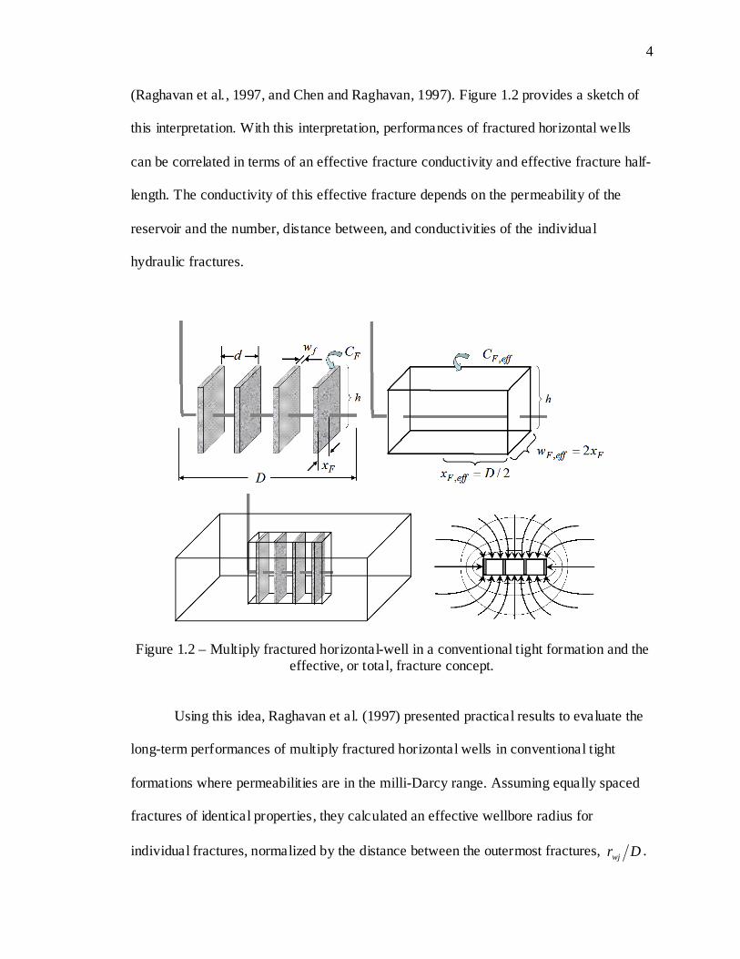
Accordingly, a practical interpretation of the objective of fracturing a horizontal

well is to create a system whose long-term performance is identical to that of a single

effective, or total, fracture of length equal to the spacing between the outermost fractures

4

(Raghavan et al. , 1997, and Chen and Raghavan, 1997). Figure 1.2 provides a sketch of

this interpretation. With this interpretation, performances of fractured horizontal wells

can be correlated in terms of an effective fracture conductivity and effective fracture half-

length. The conductivity of this effective fracture depends on the permeability of the

reservoir and the number, distance between, and conductivities of the individual

hydraulic fractures.

Figure 1.2 – Multiply fractured horizontal-well in a conventional tight formation and the effective, or total, fracture concept.

Using this idea, Raghavan et al. (1997) presented practical results to evaluate the

long-term performances of multiply fractured horizontal wells in conventional tight

formations where permeabilities are in the milli-Darcy range. Assuming equally spaced

fractures of identical properties, they calculated an effective wellbore radius for

individual fractures, normalized by the distance between the outermost fractures, Drwj .

5

Using this effective wellbore radius concept, Raghavan et al. (1997) correlated the long-

term performances of multiply fractured horizontal wells, after the onset of pseudoradial

flow, with the effective, or total, system conductivity ( fDteffectveFD CC =, ). The Raghavan et

al. (1997) correlation, shown in Fig. 1.3, is similar to the correlation presented by Cinco

et al. (1978) to obtain the effective wellbore radius of a single fracture as a function of

fracture conductivity and half-length.

Figure 1.3 – Effective wellbore radius versus effective system conductivity for a multiply fractured horizontal well in a conventional tight reservoir (after Raghavan et al., 1997).

As shown in Fig. 1.3, the Raghavan et al. (1997) correlation includes multiple

curves for different numbers of fractures along the well. The top curve in Fig. 1.3

represents the Cinco et al. (1978) correlation for a single fracture. Figure 1.3 can be used

to determine the effective, or total, system conductivity, fDteffectveFD CC =, , for given

individual fracture properties such as conductivity, FDC , half-length, Fx , distance

6

between the outermost fractures, D , and the number of fractures along the well, Fn .

Then, using the effective system conductivity, effectiveFDC , , and half-length,

2, Dx effectiveF = , effective wellbore radius, wteffectivew rr =, , of the total system is obtained

from the Cinco et al. correlation.

As noted by Chen and Raghavan (1997), the total effective wellbore radius can be

used in the following well-known deliverability equation:

( )

−×=

−

2,

3

4ln21

~1008.7

effectivewA

wf

rCeA

ppB

khq

γ

µ. (1.1)

Then, using Fig. 1.3 and Eq. 1.1, it is possible to design a multiply fractured

horizontal well to accomplish the desired productivity. Given a set of hydraulic fracture

properties, for example, it is possible to optimize the number of fractures along the length

of a horizontal well. Similarly, the optimum number of fractures, the length of the

horizontal well, and the properties of the hydraulic fractures required to drain a given

reservoir of area A , and shape as determined by the shape factor AC , can be found from

Fig. 1.3 and Eq. 1.1.

1.3 Problem Statement

It must be emphasized, however, that the approach detailed above may only be

used if the performance of the multiply fractured horizontal well is dominated by the

long-term productivity of the reservoir beyond the tips of the fractures and the horizontal

well. In other words, pseudoradial flow convergence must develop around the multiply

fractured horizontal well for the effective wellbore radius concept to be used.

7

Pseudoradial flow develops around a single infinite conductivity vertical fracture for

times (Gringarten et al. , 1974)

k

xct Ft

241014.1 µφ×≥ . (1.2)

For long fractures, with large values of Fx , and tight formations, with small

values of k , the time until the start of pseudoradial flow may be very long. In multiply

fractured horizontal wells, Fx in Eq. 1.2 corresponds to 2, Dx effectiveF = – frequently a

very large number. Therefore, the start of pseudoradial flow in multiply fractured

horizontal wells may be delayed for even moderate permeabilities. As such, most of the

productive life of a fractured horizontal well in a shale formation is dominated by

transient production from the stimulated volume between the hydraulic fractures

(Raghavan et al. , 1997). In fact, for reservoir properties typically encountered in practical

multiply fractured horizontal well applications in shale, flow convergence hardly occurs

beyond the tips of the fractures. Therefore, the productivity of multiply fractured

horizontal wells is dominated by linear flow perpendicular to the fracture surfaces

confined to the stimulated volume between the fractures.

Developing a model to describe this linear flow convergence in a multiply

fractured horizontal well in a shale formation is the main problem addressed by this

thesis. Under these conditions, the long-term performance of a fractured horizontal well

and reservoir system may again be represented by that of a single hydraulic fracture. The

length of the equivalent hydraulic fracture is equal to the aggregate length of the

hydraulic fractures and the conductivity of the equivalent fracture is equal to the average

of the conductivities of the individual fractures, as shown in Fig. 1.4. The drainage

8

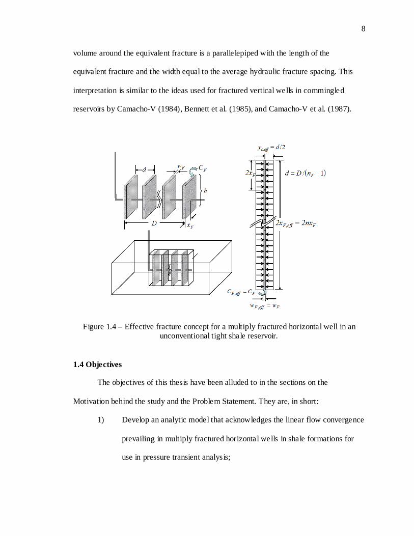
volume around the equivalent fracture is a parallelepiped with the length of the

equivalent fracture and the width equal to the average hydraulic fracture spacing. This

interpretation is similar to the ideas used for fractured vertical wells in commingled

reservoirs by Camacho-V (1984), Bennett et al. (1985), and Camacho-V et al. (1987).

Figure 1.4 – Effective fracture concept for a multiply fractured horizontal well in an unconventional tight shale reservoir.

1.4 Objectives

The objectives of this thesis have been alluded to in the sections on the

Motivation behind the study and the Problem Statement. They are, in short:

1) Develop an analytic model that acknowledges the linear flow convergence

prevailing in multiply fractured horizontal wells in shale formations for

use in pressure transient analysis;

9

2) The model should be relatively simple while still capturing the key

characteristics of flow convergence due to the complex nature of flow

between the matrix, natural fractures, and the hydraulic fractures;

3) With minimal computational time, the model should enable iterative

applications for purposes of designing fracture treatments; and

4) The model should describe the parameters contributing to the productivity

of fractured horizontal wells and allow for performance characteristics of

multiply fractured horizontal wells in shale to be delineated.

1.5 Method of Study

The method of this research is analytical. For the general trilinear model,

presented in detail in Chapter 3, solutions to the diffusion equation, a differential

equation, were derived in three separate but linked reservoir sections: the outer reservoir,

the inner reservoir, and the hydraulic fracture. Each reservoir section is distinct from the

others and internally homogeneous. As such, each section is characterized by uniform

average properties specific to the section. The sections were linked together by

recognizing the continuity of pressure at mutual boundaries. Due to the nature of the

system most typically found in practical applications, the inner reservoir is allowed to be

naturally fractured. For the naturally fractured inner zone, a dual porosity idealization

was used to represent flow in the fractures and the matrix. Either the pseudosteady dual

porosity model (Warren and Root, 1963) or the transient dual porosity model (Kazemi,

1969, de Swaan-O, 1976, Serra et al., 1983) may be used. Solutions to the diffusion

equation were derived in the Laplace domain and, because all of the functions in this

10

work are continuous, the Stehfest algorithm (1970) was used to numerically invert the

results back into the time domain.

The computational code was written in FORTRAN 90. Results from the trilinear

model were verified against a semianalytical solution available in the literature (Mederios

2007). Asymptotic approximations were derived for the general solution to determine

limiting forms of the equation. The trilinear model was then used in both theoretical and

practical applications to determine sensitivities as well as elucidating important

considerations when designing a multiply fractured horizontal well system in a shale

formation.

1.6 Contributions of the Study

This thesis presents an analytical trilinear flow solution to simulate the pressure

transient and production behavior of fractured horizontal wells in shale reservoirs. The

trilinear model constitutes the primary new contribution of this thesis.

There are several aspects of the trilinear model worth highlighting. By taking

advantage of the predominately linear flow in systems of this nature, the trilinear model

is much simpler than existing semianalytical and numerical models, but still versatile

enough to incorporate the fundamental petrophysical characteristics of shale reservoirs,

including the intrinsic properties of the matrix and the natural fractures. This practical

solution provides an excellent alternative to rigorous solutions, which are cumbersome to

evaluate. This new, simpler, trilinear model is therefore useful for solving optimization

problems and, by extension, useful for design purposes. It may also be useful for

pressure transient analysis and rate transient analysis software packages.

11

The various analyses made possible by the trilinear model that are included in this

thesis help to ground some field observations in theory as well as highlight possible areas

for improving design processes for fracture treatments of multiply fractured horizontal

wells in shale formations – both are also contributions of the study.

1.7 Organization of the Thesis

This thesis is divided into six chapters. This chapter, Chapter 1, is the introduction

and contains the motivation behind the study as well as the background to the study. It

also contains a discussion on how the study was conducted and the main contributions of

the study.

Chapter 2 presents a review of the literature pertinent to the development of this

thesis.

Chapters 3, 4, and 5 constitute the meat of the thesis. The derivation of the

analytical trilinear model is presented in Chapter 3, followed by sections addressing

modifications necessary to the trilinear model to accommodate for naturally fractured

systems, gas flow, choking, and wellbore storage effects. Chapter 4 presents a

verification of the trilinear model, a discussion on the impact of different dual porosity

models on the analysis, a presentation of asymptotic approximations, including a

discussion as to their usefulness in straight-line analysis, and finally, a field example.

Chapter 5 puts forth results and general observations made possible by the trilinear model

on the nature of productivity and flow in multiply fractured horizontal wells in shale

reservoirs.

12

The final chapter, Chapter 6, makes recommendations for future research to

extend the work started in this thesis and provides the main conclusions resulting from

the work described herein.

13

CHAPTER 2

LITERATURE REVIEW

Developing an analytical model to describe a complex system is beneficial

because of the relative simplicity of these types of models. This simplicity lends itself to

fewer input parameters, therefore easing data collection requirements. For equivalent

systems, results from analytical models may also be obtained much more quickly than

those from numerical models. The complex system addressed in this thesis is a

hydraulically fractured horizontal well with a naturally fractured inner reservoir and a

tight outer reservoir. The solution presented herein is based on prior work in the areas of

fluid flow in porous media, naturally fractured reservoirs, hydraulically fractured wells,

horizontal wells, and tight gas reservoirs.

The seminal work of Carslaw and Jaeger (1959) is recognized for its

documentation of and contribution to the solutions and solution techniques of three-

dimensional heat conduction problems. The foundations and wide variety of applications

for the solution techniques presented by Carslaw and Jaeger are also used to solve

problems relating to fluid flow in porous media: Green’s functions, sources and sinks,

and Laplace transformation are among the most common techniques. For example, as

introduced to the petroleum engineering literature by Van Everdingen and Hurst in 1949,

Laplace transformation is integral to the solution of analytical models based on the

diffusion equation. In the Laplace domain, variable flow rate boundary conditions,

14

constant pressure production, wellbore storage, and some forms of reservoir

heterogeneity, such as natural fractures, may all be dealt with easily. Asymptotic

approximations are also easily derived from solutions presented in the Laplace domain.

Using numerical inversion algorithms, like Stehfest’s algorithm (1970), results computed

in the Laplace domain may also be inverted back into the time domain when an analytical

inversion is not possible or convenient.

In general, analytical solution techniques are applicable to the linearized form of

diffusion equation, which assumes constant properties. The assumption of constant

properties works well for oil and water systems where compressibility and viscosity may

be assumed to be independent of pressure. Clearly, gas properties are not independent of

pressure, and therefore the diffusivity equation for gas is nonlinear. To extend the

analytical solutions derived for oil and water to gas, Al-Hussainy and Ramey (1966) and

Al-Hussainy et al. (1966) introduced the idea of real gas pseudopressure. Real gas

pseudopressure is a process by which the diffusivity equation for gas is linearized using a

variable transformation.

In the Laplace domain, the solution to the diffusion equation for naturally

fractured reservoirs is easily obtained using either of two dual porosity idealizations. The

dual porosity model presented by Warren and Root (1963) considers pseudosteady fluid

transfer from the matrix to the fracture. Usually, this pseudosteady dual porosity model is

introduced in terms of bulk properties, and characteristics of the matrix and fracture

media are incorporated into the model by two ratios: the storativity and the

transmissivity. The storativity ratio is a measure of the quantity of fluid that the natural

fractures can store to that which the combined system, both the matrix and the fractures,

15

can store. On the other hand, the transmissivity ratio is a measure of flow capacity

between the matrix and the factures. A matrix shape factor is also introduced with the

transmissivity ratio that addresses the geometry of the individual matrix blocks. Kazemi

(1976) provided a good first approximation for this matrix shape factor.

Kazemi (1969) analyzed the pseudosteady dual porosity model of Warren and

Root (1963) using transient flow at all times and extended the complexity of the model

into two dimensions. In addition to defining a matrix shape factor, Kazemi (1976) also

added multiphase flow to the bones of the Warren and Root (1963) model, which allowed

for water/oil flow. Similarly, deSwaan-O (1976) developed an alternative dual porosity

model that considered transient fluid transfer from the matrix to the fracture. The model

proposed by deSwaan-O assumed a uniform fracture distribution, specifically, parallel

horizontal fractures that are equally spaced from one another. Unlike the Warren and

Root (1963) model, the transient model may be introduced in terms of either intrinsic or

bulk properties of the fracture and matrix media. Serra, et al. (1983) represented the

naturally fractured reservoir as a stack of alternating matrix and fracture slabs and

presented the transient dual porosity model in terms of intrinsic parameters. As such,

Serra, et al. (1983) redefined the storativity ratio to be a ratio of the quantity of fluid that

the natural fractures can store to that which only the matrix may store.

Moving from naturally fractured reservoirs, Prats (1961) and Prats et al. (1962)

investigated the behavior of hydraulically fractured vertical wells and identified the

fundamental flow behaviors. They showed that dimensionless well responses could be

correlated in terms of dimensionless fracture conductivity. Gringarten et al.(1974)

presented a solution for an infinite-conductivity vertical fracture intercepting a vertical

16

well. The authors also developed an equation to determine the time at which pseudoradial

flow develops around a single infinite conductivity vertical fracture. Using the solution

developed by Gringarten et al. (1974), Gringarten et al. (1975) presented type curves to

analyze transient pressure behavior of infinite conductivity hydraulic fractures. Cinco-

Ley et al. (1978) extended the solution presented by Gringarten et al. (1974) to

investigate hydraulically fractured vertical wells with a finite conductivity vertical

fracture. Similar to Prats (1961) and Prats et al. (1962), they correlated dimensionless

wellbore pressure in terms of dimensionless fracture conductivity. Dimensionless fracture

conductivity is comprised of the effects of width, permeability, and half-length of the

vertical fracture along with the matrix permeability. Plotting the log of dimensionless

wellbore pressure against the log of dimensionless time yielded a family of characteristic

curves that enabled the determination of formation and fracture characteristics. These

curves demonstrated that for dimensionless conductivity values over 300, the finite

conductivity vertical fracture solution behaved similarly to the infinite conductivity

vertical fracture solution of Gringarten et al. (1974). Cinco-Ley and Sameniego (1981)

used the hydraulically fractured well solution of Cinco-Ley et al. (1978) and documented

the characteristics of flow regimes and pressure transient analysis procedures. They

identified a bilinear flow regime, where linear flows from the matrix to the fracture and

from the fracture to the wellbore occur simultaneously. Bilinear flow is observable on a

log-log plot of dimensionless wellbore pressure against dimensionless time by fitting a

straight line possessing a one-quarter slope to the data. Further, the authors observed that,

during bilinear flow, a plot of dimensionless wellbore pressure and the fourth root of

17

dimensionless time resulted in a straight line that was inversely proportional to fracture

conductivity.

Bennett et al. (1985) put forth a procedure for obtaining analytic pressure

transient solutions for fractured vertical wells in layered reservoirs. In this solution

procedure the idea of dimensionless reservoir conductivity is presented – a parameter that

relates flow from one layer of a reservoir to the average reservoir properties. Camacho-C

et al. (1987) used similar solution procedures to obtain analytic pressure transient

solutions for fractured vertical wells in layered reservoirs where the vertical fractures

were of unequal length. Using the concept of an effective system conductivity, Camacho-

C et al. (1987) demonstrate that multi-layer solutions can be correlated with single layer

solutions if the sum of the product of the dimensionless layer conductivity and fracture

half-length for each layer replace the fracture half-length term in the single layer

solutions.

Cinco and Meng (1988) extended the earlier work on finite conductivity vertical

fractures intercepting a vertical well and naturally fractured reservoirs. They presented an

analytical solution in Laplace domain for a finite conductivity fractured vertical well in a

dual porosity system, using both the pseudosteady and the transient dual porosity

idealizations. Their work demonstrated that the behavior of the total system could be

represented by a combination of the behavior of a finite conductivity fractured vertical

well in a homogeneous reservoir and the behavior of a vertical well in a dual porosity

reservoir. The authors also observed a flow phenomenon that they referred to as trilinear

flow – where matrix linear flow was overlaid with bilinear flow in the hydraulic fracture.

18

The trilinear flow regime was seen on a log-log plot of pressure versus time,

characterized by portion of the data forming a straight line and having a th81 slope.

Soliman et al. (1990) explored the pressure transient behavior of fractured

horizontal wells in tight formations and presented a method by which the optimal number

of fractures for a horizontal well could be determined, concluding that an understanding

of the natural fracture network was crucial to optimizing hydraulic fracture design even

when the conductivity of the hydraulic fractures was assumed to be infinite. The authors

also observed a very early time radial flow convergence from the hydraulic fracture to the

horizontal wellbore that caused an increased pressure drop. To approximate this

additional pressure drop due to radial flow convergence in the fracture, Mukherjee and

Economides (1991) developed a flow choking skin factor. The choking skin factor may

simply be added to the linear flow solution as a good approximation for dimensionless

wellbore pressure after the end of radial flow in the hydraulic fracture. Larsen and Hegre

(1991) developed an analytical pressure transient solution for a finite conductivity

fractured horizontal well in an infinite homogeneous reservoir. In 1994, Larsen and

Hegre went on to discuss flow regimes associated with multiply fractured horizontal

wells with finite conductivity fractures. The circular geometry of the author’s fracture

idealization restricts flow in the fracture to radial convergence at all times, and therefore

they reported radial linear flow only at intermediate times. Temeng and Horne (1995)

discussed optimizing hydraulic fracture spacing in the context of exploring the pressure

transient response and productivity of a multiply fractured horizontal well in a bounded

homogeneous reservoir.

19

Raghavan et al. (1997) and Chen and Raghavan (1997) developed analytical

pressure transient solutions for multiply fractured horizontal wells in homogeneous

reservoirs. They presented the idea that the objective behind fracturing a horizontal well

should be to create a system whose long-term performance is identical to that of a single

effective fracture of length equal to the spacing between the outermost fractures. This

allowed for the performance of fractured horizontal wells to be correlated in terms of an

effective fracture conductivity and effective fracture half-length. The conductivity of this

effective fracture depends on the permeability of the reservoir and the number, distance

between, and conductivities of the individual hydraulic fractures.

Wei and Economides (2005) summarized the work done on the advantages of

longitudinal hydraulic fractures versus transverse hydraulic fractures in horizontal wells.

They concluded that, for virtually all cases, transverse fractures are preferred for

horizontal wells. The authors also suggested that the number of transverse hydraulic

fractures intercepting a horizontal well had by far the greatest impact on the productivity

of the well. Finally, Wei and Economides (2005) determined a rough value for matrix

permeability beyond which turbulence effects in gas wells became so great that a

horizontal well with multiple transverse fractures was no longer an attractive option due

to flow choking.

A hybrid analytical/numerical model was developed by Al-Kobaisi et al. (2006)

for the purpose of simulating the pressure transient responses of a vertical, finite

conductivity fractured horizontal well in an infinite homogeneous reservoir. Due to the

addition of the numerical fracture model, the grid blocks representing the hydraulic

fracture could be adjusted to yield the pressure responses of various cases not previously

20

explored in the literature. Medeiros et al. (2006) and Medeiros (2007) presented a

semianalytical, pressure transient model for horizontal and multilateral wells in

composite, layered, and compartmentalized reservoirs. The model incorporated

heterogeneity by dividing the reservoir into smaller sections, characterized by uniform

average properties. The model also allowed for naturally fractured reservoir subsections

by incorporating the dual porosity idealization. Medeiros et al. (2007) then studied the

performance and productivity of fractured horizontal wells in tight unconventional

reservoirs using this approach. Flow regimes related to the pressure transient

characteristics for a multiply fractured horizontal well with a naturally fractured zone

were also investigated. Their semianalytical simulation approach is useful in modeling

multiply fractured horizontal wells in tight unconventional formations.

From a practical field perspective, Fisher et al. (2004) used microseismic fracture

mapping of hydraulic fracture treatments in the Barnett shale to demonstrate that complex

hydraulic fracture treatments interact with, and help to reactivate, the existing natural

fracture network. They also show that complex hydraulic fracturing treatments may go so

far as to create a network of mini-hydraulic fractures that behave like a natural fracture

network. Using observations from field data, the authors report that the surface area

contacted by fracture treatments correlates well with increased productivity from the

treated well. Mayerhofer et al. (2005) also used microseismic fracture mapping of

hydraulic fracture treatments conducted in the Cotton Valley formation, Overton Field,

East Texas, to determine that, instead of a dense field of fractures, the treatments resulted

in very long fractures that created a conductive hydraulic fracture pathway over large

distances. Their results indicate that an accurate understanding of the properties of the

21

existing fracture network is important due to the impact on well performance. Maxwell et

al. (2009) again analyzed fracture propagation in the Barnett. Through microseismic

mapping, they determined that the seismic deformation that occurs during a hydraulic

fracture treatment provides insight into the properties of the fracture network. Through

field data, the authors also determined that the stimulated reservoir volume did not

necessarily correlate with well productivity, however, when fracture density was included

into the analysis, it did correlate with well productivity.

22

CHAPTER 3

MATHEMATICAL MODEL

Fluid flow in porous media is governed by the diffusion equation. The diffusion

equation is derived from the mass balance equation and Darcy’s Law. In this work, the

particular form of the diffusion equation used to begin the derivations relates pressure,

p , time, t , and space, as well as rock and fluid properties, for a slightly compressible

fluid in a homogeneous and anisotropic media, as follows:

tpcpK t ∂

∂=∇⋅ µφ2 , (3.1)

where φ stands for porosity, tc stands for total system compressibility, and µ stands for

fluid viscosity. For flow in three-dimensional Cartesian coordinates, the permeability

tensor, K , is given by

=

zzzyzx

yzyyyx

xzxyxx

kkkkkkkkk

K . (3.2)

In a system where the principal permeability directions are aligned with the coordinate

axes, K , may be simplified as

=

z

y

x

kk

kK

000000

, (3.3)

and the diffusion equation may then be written in the following simplified form:

23

tpc

zpk

ypk

xpk tzyx ∂

∂=

∂∂

+∂∂

+∂∂ µφ2

2

2

2

2

2

. (3.4)

The derivation of Eq. 3.4 requires that some idealizations and simplifying

assumptions be made; specifically, the model represented by Eq. 3.4 is derived for single-

phase flow of a constant compressibility fluid in a homogeneous and anisotropic media.

Eq. 3.4 can also be used for single-phase gas flow through pseudopressure

transformation. These, however, are considered more general assumptions that may be

applicable in many different models. In Section 3.1, assumptions specific to the trilinear

flow model developed in this work will be discussed.

3.1 Trilinear Flow Model Assumptions

The trilinear flow model is specifically applicable to a multiply fractured

horizontal well in a reservoir with very low matrix permeability. Within these constraints,

several simplifying assumptions may be made in order to facilitate the analytic solution

of the diffusion equation. These assumptions relate to either the geometry of the system

or the manner of fluid flow in the system due to the low permeability of the matrix.

The basis of the trilinear flow model is the premise that the productive life of a

multiply fractured horizontal well in a shale formation is dominated by linear flow

regimes. The model therefore couples linear flows in three contiguous flow regions as

sketched in Fig. 3.1: the outer reservoir beyond the tips of the hydraulic fractures

(denoted by the subscript O ), the inner reservoir between hydraulic fractures (denoted by

the subscript I ), and the hydraulic fracture itself (denoted by the subscript F ). Each

region may have distinct properties. The inner reservoir may be homogeneous or

naturally fractured and the hydraulic fractures may have finite conductivity.

24

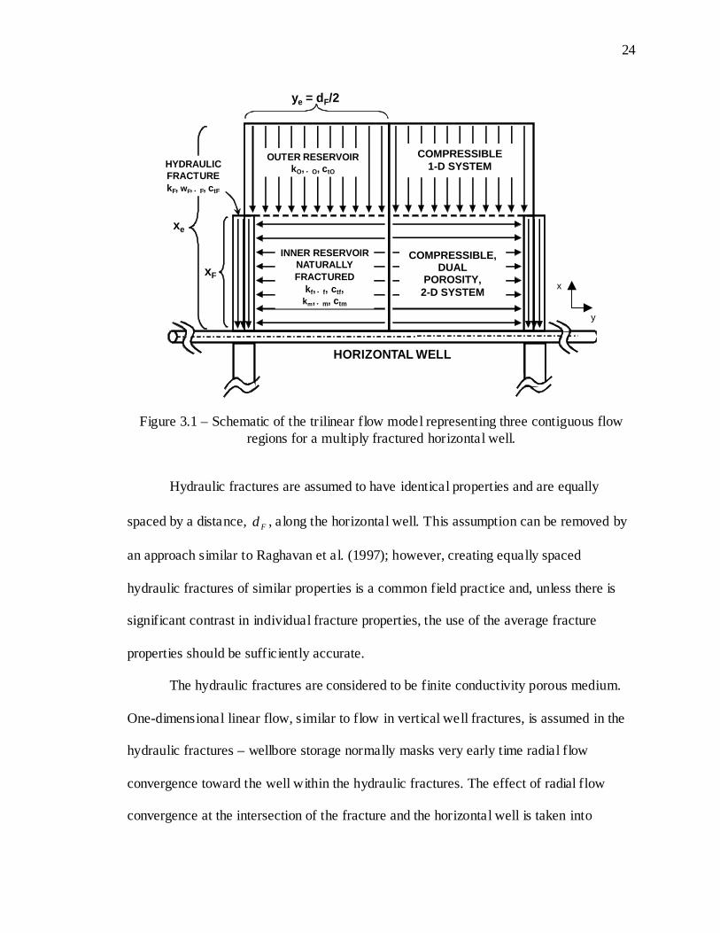
Figure 3.1 – Schematic of the trilinear flow model representing three contiguous flow

regions for a multiply fractured horizontal well.

Hydraulic fractures are assumed to have identical properties and are equally

spaced by a distance, Fd , along the horizontal well. This assumption can be removed by

an approach similar to Raghavan et al. (1997); however, creating equally spaced

hydraulic fractures of similar properties is a common field practice and, unless there is

significant contrast in individual fracture properties, the use of the average fracture

properties should be sufficiently accurate.

The hydraulic fractures are considered to be finite conductivity porous medium.

One-dimensional linear flow, similar to flow in vertical well fractures, is assumed in the

hydraulic fractures – wellbore storage normally masks very early time radial flow

convergence toward the well within the hydraulic fractures. The effect of radial flow

convergence at the intersection of the fracture and the horizontal well is taken into

xF

xe

ye = dF/2

OUTER RESERVOIRkO, . O, ctO

INNER RESERVOIRNATURALLYFRACTURED

kf, . f, ctf,km, . m, ctm

HYDRAULICFRACTUREkF, wF, . F, ctF

HORIZONTAL WELL

x

y

COMPRESSIBLE, DUAL

POROSITY, 2-D SYSTEM

COMPRESSIBLE 1-D SYSTEM

25

account, however, by a flow choking skin, discussed in Section 3.6. The wellbore storage

effect is incorporated into the model by convolution and is discussed in Section 3.7.

To simulate the performances of multiply fractured horizontal wells in shale, the

inner reservoir is allowed to be naturally fractured. A naturally fractured porous medium

is simulated through a dual porosity idealization using one of two common models –

either the pseudosteady model (Warren and Root, 1963) or the transient model (Kazemi,

1969, de Swaan-O, 1976, and Serra et al., 1983). The choice of the particular dual

porosity model does not affect the general solution for the trilinear flow model, presented

in Section 3.4, but does affect the definition of key parameters. The different dual

porosity models, and their definitions of key parameters, are discussed in detail in Section

3.5. A detailed discussion of flow regime characteristics of transient and pseudosteady

dual porosity models and their implications on pressure transient analysis is addressed in

Chapter 4.

Additionally, flow in the inner reservoir between the hydraulic fractures, and flow

in the outer reservoir beyond the tips of the hydraulic fractures, are both assumed to be

linear. Linear flow in the inner reservoir is a result of assuming either a non-perforated

horizontal well between the hydraulic fractures or assuming that the hydraulic fractures

dominate production. Due to the assumption of identical hydraulic fractures, the mid-line

between two fractures is a no-flow boundary.

For most common applications in shale reservoirs, the outer reservoir does not

contribute to production significantly. If it contributes however, its contribution at early

times is akin to linear flow toward a finite conductivity fracture. As discussed by

Raghavan et al. (1997) and Chen and Raghavan (1997), at long times, a multiply

26

fractured horizontal well behaves like a single fracture of length equal to the distance

between the two outermost fractures along the horizontal well. Therefore, flow

convergence from the outer reservoir is mainly in the direction perpendicular to flow

convergence in the inner reservoir. Unless the horizontal well is short, minimum

allowable flow rates are reached under this flow regime.

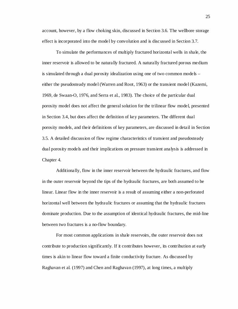
Under the conditions assumed here, the pressure transient response of a horizontal

well with Fn identical transverse hydraulic fractures can be modeled by considering only

one of the fractures producing from a rectangular reservoir section at a rate equal to

FF nqq = , where q is the total flow rate of the horizontal well. As sketched in Figs. 3.1

and 3.2, the fracture is located centrally in the closed rectangular drainage area. The no-

flow boundaries parallel to the fracture are located at the mid-line between the two

fractures, 2Fe dy = . The lateral boundaries perpendicular to the fracture plane are at a

distance ex from the center of the fracture. Therefore, the drainage area of the fracture is

equal to Fn1 of the total drainage area of the horizontal well. The fracture has a half-

length of Fx , a width of Fw , and penetrates the entire thickness, h , of the formation.

Figure 3.2 – Multiply fractured horizontal well and the symmetry element used in deriving the trilinear flow model.

27

The analytical expressions for the trilinear flow model are presented in Section

3.3, below. For discussion purposes, essential definitions are presented in Section 3.2,

immediately following.

3.2 Definitions

For convenience, the trilinear flow solution is derived in terms of consistent units

and dimensionless variables. Here, definitions of the dimensionless variables used in the

general form of the trilinear flow model are presented. The modifications necessary to

accommodate for a naturally fractured inner reservoir, gas flow, choking, and wellbore

storage are all presented in Sections 3.4 through 3.7, respectively.

Dimensionless pressure and time may be defined, respectively, by

( )ppqB

hkpqB

hkp iIIII

D −=∆=µ

πµ

π 22 , (3.5)

and

tx

tF

ID 2

η= , (3.6)

where

( ) µφ

ηIt

II c

k= . (3.7)

In Eqs 3.5, 3.6, and 3.7, and the rest of the definitions given here, the subscript I , refers

to the property of the inner reservoir. Dimensionless distances in the −x and −y

directions are respectively defined by

F

D xxx = (3.9)

28

and

F

D xyy = . (3.10)

The dimensionless distances to the reservoir boundaries are given by eDx and eDy . The

dimensionless width of the hydraulic fracture is given by

F

FD x

ww = . (3.11)

In the trilinear model, the following definitions of dimensionless fracture and reservoir

conductivities, respectively, are used:

FI

FFFD xk

wkC = (3.12)

and

eO

FIRD yk

xkC = . (3.13)

The following diffusivity ratios are also defined:

I

FFD η

ηη = (3.14)

and

I

OOD η

ηη = , (3.15)

where Iη is the diffusivity of the inner reservoir (Eq. 3.7) and Fη and Oη are the

diffusivities of the hydraulic fracture and outer reservoir given, respectively, by

( ) µφ

ηFt

FF c

k= (3.16)

and

29

( ) µφ

ηOt

OO c

k= . (3.17)

As a first approximation, for horizontal wells producing from shale, the outer

reservoir properties may be taken to be the same as those of the inner reservoir matrix.

3.3 Derivation of the Analytic Solution

In this section, the derivation of the general trilinear flow solution is presented.

The analytical derivation of the trilinear flow model follows the same lines as Cinco and

Meng (1988) who presented the finite conductivity fracture solution in a dual porosity

reservoir. Because of the symmetry of the system, it is sufficient to consider one-quarter

of a hydraulic fracture in a rectangular drainage region as shown in Figs. 3.1 and 3.2. The

solutions are derived for the outer reservoir, the inner reservoir, and the hydraulic

fracture, and then the solutions are coupled by using pressure continuity conditions on the

interfaces between the regions. It is more convenient to derive the solution in the Laplace

transform domain because the inner reservoir may be naturally fractured. In this work,

Stehfest’s algorithm (1970) is used to numerically invert the results into the time domain.

3.3.1 The Outer Reservoir Solution

The first step in the derivation of the trilinear flow solution is deriving the outer

reservoir solution starting from Eq. 3.3, previously presented:

t

pcpk O

tOOOO ∂∂

=∇ µφ2 , (3.18)

30

noting that the subscript O denotes parameters specific to the outer reservoir. Flow from

the outer reservoir to the inner reservoir is assumed to be linear, as shown in Fig. 3.1, and

therefore Eq. 3.18 may be rewritten in one dimension as follows:

t

pc

xp

k OtOO

OO ∂

∂=

∂∆∂

µφ2

2

. (3.19)

Converting Eq. 3.19 into dimensionless form, using the definitions from Section 3.2,

yields

012

2

=∂

∂−

∂∂

D

OD

ODD

OD

tp

xp

η. (3.20)

Applying the Laplace transformation to Eq. 3.20 and assuming that the initial

pressure, ip , is uniform in the entire system yields the following expression

02

2

=−∂

∂OD

ODD

OD psxp

η. (3.21)

The bar sign over the variables in Eq. 3.21 and hereafter indicates their Laplace transform

with respect to the time variable, Dt , and s is the Laplace transform parameter. The

general solution of Eq. 3.21 is given by

( ) ( )DODOOD xsBxsAp expexp +−= , (3.22)

where

OD

Oss

η= . (3.23)

The outer boundary of the outer reservoir is assumed to be a no-flow boundary.

This boundary condition should be appropriate to represent both the drainage boundary

between two parallel horizontal wells and impermeable physical boundaries. In most

practical cases, however, the effect of the outer boundary of the outer reservoir will not

31

be felt during the productive life of the well due to the length of time required for the

pressure pulse to reach the outer boundary of the reservoir through the tight matrix, as

will be demonstrated later in this work. The appropriate mathematical expression for the

no-flow outer boundary condition is given by

0=

∂∂

= eDD xxD

OD

xp . (3.24)

Taking the derivative of Eq. 3.22 and using the outer boundary condition results in

( ) ( ) 0expexp =+−−=

∂∂

=

eDOOeDOOxxD

OD xsBsxsAsxp

eDD

. (3.25)

Rearranging Eq. 3.25 and solving for B yields

( )eDO xsAB 2exp −= . (3.26)

Substituting Eq. 3.26 back into Eq. 3.22 and rearranging results in

( ) ( )[ ] ( )[ ]{ }DeDODeDOeDOOD xxsxxsxsAp −−+−−= expexpexp . (3.27)

At the inner boundary of the outer reservoir ( 1=Dx ), the pressures of the inner

and outer reservoirs must be equal; that is,

( ) ( ) 11 == =DD xIDxOD pp . (3.28)

Using Eqs. 3.27 and 3.28 results in

( ) ( ) ( )[ ] ( )[ ]{ } ( ) 11 1exp1expexp == =−−+−−=DD xIDeDOeDOeDOxOD pxsxsxsAp (3.29)

and subsequently solving Eq. 3.29 for A yields

( )

( ) ( )[ ] ( )[ ]{ }1exp1expexp1

−−+−−= =

eDOeDOeDO

xID

xsxsxs

pA D . (3.30)

Finally, substituting Eq. 3.30 back into 3.27 results in

32

( ) ( ) ( )( )( )( ) ( )

( )

( )

−

−

=−

−= ===

1cosh

cosh

1coshcosh

111

eDOD

DeDOD

xIDeDO

DeDOxIDxOD

xs

xxs

pxs

xxspp

DDD

η

η.(3.31)

Eq. 3.31 is the solution for the outer reservoir ready to be coupled with the inner

reservoir solution via the outer boundary condition for the inner reservoir (pressure

continuity at the boundary). Note that properties for the outer reservoir are carried in the

definition for ODη , Eq. 3.15.

3.3.2 The Inner Reservoir Solution

The second step in the derivation of the trilinear flow solution is deriving the

inner reservoir solution starting from Eq. 3.3, previously presented:

tp

cpk ItIIII ∂

∆∂=∇ µφ2 , (3.32)

noting that the subscript I denotes parameters specific to the inner reservoir. As shown in

Fig. 3.1, flow from the outer reservoir to the inner reservoir is assumed to be linear in the

x-direction, and flow from the inner reservoir to the hydraulic fracture is also assumed to

be linear – in the y-direction, however. Therefore Eq. 3.32 may be rewritten in two

dimensions as follows:

tp

kc

yp

xp I

I

tIIII

∂∆∂

=∂∆∂

+∂∆∂ µφ

2

2

2

2

. (3.33)

Integrating both sides of Eq. 3.33 as follows:

xtp

kc

xy

px

xp FFF x

I

I

tIIx

Ix

I ∂∂∆∂

=∂∂∆∂

+∂∂∆∂

∫∫∫00

2

2

02

2 µφ, and (3.34)

using the following pseudofunction assumptions:

33

( )xfy

pI ≠∂

∂ , and (3.35)

( )xft

pI ≠∂

∂ , (3.36)

results in

tp

kc

xp

xyp I

I

tIII

F

I

∂∆∂

=∂∆∂

+

∂∆∂ µφ1

2

2

. (3.37)

Recognizing the continuity of flux at the boundary of the inner and outer

reservoirs, as follows:

FF xx

OO

xx

II x

phk

xp

hk==

∂∆∂

=

∂∆∂

, (3.38)

Eq. 3.37 may be modified to

tp

kc

xp

xkk

yp I

I

tII

xx

O

FI

OI

F∂∆∂

=

∂∆∂

+

∂∆∂

=

µφ2

2

. (3.39)

Converting Eq. 3.39 into dimensionless form, using the definitions from Section 3.2, and

simplifying, yields

D

ID

xD

OD

FI

FO

D

ID

tp

xp

xkxk

yp

D∂∂

=

∂∂

+∂

∂

=12

2

. (3.40)

It is useful here, for analysis purposes, to define a dimensionless reservoir

conductivity, RDC , Eq. 3.13 (after Bennett et al. 1985), that relates flow in the inner

reservoir to flow in the outer reservoir. Dimensionless reservoir conductivity is akin to

hydraulic fracture conductivity as typically used in petroleum engineering. To

accomplish this, the horizontal length of the reservoir in the y-direction, ey , is included

in Eq. 3.40 as follows:

34

D

ID

xD

OD

e

e

FI

FO

D

ID

tp

xp

yy

xkxk

yp

D∂∂

=

∂∂

+

∂∂

=12

2

. (3.41)

Rearranging and simplifying the terms of Eq. 3.41 results in

01

12

2

=∂∂

−

∂∂

+

∂∂

= D

ID

xD

OD

eDRDD

ID

tp

xp

yCyp

D

. (3.42)

Applying the Laplace transformation to Eq. 3.42 yields the following expression

01

12

2

=−

+

=

IDxD

OD

eDRDD

ID pudxpd

yCdypd

D

, (3.43)

where the variable u has been introduced for notational convenience and su = for a

homogeneous reservoir. If a naturally fractured inner reservoir is to be considered, then

( )ssfu = and ( )sf is a dual porosity reservoir parameter defined by either the

pseudosteady state (Warren and Root, 1963) or transient (Kazemi, 1969, de Swaan-O,

1976, and Serra et al., 1983) models – discussed in greater detail in Section 3.4. The

derivation of Eq. 3.43 for dual porosity idealization is standard and can be found in the

fundamental literature of dual porosity models (Warren and Root, 1963, Kazemi, 1969,

de Swaan-O, 1976, and Serra et al., 1983). An important point to note here is that the dual

porosity idealization assumes negligible fluid transfer from the matrix to the well.

Therefore, Eq. 3.43 for dual porosity reservoirs is expressed in terms of the pressure in

the natural fractures ( fDID pp = ) and the permeability used in the definitions of

dimensionless variables is the permeability of the natural fractures ( fI kk = ).

Furthermore, fI kk = is defined as a bulk property for the pseudosteady dual porosity

model and as an intrinsic one for the transient dual porosity model. Similarly, the

thickness used in the equations and definitions of dimensionless variables is the total

35

system thickness for the pseudosteady model and the total fracture thickness for the

transient model. Finally, the diffusivity constant of the inner reservoir, Iη , is defined

based on the bulk compressibility-storativity product of the total system (matrix and

natural fractures) for the pseudosteady dual porosity model and the intrinsic

compressibility-storativity product of the natural fractures for the transient dual porosity

model. These definitions will be provided in Section 3.4.

Recalling that the outer reservoir solution, Eq. 3.31, relates the pressures of the

inner and outer reservoirs at their mutual boundary, the ODp term in Eq. 3.43 can be

expressed in terms of IDp . Then, taking the derivative of the outer reservoir solution, Eq.

3.31, as follows:

( )( )

( )

−

−

−=

=

1cosh

sinh

1

eDOD

DeDOD

ODxID

D

OD

xs

xxssp

dxpd

D

η

ηη , (3.44)

yields at the interface of the inner and outer reservoirs ( 1=Dx )

( ) ( )

−−=

=

=

1tanh11

eDODOD

xIDxD

OD xsspdxpd

D

D

ηη . (3.45)

Then, defining

( )

−= 1tanh eD

ODODO xss

ηηβ (3.46)

results in

( ) 11

==

−=

D

D

xIDOxD

OD pdxpd

β . (3.47)

Equation 3.47 may be substituted back into Eq. 3.43 to obtain

36

( ) 012

2

=−− = IDxIDeDRD

O

D

ID pupyCdy

pdD

β . (3.48)

Using the pseudofunction assumption to state that pressure of the inner reservoir is not a

function of distance in the x-direction, or ( )DID xfp ≠ , Eq. 3.48 may be simplified to

02

2

=

+− u

yCp

dypd

eDRD

OID

D

ID β . (3.49)

Defining

uyC eDRD

OO +=

βα (3.50)

allows for Eq. 3.49 to be further simplified to yield

02

2

=− IDOD

ID pdy

pdα . (3.51)

Then, the general solution of Eq. 3.51 is given by

( ) ( )DODOID yByAp αα expexp +−= . (3.52)

Due to the symmetry of the system, there is a no-flow boundary created in

between the hydraulic fractures, as seen in Fig. 3.1. This no-flow boundary forms the

outer boundary of the inner reservoir. The mathematical expression of the outer boundary

condition for the inner reservoir solution is

0=

= eDD yyD

ID

dypd . (3.53)

Taking the derivative of Eq. 3.52 and using the outer boundary condition, Eq. 3.52,

results in

( ) ( ) 0expexp =+−−=

=

eDOOeDOOyyD

ID yByAdypd

eDD

αααα . (3.54)

37

Rearranging Eq. 3.54 and solving for B yields

( )eDO yAB α2exp −= . (3.55)

Substituting Eq. 3.55 back into Eq. 3.52, and rearranging, results in

( ) ( )[ ] ( )[ ]{ }DeDODeDOeDOID yyyyyAp −−+−−= ααα expexpexp . (3.56)

At the inner boundary of the inner reservoir, where the pressure of the hydraulic

fracture and the inner reservoir must be equal, the condition may be expressed as

( ) ( ) 22 DDDD wyFDwyID pp == = . (3.57)

Note that the inner boundary of the inner reservoir is equal to 2Dw , or half of the total

fracture width as measured from the mid-line of the fracture, in dimensionless form, due

to the geometry of the problem and the dimensionless variable definition set forth in

Section 3.2. Substituting Eq. 3.56 into the inner boundary condition, Eq. 3.57, results in

( ) ( )

( )[ ] ( )[ ]{ } ( ) 222

2

expexp

exp

DD

DD

DD

wyFDw

eDOw

eDO

eDOwyID

pyy

yAp

=

=

=−−+−×

×−=

αα

α (3.58)

and subsequently using Eq. 3.58 to solve for A yields

( )

( ) ( )[ ] ( )[ ]{ }22

2

expexpexp DD

DD

weDO

weDOeDO

wyFD

yyy

pA

−−+−−= =

ααα. (3.59)

Finally, substituting Eq. 3.59 back into 3.56, simplifying, and reorganizing yields

( ) ( ) ( )( )( )( )2

22 coshcosh

DDDDD weDO

DeDOwyFDwyID y

yypp

−

−= == α

α. (3.60)

Eq. 3.60 is the solution for the inner reservoir ready to be coupled with the

hydraulic fracture solution via the outer boundary condition for the hydraulic fracture

(pressure continuity at the boundary). Note that properties for both the inner and outer

reservoirs are carried in the definition for Oα , Eq. 3.50.

38

3.3.3 The Hydraulic Fracture Solution

The third step in the derivation of the trilinear flow solution is deriving the

hydraulic fracture solution starting from Eq. 3.3, previously presented:

tpcpk F

tFFFF ∂∆∂

=∇ µφ2 , (3.61)

noting that the subscript F denotes parameters specific to the hydraulic fracture. As

shown in Fig. 3.1, flow from the inner reservoir to the hydraulic fracture is assumed to be

linear in the y-direction, and flow from the hydraulic fracture to the wellbore is also

assumed to be linear – in the x-direction, however. Therefore Eq. 3.61 may be re-written

in two dimensions as follows:

tp

kc

yp

xp F

F

tFFFF

∂∆∂

=∂∆∂

+∂∆∂ µφ

2

2

2

2

. (3.62)

Integrating both side of Eq. 3.62 as follows:

ytp

kc

yypy

xp

FwFwFw

F

F

tFFFF ∂∂∆∂

=∂∂∆∂

+∂∂∆∂

∫∫∫222

002

2

02

2 µφ , and (3.63)

using the following pseudofunction assumptions:

( )yfx

pF ≠∂

∂ , and (3.64)

( )yft

pF ≠∂

∂ , (3.65)

results in

tp

kc

yp

wxp F

F

tFF

y

F

F

F

Fw ∂∆∂

=

∂∆∂

+∂∆∂

=

µφ

2

22

2

. (3.66)

39

Recognizing the continuity of flux at the boundary of the hydraulic fracture and

the inner reservoir, as follows:

22

FF wy

II

wy

FF y

phkyphk

==

∂∆∂

=

∂∆∂ , (3.67)

Eq. 3.66 may be modified to yield

tp

kc

yp

kk

wxp F

F

tFF

y

I

F

I

F

F

Fw ∂∆∂

=

∂∆∂

+∂∆∂

=

µφ

2

22

2

. (3.68)

Converting Eq. 3.68 into dimensionless form, using the definitions from Section 3.2, and

simplifying, yields

D

FD

FtII

ItFF

wyD

ID

FF

FI

D

FD

tp

kckc

yp

wkxk

xp

DD

∂∂

=

∂∂

+∂

∂

=µφµφ

2

2

2 2 . (3.69)

Including the definitions for FDC and FDη , given respectively by Eqs. 3.12 and 3.14,

results in

D

FD

FDwyD

ID

FDD

FD

tp

yp

Cxp

DD

∂∂

=

∂∂

+∂

∂

=η

12

2

2

2

. (3.70)

Applying the Laplace transformation to Eq. 3.70 yields the following expression

02

2

2

2

=−

+

=

FDFDwyD

ID

FDD

FD psdypd

Cdxpd

DD

η. (3.71)

Recalling that the inner reservoir solution relates the pressures of the hydraulic fracture

and the inner reservoir at their mutual boundary, and taking the derivative of the inner

reservoir solution, Eq. 3.60, as follows:

( ) ( )( )( )( )2

2 coshsinh

DD

D weDO

DeDOOwyFD

D

ID

yyy

pdypd

−

−−=

= α

αα , (3.72)

40

yields

( ) ( )[ ]22

2

tanh DD

DD

D

weDOOwyFD

wyD

ID ypdypd

−−=

=

=

αα , (3.73)

Then, defining

( )[ ]2tanh DweDOOF y −= ααβ (3.74)

results in

( )2

2

DD

DD

wyFDFwyD

ID pdypd

==

−=

β . (3.75)

Equation 3.75 may be substituted back into Eq. 3.71, resulting in

( ) 0222

2

=−− = FDFD

wyFDFD

F

D

FD pspCdx

pdD

D ηβ . (3.76)

Using the pseudofunction assumption to state that the pressure of the hydraulic fracture is

not a function of the distance in the y-direction, or ( )DFD yfp ≠ , Eq. 3.76 may be

simplified to

022

2

=

−−

FDFD

FFD

D

FD sC

pdx

pdη

β . (3.77)

Defining

FDFD

FF

sC η

βα +=

2 (3.78)

allows for Eq. 3.77 to be further simplified, yielding

02

2

=− FDFD

FD pdx

pdα . (3.79)

Then, the general solution of Eq. 3.79 is given by

( ) ( )DFDFFD xBxAp αα expexp +−= . (3.80)

41

The outer boundary of the hydraulic fracture is the tip of the fracture. Assuming

there is no flow across the fracture tip, the outer boundary condition for purposes of the

hydraulic fracture solution is then

01

=

=DxD

FD

dxpd . (3.81)

Taking the derivative of Eq. 3.80 and using in the outer boundary condition, Eq. 3.81,

results in

( ) ( ) 0expexp1

=+−−==

FFFFxD

FD BAdxpd

D

αααα . (3.82)

Rearranging Eq. 3.82 and solving for A yields

( )FBA α2exp= . (3.83)

Substituting Eq. 3.83 back into Eq. 3.80, and rearranging, results in

( )[ ] ( )DFDFFD xBxBp αα exp2exp +−= . (3.84)

The coefficient B in Eq. 3.84, can be determined from an inner boundary

condition for the fracture. To develop the inner boundary condition for the hydraulic

fracture solution, flow from the hydraulic fracture to the wellbore must be considered.

Starting with Darcy’s Law:

FF p

kv ∇=

µ, (3.85)

where v is the fluid velocity, Fk is the permeability of the hydraulic fracture, µ is the

fluid viscosity, and Fp is the pressure in the hydraulic fracture, and, as shown in Fig. 3.1,

considering linear flow from the hydraulic fracture into the wellbore in the x-direction,

volumetric velocity crossing the wellbore surface in the fracture is given by:

42

0=

∂∆∂

−=x

FFx x

pkvµ

. (3.86)

Note that the wellbore surface, the inner boundary of the hydraulic fracture, is

represented by a rectangular plane at 1=Dx , having dimensions equal to the width and

height of the fracture. Flow rate passing through the wellbore surface can be computed by

evaluating the surface integral of Eq. 3.86, as follows:

∫ ∫∫ ∫ ∂∂

∂∆∂

−=∂∂=

2 22 2

0 0 00 0

Fw hFw h

yzxpkyzv

x

FFx µ

. (3.87)

Because the total flow rate crossing the wellbore surface is the sum of the fluxes coming

from both sides of the rectangular plane representing the wellbore and only one-quarter

of the fracture is modeled, due to the symmetry, Eq. 3.87 may be related to the fracture

flow rate, Fq , as follows

0228 =

∂∆∂

−=x

FFFF

xphwkq

µ. (3.88)

In Eq. 3.88, individual fracture flow rate Fq is related to the multiply fractured horizontal

well flow rate q by the relation FF nqq = because of the assumption of uniform

distribution of Fn identical fractures along the horizontal well under linear flow.

Converting Eq. 3.88 into dimensionless form, using the definitions from Section 3.2, and

simplifying, yields

0

1=

∂∂

−=DxD

FD

FI

FF

xp

xkBwk

π. (3.89)

Recalling the definition of FDC given in Eq. 3.12, Eq. 3.89 may be restated as follows:

43

FDxD

FD

Cxp

D

π−=

∂∂

=0

. (3.90)

Applying the Laplace transformation to Eq. 3.90 results in the following expression:

FDxD

FD

sCdxpd

D

π−=

=0

. (3.91)

Equation 3.91 is the inner boundary condition used in the hydraulic fracture solution.

Substituting Eq. 3.84 into Eq. 3.91 yields

( )FD

FFFxD

FD

sCBB

dxpd

D

πααα −=+−=

=

2exp0

. (3.92)

Subsequently solving Eq. 3.92 for B results in

( )[ ]FFFDsCB

ααπ

2exp1−−= . (3.93)

Finally, substituting Eq. 3.93 back into 3.84, simplifying, and recognizing the definition

of tangent hyperbolic from the resulting identity, yields

( )[ ]

( )F

DF

FFDFD

xsC

pα

αα

πsinh

1cosh −= . (3.94)

Equation 3.94 is the solution for the pressure distribution in the hydraulic fracture.

Because of the pressure continuity at the interface between the hydraulic fracture and the

wellbore, dimensionless wellbore pressure is readily written from Eq. 3.94 as follows:

( ) ( )FFFDxFDwD sC

ppD αα

πtanh0 == = . (3.95)

The dimensionless wellbore pressure solution given in Eq. 3.95 constitutes the

fundamental contribution of this thesis, the trilinear model, which couples the outer

reservoir, the inner reservoir, and the hydraulic fracture together. Note that properties for

44

both the inner and outer reservoirs, as well as the hydraulic fracture, are carried in the

definition for Fα , Eq. 3.78. In the Section 3.4, following, modifications to Eq. 3.95

necessary to accommodate a naturally fractured, dual porosity, inner reservoir will be

discussed. Subsequent sections will also address modifications necessary for the

treatment of gas flow, choking effects, and wellbore storage.

3.4 Dual Porosity Parameters

Section 3.3 above presents an analytic solution for a hydraulically fractured

horizontal well in a shale formation. Practically, the act of hydraulically fracturing tight

media like shale may frequently reactivate any existing natural fracture network or create

a new network of small induced fractures that behave like a natural fracture network. For

this reason, the trilinear model presented in Eq. 3.95 above is more practically applicable

when it accounts for the presence of fractured media in the system, whether that media

was naturally fractured or the fractures were induced. For convenience, both types of

fracture systems are referred to as a ‘natural fracture network’ in this thesis. For the

system described here, it is the inner reservoir that may be naturally fractured.

Recall that Eq. 3.43, in the development of the inner reservoir solution, contained

a parameter u , which, for dual-porosity media, was defined as

( )ssfu = . (3.96)

This term allows for the inclusion of parameters for a naturally fractured inner reservoir.

The function ( )sf varies according whether the inner reservoir is homogeneous or

naturally fractured, and if naturally fractured, which of the two common dual porosity

models is used to characterize the media. The pseudosteady model considers

45

pseudosteady fluid transfer from the matrix to the fracture (Warren and Root, 1963). The

model that incorporates transient fluid transfer from the matrix to the fracture (Kazemi,

1969, de Swaan-O, 1976, Serra et al., 1983) is referred to as the transient model. The

choice of the particular dual porosity model does not affect the general solution for the

trilinear flow model, but does affect the definition of key parameters. For a homogeneous

inner reservoir,

( ) 1=sf . (3.97)

For a naturally fractured, dual porosity, inner reservoir, using the pseudosteady model,

( )( ) λω

λωω+−+−

=11)(

sssf and (3.98)

using the transient model,

( )λωωλˆˆ3tanh

3ˆˆ

1 ss

sf += . (3.99)

In dual porosity idealizations, a naturally fractured reservoir may be characterized

in terms of either intrinsic or bulk properties. If ζχ denotes an intrinsic property of the

medium m=ζ (matrix) or f (fracture), then the bulk properties of the medium ζ are

defined by

ξξξ χχ r=~ , (3.100)

where bVVr ξξ = or the ratio of the volume of the medium ζ , ζV , to the bulk volume of

the system, bV . It is customary to introduce the pseudosteady dual porosity model

(Warren and Root, 1963) in terms of bulk properties. Characteristics of the matrix and

fracture media are incorporated into the pseudosteady dual porosity medium by the

storativity and transmissivity ratios defined by

46

( )

( ) ( )mtft

ft

cc

c~~~~

~~

φφ

φω

+= , (3.101)

and

f

m

kk~~

2σλ = , (3.102)

respectively.

In Eq. 3.102, is a reference length used consistently in the definition of

dimensionless variables. In this thesis, the reference length is the hydraulic fracture

half-length; that is, Fx= . In comparing the results of this study with other models,

adjustments should be made to the values of λ to compensate for different choices in

reference length.

The definition of the matrix shape factor, σ , in Eq. 3.102 is an important issue,

but the discussion is outside the scope of this thesis. Kazemi et al. (1976) proposed the

following first approximation for the shape factor of rectangular matrix blocks of

dimension zyx LLL ×× :

++=

222

1114zyx LLL

σ . (3.103)

Square matrix blocks of size L are employed here and 212 L=σ is used to compute the

shape factor. Note that choosing the matrix slab thickness, mth , for the transient model

such that it is equal to the size of the square matrix blocks, L , for the pseudosteady

model, yields the same value of the transmissivity ratio, λ or λ̂ , for both models.

The transient dual porosity model (Kazemi, 1969, de Swaan-O, 1976, and Serra et

al., 1983) may be introduced in terms of either intrinsic or bulk properties of the fracture

47

and matrix media. Here, the Serra et al. (1983) derivation of the transient dual porosity

model in terms of intrinsic properties is followed. This model represents the naturally

fractured reservoir as a stack of alternating matrix and fracture slabs. If fh and mh denote

the thickness of each fracture and matrix slab, respectively, and fn and mn are the number

of fracture and matrix slabs, respectively, then the total thicknesses of fracture and matrix

slabs, respectively, are ffft hnh = and mmmt hnh = . Thus, the formation thickness is

mtftI hhh +=

. For the transient dual porosity model, Serra et al. (1983) define the

storativity and transmissivity ratios by

( )( ) ft

mt

cc

φφ

ω =ˆ , (3.104)

and

=

=

ff

mm

mftf

mtm

m hkhk

hhkhk

h 2

2

2

2

1212ˆ λ (3.105)

respectively.

As mentioned in Section 3.2, if a naturally fractured inner reservoir is modeled,

then the permeability of the inner reservoir is the bulk permeability of the natural

fractures, fI kk ~

= , for the pseudosteady model and the intrinsic permeability of the

natural fractures, fI kk =

mtftI hhh +=

, for the transient model. Similarly, the thickness used in the

equations and definitions of dimensionless variables is the total system thickness,

, for the pseudosteady model and the total fracture thickness, ftI hh = , for

the transient model. Finally, the diffusivity constant of the inner reservoir is defined

48

based on the bulk compressibility-porosity product of the total system for the

pseudosteady model,

( ) ( ) ( )[ ] f

ftmt

f

It

II cc

kck η

µφφµφη ~

~~~~~

=+

== , (3.106)

and the intrinsic compressibility-porosity product of the natural fractures for the transient

model,

( ) ( ) fft

f

It

II c

kck η

µφµφη === . (3.107)

Due to the expectation of elongated transient flow periods in tight matrices, the

transient dual porosity model is preferred for the system discussed in this thesis. This

expectation is supported by the quarter slope behavior of the log-log pressure responses

of pressure transient tests observed in the field, which is a result of the intermediate time

behavior of the transient fluid transfer model.

A detailed discussion of the flow regime characteristics observed in transient and

pseudosteady dual porosity models, and their implications on pressure transient analysis,

occurs in Chapter 4. Here, it should be noted that the pseudosteady fluid transfer model

may be applicable in formations with matrix permeabilities much higher than those

observed in common applications of multiply fractured horizontal wells in shale.

3.5 Gas

The system for which the trilinear flow model was developed, namely a

hydraulically fractured horizontal well in a tight shale matrix, most commonly produces

gas. For ease of presentation, the analytic solution presented in Section 3.3 was

developed assuming liquid flow. Here, the modifications to the analytic solution of

49

Section 3.3 that are necessary to accommodate gas flow are presented. The modifications

are relatively straightforward, requiring only changes in dimensionless variable

definitions, originally set forth in Section 3.2, as follows

( )

( ) ( )[ ]

−

−=

gas,for 1422

and oil,for 2.141

pmpmqT

hk

ppqBhk

pi

II

iII

Dµ (3.108)

where ( )pm is the real gas pseudopressure defined by

( ) ∫ ′′

=p

pb

pdz

ppmµ

2 (3.109)

and

tx

tF

ID 2

η= , (3.110)

where

( ) µφ

ηIt

II c

k= . (3.111)

As an approximation for gas flow, the dimensionless time in Eq 3.110 may be

evaluated by using the values for Iη observed at the highest pressure during the test. The

hydraulic fracture and outer reservoir diffusivities, Fη and Oη , Eqs. 3.16 and 3.17,

respectively, may also be evaluated by using the values observed at the highest pressure

during the test.

3.6 Choking

Section 3.1 discussed several assumptions made to facilitate the development of

the analytical trilinear flow model. One of these was the assumption of one-dimensional

50

linear flow within the hydraulic fracture; that is, radial convergence of flow toward the

wellbore within the hydraulic fracture was ignored. To approximate radial convergence

of flow, Mukherjee and Economides (1991) provided the following equation to compute

a skin factor due to flow choking within the fracture:

−

=

22ln π

wFF

IIc r

hwkhk

s . (3.112)

Adding the choking skin to Eq. 3.95, the following solution is obtained, which is a

good approximation for dimensionless wellbore pressure after the end of radial flow in

the hydraulic fracture:

( ) ss

sCp c

FDwD +=

ααπtanh

. (3.113)

3.7 Wellbore Storage

To develop a more practical solution for pressure transient analysis purposes, the

effect of wellbore storage should be taken into account at early times. The effect of

wellbore storage can be incorporated into the solution by substituting wDp from Eq.

3.113 into the following expression:

wDD

wDstoragewD psC

pp 2, 1 +

= , (3.114)

where the dimensionless wellbore storage coefficient is given by

( ) 22615.5

FID xch

CCφπ

= . (3.115)

The definition of DC depends on the dual porosity model selected to represent the

inner reservoir. The porosity-compressibility product in the denominator of the right-

51

hand side of Eq. 3.115 refers to bulk properties of the total system,

( ) ( ) ( )ftmtIt ccc ~~~~ φφφ += , for the pseudosteady model and to the fracture medium,

( ) ( ) ftIt cc φφ = , for the transient model. Similarly, the thickness used in the equations and

definitions of dimensionless variables is the total system thickness, mtftI hhh += , for the

pseudosteady model and the total fracture thickness, ftI hh = , for the transient model.

Therefore, for the same value of wellbore storage coefficient, a different dimensionless

wellbore storage coefficient may be obtained for pseudosteady and transient dual porosity

models.

The solution given by Eq. 3.113 or 3.114 may also be used to compute

dimensionless buildup pressures from the following superposition equation:

( ){ } ( ){ } ( ){ } ( ){ }DwDDpDwDpDwDDsD tpLttpLtpLtpL ∆+∆+−=∆ , (3.116)

where

( )

( ) ( )[ ]

−

−=

gasfor 1422

oilfor 2.141

,

,

swfwsII

swfwsII

sD

pmpmqT

hk

ppqBhk

p µ . (3.117)

In Eq. 3.116, pDt is the dimensionless producing time, Dt∆ is the dimensionless

shut in time, and ( ){ }DD tpL denotes the Laplace transform of ( )DD tp with respect to Dt .

In Eq. 3.117, wsp is the bottom hole shut in pressure and swfp , is the bottom hole pressure

at the instant of shut-in.

52

CHAPTER 4

MODEL VERIFICATION

In this chapter, the new trilinear model is verified against a previously published

semianalytical model (Medeiros et al. , 2008) for the system addressed in this thesis – a

multiply fractured horizontal well in a shale formation. In the process of conducting this

verification, difficulties were encountered in reconciling the two different models for dual

porosity behavior – the pseudosteady model (Warren and Root, 1963) used by the

semianalytical solution and the transient dual porosity model (Kazemi, 1969, de Swaan-

O, 1976, Serra et al., 1983) that may be used in the trilinear analytical solution. As a

result, Section 4.2 is devoted to a discussion on the ramifications in the choice of dual

porosity model.

One of the advantages of the trilinear flow solution is its convenience in deriving

asymptotic approximations, and several are presented in Section 4.3. Though linear and

bilinear flow regimes have been noted for fractured horizontal wells in the literature

based on their diagnostic features, they have not been associated with particular reservoir

characteristics and flow relationships. The solutions documented in this work provide

insight about potential flow regimes and the conditions leading to these flow regimes.

Identification of these flow regimes is important for the characterization of shale

reservoirs from pressure transient tests. Because of its relative simplicity, the trilinear

model does not require special expertise to compute and apply.

53

A field example demonstrates the versatility of the solution in investigating the

effects of various parameters influencing pressure transient responses.

4.1 Model Verification

Chen and Raghavan (1997) and Raghavan et al. (1997) developed analytical

pressure transient solutions for multiply fractured horizontal wells in homogeneous

reservoirs by using the ideas of Bennett et al. (1985) and Camacho et al. (1987) who

developed solutions for fractured vertical wells in layered reservoirs. For a homogenous

reservoir [ ( ) 1=sf and su = in Eq. 3.43], the trilinear flow model yields the same

asymptotic solutions at early times as Chen and Raghavan (1997) and Raghavan et al.

(1997). This provides analytical verification of the trilinear model.

The trilinear model is also verified by comparing the results with the

semianalytical solution of Medeiros et al. (2008). The semianalytical solution models

hydraulic fractures as porous media and considers radial flow convergence toward the

wellbore within the hydraulic fractures. Therefore, the semianalytical solution is expected

to capture the characteristics of the early-time flow regimes in hydraulic fractures

(fracture radial and radial-linear flow regimes). However, the accuracy of the

computations at very early times is hindered by the discretization of the boundaries.

Similarly, the trilinear flow model incorporates the effect of flow choking in hydraulic

fractures through a skin factor, and thus, becomes accurate after the end of early-time

radial flow in hydraulic fractures. Considering the limitations of the trilinear and

semianalytical models, differences are expected in the results of the two models at early

times. However, when the effect of wellbore storage is taken into account, the early-time

54

flow regimes are masked and the limitations of the models at early times become

insignificant for practical purposes. A comparison of results from the trilinear and

semianalytical models, without the effect of wellbore storage, is presented below. Then,

the effect of wellbore storage on early-time results is demonstrated. Table 4.1 presents

the data used for the comparison case. For convenience, input for well, reservoir, and

fluid properties, and the corresponding model input data, are documented. Inspection of

Table 4.1 should reveal the details of the physical system that can be considered with the

trilinear model.

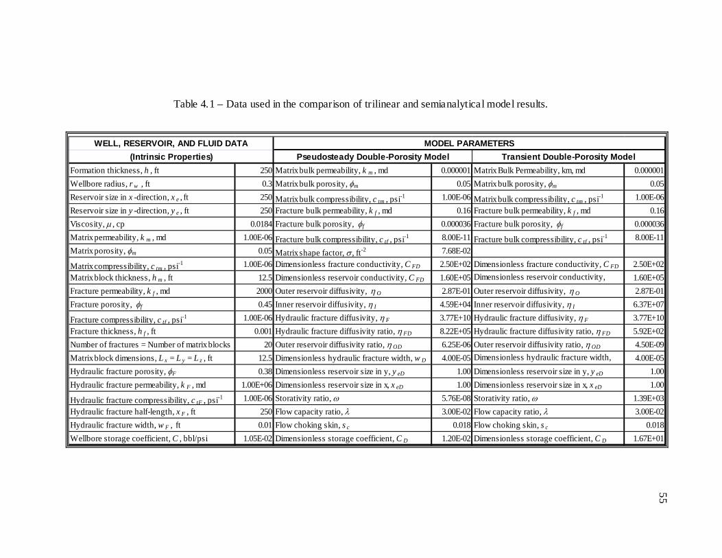
55

Table 4.1 – Data used in the comparison of trilinear and semianalytical model results.

Formation thickness, h , ft 250 Matrix bulk permeability, k m , md 0.000001 Matrix Bulk Permeability, km, md 0.000001Wellbore radius, r w , ft 0.3 Matrix bulk porosity, φm 0.05 Matrix bulk porosity, φm 0.05Reservoir size in x -direction, x e , ft 250 Matrix bulk compressibility, c tm , psi-1 1.00E-06 Matrix bulk compressibility, c tm , psi-1 1.00E-06Reservoir size in y -direction, y e , ft 250 Fracture bulk permeability, k f , md 0.16 Fracture bulk permeability, k f , md 0.16Viscosity, µ , cp 0.0184 Fracture bulk porosity, φf 0.000036 Fracture bulk porosity, φf 0.000036Matrix permeability, k m , md 1.00E-06 Fracture bulk compressibility, c tf , psi-1 8.00E-11 Fracture bulk compressibility, c tf , psi-1 8.00E-11Matrix porosity, φm 0.05 Matrix shape factor, σ , ft-2 7.68E-02

Matrix compressibility, c tm , psi-1 1.00E-06 Dimensionless fracture conductivity, C FD 2.50E+02 Dimensionless fracture conductivity, C FD 2.50E+02Matrix block thickness, h m , ft 12.5 Dimensionless reservoir conductivity, C FD 1.60E+05 Dimensionless reservoir conductivity, 1.60E+05Fracture permeability, k f , md 2000 Outer reservoir diffusivity, η O 2.87E-01 Outer reservoir diffusivity, η O 2.87E-01Fracture porosity, φf 0.45 Inner reservoir diffusivity, η I 4.59E+04 Inner reservoir diffusivity, η I 6.37E+07

Fracture compressibility, c tf , psi-1 1.00E-06 Hydraulic fracture diffusivity, η F 3.77E+10 Hydraulic fracture diffusivity, η F 3.77E+10Fracture thickness, h f , ft 0.001 Hydraulic fracture diffusivity ratio, η FD 8.22E+05 Hydraulic fracture diffusivity ratio, η FD 5.92E+02Number of fractures = Number of matrix blocks 20 Outer reservoir diffusivity ratio, η OD 6.25E-06 Outer reservoir diffusivity ratio, η OD 4.50E-09Matrix block dimensions, L x = L y = L z , ft 12.5 Dimensionless hydraulic fracture width, w D 4.00E-05 Dimensionless hydraulic fracture width, 4.00E-05Hydraulic fracture porosity, φF 0.38 Dimensionless reservoir size in y, y eD 1.00 Dimensionless reservoir size in y, y eD 1.00Hydraulic fracture permeability, k F , md 1.00E+06 Dimensionless reservoir size in x, x eD 1.00 Dimensionless reservoir size in x, x eD 1.00

Hydraulic fracture compressibility, c tF , psi-1 1.00E-06 Storativity ratio, ω 5.76E-08 Storativity ratio, ω 1.39E+03Hydraulic fracture half-length, x F , ft 250 Flow capacity ratio, λ 3.00E-02 Flow capacity ratio, λ 3.00E-02Hydraulic fracture width, w F , ft 0.01 Flow choking skin, s c 0.018 Flow choking skin, s c 0.018Wellbore storage coefficient, C , bbl/psi 1.05E-02 Dimensionless storage coefficient, C D 1.20E-02 Dimensionless storage coefficient, C D 1.67E+01

WELL, RESERVOIR, AND FLUID DATA MODEL PARAMETERS(Intrinsic Properties) Pseudosteady Double-Porosity Model Transient Double-Porosity Model

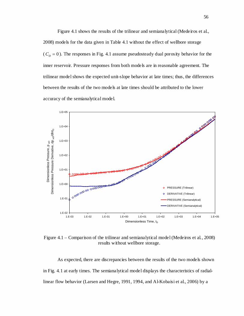
56

56

Figure 4.1 shows the results of the trilinear and semianalytical (Medeiros et al.,

2008) models for the data given in Table 4.1 without the effect of wellbore storage

( 0=DC ). The responses in Fig. 4.1 assume pseudosteady dual porosity behavior for the

inner reservoir. Pressure responses from both models are in reasonable agreement. The

trilinear model shows the expected unit-slope behavior at late times; thus, the differences

between the results of the two models at late times should be attributed to the lower

accuracy of the semianalytical model.

1.E-02

1.E-01

1.E+00

1.E+01

1.E+02

1.E+03

1.E+04

1.E+05

1.E-03 1.E-02 1.E-01 1.E+00 1.E+01 1.E+02 1.E+03 1.E+04 1.E+05

Dimensionless Time, tD

Dim

ensi

onle

ss P

ress

ure,

p w

D

Dim

ensi

onle

ss P

ress

ure

Der

ivat

ive,

dp

wD/d

lnt D

PRESSURE (Trilinear)

DERIVATIVE (Trilinear)

PRESSURE (Semianalytical)

DERIVATIVE (Semianalytical)

Figure 4.1 – Comparison of the trilinear and semianalytical model (Medeiros et al. , 2008) results without wellbore storage.

As expected, there are discrepancies between the results of the two models shown

in Fig. 4.1 at early times. The semianalytical model displays the characteristics of radial-

linear flow behavior (Larsen and Hegre, 1991, 1994, and Al-Kobaisi et al., 2006) by a

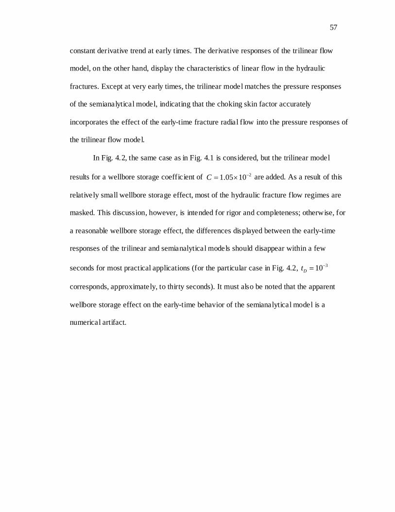
57

57

constant derivative trend at early times. The derivative responses of the trilinear flow

model, on the other hand, display the characteristics of linear flow in the hydraulic

fractures. Except at very early times, the trilinear model matches the pressure responses

of the semianalytical model, indicating that the choking skin factor accurately

incorporates the effect of the early-time fracture radial flow into the pressure responses of

the trilinear flow model.

In Fig. 4.2, the same case as in Fig. 4.1 is considered, but the trilinear model

results for a wellbore storage coefficient of 21005.1 −×=C are added. As a result of this

relatively small wellbore storage effect, most of the hydraulic fracture flow regimes are

masked. This discussion, however, is intended for rigor and completeness; otherwise, for

a reasonable wellbore storage effect, the differences displayed between the early-time

responses of the trilinear and semianalytical models should disappear within a few

seconds for most practical applications (for the particular case in Fig. 4.2, 310−=Dt

corresponds, approximately, to thirty seconds). It must also be noted that the apparent

wellbore storage effect on the early-time behavior of the semianalytical model is a

numerical artifact.

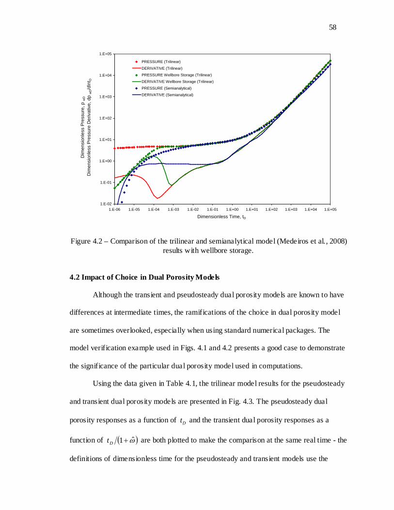
58

58

1.E-02

1.E-01

1.E+00

1.E+01

1.E+02

1.E+03

1.E+04

1.E+05

1.E-06 1.E-05 1.E-04 1.E-03 1.E-02 1.E-01 1.E+00 1.E+01 1.E+02 1.E+03 1.E+04 1.E+05

Dimensionless Time, tD

Dim

ensi

onle

ss P

ress

ure,

p w

D

Dim

ensi

onle

ss P

ress

ure

Der

ivat

ive,

dp

wD/d

lnt D

PRESSURE (Trilinear)

DERIVATIVE (Trilinear)

PRESSURE Wellbore Storage (Trilinear)

DERIVATIVE Wellbore Storage (Trilinear)

PRESSURE (Semianalytical)

DERIVATIVE (Semianalytical)

Figure 4.2 – Comparison of the trilinear and semianalytical model (Medeiros et al. , 2008) results with wellbore storage.

4.2 Impact of Choice in Dual Porosity Models

Although the transient and pseudosteady dual porosity models are known to have

differences at intermediate times, the ramifications of the choice in dual porosity model

are sometimes overlooked, especially when using standard numerical packages. The

model verification example used in Figs. 4.1 and 4.2 presents a good case to demonstrate

the significance of the particular dual porosity model used in computations.

Using the data given in Table 4.1, the trilinear model results for the pseudosteady

and transient dual porosity models are presented in Fig. 4.3. The pseudosteady dual

porosity responses as a function of Dt and the transient dual porosity responses as a

function of ( )ω̂1+Dt are both plotted to make the comparison at the same real time - the

definitions of dimensionless time for the pseudosteady and transient models use the

59

59

intrinsic fracture and total system properties, respectively. Although the responses for

410−≤Dt are not of practical interest, they are included in the figure to display the

expected dual porosity characteristics at early, intermediate, and late times.

As expected, Fig. 4.3 shows that the pseudosteady and transient dual porosity

models yield the same responses at early times, when flow in the naturally fractured

medium is dominated by the fractures, and at late times, when the responses are

dominated by the total system. The intermediate-time responses from the two models are

completely different, however. More importantly, the dip in the derivative responses,

which is usually taken as an indication of a naturally fractured reservoir for vertical wells,

is only displayed by the pseudosteady dual porosity model for the multiply fractured

horizontal well.

1.E-04

1.E-03

1.E-02

1.E-01

1.E+00

1.E+01

1.E+02

1.E+03

1.E+04

1.E+05

1.E-08 1.E-07 1.E-06 1.E-05 1.E-04 1.E-03 1.E-02 1.E-01 1.E+00 1.E+01 1.E+02 1.E+03 1.E+04

Dimensionless Time, tD (Pseudosteady) OR tD/(1+ω) (Transient)

Dim

ensi

onle

ss P

ress

ure,

p w

D

Dim

ensi

onle

ss P

ress

ure

Der

ivat

ive,

dp

wD/d

lnt D

PRESSURE (Pseudosteady)

DERIVATIVE ((Pseudosteady)

PRESSURE (Transient)

DERIVATIVE (Transient)

Figure 4.3 – Comparison, using the trilinear model, of the pseudosteady and transient dual porosity models for a naturally fractured inner reservoir.

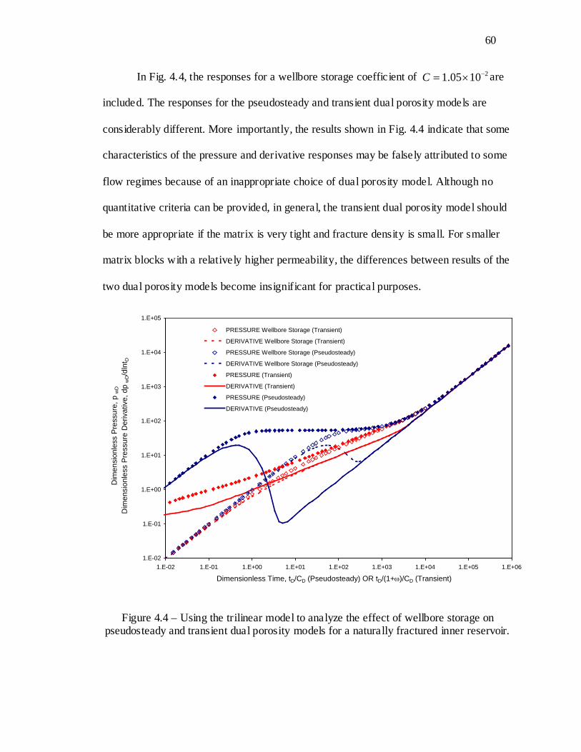
60

60

In Fig. 4.4, the responses for a wellbore storage coefficient of 21005.1 −×=C are

included. The responses for the pseudosteady and transient dual porosity models are

considerably different. More importantly, the results shown in Fig. 4.4 indicate that some

characteristics of the pressure and derivative responses may be falsely attributed to some

flow regimes because of an inappropriate choice of dual porosity model. Although no

quantitative criteria can be provided, in general, the transient dual porosity model should

be more appropriate if the matrix is very tight and fracture density is small. For smaller

matrix blocks with a relatively higher permeability, the differences between results of the

two dual porosity models become insignificant for practical purposes.

1.E-02

1.E-01

1.E+00

1.E+01

1.E+02

1.E+03

1.E+04

1.E+05

1.E-02 1.E-01 1.E+00 1.E+01 1.E+02 1.E+03 1.E+04 1.E+05 1.E+06

Dimensionless Time, tD/CD (Pseudosteady) OR tD/(1+ω)/CD (Transient)

Dim

ensi

onle

ss P

ress

ure,

p w

D

Dim

ensi

onle

ss P

ress

ure

Der

ivat

ive,

dp

wD/d

lnt D

PRESSURE Wellbore Storage (Transient)

DERIVATIVE Wellbore Storage (Transient)

PRESSURE Wellbore Storage (Pseudosteady)

DERIVATIVE Wellbore Storage (Pseudosteady)

PRESSURE (Transient)

DERIVATIVE (Transient)

PRESSURE (Pseudosteady)

DERIVATIVE (Pseudosteady)

Figure 4.4 – Using the trilinear model to analyze the effect of wellbore storage on pseudosteady and transient dual porosity models for a naturally fractured inner reservoir.

61

61

4.3 Asymptotic Approximations and Flow Regimes

Asymptotic approximations for the trilinear flow solution may be obtained by

considering the limiting forms of Eq. 3.95 for large and small values of the Laplace

transform parameter s – the limiting forms for large and small values of s are expected to

represent the early- and late-time behavior of the solution, respectively. Depending on the

relative values of s , ω , ω̂ , λ , and λ̂ , approximate forms of ( )sf , given in Eqs. 3.97,

3.98, and 3.99, are substituted into Eq. 3.95. Suitable approximations of ( )sf for

pseudosteady (Eq. 3.98) and transient (Eq. 3.99) dual porosity models are given,

respectively, by

( ) ( )

∞→−

→

=

s

ss

s

sf

as s,early timefor

of valuesteintermedia and timesteintermediafor 1

0 as times,latefor 1

ωω

λ (4.1)

and

( ) ( )

∞→

→+=

sss

ssf

as s,early timefor 1 of valuesteintermedia and timesteintermediafor 3ˆ

0 as times,latefor ˆ1ωλω

. (4.2)

Similarly, ( )αtanh may be replaced by the following approximations in deriving

asymptotic solutions:

( )

∞→−

→=

αααα

ααα

as1 of valuesteintermediafor 3

0 astanh 3 . (4.3)

It is possible to derive a large number of asymptotic approximations for the

trilinear flow solution by considering the above relationships. Below, a list of some of the

asymptotic approximations that can be derived for early, intermediate, and late times, are

62

62

presented. Some of these approximations may correspond to physical flow regimes

observed on field data depending on the relative values of ω and λ or ω̂ and λ̂ .

4.3.1 Early-Time Asymptotic Solution

It is possible to derive some early-time approximations for the trilinear flow

solution given by Eq. 3.95, but as discussed earlier, the trilinear flow model is not

applicable at very early times. In addition, the early-time behavior is dominated by the

wellbore storage effect and is therefore defined by the wellbore storage solution given in

Table 4.2.

Table 4.2 – Early-time asymptotic approximations to the trilinear model, pseudosteady and transient dual porosity models.

TRILINEAR MODEL EARLY-TIME ASYMPTOTIC APPROXIMATIONS,

Pseudosteady and Transient Dual Porosity Models

( )

( ) ( )[ ]

−

−=

gas,for 1422

and oil,for 2.141

pmpmqT

hk

ppqBhk

pi

II

iII

Dµ

( ) txc

ktFIt

ID 2µφ

= ( ) 22615.5

FID xch

CCφπ

=

Early-time Laplace transform parameter ∞→s

D

DwD C

tp =

4.3.2 Intermediate-Time Asymptotic Solutions

For the pseudosteady dual porosity model, Table 4.3 presents intermediate-time

approximations that may be derived. Similarly, Table 4.4 presents the intermediate-time

approximations which may be obtained for the transient dual porosity model.

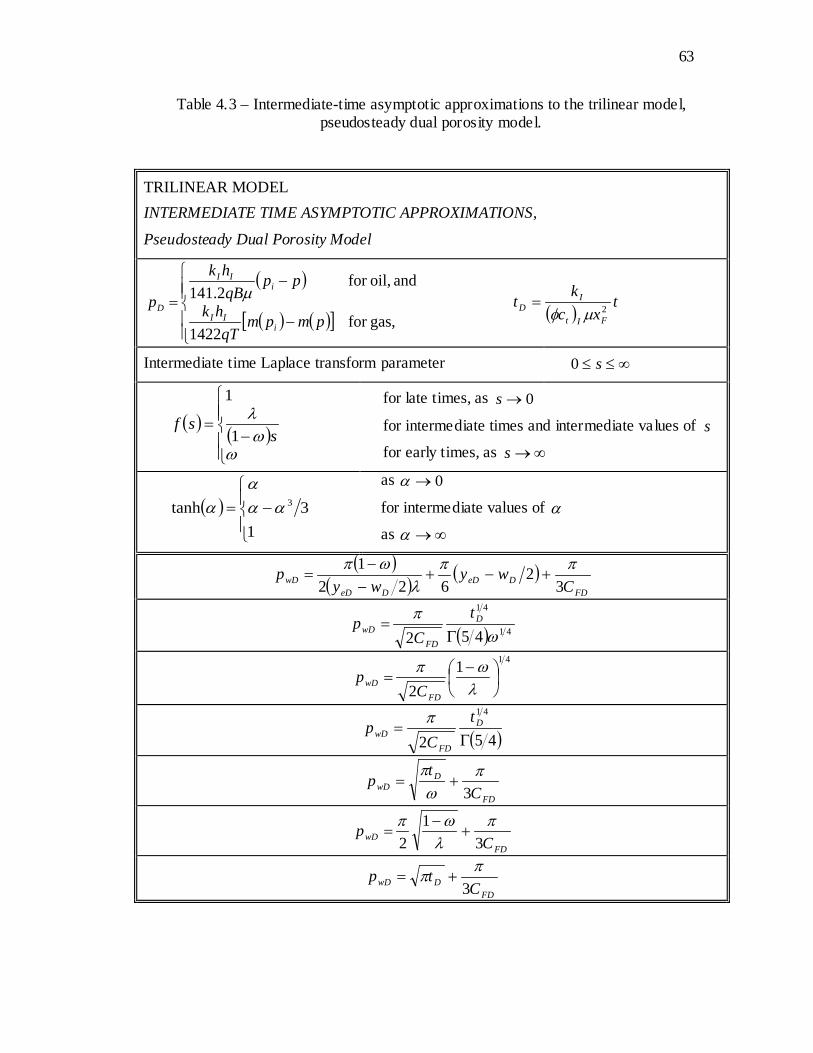
63

63

Table 4.3 – Intermediate-time asymptotic approximations to the trilinear model, pseudosteady dual porosity model.

TRILINEAR MODEL INTERMEDIATE TIME ASYMPTOTIC APPROXIMATIONS,

Pseudosteady Dual Porosity Model

( )

( ) ( )[ ]

−

−=

gas,for 1422

and oil,for 2.141

pmpmqT

hk

ppqBhk

pi

II

iII

Dµ

( ) txc

ktFIt

ID 2µφ

=

Intermediate time Laplace transform parameter ∞≤≤ s0

( ) ( )

−=

ωω

λs

sf1

1

for late times, as 0→s

for intermediate times and intermediate values of s

for early times, as ∞→s

( )

−=

13tanh 3αα

αα

as 0→α

for intermediate values of α

as ∞→α

( )( ) ( )

FDDeD

DeDwD C

wywy

p3

2622

1 ππλ

ωπ+−+

−−

=

( ) 41

41

452 ωπ

Γ= D

FDwD

tC

p

4112

−

=λ

ωπ

FDwD C

p

( )452

41

Γ= D

FDwD

tC

p π

FD

DwD C

tp

3π

ωπ

+=

FDwD C

p3

12

πλ

ωπ+

−=

FDDwD C

tp3

ππ +=

64

64

Table 4.4 – Intermediate time asymptotic approximations to the trilinear model, transient dual porosity model.

TRILINEAR MODEL INTERMEDIATE TIME ASYMPTOTIC APPROXIMATIONS,

Transient Dual Porosity Model

( )

( ) ( )[ ]

−

−=

gas,for 1422

and oil,for 2.141

pmpmqT

hk

ppqBhk

pi

II

iII

Dµ

( ) txc

ktFIt

ID 2µφ

=

Intermediate time Laplace transform parameter ∞≤≤ s0

( ) ( )

+=

13ˆ

ˆ1ssf ωλ

ω

for late times, as 0→s for intermediate times and intermediate values of s for early times, as ∞→s

( )

−=

13tanh 3αα

αα

as 0→α for intermediate values of α as ∞→α

( ) ( )FD

DeDDeD

DwD C

wywyt

p3

262

3 πππλω

+−+−

=

( )452

41

Γ= D

FDwD

tC

p π

( )892ˆˆ3 8181

99 Γ

= D

FDwD

tC

p πωλ

( )( ) 41

41

ˆ1452 ωπ

+Γ= D

FDwD

tC

p

FDDwD C

tp3

ππ +=

( ) FD

DwD C

tp345ˆˆ

32

4141 πωλ

π+

Γ

=

FD

DwD C

tp3ˆ1

πω

π+

+=

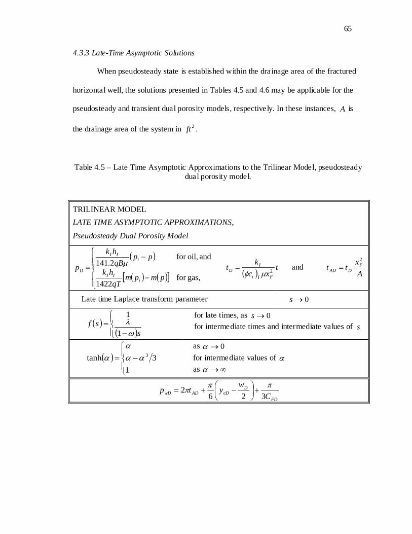
65

65

4.3.3 Late-Time Asymptotic Solutions

When pseudosteady state is established within the drainage area of the fractured

horizontal well, the solutions presented in Tables 4.5 and 4.6 may be applicable for the

pseudosteady and transient dual porosity models, respectively. In these instances, A is

the drainage area of the system in 2ft .

Table 4.5 – Late Time Asymptotic Approximations to the Trilinear Model, pseudosteady dual porosity model.

TRILINEAR MODEL LATE TIME ASYMPTOTIC APPROXIMATIONS,

Pseudosteady Dual Porosity Model

( )

( ) ( )[ ]

−

−=

gas,for 1422

and oil,for 2.141

pmpmqT

hk

ppqBhk

pi

II

iII

Dµ

( ) txc

ktFIt

ID 2µφ

= and A

xtt F

DAD

2

=

Late time Laplace transform parameter 0→s

( )( )

−=

ssf

ωλ

1

1

for late times, as 0→s for intermediate times and intermediate values of s

( )

−=

13tanh 3αα

αα

as 0→α for intermediate values of α as ∞→α

FD

DeDADwD C

wytp326

2 πππ +

−+=

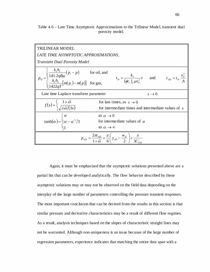
66

66

Table 4.6 – Late Time Asymptotic Approximations to the Trilinear Model, transient dual porosity model.

TRILINEAR MODEL LATE TIME ASYMPTOTIC APPROXIMATIONS,

Transient Dual Porosity Model

( )

( ) ( )[ ]

−

−=

gas,for 1422

and oil,for 2.141

pmpmqT

hk

ppqBhk

pi

II

iII

Dµ

( ) txc

ktFIt

ID 2µφ

= and A

xtt F

DAD

2

=

Late time Laplace transform parameter 0→s

( ) ( ) +

=s

sf3ˆˆ1

ωλω

for late times, as 0→s for intermediate times and intermediate values of s

( )

−=

13tanh 3αα

αα

as 0→α for intermediate values of α as ∞→α

FD

DeD

ADwD C

wytp326ˆ1

2 ππω

π+

−+

+=

Again, it must be emphasized that the asymptotic solutions presented above are a

partial list that can be developed analytically. The flow behavior described by these

asymptotic solutions may or may not be observed on the field data depending on the

interplay of the large number of parameters controlling the pressure transient responses.

The most important conclusion that can be derived from the results in this section is that

similar pressure and derivative characteristics may be a result of different flow regimes.

As a result, analysis techniques based on the slopes of characteristic straight lines may

not be warranted. Although non-uniqueness is an issue because of the large number of

regression parameters, experience indicates that matching the entire data span with a

67

67

model response, via regression analysis, usually converges to a better solution, or

diverges altogether. After an initial match is obtained, the results may be refined by

straight-line analysis using the asymptotic solutions given above.

4.4 Field Example

The following presents a field example to demonstrate the application of the

trilinear flow solution. The data for this example comes from a buildup test in a multiply

fractured horizontal well producing oil from a shale play. The tested section of the

horizontal well was the first ft302,1 from the tip of the well with seven transverse

fractures. At the time of testing, the rest of the horizontal well was cased and cemented,

but not perforated. Identical design and equal spacing was assumed for the fractures.

Therefore, the distance used between two fractures was ftft 2176302,1 = and the

distance from a fracture to the no-flow boundary between two fractures was

ftftye 5.1082217 == . For the trilinear model, th71 of the well flow rate was allocated

to each fracture ( 7qqF = ). A large value, ftxe 500,7= , was used for the half-distance

between two parallel horizontal wells, or the distance to a physical boundary, in the

model because there were no interfering wells in the reservoir. In the analysis, the

distance to the boundary in the x-direction was tested to verify that it had no influence on

the results.

Figure 4.5 shows the pressure and derivative responses from the data together

with the match obtained with the trilinear model. To clarify the example and hide the

identity of the data, some of the noise in the original data was removed without changing

the fundamental trend of the responses. Table 4.7 presents the pertinent information for

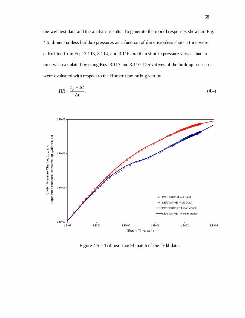
68

68

the well test data and the analysis results. To generate the model responses shown in Fig.

4.5, dimensionless buildup pressures as a function of dimensionless shut-in time were

calculated from Eqs. 3.113, 3.114, and 3.116 and then shut-in pressure versus shut-in

time was calculated by using Eqs. 3.117 and 3.110. Derivatives of the buildup pressures

were evaluated with respect to the Horner time ratio given by

t

ttHR p

∆

∆+= . (4.4)

1.E+00

1.E+01

1.E+02

1.E+03

1.E-02 1.E-01 1.E+00 1.E+01 1.E+02 1.E+03

Shut-in Time, ∆t, hr

Shu

t-in

Pre

ssur

e C

hang

e, ∆

p ws a

nd

Loga

rithm

ic P

ress

ure

Der

ivat

ive,

dp

ws/d

lnH

R, p

si

PRESSURE (Field Data)

DERIVATIVE (Field Data)

PRESSURE (Trilinear Mode)l

DERIVATIVE (Trilinear Model)

Figure 4.5 – Trilinear model match of the field data.

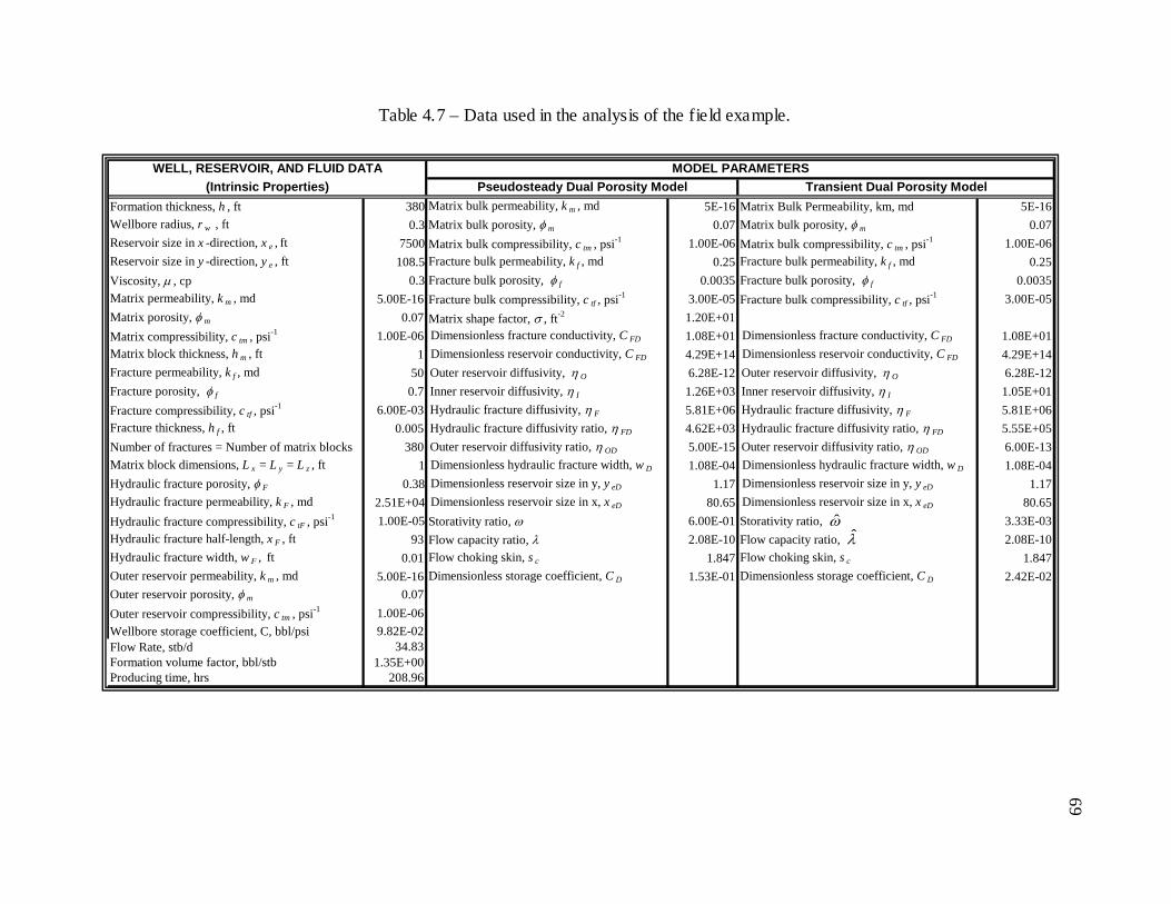
69 Table 4.7 – Data used in the analysis of the field example.

Formation thickness, h , ft 380 Matrix bulk permeability, k m , md 5E-16 Matrix Bulk Permeability, km, md 5E-16Wellbore radius, r w , ft 0.3 Matrix bulk porosity, φ m 0.07 Matrix bulk porosity, φ m 0.07Reservoir size in x -direction, x e , ft 7500 Matrix bulk compressibility, c tm , psi-1 1.00E-06 Matrix bulk compressibility, c tm , psi-1 1.00E-06Reservoir size in y -direction, y e , ft 108.5 Fracture bulk permeability, k f , md 0.25 Fracture bulk permeability, k f , md 0.25Viscosity, µ , cp 0.3 Fracture bulk porosity, φ f 0.0035 Fracture bulk porosity, φ f 0.0035Matrix permeability, k m , md 5.00E-16 Fracture bulk compressibility, c tf , psi-1 3.00E-05 Fracture bulk compressibility, c tf , psi-1 3.00E-05Matrix porosity, φ m 0.07 Matrix shape factor, σ , ft-2 1.20E+01Matrix compressibility, c tm , psi-1 1.00E-06 Dimensionless fracture conductivity, C FD 1.08E+01 Dimensionless fracture conductivity, C FD 1.08E+01Matrix block thickness, h m , ft 1 Dimensionless reservoir conductivity, C FD 4.29E+14 Dimensionless reservoir conductivity, C FD 4.29E+14Fracture permeability, k f , md 50 Outer reservoir diffusivity, η O 6.28E-12 Outer reservoir diffusivity, η O 6.28E-12Fracture porosity, φ f 0.7 Inner reservoir diffusivity, η I 1.26E+03 Inner reservoir diffusivity, η I 1.05E+01Fracture compressibility, c tf , psi-1 6.00E-03 Hydraulic fracture diffusivity, η F 5.81E+06 Hydraulic fracture diffusivity, η F 5.81E+06Fracture thickness, h f , ft 0.005 Hydraulic fracture diffusivity ratio, η FD 4.62E+03 Hydraulic fracture diffusivity ratio, η FD 5.55E+05Number of fractures = Number of matrix blocks 380 Outer reservoir diffusivity ratio, η OD 5.00E-15 Outer reservoir diffusivity ratio, η OD 6.00E-13Matrix block dimensions, L x = L y = L z , ft 1 Dimensionless hydraulic fracture width, w D 1.08E-04 Dimensionless hydraulic fracture width, w D 1.08E-04Hydraulic fracture porosity, φ F 0.38 Dimensionless reservoir size in y, y eD 1.17 Dimensionless reservoir size in y, y eD 1.17Hydraulic fracture permeability, k F , md 2.51E+04 Dimensionless reservoir size in x, x eD 80.65 Dimensionless reservoir size in x, x eD 80.65Hydraulic fracture compressibility, c tF , psi-1 1.00E-05 Storativity ratio, ω 6.00E-01 Storativity ratio, 3.33E-03Hydraulic fracture half-length, x F , ft 93 Flow capacity ratio, λ 2.08E-10 Flow capacity ratio, 2.08E-10Hydraulic fracture width, w F , ft 0.01 Flow choking skin, s c 1.847 Flow choking skin, s c 1.847Outer reservoir permeability, k m , md 5.00E-16 Dimensionless storage coefficient, C D 1.53E-01 Dimensionless storage coefficient, C D 2.42E-02Outer reservoir porosity, φ m 0.07Outer reservoir compressibility, c tm , psi-1 1.00E-06Wellbore storage coefficient, C, bbl/psi 9.82E-02Flow Rate, stb/d 34.83Formation volume factor, bbl/stb 1.35E+00Producing time, hrs 208.96

(Intrinsic Properties) Pseudosteady Dual Porosity Model Transient Dual Porosity ModelWELL, RESERVOIR, AND FLUID DATA MODEL PARAMETERS

λ̂ω̂

70

70

Several observations from the analysis of this field test are important to note: first,

except for the formation thickness and matrix porosity, most of the reservoir properties

were unknown or uncertain in the beginning of the analysis. Therefore, most of the

properties in the first column of Table 4.7 were considered as regression parameters

during the analysis. However, the analysis converged to the results shown in the second

column of Table 4.7 with reasonable confidence – small changes in the input data caused

discernable deviation of the model responses from the field data.

The second observation is that, for this particular example, the model responses

were not sensitive to the choice of dual porosity model. The fact that the pseudosteady

and transient dual porosity models yield the same responses is consistent with the

relatively large matrix permeability in this case, as opposed to the small matrix

permeability for the case given in Table 4.1 and the results shown in Figs. 4.3 and 4.4.

Third, there were initial difficulties in the interpretation of the flow rate history

and producing time. Fig. 4.6 shows the rate history before the shut-in of the well.

Inconsistencies in the pressure and rate behavior led to concerns about the use of

superposition to incorporate the effect of rate variations. Similarly, short interruptions of

the production period made it difficult to determine the start of the producing period or

the estimation of the effective producing time. Nevertheless, the data was analyzed

assuming a constant flow rate and effective producing time. Some flexibility in the flow

rate and effective producing time was allowed, however, in order to match the data with

the model responses. This point is important because the trilinear model indicated that the

characteristics of buildup responses were sensitive to producing time.

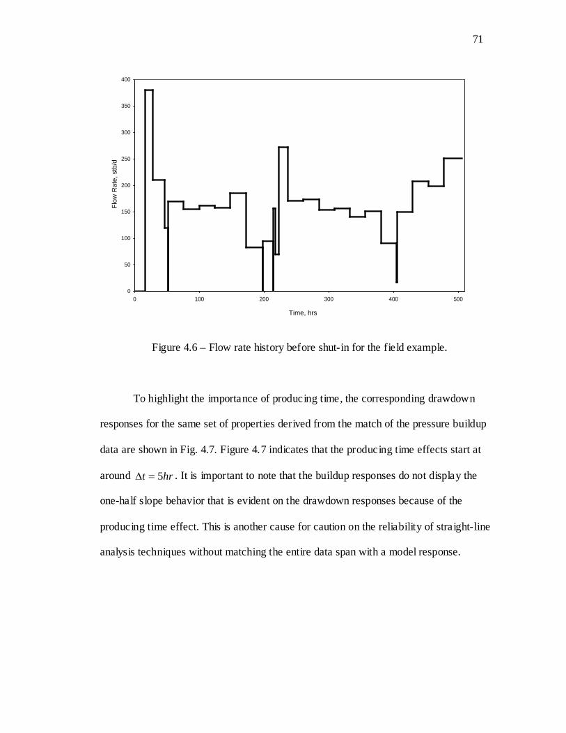
71

71

0

50

100

150

200

250

300

350

400

0 100 200 300 400 500

Time, hrs

Flow

Rat

e, s

tb/d

Figure 4.6 – Flow rate history before shut-in for the field example.

To highlight the importance of producing time, the corresponding drawdown

responses for the same set of properties derived from the match of the pressure buildup

data are shown in Fig. 4.7. Figure 4.7 indicates that the producing time effects start at

around hrt 5=∆ . It is important to note that the buildup responses do not display the

one-half slope behavior that is evident on the drawdown responses because of the

producing time effect. This is another cause for caution on the reliability of straight-line

analysis techniques without matching the entire data span with a model response.

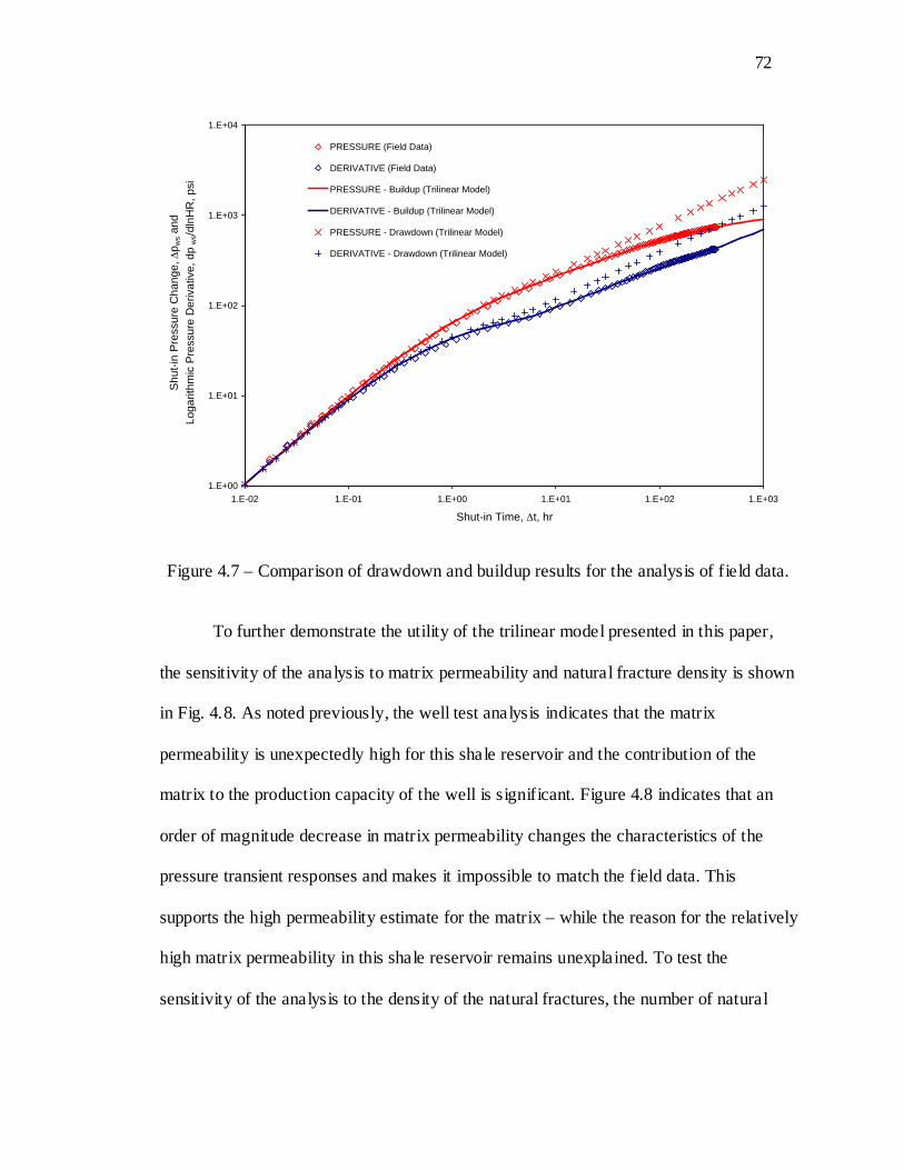
72

72

1.E+00

1.E+01

1.E+02

1.E+03

1.E+04

1.E-02 1.E-01 1.E+00 1.E+01 1.E+02 1.E+03

Shut-in Time, ∆t, hr

Shu

t-in

Pre

ssur

e C

hang

e, ∆

p ws a

nd

Loga

rithm

ic P

ress

ure

Der

ivat

ive,

dp

ws/d

lnH

R, p

si

PRESSURE (Field Data)

DERIVATIVE (Field Data)

PRESSURE - Buildup (Trilinear Model)

DERIVATIVE - Buildup (Trilinear Model)

PRESSURE - Drawdown (Trilinear Model)

DERIVATIVE - Drawdown (Trilinear Model)

Figure 4.7 – Comparison of drawdown and buildup results for the analysis of field data.

To further demonstrate the utility of the trilinear model presented in this paper,

the sensitivity of the analysis to matrix permeability and natural fracture density is shown

in Fig. 4.8. As noted previously, the well test analysis indicates that the matrix

permeability is unexpectedly high for this shale reservoir and the contribution of the

matrix to the production capacity of the well is significant. Figure 4.8 indicates that an

order of magnitude decrease in matrix permeability changes the characteristics of the

pressure transient responses and makes it impossible to match the field data. This

supports the high permeability estimate for the matrix – while the reason for the relatively

high matrix permeability in this shale reservoir remains unexplained. To test the

sensitivity of the analysis to the density of the natural fractures, the number of natural

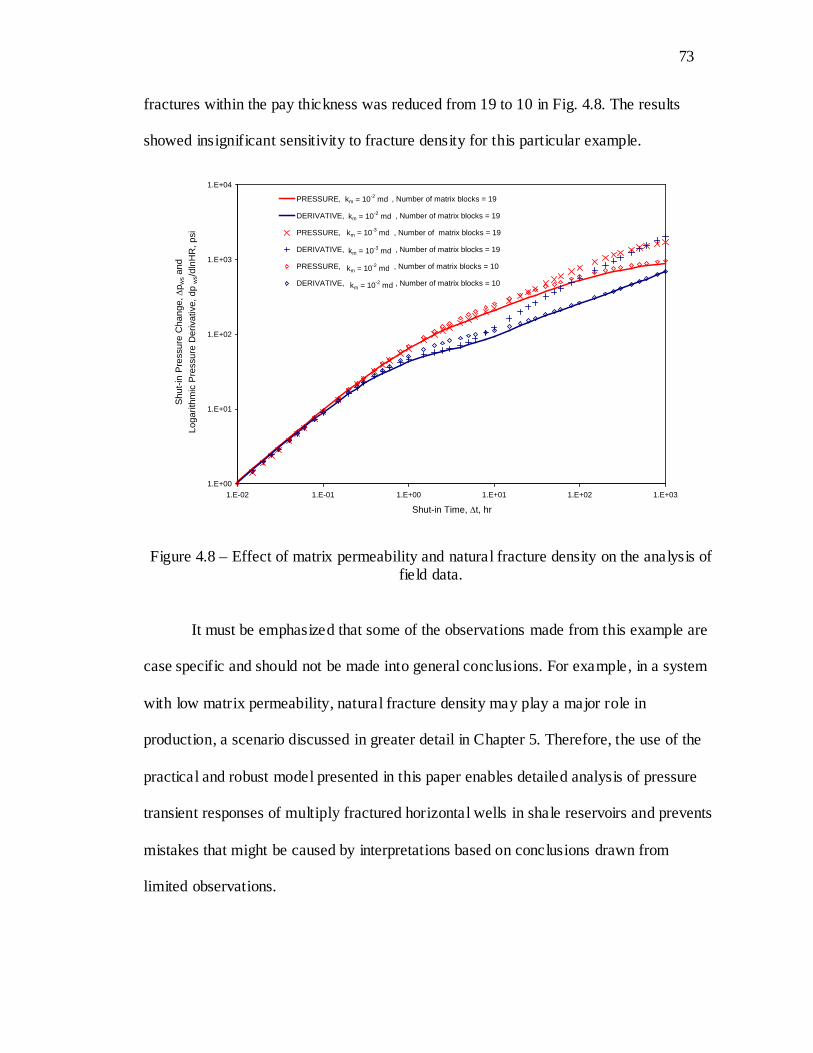
73

73

fractures within the pay thickness was reduced from 19 to 10 in Fig. 4.8. The results

showed insignificant sensitivity to fracture density for this particular example.

1.E+00

1.E+01

1.E+02

1.E+03

1.E+04

1.E-02 1.E-01 1.E+00 1.E+01 1.E+02 1.E+03

Shut-in Time, ∆t, hr

Shu

t-in

Pre

ssur

e C

hang

e, ∆

p ws a

nd

Loga

rithm

ic P

ress

ure

Der

ivat

ive,

dp

ws/d

lnH

R, p

siPRESSURE, , Number of matrix blocks = 19

DERIVATIVE, , Number of matrix blocks = 19

PRESSURE, , Number of matrix blocks = 19

DERIVATIVE, , Number of matrix blocks = 19

PRESSURE, , Number of matrix blocks = 10

DERIVATIVE, , Number of matrix blocks = 10

km = 10-2 md

km = 10-3 md

km = 10-2 md

km = 10-2 md

km = 10-2 md

km = 10-3 md

Figure 4.8 – Effect of matrix permeability and natural fracture density on the analysis of field data.

It must be emphasized that some of the observations made from this example are

case specific and should not be made into general conclusions. For example, in a system

with low matrix permeability, natural fracture density may play a major role in

production, a scenario discussed in greater detail in Chapter 5. Therefore, the use of the

practical and robust model presented in this paper enables detailed analysis of pressure

transient responses of multiply fractured horizontal wells in shale reservoirs and prevents

mistakes that might be caused by interpretations based on conclusions drawn from

limited observations.

74

74

CHAPTER 5

ANALYSIS OF RESULTS

Enabled by the relative simplicity of the trilinear model, this chapter continues the

discussion started in Chapter 4. Specifically, problems of design are addressed –

including the importance of both hydraulic and natural fracture conductivity and density

to productivity of the well. The method used for determining the productivity index is

presented in the last section of this chapter.

Recalling the discussion in Chapter 4 on use of the pseudosteady state versus

transient dual porosity models (Figs. 4.3 and 4.4), in general, the transient dual porosity

model should be more appropriate if the matrix is very tight and fracture density is small,

a situation typically found in shale formations. Unless otherwise noted, Table 5.1

presents the reservoir, matrix, hydraulic fracture, and natural fracture properties used for

all analyses in this chapter – including a matrix permeability of md6101 −× . Due to the

low matrix permeability, the analysis of results in Chapter 5 is facilitated by the use of

the transient dual porosity model (Kazemi, 1969, de Swaan-O, 1976, and Serra et al.,

1983) in terms of intrinsic properties of the fracture and matrix media. Specifically,

ftfI hkhk = where fk is the intrinsic permeability of the natural fractures and fth is the

total thickness of the natural fractures intersecting the height of the hydraulic fracture,

Fh . In this work, Fh is equal to the thickness of the pay zone, h . If fn is the count of

natural fractures intersecting the height of the hydraulic fracture, and fh is the aperture

75

75

of the natural fractures, then ffft hnh = . Furthermore, the density of natural fractures,

hn ff =ρ , in units of natural fracture count per foot of pay zone ( ftf ) is introduced.

An estimate of fρ may be obtained from cores, logs, or rate of penetration data, for

example.

Table 5.1 – Data used in Chapter 5 analyses, unless otherwise noted.

Formation thickness, h , ft 250 Matrix permeability, k m , md 1.0E-06Temperature, ºF 150 Matrix porosity, φ m 0.05Specific Gravity, γ 0.55 Matrix compressibility, c tm , psi-1 1.0E-05Reservoir pressure, initial, psi 4,000Viscosity, µ , cp 0.0184Reservoir size in x -direction, x e , ft 500Flow rate, q F,sc , Mscf/D 100

Hydraulic fracture permeability, k F , md 1.0E+05 Fracture permeability, k f , md 2,000Hydraulic fracture width, w F , ft 1.0E-02 Fracture thickness, h f , ft 1.0E-03Hydraulic fracture porosity, φ F 0.38 Fracture porosity, φ f 0.45Hydraulic fracture compressibility, c tF , psi-1 1.0E-05 Fracture compressibility, c tf , psi-1 1.0E-05Hydraulic fracture half-length, x F , ft 250 Fracture denisty, ρ f , f/ft 0.80Distance between hydraulic fractures, d F , ft 500

NATURAL FRACTURESHYDRAULIC FRACTURES

MATRIXRESERVOIR

5.1 Effect of the Outer Reservoir

The following discussion presents results in support of field observations that the

drainage of fractured horizontal wells in shale formations is confined to the inner

reservoir between hydraulic fractures – also referred to as the stimulated volume. A dry

gas reservoir is considered and results are presented in terms of pseudopressure to

facilitate the identification of conventional flow regimes.

In Figs. 5.1 and 5.2, pseudopressure change, wfiwD mmm −=∆ , is presented as a

function of time for three different distances to the outer reservoir boundary – the

76

76

distance to the outer boundary, ex , corresponds to the half of the horizontal well spacing

in the field. In all figures, the case corresponding to ftxx Fe 250== represents the

condition where the drainage volume is limited to the inner reservoir, and therefore, the

deviation of pseudopressures from the Fe xx = case indicates the support of the outer

reservoir.

Prior to discussing the results in Figs. 5.1 and 5.2, the value of the matrix

permeability used in these two simulations, mdkm 1000= , must be addressed. When

matrix permeabilities in the millidarcy range were used, no influence of the outer

reservoir was observed. This result can be explained by the fact that the outer reservoir is

assumed to be made out of the same matrix, though without natural fractures. A tighter

matrix causes a faster pressure drop in the inner zone, but the support of the outer zone is

also less efficient, and takes a longer period of time to be felt. Therefore, the cases

presented in Figs. 5.1 and 5.2 may not correspond to tight, shale reservoirs, but they do

allow for observations on the general characteristics of support from the outer reservoir.

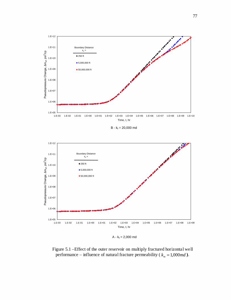
77

77

B - kf = 20,000 md

1.E+05

1.E+06

1.E+07

1.E+08

1.E+09

1.E+10

1.E+11

1.E+12

1.E-03 1.E-02 1.E-01 1.E+00 1.E+01 1.E+02 1.E+03 1.E+04 1.E+05 1.E+06 1.E+07 1.E+08 1.E+09 1.E+10

Time, t, hr

Pse

udop

ress

ure

Cha

nge,

Δm

wf,

psi2 /c

p

250 ft

5,000,000 ft

50,000,000 ft

Boundary Distancexe =

A - kf = 2,000 md

1.E+05

1.E+06

1.E+07

1.E+08

1.E+09

1.E+10

1.E+11

1.E+12

1.E-03 1.E-02 1.E-01 1.E+00 1.E+01 1.E+02 1.E+03 1.E+04 1.E+05 1.E+06 1.E+07 1.E+08 1.E+09

Time, t, hr

Pse

udop

ress

ure

Cha

nge,

Δm

wf,

psi2 /c

p

250 ft

5,000,000 ft

50,000,000 ft

Boundary Distancexe =

Figure 5.1 –Effect of the outer reservoir on multiply fractured horizontal well performance – influence of natural fracture permeability ( mdkm 000,1= ).

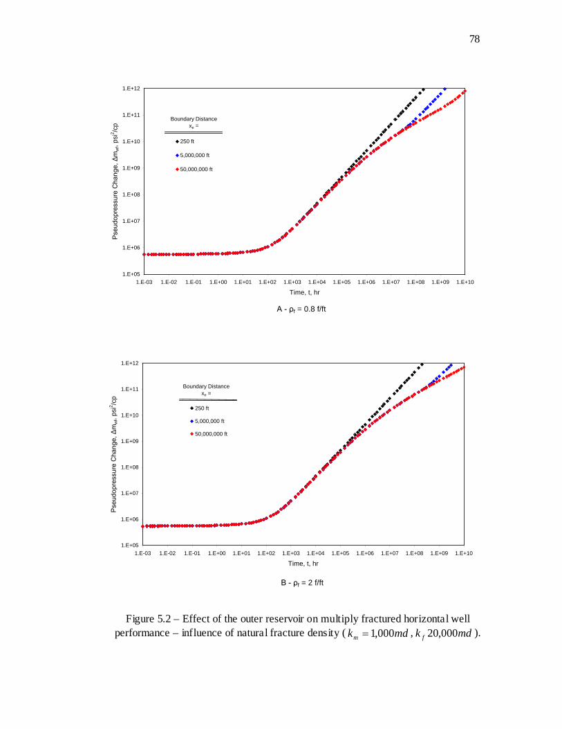
78

78

A - ρf = 0.8 f/ft

1.E+05

1.E+06

1.E+07

1.E+08

1.E+09

1.E+10

1.E+11

1.E+12

1.E-03 1.E-02 1.E-01 1.E+00 1.E+01 1.E+02 1.E+03 1.E+04 1.E+05 1.E+06 1.E+07 1.E+08 1.E+09 1.E+10

Time, t, hr

Pse

udop

ress

ure

Cha

nge,

Δm

wf,

psi2 /c

p

250 ft

5,000,000 ft

50,000,000 ft

Boundary Distancexe =

B - ρf = 2 f/ft

1.E+05

1.E+06

1.E+07

1.E+08

1.E+09

1.E+10

1.E+11

1.E+12

1.E-03 1.E-02 1.E-01 1.E+00 1.E+01 1.E+02 1.E+03 1.E+04 1.E+05 1.E+06 1.E+07 1.E+08 1.E+09 1.E+10

Time, t, hr

Pse

udop

ress

ure

Cha

nge,

Δm

wf,

psi2 /c

p

250 ft

5,000,000 ft

50,000,000 ft

Boundary Distancexe =

Figure 5.2 – Effect of the outer reservoir on multiply fractured horizontal well performance – influence of natural fracture density ( mdkm 000,1= , mdk f 000,20 ).

79

79

In Fig. 5.1.B, the natural fracture permeability is increased to mdk f 000,20= ,

which may not be realistic for most natural fractures. However, this case may be used to

simulate a hydraulic fracture network, resulting from dense, complex, hydraulic fracture

growth, with a natural fracture density of ftff 8.0=ρ . Comparing the results in Figs.

5.1.A and 5.1.B with each other, it is apparent that higher natural fracture permeability

causes the support of the outer reservoir to become evident earlier; however, the effect of

the outer reservoir is still outside of the practical life span of the well. These observations

support the common practice of small well spacing to efficiently drain tight, shale

reservoirs with fractured horizontal wells.

Figure 5.2 demonstrates the effect of natural fracture density on the contribution

of the outer reservoir. Figure 5.2.A is the same as Figure 5.1.B, both having a natural

fracture density of ftff 8.0=ρ . In Fig. 5.2.B, the fracture density is increased to

ftff 2=ρ . By comparing the results in Figs. 5.2.A and 5.2.B with each other, it

becomes apparent that a higher fracture density does not cause a noticeable change in the

time required to feel the effect of the outer reservoir. Moreover, though a higher fracture

density yields a more significant contribution of the outer reservoir at late times, the

effect only becomes evident at impractically late times. The discussion in this section

therefore indicates that, for practical shale matrix permeabilities, fractured horizontal

wells do not drain the region beyond the tips of the hydraulic fractures.

5.2 Effect of Matrix Permeability

When the matrix permeability decreases from milli- to micro- and nano- Darcy

range, the reservoir description is changed from conventional to unconventional. Due to

80

80

their much smaller matrix permeabilities, unconventional shale reservoirs require a dense

fracture network to achieve a sufficient effective permeability. The effect of matrix

permeability when the inner reservoir is naturally fractured, as in unconventional tight

shale formations, is presented first. Then, a comparison with a case where there are no

natural fractures, as in conventional tight sand applications, is presented.

Figure 5.3 shows the pseudopressure change versus time (Fig. 5.3.A) and log-

derivative versus time (Fig. 5.3.B) for matrix permeabilities in the range of

mdkmd m18 1010 −− ≤≤ . In Fig. 5.3.A, pseudopressure responses are also shown for the

idealized case where there is no flow choking around the intersection of the horizontal

well and hydraulic fracture (see Section 3.6 for choking skin calculation). Figure 5.3.A

indicates that the choking skin masks the characteristic early-time responses of multiply

fractured horizontal wells in naturally fractured reservoirs. The derivative responses in

Fig. 5.3.B, however, are not influenced by the choking skin and display all early-time

flow characteristics. This observation emphasizes the importance of derivative analysis

for multiply fractured horizontal wells in shale – especially for the identification of flow

characteristics from production data where derivative analysis may not be possible or

may be overlooked.

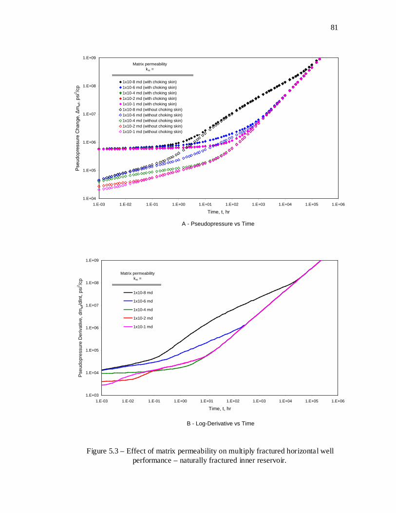
81

81

A - Pseudopressure vs Time

1.E+04

1.E+05

1.E+06

1.E+07

1.E+08

1.E+09

1.E-03 1.E-02 1.E-01 1.E+00 1.E+01 1.E+02 1.E+03 1.E+04 1.E+05 1.E+06

Time, t, hr

Pse

udop

ress

ure

Cha

nge,

Δm

wf,

psi2 /c

p1x10-8 md (with choking skin)1x10-6 md (with choking skin)1x10-4 md (with choking skin)1x10-2 md (with choking skin)1x10-1 md (with choking skin)1x10-8 md (without choking skin)1x10-6 md (without choking skin)1x10-4 md (without choking skin)1x10-2 md (without choking skin)1x10-1 md (without choking skin)

Matrix permeabilitykm =

B - Log-Derivative vs Time

1.E+03

1.E+04

1.E+05

1.E+06

1.E+07

1.E+08

1.E+09

1.E-03 1.E-02 1.E-01 1.E+00 1.E+01 1.E+02 1.E+03 1.E+04 1.E+05 1.E+06

Time, t, hr

Pse

udop

ress

ure

Der

ivat

ive,

dm

wf/d

lnt,

psi2 /c

p

1x10-8 md

1x10-6 md

1x10-4 md

1x10-2 md

1x10-1 md

Matrix permeabilitykm =

Figure 5.3 – Effect of matrix permeability on multiply fractured horizontal well performance – naturally fractured inner reservoir.

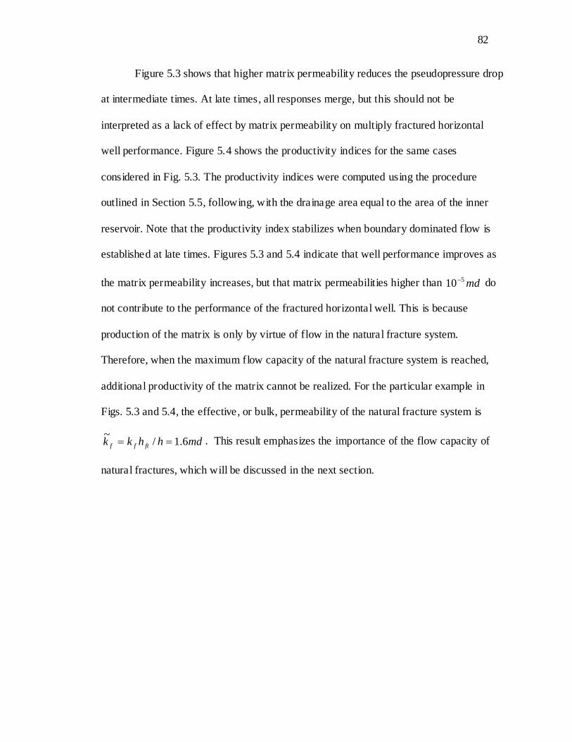
82

82

Figure 5.3 shows that higher matrix permeability reduces the pseudopressure drop

at intermediate times. At late times, all responses merge, but this should not be

interpreted as a lack of effect by matrix permeability on multiply fractured horizontal

well performance. Figure 5.4 shows the productivity indices for the same cases

considered in Fig. 5.3. The productivity indices were computed using the procedure

outlined in Section 5.5, following, with the drainage area equal to the area of the inner

reservoir. Note that the productivity index stabilizes when boundary dominated flow is

established at late times. Figures 5.3 and 5.4 indicate that well performance improves as

the matrix permeability increases, but that matrix permeabilities higher than md510− do

not contribute to the performance of the fractured horizontal well. This is because

production of the matrix is only by virtue of flow in the natural fracture system.

Therefore, when the maximum flow capacity of the natural fracture system is reached,

additional productivity of the matrix cannot be realized. For the particular example in

Figs. 5.3 and 5.4, the effective, or bulk, permeability of the natural fracture system is

mdhhkk ftff 6.1/~== . This result emphasizes the importance of the flow capacity of

natural fractures, which will be discussed in the next section.

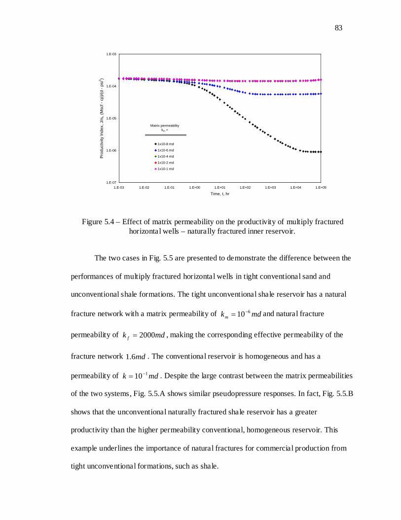
83

83

1.E-07

1.E-06

1.E-05

1.E-04

1.E-03

1.E-03 1.E-02 1.E-01 1.E+00 1.E+01 1.E+02 1.E+03 1.E+04 1.E+05

Time, t, hr

Pro

duct

ivity

Inde

x, J

/nf,

(Msc

f - c

p)/(d

- ps

i2 )

1x10-8 md

1x10-6 md

1x10-4 md

1x10-2 md

1x10-1 md

Matrix permeabilitykm =

Figure 5.4 – Effect of matrix permeability on the productivity of multiply fractured horizontal wells – naturally fractured inner reservoir.

The two cases in Fig. 5.5 are presented to demonstrate the difference between the

performances of multiply fractured horizontal wells in tight conventional sand and

unconventional shale formations. The tight unconventional shale reservoir has a natural

fracture network with a matrix permeability of mdkm610−= and natural fracture

permeability of mdk f 2000= , making the corresponding effective permeability of the

fracture network md6.1 . The conventional reservoir is homogeneous and has a

permeability of mdk 110−= . Despite the large contrast between the matrix permeabilities

of the two systems, Fig. 5.5.A shows similar pseudopressure responses. In fact, Fig. 5.5.B

shows that the unconventional naturally fractured shale reservoir has a greater

productivity than the higher permeability conventional, homogeneous reservoir. This

example underlines the importance of natural fractures for commercial production from

tight unconventional formations, such as shale.

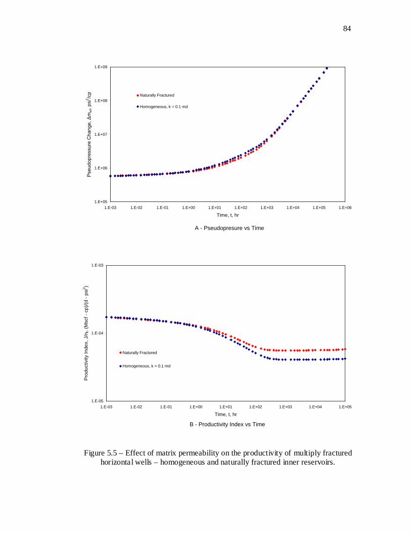
84

84

A - Pseudopresure vs Time

1.E+05

1.E+06

1.E+07

1.E+08

1.E+09

1.E-03 1.E-02 1.E-01 1.E+00 1.E+01 1.E+02 1.E+03 1.E+04 1.E+05 1.E+06

Time, t, hr

Pse

udop

ress

ure

Cha

nge,

Δm

wf,

psi2 /c

p Naturally Fractured

Homogeneous, k = 0.1 md

B - Productivity Index vs Time

1.E-05

1.E-04

1.E-03

1.E-03 1.E-02 1.E-01 1.E+00 1.E+01 1.E+02 1.E+03 1.E+04 1.E+05

Time, t, hr

Pro

duct

ivity

Inde

x, J

/nf,

(Msc

f - c

p)/(d

- ps

i2 )

Naturally Fractured

Homogeneous, k = 0.1 md

Figure 5.5 – Effect of matrix permeability on the productivity of multiply fractured horizontal wells – homogeneous and naturally fractured inner reservoirs.

85

85

5.3 Effect of Natural Fracture Permeability and Density

In the previous section, the importance of the flow capacity of natural fractures

for production from tight shale formations was emphasized. Figures 5.6 and 5.7 both

indicate that natural fractures with high permeability may not significantly improve well

productivity, whereas a high density of natural fractures may have a significant effect on

productivity. This is due to the relative flow capacities of the matrix and fracture systems,

as discussed in the previous section. Increasing permeability increases the flow capacity

of natural fractures, but it does not change the flow capacity of the matrix, because flow

capacity is proportional to surface area. If there is not enough fluid transfer from the

matrix to the fracture, an increased permeability in the natural fractures will not create

additional productivity.

However, a greater density of natural fractures increases the flow capacities of

both the natural fractures and the matrix because of the increase in surface area that is

available for fluid transfer. This therefore leads to a more significant increase in

productivity. From a practical viewpoint, this is a desirable feature because increasing the

permeability of natural fractures may not be a viable option, while increasing the density

of natural fractures may be accomplished by designing complex hydraulic fractures in

brittle formations. It may also be deduced that creating a complex hydraulic fracture

network of high permeability, but relatively low density, is not a good option if the

hydraulic fracturing does not also increase the density of the natural fractures. This

indicates that the experience in brittle shale formations, such as the Barnett, cannot be

directly extrapolated to soft shale formations, such as the Marcellus.

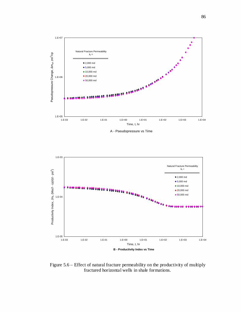
86

86

A - Pseudopressure vs Time

1.E+05

1.E+06

1.E+07

1.E-03 1.E-02 1.E-01 1.E+00 1.E+01 1.E+02 1.E+03 1.E+04

Time, t, hr

Pse

udop

ress

ure

Cha

nge,

Δm

wf,

psi2 /c

p

2,000 md

5,000 md

10,000 md

20,000 md

50,000 md

Natural Fracture Permeabilitykf =

B - Productivity Index vs Time

1.E-05

1.E-04

1.E-03

1.E-03 1.E-02 1.E-01 1.E+00 1.E+01 1.E+02 1.E+03 1.E+04

Time, t, hr

Pro

duct

ivity

Inde

x, J

/nf,

(Msc

f - c

p)/(d

- ps

i2 )

2,000 md

5,000 md

10,000 md

20,000 md

50,000 md

Natural Fracture Permeabilitykf =

Figure 5.6 – Effect of natural fracture permeability on the productivity of multiply fractured horizontal wells in shale formations.

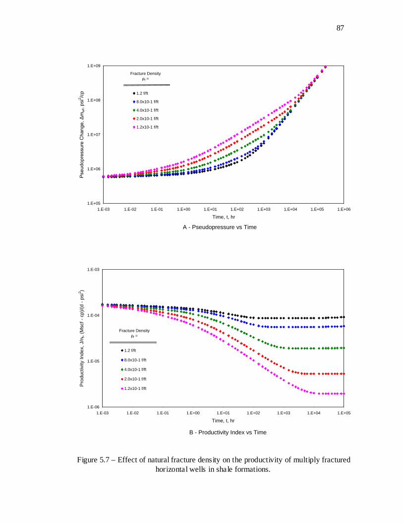
87

87

A - Pseudopressure vs Time

1.E+05

1.E+06

1.E+07

1.E+08

1.E+09

1.E-03 1.E-02 1.E-01 1.E+00 1.E+01 1.E+02 1.E+03 1.E+04 1.E+05 1.E+06

Time, t, hr

Pse

udop

ress

ure

Cha

nge,

Δm

wf,

psi2 /c

p 1.2 f/ft

8.0x10-1 f/ft

4.0x10-1 f/ft

2.0x10-1 f/ft

1.2x10-1 f/ft

Fracture Density ρf =

B - Productivity Index vs Time

1.E-06

1.E-05

1.E-04

1.E-03

1.E-03 1.E-02 1.E-01 1.E+00 1.E+01 1.E+02 1.E+03 1.E+04 1.E+05

Time, t, hr

Pro

duct

ivity

Inde

x, J

/nf,

(Msc

f - c

p)/(d

- ps

i2 )

1.2 f/ft

8.0x10-1 f/ft

4.0x10-1 f/ft

2.0x10-1 f/ft

1.2x10-1 f/ft

Fracture Density ρf =

Figure 5.7 – Effect of natural fracture density on the productivity of multiply fractured horizontal wells in shale formations.

88

88

5.4 Effect of Hydraulic Fracture Permeability and Spacing

Determining the optimum number of hydraulic fractures to be created along the

length of the well is an important practical concern. A relevant, but more conventional,

concern is determining the optimum conductivity of hydraulic fractures. Figure 5.8 is a

demonstration of the conventional concept that increasing hydraulic fracture

conductivity, FF wk , leads to an increase in productivity. The incremental benefit,

however, decreases as the conductivity increases. From a fundamental viewpoint, higher

productivity is achieved by making the dimensionless conductivity, ( )FFFFD kxwkC = ,

larger. This concept is relatively straightforward for the design of hydraulic fractures in

conventional tight formations, such as tight gas sands, where higher conductivities can be

achieved for low reservoir permeability, k . A large dimensionless conductivity indicates

that the hydraulic fracture can transmit all the fluid provided by the reservoir.

For tight shale formations, dimensionless hydraulic fracture conductivity is

defined based on the effective fracture permeability ( fkk ~= ) and may appear to be

relatively large. This can be misleading. As discussed in the previous section, due to low

matrix permeability or low surface area because of a low natural fracture density, the

flow capacity of the matrix may not be sufficient to supply the fracture network to its full

capacity. Higher dimensionless fracture conductivities, achieved by creating a greater

density of natural fractures, are therefore desirable. It must be noted, however, that

greater natural fracture densities increase the effective natural fracture permeability and

decrease the dimensionless hydraulic fracture conductivity. This leads to a more complex

design problem for hydraulic fractures in tight, naturally fractured shale formations.

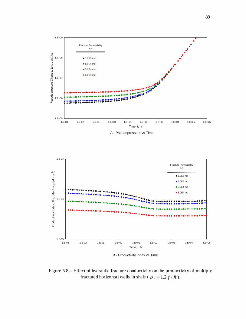
89

89

A - Pseudopressure vs Time

1.E+05

1.E+06

1.E+07

1.E+08

1.E+09

1.E-03 1.E-02 1.E-01 1.E+00 1.E+01 1.E+02 1.E+03 1.E+04 1.E+05 1.E+06

Time, t, hr

Pse

udop

ress

ure

Cha

nge,

Δm

wf,

psi2 /c

p

1.0E5 md

8.0E4 md

5.0E4 md

3.0E4 md

Fracture Permeability kf =

B - Productivity Index vs Time

1.E-05

1.E-04

1.E-03

1.E-03 1.E-02 1.E-01 1.E+00 1.E+01 1.E+02 1.E+03 1.E+04 1.E+05

Time, t, hr

Pro

duct

ivity

Inde

x, J

/nf,

(Msc

f - c

p)/(d

- ps

i2 )

1.0E5 md

8.0E4 md

5.0E4 md

3.0E4 md

Fracture Permeability kf =

Figure 5.8 – Effect of hydraulic fracture conductivity on the productivity of multiply fractured horizontal wells in shale ( ftff 2.1=ρ ).

90

90

As shown in Fig. 5.9.A, reducing the hydraulic fracture spacing significantly

influences the magnitudes of the intermediate- and late-time pseudopressures. On the

other hand, Fig. 5.9.B shows that hydraulic fracture spacing does not significantly change

flow characteristics, it does, however, effect the duration of flow regimes. It must be

noted that the flow rate of each fracture has been kept constant while changing the

hydraulic fracture spacing in Fig. 5.9. If the total flow rate were kept constant, then the

individual fracture rates would have to be reduced when the well spacing decreased. This

would yield a separation of the pseudopressure curves at early times – with the smallest

pseudopressure change corresponding with the smaller fracture spacing.

The productivity of each fracture is expected to increase when the fracture

spacing is decreased. As shown in Fig. 5.10.A, however, the incremental gain in

productivity with each additional fracture decreases. To find the total productivity of the

system, the productivity indices in Fig. 5.10 must be multiplied by the corresponding

number of hydraulic fractures. For example, for a ft000,4 horizontal well, a hydraulic

fracture spacing of ft000,1 corresponds to two hydraulic fractures, and a spacing of

ft250 corresponds to eight hydraulic fractures. The total productivity of the well with

ft000,1 fracture spacing is then obtained by multiplying the corresponding individual

fracture productivities given in Fig. 5.10 by two. Similarly, the well productivity for

ft250 fracture spacing would be obtained by multiplying the corresponding productivity

index by eight. This would yield a larger productivity for the well with eight fractures

( ft250 spacing) than with two fractures ( ft000,1 spacing).

91

91

A - Pseudopressue vs Time

1.E+05

1.E+06

1.E+07

1.E+08

1.E+09

1.E-03 1.E-02 1.E-01 1.E+00 1.E+01 1.E+02 1.E+03 1.E+04 1.E+05 1.E+06

Time, t, hr

Pse

udop

ress

ure

Cha

nge,

Δm

wf,

psi2 /c

p

1,000 ft

750 ft

500 ft

250 ft

Hydraulic Fracture Spacingdf =

B - Log-Derivative vs Time

1.E+04

1.E+05

1.E+06

1.E+07

1.E+08

1.E+09

1.E-03 1.E-02 1.E-01 1.E+00 1.E+01 1.E+02 1.E+03 1.E+04 1.E+05 1.E+06

Time, t, hr

Pse

udop

ress

ure

Der

ivat

ive,

dm

wf /

dln

t, ps

i2 /cp

1,000 ft

750 ft

500 ft

250 ft

Hydraulic Fracture Spacingdf =

Figure 5.9 – Effect of hydraulic fracture spacing on the pseudopressure responses of multiply fractured horizontal wells in shale ( ftff 4.0=ρ ).

92

92

A - Effect of Hydraulic Fracture Spacing for Fixed Natural Fracture Density

1.E-05

1.E-04

1.E-03

1.E-03 1.E-02 1.E-01 1.E+00 1.E+01 1.E+02 1.E+03 1.E+04 1.E+05

Time, t, hr

Pro

duct

ivity

Inde

x, J

/nf,

(Msc

f - c

p)/(d

- ps

i2 )1,000 ft

750 ft

500 ft

250 ft

Hydraulic Fracture Spacingdf =

Figure 5.10 – Effect of hydraulic fracture spacing and natural fracture density on the productivity of fractured horizontal wells in shale (in A, ftff 4.0=ρ ).

B - Combined Effect of Hydraulic Fracture Spacing and Natural Fracture Density

1.E-05

1.E-04

1.E-03

1.E-03 1.E-02 1.E-01 1.E+00 1.E+01 1.E+02 1.E+03 1.E+04 1.E+05

Time, t, hr

Pro

duct

ivity

Inde

x, J

/nf,

(Msc

f - c

p)/(d

- ps

i2 )

1,000 ft, 1.2 f/ft

250 ft, 1.2 f/ft

1,000 ft, 0.4 f/ft

250 ft, 0.4 f/ft

Hydraulic Fracture Spacing and

Natural Fracture Density df = , ρf =

93

93

To complete the discussion, Fig. 5.10.B presents individual fracture productivities

for two values of natural fracture density and two values of hydraulic fracture spacing. As

expected, Fig. 5.10.B indicates that increasing natural fracture density while decreasing

hydraulic fracture spacing provides the greatest productivity increase. This conclusion

supports the field practice of creating complex fractures to increase natural fracture

density and simultaneously decreasing hydraulic fracture spacing.

5.5 Computation of the Productivity Index

The productivity index of a multiply fractured horizontal well is defined by

wf

FF

wf ppqn

ppqJ

−=

−= ~~ (5.1)

for liquid flow, where p~ denotes the average pressure in the reservoir, Fn is the number

of hydraulic fractures, and Fq is the flow rate of each individual fracture. Equation 5.1

may be rewritten to yield

( )DwD

I

F

FF

pphk

Bqq

nJ~2.141

−=

µ, (5.2)

where wDp is computed from Eq. 3.111 and

( )

+

=modelporosity dualent for transi

ˆ12

modelporosity dualdy pseudosteafor 2~

D

D

D

D

D

At

At

p

ωπ

π, (5.3)

with

2F

D xAA = . (5.4)

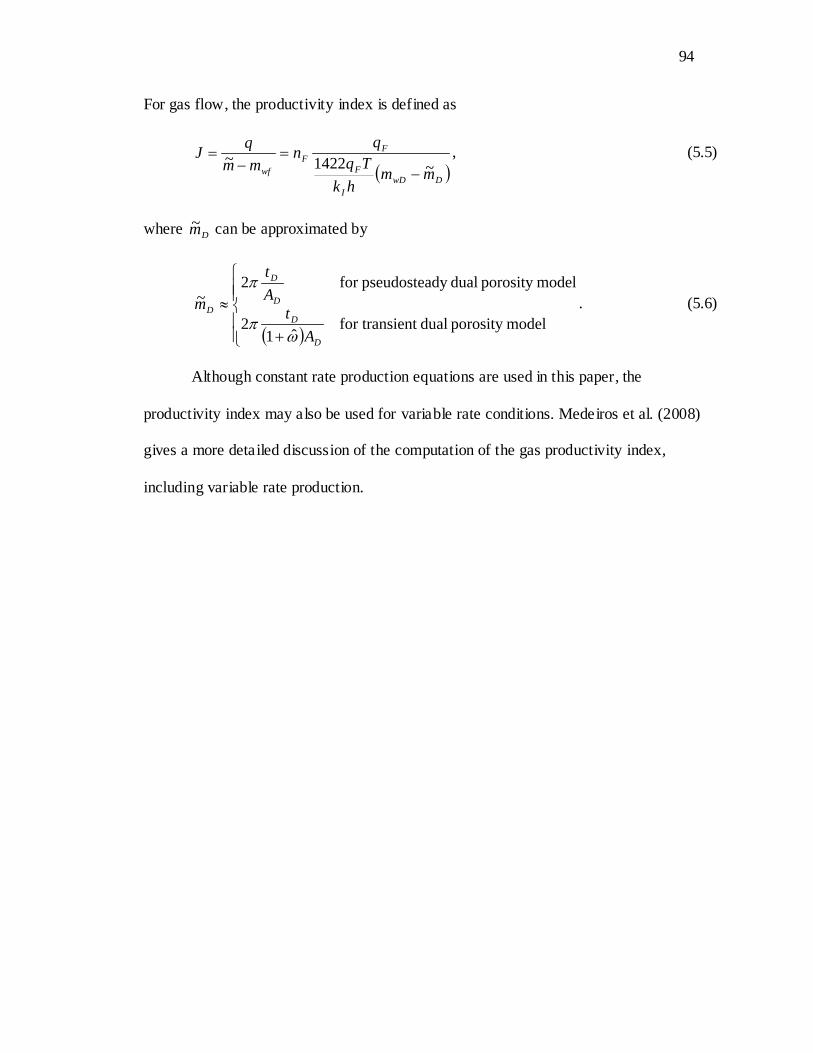
94

94

For gas flow, the productivity index is defined as

( )DwD

I

F

FF

wf mmhk

Tqqn

mmqJ

~1422~−

=−

= , (5.5)

where Dm~ can be approximated by

( )

+

≈modelporosity dualent for transi

ˆ12

modelporosity dualdy pseudosteafor 2~

D

D

D

D

D

At

At

m

ωπ

π. (5.6)

Although constant rate production equations are used in this paper, the

productivity index may also be used for variable rate conditions. Medeiros et al. (2008)

gives a more detailed discussion of the computation of the gas productivity index,

including variable rate production.

95

95

CHAPTER 6

CONCLUSIONS AND RECOMMENDATIONS

In this thesis, an analytical trilinear flow model has been developed and presented

that acknowledges the linear flow convergence prevailing in multiply fractured horizontal

wells in tight shale formations. The practicality of the new model has been demonstrated

by the examples presented herein.

This chapter presents major characteristics, advantages, and disadvantages of the

trilinear model as discussed in previous chapters. It also presents areas that may warrant

future study.

6.1 Conclusions

Here, the main conclusions of this research are summarized. The conclusions fall

into two categories: conclusions about the trilinear model itself, and conclusions about

the information gained through the analyses of the validation and application examples

used in this work.

For the trilinear model, the primary conclusions reached may be summarized as

follows:

1) The trilinear flow model presented in this work provides a robust tool for

the understanding and prediction of the productivities of fractured

horizontal wells in shale formations.

96

96

2) The key characteristics of flow convergence toward a multiply fractured

horizontal well in a tight unconventional reservoir can be preserved by the

relatively simple trilinear model developed in this thesis.

3) With minimal computational time, the trilinear model enables iterative

applications for purposes of designing fracture treatments or analysis of

pressure and rate transient data through regression.

4) The trilinear model describes parameters contributing to the productivity

of fractured horizontal wells in shale formations and allows for

performance characteristics of these wells to be delineated.

The following conclusions are warranted from the analyses of the validation and

application examples presented in this thesis:

1) The most efficient mechanism to improve the productivity of tight shale

formations is to increase the density of the natural fractures. Increasing the

permeability of the natural fractures has a smaller effect on productivity.

2) Even for relatively large shale matrix permeabilities, the drainage volume

of multiply fractured horizontal wells is limited to the inner reservoir

between the fractures.

3) Flow convergence is linear for most of the productive life of a multiply

fractured horizontal well in a tight shale formation.

4) Unlike conventional reservoirs, relatively high reservoir permeability and

high hydraulic fracture conductivity are not sufficient to accomplish

favorable productivities in shale reservoirs.

97

97

5) The limitations of the interaction between the tight matrix and natural

fracture network may place restrictions on productivity improvements.

6) Hydraulic fracture conductivities should be optimized based on the flow

capacities of the matrix and the natural fracture network.

6) Decreasing hydraulic fracture spacing in multiply fractured horizontal

wells increases the productivity of the well, but the incremental gain for

each additional hydraulic fracture decreases.

8) The use of the psuedosteady versus the transient dual porosity model to

represent the naturally fractured medium between hydraulic fractures may

have an important effect on model responses unless the matrix

permeability is reasonably large.

9) The dip in the derivative curve, which is usually taken as an indication of

a naturally fractured reservoir for vertical wells, is only displayed by the

pseudosteady dual porosity model for multiply fractured horizontal wells

in shale reservoirs.

10) Similar pressure and derivative characteristics may be the result of

different flow regimes. Therefore, analysis techniques based on the slopes

of characteristic straight lines may not be warranted.

11) Although non-uniqueness is an issue, matching the entire data set with a

model response usually converges to a better solution. After an initial

match is obtained, the results can be refined by straight-line analysis.

98

98

6.2 Recommendations

Here, potential areas for future study are presented. These areas may help to

improve the performance and extend the use of the analytical model presented in this

thesis.

1) Gas desorption should be incorporated into the model to more accurately

analyze the behavior of horizontal shale gas wells.

2) The trilinear flow model should be tested with many more field data

examples to determine if a correlation similar to the Raghavan et al.

(1997) correlation, Fig.1.3, may be made. This would assist in determining

the optimal number of hydraulic fractures needed for a multiply fractured

horizontal well in a shale reservoir.

3) Correlations for the optimal natural fracture density for a particular system

would also be very useful in the design of fracture treatments for multiply

fractured horizontal wells in shale formations.

4) The asymptotic approximations for the trilinear flow model should also be

tested more extensively with field data to determine which, if any, of the

approximate forms may frequently be observed. This could aid in straight-

line analysis of pressure transient data from multiply fractured horizontal

wells in shale reservoirs.

5) A user-friendly software package should be developed for the analysis of

pressure- and rate-transient data. Similarly, software for design of

hydraulic fracturing treatments in shale reservoirs can be developed.

99

99

NOMENCLATURE

A Drainage area [ft2

oB

]

Formation volume factor [rbbl/STB]

C Wellbore-storage coefficient [rbbl/psi]

AC Shape factor

DC Wellbore-storage coefficient, dimensionless

FDC Hydraulic fracture conductivity, dimensionless

RDC Reservoir Conductivity, dimensionless

c Compressibility [psi-1

c~]

Bulk compressibility [psi-1

D

]

Distance between outermost fractures [ft]

d Distance between two adjacent fractures [ft]

h Reservoir thickness [ft]

fh Thickness of natural fractures [ft]

fth Total thickness of natural fractures [ft]

mh Thickness of matrix slabs [ft]

fth Total thickness of matrix slabs [ft]

J Transient productivity index [stb/d/psi], [Mscf/d/psi2

K

/cp]

Permeability tensor [md]

k Permeability [md]

Ik Permeability of the inner reservoir [md]

fk Natural fracture intrinsic permeability [md]

fk~ Natural fracture bulk permeability [md]

Fk Hydraulic fracture permeability [md]

Ok Permeability of the outer reservoir [md]

100

100

mk Matrix intrinsic permeability [md]

L Length [ft]

Reference length [ft]

m Pseudopressure, [ cppsi 2 ]

m~ Average reservoir pseudopressure, [ cppsi 2 ]

Fn Number of hydraulic fractures

fn Number of natural fractures

mn Number of matrix blocks

p Pressure [psia]

p~ Average reservoir pressure [psia]

q Volumetric rate [rbbl/day; Mscf/day]

wr Wellbore radius [ft]

wjr Fracture effective wellbore radius [ft]

wtr Total system effective wellbore radius [ft]

s Laplace parameter

cs Horizontal well flow choking skin factor

T Reservoir Temperature [°R]

t Time [hours]

v Velocity vector [ft/hours]

Fw Hydraulic fracture width [ft]

x Point coordinate in x direction [ft]

ex Reservoir size, x-direction [ft]

Fx Hydraulic fracture half-length [ft]

y Point coordinate in y direction [ft]

ey Reservoir size, y-direction [ft]

z Point coordinate in z direction [ft]

∇ Gradient operator 2∇ Three-dimensional Laplace operator

101

101

GREEK

α Parameter defined in trilinear flow model

β Parameter defined in trilinear flow model

∆ Difference operator

η Diffusivity [ft2

λ

/hr]

Transmissivity ratio, pseudosteady dual porosity model

λ̂ Transmissivity ratio, transient dual porosity model

µ Viscosity [cp]

π Pi constant

ρ Fluid density [lbm/ft3

σ

]

Shape factor [ft-2

φ

]

Porosity

φ~ Bulk porosity

χ Intrinsic property

χ~ Bulk property

ω Storativity ratio, pseudosteady dual porosity model

ω̂ Storativity ratio, transient dual porosity model

SUBSCRIPTS

D Dimensionless

e External boundary

f Natural fracture

F Hydraulic fracture

wf Flowing wellbore

H Horizontal

i Initial

I Inner Reservoir

102

102

m Matrix

O Outer Reservoir

p Producing

R Reservoir

sf Sand face

t Total

w Internal boundary (wellbore)

zyx ,, 3-D Cartesian-directions

ζ Type of medium: m (matrix) or f (fracture)

103

103

REFERENCES CITED

Al-Hussainy, R., and Ramey, H. J. 1966. Application of Real Gas Theory to Well Testing

and Deliverability Forecasting. JPT 18 (5): 637-642. SPE 1243-PA.

Al-Hussainy, R., Ramey, H. J., and Crawford, P. B. 1966. The Flow of Real Gases

through Porous Media. JPT 18 (5): 624-636. SPE 1243-A.

Al-Kobaisi, M., Ozkan, E., and Kazemi, H. 2006. A Hybrid Numerical/Analytical Model

of a Finite-Conductivity Vertical Fracture Intercepted by a Horizontal Well.

SPEREE 9 (4): 345 – 355. SPE 92040-PA.

Bennett, C. O., Camacho-V., R. G., Reynolds, A. C., and Ragahavan, R. 1985.

Approximate Solutions for Fractured Wells Producing Layered Reservoirs. SPEJ

25 (5): 729-742. SPE 11599-PA.

Brown, M., Ozkan, E., Ragahavan, R., and Kazemi, H. 2009. Practical Solutions for

Pressure Transient Responses of Fractured Horizontal Wells in Unconventional

Reservoirs. Paper SPE 125043 presented at SPE Annual Technical Conference

and Exhibition, New Orleans, LA, 4-7 Oct.

Camacho-V., R. G. 1984. Response of Wells Producing Commingled Reservoirs:

Unequal Fracture Length. MSc Thesis. University of Tulsa. Tulsa, OK.

Camacho-C., R. G., Raghavan, R., and Reynolds, A. C. 1987. Response of Wells

Producing Layered Reservoirs: Unequal Fracture Length. SPEFE 2 (1): 9-28. SPE

12844-PA.

Carslaw, H. S., and Jaeger, J. C. 1959. Conduction of Heat in Solids. Second ed. Oxford

University Press, Oxford.

104

104

Chen, C., and Raghavan, R. 1997. A Multiply-Fractured Horizontal Well in a

Rectangular Drainage Region. SPEJ 2 (4): 455-465. SPE 37072-PA.

Cinco, L. H., and Meng, H.-Z. 1988. Pressure Transient Analysis of Wells with Finite

Conductivity Vertical Fractures in Double Porosity Reservoirs. SPE Paper 18172

presented at SPE Annual Technical Conference and Exhibition, Houston, TX, 2 –

5 Oct.

Cinco, L. H., and Sameniego, V. F. 1981. Transient Pressure Analysis for Fractured

Wells. JPT 33 (9): 1749-1766. SPE 7490-PA.

Cinco, L. H., Sameniego, V. F., and Dominguez, A. N. 1978. Transient Pressure

Behavior for a Well with a Finite-Conductivity Vertical Fracture. SPEJ 18 (4):

253-264. SPE 6014-PA.

deSwaan-O, A. 1976. Analytic Solutions for Determining Naturally Fractured Reservoir

Properties by Well Testing. SPEJ 16 (3): 117-122. SPE 5346-PA.

Energy Information Administration, Office of Oil and Gas, Reserves and Production

Division. 2006. “Technology-Based Oil and Natural Gas Plays: Shale Shock!

Could there be Billions in the Bakken?” Nov. 2006.

Fisher, M. K., Heinze, J. R., Harris, C. D., Davidson, B. M., Wright, C. A., and Dunn, K.

P. 2004. Optimizing Horizontal Completion Techniques in the Barnett Shale

Using Microseismic Fracture Mapping. SPE Paper 90051-MS presented at SPE

Annual Technical Conference and Exhibition, Houston, TX, 26 – 29 Sept.

Gringarten, A. C. and Ramey, H. J., and Raghavan, R. 1974. Unsteady-State Pressure

Distributions Created by a Well with a Single Infinite-Conductivity Vertical

Fracture. SPEJ 14 (4): 347-360. SPE 4051-PA.

105

105

Gringarten, A. C. and Ramey, H. J., and Raghavan, R. 1975. Applied Pressure Analysis

for Fractured Wells. JPT 27 (7): 887-892. SPE 5496-PA.

Kazemi, H. 1969. Pressure Transient Analysis of Naturally Fractured Reservoirs with

Uniform Fracture Distribution. SPEJ 9 (4) 451-462. SPE 2516-A.

Kazemi, H., Merrill, Jr. , L. S., Porterfield, K. L., and Zeman, P. R. 1976. Numerical

Simulation of Water-Oil Flow in Naturally Fractured Reservoirs. SPEJ 16 (6):

317-326. SPE 5719-PA.

Kundert, D. and Mullen, M. 2009. Proper Evaluation of Shale Gas Reservoirs Leads to

More Effective Hydraulic-Fracture Stimulation. Paper SPE 123586-MS presented

at APE Rocky Mountain Petroleum Technology Conference, Denver, CO 14 – 16

April.

Kurtoglu, B. 2008. Semianalytical Representation of Wells and Near-Well Flow

Convergence in Numerical Reservoir Simulation. MSc Thesis. Colorado School

of Mines. Golden, CO.

Kurtoglu, B., Medeiros, F., Ozkan, E., and Kazemi, H. 2008. Semianalytical

Representation of Wells and Near-Well Flow Convergence in Numerical

Reservoir Simulation. Paper SPE 116136-MS presented at SPE Annual Technical

Conference and Exhibition, Denver, CO, 21 – 24 Sept.

Larsen, L., and Hegre, T. M. 1991. Pressure-Transient Behavior of Horizontal Wells

With Finite-Conductivity Vertical Fractures. Paper SPE 22076-MS presented at

SPE International Artic Technology Conference, Anchorage, AK, 29 – 31 May.

Larsen, L., and Hegre, T. M. 1994. Pressure Transient Analysis of Multifractured

Horizontal Wells. Paper SPE 28389-MS presented at SPE Annual Technical

Conference and Exhibition, New Orleans, LA, 25 – 28 Sept.

106

106

Mayerhofer, M.J., Bolander, J.L., Williams, L.I., Pavy, A., Wolhart, S.L. 2005.

Integration of Microseismic Fracture Mapping, Fracture and Production Analysis

with Well Interference Data to Optimize Fracture Treatments in the Overton

Field, East Texas. Paper SPE 95508-MS presented at SPE Annual Technical

Conference and Exhibition, Dallas, TX, 9 – 12 Oct.

Maxwell, S.C., Waltman, C.K., Warpinski, N.R., Mayerhofer, M.J., and Boroumand, N.

2009. Imaging Seismic Deformation Induced by Hydraulic Fracture Complexity.

SPEREE 12 (1): 48 – 52. SPE 102801-PA.

Medeiros, F. Jr., 2007. Semi-Analytical Pressure-Transient Model for Complex Well-

Reservoir Systems. PhD Dissertation. Colorado School of Mines. Golden, CO.

Medeiros, F., Kurtoglu, B., Ozkan, E., and Kazemi, H. 2007. Analysis of Production Data

From Hydraulically Fractured Horizontal Wells in Tight, Heterogeneous

Formations. Paper SPE 110848-MS presented at presented at SPE Annual

Technical Conference and Exhibition, Anaheim, CA, 11 – 14 Nov.

Medeiros, F., Kurtoglu, B., Ozkan, E., and Kazemi, H. 2007. Pressure-Transient

Performances of Hydraulically Fractured Horizontal Wells in Locally and

Globally Naturally Fractured Formations. Paper IPTC 11781-MS presented at

International Petroleum Technology Conference, Dubai, U.A.E., 4 – 6 Dec.

Medeiros, F., Jr. Ozkan, E., and Kazemi, H. 2006. A Semianalytical, Pressure-Transient

Model for Horizontal and Multilateral Wells in Composite, Layered, and

Compartmentalized Reservoirs. Paper SPE 102384-MS presented at SPE Annual

Technical Conference and Exhibition, San Antonio, TX, 24-27 Sept.

107

107

Medeiros, F., Jr., Ozkan, E., and Kazemi, H. 2008. Productivity and Drainage Area of

Fractured Horizontal Wells in Tight Gas Reservoirs. SPEREE 11 (5): 902-911.

SPE 118110-PA.

Mukherjee, H. and Economides, M. J. 1991. A Parametric Comparison of Horizontal and

Vertical Well Performance. SPEFE 6 (2) 209-216. SPE 18303-PA.

Ozkan, E., Brown, M., Raghavan, R., and Kazemi, H. 2009. Comparison of Fractured

Horizontal-Well Performance in Conventional and Unconventional Reservoirs.

Paper SPE 121290-MS presented at SPE Western Regional Meeting, San Jose,

CA, 24 – 26 Mar.

Ozkan, E. and Raghavan, R. 1991a. New Solutions for Well-Test-Analysis Problems:

Part 1 - Analytical Considerations. SPEFE 42 (1). 359-368. SPE 18615-PA.

Ozkan, E. and Raghavan, R. 1991b. New Solutions for Well-Test-Analysis Problems:

Part 2 - Computational Considerations and Applications. SPEFE 42 (1). 369-378.

SPE 18616-PA.

Prats, M. 1961. Effect of Vertical Fractures on Reservoir Behavior - Incompressible Fluid

Case, SPEJ 1 (2): 105-118. SPE 1575-G.

Prats, M., Hazebroek, P., and Strickler, W.R. 1962. Effect of Vertical Fractures on

Reservoir Behavior - Compressible Fluid Case, SPEJ 2 (2): 87-94. SPE 98-PA.

Raghavan, R and Ozkan, E. 1994. A Method for Computing Unsteady Flows in Porous

Media. Harlow, Essex, England: Longman Scientific & Technical; New York :

Wiley.

Raghavan, R. S., Chen, C. and Agarwal, B. 1997. An Analysis of Horizontal Wells

Intercepted by Multiple Fractures. SPEJ 2 (3): 235-245. SPE 27652-PA.

108

108

Serra, K., Reynolds, A. C., and Raghavan, R. 1983. New Pressure Transient Analysis

Methods for Naturally Fractured Reservoirs. JPT 35 (12): 2271-2283. SPE 10780-

PA.

Soliman, M. Y., Hunt, J. L., and El Rabaa, A. M. 1990. Fracturing Aspects of Horizontal

Wells. JPT 42 (8): 966-973. SPE 18542-PA.

Stehfest, H. 1970. Numerical Inversion of Laplace Transforms. Communications. ACM

13 (1). 47–49.

Temeng K. O. and Horne, R. N. 1995. Relative Productivities and Pressure Transient

Modeling of Horizontal Wells with Multiple Fractures. Paper SPE 29891

presented at the SPE Middle East Show, Bahrain, 11-14 March.

Van Everdingen, A. F., and Hurst, W. 1949. The Application of Laplace Transformation

to Flow Problems in Reservoirs. Petroleum Transactions, AIME 186: 305-324.

SPE 949305-G.

Warren, J. E., and Root, P. J. 1963. The Behavior of Naturally Fractured Reservoirs.

SPEJ 3 (3): 245 – 255. SPE 426-PA.

Wei, Y., and Economides, M. J. 2005. Transverse Hydraulic Fractures from a Horizontal

Well. Paper SPE 94671-MS presented at SPE Annual Technical Conference and

Exhibition, Dallas, TX, 9 – 12 Oct.