analyzing precipitation projections: a comparison of ... · analyzing precipitation projections: a...

Analyzing precipitation projections: A comparison of differentapproaches to climate model evaluation

N. Schaller,1 I. Mahlstein,1 J. Cermak,1 and R. Knutti1

Received 27 August 2010; revised 2 March 2011; accepted 10 March 2011; published 27 May 2011.

[1] Complexity and resolution of global climate models are steadily increasing, yet theuncertainty of their projections remains large, particularly for precipitation. Given theimpacts precipitation changes have on ecosystems, there is a need to reduce projectionuncertainty by assessing the performance of climate models. A common way ofevaluating models is to consider global maps of errors against observations for a range ofvariables. However, depending on the purpose, feature‐based metrics defined on aregional scale and for one variable may be more suitable to identify the most accuratemodels. We compare three different ways of ranking the CMIP3 climate models: errors ina broad range of climate variables, errors in global field of precipitation, and regionalfeatures of modeled precipitation in areas where pronounced future changes are expected.The same analysis is performed for temperature to identify potential differences betweenvariables. The multimodel mean is found to outperform all single models in the globalfield‐based rankings but performs only averagely for the feature‐based ranking. Selectingthe best models for each metric reduces the absolute spread in projections. If anomaliesare considered, the model spread is reduced in a few regions, while the uncertainty canbe increased in others. We also demonstrate that the common attribution of a lackof model agreement in precipitation projections to different model physics may bemisleading. Agreement is similarly poor within different ensemble members of the samemodel, indicating that the lack of robust trends can be attributed partly to a lowsignal‐to‐noise ratio.

Citation: Schaller, N., I. Mahlstein, J. Cermak, and R. Knutti (2011), Analyzing precipitation projections: A comparison ofdifferent approaches to climate model evaluation, J. Geophys. Res., 116, D10118, doi:10.1029/2010JD014963.

1. Introduction

[2] In the discussion on climate change, trends in thehydrological cycle are of particular interest since they areexpected to have severe consequences for societies andecosystems. End users of climate model output with aninterest in hydrological changes therefore need informationabout the quality of the predictions. However, model dis-agreement about precipitation is large, in particular on aregional scale. Although climate models are getting con-stantly more complex, unambiguous statements about futurechanges in precipitation patterns are still difficult to provide[Trenberth et al., 2003]. The aim of this study is to definenew metrics to evaluate the ability of current climate modelsto simulate regional precipitation and to investigate if futureprojection uncertainty can be reduced when considering thebest models in these regions.[3] The literature available on the evaluation of cli-

mate models is broad and many ways of assessing model

performances have been proposed. Although each individualmethod provides interesting information, so far no widelyaccepted suite of metrics to evaluate the performance ofclimate models exists for precipitation or any given climatevariable in general [Räisänen, 2007; IntergovernmentalPanel on Climate Change, 2007; Knutti et al., 2010a].Several studies [Lambert and Boer, 2001; Reichler and Kim,2008; Gleckler et al., 2008; Pincus et al., 2008] evaluate theperformance of climate models for a range of climate vari-ables and on a global scale by using statistical measures toquantify the errors. Reichler and Kim [2008] ranked theclimate models based on a single performance index,defined as the aggregated errors in simulating the observedclimatological mean states of several climate variables.Gleckler et al. [2008] and Pincus et al. [2008] usedstraightforward statistical measures (e.g., root‐mean‐squareerror, correlation, bias or standard deviation) to evaluatemodels against observations on a global scale for givenvariables. All three studies conclude that the MultiModelMean (hereafter MMM) shows better agreement with theobservations than any single model.[4] However, evaluations on a global scale summarized

for many variables are not useful in some specific cases. Amodel performing well for a given variable, season and

1Institute for Atmospheric and Climate Science, ETH Zurich, Zurich,Switzerland.

Copyright 2011 by the American Geophysical Union.0148‐0227/11/2010JD014963

JOURNAL OF GEOPHYSICAL RESEARCH, VOL. 116, D10118, doi:10.1029/2010JD014963, 2011

D10118 1 of 14

http://dx.doi.org/10.1029/2010JD014963

region might perform poorly for another variable, seasonand region [Whetton et al., 2007]. Gleckler et al. [2008] alsostress the fact that in their evaluation, the relative merits ofeach model in simulating individual processes or variablesare lost. Gleckler et al. [2008] and Pincus et al. [2008]further state that all models have distinctive weaknesses insimulating specific variables.[5] A range of studies concentrated their evaluation on

precipitation. As a response to anthropogenic forcing, tem-perature is expected to increase in all regions of the globewhile precipitation is expected to increase in the tropics andhigh latitudes and decrease in the midlatitudes [Allen andIngram, 2002]. The regional character of the expectedchanges suggests a need for a model evaluation on thatscale. Giorgi and Mearns [2002] divided the area over landinto regions and calculated for each a measure combininginformation on model performance and convergence.Tebaldi et al. [2004] performed an evaluation based also onthe criteria model bias and model convergence. Both studiesaim at reducing the uncertainty range for future regionalprecipitation by weighting the models according to the cri-teria mentioned above. However, no information on indi-vidual model performance is delivered, which would be ofinterest for end users of climate model output from otherscientific communities. For example, precipitation projec-tions are needed as input for hydrological models and thelarge model disagreement is an issue. Information about thequality of the predictions/simulations of each model mightbe a way out, although recent studies tend to show that agood performance during a given time period does notguarantee a good performance in a future time period [Junet al., 2008; Knutti et al., 2010b].[6] Finally, some studies concentrated on one region of

interest. Phillips and Gleckler [2006] evaluated the ability ofthe models to simulate the seasonal cycle of precipitationglobally and in certain regions. They show that while theMMM outperforms any single model at simulating conti-nental precipitation on a global scale, in some regions, this isless clearly the case. Pierce et al. [2009] found that over thewestern United States and for a detection and attributionpurpose, forming the MMM is a better way to make use ofthe information than selecting the best models. Contrary tothis, Perkins and Pitman [2009] as well as Smith andChandler [2010] see a reduction in future projectionuncertainty by selecting the best models for precipitation forregions over Australia.[7] Knutti et al. [2010b] showed that most statistical

metrics like the root mean square error do not correlatestrongly with future projections, and they suggest that fea-ture‐based evaluations could provide additional usefulinformation. A feature‐based metric considers regionalchanges that are robust and can be understood physically.This is different from the approach chosen by severalregional studies cited above, where the regions were definedquite arbitrarily to partition the land part of the Earth. Here,we define such feature‐based metrics and evaluate themodels’ ability to reproduce them compared to observations.This study consequently aims to provide information on theindividual performance of the CMIP3 models for the presentclimate, as well as information about the persistence of theseperformance measures in a future climate. Further, the re-sults obtained for precipitation are compared with the ones

obtained for temperature in order to identify potential dif-ferences between variables.[8] The data are briefly presented in section 2, while

section 3 provides a pointwise evaluation of the modeledprecipitation during the observation period. Section 4 in-vestigates reasons for the lack of model agreement in thefuture. The definition of the metrics used for the modelevaluation along with the results presented as a ranking areshown in section 5. The projections of the correspondingprecipitation indices are discussed in section 6 and conclu-sions are provided in section 7.

2. Data

[9] The model simulations for precipitation and tempera-ture used in this study stem from 24 of the global coupledatmosphere ocean general circulation models (AOGCMs)made available by the World Climate Research Program(WCRP) Coupled Models Intercomparison Program Phase 3(CMIP3) [Meehl et al., 2007a] (see http://www‐pcmdi.llnl.gov/about/index.php for further information). One ensemblemember of each model of the precipitation field from thesimulation of the 20th century and the scenario A1B is used,and they are equally weighted for the multimodel mean.During the observation period (1979–2004), the models areevaluated against a merged product of precipitation withglobal coverage, the Global Precipitation ClimatologyProject (GPCP) Version‐2 monthly precipitation analysis[Adler et al., 2003]. Another global precipitation productexists and is used as a secondary reference data set, theClimate Prediction Center’s (CPC) Merged Analysis ofPrecipitation (CMAP) [Xie and Arkin, 1998]. GPCP is thereference data set for the evaluation performed in section 5because CMAP uses atoll data over oceans, which leads toartifacts in trends [Yin et al., 2004]. As a comparison, thesame evaluation of the CMIP3 models is performed fortemperature. Here, the ERA40 reanalysis data set[Uppala et al., 2005] is used as reference for the timeperiod 1979–2001.

3. Pointwise Evaluation

[10] Figure 1 summarizes the modeled and observedprecipitation mean values as well as the bias of the MMMfor boreal winter and summer. The mean precipitation of theMMM cannot be compared directly with mean precipitationof GPCP since the former is an average of multiple reali-zations and the latter represents only one realization. How-ever, the main features of the precipitation patterns arecaptured by the MMM but with errors in their amplitude andexact location. The Spearman rank correlation coefficientsbetween the MMM and GPCP are highly significant, r = 0.9in DJF and r = 0.89 in JJA. However, the bias of the MMM,expressed in percent compared to the mean values of GPCP,is in general large over both oceans and land. Reasons forthat are probably a combination of model errors andobservational uncertainties plus a contribution of internalvariability. As a comparison, the bias of the CMAP data setwith respect to the GPCP data set is nonnegligible and insome regions, on the same order of magnitude as the one ofthe MMM [Yin et al., 2004].

SCHALLER ET AL.: EVALUATING CLIMATE MODEL PRECIPITATION D10118D10118

2 of 14

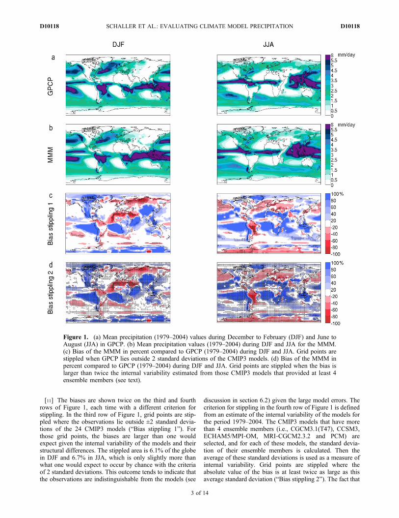
[11] The biases are shown twice on the third and fourthrows of Figure 1, each time with a different criterion forstippling. In the third row of Figure 1, grid points are stip-pled where the observations lie outside ±2 standard devia-tions of the 24 CMIP3 models (“Bias stippling 1”). Forthose grid points, the biases are larger than one wouldexpect given the internal variability of the models and theirstructural differences. The stippled area is 6.1% of the globein DJF and 6.7% in JJA, which is only slightly more thanwhat one would expect to occur by chance with the criteriaof 2 standard deviations. This outcome tends to indicate thatthe observations are indistinguishable from the models (see

discussion in section 6.2) given the large model errors. Thecriterion for stippling in the fourth row of Figure 1 is definedfrom an estimate of the internal variability of the models forthe period 1979–2004. The CMIP3 models that have morethan 4 ensemble members (i.e., CGCM3.1(T47), CCSM3,ECHAM5/MPI‐OM, MRI‐CGCM2.3.2 and PCM) areselected, and for each of these models, the standard devia-tion of their ensemble members is calculated. Then theaverage of these standard deviations is used as a measure ofinternal variability. Grid points are stippled where theabsolute value of the bias is at least twice as large as thisaverage standard deviation (“Bias stippling 2”). The fact that

Figure 1. (a) Mean precipitation (1979–2004) values during December to February (DJF) and June toAugust (JJA) in GPCP. (b) Mean precipitation values (1979–2004) during DJF and JJA for the MMM.(c) Bias of the MMM in percent compared to GPCP (1979–2004) during DJF and JJA. Grid points arestippled when GPCP lies outside 2 standard deviations of the CMIP3 models. (d) Bias of the MMM inpercent compared to GPCP (1979–2004) during DJF and JJA. Grid points are stippled when the bias islarger than twice the internal variability estimated from those CMIP3 models that provided at least 4ensemble members (see text).


3 of 14

72.5% in DJF and 82.6% in JJA of the whole globe isstippled according to this criterion implies that the observa-tions are inconsistent in many areas with respect to themodeled range of natural internal variability, either becauseof observational errors, model errors or because the modelsunderestimate internal variability.[12] The observed and modeled precipitation trends for

the observation period (1980–2004) as well as the modeledprecipitation trends for a 100 year time period in the future(2000–2099) are represented in Figure 2. In the observations(GPCP), many small‐scale structures in the trends can beseen and finding a physical explanation for them is notobvious. Significant drying (at the 95% confidence level)seems to dominate in the polar regions as well as over thewest coasts of the continents while significant wettening ismostly located over Greenland, the Northern Territories andin the Indian ocean. The trends of the MMM from 1980 to

2004 are shown in Figure 2 (middle). If 18 out of the 24CMIP3 models agree on the sign of significant change, thegrid point is stippled, which is never the case during theobservation period. On the one hand, this criterion mini-mizes the possibility that models have the same sign of thetrend just by chance and on the other hand, it is not toostringent to prevent that the criterion is never met, whichwould not be very informative in the case of future trends.For the MMM, a weak wettening of the high latitudes andthe equatorial region can be recognized, while some regionsin the midlatitudes experience a slight drying but thesefeatures are not robustly simulated by the models. Again, thetrends in precipitation of the MMM are not expected toagree perfectly with the trends of GPCP for the same rea-sons described above. The amplitude in the trend patterns issmaller for the MMM than in the observations due to thefact that natural variability is reduced in the MMM because

Figure 2. (top) Precipitation trends (1980–2004) during December to February (DJF) and June toAugust (JJA) in GPCP. Grid points are stippled when the trends are significant at the 95% confidencelevel. (middle) Precipitation trends (1980–2004) during DJF and JJA for the MMM. (bottom) Precipita-tion trends (2000–2099) during DJF and JJA for the MMM. For MMM panels, grid points are stippled ifat least 18 out of 24 models agree on a significant trend (95% confidence level) with the same sign. Notethat the variability in the MMM panels is strongly reduced compared to observations due to the averagingof many ensemble members.


4 of 14

of model averaging [Räisänen, 2007]. Possible reasons for adiscrepancy between observed and modeled precipitationtrends can be many fold: low signal‐to‐noise ratio, obser-vation uncertainties, inadequate parameterizations in themodels as well as incomplete representation of the forcingsor too low spatial resolution. In addition, it must be stressedthat the precipitation trends are nonsignificant in manyregions for GPCP and the CMIP3 models, which indicatesthat at such short time scales, natural variability dominates.[13] For the future time period, a wettening of the high

latitudes and of the equatorial region, along with a drying ofthe midlatitudes can be recognized. Model agreement(stippling if 18 out of the 24 CMIP3 models agree on thesign of significant change) is generally confined to the highlatitudes during the cold season. It is further interesting tonote that the drying is a less robust feature than the wet-tening. The agreement criterion is rarely reached in regionswere a drying is expected because there, variability is largeand mean precipitation low which leads to highly variable

percentage changes in the CMIP3 models. However, thechosen agreement criterion is severe, and robust precipita-tion changes can still be expected in areas where there is nostippling in the bottom row of Figure 2 [see Meehl et al.,2007b, Figure 10.9] as an alternative criterion for modelagreement).

4. Model Agreement

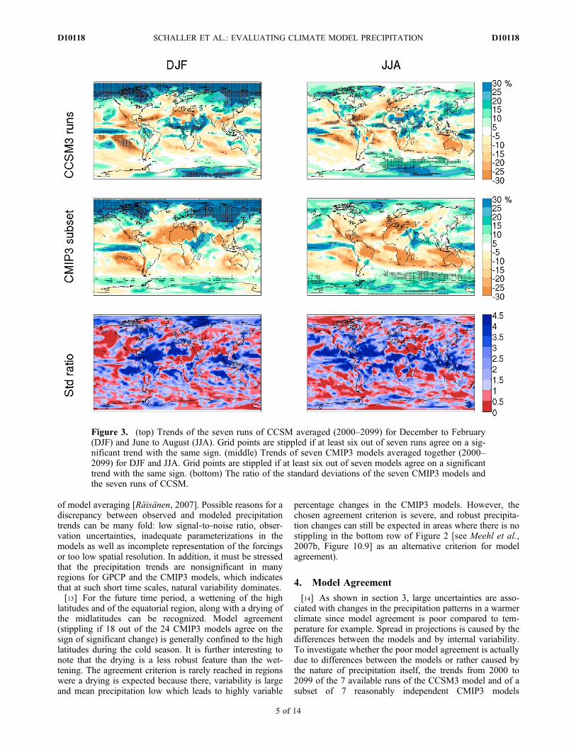
[14] As shown in section 3, large uncertainties are asso-ciated with changes in the precipitation patterns in a warmerclimate since model agreement is poor compared to tem-perature for example. Spread in projections is caused by thedifferences between the models and by internal variability.To investigate whether the poor model agreement is actuallydue to differences between the models or rather caused bythe nature of precipitation itself, the trends from 2000 to2099 of the 7 available runs of the CCSM3 model and of asubset of 7 reasonably independent CMIP3 models

Figure 3. (top) Trends of the seven runs of CCSM averaged (2000–2099) for December to February(DJF) and June to August (JJA). Grid points are stippled if at least six out of seven runs agree on a sig-nificant trend with the same sign. (middle) Trends of seven CMIP3 models averaged together (2000–2099) for DJF and JJA. Grid points are stippled if at least six out of seven models agree on a significanttrend with the same sign. (bottom) The ratio of the standard deviations of the seven CMIP3 models andthe seven runs of CCSM.


5 of 14

(CGCM3.1(T47), CSIRO‐Mk3.5,GFDL‐CM2.1, INGV‐SXG,MIROC3.2(medres), ECHAM5/MPI‐OM, MRI‐CGCM2.3.2)are computed (see Figure 3). The conclusions however donot depend on the exact choice of the subset but likely holdfor all possible subsets. While the exact location of spatialpatterns of significant precipitation change are slightly dif-ferent between the 7 CCSM3 runs and the 7 CMIP3 models,the wettening of the high latitudes and the equatorialregion along with drying in some areas in the midlatitudesare captured by both. Again, a model agreement criterion isdefined: grid points are stippled if at least 6 out of 7 runs/models agree on a significant sign of change. The percentageof area stippled is larger in the 7 CCSM3 runs (13.6% in DJFand 11.8% in JJA) compared to the 7 CMIP3 models (9% inDJF and 5.8% in JJA), as can be expected. Nevertheless, thearea stippled for the 7 CCSM3 runs is surprisingly small andstill in the same range as for the 7 CMIP3 models. This resultindicates that even if the uncertainty caused by model dif-ferences is eliminated, internal variability still contributesstrongly to the lack of agreement in precipitation projections.[15] The relative importance of internal variability com-

pared to model differences can be further quantified. Theratio of the standard deviations of the CMIP3 subset com-pared to the CCSM runs is computed in Figure 3 (bottom).The global average of this ratio is roughly 3 (2.7 in DJF and2.95 in JJA), meaning that the contribution of model dif-ferences is around 3 times larger than that of internal vari-ability in terms of standard variation.Whilemodel differencesdominate, this does not imply that reducing model uncer-tainty in future projections will necessarily improve thesignificance of the projected trends. For single grid pointswhere variability is large, the signal may not be significanteven in a perfect model.

5. Ranking

5.1. Method

[16] In this section, the climate models are evaluated on aregional scale using feature‐based metrics. These metrics aredesigned to focus on areas that reveal a clear signal ofchange in precipitation over the time period considered. Thishas also been the motivation, at least to some extent, ofprevious studies [Pitman et al., 2004; Pierce et al., 2009;Perkins and Pitman, 2009] but with the difference that theyconcentrated only on one region of interest. Here the aimis to go one step further by defining metrics in differentregions of the globe over land and ocean parts and tocompare the performance of the individual models usingseveral feature‐based metrics.

[17] The selected features are regions where the predictedprecipitation change is robust. They are identified with themap of the future trends in precipitation of the MMM dis-cussed in section 4 for two different seasons (DJF and JJA;see Figure 2, bottom). Eight metrics, which we refer to asprecipitation indices (see Table 1 for definitions) are chosen,based on the significance of the trends and on the scientificunderstanding of the physical processes responsible forthese changes. It is important to emphasize that the eightprecipitation indices have to be regarded as examples andnot as the only set of feature‐based metrics possible.[18] The eight precipitation indices are defined in Table 1.

The storm tracks index (STI) is designed to detect thepoleward shift of the storm tracks in the Southern Hemi-sphere, where zone A refers to the preferred region ofcyclone activity in the past and zone B to the region wherethe storms are expected to pass by in the future [Hoskins andHodges, 2005; Previdi and Liepert, 2007]. The Africanindex (AFI) and the Australian index (AUI) capture theprecipitation decrease over the midlatitudes of the SouthernHemisphere that are related to the positive trend of theSouthern Annular Mode (SAM) index prevailing since theclimate shift of the mid‐1970s [Thompson and Solomon,2002]. The Asian index (ASI) depicts the expecteddecrease of precipitation during the dry season and theincrease of precipitation during the wet season in SoutheastAsia. In the context of global warming, more warming overland than over the ocean is expected leading to a northwardshift of the lower tropospheric monsoon circulation andconsequently to an increase in mean precipitation during theAsian summer monsoon [Dairaku and Emori, 2006; Sunand Ding, 2010]. Changes in the location of the ITCZ arealso expected to reduce precipitation during June, July andAugust (JJA) over the Amazon Basin (the Amazonianindex, AMI) [Christensen et al., 2007]. For the NorthernHemisphere, the high‐latitudes index (HLI) captures theincrease in precipitation during December, January andFebruary (DJF) over the continents [Previdi and Liepert,2007]. In a warmer climate moisture convergence towardthe convection zones will increase and as a consequence,moisture divergence in the midlatitudes will be enhanced,causing a decrease in precipitation [Neelin et al., 2006]. Themost prominent features of this subtropical/lower midlati-tude drying in the Northern hemisphere are the JJA pre-cipitation decrease over the Caribbean/Central Americanregion (captured by the Central American index, CAI) andthe one over the Mediterranean region captured by theMediterranean index (MEI), which is also associated withthe soil moisture feedback over land [Rowell and Jones,2006; Seneviratne et al., 2006].

Table 1. Definition of the Precipitation Indicesa

Index Name Definition Domain

African index AFI = PrJJA 13°S–35°S, 14°E–42°EAmazonian index AMI = PrJJA 24°S–1°N, 31°W–59°W, land onlyAsian index ASI = PrJJA ‐ PrDJF 10°N–29°N, 70°E–118°EAustralian index AUI = PrJJA 10°S–40°S, 107°E–138°ECentral American index CAI = PrJJA 10°N–29°N, 110°W–62°WHigh‐latitudes index HLI = PrDJF 52°N–71°N, land onlyMediterranean index MEI = PrJJA 29°N–49°N, 11°W–37°EStorm tracks index STI = PrDJFB ‐ PrDJFA zone A (35°S–46°S)/zone B (49°S–60°S)

aPrDJF (PrJJA) denotes the mean precipitation during DJF (JJA) in the corresponding domain.


6 of 14

[19] Due to the heterogeneity of primary data, the qualityof the merged gauge‐satellite monthly precipitation pro-ducts, GPCP and CMAP, cannot be expected to be equallygood in the 8 regions where the feature‐based metrics aredefined. In general, GPCP and CMAP are more similar overland than over oceans, simply due to the availability ofgauge measurements [Yin et al., 2004]. Consequently, thequality of the observation data sets is expected to be betterfor precipitation indices defined mainly over land, like theAFI, AMI AUI and MEI. As can be seen on Figure 5, GPCPis slightly different from CMAP for the ASI and CAI sincethese indices are mainly defined over oceans. The largestdifferences between both data set are however encounteredfor the two metrics defined in the high latitudes, hence theHLI and STI, where both data sets use different input data[Yin et al., 2004]. Despite the inherent uncertainties, theGPCP and CMAP data sets can be regarded as best estimatedata sets of precipitation patterns.[20] The precipitation indices allow to identify whether

some models clearly perform better than average in regionswhere significant changes are expected and where thephysical processes responsible for the changes are thoughtto be understood. The spatial pattern of precipitation withina region is however not evaluated. It is further interesting toinvestigate if the good models in a given region also performwell in this region but for another variable [Whetton et al.,2007]. We therefore compare the results obtained for pre-cipitation with temperature. Temperature is chosen becauseits signal of change does not strongly depend on the regionconsidered and the field is relatively homogeneous. For thisreason, temperature indices can be defined in the sameregion and for the same season as the precipitation indicesand still be meaningful. The ASI and STI are exceptionsbecause they describe processes that exist for precipitationbut not for temperature. The ASI and STI for temperatureare therefore simply defined as a temperature average forone season (see Table 2).[21] The eight index trends of the MMM from 1980 to

2079 are significant on the 0.01 level for both variables.Unfortunately, the observational period is short and in caseof precipitation, trends are not significant as discussed insection 3, making an evaluation of the trends meaningless.Consequently, the CMIP3 models and the MMM are rankedaccording to their ability to simulate the mean value of eachindex during the observation period (precipitation indexranking and temperature index ranking hereafter). The errorsof each model at simulating the mean index value are simplycalculated as difference between the observed index mean

and the modeled index mean and do not include informationabout discrepancies in the spatial structure within the indexdomain. To compare and aggregate these performancemetrics, they are converted to a common ranking system. Arank of 1 is attributed to the model with the smallest error onthe metric considered, a rank of 2 to the second‐best model,etc. While some quantitative information is lost in thisranking method, it has the advantage that indices with dif-ferent scales and units can readily be compared in anaggregated form. Finally, to summarize the performances ofthe models over the eight indices, the ranks obtained foreach of the eight indices are summed up, and this sum isranked again (lines “Prec ALL” and “Temp ALL” inFigure 4). The sum of the ranks for the precipitation indicesand the temperature indices is finally ranked in Figure 4c(“indices”). The motivation for summing the ranks overdifferent regions and variables is to test if the index‐basedresults gradually converge to the widely used broad‐brushmetrics that summarize performances for a large range ofclimate variables on a global scale.[22] The index ranking is first compared to a ranking

performed on global scale, again for both variables, pre-cipitation and temperature, only. The root mean square error(rmse) of each model with respect to the observations andthe spatial correlation between simulated and observedprecipitation and temperature (referred to as the rmse/corrranking hereafter) are calculated separately for each vari-able. The model having the lowest rmse (highest correlationcoefficient) ranks first. In Figure 4c, the “rmse/corr” depictsa ranking of the sum of the ranks obtained for both variableson the rmse and the corr ranking, again to identify if bydoing so, the outcomes of the broad‐brush metrics can bereproduced.[23] Finally, the index and the rmse/corr rankings are

compared to a ranking performed with a broad‐brush metric,which is a version of the ranking on a broad range of climatevariables performed by Reichler and Kim [2008] (RK08ranking hereafter), updated with more variables and usingfour seasons (T. Reichler, personal communication, 2009).[24] In summary, the RK08 ranking identifies the model

performance on a global scale summarized for differentclimate variables, the rmse/corr ranking provides a pictureof the models’ spatial error with respect to the precipitationand temperature data on a global scale and the index rankingallows for the identification of the models that best simulatelocal precipitation and temperature features expected tochange in the future due to anthropogenic forcing.

5.2. Results and Discussion

[25] The results of the index rankings for both precipita-tion and temperature are summarized in Figure 4a. At firstglance, none of the CMIP3 models appears to consistentlyoutperform the rest. This is particularly obvious in the pre-cipitation index ranking. Here, each model performs at leastonce better and worse than the average, while the MMMperforms average for all indices. The results for the tem-perature index ranking are only slightly different: again themodels can perform better and worse than average for dif-ferent indices, except ECHAM5/MPI‐OM and the MMM,which always perform better than average. It is furtherinteresting to note that there are no significant correlationsamong the eight indices for each variable nor between

Table 2. Definition of the Temperature Indicesa

Index Name Definition Domain

African index AFI = T JJA 13°S–35°S, 14°E–42°EAmazonian index AMI = T JJA 24°S–1°N, 31°W–59°W,

land onlyAsian index ASI = T JJA 10°N–29°N, 70°E–118°EAustralian index AUI = T JJA 10°S–40°S, 107°E–138°ECentral American index CAI = T JJA 10°N–29°N, 110°W–62°WHigh‐latitudes index HLI = TDJF 52°N–71°N, land onlyMediterranean index MEI = T JJA 29°N–49°N, 11°W–37°EStorm tracks index STI = TDJFAB zone AB (35°S–60°S)

aTDJF (T JJA) denotes the mean temperature during DJF (JJA) in thecorresponding domain.


7 of 14

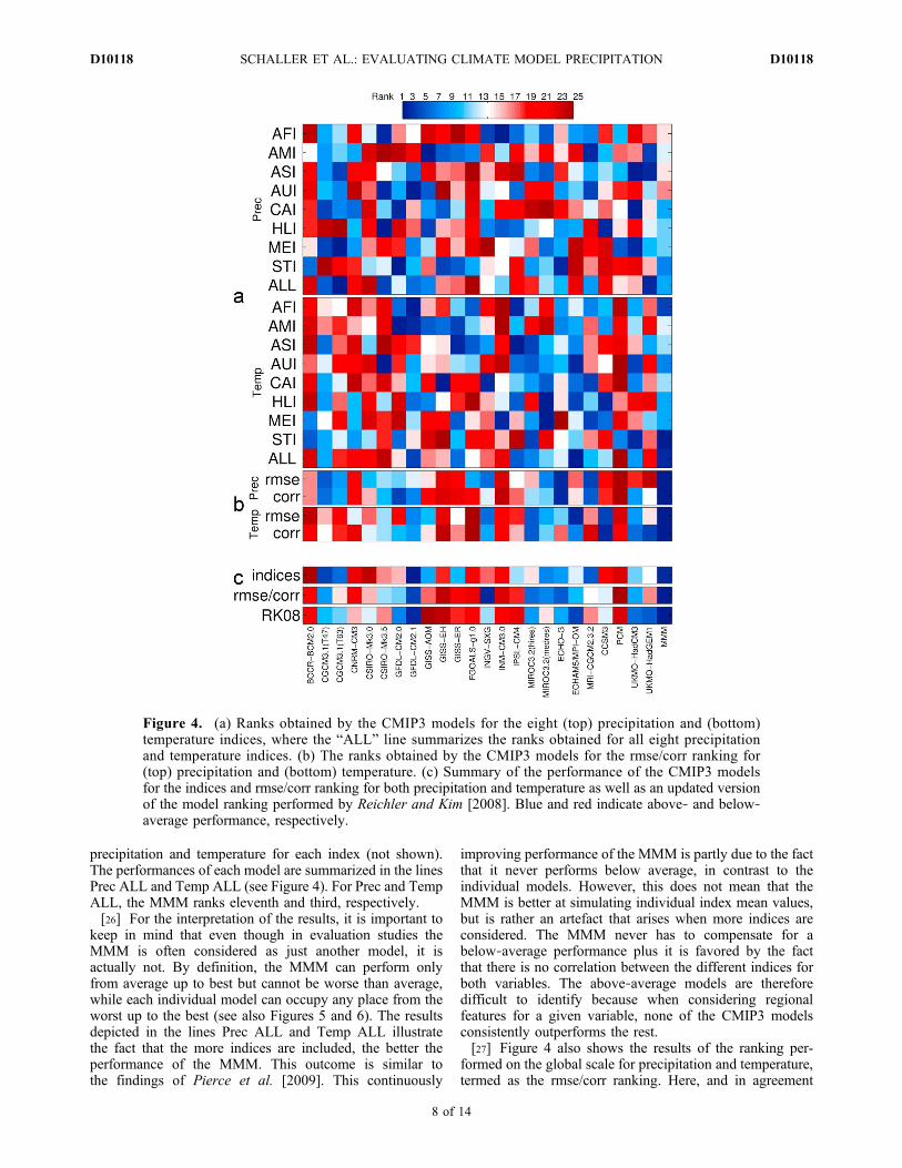
precipitation and temperature for each index (not shown).The performances of each model are summarized in the linesPrec ALL and Temp ALL (see Figure 4). For Prec and TempALL, the MMM ranks eleventh and third, respectively.[26] For the interpretation of the results, it is important to

keep in mind that even though in evaluation studies theMMM is often considered as just another model, it isactually not. By definition, the MMM can perform onlyfrom average up to best but cannot be worse than average,while each individual model can occupy any place from theworst up to the best (see also Figures 5 and 6). The resultsdepicted in the lines Prec ALL and Temp ALL illustratethe fact that the more indices are included, the better theperformance of the MMM. This outcome is similar tothe findings of Pierce et al. [2009]. This continuously

improving performance of the MMM is partly due to the factthat it never performs below average, in contrast to theindividual models. However, this does not mean that theMMM is better at simulating individual index mean values,but is rather an artefact that arises when more indices areconsidered. The MMM never has to compensate for abelow‐average performance plus it is favored by the factthat there is no correlation between the different indices forboth variables. The above‐average models are thereforedifficult to identify because when considering regionalfeatures for a given variable, none of the CMIP3 modelsconsistently outperforms the rest.[27] Figure 4 also shows the results of the ranking per-

formed on the global scale for precipitation and temperature,termed as the rmse/corr ranking. Here, and in agreement

Figure 4. (a) Ranks obtained by the CMIP3 models for the eight (top) precipitation and (bottom)temperature indices, where the “ALL” line summarizes the ranks obtained for all eight precipitationand temperature indices. (b) The ranks obtained by the CMIP3 models for the rmse/corr ranking for(top) precipitation and (bottom) temperature. (c) Summary of the performance of the CMIP3 modelsfor the indices and rmse/corr ranking for both precipitation and temperature as well as an updated versionof the model ranking performed by Reichler and Kim [2008]. Blue and red indicate above‐ and below‐average performance, respectively.


8 of 14

with previous studies [Phillips and Gleckler, 2006; Gleckleret al., 2008; Pincus et al., 2008], the MMM clearly performsbest for both variables. Averaging the individual modelssmoothes out variations and small‐scale biases of the pre-cipitation field, so that errors partly cancel out in the MMM[Phillips and Gleckler, 2006; Pierce et al., 2009]. Conse-quently, the MMM is favored by global statistical metricsbecause of its relatively small magnitude of biases over thewhole globe and its good representation of the spatial pat-tern, while feature‐based metrics favor a single modelcapable of displaying the area mean precipitation over a

given region. Except for the performance of the MMM,the rmse/corr ranking is quite different for precipitationand temperature, illustrating that also globally, a modelperforming well for a variable might perform poorly for another. Further, it is interesting to compare the index rankingwith the rmse/corr ranking for each variable individually.The Spearman’s rank correlation coefficient between PrecALL and Prec rmse is nonsignificant at the 95% level whileit is significant between Prec ALL and Prec corr (r = 0.49).For temperature, the correlations are also low but signifi-cant: r = 0.56 between Temp ALL and Temp rmse and

Figure 5. (a–h) (left) Time series and (right) anomalies relative to the observational period of the CMIP3models, CMAP, and GPCP for the eight precipitation indices. The five best models for each index aregiven as dark blue lines, while the black line represents the MMM. An 11 year average is applied tothe time series. The mean value and ±1 standard deviation in the year 2079 are shown in light blue (darkblue) for all CMIP3 models (five best models).


9 of 14

r = 0.4 between Temp ALL and Temp corr. This indicatesthat when the performances of the individual models on afew chosen regional features are summarized, the results of aranking based on the rmse or correlation on a global scalecan be approached.[28] Finally, the errors obtained for all precipitation and

temperature indices are summed to obtain the line “indices” onFigure 4c, which can be compared with the rmse/corr rankingand the broad‐brush metric ranking RK08 (Figure 4c). Inthis final index ranking, the MMM ranks fifth and it isreasonable to assume that including more regional features

and/or more variables will contribute to improve the rank ofthe MMM, which will eventually rank first. It is obvious thatthe MMM ranks first for the rmse/cor ranking since it wasalready the case for the rmse and corr ranking of eachindividual variable. The MMM also ranks first in the RK08ranking for the same reason. By definition the error of theMMM at each grid point cannot be larger than the meanerror of the models and consequently, the errors of theMMM are the smallest when averaged globally. Neverthe-less, the three ways of ranking presented here share simi-larities. The Spearman’s rank correlations are significant

Figure 6. (a–h) (left) Time series and (right) anomalies relative to the observational period of the CMIP3models and ERA‐40 for the eight temperature indices. The five best models for each index are given asdark blue lines, while the black line represents the MMM. An 11 year average is applied to the time series.The mean value and ±1 standard deviation in the year 2079 are shown in light blue (dark blue) for allCMIP3 models (five best models).


10 of 14

between the three rows in Figure 4c: r = 0.44 between“indices” and “RK08,” r = 0.61 between “indices” and“rmse/corr” and r = 0.78 between “RK08” and “rmse/corr.”This shows that when summarizing the errors at simulatingthe mean of several feature‐based metrics for differentvariables, the performance of the individual models is partlythe same as when evaluating the models with measures ofthe global spatial distribution and including more (e.g.,RK08 ranking) or less (e.g., rmse/corr ranking) climatevariables.[29] To summarize, an evaluation of the models using

global statistical measures like the RK08 ranking does notcapture the average performance of the MMM at simulatingthe mean precipitation amounts in a given region. Suchevaluation techniques rather reflect the fact that the MMMhas the smallest errors as soon as the domain size exceedsseveral grid points because it cannot have per definition themaximal error on a grid point (in contrary to the individualmodels). When the ranks obtained for the eight precipitationand temperature indices are summed up and ranked again, asimilar result is seen: the MMM does not have to com-pensate for poor rankings and the performance of the MMMbecomes gradually better the more regions and variables aresummed up. The information that single models are betterthan the MMM at simulating regional mean precipitationamounts for a given season can be relevant for impactstudies but is hidden in evaluations using a global broad‐brush approach. In addition, the results obtained for tem-perature suggests that the worse performance of the MMMfor the feature‐based metrics compared to global summarystatistics is not a particularity of precipitation but is likely tohold for most variables. The interpretation of the MMM isfurther discussed at the end of section 6.

6. Future Projections

6.1. Method

[30] Once the models performing best for a given regionalfeature are identified, the question arises whether thesemodels will still be the best performing ones in the future.The assumption that the models simulating the present cli-mate accurately will also simulate well the future climate isoften made [e.g., Tebaldi et al., 2004]. While it is impos-sible for obvious reasons to perform a model evaluationwith feature‐based metrics for the future to check if thisassumption is correct, investigating the convergence of themodels on future predictions can partly answer this ques-tion. If a subset of models (chosen based on agreement withobservations) shows considerably smaller spread, then theobservations can be regarded as useful to distinguishbetween models. This is equivalent to a correlation betweenbiases in the present‐day simulation and the predictedchange. The assumption is that such correlation is not just anartifact of all models making similar assumptions, but ratherthat it reflects an underlying physical process or feedbackthat influences both the base state of a model as well as thesimulated change. In practice such correlations unfortu-nately are relatively low in many cases [Knutti et al., 2010b;Whetton et al., 2007], probably partly as a consequence ofthe observations being used already in the model develop-ment process.

[31] The time evolution of the absolute values and theanomalies of the eight precipitation and temperature indicesfor the 100 year period 1980–2079 is shown in Figures 5and 6 using an 11 year average. For the precipitation indi-ces, the time series of GPCP and CMAP for 1980–2004 arealso presented. Similarly, the index time series of ERA‐40are shown besides the modeled index time series of tem-perature. In addition, for each variable and each index, thefive models performing best are identified and representedby dark blue lines. The model spread by the end of 2079 forall models and the five best models is represented by anerror bar at the right of each panel. The error bars representthe mean value ±1 standard deviation.

6.2. Results and Discussion

[32] Figure 5 shows the modeled absolute and anomalytime series of each precipitation index from 1980–2079along with the observed absolute and anomaly time seriesfrom 1980–2004. The model spread is large for all indices.For example, in case of the absolute values of the ASI, theprojections vary by a factor of 5, hence the difficulty to giveclear statements about future precipitation amounts in thisregion. The reason for the average performance of theMMM in the index ranking presented above becomes evi-dent by looking at the time series. The MMM by definitionlies in the middle of the model spread, while the observationdata sets lie in most indices at one end of the model spread.Many models have similar biases and averaging modelstherefore does not reduce the biases, which explains why theMMM cannot perform best. In addition, the individualmodels capture better the natural variability of regionalprecipitation patterns than the MMM. This is due to the factthat by averaging all 24 CMIP3 models to construct theMMM, natural variability is automatically removed.[33] As already mentioned, regional trends over the rela-

tively short observational period (25 years) are often dom-inated by natural variability which is why the evaluation isonly performed on the ability of the models to simulate theindex mean value. Still, it is central that climate models areable to correctly simulate the trends. A source of concern inthe case of the HLI is the inability of most CMIP3 models toreproduce the DJF precipitation decrease during the obser-vational period. Further, the discrepancies between the twoobservational data sets CMAP and GPCP are very large forthe HLI and STI. While for the rmse/corr ranking thesedifferences have only a marginal influence (not shown),using CMAP as the reference data set for the feature‐basedranking described above will lead to different outcomes. Incertain regions it is therefore currently ambiguous to identifythe best models due partly to uncertainties in the observa-tional data sets. The implication is that the difficulties indefining model performance are not only a problem ofagreeing on a metric, but is seriously limited by observationaluncertainties. This underscores the need for continuous,global and homogeneous observations at high resolution.[34] Considering only the five best models for each index

narrows the range of predicted absolute values (dark bluelines in Figure 5), as expected. However, if anomalies areconsidered (see right‐hand plots in Figures 5a–5h), themodel spread is only reduced for 3 indices (AFI, HLI andSTI; see error bars in Figure 5), it remains approximately thesame for the AUI and CAI and even increases for the AMI,


11 of 14

ASI and MEI. The results of the temperature index timeseries are shown on Figure 6. In contrast to precipitation, thesignal of temperature change dominates the natural vari-ability and model agreement is larger. However, in terms ofanomalies, only a minority of indices (AMI and HLI) see areduction of model spread.[35] The way the MMM was calculated in this study can

be referred to as an “equal weighting” because each modelhas one “vote.” A more sophisticated approach consists inassigning more weight to the “good” models. Severalstudies see some improvement in future projections whenusing “optimum weighting” approaches [e.g., Perkins andPitman, 2009; Räisänen et al., 2010]. On the other hand,Santer et al. [2009] find that an “optimum weighting” doesnot affect the results of their detection and attribution studyfor water vapor. For the feature‐based metrics presentedhere, applying an “optimum weighting” to the modelsaccording to the ranking presented in section 6.1 will likelylead to a reduction of the uncertainty for only a few indicesbut these indices are different for precipitation (AFI, HLIand STI) and temperature (AMI and HLI). However, theproblem is that an “optimum weighting” would keep themodel uncertainty constant or even increase it for the rest ofthe indices. In addition, the differences in model spreadfound between the five best models and all models arehighly time dependent: calculating the standard deviation bythe year 2059 or 2099 would have lead to slightly differentoutcomes in terms of the indices showing a reduction ofspread but the conclusion would remain the same. A furthercritical issue is the sampling of small subsets. The standarddeviation may also change by picking a random subset ofthe models, even if the criteria for picking the models has norelevance at all. For 5 out of 24 models, there is a proba-bility of about 5% for the spread (standard deviation) toincrease or decrease by 50% or more in a random subset. Inother words, at least a 50% change in the spread can beconsidered significant and very unlikely to arise by chance.Only the AFI for precipitation and the HLI for temperatureshow such large changes. In most indices the change in thespread after selecting the subset of models is well withinwhat one would expect from randomly picking a subset. Theresults presented here are in agreement with Weigel et al.[2010], who argued that even if for some cases the “opti-mum weighting” outperforms the “equal weighting,” therisk that the former is worse than the latter is large. In caseswhere there is currently no agreement on which skill mea-sure to use in order to identify the best models, it is indeedmore transparent to weight the models equally. However,Weigel et al. [2010] also showed that not considering thosemodels known for lacking key mechanisms needed to pro-vide meaningful projections might be justified in somecases.[36] Further, Knutti et al. [2010b] showed that means and

trends are generally not well correlated. In the case of theprecipitation indices, a significant Pearson correlationcoefficient between index mean (1980–2004) and trend(2020–2079) is only found for the STI (r = −0.43), an indexfor which the model uncertainty is reduced when consider-ing only the five best models. For the temperature indices, asignificant correlation is found for the ASI (r = 0.43) andthe CAI (r = 0.48), which are indices that do not experiencereduction of model spread when selecting only the five best

models. However, given that these correlations are low andthat there is no obvious physical explanation for them, theyshould not be overinterpreted. Rather, the fact that signifi-cant correlations between means and trends for an index donot always correspond to those indices with a reductionof model spread when considering the five best modelsindicates that feature‐based metrics are not more useful toreduce the uncertainty in terms of anomalies than othermetrics. Nevertheless, many end users are interested inabsolute precipitation amounts and in this case, feature‐based metrics are a simple way to identify the models thathave some skill in a region but also to identify those whohave obviously no skill.[37] Finally, it should be noted that the interpretation of

the MMM has been the subject of some debate. In particular,different interpretations of model independence, modelrobustness and of the ensemble of models itself are possibleand lead to different interpretations of future model uncer-tainty [Pirtle et al., 2010; Knutti et al., 2010b, 2010a; Annanand Hargreaves, 2010]. On the one hand, climate modelscan be considered as “random samples from a distribution ofpossible models centered around the true climate” [Jun et al.,2008]. Consequently, when averaging all models to constructthe MMM, the errors are expected to decrease and the MMMto approach the truth [Tebaldi et al., 2004]. The statisticallyindistinguishable ensemble paradigm is an alternative way tointerpret ensembles, where the truth is a sample from thesame distribution as each model of the ensemble [e.g.,Tebaldi and Sanso, 2009]. Annan and Hargreaves [2010]compared both paradigms and find that the CMIP3 ensem-ble generally provides a good sample under the statisticallyindistinguishable paradigm. Assessing the statistical natureof the CMIP3 ensemble is beyond the scope of this studyhowever, results from section 3 as well as in the case of theeight feature‐based metrics for precipitation, it seems thatthe ensemble of models is not centered around the truth butappears biased. Therefore, the MMM is not closer than anyother model to the observations, which seem to be statisti-cally indistinguishable from the ensemble members. Fortemperature, the CMIP3 ensemble also appears biased but toa smaller extent than for precipitation. Nevertheless, thereis a need for further studies focusing on how to interpretresults from multiple models.

7. Conclusion

[38] The motivation for ranking the models is to specifywhich one(s) can provide the most reliable projections. Untilnow, model simulations have often been evaluated withstatistical measures and on large spatial scales, where theMMM was found to perform best. As an alternative evalu-ation method, we provide eight feature‐based performancemetrics for precipitation and temperature. Feature‐basedmetrics are designed to capture a robust signal of change in aparticular variable that can be explained physically. As afirst step, the causes behind the large projection uncertaintyfor precipitation are investigated. In large regions of theworld, differences between the models contribute more tothe total spread in projections than internal variability.However, agreement in the sign of trend among several runsof the same model is only slightly larger than among dif-ferent models, indicating that even if differences between


12 of 14

models are reduced, internal variability will still cause alarge lack of agreement in precipitation projections.[39] For the regional feature‐based metrics, the models

performing best are different for each region and variable,and the choice of the observational data set is important inthe case of precipitation. Averaging the models is moreeffective on aggregated metrics than on small scales andfeatures. This is illustrated by the fact that when summa-rizing the performances of the models for all indices andboth variables, the MMM ranks better than for each indexindividually. When the performances for the feature‐basedmetrics are summarized, they correlate with the rankingobtained with statistical measures of errors and with theglobal field‐based measures of Reichler and Kim [2008].This is agreement with earlier studies [Boer, 1993; Gleckleret al., 2008; Pincus et al., 2008] who find that the MMMoutperforms any individual model if enough metrics or gridpoints are evaluated and aggregated. We also tested a furtherway of ranking the models based on their ability to simulatethe spatial correlation between the mean precipitation andtemperature pattern in the index regions (not shown). It wasfound that the performance of the MMM for this regionalcorrelation ranking is between its performance in the indexranking and the corr ranking for both precipitation andtemperature. The MMM ranked first in ∼35% of the cases,which is better than for the index ranking where it ranksaverage, but worse than for the corr ranking where it clearlyranks first. These findings confirm our hypothesis that themore grid cells, metrics or variables are aggregated, thebetter the performance of the MMM becomes.[40] In a second part, the convergence of the projections

of the best performing models for each index is investigated.On one hand and in particular for precipitation, the projec-tions of the five best models in terms of absolute valuesappear more realistic than the ones performing belowaverage since for most indices, the observations lie at oneend of the model spread. However, when considering theanomalies, it is found that regardless of the variable, themajority of the indices see no reduction or even an increasein future uncertainty. These results suggest that on a regionalscale, weighting the models might improve the projectionsonly in few cases. In the absence of a process based argu-ment, given the small number of existing models and thechosen subsets of 5 models, only a reduction in modelspread by more than 50% is an indication of a successfulconstraint (see section 6.2). Model weighting should there-fore be performed carefully. Our results tend to supportprevious findings showing that a good performance in thepresent does not guarantee skill in the future [Jun et al.,2008; Reifen and Toumi, 2009]. On the other hand, thereare a few cases where past and future performance in modelsare clearly related and physically well understood, forexample, past greenhouse gas attributable warming scalinglinearly with future transient greenhouse gas warming [Allenand Ingram, 2002; Stott et al., 2006]. Such relationships areroutinely used and widely accepted to constrain or calibrateprojections with simple and intermediate complexity models[e.g., Knutti et al., 2002; Forest et al., 2002; Meinshausenet al., 2009]. Another prominent example is the Arctic,where models underestimating past sea ice decline alsoshow much weaker sea ice loss in the future [Boe et al.,2009b] and where performance in simulating the current

Arctic climate is related to projected future response in thatregion [Boe et al., 2009a; Mahlstein and Knutti, 2011]. Insuch obvious cases we argue that observed evidence shouldnot be ignored when synthesizing models.[41] Evaluating the models is a central task in climate

science and the reason why there is currently no agreementon a standard way to perform an evaluation reflects the factthat on the one hand, the connection between present‐dayand future performance is poorly understood and on theother hand, it also depends on the purpose. While hydrol-ogists need assessments of the best performing models on aregional scale and primarily for precipitation and tempera-ture, some model developers are more interested in sum-marizing the performance of climate models for manyvariables and over all regions of the globe as for example inwork by Reichler and Kim [2008]. For specific applicationsand predictions, defining metrics not only based on meanbiases but also on regional or temporal characteristics (e.g.,distributions of daily rainfall) or on physical processes [e.g.,Eyring et al., 2005] may be more promising. It is evidentthat the index ranking presented here is partly subjective dueto the choice of the eight indices. The indices shouldtherefore be regarded as examples and depending on thepurpose, other sets of indices can be defined. We also pointout that the results are at most valid for precipitation andtemperature and do not allow for any evaluations of themodel performance on other variables or on a global scale.Further considerations of alternative ways of evaluatingclimate models in order to make best use of their predictionsare encouraged.

[42] Acknowledgments. We acknowledge the modeling groups, theProgram for Climate Model Diagnosis and Intercomparison (PCMDI)and the WCRP’s Working Group on Coupled Modeling (WGCM) for theirroles in making available the WCRP CMIP3 multimodel data set. Supportfor this data set is provided by the Office of Science, U.S. Department ofEnergy.

ReferencesAdler, R. F., et al. (2003), The version‐2 global precipitation climatologyproject (GPCP) monthly precipitation analysis (1979–present), J. Hydro-meteorol., 4(6), 1147–1167.

Allen, M. R., and W. J. Ingram (2002), Constraints on future changes inclimate and the hydrologic cycle, Nature, 419, 224–232, doi:10.1038/nature01092.

Annan, J. D., and J. C. Hargreaves (2010), Reliability of the CMIP3 ensem-ble, Geophys. Res. Lett., 37, L02703, doi:10.1029/2009GL041994.

Boe, J., A. Hall, and X. Qu (2009a), Deep ocean heat uptake as a majorsource of spread in transient climate change simulations, Geophys. Res.Lett., 36, L22701, doi:10.1029/2009GL040845.

Boe, J. L., A. Hall, and X. Qu (2009b), September sea‐ice cover in the ArcticOcean projected to vanish by 2100, Nat. Geosci., 2(5), 341–343,doi:10.1038/NGEO467.

Boer, G. J. (1993), Climate change and the regulation of the surface mois-ture and energy budgets, Clim. Dyn., 8(5), 225–239.

Christensen, J., et al. (2007), Regional climate projections, in ClimateChange 2007: The Physical Science Basis. Contribution of WorkingGroup I to the Fourth Assessment Report of the Intergovernmental Panelon Climate Change, edited by S. Solomon et al., pp. 847–940, CambridgeUniv. Press, Cambridge, U. K.

Dairaku, K., and S. Emori (2006), Dynamic and thermodynamic influenceson intensified daily rainfall during the Asian summer monsoon underdoubled atmospheric CO2 conditions, Geophys. Res. Lett., 33, L01704,doi:10.1029/2005GL024754.

Eyring, V., et al. (2005), A strategy for process‐oriented validation ofcoupled chemistry‐climate models, Bull. Am. Meteorol. Soc., 86,1117–1133, doi:10.1175/BAMS-86-8-1117.


13 of 14

Forest, C. E., P. H. Stone, A. P. Sokolov, M. R. Allen, and M. D.Webster (2002), Quantifying uncertainties in climate system propertieswith the use of recent climate observations, Science, 295(5552), 113–117.

Giorgi, F., and L. O. Mearns (2002), Calculation of average, uncertaintyrange, and reliability of regional climate changes from AOGCM simu-lations via the reliability ensemble averaging (REA) method, J. Clim.,15(10), 1141–1158.

Gleckler, P. J., K. E. Taylor, and C. Doutriaux (2008), Performance metricsfor climate models, J. Geophys. Res., 113, D06104, doi:10.1029/2007JD008972.

Hoskins, B. J., and K. I. Hodges (2005), A new perspective on SouthernHemisphere storm tracks, J. Clim., 18(20), 4108–4129.

Intergovernmental Panel on Climate Change (2007), Climate Change 2007:The Physical Science Basis. Contribution of Working Group I to theFourth Assessment Report of the Intergovernmental Panel on ClimateChange, edited by S. Solomon et al., 996 pp., Cambridge Univ. Press,Cambridge, U. K.

Jun, M., R. Knutti, and D. W. Nychka (2008), Spatial analysis to quantifynumerical model bias and dependence: How many climate models arethere?, J. Am. Stat. Assoc. , 103(483), 934–947, doi:10.1198/016214507000001265.

Knutti, R., T. F. Stocker, F. Joos, and G. K. Plattner (2002), Constraints onradiative forcing and future climate change from observations andclimate model ensembles, Nature, 416, 719–723.

Knutti, R., G. Abramowitz,M. Collins, V. Eyring, P. J. Gleckler, B. Hewitson,and L. Mearns (2010a), Good practice guidance paper on assessing andcombining multi model climate projections, in Meeting Report of the Inter-governmental Panel on Climate Change Expert Meeting on Assessing andCombining Multi Model Climate Projections, edited by T. F. Stocker et al.,13 pp., IPCC Working Group I Tech. Supp. Unit, Univ. of Bern, Bern,Switzerland.

Knutti, R., R. Furrer, C. Tebaldi, J. Cermak, and G. A. Meehl (2010b),Challenges in combining projections from multiple climate models,J. Clim., 23(10), 2739–2758.

Lambert, S. J., and G. J. Boer (2001), CMIP1 evaluation and intercompar-ison of coupled climate models, Clim. Dyn., 17(2‐3), 83–106.

Mahlstein, I., and R. Knutti (2011), Ocean heat transport as a cause for modeluncertainty in projected Arctic warming, J. Clim., 24, 1451–1460,doi:10.1175/2010JCLI3713.1.

Meehl, G. A., C. Covey, T. Delworth, M. Latif, B. McAvaney, J. F. B.Mitchell, R. J. Stouffer, and K. E. Taylor (2007a), The WCRP CMIP3multimodel dataset—A new era in climate change research, Bull. Am.Meteorol. Soc., 88, 1383–1394, doi:10.1175/BAMS-88-9-1383.

Meehl, G. A., et al. (2007b), Global climate projections, in Climate Change2007: The Physical Science Basis. Contribution of Working Group I tothe Fourth Assessment Report of the Intergovernmental Panel on ClimateChange, edited by S. Solomon et al., pp. 747–845, Cambridge Univ.Press, Cambridge, U. K.

Meinshausen, M., N. Meinshausen, W. Hare, S. C. B. Raper, K. Frieler,R. Knutti, D. J. Frame, and M. R. Allen (2009), Greenhouse‐gas emissiontargets for limiting global warming to 2 degrees C, Nature, 458, 1158–1162, doi:10.1038/nature08017.

Neelin, J. D., M. Munnich, H. Su, J. E. Meyerson, and C. E. Holloway(2006), Tropical drying trends in global warming models and observa-tions, Proc. Natl. Acad. Sci. U. S. A., 103(16), 6110–6115.

Perkins, S. E., and A. J. Pitman (2009), Do weak AR4 models bias projec-tions of future climate changes over Australia?, Clim. Change, 93(3‐4),527–558, doi:10.1007/s10584-008-9502-1.

Phillips, T. J., and P. J. Gleckler (2006), Evaluation of continental precip-itation in 20th century climate simulations: The utility of multimodel sta-tistics, Water Resour. Res., 42, W03202, doi:10.1029/2005WR004313.

Pierce, D. W., T. P. Barnett, B. D. Santer, and P. J. Gleckler (2009), Select-ing global climate models for regional climate change studies, Proc. Natl.Acad. Sci. U. S. A., 106(21), 8441–8446, doi:10.1073/pnas.0900094106.

Pincus, R., C. P. Batstone, R. J. P. Hofmann, K. E. Taylor, and P. J. Gleckler(2008), Evaluating the present‐day simulation of clouds, precipitation,and radiation in climate models, J. Geophys. Res., 113, D14209,doi:10.1029/2007JD009334.

Pirtle, Z., R. Meyer, and A. Hamilton (2010), What does it mean when cli-mate models agree? A case for assessing independence among generalcirculation models, Environ. Sci. Policy, 13(5), 351–361.

Pitman, A. J., G. T. Narisma, R. A. Pielke, and N. J. Holbrook (2004),Impact of land cover change on the climate of southwest WesternAustralia, J. Geophys. Res., 109, D18109, doi:10.1029/2003JD004347.

Previdi, M., and B. G. Liepert (2007), Annular modes and Hadley cellexpansion under global warming, Geophys. Res. Lett., 34, L22701,doi:10.1029/2007GL031243.

Räisänen, J. (2007), How reliable are climate models?, Tellus, Ser. A, 59(1),2–29.

Räisänen, J., L. Ruokolainen, and J. Ylhäisi (2010), Weighting of modelresults for improving best estimates of climate change, Clim. Dyn.,35(2‐3), 407–422.

Reichler, T., and J. Kim (2008), How well do coupled models simulatetoday’s climate?, Bull. Am. Meteorol. Soc., 89, 303–311, doi:10.1175/BAMS-89-3-303.

Reifen, C., and R. Toumi (2009), Climate projections: Past performance noguarantee of future skill?, Geophys. Res. Lett., 36, L13704, doi:10.1029/2009GL038082.

Rowell, D. P., and R. G. Jones (2006), Causes and uncertainty of futuresummer drying over Europe, Clim. Dyn., 27(2‐3), 281–299.

Santer, B. D., et al. (2009), Incorporating model quality information inclimate change detection and attribution studies, Proc. Natl. Acad. Sci.U. S. A., 106(35), 14,778–14,783, doi:10.1073/pnas.0901736106.

Seneviratne, S. I., D. Lüthi, M. Litschi, and C. Schär (2006), Land‐atmosphere coupling and climate change in Europe, Nature, 443,205–209, doi:10.1038/nature05095.

Smith, I., and E. Chandler (2010), Refining rainfall projections for theMurray Darling Basin of south‐east Australia—The effect of samplingmodel results based on performance, Clim. Change, 102(3‐4), 377–393,doi:10.1007/s10584-009-9757-1.

Stott, P. A., J. F. B. Mitchell, M. R. Allen, T. L. Delworth, J. M. Gregory,G. A. Meehl, and B. D. Santer (2006), Observational constraints on pastattributable warming and predictions of future global warming, J. Clim.,19(13), 3055–3069.

Sun, Y., and Y. H. Ding (2010), A projection of future changes in summer pre-cipitation and monsoon in East Asia, Sci. China Earth Sci., 53(2), 284–300.

Tebaldi, C., and B. Sanso (2009), Joint projections of temperature and pre-cipitation change from multiple climate models: A hierarchical Bayesianapproach, J. R. Stat. Soc., Ser. A, 172, 83–106.

Tebaldi, C., L. O. Mearns, D. Nychka, and R. L. Smith (2004), Regional prob-abilities of precipitation change: A Bayesian analysis of multimodel simula-tions, Geophys. Res. Lett., 31, L24213, doi:10.1029/2004GL021276.

Thompson, D. W. J., and S. Solomon (2002), Interpretation of recentSouthern Hemisphere climate change, Science, 296(5569), 895–899.

Trenberth, K. E., A. G. Dai, R. M. Rasmussen, and D. B. Parsons (2003),The changing character of precipitation, Bull. Am. Meteorol. Soc., 84,1205–1217, doi:10.1175/BAMS-84-9-1205.

Uppala, S. M., et al. (2005), The ERA‐40 re‐analysis, Q. J. R. Meteorol.Soc., 131(612), 2961–3012, doi:10.1256/qj.04.176.

Weigel, A. P., R. Knutti, M. A. Liniger, and C. Appenzeller (2010), Risksof model weighting in multimodel climate projections, J. Clim., 23(15),4175–4191, doi:10.1175/2010JCLI3594.1.

Whetton, P., I. Macadam, J. Bathols, and J. O’Grady (2007), Assessment ofthe use of current climate patterns to evaluate regional enhanced green-house response patterns of climate models, Geophys. Res. Lett., 34,L14701, doi:10.1029/2007GL030025.

Xie, P. P., and P. A. Arkin (1998), Global monthly precipitation estimatesfrom satellite‐observed outgoing longwave radiation, J. Clim., 11(2),137–164.

Yin, X. G., A. Gruber, and P. Arkin (2004), Comparison of the GPCP andCMAP merged gauge‐satellite monthly precipitation products for theperiod 1979–2001, J. Hydrometeorol., 5(6), 1207–1222.

J. Cermak, R. Knutti, I. Mahlstein, and N. Schaller, Institute forAtmospheric and Climate Science, ETH Zurich, Universitätstrasse 16,CH‐8092 Zurich, Switzerland. ([email protected])


14 of 14

analyzing precipitation projections: a comparison of ... · analyzing precipitation projections: a...

Documents