analyzing reaction times - uni-tuebingen.dehbaayen/publications/baayenmilin2010.pdf · analyzing...

Analyzing Reaction Times

R. Harald BAAYENDepartment of Linguistics, University of Alberta, Canada

Petar MILINDepartment of Psychology, University of Novi Sad, Serbia

Laboratory for Experimental Psychology, University of Belgrade, Serbia

Abstract

Reaction times (rts) are an important source of information in experimentalpsychology. Classical methodological considerations pertaining to the sta-tistical analysis of rt data are optimized for analyses of aggregated data,based on subject or item means (c.f., Forster & Dickinson, 1976). Mixed-effects modeling (see, e.g., Baayen, Davidson, & Bates, 2008) does not re-quire prior aggregation and allows the researcher the more ambitious goal ofpredicting individual responses. Mixed-modeling calls for a reconsiderationof the classical methodological strategies for analysing rts. In this study,we argue for empirical flexibility with respect to the choice of transforma-tion for the rts. We advocate minimal a-priori data trimming, combinedwith model criticism. We also show how trial-to-trial, longitudinal depen-dencies between individual observations can be brought into the statisticalmodel. These strategies are illustrated for a large dataset with a non-trivialrandom-effects structure. Special attention is paid to the evaluation of in-teractions involving fixed-effect factors that partition the levels sampled byrandom-effect factors.Keywords: reaction times, distributions, outliers, transformations, tempo-ral dependencies, linear mixed-effects modeling.

Reaction time (rt), also named response time or response latency, is a simple andprobably the most widely used measure of behavioural response in time units (usually inmilliseconds), from presentation of a given task to its completion. Chronometric methodsthat harvest rts have played an important role in providing researchers in psychology andrelated fields with data constraining models of human cognition.

In 1868, F. C. Donders ran a pioneer experiment in psychology, using for the firsttime rts as a measure of behavioural response, and proved existence of the three types of

This work was partially supported by the Ministry of Science and Environmental Protection of theRepublic of Serbia (grant number: 149039D). We are indebted to Ingo Plag for his comments on an earlierversion of this paper.

REACTION TIME ANALYSIS 2

rts, differing in latency length (Donders, 1868/1969). Since that time psychologists (c.f.,Luce, 1986, etc.) agree that there exist: simple reaction times, obtained in experimentaltasks where subjects respond to stimuli such as light, sound, and so on; recognition reactiontimes, elicited in tasks with two types of stimuli, one to which subjects should respond, andthe other which serve as distractions that should be ignored (today, this task is commonlyreferred to as a go/no-go task); and choice reaction times, when subjects have to selecta response from a set of possible responses, for instance, by pressing an letter-key uponappearance of a letter on the screen. In addition, there are many others rts which can beobtained by combining three basic experimental tasks. For example, discrimination reactiontimes are obtained when subjects have to compare pairs of simultaneously presented stimuliand are requested to press one of two response buttons. This type of rt represents acombination of a recognition and a choice task. Similarly, decision reaction time is a mixtureof simple and choice tasks, having one stimulus at a time, but as many possible responsesas there are stimulus types.

From the 1950s onwards, the number of experiments using rt as response variablehas grow continuously, with stimuli typically obtained from either the auditory or visualdomains, and occasionally also from other sensory domains (see for example one of thepioneering study by Robinson, 1934). Apart from differences across sensory domains, thereare some general characteristics of stimuli that affect rts. First of all, as Luce (1986) andPieron (1920) before him concluded, rt is a negatively decelerating function of stimulusintensity: the weaker the stimulus, the longer the reaction time. After the stimulus hasreached a certain strength, reaction time becomes constant. To model such nonlinear trends,modern regression offers the analyst both parametric models (including polynomials) as wellas restricted cubic splines (Harrell, 2001; Wood, 2006).

Characteristics of the subjects may also influence rts, including age, gender, hand-edness (c.f., MacDonald, Nyberg, Sandblom, Fischer, & Backman, 2008; Welford, 1977,1980; Boulinguez & Barthelemy, 2000). An example is shown in Figure 1 for visual lexicaldecision latencies for older and younger subjects (see Baayen, Feldman, & Schreuder, 2006;Baayen, 2010, for details).

Finally, changes in the course of the experiment may need to be taken into account,such as the level of arousal or fatigue, the amount of previous practice, and so called trial-by-trial sequential effects – the effect of a given sequence of experimental trials (c.f., Broadbent,1971; Welford, 1980; Sanders, 1998).

In the present paper we highlight some aspects of the analysis of chronometric data.Various guidelines have been proposed, almost always in the framework of factorial experi-ments in which observations are aggregated over subjects and/or items (Ratcliff, 1979; Luce,1986; Ratcliff, 1993; Whelan, 2008). In this paper, we focus on data analysis for the generalclass of regression models, which include analysis of variance as a special case, but alsocover multiple regression and analysis of covariance (see Van Zandt, 2000, 2002; Rouder &Speckman, 2004; Rouder, Lu, Speckman, Sun, & Jiang, 2005; Wagenmakers, van der Maas,& Grasman, 2008, for a criticism and remedies of current practice). We address the analy-sis of rts within the framework of mixed-effects modeling (Baayen et al., 2008), focussingon the consequences of this new approach for the classical methodological guidelines forresponsible data analysis.


log word frequency

lexi

cal d

ecis

ion

RT

(in

ms)

0 2 4 6 8 10 12

600

700

800

900

1000

Figure 1. Older subjects (grey) have longer response latencies in visual lexical decision than youngersubjects (black), with a somewhat steeper slope for smaller word frequencies (’stimulus intensity’),and a smaller frequency at which the effect of stimulus intensity begins to level off. The nonlinearitywas modeled with a restricted cubic spline with 5 knots.

Methodological concerns in reaction time data analysis

Methodological studies of the analysis of reaction times point out at least two impor-tant violations of the preconditions for analysis of variance and regression. First, distribu-tions of rts are often positively skewed, violating the normality assumption underlying thegeneral linear model. Second, individual response latencies are not statistically indepen-dent – a trial-by-trial sequential correlation is present even in the most carefully controlledconditions. Additionally, and in relation to the first point, empirical distributions may becharacterized by overly influential values that may distort the model fitted to the data. Wediscuss these issues in turn.

Reaction time distributions

There is considerable variation in the shape of the reaction time distributions, both atthe level of individual subjects and items, and at the level of experimental tasks. Figure 2illustrates micro-variation for a selection of items used in the visual lexical decision studyof Milin, Filipovic Durdevic, and Moscoso del Prado Martın (2009). For some words, thedistribution of rts is roughly symmetric (e.g., “zid” /wall/, “trag” /trace/, and “drum”/road/). Other items show outliers (e.g., “plod”, /agreement/, and “ugovor”, /contract/).For most items, there is a rightward skew, but occasionally a left skew is present (“brod”,/ship/).

While modern visualization methods reveal considerable distributional variability (foran in depth discussions of individual rt distributions consult Van Zandt, 2000, 2002), olderstudies have sought to characterize reaction time distributions in more general terms as


RT

Den

sity

0.000

0.001

0.002

0.003

0.004

500 1000 1500

aparat brod

500 1000 1500

dom drum

glas krov most

0.000

0.001

0.002

0.003

0.004plod

0.000

0.001

0.002

0.003

0.004sat savez trag ugovor

vrat

500 1000 1500

vrt zid

500 1000 1500

0.000

0.001

0.002

0.003

0.004zvuk

Figure 2. Estimated densities for the distributions of reaction times of selected items in a visuallexical decision experiment.

following an Ex-Gaussian (the convolution of normal and exponential distributions), aninverse-Gaussian (Wald), a log-normal, or a Gamma distribution (see, e.g., Luce, 1986;Ratcliff, 1993). Figure 3 illustrates the problems one encounters when applying these pro-posals for the reaction times in visual lexical decision elicited from 16 subjects for 52 Serbianwords. With correlation between observed and expected quantiles we can certify that theWald’s distribution (the Inverse Gaussian) seems to fit the data the best: r =-0.997 (t(801)= -387.43, p = 0). The Ex-Gaussian distribution closely follows: r =0.985 (t(801) = 163.1,p = 0), while the Log-normal and the Gamma distributions provide somewhat weaker fits:r =0.984 (t(801) = 155.45, p = 0) and r =0.965 (t(801) = 104.89, p = 0), respectively.

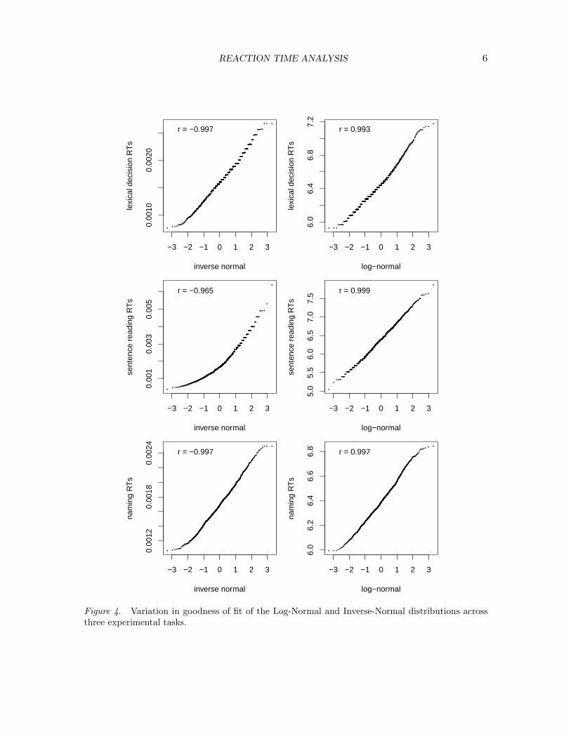
Although Figure 3 might suggest the inverse normal distribution is the optimal choice,the relative goodness of fit of particular theoretical models varies across experimental tasks,however. To illustrate this point, we have randomly chosen one thousand rts from threepriming experiments using visual lexical decision, sentence reading and word naming. Fig-ure 4 indicates that the Inverse Gaussian provides a better fit than the Log-Normal for therts harvested from the lexical decision experiment, just as observed for lexical decision inFigure 3. However, for sentence reading, the Log-Normal outperforms the Inverse Gaussian,while both theoretical models provide equally good fits for the naming data, where even theGamma distribution approaches the same level of goodness of fit (r = 0.995).


470 480 490 500 510 52040

080

012

00

Theoretical Ex−Gaussian

sam

ple

−3 −2 −1 0 1 2 3

0.00

100.

0020

0.00

30

Theoretical Inverse Normal (Wald)

sam

ple

−3 −2 −1 0 1 2 3

6.0

6.5

7.0

Theoretical Log−Normal

sam

ple

400 600 800 100040

080

012

00

Theoretical Gamma

sam

ple

Figure 3. Goodness of fit of four theoretical distributions to response latencies in visual lexicaldecision.

Thus, it is an empirical question which theoretical model provides the best approxi-mation for one’s data. Two considerations are relevant at this stage of the analysis. First, inanalyses aggregating over items to obtain subject means, or aggregating over subjects to ob-tain item means, simulation studies suggest that the Inverse Gaussian may outperform theLog-Normal Ratcliff (1993). Given the abovementioned variability across subjects, items,and tasks, it should be kept in mind that this superiority may be specific to the assump-tions built into the simulations – assumptions that may be more realistic for some subjects,items, and tasks, than for others. The Ex-Gaussian distribution (Luce, 1986) is a theoret-ically interesting alternative, and one might expect it to provide better fits given that ithas one parameter more than Inverse Normal or Log-Normal. Nevertheless, our examplessuggest it is not necessarily one’s best choice – the power provided by this extra parametermay be redundant. Of course, for models with roughly similar goodness of fit, theoreticalconsiderations motivating a given transformation should be given preference.

A second issue is more practical in nature. When rts are transformed, a fitted generallinear model provides coefficients and fitted latencies in another scale than the millisecondtime scale. In many cases, it may be sufficient to report the data on the transformedscale. However, it may be necessary or convenient to visualize partial effects on the originalmillisecond scale, in which case the inverse of the transformation is required. This is noproblem for the Log-Normal and the Inverse-Gaussian transforms, but back-transformingan Ex-Gaussian is far from trivial, as it requires Fourier transformations and division in theFourier domain, or Maximum Entropy deconvolution (see, e.g., Wagenmakers et al., 2008;


−3 −2 −1 0 1 2 3

0.00

100.

0020

inverse normal

lexi

cal d

ecis

ion

RT

sr = −0.997

−3 −2 −1 0 1 2 3

6.0

6.4

6.8

7.2

log−normal

lexi

cal d

ecis

ion

RT

s

r = 0.993

−3 −2 −1 0 1 2 3

0.00

10.

003

0.00

5

inverse normal

sent

ence

rea

ding

RT

s

r = −0.965

−3 −2 −1 0 1 2 3

5.0

5.5

6.0

6.5

7.0

7.5

log−normal

sent

ence

rea

ding

RT

sr = 0.999

−3 −2 −1 0 1 2 3

0.00

120.

0018

0.00

24

inverse normal

nam

ing

RT

s

r = −0.997

−3 −2 −1 0 1 2 3

6.0

6.2

6.4

6.6

6.8

log−normal

nam

ing

RT

s

r = 0.997

Figure 4. Variation in goodness of fit of the Log-Normal and Inverse-Normal distributions acrossthree experimental tasks.


Cornwell & Evans, 1985; Cornwell & Bridle, 1996; Beaudoin, 1999, and references citedthere).

Outliers

Once rts have been properly transformed, the question arises of whether there areatypical and potentially overly influential values that should be removed from the dataset. Strictly speaking, one should differentiate between two types of influential points: theoutliers have acceptable value of the “input” variable while the value of the “response” iseither too large or too small; the extreme values are notably different from the rest of the“input”values. Thus, influential values are those outliers or extreme values which essentiallyalter the estimates, the residuals and/or the fitted values (more about these issues can befound in Hocking, 1996). By defining rt as the measure of behavioural response we impliedthat it may contain outliers and can be affected by extreme values. The question is how todiagnose them and to put them under explicit control.

First of all, physically impossibly short rts (button presses within 5 ms of stimulusonset) and absurdly long latencies (exceeding 5 seconds in a visual lexical decision task withunimpaired undergraduate subjects) should be excluded. After that, more subtle outliersmay still be present in the cleaned data, however. Ratcliff (1993) distinguishes between twokinds of outliers, short versus long response outliers. According to Ratcliff, short outliers“stand alone” while long outliers “hide in the tail” (Ratcliff, 1993, p. 511). Even if longoutliers are two standard deviations above the mean, they may be difficult to locate andisolate. Unfortunately, even a single extreme outlier can considerably increase mean andstandard deviation (Ratcliff, 1979).

There are two complementary strategies for outlier treatment that are worth consid-ering. Before running a statistical analysis, the data can be screened for outliers. However,after a model has been fitted to the data, model criticism may also help identify overlyinfluential outliers. A-priori screening is regular practice in psycholinguistics. By contrast,model criticism seems to be undervalued and underused.

A-priori screening for outliers is a widely accepted practice in traditional by-subjectand by-item analyses. It simply removes all observations that are at a distance of morethan two standard deviations from the mean of the distribution. Nevertheless, there is arisk to this procedure. If the effect “lives” in the right tail of the distribution, as Luce(1986) discussed pointing out that the decision itself may behave as exponential – right-hand component of the distribution, then removing longer and long latencies may in factreduce or cancel out the effect in the statistical analysis (see Ratcliff, 1993). Conversely, ifthe effect is not in the tail, then removing long rts increases statistical power (c.f., Ratcliff,1993; Van Zandt, 2002). For analyses using data aggregated over items or subjects, Ratcliff’sadvice is that cutoffs should be selected as a function of the proportion of responses removed.Up to 15% of the data can be removed, but only if there is no thick right tail, in which caseno more than 5% of the data should be excluded.

We note here that much depends on whether outliers are considered before or aftertransforming the reaction times. Data points that look like outliers before the transforma-tion is applied may turn out to be normal citizens after transformation. More generally, ifthe precondition of normality is well met, then outlier removal before model fitting is notnecessary.


In analyses requiring aggregating over items and/or subjects, the question ariseswhether in the presence of outliers, the mean is the best measure of central tendency.It has been noted that as long as the distribution is roughly symmetrical, the mean willbe an adequate measure of central tendency (c.f., Keppel & Saufley Jr., 1980; Sirkin, 1995;Miller, Daly, Wood, Roper, & Brooks, 1997). For non-symmetrical distributions, however,means might be replaced by medians (see, for example, Whelan, 2008). The median ismuch more insensitive to the skew of the distribution, but at the same time it can be lessinformative. Van Zandt (2002) showed that the median is biased estimator of populationcentral tendency when the population itself is skewed, although this bias is relatively smallfor samples of N ≥ 25. At the same time, the results of Ratcliff (1993)’s simulations showedthat the median of the untransformed rts has much higher variability compared to theharmonic mean H = n/

∑ni=1

1xi

. Unfortunately, the harmonic mean is more sensitive tooutliers and cutoffs then the median. If the noise is equally spread out across experimentalconditions and if an appropriate cutoff is used, then the harmonic mean would be a beterchoice than the median, while the median will be more stable if outliers are not distributedproportionally across conditions.

While a-priori “agressive” screening for outliers is defendable for by-subject and by-item anovas, critically depending on means aggregated over subjects or items, the needfor optimizing central values before data analysis disappears when the analysis targets themore ambitious goal of predicting individual rts using mixed-effects models with subjectsand items as crossed random-effect factors. The mixed-modeling approach allows for milda-priori screening for outliers, in combination with model criticism, a second importantprocedure for dealing with outliers.

In the remainder of this study, we provide various code snippets in the open sourcestatistical programming environment R (http://www.r-project.org/), which provides arich collection of statistical tools. The dataset that we use here for illustrating outlier treat-ment is available in the languageR package as lexdec. Visual lexical decision latencies wereelicited for 21 subjects responding to 79 concrete nouns. Inspection of quantile-quantileplots suggests that a Inverse-Gaussian transformation is optimal. Quantile-quantile plotsfor the individual subjects are brought together in the trellis shown in Figure 5.

> qqmath(~RTinv | Subject, data = lexdec)

The majority of subjects come with distributions that do not depart from normality.However, as indicated by Shapiro tests for normality, there are a few subjects that requirefurther scrutiny, such as subjects A3 and M1.

> f = function(dfr) return(shapiro.test(dfr$RTinv)$p.value)> p = as.vector(by(lexdec, lexdec$Subject, f))> names(p) = levels(lexdec$Subject)> names(p[p < 0.05])

[1] "A3" "M1" "M2" "P" "R1" "S" "V"

Figure 6 presents the densities for the four subjects for which removal of a few extremeoutliers failed to result in normality. The two top leftmost panels (subjects A3 and M1) havelong and thin left tails due to a few outliers, but their removal results in clearly bimodal


quantiles of standard normal

RT

inv

0.00050.00100.00150.00200.00250.0030

−2 0 1 2

A1 A2

−2 0 1 2

A3 C

−2 0 1 2

D

I J K M1

0.00050.00100.00150.00200.00250.0030

M20.00050.00100.00150.00200.00250.0030

P R1 R2 R3 S

T1 T2 V W1

0.00050.00100.00150.00200.00250.0030

W20.00050.00100.00150.00200.00250.0030

Z

Figure 5. By-subject quantile-quantile plots for the inverse-transformed reaction times (visuallexical-decision).

distributions, as can be seen in the corresponding lower panels. The density for subject M2shows a leftward skew without outliers, but after removing some highest and lowest valuesdistribution gets two modes of almost equal hight. Conversely, the density for subject V isagain bimodal before, and gently skewed to the left after the removal.

Minimal trimming for subjects A3, M1, P, R1, S resulted in a new data frame (thedata structure in R for tabular data), which we labeled lexdec2. With the trimming welost 2.7% of the original data, or 45 data points. For comparison, we also created a dataframe with all data points removed that exceeded 2 standard deviations from either subjector item means (lexdec3). This data frame comes with a loss of 134 datapoints (8.1% ofthe data). These data frames allow us to compare models with different outlier-handlingstrategies. (In what follows, we multiplied the inversely transformed rts by −1000 so thatcoefficients will have the same sign as for models fitted to the untransformed latencies, at thesame time avoiding very small values and too restricted range for the dependent variable.)

A model fitted to all data, without any outlier removal:

> lexdec.lmer = lmer(-1000 * RTinv ~ NativeLanguage + Class + Frequency ++ Length + (1 | Subject) + (1 | Word), data = lexdec)


0.0010 0.0020

050

015

00

inverse RT

Den

sity

A3

0.0005 0.0015 0.0025

050

010

0015

00

inverse RT

Den

sity

M1

0.0005 0.0020

020

060

010

00

inverse RT

Den

sity

M2

0.0010 0.0020

050

010

0015

00

inverse RT

Den

sity

V

0.0014 0.0018

050

015

0025

00

inverse RT

Den

sity

A3

0.0014 0.0020 0.0026

050

010

0020

00

inverse RT

Den

sity

M1

0.0014 0.0020

050

015

00

inverse RT

Den

sity

M2

0.0010 0.0016

050

015

00

inverse RT

Den

sity

V

Figure 6. Density plots for subjects for which the Inverse-Gaussian transform does not resultin normality (visual lexical-decision). Upper panels represent untrimmed data, while lower panelsdepict the distributions for two subjects after minimal trimming.

> cor(fitted(lexdec.lmer), -1000 * lexdec$RTinv)^2[1] 0.5171855

performs less well in terms of R2 than a model with the traditional aggressive a-priori datascreening:

> lexdec.lmer3 = lmer(-1000 * RTinv ~ NativeLanguage + Class ++ Frequency + Length + (1 | Subject) + (1 | Word), data = lexdec3)> cor(fitted(lexdec.lmer3), -1000 * lexdec3$RTinv)^2[1] 0.59104

while mild initial data screening results in a model with an intermediate R2:

> lexdec2.lmer = lmer(-1000 * RTinv ~ NativeLanguage + Class ++ Frequency + Length + (1 | Subject) + (1 | Word), data = lexdec2)

> cor(fitted(lexdec2.lmer), -1000 * lexdec2$RTinv)^2[1] 0.5386757

Inspection of the residuals of this model (lexdec2.lmer) shows that it is stressed,and fails to adequately model longer response latencies, as can be seen in the lower leftpanel of Figure 7. To alleviate the stress from the model, we remove data points withabsolute standardized residuals exceeding 2.5 standard deviations:

> lexdec2A = lexdec2[abs(scale(resid(lexdec2.lmer))) < 2.5, ]> lexdec2A.lmer = lmer(-1000 * RTinv ~ NativeLanguage + Class ++ Frequency + Length + (1 | Subject) + (1 | Word), data = lexdec2A)> cor(fitted(lexdec2A.lmer), -1000 * lexdec2A$RTinv)^2


−3 −1 0 1 2 3

−1.

00.

01.

0

Theoretical Quantiles

Sam

ple

Qua

ntile

s

full data

−3 −1 0 1 2 3

−0.

50.

00.

5


Sam

ple

Qua

ntile

s

agressive a−priori trimming

−3 −1 0 1 2 3

−1.

00.

00.

51.

0


Sam

ple

Qua

ntile

s

minimal a−priori trimming, no model criticism

−3 −1 0 1 2 3

−0.

6−

0.2

0.2

0.6


Sam

ple

Qua

ntile

s

minimal trimming and model criticism

Figure 7. Quantile-quantile plots for the models with different strategies of outlier removal.

[1] 0.5999562

The last model, which combines both mild initial data screening and model criticism,outperforms all other models in terms of R2. Compared to the traditional aggressive datatrimming procedure, it succeeds in doing so by achieving reasonable closeness to normal-ity, while removing fewer data points (82 versus 134). The quantile-quantile plot for theresiduals of this model is shown in the lower right panel of Figure 7.

What this example shows is that a very good model can be obtained with minimala-priori screening, combined with careful post-fitting model criticism based on evidencethat the residuals of the fitted model do not follow a normal distribution. If there is noevidence for stress in the model fit, then removal of outliers is not necessary and should notbe carried out. Furthermore, there are many diagnostics for identifying overly influentialoutliers, such as variance inflation factors and Cook’s distance, which may lead to a moreparsimoneous removal of data points compared to the procedure illustrated in the presentpaper. It simply errs on the conservative side, but allows the researcher to quickly assesswhether or not an effect is carried by the majority of data points.

We note here that it may well be that the data points removed due to model criti-cism reflect decision processes distinct from the processes subserving lexical retrieval, whichtherefore may require further scrutiny when these decision processes are targeted by the


Lag

Acf

−0.20.20.61.0

0 510 20

s1 s2

0 510 20

s3 s4

0 510 20

s5 s6

0 510 20

s7

s8 s9 s10 s11 s12 s13

−0.20.20.61.0

s14−0.2

0.20.61.0

s15 s16 s17 s18 s19 s20 s21

s22 s23 s24 s25 s26 s27

−0.20.20.61.0

s28−0.2

0.20.61.0

s29 s30 s31 s32 s33 s34 s35

s36

0 510 20

s37 s38

0 510 20

s39

−0.20.20.61.0

s40

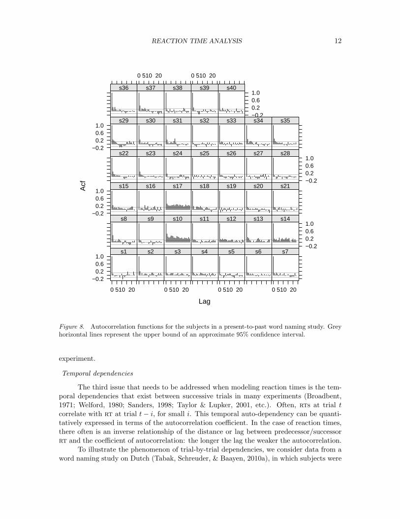
Figure 8. Autocorrelation functions for the subjects in a present-to-past word naming study. Greyhorizontal lines represent the upper bound of an approximate 95% confidence interval.

experiment.

Temporal dependencies

The third issue that needs to be addressed when modeling reaction times is the tem-poral dependencies that exist between successive trials in many experiments (Broadbent,1971; Welford, 1980; Sanders, 1998; Taylor & Lupker, 2001, etc.). Often, rts at trial tcorrelate with rt at trial t− i, for small i. This temporal auto-dependency can be quanti-tatively expressed in terms of the autocorrelation coefficient. In the case of reaction times,there often is an inverse relationship of the distance or lag between predecessor/successorrt and the coefficient of autocorrelation: the longer the lag the weaker the autocorrelation.

To illustrate the phenomenon of trial-by-trial dependencies, we consider data from aword naming study on Dutch (Tabak, Schreuder, & Baayen, 2010a), in which subjects were


shown a verb in the present (or paste) tense and were requested to name the correspondingpast (or present) tense form. Figure 8 shows the autocorrelation functions for the timeseries of rts for each of the subjects, obtained by applying acf.fnc function from thelanguageR package (version 1.0), which builds on the acf function from stats package inR and lattice graphics.

> acf.fnc(dat, group = "Subj", time = "Trial", x = "RT", plot = TRUE)

Many subjects show significant autocorrelations at short lags, notably at a lag of one.For some subjects, such as s10 and s17, significant autocorrelations are found across amuch wider span of lags. As the generalized linear model (and special cases such as analysisof variance) build on the assumption of the independence of observations, correctivemeasures are required. In what follows, we illustrate how this temporal correlation can beremoved by taking as example results from subject s10. A regression model is fitted tothis subject’s responses, with a log-transform for the naming latencies, using a quadratic(non-orthogonal) polynomial for word frequency, and with two covariates to bring temporaldependencies under control: Trial and the Preceding RT. The coefficients of the fittedmodel are listed in Table 1.

> exam.ols = ols(RT ~ pol(Frequency, 2) + rcs(Trial) + PrecedingRT,+ data = exam)

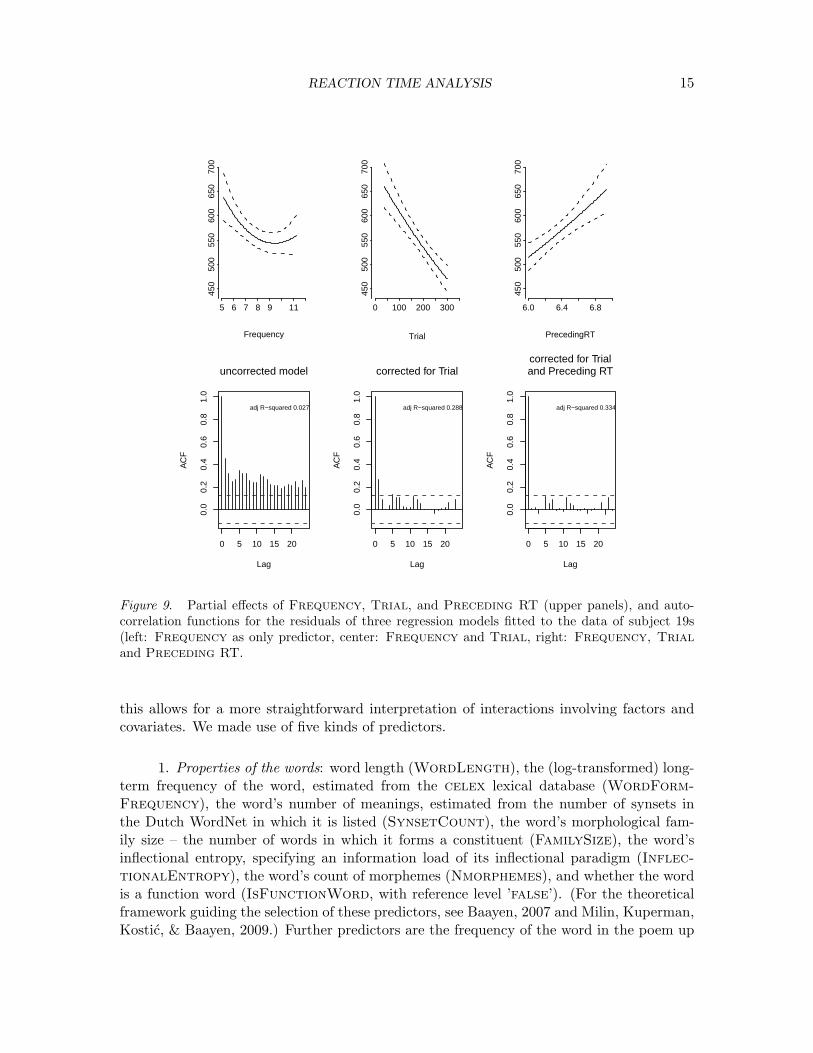
The first temporal control, Trial, represents rank-order of a trial in its exper-imental sequence. Since trials are usually presented to each participant in different,(pseudo)randomized sequence, rank-ordering is unique between participants. In general,this control covariate models the large-scale flow of the experiment, representing learning(latencies becoming shorter) or fatigue (latencies becoming longer as the experiment pro-ceeds). For the present subject (s10), responses were executed faster as the experimentproceeded, suggesting adaptation to the task (upper left panel of Figure 9). It is worthnoting that the trial number in an experimental session may enter into an interaction withone or more critical predictors, as in the eye-tracking study of Bertram, Kuperman, andBaayen (2010). Figure 9 indicates that the present learning effect is greater in magnitudethan the effect of frequency.

The second temporal control covariate is the latency at the preceding trial (Preced-ing RT). For the initial trial, this latency is imputed from the other latencies in the timeseries (often as mean reaction time). The current latency and the preceding latency arehighly correlated (r = 0.46, t(250) = 8.13, p � 0.0001). The effect size of Preceding RTis substantial, and greater than the effect size of Frequency (see Figure 9). Studies inwhich this predictor has been found to be significant range from speech production (picturenaming, Tabak, Schreuder, & Baayen, 2010b), and speech comprehension (auditory lexi-cal decision, Baayen, Wurm, & Aycock, 2007; Balling & Baayen, 2008), to reading (visuallexical decision, De Vaan, Schreuder, & Baayen, 2007; Kuperman, Schreuder, Bertram, &Baayen, 2009; and progressive demasking, Lemhoefer et al., 2008).

A model with just Frequency as predictor has an R-squared of 0.027. By addingTrial as predictor, the R-squared improves to 0.288. Including both Trial and Pre-ceding RT results in an R-squared of 0.334. The lower panels of Figure 9 illustrate that


Value Std. Error t pIntercept 5.6850 0.4730 12.0179 0.0000Frequency (linear) -0.1657 0.0610 -2.7179 0.0070Frequency (quadratic) 0.0088 0.0036 2.4282 0.0159Trial -0.0013 0.0002 -6.3415 0.0000Preceding RT 0.2570 0.0601 4.2777 0.0000

Table 1: Coefficients of an ordinary least-squares regression model fitted to the naming latencies ofsubject 19s.

including Trial as predictor removes most of the autocorrelation at later lags, but a sig-nificant autocorrelation persists at lag 1. By including Preceding RT as predictor, thisautocorrelation is also removed.

Across many experiments, we have found that including variables such as Trial andPreceeding RT in the model not only avoids violating the assumptions of linear modeling,but also helps improving the fit and clarifying the role of the predictors of interest (see, e.g.,De Vaan et al., 2007).

An example of mixed-effects modeling

Mixed-effects models offer the researcher the possibility of analyzing data with morethan one random-effect factor – a factor with levels sampled from some large population.In psycholinguistics, typical random-effect factors are subjects (usually sampled from theundergraduate students that happen to be enrolled at one’s university) and items (e.g.,syllables, words, sentences). Before the advent of mixed-models, data with repeated mea-surements for both subjects and items had to be analyzed by aggregating over items toobtain subject means, aggregating over subjects to obtain item means, or both (see,e.g.,Clark, 1973; Forster & Dickinson, 1976; Raaijmakers, Schrijnemakers, & Gremmen, 1999,and references cited there). mixed-models obviate the necessity of prior averaging, andthereby offer the researcher the far more ambitious goal to model the individual response ofa given subject to a given item. Importantly, mixed-models offer the possibility of bringingsequential dependencies, as described in the preceding section, into the model specification.They also may offer a small increase in power, and better protection against Type II errors.In what follows, we discuss, a large dataset illustrating some of the novel possibilities offeredby the mixed-modeling framework building on prior introductions (here we build on priorintroductions given by Pinheiro & Bates, 2000; Baayen et al., 2008; Jaeger, 2008; Quene &Bergh, 2008, etc.). Analyses are run with the lme4 package for R (Bates & Maechler, 2009).

The data

The dataset comprises 275996 self-paced reading latencies elicited through a webinterface from 326 subjects reading 2315 words distributed over 87 poems in the anthologyof Breukers (2006). Subjects included students in an introductory methods class, as wellas their friends and relatives. For fixed-effect factors, we made use of contrast coding, as


Frequency

5 6 7 8 9 11

450

500

550

600

650

700

Trial

0 100 200 300

450

500

550

600

650

700

PrecedingRT

6.0 6.4 6.8

450

500

550

600

650

700

0 5 10 15 20

0.0

0.2

0.4

0.6

0.8

1.0

Lag

AC

F

uncorrected model

adj R−squared 0.027

0 5 10 15 20

0.0

0.2

0.4

0.6

0.8

1.0

Lag

AC

F

corrected for Trial


0 5 10 15 20

0.0

0.2

0.4

0.6

0.8

1.0

Lag

AC

F

corrected for Trialand Preceding RT


Figure 9. Partial effects of Frequency, Trial, and Preceding RT (upper panels), and auto-correlation functions for the residuals of three regression models fitted to the data of subject 19s(left: Frequency as only predictor, center: Frequency and Trial, right: Frequency, Trialand Preceding RT.

this allows for a more straightforward interpretation of interactions involving factors andcovariates. We made use of five kinds of predictors.

1. Properties of the words: word length (WordLength), the (log-transformed) long-term frequency of the word, estimated from the celex lexical database (WordForm-Frequency), the word’s number of meanings, estimated from the number of synsets inthe Dutch WordNet in which it is listed (SynsetCount), the word’s morphological fam-ily size – the number of words in which it forms a constituent (FamilySize), the word’sinflectional entropy, specifying an information load of its inflectional paradigm (Inflec-tionalEntropy), the word’s count of morphemes (Nmorphemes), and whether the wordis a function word (IsFunctionWord, with reference level ’false’). (For the theoreticalframework guiding the selection of these predictors, see Baayen, 2007 and Milin, Kuperman,Kostic, & Baayen, 2009.) Further predictors are the frequency of the word in the poem up


to the point of reading (LocalFrequency), the frequency of the rhyme in the poem up tothe point of reading (LocalRhymeFreq), and the frequency of the word’s onset up to thepoint of reading (LocalOnsetFreq). Rhymes and onsets were calculated for the last andfirst syllables of the word, respectively. Onsets were defined as all consonants preceding thevowel of the syllable, and rhymes were defined as the vowel and all tautosyllabic followingconsonants. Note that these last three predictors are not available to analyses that cruciallyrequire aggregation over subjects and/or items.Unsurprisingly, LocalRhymeFreq and LocalOnsetFreq enter into strong correlationswith LocalFrequency (r > 0.6). We therefore decorrelated LocalRhymeFreq fromLocalFrequency by regressing LocalRhymeFreq on LocalFrequency and takingthe residuals as new, orthogonalized, predictor. The same procedure was followed forLocalOnsetFreq. The two residualized variables correlated well with the original mea-sures (r = 0.77 for LocalRhymeFreq and r = 0.80 for LocalOnsetFreq). Thus,decorrelation was justified to control for the collinearity, but, moreover, it did not changethe nature of the original predictors.

2. Properties of the lines of verse: the length of the sentence (SentenceLength),the position of the word in the sentence (Position, a fixed-effect factor with levels ’Initial’,’Mid’, ’Final’, with ’Initial’ as reference level), whether the word was followed by a punc-tiation mark (PunctuationMark, reference level ’false’), and the number of words thereader is into the line (NumberOfWordsIntoLine).

3. Properties of the subject: Age (ranging from 13 to 63, median 23), Sex (187women, 142 men), Handedness (39 left handed, 290 right handed), and two variableselicited during a questionairre at the end of the experiment. This questionaire asked subjectsto indicate (through a four-way multiple choice) how many poems they estimated readingon a yearly basis, this estimate was log-transformed (PoemsReadYearly). The timerequired to reach this choice was also recorded, and log-transformed (ChoiceRT).

4. Longitudinal predictors: Trial, the number of words read at the point of reading(ranging from 1 to 1270), and Preceding RT, the self-paced reading latency at the pre-ceding word. These two predictors are not available for analyses based on aggregated dataas well.

5. Three random-effect factors: Subject, Word, and Poem. Note that we caninclude more than two random-effect factors if there are multiple kinds of repeated measuresin the dat; no separate F1, F2 F3, . . . , Fn tests need to be carried out.

A model

A stepwise variable selection procedure resulted in a model that is specified asfollows, using the lmer function from lme4 package in R:

poems.lmer = lmer(RT ~

WordLength + I(WordLength^2) +WordFormFrequency + I(WordFormFrequency^2)+SynsetCount + FamilySize + InflectionalEntropy +IsFunctionWord + Nmorphemes +


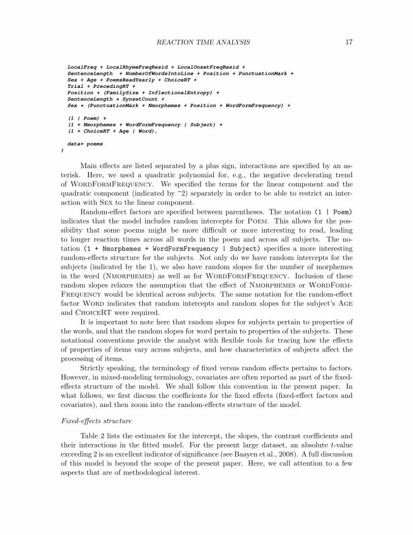
LocalFreq + LocalRhymeFreqResid + LocalOnsetFreqResid +SentenceLength + NumberOfWordsIntoLine + Position + PunctuationMark +Sex + Age + PoemsReadYearly + ChoiceRT +Trial + PrecedingRT +Position * (FamilySize + InflectionalEntropy) +SentenceLength * SynsetCount +Sex * (PunctuationMark + Nmorphemes + Position + WordFormFrequency) +

(1 | Poem) +(1 + Nmorphemes + WordFormFrequency | Subject) +(1 + ChoiceRT + Age | Word),

data= poems)

Main effects are listed separated by a plus sign, interactions are specified by an as-terisk. Here, we used a quadratic polynomial for, e.g., the negative decelerating trendof WordFormFrequency. We specified the terms for the linear component and thequadratic component (indicated by ^2) separately in order to be able to restrict an inter-action with Sex to the linear component.

Random-effect factors are specified between parentheses. The notation (1 | Poem)indicates that the model includes random intercepts for Poem. This allows for the pos-sibility that some poems might be more difficult or more interesting to read, leadingto longer reaction times across all words in the poem and across all subjects. The no-tation (1 + Nmorphemes + WordFormFrequency | Subject) specifies a more interestingrandom-effects structure for the subjects. Not only do we have random intercepts for thesubjects (indicated by the 1), we also have random slopes for the number of morphemesin the word (Nmorphemes) as well as for WordFormFrequency. Inclusion of theserandom slopes relaxes the assumption that the effect of Nmorphemes or WordForm-Frequency would be identical across subjects. The same notation for the random-effectfactor Word indicates that random intercepts and random slopes for the subject’s Ageand ChoiceRT were required.

It is important to note here that random slopes for subjects pertain to properties ofthe words, and that the random slopes for word pertain to properties of the subjects. Thesenotational conventions provide the analyst with flexible tools for tracing how the effectsof properties of items vary across subjects, and how characteristics of subjects affect theprocessing of items.

Strictly speaking, the terminology of fixed versus random effects pertains to factors.However, in mixed-modeling terminology, covariates are often reported as part of the fixed-effects structure of the model. We shall follow this convention in the present paper. Inwhat follows, we first discuss the coefficients for the fixed effects (fixed-effect factors andcovariates), and then zoom into the random-effects structure of the model.

Fixed-effects structure

Table 2 lists the estimates for the intercept, the slopes, the contrast coefficients andtheir interactions in the fitted model. For the present large dataset, an absolute t-valueexceeding 2 is an excellent indicator of significance (see Baayen et al., 2008). A full discussionof this model is beyond the scope of the present paper. Here, we call attention to a fewaspects that are of methodological interest.


Estimate Std. Error t valueIntercept 3.7877 0.0244 155.2758WordLength -0.0024 0.0031 -0.7789I(WordLength^2) 0.0010 0.0002 4.7543WordFormFrequency -0.0240 0.0058 -4.0971I(WordFormFrequency^2) 0.0051 0.0018 2.8385SynsetCount 0.0240 0.0045 5.3294FamilySize -0.0042 0.0013 -3.1877InflectionalEntropy -0.0122 0.0027 -4.4556IsFunctionWordTRUE 0.0055 0.0061 0.8920Nmorphemes 0.0005 0.0013 0.3923LocalFreq -0.0048 0.0004 -11.7279LocalRhymeFreqResid 0.0029 0.0008 3.7343LocalOnsetFreqResid -0.0062 0.0007 -8.5043SentenceLength -0.0016 0.0005 -2.8406NumberOfWordsIntoLine 0.0029 0.0004 7.6266Position = Final 0.0608 0.0061 9.8940Position = Mid -0.0621 0.0038 -16.2994PunctuationMark = TRUE 0.1496 0.0031 48.8943Sex = Male -0.0516 0.0149 -3.4612Age 0.0034 0.0005 6.2285PoemsReadYearly -0.0111 0.0060 -1.8456ChoiceRT 0.0543 0.0087 6.2233Trial -0.0002 0.0000 -73.1891PrecedingRT 0.3957 0.0017 234.5453FamilySize : Position = Final 0.0028 0.0013 2.2295FamilySize : Position = Mid 0.0035 0.0008 4.4843InflectionalEntropy : Position = Final 0.0140 0.0027 5.1897InflectionalEntropy : Position = Mid 0.0077 0.0021 3.7411SynsetCount : SentenceLength -0.0023 0.0004 -5.7932PunctuationMark = TRUE : Sex = Male -0.0291 0.0040 -7.3039Nmorphemes : Sex = Male -0.0024 0.0013 -1.9004Position = Final : Sex = Male -0.0144 0.0044 -3.2749Position = Mid : Sex = Male -0.0121 0.0031 -3.8598WordFormFrequency : Sex = Male 0.0110 0.0045 2.4410

Table 2: Estimated coefficients, standard errors, and t-values for the mixed-model fitted to theself-paced reading latencies elicited for Dutch poems.


First, it is noteworthy that the two coefficients with the largest absolute t-valuesare two control predictors that handle temporal dependencies: Trial and PrecedingRT.Their presence in the model not only helps satisfy to a better extent the independenceassumption of the linear model, but also contribute to a more precise model with a smallerresidual error. Simply stated, these predictors allow a more precise estimation of the con-tributions of the other, theoretically more interesting, predictors.

Second, our model disentangles the contributions of long-term frequency (as gaugedby frequency of occurrence in a corpus) from the contribution of the frequency with whichthe word has been used in the poem up to the point of reading. Long-term frequency(WordFormFrequency) emerged with a negative decelerating function, with diminishingfacilitation for increasing frequencies. Short-term frequency (LocalFreq) made a smallbut highly significant independent contribution. We find it remarkable that this short-term(i.e., episodic) frequency effect is detectable in spite of massive experimental noise.

Independently of short-term frequency, the frequency of the rhyme (Local-RhymeFreqResid) and the frequency of the onset (LocalOnsetFreqResid) reachedsignificance, with the local frequency of the rhyme emerging as inhibitory, and the localfrequency of the onset as facilitatory. Thus two classic poetic devices, end-rhyme and al-literation, emerge with opposite sign. The facilitation for alliteration may arise due tocohort-like preactivation of words sharing word onset, the inhibition for rhyming may re-flect an inhibitory neighborhood density effect, or a higher cognitive effect such as attentionto rhyme when reading poetry. Crucially, the present experiment shows that in the mixed-modeling framework effects of lexical similarity can be studied not only in the artificialcontext of controlled factorial experiments, but also in the natural context of the reading ofpoetry.

Third, the present model provides some evidence for sexual differentiation in lexicalprocessing. Ullman and colleagues (Ullman et al., 2002; Ullman, 2007) have argued thatfemales have an advantage in declarative memory, while males might have an advantagein procedural memory. With respect to the superior verbal memory of females (see alsoKimura, 2000), note that the negative decelerating effect of long-term frequency (Word-FormFrequency) is more facilitatory for females than for males: for males, the linearslope of WordFormFrequency equals −0.0240 + 0.0110 = −0.0130 while for females itis −0.0240. In other words, the facilitation from word frequency is almost twice as large forfemales compared to males.

There is also some support for an interaction of the morphological complexity (Nmor-phemes) by Sex. While for females, Nmorphemes has zero slope (β = 0.0005, t = 0.39),males show slightly shorter reading times as the number of morphemes increases (β =0.0005− 0.0024 = −0.0019, t = −1.90, p < 0.05, one-tailed test). This can be construed asevidence for a greater dependence on procedural memory for males. The evidence, however,is weaker than the evidence for the greater involvement of declarative memory for females.We will return to these interactions in more detail below.

Random-effects structure

The random-effects structure of our model is summarized in Table 3. There are threerandom-effect factors, labeled as ‘Groups’: Word, Subject, and Poem. For each, the tablelists the standard deviation for the adjustments to the intercepts. For Word and Subject,


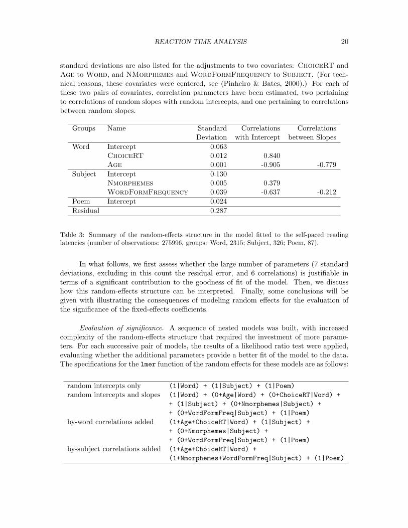
standard deviations are also listed for the adjustments to two covariates: ChoiceRT andAge to Word, and NMorphemes and WordFormFrequency to Subject. (For tech-nical reasons, these covariates were centered, see (Pinheiro & Bates, 2000).) For each ofthese two pairs of covariates, correlation parameters have been estimated, two pertainingto correlations of random slopes with random intercepts, and one pertaining to correlationsbetween random slopes.

Groups Name Standard Correlations CorrelationsDeviation with Intercept between Slopes

Word Intercept 0.063ChoiceRT 0.012 0.840Age 0.001 -0.905 -0.779

Subject Intercept 0.130Nmorphemes 0.005 0.379WordFormFrequency 0.039 -0.637 -0.212

Poem Intercept 0.024Residual 0.287

Table 3: Summary of the random-effects structure in the model fitted to the self-paced readinglatencies (number of observations: 275996, groups: Word, 2315; Subject, 326; Poem, 87).

In what follows, we first assess whether the large number of parameters (7 standarddeviations, excluding in this count the residual error, and 6 correlations) is justifiable interms of a significant contribution to the goodness of fit of the model. Then, we discusshow this random-effects structure can be interpreted. Finally, some conclusions will begiven with illustrating the consequences of modeling random effects for the evaluation ofthe significance of the fixed-effects coefficients.

Evaluation of significance. A sequence of nested models was built, with increasedcomplexity of the random-effects structure that required the investment of more parame-ters. For each successive pair of models, the results of a likelihood ratio test were applied,evaluating whether the additional parameters provide a better fit of the model to the data.The specifications for the lmer function of the random effects for these models are as follows:

random intercepts only (1|Word) + (1|Subject) + (1|Poem)random intercepts and slopes (1|Word) + (0+Age|Word) + (0+ChoiceRT|Word) +

+ (1|Subject) + (0+Nmorphemes|Subject) ++ (0+WordFormFreq|Subject) + (1|Poem)

by-word correlations added (1+Age+ChoiceRT|Word) + (1|Subject) ++ (0+Nmorphemes|Subject) ++ (0+WordFormFreq|Subject) + (1|Poem)

by-subject correlations added (1+Age+ChoiceRT|Word) +(1+Nmorphemes+WordFormFreq|Subject) + (1|Poem)


The first model has random intercepts only, the second has both random interceptsand random slopes, but no correlation parameters. The third model adds in the by-wordcorrelation parameters. The fourth model is our final model, with the full random-effectsstructure in place. In particular, the notation (1+WordFormFreq|Subject) instructs the al-gorithm to estimate a correlation parameter for the by-subject random intercepts and the by-subject random slopes for WordFormFrequency. Conversely, the notation (1|Subject)+ (0+WordFormFreq|Subject) specifies that the by-subject random intercepts should beestimated as independent of the by-subject random slopes for WordFormFrequency,i.e., without investing a parameter for their correlation.

Table 4 summarizes the results of the likelihood ratio tests for the sequence of nestedmodels (including also log-likelihood, aic and bic values). The test statistic follows achi-squared distribution, with the difference in the number of parameters between the morespecific and the more general model as the degrees of freedom. The chi-squared test statisticis twice the ratio of the two log-likelihoods. As we invest more parameters in the random-effects structure (see the column labeled ‘df’, which lists the total number of parameters,including the 34 fixed-effects coefficients), goodness of fit improves, as witnessed by decreas-ing values of aic and bic, and increasing values of the log likelihood. For each pairwisecomparison, the increase in goodness of fit is highly significant. Other random slopes werealso considered, but were not supported by likelihood ratio tests.

df aic bic log-likelihood χ2 dfχ2 prandom intercepts only 38 104893 105293 -52408random intercepts and slopes 42 101103 101545 -50509 3797.9 4 � 0.0001by-word correlations added 45 101029 101503 -50470 79.4 3 � 0.0001by-subject correlations added 48 100880 101386 -50392 155.2 3 � 0.0001

Table 4: Likelihood ratio tests comparing models with increasingly complex random-effects structure:a model with random intercepts only, a model with by-subject and by-word random intercepts andslopes, but no correlation parameters, a model adding in the by-word correlation parameters, andthe full model with also by-subject correlation parameters. (df: the number of parameters in themodel, including the coefficients of the fixed-effect part of the model.)

Interpretation of the random effects structure. Given that the present complexrandom-effects structure is justified, the question arises how to interpret the parameters.Scatterplot matrices, as shown in Figure 10, often prove to be helpful guides. The leftmatrix visualizes the random effects structure for words, the right matrix that for sub-jects, where in the left matrix each dot represents a word, and in the right matrix a dotrepresents a subject. For each pair of covariates, the blups (the best linear unbiased pre-dictors) for the words (left) and subjects (right) are shown. The blups can be understoodas the adjustments required to the population estimates of intercept and slopes to make themodel precise for a given word or subject. Correlational structure is visible in all panels, asexpected given the 6 correlation parameters in the model specification.

First consider the left matrix in Figure 10. It shows much tighter correlations, whicharise because in this experiment words were partially nested under poem and subject. Withlimited information on the variability across subjects and in respect to words’ processing


(Intercept)

−0.02 0.02

−0.

20.

00.

2

−0.

020.

02

ChoiceRT

−0.2 0.0 0.2 −0.003 0.000−

0.00

30.

000

Age

(Intercept)

−0.005 0.005

−0.

30.

00.

3

−0.

005

0.00

5

Nmorphemes

−0.3 0.0 0.3 −0.15 0.00

−0.

150.

00

WordFormFrequency

Figure 10. Visualization of the correlation structure of the random intercepts and slopes for Word(left) and Subject (right) by means of scatterplot matrices.

difficulty, estimated correlations are tight. In the first row of the left panel, differences in theintercept (on the vertical axis) represent differences in the baseline difficulty of words. Easywords (with short self-paced reading latencies) have downward adjustments to the intercept,difficult words (with long latencies) have upward adjustments. These adjustments for theintercept correlate positively with the adjustments for the slope of the ChoiceRT, the timerequired for a subject to complete the final multiple choice question about the number ofpoems read on a yearly basis. The estimated population coefficient for this predictor isβ = 0.0543 (c.f., Table 2): Careful, slow respondents are also slow and careful readers.Across words, the adjustments to this population slope for Choice RT give rise to word-specific slopes ranging from 0.022 to 0.109. The positive correlation of the by-word interceptsand these by-word slopes indicates that for difficult words (large positive adjustments tothe intercept), the difference between the slow and fast responders to the multiple choicequestion is more pronounced (as reflected by upward adjustments resulting in even steeperpositive slopes). Conversely, for words with the larger downward adjustments to the slopeof ChoiceRT, the easy words, the difference between the slow (presumably careful andprecise) and fast (more superficial) responders is attenuated.

Next, from the fixed-effects part of the model, we know that older subjects are char-acterized by longer reaction times (β = 0.0034). The effect of Age is not constant acrosswords, however. For some words (with maximal downward adjustment for Age), the effectof Age is actually cancelled out, while there are also words (with positive adjustments) forwhich the effect of Age is felt even more strongly. The negative correlation for the by-wordadjustments to the slope for Age and the by-word adjustments to the intercept indicatesthat it is for the more difficult words that the effect of Age disappears, and that it is forthe easier words that the effect of Age manifests itself most strongly.

The negative correlation for Age and Choice RT indicates that the words for which


greater Age leads to the longest responses are also the words for which elongated choicebehavior has the smallest processing cost. The three correlations considered jointly indicatethat the difficult words (large positive adjustments to the intercept) are the words wherecareful choice behavior is involved, but not so much Age, whereas the easy words (downwardadjusted intercepts) are those where differences in age are most clearly visible, but not choicebehavior.

The scatterplot matrix in the right panel of Figure 10 visualizes the less tight corre-lational structure for the by-subject adjustments to intercept and slopes. The adjustmentsto the intercept position subjects with respect to the average response time. Subjects withlarge positive blups for the intercept are slow subjects, those with large negative blups arefast responders.

The population slope for the count of morphemes in the word (Nmorphemes) is 0for females and -0.002 for males. By-subject adjustments range from -0.008 to +0.008,indicating substantial variability exceeding the group difference. Subjects with a morenegative slope for Nmorphemes tend to be faster subjects, those with a positive slope tendto be the slower subjects.

The linear coefficient of WordFormFrequency estimated for the population is−0.024 for females and −0.013 for males. For different female subjects, addition of theadjustments results in slopes ranging from −0.178 to 0.051, for males, this range is shiftedupwards by 0.011. For most subjects, we have facilitation, but for a few subjects there is noeffect or perhaps even an “anti-frequency” effect. The negative correlation for the by-subjectadjustments to the intercept and to the slope of frequency indicates that faster subjects,with downward adjustments for the intercept, are characterized by upward adjustment forWordFormFrequency slopes. Hence, these fast subjects have reduced facilitation oreven inhibition from WordFormFrequency. Conversely, slower subjects emerge withstronger facilitation.

Interestingly, the correlation of the adjustments for WordFormFrequency andNmorphemes is negative, indicating that subjects who receive less facilitation from fre-quency obtain more facilitation from morphological complexity and vice versa.

Consequences for the fixed-effects coefficients. Careful modeling of the correlationalstructure of the random effects is important not only for tracing cognitive trade-offs suchas observed for storing (WordFormFrequency) and parsing (Nmorphemes), it is alsocrucial for the proper evaluation of interactions with fixed-effect factors partitioning sub-jects or items into subsets. Consider the interaction of Sex by WordFormFrequencyand Sex by Nmorphemes. In the full model, the former interaction receives good sup-port with t = 2.44, while the latter interaction fails to reach significance (t = −1.90).However, in models having only random intercepts for subjects, t-values increase to 7.73and −1.99 respectively. These models are not conservative enough, however. They over-value the interactions in the fixed-effects part of the model, while falling short with respectto their goodness of fit, which could have been improved substantially by allowing intothe model individual differences between subjects with respect to WordFormFrequencyand Nmorphemes. In other words, when testing for interactions involving a group variablesuch as Sex, the interaction should survive inclusion of random slopes, when such randomslopes are justified by likelihood ratio tests. In the present example, the interaction of


Sex by WordFormFrequency survives inclusion of random slopes for WordFormFre-quency, but the interaction with Nmorphemes does not receive significant support.

Model Criticism

To complete the analysis, we need to examine our model critically with respect topotential distortions due to outliers. Before modeling, the data were screened for artificialresponses (such as those generated by subjects holding the spacebar down to skip poemsthey did not like), but no outliers were removed. As the presence of outliers may causestress in the model, we removed datapoints with absolute standardized residuals exceeding2.5 standard deviations (2.7% of the data). The trimmed model was characterized byresiduals that approximated normality more closely, as expected.

Model criticism can result in three different outcomes for a given coefficient. A coef-ficient that was significant may no longer be so after trimming. If we recall the differencebetween the outliers and the extreme values, in this case it is likely that a few extreme valuesare responsible for the effect. Given that the vast majority of data points do not supportthe effect, we then conclude that there is no effect. Conversely, a coefficient that did notreach significance may be significant after model criticism. In that case, a small number ofoutliers was probably masking an effect that is actually supported by the majority of datapoints. In this case we conclude there is a significant effect. Data trimming may also notaffect the significance of a predictor in case the influential values have little leverage withrespect to that particular predictor.

For the present data, model criticism did lead to a revision of the coefficients forthe interactions of Sex by Nmorphemes and Sex by WordFormFrequency. For both,evidence for a significant interaction increased. The t-value for the coefficient of the inter-action of Sex by WordFormFrequency increased from 2.44 to 2.71, and the coefficientfor Sex by Nmorphemes showed absolute increase from −1.90 to −2.77. We note thattrimming does not automatically result in increased evidence for significance. For instance,the support for the predictor PoemsReadYearly decreased after trimming, as indicatedby the t-value, with decreased absolute values from −1.85 to −1.75.

In the light of these considerations, we conclude that this data set provides evidencesupporting the hypothesis of Ullman and colleagues that the superior declarative memory ofwomen affords stronger facilitation from word frequency, whereas males show faster process-ing of morphologically complex words, possibly due to a greater dependence on proceduralmemory. Although these differences emerge as significant, over and above the individualdifferences that are also significant, they should be interpreted with caution, as the effectsizes are small. The facilitation from WordFormFrequency, evaluated by comparing theeffects for the minimum and maximum word frequencies, was 67 ms for females and 40 msfor males; an advantage of 27 ms for females. The advantage in morphological processing formales is 16 ms (a 10 ms advantage for males compared to a 6 ms disadvantage for females).

Concluding remarks

The approach to the statistical analysis of reaction time data that we have outlined isvery much a practical one, seeking to understand the structure of experimental data withoutimposing a-priori assumptions about the distribution of the dependent variable, the nature


and source of the influential values, the mechanisms underlying temporal dependencies,or the functional shape of regressors. While anticipating that more specific well-validatedtheory-driven assumptions will allow for improvements at all stages of analysis, we believethat many of the classical methodological concerns can be addressed more effectively andmore parsimoniously in the mixed-modeling framework. Furthermore, what we hope tohave shown is that mixed-modeling offers new and exciting analytical opportunities forunderstanding many of the different forces that simultaneously shape the reaction times,which inform theories of human cognition.

References

Baayen, R. H. (2007). Storage and computation in the mental lexicon. In G. Jarema & G. Libben(Eds.), The mental lexicon: Core perspectives. Oxford: Elsevier.

Baayen, R. H. (2010). languager: Data sets and functions with ”analyzing linguistic data: Apractical introduction to statistics”. [Computer software manual]. Available from http://CRAN.R-project.org/package=languageR (R package version 1.0)

Baayen, R. H., Davidson, D. J., & Bates, D. (2008). Mixed-effects modeling with crossed randomeffects for subjects and items. Journal of Memory and Language, 59 , 390–412.

Baayen, R. H., Feldman, L., & Schreuder, R. (2006). Morphological influences on the recognitionof monosyllabic monomorphemic words. Journal of Memory and Language, 53 , 496–512.

Baayen, R. H., Wurm, L. H., & Aycock, J. (2007). Lexical dynamics for low-frequency complexwords. a regression study across tasks and modalities. The Mental Lexicon, 2 , 419–463.

Balling, L., & Baayen, R. H. (2008). Morphological effects in auditory word recognition: Evidencefrom Danish. Language and Cognitive Processes, 23 , 1159–1190.

Bates, D., & Maechler, M. (2009). lme4: Linear mixed-effects models using s4 classes [Computersoftware manual]. Available from http://CRAN.R-project.org/package=lme4 (R packageversion 0.999375-32)

Beaudoin, N. (1999). Fourier transform deconvolution of noisy signals and partial savitzky-golayfiltering in the transformed side. In Proceedings of the 12th conference on vision interface (pp.405–409). Trois-Rivieres, Canada: Universite du Quebec a Trois-Rivieres.

Bertram, R., Kuperman, V., & Baayen, R. (2010). The hyphen as a segmentation cue in compoundprocessing: It’s getting better all the time. submitted .

Boulinguez, P., & Barthelemy, S. (2000). Influence of the movement parameter to be controlled onmanual RT asymmetries in right-handers. Brain and Cognition, 44 (3), 653–661.

Breukers, C. (2006). 25 jaar nederlandstalige poezie 1980–2005 in 666 en een stuk of wat gedichten.Nijmegen: BnM Publishers.

Broadbent, D. (1971). Decision and stress. New York: Accademic Press.Clark, H. (1973). The language-as-fixed-effect fallacy: A critique of language statistics in psycho-

logical research. Journal of Verbal Learning and Verbal Behavior , 12 , 335–359.Cornwell, T., & Bridle, A. (1996). Deconvolution tutorial. Available from http://www.cv.nrao.edu/

~abridle/deconvol/deconvol.htmlCornwell, T., & Evans, K. (1985). A simple maximum entropy deconvolution algorithm. Astronomy

and Astrophysics, 143 , 77–83.De Vaan, L., Schreuder, R., & Baayen, R. H. (2007). Regular morphologically complex neologisms

leave detectable traces in the mental lexicon. The Mental Lexicon, 2 , 1-23.Donders, F. (1868/1969). On the speed of mental processes. Acta Psychologica, 30 , 412–431.

(Translated by W. G. Koster)Forster, K., & Dickinson, R. (1976). More on the language-as-fixed effect: Monte-Carlo estimates of

error rates for F1, F2, F′, and minF′. Journal of Verbal Learning and Verbal Behavior , 15 ,135–142.


Harrell, F. (2001). Regression modeling strategies. Berlin: Springer.Hocking, R. R. (1996). Methods and applications of linear models. regression and the analysis of

variance. New York: Wiley.Jaeger, T. (2008). Categorical data analysis: Away from ANOVAs (transformation or not) and

towards logit mixed models. Journal of Memory and Language, 59 (4), 434–446.Keppel, G., & Saufley Jr., W. (1980). Introduction to design and analysis. San Francisco: W. H. Free-

man and Company.Kimura, D. (2000). Sex and cognition. Cambridge, MA: The MIT press.Kuperman, V., Schreuder, R., Bertram, R., & Baayen, R. H. (2009). Reading of multimorphemic

Dutch compounds: towards a multiple route model of lexical processing. Journal of Experi-mental Psychology: HPP , 35 , 876–895.

Lemhoefer, K., Dijkstra, A., Schriefers, H., Baayen, R., Grainger, J., & Zwitserlood, P. (2008).Native language influences on word recognition in a second language: a megastudy. Journalof Experimental Psychology: Learning, Memory, and Cognition, 34 , 12–31.

Luce, R. (1986). Response times. New York: Oxford University Press.MacDonald, S., Nyberg, L., Sandblom, J., Fischer, H., & Backman, L. (2008). Increased response-

time variability is associated with reduced inferior parietal activation during episodic recogni-tion in aging. Journal of Cognitive Neuroscience, 20 (5), 779-787.

Milin, P., Filipovic Durdevic, D., & Moscoso del Prado Martın, F. (2009). The simultaneous effectsof inflectional paradigms and classes on lexical recognition: Evidence from serbian. Journalof Memory and Language, 60 (1), 50–64.

Milin, P., Kuperman, V., Kostic, A., & Baayen, R. (2009). Words and paradigms bit by bit: Aninformation-theoretic approach to the processing of inflection and derivation. In J. Blevins &J. Blevins (Eds.), Analogy in grammar: Form and acquisition (pp. 214–252). Oxford: OxfordUniversity Press.

Miller, J., Daly, J., Wood, M., Roper, M., & Brooks, A. (1997). Statistical power and its sub-components – missing and misunderstood concepts in empirical software engineering research.Journal of Information and Software Technology , 39 , 285–295.

Pieron, H. (1920). Nouvelles recherches sur l’analyse du temps de latence sensorielle et sur la loi quirelie ce temps a l’intensite de l’excitation. Annee Psychologique, 22 , 58–142.

Pinheiro, J. C., & Bates, D. M. (2000). Mixed-effects models in S and S-PLUS. New York: Springer.Quene, H., & Bergh, H. van den. (2008). Examples of mixed-effects modeling with crossed random

effects and with binomial data. Journal of Memory and Language, 59 (4), 413–425.Raaijmakers, J., Schrijnemakers, J., & Gremmen, F. (1999). How to deal with ”the language as

fixed effect fallacy”: common misconceptions and alternative solutions. Journal of Memoryand Language, 41 , 416–426.

Ratcliff, R. (1979). Group reaction time distributions and an analysis of distribution statistics.Psychological Bulletin, 86 , 446–461.

Ratcliff, R. (1993). Methods for dealing with reaction time outliers. Psychological Bulletin, 114 ,510–532.

Robinson, E. (1934). Work of the integrated organism. In C. Murchison (Ed.), Handbook of generalexperimental psychology (pp. 571–650). Worcester: Clark University Press.

Rouder, J., Lu, J., Speckman, P., Sun, D., & Jiang, Y. (2005). A hierarchical model for estimatingresponse time distributions. Psychonomic Bulletin & Review , 12 (2), 195–223.

Rouder, J., & Speckman, P. (2004). An evaluation of the vincentizing method for forming group-levelresponse time distributions. Psychonomic Bulletin & Review , 11 (3), 419–427.

Sanders, A. (1998). Elements of human performance: Reaction processes and attention in humanskill. Mahwah, New Jersey: Lawrence Erlbaum.

Sirkin, M. R. (1995). Statistics for the social sciences. London: Sage.Tabak, W., Schreuder, R., & Baayen, R. H. (2010a). Inflection is not “derivational”: Evidence from

word naming. Manuscript submitted for publication.


Tabak, W., Schreuder, R., & Baayen, R. H. (2010b). Producing inflected verbs: A picture namingstudy. The Mental Lexicon.

Taylor, T. E., & Lupker, S. J. (2001). Sequential effects in naming: A time-criterion account.Journal of Experimental Psychology: Learning, Memory and Cognition, 27 , 117-138.

Ullman, M. (2007). The biocognition of the mental lexicon. The Oxford handbook of psycholinguistics,267–286.

Ullman, M., Estabrooke, I., Steinhauer, K., Brovetto, C., Pancheva, R., Ozawa, K., et al. (2002).Sex differences in the neurocognition of language. Brain and Language, 83 , 141–143.

Van Zandt, T. (2000). How to fit a response time distribution. Psychonomic Bulletin and Review ,7 , 424–465.

Van Zandt, T. (2002). Analysis of response time distributions. In J. Wixted & H. Pashler (Eds.),Stevens’ handbook of experimental psychology, volume 4: Methodology in experimental psy-chology (pp. 461–516). New York: Wiley.

Wagenmakers, E., van der Maas, H., & Grasman, R. (2008). An EZ-diffusion model for responsetime and accuracy. Psychonomic Bulletin & Review , 14 (1), 3–22.

Welford, A. (1977). Motor performance. In J. Birren & K. Schaie (Eds.), Handbook of the psychologyof aging (pp. 450–496). New York: Van Nostrand Reinhold.

Welford, A. (1980). Choice reaction time: Basic concepts. In A. Welford (Ed.), Reaction times (pp.73–128). New York: Accademic Press.

Whelan, R. (2008). Effective analysis of reaction time data. The Psychological Record , 58 , 475–482.Wood, S. N. (2006). Generalized additive models. New York: Chapman & Hall/CRC.

analyzing reaction times - uni-tuebingen.dehbaayen/publications/baayenmilin2010.pdf · analyzing...

Documents