anand dissertation 2008 - oaktrust.library.tamu.edu
TRANSCRIPT

VALIDATION OF A NOVEL EXPRESSED SEQUENCE TAG (EST)
CLUSTERING METHOD AND DEVELOPMENT OF A PHYLOGENETIC
ANNOTATION PIPELINE FOR LIVESTOCK GENE FAMILIES
A Dissertation
by
ANAND VENKATRAMAN
Submitted to the Office of Graduate Studies of Texas A&M University
in partial fulfillment of the requirements for the degree of
DOCTOR OF PHILOSOPHY
December 2008
Major Subject: Biochemistry
VALIDATION OF A NOVEL EXPRESSED SEQUENCE TAG (EST)
CLUSTERING METHOD AND DEVELOPMENT OF A PHYLOGENETIC
ANNOTATION PIPELINE FOR LIVESTOCK GENE FAMILIES
A Dissertation
by
ANAND VENKATRAMAN
Submitted to the Office of Graduate Studies of Texas A&M University
in partial fulfillment of the requirements for the degree of
DOCTOR OF PHILOSOPHY
Approved by:
Co-Chairs of Committee, James C. Hu Christine G. Elsik Committee Members, Konstantin V. Krutovsky William D. Park Head of Department, Gregory D. Reinhart
December 2008
Major Subject: Biochemistry

iii
ABSTRACT
Validation of a Novel Expressed Sequence Tag (EST) Clustering Method and
Development of a Phylogenetic Annotation Pipeline for Livestock Gene Families.
(December 2008)
Anand Venkatraman, B.Pharm., The Tamil Nadu Dr. MGR Medical University;
M.Tech., Jadavpur University
Co-Chairs of Advisory Committee: Dr. James C. Hu Dr. Christine G. Elsik
Prediction of functions of genes in a genome is a key step in all genome
sequencing projects. Sequences that carry out important functions are likely to be
conserved between evolutionarily distant species and can be identified using cross-
species comparisons. In the absence of completed genomes and the accompanying high-
quality annotations, expressed sequence tags (ESTs) from random cDNA clones are the
primary tools for functional genomics. EST datasets are fragmented and redundant,
necessitating clustering of ESTs into groups that are likely to have been derived from the
same genes. EST clustering helps reduce the search space for sequence homology
searching and improves the accuracy of function predictions using EST datasets. This
dissertation is a case study that describes clustering of Bos taurus and Sus scrofa EST
datasets, and utilizes the EST clusters to make computational function predictions using
a comparative genomics approach.
iv
We used a novel EST clustering method, TAMUClust, to cluster bovine ESTs
and compare its performance to the bovine EST clusters from TIGR Gene Indices (TGI)
by using bovine ESTs aligned to the bovine genome assembly as a gold standard. This
comparison study reveals that TAMUClust and TGI are similar in performance.
Comparisons of TAMUClust and TGI with predicted bovine gene models reveal that
both datasets are similar in transcript coverage.
We describe here the design and implementation of an annotation pipeline for
predicting functions of the Bos taurus (cattle) and Sus scrofa (pig) transcriptomes. EST
datasets were clustered into gene families using Ensembl protein family clusters as a
framework. Following clustering, the EST consensus sequences were assigned predicted
function by transferring annotations of the Ensembl vertebrate protein(s) they are
grouped to after sequence homology searches and phylogenetic analysis. The
annotations benefit the livestock community by helping narrow down the gamut of direct
experiments needed to verify function.

v
DEDICATION
To my family members and friends who have been a constant source of
encouragement throughout my graduate student life. Without their unstinting support,
this roller-coaster of a graduate student journey would not have been possible.
vi
ACKNOWLEDGEMENTS
I would like to thank my co-chairs, Dr. Elsik and Dr. Hu, and my committee
members, Dr. Krutovsky and Dr. Park, for their guidance and support throughout the
course of this research.
I am greatly indebted to members of the Elsik lab – Dr. Justin Reese, Dr. Juan
Anzola, and Dr. Michael Dickens – for the innumerable brain-storming and code-
storming sessions we have had, without which many loose ends on this dissertation
would have been left untied.
I would also like to thank Dr. Deborah A. Siegele and Dr. Rodolfo Aramayo for
critiquing my manuscript and helping me improve the overall quality of work in it. I
would like to thank members of the Hu lab – Dr. Brenley McIntosh, Adrienne E.
Zweifel, and Daniel Renfro – for all their help and support.
Thanks also go to my friends and colleagues and the department faculty and staff
for making my time at Texas A&M University a great experience.
vii
NOMENCLATURE
DNA Deoxyribonucleic Acid
RNA Ribonucleic Acid
EST Expressed Sequence Tag
cDNA Complementary DNA
OTU Operational Taxonomic Unit
COG Clusters of Orthologous Groups
NCBI National Center for Biotechnology Information
dbEST Database of Expressed Sequence Tags
TIGR The Institute of Genomic Research
TGI TIGR Gene Indices
DFCI Dana-Farber Cancer Institute
DGI DFCI Gene Indices
STACK Sequence Tag Alignment Consensus Knowledgebase
CDS Coding Sequence
EGAD Expressed Gene Anatomy Database
BTGI Bos taurus Gene Indices
GO Gene Ontology
MAFFT Multiple Alignment Using Fast Fourier Transform
viii
TABLE OF CONTENTS
Page
ABSTRACT .............................................................................................................. iii
DEDICATION .......................................................................................................... v
ACKNOWLEDGEMENTS ...................................................................................... vi
NOMENCLATURE .................................................................................................. vii
TABLE OF CONTENTS .......................................................................................... viii
LIST OF FIGURES ................................................................................................... x
LIST OF TABLES .................................................................................................... xiv
CHAPTER
I INTRODUCTION ................................................................................ 1
Background .................................................................................... 1 II VALIDATION OF TAMUClust - A NOVEL EST CLUSTERING METHODOLOGY ..................................................... 36
Synopsis ......................................................................................... 36 Background .................................................................................... 37 Materials and Methods ................................................................... 43 Results and Discussion ................................................................... 49 Conclusions .................................................................................... 91 III COMPUTATIONAL FUNCTION PREDICTIONS OF THE Bos taurus AND Sus scrofa TRANSCRIPTOMES USING THE BEST MATCH APPROACH ........................................ 98
Synopsis ......................................................................................... 98 Background .................................................................................... 99 Materials and Methods ................................................................... 103 Results and Discussion ................................................................... 109 Conclusions .................................................................................... 139
ix
CHAPTER Page
IV DESCRIPTION OF A PHYLOGENOMIC ANNOTATION PIPELINE FOR COMPUTATIONAL FUNCTION PREDICTIONS OF THE Bos taurus AND Sus scrofa TRANSCRIPTOMES .......................................................................... 143
Synopsis ......................................................................................... 143 Background .................................................................................... 144 Materials and Methods ................................................................... 146 Results and Discussion ................................................................... 155 Conclusions .................................................................................... 180 V SUMMARY ......................................................................................... 183
REFERENCES .......................................................................................................... 187
VITA ......................................................................................................................... 204
x
LIST OF FIGURES
FIGURE Page
1.1 Evolutionary distances of the different species being compared in this study ................................................................................ 3 1.2 Different kinds of comparative genomics questions that can be addressed at different evolutionary distances ................................. 8 1.3 Annual genome release statistics from 1995 to 2007 ................................. 10 1.4 Different domain architectures for query and database sequences ..................................................................................... 16 1.5 Different homolog subtypes - orthologs and paralogs ............................... 18 1.6 Steps involved in obtaining ESTs .............................................................. 23 1.7 Fragmented and redundant nature of ESTs ................................................ 24 1.8 Cartoon illustrating EST clustering and assembly ..................................... 27 1.9 Comparison of the EST clustering steps of UniGene, TIGR and STACK ..................................................................... 29 1.10 Comparison of the EST clustering stringency levels of TIGR, UniGene and STACK ................................................................. 32 2.1 Qsingle %TP for TAMUClust vs BTGI and TAMUClust vs UniGene in the pilot study using ESTs common to datasets being compared ...................................... 57 2.2 Qsingle %FP, %FN for TAMUClust vs BTGI and TAMUClust vs UniGene in the pilot study using ESTs common to datasets being compared ...................................... 59 2.3 Qsingle %TP for TAMUClust/BTGI vs bovine genome aligned ESTs using ESTs common to datasets being compared ...................................... 65

xi
FIGURE Page
2.4 Qsingle %FP, %FN for TAMUClust/BTGI vs bovine genome aligned ESTs
using ESTs common to datasets being compared ...................................... 66
2.5 Qsingle %TP for TAMUClust/BTGI vs bovine genome aligned ESTs
using ESTs common to all three datasets ................................................... 70 2.6 Qsingle %FP, %FN for TAMUClust/BTGI vs bovine genome aligned ESTs using ESTs common to all three datasets ................................................... 71
2.7 Qsingle %TP for TAMUClust/BTGI
vs bovine genome aligned ESTs after excluding TAMUClust singletons
and using ESTs common to datasets being compared ............................... 76 2.8 Qsingle %FP, %FN for TAMUClust/BTGI
vs bovine genome aligned ESTs after excluding TAMUClust singletons
and using ESTs common to datasets being compared ............................... 77
2.9 Cluster numbers as a function of cluster size for the bovine genome aligned ESTs, TAMUClust and BTGI datasets using ESTs common to all datasets ............................................................ 80
2.10 Qsingle %TP for TAMUClust/BTGI vs bovine genome aligned ESTs after excluding TAMUClust singletons
and using ESTs common to all three datasets ............................................ 82
2.11 Qsingle %FP, %FN for TAMUClust/BTGI vs bovine genome aligned ESTs after excluding TAMUClust singletons
and using ESTs common to all three datasets ............................................ 83 3.1 Home page of the Livestock EST Gene Family Database ......................... 110 3.2 Home page of the Cattle EST Gene Family Database ............................... 110 3.3 Home page of the Pig EST Gene Family Database ................................... 111
xii
FIGURE Page
3.4 Search results for the Cattle EST GenBank GI 12123209 from the Livestock EST Gene Family Database ........................................ 113 3.5 Search results for the Pig EST Contig 10_CL4Contig1 from the Livestock EST Gene Family Database ........................................ 115 3.6 Search results for Protein Family ID 15939 from the Livestock EST Gene Family Database ........................................ 117 3.7 Search results for the Gene Ontology Accession GO:0030295 from the Livestock EST Gene Family Database ........................................ 120 3.8 Search results for Bovine Oligo Microarray Consortium Locus 11695 from the Cattle EST Gene Family Database ........................ 122 3.9 Search results for Pig MicroArray Oligo ID 10033:7213_CL4Contig1:F from the Pig EST Gene Family Database .................................................. 123 3.10 Search results for Cattle EST Contig 4944_CL2Contig2 from the Cattle EST Assembly Viewer ...................................................... 125 3.11 Search results for Pig EST GI 34172655 from the Pig EST Assembly Viewer .......................................................... 126 3.12 Biological Process Gene Ontology (GO) profiles for
cattle and pig EST consensus sequences .................................................... 133 3.13 Molecular Function Gene Ontology (GO) profiles for
cattle and pig EST consensus sequences .................................................... 135 3.14 Cellular Component Gene Ontology (GO) profiles for cattle and pig EST consensus sequences .................................................... 137 3.15 Comparison of the GO mappings for
bovine EST consensus sequences using ‘best match’ approach and GO mappings for predicted bovine transcripts in Ensembl ................. 138
4.1 One-to-many orthologous relationship statistics for Livestock EST gene products ............................................................... 162
xiii
FIGURE Page
4.2 Phylogenetic tree for Protein Family 2 – a family comprised of ‘Ras related’ proteins ........................................................... 164
4.3 Phylogenetic tree for Protein Family 15208 – a family
comprised of ‘nuclear transport factor’ like proteins ................................. 167 4.4 Phylogenetic tree for Protein Family 23614 – a family
comprised of ‘metastatic lymph node’ protein homologs .......................... 172 4.5 Phylogenetic tree for Protein Family 32278 – a family comprised of ‘zinc finger’ proteins ............................................................ 175
xiv
LIST OF TABLES
TABLE Page 2.1 Table detailing the various Qsingle analyses performed and the Table/Figure in which they appear in this chapter ........................ 50 2.2 Cluster size distribution for the Bos taurus ESTs from the pilot study using ESTs common to TAMUClust, BTGI and ESTs common to TAMUClust, UniGene ............................................ 52 2.3 Pilot study Qsingle analysis with TAMUClust as query
and BTGI as reference for the same set of 119,047 Bos taurus ESTs ........................................................................... 55
2.4 Pilot study Qsingle analysis with TAMUClust as query
and UniGene as reference for the same set of 97,245 Bos taurus ESTs ............................................................................. 56 2.5 TAMUClust EST clustering statistics in the pilot study using Bos taurus ESTs ............................................................................... 61
2.6 Analysis of the Bos taurus ESTs in BTGI discarded by TAMUClust in the pilot study .............................................. 61 2.7 Qsingle analysis with TAMUClust as query and
bovine genome aligned ESTs as reference for 209,645 Bos taurus ESTs common to both datasets ............................ 63
2.8 Qsingle analysis with BTGI as query and
bovine genome aligned ESTs as reference for 702,128 Bos taurus ESTs common to both datasets ............................ 64 2.9 Qsingle analysis with TAMUClust/BTGI as query and
bovine genome aligned ESTs as reference for 198,438 Bos taurus ESTs common to all datasets ................................ 69
2.10 Qsingle analysis excluding TAMUClust singletons and using TAMUClust as query with bovine genome aligned ESTs as reference
for 198,525 Bos taurus ESTs common to both datasets ............................ 75
xv
TABLE Page
2.11 Cluster size versus number of clusters for the three datasets – bovine genome aligned ESTs, TAMUClust and BTGI –
using 192,920 ESTs common to all datasets .............................................. 79 2.12 Qsingle analysis excluding TAMUClust singletons and
using TAMUClust/BTGI as query and bovine genome aligned ESTs as reference
for 192,920 Bos taurus ESTs common to all datasets ................................ 81 2.13 Megablast analysis I - TAMUClust/BTGI EST
consensus sequences vs Ensembl Btau predicted transcripts ..................... 86 2.14 Megablast analysis II - Ensembl Btau predicted transcripts vs TAMUClust/BTGI EST consensus sequences ........................................... 90 3.1 Biological Process Gene Ontology annotation statistics for cattle and pig EST consensus sequences using the GO Slim terms in the generic GO Slim ...................................... 129 3.2 Molecular Function Gene Ontology annotation statistics for cattle and pig EST consensus sequences using the GO Slim terms in the generic GO Slim ...................................... 130 3.3 Cellular Component Gene Ontology annotation statistics for cattle and pig EST consensus sequences using the GO Slim terms in the generic GO Slim ...................................... 131
4.1 Comparative statistics of the number of sequences present in the original and final multiple sequence alignment ................... 156 4.2 Breakdown of the Livestock EST gene products
for which function could be predicted using the subtree approach ............ 159 4.3 Key for identifying the different species using
the prefix or suffix on the sequence identifiers of the vertebrate proteins and Livestock EST gene products ..................... 163 4.4 Descriptions of Ensembl proteins identified as orthologs for 15208_CL2Contig1_Bt ........................................................................ 170
xvi
TABLE Page
4.5 Descriptions of Ensembl proteins identified as orthologs for 23614_CL1Contig1_Bt and 23614_CL2Contig1_Ss ........................... 173 4.6 Descriptions of Ensembl proteins identified as orthologs for 32278_CL2Contig1_Ss ........................................................................ 176

1
CHAPTER I
INTRODUCTION
BACKGROUND
Identifying the genes in a genome and predicting their functions are key steps in
all genomic sequencing projects. These processes are very important in interpreting
genome sequence data and guiding future experimental work [1]. Functional annotations
of genes from genome-wide experimental characterization are not yet scaled to match
the rapid pace at which genomes are sequenced. This holds true despite the development
of new advances in experimental techniques such as DNA microarrays [2, 3], yeast two-
hybrid system [4], RNA interference (RNAi) [5, 6] or large-scale systematic deletions
[7] and therefore, the annotation of newly sequenced genomes relies mostly on
computational methods [8, 9]. In the absence of availability of completed genomes and
the accompanying high-quality annotations, expressed sequence tags (ESTs) [8] from
random cDNA clones serve as an invaluable and cost-efficient resource for functional
genomics in a variety of organisms [9-11]. EST datasets are fragmented and redundant;
hence ESTs need to be clustered into groups that are likely to have been derived from
the same genes. This dissertation is a case study that describes clustering of Bos taurus
and Sus scrofa EST datasets, and utilizes the EST clusters to make computational
function predictions using a comparative genomics approach.
____________ This dissertation follows the style of BMC Genomics.

2
Overview of work in this dissertation
The work in this dissertation uses ESTs in order to determine what genes are
there in an organism and what roles they play. To achieve this task, EST datasets from
Bos taurus (cattle) and Sus scrofa (pig) were grouped into gene families using the
protein family clusters generated by a clustering algorithm developed in our lab to
cluster the different vertebrate proteomes in the Ensembl [9] database. These protein
families served as a framework to cluster and assemble the ESTs, and resulted in EST
consensus sequences (contigs/singletons) representing putative genes. Anonymous ESTs
are of limited value unless connected to function; hence, these EST consensus sequences
were annotated by transferring annotations of the Ensembl vertebrate protein(s)
following sequence homology searches and phylogenetic analysis. The annotation
pipeline developed provides function predictions for Bos taurus (cattle) and Sus scrofa
(pig) using EST datasets. These annotations would benefit the livestock community by
serving as a guide that helps narrow down the gamut of direct experiments needed to
verify function.
Bos taurus (cattle) and Sus scrofa (pig) are good candidate animal models for
biomedical research due to parallels with humans [10-12] and represent evolutionary
clades distinct from primates, rodents, and fishes (Figure 1.1). The genome sequences
for these species are in different stages of completion. The Bos taurus genome is in the
final draft assembly (7.1 fold coverage) [10, 11]; a 6 fold coverage of the Sus scrofa has
been proposed [12], with the current Pre-Ensembl [13] release of the Sus scrofa genome
featuring the preliminary assemblies for 15 of the 19 pig chromosomes.

3
The completed genome and the accompanying high-quality annotations for Bos
taurus and Sus scrofa were unavailable when this study started; hence, EST datasets
from these species were used to obtain insights about the functions encoded in the
organism.
Figure 1.1: Evolutionary distances of the different species being compared in this study. A phylogenetic tree depicting the evolutionary relationships and divergence times (in million year timescale) for Sus scrofa (pig), Bos taurus (cattle), and the seven species whose proteomes were used to generate protein family clusters. Sus scrofa (pig) and Bos taurus (cattle) are shown in bold to convey the fact that EST datasets from these species are utilized to obtain functional insights using a comparative genomics approach involving the other seven proteomes. Figure adapted from [14].

4
Chapter I
The remaining portion of Chapter I is tailored to provide the relevant background
information about the different topics that are discussed in Chapters II, III and IV
limited, but not restricted to, concepts in comparative genomics, homology, orthology,
paralogy, functional annotations, Expressed Sequence Tags (ESTs), and EST clustering.
Chapter II
Chapter II of this dissertation evaluates the performance of a novel EST
clustering method, TAMUClust, developed in our lab; this method clusters ESTs using a
protein framework. Using bovine ESTs as an example, evaluation of this clustering
method was performed by comparing it with existing EST clustering methods and
bovine genome aligned EST clusters.
Chapter III
Chapter III describes the design and implementation of a “Livestock EST Gene
Family Database” which houses the annotations for Bos taurus (bovine) and Sus scrofa
(porcine) ESTs. Bovine and porcine ESTs were clustered and assembled using the
Ensembl vertebrate protein families as a framework, and resulted in EST consensus
sequences which were assigned the function of the ‘best match’ Ensembl vertebrate
protein following FASTX [15] searches.
Chapter IV
Chapter IV describes the design and implementation of a phylogenomic
annotation pipeline for Bos taurus (bovine) and Sus scrofa (porcine) ESTs. The ESTs
were grouped into gene families using the Ensembl vertebrate protein families as a
5
framework, subject to a phylogenetic analysis, and the uncharacterized bovine/porcine
EST gene family members were assigned predicted functions based on their positions in
the phylogenetic tree involving other protein(s) of the subgroup/subfamily.
Chapter V
Chapter V of this dissertation summarizes the findings from this study and puts
into perspective future avenues that can be explored utilizing these findings.
Intersection of evolution and comparative genomics
“Nothing in biology makes sense, except in the light of evolution” [16] is a
famous quote of Theodosius Dobzhansky. Comparative genomics is a relatively new
field that complements a long history of comparison-based disciplines in biology [17].
Comparative genomics is the analysis and comparison of genomes with the purpose of
gaining a better understanding of how species have evolved, and helps obtaining insights
into the biology of the organisms being compared [14]. According to Ureta-Vidal et. al
[14], “genome sequence comparison is a good example of the application of modern
evolutionary theory advocated by Kimura and others [18-20]”.
Evolutionary analysis is a powerful tool that aids in the studies of genome
sequences and helps to place comparative genomics studies in perspective [21].
Conserved genetic information in the form of DNA sequence forms the foundation of the
evolutionary relationships and the underlying functional and anatomical similarities
between species [17, 22]. Cross-species comparisons in comparative genomics studies
help identify biologically active regions; this is based on the premise that sequences
6
which carry out important functions are likely to be conserved between evolutionarily
distant species [22, 23]. The assumption that underlies all comparative genomics studies
is that whenever significant sequence conservation is detected in species separated by a
long span of evolution, one can be sure that this conservation is driven by constraints
associated with function [24].
Cross-species sequence analyses requires flexibility as no single pairwise
comparison can capture all biologically functional sequences based on conservation [17].
A very important decision in the process of designing a comparative genomics based
study is to identify which two (or more) species are the most appropriate for comparison
in order to address the question under investigation. Given below are the different kinds
of questions that can be addressed by comparing genomes at different phylogenetic
distances:
1. Comparing DNA sequences between evolutionary distantly related species, such
as humans and pufferfish, which diverged approximately 450 million years ago,
reveals that the coding sequences are conserved [25]. This is due to the fact that
protein coding sequences are tightly constrained to retain function and thus
evolve slowly, resulting in readily detectable sequence homology over large
evolutionary distances [26]. Therefore, the addition of distantly related organisms
(450 million years) to a multi-species sequence comparison improves the ability
to classify conserved elements into coding sequences and non-coding sequences.
2. By comparing multiple species that diverged approximately 40–80 million years
ago, such as humans with mice and humans with cows, one can determine the
7
conserved noncoding sequences in several species which is more likely due to
active conservation rather than shared ancestry [26].
3. Comparison of DNA sequences between pairs of species that diverged 40–80
million years ago from a common ancestor, such as two species of nematodes
(Caenorhabditis elegans with Caenorhabditis briggsae) [27] or Escherichia coli
with Salmonella species [28], reveals conservation in both coding sequences and
a significant number of noncoding sequences.
4. The comparative analysis of very closely related species like human-chimpanzee
(separated by 5 million years of evolution) is apt for finding the key sequence
differences that may account for the differences in the organisms [23, 29].
Figure 1.2 summarizes the different types of questions that can be addressed by
comparing genomes at different evolutionary distances.

8
Figure 1.2: Different kinds of comparative genomics questions that can be addressed at different evolutionary distances. A generalized phylogenetic tree is shown, leading to four present day operational taxonomic units (OTUs), with A and D being the most distantly related pairs. Examples of the different questions that can be addressed are shown in the boxes. Figure adapted from [22].

9
Developments in the field of comparative genomics
Comparative genomics was born as soon as there were two genomes to compare.
The first genome to be sequenced was that of RNA bacteriophage MS2 in 1976 [29], and
this was followed by the genome sequence of the bacteriophage phi X174 in 1977 [30].
The complete genome sequence of the bacterium Haemophilus influenza [31] signaled
the beginning of a new era in biological research [32] as it became clear that genome
sequences provide a wealth of information not only about the organism but also the
genes encoded.
However, comparative genomics of cellular life forms is a “by-product” of the
human genome project [33, 34] and took off [24] after the publication of the human
genome in 2001. The increasing awareness of the immense benefits of genome scale
sequence comparisons have resulted in a rapid increase in the number of genomes being
sequenced post 2001. Figure 1.3 gives a year-by-year distribution of the number of
completely sequenced eukaryotic and prokaryotic genomes from the Entrez Genome
Project Database [35] as of September 2008.

10
Figure 1.3: Annual genome release statistics from 1995 to 2007. Year wise distribution of the number of completely sequenced eukaryotic and prokaryotic genomes in the Entrez Genome Database [35] as of September 2008.
Sequence comparisons of human-mouse [36] , human-chicken [37], human-fish
[25, 38] have led to the identification of new genes and gene regulatory sequences, and
highlighting the benefits of comparative genomics studies. Comparative genomics
analyses reveal important information about the functions and evolutionary relationships
of great majority of genes in any genome [24]. The number of cross-species sequence
comparisons has increased as additional genomes got sequenced. Initial comparative
genomics analyses focused on pairwise comparisons to annotate and explore a single
species of interest (such as humans), but as genomic data accumulates, simultaneous
11
analysis from numerous species is needed [17] to catalogue the evolutionary extent of
sequence conservation and divergence.
Need for functional annotations
Biologists need tools and annotated databases to deal with the volume of
genomic and proteome data. The ability to accurately predict function based on sequence
is an important tool in biological research as these predictions are useful in gaining a
first-order approximation of the molecular function encoded and help in prioritizing
experimental investigation [39] .
Function assignment for proteins identified in genome sequencing projects is a
major problem in post-genomic biology as there is no clear function prediction for at
least 30-40% of the sequences, and for many of the rest, only general predictions can be
made [40, 41]. Until functions are assigned to the unknown genes, the organism’s
capabilities cannot be completely described as there might be sequences that are species-
specific and determine the unique characteristics of the organism; thus, the promise of
post-genomic biology will remain elusive until function assignments are complete [41].
Different classes of computational function prediction methods
Many computational methods have been developed to predict function from
sequences. These methods can be broadly grouped into two main classes [1] – the
homology methods and the non-homology methods.
1. Homology methods: Sequences that share a common ancestor are called
homologs. Homology methods rely on the identification, characterization and
quantification of sequence similarity. This sequence similarity can exist at
12
different levels [1]: motifs, domains, entire genes/proteins. The function of the
unknown sequence is inferred based on the known (or presumed) function of a
statistically significant database hit. Database search programs like BLAST [42,
43], FASTA [44], BLOCKS [45] have revolutionized the role of biological
sequence comparisons. Sequence comparison methods are becoming more
sensitive (increased number of true positives) and more selective (fewer false
positives); improvements in these programs have made the identification of
putative homologs much faster, easier and more reliable.
2. Non-homology methods: Here, properties of a gene other than its similarity to
other genes are used to aid in function predictions [1]. These include distance
from origins of replication, analysis of neighboring genes [46-48], domain
patterns [49], and codon usage or nucleotide composition [50-52]. In the non-
homology methods, genes in a genome or genes across genomes are grouped by
these properties and the function of the unknowns can be predicted if they get
grouped with genes of known function [1].
In the subsequent sections, I will be examining homology methods in more detail
and discussing the pros and cons of using different approaches for predicting function.
Function predictions using homology based approach
As sequence is the prime determining factor of function, sequence homology
based function prediction methods operate on the premise that homology implies

13
function similarity. In these methods, inference of homology is usually based on finding
levels of sequence similarity that are thought to be statistically significant and too high
to be arising because of chance or convergence [53]. This similarity can be detected at
any or all of these levels [1]: primary structure of DNA or protein, secondary or three-
dimensional structure [54, 55]. If statistically significant similarity is detected to a
sequence of known function, the sequence with unknown function is tentatively assigned
the function of the known sequence.
Popular similarity based function prediction methods
The available homology based function prediction methods differ in the way they
choose the homolog whose function is most relevant to an uncharacterized sequence.
The different methods available are:
1. Best Hit Method: The uncharacterized sequence is tentatively assigned the
function of the database sequence which was identified as the highest hit by a
similarity search program [56].
2. Top Hits: The top 10+ hits for the uncharacterized sequence are identified, and
depending on the consensus of the functions of the top hits, the query sequence is
assigned a specific function or a general activity with unknown specificity or no
function [57].
3. Clusters of Orthologous Groups (COG) [58]: In this method, sequences are
divided into groups of orthologs based on a cluster analysis of pairwise similarity
scores between sequences from different species and the uncharacterized
sequences are assigned the functions of characterized orthologs. Although this

14
method is a major advancement in identifying orthologous groups, it relies on
similarity scores and not phylogeny [59] to cluster orthologous groups.
The “best hit” and the “top hits” methods are very fast, can be easily automated,
and are accurate in most instances. If no homology is detected and/or if homology is
detected to sequences with no known function, no function prediction can be made.
However, they do not take advantage of information about how sequences and their
functions evolve [39, 53].
Errors associated with homology based function predictions
The errors associated with homology based function prediction methods can be
broadly classified into:
1. Gene duplication and neofunctionalization: When gene duplication occurs, one
copy retains the original function and the other is free to evolve new functions.
Gene duplication and subsequent divergence of function of the duplicates is the
single greatest contributor to errors in function prediction by homology [39, 53].
Very often the top database hit may have a different function to the query due to
neofunctionalization arising from gene duplication [60].
2. Changes in function due to speciation: Function changes due to speciation are
also a contributing factor to errors in function prediction. The proteins can share
a common ancestor and be orthologous but can have different function
specificities [61, 62].

15
3. Differences in protein domain architecture between query and database protein:
Domain shuffling [63, 64] is also one of the major contributors to errors in
function prediction by homology. Standard methods of homology detection by
similarity methods ignore whether two proteins align globally or locally, and this
leads to errors in function prediction as presence/absence of a domain can have a
dramatic impact on the molecular function of the protein. This problem is
compounded by the fact that roughly 65% of the eukaryotic proteins and 40% of
prokaryotic proteins are composed of multiple domains [65, 66] . Domain fusion
and domain fission events produce protein families that may only share a single
common domain, and it is also known that some domains are promiscuous [67,
68] in that they are present in combination with other domains, thereby leading to
many different domain combinations. Figure 1.4 depicts a scenario where the
query sequences have a different domain architecture compared to the top
database hit following a database homology search. In automated function
inference approaches, these individual domains of a multi-domain protein are the
“local” partial homologs often identified as top hits by the database search
program. BLAST [42] and PSI-BLAST [43] are commonly used methods for
clustering homologous proteins. As these methods are optimized for homolog
detection based on local similarity, the clusters are not screened to remove
proteins with different domain architectures. Since the function of a multi-
domain protein is a composite of all the constituent domains, annotation transfer
based on local homology can be misleading. Function prediction is most reliable

16
using “homeomorphic” proteins [69] – proteins sharing similar domain
architecture.
Figure 1.4: Different domain architectures for query and database sequences. Cartoon depicting a scenario where the three query sequences (1, 2, 3) have different architectures compared to the top database hit following a database similarity search.
In my next section, I am going to introduce the two types of homologs: orthologs
and paralogs, and going to talk about:
1. the different evolutionary pressures that orthologs and paralogs are subject to
when it comes to preserving function;
2. the need to discriminate between orthologs and paralogs; and
3. the need for identifying and using orthologs for function predictions and
annotation transfer.
17
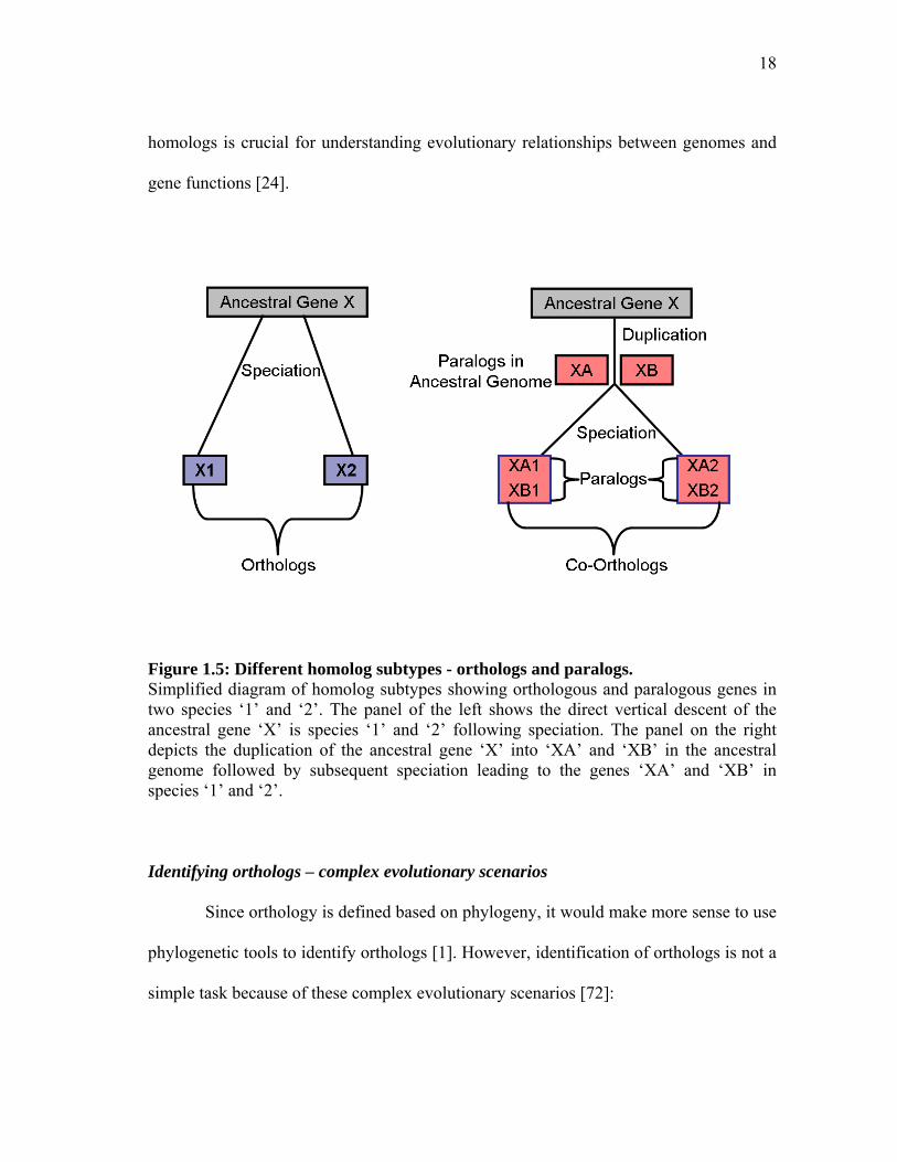
Homologs: orthologs and paralogs
Homologs are of two types: orthologs and paralogs [70, 71]. Orthologs are
homologs that have arisen because of speciation events whereas paralogs are homologs
hat have arisen because of gene duplication events. Figure 1.5 depicts a simplified
diagram of homolog subtypes showing orthologous and paralogous genes in two species
‘1’ and ‘2’. These definitions were first introduced by Walter Fitch in 1970. Orthologs
are evolutionary counterparts derived from a single ancestral gene in the last common
ancestor of the species being compared; paralogs are homologous genes evolved through
duplication within the same (perhaps ancestral too) genome.
Function constraints for orthologs and paralogs
Orthologs are under strict evolutionary constraints and this makes them perform
the same function as long as the function remains essential for survival or at least confers
a substantial selective advantage to its bearers [24, 72]. On the other hand, once paralogs
emerge as a result of gene duplication, the pressure of purifying selection decreases for
the paralog(s), and they acquire new functions [73]. In some sequenced genomes,
substantial fractions (25 to 80%) of genes belong to families of paralogs [74-76] which
reflects diversification of function via duplications at different stages of evolution.
The greater likelihood of orthologs retaining the same ancestral function makes a
strong case for identifying and using orthologs for function predictions and annotation
transfer. Doing so increases the reliability of the transferred functional annotations. The
advent of genomics has reinforced the fact that distinction between the two types of
18
homologs is crucial for understanding evolutionary relationships between genomes and
gene functions [24].
Figure 1.5: Different homolog subtypes - orthologs and paralogs. Simplified diagram of homolog subtypes showing orthologous and paralogous genes in two species ‘1’ and ‘2’. The panel of the left shows the direct vertical descent of the ancestral gene ‘X’ is species ‘1’ and ‘2’ following speciation. The panel on the right depicts the duplication of the ancestral gene ‘X’ into ‘XA’ and ‘XB’ in the ancestral genome followed by subsequent speciation leading to the genes ‘XA’ and ‘XB’ in species ‘1’ and ‘2’. Identifying orthologs – complex evolutionary scenarios
Since orthology is defined based on phylogeny, it would make more sense to use
phylogenetic tools to identify orthologs [1]. However, identification of orthologs is not a
simple task because of these complex evolutionary scenarios [72]:

19
1. when duplication precedes speciation, each of the paralogs gives rise to a distinct
line of orthologous descent;
2. when duplication occurs in one or both lineages independently after speciation,
this is referred to as lineage-specific gene expansion, and leads to a situation
where one-to-one orthologous relationship cannot be delineated;
3. when genes in certain lineages are lost during evolution, this phenomenon is
referred to as lineage-specific gene loss. In such cases, genes which appear to be
orthologs might actually be paralogs.
Complete phylogenetic analysis of all groups of homologous genes helps
decipher true orthologous relationships [24]; however, phylogenetic analysis is
extremely labor-intensive and time-consuming.
It becomes imperative that methods need to be developed to make the distinction
between orthologs and paralogs. The problem gets confounded with large gene families
that have many paralogous members within a species. In such a scenario, the difficulty
lies in identifying the orthologs which are more likely to have conserved function.
In the next section, I describe how phylogenetic analysis can be used to predict
function, and discuss the pros and cons of this approach.
Function prediction using phylogenetic methods
Incorporating an evolutionary perspective to comparative biology involves going
beyond cataloguing similarities and differences between sequences and trying to
20
understand why those similarities and differences came to be [1]. Phylogenomics
combines evolutionary and genomic analysis into a single composite approach [1].
Phylogenomic inference of protein function involves inferring the function of a protein
in the larger context of a protein family [1, 39, 53, 77].
Margaret Dayhoff [78], defines protein family as a group of proteins that perform
similar biochemical functions; the pairwise identity between any two proteins in a
protein family is >50%. However, it is now accepted that all detectable homologs are
members of the same protein family. Coding portions of the genome are organized
hierarchically as gene/protein families [79, 80]; these families are further subdivided into
groups representing distinct subfamilies that have similar functions [32, 53, 60, 77, 81,
82]. A protein family comprises proteins with the same function in different organisms
but may also include proteins derived from gene duplications and rearrangements [83] in
the same organism. Function prediction methods that utilize the protein family approach
include the PANTHER system [84, 85], TIGRfams [86], and some models in PFAM
[87].
To most reliably infer the function of a protein in the larger context of protein
family, protein families should be divided into groups containing orthologs and paralogs
representing distinct subfamilies. In the phylogenomic approach, a phylogenetic tree
involving the different members of the protein family is obtained; the tree topology is
then analyzed and the phylogenetic information encoded in the subfamily (or subtree)
structure is used to infer likely functions for the uncharacterized members of the protein
family. Uncharacterized genes can be assigned predicted function based on the
21
subfamily in which they are placed as function is conserved within orthologous
subfamilies [32, 39, 53, 77, 82]. It is only recently that methods have been developed to
allow high throughput placement of query genes into phylogenetic groups [88-90].
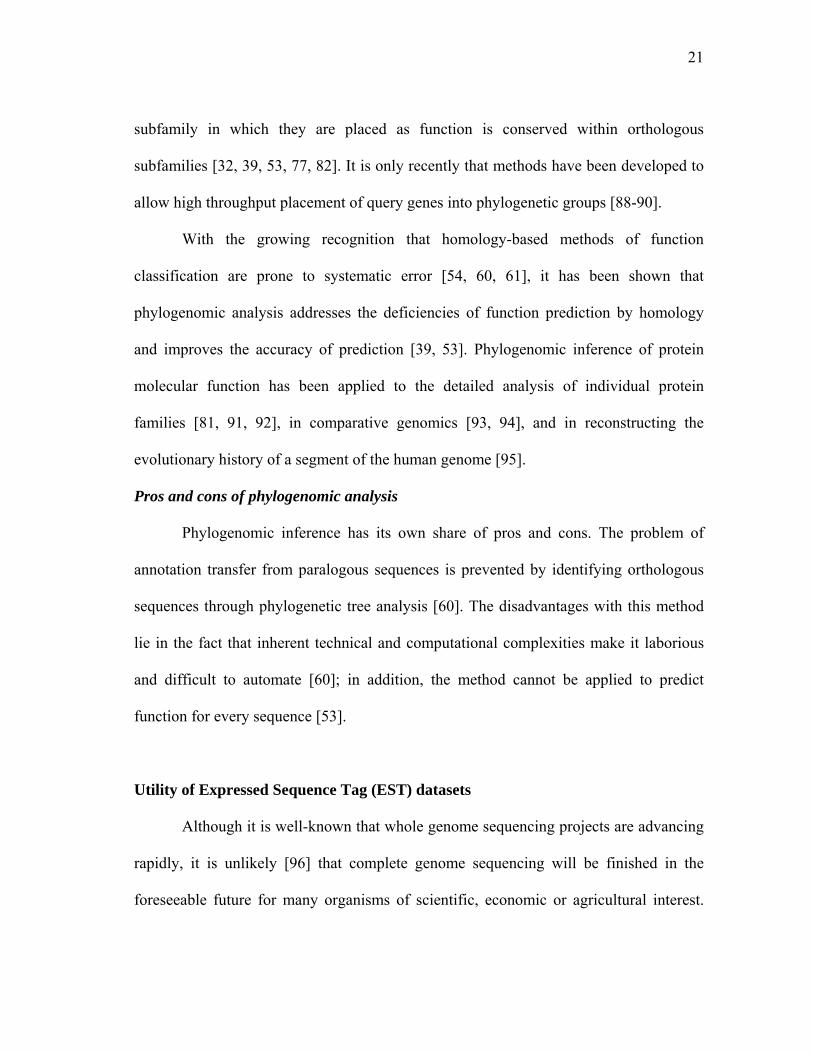
With the growing recognition that homology-based methods of function
classification are prone to systematic error [54, 60, 61], it has been shown that
phylogenomic analysis addresses the deficiencies of function prediction by homology
and improves the accuracy of prediction [39, 53]. Phylogenomic inference of protein
molecular function has been applied to the detailed analysis of individual protein
families [81, 91, 92], in comparative genomics [93, 94], and in reconstructing the
evolutionary history of a segment of the human genome [95].
Pros and cons of phylogenomic analysis
Phylogenomic inference has its own share of pros and cons. The problem of
annotation transfer from paralogous sequences is prevented by identifying orthologous
sequences through phylogenetic tree analysis [60]. The disadvantages with this method
lie in the fact that inherent technical and computational complexities make it laborious
and difficult to automate [60]; in addition, the method cannot be applied to predict
function for every sequence [53].
Utility of Expressed Sequence Tag (EST) datasets
Although it is well-known that whole genome sequencing projects are advancing
rapidly, it is unlikely [96] that complete genome sequencing will be finished in the
foreseeable future for many organisms of scientific, economic or agricultural interest.

22
For most eukaryotic organisms, the complete genome sequence is not available [97], and
sequencing of Expressed Sequence Tags (ESTs) remains the primary tool for functional
genomics approaches.
An EST is a tiny portion of an entire gene [8, 98]; usually about 200 to 500
nucleotides long and is representative of the genes expressed in the tissue at the point of
cDNA library construction. ESTs are obtained by random sequencing of cDNA copies of
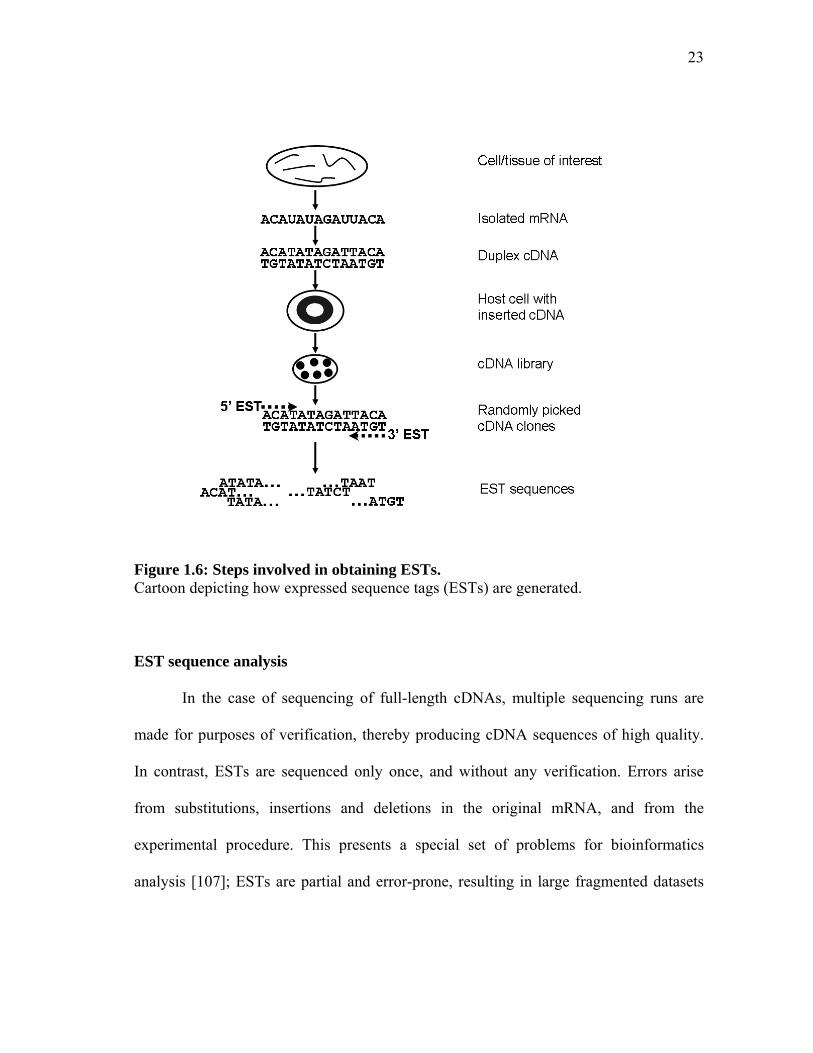
mRNA sequences available (Figure 1.6); the utility of EST projects comes by repeatedly
sequencing clones from a given library to generate many sequence tags as they provide
an opportunity to understand the diversity of genes and the roles they play [99, 100]. The
utility of ESTs is illustrated by the phylogenetic diversity of organisms represented in
dbEST [101, 102], the NCBI’s EST database. As of Sep 2008, there are 55, 796, 748
ESTs deposited in dbEST from thousands of organisms.
EST analysis is a highly cost effective gene discovery method [8, 97, 98, 103]
and EST datasets represent an important resource for comparative and functional
genomics studies [104-106]. In the absence of completed genomes, ESTs help address
these questions:
1. What genes are there in the organism? and
2. What roles do they play?
23
Figure 1.6: Steps involved in obtaining ESTs. Cartoon depicting how expressed sequence tags (ESTs) are generated. EST sequence analysis
In the case of sequencing of full-length cDNAs, multiple sequencing runs are
made for purposes of verification, thereby producing cDNA sequences of high quality.
In contrast, ESTs are sequenced only once, and without any verification. Errors arise
from substitutions, insertions and deletions in the original mRNA, and from the
experimental procedure. This presents a special set of problems for bioinformatics
analysis [107]; ESTs are partial and error-prone, resulting in large fragmented datasets
24
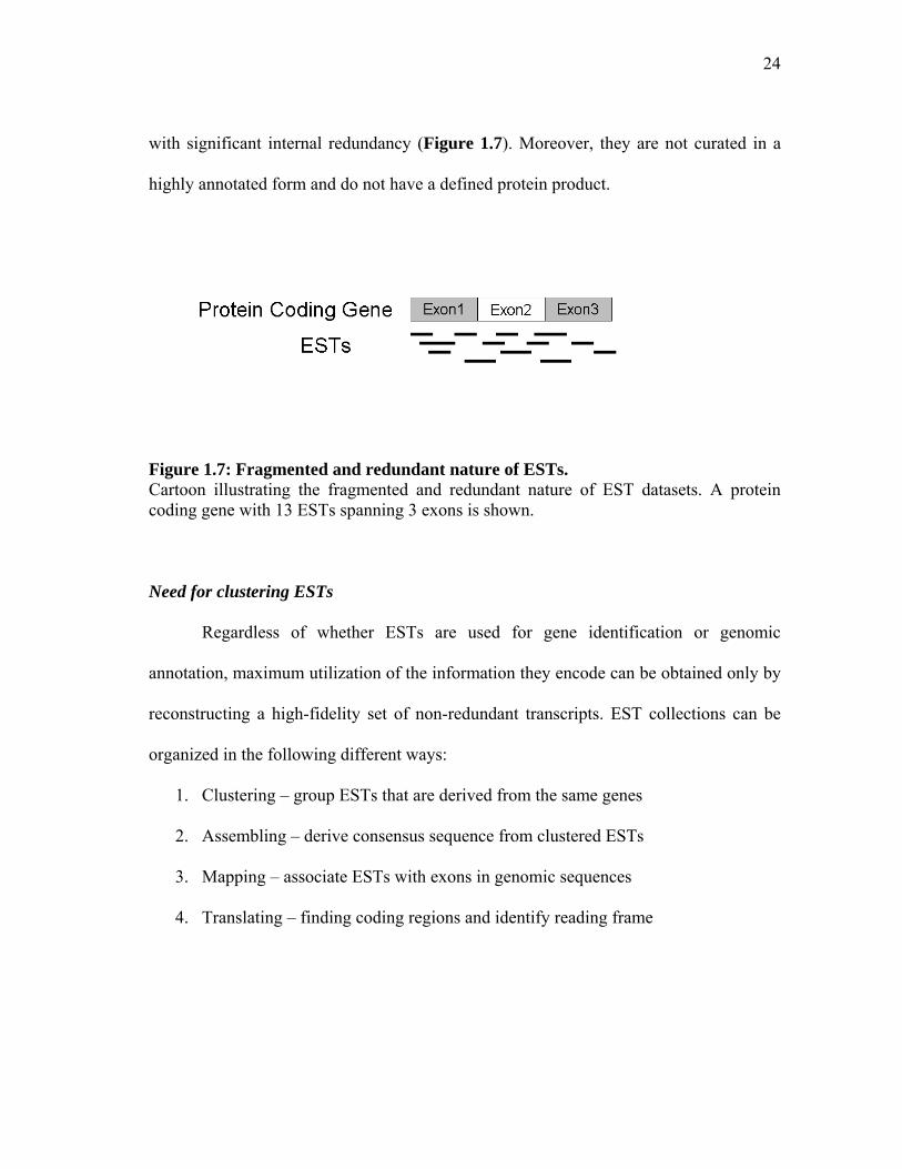
with significant internal redundancy (Figure 1.7). Moreover, they are not curated in a
highly annotated form and do not have a defined protein product.
Figure 1.7: Fragmented and redundant nature of ESTs. Cartoon illustrating the fragmented and redundant nature of EST datasets. A protein coding gene with 13 ESTs spanning 3 exons is shown. Need for clustering ESTs
Regardless of whether ESTs are used for gene identification or genomic
annotation, maximum utilization of the information they encode can be obtained only by
reconstructing a high-fidelity set of non-redundant transcripts. EST collections can be
organized in the following different ways:
1. Clustering – group ESTs that are derived from the same genes
2. Assembling – derive consensus sequence from clustered ESTs
3. Mapping – associate ESTs with exons in genomic sequences
4. Translating – finding coding regions and identify reading frame
25
In the clustering step, ESTs are grouped on the basis of sequence similarity into
clusters; the similarity threshold is set very high (>95%) and the comparisons are made
over a specified window size. The clustered ESTs are then assembled where the
assembly program aligns the EST sequences within a cluster and generates a contiguous
overlapping sequence (or EST contig), or a singleton might arise when the EST(s) could
not be grouped owing to their low similarity to other ESTs. The singletons may represent
genes from rare mRNAs where only a single mRNA is available for the expressed gene,
or may be a result of contamination or poor quality sequence. The contig is a consensus
sequence of several ESTs and is more reliable than the individual ESTs, thereby
reducing the effects of errors. The contigs are consensus sequences having improved
sequence quality [100]. Clustering and assembly of ESTs has numerous advantages,
including, but not limited to, the following:
1. function predictions are significantly improved [97] using the EST consensus
sequences coming from the clustering and assembly pipeline; and
2. clustered EST consensus sequences reduce the search space for similarity
searches and help obtain an accurate estimate of the number of genes.
What is an EST cluster?
An EST cluster contains fragmented EST and (if known) gene sequence data that
has been consolidated and indexed by gene(s) or transcript isoform. In doing so, all
expressed data pertaining to a single gene or isoform exists within a single index class
[100]. Accurate clustering of ESTs requires a strategy that clusters members based on
verifiable information – sequence similarity often being the method of choice.
26
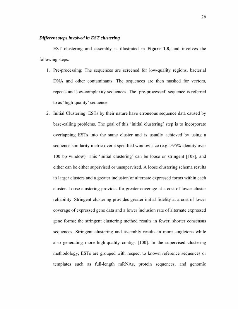
Different steps involved in EST clustering
EST clustering and assembly is illustrated in Figure 1.8, and involves the
following steps:
1. Pre-processing: The sequences are screened for low-quality regions, bacterial
DNA and other contaminants. The sequences are then masked for vectors,
repeats and low-complexity sequences. The ‘pre-processed’ sequence is referred
to as ‘high-quality’ sequence.
2. Initial Clustering: ESTs by their nature have erroneous sequence data caused by
base-calling problems. The goal of this ‘initial clustering’ step is to incorporate
overlapping ESTs into the same cluster and is usually achieved by using a
sequence similarity metric over a specified window size (e.g. >95% identity over
100 bp window). This ‘initial clustering’ can be loose or stringent [108], and
either can be either supervised or unsupervised. A loose clustering schema results
in larger clusters and a greater inclusion of alternate expressed forms within each
cluster. Loose clustering provides for greater coverage at a cost of lower cluster
reliability. Stringent clustering provides greater initial fidelity at a cost of lower
coverage of expressed gene data and a lower inclusion rate of alternate expressed
gene forms; the stringent clustering method results in fewer, shorter consensus
sequences. Stringent clustering and assembly results in more singletons while
also generating more high-quality contigs [100]. In the supervised clustering
methodology, ESTs are grouped with respect to known reference sequences or
templates such as full-length mRNAs, protein sequences, and genomic

27
sequences. In unsupervised clustering, ESTs are grouped without using any
reference sequences.
3. EST Assembly: Once the ‘initial clustering’ is done, a multiple sequence
alignment for each cluster is generated to obtain a ‘consensus sequence’ and/or
singletons.
Figure 1.8: Cartoon illustrating EST clustering and assembly. In the figure, clustering of 11 ‘High quality’ EST sequences results in 11 ESTs getting grouped into 3 clusters and the remaining 2 ESTs are singletons. The assembly process results in 5 EST consensus sequences - 3 EST contigs and 2 singletons. Comparison of the existing EST clustering systems
The aim of EST clustering is to generate a cluster of ESTs that share a transcript
or the gene parent. Systems that are commonly used and have broad acceptance include
28
TGI (TIGR Gene Indices) [109], NCBI’s UniGene [110, 111] and Sequence Tag
Alignment Consensus Knowledgebase (STACK) [112] from South African National
Bioinformatics Institute (SANBI). (Note: TGI is now known as DFCI Gene Indices or
DGI; DFCI denotes the Dana-Farber Cancer Institute). These three systems share an
overall approach, but differ in the choice of algorithms used, reconstruction aims and
coverage of transcript diversity. The three systems perform a similar pre-processing step
that screens out vector, repeat, and low-complexity sequences. Each system differs in the
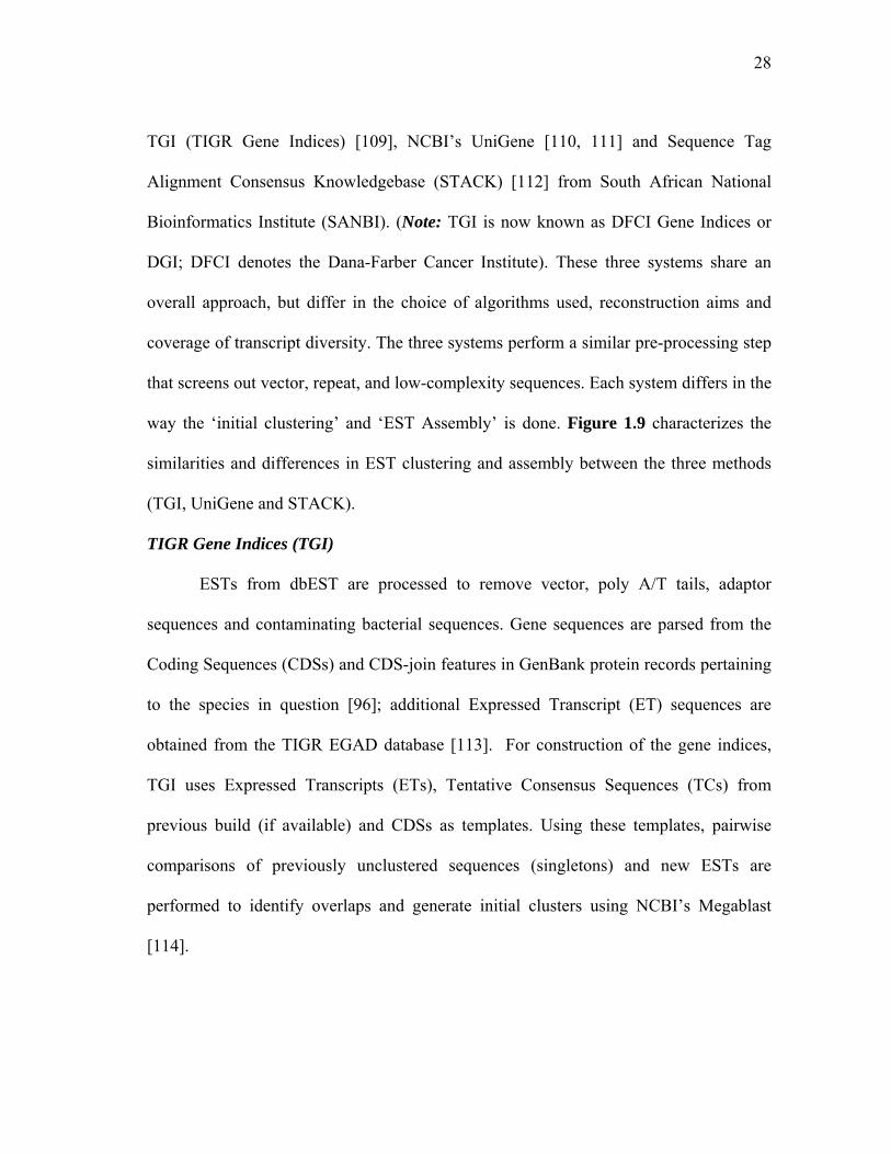
way the ‘initial clustering’ and ‘EST Assembly’ is done. Figure 1.9 characterizes the
similarities and differences in EST clustering and assembly between the three methods
(TGI, UniGene and STACK).
TIGR Gene Indices (TGI)
ESTs from dbEST are processed to remove vector, poly A/T tails, adaptor
sequences and contaminating bacterial sequences. Gene sequences are parsed from the
Coding Sequences (CDSs) and CDS-join features in GenBank protein records pertaining
to the species in question [96]; additional Expressed Transcript (ET) sequences are
obtained from the TIGR EGAD database [113]. For construction of the gene indices,
TGI uses Expressed Transcripts (ETs), Tentative Consensus Sequences (TCs) from
previous build (if available) and CDSs as templates. Using these templates, pairwise
comparisons of previously unclustered sequences (singletons) and new ESTs are
performed to identify overlaps and generate initial clusters using NCBI’s Megablast
[114].

29
Figure 1.9: Comparison of the EST clustering steps of UniGene, TIGR and STACK. Cartoon depicting the different steps in the EST clustering pipeline used by existing EST clustering systems like UniGene, TIGR and STACK. Used with permission from Dr. Lorenzo Cerutti [115], Swiss Institute of Bioinformatics. UniGene does not perform an assembly of the initial ‘EST clusters’; instead each cluster is represented by the longest sequence. STACK concentrates on human sequences and differs from TIGR and UniGene by not using sequence similarity to cluster ESTs. Both STACK and TIGR assemble the initial EST clusters to generate consensus sequences and singletons.
Sequences are grouped into the same cluster if they have ≥ 95% identity over
lengths greater than 40 bases and have < 20 bases mismatch at either end [116]. The
resulting clusters are assembled by Paracel Transcript Assembler [117] to obtain
Tentative Consensus Sequences, which represent the underlying mRNA transcripts.
30
These TCs are then annotated using information in GenBank and/or protein homology
[116].
The TGI clustering methodology results in shorter consensus sequences [115]
compared to UniGene and STACK. TGI tightly groups highly related sequences,
separates splice variants into different clusters and discards under-represented or
divergent sequences.
UniGene
Clusters are built from genes and mRNAs in GenBank. ESTs are initially
clustered using GenBank CDSs and mRNAs as ‘seed’ sequences. ESTs that join two
clusters of mRNA/genes are discarded. To minimize the frequency of multiple clusters
being identified for a single gene, UniGene clusters are required to contain at least one
sequence carrying readily identifiable evidence of having reached the 3′ terminus. In
other words, UniGene clusters must be anchored at the 3′ end of a transcription unit.
Hence, any resulting cluster without a polyadenylation signal or not having at least two
3’ ESTs is discarded [111].
UniGene clusters ESTs similar to the ‘seed’ sequence and categorizes the clusters
into “highly similar” to the seed (defined as >90% identity in the aligned region),
“moderately similar” (70-90% identity), or “weakly similar” (<70% identity) [118].
UniGene uses pairwise comparisons at varying levels of stringency to group sequences,
placing closely related and alternatively spliced transcripts into one cluster [115].
UniGene per se does not perform an ‘EST cluster assembly’ of the generated clusters
and consensus sequences are not made; instead each cluster is represented by the longest

31
sequence. In summary, UniGene does not actually reconstruct transcripts but instead
attempts to define their cluster membership based on NCBI data.
A common error in UniGene is incorrect clone joining, where irrespective of
sequence overlap, 5’ and 3’ ESTs are placed in the same cluster if they share a parent
clone. Another drawback of the sequence comparison method in UniGene results in
unrelated clusters being joined together by chimerism and other artifacts.
STACK
STACK concentrates on human data and an initial sub-partitioning step is
performed where human ESTs from GenBank are grouped in tissue-based categories.
After masking for repeats, vectors and other contaminants, the resulting ‘high quality’
ESTs are subject to a ‘loose’ clustering approach using d2_cluster [119]. The
‘d2_cluster’ approach is not based on alignments; instead it performs comparisons via
non-contextual assessment of the compositions and multiplicity of words within each
sequence. The ‘d2_cluster’ looks for the co-occurrence of n-length words (n=6) within
window sizes of 150 bases having at least 96% identity.
In a stringent assembly process, the clusters from ‘d2_cluster’ are initially
assembled by PHRAP [120]. CRAW [121] is used to generate consensus sequences with
maximized length and CRAW partitions a cluster into sub-ensembles if ≥50% of a 100
base window differs significantly from the remaining sequences in the cluster. The
different sub-ensembles are ranked according to the number of assigned sequences and
number of called bases for each sub-ensemble.

32
STACK places highly related sequences into the same cluster, as well as
sequences related by rearrangements or alternate splicing. STACK generates longer
consensus sequences and integrates 30% more ESTs than UniGene and produces longer
consensus sequences compared to TGI [115].
Figure 1.10 is a cartoon that depicts the differences in stringency levels in the
EST clustering pipeline used by the existing EST clustering schemes like UniGene,
TIGR and STACK.
Figure 1.10: Comparison of the EST clustering stringency levels of TIGR, UniGene and STACK. Cartoon depicting the stringency differences between the three EST clustering methods -TIGR, UniGene and STACK. Used with permission from Dr. Lorenzo Cerutti [115], Swiss Institute of Bioinformatics. TIGR, the most stringent amongst all the methods [115], tightly groups highly related sequences and separates splice variants into different clusters. Both UniGene and STACK place highly related and alternatively spliced transcripts in the same cluster. However, STACK [115] generates longer consensus sequences and integrates 30% more ESTs than UniGene and produces longer consensus sequences compared to TIGR Gene Indices.
33
Function predictions using EST datasets
In the absence of completely sequenced genomes and the accompanying high-
quality annotations, one can use Expressed Sequence Tag (EST) datasets to gain insights
about the functions encoded in the genome by first determining what genes are there in
the organism and then finding out what roles they play. Annotated EST datasets address
the need of connecting ESTs with the functions they encode.
Need for protein sequence comparisons using ESTs
DNA sequences produced by single-pass EST sequencing are of lower quality
than traditional “finished” GenBank sequences and the EST sequences are more likely to
contain frameshifts when translated to protein. These frameshift errors are troublesome
in searches with single-pass EST sequences as these regions are likely to be protein-
coding, which are much more effectively identified by protein sequence comparison than
by DNA sequence comparison [15]. In addition, the evolutionary look-back time is
more than doubled by protein sequence comparisons as against DNA sequence
comparisons [122, 123]; hence it makes sense to compare protein sequences if the
sequences encode proteins. One of the approaches that has been proved invaluable in
comparative genomics and computational biology in general is that whenever distant
relationships are involved and sensitivity is an issue, protein sequences rather than
nucleotide sequences should be compared directly [24].
Function predictions with EST datasets using sequence homology based approach
A common strategy for obtaining function annotations for EST datasets is to
search well-annotated proteomes using BLASTX/FASTX (translated DNA query against
34
a protein database), obtain information about the homolog with the “best hit” and to
transfer the annotations of the “best hit” match to the EST consensus sequence [104-
106].
There are limitations of subjecting EST libraries to whole proteome searches due
to the short length of the translated EST sequence (the equivalent of 30 to 150 amino
acids) which would match only part of the protein; for example, a protein domain or part
of it [97]. The accuracy of the computational function predictions is significantly
improved [97] when EST consensus sequences are used instead of the individual ESTs.
Function predictions with EST datasets using a phylogeny based approach
ESTs can be coarsely grouped based on their matches to proteins, and subject to
clustering and assembly to obtain EST gene families. The EST consensus sequences in
these EST gene families can be grouped with other proteins in the family and subject to
a phylogenomic inference pipeline. The topologies of the phylogenetic trees can be
analyzed to infer likely functions for the EST consensus sequences based on orthologous
proteins.
Work in this dissertation
In this dissertation, Bos taurus and Sus scrofa ESTs were clustered and
assembled using vertebrate proteins from Ensembl as the framework. This clustering
was performed as part of the TAMUClust pipeline, a new EST clustering method
developed by Dr. Elsik. The performance of TAMUClust was compared to currently
used EST clustering schemes (TGI/UniGene) by using Bos taurus EST clusters from the

35
respective data sources and designing cluster equivalence comparison studies (Chapter
II). The Bos taurus and Sus scrofa EST consensus sequences obtained were annotated
by transferring annotations of the Ensembl vertebrate protein(s) following sequence
homology searches and phylogenetic analysis (Chapter III and Chapter IV).
36
CHAPTER II
VALIDATION OF TAMUClust - A NOVEL EST CLUSTERING METHODOLOGY
SYNOPSIS
Expressed Sequence Tags (ESTs) are single pass sequence reads from randomly
selected cDNA clone. They serve as a viable alternative to the genome sequencing of
many organisms as they provide a high-throughput method to sample an organism’s
transcriptome and identify expressed genes. ESTs contain high error rates, and the
information encoded is often fragmented and redundant. Therefore, EST sequences are
clustered into groups likely to have been derived from the same genes and this process
improves the quality of meaningful information that can be derived from ESTs.
Chimerism, the single largest contributor to EST misassemblies, can be avoided if ESTs
are initially grouped into clusters based on their matches to proteins, and then subject to
clustering and assembly. TAMUClust is a new EST clustering method that uses the
protein framework to cluster ESTs. The TAMUClust Bos taurus EST clusters are
compared with the Bos taurus EST clusters from TIGR Gene Indices (TGI), the current
method of choice in EST clustering. Two types of comparisons are made: (i)
determining cluster equivalence for TAMUClust/TGI using bovine genome aligned EST
clusters as the reference and (ii) determining how many genes are represented in
TAMUClust/TGI using predicted bovine transcripts as the reference. Results indicate
that the TAMUClust method compares well with TGI.

37
BACKGROUND
The utility of Expressed Sequence Tags (ESTs)
Expressed Sequence Tags (ESTs) are single pass sequence reads from randomly
selected cDNA clones and provide a high-throughput cost-effective method to sample an
organism’s transcriptome [8, 98]. ESTs are short (usually 200-500 bases in length),
unedited sequence reads and represent a tiny portion of a protein coding gene. ESTs
offer a rapid and inexpensive route to gene discovery [8], reveal expression and
regulation data [124], and highlight gene sequence diversity and alternative splicing
[125]. EST datasets have been utilized as an alternative to the genome sequencing of
many organisms, earning the label, the ‘poor man’s genome’ [126].
Need for EST clustering
ESTs are sequenced only once, and without any verification. The high-volume
and the high-throughput nature of the EST datasets have a lot of downsides – ESTs
contain high error rates with the errors arising from substitutions, insertions and
deletions in the original mRNA, and from the experimental procedure. Maximum
utilization of the information enoded in ESTs can be obtained by clustering ESTs into
groups that have been derived from the same genes, resulting in a high-fidelity set of
non-redundant transcripts. Sequence identity between the cluster members is the method
of choice in clustering ESTs.
38
Need of EST clustering using a protein family framework and associated benefits
Chimeric EST clusters are encountered when ESTs representing different genes
get grouped together in a single cluster. Chimerism is the single largest contributor to
generation of ‘incorrect EST assemblies’ (misassemblies). Chimeric EST clusters can be
eliminated by performing an initial coarse level grouping of ESTs based on their
matches to proteins. In a subsequent step, clustering and assembly of ESTs can be done
to obtain EST gene families. By incorporating a protein framework to cluster ESTs, the
cluster quality can be improved and misassemblies can be minimized.
The need for clustering ESTs using a protein framework lead to the development
of a new EST clustering method called TAMUClust. This method was developed in our
lab by Dr. Elsik.
Description of TAMUClust - a novel EST clustering system
TAMUClust uses a protein framework to cluster and assemble ESTs in a two-
step clustering process.
In the first step, vertebrate proteins are clustered into protein families using a
combination of single-linkage and average-linkage clustering. The protein families
generated are non-redundant, comprehensive set of full-length protein clusters with
homogeneous domain architecture within clusters and the pairwise sequence identity
between any two proteins within each cluster is at least 55%. A total of 219,433 proteins
from the proteomes for Homo sapiens, Mus musculus, Rattus norvegicus, Gallus gallus,

39
Danio rerio, Takifugu rubripes and Tetraodon nigroviridis were obtained from Ensembl
[9] in April 2005; these proteins were distributed across 10,992 protein families.
In the second step, TAMUClust uses the protein families obtained in the previous
step as a framework to group ESTs into gene families using a translated-DNA:protein
search. For ESTs within each family, a DNA:DNA sequence identity metric is used to
build consensus sequences. The protein comparison step incorporated before assembling
ESTs helps identify coding regions and produce reliable protein translations.
Other commonly used EST Clustering systems such as TGI (TIGR Gene
Indices), UniGene, and STACK do not use a protein framework to cluster and assemble
ESTs.
Importance of generating the correct EST clusters
DNA microarrays (DNA chips) allow for simultaneous measurement of
transcription levels for every gene. A DNA microarray is a slide on which an array of
spots has been deposited. Each spot contains many copies of a specified DNA sequence
that has been anchored chemically to the slide surface, with a different DNA sequence
for each spot.
In the long oligonucleotide array, the oligos are usually 60-70 bases long and are
selected for their uniqueness. These are used to profile the gene expression in a genome,
and the oligos may be designed such that there is only one oligo per gene or transcript.
In the absence of completed genomes, ESTs are used to determine what genes
are there in the organism and to design the oligonucleotide probes. In this scenario, it is

40
important to ensure that the transcript reconstruction from ESTs is accurate and non-
redundant. Inaccuracies with EST clustering would result in problems in selecting
sequences for oligonucleotide design. Usually one EST per cluster is selected for oligo
design. Overclustering (i.e. grouping unrelated ESTs) would result in lack of
representation of some genes; underclustering (i.e. splitting same-gene ESTs into
different clusters) would cause multiple oligos to be designed for one gene. Designing
oligonucleotide probes by utilizing ESTs clustered using a protein framework could
minimize probe redundancy and maximize representation of different genes.
Overview of the work in this chapter
TAMUClust is a novel EST Clustering system developed in our lab by Dr. Chris
Elsik. In this method, ESTs are clustered and assembled using a protein framework.
Pilot study
A pilot study was carried out in January 2004 using TAMUClust Bos taurus EST
clusters generated using Ensembl human protein families as a framework. Using the
Qsingle metric, the results of TAMUClust were compared to those obtained with other
commonly used methods like TGI [127] and UniGene [110] for the same set of Bos
taurus ESTs.
For the purposes of our pilot study comparison analyses, the reference
classification was either the Bos taurus Gene Indices (BTGI) obtained from TGI or the
UniGene Bos taurus EST clusters whereas the query classification refers to the
TAMUClust Bos taurus EST clusters. However, this is not to say that the TGI or

41
UniGene is “correct”. They were used as “references” in the pilot study as they are the
existing methods of choice in EST clustering.
Results from the pilot study indicated that TAMUClust performance compares
well with TGI and UniGene. We chose not to include further comparisons of
TAMUClust with UniGene as the clustering methodology of TAMUClust is similar to
TGI than UniGene.
Comparisons with assembled genome
In August 2006, the third version of the bovine genome assembly, Btau_3.1 was
released with a 7.15X coverage [10, 11]. The availability of this high quality bovine
assembly came in handy to compare the performance of TAMUClust Bos taurus EST
clusters against the Bos taurus Gene Indices (BTGI) obtained from TGI/DGI [128] by
using bovine ESTs aligned to the bovine genome assembly 3.1 as the reference (gold
standard). Results from this analysis indicated that the TAMUClust performance was
comparable to TGI, and marginally better than TGI.
Comparisons using predicted gene models
In July 2008, the fourth version of the bovine genome assembly, Btau_4.0 was
released. Two kinds of ‘megablast’ analyses were carried out by using transcripts from
the Bos taurus Ensembl Release 50 [129] as the reference (Gold standard).
In the first analysis, TAMUClust/BTGI bovine EST consensus sequences were
used as the query and searched against the bovine transcripts in Ensembl Release 50
(July 2008). The performance of TAMUClust and BTGI was compared by obtaining
42
statistics on the Ensembl transcripts identified or missed by the respective EST
clustering methods. More specifically, this analysis was designed to address the question
“Does TAMUClust gain anything by including singletons in its gene indices”. Since
TAMUClust used a protein framework to cluster and assemble ESTs, TAMUClust also
included singletons in the gene indices (consensus sequences) it generated where these
singletons had a statistically significant sequence similarity to a homologous protein.
BTGI performs a nucleotide-nucleotide comparison to cluster and assemble ESTs, and
discards ESTs that do not match the clustering criteria. As a result, the gene indices
generated by BTGI were devoid of singletons. Based on the bovine transcripts identified
by TAMUClust singletons and missed by BTGI consensus sequences, one can conclude
that TAMUClust singletons were not clustering artifacts and TAMUClust singletons
should be included in the final gene indices.
In the second analysis, the bovine transcripts in Ensembl Release 50 were used as
the query and searched against TAMUClust/BTGI bovine EST consensus sequences.
This analysis was designed to obtain an estimate of the transcript coverage in
TAMUClust and BTGI by obtaining a count of the number of predicted transcripts that
match TAMUClust/BTGI consensus sequences. Results from this study indicated that
the number of predicted transcripts that match TAMUClust/BTGI consensus sequences
were almost the same.

43
MATERIALS AND METHODS
Qsingle - cluster equivalence comparison metric
Gracy and Argos [130] have developed a method that helps evaluate the quality
of a new classification scheme B in terms of a reference classification A for the same
dataset X. Here, the number of True Positives (TP) is given by (|a ∩ b|-1), that of False
Positives (FP) is given by |b\a|, and that of False Negative (FN) is given by |a\b|. In this
method, each class a ∈A is associated with the group b ∈B which maximizes the
quantity TP-FP-FN. Quality is defined by the percentage of the true positives
(100*TP/TP+FP+FN). The underlying meanings of the conventions used in the
comparison metric described above are as follows:
1. a ∩ b refers to the intersection of ‘a’ and ‘b’ – in other words, it refers to the
number of members common to ‘a’ and ‘b’.
2. b\a refers to members present in ‘b’ and absent from ‘a’.
3. a\b refers to members present in ‘a’ and absent from ‘b’.
This method of comparing the quality of a new classification in terms of a
reference classification as indicated by the mutual agreement of the two classification
schemes has been used in the ProtoMap [131] classification evaluation. The ProtoMap
authors have termed this ‘Quality Index’ as ‘Qsingle’ and we also use the same term in our
cluster equivalence comparison analyses.

44
Qsingle calculation
The different statistical parameters (tp, fp, fn) and the Qsingle metric were obtained
using the following steps:
1. identify the common ESTs in both datasets – the new classification scheme ‘B’
and the reference classification scheme ‘A’.
2. for every EST ‘E’ in ‘B’ do;
3. obtain the cluster_id in A and B for the cluster that has ‘E’. Lets call them
cluster_id_A and cluster_id_B
4. obtain all the other ESTs in cluster_id_A and cluster_id_B. Lets denoted the
members as cluster_id_A_members and cluster_id_B_members
5. identify the cluster_id_A associated with cluster_id_B that maximizes the
quantity TP-FP-FN
6. Qsingle % TP = (100* TP/TP+FP+FN)
7. Qsingle % FP = (100* FP/TP+FP+FN)
8. Qsingle % FN = (100* FN/TP+FP+FN)
9. The different Qsingle indices (Qsingle %TP, Qsingle %FP and Qsingle %FN) are
segregated into different bins, for e.g. (0 to 10%, 10 to 20%, and so on).
Methods used in the pilot study
Pilot study: TAMUClust Bos taurus EST clusters
Bos taurus ESTs were downloaded from dbEST [101] in March 2003, and after
quality control (removal of low quality sequence, untrimmed vector, linker, ribosomal,
45
mitochondrial, poly A/T tails), 313,503 ‘High Quality’ ESTs were obtained. These
ESTs were passed through the TAMUClust pipeline which resulted in 37,025 EST
consensus sequences (15,157 contigs and 21,868 singletons).
Pilot study: Bos taurus EST clusters from TIGR Gene Indices
In Sep 2003, Bos taurus EST clusters were obtained from Bos taurus Gene
Indices (BTGI) Release 9 at The Institute of Genome Research (TIGR) Gene Indices
database [127]. This BTGI release had 268,328 ESTs distributed in 34,976 clusters.
Pilot study: Bos taurus EST clusters from UniGene
In Sep 2003, Bos taurus EST clusters (UniGene Build 49) were obtained from
UniGene [110]. This UniGene Build had 209,550 ESTs distributed in 18,153 clusters.
Note: The individual ESTs and also the number of ESTs in BTGI/UniGene are
different from what it is in TAMUClust because of the different dates on which the
respective sources (TAMUClust/BTGI/UniGene) downloaded the ESTs from dbEST.
Pilot study: Qsingle indices
Qsingle quality comparisons as described above were performed by means of these
two comparisons:
i. TAMUClust Bos taurus EST clusters versus BTGI Bos taurus EST clusters using
119,047 ESTs common to both datasets.
ii. TAMUClust Bos taurus EST clusters versus UniGene Bos taurus EST clusters
using 97,245 ESTs common to both datasets.
46
Methods used in comparisons with the assembled genome (Gold standard
comparisons)
Gold standard comparisons: TAMUClust Bos taurus EST clusters
Bos taurus ESTs were downloaded from dbEST [101] in April 2005, and after
quality control (removal of low quality sequence, untrimmed vector, linker, ribosomal,
mitochondrial, poly A/T tails), 308,132 ‘High Quality’ ESTs were obtained. These
ESTs were passed through the TAMUClust pipeline which resulted in 46,731 EST
consensus sequences (24,665 contigs and 22,066 singletons).
Gold standard comparisons: BTGI (Bos taurus Gene Indices) EST clusters
In March 2007, the file “BTGI.release_12.zip” was obtained from the ftp site
[132] of the Bos taurus Gene Indices at DGI [133]. The file was decompressed and the
resulting files were parsed to obtain information on the BTGI clusters and the constituent
ESTs. The BTGI dataset had 955,223 ESTs clustered into 90,392 EST clusters.
Note: The individual ESTs and also the number of ESTs in BTGI would be
different from what it is in TAMUClust depending on the dates on which the respective
sources (TAMUClust/BTGI) downloaded the ESTs from dbEST.
Gold standard comparisons: bovine genome aligned EST clusters
Bos taurus ESTs (1,165,913 ESTs) were downloaded from the NCBI dbEST
database [101] in April 2007. Using the Splign alignment and splice modeling tool [134]
and %identity >95%, bovine ESTs were aligned to the third version of the bovine
assembly (Assembly 3.1, 7.1X coverage [10, 11]). Alignments were stored as gff3 [135]
files and perl scripts were written to parse the gff3 files to obtain ESTs that have only
47
one alignment location on the genome. Further perl processing was done to identify
overlapping ESTs and grouped into clusters. The bovine genome aligned EST clusters
constitute the reference classification (or the gold standard dataset); they comprised of
975,728 ESTs in 44,579 clusters.
Qsingle indices in the gold standard comparisons
Qsingle quality comparisons as described above were performed by means of these
comparisons:
1. One to one comparison of TAMUClust Bos taurus EST clusters and gold
standard dataset using 209,645 ESTs common to both datasets.
2. One to one comparison of BTGI Bos taurus EST clusters and gold standard
dataset using 702,128 ESTs common to both datasets.
3. One to one comparisons of TAMUClust Bos taurus EST clusters vs gold
standard dataset and BTGI Bos taurus EST clusters vs gold standard dataset
using 198,438 ESTs common to all three datasets.
To account for the fact that BTGI Bos taurus EST clusters did not include
singletons whereas TAMUClust clusters included singletons, the above Qsingle analyses
were repeated (henceforth referred to as ‘singleton minus’ analyses) by excluding
singletons from the TAMUClust dataset.
1. Singleton minus one to one comparison of TAMUClust Bos taurus EST clusters
and gold standard dataset using 198,525 ESTs common to both datasets.
48
2. Singleton minus one to one comparisons of TAMUClust Bos taurus EST clusters
vs gold standard dataset and BTGI Bos taurus EST clusters vs gold standard
dataset using 192,920 ESTs common to all three datasets.
Methods used in comparisons with the predicted gene models
Predicted bovine transcripts
The file ‘Bos_taurus.Btau_4.0.50.cdna.all.fa.gz’ was obtained from the Ensembl
ftp site for Bos taurus Ensembl Release 50 [129]. Perl scripts were written to identify the
longest transcript for each gene, and this transcript dataset served as the ‘reference’
dataset in the predicted transcript comparison study. The reference dataset had 21, 722
transcripts.
Megablast analysis I
This analysis was designed to address the question “Does TAMUClust gain
anything by including singletons in its gene indices”. To address this, we used Megablast
[114], and the TAMUClust/BTGI consensus sequences were used as the query and
searched against the ‘reference transcript dataset’ from the Bos taurus Ensembl Release
50 as mentioned above.
The Megablast results were filtered to include only those alignments which were
longer than 100 bases in alignment length and had sequence identity ≥ 95%. Perl scripts
were written to parse the Megablast results in order to obtain information on the
Ensembl transcripts identified or missed by the respective EST clustering methods. We
first determined if there were any Ensembl transcripts that aligned to TAMUClust

49
consensus sequences but were missed by BTGI consensus sequences; from these
TAMUClust hits, we then identified the TAMUClust singletons.
Megablast analysis II
This analysis was designed to identify the extent of coverage of the predicted
bovine transcripts in the TAMUClust and BTGI datasets. To address this, the ‘reference
transcript dataset’ from the Bos taurus Ensembl Release 50 as mentioned above was
used as the query and searched against the TAMUClust/BTGI consensus sequences.
The Megablast results were filtered to include only those alignments which were
longer than 100 bases in alignment length and had sequence identity ≥ 95%. Perl scripts
were written to parse the Megablast results in order to obtain information on the extent
of transcript coverage in the TAMUClust and BTGI datasets using the ‘reference
transcript dataset’.
RESULTS AND DISCUSSION
As an aid to the reader, Table 2.1 details the datasets involved in the various
Qsingle analyses performed in this study and the Table/Figure in which the corresponding
Qsingle analysis is discussed. The gold standard dataset in the Qsingle analyses described
below refers to the bovine genome aligned EST clusters (bovine ESTs aligned to the Bos
taurus Assembly 3.1).

50
Table 2.1: Table detailing the various Qsingle analyses performed and the
Table/Figure in which they appear in this chapter.
Study Type of Qsingle analysis EST datasets used Table/Figure
Pilot study
TAMUClust as query and BTGI
as reference
ESTs common to TAMUClust
and BTGI
Table 2.3,
Figures 2.1 and
2.2
TAMUClust as query and
UniGene as reference
ESTs common to TAMUClust
and UniGene
Table 2.4,
Figures 2.1 and
2.2
Gold standard
(bovine genome
aligned ESTs) study
TAMUClust as query and
bovine genome aligned ESTs
as reference
ESTs common to TAMUClust
and bovine genome aligned
EST clusters
Table 2.7,
Figures 2.3 and
2.4
BTGI as query and bovine
genome aligned ESTs as
reference
ESTs common to BTGI and
bovine genome aligned EST
clusters
Table 2.8,
Figures 2.3 and
2.4
TAMUClust or BTGI as query
and bovine genome aligned
ESTs as reference
ESTs common to TAMUClust,
BTGI and bovine genome
aligned EST clusters
Table 2.9,
Figures 2.5 and
2.6
Singleton minus
analysis I
TAMUClust as query and
bovine genome aligned ESTs
as reference
Excluding TAMUClust
singletons and using ESTs
common to TAMUClust and
bovine genome aligned EST
clusters
Table 2.10,
Figures 2.7 and
2.8
Singleton minus
analysis II
TAMUClust or BTGI as query
and bovine genome aligned
ESTs as reference
Excluding TAMUClust
singletons and using ESTs
common to TAMUClust, BTGI
and bovine genome aligned
EST clusters
Table 2.12,
Figures 2.10
and 2.11
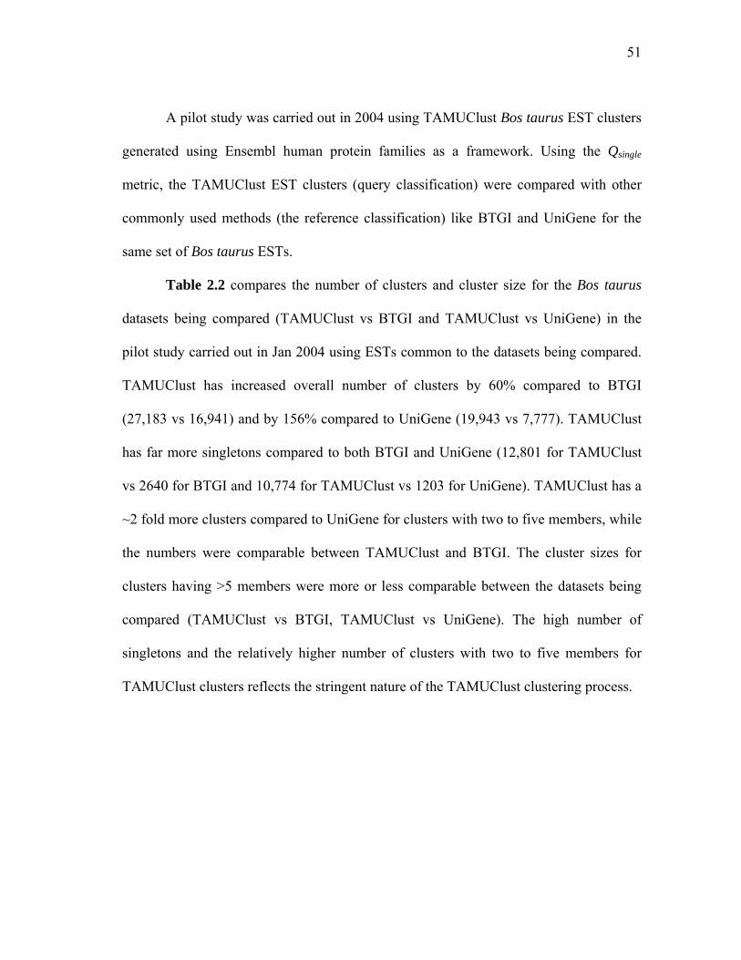
51
A pilot study was carried out in 2004 using TAMUClust Bos taurus EST clusters
generated using Ensembl human protein families as a framework. Using the Qsingle
metric, the TAMUClust EST clusters (query classification) were compared with other
commonly used methods (the reference classification) like BTGI and UniGene for the
same set of Bos taurus ESTs.
Table 2.2 compares the number of clusters and cluster size for the Bos taurus
datasets being compared (TAMUClust vs BTGI and TAMUClust vs UniGene) in the
pilot study carried out in Jan 2004 using ESTs common to the datasets being compared.
TAMUClust has increased overall number of clusters by 60% compared to BTGI
(27,183 vs 16,941) and by 156% compared to UniGene (19,943 vs 7,777). TAMUClust
has far more singletons compared to both BTGI and UniGene (12,801 for TAMUClust
vs 2640 for BTGI and 10,774 for TAMUClust vs 1203 for UniGene). TAMUClust has a
~2 fold more clusters compared to UniGene for clusters with two to five members, while
the numbers were comparable between TAMUClust and BTGI. The cluster sizes for
clusters having >5 members were more or less comparable between the datasets being
compared (TAMUClust vs BTGI, TAMUClust vs UniGene). The high number of
singletons and the relatively higher number of clusters with two to five members for
TAMUClust clusters reflects the stringent nature of the TAMUClust clustering process.
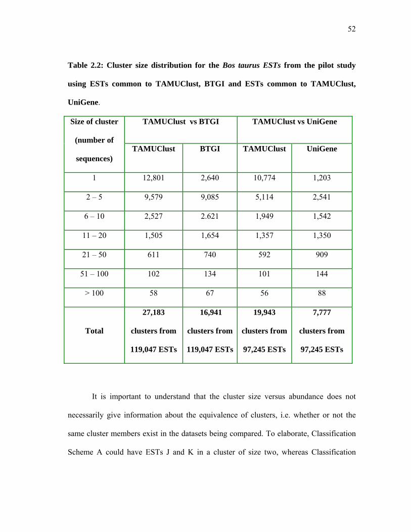
52
Table 2.2: Cluster size distribution for the Bos taurus ESTs from the pilot study
using ESTs common to TAMUClust, BTGI and ESTs common to TAMUClust,
UniGene.
Size of cluster
(number of
sequences)
TAMUClust vs BTGI TAMUClust vs UniGene
TAMUClust BTGI TAMUClust UniGene
1 12,801 2,640 10,774 1,203
2 – 5 9,579 9,085 5,114 2,541
6 – 10 2,527 2.621 1,949 1,542
11 – 20 1,505 1,654 1,357 1,350
21 – 50 611 740 592 909
51 – 100 102 134 101 144
> 100 58 67 56 88
Total
27,183
clusters from
119,047 ESTs
16,941
clusters from
119,047 ESTs
19,943
clusters from
97,245 ESTs
7,777
clusters from
97,245 ESTs
It is important to understand that the cluster size versus abundance does not
necessarily give information about the equivalence of clusters, i.e. whether or not the
same cluster members exist in the datasets being compared. To elaborate, Classification
Scheme A could have ESTs J and K in a cluster of size two, whereas Classification

53
Scheme B could have ESTs K and L in a cluster of size two or have ESTs M and N in a
cluster of size two, with ESTs J and K existing in some other cluster of a different size.
Hence, it is important to first identify the cluster in the different classification schemes
housing the EST under comparison and then compare the members of the clusters
between the two schemes to determine the degree of agreement. In this scenario, we use
the Qsingle metric which evaluates the quality of a new classification scheme B by
comparing it to a reference classification scheme A for the same dataset X.
Interpreting the Qsingle metric
The Qsingle index determines quality based on the percentage of True Positives
(Qsingle %TP), percentage of False Positives (Qsingle %FP) and percentage of False
Negatives (Qsingle %FN) obtained in the analysis. In this method which compares the
performance of a new classification scheme B to a reference classification A, each class
a ∈A is associated with the group b ∈B which maximizes the quantity TP - FP - FN.
The Qsingle %TP, Qsingle %FP and Qsingle %FN values are determined as described in
Materials and Methods.
If the new classification scheme performs just as well as the reference
classification scheme, this would result in 100% TP, 0% FP and 0% FN. However, such
an idealistic situation is rarely encountered. Instead, what is seen is that the different
Qsingle indices have values ranging from 0% to 100%. These indices are then segregated

54
into different bins, for e.g. 0 to 10%, 10 to 20%, and so on, where the cluster abundance
across the different bins is an indicator of the performance of the new classification
scheme when compared to the reference. In such a scenario, interpretation of the
different Qsingle indices give insights about how ‘close’ or ‘similar’ the new classification
scheme is in comparison to the reference classification schemes. Given below are some
of the indicators that signify a “very similar’ performance between the two schemes:
1. A high percentage of clusters in the upper bins (>90%) for the Qsingle %TP
parameter.
2. A high percentage of clusters in the lower bins (<10%) for Qsingle %FP and Qsingle
%FN parameters.
The distribution of the Qsingle indices for the pilot study comparison between
TAMUClust vs BTGI and TAMUClust vs UniGene are detailed in Tables 2.3 and 2.4
respectively.
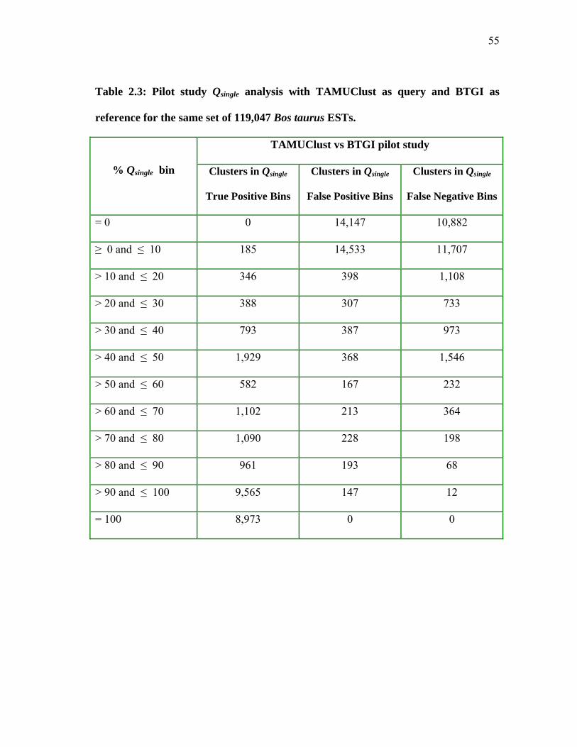
55
Table 2.3: Pilot study Qsingle analysis with TAMUClust as query and BTGI as
reference for the same set of 119,047 Bos taurus ESTs.
% Qsingle bin
TAMUClust vs BTGI pilot study
Clusters in Qsingle
True Positive Bins
Clusters in Qsingle
False Positive Bins
Clusters in Qsingle
False Negative Bins
= 0 0 14,147 10,882
≥ 0 and ≤ 10 185 14,533 11,707
> 10 and ≤ 20 346 398 1,108
> 20 and ≤ 30 388 307 733
> 30 and ≤ 40 793 387 973
> 40 and ≤ 50 1,929 368 1,546
> 50 and ≤ 60 582 167 232
> 60 and ≤ 70 1,102 213 364
> 70 and ≤ 80 1,090 228 198
> 80 and ≤ 90 961 193 68
> 90 and ≤ 100 9,565 147 12
= 100 8,973 0 0

56
Table 2.4: Pilot study Qsingle analysis with TAMUClust as query and UniGene as
reference for the same set of 97,245 Bos taurus ESTs.
% Qsingle bin
TAMUClust vs UniGene pilot study
Clusters in Qsingle
True Positive Bins
Clusters in Qsingle
False Positive Bins
Clusters in Qsingle
False Negative Bins
= 0 0 7,612 3,762
≥ 0 and ≤ 10 17 7,648 4,350
> 10 and ≤ 20 37 24 834
> 20 and ≤ 30 101 10 568
> 30 and ≤ 40 264 22 679
> 40 and ≤ 50 715 26 746
> 50 and ≤ 60 423 5 280
> 60 and ≤ 70 612 10 203
> 70 and ≤ 80 712 10 94
> 80 and ≤ 90 734 12 18
> 90 and ≤ 100 4,162 10 5
= 100 3,659 0 0

57
Pilot study
In the one to one comparisons of TAMUClust with BTGI and TAMUClust with
UniGene, there were 119, 047 ESTs common to TAMUClust and BTGI, and 97, 245
ESTs common to TAMUClust and UniGene. Figure 2.1 depicts the distribution of the
different clusters in the upper bins (>90%) for the Qsingle %TP parameter (from Tables
2.3 and 2.4 above) in the pilot study comparison between TAMUClust vs BTGI and
TAMUClust vs UniGene.
TP_TAMUClust_vs_BTGI TP_TAMUClust_vs_UniGene
Figure 2.1: Qsingle %TP for TAMUClust vs BTGI and TAMUClust vs UniGene in the pilot study using ESTs common to datasets being compared. Cluster abundance of the Qsingle %TP parameter in the upper bins (>90%) from the pilot study comparisons of bovine ESTs common to TAMUClust, BTGI and bovine ESTs common to TAMUClust, UniGene.
58
In the TAMUClust vs BTGI comparison, TAMUClust has 56.46% clusters in the
90-100% TP bin and 52.97% clusters in the 100% TP bin. In terms of cluster
equivalence comparisons, this means that 56.46% of the TAMUClust clusters have
>90% of ESTs in the same cluster as it exists in BTGI. The comparable cluster
abundance numbers in the 90-100% TP bin and the 100% TP bin from the TAMUClust
vs UniGene pilot study are 53.52% and 47.05% respectively.
Figure 2.2 depicts the distribution of the different clusters in the lower bins
(<10%) for the Qsingle %FP and Qsingle %FN parameters in the pilot study comparison
between BTGI vs TAMUClust and UniGene vs TAMUClust. The Qsingle %FP metric for
the TAMUClust vs BTGI comparison reveals that TAMUClust has 85.79% clusters in
the 0-10% FP bin. This indicates that <10% of the ESTs in ~86% of the TAMUClust
clusters have been grouped with unrelated members when compared with the
corresponding BTGI clusters. The Qsingle %FN metric for the TAMUClust vs BTGI
comparison reveals that TAMUClust has 69.1% clusters in the 0-10% FN bin. This
metric indicates that <10% of the relatives (cluster members) for a particular EST are
missing in 69.1% of the TAMUClust clusters when compared with the corresponding
BTGI clusters. The comparable cluster abundance numbers in the 0-10% FP and the 0-
10% FN bins from the TAMUClust vs UniGene pilot study are 98.34% and 55.93%
respectively.

59
FP_TAMUClust_vs_UniGene FN_TAMUClust_vs_UniGene FP_TAMUClust_vs_BTGI FN_TAMUClust_vs_BTGI
Figure 2.2: Qsingle %FP, %FN for TAMUClust vs BTGI and TAMUClust vs UniGene in the pilot study using ESTs common to datasets being compared. Cluster abundance of the Qsingle %FP and %FN parameters in the lower bins (<10%) from the pilot study comparisons of bovine ESTs common to TAMUClust, BTGI and bovine ESTs common to TAMUClust, UniGene.
For our pilot study, BTGI and UniGene were chosen as the reference sets
because they are the most commonly used EST clustering methods. The cluster
abundance (Table 2.2) from the pilot study highlights the stringency of TAMUClust
(singletons, number of clusters with two to five members) compared to BTGI or
UniGene. The Qsingle results (Tables 2.3 and 2.4, Figures 2.1 and 2.2) indicate that
TAMUClust compares well with BTGI and UniGene, and is similar in performance. The
60
Qsingle metric was used as an indicator to determine how close or how similar the query
classification (TAMUClust) was to the reference classification (BTGI or UniGene).
However, disagreement between the query classification and reference classification in
Qsingle analyses does not imply that the reference set is correct and the study set is
incorrect.
The clustering methodology of TAMUClust is more similar to BTGI than to
UniGene with reference to the way splice variants are handled and consensus sequences
are generated. TAMUClust and BTGI separate splice variants into different clusters
[115] whereas UniGene places closely related and alternatively spliced transcripts in the
same cluster [115]. UniGene clusters often contain 5’ and 3’ reads from the same
cDNA clone even if they do not overlap [115], and it does not perform an ‘EST cluster
assembly’ of the generated clusters. In UniGene, consensus sequences are not made;
instead each cluster is represented by the longest sequence [115]. Both TAMUClust and
BTGI perform an ‘EST cluster assembly’ of the generated clusters to obtain consensus
sequences. Based on this and in conjunction with the results from the pilot study, we
chose to perform further comparisons of TAMUClust only with BTGI. We performed
further studies to investigate the reasons for the high number of singletons and clusters
having two to five members resulting from TAMUClust. To do so, we obtained the
ESTs discarded by TAMUClust in the protein comparison step. The TAMUClust EST
clustering statistics for Bos taurus ESTs obtained from dbEST in March 2003 are
detailed in Table 2.5.

61
Table 2.5: TAMUClust EST clustering statistics in the pilot study using Bos taurus
ESTs.
Clustering Parameter Number of ESTs
ESTs downloaded 317,390
High Quality ESTs 313,503
ESTs with protein match 142,741
ESTs without protein match 170,762
Of the 170, 762 ESTs discarded by TAMUClust in the protein comparison step,
we found that 62, 832 ESTs were present in BTGI. We analyzed the reasons for rejection
of ESTs by TAMUClust and the results for the same are detailed in Table 2.6. Our
investigations reveal that that ~77% of those ESTs did not have a protein match,
whereas ~12% of the ESTs were removed in the sequence trimming step and ~11% of
the ESTs were chimeric in nature. These further corroborated the highly stringent
clustering nature of TAMUClust compared to BTGI.
Table 2.6: Analysis of the Bos taurus ESTs in BTGI discarded by TAMUClust in
the pilot study.
Clustering Parameter Number of ESTs
ESTs in BTGI ignored by TAMUClust 62,832
ESTs without protein match 48,536
Low quality ESTs 7,302
Chimeric ESTs 6,994
62
Comparison with assembled genome (Gold standard comparisons)
In August 2006, the third version of the bovine genome assembly, Btau_3.1 was
released, which is a 7.1X coverage [10, 11]. This came in handy to compare the
performance of the TAMUClust Bos taurus EST clusters against the Bos taurus Gene
Indices (BTGI) clusters.
For the purposes of these analyses, the ‘query’ classification is either
TAMUClust or BTGI. The bovine genome aligned EST clusters constitute the
‘reference’ classification. These bovine genome aligned ESTs can be thought of as the
gold standard dataset, and hence, we refer to the analyses using bovine genome aligned
ESTs as the Gold standard comparisons.
In the one to one comparisons of TAMUClust vs bovine genome aligned ESTs
and BTGI vs bovine genome aligned ESTs using bovine ESTs common to the datasets
being compared, 209,645 ESTs common to TAMUClust and the gold standard were
identified, and 702,128 ESTs common to BTGI and gold standard were identified. Qsingle
analyses as described in Materials and Methods were performed with these datasets. The
distribution of the Qsingle indices for the comparisons between TAMUClust vs bovine
genome aligned ESTs, and BTGI vs bovine genome aligned ESTs are detailed in Tables
2.7 and 2.8 respectively.

63
Table 2.7: Qsingle analysis with TAMUClust as query and bovine genome aligned
ESTs as reference for 209,645 Bos taurus ESTs common to both datasets.
% Qsingle bin
TAMUClust ESTs vs bovine genome aligned ESTs
Clusters in Qsingle
True Positive Bins
Clusters in Qsingle
False Positive Bins
Clusters in Qsingle
False Negative Bins
= 0 0 13,680 7,426
≥ 0 and ≤ 10 72 13,786 8,240
> 10 and ≤ 20 89 65 1,073
> 20 and ≤ 30 215 43 1,001
> 30 and ≤ 40 655 65 1,208
> 40 and ≤ 50 1,466 94 1,472
> 50 and ≤ 60 830 29 632
> 60 and ≤ 70 1,097 57 444
> 70 and ≤ 80 1,201 50 180
> 80 and ≤ 90 966 35 32
> 90 and ≤ 100 7,692 59 1
= 100 6,975 0 0
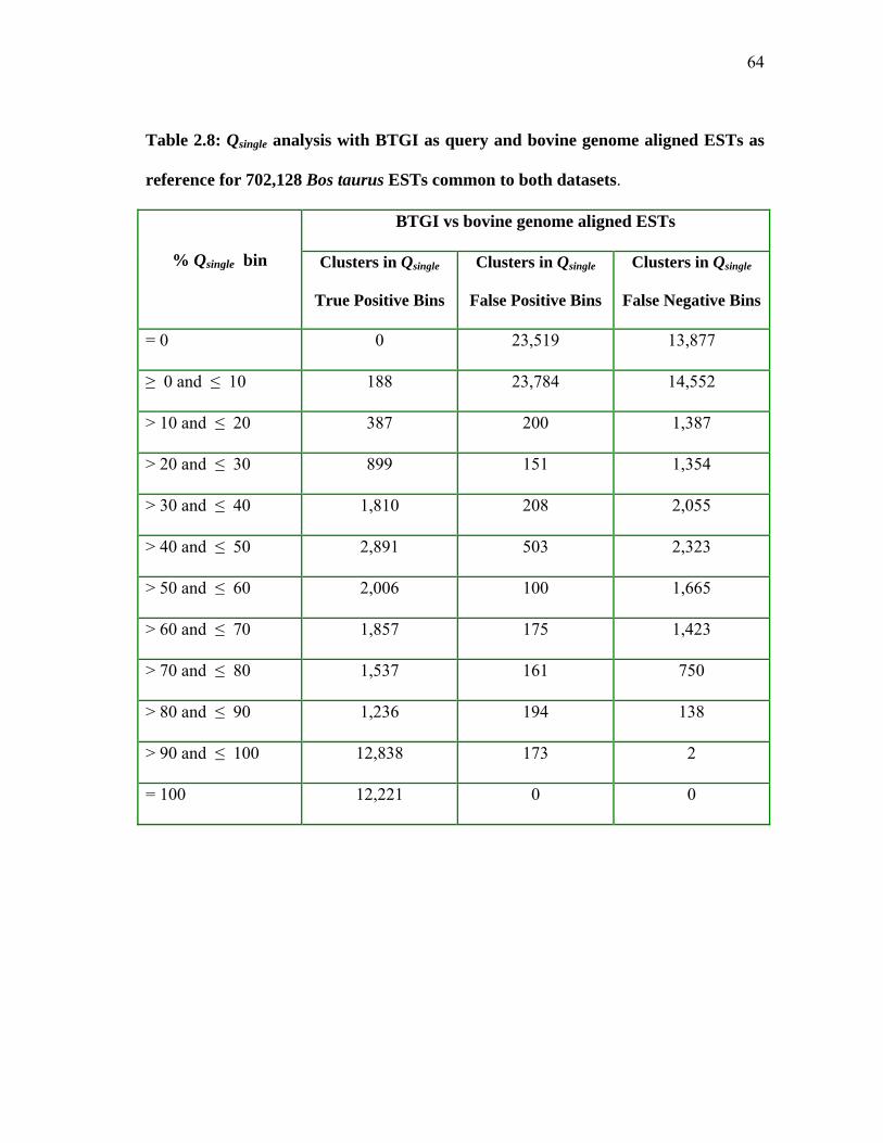
64
Table 2.8: Qsingle analysis with BTGI as query and bovine genome aligned ESTs as
reference for 702,128 Bos taurus ESTs common to both datasets.
% Qsingle bin
BTGI vs bovine genome aligned ESTs
Clusters in Qsingle
True Positive Bins
Clusters in Qsingle
False Positive Bins
Clusters in Qsingle
False Negative Bins
= 0 0 23,519 13,877
≥ 0 and ≤ 10 188 23,784 14,552
> 10 and ≤ 20 387 200 1,387
> 20 and ≤ 30 899 151 1,354
> 30 and ≤ 40 1,810 208 2,055
> 40 and ≤ 50 2,891 503 2,323
> 50 and ≤ 60 2,006 100 1,665
> 60 and ≤ 70 1,857 175 1,423
> 70 and ≤ 80 1,537 161 750
> 80 and ≤ 90 1,236 194 138
> 90 and ≤ 100 12,838 173 2
= 100 12,221 0 0
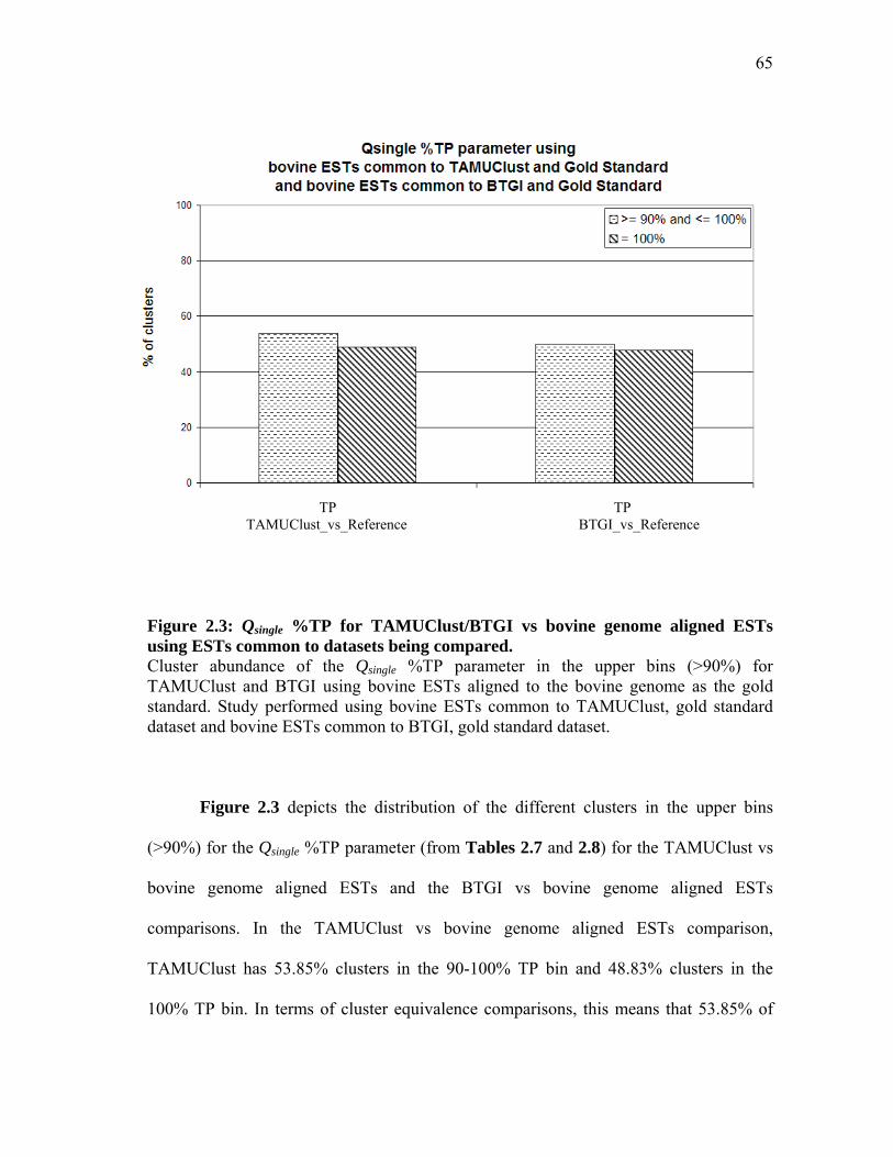
65
TP TP TAMUClust_vs_Reference BTGI_vs_Reference
Figure 2.3: Qsingle %TP for TAMUClust/BTGI vs bovine genome aligned ESTs using ESTs common to datasets being compared. Cluster abundance of the Qsingle %TP parameter in the upper bins (>90%) for TAMUClust and BTGI using bovine ESTs aligned to the bovine genome as the gold standard. Study performed using bovine ESTs common to TAMUClust, gold standard dataset and bovine ESTs common to BTGI, gold standard dataset.
Figure 2.3 depicts the distribution of the different clusters in the upper bins
(>90%) for the Qsingle %TP parameter (from Tables 2.7 and 2.8) for the TAMUClust vs
bovine genome aligned ESTs and the BTGI vs bovine genome aligned ESTs
comparisons. In the TAMUClust vs bovine genome aligned ESTs comparison,
TAMUClust has 53.85% clusters in the 90-100% TP bin and 48.83% clusters in the
100% TP bin. In terms of cluster equivalence comparisons, this means that 53.85% of
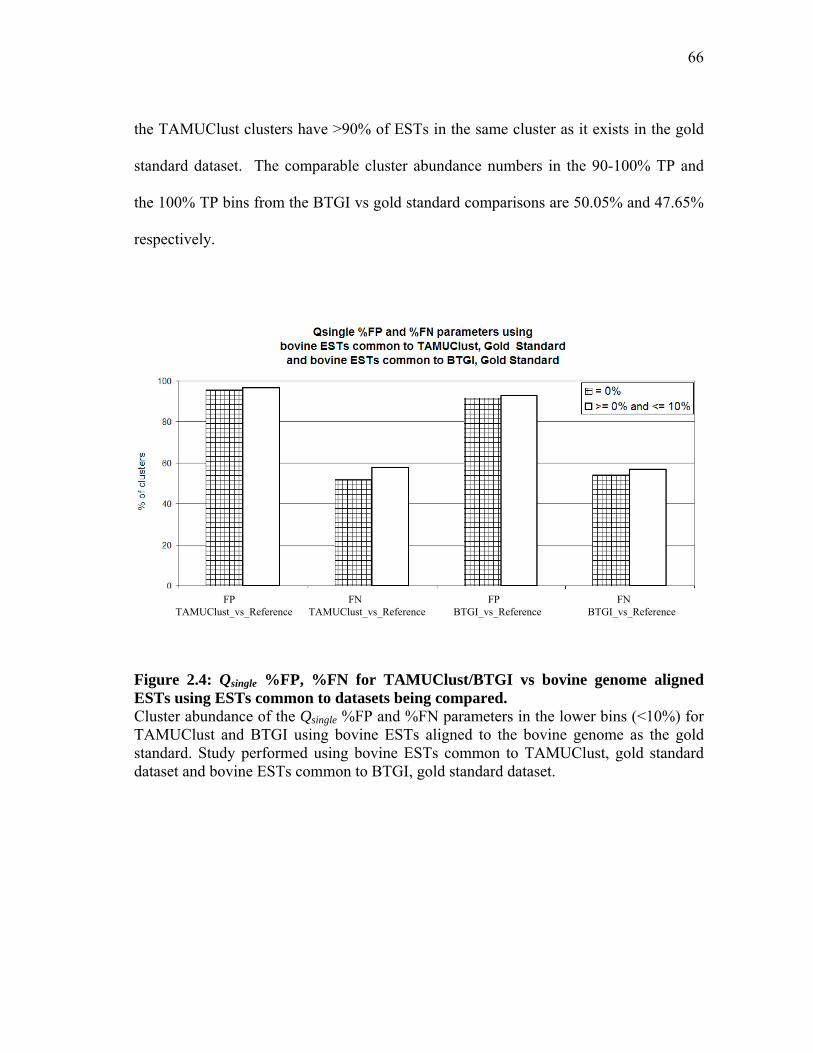
66
the TAMUClust clusters have >90% of ESTs in the same cluster as it exists in the gold
standard dataset. The comparable cluster abundance numbers in the 90-100% TP and
the 100% TP bins from the BTGI vs gold standard comparisons are 50.05% and 47.65%
respectively.
Figure 2.4: Qsingle %FP, %FN for TAMUClust/BTGI vs bovine genome aligned ESTs using ESTs common to datasets being compared. Cluster abundance of the Qsingle %FP and %FN parameters in the lower bins (<10%) for TAMUClust and BTGI using bovine ESTs aligned to the bovine genome as the gold standard. Study performed using bovine ESTs common to TAMUClust, gold standard dataset and bovine ESTs common to BTGI, gold standard dataset.
FP TAMUClust_vs_Reference
FP BTGI_vs_Reference
FN TAMUClust_vs_Reference
FN BTGI_vs_Reference
67
Figure 2.4 depicts the distribution of the different clusters in the lower bins
(<10%) for the Qsingle %FP and %FN parameters for the TAMUClust vs bovine genome
aligned ESTs and the BTGI vs bovine genome aligned ESTs comparisons. The Qsingle
%FP metric for the TAMUClust vs bovine genome aligned ESTs comparison reveals
that TAMUClust has 96.52% clusters in the 0-10% FP bin. This indicates that <10% of
the ESTs in ~97% of the TAMUClust clusters have been grouped with unrelated
members when compared with the corresponding gold standard clusters. The Qsingle %FN
metric for the TAMUClust vs bovine genome aligned ESTs comparison reveals that
TAMUClust has 57.69% clusters in the 0-10% FN bin. This metric indicates that <10%
of the relatives (cluster members) for a particular EST are missing in ~58% of the
TAMUClust clusters when compared with the corresponding gold standard clusters. The
comparable cluster abundance numbers in the 0-10% FP and the 0-10% FN bins from
the BTGI vs bovine genome aligned ESTs comparison are 92.73% and 56.73%
respectively.

68
One also needs to take into account the fact that the dataset in the BTGI-gold
standard analysis is ~3.3 folds larger compared to the dataset in the TAMUClust-gold
standard analysis. The major reason for the ~3.3 folds larger dataset is due to the large
difference in the number of ESTs used to generate the clusters. 308, 132 Bos taurus
ESTs were downloaded from dbEST in March 2005 to generate the TAMUClust EST
clusters, whereas 955, 233 ESTs were present in the BTGI release of March 2007. This
led us to ask the question “Does this difference in datasets being compared affect the
cluster equivalence comparison analysis”. To address this, the above Qsingle analyses
were repeated by using only those ESTs which are common to all 3 datasets. 198,438
bovine ESTs common to all three datasets were identified in the one to one comparisons
of TAMUClust vs bovine genome aligned ESTs and BTGI vs bovine genome aligned
ESTs using bovine ESTs common to all datasets. Qsingle analyses were performed for the
TAMUClust vs bovine genome aligned ESTs and BTGI vs bovine genome aligned
ESTs. The distributions of the Qsingle indices in the different bins and the number of ESTs
in each of the Qsingle %TP, Qsingle %FP and Qsingle %FN bins are detailed in Table 2.9.
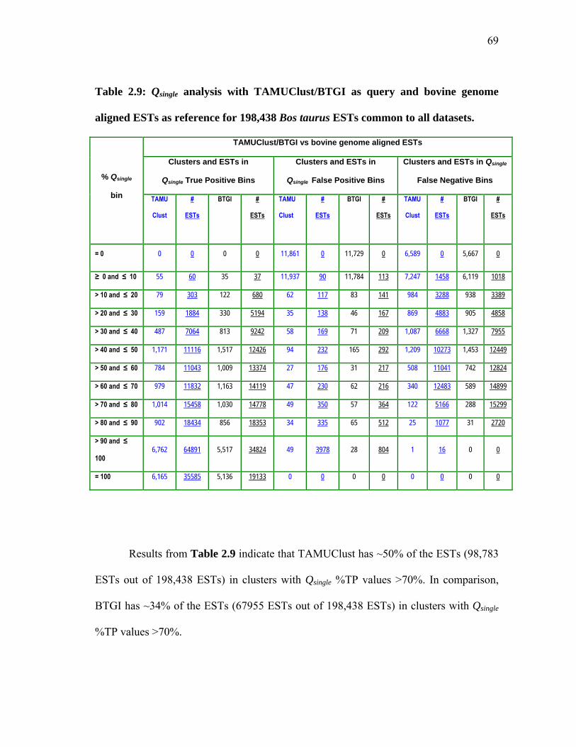
69
Table 2.9: Qsingle analysis with TAMUClust/BTGI as query and bovine genome
aligned ESTs as reference for 198,438 Bos taurus ESTs common to all datasets.
% Qsingle
bin
TAMUClust/BTGI vs bovine genome aligned ESTs
Clusters and ESTs in
Qsingle True Positive Bins
Clusters and ESTs in
Qsingle False Positive Bins
Clusters and ESTs in Qsingle
False Negative Bins
TAMU
Clust
#
ESTs
BTGI #
ESTs
TAMU
Clust
#
ESTs
BTGI #
ESTs
TAMU
Clust
#
ESTs
BTGI #
ESTs
= 0 0 0 0 0 11,861 0 11,729 0 6,589 0 5,667 0
≥ 0 and ≤ 10 55 60 35 37 11,937 90 11,784 113 7,247 1458 6,119 1018
> 10 and ≤ 20 79 303 122 680 62 117 83 141 984 3288 938 3389
> 20 and ≤ 30 159 1884 330 5194 35 138 46 167 869 4883 905 4858
> 30 and ≤ 40 487 7064 813 9242 58 169 71 209 1,087 6668 1,327 7955
> 40 and ≤ 50 1,171 11116 1,517 12426 94 232 165 292 1,209 10273 1,453 12449
> 50 and ≤ 60 784 11043 1,009 13374 27 176 31 217 508 11041 742 12824
> 60 and ≤ 70 979 11832 1,163 14119 47 230 62 216 340 12483 589 14899
> 70 and ≤ 80 1,014 15458 1,030 14778 49 350 57 364 122 5166 288 15299
> 80 and ≤ 90 902 18434 856 18353 34 335 65 512 25 1077 31 2720
> 90 and ≤
100 6,762 64891 5,517 34824 49 3978 28 804 1 16 0 0
= 100 6,165 35585 5,136 19133 0 0 0 0 0 0 0 0
Results from Table 2.9 indicate that TAMUClust has ~50% of the ESTs (98,783
ESTs out of 198,438 ESTs) in clusters with Qsingle %TP values >70%. In comparison,
BTGI has ~34% of the ESTs (67955 ESTs out of 198,438 ESTs) in clusters with Qsingle
%TP values >70%.
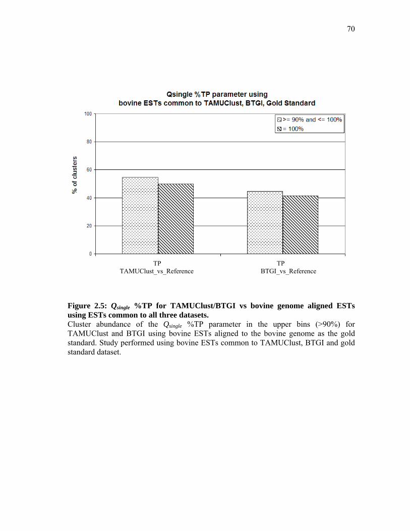
70
TP TP TAMUClust_vs_Reference BTGI_vs_Reference
Figure 2.5: Qsingle %TP for TAMUClust/BTGI vs bovine genome aligned ESTs using ESTs common to all three datasets. Cluster abundance of the Qsingle %TP parameter in the upper bins (>90%) for TAMUClust and BTGI using bovine ESTs aligned to the bovine genome as the gold standard. Study performed using bovine ESTs common to TAMUClust, BTGI and gold standard dataset.

71
Figure 2.5 depicts the distribution of the different clusters in the upper bins
(>90%) for the Qsingle %TP parameter (from Table 2.9) for the TAMUClust vs bovine
genome aligned ESTs and the BTGI vs bovine genome aligned ESTs comparisons using
ESTs common to all datasets. In the TAMUClust vs bovine genome aligned ESTs
comparison, TAMUClust has 54.57% clusters in the 90-100% TP bin and 49.75%
clusters in the 100% TP bin. The comparable cluster abundance numbers in the 90-100%
true-positives and the 100% true-positives bins from the BTGI vs bovine genome
aligned ESTs comparisons are 44.52% and 41.45% respectively.
Figure 2.6: Qsingle %FP, %FN for TAMUClust/BTGI vs bovine genome aligned ESTs using ESTs common to all three datasets. Cluster abundance of the Qsingle %FP and %FN parameters in the lower bins (<10%) for TAMUClust and BTGI using bovine ESTs aligned to the bovine genome as the gold standard. Study performed using bovine ESTs common to TAMUClust, BTGI and gold standard dataset.
FP TAMUClust_vs_Reference
FP BTGI_vs_Reference
FN TAMUClust_vs_Reference
FN BTGI_vs_Reference
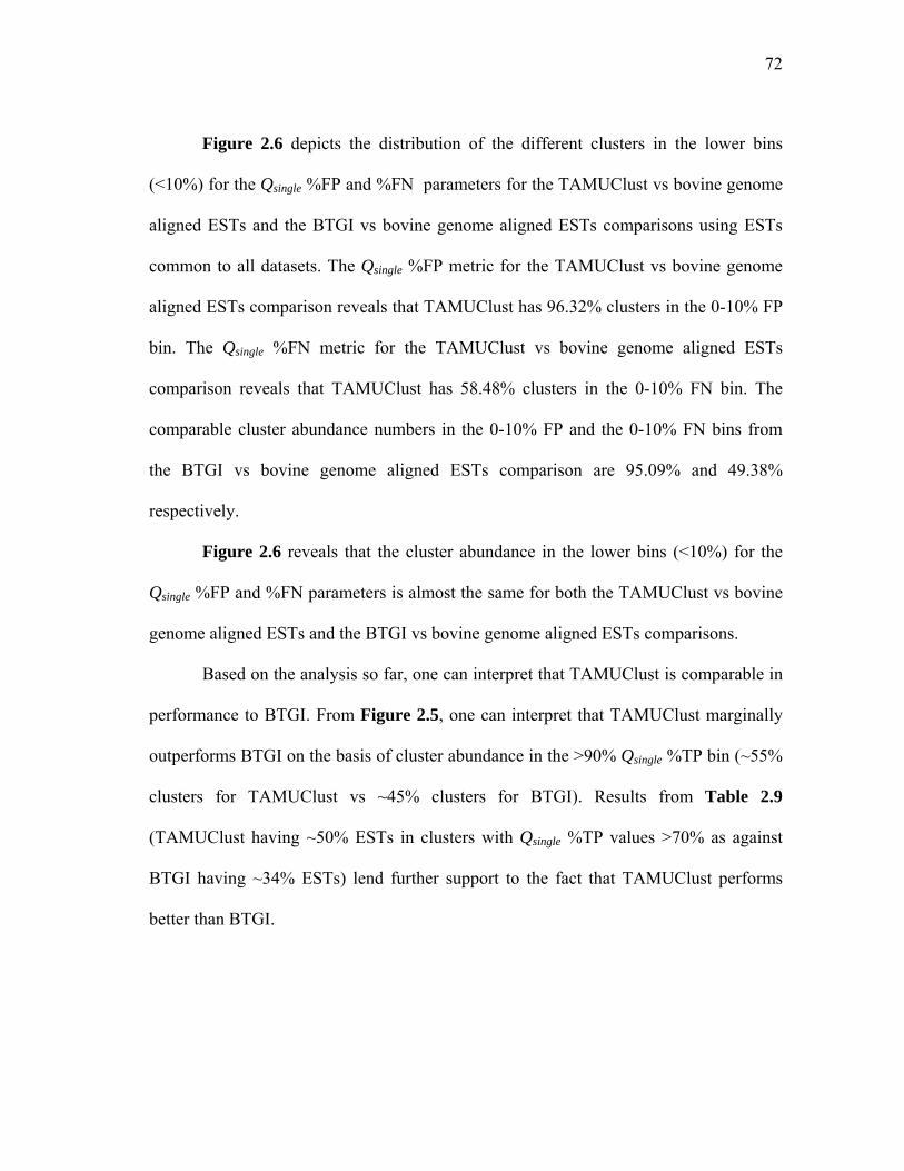
72
Figure 2.6 depicts the distribution of the different clusters in the lower bins
(<10%) for the Qsingle %FP and %FN parameters for the TAMUClust vs bovine genome
aligned ESTs and the BTGI vs bovine genome aligned ESTs comparisons using ESTs
common to all datasets. The Qsingle %FP metric for the TAMUClust vs bovine genome
aligned ESTs comparison reveals that TAMUClust has 96.32% clusters in the 0-10% FP
bin. The Qsingle %FN metric for the TAMUClust vs bovine genome aligned ESTs
comparison reveals that TAMUClust has 58.48% clusters in the 0-10% FN bin. The
comparable cluster abundance numbers in the 0-10% FP and the 0-10% FN bins from
the BTGI vs bovine genome aligned ESTs comparison are 95.09% and 49.38%
respectively.
Figure 2.6 reveals that the cluster abundance in the lower bins (<10%) for the
Qsingle %FP and %FN parameters is almost the same for both the TAMUClust vs bovine
genome aligned ESTs and the BTGI vs bovine genome aligned ESTs comparisons.
Based on the analysis so far, one can interpret that TAMUClust is comparable in
performance to BTGI. From Figure 2.5, one can interpret that TAMUClust marginally
outperforms BTGI on the basis of cluster abundance in the >90% Qsingle %TP bin (~55%
clusters for TAMUClust vs ~45% clusters for BTGI). Results from Table 2.9
(TAMUClust having ~50% ESTs in clusters with Qsingle %TP values >70% as against
BTGI having ~34% ESTs) lend further support to the fact that TAMUClust performs
better than BTGI.
73
Need for ‘singleton minus’ analyses
TAMUClust uses a protein framework to cluster and assemble ESTs. FASTX is
used to compare the ESTs to the vertebrate protein clusters and identify the most closely
related vertebrate protein family for a given EST. For ESTs within each protein family,
the Megablast [114] tool of the TGICL [136] package groups ESTs into clusters by
including ESTs that are at least 95% identical over at least 40 nucleotides and having an
overhang of less than 30 nucleotides. The CAP3 [137] tool assembles the clustered ESTs
into Contigs/Singletons. In this process, TAMUClust also includes singletons in the gene
indices (consensus sequences) it generates where these singletons have a significant
sequence similarity to a homologous protein. BTGI performs a nucleotide-nucleotide
comparison to cluster and assemble ESTs, and discards ESTs that do not match the
clustering criteria. As a result, the gene indices generated by BTGI are devoid of
singletons.

74
‘Singleton minus’ Qsingle analyses were performed by excluding singletons from
the TAMUClust dataset and then comparing TAMUClust/BTGI clusters with the gold
standard (bovine genome aligned ESTs).
Singleton minus analysis I
In the one to one comparisons of TAMUClust vs bovine genome aligned ESTs
and BTGI vs bovine genome aligned ESTs using bovine ESTs common to the datasets
being compared, TAMUClust singletons were excluded and ESTs common to
TAMUClust and the gold standard were identified. This resulted in 198,525 ESTs
common to both datasets.
This TAMUClust versus gold standard dataset Qsingle analysis (Table 2.10) was
compared to the BTGI versus gold standard dataset Qsingle analysis (Table 2.8) using
ESTs common to BTGI and gold standard (702,128 ESTs).
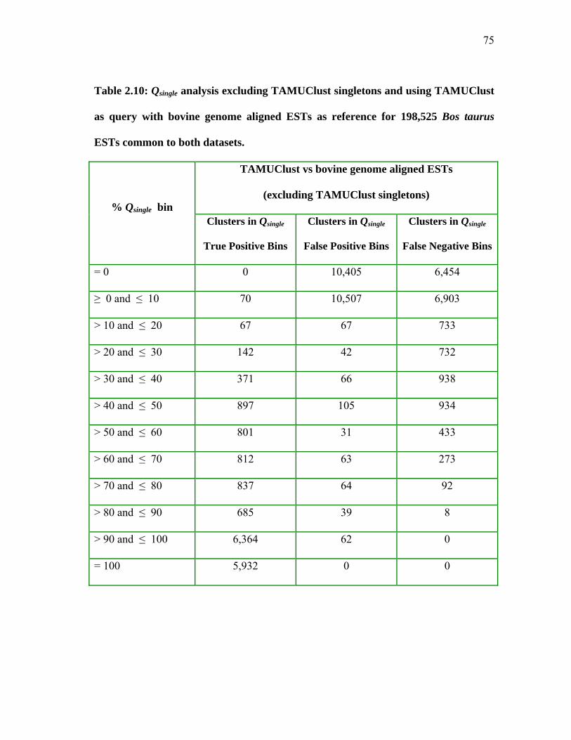
75
Table 2.10: Qsingle analysis excluding TAMUClust singletons and using TAMUClust
as query with bovine genome aligned ESTs as reference for 198,525 Bos taurus
ESTs common to both datasets.
% Qsingle bin
TAMUClust vs bovine genome aligned ESTs
(excluding TAMUClust singletons)
Clusters in Qsingle
True Positive Bins
Clusters in Qsingle
False Positive Bins
Clusters in Qsingle
False Negative Bins
= 0 0 10,405 6,454
≥ 0 and ≤ 10 70 10,507 6,903
> 10 and ≤ 20 67 67 733
> 20 and ≤ 30 142 42 732
> 30 and ≤ 40 371 66 938
> 40 and ≤ 50 897 105 934
> 50 and ≤ 60 801 31 433
> 60 and ≤ 70 812 63 273
> 70 and ≤ 80 837 64 92
> 80 and ≤ 90 685 39 8
> 90 and ≤ 100 6,364 62 0
= 100 5,932 0 0
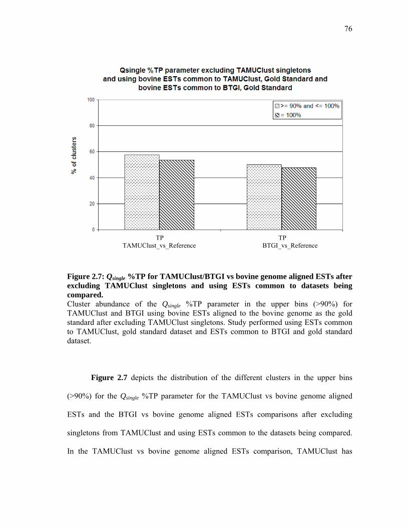
76
TP TP TAMUClust_vs_Reference BTGI_vs_Reference
Figure 2.7: Qsingle %TP for TAMUClust/BTGI vs bovine genome aligned ESTs after excluding TAMUClust singletons and using ESTs common to datasets being compared. Cluster abundance of the Qsingle %TP parameter in the upper bins (>90%) for TAMUClust and BTGI using bovine ESTs aligned to the bovine genome as the gold standard after excluding TAMUClust singletons. Study performed using ESTs common to TAMUClust, gold standard dataset and ESTs common to BTGI and gold standard dataset.
Figure 2.7 depicts the distribution of the different clusters in the upper bins
(>90%) for the Qsingle %TP parameter for the TAMUClust vs bovine genome aligned
ESTs and the BTGI vs bovine genome aligned ESTs comparisons after excluding
singletons from TAMUClust and using ESTs common to the datasets being compared.
In the TAMUClust vs bovine genome aligned ESTs comparison, TAMUClust has
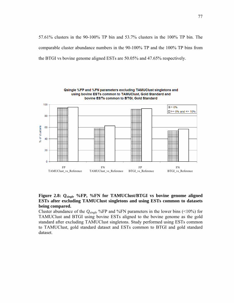
77
57.61% clusters in the 90-100% TP bin and 53.7% clusters in the 100% TP bin. The
comparable cluster abundance numbers in the 90-100% TP and the 100% TP bins from
the BTGI vs bovine genome aligned ESTs are 50.05% and 47.65% respectively.
Figure 2.8: Qsingle %FP, %FN for TAMUClust/BTGI vs bovine genome aligned ESTs after excluding TAMUClust singletons and using ESTs common to datasets being compared. Cluster abundance of the Qsingle %FP and %FN parameters in the lower bins (<10%) for TAMUClust and BTGI using bovine ESTs aligned to the bovine genome as the gold standard after excluding TAMUClust singletons. Study performed using ESTs common to TAMUClust, gold standard dataset and ESTs common to BTGI and gold standard dataset.
FP TAMUClust_vs_Reference
FP BTGI_vs_Reference
FN TAMUClust_vs_Reference
FN BTGI_vs_Reference

78
Figure 2.8 depicts the distribution of the different clusters in the lower bins
(<10%) for the Qsingle %FP and %FN parameters for the TAMUClust vs bovine genome
aligned ESTs and the BTGI vs bovine genome aligned ESTs comparisons after
excluding TAMUClust singletons and using ESTs common to the datasets being
compared. The Qsingle %FP metric for the TAMUClust vs bovine genome aligned ESTs
comparison reveals that TAMUClust has 95.12% clusters in the 0-10% FP bin. The
Qsingle %FN metric for the TAMUClust vs bovine genome aligned ESTs comparison
reveals that TAMUClust has 62.49% clusters in the 0-10% FN bin. The comparable
cluster abundance numbers in the 0-10% FP and the 0-10% FN bins from the BTGI vs
bovine genome aligned ESTs comparison are 92.73% and 56.73% respectively.
Interpretation of results will be difficult when there is a large difference in the
size of datasets being compared. The ‘Singleton minus analysis I’ described above has a
~3.5 fold larger dataset in the BTGI-gold standard analysis compared to TAMUClust-
gold standard dataset. As mentioned before, the ~3.5 fold larger dataset is due to the
large difference in the number of ESTs used in the starting material, which arose because
of the fact that ESTs for TAMUClust were obtained from dbEST in March 2005
whereas the BTGI build was obtained in March 2007.
Singleton minus analysis II
This analysis was performed where the Qsingle indices were obtained by using
only those ESTs which were common to all 3 datasets after excluding TAMUClust
singletons. 192,920 bovine ESTs common to all three datasets were identified after
excluding TAMUClust singletons. Table 2.11 compares the number of clusters and the
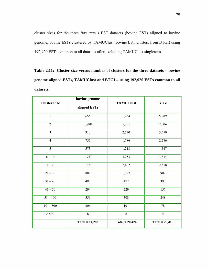
79
cluster sizes for the three Bos taurus EST datasets (bovine ESTs aligned to bovine
genome, bovine ESTs clustered by TAMUClust, bovine EST clusters from BTGI) using
192,920 ESTs common to all datasets after excluding TAMUClust singletons.
Table 2.11: Cluster size versus number of clusters for the three datasets – bovine
genome aligned ESTs, TAMUClust and BTGI – using 192,920 ESTs common to all
datasets.
Cluster Size bovine genome
aligned ESTs TAMUClust BTGI
1 655 1,254 5,989
2 1,788 5,791 7,904
3 910 2,570 3,550
4 752 1,786 2,286
5 573 1,218 1,547
6 – 10 1,957 3,253 3,834
11 – 20 1,871 2,402 2,518
21 – 30 887 1,027 907
31 – 40 488 477 393
41 – 50 294 229 157
51 – 100 559 308 248
101 - 500 206 101 78
> 500 8 8 4
Total = 14,283 Total = 20,424 Total = 29,415
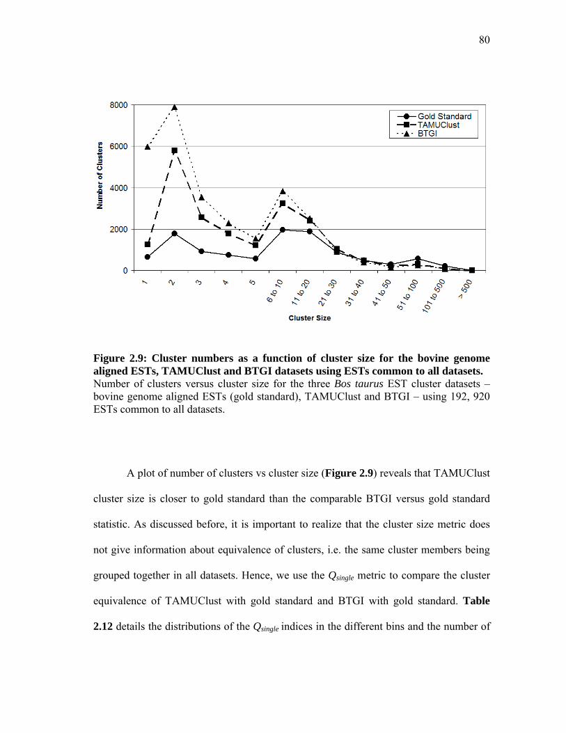
80
Figure 2.9: Cluster numbers as a function of cluster size for the bovine genome aligned ESTs, TAMUClust and BTGI datasets using ESTs common to all datasets. Number of clusters versus cluster size for the three Bos taurus EST cluster datasets – bovine genome aligned ESTs (gold standard), TAMUClust and BTGI – using 192, 920 ESTs common to all datasets.
A plot of number of clusters vs cluster size (Figure 2.9) reveals that TAMUClust
cluster size is closer to gold standard than the comparable BTGI versus gold standard
statistic. As discussed before, it is important to realize that the cluster size metric does
not give information about equivalence of clusters, i.e. the same cluster members being
grouped together in all datasets. Hence, we use the Qsingle metric to compare the cluster
equivalence of TAMUClust with gold standard and BTGI with gold standard. Table
2.12 details the distributions of the Qsingle indices in the different bins and the number of

81
ESTs in each of the Qsingle %TP, Qsingle %FP and Qsingle %FN bins for the TAMUClust vs
gold standard and the BTGI vs gold standard comparisons.
Table 2.12: Qsingle analysis excluding TAMUClust singletons and using
TAMUClust/BTGI as query and bovine genome aligned ESTs as reference for
192,920 Bos taurus ESTs common to all datasets.
% Qsingle
bin
TAMUClust/BTGI vs bovine genome aligned ESTs
Clusters and ESTs in
Qsingle True Positive Bins
Clusters and ESTs in
Qsingle False Positive Bins
Clusters and ESTs in
Qsingle False Negative Bins
TAMU
Clust
#
ESTs
BTGI #
ESTs
TAMU
Clust
#
ESTs
BTGI #
ESTs
TAMU
Clust
#
ESTs
BTGI #
ESTs
= 0 0 0 0 0 10400 0 10444 0 6407 0 4805 0
≥ 0 and ≤ 10 54 59 26 29 10476 90 10493 109 6843 1220 5236 995
> 10 and ≤ 20 63 276 86 601 60 115 65 117 742 3012 849 3249
> 20 and ≤ 30 128 1679 281 4880 35 138 38 152 729 4442 850 4777
> 30 and ≤ 40 368 6573 722 8372 57 161 54 179 926 6713 1201 7264
> 40 and ≤ 50 882 10241 1325 12340 101 241 116 243 917 9164 1307 12063
> 50 and ≤ 60 780 10569 981 13139 28 182 30 213 416 10296 684 12812
> 60 and ≤ 70 786 11420 1013 13326 50 242 45 170 278 11893 550 13833
> 70 and ≤ 80 829 14242 962 14511 56 384 45 316 88 4538 242 14379
> 80 and ≤ 90 687 16745 769 17387 36 359 38 350 9 933 29 2552
> 90 and ≤
100 6,371 68845 4783 36051 49 3978 24 589 0 0 0 0
= 100 5,952 44263 4413 20151 0 0 0 0 0 0 0 0
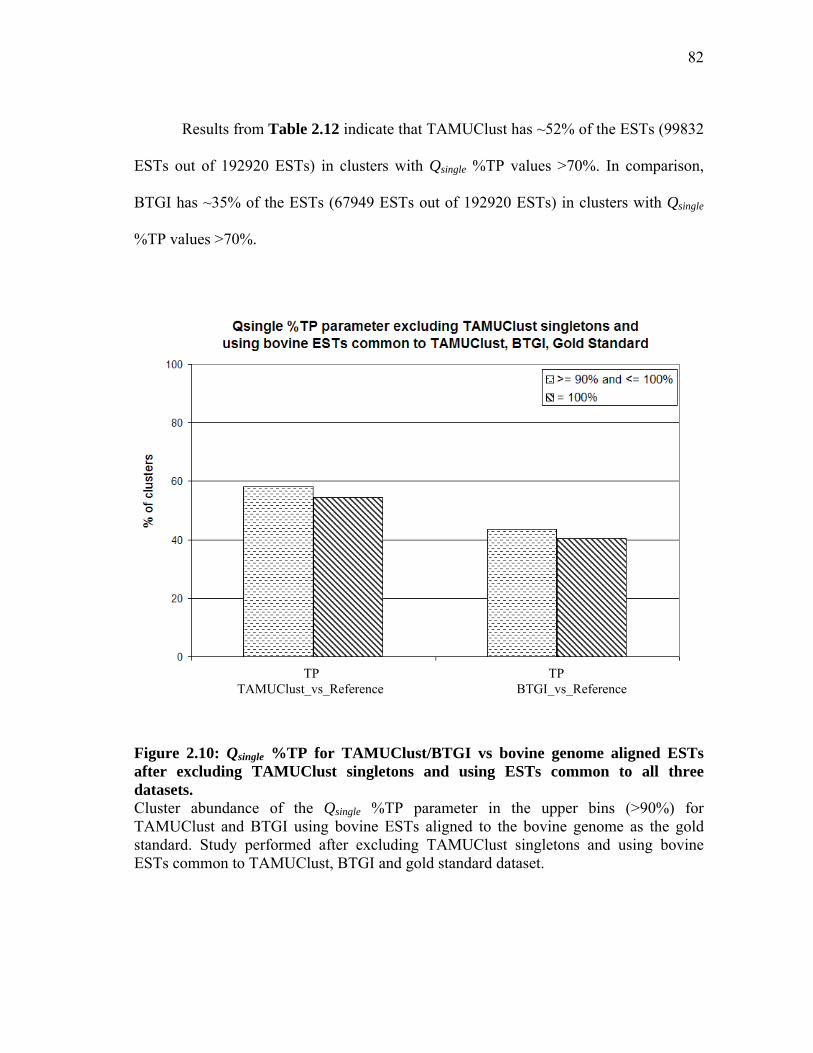
82
Results from Table 2.12 indicate that TAMUClust has ~52% of the ESTs (99832
ESTs out of 192920 ESTs) in clusters with Qsingle %TP values >70%. In comparison,
BTGI has ~35% of the ESTs (67949 ESTs out of 192920 ESTs) in clusters with Qsingle
%TP values >70%.
TP TP TAMUClust_vs_Reference BTGI_vs_Reference
Figure 2.10: Qsingle %TP for TAMUClust/BTGI vs bovine genome aligned ESTs after excluding TAMUClust singletons and using ESTs common to all three datasets. Cluster abundance of the Qsingle %TP parameter in the upper bins (>90%) for TAMUClust and BTGI using bovine ESTs aligned to the bovine genome as the gold standard. Study performed after excluding TAMUClust singletons and using bovine ESTs common to TAMUClust, BTGI and gold standard dataset.

83
Figure 2.10 depicts the distribution of clusters in the 90-100% TP bin and the
100% TP bin using the Qsingle parameter for the TAMUClust vs gold standard and the
BTGI vs gold standard comparisons after excluding TAMUClust singletons and using
ESTs common to all datasets. Figure 2.11 depicts the distribution of the different
clusters in the lower bins (<10%) for the Qsingle %FP and %FN parameters for the
TAMUClust vs gold standard and the BTGI vs gold standard comparisons after
excluding TAMUClust singletons and using ESTs common to all datasets.
FN
TAMUClust_vs_Reference FP BTGI_vs_Reference
FP TAMUClust_vs_Reference
FN BTGI_vs_Reference
Figure 2.11: Qsingle %FP, %FN for TAMUClust/BTGI vs bovine genome aligned ESTs after excluding TAMUClust singletons and using ESTs common to all three datasets. Cluster abundance of the Qsingle %FP and %FN parameters in the lower bins (<10%) for TAMUClust and BTGI using bovine ESTs aligned to the bovine genome as the gold standard. Study performed after excluding TAMUClust singletons and using bovine ESTs common to TAMUClust, BTGI and gold standard dataset.

84
Findings from the Qsingle %FP and %FN indices indicate that TAMUClust and
BTGI perform very similarly. Hence, one can compare the cluster abundance of the
>90% Qsingle percentage true-positives parameter for TAMUClust and BTGI using
bovine genome aligned ESTs as the gold standard to determine which clustering method
performs better.
TAMUClust has 58.19% clusters in the 90-100% true-positives bin compared to
43.69% for BTGI. Comparisons of the 100% true-positives bins reflect a value of
54.37% for TAMUClust and 40.31% for BTGI. In other words, when compared to
BTGI, TAMUClust has ~14-15% additional clusters that have the very same members as
is seen in the gold standard dataset.
The findings from Figure 2.10 taken in conjunction with the findings from
Figure 2.7 and Table 2.12 (TAMUClust having ~52% ESTs in clusters with Qsingle %TP
values >70% as against BTGI having ~35% ESTs) as discussed above illustrate that
TAMUClust performs better than BTGI; removal of singletons from the analysis further
improves the performance of TAMUClust compared to BTGI.
85
Summary of findings from the Qsingle analyses in the Gold standard comparisons
This study was performed to ask the question “Is TAMUClust comparable in
performance to TIGR Gene Indices (TGI)”. Findings from the Qsingle analyses from the
Gold standard comparisons as discussed above suggest that TAMUClust compares well
to TGI and marginally outperforms it.
Comparison with predicted gene models
Megablast analysis I
The Qsingle metric from singleton minus analyses (I and II) using the gold
standard dataset indicates that TAMUClust performs marginally better than BTGI. This
led us to ask the question “Does TAMUClust gain anything by including singletons in its
gene indices”. To address this, we used Megablast [114] to align the consensus
sequences of TAMUClust and BTGI to the bovine transcripts in the Bos taurus Ensembl
Release 50 (July 2008) [129]. For this analysis, we used only the longest transcript for
each gene in the Ensembl dataset. The Megablast results were filtered to include only
those alignments which were longer than 100 bases in alignment length and had
sequence identity greater than 95%. Results from the Megablast analysis I are listed in
Table 2.13.

86
Table 2.13: Megablast analysis I - TAMUClust/BTGI EST consensus sequences vs
Ensembl Btau predicted transcripts.
Criteria TAMUClust BTGI
Number of ESTs 308,132 955,233
Date on which ESTs were obtained March 2005 March 2007
Number of EST consensus sequences
46,731
(24, 665 contigs +
22, 066 singletons)
90, 392
Ensembl transcript hits
34,199
(22, 041 contigs +
12, 158 singletons)
51, 425
Unique Ensembl transcript hits 14, 842 15, 451
Common Ensembl transcript hits 14, 144 14, 144
Ensembl Transcripts that align to
TAMUClust consensus sequences but not to any BTGI consensus sequences
698
(57 contigs +
641 singletons)
-
Ensembl Transcripts that align to BTGI
consensus sequences but not to any TAMUClust consensus sequences
- 1, 307
We first determined if there were any Ensembl transcripts that aligned to
TAMUClust consensus sequences but were missed by BTGI consensus sequences; from
these TAMUClust hits, we then identified the TAMUClust singletons. From Table 2.13,

87
we find that there are 698 Ensembl transcripts that are identified by TAMUClust but are
missed by BTGI. Of these 698 Ensembl transcript hits from TAMUClust consensus
sequences, 641 hits are from singletons.
These results from Table 2.13 indicate that TAMUClust stands to gain by
including singletons. Here are some factors that further reinforce this statement:
1. Date difference in the TAMUClust and BTGI builds: ESTs in TAMUClust
were obtained from GenBank in Mar 2005, whereas the ESTs in BTGI are from
Mar 2007. Despite the fact that there is a ~2 year difference in the dates in favor
of BTGI, Megablast analysis reveals that there are 762 Ensembl transcripts
which align to TAMUClust consensus sequences but not to BTGI consensus
sequences using the alignment filtering criteria (≥95% identity and ≥100 in
alignment length). 641 of these 698 hits were from TAMUClust singletons. By
the same criteria, there are 1,307 Ensembl transcripts that align to BTGI
consensus sequences but not to TAMUClust consensus sequences. We believe
that this is largely due to the difference in the dates of obtaining the ESTs to
build the EST clusters. The only way to prove this beyond doubt would be to
take all the ESTs from the BTGI build and pass it through the TAMUClust
pipeline (vertebrate protein family clustering, ESTs vs protein family FASTX
and EST assembly) – something that is beyond the scope of this project keeping
in mind that the aim of this study is to study how well TAMUClust performs
compared to existing EST clustering schemes and not to prove that TAMUClust
can outdo those schemes.
88
2. Differences in the EST clustering methods: TIGR Gene Indices (TGI) starts off
with gene sequences are parsed from the CDS and CDS-join features in GenBank
protein records pertaining to the species in question [96]; additional Expressed
Transcript (ET) sequences are obtained from the TIGR EGAD database. Coding
Sequences (CDSs), Expressed Transcripts (ETs), and Tentative Consensus
Sequences (TCs) from previous build (if available) are used as templates for the
clustering process. Given the fact that TGI uses TCs from previous build and
CDSs, the average length of the “tentative consensus (TC)” sequence from TGI
is bound to be longer compared to de novo EST clustering methods like
TAMUClust where clusters are built without using information from previous
builds and without using CDSs. By including TCs from previous build and
CDSs, TGI has “longer” starting sequences. Despite these differences in the
EST cluster build with TAMUClust and TGI methodologies, 698 TAMUClust
consensus sequences (of which 641 are singletons) align to Ensembl transcripts
that are missed by BTGI.
3. The TAMUClust singletons have statistically significant similarity to a
homologous protein as determined by the coarse protein grouping performed
prior to EST clustering and assembly. Therefore, the TAMUClust singletons are
not trivial and not some artifacts of the EST clustering method.

89
Summary of findings from Megablast analysis I
This study was performed to ask the question “Does TAMUClust gain anything
by including singletons in its gene indices”. Results from the Megablast analysis in
conjunction with the singleton minus analyses lend further support to the fact that
TAMUClust definitely stands to gain by including singletons in the gene indices
(consensus sequences) it generates.
Comparison with predicted gene models
Megablast analysis II
This analysis was designed to determine how many of the predicted transcripts
from the Bos taurus Ensembl Release 50 (July 2008) [129] have a match to a EST
consensus sequence from the TAMUClust and BTGI Bos taurus EST clusters. Megablast
[114] was used to address this question. The query file being the longest bovine
transcript for each gene from the Bos taurus Ensembl Release 50 and the database was a
file containing either TAMUClust or BTGI EST consensus sequences. There were 21,
722 transcripts in the query file. The Megablast results were filtered to include only
those alignments which were longer than 100 bases in alignment length and had
sequence identity greater than 95%. Results from the Megablast analysis II are listed in
Table 2.14.

90
Table 2.14: Megablast analysis II - Ensembl Btau predicted transcripts vs
TAMUClust/BTGI EST consensus sequences.
Criteria Ensembl Transcripts vs
TAMUClust
Ensembl Transcripts
vs BTGI
Number of ESTs 308,132 955,233
Number of EST consensus
sequences
46,731
(24, 665 contigs +
22, 066 singletons)
90, 392
Hits
16, 194
(13, 282 contigs +
2, 912 singletons)
16, 853
Unique hits 14, 815
(12, 143 contigs +
2, 672 singletons)
15, 459
Number of Ensembl predicted
transcripts in both analyses
15, 559
Ensembl transcripts that align
to TAMUClust consensus
sequences but not to any BTGI
consensus sequences
635
(22 contigs +
613 singletons)
-
Ensembl transcripts that align
to BTGI consensus sequences
but not to any TAMUClust
consensus sequences
- 1, 294

91
Results from Table 2.14 indicate that 16194 (out of a total of 21722) predicted
bovine transcripts have a hit to a TAMUClust EST consensus sequence, whereas 16853
predicted bovine transcripts have a hit to a BTGI EST consensus sequence. Of the 16194
predicted transcripts that had a hit to a TAMUClust EST consensus sequence, 2912 were
to singletons. This further reinforces the point that we had made earlier - TAMUClust
does gain by including singletons in the gene indices it generates.
There are 635 predicted transcripts that align to a TAMUClust EST consensus
sequence but do not align to a BTGI EST consensus sequence. Likewise, there are 1294
predicted transcripts that align to a BTGI EST consensus sequence but do not align to a
TAMUClust EST consensus sequence.
Summary of findings from Megablast analysis II
The overall findings from this analysis suggest that the transcript coverage in
TAMUClust and BTGI is more or less same with the TAMUClust dataset reconstructing
some transcripts that are missed by BTGI and the BTGI dataset reconstructing some
transcripts that are missed by TAMUClust.
CONCLUSIONS
Expressed Sequence Tags (ESTs) are single pass sequence reads from randomly
selected cDNA clone. ESTs contain high error rates, and the information encoded is
often fragmented and redundant. Therefore, ESTs need to be clustered into groups likely
to have been derived from the same genes and this process improves the quality of

92
meaningful information that can be derived from ESTs. Chimeric EST clusters arise
when ESTs representing unrelated genes are grouped together and chimerism is the
single largest contributor to EST misassemblies. This can be avoided if ESTs are
initially grouped into clusters based on their matches to proteins, and then subject to
clustering and assembly. TAMUClust is a new clustering method developed in our lab
which clusters ESTs using a protein framework.
Accurate clustering of ESTs derived from the same genes is of utmost
importance as ESTs are used to identify genes in an organism and in the design of
oligonucleotide probes. Any inaccuracies in the EST clustering step would result in
problems associated with improper oligonucleotide design. EST clustering using a
protein framework is very handy in selecting the representative sets for oligonucleotide
design and helps avoid many of the frequently encountered problems in oligo design -
generating oligos with redundant information, and designing oligos based on chimeric
ESTs.
We conducted a pilot study using Bos taurus ESTs in Jan 2004 to compare the
clustering performance of TAMUClust with existing EST clustering methods, Bos
taurus Gene Indices (BTGI) clusters obtained from DGI/TIGR and UniGene from
NCBI. The study was performed by determining cluster equivalence (Qsingle indices) for
the datasets being compared after identifying common ESTs. The results from the pilot
study indicate that the performance of TAMUClust is comparable to that of BTGI and
UniGene. As the clustering methodology of TAMUClust and BTGI is very much similar
93
with reference to the stringency and the level of supervision, we chose to perform further
comparisons of TAMUClust only with BTGI.
In August 2006, the third version of the bovine genome assembly, Btau_3.1, was
released where the genome assembly has a 7.15X coverage [10, 11]. This came in handy
to compare the performance of TAMUClust Bos taurus EST clusters against the Bos
taurus Gene Indices (BTGI) clusters by using bovine ESTs aligned to the bovine
genome assembly as a gold standard. Findings from the gold standard comparisons
reveal that TAMUClust and BTGI are similar in performance.
An ideal result/situation would have been TAMUClust performing as well as the
gold standard; this not being the case means that there is scope for improvement in the
TAMUClust clustering algorithm. However, one needs to keep in mind that while
clustering ESTs aligned to the genome, it is not required to set a minimum overlap
length due to the fact that two or more overlapping ESTs, irrespective of the overlap
length should belong to the same transcript. This is the reason for the false negatives
when TAMUClust/BTGI is compared to the gold standard dataset. The gold standard
dataset did not include predicted transcripts. If the known coordinates of these predicted
transcripts had been used in the gold standard datasets, the number of false negatives
would have reduced significantly.
When TAMUClust singletons are excluded to be on an even keel with BTGI,
results from the Qsingle analyses suggest that TAMUClust performance is improved
compared to BTGI. However, TAMUClust singletons are not clustering artifacts; these
singletons are included in the gene indices because they have a statistically significant

94
match to a homologous protein used in the protein framework to cluster the ESTs.
Findings from a Megablast analysis using predicted transcripts from the Bos taurus
Ensembl Release 50 (July 2008) [129] suggest that TAMUClust stands to gain by
including the singletons in the gene indices. A second Megablast analysis was designed
to determine how many of the predicted transcripts from the Bos taurus Ensembl Release
50 (July 2008) [129] have a match to a EST consensus sequence from the TAMUClust
and BTGI Bos taurus EST clusters. Findings from this analysis suggest that the
transcript coverage in TAMUClust and BTGI is more or less same with the TAMUClust
dataset reconstructing some transcripts that are missed by BTGI and the BTGI dataset
reconstructing some transcripts that are missed by TAMUClust.
EST clustering methods not based on genome alignments need a framework to
cluster and assemble the ESTs. The framework has to ensure that the clustering method
is neither too rigid to generate very short consensus sequences nor too relaxed to
generate long consensus sequences. Also, in the tradeoff between fewer clusters with
longer consensus and larger clusters with short consensus sequences, the EST clustering
schema has to decide on certain criteria like minimum pairwise sequence identity,
overlap length and overhangs to generate the initial clusters to accurately model the
biology behind the sequences being clustered while incorporating splice variants and
avoiding chimeras.
95
Advantages of TAMUClust
Clustering ESTs using a protein framework helps identify distantly related
(rapidly diverging) protein homologs that might be missed out using DNA:DNA
comparisons. The biggest advantage with the TAMUClust method is that the ESTs are
grouped into gene families as a result of the protein framework being used. This comes
in handy to predict function for these ESTs on the basis of their similarity to the proteins
in the protein family. Moreover, the ESTs in a family can be grouped with the proteins,
subject to phylogenetic analysis and prediction of function by analyzing the tree
topology. Function predictions made using a phylogenetic approach are expected to be
more accurate.
Removal of chimeric ESTs
TAMUClust uses a protein framework to cluster and assemble the ESTs. The
protein comparison step introduces a high level of stringency by removing chimeric
ESTs and reduces the formation of chimeras in the EST assembly step, thereby
preventing misassemblies.
Utility with EST projects from next generation sequencing tools
Sequencing projects are becoming much cheaper nowadays thanks to the use of
the massively parallel 454 pyrosequencing technology [138], which is capable of
sequencing 25 million bases in a four-hour period and is about 100 times faster than the
current Sanger sequencing and capillary-based electrophoresis platform [139]. These
next-generation sequencing tools produce large numbers of short DNA reads (80-120
bases) [138], tend to have low error rates (<1%) arising because of homopolymer runs,
96
and these errors tend to be resolved [140-142] when there is sufficient coverage depth to
allow assembly of overlapping reads. However, the short sequence reads make assembly
of overlapping sequences problematic [143].
EST projects are likely to become much cheaper in the very near future [144],
thanks to next-generation sequencing tools that can sequence large numbers of cDNAs
quickly and cheaply. Traditional EST sequencing projects produce sequences of 200–
500 bases, where each sequence is anchored at the 3' or 5' end of the mRNA transcript.
Using next-generation technology, a form of EST sequencing sometimes referred to as
transcriptome sequencing [145] (where each mRNA is sequenced in its entirety in
random fragments and assembled computationally) is becoming a more feasible strategy
[144] compared to traditional EST sequencing. As of date, published reports of 454
pyrosequencing of transcriptomes are restricted to model species where genomic data or
extensive Sanger EST data served as a reference for EST assembly [146-149]. A
transcriptome study in wasp using 454 ESTs [150] accomplished annotation by
comparisons with the honeybee genome, but did not report EST assembly. Two studies
[147, 149] that used the genome or Sanger EST sequences for mapping and annotation
of 454 ESTs could not accomplish de novo assembly of the 454 EST reads due to the
short sequence reads.
The short sequence reads coming from next generation sequencing tools require
shorter overlap criteria to be used in the assembly, and this increases the chance of
chimeric assemblies. Assembling smaller groups is computationally tractable whereas
lack of computational resources can be a problem with huge short read datasets. In this

97
scenario, the TAMUClust clustering method of using a protein framework is going to be
even more beneficial in assembling short reads and reducing formation of chimeric
assemblies.
A brief on the work in Chapter III and Chapter IV
Chapter III discusses the design and implementation of the Livestock Gene
Family Database – this database has function predictions for bovine and porcine ESTs
that were clustered and assembled using the TAMUClust pipeline using Ensembl
vertebrate protein families as a framework. The resulting EST consensus sequences are
assigned the function of the ‘best match’ Ensembl vertebrate protein following FASTX
[15] searches.
Chapter IV discusses the design and implementation of a phylogenetic annotation
pipeline to predict function for the bovine and porcine ESTs.

98
CHAPTER III
COMPUTATIONAL FUNCTION PREDICTIONS OF THE Bos taurus AND Sus
scrofa TRANSCRIPTOMES USING THE BEST MATCH APPROACH
SYNOPSIS
Bos taurus (cattle) and Sus scrofa (pig) are important livestock species that
occupy a large proportion of the meat industry and also serve as good candidate animal
models for biomedical research due to parallels with humans. The genome sequences for
these species are in far from being complete and hence, Expressed Sequence Tag (EST)
datasets were used to determine what genes are there and what roles they play. Cattle
and pig ESTs were first clustered into gene families using the vertebrate proteomes in
the Ensembl database as a framework, and the resulting EST consensus sequences were
electronically annotated with the function of the ‘best match’ Ensembl vertebrate
protein. These annotations are housed in the ‘Livestock EST Gene Family Database’
(http://genomes.arc.georgetown.edu/cgi-bin/search_livestock_est_gene_family.cgi). The
database currently hosts annotations for 46,731 bovine EST consensus sequences and
39,641 porcine EST consensus sequences. The database has a user-friendly web
interface and can be searched in a number of ways: Cattle/Pig EST GenBank identifiers
(GI or Accession), Gene Ontology Accession to obtain information about the vertebrate
protein family, related EST members and other annotations. These annotations would
guide the livestock community in helping narrow down the gamut of direct experiments
needed to verify function.
99
BACKGROUND
Utility of cattle and pigs in biomedical research
Bos taurus (cattle) and Sus scrofa (pig) are important livestock species that not
only occupy a large proportion of the meat industry, but also serve as candidate animal
models for biomedical research. Bos taurus and Sus scrofa represent evolutionary clades
distinct from the primates and the rodents, and serve as important model organisms for
health research due to parallels with humans [151, 152]. The cattle genome is useful in
comparative genomics for studies that benefit human health [151] in the areas of obesity,
reproductive biology, lactation and infectious diseases. It is also useful in studies of
endocrinology, physiology and reproductive techniques [151]. Similarities between
humans and pigs exist in digestive physiology, renal function, vascular structure, and
respiratory rates [152]. Pigs are also used as model organism in many areas of medical
research including obesity, cardiovascular disease, endocrinology, alcoholism, diabetes,
nephropathy, and organ transplantation [152]. The pig also serves as a possible candidate
animal model for biomedical research addressing regenerative medicine or preclinical
investigations in pharmacology [153]. The importance of cattle and pigs in agriculture
and medicine demands that we have a sound knowledge of the molecular biology of the
species and the functions they encode as represented by their genome sequences and
gene expression data.

100
Connecting sequence to biology – function predictions using EST datasets
Genome research requires developing resources like linkage maps, physical
maps, and bacterial artificial chromosome (BAC) libraries to organize vast amounts of
genetic information that can be easily accessed and characterized [154]. The availability
of a high-quality annotated genome sequence is an invaluable tool for the biologist as it
bridges the gap from the sequence to the biology of the organism [155], where the aim of
high-quality annotation is to identify the key features of the genome – in particular, the
genes and their products. The scientific community is becoming increasingly reliant on
the tools and resources of annotation to derive information for most aspects of biological
research [155].
Most eukaryotic organisms do not have a complete genome sequence available;
instead, what is available is a large collection of expressed sequence tags (ESTs)
obtained by random sequencing of cDNA copies of cell mRNA sequences. ESTs are
short (200 to 500 bases), unedited single-pass sequence reads of cDNA clones, and
provide a high-throughput means to sample an organism’s transcriptome [8, 98] and
identify expressed genes. EST projects provide a wealth of genetic information for a
species as they often shorten the laborious process of gene isolation and also provide the
raw material for expression profiling utilizing microarrays based on the transcript
sequences [154]. One can use EST datasets to identify genes and obtain insights about
the functions they encode by comparing the sequence against other sequences in a
database, identifying a sequence whose similarity is statistically significant, and
transferring the annotation of known (or presumed) function of the database hit to the
101
query sequence. This strategy of annotation transfer helps connect the ESTs to the
‘putative’ functions they encode. A common strategy for detecting homologs and
obtaining function annotations for EST datasets is to search well-annotated proteomes
using BLASTX/FASTX (translated DNA query against a protein database), obtain
information about the homolog with the “best hit” and to transfer the annotations of the
“best hit” match to the EST sequence [104-106].
Describing biological knowledge using structured annotation vocabularies
Extracting relevant biological information about genes and gene products is often
confounded by the lack or incompleteness of annotations. In such a scenario, the
controlled (or structured) vocabularies describing domains of molecular biology
developed by the Gene Ontology (GO) Consortium [156, 157] can be used to describe
gene products in any organism. These ontologies are expert-curated and describe gene
products in terms of their associated biological processes, cellular components and
molecular functions in a species-independent manner. Each term can have one or more
relationships with other terms, reflecting the complexity of the underlying biology.
Formally, the structure and the format [158] of GO is a directed acyclic graph (DAG)
[159] wherein the terms are equivalent to nodes of the graph and the relationships are
equivalent to edges.
As part of a controlled vocabulary, the different terms in GO have precise
definitions and precise relationships to other terms. GO represents the different
vocabulary terms in a hierarchically structured format and the vocabulary terms are
102
linked to each other by "is a" and "part of" relationships, thus ensuring that very general
terms as well as very precise terms are both represented. Doing so results in a set of
parent-child relationships between different terms, where a child (more specialized term)
is a subset of a parent’s (less specialized term) elements. Given this hierarchical nature
of the GO, all child terms inherit the properties of their parents. This feature comes in
handy to profile function at a coarser (parent) level and incorporating the function
annotations at the finer (children) level by navigating the GO hierarchy.
Overview of the work in this chapter
This chapter is a case study that utilizes EST datasets and addresses the issue of
obtaining insights of the function encoded in the Bos taurus and the Sus scrofa
transcriptomes using computational predictions. The pipeline developed adopts a
comparative genomics approach involving database similarity searches of the Bos taurus
and the Sus scrofa EST datasets against well-annotated vertebrate proteomes, and the
transfer of function annotations of the database sequence whose similarity was
statistically significant. The Bos taurus genome is in the final draft assembly (7.1X
coverage) [10, 11]; a 6X coverage of the Sus scrofa has been proposed [12] with the
current assembly (as of Jun 2008) being available with a 3 fold coverage.
Part I of this chapter discusses the design and implementation of the annotation
pipeline of “The Livestock Gene Family Database” consisting of cattle and pig ESTs.
These ESTs are grouped into gene families using the protein families obtained from an
in-house clustering algorithm (described in Chapter II) following the clustering of the
103
different vertebrate proteomes in the Ensembl [9] database. The resulting EST gene
families were electronically annotated using Gene Ontology terms (GO) of the ‘best
match Ensembl vertebrate protein’ following FASTX [15] searches using a BLOSUM62
[160] matrix and a E-value cutoff ≤ 1E-3. Methods described in Chapter II were used to
select EST consensus sequences leading to the design of 70-mer oligonucleotide probes.
These probes were used to profile the expression of the cattle and pig genomes as part of
the Bovine Oligo Microarray Consortium [161] and the Swine Protein-Annotated
Oligonucleotide Microarray [162] projects, respectively. Methods described in this
chapter (‘Best Hit’ approach) were used to annotate the oligos.
Part II of this chapter discusses the findings of a Gene Ontology function
categorization on the cattle and pig transcriptomes performed using the generic GO Slim
[163]. In this analysis, the distribution of the genes in each of the main ontology
categories was examined and the percentages of the unique sequences in each of the
assigned GO terms from the GO Slim were computed. This GO Slim analysis takes into
consideration the directed acyclic graph (DAG) model of the GO schema and in doing
so, it accounts for the fact that all child terms of a particular GO accession inherit the
property of the parent.
MATERIALS AND METHODS
Clustering of cattle and pig ESTs
ESTs were clustered into gene families using the TAMUClust algorithm as
described in Chapter II. This clustering algorithm is a two-step process and uses the

104
vertebrate proteomes in the Ensembl database as a framework to assemble and translate
the ESTs. ESTs were downloaded from dbEST [101] in March 2005 and were subject to
cleaning and trimming as described in Chapter II to obtain 'high quality' ESTs. This
resulted in 308,132 high quality ESTs from Bos taurus and 238,691 high quality ESTs
from Sus scrofa. Ensembl vertebrate proteins were downloaded from the Ensembl site in
April 2005. The different Ensembl vertebrate proteome datasets used were: Homo
sapiens, Mus musculus, Rattus norvegicus, Gallus gallus, Danio rerio, Takifugu rubripes
and Tetraodon nigroviridis.
In the first step of the clustering process, vertebrate proteomes are grouped into
protein families using a combination of single and average linkage clustering. This
resulted in 10,092 clusters of protein families from a total of 219,433 proteins. In the
second step of the clustering process, The Gene Indices Clustering tools or TGICL [136]
was used to cluster and assemble the ESTs using the vertebrate protein families served
as a framework. This resulted in EST consensus sequence (EST gene families) as
described in Chapter II. In this process, 308,132 bovine ESTs were grouped into 46,731
EST consensus sequences (24,665 contigs and 22,066 singletons); and the 238,691
porcine ESTs were grouped into 39,641 EST consensus sequences (20,951 contigs and
18,690 singletons).
The EST contigs/singletons generated follow this naming convention:
'Integer1_CLInteger2ContigInteger3', where Integer1 is the Protein Family ID assigned
by the protein clustering algorithm, CLInteger2 refers to a particular Cluster ID
(assigned by Megablast from the TGICL package) and ContigInteger3 refers to the
105
Contig ID (assigned by CAP3 from the TGICL package) for that cluster. As an example,
for the EST Contig 6144_CL1Contig2, the integer 6144 denotes the Protein Family ID,
CL1 represents the first EST Megablast cluster matching the Protein Family 6144 and
Contig2 represents the second Contig generated by CAP3 assembly of the different
ESTs belonging to ProteinFamily6144_Cluster1. Similarly, the singletons have this
naming convention: 'Integer1_GI' where Integer1 is the Protein Family ID assigned by
the protein clustering algorithm and GI is the GenBank GenInfo Identifier for the
particular EST.
Design of the ‘GBrowse EST Assembly Viewers’
EST clustering results in contigs and singletons. The contig is a consensus
sequence of several ESTs. The contig files for bovine and porcine ESTs generated by
TAMUClust were parsed using Perl to obtain the different EST Contig alignment files.
Each file consists of the EST Contig and the alignment of the constituent ESTs to the
Contig. Further Perl processing was done to extract information underlying in these EST
Contig alignment files to generate gff3 [135] and fasta files required for the design of the
GBrowse [164] interface. The information pertaining to the EST Contig alignments for
the Bos taurus and the Sus scrofa ESTs used in this study are accessible over the web:
• “The Cattle EST Assembly Viewer” is available from
http://genomes.arc.georgetown.edu/cgi-bin/gbrowse/cattle_ests_test/
• The Pig EST Assembly Viewer” is available from
http://genomes.arc.georgetown.edu/cgi-bin/gbrowse/pig_ests/

106
Annotation pipeline for the Livestock EST gene families
The steps outlined below describe the annotation pipeline developed for
annotating the cattle and porcine EST gene families obtained by clustering ESTs using
the TAMUClust clustering pipeline (described in more detail in Chapter II).
1. Determining the “best match” Ensembl vertebrate protein for an EST
Contig/Singleton: The Ensembl vertebrate proteins were filtered for low-
complexity regions using the PSEG [165, 166] tool. The “best match” Ensembl
vertebrate protein for a livestock EST Contig/Singleton was determined within a
single species following a FASTX [15] search against the different Ensembl
vertebrate proteomes using the BLOSUM62 scoring matrix and E-value cutoff
≤10-3. Following the FASTX searches, the “best match” Ensembl vertebrate
protein for an EST Contig/Singleton within a proteome was determined from
amongst the various proteomes using this order of precedence: Homo sapiens,
Mus musculus, Rattus norvegicus, Gallus gallus, Danio rerio, Takifugu rubripes
and Tetraodon nigroviridis. For example, if a livestock EST Contig/Singleton
does not have a match in Homo sapiens, the best match is searched in the next
species using the precedence order mentioned above till a best match in a species
is found. This order of precedence used here is based on the evolutionary
distance relative to bovine/porcine.
2. Determining the “best match” Ensembl vertebrate protein having a Gene
Ontology (GO) Annotation: The Gene Ontology cross-references and other
database (NCBI, UniProt) protein cross-references for the Ensembl vertebrate
107
proteins were obtained from BioMart [167]. Information pertaining to the Gene
Ontologies was obtained from the GO CVS repository at the Gene Ontology
Consortium [156]. The above mentioned pipeline is used to determine the “best
match” Ensembl vertebrate protein for a particular EST Contig/Singleton. If the
“best match” Ensembl vertebrate protein does not have a GO Annotation, then
the best match Ensembl protein (with GO annotation) is determined from the
next species using the order of precedence mentioned above.
Design and implementation of the ‘Livestock EST Gene Family Database’
The electronic annotations for the cattle and pig EST gene families can be
accessed over the web from “The Livestock EST Gene Family Database” available at:
http://genomes.arc.georgetown.edu/cgi-bin/search_livestock_est_gene_family.cgi. The
database web server was setup using a LAMPerl (Linux, Apache, MySQL, Perl CGI)
environment. The Livestock EST Gene Family Database has two underlying components
representing the species-specific webpages:
• the Cattle EST Gene Family Database available at
http://genomes.arc.georgetown.edu/cgi-bin/search_cattle_est_gene_family.cgi
• the Pig EST Gene Family Database available at
http://genomes.arc.georgetown.edu/cgi-bin/search_porcine_est_gene_family.cgi

108
‘GO Slim’ analysis
GO Slim [163] is a list of high level GO terms covering all three GO categories
and the GO Slim terms provide biological meaning at a coarser level of resolution. The
hierarchical classification of GO was utilized to obtain a broader function analysis of GO
mapped annotations. To incorporate and encompass the fine-level (child level) gene
annotations to arbitrary coarser levels (parent) found in the GO Slims, we first
determined recursively all the descendants (parent-child relationships) for a given GO
Slim term. In the next step, the complete descendant information of a given GO Slim
term was used to map all the descendants associated with the GO Slim term to their
respective gene products from the Livestock EST Gene Families. The steps detailed
below outline the pipeline used in the GO Slim analysis of the Livestock EST Gene
Families:
1. The “go-term-db” tables were obtained from the Gene Ontology Archive [168];
these tables contain information on the GO terms and relationships. The “go-
term-db” tables were loaded into a local MySQL database (say DB1). A different
MySQL database (say DB2) housed the information pertaining to the
cattle/porcine EST contigs and singletons mapped to their respective “best
match” Ensembl vertebrate proteins and GO Annotations associated with the
Ensembl protein.
2. A function analysis using Gene Ontology (GO) categories was performed on the
cattle and porcine EST gene families using the GO Slim [163] developed and
maintained by the Gene Ontology Consortium [156]. The generic GO Slim [169]
109
was obtained and was parsed using Perl to obtain a tab-delimited file containing
the GO ID and GO terms. For every term in the GO Slim, Perl-DBI scripts were
used to query the “go-term-db” tables in DB1 and obtain the complete
descendant information.
3. Once the complete descendant information for a particular GO Slim term is
obtained, Perl-DBI scripts were used to query DB2 for each of the descendants
and to obtain the cattle/porcine EST contigs and singletons mapped to it.
RESULTS AND DISCUSSION
The first part of this section describes the utility of the “Livestock EST Gene
Family Database”. The different search tools allow the user to search by any attribute of
a sequence (cattle/pig EST GI or GenBank accession), sequence cluster (cattle/pig EST
Contig or Protein Family ID), and Gene Ontology (GO) accessions. The Livestock EST
Gene Family Database (Figure 3.1) has two underlying components representing the
species-specific webpages:
1. The Cattle EST Gene Family Database (Figure 3.2) available at:
http://genomes.arc.georgetown.edu/cgi-bin/search_cattle_est_gene_family.cgi
2. Pig EST Gene Family Database (Figure 3.3) available at:
http://genomes.arc.georgetown.edu/cgi-bin/search_porcine_est_gene_family.cgi

110
Figure 3.1: Home page of the Livestock EST Gene Family Database. Figure 3.2: Home page of the Cattle EST Gene Family Database.

111
Figure 3.3: Home page of the Pig EST Gene Family Database.
112
The Livestock EST Gene Family Database provides a user-friendly interface for
searching, browsing and retrieval of information. One can search the database in
different ways as detailed below.
Search by cattle/pig GenBank identifiers (GI or Accession)
The search results page for this search would indicate if the EST is part of a EST
Contig or a Singleton, and for EST Contigs, a GBrowse [164] link depicting the
alignment of the different ESTs to the EST Contig is provided. The search results page
also has information regarding the ‘best match Ensembl vertebrate protein’ with/without
GO Annotations for the EST Contig/Singleton, and the GO and the NCBI and UniProt
protein cross-references for the Ensembl protein. The results page also provides
information about other EST contigs and singletons constituting the protein family
associated with the EST searched. Figure 3.4 is a screenshot showing the search results
from the “Livestock EST Gene Family Database” upon searching for the Bos taurus EST
GenBank GI 12123209.

113
Figure 3.4: Search results for the Cattle EST GenBank GI 12123209 from the Livestock EST Gene Family Database.
114
Search by cattle/pig ‘EST Contig or Singleton’
If a user has prior information about a specific EST Contig or Singleton and is
interested in getting further details about the same, one can search the “Livestock EST
Gene Family Database” for the same. The search results would detail the annotations,
database cross-references, protein family details, and in case of EST contigs a GBrowse
[164] link is provided. The EST contigs follow this naming convention:
'Integer1_CLInteger2ContigInteger3', where Integer1 is the Protein Family ID assigned
by the protein clustering algorithm, CLInteger2 refers to a particular Cluster ID
(assigned by Megablast from the TGICL package) and ContigInteger3 refers to the
Contig ID (assigned by CAP3 from the TGICL package) for that cluster. In case of
singletons, the names are of the type 'Integer1_GINumber', where Integer1 is the Protein
Family ID assigned by the protein clustering algorithm, and GI Number is the GenBank
GeneInfo Number for that EST. Figure 3.5 is a screenshot showing the search results
from the “Livestock EST Gene Family Database” upon searching for the Sus scrofa EST
Contig 10_CL4Contig1.
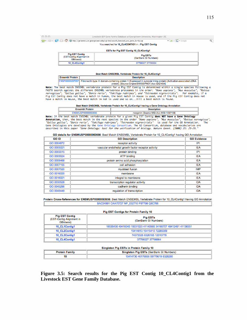
115
Figure 3.5: Search results for the Pig EST Contig 10_CL4Contig1 from the Livestock EST Gene Family Database.
116
Search by ‘Protein Family ID’
Searching by Protein Family ID would detail the different members of the Bos
taurus and Sus scrofa EST gene families, and the different Ensembl vertebrate proteins
belonging to that protein family. Links for the individual annotations for the different
members of the Bos taurus and Sus scrofa EST gene families, and information
pertaining to the different vertebrate proteins constituting the protein family are also
provided. It is to be noted that the 'Protein Family ID' is a number internal to this
database and denotes the ID assigned by the protein clustering algorithm.
The salient feature of the “Protein Family” search is that one can get a listing of
ESTs belonging to the same gene/protein family and represented in two different species
(cattle and pig). This information is particularly useful in situations where a researcher,
say from the pig community, is interested in the putative functions of a specific pig EST
and would like to know the ESTs in cattle which perform a similar function. To obtain
this information, the researcher would first search the “Livestock EST Gene Family
Database” using the pig EST GenBank accession as a query, obtain the putative function
annotations for that pig EST and note the “Protein Family ID” to which the pig EST
belongs. In the second step, the researcher would search the “Livestock EST Gene
Family Database” using the “Protein Family ID” as the query and obtain information
about different cattle and pig ESTs in that protein family. Figure 3.6 is a screenshot of
the search results from the “Livestock EST Gene Family Database” listing the Bos
taurus and Sus scrofa EST gene families, and the different Ensembl vertebrate proteins
upon searching for the Protein Family 15939.

117
Figure 3.6: Search results for Protein Family ID 15939 from the Livestock EST Gene Family Database.

118
Search by ‘Gene Ontology Accession’
This search will find all gene products (EST Contig/Singletons in this case)
directly annotated to the GO accession as well as other gene products transitively
annotated. To elaborate, this search functionality above takes into consideration the
directed acyclic graph (DAG) model and the hierarchical classification of ontologies in
the GO schema where a child (more specialized term) is a subset of a parent’s (less
specialized term) elements. For example, if gene product GP is annotated to GO:X, and
GO:X is beneath GO:Y, then GP is transitively annotated to GO:Y. Therefore, all child
terms of a particular GO accession inherit the properties of the parent. Searching by GO
accession on this database will retrieve its complete descendant information and the
mapping of the different EST contigs/singletons associated with the complete GO
descendant tree starting from that GO Accession. This search feature will come in handy
for users who want to get a complete profile of gene products associated with a
particular GO Accession. As an example, lets say a researcher was interested in finding
cattle and pig EST gene products annotated to the GO accession “GO:0006110 –
regulation of glycolysis”. GO:0006110 has two child terms; GO:0045821 – positive
regulation of glycolysis and GO:0045820 – negative regulation of glycolysis. Given the
hierarchical organization of GO, the child terms GO:0045820 and GO:0045821 inherit
the properties of the parent GO:0006110. A search for GO:0006110 at the “Livestock
EST Gene Family Database” would first identify its complete descendant tree and then
map the different cattle and pig EST gene products to all of the GO accessions in the
descendant tree. Doing it this way, the researcher can get a snapshot of all the cattle and
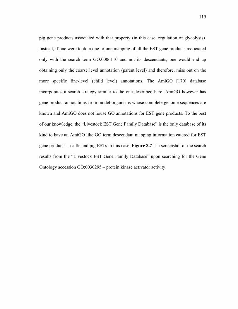
119
pig gene products associated with that property (in this case, regulation of glycolysis).
Instead, if one were to do a one-to-one mapping of all the EST gene products associated
only with the search term GO:0006110 and not its descendants, one would end up
obtaining only the coarse level annotation (parent level) and therefore, miss out on the
more specific fine-level (child level) annotations. The AmiGO [170] database
incorporates a search strategy similar to the one described here. AmiGO however has
gene product annotations from model organisms whose complete genome sequences are
known and AmiGO does not house GO annotations for EST gene products. To the best
of our knowledge, the “Livestock EST Gene Family Database” is the only database of its
kind to have an AmiGO like GO term descendant mapping information catered for EST
gene products – cattle and pig ESTs in this case. Figure 3.7 is a screenshot of the search
results from the “Livestock EST Gene Family Database” upon searching for the Gene
Ontology accession GO:0030295 – protein kinase activator activity.
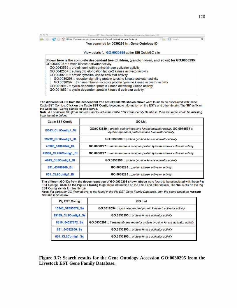
120
Figure 3.7: Search results for the Gene Ontology Accession GO:0030295 from the Livestock EST Gene Family Database.

121
Search by microarray ‘Oligo Locus’ or ‘Oligo ID’
The EST clustering process resulted in a set of Unique Transcripts (UT) which
includes EST Contigs and Singletons. Unique Transcripts overlapping the same
vertebrate Ensembl protein were identified and these "groups of Unique Transcripts" are
in effect "groups of genes". As part of the Bovine Oligo Microarray Consortium [161]
and the Swine Protein-Annotated Oligonucleotide Microarray [162] projects, novel 70-
mer oligonucleotide probes were designed for profiling gene expression of the cattle and
pig genomes with one oligo being designed per gene. The Cattle EST Gene Family
Database has information pertaining to the 16,846 oligonucleotide sequences designed
for the Bovine Oligo Microarray Consortium [161]; the Pig EST Gene Family Database
has information pertaining to the 18,254 oligonucleotide probes designed for the Swine
Protein-Annotated Oligonucleotide Microarray [162] project. On the specific EST Gene
Family webpages (Figure 3.2 and Figure 3.3), searching for the Microarray Oligo
Locus or ID retrieves information about the consensus oligo sequence it represents, the
EST Contig or Singleton associated with the oligo sequence, and the annotations and
other cross-references associated with EST Contig or Singleton. Figure 3.8 is a
screenshot of the search results from the “Cattle EST Gene Family Database” upon
searching for the Bovine Oligo Microarray Consortium (BOMC) Locus 11695. Figure
3.9 is a screenshot of the search results from the “Pig EST Gene Family Database” upon
searching for the Pig MicroArray Oligo ID 10033:7213_CL4Contig1:F.

122
Figure 3.8: Search results for Bovine Oligo Microarray Consortium Locus 11695 from the Cattle EST Gene Family Database.

123
Figure 3.9: Search results for Pig MicroArray Oligo ID 10033:7213_CL4Contig1:F from the Pig EST Gene Family Database.
124
Cattle/Pig ‘EST Assembly Viewers’ in GBrowse
Generic Genome Browser (GBrowse) is a web-based application for displaying
genomic annotations that uses a combination of database and interactive web pages to
manipulate and display sequence annotations. The “Cattle EST Gene Family Database”
and the “Pig EST Gene Family Database” have outgoing links to the respective EST
Assembly Viewers in GBrowse. The “Cattle EST Assembly Viewer” is available at:
http://genomes.arc.georgetown.edu/cgi-bin/gbrowse/cattle_ests_test/ and the “Pig EST
Assembly Viewer” is available at: http://genomes.arc.georgetown.edu/cgi-
bin/gbrowse/pig_ests/.
The GBrowse back-end comprises a MySQL database housing information about
the consensus sequence of EST Contigs, and the alignment coordinates and sequence
information of the constituent ESTs. Integration of GBrowse with the main database(s)
happens at the level of the web site with link rules to forge outgoing links (e.g.,
annotation information for the EST contig, GenBank link for the EST). Incoming links
to GBrowse from the main database(s) use GBrowse’s standard URL calling
conventions to specify the region of interest (e.g., EST Contig or coordinates of an EST
on a particular EST Contig). Figure 3.10 is a screenshot showing results from the
“GBrowse Cattle EST Assembly Viewer” upon searching for the Cattle EST Contig
4944_CL2Contig2. Figure 3.11 is a screenshot of the search results from the “GBrowse
Pig EST Assembly Viewer” upon searching for the Pig EST having GenBank GI
34172655.

125
Figure 3.10: Search results for Cattle EST Contig 4944_CL2Contig2 from the Cattle EST Assembly Viewer.

126
Figure 3.11: Search results for Pig EST GI 34172655 from the Pig EST Assembly Viewer.
127
‘GO Slim’ analysis: function categorization of the cattle and pig transcriptomes
The significance of this GO Slim analysis lies in the fact that it enables
categorization of the function encoded in the cattle and pig transcriptomes within
arbitrary coarser (parent) levels of the three independent gene ontologies - biological
process, molecular function and cellular component. This categorization helps identify
the putative functions of the different EST gene products using the structured
vocabularies in the gene ontologies. By conveying biological meaning at a coarser level,
it helps overcome any inconsistencies like categorization errors and/or incomplete
coverage of certain GO categories.
This analysis was carried out by first determining the ‘best match Ensembl
vertebrate protein’ having a Gene Ontology (GO) Annotation for a EST
Contig/Singleton using the pipeline described in Materials and Methods; subsequently,
these EST Contigs/Singletons via their GO annotations were mapped to the different GO
Slim terms in the generic GO Slim [169]. In this analysis, the fine-level (child level)
gene annotations are encompassed within arbitrary coarser levels (parent) found in the
GO Slims.
128
By first recursively determining the complete descendant information for a given
GO Slim term and then mapping all the descendants associated with that GO Slim term
to their respective gene products from the cattle/pig EST Gene Families, the percentages
of the unique cattle/pig EST Contig/Singleton sequences for each of the assigned GO
terms in the GO Slim were computed. These percentages were normalized based on the
total number of gene products having GO annotations; i.e., the number of gene products
assigned to a particular GO term was divided by the total number of sequences having
GO annotations to obtain percentages of the unique cattle/pig EST Contig/Singleton
sequences mapped to every GO Slim term.
Tables 3.1, 3.2 and 3.3 provide a breakdown of the number of Bos taurus and
Sus scrofa consensus sequences associated with the “Biological Process”, “Molecular
Function” and “Cellular Component” namespaces of Gene Ontology annotations using
the terms in the generic GO Slim.

129
Table 3.1: Biological Process Gene Ontology annotation statistics for cattle and pig
EST consensus sequences using the GO Slim terms in the generic GO Slim.
Gene Ontology ID Gene Ontology Term
Number of
Bos taurus EST
consensus
sequences
Number of
Sus scrofa EST
consensus
sequences
GO:0007582 Physiological Process 27, 477 23, 315
GO:0008152 Metabolism 19, 374 16, 435
GO:0044238 Primary Metabolism 17, 301 14, 777
GO:0019538 Protein Metabolism 8, 178 7, 014
GO:0006139 Nucleic Acid Metabolism 7, 987 6, 657
GO:0050789 Regulation of Biological Process 8, 015 6, 859
GO:0006810 Transport 7, 075 5, 804
GO:0007154 Cell Communication 6, 089 5, 032
GO:0007165 Signal Transduction 5, 599 4, 659
GO:0006350 Transcription 4, 535 3, 833
GO:0006464 Protein Modification 4, 016 3, 610
GO:0016043 Cell Organization, Biogenesis 3, 985 3, 576
GO:0007275 Development 3, 846 3, 139
GO:0009058 Biosynthesis 3, 593 3, 006
GO:0006950 Stress Response 2, 452 2, 065
GO:0006996 Organelle Organization, Biogenesis 2, 290 2, 051
GO:0009607 Biotic Stimulus Response 2, 289 2, 085
GO:0006412 Protein Biosynthesis 2, 136 1, 667
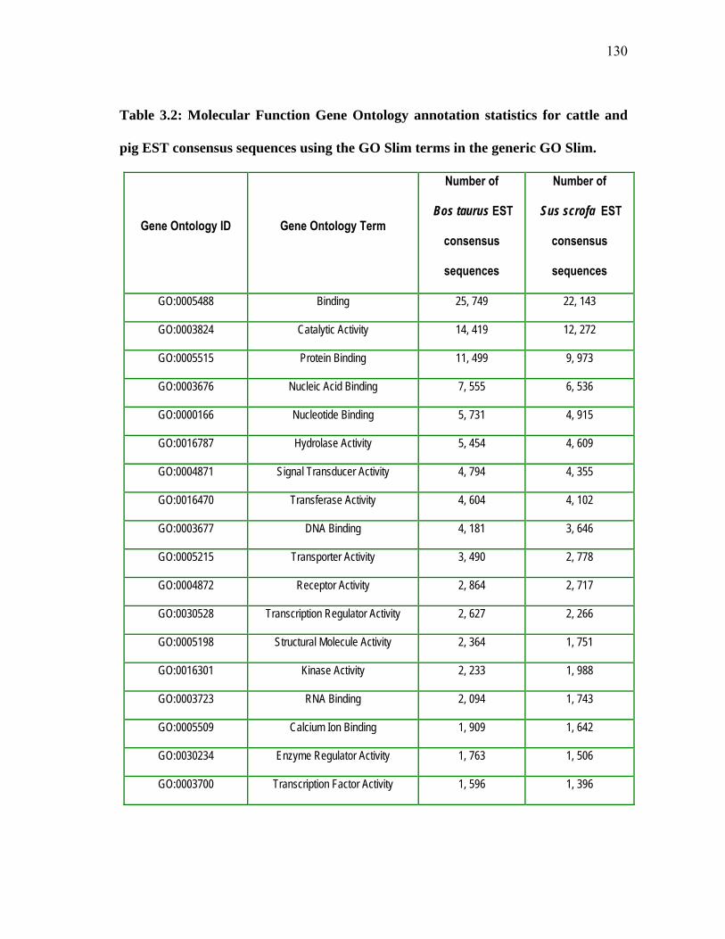
130
Table 3.2: Molecular Function Gene Ontology annotation statistics for cattle and
pig EST consensus sequences using the GO Slim terms in the generic GO Slim.
Gene Ontology ID Gene Ontology Term
Number of
Bos taurus EST
consensus
sequences
Number of
Sus scrofa EST
consensus
sequences
GO:0005488 Binding 25, 749 22, 143
GO:0003824 Catalytic Activity 14, 419 12, 272
GO:0005515 Protein Binding 11, 499 9, 973
GO:0003676 Nucleic Acid Binding 7, 555 6, 536
GO:0000166 Nucleotide Binding 5, 731 4, 915
GO:0016787 Hydrolase Activity 5, 454 4, 609
GO:0004871 Signal Transducer Activity 4, 794 4, 355
GO:0016470 Transferase Activity 4, 604 4, 102
GO:0003677 DNA Binding 4, 181 3, 646
GO:0005215 Transporter Activity 3, 490 2, 778
GO:0004872 Receptor Activity 2, 864 2, 717
GO:0030528 Transcription Regulator Activity 2, 627 2, 266
GO:0005198 Structural Molecule Activity 2, 364 1, 751
GO:0016301 Kinase Activity 2, 233 1, 988
GO:0003723 RNA Binding 2, 094 1, 743
GO:0005509 Calcium Ion Binding 1, 909 1, 642
GO:0030234 Enzyme Regulator Activity 1, 763 1, 506
GO:0003700 Transcription Factor Activity 1, 596 1, 396

131
Table 3.3: Cellular Component Gene Ontology annotation statistics for cattle and
pig EST consensus sequences using the GO Slim terms in the generic GO Slim.
Gene Ontology ID Gene Ontology Term
Number of
Bos taurus EST
consensus
sequences
Number of
Sus scrofa EST
consensus
sequences
GO:0005623 Cell 26, 772 22, 754
GO:0005622 Intracellular 19, 802 16, 700
GO:0043226 Organelle 16, 271 13, 788
GO:0005737 Cytoplasm 10, 015 8, 239
GO:0005634 Nucleus 8, 787 7, 581
GO:0043234 Protein Complex 5, 389 4, 252
GO:0005886 Plasma Membrane 3, 175 2, 668
GO:0005576 Extracellular Region 2, 950 2, 461
GO:0005856 Cytoskeleton 2, 192 1, 843
GO:0005739 Mitochondrion 2, 058 1, 741
GO:0005615 Extracellular Space 1, 583 1, 270
GO:0005783 Endoplasmic Reticulum 1, 459 1, 217
GO:0005829 Cytosol 1, 148 823
GO:0005794 Golgi Apparatus 1, 090 1, 036
GO:0005840 Ribosome 1, 038 720
GO:0005654 Nucleoplasm 727 628
GO:0005694 Chromosome 705 667
GO:0005578 Extracellular Matrix 682 601

132
The findings from Tables 3.1, 3.2 and 3.3 after profiling the cattle and pig
transcriptomes in the “Biological Process”, “Molecular Function” and “Cellular
Component” namespaces of Gene Ontology are illustrated in Figures 3.12, 3.13 and
3.14. Given below is a summary of the findings from Tables 3.1, 3.2 and 3.3.
Biological Process profile
Figure 3.12 depicts the Biological Process Gene Ontology profile for the cattle
and the pig transcriptomes. The largest Biological Process GO category in both the
transcriptomes was the ‘physiological process’ category with approximately 67% of both
the cattle and pig EST gene products coming under it (27, 477 Cattle EST Consensus
sequences and 23, 315 Pig EST Consensus sequences). The next largest categories in the
Biological Process GO were the EST gene products pertaining to the ‘metabolism’
category with ~47% of cattle and pig EST gene products in it (19,374 Cattle EST
Consensus sequences and 16,435 Pig EST Consensus sequences). The ‘metabolism’
category encompasses ‘primary metabolism’ (~42% of cattle and pig EST gene
products), ‘protein metabolism’ (~20% of cattle and pig EST gene products), and
‘nucleic acid metabolism’ (~20% of cattle and pig EST gene products). Among the other
GO terms in the Biological Process namespace, the ‘transport’ category has
approximately 17% of cattle and pig EST gene products, and the ‘stress response’ as
well as the ‘biotic stimulus response’ categories having approximately 6% of cattle and
pig EST gene products.

133
Figure 3.12: Biological Process Gene Ontology (GO) profiles for cattle and pig EST consensus sequences. Assignment to the different GO Slim terms for cattle (top panel) and pig (bottom panel) EST consensus sequences normalized on number of sequences having GO annotations.

134
Molecular Function profile
Figure 3.13 depicts the Molecular Function Gene Ontology profile for the cattle
and the pig transcriptomes. The largest Molecular Function GO category in both the
transcriptomes was the ‘binding’ category with approximately 63% of both the cattle and
pig EST gene products coming under it (25,749 Cattle EST Consensus sequences and
22,143 Pig EST Consensus sequences). The ‘binding’ category encompasses the
following categories: ‘protein binding’ (~28% of cattle and pig EST gene products),
‘nucleic acid binding’ (~19% of cattle and pig EST gene products), ‘nucleotide binding’
(~14% of cattle and pig EST gene products), ‘DNA binding’ (~10% of cattle and pig
EST gene products) and ‘RNA binding’ (~5% of cattle and pig EST gene products). The
next largest category in the Molecular Function GO was the ‘catalytic activity’ category
with ~35% of cattle and pig EST gene products in it (14,419 Cattle EST Consensus
sequences and 12,272 Pig EST Consensus sequences). The ‘catalytic activity’ GO
encompasses the ‘hydrolase activity’ (~13% of cattle and pig EST gene products)
category and the ‘transferase activity’ (~11% of cattle and pig EST gene products)
category. Among the other GO terms in the Molecular Function namespace, the ‘signal
transducer activity’ category has ~12% of cattle and pig EST gene products, the
‘transporter activity’ category has ~9% of cattle and pig EST gene products, and the
‘receptor activity’ as well as the ‘transcription regulator activity’ categories mapping to
approximately 6-8% of the cattle and pig EST gene products.

135
Figure 3.13: Molecular Function Gene Ontology (GO) profiles for cattle and pig EST consensus sequences. Assignment to the different GO Slim terms for cattle (top panel) and pig (bottom panel) EST consensus sequences normalized on number of sequences having GO annotations.
136
Cellular Component profile
Figure 3.14 depicts the Cellular Component Gene Ontology profile for the cattle
and the pig transcriptomes. The ‘cell’ category was the largest Cellular Component GO
category in both the transcriptomes with approximately 65% of both the cattle and pig
EST gene products coming under it (26,772 Cattle EST Consensus sequences and
22,754 Pig EST Consensus sequences). The ‘cell’ category encompasses the following
categories: ‘intracellular’ (~48% of cattle and pig EST gene products), ‘cytoplasm’
(~24% of cattle and pig EST gene products), ‘nucleus’ (~21% to ~22% of cattle and pig
EST gene products), ‘plasma membrane’ (~8% of cattle and pig EST gene products) and
‘cytoskeleton’ (~5% of cattle and pig EST gene products). The next largest categories in
the Cellular Component GO was the ‘organelle’ category with ~39% to ~40% of cattle
and pig EST gene products in it (16,271 Cattle EST Consensus sequences and 13,788
Pig EST Consensus sequences) and the ‘protein complex’ category with ~12% to ~13%
of cattle and pig EST gene products in it (5,389 Cattle EST Consensus sequences and
4,252 Pig EST Consensus sequences).

137
Figure 3.14: Cellular Component Gene Ontology (GO) profiles for cattle and pig EST consensus sequences. Assignment to the different GO Slim terms for cattle (top panel) and pig (bottom panel) EST consensus sequences normalized on number of sequences having GO annotations.
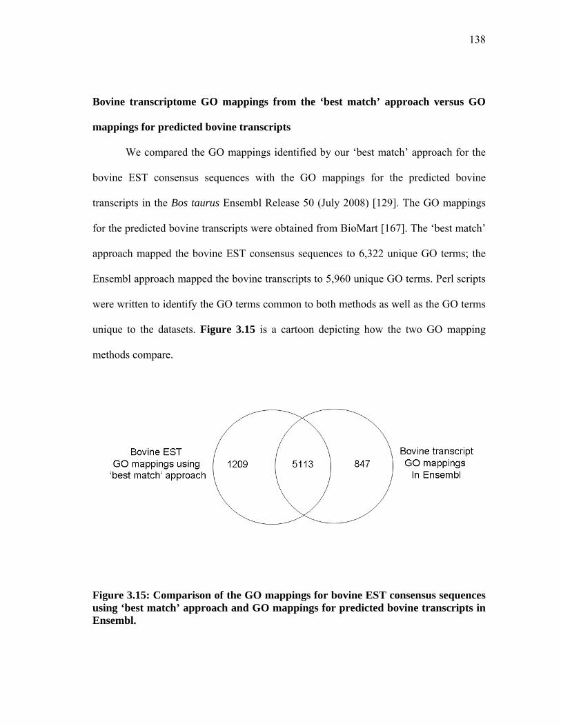
138
Bovine transcriptome GO mappings from the ‘best match’ approach versus GO
mappings for predicted bovine transcripts
We compared the GO mappings identified by our ‘best match’ approach for the
bovine EST consensus sequences with the GO mappings for the predicted bovine
transcripts in the Bos taurus Ensembl Release 50 (July 2008) [129]. The GO mappings
for the predicted bovine transcripts were obtained from BioMart [167]. The ‘best match’
approach mapped the bovine EST consensus sequences to 6,322 unique GO terms; the
Ensembl approach mapped the bovine transcripts to 5,960 unique GO terms. Perl scripts
were written to identify the GO terms common to both methods as well as the GO terms
unique to the datasets. Figure 3.15 is a cartoon depicting how the two GO mapping
methods compare.
Figure 3.15: Comparison of the GO mappings for bovine EST consensus sequences using ‘best match’ approach and GO mappings for predicted bovine transcripts in Ensembl.

139
Figure 3.15 reveals that the two methods have 5113 GO terms in common and
~1000 GO terms unique to either set. We believe that the ~1000 or so GO terms unique
to either set could be due to the fact that the GO annotations for the Bovine Genome
project are ongoing and not yet complete. The ‘best match’ approach of GO annotations
for the bovine EST consensus sequences does not rely on GO mappings from the bovine
genome; instead, GO annotations are transferred to the bovine EST consensus sequence
based on the vertebrate protein match found using FASTX and using the species
precedence order described earlier. In spite of the differences in the approach taken by
the two methods for the GO mappings, the fact that there are 5113 GO terms are in
common between the two methods signifies that the procedure of transferring GO
annotations using the ‘best match’ approach can be relied upon for species that do not
have complete genome sequences and/or do not have GO mappings derived from a
complete genome sequence being available.
CONCLUSIONS
Bos taurus (cattle) and Sus scrofa (pig) are important livestock species that serve
as candidate animal models for biomedical research. In the absence of availability of
completed genomes for the Bos taurus and Sus scrofa species, very less information
exists about the genes and the gene products. In this scenario, EST datasets were utilized
to obtain insights of the functions encoded in the cattle and the pig transcriptomes using
computational predictions.
140
Anonymous ESTs are of limited value unless connected to function, thereby
necessitating the need for annotated datasets. The Livestock EST Gene Family Database
consists of cattle and pig ESTs clustered into gene families using the vertebrate
proteomes in the Ensembl database as a framework for assembly and translation. Cattle
and Pig ESTs were electronically annotated making use of the rich annotations of the
vertebrate proteomes; these annotated datasets would help researchers to deal with the
volume of information, and to utilize the information embedded in the gene expression
data gathered from assembling the EST datasets. These annotations would immensely
aid the livestock community in narrowing down the gamut of direct experiments needed
to verify function. The database has a user-friendly web interface and can be searched in
a number of ways: Cattle/Pig EST GenBank identifiers (GI or Accession), Gene
Ontology Accession to obtain information about the vertebrate protein family, related
EST members and other annotations.
The Livestock EST Gene Family Database is the first of its kind where ESTs
with similar functions in more than one species are grouped together in the same gene
family. This information comes in handy when one wants to get a listing of ESTs from
different species performing the same function. To do so, one could search the database
using an EST from species 1; obtain the Protein Family Id for that EST. Upon searching
the database using the Protein Family Id as the query, one can get a listing of all the
ESTs from different species belonging to that Protein Family Id.
The Livestock EST Gene Family Database is also the first of its kind that
incorporates an AmiGO [170] like search strategy to transitively annotate EST gene

141
products with a GO accession and all its descendants. The AmiGO database houses gene
product annotations from model organisms whose complete genome sequences are
known and AmiGO does not house GO annotations for EST gene products. Searching by
GO accession on the Livestock EST Gene Family Database will retrieve the complete
descendant information for the GO accession and give a mapping of the different
livestock EST contigs/singletons associated with the complete GO descendant tree
starting from that GO Accession. This search feature will come in handy for users who
want to get a complete profile of the cattle and pig EST gene products associated with a
particular GO Accession.
The GO terms mapped to the bovine EST consensus sequences identified by the
‘best match’ approach were compared to the GO terms mapped to the bovine transcripts
by Ensembl. Despite the different strategies used by the two methods, the findings reveal
that the ‘best match’ approach compares well with the Ensembl approach and can be
used reliably for species that do not have complete genome sequences and/or do not
have GO mappings derived from a complete genome sequence being available.
A GO Slim analysis was performed to functionally categorize the cattle and pig
transcriptomes within arbitrary coarser (parent) levels of the three independent
ontologies - biological process, molecular function and cellular component - and helped
in the identification of the roles of the different EST gene products. The GO Slim
analysis helped profile the cattle and pig transcriptomes by conveying biological
meaning at a coarser level, thereby making up for inconsistencies like categorization
errors and/or incomplete coverage of certain categories.
142
The work described in this chapter provides an invaluable resource to explore the
orthologous relationships and evolutionary analysis of the genes and gene families in
cattle and pig, and for functional genomics. The computational function predictions of
the cattle and the pig transcriptomes would help in obtaining a first-order approximation
of the molecular function of the proteins encoded and come in handy while prioritizing
experimental investigations.
143
CHAPTER IV
DESCRIPTION OF A PHYLOGENOMIC ANNOTATION PIPELINE FOR
COMPUTATIONAL FUNCTION PREDICTIONS OF THE Bos taurus AND
Sus scrofa TRANSCRIPTOMES
SYNOPSIS
In this chapter, EST consensus sequences, which had been generated from cattle
and pig ESTs after grouping ESTs into gene families, were combined with proteins in
their respective protein family, and subject to multiple sequence alignment and
phylogenetic analysis. The phylogenetic trees obtained were then analyzed using a
subtree neighbors approach to predict function of the cattle ad pig ESTs consensus
sequences. This analysis was able to identify function for ~23% of the Livestock EST
gene products. The remaining ~77% of the sequences were excluded due to various
reasons that include, but are not restricted to: a) belonging to families with 50 or more
members, b) ambiguous regions in the multiple sequence alignment, c) failure to match
tree resolving criteria in the consensus phylogenetic tree reconstruction after
bootstrapping, d) tree ambiguity problems. This work thus outlines the processes
required for phylogenomic annotation and identifies the technical/biological pitfalls of
the same. This work, to our knowledge, is the first of its kind where phylogenomic
inference has been used in predicting functions for EST gene products, and the function
predictions of the uncharacterized cattle/pig EST gene products using this approach
would help reduce the number of direct experiments required to verify function.

144
BACKGROUND
Orthologs are evolutionary counterparts derived from a single ancestral gene in
the last common ancestor of species being compared [70-72] . Orthologs are likely to
have equivalent or similar functions because of their phylogenetically close
relationships; however, function is not part of the definition. The high level of function
conservation between orthologs makes orthology relevant for protein function
prediction.
Phylogenetic analysis helps improve function predictions by incorporating an
evolutionary perspective. Phylogenomics combines evolutionary and comparative
genomic analysis into a single composite approach [1], and involves inferring function
of a unknown sequence (protein) in the larger context of a protein family based on
evolutionary relationships [32, 39, 53, 77]. In this approach, a phylogenetic tree is
constructed following multiple sequence alignment of the different members of a protein
family. As a result, the various members of the family are segregated into subfamilies;
each subfamily representing a functionally and evolutionarily distinct group of
homologous proteins with similar functions and activities. The tree topology is then
analyzed and the phylogenetic information encoded in the subfamily (or subtree)
structure is used to infer likely functions for the uncharacterized members of the protein
family. Since function is conserved within orthologous subfamilies [82], uncharacterized
genes can be assigned predicted function based on the subfamily in which they are
placed.

145
Making accurate function predictions is a key step and these predictions have
become increasingly important as numerous sequences are being generated with little or
no accompanying experimentally determined information regarding the function they
encode. Bos taurus (cattle) and Sus scrofa (pig) represent evolutionary clades distinct
from the primates and rodents, and therefore are good candidate animal models for
biomedical research due to parallels with humans. The genome sequences for these
species are in different stages of completion [10, 12], and in this scenario Expressed
Sequence Tags represent a good alternative to indentify the genes and the functions
encoded in the genome.
Overview of the work in this chapter
In this chapter, we use a phylogenomic approach to predict the functions encoded
in the Bos taurus (cattle) and Sus scrofa (pig) transcriptomes. Cattle and pig ESTs were
first grouped into gene families using the vertebrate protein family clusters obtained
from an in-house clustering algorithm developed in our lab. Phylogenetic analysis of the
protein family clusters results in subdivisions of groups containing orthologs and
paralogs, each group representing distinct subfamilies.
As part of the TAMUClust EST clustering pipeline, cattle and pig ESTs were
grouped into gene/protein families using the Ensembl protein families as the framework.
The different proteins and the EST gene products in each protein family are passed
through a multiple sequence alignment and phylogenetic analysis pipeline. The resulting
phylogenetic trees were analyzed for their tree topology and the functions of the

146
uncharacterized EST gene family members were predicted by their positions on the
phylogenetic tree involving other member(s) of the subgroup/subfamily.
To our knowledge, this is the first time that phylogenomic analysis, and that too
on a large scale, has been used in predicting functions for EST gene products. This
analysis helps obtain improved function predictions of the uncharacterized EST gene
family members in cattle and pig, and would thereby provide the livestock community
with an invaluable resource to verify function of the EST gene products by designing
experiments based on these predictions.
MATERIALS AND METHODS
Assembling a dataset
One of the preliminary requirements for constructing a phylogenetic tree is
building the dataset. Given below are the steps used in assembling a protein family
dataset comprising of Ensembl vertebrate proteomes and bovine/porcine translated EST
Contig/Singleton sequences:
1) Bos taurus and Sus scrofa ESTs were clustered into gene families using Dr. Elsik’s
clustering algorithm as described in Chapter II. This clustering algorithm is a two
step process and uses the vertebrate proteomes in the Ensembl database as a
framework to assemble and translate the ESTs. A total of 219,433 Ensembl
vertebrate proteins from Homo sapiens, Mus musculus, Rattus norvegicus, Gallus
gallus, Danio rerio, Takifugu rubripes and Tetraodon nigroviridis were clustered
into 10,092 protein families. The vertebrate protein families served as a framework
147
to group the Bos taurus and Sus scrofa ESTs into gene families using Dr. Elsik’s
algorithm as described in Chapter II. 308,132 bovine ESTs were grouped into
46,731 EST Clusters (24,665 contigs and 22,066 singletons); 238,691 porcine ESTs
were grouped into 39,641 EST Clusters (20,951 contigs and 18,690 singletons).
2) The “best match” Ensembl vertebrate protein for every EST Contig/Singleton was
determined using the pipeline mentioned in Chapter III. The ‘protein2dna’ model of
the Exonerate [171, 172] program in conjunction with the “ryo” (roll your own)
output option was used to translate the EST Contig/Singleton using the “best match”
Ensembl vertebrate protein as the framework. The ‘protein2dna’ model compares a
protein sequence to a DNA sequence while incorporating all the appropriate gaps
and frameshifts. Perl scripts were written to automate the procedure and to parse the
Exonerate outputs to generate a fasta file of the translated EST Contig/Singleton.
3) Perl scripts were written to make directories of protein families generated by Dr.
Elsik’s single-linkage and average-linkage clustering results of the Ensembl
vertebrate proteins. Each directory (protein family) contains fasta files of the
different Ensembl vertebrate proteins assigned to that protein family by Dr. Elsik’s
clustering algorithm.
4) Perl scripts were written to first identify the protein family to which a translated EST
Contig/Singleton (from Step 2 above) belongs and then to assign it to its respective
protein family directory (from Step 3 above).
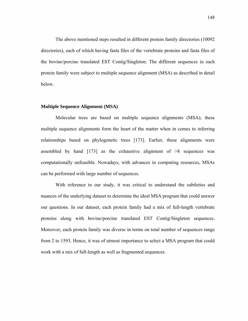
148
The above mentioned steps resulted in different protein family directories (10092
directories), each of which having fasta files of the vertebrate proteins and fasta files of
the bovine/porcine translated EST Contig/Singleton. The different sequences in each
protein family were subject to multiple sequence alignment (MSA) as described in detail
below.
Multiple Sequence Alignment (MSA)
Molecular trees are based on multiple sequence alignments (MSA); these
multiple sequence alignments form the heart of the matter when in comes to inferring
relationships based on phylogenetic trees [173]. Earlier, these alignments were
assembled by hand [173] as the exhaustive alignment of >8 sequences was
computationally unfeasible. Nowadays, with advances in computing resources, MSAs
can be performed with large number of sequences.
With reference to our study, it was critical to understand the subtleties and
nuances of the underlying dataset to determine the ideal MSA program that could answer
our questions. In our dataset, each protein family had a mix of full-length vertebrate
proteins along with bovine/porcine translated EST Contig/Singleton sequences.
Moreover, each protein family was diverse in terms on total number of sequences range
from 2 to 1593. Hence, it was of utmost importance to select a MSA program that could
work with a mix of full-length as well as fragmented sequences.
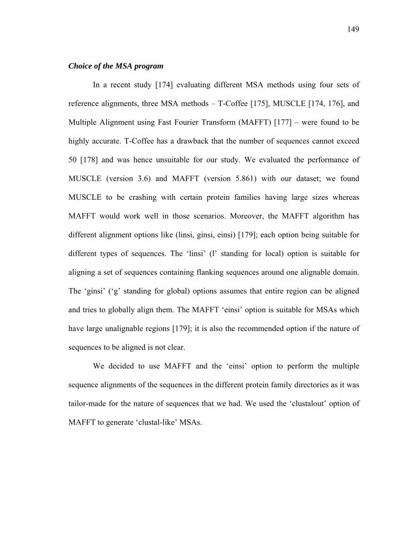
149
Choice of the MSA program
In a recent study [174] evaluating different MSA methods using four sets of
reference alignments, three MSA methods – T-Coffee [175], MUSCLE [174, 176], and
Multiple Alignment using Fast Fourier Transform (MAFFT) [177] – were found to be
highly accurate. T-Coffee has a drawback that the number of sequences cannot exceed
50 [178] and was hence unsuitable for our study. We evaluated the performance of
MUSCLE (version 3.6) and MAFFT (version 5.861) with our dataset; we found
MUSCLE to be crashing with certain protein families having large sizes whereas
MAFFT would work well in those scenarios. Moreover, the MAFFT algorithm has
different alignment options like (linsi, ginsi, einsi) [179]; each option being suitable for
different types of sequences. The ‘linsi’ (l’ standing for local) option is suitable for
aligning a set of sequences containing flanking sequences around one alignable domain.
The ‘ginsi’ (‘g’ standing for global) options assumes that entire region can be aligned
and tries to globally align them. The MAFFT ‘einsi’ option is suitable for MSAs which
have large unalignable regions [179]; it is also the recommended option if the nature of
sequences to be aligned is not clear.
We decided to use MAFFT and the ‘einsi’ option to perform the multiple
sequence alignments of the sequences in the different protein family directories as it was
tailor-made for the nature of sequences that we had. We used the ‘clustalout’ option of
MAFFT to generate ‘clustal-like’ MSAs.

150
Phylogenetic analysis
There are three methods – maximum parsimony, maximum likelihood, and
distance – to determine the evolutionary tree or trees that best account for the observed
variation in a group of sequences.
1) Maximum parsimony (MP) predicts the evolutionary tree that minimizes the number
of steps required to generate the observed variation in the sequences from common
ancestral sequences. Analysis is performed on every single column of the MSA and
for each aligned position, phylogenetic trees that require smallest number of
evolutionary changes are found. This is repeated for every position in the sequence
alignment. Finally, only those trees that produce smallest amount of changes overall
for all sequence positions are determined. Because the maximum parsimony method
tries to fit all possible trees to the data, this method is best suited [97] for analysis
involving sequences that are quite similar and is limited to small number (<12) of
sequences in a MSA. The MP method is also not suitable for sequences from large
evolutionary distances as it does not take into account a model of evolution.
2) Maximum likelihood (ML) methods start with a simple model of rates of
evolutionary changes in sequences and tree models that represent a pattern of
evolutionary change, and then adjust the model until a best fit for the observed data
is found. Similar to the MP method, ML methods also perform analysis on each
column of the alignment. The ML method resembles the MP method in that trees
with the least number of changes will be the most likely. However, the ML method
allows one to evaluate tress with variations in mutation rates in different lineages, or
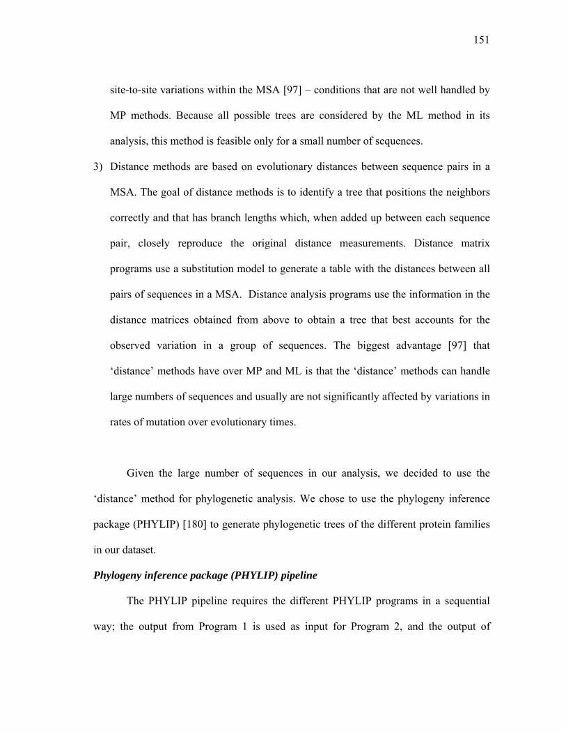
151
site-to-site variations within the MSA [97] – conditions that are not well handled by
MP methods. Because all possible trees are considered by the ML method in its
analysis, this method is feasible only for a small number of sequences.
3) Distance methods are based on evolutionary distances between sequence pairs in a
MSA. The goal of distance methods is to identify a tree that positions the neighbors
correctly and that has branch lengths which, when added up between each sequence
pair, closely reproduce the original distance measurements. Distance matrix
programs use a substitution model to generate a table with the distances between all
pairs of sequences in a MSA. Distance analysis programs use the information in the
distance matrices obtained from above to obtain a tree that best accounts for the
observed variation in a group of sequences. The biggest advantage [97] that
‘distance’ methods have over MP and ML is that the ‘distance’ methods can handle
large numbers of sequences and usually are not significantly affected by variations in
rates of mutation over evolutionary times.
Given the large number of sequences in our analysis, we decided to use the
‘distance’ method for phylogenetic analysis. We chose to use the phylogeny inference
package (PHYLIP) [180] to generate phylogenetic trees of the different protein families
in our dataset.
Phylogeny inference package (PHYLIP) pipeline
The PHYLIP pipeline requires the different PHYLIP programs in a sequential
way; the output from Program 1 is used as input for Program 2, and the output of

152
Program 2 is used as input for Program 3, and so on. The perl modules Bio::AlignIO and
Bio::SimpleAlign from the BioPerl toolkit [181] were used in perl scripts to convert the
MSAs from a ‘clustal-like’ format to a ‘phylip infile’ format required by PHYLIP. This
‘phylip infile’ was passed though a PHYLIP pipeline as detailed below:
1. Seqboot: Seqboot is a general bootstrapping and data set translation tool which
generates multiple data sets that are resampled versions of the input data set. The
input dataset can be resampled in many ways: bootstrapped, jackknifed, or
permuted. We used Seqboot with the default settings to generate 100 bootstrapped
datasets. Bootstrapping tests whether the entire dataset is supporting the tree or if
the tree is a marginal winner among many equally possible alternatives.
Bootstrapping is done by taking random subsamples of the dataset. Building trees
from these and calculating the frequency with which various parts of the tree are
reproduced in each of the random subsamples. Seqboot requires the input file to be
called ‘infile’ and produces an output file called ‘outfile’. The file called ‘outfile’
has to be renamed to ‘infile’ before it can be used as an input for ProtDist.
2. ProtDist: ProtDist is a ‘distance matrix’ program which uses amino acid
replacement models on protein sequences to compute a distance matrix. The
distance for each pair of species is the estimated total branch length between the
two species, and this distance can be used by ‘distance analysis’ programs like
Fitch to generate trees. We used the Jones-Taylor-Thornton (JTT) model [182] –
the default model in this program. We changed the default settings on ProtDist
using the ‘M’ option to analyze 100 datasets to account for the fact that we had
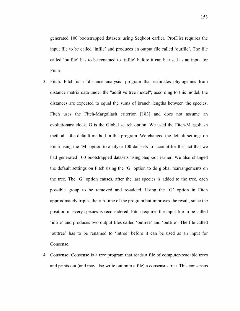
153
generated 100 bootstrapped datasets using Seqboot earlier. ProtDist requires the
input file to be called ‘infile’ and produces an output file called ‘outfile’. The file
called ‘outfile’ has to be renamed to ‘infile’ before it can be used as an input for
Fitch.
3. Fitch: Fitch is a ‘distance analysis’ program that estimates phylogenies from
distance matrix data under the "additive tree model"; according to this model, the
distances are expected to equal the sums of branch lengths between the species.
Fitch uses the Fitch-Margoliash criterion [183] and does not assume an
evolutionary clock. G is the Global search option. We used the Fitch-Margoliash
method – the default method in this program. We changed the default settings on
Fitch using the ‘M’ option to analyze 100 datasets to account for the fact that we
had generated 100 bootstrapped datasets using Seqboot earlier. We also changed
the default settings on Fitch using the ‘G’ option to do global rearrangements on
the tree. The ‘G’ option causes, after the last species is added to the tree, each
possible group to be removed and re-added. Using the ‘G’ option in Fitch
approximately triples the run-time of the program but improves the result, since the
position of every species is reconsidered. Fitch requires the input file to be called
‘infile’ and produces two output files called ‘outtree’ and ‘outfile’. The file called
‘outtree’ has to be renamed to ‘intree’ before it can be used as an input for
Consense.
4. Consense: Consense is a tree program that reads a file of computer-readable trees
and prints out (and may also write out onto a file) a consensus tree. This consensus
154
tree serves as the consensus from amongst the different phylogenetic trees
generated from the bootstrapped datasets (100 datasets in our case). Out of the four
consensus methods used by this program, we chose to use the ‘majority rule
extended’ (MRe) method – the default method in this program. The MRe method
first includes all sequences that appear in more than 50% of the trees. The program
then considers the other sets of sequences in order of the frequency with which
they have appeared, adding to the consensus tree any which are compatible with it
until the tree is fully resolved. Consense requires the input file to be called ‘intree’
and produces two output files called ‘outtree’ and ‘outfile’. The ‘outtree’ is a tree
file where the trees are represented in a linear form by a series of nested
parentheses, enclosing names and separated by commas. This type of
representation is called the ‘Newick’ format [184] and the originator of this format
was the English mathematician Arthur Cayley; the pattern of the parentheses in the
‘Newick’ format indicates the tree topology.
Making images of phylogenetic trees
The perl module Bio::Tree::Draw::Cladogram from the BioPerl toolkit [181] was
used in perl scripts to parse the phylogenetic tree files and obtain a cladogram of the tree
in postscript format. A cladogram is a tree that depicts the tree topology by means of
ancestor-descendant relationships. The postscript cladogram files were converted to pdf
using the unix utility ‘ps2pdf’.
155
RESULTS AND DISCUSSION
Multiple Sequence Alignment (MSA) editing
Most multiple sequence alignments are constructed by the ‘progressive sequence
alignment’ method [185]; this method begins with the construction of a crude ‘guide
tree’ which involves pairwise comparison of all sequences to determine the order in
which sequences are progressively added to build the alignment. With this ‘guide tree’,
the MSA program starts with the most similar sequences, builds an alignment and
progressively adds more dissimilar sequences. Each alignment position is assumed to
include residues that share common ancestry among species; hence it is important to edit
the MSA to remove regions of ambiguous alignment from the MSAs before
phylogenetic analysis.
We edited the MSAs to exclude any ambiguous regions and include only the
densest portions over a given window length, which is the larger of these two indices:
(i) length of 100
(ii) 90% of the length of the longest sequence in the MSA
We then trim the alignment to include this window alone; in this process, the
sequences which do not satisfy the above mentioned criteria are excluded from the
phylogenetic analysis. The statistics pertaining to number of vertebrate proteins,
bovine/porcine contigs/singletons that passed our MSA editing criteria are detailed in
Table 4.1.

156
Entire dataset or large enough dataset
Large datasets often bring up an interesting dilemma; whether to include all the
data or to include data that is large and representative enough to answer the biological
question being asked within a reasonable timeframe. In this tradeoff, we decided on the
latter and we chose to run the PHYLIP pipeline only on those families which have ≤50
sequences in the edited MSA. The entire process (MSA, PHYLIP pipeline on protein
families having ≤50 sequences) took ~4-5 months with the different jobs running in
parallel on a computer cluster having 12 worker nodes.
Table 4.1: Comparative statistics of the number of sequences present in the original
and final multiple sequence alignment.
Present in
original MSA
Not Included in
final (edited) MSA
Included in final
(edited) MSA
Vertebrate proteins 133,874 11,543 122,331
Translated bovine contigs 24, 665 8,778 15,887
Translated bovine singletons 22, 006 10,636 11,370
Translated porcine contigs 20, 951 7,211 13,740
Translated porcine singletons 18,690 9,568 9,122
Total number of sequences 220,186 47,736 172,450

157
Phylogenetic tree analysis
Phylogenetic analysis is a powerful tool for interpreting molecular data.
Prediction of trees produced by ‘distance’ methods can be improved by rerooting the
trees using an ‘outgroup’ sequence. The ‘outgroup’ sequence is one that is more
distantly related to the other sequences than they are to each other; the ‘outgroup’ acts as
an external reference and aids in correctly arranging the other sequences.
Choosing an outgroup
In our analysis, each protein family can have sequences from a maximum of nine
species (translated EST Contig/Singleton sequences from cattle and pig, in addition to
the protein sequences from the seven vertebrate species). The number of species in each
tree would vary depending on the species represented in each protein family. In this
scenario, each tree had to be first analyzed to determine the ‘outgroup’ and then rerooted
using the ‘outgroup’. Keeping in mind that our analysis focused on determining
annotations using a phylogenomic pipeline for ‘cattle’ and ‘pig’ EST gene products, the
‘outgroup’ was determined from amongst the various proteomes using this order of
precedence: Takifugu rubripes, Tetraodon nigroviridis, Danio rerio, Gallus gallus,
Rattus norvegicus, Mus musculus and Homo sapiens. For example, if a phylogenetic
tree has sequences from Takifugu rubripes, then Takifugu rubripes was used as the
‘outgroup’. If the tree does not have Takifugu rubripes sequences, the next species using
the order of precedence mentioned above was used as the ‘outgroup’.
Perl scripts incorporating the perl module Bio::TreeIO from the BioPerl toolkit
[181] were written to navigate the tree and to determine the ‘outgroup’ using the strategy

158
mentioned above. Outgroups were determined for every phylogenetic tree; in other
words, outgroups were determined for every protein family that got included in the
phylogeny analysis. With this knowledge of the ‘outgroup’, all the phylogenetic trees
were rerooted, subject to a ‘subtree neighbors’ approach to determine orthologs and
subsequent function annotation of the bovine/porcine EST gene products.
Livestock EST gene products function classification using subfamily annotation
Subtree neighbors approach for assigning predicted function
In the subtree neighbors approach, multiple seqeunce alignment (MSA) of
proteins in a protein family is performed in the lead up to phylogenetic tree construction.
Following this, the tree topology is analyzed and sequences without known function can
be assigned a predicted function on the basis of other sequences in the subtree containing
the sequence with unknown function.
We adopt this ‘subtree neighbors’ approach to identify the most recent diverging
sequence from a different species with reference to the sequence (bovine/porcine) whose
function we are predicting. In other words, by using the subtree neighbors approach, we
are finding the best ortholog from amongst many possible orthologs. Using this
approach, we end up identifying orthologs for a particular bovine/porcine EST gene
product based on the subfamily the EST gene product gets grouped with in the
phylogenetic tree. The EST gene product is then assigned predicted function from
amongst one of the ortholog(s). Here is the pseudocode used in this study to determine
the ortholog(s) for a bovine/porcine EST gene product:
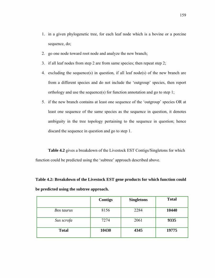
159
1. in a given phylogenetic tree, for each leaf node which is a bovine or a porcine
sequence, do;
2. go one node toward root node and analyze the new branch;
3. if all leaf nodes from step 2 are from same species; then repeat step 2;
4. excluding the sequence(s) in question, if all leaf node(s) of the new branch are
from a different species and do not include the ‘outgroup’ species, then report
orthology and use the sequence(s) for function annotation and go to step 1;
5. if the new branch contains at least one sequence of the ‘outgroup’ species OR at
least one sequence of the same species as the sequence in question, it denotes
ambiguity in the tree topology pertaining to the sequence in question; hence
discard the sequence in question and go to step 1.
Table 4.2 gives a breakdown of the Livestock EST Contigs/Singletons for which
function could be predicted using the ‘subtree’ approach described above.
Table 4.2: Breakdown of the Livestock EST gene products for which function could
be predicted using the subtree approach.
Contigs Singletons Total
Bos taurus 8156 2284 10440
Sus scrofa 7274 2061 9335
Total 10430 4345 19775

160
Given that orthologs are sequences derived from a single ancestral gene in the
last common ancestor of the species being compared, there is no requirement for
orthology to be a one-to-one relationship. In case of one or more duplication events
happening after speciation, it can result in one-to-one, one-to-many, many-to-one and
many-to-many orthologous relationships.
Usage notes for the phrase ‘one-to-many orthologous relationship’ in this work
In the ensuing discussions in this chapter, we would like to mention that the
phrase ‘one-to-many orthologous relationship’ is not used in the evolutionary sense;
instead, it is used in an algorithmic sense with reference to the subtree neighbors
method. From an evolutionary standpoint, the ‘one-to-many orthologous relationship’
would reflect a scenario where gene duplication in a family (say with members A, B, C)
occurs after a speciation event in one lineage or in both lineages independently (lineage-
specific expansion); in these situations, the functional correspondence between the two
orthologous families is less straightforward than it is between one-to-one orthologs [24].
Instead, one can only state the members (say A1, B1, C1) of a family in lineage 1 are co-
orthologous to the members (say A2, B2, C2) of the same family in lineage 2.
From the subtree neighbors algorithmic standpoint, ‘one-to-many orthologous
relationships’ encompass these three scenarios:
1. the bovine/porcine EST gene product is orthologous to multiple splice isoforms
produced by the same gene in a species as well as duplicated gene products in a
species resulting from lineage specific expansions;

161
2. the bovine/porcine EST gene product is part of multiple one-to-one orthologous
relationships with proteins in more than one species; and
3. combination of the above-mentioned scenarios ‘1’ and ‘2’.
The ‘subtree’ approach mentioned above was used to determine the best ortholog
for the bovine/porcine EST gene product from amongst a set of orthologs. In cases
where a one-to-one orthology relationship could not be detected because of one or more
duplication events happening after speciation, we term the orthologous relationships as
‘one-to-many’ from the algorithmic standpoint as specified above. We do not attempt to
distinguish between these three scenarios: multiple splice isoforms produced by the same
gene in a species, duplicated gene products in a species as a result of lineage specific
expansions and multiple one-to-one orthologous relationship with proteins in more than
one species. The most recent diverging sequence(s) from a different species with
reference to the bovine/porcine EST gene product identified by the ‘subtree’ method was
used for assigning predicted function and for annotation transfer. Using this approach,
we were able to predict function for 19775 Livestock EST gene products and this
resulted in a mix of gene products which were part of one-to-one orthologous
relationships as well as one-to-many orthologous relationships from the ‘subtree
neighbors’ algorithmic standpoint.
From amongst the 19775 Livestock EST gene products for which function could
be predicted using the above approach, 13895 of them had a one-to-one orthologous
relationship. Figure 4.1 depicts the statistics pertaining to the different one-to-many

162
orthologous relationships found for the remaining 5880 Livestock EST gene products for
which putative orthologs could be identified.
Figure 4.1: One-to-many orthologous relationship statistics for Livestock EST gene products. One-to-many orthologous relationship statistics for 5880 of the 19775 Livestock EST gene products for which putative orthologs could be identified.
As the algorithm is catered to determine predicted function for Livestock EST
gene products using the subtree/orthology approach, it is worth mentioning that a
fraction of the one-to-many orthologous relationships from the bovine/porcine
perspective could in fact be a part of many-to-many orthologous relationships when the
whole protein family is taken into consideration.

163
Table 4.3 serves as a guide to identify the different species to which the
sequences belong for the different phylogenetic tree examples discussed here.
Table 4.3: Key for identifying the different species using the prefix or suffix on the
sequence identifiers of the vertebrate proteins and Livestock EST gene products.
Prefix/Suffix Example sequence identifier prefix/suffix Species
Suffix _Bt Bos taurus
Suffix _Ss Sus scrofa
Prefix ENSP Homo sapiens
Prefix ENSMUSP Mus musculus
Prefix ENSRNOP Rattus norvegicus
Prefix ENSGALP Gallus gallus
Prefix ENSDARP Danio rerio
Prefix GSTENP Tetraodon
nigroviridis
Prefix SINFRUP Takifugu rubripes

164
Annotation transfer – one-to-one orthologous relationships
For Livestock EST gene products having a one-to-one putative orthologous
relationship, the Livestock EST gene product was annotated with the function of the
‘putative’ ortholog.
Figure 4.2: Phylogenetic tree for Protein Family 2 – a family comprised of ‘Ras related’ proteins. The tree is rooted using the fugu protein (SINFRUP00000134982) as the outgroup. Orthology assignments for the three Livestock EST gene products (2_CL1Contig1_Ss, 2_CL1Contig1_Bt, 2_CL3Contig1_Bt) shown in this tree are made as detailed in the text.
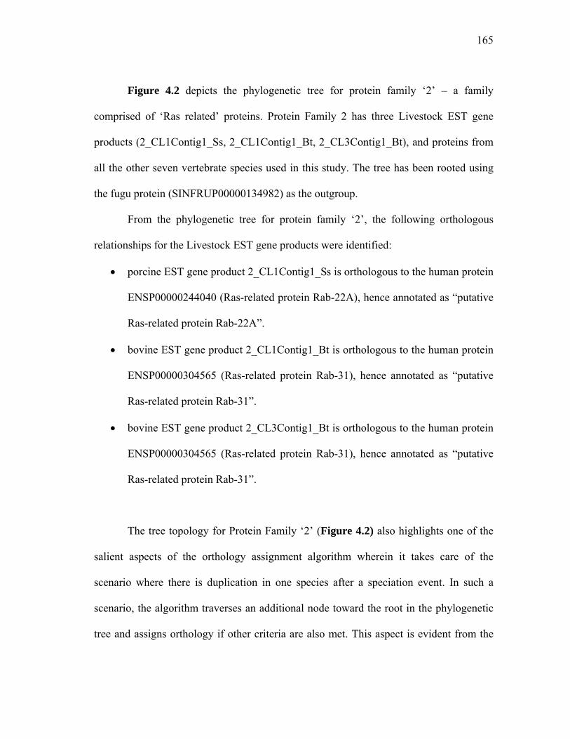
165
Figure 4.2 depicts the phylogenetic tree for protein family ‘2’ – a family
comprised of ‘Ras related’ proteins. Protein Family 2 has three Livestock EST gene
products (2_CL1Contig1_Ss, 2_CL1Contig1_Bt, 2_CL3Contig1_Bt), and proteins from
all the other seven vertebrate species used in this study. The tree has been rooted using
the fugu protein (SINFRUP00000134982) as the outgroup.
From the phylogenetic tree for protein family ‘2’, the following orthologous
relationships for the Livestock EST gene products were identified:
• porcine EST gene product 2_CL1Contig1_Ss is orthologous to the human protein
ENSP00000244040 (Ras-related protein Rab-22A), hence annotated as “putative
Ras-related protein Rab-22A”.
• bovine EST gene product 2_CL1Contig1_Bt is orthologous to the human protein
ENSP00000304565 (Ras-related protein Rab-31), hence annotated as “putative
Ras-related protein Rab-31”.
• bovine EST gene product 2_CL3Contig1_Bt is orthologous to the human protein
ENSP00000304565 (Ras-related protein Rab-31), hence annotated as “putative
Ras-related protein Rab-31”.
The tree topology for Protein Family ‘2’ (Figure 4.2) also highlights one of the
salient aspects of the orthology assignment algorithm wherein it takes care of the
scenario where there is duplication in one species after a speciation event. In such a
scenario, the algorithm traverses an additional node toward the root in the phylogenetic
tree and assigns orthology if other criteria are also met. This aspect is evident from the
166
subtree involving the two bovine EST gene products (2_CL1Contig1_Bt and
2_CL3Contig1_Bt) where there is a duplication event in bovine after speciation; hence
the two bovine EST gene products have been assigned as orthologs to the human protein
ENSP00000304565.
Bovine-porcine one-to-one orthologous combination
Interestingly, 5420 of the 13895 one-to-one orthologous relationships comprised
of a bovine-porcine one-to-one orthologous combination. An example illustrating this is
evident from two of the three orthologous relationships depicted in the phylogenetic tree
for Protein Family ‘15208’ (Figure 4.3). This is a protein family comprised of ‘nuclear
transport factor’ like proteins; it is represented by three Livestock EST gene products
and proteins from six of the other seven vertebrate species used in this study. The tree
has been rooted using the fugu protein (SINFRUP00000135058) as the outgroup. From
the bottom segment of phylogenetic tree for protein family ‘15208’, one can deduce the
bovine-porcine one-to-one orthologous relationship between the bovine EST gene
product 15208_CL1Contig1_Bt and the porcine EST gene product
15208_CL1Contig1_Ss. (Note: The third Livestock EST gene product in this tree,
15208_CL2Contig1_Bt, is involved in a one-to-many orthologous relationship as it is
orthologous to the human proteins ENSP00000339705 and ENSP00000218004.
Annotation transfer in one-to-many orthologous relationships is discussed later in the
text).

167
Figure 4.3: Phylogenetic tree for Protein Family 15208 – a family comprised of ‘nuclear transport factor’ like proteins. The tree is rooted using the fugu protein (SINFRUP00000135058) as the outgroup. Orthology assignments for the three Livestock EST gene products (15208_CL2Contig1_Bt, 15208_CL1Contig1_Ss, 15208_CL1Contig1_Bt) shown in this tree are made as detailed in the text.

168
Annotation transfer – one-to-many orthologous relationships
After identifying putative orthologs for a particular bovine/porcine EST gene
product using the ‘subtree neighbors’ approach, 5880 Livestock EST gene products were
part of different one-to-many orthologous relationships. We had to come up with a
strategy to choose one ortholog, from amongst the many orthologs identified, for
annotation transfer. To do so, we devised a strategy which relies on identifying the
“source” database identifiers from the “Descriptions” of the different Ensembl proteins
identified as putative orthologs. Whenever possible, the ‘Description’ field for a given
Ensembl protein lists the “source” database identifier from which the Ensembl protein
was derived. When information about the database identifier was available, we first
made a note of the source database and we made a choice of which database identifier to
use based on this database order of precedence: UniProtKB [186], RefSeq [187],
Ensembl (when the source identifier was not UniProtKB or RefSeq). We give preference
to UniProtKB for the following reasons:
1. Whenever possible, all the protein products encoded by one gene in a given
species are described within a single UniProtKB entry, including isoforms
generated by alternative splicing, alternative promoter usage, and alternative
translation initiation. In cases where some alternative splicing isoforms derived
from the same gene share only a few exons, the isoforms have to be described in
separate entries [188]. In our dataset, the isoform variants of the different
Ensembl proteins are in the same protein family; hence, there might be instances
169
where an EST gene product involved in a one-to-many orthologous relationship
might actually have the different orthologs mapped to the same UniProtKB entry.
2. UniProtKB is a secondary database, in that it collects information from primary
databases, curates the information if necessary and makes it available.
Information in primary databases (GenBank, GenPept) contain information
submitted by the experimenter and cannot be changed by anybody other the
person who submitted the information. As a result, the primary databases are
essentially archival in nature and cannot correct errors, if any, that are found
later. In other words, annotations from secondary databases like UniProtKB are
more reliable in nature.
For the one-to-many orthologous relationship scenarios, the UniProtKB entry
extracted from the ‘Source’ field of the Ensembl protein is used for annotating the
Livestock EST gene product. Whenever the source database identifier for a given
Ensembl protein was not UniProtKB, we would check to see if the Ensembl protein had
a RefSeq identifier and then we use the Database Mapping tool [189] at UniProtKB to
find the corresponding UniProt entry for the RefSeq identifier. If the RefSeq identifier
did not map to a UniProt entry, we used the RefSeq entry for annotating the Livestock
EST gene product. If we did not find a UniProt or a RefSeq cross-reference for the
Ensembl protein, we ended up using the Ensembl protein itself for annotating the
Livestock EST gene product.

170
The examples below illustrate how the above annotation transfer strategy was
used for Livestock EST gene products involved in one-to-many orthologous
relationships.
Example I: ‘Protein Family 15208’ – nuclear transport factor like proteins
Figure 4.3 depicts the phylogenetic tree for Protein Family ‘15208’, comprised
of ‘nuclear transport factor’ like proteins, and represented by three Livestock EST gene
products and proteins from six of the other seven vertebrate species used in this study.
One of the Livestock EST gene products, 15208_CL2Contig1_Bt, is involved in a one-
to-many orthologous relationship as it is orthologous to the human proteins
ENSP00000339705 and ENSP00000218004, which are isoforms. Table 4.4 lists the
descriptions of these two human proteins.
Table 4.4: Descriptions of Ensembl proteins identified as orthologs for
15208_CL2Contig1_Bt.
Ensembl protein Description
ENSP00000339705 NTF2-related export protein 2. [Source: UniProtKB Q9NPJ8]
ENSP00000218004 NTF2-related export protein 2. [Source: UniProtKB Q9NPJ8]
As evident from Table 4.4, the two isoform variants ENSP00000339705 and
ENSP00000218004 map to the same UniProtKB entry, Q9NPJ8. By the annotation
transfer strategy described above, 15208_CL2Contig1_Bt is annotated as “putative

171
NTF2-related export protein 2” – from the “Description” field of the UniProtKB entry,
Q9NPJ8.
Example II: ‘Protein Family 23614’ – metastatic lymph node (MLN) proteins
Figure 4.4 depicts the phylogenetic tree for Protein Family ‘23614’, comprised
of ‘metastatic lymph node (MLN)’ protein homologs. This protein family is represented
by four Livestock EST gene products and proteins from six of the other seven vertebrate
species used in this study. Two of the Livestock EST gene products,
23614_CL1Contig1_Ss and 23614_29253671_Bt, are involved in a one-to-one bovine-
porcine orthologous relationship. The remaining two Livestock EST gene products,
23614_CL1Contig1_Bt and 23614_CL2Contig1_Ss, are part of one-to-many
orthologous relationships. 23614_CL2Contig1_Ss is involved in a one-to-five
orthologous relationship as it is orthologous to the human protein ENSP00000341409,
the mouse proteins ENSMUSP00000042792 and ENSMUSP00000043328, and the rat
proteins ENSRNOP00000012812 and ENSRNOP00000012820. 23614_CL1Contig1_Bt
is involved in a one-to-six orthologous relationship as it is orthologous to
23614_CL2Contig1_Ss and the five putative orthologs identified for
23614_CL2Contig1_Ss. Table 4.5 lists the descriptions of the five Ensembl proteins
which were identified as orthologs to both 23614_CL1Contig1_Bt and
23614_CL2Contig1_Ss.

172
Figure 4.4: Phylogenetic tree for Protein Family 23614 – a family comprised of ‘metastatic lymph node’ protein homologs. The tree is rooted using the fugu protein (SINFRUP00000176287) as the outgroup. Orthology assignments for the four Livestock EST gene products (23614_CL1Contig1_Ss, 23614_29253671_Bt, 23614_CL1Contig1_Bt, 23614_CL2Contig1_Ss) shown in this tree are made as detailed in the text.
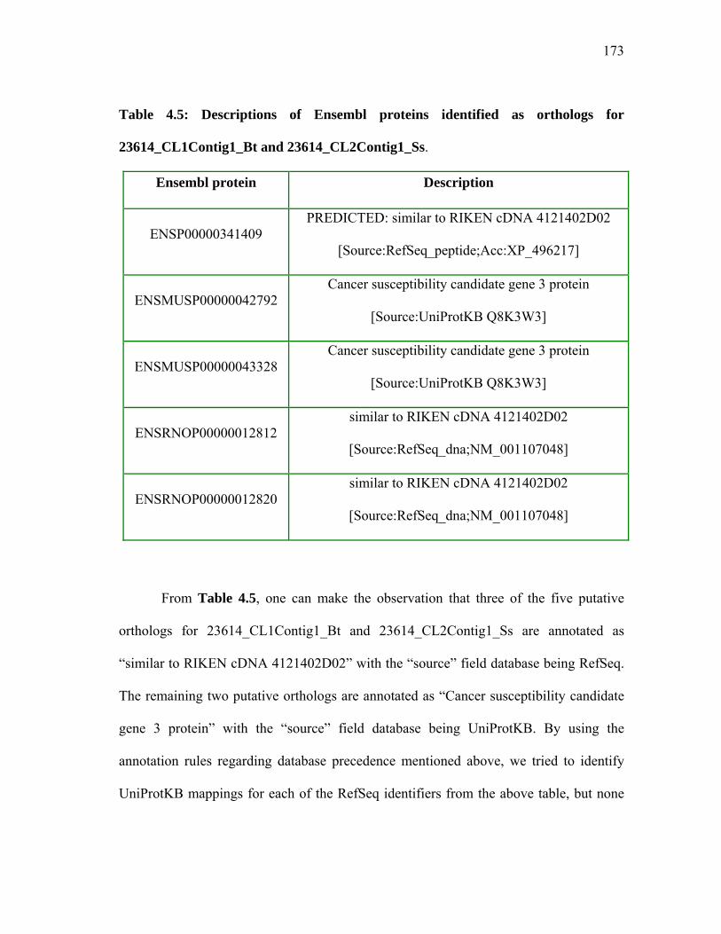
173
Table 4.5: Descriptions of Ensembl proteins identified as orthologs for
23614_CL1Contig1_Bt and 23614_CL2Contig1_Ss.
Ensembl protein Description
ENSP00000341409 PREDICTED: similar to RIKEN cDNA 4121402D02
[Source:RefSeq_peptide;Acc:XP_496217]
ENSMUSP00000042792 Cancer susceptibility candidate gene 3 protein
[Source:UniProtKB Q8K3W3]
ENSMUSP00000043328 Cancer susceptibility candidate gene 3 protein
[Source:UniProtKB Q8K3W3]
ENSRNOP00000012812 similar to RIKEN cDNA 4121402D02
[Source:RefSeq_dna;NM_001107048]
ENSRNOP00000012820 similar to RIKEN cDNA 4121402D02
[Source:RefSeq_dna;NM_001107048]
From Table 4.5, one can make the observation that three of the five putative
orthologs for 23614_CL1Contig1_Bt and 23614_CL2Contig1_Ss are annotated as
“similar to RIKEN cDNA 4121402D02” with the “source” field database being RefSeq.
The remaining two putative orthologs are annotated as “Cancer susceptibility candidate
gene 3 protein” with the “source” field database being UniProtKB. By using the
annotation rules regarding database precedence mentioned above, we tried to identify
UniProtKB mappings for each of the RefSeq identifiers from the above table, but none

174
of the RefSeq identifiers mapped to any UniProtKB entry. Hence, using the annotation
transfer strategy mentioned above, 23614_CL1Contig1_Bt and 23614_CL2Contig1_Ss
were annotated as “putative Cancer susceptibility protein” – from the “Description” field
of the UniProtKB entry, Q8K3W3.
Example III: ‘Protein Family 32278’ – zinc finger proteins
Figure 4.5 depicts the phylogenetic tree for Protein Family ‘32278’, comprised
of ‘zinc finger proteins’. This family is represented by two Livestock EST gene products
and proteins from six of the other seven vertebrate species used in this study. One of the
two Livestock EST gene products, 32278_CL8Contig1_Bt is involved in a one-to-one
orthologous relationship with the human protein ENSP00000262630, which is a “Zinc
finger and BTB domain-containing protein 32”. ENSP00000262630 mapped to the
UniProtKB entry Q9Y2Y4, which had the same description as the Ensembl protein.
Since this is one-to-one orthologous relationship, 32278_CL8Contig1_Bt was annotated
as “similar to human Zinc finger and BTB domain-containing protein 32” using the
“Description” of the UniProtKB entry Q9Y2Y4. The other Livestock EST gene product
in protein family 32278, 32278_CL2Contig1_Ss, is involved in a one-to-five
orthologous relationship as it is orthologous to three human proteins
(ENSP00000346516, ENSP00000352262 and ENSP00000333556), one mouse protein
ENSMUSP00000002095, and one rat protein ENSRNOP00000020573. Table 4.6 lists
the descriptions of the five Ensembl proteins which are identified as orthologs for
32278_CL2Contig1_Ss.

175
Figure 4.5: Phylogenetic tree for Protein Family 32278 – a family comprised of ‘zinc finger’ proteins. The tree is rooted using the fugu protein (SINFRUP00000160592) as the outgroup. Orthology assignments for the two Livestock EST gene products (32278_CL8Contig1_Bt and 32278_CL2Contig1_Ss) shown in this tree are made as detailed in the text.

176
Table 4.6: Descriptions of Ensembl proteins identified as orthologs for
32278_CL2Contig1_Ss.
Ensembl protein Description
ENSP00000346516 Zinc finger protein HRX [Source:UniProtKB Q03164]
ENSP00000352262 Zinc finger protein HRX [Source:UniProtKB Q03164]
ENSP00000333556 Zinc finger protein HRX [Source:UniProtKB Q03164]
ENSMUSP00000002095 Zinc finger protein HRX [Source:UniProtKB P55200]
ENSRNOP00000020573 myeloid/lymphoid or mixed-lineage leukemia
[Source:RefSeq_peptide; NP_001101609]
From Table 4.6, the consensus description for four of the five putative orthologs
is “Zinc finger protein HRX”; each of these four orthologs had UniProtKB as the
“source” field database. The other putative ortholog (ENSRNOP00000020573) had the
description “myeloid/lymphoid or mixed-lineage leukemia” and was sourced from a
RefSeq entry NP_001101609. This RefSeq entry could not be mapped to any
UniProtKB entry. Hence, using the annotation transfer strategy mentioned above,
32278_CL2Contig1_Ss was annotated as “putative Zinc finger protein HRX” – from the
“Description” field of the UniProtKB entry, Q03164.
The annotation transfer strategy for the different one-to-many orthologous
relationship examples discussed above gives precedence to UniProtKB cross-references
of the putative orthologs, where available, for transferring the annotation of one of the
177
putative orthologs to the bovine/porcine EST gene product. This UniProtKB preference
is given irrespective of the number of putative orthologs that had UniProtKB cross-
references. To elaborate, in Table 4.5 (Example II) above, the Livestock EST gene
product, 23614_CL2Contig1_Ss, was part of a one-to-five orthologous relationship. Two
of the five putative orthologs had UniProtKB cross-references and the rest of the
orthologs had RefSeq cross-references. We chose to use the ortholog having a
UniProtKB cross-reference for the transfer of annotation to the Livestock EST gene
product in question. If the putative ortholog does not have a UniProtKB cross-reference,
we give preference to those orthologs that have RefSeq cross-references and if RefSeq
cross-references are not available, one of the Ensembl protein(s) identified as putative
ortholog is used for transfer of annotation.
For the purposes of annotation transfer in one-to-many orthologous scenarios, we
believe that it really should not matter whether on not the putative ortholog had a
UniProtKB or RefSeq cross-reference. We say so because the ‘subtree’ approach used in
our orthology algorithm identifies the distinct subfamily to which a Livestock EST gene
product belongs; since function is conserved within orthologous subfamilies [82], any of
the orthologs in that subfamily can be used for ‘reliable’ annotation transfer. By first
short listing putative orthologs that had UniProtKB cross-references and using them for
annotation transfer, we are only enriching the quality of the annotation for the reasons
discussed earlier.
178
Phylogenomic annotations – can it predict functions for all sequences?
It is well-known that the phylogenomic method cannot predict functions for all
sequences [53], but the predictions that are obtained tend to be accurate; hence, the
annotations can be transferred reliably. In our analysis, we had 86,312 Livestock EST
gene products to begin with, of which only 50,119 sequences passed our multiple
sequence alignment (MSA) editing criteria. From these 50,119 sequences, we were able
to identify predicted functions for only 19,775 Livestock EST gene products at the end
of our phylogenomic annotation pipeline. Sequences get excluded from the
phylogenomic pipeline at the following different stages:
1. Protein families excluded from phylogenetic analysis: we chose to run the
PHYLIP pipeline only on those protein families which have ≤50 sequences in the
edited MSA.
2. Consense step in PHYLIP pipeline: The ‘majority rule extended’ (MRe) method
from the ‘Consense’ step in our PHYLIP pipeline excludes some sequences from
the final tree that did not match its tree resolving criteria.
3. Tree ambiguity in our subtree orthology assignment: If any branch of the
phylogenetic tree contains at least one sequence of the ‘outgroup’ species OR at
least one sequence of the same species as the sequence in question, it denotes
ambiguity in the tree topology pertaining to the sequence in question; hence the
sequence in question is discarded.
179
Currently, there do not exist genomic-scale error-free ‘ortholog gold standard’
datasets [190] and this makes it difficult to analyze and evaluate the performance of the
orthology algorithm. Benchmark datasets like PREFAB [174], BALiBASE [191] and
SABMark [192] are available for evaluation of multiple sequence alignment programs.
Likewise, in the protein structure prediction field, the availability of challenging
benchmark datasets from the Protein Structure Prediction Center [193] in the
international biennial CASP event [194] helps in the assessment of the protein structure
prediction methods. Analogous to the MSA and protein structure prediction benchmark
datasets, the accuracy of phylogenomic methods can be assessed only if rigorously
validated biological data is available [77].
Future work
Future work would include making the phylogeny based function annotations for
bovine/porcine EST gene products accessible from the “Livestock EST Gene Family
Database”. Cattle and pig are more closely related to each other than to the other
vertebrate species used in this study. It would be interesting to know the different cases
in which a protein family has at least one bovine and one porcine EST gene product
where these are not orthologous – using a ‘best hit’ method in this scenario for bovine vs
porcine would have resulted in function prediction and assignment that is not based on
orthology, which would have been erroneous. Comparing the function predictions made
using the ‘best hit’ method with the predictions from the phylogeny based approach
would reveal instances where the ‘best hit’ was not used for function prediction and
180
annotation transfer in the phylogeny based approach. Future work on this front could
address the issue as to why the ‘best hit’ sequence was not the closest neighbor in the
phylogeny based approach.
CONCLUSIONS
In this chapter, we have discussed the development and implementation of a
phylogenomic annotation pipeline to make computational predictions of the functions
encoded in Bos taurus (bovine) and Sus scrofa (porcine) expressed sequence tag (EST)
datasets. As part of the TAMUClust EST clustering pipeline, Bos taurus and Sus scrofa
ESTs were grouped into gene families using the Ensembl vertebrate protein family
clusters. The different EST consensus sequences and proteins in each protein family
were subject to a pipeline involving multiple sequence alignment and phylogenetic tree
construction. This resulted in subdivisions of groups containing orthologs and paralogs,
each group representing distinct subfamilies. Following this, the tree topology was
analyzed and the functions of the uncharacterized EST gene family members were
predicted using a subtree neighbors approach. This approach involves identifying the
subgroup having the sequence (bovine/porcine) whose function is being predicted, and
assigning predicted function based on the most recent diverging sequence from a
different species in that subgroup. Our approach requires estimating a new phylogenetic
tree for each protein family, and the trees need to be recomputed each time a new
sequence is added to the family.

181
For phylogenomic inference to be accurate, all sequences in the set must share
the same domain architecture [68]. In this study, we ensure that this requirement is taken
care of by the clustering algorithm when Ensembl vertebrate proteins are clustered into
protein families. The protein families generated are non-redundant, comprehensive set of
full-length protein clusters with homogeneous domain architecture within clusters and
the pairwise sequence identity between any two proteins within each cluster is at least
55%. Phylogenetic tree construction of these full-length protein clusters with
homogeneous domain architecture enhances the specificity of function annotation for
phylogenomic inference of function [68].
The phylogenomic approach uses phylogenetic trees to determine orthology
between homologs; this requires that the phylogenetic tree topology used as a basis for
inference of function is correct. We address this by performing bootstrap phylogenetic
analysis and obtaining the consensus tree in our PHYLIP pipeline. We use the ‘majority
rule extended’ (MRe) method in the ‘Consense’ step in PHYLIP to obtain the consensus
tree. The MRe method first includes all sequences that appear in more than 50% of the
trees and then considers the other sets of sequences in order of the frequency with which
they have appeared, adding to the consensus tree any sequence compatible with the tree
until the tree is fully resolved. In doing so, the MRe method may exclude some
sequences from the final tree as they did not match the criteria.
We have used the phylogenomic inference method to make computational
predictions of the functions encoded in Bos taurus (bovine) and Sus scrofa (porcine)
expressed sequence tag (EST) datasets. We were able to identify putative functions for
182
~23% of the Livestock EST gene products in our dataset. This, to our knowledge, is the
first time that phylogenomic inference has been used in predicting functions for EST
gene products. The livestock community would largely benefit from the function
predictions of the uncharacterized EST gene family members in cattle and pig from this
analysis. By designing experiments based on these predictions, the number of direct
experiments required to verify function would be drastically reduced.
183
CHAPTER V
SUMMARY
Prediction of functions of genes in a genome is one of the key steps in all
genomic sequencing projects. Sequences that carry out important functions are likely to
be conserved between evolutionarily distant species and cross-species comparisons help
identify these biologically active and conserved regions.
Obtaining insights about the function encoded in an organism by means of
computational function predictions using EST datasets forms the crux of the work in this
dissertation. In this dissertation, the EST clusters from Bos taurus and Sus scrofa EST
datasets were utilized to make computational function predictions. We have shown here
how some of the tools for comparative genomics like sequence homology searching,
annotation transfer, phylogenetic analysis can be used to predict the functions of the
sequence with unknown function.
The TAMUClust method described in this dissertation uses a protein framework
to cluster the ESTs and in doing so, it helps avoid many of the frequently encountered
problems in oligo design - generating oligos with redundant information, and designing
oligos based on chimeric ESTs. The performance of the TAMUClust Bos taurus EST
clusters and the Bos taurus Gene Indices (BTGI) clusters were compared by using
bovine ESTs aligned to the bovine genome assembly as a gold standard. Findings from
the gold standard comparisons reveal that TAMUClust and BTGI are similar in
performance. Comparisons of TAMUClust and TGI with predicted bovine gene models
reveal that both datasets are similar in transcript coverage.

184
The Ensembl protein families from seven vertebrate species were used as a
framework to cluster and assemble the cattle/pig EST datasets, resulting in ‘EST
consensus sequences’ (contigs/singletons) that represent putative genes. These EST
consensus sequences were assigned predicted functions by transferring annotations of
the Ensembl vertebrate protein(s) they get grouped with following sequence homology
searches. The ‘Livestock EST Gene Family Database’ available at
http://genomes.arc.georgetown.edu/cgi-bin/search_livestock_est_gene_family.cgi houses
the annotations. The database has a user-friendly web interface and can be searched in a
number of ways: Cattle/Pig EST GenBank identifiers (GI or accession), Gene Ontology
accession to obtain information about the vertebrate protein family, related EST
members and other annotations. The Livestock EST Gene Family Database is the first of
its kind where ESTs from different species (cattle and pig in this case) are grouped
together in the same gene family. This information comes in handy when a researcher
wants to get a listing of ESTs from different species performing the same function. The
Livestock EST Gene Family Database is also the first of its kind that incorporates a
search strategy that transitively annotates EST gene products with a GO accession and
all its descendants. Searching by GO accession on the Livestock EST Gene Family
Database will retrieve the complete descendant information for the GO accession and
give a mapping of the different cattle and pig EST gene products associated with the
complete GO descendant tree starting from the GO Accession being searched for. This
search feature is useful for researchers wanting to obtain a complete profile of the cattle
and pig EST gene products associated with a particular GO Accession. The Livestock

185
EST Gene Family Database and the annotations housed would help researchers to deal
with the volume of information, and to utilize the information embedded in the gene
expression data gathered from assembling the EST datasets.
Phylogenomic inference of function combines evolutionary and comparative
genomic analysis into a single composite approach, and the function predictions using
this method are more accurate. This approach relies on inferring the function of an
unknown sequence (protein) in the larger context of a protein family based on
evolutionary relationships. Using the phylogenomic method, bovine/porcine EST
consensus sequences belonging to a protein family were grouped with other proteins in
the family, and subject to multiple sequence alignment followed by phylogenetic
analysis. This resulted in subfamilies with each subfamily representing a functionally
and evolutionarily distinct group of sequences with similar functions. By analyzing the
tree topology using a subtree neighbors approach, uncharacterized bovine/porcine EST
gene products were assigned predicted function based on the proteins from the subfamily
in which they got grouped with. To our knowledge, this is the first time that
phylogenomic analysis, and that too on a large scale, has been used in predicting
functions for EST gene products. The annotations for the uncharacterized EST gene
family members in cattle and pig developed using the phylogenomic annotation pipeline
provide the livestock community with a valuable resource to verify function by
designing experiments based on the predictions.
Experimental characterization of sequences, function prediction of sequences and
genomic sequencing can be thought of a three-horse race with the leader being ‘genomic

186
sequencing’ followed by ‘function prediction of sequences’ and ‘experimental
characterization of sequences’ lagging far behind the other two. Computational analysis
of genomes keeps yielding interesting function predictions, even years after the
publication of the sequence; what is most often lacking is systematic experimental
testing of these predictions. In addition, there do not exist genomic-scale error-free
‘ortholog gold standard’ datasets and this makes it difficult to analyze and evaluate the
performance of orthology algorithms. The accuracy of the function prediction methods
can be assessed only if rigorously validated biological data is available, a la, the MSA
and protein structure prediction benchmark datasets that help evaluate the performances
of the multiple sequence alignment and the protein structure prediction methods,
respectively.

187
REFERENCES
1. Eisen JA, Wu M: Phylogenetic analysis and gene functional predictions: phylogenomics in action. Theor Popul Biol 2002, 61(4):481-487.
2. Lockhart DJ, Dong H, Byrne MC, Follettie MT, Gallo MV, Chee MS, Mittmann M, Wang C, Kobayashi M, Horton H: Expression monitoring by hybridization to high-density oligonucleotide arrays. Nature Biotechnology 1996, 14(13):1675-1680.
3. Schena M, Shalon D, Davis RW, Brown PO: Quantitative monitoring of gene expression patterns with a complementary DNA microarray. Science 1995, 270(5235):467-470.
4. Chien CT, Bartel PL, Sternglanz R, Fields S: The two-hybrid system: a method to identify and clone genes for proteins that interact with a protein of interest. Proc Natl Acad Sci U S A 1991, 88(21):9578-9582.
5. Fire A, Xu S, Montgomery MK, Kostas SA, Driver SE, Mello CC: Potent and specific genetic interference by double-stranded RNA in Caenorhabditis elegans. Nature 1998, 391(6669):806-811.
6. Kamath RS, Ahringer J: Genome-wide RNAi screening in Caenorhabditis elegans. Methods 2003, 30(4):313-321.
7. Vidan S, Snyder M: Large-scale mutagenesis: yeast genetics in the genome era. Current Opinion in Biotechnology 2001, 12(1):28-34.
8. Adams MD, Kelley JM, Gocayne JD, Dubnick M, Polymeropoulos MH, Xiao H, Merril CR, Wu A, Olde B, Moreno RF et al: Complementary DNA sequencing: expressed sequence tags and human genome project. Science 1991, 252(5013):1651-1656.
9. Ensembl Genome Browser [http://www.ensembl.org] April 2005.
10. Bovine genome sequencing project at the Baylor College of Medicine [http://www.hgsc.bcm.tmc.edu/projects/bovine/] September 2004.
11. Bovine genome Assemby 3.1 README [ftp://ftp.hgsc.bcm.tmc.edu/pub/data/Btaurus/fasta/Btau20060815-freeze/ReadMeBovine.3.1.txt] August 2006.
188
12. Porcine genome sequencing initiative [http://www.csrees.usda.gov/nea/animals/pdfs/porcine_genome.pdf] April 2005.
13. Pig sequence in Pre-Ensembl [http://pre.ensembl.org/Sus_scrofa/index.html] April 2008.
14. Ureta-Vidal A, Ettwiller L, Birney E: Comparative genomics: genome-wide analysis in metazoan eukaryotes. Nat Rev Genet 2003, 4(4):251-262.
15. Pearson WR, Wood T, Zhang Z, Miller W: Comparison of DNA sequences with protein sequences. Genomics 1997, 46(1):24-36.
16. Dobzhansky T: Nothing in biology makes sense except in the light of evolution. American Biology Teacher 1973, 35(3):125-129.
17. Nobrega MA, Pennacchio LA: Comparative genomic analysis as a tool for biological discovery. J Physiol 2004, 554(Pt 1):31-39.
18. Kimura M: Evolutionary rate at the molecular level. Nature 1968, 217(5129):624-626.
19. King JL, Jukes TH: Non-Darwinian evolution. Science 1969, 164(3881):788-798.
20. Ohta T, Tachida H: Theoretical study of near neutrality. I. Heterozygosity and rate of mutant substitution. Genetics 1990, 126(1):219-229.
21. Eisen JA, Fraser CM: Phylogenomics: intersection of evolution and genomics. Science 2003, 300(5626):1706-1707.
22. Hardison RC: Comparative genomics. PLoS Biol 2003, 1(2):E58.
23. Pennacchio LA, Rubin EM: Genomic strategies to identify mammalian regulatory sequences. Nat Rev Genet 2001, 2(2):100-109.
24. Koonin EV, Galperin MY: Sequence-Evolution-Function: Computational Approaches in Comparative Genomics. Boston: Kluwer Academic Publishers; 2003.
189
25. Aparicio S, Chapman J, Stupka E, Putnam N, Chia J, Dehal P, Christoffels A, Rash S, Hoon S, Smit A: Whole-genome shotgun assembly and analysis of the genome of Fugu rubripes. Science 2002, 297(5585):1301-1310.
26. Frazer KA, Elnitski L, Church DM, Dubchak I, Hardison RC: Cross-species sequence comparisons: a review of methods and available resources. Genome Res 2003, 13(1):1-12.
27. Kent WJ, Zahler AM: Conservation, regulation, synteny, and introns in a large-scale C. briggsae-C. elegans genomic alignment. Genome Res 2000, 10(8):1115-1125.
28. McClelland M, Florea L, Sanderson K, Clifton SW, Parkhill J, Churcher C, Dougan G, Wilson RK, Miller W: Comparison of the Escherichia coli K-12 genome with sampled genomes of a Klebsiella pneumoniae and three Salmonella enterica serovars, Typhimurium, Typhi and Paratyphi. Nucleic Acids Res 2000, 28(24):4974-4986.
29. Fiers W, Contreras R, Duerinck F, Haegeman G, Iserentant D, Merregaert J, Min Jou W, Molemans F, Raeymaekers A, Van den Berghe A: Complete nucleotide sequence of bacteriophage MS2 RNA: primary and secondary structure of the replicase gene. Nature 1976, 260(5551):500-507.
30. Sanger F, Air GM, Barrell BG, Brown NL, Coulson AR, Fiddes CA, Hutchison CA, Slocombe PM, Smith M: Nucleotide sequence of bacteriophage phi X174 DNA. Nature 1977, 265(5596):687-695.
31. Fleischmann RD, Adams MD, White O, Clayton RA, Kirkness EF, Kerlavage AR, Bult CJ, Tomb JF, Dougherty BA, Merrick JM: Whole-genome random sequencing and assembly of Haemophilus influenzae Rd. Science 1995, 269(5223):496-512.
32. Eisen JA: A phylogenomic study of the MutS family of proteins. Nucleic Acids Res 1998, 26(18):4291-4300.
33. Lander ES, Linton LM, Birren B, Nusbaum C, Zody MC, Baldwin J, Devon K, Dewar K, Doyle M, FitzHugh W et al: Initial sequencing and analysis of the human genome. Nature 2001, 409(6822):860-921.
190
34. Venter JC, Adams MD, Myers EW, Li PW, Mural RJ, Sutton GG, Smith HO, Yandell M, Evans CA, Holt RA et al: The sequence of the human genome. Science 2001, 291(5507):1304-1351.
35. Entrez Genome Project [http://www.ncbi.nlm.nih.gov/sites/entrez?db=genomeprj] April 2005.
36. Loots GG, Locksley RM, Blankespoor CM, Wang ZE, Miller W, Rubin EM, Frazer KA: Identification of a coordinate regulator of interleukins 4, 13, and 5 by cross-species sequence comparisons. Science 2000, 288(5463):136-140.
37. Lien CL, McAnally J, Richardson JA, Olson EN: Cardiac-specific activity of an Nkx2–5 enhancer requires an evolutionarily conserved Smad binding site. Developmental Biology 2002, 244(2):257-266.
38. Abrahams BS, Mak GM, Berry ML, Palmquist DL, Saionz JR, Tay A, Tan YH, Brenner S, Simpson EM, Venkatesh B: Novel vertebrate genes and putative regulatory elements identified at kidney disease and NR2E1/fierce loci. Genomics 2002, 80(1):45-53.
39. Sjolander K: Phylogenomic inference of protein molecular function: advances and challenges. Bioinformatics 2004, 20(2):170-179.
40. Galperin MY, Koonin EV: Who's your neighbor? New computational approaches for functional genomics. Nat Biotechnol 2000, 18(6):609-613.
41. Gerlt JA, Babbitt PC: Can sequence determine function? Genome Biol 2000, 1(5):reviews0005.0001 - reviews0005.0010.
42. Altschul SF, Gish W, Miller W, Myers EW, Lipman DJ: Basic local alignment search tool (BLAST). J Mol Biol 1990, 215:403-410.
43. Altschul SF, Madden TL, Schaffer AA, Zhang J, Zhang Z, Miller W, Lipman DJ: Gapped BLAST and PSI-BLAST: a new generation of protein database search programs. Nucleic Acids Res 1997, 25(17):3389-3402.
44. Pearson WR, Lipman DJ: Improved tools for biological sequence comparison. Proc Natl Acad Sci U S A 1988, 85(8):2444-2448.

191
45. Henikoff S, Pietrokovski S, Henikoff JG: Superior performance in protein homology detection with the Blocks Database servers. Nucleic Acids Res 1998, 26(1):309-312.
46. Huynen M, Snel B, Lathe W, 3rd, Bork P: Predicting protein function by genomic context: quantitative evaluation and qualitative inferences. Genome Res 2000, 10(8):1204-1210.
47. Huynen M, Snel B, Lathe W, Bork P: Exploitation of gene context. Curr Opin Struct Biol 2000, 10(3):366-370.
48. Overbeek R, Fonstein M, D'Souza M, Pusch GD, Maltsev N: The use of gene clusters to infer functional coupling. Proc Natl Acad Sci U S A 1999, 96(6):2896-2901.
49. Snel B, Bork P, Huynen M: Genome evolution. Gene fusion versus gene fission. Trends Genet 2000, 16(1):9-11.
50. Karlin S: Detecting anomalous gene clusters and pathogenicity islands in diverse bacterial genomes. Trends Microbiol 2001, 9(7):335-343.
51. Karlin S, Mrazek J: Predicted highly expressed and putative alien genes of Deinococcus radiodurans and implications for resistance to ionizing radiation damage. Proc Natl Acad Sci U S A 2001, 98(9):5240-5245.
52. Karlin S, Mrazek J, Campbell A, Kaiser D: Characterizations of highly expressed genes of four fast-growing bacteria. J Bacteriol 2001, 183(17):5025-5040.
53. Eisen JA: Phylogenomics: improving functional predictions for uncharacterized genes by evolutionary analysis. Genome Res 1998, 8(3):163-167.
54. Bork P, Koonin EV: Predicting functions from protein sequences - where are the bottlenecks? Nat Genet 1998, 18(4):313-318.
55. Doerks T, Bairoch A, Bork P: Protein annotation: detective work for function prediction. Trends Genet 1998, 14(6):248-250.
56. Tomb JF, White O, Kerlavage AR, Clayton RA, Sutton GG, Fleischmann RD, Ketchum KA, Klenk HP, Gill S, Dougherty BA: The complete genome

192
sequence of the gastric pathogen Helicobacter pylori. Nature 1997, 388(6642):539-547.
57. Blattner FR, Plunkett G, III, Bloch CA, Perna NT, Burland V, Riley M, Collado-Vides J, Glasner JD, Rode CK, Mayhew GF et al: The complete genome sequence of Escherichia coli K-12. Science 1997, 277(5331):1453-1462.
58. Tatusov RL, Koonin EV, Lipman DJ: A genomic perspective on protein families. Science 1997, 278(5338):631-637.
59. Xie T, Ding D: Investigating 42 candidate orthologous protein groups by molecular evolutionary analysis on genome scale. Gene 2000, 261(2):305-310.
60. Krishnamurthy N, Brown DP, Kirshner D, Sjolander K: PhyloFacts: an online structural phylogenomic encyclopedia for protein functional and structural classification. Genome Biol 2006, 7(9):R83.
61. Galperin MY, Koonin EV: Sources of systematic error in functional annotation of genomes: domain rearrangement, non-orthologous gene displacement and operon disruption. In Silico Biol 1998, 1(1):55-67.
62. Gerlt JA, Babbitt PC: Divergent evolution of enzymatic function: mechanistically diverse superfamilies and functionally distinct suprafamilies. Annu Rev Biochem 2001, 70:209-246.
63. Doolittle RF: The multiplicity of domains in proteins. Annu Rev Biochem 1995, 64:287-314.
64. Doolittle RF, Bork P: Evolutionarily mobile modules in proteins. Sci Am 1993, 269(4):50-56.
65. Apic G, Gough J, Teichmann SA: Domain combinations in archaeal, eubacterial and eukaryotic proteomes. J Mol Biol 2001, 310(2):311-325.
66. Ekman D, Bjorklund AK, Frey-Skott J, Elofsson A: Multi-domain proteins in the three kingdoms of life: orphan domains and other unassigned regions. J Mol Biol 2005, 348(1):231-243.
67. Basu MK, Carmel L, Rogozin IB, Koonin EV: Evolution of protein domain promiscuity in eukaryotes. Genome Res 2008, 18(3):449-461.

193
68. Krishnamurthy N, Brown D, Sjolander K: FlowerPower: clustering proteins into domain architecture classes for phylogenomic inference of protein function. BMC Evol Biol 2007, 7 (Suppl 1):S12.
69. George DG, Barker WC, Mewes HW, Pfeiffer F, Tsugita A: The PIR-International Protein Sequence Database. Nucleic Acids Res 1996, 24(1):17-20.
70. Fitch WM: Distinguishing homologous from analogous proteins. Syst Zool 1970, 19(2):99-113.
71. Fitch WM: Homology a personal view on some of the problems. Trends Genet 2000, 16(5):227-231.
72. Koonin EV: Orthologs, paralogs, and evolutionary genomics. Annu Rev Genet 2005, 39:309-338.
73. Ohno S: Evolution by gene duplication. New York: Springer-Verlag; 1970.
74. Kondrashov FA, Rogozin IB, Wolf YI, Koonin EV: Selection in the evolution of gene duplications. Genome Biol 2002, 3(2):research0008.0001 - research0008.0009.
75. Lynch M, Conery JS: The evolutionary fate and consequences of duplicate genes. Science 2000, 290(5494):1151-1155.
76. Wagner A: Selection and gene duplication: a view from the genome. Genome Biol 2002, 3(5):reviews1012.
77. Brown D, Sjölander K: Functional classification using phylogenomic inference. PLoS Comput Biol 2006, 2(6):e77.
78. Dayhoff MO, Barker WC, Hunt LT, Schwartz RM: Atlas of protein sequence and structure. Washington, D.C.: National Biochemical Research Foundation; 1978.
79. Thornton J: Gene family phylogenetics: tracing protein evolution on trees. EXS 2002(92):191-207.
80. Thornton JW, DeSalle R: Gene family evolution and homology: genomics meets phylogenetics. Annu Rev Genomics Hum Genet 2000, 1:41-73.
194
81. Eisen JA, Hanawalt PC: A phylogenomic study of DNA repair genes, proteins, and processes. Mutat Res 1999, 435(3):171-213.
82. Eisen JA, Sweder KS, Hanawalt PC: Evolution of the SNF2 family of proteins: subfamilies with distinct sequences and functions. Nucleic Acids Res 1995, 23(14):2715-2723.
83. Henikoff S, Greene EA, Pietrokovski S, Bork P, Attwood TK, Hood L: Gene families: the taxonomy of protein paralogs and chimeras. Science 1997, 278(5338):609-614.
84. Mi H, Lazareva-Ulitsky B, Loo R, Kejariwal A, Vandergriff J, Rabkin S, Guo N, Muruganujan A, Doremieux O, Campbell MJ et al: The PANTHER database of protein families, subfamilies, functions and pathways. Nucleic Acids Res 2005, 33(Database issue):D284-288.
85. Thomas PD, Campbell MJ, Kejariwal A, Mi H, Karlak B, Daverman R, Diemer K, Muruganujan A, Narechania A: PANTHER: a library of protein families and subfamilies indexed by function. Genome Res 2003, 13(9):2129-2141.
86. Haft DH, Loftus BJ, Richardson DL, Yang F, Eisen JA, Paulsen IT, White O: TIGRFAMs: a protein family resource for the functional identification of proteins. Nucleic Acids Res 2001, 29(1):41-43.
87. Finn RD, Tate J, Mistry J, Coggill PC, Sammut SJ, Hotz HR, Ceric G, Forslund K, Eddy SR, Sonnhammer EL et al: The Pfam protein families database. Nucleic Acids Res 2008, 36(Database issue):D281-288.
88. Deluca TF, Wu IH, Pu J, Monaghan T, Peshkin L, Singh S, Wall DP: Roundup: a multi-genome repository of orthologs and evolutionary distances. Bioinformatics 2006, 22(16):2044-2046.
89. Zmasek CM, Eddy SR: ATV: display and manipulation of annotated phylogenetic trees. Bioinformatics 2001, 17(4):383-384.
90. Zmasek CM, Eddy SR: RIO: analyzing proteomes by automated phylogenomics using resampled inference of orthologs. BMC Bioinformatics 2002, 3:14.
195
91. Citerne HL, Luo D, Pennington RT, Coen E, Cronk QC: A phylogenomic investigation of CYCLOIDEA-like TCP genes in the Leguminosae. Plant Physiol 2003, 131(3):1042-1053.
92. Gadelle D, Filee J, Buhler C, Forterre P: Phylogenomics of type II DNA topoisomerases. Bioessays 2003, 25(3):232-242.
93. Daubin V, Gouy M, Perriere G: A phylogenomic approach to bacterial phylogeny: evidence of a core of genes sharing a common history. Genome Res 2002, 12(7):1080-1090.
94. Sicheritz-Ponten T, Andersson SG: A phylogenomic approach to microbial evolution. Nucleic Acids Res 2001, 29(2):545-552.
95. Vienne A, Rasmussen J, Abi-Rached L, Pontarotti P, Gilles A: Systematic phylogenomic evidence of en bloc duplication of the ancestral 8p11.21-8p21.3-like region. Mol Biol Evol 2003, 20(8):1290-1298.
96. Quackenbush J, Cho J, Lee D, Liang F, Holt I, Karamycheva S, Parvizi B, Pertea G, Sultana R, White J: The TIGR Gene Indices: analysis of gene transcript sequences in highly sampled eukaryotic species. Nucleic Acids Res 2001, 29(1):159-164.
97. Mount DW: Bioinformatics: Sequence and Genome Analysis. Cold Spring Harbor: Cold Spring Harbor Laboratory Press; 2004.
98. Adams MD, Dubnick M, Kerlavage AR, Moreno R, Kelley JM, Utterback TR, Nagle JW, Fields C, Venter JC: Sequence identification of 2,375 human brain genes. Nature 1992, 355(6361):632-634.
99. Adams MD, Kerlavage AR, Fleischmann RD, Fuldner RA, Bult CJ, Lee NH, Kirkness EF, Weinstock KG, Gocayne JD, White O et al: Initial assessment of human gene diversity and expression patterns based upon 83 million nucleotides of cDNA sequence. Nature 1995, 377(6547):Suppl pg:3-174.
100. Jongeneel CV: Searching the expressed sequence tag (EST) databases: panning for genes. Brief Bioinform 2000, 1(1):76-92.
101. NCBI dbEST database [http://www.ncbi.nlm.nih.gov/dbEST/] September 2003.

196
102. Boguski MS, Lowe TM, Tolstoshev CM: dbEST - database for "expressed sequence tags". Nat Genet 1993, 4(4):332-333.
103. Parkinson J, Guiliano DB, Blaxter M: Making sense of EST sequences by CLOBBing them. BMC Bioinformatics 2002, 3:31.
104. Ewing R, Poirot O, Claverie JM: Comparative analysis of the Arabidopsis and rice expressed sequence tag (EST) sets. In Silico Biol 1999, 1(4):197-213.
105. Vettore AL, da Silva FR, Kemper EL, Souza GM, da Silva AM, Ferro MI, Henrique-Silva F, Giglioti EA, Lemos MV, Coutinho LL et al: Analysis and functional annotation of an expressed sequence tag collection for tropical crop sugarcane. Genome Res 2003, 13(12):2725-2735.
106. Whitfield CW, Band MR, Bonaldo MF, Kumar CG, Liu L, Pardinas JR, Robertson HM, Soares MB, Robinson GE: Annotated expressed sequence tags and cDNA microarrays for studies of brain and behavior in the honey bee. Genome Res 2002, 12(4):555-566.
107. Parkinson J, Blaxter M: Expressed sequence tags: analysis and annotation. Methods Mol Biol 2004, 270:93-126.
108. EST clustering tutorial [http://bioinf.mpi-inf.mpg.de/conferences/ismb99/WWW/TUTORIALS/tutorial_6.html] April 2005.
109. Quackenbush J, Liang F, Holt I, Pertea G, Upton J: The TIGR Gene Indices: reconstruction and representation of expressed gene sequences. Nucleic Acids Res 2000, 28(1):141-145.
110. UniGene [http://www.ncbi.nlm.nih.gov/sites/entrez?db=unigene] September 2003.
111. Pontius JU, Wagner L, Schuler GD: UniGene: a unified view of the transcriptome. Bethesda: National Center for Biotechnology Information; 2003.
112. Miller RT, Christoffels AG, Gopalakrishnan C, Burke J, Ptitsyn AA, Broveak TR, Hide WA: A comprehensive approach to clustering of expressed human gene sequence: the sequence tag alignment and consensus knowledge base. Genome Res 1999, 9(11):1143-1155.

197
113. The Expressed Gene Anatomy Database (EGAD) [http://www.tigr.org/tdb/egad/egad.shtml] September 2003.
114. Zhang Z, Schwartz S, Wagner L, Miller W: A greedy algorithm for aligning DNA sequences. J Comput Biol 2000, 7(1-2):203-214.
115. EST clustering [http://vit-embnet.unil.ch/CoursEMBnet/Pages02/slides/est_clustering.pdf] April 2005.
116. EST clustering and assembly process at DGI [http://compbio.dfci.harvard.edu/tgi/faq2.html] March 2007.
117. Paracel transcript assembler [www.paracel.com] April 2004.
118. Pevsner J: Bioinformatics and Functional Genomics. Hoboken: Wiley-Liss 2003.
119. Burke J, Davison D, Hide W: d2_cluster: a validated method for clustering EST and full-length cDNAsequences. Genome Res 1999, 9(11):1135-1142.
120. PHRAP [http://www.phrap.com/] September 2003.
121. Burke J, Wang H, Hide W, Davison DB: Alternative gene form discovery and candidate gene selection from gene indexing projects. Genome Res 1998, 8(3):276-290.
122. Doolittle RF, Feng DF, Johnson MS, McClure MA: Relationships of human protein sequences to those of other organisms. Cold Spring Harb Symp Quant Biol 1986, 51 Pt 1:447-455.
123. Pearson WR: Effective protein sequence comparison. Methods Enzymol 1996, 266:227-258.
124. Vasmatzis G, Essand M, Brinkmann U, Lee B, Pastan I: Discovery of three genes specifically expressed in human prostate by expressed sequence tag database analysis. Proc Natl Acad Sci U S A 1998, 95(1):300-304.
125. Wolfsberg TG, Landsman D: A comparison of expressed sequence tags (ESTs) to human genomic sequences. Nucleic Acids Res 1997, 25(8):1626-1632.

198
126. Rudd S: Expressed sequence tags: alternative or complement to whole genome sequences? Trends Plant Sci 2003, 8(7):321-329.
127. The TIGR Gene Indices [http://www.tigr.org/tdb/tgi.shtml] September 2003.
128. The Gene Index Project [http://compbio.dfci.harvard.edu/tgi/] March 2007.
129. Ensembl Release 50 - Bos taurus cDNA [ftp://ftp.ensembl.org/pub/release-50/fasta/bos_taurus/cdna/] July 2008.
130. Gracy J, Argos P: Automated protein sequence database classification. II. Delineation of domain boundaries from sequence similarities. Bioinformatics 1998, 14(2):174-187.
131. Yona G, Linial N, Linial M: ProtoMap: automatic classification of protein sequences, a hierarchy of protein families, and local maps of the protein space. Proteins 1999, 37(3):360-378.
132. Bos taurus Gene Index FTP site [ftp://occams.dfci.harvard.edu/pub/bio/tgi/data/Bos_taurus] March 2007.
133. Bos taurus Gene Index [http://compbio.dfci.harvard.edu/tgi/cgi-bin/tgi/gimain.pl?gudb=cattle] March 2007.
134. Splign [http://www.ncbi.nlm.nih.gov/sutils/splign/splign.cgi] December 2005.
135. GFF3 [http://www.sequenceontology.org/gff3.shtml] January 2006.
136. TGI Clustering tools (TGICL) package [http://compbio.dfci.harvard.edu/tgi/software/] April 2005.
137. Huang X, Madan A: CAP3: A DNA sequence assembly program. Genome Res 1999, 9(9):868-877.
138. Margulies M, Egholm M, Altman WE, Attiya S, Bader JS, Bemben LA, Berka J, Braverman MS, Chen YJ, Chen Z et al: Genome sequencing in microfabricated high-density picolitre reactors. Nature 2005, 437(7057):376-380.

199
139. Rogers YH, Venter JC: Genomics: massively parallel sequencing. Nature 2005, 437(7057):326-327.
140. Goldberg SM, Johnson J, Busam D, Feldblyum T, Ferriera S, Friedman R, Halpern A, Khouri H, Kravitz SA, Lauro FM et al: A Sanger/pyrosequencing hybrid approach for the generation of high-quality draft assemblies of marine microbial genomes. Proc Natl Acad Sci U S A 2006, 103(30):11240-11245.
141. Moore MJ, Dhingra A, Soltis PS, Shaw R, Farmerie WG, Folta KM, Soltis DE: Rapid and accurate pyrosequencing of angiosperm plastid genomes. BMC Plant Biol 2006, 6:17.
142. Wicker T, Schlagenhauf E, Graner A, Close TJ, Keller B, Stein N: 454 sequencing put to the test using the complex genome of barley. BMC Genomics 2006, 7:275.
143. Trombetti GA, Bonnal RJ, Rizzi E, De Bellis G, Milanesi L: Data handling strategies for high throughput pyrosequencers. BMC Bioinformatics 2007, 8 Suppl 1:S22.
144. Matthew E H: Sequencing breakthroughs for genomic ecology and evolutionary biology. Molecular Ecology Resources 2008, 8(1):3-17.
145. Jarvie T, Harkins T: Transcriptome sequencing with the Genome Sequencer FLX system. Nature Methods 2008, 5(9).
146. Bainbridge MN, Warren RL, Hirst M, Romanuik T, Zeng T, Go A, Delaney A, Griffith M, Hickenbotham M, Magrini V et al: Analysis of the prostate cancer cell line LNCaP transcriptome using a sequencing-by-synthesis approach. BMC Genomics 2006, 7:246.
147. Cheung F, Haas BJ, Goldberg SM, May GD, Xiao Y, Town CD: Sequencing Medicago truncatula expressed sequenced tags using 454 Life Sciences technology. BMC Genomics 2006, 7:272.
148. Emrich SJ, Barbazuk WB, Li L, Schnable PS: Gene discovery and annotation using LCM-454 transcriptome sequencing. Genome Res 2007, 17(1):69-73.
200
149. Weber AP, Weber KL, Carr K, Wilkerson C, Ohlrogge JB: Sampling the Arabidopsis transcriptome with massively parallel pyrosequencing. Plant Physiol 2007, 144(1):32-42.
150. Toth AL, Varala K, Newman TC, Miguez FE, Hutchison SK, Willoughby DA, Simons JF, Egholm M, Hunt JH, Hudson ME et al: Wasp gene expression supports an evolutionary link between maternal behavior and eusociality. Science 2007, 318(5849):441-444.
151. Bos taurus (bovine) genome project overview [http://www.ncbi.nlm.nih.gov/sites/entrez?Db=genomeprj&cmd=ShowDetailView&TermToSearch=10708] April 2005.
152. Sus scrofa (pig) genome project overview [http://www.ncbi.nlm.nih.gov/sites/entrez?Db=genomeprj&cmd=ShowDetailView&TermToSearch=10718] April 2005.
153. Vodicka P, Smetana K, Jr., Dvorankova B, Emerick T, Xu YZ, Ourednik J, Ourednik V, Motlik J: The miniature pig as an animal model in biomedical research. Ann N Y Acad Sci 2005, 1049:161-171.
154. Li P, Peatman E, Wang S, Feng J, He C, Baoprasertkul P, Xu P, Kucuktas H, Nandi S, Somridhivej B et al: Towards the ictalurid catfish transcriptome: generation and analysis of 31,215 catfish ESTs. BMC Genomics 2007, 8:177.
155. Stein L: Genome annotation: from sequence to biology. Nat Rev Genet 2001, 2(7):493-503.
156. The Gene Ontology Consortium [http://www.geneontology.org/] September 2004.
157. Ashburner M, Ball CA, Blake JA, Botstein D, Butler H, Cherry JM, Davis AP, Dolinski K, Dwight SS, Eppig JT et al: Gene Ontology: tool for the unification of biology. The Gene Ontology Consortium. Nat Genet 2000, 25(1):25-29.
158. Consortium TGO: Creating the Gene Ontology resource: design and implementation. Genome Res 2001, 11(8):1425-1433.
159. Aho AV, Hopcroft JE, Ullman JD: Data structures and algorithms. Reading: Addison-Wesley 1983.
201
160. Henikoff S, Henikoff JG: Amino acid substitution matrices from protein blocks. Proc Natl Acad Sci U S A 1992, 89(22):10915-10919.
161. Bovine Oligo Microarray Database [http://bovineoligo.org/] May 2006.
162. Swine Protein-Annotated Oligonucleotide Microarray [http://www.pigoligoarray.org/] June 2006.
163. GO Slim and subset guide [http://www.geneontology.org/GO.slims.shtml] September 2006.
164. Stein LD, Mungall C, Shu S, Caudy M, Mangone M, Day A, Nickerson E, Stajich JE, Harris TW, Arva A et al: The generic genome browser: a building block for a model organism system database. Genome Res 2002, 12(10):1599-1610.
165. NCBI PSEG program [ftp://ftp.ncbi.nih.gov/pub/seg/pseg/] April 2005.
166. Wootton JC, Federhen S: Analysis of compositionally biased regions in sequence databases. Methods Enzymol 1996, 266:554-571.
167. BioMart [http://www.biomart.org/] April 2006.
168. Gene Ontology archive [http://archive.geneontology.org/latest/] September 2004.
169. Generic GO Slim [http://www.geneontology.org/GO_slims/goslim_generic.obo] September 2006.
170. AmiGO! Your friend in the Gene Ontology. [http://amigo.geneontology.org/cgi-bin/amigo/go.cgi] September 2005.
171. EXONERATE [http://www.ebi.ac.uk/~guy/exonerate/] October 2006.
172. Slater GS, Birney E: Automated generation of heuristics for biological sequence comparison. BMC Bioinformatics 2005, 6:31.
173. Baldauf SL: Phylogeny for the faint of heart: a tutorial. Trends Genet 2003, 19(6):345-351.
202
174. Edgar RC: MUSCLE: multiple sequence alignment with high accuracy and high throughput. Nucleic Acids Res 2004, 32(5):1792-1797.
175. Notredame C, Higgins DG, Heringa J: T-Coffee: A novel method for fast and accurate multiple sequence alignment. J Mol Biol 2000, 302(1):205-217.
176. Edgar RC: MUSCLE: a multiple sequence alignment method with reduced time and space complexity. BMC Bioinformatics 2004, 5:113.
177. Katoh K, Misawa K, Kuma K, Miyata T: MAFFT: a novel method for rapid multiple sequence alignment based on fast Fourier transform. Nucleic Acids Res 2002, 30(14):3059-3066.
178. T-Coffee user guide [http://envgen.nox.ac.uk/bioinformatics/documentation/T-COFFEE/doc/t_coffee_doc.doc] April 2005.
179. MAFFT user guide [http://align.bmr.kyushu-u.ac.jp/mafft/software/algorithms/algorithms.html#GLE] January 2006.
180. Felsenstein J: 2005. PHYLIP (Phylogeny Inference Package) version 3.6 Distributed by the author. Department of Genome Sciences, University of Washington, Seattle.
181. Stajich JE, Block D, Boulez K, Brenner SE, Chervitz SA, Dagdigian C, Fuellen G, Gilbert JG, Korf I, Lapp H et al: The Bioperl toolkit: Perl modules for the life sciences. Genome Res 2002, 12(10):1611-1618.
182. Jones DT, Taylor WR, Thornton JM: The rapid generation of mutation data matrices from protein sequences. Comput Appl Biosci 1992, 8(3):275-282.
183. Fitch WM, Margoliash E: Construction of phylogenetic trees. Science 1967, 155(760):279-284.
184. Newick tree format [http://evolution.genetics.washington.edu/phylip/newicktree.html] November 2005.
185. Feng DF, Doolittle RF: Progressive sequence alignment as a prerequisite to correct phylogenetic trees. J Mol Evol 1987, 25(4):351-360.
203
186. UniProt Knowledgebase (UniProtKB) [http://www.uniprot.org/] September 2004.
187. NCBI Reference Sequence (RefSeq) [http://www.ncbi.nlm.nih.gov/RefSeq/] September 2004.
188. UniProtKB criteria on isoforms [http://www.uniprot.org/faq/30] April 2008.
189. Database mapping tool at UniProtKB [http://www.uniprot.org/?tab=mapping] April 2008.
190. Chen F, Mackey AJ, Vermunt JK, Roos DS: Assessing performance of orthology detection strategies applied to eukaryotic genomes. PLoS ONE 2007, 2(4):e383.
191. Thompson JD, Plewniak F, Poch O: BAliBASE: a benchmark alignment database for the evaluation of multiple alignment programs. Bioinformatics 1999, 15(1):87-88.
192. Van Walle I, Lasters I, Wyns L: Align-m--a new algorithm for multiple alignment of highly divergent sequences. Bioinformatics 2004, 20(9):1428-1435.
193. Protein Structure Prediction Center [http://predictioncenter.org/index.cgi] June 2002.
194. Moult J, Fidelis K, Rost B, Hubbard T, Tramontano A: Critical assessment of methods of protein structure prediction (CASP) - round 6. Proteins: Structure, Function, and Bioinformatics 2005, 61(S7):3-7.
204
VITA
Name: Anand Venkatraman
Address: Dept. of Biochemistry and Biophysics, Texas A&M University, MS-2128, College Station, TX 77843-2128. Email Address: [email protected] Education: B.Pharmacy, The Tamil Nadu Dr. MGR Medical University, 1997 M.Tech (Biotechnology), Jadavpur University, 1999 Ph.D (Biochemistry), Texas A&M University, 2008