and physics the sensitivity of aerosol in europe to two

Atmos. Chem. Phys., 6, 4287–4309, 2006www.atmos-chem-phys.net/6/4287/2006/© Author(s) 2006. This work is licensedunder a Creative Commons License.

AtmosphericChemistry

and Physics

The sensitivity of aerosol in Europe to two different emissioninventories and temporal distribution of emissions

A. de Meij1, M. Krol 1,*, F. Dentener1, E. Vignati1, C. Cuvelier1, and P. Thunis1

1Institute for Environment and Sustainability, Joint Research Centre, European Commission, Ispra, Italy* now at: SRON, Utrecht, the Netherlands, and Wageningen University, The Netherlands

Received: 7 December 2005 – Published in Atmos. Chem. Phys. Discuss.: 18 April 2006Revised: 11 July 2006 – Accepted: 18 September 2006 – Published: 25 September 2006

Abstract. The sensitivity to two different emission inven-tories, injection altitude and temporal variations of anthro-pogenic emissions in aerosol modelling is studied, using thetwo way nested global transport chemistry model TM5 fo-cussing on Europe in June and December 2000. The simu-lations of gas and aerosol concentrations and aerosol opticaldepth (AOD) with the EMEP and AEROCOM emission in-ventories are compared with EMEP gas and aerosol surfacebased measurements, AERONET sun photometers retrievalsand MODIS satellite data.

For the aerosol precursor gases SO2 and NOx in bothmonths the model results calculated with the EMEP inven-tory agree better (overestimated by a factor 1.3 for both SO2and NOx) with the EMEP measurements than the simulationwith the AEROCOM inventory (overestimated by a factor2.4 and 1.9, respectively).

Besides the differences in total emissions between the twoinventories, an important role is also played by the verticaldistribution of SO2 and NOx emissions in understanding thedifferences between the EMEP and AEROCOM inventories.

In December NOx and SO2 from both simulations agreewithin 50% with observations.

In June SO=4 evaluated with the EMEP emission inventoryagrees slightly better with surface observations than the AE-ROCOM simulation, whereas in December the use of bothinventories results in an underestimate of SO4 with a factor 2.Nitrate aerosol measured in summer is not reliable, howeverin December nitrate aerosol calculations with the EMEP andAEROCOM emissions agree with 30%, and 60%, respec-tively with the filter measurements. Differences are causedby the total emissions and the temporal distribution of theaerosol precursor gases NOx and NH3. Despite these differ-ences, we show that the column integrated AOD is less sensi-tive to the underlying emission inventories. Calculated AOD

Correspondence to:A. de Meij([email protected])

values with both emission inventories underestimate the ob-served AERONET AOD values by 20–30%, whereas a casestudy using MODIS data shows a high spatial agreement.

Our evaluation of the role of temporal distribution of an-thropogenic emissions on aerosol calculations shows that thedaily and weekly temporal distributions of the emissions areonly important for NOx, NH3 and aerosol nitrate. However,for all aerosol species SO=4 , NH+

4 , POM, BC, as well as forAOD, the seasonal temporal variations used in the emissioninventory are important. Our study shows the value of in-cluding at least seasonal information on anthropogenic emis-sions, although from a comparison with a range of measure-ments it is often difficult to firmly identify the superiorityof specific emission inventories, since other modelling un-certainties, e.g. related to transport, aerosol removal, wateruptake, and model resolution, play a dominant role.

1 Introduction

Greenhouse gases and aerosols play an important role inclimate change (Charlson et al., 1991; Kiehl and Briegleb,1993). Greenhouse gases reduce the emission of long waveradiation back to space, leading to a warming of the at-mosphere. Aerosol can change the atmosphere’s radiationbudget by reflecting or absorbing incoming radiation (directeffect) and by modifying cloud properties (indirect effect).Quantification of the role of aerosols on the Earth’s radia-tion balance is more complex than for greenhouse gases, be-cause aerosol mass and particle number concentrations arehighly variable in space and time, and the optical propertiesof aerosol are uncertain.

A good estimate of the emissions of aerosol precursorgases and primary aerosols in the emission inventories istherefore crucial for estimating aerosol impacts on air qualityand climate change, and evaluating coherent reduction strate-gies.

Published by Copernicus GmbH on behalf of the European Geosciences Union.

4288 A. de Meij et al.: Study aerosol with two emission inventories and time factors

Two major uncertainties of the current regional and globalscale emission inventories comprise the accurate estimationof the quantity of the aerosols and precursor emissions, andthe role of the temporal distribution of the emissions in theinventories.

Whereas some work on the impact of the temporal distri-bution of emissions on photochemistry in regional and urbanareas has been performed (e.g. Pont and Fontan, 2001; Pryorand Steyn, 1995; Jenkin et al., 2002), to our knowledge nostudies have been devoted to evaluate its impact on aerosolsurface concentrations and mid-visible aerosol optical depths(AODs). The latter is an important parameter that is neededto calculate the Angstrom parameter, which provides infor-mation on the size of the particles in a given atmosphericcolumn.

This study has two main objectives. The first objective isto evaluate uncertainties in gas, aerosol and aerosol opticaldepth calculations, resulting from two widely used emissioninventories focussing on Europe. To this end we performedwith the global transport chemistry TM5 model simulationsusing a zoom over Europe, for which we had two differ-ent emission inventories available, EMEP and AEROCOM.The European scale EMEP inventory has been used for manyyears in the evaluation of emission reduction strategies, andcontains reported emissions by member countries, as well asexpert estimates. The AEROCOM project provided a com-pilation of recommended global scale aerosol and precursoremission inventories for the year 2000 and was used in therecent AEROCOM global aerosol module intercomparison(Kinne et al., 2006; Textor et al., 2006; Dentener et al., 2006).

The second objective is to evaluate the role of the tempo-ral and height distribution of the emissions on aerosol (pre-cursor) concentrations and AOD calculations. For this weperformed simulations using the EMEP inventory, with thestandard recommendations on the temporal distribution ofemissions (including seasonal variability) and compared it toa simulation ignoring daily emissions variations and anothersimulation that used annual averaged emissions.

The model performance was evaluated comparing aerosolprecursor gases (NOx, SO2, NH3) and aerosols components(SO=

4 , NH+

4 , NO−

3 , black carbon (BC) and particulate or-ganic matter (POM)) to the EMEP network surface observa-tions and to AERONET and MODIS AOD focussing on Juneand December 2000, over Europe.

Section 2 deals with the description of the simulations,model and emission inventories. In Sect. 3 a description ofthe remote sensing data and measurement data is given. InSect. 4 the results are presented. We discuss the results inSect. 5 and we finish with conclusions in Sect. 6.

2 Methodology

Using the two way nested global chemistry transport modelTM5, we performed four simulations for the year 2000. Out-

put was analyzed for a summer (June) and winter (Decem-ber) month to highlight the seasonal dependency of emis-sions and their interaction with the different meteorologicalconditions prevailing in summer and winter.

The first simulation (further denoted as SEMEP) uses theEMEP inventory for the European domain, including theirtemporal (including, daily, weekly and seasonal variability)and height distribution. The second simulation SAERO usedthe AEROCOM recommended emission inventory. The thirdsimulation, SEMEP c, ignored the weekly and daily tempo-ral distribution of emissions, but seasonal temporal distribu-tions are still included. Finally we performed a simulation forwhich a seasonally constant temporal distribution was imple-mented, SEMEP c annual.

2.1 The nested TM5 model

The TM5 model is an off-line global transport chemistrymodel (Bergamaschi et al., 2005; Krol et al., 2005; Peterset al., 2004) driven by meteorological ECMWF (EuropeanCentre for Medium-Range Weather Forecasts) data. Thepresently used configuration of TM5 has a spatial global res-olution of 6◦

×4◦ and a two-way zooming algorithm that al-lows resolving regions, e.g. Europe, Asia, N. America andAfrica, with a finer resolution of 1◦×1◦. A domain of 3◦×2◦

has been added, to smooth the transition between the globaland finer region. The zooming algorithm gives the advantageof a high resolution at measurement locations. The verticalstructure has 25 hybrid sigma-pressure layers. In this studythe 1◦×1◦ resolution was used for Europe/North African re-gion spanning from 21◦ W to 39◦ E and from 12◦ S to 66◦ N.

Transport, chemistry, deposition and emissions are solvedusing the operator splitting. The slopes advection scheme(Russel and Lerner, 1981) has been implemented and deepand shallow cumulus convection is parameterised accordingto Tiedtke (1989).

The gas phase chemistry is calculated using the CBM-IVchemical mechanism (Gery et al., 1989a, b) solved by meansof the EBI (Eulerian Backward Iterative) method (Hertel etal., 1993), like in the parent TM3 model, which has beenwidely used in many global atmospheric chemistry studies(Houweling et al., 1998; Peters et al., 2002; Dentener et al.,2003). In the current model version CO, NMVOC, NH3,SO2 and NOx gas phase, and BC (black or elemental car-bon), POM (particulate organic matter), mineral dust, sea salt(externally mixed), SO=4 , NO−

3 , NH+

4 aerosol componentswere included. Mineral dust and sea salt (SS) were describedusing a log-normal distribution (3 for SS, 2 for dust) andtheir aerosol number and mass were separately transportedusing a fixed standard deviation of the size distribution (Vi-gnati et al., 2005). The aerosol components SO=

4 , methanesulfonic acid (MSA) NO−3 , NH+

4 , POM, and BC, were in-cluded assuming that they were entirely present in the ac-cumulation mode and externally mixed. In this first aerosolversion of TM5, aerosol dynamics (coagulation, nucleation,

Atmos. Chem. Phys., 6, 4287–4309, 2006 www.atmos-chem-phys.net/6/4287/2006/

A. de Meij et al.: Study aerosol with two emission inventories and time factors 4289

condensation and evaporation) are not included. However,gas-aerosol equilibrium of inorganic salts and water up-take is considered using the Equilibrium Simplified AerosolModel (EQSAM version v03d, Metzger, 2000; Metzger etal., 2002a, b). This model allows non-iterative calculationof the equilibrium partitioning of major aerosol compoundsof the ammonia (NH4), nitric acid (NO3), sulphuric acid(SO4) and water system. EQSAM assumes internally mixedaerosols and that the water activity of an aqueous aerosol isequal to the ambientRH (relative humidity). Hence, aerosolwater is a diagnostic rather than transported model parame-ter. Water uptake on SS, is calculated using the descriptionof Gerber et al. (1985).

Formation of secondary organic aerosol was not explicitlydescribed, but included as pseudo organic aerosol emissionsfor the AEROCOM simulation but not for the simulation us-ing EMEP emissions (see Sect. 2.3.2).

Dry deposition is parameterized according to Ganzeveld(1998). In-cloud as well as below-cloud wet removal areparameterized differently for convective and stratiform pre-cipitation, building on the work of Guelle et al. (1998), andJeuken et al. (2001).

For BC and POM we assume 100% hydrophilic propertiesin our model, and hence we assume that BC/POM is removedby wet and dry depositional processes like soluble inorganicaerosol (SO=4 ). TM5 utilized information from the 6-h IPSforecast on 3-D cloud cover and cloud liquid water content,convective and stratiform rainfall rates at the surface, and sur-face heat fluxes to calculated convection.

Removal by convective clouds is taken into account by re-moving aerosols and gases in convective updrafts- with a cor-rection for sub-grid effects on the larger model scale.

Removal by stratiform clouds considers precipitation for-mation and evaporation, and cloud cover, and takes into ac-count a grid-dependency. Effectively rain-out on smallergrids works more effectively than on larger grids. Removalof gases further take their Henry solubility into account. Foraerosol we used an in-cloud wet removal efficiency of 70%for the soluble aerosols and a below cloud removal efficiencyof 100%. Sedimentation was only taken into account for dustand sea salt (large particles) and is considered to be negligi-ble for the sub-micron accumulation mode.

2.2 Aerosol size distribution and AOD calculation

For optical calculations, the accumulation mode aerosol,comprising sulphate, nitrate, ammonium, aerosol water,POM and BC, is described by a fixed Whitby lognormal dis-tribution, using a dry particle median radius of 0.034µm andstandard deviation (σ) 2.0. As mentioned before, dust andsea salt are described with multi-model lognormal distribu-tion. Aerosol mass and number are transported separately,and as a consequence, the size distribution is allowed tochange due to transport and deposition. Two modes are con-sidered for anthropogenic dust (accumulation,σ=1.59 and

coarse,σ=2.0) and three modes for sea salt (Aitken,σ=1.59,accumulation,σ=1.59 and coarse,σ= 2.0). As described be-fore, water uptake by the aerosol is taken into account andmodify the above mentioned diameters.

To calculate aerosol optical depth (AOD) at 550 nm, weuse the Mie code provided by O. Boucher (2004, personalcommunication) to pre-calculate a look-up table for a numberof refractive indices and lognormal distributions. The opticalproperties of these lognormal distributions are determinedby numerical interpolation in discrete size intervals corre-sponding to the median diameter. In Table S1 of the elec-tronic supplement (ES,http://www.atmos-chem-phys.net/6/4287/2006/acp-6-4287-2006-supplement.pdf) the densitiesand optical properties that are used for the optical calcula-tions are listed.

2.3 Emission data

In this study we used two independent emission invento-ries for aerosol and aerosol precursor gases for the year2000. (i) The 50 km×50 km European scale EMEP in-ventory, which is widely used for air quality studies inEurope, and (ii) the 1◦×1◦ global AEROCOM inventory,which is used for climate modelling studies. Below, a briefdescription of the two emission inventories is given, to-gether with the major differences between the two inven-tories. In ES Table S2 (http://www.atmos-chem-phys.net/6/4287/2006/acp-6-4287-2006-supplement.pdf), we presentan overview of the species which are included in the twoemission inventories.

2.3.1 EMEP emission inventory

The Co-operative Programme for Monitoring and Evaluationof the Long-range Transmission of Air Pollutants in Europe(EMEP) evaluates air quality in Europe by operating a mea-surement network, as well as performing model assessments.

The EMEP emission inventory (http://aqm.jrc.it/eurodeltaand http://webdab.emep.int/) contains reported anthro-pogenic emission data for each European country, comple-mented by expert judgements when incomplete or erroneousdata reports are detected. The 50 km×50 km emission in-ventory contains SO2, NOx (as NO2), NH3, NMVOC, CO,PM2.5 and PMcoarse for 11 CORINAIR source sectors. Theemissions are temporally distributed per source sector us-ing time factors. We consider hourly (a multiplication fac-tor that changes each hour and modifies the daily emission),daily (a factor that changes the weekly emissions) and sea-sonally (a factor that changes each month, thus altering theseasonal distribution). For instance, it is important for traf-fic to include rush-hours and weekday-weekend driving pat-terns, and also the intensity of domestic heating differs fromwinter to summer. To match the PM2.5 emissions with thecomponents used in TM5 we assumed the following massfractions: POM 35%, anthropogenic dust 15%, BC 25% and

www.atmos-chem-phys.net/6/4287/2006/ Atmos. Chem. Phys., 6, 4287–4309, 2006

http://www.atmos-chem-phys.net/6/4287/2006/acp-6-4287-2006-supplement.pdf




http://aqm.jrc.it/eurodelta

http://webdab.emep.int/


sulphate 25%, based on Putaud et al. (2003). PM coarse isassumed to contain dust only. We added from the globalAEROCOM emission inventory biomass burning, naturaldust, sea salt and volcanic emissions for the year 2000 (seeSect. 2.3.2). Outside Europe we also use the AEROCOMinventory. ES Table S3 (http://www.atmos-chem-phys.net/6/4287/2006/acp-6-4287-2006-supplement.pdf) provides anoverview of the 11 CORINAIR source sectors, together withthe emissions per sector. Gas and PM emissions are dis-tributed to different height levels based on the sector theybelong to. Point sources and volcanoes are added to theappropriate height, see ES Table S4. Note that unlike forthe AEROCOM inventory, we did not consider pseudo-SOAemissions.

2.3.2 AEROCOM emission inventory

AEROCOM (an AEROsol module inter-COMparison inglobal models, seehttp://nansen.ipsl.jussieu.fr/AEROCOM)evaluates aerosol concentrations, optical properties, and re-moval processes in 21 global models (Kinne et al., 2006;Textor et al., 2006). AEROCOM experiment B aims at con-straining the models by providing a prescribed set of globalnatural and anthropogenic emissions for the year 2000. Webriefly call this ad-hoc compilation of the best inventoriesthat was available in the year 2003 the AEROCOM inven-tory, ftp://ftp.ei.jrc.it/pub/Aerocom(Dentener et al., 2006).

Monthly varying large scale biomass burning emissions ofPOM, BC and SO2 are based on GFED 2000 (Global FireEmissions Database) (Van der Werf et al., 2003). Globalemissions amount to 34.7 Tg, 3.06 Tg and 4.11 Tg (SO2),respectively. Fossil fuel/bio fuel related POM (12.3 TgPOM/yr) and BC (4.6 Tg C/year) emissions are based onBond et al. (2004). Country and region based SO2 emis-sions for the year 2000 are provided by IIASA (Denteneret al., 2006; Cofala et al., 2005) and geographically dis-tributed with the EDGAR3.2 1995 data base. Global emis-sions amount to 138.3 Tg SO2/year and 3.5 Tg SO4/year.Natural emissions of SO2 (e.g. volcanoes) are an update ofthe GEIA recommended datasets.

Daily averaged DMS emissions were taken from theLMDZ model (O. Boucher, 2003, personal communication)using the DMS surface water concentrations of Kettle andAndreae (2000) and the horizontal wind speed (Nightingaleet al., 2000). Yearly DMS amount to 20.8 TgS. Daily sea saltemissions were taken from Gong (2002, 2003a, b), interpo-lated to a three modal distribution with a cut-off at r=10µm,resulting in 8356 Tg/year. Similarly, daily dust emissions for2000 are based on Ginoux (2004), were interpolated to 2 log-normal modes, corresponding to a global total of 1681 Tg/yr.

Secondary organic aerosol is an important componentof the aerosol system (Kanakidou et al., 2005). Sincemost AEROCOM models did not include a description ofthe formation of SOA (Secondary Organic Aerosol), andthere are major difficulties to describe the formation pro-

cesses of SOA, AEROCOM therefore made the simpli-fying assumption that 15% of natural terpene emissionsform SOA, altogether amounting to 19.11 Tg POM/year. Inthe TM5 model most other anthropogenic emissions suchas NOx are taken from the EDGAR3.2 (1995) database,http://www.mnp.nl/edgar. NH3 emissions were based onBouwman et al. (1997, 2002), and distributed using thehours of daylight per month after Dentener and Crutzen(1994). For the other components the yearly emissionsare equally distributed over the year with no seasonal vari-ations. ES Table S5 (http://www.atmos-chem-phys.net/6/4287/2006/acp-6-4287-2006-supplement.pdf) includes theheight of the emissions which are applied in the AEROCOMemission inventory.

2.3.3 EMEP emission inventory versus AEROCOM emis-sion inventory

There are substantial differences between the two emissioninventories in describing BC, dust, POM, and sulphate emis-sions. The EMEP inventory contains detailed country basedknowledge on a 50×50 km resolution, while the AEROCOMinventory offers the advantage of global consistency. EMEPreports PM2.5 emissions, which were disaggregated by usinto individual aerosol components. For example, we as-sume that 25% and 35% of the PM2.5 emissions consists ofBC and POM, while the AEROCOM BC and POM emis-sions are based on a technology based global inventory ofblack carbon emissions from fossil fuel and bio-fuel com-bustion (Bond et al., 2004). 15% of the EMEP PM2.5 isassumed to be anthropogenic dust (e.g. vehicular movementscausing re-suspension of particles), while AEROCOM con-tains only natural dust emissions (Ginoux et al., 2004). Par-ticularly relevant for this study are the emissions from theSahara. Finally, we assume that the remaining 25% of theEMEP PM2.5 emissions is primary sulphate. In the AERO-COM simulation we assume that 2.5% of all SOx of the AE-ROCOM emissions is emitted as primary sulphate. Thesedifferent procedures result for the European domain in dif-ferent primary sulphate emissions of 0.22 and 0.23 Tg/year,respectively.

Focussing on the European domain, we give in ESTable S6 (http://www.atmos-chem-phys.net/6/4287/2006/acp-6-4287-2006-supplement.pdf) an overview of the result-ing total emissions of NOx, CO, SO2, NH3, SO4, sea salt,BC, POM and dust included in the two inventories for Eu-rope in June, December and the annual amount.

The annual emissions of the two inventories are generallywithin 20%, however the annual AEROCOM POM emis-sions are higher by 45%, NH3 by 37% and mineral dust by34%. The difference between the European scale NH3 AE-ROCOM (6.0 Tg) and EMEP (4.4 Tg) emissions stems likelyfrom the recent NH3 emission abatement measures to combateutrophication problems in Northern Europe. These are in-cluded in the EMEP, but not in the Bouwman et al. (2002) in-




http://nansen.ipsl.jussieu.fr/AEROCOM

ftp://ftp.ei.jrc.it/pub/Aerocom

http://www.mnp.nl/edgar






ventory. The much larger POM emissions in the AEROCOMinventory are due to the presence of SOA pseudo-emissions,which were not included in the EMEP emission inventory.

The differences in dust emissions are only due to the an-thropogenic dust sources from agriculture and transport in-cluded in the EMEP inventory. These emissions are addedto the natural mineral dust from AEROCOM which was in-cluded in both inventories.

Larger differences appear in June, where we see that AE-ROCOM emissions of NOx, SO2, SO4, NH3, and POM arehigher by 39%, 18%, 31%, 67% and 248%, respectively. Ex-cept for POM, these differences are mainly due to the sea-sonal time factors which are applied to the EMEP inventoryonly.

For December (ES Table S6, http://www.atmos-chem-phys.net/6/4287/2006/acp-6-4287-2006-supplement.pdf) the above mentioneddiscrepancies are smaller than in June, due to compen-sating effect of the seasonal distribution and the yearlydiscrepancies of the two inventories.

3 Description measurement data sets

For evaluation of the computed gas and aerosol concentra-tions we compare with EMEP measurements of SO2, NOx,and aerosol components. Model calculated AOD is com-pared with sun photometer data from the AERONET stationslocated in Europe, and MODIS (Moderate Resolution Imag-ing Spectro radiometer) satellite data.

The EMEP air quality monitoring network measures sincethe late 1970s ozone, heavy metals, Persistent Organic Pollu-tants (POPs), Volatile Organic Compounds (VOC) and par-ticulate matter (PM2.5, PM10, SO=4 , NO−

3 and NH+)4 at

ca. 150 sites in Europe. The aerosols are measured with adaily time resolution; SO2 and NOx are reported hourly. Notevery station measures all components, therefore the num-ber of EMEP stations available for comparison with modelresults differs per component.

One of the artefacts occurring with the main filter type(quartz) used by most EMEP stations is the evaporationof ammonium nitrate at higher temperatures. Tempera-tures exceeding 20◦C cause complete NH4NO3 evapora-tion from the quartz filter, a loss of 100%; and a loss ofabout 25% for NH+4 , based on 5–10µg/m3 NO−

3 and 10–20µg/m3 SO=

4 at Ispra during a summer month (ratio 2:1 for(NH4)2SO4/NH4NO3).

Temperatures between 20 and 25◦C cloud lead to a loss of50% of the nitrate aerosol (Schaap et al., 2003a, b). There-fore almost all reported summer NH4NO3 and NH+

4 concen-trations present only a lower limit, rather than a realistic con-centration.

The AERONET (AErosol RObotic NETwork) Cimel sunphotometers (Holben et al., 1998) used in this study are givenin ES Table S7 (http://www.atmos-chem-phys.net/6/4287/

2006/acp-6-4287-2006-supplement.pdf). Due to cloudinessnot all days of June and December could be used for aerosolretrieval. The sun photometer measures (every 15 min) ina 1.2◦ field of view, at eight solar spectral bands (340, 380,440, 500, 670, 870, 940 and 1020 nm). These solar extinctionmeasurements are used to calculate for each wavelength theaerosol optical depth, with an accuracy of±0.01–0.02 (Ecket al., 1999). Sun photometer acquires aerosol data only dur-ing daylight and in cloud free conditions. In this work thecloud screened and quality-assured level 2 data are used.

We used AOD at 550 nm, calculated from the AOD val-ues reported at 870 and 440 nm, using the information onthe Angstrom coefficient (S. Kinne, personal communica-tion, 2004).

The MODIS (Moderate Resolution Imaging Spectro ra-diometer) on board of NASA’s Terra Earth Observing Sys-tem (EOS) mission retrieves aerosol over land (Kaufman etal., 1997) and ocean (Tanre et al., 1997) at high resolution.MODIS has one NADIR looking camera which retrievesdata in 36 spectral bands, from 0.4µm—14.5µm with spa-tial resolutions of 250 m (bands 1–2), 500 m (bands 3–7)and 1000 m (bands 8–36). Daily level 2 (MOD04) aerosoloptical thickness data are produced at the spatial resolu-tion of 10×10 km over land, aggregated from the original1 km×1 km pixel size. As the swath width is about 2330 km,the instrument has almost a daily global coverage. Uncer-tainties in the MODIS products over land are relatively large.High albedo areas like the Sahara Desert and snow/ice cov-ered regions and complex terrain are difficult for the MODISinstrument, leading to a large bias with models and groundbased observations (Chin et al., 2004). Reported MODISaerosol errors are1τa=±0.05±0.15τa (Remer et al., 2005).Level 2 cloud screened, version 003 files are used for thiswork. We present in Sect. 4 a case study for the 11 June2000.

4 Results

In this section we present first an evaluation of the im-pact of using the EMEP and AEROCOM inventories (SEMEPand SAERO) and compare them with EMEP measurements(Sect. 4.1). In Sect. 4.2 we subsequently demonstrate thespatial variability of AOD associated with using these twoemissions inventories, and compare it to MODIS retrievals.In Sect. 4.3 we assess the temporal variability of AOD bycomparing to AERONET sun photometer data. Finally inSect. 4.4, we perform two sensitivity studies to analyse theimpact of daily, weekly and seasonal temporal distributionof emissions on gas, aerosol and AOD calculations. For theinterested reader, detailed station information and statisticsper component are presented in the accompanied electronicsupplement to this paper.








(a)

Mean SO2 EMEP JUNE

0.0 0.2 0.4 0.7 0.9 1.1 1.3 1.6 1.8 2.0 ppb

Correlation stations: 0.83 / Best fit: y = 1.31x

0 1 2 3Measured mean concentration

0

1

2

3

Mod

eled

mea

n co

ncen

trat

ion

FI37 GB06

GB13

GB16

IT04

NL10

NO01 NO08

SE08

(b)

Mean SO2 AEROCOM JUNE

0.0 0.2 0.4 0.7 0.9 1.1 1.3 1.6 1.8 2.0 ppb


0 1 2 3Measured mean concentration

0

1

2

3

Mod

eled

mea

n co

ncen

trat

ion

FI37 GB06

GB13

GB16

IT04

NL10

NO01

NO08

SE08

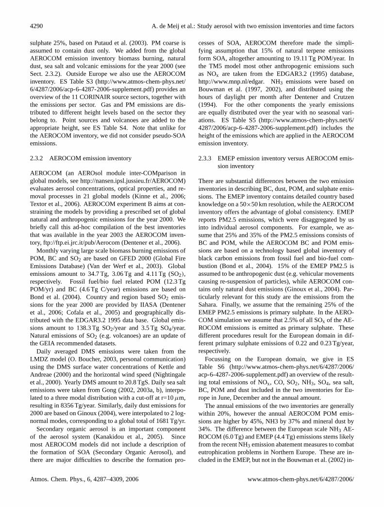
Fig. 1. (a), (b), (c) and(d) are presenting the monthly average measured mixing ratio (inner circle) of SO2 and calculated (outer circle) SO2by SEMEP and SAERO for June and December 2000. For reference, the 2:1 and 1:2 lines are shown as the dashed lines, the 1:1 line as solidand the line of best fit is red solid.

4.1 Evaluation of SEMEP and SAERO with surface observa-tions

In order to compare EMEP station data with model resultson a 1◦×1◦ grid, we selected those measurement stationsable to represent the model spatial scale and which had suffi-ciently data completeness for the month under consideration.First we compare daily average concentrations modelled atthe EMEP stations to the measurement data. If the temporalcorrelation between the time series (with a data complete-ness of at least 10 days/month) is less than 0.5 (either inSEMEP and SAERO), due to measurement errors and sparsedata availability, we excluded the stations from the analysis.An other possible reason for bad correlation between modeland measurements, is that apparently the sub-grid scale localmeteorology can not be accurately described by the resolu-tion (1◦

×1◦) of the model.

This procedure allows a fair comparison between mea-sured and modelled concentrations. Subsequently we de-

termined the spatial correlation using the monthly averagedconcentration, and calculate the model bias.

We evaluate the sulphate and nitrate aerosol precursorgases SO2, and NOx, and the aerosol components SO=

4 ,NO−

3 , NH+

4 and BC. The overall evaluation is presented inFigs. 1, 2 and 3, which shows the monthly mean concentra-tion distribution over Europe.

4.1.1 SO2

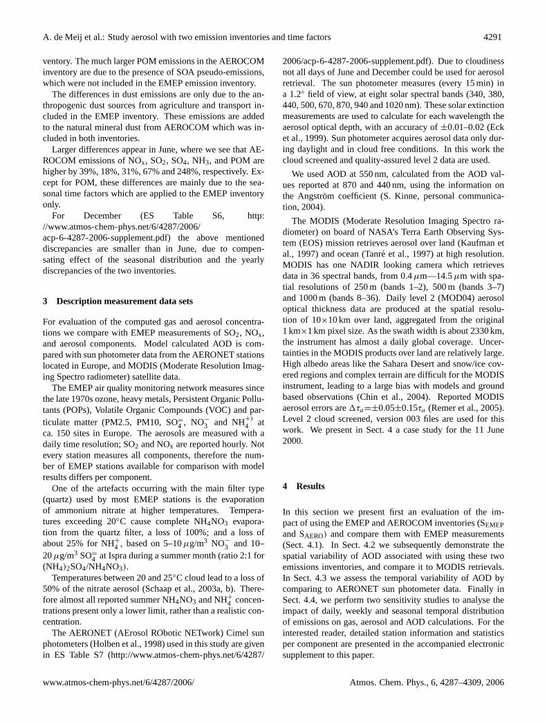
In Figs. 1a–d we present an evaluation of SEMEP andSAERO computed SO2 concentrations. In June, both sim-ulations show high spatial correlation coefficients, of 0.83and 0.92, respectively (based on 9 stations, 68 station re-jected). The June mean SO2 concentrations for SEMEP arein better agreement (an overestimate of 31%) with the mea-sured values than SAERO (an overestimate by a factor 2.4).This discrepancy can not be explained by differences in theemissions alone, since the AEROCOM emissions of SO2are only 18% higher over Europe than the EMEP inven-



(c)

Mean SO2 EMEP DEC

0.0 1.1 2.2 3.3 4.4 5.6 6.7 7.8 8.9 10.0 ppb


0 2 4 6 8 10Measured mean concentration

0

2

4

6

8

10

Mod

eled

mea

n co

ncen

trat

ion

AT02

DK03 FI17 FI37 GB06

GB13 GB15

NL10

PL02

PL05

SE08

YU05

(d)

Mean SO2 AEROCOM DEC

0.0 1.1 2.2 3.3 4.4 5.6 6.7 7.8 8.9 10.0 ppb


0 2 4 6 8 10Measured mean concentration

0

2

4

6

8

10

Mod

eled

mea

n co

ncen

trat

ion

AT02

DK03 FI17 FI37 GB06

GB13 GB15

NL10

PL02

PL05

SE08

YU05

Fig. 1. Continued.

tory (ES Table S6,http://www.atmos-chem-phys.net/6/4287/2006/acp-6-4287-2006-supplement.pdf). A likely explana-tion lies in the vertical distribution of the emissions appliedin the inventories (ES Tables S4 and S5). For that reason wepresent in Figs. 2a and b the June mean SO2 surface con-centrations. Especially in the eastern part of Europe the SO2concentrations by SAERO at ground level are up to a factor of2 higher due to the higher fraction of emissions in the low-est model layer. When we compare the SO2 distributions at950 hPa (±500 m, Figa. 2c and d) we observe especially inEastern Europe an opposite situation; smaller SO2 emissionsfrom domestic heating (contributing by 6.8% to all emis-sions). In SAERO SO2 is emitted at ground level only, whichcould be held responsible for the higher SO2 concentrationsat ground level, where in EMEP 50% of SO2 is emitted at ahigher level.

For December the difference between the SO2 calculationsby SEMEP and SAERO is much smaller, see Figs. 1c and d(based on 12 stations used and 66 rejected). On a monthlyaveraged basis SEMEP concentrations are 2% lower than themeasurements, with a spatial correlation coefficient of 0.91.

SAERO overestimates the measurements with 47% and has ahigh spatial correlation of 0.94. Note that the high corre-lation coefficients are statistically not robust (Figs. 1c andd), since they are determined by a few stations with a highspread in the monthly mean concentrations. The better agree-ment for the two simulations in December is in line with thesmaller differences (2%) between the two emission inven-tories (see ES Table S6,http://www.atmos-chem-phys.net/6/4287/2006/acp-6-4287-2006-supplement.pdf). Tables S9aand S9b of the electronic supplement contain for each stationthe calculated monthly mean and correlation coefficients forSEMEP and SAERO together with the measured monthly meanand the number of measurements for June and December.

4.1.2 NOx

In June, SEMEP slightly overestimates (by 28%) the monthlymean NOx values, while the SAERO simulation overes-timates NOx by a factor of 1.95 (not shown). Spa-tial correlation coefficients are 0.79 and 0.53, respec-tively (based on 11 stations, 49 rejected). The difference







(a) (b)

(c) (d)

Fig. 2. Monthly SO2 distribution by SEMEP and the SAERO at surface level (a andb, respectively) and 950 hPa (c andd, respectively) forJune 2000.

can be partly explained by the overall higher (39%, ESTable S6, http://www.atmos-chem-phys.net/6/4287/2006/acp-6-4287-2006-supplement.pdf) monthly emissions in theAEROCOM inventory compared to EMEP. However, thestations available for comparison with measurements seemheavily biased to Northern Europe, where indeed the spa-tial difference between the EMEP and AEROCOM inventoryseems higher. The vertical distribution plays also here an im-portant role. The monthly mean NOx surface concentrationsby SAERO are up to a factor of 2 higher in the Northern partof Europe, due to higher emissions in the lowest model layer(not shown). The differences in monthly mean NOx concen-trations at±500 m between SAERO and SEMEP are smaller.

In December, SEMEP and SAERO NOx mean con-centrations are closer to the measurements, andare respectively 7% and 11% higher (see ES Ta-ble S10b, http://www.atmos-chem-phys.net/6/4287/2006/acp-6-4287-2006-supplement.pdf). Spatial correlations are0.76 and 0.79 for SEMEP and SAERO, respectively (based on17 stations, 43 rejected).

4.1.3 SO=

4

Figures 3a–d present the EMEP measured and modelled(SEMEP and SAERO) SO=

4 concentrations for June and De-cember 2000. Spatial correlation coefficients are compara-ble for SEMEP (0.66) and SAERO (0.65) (based on 38 stations







(a)

Mean SO4 EMEP JUNE

0.0 0.2 0.4 0.7 0.9 1.1 1.3 1.6 1.8 2.0 ppb


0.0 0.5 1.0 1.5 2.0Measured mean concentration

0.0

0.5

1.0

1.5

2.0

Mod

eled

mea

n co

ncen

trat

ion

AT02

CH05 ES04

ES11

FI09 FI17 FI37

FR05 FR09 FR10

FR13

GB02

GB04

GB06

GB07

GB13 GB14

GB15 GB16

HU02

IE03 IE04 LT15 NL09

NL10

NO01 NO08

NO39

NO41

PL02

PL04 PL05

RU16

RU18

SE02

SK04 SK05

TR01

(b)

Mean SO4 AEROCOM JUNE

0.0 0.2 0.4 0.7 0.9 1.1 1.3 1.6 1.8 2.0 ppb



0.0

0.5

1.0

1.5

2.0

Mod

eled

mea

n co

ncen

trat

ion

AT02

CH05

ES04

ES11

FI09

FI17

FI37

FR05 FR09 FR10

FR13

GB02

GB04

GB06

GB07

GB13 GB14

GB15 GB16

HU02

IE03

IE04

LT15 NL09

NL10

NO01 NO08

NO39

NO41

PL02

PL04 PL05

RU16

RU18

SE02

SK04 SK05

TR01

Fig. 3. (a), (b), (c) and(d) are presenting the monthly average measured mixing ratio (inner circle) of SO=4 and calculated (outer circle)

SO=4 by SEMEP and SAERO for June and December 2000. For reference, the 2:1 and 1:2 lines are shown as the dashed lines, the 1:1 line as

solid and the line of best fit is red solid.

used and 33 rejected). The modelled SO=

4 concentrationsby SEMEP match the measurements while SAERO on averageslightly overestimates SO=4 aerosol concentrations by 19%.Especially over central Europe (Austria, Hungary, CzechRepublic and Poland) significantly higher SO=

4 concentra-tions are calculated by SAERO than for SEMEP, which canbe attributed to the higher over-all emissions. For Decem-ber the differences between the two simulations are rathersmall and both SEMEP and SAERO underestimate on av-erage the modelled SO=4 aerosol concentrations comparedwith measurement data by as much as a factor 2 (basedon 23 stations, 45 rejected). The wintertime underestima-tion of sulphate concentrations has been observed earlierand is possibly due to a lack of oxidation chemistry in themodel (Jeuken, 2000; Kasibhatla et al., 1997). More de-tailed information in Tables S11a and S11b of the electronicsupplement (http://www.atmos-chem-phys.net/6/4287/2006/acp-6-4287-2006-supplement.pdf).

4.1.4 NO−

3

Since in summer EMEP measurements have serious mea-surement artefacts (see Sect. 3) we can only analyse dif-ferences between nitrate aerosol computed by SEMEP andSAERO for December. Substantial differences are found forNO−

3 aerosol: SAERO calculates a maximum concentrationof 22.1µg/m3 over Germany, while the SEMEP calculatedmaximum amounts to 9.6µg/m3. Over Poland SAERO cal-culates NO−3 aerosol values of 5µg/m3, while SEMEP calcu-lates NO−

3 aerosol<2µg/m3. The higher NO−3 found withthe AEROCOM inventory, can be understood from higherNOx (+39%) and NH3 (+67%) emissions in the AEROCOM(taken from EDGAR3.2 database) than in the EMEP inven-tory.

Reactions (1–4) show how NO−3 aerosol formation is re-lated to both NOx and NH3 emissions:

NO2(g) + OH(g) + M → HNO3(g) + M (R1)





(c)

Mean SO4 EMEP DEC

0.0 0.1 0.2 0.3 0.4 0.6 0.7 0.8 0.9 1.0 ppb



0.0

0.5

1.0

1.5

2.0

Mod

eled

mea

n co

ncen

trat

ion

PL05

CH02

ES04 ES09 ES12 ES13 ES15

FR03 FR05

FR09

FR10

FR13 GB07

GB13 GB14 GB15

HU02 IT01

LT15

NL10

NO08

PL02

PL04

(d)

Mean SO4 AEROCOM DEC

0.0 0.1 0.2 0.3 0.4 0.6 0.7 0.8 0.9 1.0 ppb



0.0

0.5

1.0

1.5

2.0

Mod

eled

mea

n co

ncen

trat

ion

PL05

CH02

ES04 ES09 ES12 ES13 ES15 FR03 FR05

FR09

FR10

FR13

GB07

GB13 GB14

GB15

HU02

IT01

LT15

NL10

NO08

PL02

PL04

Fig. 3. Continued.

and,

NO2(g) + NO3(g) → N2O5 (R2)

The hydrolysis of N2O5 on wet aerosol surfaces is an im-portant pathway to convert NOx into HNO3 (Dentener andCrutzen, 1993; Riemer et al., 2003; Schaap et al., 2003a, b):

N2O5(g) + H2O → 2HNO3 (R3)

NH3(g) + HNO3(g) ↔ NH4NO3(aq,s) (R4)

For December SEMEP overestimates measured aerosol nitrateby a factor of 1.37, and SAERO by a factor of 1.62. Ta-ble S12 in the ES (http://www.atmos-chem-phys.net/6/4287/2006/acp-6-4287-2006-supplement.pdf) shows that SAEROaerosol nitrate concentrations are at all stations higher thanthose of SEMEP (except for PL02). A possible explanationfor these differences could be related to higher NH3 emis-sions (21% higher in winter) in the AEROCOM than in theEMEP inventory. High spatial correlation coefficients of 0.84(EMEP) and 0.91 (AEROCOM) are found (based on 6 sta-tions, 15 rejected), indicating that the spatial gradients of the

monthly mean concentrations are relatively well reproducedby the model.

4.1.5 NH+

4

EMEP reports in many cases the sum of NH3 and NH+

4 , alsocalled total ammonium (NHx). For these cases we comparedmeasurements to the modelled sum of the two components.

SEMEP NHx concentrations agree well with measurementsfor June, and are on average only 4% higher. In con-trast, SAERO overestimates NHx on average by a factorof 2.0. Analyzing the monthly mean concentrations (ESTable S13a,http://www.atmos-chem-phys.net/6/4287/2006/acp-6-4287-2006-supplement.pdf), we see that for all sta-tions the values are higher for SAERO than for SEMEP (basedon 20 stations, 17 rejected). The overestimation of SAEROcan explained by the 67% higher summer NH3 emissionscompared to the EMEP emission inventory. The spatial cor-relation coefficients are high with 0.81 and 0.80, respectively.

For December SAERO agrees better with the measure-ments, and on average SAERO and SEMEP underestimate the







Table 1. Monthly mean BC and POM concentrations (µg/m3) for all the stations calculated by SEMEP and SAERO, together with EMEPmeasurement data for December 2002 and June 2003.

BCEMEP 2002 Decµg/m3

SEMEP 2000 Decµg/m3

SAERO 2000 Decµg/m3

EMEP 2003 Juneµg/m3

SEMEP 2000 Juneµg/m3

SAERO 2000 Juneµg/m3

Average 1.25 0.47 0.51 0.64 0.30 0.47

POMEMEP 2002 Decµg/m3

SEMEP 2000 Decµg/m3

SAERO 2000 Decµg/m3

EMEP 2003 Juneµg/m3

SEMEP 2000 Juneµg/m3

SAERO2000 Juneµg/m3

Average 5.74 0.71 0.88 4.85 0.62 1.67

measured values with 7%, and 26%, respectively (based on12 stations, 26 rejected). More detailed information per sta-tion in ES Table S13b .

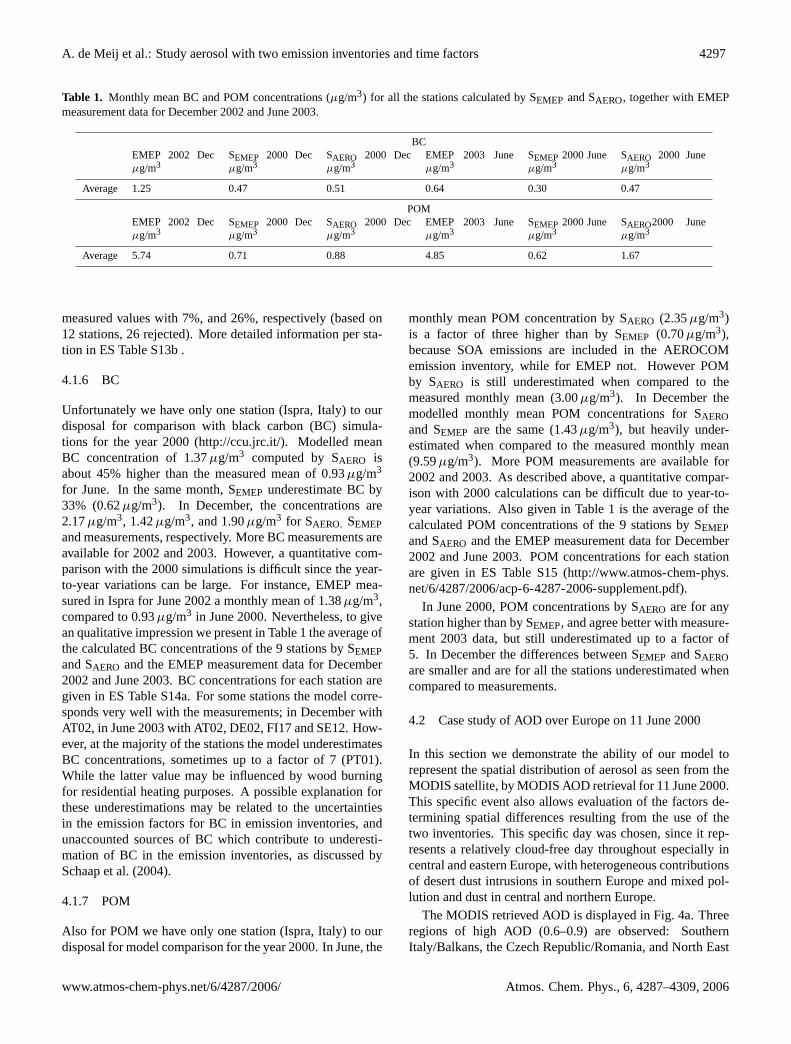
4.1.6 BC

Unfortunately we have only one station (Ispra, Italy) to ourdisposal for comparison with black carbon (BC) simula-tions for the year 2000 (http://ccu.jrc.it/). Modelled meanBC concentration of 1.37µg/m3 computed by SAERO isabout 45% higher than the measured mean of 0.93µg/m3

for June. In the same month, SEMEP underestimate BC by33% (0.62µg/m3). In December, the concentrations are2.17µg/m3, 1.42µg/m3, and 1.90µg/m3 for SAERO, SEMEPand measurements, respectively. More BC measurements areavailable for 2002 and 2003. However, a quantitative com-parison with the 2000 simulations is difficult since the year-to-year variations can be large. For instance, EMEP mea-sured in Ispra for June 2002 a monthly mean of 1.38µg/m3,compared to 0.93µg/m3 in June 2000. Nevertheless, to givean qualitative impression we present in Table 1 the average ofthe calculated BC concentrations of the 9 stations by SEMEPand SAERO and the EMEP measurement data for December2002 and June 2003. BC concentrations for each station aregiven in ES Table S14a. For some stations the model corre-sponds very well with the measurements; in December withAT02, in June 2003 with AT02, DE02, FI17 and SE12. How-ever, at the majority of the stations the model underestimatesBC concentrations, sometimes up to a factor of 7 (PT01).While the latter value may be influenced by wood burningfor residential heating purposes. A possible explanation forthese underestimations may be related to the uncertaintiesin the emission factors for BC in emission inventories, andunaccounted sources of BC which contribute to underesti-mation of BC in the emission inventories, as discussed bySchaap et al. (2004).

4.1.7 POM

Also for POM we have only one station (Ispra, Italy) to ourdisposal for model comparison for the year 2000. In June, the

monthly mean POM concentration by SAERO (2.35µg/m3)is a factor of three higher than by SEMEP (0.70µg/m3),because SOA emissions are included in the AEROCOMemission inventory, while for EMEP not. However POMby SAERO is still underestimated when compared to themeasured monthly mean (3.00µg/m3). In December themodelled monthly mean POM concentrations for SAEROand SEMEP are the same (1.43µg/m3), but heavily under-estimated when compared to the measured monthly mean(9.59µg/m3). More POM measurements are available for2002 and 2003. As described above, a quantitative compar-ison with 2000 calculations can be difficult due to year-to-year variations. Also given in Table 1 is the average of thecalculated POM concentrations of the 9 stations by SEMEPand SAERO and the EMEP measurement data for December2002 and June 2003. POM concentrations for each stationare given in ES Table S15 (http://www.atmos-chem-phys.net/6/4287/2006/acp-6-4287-2006-supplement.pdf).

In June 2000, POM concentrations by SAERO are for anystation higher than by SEMEP, and agree better with measure-ment 2003 data, but still underestimated up to a factor of5. In December the differences between SEMEP and SAEROare smaller and are for all the stations underestimated whencompared to measurements.

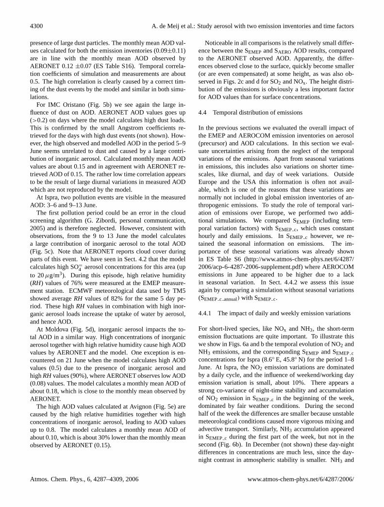
4.2 Case study of AOD over Europe on 11 June 2000

In this section we demonstrate the ability of our model torepresent the spatial distribution of aerosol as seen from theMODIS satellite, by MODIS AOD retrieval for 11 June 2000.This specific event also allows evaluation of the factors de-termining spatial differences resulting from the use of thetwo inventories. This specific day was chosen, since it rep-resents a relatively cloud-free day throughout especially incentral and eastern Europe, with heterogeneous contributionsof desert dust intrusions in southern Europe and mixed pol-lution and dust in central and northern Europe.

The MODIS retrieved AOD is displayed in Fig. 4a. Threeregions of high AOD (0.6–0.9) are observed: SouthernItaly/Balkans, the Czech Republic/Romania, and North East


http://ccu.jrc.it/




(a) (b)

(c)

Fig. 4. AOD over Europe for 11 June 10:00 GMT, 2000 by MODIS(a), AOD by SEMEP (b) and SAERO (c). White colours represent AODvalues larger than 1.5. Note that for aerosol equilibrium calculations an upper limit forRH 95% was used. No cloud masking was applied tomodel results.MODIS MOD04 L2.A2000163.1035.004.2002365174903.hdf, variable opticalDepthLand And Ocean is used.

Germany. Elsewhere the retrieved AOD was of the order of0.1–0.2. It should be noted that in other parts of Europeno aerosol was reported, due to detection of clouds by theMODIS cloud screening algorithm. Over the southern partof Italy, MODIS registers small and large Angstrom coef-ficients, indicating that both coarse (dust) and fine particlesare found in this region. Over the eastern part of EuropeMODIS registers large Angstrom coefficients, which is typ-ical for small particles, e.g. inorganic sulphate- and nitrateaerosols.

With our CTM we can compare these observations withmodel calculated AOD, but additionally, with the modelwe are able to evaluate the contributions to AOD of singleaerosol components. Figures 4b and c depicts the computedAOD distribution over Europe for 11 June 2000, 10:00 GMTfor SEMEP and SAERO, respectively. We note here that theAOD calculations are based on the relative humidity in thecloud free part of the 1◦×1◦ model grid-box (diagnosed fromthe grid-box averageRH) and that theRH should not exceed

95%. However, clouds are not “masked” in our model cal-culations. To avoid calculations of highly uncertainRH inregions with almost complete cloud cover we discard the re-gions with ECMWF cloud cover larger than 90%. The distri-bution of AOD over Europe as calculated with the two inven-tories is very similar: maximum AOD values of 1.4 (SEMEP)

and 1.6 (SAERO) are found over the western part of Germany,and bands of high AOD (0.6–0.9) are calculated over almostentire Germany, Austria, and Italy. Clean air travelling be-hind a frontal system in the western part of Europe, England,Denmark, the Netherlands, Belgium, France, and Spain is as-sociated with AOD smaller than 0.2. The high model AODgiven by the two model simulations agrees very well withMODIS over Germany and Italy, but the high AOD retrievedover the Czech Republic/Romania is underestimated by thetwo model simulations. The model calculated AOD overWestern Europe seems somewhat lower than the retrievedvalues.



Table 2. Averaged AOD values together with the corresponding correlation coefficients for June and December 2000 for all the AERONETstations used in this work. The values are based on monthly mean AOD calculated by TM5 with the EMEP emission inventory and theAEROCOM emission inventory for each station.

Monthly mean + r. Monthly mean + r. Monthly mean +sdev AOD SEMEP sdev AOD SAERO sdev AOD AERONET

June average 0.15±0.16 0.22 0.16±0.14 0.22 0.19±0.11December average 0.08±0.06 0.05 0.07±0.05 0.02 0.12±0.06

How do individual components contribute to the AOD?

A desegregation of individual components indicates thatespecially in the vicinity of Southern Italy, dust contributeswith 0.15 (or 25%) to the AOD, which is in agreement withthe MODIS observed Angstrom coefficients. In NorthernEurope dust contributes with 0.05 to the computed AODof 0.9. There the high computed AOD is caused by ele-vated concentrations of inorganic aerosols (SO=

4 , NO−

3 andNH+

4 ) and associated aerosol water (aerosol water makes upto 70% of the total aerosol mass over this area). The pres-ence of small particulate inorganic aerosols in this area isfound back in the Angstrom coefficients retrieved by MODISwhich range from 2.5 to 4. According to the ECWMF mete-orological data underlying our model, highRH (>90%) andcloud cover around 70% prevail in the western part of Ger-many and high AOD is calculated due to the uptake of largeamount of water by the inorganic aerosols. MODIS does notregister AOD at all for this area, due to the reported presenceof warm clouds. While this is consistent with the ECMWFmeteorology, MODIS does probably often discard aerosol inthe vicinity of regions with partial cloud cover and highRH.

As outlined in the previous section, the use of the AE-ROCOM emissions inventory leads to higher surface con-centrations of SO=4 and NO−

3 , because summertime emis-sions are higher. These differences are partially reflectedin the calculated AOD. As mentioned above, the AOD ge-ographical patterns of SAERO and SEMEP are similar, butover the Baltic Sea AOD difference up to 0.4 are calcu-lated, due to higher SO=4 concentrations over this area. In ESTable S11a (http://www.atmos-chem-phys.net/6/4287/2006/acp-6-4287-2006-supplement.pdf) we see that higher SO=4concentrations are calculated by SAERO than by SEMEP (upto a factor of 2) for the Finish, Swedish and Lithuanian sta-tions. Over the southern part of Italy, higher AOD valuesare calculated by SEMEP, up to 0.2 difference. For this areaSEMEP calculates higher SO=4 concentrations than SAERO, upto 9µg/m3 SO=

4 difference.

In the next section we will compare the calculated AODvalues to AERONET measurements.

4.3 Comparison of modelled AOD with AERONET

In this section we compare modelled AOD with the re-trieved AOD at a selected number of AERONET stations.While the geographic coverage of AERONET is rather lim-ited as compared to the satellite data described in the pre-vious section, we use the much higher time resolution toevaluate the temporal evolution of AOD in our model. Toensure monthly representativity we select for this compar-ison AERONET stations for which more than 50 observa-tions per month are reported; i.e. for June 9 stations andfor December only 6. An observation may represent a timespan ranging from a few minutes to 15 min. The model out-put was sampled at station location at an hourly frequency.Table 2 present the average of the observed and computed(SEMEP and SAERO) monthly mean AOD for all stations, to-gether with the temporal correlation for June and December.In ES Tables S16 and S17 (http://www.atmos-chem-phys.net/6/4287/2006/acp-6-4287-2006-supplement.pdf) the ob-served and computed (SEMEP and SAERO) monthly meanAOD and their temporal correlation for each station is givenfor June and December 2000, respectively. Correlations be-tween model and measurement are rather low and range forindividual stations between−0.04 and 0.52. On average theJune AOD of SEMEP is 5% lower than the SAERO AOD andboth simulations underestimate AERONET AOD by on av-erage 30%. Also for December both simulations underes-timate the AERONET AOD by 35%. To demonstrate thefactors contributing to temporal variability we now focus inmore detail on 5 stations in June (Figs. 5a–e) with a relativelylarge measurement records, and a widely varying geographiclocation: (i) El Arenosillo is a coastal site in Southern Spain(ii) Moldova is located in Eastern Europe, (iii) IMC Oristanois located on Sardinia in the Mediterranean Sea, (iv) Ispra islocated at the foothills of the Alps in Northern Italy and (v)Avignon is located in the South/East part of France. Apartfrom the calculated AOD, we also show the contribution ofthe dominant aerosol component to AOD.

Modelled dust had a substantial contribution to the totalAOD in El Arenosillo (Fig. 5a) around the 4, 9, 17–19, 25–27 June. Indeed on these days high AOD were observedby AERONET (up to 0.55 on 26 June) and AERONETAngstrom coefficients ranged from 0.4–1.5, indicating the







presence of large dust particles. The monthly mean AOD val-ues calculated for both the emission inventories (0.09±0.11)are in line with the monthly mean AOD observed byAERONET 0.12±0.07 (ES Table S16). Temporal correla-tion coefficients of simulation and measurements are about0.5. The high correlation is clearly caused by a correct tim-ing of the dust events by the model and similar in both simu-lations.

For IMC Oristano (Fig. 5b) we see again the large in-fluence of dust on AOD. AERONET AOD values goes up(>0.2) on days where the model calculates high dust loads.This is confirmed by the small Angstrom coefficients re-trieved for the days with high dust events (not shown). How-ever, the high observed and modelled AOD in the period 5–9June seems unrelated to dust and caused by a large contri-bution of inorganic aerosol. Calculated monthly mean AODvalues are about 0.15 and in agreement with AERONET re-trieved AOD of 0.15. The rather low time correlation appearsto be the result of large diurnal variations in measured AODwhich are not reproduced by the model.

At Ispra, two pollution events are visible in the measuredAOD: 3–6 and 9–13 June.

The first pollution period could be an error in the cloudscreening algorithm (G. Zibordi, personal communication,2005) and is therefore neglected. However, consistent withobservations, from the 9 to 13 June the model calculatesa large contribution of inorganic aerosol to the total AOD(Fig. 5c). Note that AERONET reports cloud cover duringparts of this event. We have seen in Sect. 4.2 that the modelcalculates high SO=4 aerosol concentrations for this area (upto 20µg/m3). During this episode, high relative humidity(RH) values of 76% were measured at the EMEP measure-ment station. ECMWF meteorological data used by TM5showed averageRH values of 82% for the same 5 day pe-riod. These highRH values in combination with high inor-ganic aerosol loads increase the uptake of water by aerosol,and hence AOD.

At Moldova (Fig. 5d), inorganic aerosol impacts the to-tal AOD in a similar way. High concentrations of inorganicaerosol together with high relative humidity cause high AODvalues by AERONET and the model. One exception is en-countered on 21 June when the model calculates high AODvalues (0.5) due to the presence of inorganic aerosol andhighRHvalues (90%), where AERONET observes low AOD(0.08) values. The model calculates a monthly mean AOD ofabout 0.18, which is close to the monthly mean observed byAERONET.

The high AOD values calculated at Avignon (Fig. 5e) arecaused by the high relative humidities together with highconcentrations of inorganic aerosol, leading to AOD valuesup to 0.8. The model calculates a monthly mean AOD ofabout 0.10, which is about 30% lower than the monthly meanobserved by AERONET (0.15).

Noticeable in all comparisons is the relatively small differ-ence between the SEMEP and SAERO AOD results, comparedto the AERONET observed AOD. Apparently, the differ-ences observed close to the surface, quickly become smaller(or are even compensated) at some height, as was also ob-served in Figs. 2c and d for SO2 and NOx. The height distri-bution of the emissions is obviously a less important factorfor AOD values than for surface concentrations.

4.4 Temporal distribution of emissions

In the previous sections we evaluated the overall impact ofthe EMEP and AEROCOM emission inventories on aerosol(precursor) and AOD calculations. In this section we eval-uate uncertainties arising from the neglect of the temporalvariations of the emissions. Apart from seasonal variationsin emissions, this includes also variations on shorter time-scales, like diurnal, and day of week variations. OutsideEurope and the USA this information is often not avail-able, which is one of the reasons that these variations arenormally not included in global emission inventories of an-thropogenic emissions. To study the role of temporal vari-ation of emissions over Europe, we performed two addi-tional simulations. We compared SEMEP (including tem-poral variation factors) with SEMEP c, which uses constanthourly and daily emissions. In SEMEP c however, we re-tained the seasonal information on emissions. The im-portance of these seasonal variations was already shownin ES Table S6 (http://www.atmos-chem-phys.net/6/4287/2006/acp-6-4287-2006-supplement.pdf) where AEROCOMemissions in June appeared to be higher due to a lackin seasonal variation. In Sect. 4.4.2 we assess this issueagain by comparing a simulation without seasonal variations(SEMEP c annual) with SEMEP c.

4.4.1 The impact of daily and weekly emission variations

For short-lived species, like NOx and NH3, the short-termemission fluctuations are quite important. To illustrate thiswe show in Figs. 6a and b the temporal evolution of NO2 andNH3 emissions, and the corresponding SEMEP and SEMEP cconcentrations for Ispra (8.6◦ E, 45.8◦ N) for the period 1–8June. At Ispra, the NO2 emission variations are dominatedby a daily cycle, and the influence of weekend/working dayemission variation is small, about 10%. There appears astrong co-variance of night-time stability and accumulationof NO2 emission in SEMEP c in the beginning of the week,dominated by fair weather conditions. During the secondhalf of the week the differences are smaller because unstablemeteorological conditions caused more vigorous mixing andadvective transport. Similarly, NH3 accumulation appearedin SEMEP c during the first part of the week, but not in thesecond (Fig. 6b). In December (not shown) these day-nightdifferences in concentrations are much less, since the day-night contrast in atmospheric stability is smaller. NH3 and





(a) (b)

(c) (d)

(e)

Fig. 5. Total AOD of TM5 with EMEP emission inventory (red line) and AEROCOM emission inventory (blue line) and AERONETAOD (black stars), together with the AOD of the component which has the largest contribution to the total AOD, for El Arenosillo(a),IMC Oristano(b), Ispra(c), Moldova(d) and Avignon(e). Brown presents AOD by dust for AEROCOM (a, b) or inorganic aerosol and theassociated water for (c–e). Green AOD by dust (a, b) or by inorganic aerosol and the associated aerosol water for (c–e).

NOx concentrations by SEMEP are in general lower than bySEMEP c.

We analyse in ES Table S18 the significance of this com-paring the modelled concentrations for the simulations withand without the temporal distribution, and when possible also



(a) (b)

Fig. 6. The temporal distribution of NO2 (a) and NH3 (b) emissions together with the modelled concentrations with and without temporalvariation, for Ispra, June 2000.

Table 3. Averaged concentrations and the corresponding standard deviation of all stations of the aerosol precursor gases NH3 and NOx forwhich the correlation coefficient for calculated NOx between SEMEP and SEMEP c in June is<0.8.

NH3 ppb NOx ppbSEMEP SEMEP C r SEMEP SEMEP C r EMEP data

June average 3.84±2.07 3.99±2.26 0.78 4.85±1.68 5.11±1.72 0.56 4.71±1.70December aver-age

2.60±1.85 2.54±1.70 0.85 9.37±6.40 9.36±6.22 0.94 8.53±4.09

with available observations. We analyzed the 14 EMEP mea-surement locations (44 rejected), for which the deviation be-tween the two simulations was found to be important (i.e.nearby regions of high emissions). The correlation coeffi-cient for calculated NOx between SEMEP and SEMEP c forthese 14 stations in June is<0.8, indicating the importanceof the daily and weekly distribution of the NOx emissions.The average concentrations of NH3 and NOx for all the sta-tions by SEMEP and SEMEP c for June and December is givenin Table 3.

For June the monthly averaged NH3 and NOx concentra-tions are on average and in almost all cases somewhat lowerwhen daily and weekly emission variations are taken into ac-count, up to 13% for NOx and 25% for NH3. Correlationcoefficients of hourly modelled concentrations at the selectedlocations are between 0.29–0.74 for NOx, and between 0.65–0.89 for NH3 (ES Table S18a,http://www.atmos-chem-phys.net/6/4287/2006/acp-6-4287-2006-supplement.pdf). The re-sults of the modelled NOx concentrations of both simulationsagree on average very well with both observations.

We have very few representative NH3 measurement dataavailable; e.g. for NH3 in the Netherlands (NL10) calculatedby SEMEP is lower (5.90 ppb) than by SEMEP c (6.42 ppb), butis for both cases far below the measured value of 23 ppb. At

HU02 NH3 SEMEP is 3.01 ppb and NH3 SEMEP c is 3.20 ppb,which agrees better to the measured mean concentration of3.52 ppb. It seems that the spatial variability of measuredNH3 is too large to prove that the modelled NH3 improveswhen including high time resolution.

In December, SEMEP and SEMEP c, correlate on aver-age better than in June, and the concentrations deviate lessstrongly, indicating that also in other regions, in winterboundary layer mixing plays a less important role. Clearlyincluding the hourly and daily emission-variability can notexplain all model-measurement differences.

Differences in precursor concentrations (NH3, NOx) leadto differences in the calculated nitrate aerosol, which aresmaller in all cases for SEMEP in June (up to 30%). In De-cember, when model results of SEMEP and SEMEP c can becompared to artefact-free NO−3 aerosol measurements (ESTable S19, 16 stations, including stations with temporal cor-relation coefficient smaller than 0.5) differences are rathersmall and do not lead to a clear improvement. For mostlonger-lived species the impact of daily and weekly emis-sions factors is smaller than 1–2%. The explanation for thisobservation is that for species that have a lifetime of morethan a day, advective fluxes are dominating and mask theshort-term emission variations.





Table 4. Averaged computed (SEMEP and SEMEP c) and observed NO−3 aerosol concentrations, together with the corresponding temporalcorrelation coefficient of all the stations, for December 2000.

December NO−3 aerosolMonthly meanppb SEMEP

r Monthly meanppb SEMEP C

r EMEP ppbmeasurements

December aver-age

1.40±0.93 0.45 1.41±0.92 0.44 0.93±0.62

Table 5. Averaged computed (SEMEP c and SEMEP annual) and observed SO=4 aerosol, BC and POM concentrations and the correspondingtemporal correlation coefficient of all the stations, for June 2000.

SO=4 ppb SEMEP c SO=

4 ppb SEMEP C annual EMEP ppb data

Average 0.64±0.50 0.72±0.56 0.60±0.39BC µg/m3 SEMEP c BC µg/m3 SEMEP C annual EMEP data June 2003µg/m3

Average 0.31±0.20 0.40±0.26 0.64POMµg/m3 SEMEP c POMµg/m3 SEMEP C annual OC EMEP data June 2003µg/m3

Average 0.63±0.47 0.76±0.54 4.85

4.4.2 The impact of monthly emission variations

In this section we show that the seasonal distribution ofemissions has a stronger impact on simulated SO=

4 , BCand POM concentrations than the hourly and daily varia-tions. In our discussion we focus on June, similar effectsbut opposite in sign can be found for December. In ESTable S20 (http://www.atmos-chem-phys.net/6/4287/2006/acp-6-4287-2006-supplement.pdf) we present the monthlymean concentrations for sulphate aerosol, BC and POM forJune 2000. For BC and POM we compare measurement dataof June 2003 (no measurement data available for 2000).

In June, the use of annual average emissions(SEMEP c annual) leads in general to higher emissions ofe.g. SO2 and NOx, since the intensity of residential andcommercial heating, is less during summer than in winter.As a consequence, aerosol and aerosol precursor concen-trations are generally higher in simulation SEMEP c annual.For instance, at Jarczew (PL02) the monthly mean SO2concentration increases from 1.57 ppb (SEMEP c) to 2.26 ppb(SEMEP c annual); compared to a measured monthly meanof 1.57 ppb. For NH3 again large differences up to 30% atthe stations between SEMEP c and SEMEP c annualare found.NH3 concentrations computed by SEMEP c are higher, whichdemonstrates the application of higher emission factors forNH3 emissions during the summer months (agriculturalactivities are higher during summer months than in winter);but again it is difficult to discern better model performanceon the basis of a few stations.

Differences in NOx concentrations between SEMEP c andSEMEP c annualare small (up to 8% higher by SEMEP c annual).For the majority of the stations the NOx concentrations by

SEMEP c annual agree a little better with measurement data.However, on average, the modelled NOx concentrations ofSEMEP c and SEMEP c annual are the same (5.71 ppb) and inreasonable agreement with the measured values (4.48 ppb;27% higher).

The larger SO2 emissions also increase the calculated SO=

4concentrations comparing SEMEP c annualwith SEMEP c. Forsulphate aerosol we have a substantial amount of measure-ments available allowing for robust evaluation of the im-provement resulting from using seasonally resolved emis-sions. Like in Sect. 4.1, in our analysis we excluded 30 sta-tions for which the temporal correlation coefficient of modelresults with measurement data is less than 0.5. In June, in all41 cases SO=4 by SEMEP c is lower than by SEMEP c annual,and agree better with measurement data. The mean con-centrations averaged for all stations (Table 5) are 0.64±0.50for SEMEP c, 0.72±0.56 (ppb) for SEMEP c annualand for themeasurements 0.60±0.39 (ppb).

Monthly mean BC concentrations (Table 5) bySEMEP c annual are higher than SEMEP c (up to 50%);however on average both simulations seem to substantiallyunderestimate BC in June. Note again that we have com-pared to data obtained in June 2003, since no observationsare available for 2000. We find differences up to 40% inPOM monthly mean concentrations between the SEMEP cand SEMEP c annual. As noted before the difference with mea-sured OC is very large, associated with the neglect of SOAformation. We used a constant factor of 1.4 in the conversionfrom POM to OC. While this factor is fairly uncertain, thevalue for this factor was chosen for consistency with theassumptions made in the AEROCOM database.





Table 6. Averaged computed (SEMEP c and SEMEP annual) and observed AOD values of all the stations, together with the correspondingtemporal correlation coefficient for June 2000.

Monthly mean + sdev AODSEMEP C

r. Monthly mean + sdev AODSEMEP C annual

r. Monthly mean + sdev AODAERONET

Average 0.15±0.15 0.22 0.16±0.16 0.23 0.19±0.11

What is the impact of the emission variability on calcu-lated AOD?

The substantial differences found between the monthlyconcentrations of SEMEP c and SEMEP c annual translate inrelatively small (<10%) differences in AOD calculations,consistent with the deviation of the main contributing inor-ganic sulphate concentrations. Comparison of SEMEP c andSEMEP c annualmodelled AOD with the AERONET stations(Table 6) shows that on average AOD for SEMEP c annual(0.16) is getting slightly better agreement with AERONET(0.19) than SEMEP c (0.15). AOD values for the stations canbe found in ES, Table 21.

5 Discussion

We showed that despite the over-all annual and Europeanscale agreement, large differences in the geographical dis-tributions of EMEP and AEROCOM emission inventorieswere found. In addition we showed the strong influence ofthe recommended vertical distribution of the emissions onthe distribution of aerosol precursor gases. The differenceswere translated in relatively large divergences of NOx andSO2 concentrations where especially the AEROCOM recom-mended emissions tend to overestimate measured NOx (fromEDGAR3.2 database), SO2 and to a lesser extend SO=

4 con-centrations for June 2000 when compared with EMEP mea-surement data.

Some studies (e.g. Pont and Fontan, 2001; Pryor andSteyn, 1995; Jenkin et al., 2002) have previously evaluatedthe impact of temporal distribution of emissions on O3 con-centrations. These studies demonstrated that the temporalvariation of precursor emissions NOx and VOC are resultingin a day-of-week dependence of O3 concentrations. Schaapet al. (2003) showed the role of seasonal variation of NH3emissions on the NH3 and NO3 aerosol calculations. Ourstudy confirmed latter study that the daily and weekly distri-bution of emissions is important for NH3, NOx and NO3 cal-culations. In addition we demonstrated that the additional in-formation from daily and weekly time resolution is not veryimportant for SO2, and SO=4 , BC and POM calculations;however monthly variations of the emissions can stronglyimpact the calculated concentrations. Therefore, a major im-provement of the current global inventories of aerosol andaerosol precursor would be a systematic evaluation of the

seasonal cycle of anthropogenic emissions. The strong in-fluence of the emission height on our calculations was some-what surprising. Processing of emission in models seems tobe more important than emissions themselves, indicating thateach model has “a mind of its own”, and therefore largely in-dependent of emissions input. Similar results were obtainedwhen harmonizing aerosol emissions in AeroCom Exp. B,Textor et al. (2006). Little information is available on emis-sion heights of anthropogenic emissions. The recommendedemissions height used for AEROCOM inventory was basedon expert judgement and not on data; whereas the EMEPheight recommendation is based on only very few bottom-upstudies on emission heights; and the recommendations maybe strongly biased. Surprisingly within Europe there is nocompilation available about the stack-heights of large pointsource; nor about the plume rise associated with them. Ef-fective plume rise of other sources are not known.

We showed that a further uncertainty is introduced by thedesegregation of PM2.5 emissions in the EMEP inventoryinto aerosol components; where especially BC concentra-tions are for both the months underestimated compared tothe measurement data. A bottom-up approach retaining asmuch as possible information on aerosol size and composi-tion would be desirable for future European inventories. Wefurther showed the sensitivity of model results to the assumedseasonal distribution of NH3 emissions; for which relativelylittle is available.

The AEROCOM inventory also contained pseudo-emissions for secondary organic aerosol. Indeed it wasshown that the secondary organic aerosol may several timesexceed the primary organic aerosols. At present, some globaland regional models include parameterisations of organicaerosol formation. However, as discussed by Kanakidou etal. (2005) uncertainties in the SOA formation are at least afactor of two, which results in difficult to quantify uncertain-ties in the European aerosol budget.

Despite substantial differences in calculated aerosol con-centrations at the Earth’s surface the associated AOD wasless different. In both simulations the highest AOD was re-lated to regions with high relative humidity, in the vicinity ofclouds. In these areas of highRH (>90%), large quantitiesof water on inorganic aerosol are calculated (>50µg/m3).MODIS does not report successful AOD retrieval for theseareas. Whether or not this aerosol should be classified ascloud or rather as aerosol with a large water fraction is an



(a) (b)

(c) (d)

(e)

Fig. 7. AOD calculated by the model (blue) and observed by AERONET (red) at different relative humidity ranges (40–50%, 50–60%,60–70%, 70–80%, 80–90%), for El Arenosillo(a), IMC Oristano(b), Ispra(c), Moldova(d) and Avignon(e) for June 2000. The black linepresents the standard deviation.



open question. However, we do think that these aerosols arefrequently present and are often not “seen” by satellite re-trievals.

From the model point of view the aerosol equilibriummodel used in our study (EQSAMv03d), or any other equi-librium model, is not tested for high relative humidity, ren-dering the calculations of aerosol water rather uncertain.

Whether the AOD calculation by the model strongly de-pends on theRH (influence of RH on aerosol water) ordoes the model underestimate/overestimate aerosol concen-trations, we present in Fig. 7 theRH dependency of AODcalculation.

At low RH ranges (i.e. 40–50%, 50–60%, 60–70%) we seethat the model calculated AOD is too low when compared toAERONET. This indicates that the concentrations of (inor-ganic) aerosols is too low for this areas. The larger standarddeviations for El Arenosillo at lowRH is due to the presenceof aerosol dust, leading to higher AOD peak values. The highAOD model value for Oristano atRH 40–50% is based on afew hours only and therefore not statistically robust.

At higher RH ranges (70–80%, 80–90%) larger standarddeviations are found when compared to AERONET, indicat-ing the non-linear effect ofRH on aerosol water calculations,which contribute to the overestimation of the AOD values.

We evaluated the effects of assuming the “water-solubleaerosol accumulation/aitken mode” according to the Whitbydistribution with 2 other distributions as presented in Ta-ble 4.2 in the d’Almeida climatology (r=0.0285µm andsigma=2.239) and Putaud et al. (2003) who present a hostof log-normal fits to observed size distributions at variouslocations in Europe. E.g. at the rural location Ispra Mode 2parameters r=0.024µm and sigma=1.91. Using these param-eters we calculate that the extinction coefficient would differfrom the assumed Whitby distribution by 3% (higher) and15% (lower), respectively.

6 Conclusions

Based on the analysis presented above it appears that the AE-ROCOM inventory overestimates the emissions of aerosolprecursor gases SO2 and NOx and NH3 emissions, especiallyin June. This overestimate is the combined effect of a lack inseasonal variation in the AEROCOM inventory and the dif-ferent vertical distribution of emissions (SO2 and NOx). ForNH3 is seems that the inclusion of recent abatement mea-sures in the EMEP inventory (see Sect. 2.3.3) indeed leads toa better agreement with measured concentrations.

The height distribution of the emissions is obviously a lessimportant factor for AOD values than for surface concentra-tions.

We evaluated the impact of the EMEP and AEROCOMemission inventories on aerosol concentrations and aerosoloptical depth (AOD) in Europe for June and December 2000.There are substantial differences between annual emissions

included in the two inventories, e.g. mineral dust emissionsare 40% lower and NH3 emissions are 18% higher comparingAEROCOM and EMEP emissions. The differences betweenAEROCOM and EMEP emissions are in general augmentedin June (factors of 1.00–2.48) compared to December (fac-tors 0.71–1.21).

Especially for SO2 and NOx differences occur also in thevertical distribution profile of the emissions. Despite thesedifferences, for most aerosol species and aerosol precursorgases TM5 simulates the spatial and temporal distributionover Europe relatively well. Spatial correlations, based onmonthly mean concentrations are often quite high and manyEMEP measurement stations show high temporal correlationwith SEMEP and SAERO.

However, a better agreement of surface concentrations ofaerosol precursors SO2, NOx and aerosol NH+4 are calculatedwith the EMEP emissions inventory for June, while SO=

4 forboth simulations compares well to observations. Similar dis-crepancies are found in December, with the difference thatSO=

4 is underestimated by a factor of two using both inven-tories. At the only station available in 2000 for comparison(Ispra), black carbon concentrations calculated with both in-ventories agree within±40% with the measured concentra-tions in June and December, respectively; a comparison withmeasurements from other years/locations indicated in gen-eral a large underestimate of computed BC.

The large differences in surface concentrations betweenthe simulations are not equally reflected in correspondingdifferences in computed column aerosol and AOD. In June,model AOD computations using the AEROCOM and EMEPemission inventories reveal good agreement with surfacebased AERONET sun photometer observations and AOD re-trieved from MODIS. Spatial patterns over Europe of AODdiffer due to the varying contributions of mineral dust andinorganic aerosol, as observed by satellite and confirmed bymodel simulations. An evaluation of the impact on aerosolof the temporal distribution (daily, weekly and seasonal) ofemissions reveals that the concentrations of most aerosolcomponents are not strongly influenced by introduction ofa high temporal resolution of emissions. The exception isaerosol nitrate and its precursor gases NOx, and NH3.

However, seasonal temporal variation of the emissions doplay an important role for all gas and aerosol calculations,and need to be included to accurately calculate aerosol con-centrations and its influence on climate.

Global scale emission inventories such as used for AERO-COM may provide a reasonable first estimate for computa-tion of aerosol precursor and aerosol concentrations. How-ever, global inventories will strongly benefit from informa-tion from regional scale inventories, such as EMEP, espe-cially with regard to knowledge on seasonality of emissions,and spatial and vertical distribution of these emissions. Thechallenge for future global inventories will be to include thisregional knowledge, while maintaining the global consis-tency and transparency.



Acknowledgements.We acknowledge S. Metzger who provided theEQSAM v03d aerosol module and O. Boucher for providing hisMie code.

Monthly and daily emission distributions have been prepared by theInstitute of Energy Economics and the Rational Use of Energy, Uni-versity of Stuttgart (D). The hourly variations are provided by TNOEnvironment, Energy and Process Innovation (NL).

We would like to thank EMEP for compiling the emission inventory,as used in the EURODELTA exercise (http://aqm.jrc.it/eurodelta).The AERONET principal investigators are acknowledged for theircontinuous effort in collecting AOD data. We thank Goddard Dis-tributed Active Archive Center (DAAC) for providing MODIS data.

Edited by: M. G. Lawrence

References

Bergamaschi, P., Krol, M., Dentener, F., Vermeulen, A., Meinhardt,F., Graul, R., Ramonet, M., Peters, W., and Dlugokencky, E. J.:Inverse modelling of national and European CH4emissions us-ing the atmospheric zoom model TM5, Atmos. Chem. Phys., 5,2431–2460, 2005,http://www.atmos-chem-phys.net/5/2431/2005/.

Bond, T. C., Streets, D. G., Yarber, K. F., Nelson, S. M., Woo, J.-H., and Klimont, Z.: A technology-based global inventory ofblack and organic carbon emissions from combustion, J. Geo-phys. Res., 109, D14203, doi:10.1029/2003JD003697, 2004.

Bouwman, A. F., Lee, D. S., Asman, W. A. H., Dentener, F. J., VanDer Hoek, K. W., and Olivier, J. G. J.: A global high-resolutionemission inventory for ammonia, Global Biogeochem. Cycles,11(4), 561–588, 1997.

Bouwman, A. F., Boumans, L. J. M., and Batjes, N. H.: Estimationof global NH3 volatilization loss from synthetic fertilizers andanimal manure applied to arable lands and grasslands, GlobalBiogeochem. Cycles, 16(2), 1024, doi:10.1029/2000GB001389,2002.

Charlson, R. J., Langner, J., Rodhe, H., Leovy, C. B., and Warren,S. G.: Perturbation of northern hemisphere radiative balance bybackscattering from anthropogenic sulphate aerosols, Tellus, Ser.B. 43, 152–163, 1991.

Chin, M., Chu, A., Levy, R., Remer, L., Kaufman, Y., Hol-ben., B., Eck, T., Ginoux, P., and Gao, Q.: Aerosol dis-tribution in the Northern Hemisphere during ACE-Asia: Re-sults from global model, satellite observations, and Sunphotometer measurements, J. Geophys. Res., 109, D23S90,doi:10.1029/2004JD004829, 2004.

Cofala, J., Amann, M., and Mechler, R.: Scenarios of world an-thropogenic emissions of air pollutants and methane up to 2030,Tech. rep., International Institute for Applied Systems Analysis(IIASA), Laxenburg, Austria, available from:http://www.iiasa.ac.at/rains/globalemiss/globalemiss.html, 2005.

d’Almedia, G. A.: A model for Saharan dust transport, J. Climatol.Appl. Meteorol., 25, 903–916, 1986.

Dentener, F. J. and Crutzen, P. J.: Reaction of N2O5 on troposphericaerosols: Impact on the global distributions of NOx, O3, and OH,J. Geophys. Res. 98, 7149–7163, 1993.

Dentener, F. J. and Crutzen, P. J.: A three-dimensional model of theglobal ammonia cycle, J. Atmos. Chem., 19, 331–369, 1994.

Dentener, F., Weele, M. V., Krol, M. C., Houweling, S., andVelthoven, P. V.: Trends and inter-annual variability of methaneemissions derived from 1979–1993 global CTM simulations, At-mos. Chem. Phys., 3, 73–88, 2003,http://www.atmos-chem-phys.net/3/73/2003/.

Dentener, F., Kinne, S., Bond, T., Boucher, O., Cofala, J., Generoso,S., Ginoux, P., Gong, S., Hoelzemann, J. J., Ito, A., Marelli, L.,Penner, J., Putaud, J.-P., Textor, C., Schulz, M., Van der Werf, G.R., and Wilson, J.: Emissions of primary aerosol and precursorgases in the years 2000 and 1750 prescribed data-sets for Aero-Com, Atmos. Chem. Phys. Discuss., 6, 2703–2763, 2006,http://www.atmos-chem-phys-discuss.net/6/2703/2006/.

Downing, H. D. and Williams, D.: Optical constants of water in theinfrared, J. Geophys. Res., 80, 1656–1661, 1975.

Eck, T. F., Holben, B. N., Reid, J. S., Dubovik, O., Smirnov, A.,O’Neill, N. T., Slutsker, I., and Kinne, S.: Wavelength depen-dence of the optical depth of biomass burning, urban and desertdust aerosols, J. Geophys. Res., 104, 31 333–31 350, 1999.

EMEP: Transboundary acidification, eutrophication and groundlevel ozone in Europe, Status report 1/2004, Norwegian Mete-orological Institute, ISSN 0806-4520, August 2004.

Ganzeveld, L., Lelieveld, J., and Roelofs, G.-J.: A dry depositionparameterization for sulfur oxides in a chemistry and general cir-culation model, J. Geophys. Res., 103, 5679–5694, 1998.

Gerber, H. E.: Relative-humidity parameterization of the Navyaerosol model (NAM), NRL Rep. 8956, Natl. Res. Lab., Wash-ington, D.C., 1985.

Gery, M. W., Whitten, G. Z., and Killus, J. P.: Development andtesting of the CBM-IV for urban and regional modelling, EPA-600/3-88-012. U.S. EPA, Research Triangle Park, 1989.

Gery, M. W., Whitten, G. Z., Killus, J. P., and Dodge, M. C.: Aphotochemical kinetics mechanism for urban and regional scalecomputer modelling, J. Geophys. Res., 94D, 12 925–12 956,1989.

Ginoux, P., Prospero, J. M., Torres, O., and Chin, M.: Long-term simulation of global dust distribution with the GOCARTmodel: Correlation with North Atlantic Oscillation., Env. Mod.and Soft., 19(2), 113–128, 2004.

Gong, S. L., Barrie, L. A., and Lazare, M.: Canadian AerosolModule (CAM): A size-segregated simulation of atmosphericaerosol processes for climate and air quality models 2. Globalsea-salt aerosol and its budgets, J. Geophys. Res., 107(D24),4779, doi:10.1029/2001JD002004, 2002.

Gong, S. L. and Barrie, L. A.: Simulating the impact of sea salt onglobal nss sulphate aerosols, J. Geophys. Res., 108(D16), 4516,doi:10.1029/2002JD003181, 2003.

Gong, S. L.: A parameterization of sea-salt aerosol source functionfor sub- and super-micron particles, Global Biogeochem. Cycles,17(4), 1097, doi:10.1029/2003GB002079, 2003.

Guelle, W., Balkanski, Y. J., Schultz, M., Dulac, F., and Monfray,P.: Wet deposition in a global size-dependent aerosol transportmodel, 1. Comparison with 1 year 210Pb simulation with groundmeasurements, J. Geophys. Res., 103, 11 429–11 445, 1998.

Halmer, M. M., Schmincke, H. U., and Graf, H. F.: The annual vol-canic gas input into the atmosphere, in particular into the strato-sphere: a global data set for the past 100 years, J. Volc. Geo. Res.115, 511–528, 2002.

Hertel, O., Berkowicz, R., and Christensen, J.: Test of two numer-ical schemes for use in atmospheric transport-chemistry models,


http://aqm.jrc.it/eurodelta

http://www.atmos-chem-phys.net/5/2431/2005/

http://www.iiasa.ac.at/rains/global_emiss/global_emiss.html

http://www.iiasa.ac.at/rains/global_emiss/global_emiss.html


http://www.atmos-chem-phys-discuss.net/6/2703/2006/


Atmos. Environ., 27A, 16, 2591–2611, 1993.Hess, M., Koepke, P., and Schult, I.: Optical properties of aerosols

and clouds: The software package OPAC, Bull. Am. Meteorol.Soc., 79, 831–844, 1998.

Holben, B., Eck, T., Slutsker, I., Tanre, D., Buis, J., Vermote, E.,Reagan, J., Kaufman, Y., Nakajima, T., Lavenau, F., Jankowiak,I., and Smirnov, A.: AERONET, a federated instrument networkand data-archive for aerosol characterization, Rem. Sens. Envi-ron., 66, 1–66, 1998.

Houweling, S., Dentener, F., and Lelieveld, J.: The impact of non-methane hydrocarbon compounds on tropospheric photochem-istry, J. Geophys. Res., 103, 10 637–10 696, 1998.

Jacobson, M. Z.: Strong radiative heating due to the mixing state ofblack carbon in atmospheric aerosols, Nature, 409(6821), 695–697, 2001.

Jenkin, M. E., Davies, T. J., and Stedman, J. R.: The origin andday-of-week dependence of photochemical ozone episodes in theUK, Atmos. Environ., 36, 999–1012, 2002.

Jeuken, A.: Evaluation of chemistry and climate models using mea-surements and data assimilation, PhD thesis, Eindhoven Univer-sity of Technology, 2000.

Jeuken, A., Veefkind, P., Dentener, F., Metzger, S., and Robles-Gonzalez, C.: Simulation of the aerosol optical depth over Eu-rope for August 1997 and a comparison with observations, J.Geophys. Res., 106, 28 295–28 311, 2001.

Kanakidou, M., Seinfeld, J. H., Pandis, S. N., Barnes, I., Dentener,F. J., Facchini, M. C., Van Dingenen, R., Ervens, B., Nenes, A.,Nielsen, C. J., Swietlicki, E., Putaud, J. P., Balkanski, Y., Fuzzi,S., Horth, J., Moortgat, G. K., Winterhalter, R., Myhre, C. E.L., Tsigaridis, K., Vignati, E., Stephanou, E. G., and Wilson, J.:Organic aerosol and global climate modelling: a review, Atmos.Chem. Phys., 5, 1053– 1123, 2005,http://www.atmos-chem-phys.net/5/1053/2005/.

Kasibhatla, P., Chameides, W. L., and John, J. S.: A three-dimensional global model investigation of seasonal variations inthe atmospheric burden of anthropogenic sulphate aerosols, J.Geophys. Res., 102, 3737–3759, 1997.

Kaufman, Y. J., Tanre, D., Remer, L. A., Vermote, E. F., Chu,A., and Holben, B. N.: Operational remote sensing of tropo-spheric aerosols over land form EOS-Moderate Resolution Imag-ing Spectroradiometer, J. Geophys. Res., 102, 17 051–17 065,1997.

Kettle, A. and Andreae, M.: Flux of dimethylsulfide from theoceans: A comparison of updated data sets and flux models. J.Geophys. Res., 105, 26 793–26 808, 2000.

Kiehl, J. T. and Briegleb, P. B.: The relative roles of sulphateaerosols and greenhouse gases in climate forcing, Science, 260,311–314, 1993.

Kinne, S., Schulz, M., Textor, C., Guibert, S., Bauer, S., Berntsen,T., Berglen, T., Boucher, O.,Chin, M., Dentener, F., Diehl, T.,Feichter, H., Fillmore, D., Ghan, S., Ginoux, P., Gong, S., Grini,A., Hendricks, J., Horowitz, L., Isaksen, I., Iversen, T., Koch,D., Krol, M., Lauer, A., Lamarque, J. F., Liu, X., Montanaro, V.,Myhre, G., Penner, J., Pitari, G., Reddy, S., Seland, O., Stier, P.,Takemura, T., and Tie, X.: An AeroCom initial assessment – op-tical properties in aerosol component modules of global models,Atmos. Chem. Phys., 6, 1815–1834, 2006,http://www.atmos-chem-phys.net/6/1815/2006/.

Krol, M., Houweling, S., Bregman, B., Van den Broek, M., Segers,

A., Van Velthoven, P., Peters, W., Dentener, F., and Bergamaschi,P.: The two-way nested global chemistry-transport zoom modelTM5: algorithm and applications, Atmos. Chem. Phys., 5, 417–432, 2005,http://www.atmos-chem-phys.net/5/417/2005/.

Lowenthal, D. H., Watson, J. G., and Saxena, P.: Contributions tolight extinction during project MOHAVE, Atmos. Environ., 34,2351–2359, 2000.

Metzger, S.: Gas/Aerosol partitioning: A simplified Methodfor Global Modelling, Ph.D. Thesis, University of Utrecht,http://www.library.uu.nl/vakgebieden/natuurensterrenk/11067main.html, 2000.

Metzger, S., Dentener, F., Pandis, S., and Lelieveld, J.: Gas/aerosolpartitioning: 1. A computationally efficient model, J. Geophys.Res., 107, D16, doi:1-.1029/2001JD001102, 2002.

Metzger, S., Dentener, F., Krol, M., Jeuken, A., and Lelieveld, J.:Gas/Aerosol partitioning 2. Global modeling results, J. Geophys.Res., 107(D16), 4313, doi:10.1029/2001JD001103, 2002.

Nightingale, P. D., Malin, G., Law, C. S., Watson, A. J., Liss, P. S.,Liddicoat, M. I., Boutin, J., and Upstill-Goddard, R. C.: In situevaluation of air-sea gas exchange parameterizations using novelconservative and volatile tracers, Global Biogeochem. Cycles,14(1), 373–387, 2000.

Pandis, S. N. and Seinfeld, J. H.: Sensitivity analysis of a chemicalmechanism for aqueous-phase atmospheric chemistry, J. Geo-phys. Res., 94, 1105–1126, 1989.

Peters, W., Krol, M. C., Dentener, F., Thompson, A. M., andLelieveld, J.: Chemistry-transport modeling of the satellite ob-served distribution of tropical tropospheric ozone, Atmos. Chem.Phys., 2, 103–120, 2002,http://www.atmos-chem-phys.net/2/103/2002/.

Peters, W., Krol, M. C., Bruhwiler, L., Dlugokencky, E. J., Dut-ton, G., Miller, J. B., Bergamaschi, P., Dentener, F. J., VanVelthoven, P., and Tans, P. P.: Towards regional scale in-version using a two-way nested global model: Characteriza-tion of transport using SF6, J. Geophys. Res., 109, D19314,doi:10.1029/2004JD005020, 2004.

Pham, M., Muller, J.-F, Brasseur, G. P., Granier, C., and Megie,G.: A three-dimensional study of the tropospheric sulfur cycle,J. Geophys. Res., 100(D12), 26 061–26 092, 95JD02095, 1995.

Pont, V. and Fontan, J.: Comparison between weekend and week-day ozone concentration in large cities in France, Atmos. Envi-ron., 35, 1527–1535, 2001.

Pryor, S. C. and Steyn, D. G.: Hebdomadal and diurnal cycles inozone time series from the Lower Fraser Valley, B.C., Atmos.Environ., 29(2), 1007–1019, 1995.

Putaud, J. P., Van Dingenen, R., Baltensperger, U., et al.: A Euro-pean aerosol phenomenology, Joint Research Centre, Institute forEnvironment and Sustainability, European Commission, 2003.

Remer, L. A., Kaufman, Y. J., Tanre, D., Mattoo, S., Chu, D. A.,Martins, J. V., Li, R.-R., Ichou, C., Levy, R. C., Kleidman, R. G.,Eck, T. F., Vermote, E., and Holben, B. N.: The MODIS AerosolAlgorithm, Products, and Validation, J. Atmos, Sci., Special Sec-tion, 62, 947–973, 2005.

Riemer, N., Vogel, H., Schell, B., Ackermann, I., Kessler, C., andHass, H.: Impact of the heterogeneous hydrolysis of N2O5 onchemistry and nitrate aerosol formation in the lower troposphereunder photosmog conditions, J. Geophys. Res., 108(D4), 4144,doi:10.1029/2002JD002436, 2003.





http://www.library.uu.nl/vakgebieden/natuurensterrenk/11067main.html

http://www.library.uu.nl/vakgebieden/natuurensterrenk/11067main.html



Russel, G. and Lerner J.: A new finite-differencing scheme forthe tracer transport equation, J. Appl. Meteorol., 20, 1483–1498,1981.

Schaap, M.: On the importance of aerosol nitrate in Eu-rope, Data analysis and modelling, Ph.D. thesis Univer-sity of Utrecht, http://www.library.uu.nl/digiarchief/dip/diss/2003-1209-110044/inhoud.htm, 2003.

Schaap, M., Van Loon, M., Ten Brink, H. M., Dentener, F., andBuiltjes, P. J. H.: The nitrate aerosol field over Europe: simula-tions with an atmospheric chemistry-transport model of interme-diate complexity, Atmos. Chem. Phys., 3, 5919–5976, 2003,http://www.atmos-chem-phys.net/3/5919/2003/.

Schaap, M., Denier van der Gon, H. A. C., Visschedijk, A. J. H.,Van Loon, M., ten Brink, H. M., Dentener, F. J., Putaud, J.-P.,Guillaume, B., Liousse, C., and Builtjes, P. J. H.: Anthropogenicblack carbon and fine aerosol distribution over Europe, J. Geo-phys. Res., 109, D18201, doi:10.1029/2003JD004330, 2004.

Schnaiter, M., Horvath, H., Mohler, O., Naumann, K. H., Saathoff,H., and Schock, O. W.: UV-VIS-NIR spectral optical proper-ties of soot and soot-containing aerosols, J. Aerosol. Sci., 34(10),1421–1444, 2003.

Shettle, E. P. and Fenn, R. W.: Models for the Aerosols for theLower Atmosphere and the Effects of Humidity Variations onTheir Optical Properties, AFGL-TR-79-0214, Environ. Res. Pa-pers, No. 676, 1979.

Sokolik, I. N. and Toon, O. B.: Incorporation of mineral compo-sition into models of the radiative properties of mineral aerosolfrom UV to IR wavelengths, J. Geophys. Res., 104, 9423–9444,1999.

Tanre, D., Kaufman, Y. J., Herman, M., and Mattoo, S.: Remotesensing of aerosol over oceans from EOS-MODIS, J. Geophys.Res., 102, 16 971–16 988, 1997.

Textor, C., Schulz, M., Guibert, S., Kinne, S., Bauer, S., Balkanski,Y., Berntsen, T., Berglen, T., Boucher, O., Chin, M., Dentener, F.,Diehl, T., Feichter, H., Fillmore, D., Ghan, S., Ginoux, P., Gong,S., Grini, A., Hendricks, J., Horrowitz, L., Isaksen, I., Iversen,T., Kirkevag, A., Koch, D., Kristjansson, J. E., Krol, M., Lauer,A., Lamarque, J. F., Liu, X., Montanaro, V., Myhre, G., Penner,J., Pitari, G., Reddy, S., Seland, O., Stier, P., Takemura, T., andTie, X.: Analysis and quantification of the diversities of aerosollife cycles within AeroCom, Atmos. Chem. Phys., 6, 1777–1813,2006,http://www.atmos-chem-phys.net/6/1777/2006/.

Tiedtke, M.: A comprehensive mass flux scheme for cumulusparameterisation in large scale models, Mon. Wea. Rev., 177,1779–1800, 1989.

Van der Werf, G. R., Randerson, J. T., Collatz, G. J., and Giglio, L.:Carbon emissions from fires in tropical and subtropical ecosys-tems, Global Change Biology, 9(4), 547–562, 2003.

Vignati, E., Krol, M., and Dentener, F.: Global and regional aerosolmodelling: a picture over Europe, in: Advances in Air Pollu-tion Modeling for Environmental Security, edited by: Farago, I.,Georgiev, K., and Havasi, A., 373–381, 2005.


http://www.library.uu.nl/digiarchief/dip/diss/2003-1209-110044/inhoud.htm

http://www.library.uu.nl/digiarchief/dip/diss/2003-1209-110044/inhoud.htm



and physics the sensitivity of aerosol in europe to two

Documents