1

Markov Decision Processes

Andrew SchaeferEWO Seminar

October 26, 2006

2

What are Markov Decision Processes (MDPs)?

MDPs are a method for formulating and solving stochastic and dynamic decisionsMDPs are very flexible, which is an advantage from a modeling perspective but a drawback from a solution viewpoint (can’t take advantage of special structure)MDPs are pervasive; every Fortune 500 company uses them in some form or anotherParticular success in inventory management and reliability

3

Potential for MDPs in EWOThe flexibility of MDPs may allow them to be useful for certain problems

It is unlikely that they can work as stand-alone techniques

Long history of successful applications

4

OutlineBasic Components of MDPs

Solution Techniques

Extensions

Big Picture – Potential Roles for MDPs

5

Outline – Basic ComponentsInventory Example

MDP Vocabulary5 Basic Components1. decision epochs2. states3. actions4. rewards5. transition probabilitiesvalue functiondecision rulepolicy

6

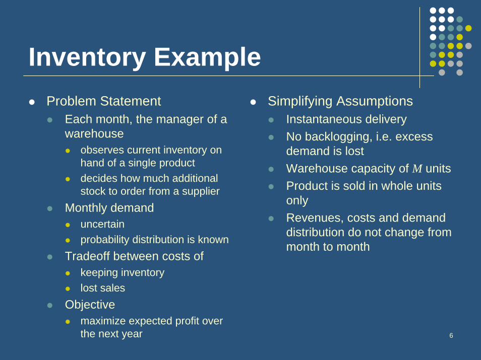
Inventory ExampleProblem Statement

Each month, the manager of a warehouse

observes current inventory on hand of a single productdecides how much additional stock to order from a supplier

Monthly demand uncertainprobability distribution is known

Tradeoff between costs ofkeeping inventory lost sales

Objective maximize expected profit over the next year

Simplifying AssumptionsInstantaneous deliveryNo backlogging, i.e. excess demand is lostWarehouse capacity of M unitsProduct is sold in whole units onlyRevenues, costs and demand distribution do not change from month to month

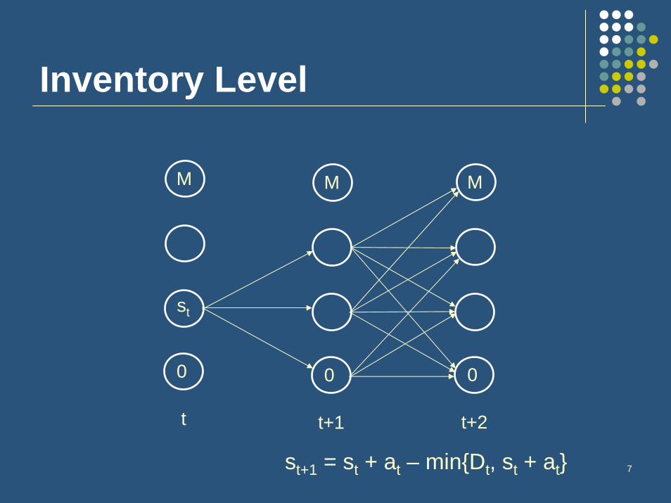
7st+1 = st + at – min{Dt, st + at}

t

M

st

0

Inventory Level

t+1

M

0

t+2

M

0

8

Outline – Basic ComponentsInventory Example

MDP Vocabulary5 Basic Components1. decision epochs2. states3. actions4. rewards5. transition probabilitiesvalue functiondecision rulepolicy

9

1. Decision Epochs: tPoints in time at which decisions are made

analogous to period start times in a “Markov Process”

Inventory examplefirst day of month 1, first day of month 2, …, first day of month 12

In general: 1, 2, …, NN: length of the time horizon (could be infinite)

Also calledperiodsstages

10

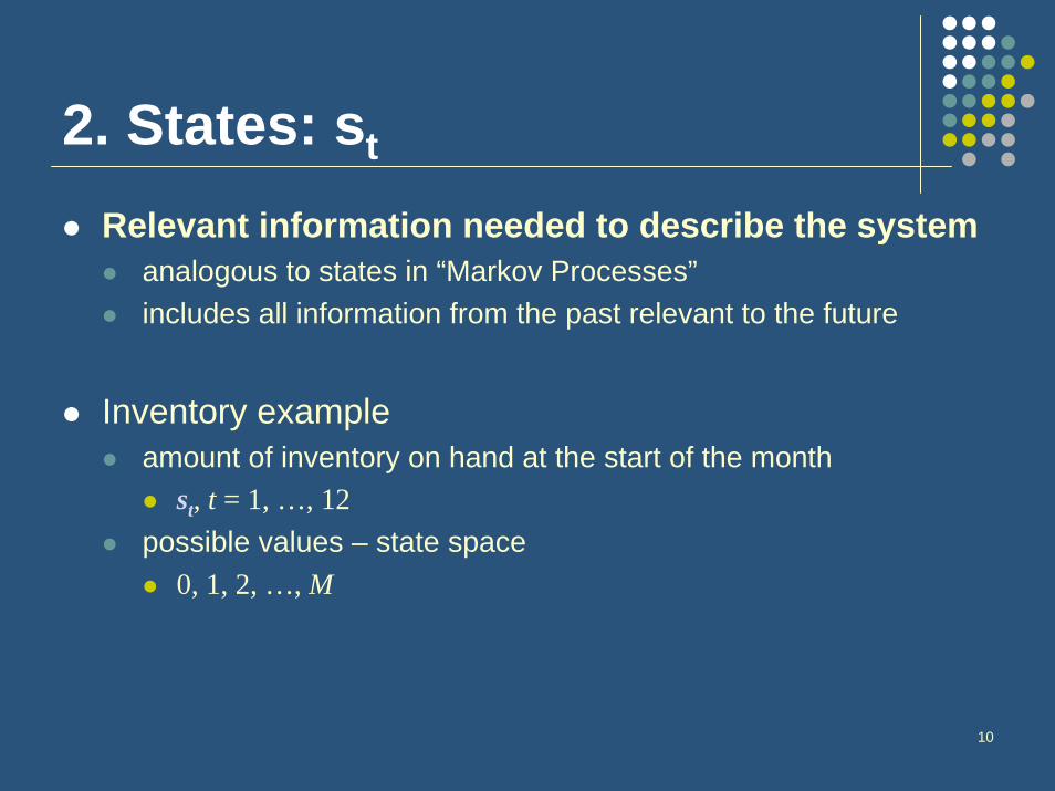
2. States: st

Relevant information needed to describe the systemanalogous to states in “Markov Processes”includes all information from the past relevant to the future

Inventory exampleamount of inventory on hand at the start of the month

st, t = 1, …, 12possible values – state space

0, 1, 2, …, M

11

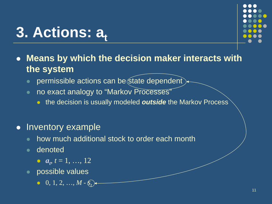
3. Actions: at

Means by which the decision maker interacts with the system

permissible actions can be state dependentno exact analogy to “Markov Processes”

the decision is usually modeled outside the Markov Process

Inventory examplehow much additional stock to order each monthdenoted

at, t = 1, …, 12possible values

0, 1, 2, …, M - st

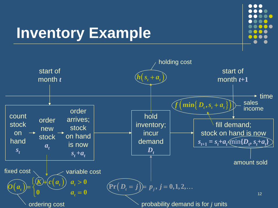
12

Inventory Example

start of month t

start of month t+1

count stock

on hand

st

order new stock

at

order arrives; stock

on hand is now st +at

fill demand; stock on hand is now

st+1 = st+at-min{Dt, st+at}

hold inventory;

incur demand

Dt

( ) ( ) 00 0

t tt

t

K c a aO a

a⎧ + >

= ⎨=⎩

time

( )t th s a+

( )Pr , 0,1,2,t jD j p j= = = …

{ }( )min ,t t tf D s a+

variable costfixed cost

ordering cost probability demand is for j units

holding cost

sales income

amount sold

13

4. Rewards: rt(st,at)Expected immediate net income associated with taking a particular action, in a particular state, in a particular epoch

analogous to state utilities in “Markov Processes”

Inventory exampleexpected income – order cost – holding cost

in the last epoch, we assume that whatever is left over has somesalvage value, g(.)

( ) ( ) ( ), E[income in month ] , 1,2, ,12t t t t t tr s a t O a h s a t= − − + = …{ } { }

( ) ( )0 1

E[income in ] E[income in | ]Pr E[income in | ]Prt t

t t

t t t t t t t t t t t ts a

j t t jj j s a

t t D s a D s a t D s a D s a

f j p f s a p+ ∞

= = + +

= ≤ + ≤ + + > + > +

= + +∑ ∑

( ) ( )13 13 13,r s g s⋅ = ( ) ( )111 , +++ =⋅ NNN sgsrin general

14

5. Transition Probabilities:pt(st,at)Distribution that governs how the state of the process changes as actions are taken over time

depends on current state and action only, and possibly timethat is, the future is independent of the past given the present(The Markov Property)

Inventory examplewe already established that st+1 = st+at-min{Dt, st+at}

can’t end up with more than you started with

end up with some leftovers if demand is less than inventoryend up with nothing if demand exceeds inventory

0ii s a

p j∞

= +

⎪⎪ =⎨⎪⎪

∑{ }1Pr | ,t t ts j s s a a+ = = = =

depends on demand0 j s a⎪ > +⎩

s a jp j s a+ − ≤ +⎧⎪

15

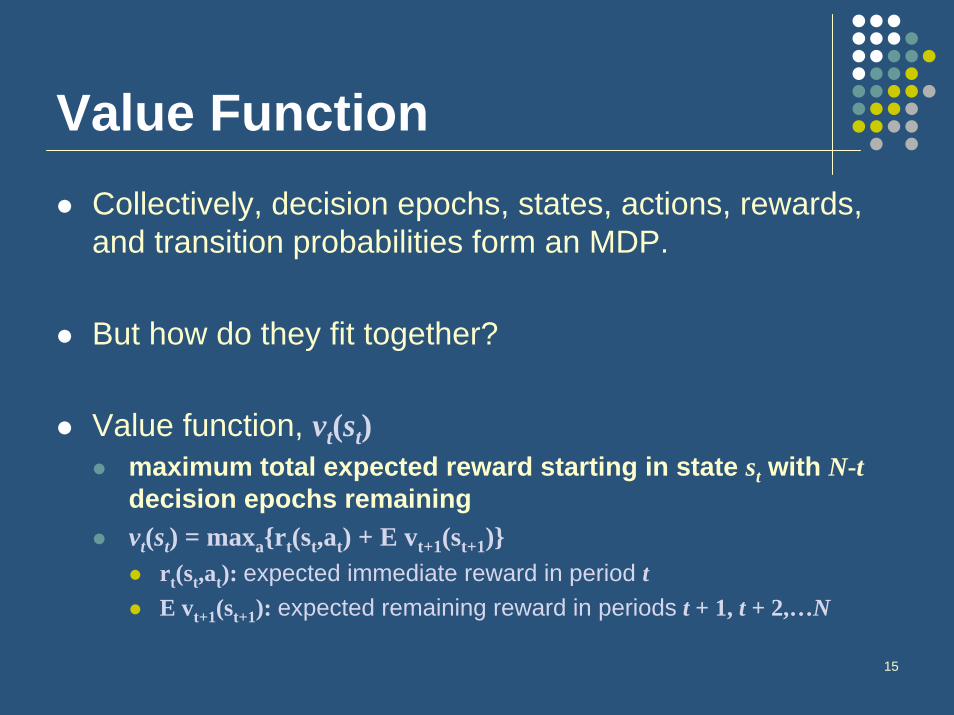
Value FunctionCollectively, decision epochs, states, actions, rewards, and transition probabilities form an MDP.

But how do they fit together?

Value function, vt(st)maximum total expected reward starting in state st with N-tdecision epochs remainingvt(st) = maxa{rt(st,at) + E vt+1(st+1)}

rt(st,at): expected immediate reward in period tE vt+1(st+1): expected remaining reward in periods t + 1, t + 2,…N

16

Value FunctionInventory example

( ) ( ) ( )

( ){ }

( ) ( ) { }

( ){ }

( ) ( ) { }

12 12

11 11

13 13 13 13 13

12 12 12 12 12 13 13 12 120,1, , 0

11 11 11 11 11 12 12 11 110,1, , 0

,

max , Pr | ,

max , Pr | ,

M

a M s j

M

a M s j

v s r s g s

v s r s a v j s j s a

v s r s a v j s j s a

∈ − =

∈ − =

= ⋅ =

⎧ ⎫= + =⎨ ⎬

⎩ ⎭⎧ ⎫

= + =⎨ ⎬⎩ ⎭

∑

∑

…

…

expected remaining reward in periods (2,…,N)

expected immediate reward period 1

( ){ }

( ) ( ) { }1 1

1 1 1 1 1 2 2 1 10,1, , 0max , Pr | ,

M

a M s jv s r s a v j s j s a

∈ − =

⎧ ⎫= + =⎨ ⎬

⎩ ⎭∑…

( ){ }

( ) ( ) { }2 2

2 2 2 2 2 3 3 2 20,1, , 0max , Pr | ,

a M s jv s r s a v j s j s a

∈ − =

= + =…

M⎧ ⎫⎨ ⎬⎩ ⎭

∑maximum total expected

reward starting in

state s1 with 12 decision

epochs remaining

17

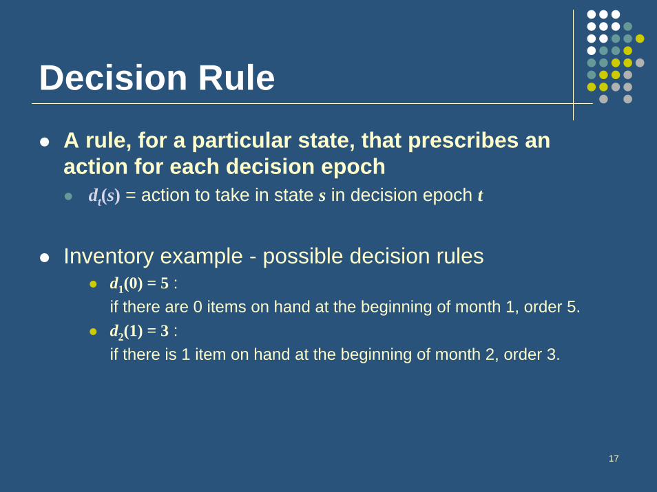
Decision RuleA rule, for a particular state, that prescribes an action for each decision epoch

dt(s) = action to take in state s in decision epoch t

Inventory example - possible decision rulesd1(0) = 5 : if there are 0 items on hand at the beginning of month 1, order 5.d2(1) = 3 :if there is 1 item on hand at the beginning of month 2, order 3.

18

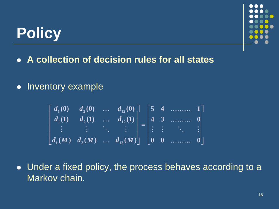
PolicyA collection of decision rules for all states

Inventory example

Under a fixed policy, the process behaves according to a Markov chain.

1 2 12

1 2 12

1 2 12

(0) (0) (0) 5 4 1(1) (1) (1) 4 3 0

( ) ( ) ( ) 0 0 0

d d dd d d

d M d M d M

⎡ ⎤ ⎡ ⎤⎢ ⎥ ⎢ ⎥⎢ ⎥ ⎢ ⎥=⎢ ⎥ ⎢ ⎥⎢ ⎥ ⎢ ⎥

⎣ ⎦⎣ ⎦

… ………… ………

… ………

19

Outline – Solution TechniquesFinite-horizon MDPs

Backwards induction solution technique

Infinite-horizon MDPsOptimality criteriaSolution techniques

value iterationpolicy iterationlinear programming

20

Various factors to consider in choosing the right technique

Will rewards be discounted?What is the objective?

Maximize expected total reward, orMaximize expected average reward

Is the problem formulated as a finite or infinite horizon problem?

If finite horizon, solution technique does not depend on discounting or objectiveFor infinite horizon, technique does depend on discounting and objective

21

Outline – Solution TechniquesFinite-horizon MDPs

Backwards induction solution technique

Infinite-horizon MDPsOptimality criteriaSolution techniques

value iterationpolicy iterationlinear programming

22

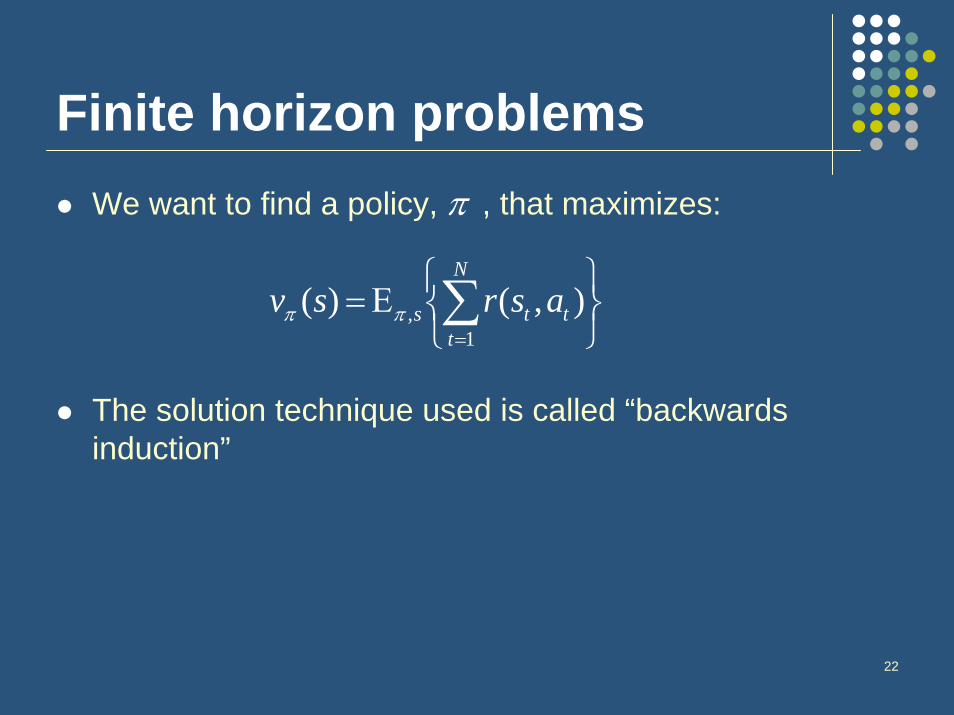
Finite horizon problemsWe want to find a policy, , that maximizes:

The solution technique used is called “backwards induction”

⎭⎬⎫

⎩⎨⎧

Ε= ∑=

N

ttts asrsv

1, ),()( ππ

π

23

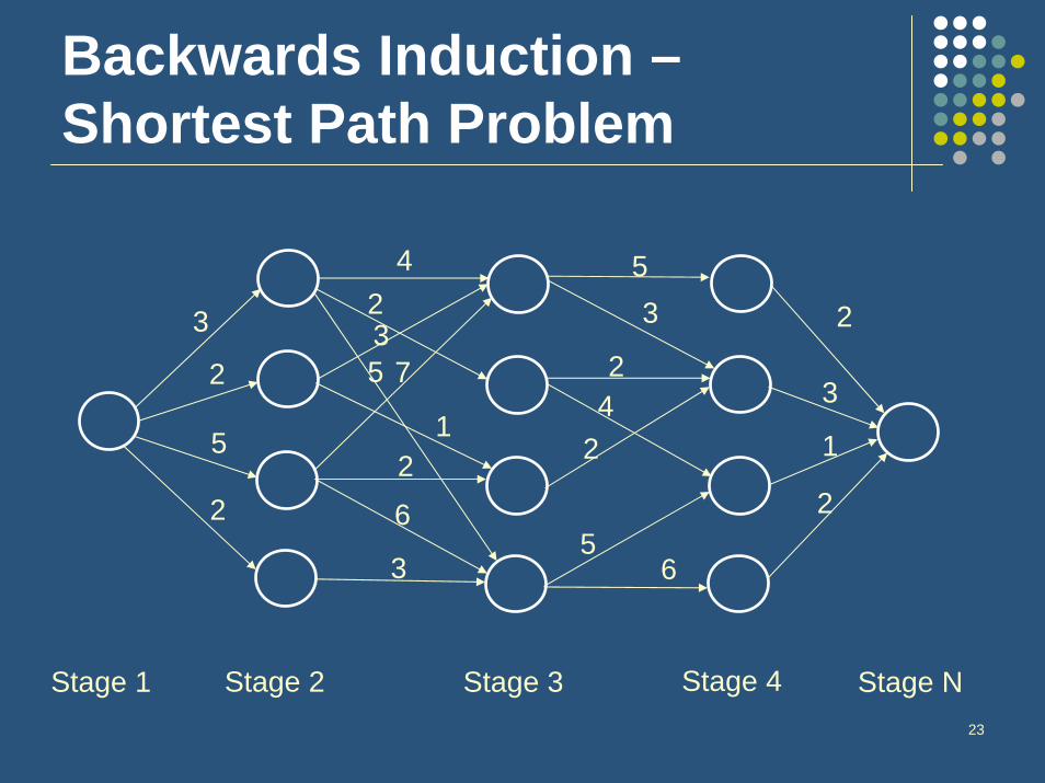
Stage 2

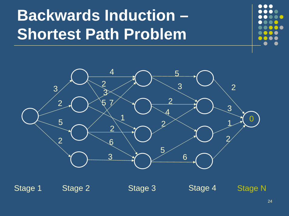
Backwards Induction –Shortest Path Problem

Stage 3 Stage 4Stage 1 Stage N

3

2

5

2

42

735

21

6

3

2

3

1

2

42

2

53

56

24

Stage 2

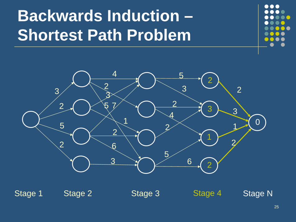
Backwards Induction –Shortest Path Problem

Stage 3 Stage 4Stage 1 Stage N

3

2

5

2

42

735

21

6

3

2

3

1

2

42

2

53

56

0

25

Stage 2

Backwards Induction –Shortest Path Problem

Stage 3 Stage 4Stage 1 Stage N

3

2

5

2

42

735

21

6

3

2

3

1

2

42

2

53

56

0

2

3

1

2

26

Stage 2

Backwards Induction –Shortest Path Problem

Stage 3 Stage N-1Stage 1 Stage N

3

2

5

2

42

735

21

6

3

2

3

1

2

42

2

53

56

0

2

3

1

2

6

5

5

6

27

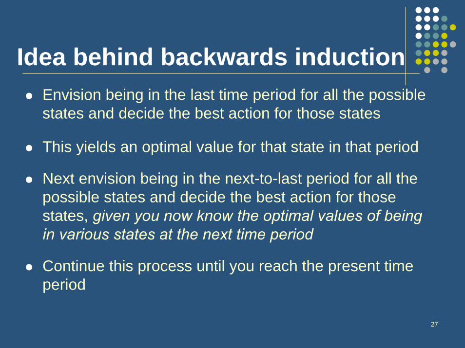
Idea behind backwards inductionEnvision being in the last time period for all the possible states and decide the best action for those states

This yields an optimal value for that state in that period

Next envision being in the next-to-last period for all the possible states and decide the best action for those states, given you now know the optimal values of being in various states at the next time period

Continue this process until you reach the present time period

28

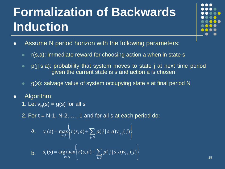
Formalization of Backwards Induction

Assume N period horizon with the following parameters:

r(s,a): immediate reward for choosing action a when in state s

p(j | s,a): probability that system moves to state j at next time period given the current state is s and action a is chosen

g(s): salvage value of system occupying state s at final period N

Algorithm:1. Let vN(s) = g(s) for all s

2. For t = N-1, N-2, …, 1 and for all s at each period do:

a.

b.

⎭⎬⎫

⎩⎨⎧

+= ∑∈

+∈ SjtAat jvasjpasrsv )(),|(),(max)( 1

⎭⎬⎫

⎩⎨⎧

+= ∑∈

+∈ Sj

tAa

t jvasjpasrsa )(),|(),(maxarg)( 1

29

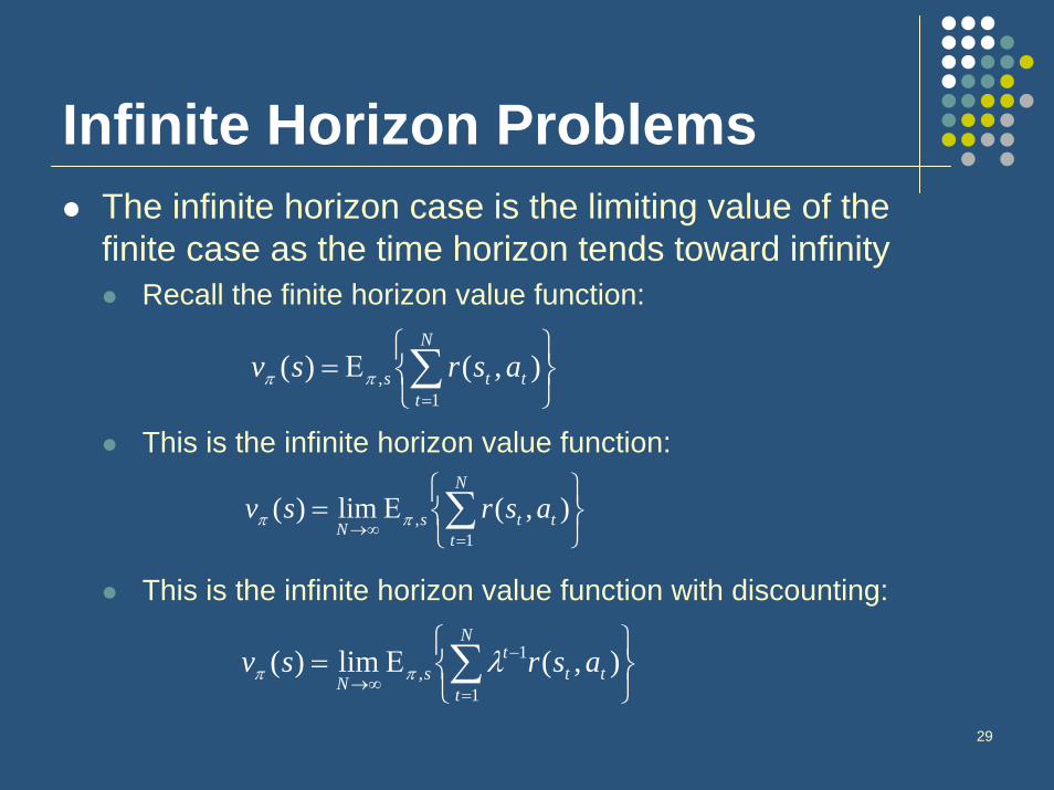
Infinite Horizon ProblemsThe infinite horizon case is the limiting value of the finite case as the time horizon tends toward infinity

Recall the finite horizon value function:

This is the infinite horizon value function:

This is the infinite horizon value function with discounting:

⎭⎬⎫

⎩⎨⎧

Ε= ∑=

N

ttts asrsv

1, ),()( ππ

⎭⎬⎫

⎩⎨⎧

Ε= ∑=

∞→

N

tttsN

asrsv1

, ),(lim)( ππ

⎭⎬⎫

⎩⎨⎧

Ε= ∑=

−

∞→

N

ttt

tsN

asrsv1

1, ),(lim)( λππ

30

Important Factors for Infinite Horizon Models

Discount factorIf we have a discount factor < 1, then total expected value converges to a finite solutionIf there is no discounting, then total expected value may explode

However, if the system has an absorbing state with 0 reward, then even these may yield finite optimal values

Objective criteriaTotal expected valueAverage expected value over the long run

More detailed analyses is required

When is a stationary optimal policy guaranteed to exist?If the state space and action space are finite

31

Previous applications of MDPsAt the heart of every inventory management paper is an MDP

Reliability and replacement problems

Some routing and logistics problems (e.g. Warren Powell’s work in trucking)

50 years of successful applications (particularly inventory theory, which is widely applied)

32

Limitations of MDPs“Curse of dimensionality”

As the problem size increases, i.e. the state and/or action space become larger, it becomes computationally very difficult to solve the MDPsThere are some methods that are more memory-efficient than Policy Iteration and Value Iteration algorithmsThere are also some solution techniques that find near-optimal solutions in a short time

Enormous data requirementsFor each action and state pair, we need a transition probabilitymatrix and a reward function

33

Limitations of MDPsStationarity assumption

In fact, transition probabilities may not stay the same over timeTwo methods to model non-stationary transition probabilities and rewards1. Use a finite-horizon model2. Enlarge the state space by including time

34

Why do MDPs not Scale Well?Analogy in the deterministic world: DP vs. IPAny integer program can be formulated as a dynamic programHowever, DPs struggle with IPs that take branch-and-bound less than a secondWhy?

IP uses polyhedral theory to get strong boundsDP techniques grow with the size of the problem

Will this occur in the stochastic setting?

35

MDP: Approximate Solution Techniques

Finding the optimal policy is polynomial time in the state space size

Linear programming formulationSometimes too many states for this to be practical

Examples of approximate solution techniquesState aggregation and action eliminationMany AI techniques (reinforcement learning)Approximate linear programming (de Farias and van Roy)In the last 10 years this has become a very active area

36

Extensions of MDPsThus far, we’ve discussed discrete-time MDP, i.e. the decisions are made at certain time periods

Continuous time MDP models generalize MDPs byallowing the decision maker to choose actions whenever the system changesmodeling the system evolution in continuous timeallowing the time spent in a particular state to follow an arbitrary probability distribution

No one has considered a continuous time stochastic program

37

Extensions of MDPsMost models are completely observable MDPs, i.e. the state of the system is known with certainty at all time periods

Partially observable MDP models generalize MDPs by relaxing the assumption that the state of the system is completely observable

38

Partially Observable MDPs(POMDPs)

System state is not fully observable.Decision maker receives a signal o which is related to the system state by q(o|s)

Observation process, depends on the (unknown) state, generated from a probability distribution function

Hidden variables form a standard MDP

ApplicationsMedical diagnosis and treatmentEquipment repair

39

POMDPs- Formal DefinitionPOMDPs consist of

State space SAction space AObservation space OTransition matrix PRewards RObservation process distribution Q(o | s)Value function V = V(y; π)

Where π: O A is a policy

40

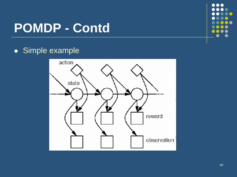
POMDP - ContdSimple example

41

POMDP controlled by parameterized stochastic policy

Dynamics of POMDP controlled by parameterized stochastic policies:

42

Constrained Markov Decision Process

MDPs with probabilistic constraintsTypically linear in terms of the limiting probability variables

ApplicationsService level constraints in call centers

P(No delay) >= 0.5E[Number in queue] <= 10

Value iteration and Policy iteration algorithms do not extend. Linear Programming does.

43

CMDP: LP techniqueCan model constraint as a function of the variables

Results in the optimal randomized policyOptimal choice of action in some states can be randomizedNot practicalDifficult to obtain the actual randomization probabilities

Why randomized?Vertices of LP polytope without constraints correspond to non-randomized policiesConstraints create new vertices corresponding to randomized policies

44

Competitive MDPsTwo (or more) players compete

The actions of one player affects the state of the other

May be interesting for modeling various oligopolisticrelationships among competitors

Still a nascent area

45

Why would I prefer an MDP to a Stochastic Program?

MDPs are much more flexible – existing multistage SP models assume linear relations across stages If there is a recursive nature to the problem, MDPs are likely superiorWhen the number of states/actions is small relative to the time horizon (e.g. inventory management) MDPs are likely to be superiorThe MDP may be easier to analyze analytically; e.g. the optimality of (s,S) policies in inventory theory

46

Why would I prefer a Stochastic Program to an MDP?

When the action and/or state space has a (good) polyhedral representationWhen the set of decisions and/or states is enormous, or infiniteWhen the number of stages is not critical relative to the detail required in each stage

47

ConclusionsMDPs are a flexible technique for stochastic and dynamic optimization problemsMDPs have a much longer history of success than stochastic programmingCurse of dimensionality may render them impractical (e.g. for a VRP, action space is set of TSP tours)Approximate solution techniques appear promisingAllow models that are unexplored in SP

Partial observabilityContinuous timeCompetition