anintroductiontoprooftheory - ucsd mathematics | …sbuss/researchweb/handbooki/chapteri.pdf ·...
TRANSCRIPT

CHAPTER I
An Introduction to Proof Theory
Samuel R. BussDepartments of Mathematics and Computer Science, University of California, San Diego
La Jolla, California 92093-0112, USA
Contents1. Proof theory of propositional logic . . . . . . . . . . . . . . . . . . . . . . . . . 3
1.1. Frege proof systems . . . . . . . . . . . . . . . . . . . . . . . . . . . . . . 51.2. The propositional sequent calculus . . . . . . . . . . . . . . . . . . . . . . 101.3. Propositional resolution refutations . . . . . . . . . . . . . . . . . . . . . . 18
2. Proof theory of first-order logic . . . . . . . . . . . . . . . . . . . . . . . . . . . 262.1. Syntax and semantics . . . . . . . . . . . . . . . . . . . . . . . . . . . . . 262.2. Hilbert-style proof systems . . . . . . . . . . . . . . . . . . . . . . . . . . 292.3. The first-order sequent calculus . . . . . . . . . . . . . . . . . . . . . . . . 312.4. Cut elimination . . . . . . . . . . . . . . . . . . . . . . . . . . . . . . . . 362.5. Herbrand’s theorem, interpolation and definability theorems . . . . . . . . 482.6. First-order logic and resolution refutations . . . . . . . . . . . . . . . . . . 59
3. Proof theory for other logics . . . . . . . . . . . . . . . . . . . . . . . . . . . . . 643.1. Intuitionistic logic . . . . . . . . . . . . . . . . . . . . . . . . . . . . . . . 643.2. Linear logic . . . . . . . . . . . . . . . . . . . . . . . . . . . . . . . . . . 70
References . . . . . . . . . . . . . . . . . . . . . . . . . . . . . . . . . . . . . . . . 74
HANDBOOK OF PROOF THEORYEdited by S. R. Bussc© 1998 Elsevier Science B.V. All rights reserved

2 S. Buss
Proof Theory is the area of mathematics which studies the concepts of mathemat-ical proof and mathematical provability. Since the notion of “proof” plays a centralrole in mathematics as the means by which the truth or falsity of mathematicalpropositions is established; Proof Theory is, in principle at least, the study ofthe foundations of all of mathematics. Of course, the use of Proof Theory as afoundation for mathematics is of necessity somewhat circular, since Proof Theory isitself a subfield of mathematics.
There are two distinct viewpoints of what a mathematical proof is. The first viewis that proofs are social conventions by which mathematicians convince one anotherof the truth of theorems. That is to say, a proof is expressed in natural languageplus possibly symbols and figures, and is sufficient to convince an expert of thecorrectness of a theorem. Examples of social proofs include the kinds of proofs thatare presented in conversations or published in articles. Of course, it is impossible toprecisely define what constitutes a valid proof in this social sense; and, the standardsfor valid proofs may vary with the audience and over time. The second view of proofsis more narrow in scope: in this view, a proof consists of a string of symbols whichsatisfy some precisely stated set of rules and which prove a theorem, which itself mustalso be expressed as a string of symbols. According to this view, mathematics canbe regarded as a ‘game’ played with strings of symbols according to some preciselydefined rules. Proofs of the latter kind are called “formal” proofs to distinguish themfrom “social” proofs.
In practice, social proofs and formal proofs are very closely related. Firstly,a formal proof can serve as a social proof (although it may be very tedious andunintuitive) provided it is formalized in a proof system whose validity is trusted.Secondly, the standards for social proofs are sufficiently high that, in order for aproof to be socially accepted, it should be possible (in principle!) to generate a formalproof corresponding to the social proof. Indeed, this offers an explanation for the factthat there are generally accepted standards for social proofs; namely, the implicitrequirement that proofs can be expressed, in principle, in a formal proof systemenforces and determines the generally accepted standards for social proofs.
Proof Theory is concerned almost exclusively with the study of formal proofs:this is justified, in part, by the close connection between social and formal proofs,and it is necessitated by the fact that only formal proofs are subject to mathematicalanalysis. The principal tasks of Proof Theory can be summarized as follows. First, toformulate systems of logic and sets of axioms which are appropriate for formalizingmathematical proofs and to characterize what results of mathematics follow fromcertain axioms; or, in other words, to investigate the proof-theoretic strength ofparticular formal systems. Second, to study the structure of formal proofs; forinstance, to find normal forms for proofs and to establish syntactic facts aboutproofs. This is the study of proofs as objects of independent interest. Third, to studywhat kind of additional information can be extracted from proofs beyond the truthof the theorem being proved. In certain cases, proofs may contain computational orconstructive information. Fourth, to study how best to construct formal proofs; e.g.,what kinds of proofs can be efficiently generated by computers?

Introduction to Proof Theory 3
The study of Proof Theory is traditionally motivated by the problem of formaliz-ing mathematical proofs; the original formulation of first-order logic by Frege [1879]was the first successful step in this direction. Increasingly, there have been attemptsto extend Mathematical Logic to be applicable to other domains; for example,intuitionistic logic deals with the formalization of constructive proofs, and logicprogramming is a widely used tool for artificial intelligence. In these and otherdomains, Proof Theory is of central importance because of the possibility of computergeneration and manipulation of formal proofs.
This handbook covers the central areas of Proof Theory, especially the math-ematical aspects of Proof Theory, but largely omits the philosophical aspects ofproof theory. This first chapter is intended to be an overview and introduction tomathematical proof theory. It concentrates on the proof theory of classical logic,especially propositional logic and first-order logic. This is for two reasons: firstly,classical first-order logic is by far the most widely used framework for mathematicalreasoning, and secondly, many results and techniques of classical first-order logicfrequently carryover with relatively minor modifications to other logics.
This introductory chapter will deal primarily with the sequent calculus, andresolution, and to lesser extent, the Hilbert-style proof systems and the naturaldeduction proof system. We first examine proof systems for propositional logic,then proof systems for first-order logic. Next we consider some applications of cutelimination, which is arguably the central theorem of proof theory. Finally, we reviewthe proof theory of some non-classical logics, including intuitionistic logic and linearlogic.
1. Proof theory of propositional logic
Classical propositional logic, also called sentential logic, deals with sentences andpropositions as abstract units which take on distinct True/False values. The basicsyntactic units of propositional logic are variables which represent atomic propo-sitions which may have value either True or False. Propositional variables arecombined with Boolean functions (also called connectives): a k -ary Boolean functionis a mapping from {T, F}k to {T, F} where we use T and F to represent True andFalse. The most frequently used examples of Boolean functions are the connectives >and ⊥ which are the 0-ary functions with values T and F , respectively; the binaryconnectives ∧ , ∨ , ⊃ , ↔ and ⊕ for “and”, “or”, “if-then”, “if-and-only-if” and“parity”; and the unary connective ¬ for negation. Note that ∨ is the inclusive-orand ⊕ is the exclusive-or.
We shall henceforth let the set of propositional variables be V = {p1, p2, p3, . . .} ;however, our theorems below hold also for uncountable sets of propositional variables.The set of formulas is inductively defined by stating that every propositional variableis a formula, and that if A and B are formulas, then (¬A), (A∧B), (A∨B), (A ⊃ B),etc., are formulas. A truth assignment consists of an assignment of True/False valuesto the propositional variables, i.e., a truth assignment is a mapping τ : V → {T, F} .

4 S. Buss
A truth assignment can be extended to have domain the set of all formulas in theobvious way, according to Table 1; we write τ(A) for the truth value of the formula Ainduced by the truth assignment τ .
Table 1Values of a truth assignment τ
A B (¬A) (A ∧B) (A ∨B) (A ⊃ B) (A ↔ B) (A⊕B)T T F T T T T FT F F F T F F TF T T F T T F TF F T F F T T F
A formula A involving only variables among p1, . . . , pk defines a k -ary Booleanfunction fA , by letting fA(x1, ..., xk) equal the truth value τ(A) where τ(pi) = xi
for all i . A language is a set of connectives which may be used in the formation ofL-formulas. A language L is complete if and only if every Boolean function can bedefined by an L-formula. Propositional logic can be formulated with any complete(usually finite) language L — for the time being, we shall use the language ¬ , ∧ , ∨and ⊃ .
A propositional formula A is said to be a tautology or to be (classically) valid ifA is assigned the value T by every truth assignment. We write ² A to denote thatA is a tautology. The formula A is satisfiable if there is some truth assignment thatgives it value T . If Γ is a set of propositional formulas, then Γ is satisfiable if thereis some truth assignment that simultaneously satisfies all members of Γ. We sayΓ tautologically implies A , or Γ ² A , if every truth assignment which satisfies Γ alsosatisfies A .
One of the central problems of propositional logic is to find useful methods forrecognizing tautologies; since A is a tautology if and only if ¬A is not satisfiable, thisis essentially the same as the problem of finding methods for recognizing satisfiableformulas. Of course, the set of tautologies is decidable, since to verify that a formula Awith n distinct propositional variables is a tautology, one need merely check thatthe 2n distinct truth assignments to these variables all give A the value T . Thisbrute-force ‘method of truth-tables’ is not entirely satisfactory; firstly, because it caninvolve an exorbitant amount of computation, and secondly, because it provides nointuition as to why the formula is, or is not, a tautology.
For these reasons, it is often advantageous to prove that A is a tautology insteadof using the method of truth-tables. The next three sections discuss three commonlyused propositional proof systems. The so-called Frege proof systems are perhaps themost widely used and are based on modus ponens. The sequent calculus systemsprovide an elegant proof system which combines both the possibility of elegant proofsand the advantage of an extremely useful normal form for proofs. The resolutionrefutation proof systems are designed to allow for efficient computerized search forproofs. Later, we will extend these three systems to first-order logic.

Introduction to Proof Theory 5
1.1. Frege proof systems
The mostly commonly used propositional proof systems are based on the use ofmodus ponens as the sole rule of inference. Modus ponens is the inference rule, whichallows, for arbitrary A and B , the formula B to be inferred from the two hypothesesA ⊃ B and A ; this is pictorially represented as
A A ⊃ BB
In addition to this rule of inference, we need logical axioms that allow the inferenceof ‘self-evident’ tautologies from no hypotheses. There are many possible choices forsets of axioms: obviously, we wish to have a sufficiently strong set of axioms so thatevery tautology can be derived from the axioms by use of modus ponens. In addition,we wish to specify the axioms by a finite set of schemes.
1.1.1. Definition. A substitution σ is a mapping from the set of propositionalvariables to the set of propositional formulas. If A is a propositional formula, thenthe result of applying σ to A is denoted Aσ and is equal to the formula obtained bysimultaneously replacing each variable appearing in A by its image under σ .
An example of a set of axiom schemes over the language ¬ , ∧ , ∨ and ⊃ is given inthe next definition. We adopt conventions for omitting parentheses from descriptionsof formulas by specifying that unary operators have the highest precedence, theconnectives ∧ and ∨ have second highest precedence, and that ⊃ and ↔ havelowest precedence. All connectives of the same precedence are to be associated fromright to left; for example, A ⊃ ¬B ⊃ C is a shorthand representation for the formula(A ⊃ ((¬B) ⊃ C)).
1.1.2. Definition. Consider the following set of axiom schemes:
p1 ⊃ (p2 ⊃ p1) (p1 ⊃ p2) ⊃ (p1 ⊃ ¬p2) ⊃ ¬p1
(p1 ⊃ p2) ⊃ (p1 ⊃ (p2 ⊃ p3)) ⊃ (p1 ⊃ p3) (¬¬p1) ⊃ p1
p1 ⊃ p1 ∨ p2 p1 ∧ p2 ⊃ p1
p2 ⊃ p1 ∨ p2 p1 ∧ p2 ⊃ p2
(p1 ⊃ p3) ⊃ (p2 ⊃ p3) ⊃ (p1 ∨ p2 ⊃ p3) p1 ⊃ p2 ⊃ p1 ∧ p2
The propositional proof system F is defined to have as its axioms every substitutioninstance of the above formulas and to have modus ponens as its only rule. AnF -proof of a formula A is a sequence of formulas, each of which is either an F -axiomor is inferred by modus ponens from two earlier formulas in the proof, such that thefinal formula in the proof is A .
We write F A , or just ` A , to say that A has an F -proof. We write Γ F A ,or just Γ ` A , to say that A has a proof in which each formula either is deducedaccording the axioms or inference rule of F or is in Γ. In this case, we say that A isproved from the extra-logical hypotheses Γ; note that Γ may contain formulas whichare not tautologies.

6 S. Buss
1.1.3. Soundness and completeness of F . It is easy to prove that everyF -provable formula is a tautology, by noting that all axioms of F are valid and thatmodus ponens preserves the property of being valid. Similarly, whenever Γ F A ,then Γ tautologically implies A . In other words, F is (implicationally) sound; whichmeans that all provable formulas are valid (or, are consequences of the extra-logicalhypotheses Γ).
Of course, any useful proof system ought to be sound, since the purpose of creatingproofs is to establish the validity of a sentence. Remarkably, the system F is alsocomplete in that it can prove any valid formula. Thus the semantic notion of validityand the syntactic notion of provability coincide, and a formula is valid if and only ifit is provable in F .
Theorem. The propositional proof system F is complete and is implicationallycomplete; namely,
(1) If A is a tautology, then F A.
(2) If Γ ² A, then Γ F A.
The philosophical significance of the completeness theorem is that a finite set of(schematic) axioms and rules of inference are sufficient to establish the validity ofany tautology. In hindsight, it is not surprising that this holds, since the method oftruth-tables already provides an algorithmic way of recognizing tautologies. Indeed,the proof of the completeness theorem given below, can be viewed as showing thatthe method of truth tables can be formalized within the system F .
1.1.4. Proof. We first observe that part (2) of the completeness theorem can bereduced to part (1) by a two step process. Firstly, note that the compactness theoremfor propositional logic states that if Γ ² A then there is a finite subset Γ0 of Γ whichalso tautologically implies A . A topological proof of the compactness theorem forpropositional logic is sketched in 1.1.5 below. Thus Γ may, without loss of generality,be assumed to be a finite set of formulas, say Γ = {B1, . . . , Bk} . Secondly, note thatΓ ² A implies that B1 ⊃ B2 ⊃ · · · ⊃ A is a tautology. So, by part (1), the latterformula has an F -proof, and by k additional modus ponens inferences, Γ ` A . (Tosimplify notation, we write ` instead of F .)
It remains to prove part (1). We begin by establishing a series of special cases,(a)–(k), of the completeness theorem, in order to “bootstrap” the propositionalsystem F . We use symbols φ , ψ , χ for arbitrary formulas and Π to represent anyset of formulas.
(a) ` φ ⊃ φ .Proof: Combine the three axioms (φ ⊃ φ ⊃ φ) ⊃ (φ ⊃ (φ ⊃ φ) ⊃ φ) ⊃ (φ ⊃ φ),φ ⊃ (φ ⊃ φ) and φ ⊃ (φ ⊃ φ) ⊃ φ with two uses of modus ponens.
(b) Deduction Theorem: Γ, φ ` ψ if and only if Γ ` φ ⊃ ψ .Proof: The reverse implication is trivial. To prove the forward implication, supposeC1, C2, . . . , Ck is an F -proof of ψ from Γ, φ . This means that Ck is ψ and that each
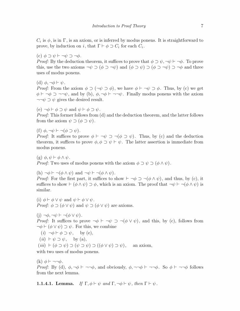
Introduction to Proof Theory 7
Ci is φ , is in Γ, is an axiom, or is inferred by modus ponens. It is straightforward toprove, by induction on i , that Γ ` φ ⊃ Ci for each Ci .
(c) φ ⊃ ψ ` ¬ψ ⊃ ¬φ .Proof: By the deduction theorem, it suffices to prove that φ ⊃ ψ,¬ψ ` ¬φ . To provethis, use the two axioms ¬ψ ⊃ (φ ⊃ ¬ψ) and (φ ⊃ ψ) ⊃ (φ ⊃ ¬ψ) ⊃ ¬φ and threeuses of modus ponens.
(d) φ,¬φ ` ψ .Proof: From the axiom φ ⊃ (¬ψ ⊃ φ), we have φ ` ¬ψ ⊃ φ . Thus, by (c) we getφ ` ¬φ ⊃ ¬¬ψ , and by (b), φ,¬φ ` ¬¬ψ . Finally modus ponens with the axiom¬¬ψ ⊃ ψ gives the desired result.
(e) ¬φ ` φ ⊃ ψ and ψ ` φ ⊃ ψ .Proof: This former follows from (d) and the deduction theorem, and the latter followsfrom the axiom ψ ⊃ (φ ⊃ ψ).
(f) φ,¬ψ ` ¬(φ ⊃ ψ).Proof: It suffices to prove φ ` ¬ψ ⊃ ¬(φ ⊃ ψ). Thus, by (c) and the deductiontheorem, it suffices to prove φ, φ ⊃ ψ ` ψ . The latter assertion is immediate frommodus ponens.
(g) φ, ψ ` φ ∧ ψ .Proof: Two uses of modus ponens with the axiom φ ⊃ ψ ⊃ (φ ∧ ψ).
(h) ¬φ ` ¬(φ ∧ ψ) and ¬ψ ` ¬(φ ∧ ψ).Proof: For the first part, it suffices to show ` ¬φ ⊃ ¬(φ ∧ ψ), and thus, by (c), itsuffices to show ` (φ ∧ ψ) ⊃ φ , which is an axiom. The proof that ¬ψ ` ¬(φ ∧ ψ) issimilar.
(i) φ ` φ ∨ ψ and ψ ` φ ∨ ψ .Proof: φ ⊃ (φ ∨ ψ) and ψ ⊃ (φ ∨ ψ) are axioms.
(j) ¬φ,¬ψ ` ¬(φ ∨ ψ).Proof: It suffices to prove ¬φ ` ¬ψ ⊃ ¬(φ ∨ ψ), and this, by (c), follows from¬φ ` (φ ∨ ψ) ⊃ ψ . For this, we combine
(i) ¬φ ` φ ⊃ ψ , by (e),
(ii) ` ψ ⊃ ψ , by (a),
(iii) ` (φ ⊃ ψ) ⊃ (ψ ⊃ ψ) ⊃ ((φ ∨ ψ) ⊃ ψ), an axiom,
with two uses of modus ponens.
(k) φ ` ¬¬φ .Proof: By (d), φ,¬φ ` ¬¬φ , and obviously, φ,¬¬φ ` ¬¬φ . So φ ` ¬¬φ followsfrom the next lemma.
1.1.4.1. Lemma. If Γ, φ ` ψ and Γ,¬φ ` ψ , then Γ ` ψ .

8 S. Buss
Proof. By (b) and (c), the two hypotheses imply that Γ ` ¬ψ ⊃ ¬φ and Γ ` ¬ψ ⊃¬¬φ . These plus the two axioms (¬ψ ⊃ ¬φ) ⊃ (¬ψ ⊃ ¬¬φ) ⊃ ¬¬ψ and ¬¬ψ ⊃ ψgive Γ ` ψ . 2
1.1.4.2. Lemma. Let the formula A involve only the propositional variables amongp1, . . . , pn . For 1 ≤ i ≤ n, suppose that Bi is either pi or ¬pi . Then, either
B1, . . . , Bn ` A or B1, . . . , Bn ` ¬A.
Proof. Define τ to be a truth assignment that makes each Bi true. By the soundnesstheorem, A (respectively, ¬A), can be proved from the hypotheses B1, . . . , Bn onlyif τ(A) = T (respectively τ(A) = F ). Lemma 1.1.4.2 asserts that the converse holdstoo.
The lemma is proved by induction on the complexity of A . In the base case,A is just pi : this case is trivial to prove since Bi is either pi or ¬pi . Now supposeA is a formula A1 ∨ A2 . If σ(A) = T , then we must have τ(Ai) = T for somei ∈ {1, 2} ; the induction hypothesis implies that B1, . . . , Bn ` Ai and thus, by (i)above, B1, . . . , Bn ` A . On the other hand, if τ(A) = F , then τ(A1) = τ(A2) = F ,so the induction hypothesis implies that B1, . . . , Bn ` ¬Ai for both i = 1 and i = 2.From this, (j) implies that B1, . . . , Bn ` ¬A . The cases where A has outermostconnective ∧ , ⊃ or ¬ are proved similarly. 2 .
We are now ready to complete the proof of the Completeness Theorem 1.1.3.Suppose A is a tautology. We claim that Lemma 1.1.4.2 can be strengthened to have
B1, . . . , Bk ` A
where, as before each Bi is either pi or ¬pi , but now 0 ≤ k ≤ n is permitted.We prove this by induction on k = n, n − 1, . . . , 1, 0. For k = n , this is justLemma 1.1.4.2. For the induction step, note that B1, . . . , Bk ` A follows fromB1, . . . , Bk, pk+1 ` A and B1, . . . , Bk,¬pk+1 ` A by Lemma 1.1.4.1. When k = 0,we have that ` A , which proves the Completeness Theorem.Q.E.D. Theorem 1.1.3
1.1.5. It still remains to prove the compactness theorem for propositional logic.This theorem states:
Compactness Theorem. Let Γ be a set of propositional formulas.
(1) Γ is satisfiable if and only if every finite subset of Γ is satisfiable.
(2) Γ ² A if and only if there is a finite subset Γ0 of Γ such that Γ0 ² A.
Since Γ ² A is equivalent to Γ∪{¬A} being unsatisfiable, (2) is implied by (1). It isfairly easy to prove the compactness theorem directly, and most introductory booksin mathematical logic present such a proof. Here, we shall instead, give a proof basedon the Tychonoff theorem; obviously this connection to topology is the reason for thename ‘compactness theorem.’

Introduction to Proof Theory 9
Proof. Let V be the set of propositional variables used in Γ; the sets Γ and Vneed not necessarily be countable. Let 2V denote the set of truth assignments on Vand endow 2V with the product topology by viewing it as the product of |V | copiesof the two element space with the discrete topology. That is to say, the subbasiselements of 2V are the sets Bp,i = {τ : τ(p) = i} for p ∈ V and i ∈ {T, F} . Notethat these subbasis elements are both open and closed. Recall that the Tychonofftheorem states that an arbitrary product of compact spaces is compact; in particular,2V is compact. (See Munkres [1975] for background material on topology.)
For φ ∈ Γ, define Dφ = {τ ∈ 2V : τ ² φ} . Since φ only involves finitely manyvariables, each Dφ is both open and closed. Now Γ is satisfiable if and only if ∩φ∈ΓDφ
is non-empty. By the compactness of 2V , the latter condition is equivalent to thesets ∩φ∈Γ0Dφ being non-empty for all finite Γ0 ⊂ Γ. This, in turn is equivalent toeach finite subset Γ0 of Γ being satisfiable. 2
The compactness theorem for first-order logic is more difficult; a purely model-theoretic proof can be given with ultrafilters (see, e.g., Eklof [1977]). We include aproof-theoretic proof of the compactness theorem for first-order logic for countablelanguages in section 2.3.7 below.
1.1.6. Remarks. There are of course a large number of possible ways to givesound and complete proof systems for propositional logic. The particular proofsystem F used above is adapted from Kleene [1952]. A more detailed proof of thecompleteness theorem for F and for related systems can be found in the textbookof Mendelson [1987]. The system F is an example of a class of proof systems calledFrege proof systems: a Frege proof system is any proof system in which all axioms andrules are schematic and which is implicationally sound and implicationally complete.Most of the commonly used proof systems similar to F are based on modus ponensas the only rule of inference; however, some (non-Frege) systems also incorporate aversion of the deduction theorem as a rule of inference. In these systems, if B hasbeen inferred from A , then the formula A ⊃ B may also be inferred. An exampleof such a system is the propositional fragment of the natural deduction proof systemdescribed in section 2.4.8 below.
Other rules of inference that are commonly allowed in propositional proof systemsinclude the substitution rule which allows any instance of φ to be inferred from φ , andthe extension rule which permits the introduction of abbreviations for long formulas.These two systems appear to be more powerful than Frege systems in that they seemto allow substantially shorter proofs of certain tautologies. However, whether theyactually are significantly more powerful than Frege systems is an open problem. Thisissues are discussed more fully by Pudlak in Chapter VIII.
There are several currently active areas of research in the proof theory of propo-sitional logic. Of course, the central open problem is the P versus NP question ofwhether there exists a polynomial time method of recognizing tautologies. Researchon the proof theory of propositional logic can be, roughly speaking, separated intothree problem areas. Firstly, the problem of “proof-search” is the question of

10 S. Buss
what are the best algorithmic methods for searching for propositional proofs. Theproof-search problem is important for artificial intelligence, for automated theoremproving and for logic programming. The most common propositional proof systemsused for proof-search algorithms are variations of the resolution system discussedin 1.3 below. A second, related research area is the question of proof lengths. Inthis area, the central questions concern the minimum lengths of proofs needed fortautologies in particular proof systems. This topic is treated in more depth inChapter VIII in this volume.
A third research area concerns the investigation of fragments of the propositionalproof system F . For example, propositional intuitionist logic is the logic whichis axiomatized by the system F without the axiom scheme ¬¬A ⊃ A . Anotherimportant example is linear logic. Brief discussions of these two logics can be foundin section 3.
1.2. The propositional sequent calculus
The sequent calculus, first introduced by Gentzen [1935] as an extension of his earliernatural deduction proof systems, is arguably the most elegant and flexible system forwriting proofs. In this section, the propositional sequent calculus for classical logicis developed; the extension to first-order logic is treated in 2.3 below.
1.2.1. Sequents and Cedents. In the Hilbert-style systems, each line in a proofis a formula; however, in sequent calculus proofs, each line in a proof is a sequent: asequent is written in the form
A1, . . . , Ak→B1, . . . , B`
where the symbol → is a new symbol called the sequent arrow (not to be confusedwith the implication symbol ⊃) and where each Ai and Bj is a formula. The intuitivemeaning of the sequent is that the conjunction of the Ai ’s implies the disjunction ofthe Bj ’s. Thus, a sequent is equivalent in meaning to the formula
k∧i=1
Ai ⊃∨j=1
Bj.
The symbols∧
and∨
represent conjunctions and disjunctions, respectively, of
multiple formulas. We adopt the convention that an empty conjunction (say, whenk = 0 above) has value “True”, and that an empty disjunction (say, when ` = 0above) has value “False”. Thus the sequent →A has the same meaning as theformula A , and the empty sequent → is false. A sequent is defined to be valid or atautology if and only if its corresponding formula is.
The sequence of formulas A1, . . . , Ak is called the antecedent of the sequentdisplayed above; B1, . . . , B` is called its succedent . They are both referred to ascedents.

Introduction to Proof Theory 11
1.2.2. Inferences and proofs. We now define the propositional sequent calculusproof system PK . A sequent calculus proof consists of a rooted tree (or sometimes adirected acyclic graph) in which the nodes are sequents. The root of the tree, writtenat the bottom, is called the endsequent and is the sequent proved by the proof. Theleaves, at the top of the tree, are called initial sequents or axioms. Usually, the onlyinitial sequents allowed are the logical axioms of the form A→A , where we furtherrequire that A be atomic.
Other than the initial sequents, each sequent in a PK-proof must be inferred byone of the rules of inference given below. A rule of inference is denoted by a figureS1
Sor S1 S2
Sindicating that the sequent S may be inferred from S1 or from the
pair S1 and S2 . The conclusion, S , is called the lower sequent of the inference; eachhypotheses is an upper sequent of the inference. The valid rules of inference for PKare as follows; they are essentially schematic, in that A and B denote arbitraryformulas and Γ, ∆, etc. denote arbitrary cedents.
Weak Structural Rules
Exchange:leftΓ, A,B, Π→∆Γ, B,A, Π→∆
Exchange:rightΓ→∆, A,B, ΛΓ→∆, B,A, Λ
Contraction:leftA,A, Γ→∆
A, Γ→∆Contraction:right
Γ→∆, A,AΓ→∆, A
Weakening:left Γ→∆A, Γ→∆
Weakening:right Γ→∆Γ→∆, A
The weak structural rules are also referred to as just weak inference rules. The restof the rules are called strong inference rules. The structural rules consist of the weakstructural rules and the cut rule.
The Cut RuleΓ→ ∆, A A, Γ→ ∆
Γ→ ∆
The Propositional Rules1
¬:leftΓ→∆, A
¬A, Γ→∆¬:right
A, Γ→∆Γ→∆,¬A
∧:leftA,B, Γ→∆
A ∧B, Γ→∆∧:right
Γ→∆, A Γ→∆, BΓ→∆, A ∧B
∨:leftA, Γ→∆ B, Γ→∆
A ∨B, Γ→∆∨:right
Γ→∆, A,BΓ→∆, A ∨B
⊃:leftΓ→∆, A B, Γ→∆
A ⊃ B, Γ→∆⊃:right
A, Γ→∆, BΓ→∆, A ⊃ B
1 We have stated the ∧ :left and the ∨ :right rules differently than the traditional form. Thetraditional definitions use the following two ∨ :right rules of inference

12 S. Buss
The above completes the definition of PK . We write PK ` Γ→∆ to denote thatthe sequent Γ→∆ has a PK-proof. When A is a formula, we write PK ` A tomean that PK ` →A .
The cut rule plays a special role in the sequent calculus, since, as is shown insection 1.2.8, the system PK is complete even without the cut rule; however, the useof the cut rule can significantly shorten proofs. A proof is said to be cut-free if doesnot contain any cut inferences.
1.2.3. Ancestors, descendents and the subformula property. All of theinferences of PK , with the exception of the cut rule, have a principal formula whichis, by definition, the formula occurring in the lower sequent of the inference which isnot in the cedents Γ or ∆ (or Π or Λ). The exchange inferences have two principalformulas. Every inference, except weakenings, has one or more auxiliary formulaswhich are the formulas A and B , occurring in the upper sequent(s) of the inference.The formulas which occur in the cedents Γ, ∆, Π or Λ are called side formulas of theinference. The two auxiliary formulas of a cut inference are called the cut formulas.
We now define the notions of descendents and ancestors of formulas occurring ina sequent calculus proof. First we define immediate descendents as follows: If C isa side formula in an upper sequent of an inference, say C is the i-th subformula ofa cedent Γ, Π, ∆ or Λ, then C ’s only immediate descendent is the correspondingoccurrence of the same formula in the same position in the same cedent in thelower sequent of the inference. If C is an auxiliary formula of any inference except anexchange or cut inference, then the principal formula of the inference is the immediatedescendent of C . For an exchange inference, the immediate descendent of the Aor B in the upper sequent is the A or B , respectively, in the lower sequent. Thecut formulas of a cut inference do not have immediate descendents. We say thatC is an immediate ancestor of D if and only if D is an immediate descendent of C .Note that the only formulas in a proof that do not have immediate ancestors are theformulas in initial sequents and the principal formulas of weakening inferences.
The ancestor relation is defined to be the reflexive, transitive closure of theimmediate ancestor relation; thus, C is an ancestor of D if and only if there is achain of zero or more immediate ancestors from D to C . A direct ancestor of D is anancestor C of D such that C is the same formula as D . The concepts of descendentand direct descendent are defined similarly as the converses of the ancestor and directancestor relations.
A simple, but important, observation is that if C is an ancestor of D , then C isa subformula of D . This immediately gives the following subformula property:
Γ→ ∆, A
Γ→ ∆, A ∨Band
Γ→ ∆, A
Γ→ ∆, B ∨A
and two dual rules of inference for ∧ :left. Our method has the advantage of reducing the numberof rules of inference, and also simplifying somewhat the upper bounds on cut-free proof length weobtain below.

Introduction to Proof Theory 13
1.2.4. Proposition. (The Subformula Property) If P is a cut-free PK-proof, thenevery formula occurring in P is a subformula of a formula in the endsequent of P .
1.2.5. Lengths of proofs. There are a number of ways to measure the lengthof a sequent calculus proof P ; most notably, one can measure either the number ofsymbols or the number of sequents occurring in P . Furthermore, one can requireP to be tree-like or to be dag-like; in the case of dag-like proofs no sequent needs tobe derived, or counted, twice. (‘Dag’ abbreviates ‘directed acyclic graph’, anothername for such proofs is ‘sequence-like’.)
For this chapter, we adopt the following conventions for measuring lengths ofsequent calculus proofs: proofs are always presumed to be tree-like, unless weexplicitly state otherwise, and we let ||P || denote the number of strong inferencesin a tree-like proof P . The value ||P || is polynomially related to the number ofsequents in P . If P has n sequents, then, of course, ||P || < n . On the other hand,it is not hard to prove that for any tree-like proof P of a sequent Γ→∆, there isa (still tree-like) proof of an endsequent Γ′→∆′ with at most ||P ||2 sequents andwith Γ′ ⊆ Γ and ∆′ ⊆ ∆. The reason we use ||P || instead of merely counting theactual number of sequents in P , is that using ||P || often makes bounds on proof sizesignificantly more elegant to state and prove.
Occasionally, we use ||P ||dag to denote the number of strong inferences in adag-like proof P .
1.2.6. Soundness Theorem. The propositional sequent calculus PK is sound.That is to say, any PK-provable sequent or formula is a tautology.
The soundness theorem is proved by observing that the rules of inference of PKpreserve the property of sequents being tautologies.
The implicational form of the soundness theorem also holds. If S is a set ofsequents, let an S-proof be any sequent calculus proof in which sequents from S arepermitted as initial sequents (in addition to the logical axioms). The implicationalsoundness theorem states that if a sequent Γ→∆ has an S-proof, then Γ→∆ ismade true by every truth assignment which satisfies S .
1.2.7. The inversion theorem. The inversion theorem is a kind of inverse tothe implicational soundness theorem, since it says that, for any inference exceptweakening inferences, if the conclusion of the inference is valid, then so are all of itshypotheses.
Theorem. Let I be a propositional inference, a cut inference, an exchange inferenceor a contraction inference. If I ’s lower sequent is valid, then so are are all of I ’supper sequents. Likewise, if I ’s lower sequent is true under a truth assignment τ ,then so are are all of I ’s upper sequents.
The inversion theorem is easily proved by checking the eight propositional inferencerules; it is obvious for exchange and contraction inferences.
14 S. Buss
Note that the inversion theorem can fail for weakening inferences. Most authorsdefine the ∧:left and ∨:right rules of inference differently than we defined themfor PK , and the inversion theorem can fail for these alternative formulations (see thefootnote on page 11).
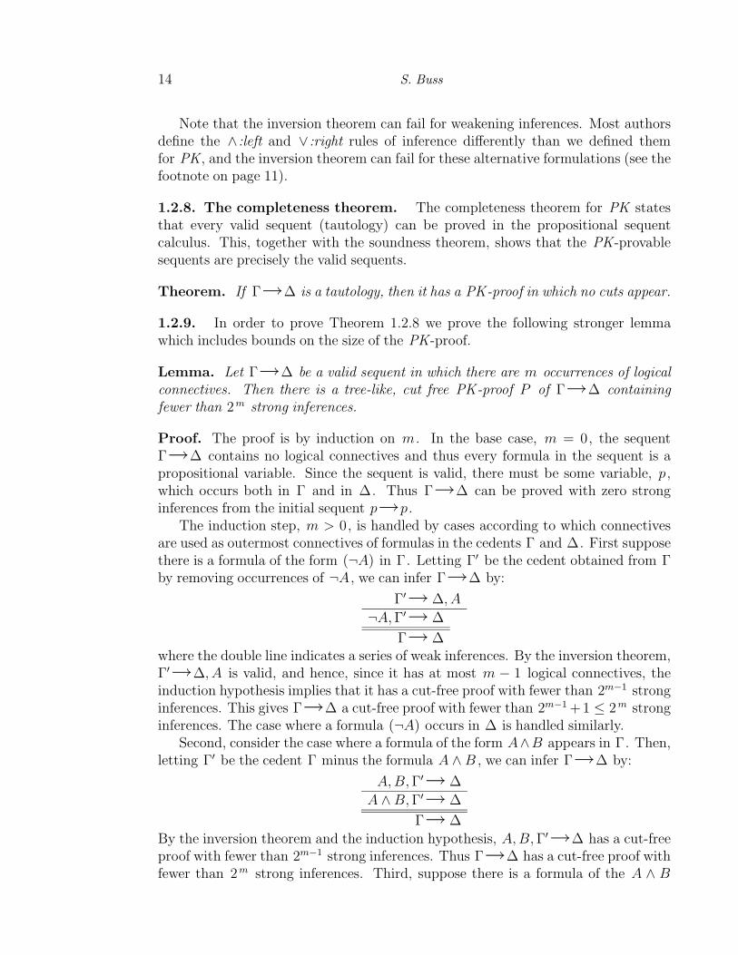
1.2.8. The completeness theorem. The completeness theorem for PK statesthat every valid sequent (tautology) can be proved in the propositional sequentcalculus. This, together with the soundness theorem, shows that the PK-provablesequents are precisely the valid sequents.
Theorem. If Γ→∆ is a tautology, then it has a PK-proof in which no cuts appear.
1.2.9. In order to prove Theorem 1.2.8 we prove the following stronger lemmawhich includes bounds on the size of the PK-proof.
Lemma. Let Γ→∆ be a valid sequent in which there are m occurrences of logicalconnectives. Then there is a tree-like, cut free PK-proof P of Γ→∆ containingfewer than 2m strong inferences.
Proof. The proof is by induction on m . In the base case, m = 0, the sequentΓ→∆ contains no logical connectives and thus every formula in the sequent is apropositional variable. Since the sequent is valid, there must be some variable, p ,which occurs both in Γ and in ∆. Thus Γ→∆ can be proved with zero stronginferences from the initial sequent p→p .
The induction step, m > 0, is handled by cases according to which connectivesare used as outermost connectives of formulas in the cedents Γ and ∆. First supposethere is a formula of the form (¬A) in Γ. Letting Γ′ be the cedent obtained from Γby removing occurrences of ¬A , we can infer Γ→∆ by:
Γ′→ ∆, A
¬A, Γ′→ ∆
Γ→ ∆where the double line indicates a series of weak inferences. By the inversion theorem,Γ′→∆, A is valid, and hence, since it has at most m − 1 logical connectives, theinduction hypothesis implies that it has a cut-free proof with fewer than 2m−1 stronginferences. This gives Γ→∆ a cut-free proof with fewer than 2m−1 +1 ≤ 2m stronginferences. The case where a formula (¬A) occurs in ∆ is handled similarly.
Second, consider the case where a formula of the form A∧B appears in Γ. Then,letting Γ′ be the cedent Γ minus the formula A ∧B , we can infer Γ→∆ by:
A,B, Γ′→ ∆
A ∧B, Γ′→ ∆
Γ→ ∆
By the inversion theorem and the induction hypothesis, A,B, Γ′→∆ has a cut-freeproof with fewer than 2m−1 strong inferences. Thus Γ→∆ has a cut-free proof withfewer than 2m strong inferences. Third, suppose there is a formula of the A ∧ B

Introduction to Proof Theory 15
appearing in the succedent ∆. Letting ∆′ be the the succedent ∆ minus the formulaA ∧B , we can infer
Γ→ ∆′, A Γ→ ∆′, BΓ→ ∆′, A ∧B
Γ→ ∆
By the inversion theorem, both of upper sequents above are valid. Furthermore, theyeach have fewer than m logical connectives, so by the induction hypothesis, theyhave cut-free proofs with fewer than 2m−1 strong inferences. This gives the sequentΓ→∆ a cut-free proof with fewer than 2m strong inferences.
The remaining cases are when a formula in the sequent Γ→∆ has outermostconnective ∨ or ⊃ . These are handled with the inversion theorem and the inductionhypothesis similarly to the above cases. 2
1.2.10. The bounds on the proof size in Lemma 1.2.9 can be improved somewhatby counting only the occurrences of distinct subformulas in Γ→∆. To makethis precise, we need to define the concepts of positively and negatively occurringsubformulas. Given a formula A , an occurrence of a subformula B of A , and aoccurrence of a logical connective α in A , we say that B is negatively bound by α ifeither (1) α is a negation sign, ¬ , and B is in its scope, or (2) α is an implication sign,⊃ , and B is a subformula of its first argument. Then, B is said to occur negatively(respectively, positively) in A if B is negatively bound by an odd (respectively, even)number of connectives in A . A subformula occurring in a sequent Γ→∆ is said tobe positively occurring if it occurs positively in ∆ or negatively in Γ; otherwise, itoccurs negatively in the sequent.
Lemma. Let Γ→∆ be a valid sequent. Let m′ equal the number of distinctsubformulas occurring positively in the sequent and m′′ equal the number of distinctsubformulas occurring negatively in the sequent. Let m = m′ + m′′ . Then there is atree-like, cut free PK-proof P containing fewer than 2m strong inferences.
Proof. (Sketch) Recall that the proof of Lemma 1.2.9 built a proof from the bottom-up, by choosing a formula in the endsequent to eliminate (i.e., to be inferred) andthereby reducing the total number of logical connectives and then appealing to theinduction hypothesis. The construction for the proof of the present lemma is exactlythe same, except that now care must be taken to reduce the total number of distinctpositively or negatively occurring subformulas, instead of just reducing the totalnumber of connectives. This is easily accomplished by always choosing a formulafrom the endsequent which contains a maximal number of connectives and which istherefore not a proper subformula of any other subformula in the endsequent. 2
1.2.11. The cut elimination theorem states that if a sequent has a PK-proof,then it has a cut-free proof. This is an immediate consequence of the soundnessand completeness theorems, since any PK-provable sequent must be valid, by thesoundness theorem, and hence has a cut-free proof, by the completeness theorem.

16 S. Buss
This is a rather slick method of proving the cut elimination theorem, but unfor-tunately, does not shed any light on how a given PK-proof can be constructivelytransformed into a cut-free proof. In section 2.3.7 below, we shall give a step-by-stepprocedure for converting first-order sequent calculus proofs into cut-free proofs; thesame methods work also for propositional sequent calculus proofs. We shall not,however, describe this constructive proof transformation procedure here; instead, wewill only state, without proof, the following upper bound on the increase in prooflength which can occur when a proof is transformed into a cut-free proof. (A proofcan be given using the methods of Sections 2.4.2 and 2.4.3.)
Cut-Elimination Theorem. Suppose P be a (possibly dag-like) PK-proof ofΓ→∆. Then Γ→∆ has a cut-free, tree-like PK-proof with less than or equalto 2||P ||dag strong inferences.
1.2.12. Free-cut elimination. Let S be a set of sequents and, as above, definean S-proof to be a sequent calculus proof which may contain sequents from S asinitial sequents, in addition to the logical sequents. If I is a cut inference occurringin an S-proof P , then we say I ’s cut formulas are directly descended from S if theyhave at least one direct ancestor which occurs as a formula in an initial sequent whichis in S . A cut I is said to be free if neither of I ’s auxiliary formulas is directlydescended from S . A proof is free-cut free if and only if it contains no free cuts. (SeeDefinition 2.4.4.1 for a better definition of free cuts.) The cut elimination theoremcan be generalized to show that the free-cut free fragment of the sequent calculus isimplicationally complete:
Free-cut Elimination Theorem. Let S be a sequent and S a set of sequents. IfS ² S, then there is a free-cut free S-proof of S .
We shall not prove this theorem here; instead, we prove the generalization of thisfor first-order logic in 2.4.4 below. This theorem is essentially due to Takeuti [1987]based on the cut elimination method of Gentzen [1935].
1.2.13. Some remarks. We have developed the sequent calculus only for classicalpropositional logic; however, one of the advantages of the sequent calculus is itsflexibility in being adapted for non-classical logics. For instance, propositionalintuitionistic logic can be formalized by a sequent calculus PJ which is definedexactly like PK except that succedents in the lower sequents of strong inferencesare restricted to contain at most one formula. As another example, minimal logicis formalized like PJ , except with the restriction that every succedent containexactly one formula. Linear logic, relevant logic, modal logics and others can also beformulated elegantly with the sequent calculus.
1.2.14. The Tait calculus. Tait [1968] gave a proof system similar in spirit to thesequent calculus. Tait’s proof system incorporates a number of simplifications withregard to the sequent calculus; namely, it uses sets of formulas in place of sequents,

Introduction to Proof Theory 17
it allows only propositional formulas to be negated, and there are no weak structuralrules at all.
Since the Tait calculus is often used for analyzing fragments of arithmetic, es-pecially in the framework of infinitary logic, we briefly describe it here. Formulasare built up from atomic formulas p , from negated atomic formulas ¬p , and withthe connectives ∧ and ∨ . A negated atomic formula is usually denoted p ; andthe negation operator is extended to all formulas by defining p to be just p , andinductively defining A ∨B and A ∧B to be A ∧B and A ∨B , respectively.
Frequently, the Tait calculus is used for infinitary logic. In this case, formulas
are defined so that whenever Γ is a set of formulas, then so are∨
Γ and∧
Γ. The
intended meaning of these formulas is the disjunction, or conjunction, respectively,of all the formulas in Γ.
Each line in a Tait calculus proof is a set Γ of formulas with the intended meaningof Γ being the disjunction of the formulas in Γ. A Tait calculus proof can be tree-likeor dag-like. The initial sets, or logical axioms, of a proof are sets of the form Γ∪{p, p} .In the infinitary setting, there are three rules of inference; namely,
Γ ∪ {Aj}Γ ∪ {
∨i∈I
Ai}where j ∈ I,
Γ ∪ {Aj : j ∈ I}Γ ∪ {
∧j∈I
Aj}(there are |I| many hypotheses), and
Γ ∪ {A} Γ ∪ {A}Γ
the cut rule.
In the finitary setting, the same rules of inference may also be used. It is evidentthat the Tait calculus is practically isomorphic to the sequent calculus. This isbecause a sequent Γ→∆ may be transformed into the equivalent set of formulascontaining the formulas from ∆ and the negations of the formulas from Γ. Theexchange and contraction rules are superfluous once one works with sets of formulas,the weakening rule of the sequent calculus is replaced by allowing axioms to containextra side formulas (this, in essence, means that weakenings are pushed up to theinitial sequents of the proof). The strong rules of inference for the sequent calculustranslate, by this means, to the rules of the Tait calculus.
Recall that we adopted the convention that the length of a sequent calculus proofis equal to the number of strong inferences in the proof. When we work with tree-likeproofs, this corresponds exactly to the number of inferences in the correspondingTait-style proof.
The cut elimination theorem for the (finitary) sequent calculus immediatelyimplies the cut elimination theorem for the Tait calculus for finitary logic; thisis commonly called the normalization theorem for Tait-style systems. For generalinfinitary logics, the cut elimination/normalization theorems may not hold; however,Lopez-Escobar [1965] has shown that the cut elimination theorem does hold forinfinitary logic with formulas of countably infinite length. Also, Chapters III and IV

18 S. Buss
of this volume discuss cut elimination in some infinitary logics corresponding totheories of arithmetic.
1.3. Propositional resolution refutations
The Hilbert-style and sequent calculus proof systems described earlier are quitepowerful; however, they have the disadvantage that it has so far proved to bevery difficult to implement computerized procedures to search for propositionalHilbert-style or sequent calculus proofs. Typically, a computerized procedure forproof search will start with a formula A for which a proof is desired, and willthen construct possible proofs of A by working backwards from the conclusion Atowards initial axioms. When cut-free proofs are being constructed this is fairlystraightforward, but cut-free proofs may be much longer than necessary and mayeven be too long to be feasibly constructed by a computer. General, non-cut-free,proofs may be quite short; however, the difficulty with proof search arises from theneed to determine what formulas make suitable cut formulas. For example, whentrying to construct a proof of Γ→∆ that ends with a cut inference; one has toconsider all formulas C and try to construct proofs of the sequents Γ→∆, C andC, Γ→∆. In practice, it has been impossible to choose cut formulas C effectivelyenough to effectively generate general proofs. A similar difficulty arises in trying toconstruct Hilbert-style proofs which must end with a modus ponens inference.
Thus to have a propositional proof system which would be amenable to comput-erized proof search, it is desirable to have a proof system in which (1) proof searchis efficient and does not require too many ‘arbitrary’ choices, and (2) proof lengthsare not excessively long. Of course, the latter requirement is intended to reflect theamount of available computer memory and time; thus proofs of many millions ofsteps might well be acceptable. Indeed, for computerized proof search, having aneasy-to-find proof which is millions of steps long may well be preferable to having ahard-to-find proof which has only hundreds of steps.
The principal propositional proof system which meets the above requirements isbased on resolution. As we shall see, the expressive power and implicational power ofresolution is weaker than that of the full propositional logic; in particular, resolutionis, in essence, restricted to formulas in conjunctive normal form. However, resolutionhas the advantage of being amenable to efficient proof search.
Propositional and first-order resolution were introduced in the influential workof Robinson [1965b] and Davis and Putnam [1960]. Propositional resolution proofsystems are discussed immediately below. A large part of the importance of proposi-tional resolution lies in the fact that it leads to efficient proof methods in first-orderlogic: first-order resolution is discussed in section 2.6 below.
1.3.1. Definition. A literal is defined to be either a propositional variable pi orthe negation of a propositional variable ¬pi . The literal ¬pi is also denoted pi ; and ifx is the literal pi , then x denotes the unnegated literal pi . The literal x is called the

Introduction to Proof Theory 19
complement of x . A positive literal is one which is an unnegated variable; a negativeliteral is one which is a negated variable.
A clause C is a finite set of literals. The intended meaning of C is the disjunctionof its members; thus, for σ a truth assignment, σ(C) equals True if and only ifσ(x) =True for some x ∈ C . Note that the empty clause, ∅ , always has value False.Since clauses that contain both x and x are always true, it is often assumed w.l.o.g.that no clause contains both x and x . A clause is defined to be positive (respectively,negative) if it contains only positive (resp., only negative) literals. The empty clauseis the only clause which is both positive and negative. A clause which is neitherpositive nor negative is said to be mixed.
A non-empty set Γ of clauses is used to represent the conjunction of its members.Thus σ(Γ) is True if and only if σ(C) is True for all C ∈ Γ. Obviously, the meaningof Γ is the same as the conjunctive normal form formula consisting of the conjunctionof the disjunctions of the clauses in Γ. A set of clauses is said to be satisfiable if thereis at least one truth assignment that makes it true.
Resolution proofs are used to prove that a set Γ of clauses is unsatisfiable: thisis done by using the resolution rule (defined below) to derive the empty clausefrom Γ. Since the empty clause is unsatisfiable this will be sufficient to show that Γis unsatisfiable.
1.3.2. Definition. Suppose that C and D are clauses and that x ∈ C and x ∈ Dare literals. The resolution rule applied to C and D is the inference
C D(C \ {x}) ∪ (D \ {x})
The conclusion (C \{x})∪ (D\{x}) is called the resolvent of C and D (with respectto x).2
Since the resolvent of C and D is satisfied by any truth assignment that satisfiesboth C and D , the resolution rule is sound in the following sense: if Γ is satisfiableand B is the resolvent of two clauses in Γ, then Γ ∪ {B} is satisfiable. Since theempty clause is not satisfiable, this yields the following definition of the resolutionproof system.
Definition. A resolution refutation of Γ is a sequence C1, C2, . . . , Ck of clauses suchthat each Ci is either in Γ or is inferred from earlier member of the sequence by theresolution rule, and such that Ck is the empty clause.
1.3.3. Resolution is defined to be a refutation procedure which refutes the satis-fiability of a set of clauses, but it also functions as a proof procedure for provingthe validity of propositional formulas; namely, to prove a formula A , one forms aset ΓA of clauses such that A is a tautology if and only if ΓA is unsatisfiable. Then
2Note that x is uniquely determined by C and D if we adopt the (optional) convention thatclauses never contain any literal and its complement.
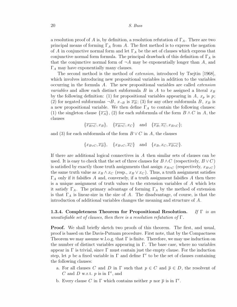
20 S. Buss
a resolution proof of A is, by definition, a resolution refutation of ΓA . There are twoprincipal means of forming ΓA from A . The first method is to express the negationof A in conjunctive normal form and let ΓA be the set of clauses which express thatconjunctive normal form formula. The principal drawback of this definition of ΓA isthat the conjunctive normal form of ¬A may be exponentially longer than A , andΓA may have exponentially many clauses.
The second method is the method of extension, introduced by Tsejtin [1968],which involves introducing new propositional variables in addition to the variablesoccurring in the formula A . The new propositional variables are called extensionvariables and allow each distinct subformula B in A to be assigned a literal xB
by the following definition: (1) for propositional variables appearing in A , xp is p ;(2) for negated subformulas ¬B , x¬B is xB ; (3) for any other subformula B , xB isa new propositional variable. We then define ΓA to contain the following clauses:(1) the singleton clause {xA} , (2) for each subformula of the form B ∧ C in A , theclauses
{xB∧C , xB}, {xB∧C , xC} and {xB, xC , xB∧C};and (3) for each subformula of the form B ∨ C in A , the clauses
{xB∨C , xB}, {xB∨C , xC} and {xB, xC , xB∨C}.
If there are additional logical connectives in A then similar sets of clauses can beused. It is easy to check that the set of three clauses for B ∧C (respectively, B ∨C )is satisfied by exactly those truth assignments that assign xB∧C (respectively, xB∨C )the same truth value as xB ∧ xC (resp., xB ∨ xC ). Thus, a truth assignment satisfiesΓA only if it falsifies A and, conversely, if a truth assignment falsifies A then thereis a unique assignment of truth values to the extension variables of A which letsit satisfy ΓA . The primary advantage of forming ΓA by the method of extensionis that ΓA is linear-size in the size of A . The disadvantage, of course, is that theintroduction of additional variables changes the meaning and structure of A .
1.3.4. Completeness Theorem for Propositional Resolution. If Γ is anunsatisfiable set of clauses, then there is a resolution refutation of Γ.
Proof. We shall briefly sketch two proofs of this theorem. The first, and usual,proof is based on the Davis-Putnam procedure. First note, that by the CompactnessTheorem we may assume w.l.o.g. that Γ is finite. Therefore, we may use induction onthe number of distinct variables appearing in Γ. The base case, where no variablesappear in Γ is trivial, since Γ must contain just the empty clause. For the inductionstep, let p be a fixed variable in Γ and define Γ′ to be the set of clauses containingthe following clauses:
a. For all clauses C and D in Γ such that p ∈ C and p ∈ D , the resolvent ofC and D w.r.t. p is in Γ′ , and
b. Every clause C in Γ which contains neither p nor p is in Γ′ .

Introduction to Proof Theory 21
Assuming, without loss of generality, that no clause in Γ contained both p and p , itis clear that the variable p does not occur in Γ′ . Now, it is not hard to show that Γ′
is satisfiable if and only if Γ is, from whence the theorem follows by the inductionhypothesis.
The second proof reduces resolution to the free-cut free sequent calculus. For this,if C is a clause, let ∆C be the cedent containing the variables which occur positivelyin C and ΠC be the variables which occur negatively in C . Then the sequentΠC→∆C is a sequent with no non-logical symbols which is identical in meaningto C . For example, if C = {p1, p2, p3} , then the associated sequent is p2→p1, p3 .Clearly, if C and D are clauses with a resolvent E , then the sequent ΠE→∆E isobtained from ΠC→∆C and ΠD→∆D with a single cut on the resolution variable.Now suppose Γ is unsatisfiable. By the completeness theorem for the free-cut freesequent calculus, there is a free-cut free proof of the empty sequent from the sequentsΠC→∆C with C ∈ Γ. Since the proof is free-cut free and there are no non-logicalsymbols appearing in any initial sequents, every cut formula in the proof must beatomic. Therefore no non-logical symbol appear anywhere in the proof and, byidentifying the sequents in the free-cut free proof with clauses and replacing each cutinference with the corresponding resolution inference, a resolution refutation of theempty clause is obtained. 2
1.3.5. Restricted forms of resolution. One of the principal advantages ofresolution is that it is easier for computers to search for resolution refutations thanto search for arbitrary Hilbert-style or sequent calculus proofs. The reason for thisis that resolution proofs are less powerful and more restricted than Hilbert-style andsequent calculus proofs and, in particular, there are fewer options on how to formresolution proofs. This explains the paradoxical situation that a less-powerful proofsystem can be preferable to a more powerful system. Thus it makes sense to considerfurther restrictions on resolution which may reduce the proof search space even more.Of course there is a tradeoff involved in using more restricted forms of resolution,since one may find that although restricted proofs are easier to search for, they area lot less plentiful. Often, however, the ease of proof search is more important thanthe existence of short proofs; in fact, it is sometimes even preferable to use a proofsystem which is not complete, provided its proofs are easy to find.
Although we do not discuss this until section 2.6, the second main advantage ofresolution is that propositional refutations can be ‘lifted’ to first-order refutations offirst-order formulas. It is important that the restricted forms of resolution discussednext also apply to first-order resolution refutations.
One example of a restricted form of resolution is implicit in the first proof of theCompleteness Theorem 1.3.4 based on the Davis-Putnam procedure; namely, for anyordering of the variables p1, . . . , pm , it can be required that a resolution refutationhas first resolutions with respect to p1 , then resolutions with respect to p2 , etc.,concluding with resolutions with respect to pm . This particular strategy is notparticularly useful since it does not reduce the search space sufficiently. We considernext several strategies that have been somewhat more useful.

22 S. Buss
1.3.5.1. Subsumption. A clause C is said to subsume a clause D if and only ifC ⊆ D . The subsumption principle states that if two clauses C and D have beenderived such that C subsumes D , then D should be discarded and not used furtherin the refutation. The subsumption principle is supported by the following theorem:
Theorem. If Γ is unsatisfiable and if C ⊂ D , then Γ′ = (Γ \ {D}) ∪ {C} is alsounsatisfiable. Furthermore, Γ′ has a resolution refutation which is no longer than theshortest refutation of Γ.
1.3.5.2. Positive resolution and hyperresolution. Robinson [1965a] intro-duced positive resolution and hyperresolution. A positive resolution inference is onein which one of the hypotheses is a positive clause. The completeness of positiveresolution is shown by:
Theorem. (Robinson [1965a]) If Γ is unsatisfiable, then Γ has a refutation contain-ing only positive resolution inferences.
Proof. (Sketch) It will suffice to show that it is impossible for an unsatisfiable Γ tobe closed under positive resolution inferences and not contain the empty clause. LetA be the set of positive clauses in Γ; A must be non-empty since Γ is unsatisfiable.Pick a truth assignment τ that satisfies all clauses in A and assigns the minimumpossible number of “true” values. Pick a clause L in Γ \ A which is falsified by τand has the minimum number of negative literals; and let p be one of the negativeliterals in L . Note that L exists since Γ is unsatisfiable and that τ(p) = True . Picka clause J ∈ A that contains p and has the rest of its members assigned false by τ ;such a clause J exists by the choice of τ . Considering the resolvent of J and L , weobtain a contradiction. 2
Positive resolution is nice in that it restricts the kinds of resolution refutations thatneed to be attempted; however, it is particularly important as the basis for hyperres-olution. The basic idea behind hyperresolution is that multiple positive resolutioninferences can be combined into a single inference with a positive conclusion. Tojustify hyperresolution, note that if R is a positive resolution refutation then theinferences in R can be uniquely partitioned into subproofs of the form
An
A3
A2
A1 B1
B2
B3
B4
. . .
Bn
An+1
where each of the clauses A1, . . . , An+1 are positive (and hence the clauses B1, . . . , Bn
are not positive). These n + 1 positive resolution inferences are combined into thesingle hyperresolution inference

Introduction to Proof Theory 23
A1 A2 A3 · · · An B1
An+1
(This construction is the definition of hyperresolution inferences.)
It follows immediately from the above theorem that hyperresolution is complete.The importance of hyperresolution lies in the fact that one can search for refutationscontaining only positive resolutions and that as clauses are derived, only the positiveclauses need to be saved for possible future use as hypotheses.
Negative resolution is defined similarly to positive resolution and is likewisecomplete.
1.3.5.3. Semantic resolution. Semantic resolution, independently introducedby Slagle [1967] and Luckham [1970], can be viewed as a generalization of positiveresolution. For semantic resolution, one uses a fixed truth assignment (interpreta-tion) τ to restrict the permissible resolution inferences. A resolution inference is saidto be τ -supported if one of its hypotheses is given value False by τ . Note that at mostone hypothesis can have value False, since the hypotheses contain complementaryoccurrences of the resolvent variable.
A resolution refutation is said to be τ -supported if each of its resolution inferencesare τ -supported. If τF is the truth assignment which assigns every variable the valueFalse, then a τF -supported resolution refutation is definitionally the same as apositive resolution refutation. Conversely, if Γ is a set of clauses and if τ is any truthassignment, then one can form a set Γ′ by complementing every variable in Γ whichhas τ -value True: clearly, a τ -supported resolution refutation of Γ is isomorphic toa positive resolution refutation of Γ′ . Thus, Theorem 1.3.5.2 is equivalent to thefollowing Completeness Theorem for semantic resolution:
Theorem. For any τ and Γ, Γ is unsatisfiable if and only if Γ has a τ -supportedresolution refutation.
It is possible to define semantic-hyperresolution in terms of semantic resolution, justas hyperresolution was defined in terms of positive resolution.
1.3.5.4. Set-of-support resolution. Wos, Robinson and Carson [1965] intro-duced set-of-support resolution as another principle for guiding a search for resolutionrefutations. Formally, set of support is defined as follows: if Γ is a set of clauses andif Π ⊂ Γ and Γ\Π is satisfiable, then Π is a set of support for Γ; a refutation R of Γis said to be supported by Π if every inference in R is derived (possibly indirectly)from at least one clause in Π. (An alternative, almost equivalent, definition wouldbe to require that no two members of Γ \ Π are resolved together.) The intuitiveidea behind set of support resolution is that when trying to refute Γ, one shouldconcentrate on trying to derive a contradiction from the part Π of Γ which is notknown to be consistent. For example, Γ \ Π might be a database of facts which ispresumed to be consistent, and Π a clause which we are trying to refute.

24 S. Buss
Theorem. If Γ is unsatisfiable and Π is a set of support for Γ, then Γ has arefutation supported by Π.
This theorem is immediate from Theorem 1.3.5.3. Let τ be any truth assignmentwhich satisfies Γ \ Π, then a τ -supported refutation is also supported by Π.
The main advantage of set of support resolution over semantic resolution is thatit does not require knowing or using a satisfying assignment for Γ \ Π.
1.3.5.5. Unit and input resolution. A unit clause is defined to be a clausecontaining a single literal; a unit resolution inference is an inference in at least oneof the hypotheses is a unit clause. As a general rule, it is desirable to perform unitresolutions whenever possible. If Γ contains a unit clause {x} , then by combiningunit resolutions with the subsumption principle, one can remove from Γ every clausewhich contains x and also every occurrence of x from the rest of the clauses in Γ.(The situation is a little more difficult when working in first-order logic, however.)This completely eliminates the literal x and reduces the number of and sizes ofclauses to consider.
A unit resolution refutation is a refutation which contains only unit resolutions.Unfortunately, unit resolution is not complete: for example, an unsatisfiable set Γwith no unit clauses cannot have a unit resolution refutation.
An input resolution refutation of Γ is defined to be a refutation of Γ in which everyresolution inference has at least one of its hypotheses in Γ. Obviously, a minimallength input refutation will be tree-like. Input resolution is also not complete; infact, it can refute exactly the same sets as unit resolution:
Theorem. (Chang [1970]) A set of clauses has a unit refutation if and only if it hasa input refutation.
1.3.5.6. Linear resolution. Linear resolution is a generalization of input resolu-tion which has the advantage of being complete: a linear resolution refutation of Γ isa refutation A1, A2, . . . , An−1, An = ∅ such that each Ai is either in Γ or is obtainedby resolution from Ai−1 and Aj for some j < i − 1. Thus a linear refutation hasthe same linear structure as an input resolution, but is allowed to reuse intermediateclauses which are not in Γ.
Theorem. (Loveland [1970] and Luckham [1970]) If Γ is unsatisfiable, then Γ hasa linear resolution refutation.
Linear and input resolution both lend themselves well to depth-first proof searchstrategies. Linear resolution is still complete when used in conjunction with set-of-support resolution.
Further reading. We have only covered some of the basic strategies for propositionresolution proof search. The original paper of Robinson [1965b] still provides anexcellent introduction to resolution; this and many other foundational papers on

Introduction to Proof Theory 25
this topic have been reprinted in Siekmann and Wrightson [1983]. In addition, thetextbooks by Chang and Lee [1973], Loveland [1978], and Wos et al. [1992] give amore complete description of various forms of resolution than we have given above.
Horn clauses. A Horn clause is a clause which contains at most one positive literal.Thus a Horn clause must be of the form {p, q1, . . . , qn} or of the form {q1, . . . , qn}with n ≥ 0. If a Horn clause is rewritten as sequents of atomic variables, it willhave at most one variable in the antecedent; typically, Horn clauses are written inreverse-sequent format so, for example, the two Horn clauses above would be writtenas implications
p ⇐ q1, . . . , qn
and
⇐ q1, . . . , qn.
In this reverse-sequent notation, the antecedent is written after the ⇐ , and thecommas are interpreted as conjunctions (∧ ’s). Horn clauses are of particular interestboth because they are expressive enough to handle many situations and becausedeciding the satisfiability of sets of Horn clauses is more feasible than deciding thesatisfiability of arbitrary sets of clauses. For these reasons, many logic programmingenvironments such as PROLOG are based partly on Horn clause logic.
In propositional logic, it is an easy matter to decide the satisfiability of a setof Horn clauses; the most straightforward method is to restrict oneself to positiveunit resolution. A positive unit inference is a resolution inference in which one ofthe hypotheses is a unit clause containing a positive literal only. A positive unitrefutation is a refutation containing only positive unit resolution inferences.
Theorem. A set of Horn clauses is unsatisfiable if and only if it has a positive unitresolution refutation.
Proof. Let Γ be an unsatisfiable set of Horn clauses. Γ must contain at least onepositive unit clause {p} , since otherwise the truth assignment that assigned False toall variables would satisfy Γ. By resolving {p} against all clauses containing p , andthen discarding all clauses which contain p or p , one obtains a smaller unsatisfiableset of Horn clauses. Iterating this yields the desired positive unit refutation. 2
Positive unit resolutions are quite adequate in propositional logic, however, theydo not lift well to applications in first-order logic and logic programming. Forthis, a more useful method of search for refutations is based on combining semanticresolution, linear resolution and set-of-support resolution:
1.3.5.7. Theorem. Henschen and Wos [1974]. Suppose Γ is an unsatisfiable setof Horn clauses with Π ⊆ Γ a set of support for Γ, and suppose that every clausein Γ \ Π contains a positive literal. Then Γ has a refutation which is simultaneouslya negative resolution refutation and a linear refutation and which is supported by Π.

26 S. Buss
Note that the condition that every clause in Γ \ Π contains a positive literal meansthat the truth assignment τ that assigns True to every variable satisfies Γ \Π. Thusa negative resolution refutation is the same as a τ -supported refutation and hence issupported by Π.
The theorem is fairly straightforward to prove, and we leave the details to thereader. However, note that since every clause in Γ \ Π is presumed to contain apositive literal, it is impossible to get rid of all positive literals only by resolvingagainst clauses in Γ \ Π. Therefore, Π must contain a negative clause C such thatthere is a linear derivation that begins with C , always resolves against clauses in Γ\Πyielding negative clauses only, and ending with the empty clause. The resolutionrefutations of Theorem 1.3.5.7, or rather the lifting of these to Horn clauses describedin section 2.6.5, can be combined with restrictions on the order in which literals areresolved to give what is commonly called SLD-resolution.
2. Proof theory of first-order logic
2.1. Syntax and semantics
2.1.1. Syntax of first-order logic. First-order logic is a substantial extensionof propositional logic, and allows reasoning about individuals using functions andpredicates that act on individuals. The symbols allowed in first-order formulasinclude the propositional connectives, quantifiers, variables, function symbols, con-stant symbols and relation symbols. We take ¬ , ∧ , ∨ and ⊃ as the allowedpropositional connectives. There is an infinite set of variable symbols; we usex, y, z, . . . and a, b, c, . . . as metasymbols for variables. The quantifiers are theexistential quantifiers, (∃x), and the universal quantifiers, (∀x), which mean “thereexists x” and “for all x”. A given first-order language contains a set of functionsymbols of specified arities, denoted by metasymbols f, g, h, . . . and a set of relationsymbols of specified arities, denoted by metasymbols P,Q,R, . . . . Function symbolsof arity zero are called constant symbols. Sometimes the first-order language containsa distinguished two-place relation symbol = for equality.
The formulas of first-order logic are defined as follows. Firstly, terms are built upfrom function symbols, constant symbols and variables. Thus, any variable x is aterm, and if t1, . . . , tk are terms and f is k -ary, then f(t1, . . . , tk) is a term. Second,atomic formulas are defined to be of the form P (t1, . . . , tk) for P a k -ary relationsymbol. Finally, formulas are inductively to be built up from atomic formulas andlogical connectives; namely, any atomic formula is a formula, and if A and B areformulas, then so are (¬A), (A∧B), (A∨B), (A ⊃ B), (∀x)A and (∃x)A . To avoidwriting too many parentheses, we adopt the conventions on omitting parentheses inpropositional logic with the additional convention that quantifiers bind more tightlythan binary propositional connectives. In addition, binary predicate symbols, suchas = and < , are frequently written in infix notation.
Consider the formula (x = 0∨ (∀x)(x 6= f(x))). (We use x 6= f(x) to abbreviate(¬x = f(x)).) This formula uses the variable x in two different ways: on one hand, it

Introduction to Proof Theory 27
asserts something about an object x ; and on the other hand, it (re)uses the variable xto state a general property about all objects. Obviously it would be less confusing towrite instead (x = 0 ∨ (∀y)(y 6= f(y))); however, there is nothing wrong, formallyspeaking, with using x in two ways in the same formula. To keep track of this, weneed to define free and bound occurrences of variables. An occurrence of a variable xin a formula A is defined to be any place that the symbol x occurs in A , except inquantifer symbols (Qx). (We write (Qx) to mean either (∀x) or (∃x).) If (Qx)(· · ·)is a subformula of A , then the scope of this occurrence of (Qx) is defined to be thesubformula denoted (· · ·). An occurrence of x in A is said to be bound if and only ifit is in the scope of a quantifier (Qx); otherwise the occurrence of x is called free. Ifx is a bound occurrence, it is bound by the rightmost quantifier (Qx) which it is inthe scope of. A formula in which no variables appear freely is called a sentence.
The intuitive idea of free occurrences of variables in A is that A says somethingabout the free variables. If t is a term, we define the substitution of t for x in A ,denoted A(t/x) to be the formula obtained from A by replacing each free occurrenceof x in A by the term t . To avoid unwanted effects, we generally want t to befreely substitutable for x , which means that no free variable in t becomes boundin A as a result of this substitution; formally defined, this means that no freeoccurrence of x in A occurs in the scope of a quantifier (Qy) with y a variableoccurring in t . The simultaneous substitution of t1, . . . , tk for x1, . . . , xk in A ,denoted A(t1/x1, . . . , tk/xk), is defined similarly in the obvious way.
To simplify notation, we adopt some conventions for denoting substitution.Firstly, if we write A(x) and A(t) in the same context, this indicates that A = A(x)is a formula, and that A(t) is A(t/x). Secondly, if we write A(s) and A(t) in thesame context, this is to mean that A is formula, x is some variable, and that A(s) isA(s/x) and A(t) is A(t/x).
The sequent calculus, discussed in 2.3, has different conventions on variables thanthe Hilbert-style systems discussed in 2.2; most notably, it has distinct classes ofsymbols for free variables and bound variables. See section 2.3.1 for the discussion ofthe usage of variables in the sequent calculus.
2.1.2. Semantics of first-order logic. In this section, we define the semantics,or ‘meaning’, of first-order formulas. Since this is really model theory instead of prooftheory, and since the semantics of first-order logic is well-covered in any introductorytextbook on mathematical logic, we give only a very concise description of thenotation and conventions used in this chapter.
In order to ascribe a truth value to a formula, it is necessary to give an interpre-tation of the non-logical symbols appearing in it; namely, we must specify a domainor universe of objects, and we must assign meanings to each variable occurringfreely and to each function symbol and relation symbol appearing in the formula. Astructure M (also called an interpretation), for a given language L , consists of thefollowing:
(1) A non-empty universe M of objects, intended to be the universe of objects overwhich variables and terms range;

28 S. Buss
(2) For each k -ary function f of the language, an interpretation fM : Mk 7→ M ;and
(3) For each k -ary relation symbol P of the language, an interpretation PM ⊆ Mk
containing all k -tuples for which P is intended to hold. If the first-orderlanguage contains the symbol for equality, then =M must be the true equalitypredicate on M .
We shall next define the true/false value of a sentence in a structure. This is possiblesince the structure specifies the meaning of all the function symbols and relationsymbols in the formula, and the quantifiers and propositional connectives take theirusual meanings. For A a sentence and M a structure, we write M ² A to denoteA being true in the structure M . In this case, we say that M is a model of A , orthat A is satisfied by M . Often, we wish to talk about the meaning of a formula Ain which free variables occur. For this, we need not only a structure, but also anobject assignment, which is a mapping σ from the set of variables (at least the onesfree in A) to the universe M . The object assignment σ gives meanings to the freelyoccurring variables, and it is straightforward to define the property of A being truein a given structure M under a given object assignment σ , denoted M ² A[σ] .
To give the formal definition of M ² A[σ] , we first need to define the interpre-tation of terms, i.e, we need to formally define the manner in which arbitrary termsrepresent objects in the universe M . To this end, we define tM[σ] by induction onthe complexity of t . For x a variable, xM[σ] is just σ(x). For t a term of the formf(t1, . . . , tk), we define tM[σ] to equal fM(tM1 [σ], . . . , tMk [σ]). If t is a closed term,i.e., contains no variables, then tM[σ] is independent of σ and is denoted by just tM .
If σ is an object assignment and m ∈ M , then σ(m/x) is the object assignmentwhich is identical to σ except that it maps x to m . We are now ready to definethe truth of A in M with respect to σ , by induction on the complexity of A . ForA an atomic formula P (t1, . . . , tk), then M ² A[σ] holds if and only if the k -tuple(tM1 [σ], . . . , tMk [σ]) is in PM . Also, M ² ¬A[σ] holds if and only M 2 A[σ] , where2 is the negation of ² . Likewise, the value of M ² A ¯ B[σ] with ¯ one of thebinary propositional connectives depends only on the truth values of M ² A[σ]and M ² B[σ] , in the obvious way according to Table 1 above. If A is (Qx)Bwith Q denoting either ∃ or ∀ , then M ² A[σ] holds if and only if the propertyM ² B[σ(m/x)] holds for some (respectively, for all) m ∈ M .
We say that a formula A is valid in M , if M ² A[σ] holds for all appropriateobject assignments. A formula is defined to be valid if and only if it is valid in allstructures. If Γ is a set of formulas, we say Γ is valid in M , written M ² Γ, if andonly if every formula in Γ is valid in M . When M ² Γ, we say that Γ is satisfiedby M . The set Γ is satisfiable if and only if it is satisfied by some model.
For Γ a set of formulas and A a formula, we define Γ logically implies A , Γ ² A ,to hold if A is valid in every structure in which Γ is valid. If Γ is the empty set, wewrite just ² A , which means of course that A is valid.3
3This definition of Γ ² A has the slightly unexpected result that free variables appearing in Γare treated as if they are universally quantified. For example, according to our definition, we have

Introduction to Proof Theory 29
2.1.3. For languages which contain the equality symbol, =, the interpretation of=M in any structure M must be true equality. Of course, this restriction influencesthe definition of Γ ² A in languages which contain equality. Let ²′ indicate logicalimplication defined with respect to all structures, including structures in whichequality is not interpreted by true equality. It is an elementary, but important, factthat ² can be defined in terms of ²′ . Namely, let EQ be the set of equality axiomsdefined in section 2.2.1 below; then Γ ² A holds if and only if Γ, EQ ²′ A holds.
2.1.4. Definition. A first-order theory is a set T of sentences closed under logicalimplication; i.e., if T ² A then A ∈ T . An axiomatization of T is a set Γ of sentencessuch that T is precisely the set of sentences logically implied by Γ.
2.2. Hilbert-style proof systems
2.2.1. A proof system. We give here an example of a proof system FFO forfirst-order logic, which is an extension of F to first-order logic. In addition to theaxioms of F and the rule modus ponens, there are two axiom schemes:
A(t) ⊃ (∃x)A(x) and (∀x)A(x) ⊃ A(t)
where A may be any formula and t any term. There are also two quantifier rules ofinference:
C ⊃ A(x)
C ⊃ (∀x)A(x)and
A(x) ⊃ C
(∃x)A(x) ⊃ C
where, in both inferences, x may not appear freely in C .If the first-order language under consideration contains the distinguished equality
sign (=), then the equality axioms must also be included; namely,
(∀x)(x = x)
(∀~x)(∀~y)(x1 = y1 ∧ · · · ∧ xk = yk ⊃ f(~x) = f(~y))
(∀~x)(∀~y)(x1 = y1 ∧ · · · ∧ xk = yk ∧ P (~x) ⊃ P (~y))
where f and P are arbitrary function and predicate symbols and k is their arity.We leave it to the reader to check that the symmetry and transitivity of equality
follow from these axioms, since in the third equality axiom, P may be the equalitysign. We write FFO ` A to denote A having an FFO -proof.
A(x) ² (∀x)A(x), and thus A(x) ² A(y). An alternative definition of logical implication is oftenused (but not in this chapter!) in which free variables occurring in Γ are treated as syntacticallyas constants; under this definition A(x) ² (∀x)A(x) does not hold in general.
The advantage our choice for the definition of ² , is that it yields a simpler and more elegantproof-theory. This choice does not involve any loss of expressive power since, instead of freevariables in Γ, one can use new constant symbols, and thus obtain the same effect as thealternative definition of ² . In any event, the two definitions of ² coincide when Γ is a set ofsentences.

30 S. Buss
2.2.2. The Soundness Theorem.
(1) If FFO ` A, then ² A.
(2) Let Γ be a set of sentences. If there is an FFO -proof of A using sentences fromΓ as additional axioms, then Γ ² A.
The Soundness Theorem states that FFO proves only valid formulas. Both partsof the soundness theorem are readily proved by induction on the number of lines ina proof.
2.2.3. The Completeness Theorem.
(1) If ² A, then FFO ` A.
(2) Let Γ be a set of formulas. If Γ ² A, then there is an FFO -proof of A usingsentences from Γ as additional axioms.
The completeness theorem and soundness theorem together show that FFO is anadequate system for formalizing first-order logic. The completeness theorem wasproved originally by Godel [1930]; the now-standard textbook proof is due to Henkin[1949]. We shall not give a proof for the completeness of FFO here; instead, weshall prove the completeness of the cut-free fragment of LK in 2.3.7 below. It isstraightforward to see that FFO can simulate the LK proof system, and this givesan indirect proof of the completeness of FFO .
2.2.4. A set Γ of sentences is consistent if and only if there is no sentence A suchthat both A and ¬A are provable from Γ and, equivalently, if and only if thereis some formula A such that there is no proof of A from Γ. The soundness andcompleteness theorems immediately imply that Γ is consistent if and only if Γ issatisfiable.
2.2.5. Historical remarks. Frege [1879] gave the first full formulation of first-order logic. Frege used a pictorial representation of propositional connectives andquantifiers; one remnant of his notation that is still in use is “` A”, which was Frege’snotation for “A is asserted to be true”. Frege used the pictorial notation A
to express a proposition A ; whereas he used the notation A to express theassertion that the proposition A is true (or has been proved). Negation, implication,and universal quantification were represented by Frege with pictures such as
A , AB
and §¦x A ,
which represent the propositions ¬A , B ⊃ A , and (∀x)A , respectively. Theseconstructions can be iterated to form arbitrary first-order expression; that is to say,in the pictures above, A and B may be replaced by arbitrary pictorial propositions.The addition of a vertical line to the left end of a proposition indicates that theproposition has been established to be true (e.g., proved). Thus, for instance

Introduction to Proof Theory 31
§¦x AB and §¦x A
B
denote the proposition B ⊃ (∃x)A and the assertion that this proposition has beenestablished, respectively.
Frege also developed extensions to his first-order logic to include functionals andpredicates; however, these extensions were later discovered by Russell to introduceset-theoretic paradoxes.
Peano [1889] introduced, independently of Frege, a fragment of first-order logicfor reasoning about integers. Based on the work of Frege and Peano, Whiteheadand Russell [1910] gave a consistent framework for formalizing mathematics basedon first-order logic, using universal and existential quantifiers denoted (x) and (∃x).
The ‘Hilbert-style’ system given above is apparently so-named because it is closelyrelated to a system used by Hilbert and Ackermann [1928], which is based on earlierlectures of Hilbert. The later work of Hilbert and Bernays [1934-39], however,used the ε-calculus instead of a ‘Hilbert-style’ system. The ε-calculus contains noquantifiers, but in their place uses symbols εx(A(x)) which are intended to denotean object x such that A(x) holds, if there is such an object. Note that other freevariables and other uses of ε symbols may appear in A(x). The ε-symbol can beused to express quantifiers by the informal equivalences (∃x)A(x) ⇔ A(εx(A(x)))and (∀x)A(x) ⇔ A(εx(¬A(x))).
The Hilbert-style system we used above is essentially that of Kleene [1952].
2.3. The first-order sequent calculus
In this section, the propositional sequent calculus, introduced in section 1.2, isenlarged to a proof system for first-order logic.
2.3.1. Free and bound variables. The first-order sequent calculus has twoclasses of variables, called free variables and bound variables. There are infinitelymany variables of each type; free variables are denoted by the metavariablesa, b, c, . . . , and bound variables by the metavariables z, y, x, . . . . The essential idea isthat free variables may not be quantified, while bound variables may not occur freelyin formulas. The syntactic distinction between free and bound variables necessitatesa change to the definitions of terms and formulas. Firstly, terms are now definedas being built up from free variables and function symbols; whereas, the semitermsare defined as being built up from free and bound variables and function symbols.Secondly, only bound variables may ever be quantified. The set of formulas is nowredefined with the additional requirement that only free variables may occur freelyin formulas. Semiformulas are like formulas, except that bound variables may occurfreely in semiformulas. We henceforth use r, s, t, . . . as metavariables for terms, andA,B,C, . . . as metavariables for formulas.
Note that in general, a subformula of a formula will be a semiformula instead ofa formula.
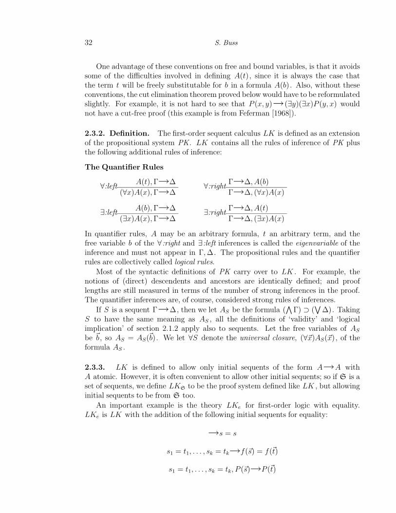
32 S. Buss
One advantage of these conventions on free and bound variables, is that it avoidssome of the difficulties involved in defining A(t), since it is always the case thatthe term t will be freely substitutable for b in a formula A(b). Also, without theseconventions, the cut elimination theorem proved below would have to be reformulatedslightly. For example, it is not hard to see that P (x, y)→(∃y)(∃x)P (y, x) wouldnot have a cut-free proof (this example is from Feferman [1968]).
2.3.2. Definition. The first-order sequent calculus LK is defined as an extensionof the propositional system PK . LK contains all the rules of inference of PK plusthe following additional rules of inference:
The Quantifier Rules
∀:left A(t), Γ→∆
(∀x)A(x), Γ→∆∀:right Γ→∆, A(b)
Γ→∆, (∀x)A(x)
∃:left A(b), Γ→∆
(∃x)A(x), Γ→∆∃:right Γ→∆, A(t)
Γ→∆, (∃x)A(x)
In quantifier rules, A may be an arbitrary formula, t an arbitrary term, and thefree variable b of the ∀:right and ∃:left inferences is called the eigenvariable of theinference and must not appear in Γ, ∆. The propositional rules and the quantifierrules are collectively called logical rules.
Most of the syntactic definitions of PK carry over to LK . For example, thenotions of (direct) descendents and ancestors are identically defined; and prooflengths are still measured in terms of the number of strong inferences in the proof.The quantifier inferences are, of course, considered strong rules of inferences.
If S is a sequent Γ→∆, then we let AS be the formula (∧
Γ) ⊃ (∨
∆). TakingS to have the same meaning as AS , all the definitions of ‘validity’ and ‘logicalimplication’ of section 2.1.2 apply also to sequents. Let the free variables of AS
be ~b , so AS = AS(~b). We let ∀S denote the universal closure, (∀~x)AS(~x), of theformula AS .
2.3.3. LK is defined to allow only initial sequents of the form A→A withA atomic. However, it is often convenient to allow other initial sequents; so if S is aset of sequents, we define LKS to be the proof system defined like LK , but allowinginitial sequents to be from S too.
An important example is the theory LKe for first-order logic with equality.LKe is LK with the addition of the following initial sequents for equality:
→s = s
s1 = t1, . . . , sk = tk→f(~s) = f(~t)
s1 = t1, . . . , sk = tk, P (~s)→P (~t)
Introduction to Proof Theory 33
We say that a set S is closed under substitution, if whenever Γ(a)→∆(a) isin S and t is a term, then Γ(t)→∆(t) is also in S .
2.3.4. When P is a proof, we write P (a) and P (t) to indicate that P (t) is theresult of replacing every free occurrence of a in formulas of P with t .
Theorem. Let S be a set of sequents which is closed under substitution. If P (b)is an LKS-proof, and if neither b nor any variable in t is used as an eigenvariablein P (b), then P (t) is a valid LKS-proof.
2.3.5. Definition. A free variable in the endsequent of a proof is called a parametervariable of the proof. A proof P is said to be in free variable normal form providedthat (1) no parameter variable is used as an eigenvariable, and (2) every other freevariable appearing in P is used exactly once as an eigenvariable and appears in Ponly in sequents above the inference for which it is used as an eigenvariable.
In this chapter, we consider only tree-like proofs and thus any proof may be put infree variable normal form by merely renaming variables.
2.3.6. Soundness Theorem. Let Γ→∆ be an arbitrary sequent.
(1) If Γ→∆ has an LK -proof, then Γ→∆ is valid.
(2) Let S be a set of sequents. If Γ→∆ has an LKS-proof, then S ² Γ→∆.
The soundness theorem is readily proved by induction on the number of inferencesin a proof.
2.3.7. Completeness of cut-free LK . We next prove the completeness of thecut-free fragment of LK and, more generally, the completeness of LKS. Since ourproofs of completeness also give a proof of the (countable) compactness theorem, weinclude the compactness theorem as part (2) of the completeness theorem.
Cut-free Completeness Theorem. Let Γ→∆ be a sequent in a first-order lan-guage L which does not contain equality.
(1) If Γ→∆ is valid, then it has a cut-free LK -proof.
(2) Let Π be a set of sentences. If Π logically implies Γ→∆, then there areC1, . . . , Ck ∈ Π such that C1, . . . , Ck, Γ→∆ has a cut-free LK -proof.
Corollary. Let S be a set of sequents. If S logically implies Γ→∆, then Γ→∆has an LKS-proof.
Note that in the corollary, the LKS-proof may not be cut-free. An important specialcase of the corollary is that LKe is complete. Although, in general, the cut-freefragment of LKS may not be complete; we shall see later that it is always possibleto get LKS proofs which contain no ‘free cuts’.

34 S. Buss
The corollary is an immediate consequence of the cut-free completeness theorem.This is because, if S ² Γ→∆, then part (2) of the theorem implies that there areS1, . . . , Sk ∈ S so that ∀S1, . . . ,∀Sk, Γ→∆ has an LK -proof. But clearly each→∀Si has an LKS-proof, so with k further cut inferences, Γ→∆ also has anLKS-proof.
Proof. Part (2) of the cut-free completeness theorem clearly implies part (1); weshall prove (2) only for the case where Π is countable (and hence the language L is,w.l.o.g., countable). Assume Π logically implies Γ→∆. The general idea of theargument is to try to build an LK -proof of Γ→∆ from the bottom up, workingbackwards from Γ→∆ to initial sequents. This is, of course, analogous to theprocedure used to prove Theorem 1.2.8; but because of the presence of quantifiers,the process of searching for a proof of Γ→∆ is no longer finite. Thus, we shallhave to show the proof-search process eventually terminates — this will be done byshowing that if the proof-search does not yield a proof, then Γ→∆ is not valid.
Since the language is countable, we may enumerate all L-formulas asA1, A2, A3, . . . so that every L-formula occurs infinitely often in the enumeration.Likewise, we enumerate all L-terms as t1, t2, t3, . . . with each term repeated infinitelyoften. We shall attempt to construct a cut-free proof P of Γ→∆. The constructionof P will proceed in stages: initially, P consists of just the sequent Γ→∆; ateach stage, P will be modified (we keep the same name P for the new partiallyconstructed P ). A sequent in P is said to be active provided it is a leaf sequent of Pand there is no formula that occurs in both its antecedent and its succedent. Notethat a non-active leaf sequent is derivable with a cut-free proof.
We enumerate all pairs 〈Ai, tj〉 by a diagonal enumeration; each stage of theconstruction of P considers one such pair. Initially, P is the single sequent Γ→∆.At each stage we do the following:
Loop: Let 〈Ai, tj〉 be the next pair in the enumeration.
Step (1): If Ai is in Π, then replace every sequent Γ′→∆′ in P with the sequentΓ′, Ai→∆′ .
Step (2): If Ai is atomic, do nothing and proceed to the next stage. Otherwise,we will modify P at the active sequents which contain Ai by doing one ofthe following:
Case (2a): If Ai is ¬B , then every active sequent in P which contains Ai , sayof form Γ′,¬B, Γ′′→∆′ , is replaced by the derivation
Γ′,¬B, Γ′′→ ∆′, B
Γ′,¬B, Γ′′→ ∆′
and similarly, every active sequent in P of the form Γ′→∆′,¬B, ∆′′ isreplaced by the derivation
B, Γ′→ ∆′,¬B, ∆′′
Γ′→ ∆′,¬B, ∆′′

Introduction to Proof Theory 35
Case (2b): If Ai is of the form B ∨ C , then every active sequent in P of theform Γ′, B ∨ C, Γ′′→∆′ , is replaced by the derivation
B, Γ′, B ∨ C, Γ′′→ ∆′ C, Γ′, B ∨ C, Γ′′→ ∆′
Γ′, B ∨ C, Γ′′→ ∆′
And, every active sequent in P of the form Γ′→∆′, B ∨C, ∆′′ is replacedby the derivation
Γ′→ ∆′, B ∨ C, ∆′′, B, C
Γ′→ ∆′, B ∨ C, ∆′′
Cases (2c)-(2d): The cases where Ai has outermost connective ⊃ or ∧ aresimilar (dual) to case (2b), and are omitted here.
Case (2e): If Ai is of the form (∃x)B(x), then every active sequent in P of theform Γ′, (∃x)B(x), Γ′′→∆′ is replaced by the derivation
B(c), Γ′, (∃x)B(x), Γ′′→ ∆′
Γ′, (∃x)B(x), Γ′′→ ∆′
where c is a new free variable, not used in P yet. In addition, any activesequent of the form Γ′→∆′, (∃x)B(x), ∆′′ is replaced by the derivation
Γ′→ ∆′, (∃x)B(x), ∆′′, B(tj)
Γ′→ ∆′, (∃x)B(x), ∆′′
Note that this, and the dual ∀:left case, are the only cases where tj is used.These two cases are also the only two cases where it is really necessary tokeep the formula Ai in the new active sequent; we have however, alwayskept Ai since it makes our arguments a little simpler.
Case (2f): The case where Ai begins with a universal quantifier is dual tocase (2e).
Step (3): If there are no active sequents remaining in P , exit from the loop;otherwise, continue with the next loop iteration.
End loop.
If the algorithm constructing P ever halts, then P gives a cut-free proof ofC1, . . . , Ck, Γ→∆ for some C1, . . . , Ck ∈ Π. This is since each (non-active) initialsequent has a formula A which appears in both its antecedent and succedent andsince, by induction on the complexity of A , every sequent A→A is derivable witha cut-free proof.
It remains to show that if the above construction of P never halts, then thesequent Γ→∆ is not logically implied by Π. So suppose the above constructionof P never halts and consider the result of applying the entire infinite constructionprocess. From the details of the construction of P , P will be an infinite tree (exceptin the exceptional case where Γ→∆ contains only atomic formulas and Π is empty,

36 S. Buss
in which case P is a single sequent). If Π is empty, then each node in the infinitetree P will be a sequent; however, in the general case, each node in the infinitetree will be a generalized sequent of the form Γ′, Π→∆′ with an infinite numberof formulas in its antecedent. (At each stage of the construction of P , the sequentscontain only finitely many formulas, but in the limit the antecedents contain everyformula from Π since these are introduced by step (1).) P is a finitely branching tree,so by Konig’s lemma, there is at least one infinite branch π in P starting at the rootsand proceeding up through the tree (except, in the exceptional case, π is to containjust the endsequent). We use π to construct a structure M and object assignment σ ,for which Γ→∆ is not true. The universe of M is equal to the set of L-terms.The object assignment σ just maps a variable a to itself. The interpretation of afunction symbol is defined so that fM(r1, . . . , rk) is the term f(r1, . . . , rk). Finally,the interpretation of a predicate symbol P is defined by letting PM(r1, . . . , rk) holdif and only the formula P (r1, . . . , rk) appears in an antecedent of a sequent containedin the branch π .
To finish the proof of the theorem, it suffices to show that every formula Aoccurring in an antecedent (respectively, a succedent) along π is true (respectively,false) in M with respect to σ ; since this implies that Γ→∆ is not valid. This claimis proved by induction on the complexity of A . For A atomic, it is true by definition.Consider the case where A is of the form (∃x)B(x). If A appears in an antecedent,then so does a formula of the form B(c); by the induction hypothesis, B(c) is truein M w.r.t. σ , so hence A is. If A appears in an succedent, then, for every term t ,B(t) eventually appears in an succedent; hence every B(t) is false in M w.r.t. σ ,which implies A is also false. Note that A cannot appear in both an antecedent anda succedent along π , since the nodes in π were never active initial sequents. Therest of cases, for different outermost connectives of A , are similar and we omit theirproofs.
2.3.8. There are number of semantic tableau proof systems, independently due toBeth [1956], Hintikka [1955], Kanger [1957] and Schutte [1965], which are very similarto the first-order cut-free sequent calculus. The proof above, of the completeness ofthe cut-free sequent calculus, is based on the proofs of the completeness of semantictableau systems given by these four authors. The original proof, due to Gentzen, wasbased on the completeness of LK with cut and on a process of eliminating cuts froma proof similar to the construction of the next section.
2.4. Cut elimination. The cut-free completeness theorem, as established above,has a couple of drawbacks. Firstly, we have proved cut-free completeness only forpure LK and it is desirable to also establish a version of cut-free completeness (called‘free-cut free’ completeness) for LKe and for more general systems LKS. Secondly,the proof is completely non-constructive and gives no bounds on the sizes of cut-freeproofs. Of course, the undecidability of validity in first-order logic implies that thesize of proofs (cut-free or otherwise) cannot be recursively bounded in terms of theformula being proved; instead, we wish to give an upper bound on the size of a

Introduction to Proof Theory 37
cut-free LK -proof in terms of the size of a general LK -proof.
Accordingly, we shall give a constructive proof of the cut elimination theorem —this proof will give an effective procedure for converting a general LK -proof into acut-free LK -proof. As part of our analysis, we compute an upper bound on the sizeof the cut-free proof constructed by this procedure. With some modification, theprocedure can also be used to construct free-cut free proofs in LKe or LKS; this willbe discussed in section 2.4.4.
It is worth noting that the cut elimination theorem proved next, together withthe Completeness Theorem 2.2.3 for the Hilbert-style calculus, implies the Cut-freeCompleteness Theorem 2.3.7. This is because LK can easily simulate Hilbert-styleproofs and is thus complete; and then, since any valid sequent has an LK -proof, italso has a cut-free LK -proof.
2.4.1. Definition. The depth, dp(A), of a formula A is defined to equal the heightof the tree representation of the formula; that is to say:
• dp(A) = 0, for A atomic,
• dp(A ∧B) = dp(A ∨B) = dp(A ⊃ B) = 1 + max{dp(A), dp(B)} ,
• dp(¬A) = dp( (∃x)A ) = dp( (∀x)A ) = 1 + dp(A).
The depth of a cut inference is defined to equal the depth of its cut formula.
Definition. The superexponentiation function 2xi , for i, x ≥ 0, is defined inductively
by 2x0 = x and 2x
i+1 = 22xi . Thus 2x
i is the number which is expressed in exponentialnotation as a stack of i many 2’s with an x at the top.
2.4.2. Cut-Elimination Theorem. Let P be an LK -proof and suppose every cutformula in P has depth less than or equal to d. Then there is a cut-free LK -proof P ∗with the same endsequent as P , with size
||P ∗ || < 2||P ||2d+2.
Most proofs of this theorem are based on the original proof of Gentzen [1935]which involved making local changes to a proof to reduce the depth of cuts, thenumber of cuts, or the so-called rank of a cut. We present here a somewhat differentlystructured proof in which the depth or number of cuts is reduced by making globalchanges to a proof. We feel that our approach has the advantage of making theoverall cut elimination process clearer and more intuitive.
The main step in proving the cut elimination theorem will be to establish thefollowing lemma:
2.4.2.1. Lemma. Let P be an LK -proof with final inference a cut of depth dsuch that every other cut in P has depth strictly less than d. Then there is anLK -proof P ∗ with the same endsequent as P with all cuts in P ∗ of depth lessthan d and with ||P ∗ || < ||P ||2 .

38 S. Buss
Proof. The proof P ends with a cut inference
. . .... . . .Q
Γ→ ∆, A
. . .... . . .R
A, Γ→ ∆Γ→ ∆
where the depth of the cut formula A equals d and where all cuts in the subproofsQ and R have depth strictly less than d . The lemma is proved by cases, based onthe outermost logical connective of the cut formula A . We can assume w.l.o.g. thatboth Q and R contain at least one strong inference; since otherwise, we must haveA in Γ or in ∆, or have a formula which occurs in both Γ and ∆, and in the formercase, the sequent Γ→∆ is obtainable by weak inferences from one of the uppersequents and the cut can therefore be eliminated, and in the second case, Γ→∆ canbe inferred with no cut inference at all. The proof P is also assumed to be in freevariable normal form.
Case (a): Suppose A is a formula of the form ¬B . We shall form new proofsQ∗ and R∗ of the sequents B, Γ→∆ and Γ→∆, B , which can then be combinedwith a cut inference of depth d − 1 to give the proof P ∗ of Γ→∆. To form Q∗ ,first form Q′ by replacing every sequent Π→Λ in Q with the sequent Π, B→Λ− ,where Λ− is obtained from Λ by removing all direct ancestors of the cut formula A .Of course, Q′ is not a valid proof; for example, a ¬:right inference in Q of the form
B, Π→ ΛΠ→ Λ,¬B
could become in Q′
B, Π, B→ Λ−
Π, B→ Λ−
This is not, strictly speaking, a valid inference; but of course, it can be modifiedto be valid by inserting some exchanges and a contraction. In this fashion, it isstraightforward to modify Q′ so that it becomes a valid proof Q∗ by removing some¬:left inferences and inserting some weak inferences. We leave it to the reader tocheck that Q∗ can be validly formed in this way: it should be noted that we are usingthe assumption that initial sequents C→C must have C atomic. The proof, R∗ ,of Γ→∆, B is formed in a similar fashion from R . Obviously, no new cuts areintroduced by this process and, since we do not count weak inferences, ||Q∗|| ≤ ||Q||and ||R∗|| ≤ ||R|| ; thus P ∗ has only cuts of depth < d and has ||P ∗ || ≤ ||P || .
Case (b): Now suppose the cut formula A is of the form B∨C . We define Q′ as atree of sequents, with root labeled Γ→∆, B, C , by replacing every sequent Π→Λin Q with the sequent Π→Λ−, B, C , where Λ− is Λ minus all occurrences of directancestors of the cut formula. By removing some formerly ∨:right inferences from Q′
and by adding some weak inferences, Q′ can be transformed into a valid proof Q∗ .Now construct RB from R by replacing every occurrence in R of B ∨ C as a directancestor of the cut formula with just the formula B . One way that RB can fail tobe a valid proof is that an ∨:left inference

Introduction to Proof Theory 39
B, Π→ Λ C, Π→ ΛB ∨ C, Π→ Λ
may become just
B, Π→ Λ C, Π→ ΛB, Π→ Λ
in RB . This is no longer a valid inference, but it can be fixed up by discarding theinference and its upper right hypothesis, including discarding the entire subproof ofthe upper right hypothesis. The only other changes needed to make RB valid arethe addition of weak inferences, and in this way, a valid proof RB of B, Γ→∆ isformed. A similar process forms a valid proof RC of C, Γ→∆. The proof P ∗ cannow be defined to be
. . .... . . .Q
∗Γ→ ∆, B, C
. . .... . . .RC
C, Γ→ ∆
Γ→ ∆, B
. . .... . . .RB
B, Γ→ ∆Γ→ ∆
The processes of forming Q∗ , RB , and RC did not introduce any new cuts or anynew strong inferences. Thus we clearly have that every cut in P ∗ has depth < d ,and that ||P ∗ || ≤ ||Q||+2||R||+2. Since ||P || = ||Q||+||R||+1 and ||Q||, ||R|| ≥ 1,this suffices to prove the lemma for this case.
Cases (c),(d): The cases where A has outermost connective ∧ or ⊃ are verysimilar to the previous case, and are omitted.
Case (e): Now suppose A is of the form (∃x)B(x). First consider how the formula(∃x)B(x) can be introduced in the subproof Q . Since it is not atomic, it cannot beintroduced in an initial sequent; thus, it can only be introduced by weakenings andby ∃:right inferences. Suppose that there are k ≥ 0 many ∃:right inferences in Qwhich have their principal formula a direct ancestor of the cut formula. These canbe enumerated as
Πi→ Λi, B(ti)
Πi→ Λi, (∃x)B(x)
with 1 ≤ i ≤ k . Similarly, we locate all the ∃:left inferences in R which haveprincipal formula a direct ancestor of the cut formula and enumerate these as
B(ai), Π′i→ Λ′i
(∃x)B(x), Π′i→ Λ′i
for 1 ≤ i ≤ ` .For each i ≤ k , we form a proof Ri of the sequent B(ti), Γ→∆ by replacing
all ` of the variables aj with the term ti everywhere in R , replacing every directancestor of the cut formula (∃x)B(x) in R with B(ti), and then removing the ` ∃:leftinferences. It is easy to see that this yields a valid proof; note that the fact that P isin free variable normal form ensures that replacing the aj ’s with ti will not impactthe eigenvariable conditions for inferences in R .
Now, form Q′ from Q by replacing each sequent Π→Λ in Q with the sequentΠ, Γ→∆, Λ− , where Λ− is Λ minus all direct ancestors of the cut formula A .

40 S. Buss
Clearly, Q′ ends with the sequent Γ, Γ→∆, ∆; however, it is not a valid proof. Tofix it up to be a valid proof, we need to do the following. First, an initial sequentin Q′ will be of the form A, Γ→∆, A ; this can be validly derived by using the initialsequent A→A followed by weakenings and exchanges. Second, for 1 ≤ i ≤ k , thei-th ∃:right inference enumerated above, will be of the form
Πi, Γ→ ∆, Λi, B(ti)
Πi, Γ→ ∆, Λi
in Q . This can be replaced by the following inferences
Πi, Γ→ ∆, Λi, B(ti)
. . .... . . .Ri
B(ti), Γ→ ∆
Πi, Γ→ ∆, Λi
Note that this has replaced the ∃:right inference of Q with a cut of depth d− 1 andsome weak inferences.
No further changes are needed to Q′ to make it a valid proof. In particular,the eigenvariable conditions still hold since no free variable in Γ→∆ is used as aneigenvariable in Q . By adding some exchanges and contractions to the end of thisproof, the desired proof P ∗ of Γ→∆ is obtained. It is clear that every cut in P ∗has depth < d . From inspection of the construction of P ∗ , the size of P ∗ can bebounded by
||P ∗ || ≤ ||Q|| · (||R||+ 1) < ||P ||2.Case (f): The case where A is of the form (∀x)B(x) is completely dual to case (e),
and is omitted here.
Case (g): Finally, consider the case where A is atomic. Form R′ from R byreplacing every sequent Π→Λ in R with the sequent Π−, Γ→∆, Λ, where Π−
is Π minus all occurrences of direct ancestors of A . R′ will end with the sequentΓ, Γ→∆, ∆ and will be valid as a proof, except for its initial sequents. The initialsequents B→B in R , with B not a direct ancestor of the cut formula A , becomeB, Γ→∆, B in R′ ; these are readily inferred from the initial sequent B→B withonly weak inferences. On the other hand, the other initial sequents A→A in Rbecome Γ→∆, A which is just the endsequent of Q . The desired proof P ∗ ofΓ→∆ is thus formed from R′ by adding some weak inferences and adding somecopies of the subproof Q to the leaves of R′ , and by adding some exchanges andcontractions to the end of R′ .
Since Q and R have only cuts of degree < d (i.e., have no cuts, since d = 0),P ∗ likewise has only cuts of degree < d . Also, since the number of initial sequentsin R′ is bounded by ||R||+ 1, the size of P ∗ can be bounded by
||P ∗ || ≤ ||R||+ ||Q|| · (||R||+ 1) < (||Q||+ 1)(||R||+ 1) < ||P ||2
That completes the proof of Lemma 2.4.2.1.

Introduction to Proof Theory 41
Lemma 2.4.2.1 shows how to replace a single cut by lower depth cut inferences.By iterating this construction, it is possible to remove all cuts of the maximumdepth d in a proof. This is stated as Lemma 2.4.2.2: the Cut-Elimination Theoremis an immediate consequence of this lemma.
2.4.2.2. Lemma. If P is an LK -proof with all cuts of depth at most d, there isan LK -proof P ∗ with the same endsequent which has all cuts of depth strictly lessthan d and with size ||P ∗ || < 22||P || .
Proof. Lemma 2.4.2.2 will be proved by induction on the number of depth d cutsin P . The base case, where there are no depth d cuts is trivial, of course, since||P || < 22||P || . For the induction step, it suffices to prove the lemma in the case whereP ends with a cut inference
. . .... . . .Q
Γ→ ∆, A
. . .... . . .R
A, Γ→ ∆Γ→ ∆
where the cut formula A is of depth d .
First suppose that one of the subproofs, say R , does not have any strong in-ferences; i.e., ||R|| = 0. Therefore, R must either contain the axiom A→A , ormust have direct ancestors of the cut formula A introduced only by weakenings. Inthe former case, A must appear in ∆, and the desired proof P ∗ can be obtainedfrom Q by adding some exchanges and a contraction to the end of Q . In the secondcase, P ∗ can be obtained from R by removing all the Weakening:left inferencesthat introduce direct ancestors of the cut formula A (and possibly removing someexchanges and contractions involving these A ’s). A similar argument works for the
case ||Q|| = 0. In both cases, ||P ∗ || < ||P || < 22||P || .
Second, suppose that ||Q|| and ||P || are both nonzero. By the induction hypoth-esis, there are proofs Q∗ and R∗ of the same endsequents, with all cuts of depth lessthan d , and with
||Q∗|| < 22||Q|| and ||R∗|| < 22||R||
Applying Lemma 2.4.2.1 to the proof
. . .... . . .Q
∗Γ→ ∆, A
. . .... . . .R
∗A, Γ→ ∆
Γ→ ∆
gives a proof P ∗ of Γ→∆ with all cuts of depth < d , so that
||P ∗ || <(||Q∗||+ ||R∗||+ 1
)2 ≤(22||Q|| + 22||R|| − 1
)2
< 22||Q||+||R||+1
= 22||P || .
The final inequality holds since ||Q||, ||R|| ≥ 1.
Q.E.D. Lemma 2.4.2.2 and the Cut Elimination Theorem.

42 S. Buss
2.4.3. A general bound on cut elimination. The upper bound 2||P ||2d+2 in the Cut
Elimination Theorem is based not only on the size of P , but also on the maximumdepth of the cut formulas in P . However, there is a general method that allows thebound to be expressed in terms of just ||P || . This is based on the following:
Proposition. Suppose P is an LK -proof of the sequent Γ→∆. Then there is acut-free proof P ∗ of the same sequent with size ||P ∗ || < 2
||P ||2||P || .
Proof. The proposition is obviously true if P has no cuts, so suppose it containsat least one. We need some definitions: Two semiformulas are said to be termvariants if they have identical logical structure and thus one can be transformedinto the other by changing only its semiterms. Obviously the ‘term variant’ relationis an equivalence relation. For any equivalence class of term variants, there is aformula skeleton R(τ1, . . . , τk) such that the equivalence class contains exactly thesemiformulas of the form R(t1, . . . , tk) where t1, . . . , tk are semiterms.
Let c1, c2, c3, . . . be an infinite sequence of new free variables. For R(· · ·) aformula skeleton for a term variant class, we pick a new predicate symbol PR . Givena member R(t1, . . . , tk) of the term variant class, we can form the atomic semiformulaPR(t1, . . . , tk) and its bound variables correspond to the bound variables which arefreely occurring in R(~t).
A formula A is defined to be active in P if some strong inference in P has a termvariant of A as a principal formula. Suppose A is non-atomic and not active in P ;let R(· · ·) give the term variant class of A . Consider the following transformationof P : for each term variant R(t1, . . . , tk) which appears as a subformula of a formulain P , replace it with PR(t1, . . . , tk). It can be checked that this transformation yieldsa valid proof, which contains exactly the same kinds of inferences as P .
By repeatedly applying this transformation, a valid proof P ′ is obtained in whichevery subformula either is atomic or is a term variant of a principal formula of astrong inference in P ′ . Since there are at most ||P || many strong inferences in P ′ ,including at least one cut inference, and since initial sequents contain only atomicformulas, this implies that every formula in P ′ has depth less than ||P || . (To provethe last assertion, note that every formula in P ′ either is atomic or has an atomicancestor.) Therefore, by the cut elimination theorem, there is a cut-free proof P ′′
with the same endsequent of size ||P ′′|| < 2||P ||2||P || .
This proof P ′′ has the desired size, but it may no longer be a proof of Γ→∆,since it may contain subformulas of the form PR(t1, . . . , tk). However, we may(iteratively) replace all such subformulas in P ′′ with the formula R(t1, . . . , tk). Thisyields the desired proof of Γ→∆. 2
2.4.4. Free-cut elimination. We next investigate the possibility of eliminatingcuts in LKS-proofs; that is to say, in proofs in which initial sequents may comefrom S . The set S is presumed to be a fixed set of sequents closed under substitution.An important example of such an S is the set of equality axioms of LKe ; however,S can also be the axioms of any first-order theory.

Introduction to Proof Theory 43
The Cut Elimination Theorem 2.4.2 applied only to LK -proofs; on the otherhand, the proof of Corollary 2.3.7 gave a partial cut elimination theorem for LKS-proofs. These results can be significantly improved by introducing a notion of ‘free’cuts and giving a construction eliminating free cuts from LKS-proofs by a methodsimilar to the proof of Theorem 2.4.2.
2.4.4.1. Definition. Let P be an LKS-proof. A formula occurring in P isanchored (by an S-sequent) if it is a direct descendent of a formula occurring in aninitial sequent in S . A cut inference in P is anchored if either:
(i) the cut formula is not atomic and at least one of the two occurrences of the cutformula in the upper sequents is anchored, or
(ii) the cut formula is atomic and both of the occurrences of the cut formula in theupper sequents are anchored.
A cut inference which is not anchored is said to be free. The proof P is free-cut freeif it contains no free cuts.
2.4.4.2. An occurrence of a formula in a proof P is said to be only weakly introducedin P if it does not have a direct ancestor which appears in an initial sequent or whichis a principal formula of a strong inference. It is often convenient to assume that aproof P satisfies the condition that no cut formula is only weakly introduced; that isto say, that every cut inference satisfies the condition that neither occurrence of itscut formula is only weakly introduced in P .
Note that if P is an LKS-proof, then P can be assumed w.l.o.g. to satisfy thisextra condition without an increase in the size of the proof or in the depth of cutsin the proof. However, conforming to this convention might increase the numberand depth of free cuts in the proof P . To see this suppose that P contains the cutinference with one of its cut formulas weakly introduced; for instance, suppose thatan inference
Γ→ ∆, A A, Γ→ ∆Γ→ ∆
has the A occurring in the right upper sequent A, Γ→∆ only weakly introduced.Now, it is possible that the subproof of Γ→∆, A causes a formula B in Γ or ∆to be anchored, and that the corresponding B is not anchored in the subproofof A, Γ→∆. The obvious way to eliminate this cut is to remove all direct ancestorsof the A in the right upper sequent, thereby getting a proof of Γ→∆, and thendiscard the left upper sequent and its proof. This, of course, causes B to be onlyweakly introduced in the new subproof of Γ→∆. In other words, the occurrenceof B in the sequent Γ→∆ becomes unanchored. Then, if a direct descendent of Bis later used as a cut formula, the elimination of the cut on A could have changedthe cut from an anchored cut into a free cut.
Our proof of the free-cut elimination theorem will use induction on the maximumdepth of free cuts appearing in a proof. For this induction to work, it is importantthat anchored cuts do not change into free cuts, introducing new free cuts of higher

44 S. Buss
depth. To avoid this, we will assume that no cut formulas in the proof are onlyweakly introduced.
2.4.5. Free-cut Elimination Theorem. Let S be a set of sequents closed undersubstitution.(1) If LKS ` Γ→∆, then there is a free-cut free LKS-proof of Γ→∆.
(2) Let P be an LKS-proof satisfying condition 2.4.4.2 and suppose every anchoredcut formula in P has depth less than or equal to d. Then there is a free-cut freeLKS-proof P ∗ with the same endsequent as P , with size
||P ∗ || < 2||P ||2d+2.
The Free-cut Elimination Theorem is essentially due to Gentzen; Takeuti [1987]states a related construction for use with induction rules, which we describe insection 2.4.6.
Proof. Obviously, it suffices to prove part (2) of Theorem 2.4.5. For this proof,we shall give a procedure (Lemma 2.4.5.1) for removing one maximum depth freecut. It is not possible to use the procedure from the proof of Lemma 2.4.2.1 withoutmodification, because it may remove S-sequents from the proof and thereby changesome anchored cuts into free cuts (and thereby increase the maximum depth offree cuts). This is unacceptable since our proof uses induction on the maximumdepth of free cuts in P . This undesirable situation can happen in case (b) of theproof of Lemma 2.4.2.1 where the outermost connective of the cut formula A is ∨ ,since at various points, subproofs ending with C, Π→Λ or with B, Π→Λ are justdiscarded in R′
B and in R′C . Subformulas in Π and Λ may become unanchored by
this process. This can happen also in the similar cases (c) and (d). In addition, itcould also happen in cases (e), (f) and (g) if the cut formula occurring in the rightupper sequent is only weakly introduced, since in these cases the subproof on theleft is completely discarded; however, since condition 2.4.4.2 holds, this never occurs.Therefore, we need the following analogue of Lemma 2.4.2.1:
2.4.5.1. Lemma. Let P be an LKS-proof with final inference a free cut of depth dsuch that every other free cut in P has depth strictly less than d. Then there isan LKS-proof P ∗ with the same endsequent as P with all free cuts in P ∗ ofdepth less than d and with ||P ∗ || < ||P ||2 . Furthermore, every formula occurringin the endsequent of P which was anchored by an S-sequent is still anchored in theproof P ∗ , and every formula in the endsequent of P ∗ which is only weakly introducedin P ∗ was already only weakly introduced in P .
Proof. We indicate how to modify the proof of Lemma 2.4.2.1. Assume that theproof P ends with a free cut inference
. . .... . . .Q
Γ→ ∆, A
. . .... . . .R
A, Γ→ ∆Γ→ ∆

Introduction to Proof Theory 45
If the cut formula A is nonatomic, then Q and R both contain at least one stronginference with principal formula equal to A . As before the proof splits into casesdepending on the outermost connective of A . When A has outermost connective¬ , ∃ or ∀ then the argument used in cases (a), (e) and (f) of Lemma 2.4.2.1 stillworks: we leave it to the reader to check that, in these cases, any formulas in thesequent Γ→∆ which were anchored or were not only weakly introduced in P stillhave these properties in P ∗ .
For the case where A is of the form B ∨C , a different construction is needed. Inthis case, form a proof Q∗ with endsequent Γ→∆, B, C by the construction usedin case (b) of the proof of Lemma 2.4.2.1. Also form R′ from R be replacing everysequent Π→Λ in R with the sequent Π−, Γ→∆, Λ where Π− is Π minus all directancestors of the cut formula B ∨C . An ∨:left inference in R with principal formulaB ∨ C will no longer be a valid inference since, in R′ it will become
B, Π−, Γ→ ∆, Λ C, Π−, Γ→ ∆, Λ
Π−, Γ→ ∆, Λ
This can be transformed into a valid proof by replacing it with
. . .... . . .Q
Γ→ ∆, B, C
. . .... . . .
C, Π−, Γ→ ∆, Λ
Π−, Γ→ ∆, Λ, B
. . .... . . .
B, Π−, Γ→ ∆, Λ
Π−, Γ→ ∆, Λ
Fixing up R′ in this way, plus adding some weak inferences yields a valid proof R∗of Γ, Γ→∆, ∆. Appending some exchange and contraction inferences yields thedesired proof P ∗ . It is readily checked that ||P ∗ || ≤ ||R|| · (||Q||+ 1) < ||P ||2 .
The final case to consider is the case where A is atomic. Since the cut is notanchored, the cut formula will either not be anchored in Q or not be anchored in R .In the latter case, since the cut formula is not only weakly introduced, it must havea direct ancestor in an initial sequent A→A of R . Therefore, the argument fromcase (g) of the proof of Lemma 2.4.2.1 still works. In the former case, where the cutformula is not anchored in Q , the dual argument works.
That completes the proof of Lemma 2.4.5.1. The Free-cut Elimination Theoremfollows immediately from this lemma in the same way that the Cut-EliminationTheorem followed from Lemma 2.4.2.1.
Q.E.D. Free-cut Elimination Theorem.
2.4.6. Free-cut elimination with induction rules. A very useful applicationof free-cut elimination is for analyzing subtheories of arithmetic in which inductionis restricted to certain classes of formulas. For these fragments of arithmetic, thefree-cut elimination theorem becomes easier to use if induction rules are used inplace of induction axioms. The most common formulation of induction rules is asinferences of the form:

46 S. Buss
A(b), Γ→ ∆, A(b + 1)
A(0), Γ→ ∆, A(t)
where b is an eigenvariable and may appear only as indicated, and t is an arbitraryterm. It is easily checked that, because of the presence of the side formulas Γ and∆, the induction rule for A is equivalent to the induction axiom for A :
A(0) ∧ (∀x)(A(x) ⊃ A(x + 1)) ⊃ (∀x)A(x).
For Φ a set of formulas, Φ-IND indicates the theory with the above induction rulesfor all formulas A ∈ Φ. We shall always assume that such a set Φ is closed under(term) substitution.
The classic examples of arithmetic theories axiomatized by induction are thetheories IΣn . These are axiomatized by the six axioms of Robinson’s theory Q plusinduction for Σn formulas (see Chapter II). When IΣn is formalized in the sequentcalculus, it has the non-logical initial sequents expressing the axioms of Q plus theinduction rule for Σn formulas. The initial sequents of IΣn proofs are always purelyexistential. Along the same lines, the fragments T n
2 and Sn2 of bounded arithmetic are
commonly formalized in the sequent calculus with quantifier-free non-logical initialsequents from BASIC, plus induction on Σb
n -formulas (see Chapter II or Buss [1986]).For T n
2 , the induction rules are as shown above; for Sn2 the following PIND rules are
used:
A(b12bc), Γ→ ∆, A(b)
A(0), Γ→ ∆, A(t)
Definition. Let P be a sequent calculus proof in an arithmetic theory S + Φ-IND(or S + Φ-PIND). The principal formulas of an induction inference are the formulasdenoted by A(0) and A(t) in the lower sequent. An occurrence of a formula in P isdefined to be anchored if it is a direct descendent of a formula occurring in an initialsequent from S or it is a direct descendent of a principal formula of an inductioninference.
Using this definition of anchored formulas, the notions of anchored cut inferenceand free cut inference are defined identically to Definition 2.4.4.1.
Free-cut Elimination Theorem. Let T = S + Φ-IND be a theory of arithmetic,with S and Φ closed under term substitution. Let Γ→∆ be a logical consequenceof T . Then there is a free-cut free T -proof of Γ→∆. Furthermore, the size boundsof Theorem 2.4.5(2) apply to T -proofs.
This theorem is proved by an argument identical to the proof of Theorem 2.4.5.The theorem also applies without modification to theories axiomatized with PINDin place of IND. It is also straightforward to modify the free cut elimination towork with sequent calculus formulations of inference rules other than induction. Forexample, the collection (replacement) axioms for fragments of Peano arithmetic canbe equivalently formulated as sequent calculus rules. The obvious straightforward

Introduction to Proof Theory 47
modification of the Free-cut Elimination theorem applies to theories with collectionrules.
A particularly useful corollary of the Free-Cut Elimination Theorem is:
2.4.7. Corollary. Let S be a set of sequents and Φ be a set of formulas closedunder term substitution and under subformulas, such that every sequent in S containsonly formulas from Φ. Let T be the theory S + Φ-IND (or S + Φ-PIND). Supposethat Γ→∆ is a consequence of T and that every formula in Γ→∆ is in Φ. Thenthere is a T -proof P of Γ→∆ such that every formula appearing in P is in Φ.
To prove this corollary, just note that it holds for every free-cut free T -proof ofΓ→∆; this is because every formula in the proof must be an ancestor of either acut formula or a formula in the endsequent.
2.4.8. Natural deduction. Natural deduction proof systems were introduced byGentzen [1935] in the same paper which introduced the first-order sequent calculus.Gentzen’s motivation in defining natural deduction was (in his words) “to set upa formula system which comes as close as possible to actual reasoning.”4 Theimportance of natural deduction was established by the classic result of Prawitz [1965]that a version of the cut elimination holds also for natural deduction.
It is fair to say that the process of constructing natural deduction proofs is indeed‘natural’ in that it corresponds closely to the human reasoning process. On the otherhand, a fully constructed natural deduction proof can be very confusing to read; inparticular, because of the non-local nature of natural deduction proofs, it is difficultto quickly ascertain which formulas depends on which hypotheses.
Natural deduction proof systems are particularly elegant for intuitionistic logic,especially with respect to the Curry-Howard formulas-as-types interpretation (seesection 3.1.5). A good modern treatment of applications of natural deduction isgiven by Girard [1989].
We give a short definition of the natural deduction proof system here; however,the reader should refer to Prawitz [1965] for a full treatment and for statements of thenormalization theorems. The definitions of terms and formulas and the conventionson free and bound variables are the same for natural deduction as for the sequentcalculus, except that negation, ¬ , is not a basic symbol; instead, a new atomicformula ⊥ is used to denote absurdity (the constant False), and ¬A abbreviatesA ⊃ ⊥ . A natural deduction proof is a tree of formulas; any formula may appear ata leaf, as a hypothesis. Various inferences may close or discharge the hypotheses; ina completed proof all hypotheses must be discharged and the proof is a proof of theformula appearing at the root node at the bottom of the tree. It is best to picture theconstruction of a natural deduction proof as an ongoing process; at any point in thisprocess some hypotheses may already be discharged, whereas others remain open.The valid rules of inference are given below; they are classified as introduction rules
4Gentzen [1969], p. 68

48 S. Buss
or elimination rules. Hypotheses discharged by an inference are shown in squarebrackets.
∧-intro A BA ∧B
∧-elim A ∧BA
A ∧BB
∨-intro AA ∨B
BA ∨B
∨-elim A ∨B
[A]
C
[B]
CC
⊃-intro
[A]
BA ⊃ B
⊃-elim A A ⊃ BB
∀-introA(b)
(∀x)A(x)∀-elim
(∀x)A(x)
A(t)
∃-introA(t)
(∃x)A(x)∃-elim
(∃x)A(x)
[A(b)]
B
B
⊥I⊥A
⊥C
[A ⊃ ⊥]
⊥A
In the ∀-intro and ∃-elim rules, the free variable b is an eigenvariable: this meansit must not appear in any non-discharged hypothesis above the ∀-intro inference orin any non-discharged hypotheses other than A(b) above the hypothesis B of the∃-elim inference. The ⊥I rule is used for both intuitionistic and classical logic; the⊥C rule is included for classical logic. If both rules for ⊥ are omitted, then minimallogic is obtained.
2.5. Herbrand’s theorem, interpolation and definability theorems
2.5.1. Herbrand’s theorem. One of the fundamental theorems of mathematicallogic is the theorem of Herbrand [1930] which allows a certain type of reduction offirst-order logic to propositional logic. In its basic form it states:
Herbrand’s Theorem. Let T be a theory axiomatized by purely universal formulas.Suppose that T ² (∀~x)(∃y1, . . . , yk)B(~x, ~y) with B(~x, ~y) a quantifier-free formula.Then there is a finite sequence of terms ti,j = ti,j(~x), with 1 ≤ i ≤ r and 1 ≤ j ≤ kso that
T ` (∀~x)
(r∨
i=1
B(~x, ti,1, . . . , ti,k)
).
Proof. Since T is axiomatized by purely universal formulas, it may, without lossof generality, be axiomatized by quantifier-free formulas (obtained by removing theuniversal quantifiers). Let T be the set of sequents →A with A a (quantifier-free)axiom of T . Since T ² (∀~x)(∃~y)B(~x, ~y), there is a LKT-proof of the sequent

Introduction to Proof Theory 49
→(∃~y)B(~a, ~y). By the free-cut elimination theorem, there is a free-cut free proof Pof this sequent.
Since the T-sequents contain only quantifier-free formulas, all cut formulas in Pare quantifier-free. Thus, any non-quantifier-free formula in P must be of the form(∃yj) · · · (∃yk)B(~a, t1, . . . , tj−1, yj, . . . , yk) with 1 ≤ j < k . We claim that P can bemodified to be a valid proof of a sequent of the form
→B(~a, t1,1, . . . , t1,k), . . . , B(~a, tr,1, . . . , tr,k).
The general idea is to remove all ∃:right inferences in P and remove all existentialquantifiers, replacing the bound variables by appropriate terms. Since there mayhave been contractions on existential formulas that are no longer identical after termsare substituted for variables it will also be necessary to remove contractions and addadditional formulas to the sequents. To do this more formally, we know that anysequent in P is of the form Γ→∆, ∆′ (up to order of the formulas in the sequent),where each formula in Γ and ∆ is quantifier-free and where each formula in ∆′ isnot quantifier-free but is purely existential. We can then prove by induction on thenumber of lines in the free-cut free proof of Γ→∆, ∆′ that there is an r ≥ 0 and acedent ∆′′ of the form
B(~a, t1,1, . . . , t1,k), . . . , B(~a, tr,1, . . . , tr,k)
such that Γ→∆, ∆′′ is provable. We leave the rest of the details to the reader. 2
We momentarily define an instance of a universal formula (∀~x)A(~x) to be anyquantifier-free formula A(~t). It is not hard to see using cut elimination, that ifa quantifier-free formula C is a consequence of a universal theory T , then it isa tautological consequence of some finite set of instances of axioms of T and ofequality axioms. In the special case where T is the null theory, we have thatC is a consequence of instances of equality axioms (and C is therefore called aquasitautology). If, in addition, C does not involve equality, C will be tautologicallyvalid. Thus, Herbrand’s theorem reduces provability in first-order logic to generationof (quasi)tautologies.
2.5.2. As stated above, Herbrand’s theorem has limited applicability since itapplies only to Π2 -consequences of universal theories: fortunately, however, thereare several ways to extend Herbrand’s theorem to more general situations. In 2.5.3below, we explain one such generalization; but first, in this paragraph, we give asimpler method of widening the applicability of Herbrand’s theorem, based on theintroduction of new function symbols, which we call Herbrand and Skolem functions,that allow quantifier alternations to be reduced.
For notational convenience, we will consider only formulas in prenex form in thisparagraph; however, the definitions and proposition below can be readily generalizedto arbitrary formulas.

50 S. Buss
Definition. Let (∃x)A(x,~c) be a formula with ~c all of its free variables. The Skolemfunction for (∃x)A is represented by a function symbol f∃xA and has the definingaxiom:
Sk-def(f∃xA) : (∀~y)(∀x) (A(x, ~y) ⊃ A(f∃xA(~y), ~y)) .
Note that Sk-def(f∃xA) implies (∀~y) ((∃x)A(x, ~y) ↔ A(f∃xA(~y), ~y)).
Definition. Let A(~c) be a formula in prenex form. The Skolemization, AS(~c), of Ais the formula defined inductively by:
(1) If A(~c) is quantifier-free, then AS(~c) is A(~c).
(2) If A(~c) is (∀y)B(~c, y), then AS(~c) is the formula (∀y)BS(~c, y).
(3) If A(~c) is (∃y)B(~c, y), then AS(~c) is BS(~c, fA(~c)), where fA is the Skolemfunction for A .
It is a simple, but important fact that AS ² A .
The Skolemization of a theory T is the theory T S = {AS : A ∈ T} . Note that T S
is a purely universal theory. Incidentally, the set of all Sk-def axioms of the Skolemfunctions is equivalent to a set of universal formulas; however, they are not includedin theory T S . From model-theoretic considerations, it is not difficult to see that T S
contains and is conservative over T .
We next define the concept of ‘Herbrandization’ which is completely dual to thenotion of Skolemization:
Definition. Let (∀x)A(x,~c) be a formula with ~c all of its free variables. TheHerbrand function for (∀x)A is represented by a function symbol h∀xA and has thedefining axiom:
(∀~y)(∀x) (¬A(x, ~y) ⊃ ¬A(h∀xA(~y), ~y)) .
Note that this implies (∀~y) ((∀x)A(x, ~y) ↔ A(h∀xA(~y), ~y)). The Herbrand functioncan also be thought of as a ‘counterexample function’; in that (∀x)A(x) is false ifand only if h∀xA provides a value x which is a counterexample to the truth of (∀x)A .
Definition. Let A(~c) be a formula in prenex form. The Herbrandization, AH(~c),of A is the formula defined inductively by:
(1) If A(~c) is quantifier-free, then AH(~c) is A(~c).
(2) If A(~c) is (∃y)B(~c, y), then AH(~c) is the formula (∃y)BH(~c, y).
(3) If A(~c) is (∀y)B(~c, y), then AH(~c) is BH(~c, hA(~c)), where hA is the Herbrandfunction for A .
It is not hard to see that A ² AH . Note that AH is purely existential.

Introduction to Proof Theory 51
Proposition. Let T be a set of prenex formulas and A any prenex formula. Thenthe following are equivalent:
(1) T ² A,
(2) T S ² A,
(3) T ² AH ,
(4) T S ² AH ,
This proposition is easily proved from the above definitions and remarks. Theimportance of the proposition lies in the fact that T S is a universal theory andthat AH is an existential formula, and that therefore Herbrand’s theorem appliesto T S ² AH . Therefore, Herbrand’s theorem can be applied to an arbitrary logicalimplication T ² A , at the cost of converting formulas to prenex form and introducingHerbrand and Skolem functions.
2.5.3. A generalized Herbrand’s theorem. Herbrand actually proved a moregeneral version of Theorem 2.5.1 which applied directly whenever ² A , for A a generalformula, not necessarily existential. His result avoids the use of Skolem/Herbrandfunctions but is somewhat more difficult to state and comprehend. The theorem westate next is a generalization of Herbrand’s theorem which is quite similar in spiritand power to the theorem as stated originally by Herbrand [1930].
In this section, we shall consider a first-order formula A such that ² A . Withoutloss of generality, we shall suppose that the propositional connectives in A arerestricted to be ∧ , ∨ and ¬ , and that the ¬ connective appears only in front ofatomic subformulas of A . (The only reason for this convention is that it avoidshaving to keep track of whether quantifiers appear positively and negatively in A .)
Definition. Let A satisfy the above convention on negations. An ∨-expansion of Ais any formula that can be obtained from A by a finite number of applications of thefollowing operation:
(α) If B is a subformula of an ∨-expansion A′ of A , replacing B in A′ with B ∨Bproduces another ∨-expansion of A .
A strong ∨-expansion of A is defined similarly, except that now the formula B isrestricted to be a subformula with outermost connective an existential quantifier.
Definition. Let A be a formula. A prenexification of A is a formula obtainedfrom A by first renaming bound variables in A so that no variable is quantifiedmore than once in A and then using prenex operations to put the formula in prenexnormal form.
Note that there will generally be more than one prenexification of A since prenexoperations may be applied in different orders resulting in a different order of thequantifiers in the prenex normal form formula.

52 S. Buss
Definition. Let A be a valid first-order formula in prenex normal form, with novariable quantified twice in A . If A has r ≥ 0 existential quantifiers, then A is ofthe following form with B quantifier-free:
(∀x1 · · · xn1)(∃y1)(∀xn1+1 · · · xn2)(∃y2) · · · (∃yr)(∀xnr+1 · · · xnr+1)B(~x, ~y)
with 0 ≤ n1 ≤ n2 ≤ · · · ≤ nr+1 . A witnessing substitution for A is a sequence ofterms (actually, semiterms) t1, . . . tr such that (1) each ti contains arbitrary free vari-ables but only bound variables from x1, . . . , xni
and (2) the formula B(~x, t1, . . . , tr)is a quasitautology (i.e., a tautological consequence of instances of equality axiomsonly). In the case where B does not contain the equality sign, then (2) is equivalentto B being a tautology.
Let T be a first-order theory. A sequence of terms is said to witness A over T ifthe above conditions hold except with condition (2) replaced by the weaker conditionthat T ² (∀~x)B(x,~t).
Definition. A Herbrand proof of a first-order formula A consists of a prenexifica-tion A∗ of a strong ∨-expansion of A plus a witnessing substitution σ for A∗ .
A Herbrand T -proof of A consists of a prenexification A∗ of a strong ∨-expansionof A plus a substitution which witnesses A over T .
We are now in a position to state the general form of Herbrand’s theorem:
Theorem. A first-order formula A is valid if and only if A has a Herbrand proof.More generally, if T is a universal theory, then T ² A if and only if A has a HerbrandT -proof.
Proof. We shall sketch a proof of only the first part of the theorem since the proofof the second part is almost identical. Of course it is immediate from the definitionsthat if A has a Herbrand proof, then A is valid. So suppose A is valid, and thereforehas a cut-free LK -proof P . We shall modify P in stages so as to extract a Herbrandproof of P .
The first stage will involve restricting the formulas which can be combined bya contraction inference. One problem that arises in this regard is that inferenceswith two hypothesis, such as ∨:left and ∧:right, contain implicit contractions on sideformulas. To avoid dealing with this complication, we modify the rules of inferenceso that no implicit contractions occur; e.g., the ∨:left inference rule is replaced bythe rule
A, Γ→ ∆ B, Γ′→ ∆′
A ∨B, Γ, Γ′→ ∆, ∆′
and the ∧:right and ⊃:left are modified analogously. It is easy to see that changingthe rules of inference in this way, makes no difference to what strong inferences areneeded in a proof: instead, it merely makes contractions explicit. In particular, thecut elimination theorems still hold with the new inference rules.

Introduction to Proof Theory 53
A contraction inference is said to be a propositional contraction (resp., an ∃-contraction) provided that the principal formula of the contraction is quantifier-free (resp., its outermost connective is an existential quantifier). The first step inmodifying P is to form a cut-free proof P1 , also with endsequent →A such that allcontraction inferences in P1 are propositional or ∃-contractions. The constructionof P1 from P is formally done by an induction process analogous to the proof of theCut-elimination Theorem 2.4.2. Namely, define the E -depth of a formula similarly tothe definition of depth in 2.4.1, except define the E -depth of a quantifier-free formulaor of a formula with outermost connective an existential quantifier to be zero. Thenprove, by double induction on the maximum E -depth d of contraction formulasand the number of contractions of formulas of this maximum E -depth, that P1 canbe transformed into a proof in which all contractions are on formulas of E -depthzero. The induction step consists of removing a topmost contraction inference ofthe maximum E -depth d . For example, suppose that the following inference is atopmost contraction with principal formula of E -depth d ;
. . .... . . .R
Γ→ ∆, (∀x)B, (∀x)B
Γ→ ∆, (∀x)B
Since P1 is w.l.o.g. in free variable normal form and since this is a topmost con-traction of E -depth d , we can modify the subproof R of P1 by removing atmost two ∀:right inferences and/or changing some Weakening:right inferences toget a proof of Γ→∆, B(a), B(a′), where a and a′ are free variables not appearingin the endsequent of R . Further replacing a′ everywhere by a gives a proof ofΓ→∆, B(a), B(a): we use this get to a proof ending:
. . .... . . .
Γ→ ∆, B(a), B(a)
Γ→ ∆, B(a)
Γ→ ∆, (∀x)B
Thus we have reduced the E -depth of the contraction inference. A similar procedureworks for contractions of E -depth d with outermost connective a propositionalconnective—we leave the details to the reader. Note that the construction of P1
depends on the fact that propositional inferences and ∀:right inferences can bepushed downward in the proof. It is not generally possible to push ∃:right inferencesdownward in a proof without violating eigenvariable conditions.
The second step in modifying P is to convert P1 into a cut-free proof P2 ofsome strong ∨-expansion A′ of A such that every contraction in P2 is propositional.This is done by the simple expedient of replacing every ∃-contraction in P1 withan ∨:right inference, and then making the induced changes to all descendents ofthe principal formula of the inference. More precisely, starting with a lowermost∃-contraction in P1 , say
Γ→ ∆, (∃x)B, (∃x)B
Γ→ ∆, (∃x)B

54 S. Buss
replace this with an ∨:left inference
Γ→ ∆, (∃x)B, (∃x)B
Γ→ ∆, (∃x)B ∨ (∃x)B
and then, in order to get a syntactically correct proof, replace, as necessary, subfor-mulas (∃x)B′ of formulas in P with (∃x)B′ ∨ (∃x)B′ (we use the notation B′ sinceterms in B may be different in the descendents). Iterating this process yields thedesired proof P2 of a strong ∨-expansion A′ of A . By renaming bound variablesin P2 we can assume w.l.o.g. that no variable is quantified twice in any single sequentin P2 .
Thirdly, from P2 we can construct a prenexification A∗ of A′ together witha witnessing substitution, thereby obtaining a Herbrand proof of A . To do this,we iterate the following procedure for pulling quantifiers to the front of the provedformula. Find any lowest quantifier inference in P2 which has not already beenhandled: this quantifier inference corresponds to a unique quantifier, (Qx), appearingin the endsequent of the proof (and conversely, each quantifier in the endsequent ofthe proof corresponds to a unique quantifier inference, since all contraction formulasare quantifier-free). Use prenex operations to pull (Qx) as far to the front of theendsequent formula as possible (but not past the quantifiers that have already beenmoved to the front of the endsequent formula). Also, push the quantifier inferencedownward in the proof until it reaches the group of quantifier inferences that havealready been pushed downward in the proof. It is straightforward to check that thisprocedure preserves the property of having a syntactically valid proof. When we aredone iterating this procedure, we obtain a proof P3 of a prenexification →A∗ ofA . It remains to define a witnessing substitution for A∗ , which is now easy: for eachexistential quantifier (∃yi) in A∗ , find the corresponding ∃:right inference
Γ→ ∆, B(ti)
Γ→ ∆, (∃yi)B(yi)
and let the term ti be from this inference. That this is a witnessing substitutionfor A∗ is easily proved by noting that by removing the ∃:right inference from P3 , aproof of A∗M(~x,~t) is obtained where A∗M is the quantifier-free portion of A∗ . 2
The above theorem can be used to obtain the following ‘no-counterexample inter-pretation’ which has been very useful recently in the study of bounded arithmetic (seeKrajıcek, Pudlak and Takeuti [1991], or section ?? of Chapter II).5
Corollary. Let T be a universal theory and suppose T ² (∃x)(∀y)A(x, y,~c) withA a quantifier-free formula. Then there is a k > 0 and terms t1(~c), t2(~c, y1),t3(~c, y1, y2), . . . , tk(~c, y1, . . . yk−1) such that
T ² (∀y1)[A(t1(~c), y1,~c) ∨ (∀y2)[A(t2(~c, y1), y2,~c)∨(∀y3)[A(t3(~c, y1, y2), y3,~c) ∨ · · · ∨ (∀yk)[A(tk(~c, y1, . . . , yk−1), yk,~c))] · · ·]]]
5This corollary is named after the more sophisticated no-counterexample interpretations ofKreisel [1951,1952].

Introduction to Proof Theory 55
To prove the corollary, note that the only strong ∨-expansions of A are formulasof the form
∨(∃x)(∀y)A(x, y,~c) and apply the previous theorem.
2.5.4. No recursive bounds on number of terms. It is interesting to askwhether it is possible to bound the value of r in Herbrand’s Theorem 2.5.1. Forthis, consider the special case where the theory T is empty, so that we have anLK -proof P of (∃x1, . . . , xk)B(~a, ~x) where B is quantifier-free. There are two waysin which one might wish to bound the number r needed for Herbrand’s theorem:as a function of the size of P , or alternatively, as a function of the size of theformula (∃~x)B . For the first approach, it follows immediately from Theorem 2.4.3
and the proof of Herbrand’s theorem, that r ≤ 2||P ||2||P || . For the second approach, we
shall sketch a proof below that r can not be recursively bounded as a function of theformula (∃~x)B .
To show that r cannot be recursively bounded as a function of (∃~x)B , weshall prove that having a recursive bound on r would give a decision procedurefor determining if a given existential formula is valid. Since it is well known thatvalidity of existential first-order formulas is undecidable, this implies that r cannotbe recursively bounded in terms of the formula size.
What we shall show is that, given a formula B as in Theorem 2.5.1 and givenan r > 0, it is decidable whether there are terms t1,1, . . . , tr,k which make the formula
r∨i=1
B(~a, ti,1, . . . , ti,k) (1)
a tautology.6 This will suffice to show that r cannot be recursively bounded. Thequantifier-free formula B is expressible as a Boolean combination C(D1, . . . , D`)where each Di is an atomic formula and C(· · ·) is a propositional formula. If theformula (1) is a tautology, it is by virtue of certain formulas Di(~a, ti,1, . . . , ti,k) beingidentical. That is to say there is a finite set X of equalities of the form
Di(~a, ti,1, . . . , ti,k) = Di′(~a, ti′,1, . . . , ti′,k)
such that, any set of terms t1,1, . . . , tr,k which makes all the equalities in X true willmake (1) a tautology.
But now the question of whether there exist terms t1,1, . . . , tr,k which satisfy sucha finite set X of equations is easily seen to be a first-order unification problem, asdescribed in section 2.6.1 below. This means that there is an algorithm which caneither determine that no choice of terms will satisfy all the equations in X or willfind a most general unifier which specifies all possible ways to satisfy the equationsof X .
Since, for a fixed r > 0, there are only finitely many possible sets X of equalities,we have the following algorithm for determining if there are terms which make (1)a tautology: for each possible set X of equalities, check if it has a solution (i.e., a
6 This was first proved by Herbrand [1930] by the same argument that we sketch here.

56 S. Buss
most general unifier), and if so, check if the equalities are sufficient to make (1) atautology. 2
2.5.5. Interpolation theorem
Suppose we are given two formulas A and B such that A ⊃ B is valid. Aninterpolant for A and B is a formula C such that A ⊃ C and C ⊃ B are bothvalid. It is a surprising, and fundamental, fact that it is always possible to find aninterpolant C such that C contains only non-logical symbols which occur in bothA and B .
We shall assume for this section that first-order logic has been augmented toinclude the logical symbols > and ⊥ . For this, the sequent calculus has two newinitial sequents →> and ⊥→ . We write L(A) to denote the set of non-logicalsymbols occurring in A plus all free variables occurring in A , i.e., the constant,symbols, function symbols, predicate symbols and free variables used in A . For Π acedent, L(Π) is defined similarly.
Craig’s Interpolation Theorem. Craig [1957a].
(a) Let A and B be first-order formulas such that ² A ⊃ B . Then there is aformula C such that L(C) ⊆ L(A) ∩ ÃL(B) and such that ² A ⊃ C and² C ⊃ B .
(b) Suppose Γ1, Γ2→∆1, ∆2 is a valid sequent. Then there is a formula C suchthat L(C) is a subset of L(Γ1, ∆1) ∩ L(Γ2, ∆2) and such that Γ1→∆1, C andC, Γ2→∆2 are both valid.
Craig’s interpolation can be proved straightforwardly from the cut eliminationtheorem. We shall outline some of the key points of the proof, but leave a full proofto the reader. First it is easy to see that part (a) is just a special case of (b), so itsuffices to prove (b). To prove (b), we first use the cut elimination theorem to obtaina cut-free proof P of Γ1, Γ2→∆1, ∆2 . We then prove by induction on the numberof strong inferences in P that there is a formula C with only the desired non-logicalsymbols and there are proofs P1 and P2 of Γ1→∆1, C and C, Γ2→∆2 . In fact, theproofs P1 and P2 are also cut-free and have lengths linearly bounded by the lengthof P . For an example of how the proof by induction goes, let’s make the simplifyingassumption that there are no function symbols in our languages, and then assumethat the final strong inference of P is an ∃:right inference with principal formulain ∆2 . That is to say, suppose P ends with the inference
. . .... . . .
Γ1, Γ2→ ∆1, ∆′2, A(t)
Γ1, Γ2→ ∆1, ∆′2, (∃x)A(x)
with ∆2 is the cedent ∆′2, (∃x)A(x). Since we are assuming there are no function
symbols, t is just a free variable or a constant symbol. The induction hypothesisstates that there is an interpolant C(t) with an appropriate first-order language such

Introduction to Proof Theory 57
that Γ1→∆1, C(t) and C(t), Γ2→∆2, A(t) are LK -provable. The interpolant C∗for the endsequent of P is defined as follows: if the symbol t does not appear in thesequent Γ2→∆2 , then C∗ is (∃y)C(y); otherwise, if the symbol t does not appearin the sequent Γ1→∆1 , then C∗ is (∀y)C(y); and if t appears in both sequents,C∗ is just C . It can be checked that in all three cases, the sequents Γ1→∆1, C
∗ andC∗, Γ2→∆2, (∃x)A(x) are LK -provable. Therefore, C∗ is an interpolant for theendsequent of P ; also, it is obvious that the language L(C) of C is still appropriatefor the endsequent.
Secondly, suppose P ends with the inference
. . .... . . .
Γ1, Γ2→ ∆1, ∆′2, A(b)
Γ1, Γ2→ ∆1, ∆′2, (∀x)A(x)
with the principal formula still presumed to be in ∆2 . The induction hypothesisstates that there is an interpolant C with an appropriate first-order language suchthat Γ1→∆1, C(b) and C(b), Γ2→∆2, A(b). Since, by the eigenvariable condition,b does not occur except as indicated; we get immediately LK -proofs of the sequentsΓ1→∆1, (∀y)C(y) and (∀y)C(y), Γ2→∆2, (∀x)A(x). Therefore, (∀y)C(y) servesas an interpolant for the endsequent of P .
There are a number of other cases that must be considered, depending on thetype of the final strong inference in P and on whether its principal formula is (anancestor of) a formula in ∆1 , ∆2 , Γ1 or Γ2 . These cases are given in full detail intextbooks such as Takeuti [1987] or Girard [1987b].
It remains to consider the case where there are function symbols in the language.The usual method of handling this case is to just reduce it to the case where thereare no function symbols by removing function symbols in favor of predicate symbolswhich define the graphs of the functions. Alternatively, one can carry out directlya proof on induction on the number of strong inferences in P even when functionsymbols are present. This involves a more careful analysis of the ‘flow’ of terms inthe proofs, but still gives cut-free proofs P1 and P2 with size linear in the size of P .We leave the details of the function-symbol case to the reader.
Other interpolation theorems. A useful strengthening of the Craig interpolationtheorem is due to Lyndon [1959]. This theorem states that Craig’s interpolationtheorem may be strengthened by further requiring that every predicate symbol whichoccurs positively (resp., negatively) in C also occurs positively (resp., negatively) inboth A and B . The proof of Lyndon’s theorem is identical to the proof sketchedabove, except that now one keeps track of positive and negative occurrences ofpredicate symbols.
Craig [1957b] gives a generalization of the Craig interpolation theorem whichapplies to interpolants of cedents.
Lopez-Escobar [1965] proved that the interpolation theorem holds for some in-finitary logics. Barwise [1975,§III.6] proved that the interpolation theorem holdsfor a wider class of infinitary logics. Lopez-Escobar’s proof was proof-theoretic,

58 S. Buss
based on a sequent calculus formalization of infinitary logic. Barwise’s proof wasmodel-theoretic; Feferman [1968] gives a proof-theoretic treatment of these generalinterpolation theorems, based on the sequent calculus.
2.5.6. Beth’s definability theorem
Definition. Let P and P ′ be predicate symbols with the same arity. Let Γ(P ) bean arbitrary set of first-order sentences not involving P ′ , and let Γ(P ′) be the sameset of sentences with every occurrence of P replaced with P ′ .
The set Γ(P ) is said to explicitly define the predicate P if there is a formula A(~c)such that
Γ(P ) ` (∀~x)(A(~x) ↔ P (~x)).
The set Γ(P ) is said to implicitly define the predicate P if
Γ(P ) ∪ Γ(P ′) ² (∀~x)(P (~x) ↔ P ′(~x)).
The Definability Theorem of Beth [1953] states the fundamental fact that thenotions of explicit and implicit definability coincide. One way to understand theimportance of this is to consider implicit definability of P as equivalent to beingable to uniquely characterize P . Thus, Beth’s theorem states, loosely speaking, thatif a predicate can be uniquely characterized, then it can be explicitly defined by aformula not involving P .
One common, elementary mistake is to confuse implicit definability by a set ofsentences Γ(P ) with implicit definability in a particular model. For example, considerthe theory T of sentences which are true in the standard model (N, 0, S, +) of naturalnumbers with zero, successor and addition. One might attempt to implicitly definemultiplication in terms of zero and addition letting Γ(M) be the theory
T ∪ {(∀x)(M(x, 0) = 0), (∀x)(∀y)(M(x, S(y)) = M(x, y) + x)}It is true that this uniquely characterizes the multiplication function M(x, y) in thesense that there is only one way to expand (N, 0, S, +) to a model of Γ(M); however,this is not an implicit definition of M since there are nonstandard models of T whichhave more than one expansion to a model of Γ(M).
Beth’s Definability Theorem. Γ(P ) implicitly defines P if and only if it explicitlydefines P .
Proof. Beth’s theorem is readily proved from the Craig interpolation theorem asfollows. First note that if P is explicitly definable, then it is clearly implicitlydefinable. For the converse, assume that P is implicitly definable. By compactness,we may assume without loss of generality that Γ(P ) is a single sentence. Then wehave that
Γ(P ) ∧ P (~c) ² Γ(P ′) ⊃ P ′(~c).
By the Craig Interpolation Theorem, there is a interpolant A(~c) for Γ(P )∧P (~c) andΓ(P ′) ⊃ P ′(~c). This interpolant is the desired formula explicitly defining P . 2

Introduction to Proof Theory 59
It is also possible to prove the Craig Interpolation Theorem from the Beth DefinabilityTheorem. In addition, both theorems are equivalent to the model-theoretic JointConsistency Theorem of Robinson [1956].
2.6. First-order logic and resolution refutations
The importance of the resolution proof method for propositional logic (describedin section 1.3) lies in large part in the fact that it also serves as a foundationfor theorem-proving in first-order logic. Recall that by introducing Herbrand andSkolem functions, theorem-proving in first-order logic can be reduced to provingΠ2 -formulas of the form (∀~x)(∃~y)A(~x, ~y) with A quantifier-free (see §2.5.2). Also,by Herbrand’s Theorem 2.5.1, the problem of proving (∀~x)(∃~y)A(~x, ~y) is reducibleto the problem of finding terms ~r1, ~r2, . . . , ~rk so that
∨i A(~x,~ri) is tautologically
valid. Now, given the terms ~r1, . . . , ~rk , determining tautological validity is ‘merely’a problem in propositional logic; and hence is amenable to theorem proving methodssuch as propositional resolution. Thus one hopes that if one had a good scheme forchoosing terms ~r1, . . . , ~rk , then one could have a reasonable method of first-ordertheorem proving.
This latter point is exactly the problem that was solved by Robinson [1965b];namely, he introduced the resolution proof method and showed that by using aunification algorithm to select terms, the entire problem of which terms to use couldbe solved efficiently by using the “most general” possible terms. In essence, thisreduces the problem of first-order theorem proving to propositional theorem proving.(Of course, this last statement is not entirely true for two reasons: firstly, there maybe a very large number (not recursively bounded) of terms that are needed, andsecondly, it is entirely possible that foreknowledge of what terms are sufficient, mighthelp guide the search for a propositional proof.)
2.6.1. Unification. We shall now describe the unification algorithm for findingmost general unifiers. We shall let t denote a term containing function symbols,constant symbols and variables. A substitution, σ , is a partial map from variablesto terms; we write xσ to denote σ(x), and when x is not in the domain of σ , welet xσ be x . If σ is a substitution, then tσ denotes the result of simultaneouslyreplacing every variable x in t with xσ . We extend σ to atomic relations byletting R(t1, . . . , tk)σ denote R(t1σ, . . . , tkσ). We use concatenation στ to denotethe substitution which is equivalent to an application of σ followed by an applicationof τ .
Definition. Let A1, . . . , Ak be atomic formulas. A unifier for the set {A1, . . . , Ak}is a substitution σ such that A1σ = A2σ = · · · = Akσ , where = represents theproperty of being the identical formula.
A substitution is said to be a variable renaming substitution, if the substitutionmaps variables only to terms which are variables.

60 S. Buss
A unifier σ is said to be a most general unifier if, for every unifier τ for the sameset, there is a unifier ρ such that τ = σρ . Note that up to renaming of variables, amost general unifier must be unique.
Unification Theorem. If {A1, . . . , Ak} has a unifier then it has a most generalunifier.
Proof. We shall prove the theorem by outlining an efficient algorithm for determin-ing whether a unifier exists and, if so, finding a most general unifier. The algorithmis described as an iterative procedure which, at stage s has a set Es of equationsand a substitution σs . The equations in Es are of the form α
.= β where α and β
may be formulas or terms. The meaning of this equation is that the sought-for mostgeneral unifier must be a substitution which makes α and β identical. Initially, E0 isthe set of k − 1 equations Aj
.= Aj+1 and σ0 is the identity. Given Es and σs , the
algorithm does any one of the following operations to choose Es+1 and σs+1 :
(1) If Es is empty, we are done and σs is a most general unifier.
(2) If Es contains an equation of the form
F (t1, . . . , ti).= F (t′1, . . . , t
′i),
then σs+1 = σs and Es+1 is obtained from Es by removing this equation andadding the i equations ti
.= t′i . Here F is permitted to be a function symbol, a
constant symbol or a predicate symbol.
(3) Suppose Es contains an equation of the form
x.= t or t
.= x,
with x a variable and t a term. Firstly, if t is equal to x , then this equationis discarded, so Es+1 is Es minus this equation and σs+1 = σs . Secondly, ift is a non-trivial term in which x occurs, then the algorithm halts outputtingthat no unifier exists.7 Thirdly, if x does not occur in t , then let [x/t] denotethe substitution that maps x to t and define Es+1 to be the set of equationss[x/t]
.= s′[x/t] such that s
.= s′ is in Es , and define σs+1 = σs[x/t] .
We leave it to the reader to prove that this algorithm always halts with a mostgeneral unifier if a unifier exists. The fact that the algorithm does halt can beproved by noting that each iteration of the algorithm either reduces the numberof distinct variables in the equations, or reduces the sum of the lengths of theterms occurring in the equations. 2
The algorithm as given above is relatively efficient; however, the sizes ofthe terms involved may grow exponentially large. Indeed, there are unifi-cation problems where the size of the most general unifier is exponential inthe size of the unification problem; for example, the most general unifier for{f(x1, x2, . . . xk), f(g(x2, x2), . . . , g(xk+1, xk+1))} maps x1 to a term of height k with2k atoms.
7This failure condition is known as the occurs check.

Introduction to Proof Theory 61
If one is willing to use a dag (directed acyclic graph) representation for terms,then this exponential growth rate does not occur. Paterson and Wegman [1978] havegiven an efficient linear-time unification algorithm based on representing terms asdags.
2.6.2. Resolution and factoring inferences. We now describe the resolutioninference used by Robinson [1965b] for first-order logic. The starting point is Her-brand’s theorem: we assume that we are attempting to prove a first-order sentence,which without loss of generality is of the form (∃~x)A(~y). (This may be assumedwithout loss of generality since, if necessary, Herbrand functions may be introduced.)We assume, in addition, that A is in disjunctive normal form. Instead of proving thissentence, we shall instead attempt to refute the sentence (∀~x)(¬A(x)). Since A isin disjunctive normal form, we may view ¬A as a set ΓA of clauses with the literalsin the clauses being atomic formulas or negated atomic formulas. We extend thedefinition of substitutions to act on clauses in the obvious way so that {C1, . . . , Ck}σis defined to be {C1σ, . . . , Ckσ} .
When we refute (∀~x)(¬A), we are showing that there is no structure M whichsatisfies (∀~x)(¬A). Consider a clause C in ΓA . The clause C is a set of atomicand negated atomic formulas, and a structure M is said to satisfy C provided itsatisfies (∀~x)(
∨φ∈C φ(x)). Thus, it is immediate that if M satisfies C , and if σ is
a substitution, then M also satisfies Cσ . From this, we see that the followingversion of resolution is sound in that it preserves the property of being satisfied bya model M : If B and C are clauses, if φ is an atomic formula and if σ and τ aresubstitutions, let D be the clause (Bσ \ {φ}) ∪ (Cτ \ {φ}). It is easy to verify thatif B and C are satisfied in M , then so is D .
Following Robinson [1965b], we use a restricted form of this inference principle asthe sole rule of inference for first-order resolution refutations:
Definition. Let B and C be clauses and suppose P (~s1), P (~s2), . . . P (~sk) are atomicformulas in B and that ¬P (~t1),¬P (~t2), . . .¬P (~t`) are negated atomic formulas in C .Choose a variable renaming substitution τ so that Cτ has no variables in commonwith B . Also suppose that the k + ` formulas P (~si) and P (~ti)τ have a most generalunifier σ . Then the clause D defined by
(Bσ \ {P (~s1)σ}) ∪ (Cτσ \ {¬P (~s1)τσ})is defined to be an R-resolvent of B and C .
The reason for using the renaming substitution τ is that the variables in the clausesB and C are implicitly universally quantified; thus if the same variable occurs inboth B and C we allow that variable to be instantiated in B by a different termthan in C when we perform the unification. Applying τ before the unification allowsthis to happen automatically.
One often views R-resolution as the amalgamation of two distinct operations:first, the factoring operation finds a most general unifier of a subset of clause, and

62 S. Buss
second, the unitary resolution operation which resolves two clauses with respect toa single literal. Thus, R-resolution consists of (a) choosing subsets of the clausesB and C and factoring them, and then (b) applying resolution w.r.t. to the literalobtained by the factoring.
Completeness of R-resolution. A set Γ of first-order clauses is unsatisfiable ifand only if the empty clause can be derived from Γ by R-resolution.
This theorem is proved by the discussion in the next paragraph.
2.6.3. Lifting ground resolution to first-order resolution. A ground literal isdefined to be a literal in which no variables occur; a ground clause is a set of groundliterals. We assume, with no loss of generality, that our first-order language containsa constant symbol and that therefore ground literals exist. Ground literals mayindependently be assigned truth values8 and therefore play the same role that literalsplayed in propositional logic. A ground resolution refutation is a propositional-stylerefutation involving ground clauses only, with ground literals in place of propositionalliterals. By the Completeness Theorem 1.3.4 for propositional resolution, a set ofground clauses is unsatisfiable if and only if it has a ground resolution refutation.
For sets of ground clauses, R-resolution is identical to propositional-style resolu-tion. Suppose, however, that Γ is an unsatisfiable set of first-order (not necessarilyground) clauses. Since Γ is unsatisfiable there is, by Herbrand’s theorem, a set ofsubstitutions σ1, . . . , σr so that each Γσr is a set of ground clauses and so that theset Π =
⋃i Γσi of clauses is propositionally unsatisfiable. Therefore there is a ground
resolution refutation of Π.
To justify the completeness of R-resolution, we shall show that any groundresolution refutation of Π can be ‘lifted’ to an R-resolution refutation of Γ. In fact,we shall prove the following: if C1, C2, . . . , Cn = ∅ is a resolution refutation of Π,then there are clauses D1, D2, . . . , Dm = ∅ which form an R-resolution refutationof Γ and there are substitutions σ1, σ2, . . . , σm so that Diσi = Ci . We define Di andσi by induction on i as follows. Firstly, if Ci ∈ Π, then it must be equal to Diσi
for some Di ∈ Γ and some substitution σi by the definition of Π. Secondly, if Ci isinferred from Cj and Ck , with j, k < i by resolution w.r.t. the literal P (~r), thendefine Ej to be the subset of Dj which is mapped to P (~r) by σj , and define Ek
similarly. Now, form the R-resolution inference which factors the subsets Ej and Ek
of Dj and Dk and forms the resolvent. This resolvent is Di and it is straightforwardto show that the desired σi exists.
That finishes the proof of the Completeness Theorem for R-resolution. It shouldbe noted that the method of proof shows that R-resolution refutations are the shortestpossible refutations, even if arbitrary substitutions are allowed for factoring infer-ences. Even more importantly, the method by which ground resolution refutationswere ‘lifted’ to R-resolution refutations preserves many of the search strategies that
8We are assuming that the equality sign (=) is not present.

Introduction to Proof Theory 63
were discussed in section 1.3.5. This means that these search strategies can be usedfor first-order theorem proving.9
2.6.4. Paramodulation. The above discussion of R-resolution assumed thatequality was not present in the language. In the case where equality is in thelanguage, one must either add additional initial clauses as axioms that express theequality axioms or one must add additional inference rules. For the first approach,one could add clauses which express the equality axioms from section 2.2.1; forinstance the third equality axiom can be expressed with the clause
{x1 6= y1, ..., xk 6= yk,¬P (~x), P (~y)},
and the other equality axioms can similarly be expressed as clauses. More computa-tional efficiency can be obtained with equality clauses of the form
{x 6= y, A(x), A(y)}
where A(x) indicates an arbitrary literal.For the second approach, the paramodulation inference is used instead of equality
clauses; this inference is a little complicated to define, but goes as follows: Suppose Band C are clauses with no free variables in common and that r = s is a literal in C ;let t be a term appearing somewhere in B and let σ be a most general unifier ofr and t (or of s and t); let B′ be the clause which is obtained from Bσ by replacingoccurrences of tσ with sσ (or with rσ , respectively) and let C ′ be (C \ {r = s})σ .Under these circumstances, paramodulation allows B′ ∪ C ′ to be inferred fromB and C . Paramodulation was introduced and shown to be complete by Robinsonand Wos [1969] and Wos and Robinson [1973]: for completeness, paramodulationmust be combined with R-resolution, with factoring and with application of variablerenaming substitutions.
2.6.5. Horn clauses. An important special case of first-order resolution is whenthe clauses are restricted to be Horn clauses. The propositional refutation searchstrategies described in section 1.3.5.6 still apply; and, in particular, an unsatisfiableset Γ of Horn clauses always has a linear refutation supported by a negative clausein Γ. In addition, the factoring portion of R-resolution is not necessary in refutationsof Γ.
A typical use of Horn clause refutations is as follows: a set ∆ of Horn clauses isassumed as a ‘database’ of knowledge, such that every clause in ∆ contains a positiveliteral. A query, which is an atomic formula P (s1, ..., sk), is chosen; the object is todetermine if there is an instance of P (~s) which is a logical consequence of ∆. Inother words, the object is to determine if (∃~x)P (~s) is a consequence of ∆ where ~x isthe vector of variables in P (~s). To solve this problem, one forms the clause {P (~s)}
9Historically, it was the desire to find strategies for first-order theorem proving and the ability tolift results from propositional theorem proving, that motivated the research into search strategiesfor propositional resolution.

64 S. Buss
and lets Γ be the set ∆ ∪ {P (~s)} ; one then searches for a linear refutation of Γwhich is supported by P (~s). If successful, such a linear refutation R also yields asubstitution σ , such that ∆ ` P (~s)σ ; and indeed, σ is the most general substitutionsuch that R gives a refutation of ∆∪{P (~s)σ} . From this, what one actually has is aproof of (∀~y)(P (~s)σ) where ~y is the vector of free variables in the terms P (~s)σ . Notethat there may be more than one refutation, and that different refutations can givedifferent substitutions σ , so there is not necessarily a unique most general unifier.
What we have described is essentially a pure form of PROLOG, which is a logicprogramming language based on searching for refutations of Horn clauses, usually ina depth-first search. PROLOG also contains conventions for restricting the order ofthe proof search procedure.
For further reading. There is an extensive literature on logic programming, au-tomated reasoning and automated theorem proving which we cannot survey here.The paper of Robinson [1965b] still provides a good introduction to the foundationsof logic programming; the textbooks of Chang and Lee [1973] and Loveland [1978]provide a more detailed treatment of the subject matter above, and the textbooks ofKowalski [1979] and Clocksin and Mellish [1981] provide good detailed introductionsto logic programming and PROLOG. Chapter IX, by G. Jager and R. Stark, discussesthe proof-theory and semantics of extensions of logic programming to non-Hornclauses.
3. Proof theory for other logics
In the final section of this chapter, we shall briefly discuss two important non-classical logics, intuitionistic logic and linear logic.
3.1. Intuitionistic logic
Intuitionistic logic is a subsystem of classical logic which historically arose outof various attempts to formulate a more constructive foundation for mathematics.For example, in intuitionistic logic, the law of the excluded middle, A ∨ ¬A , doesnot hold in general; furthermore, it is not possible to intuitionistically prove A ∨ Bunless already at least one of A or B is already intuitionistically provable. We shalldiscuss below primarily mathematical aspects of the intuitionistic logic, and shallomit philosophical or foundational issues: the books of Troelstra and van Dalen [1988]provide a good introduction to the latter aspects of intuitionistic logic.
The intuitionistic sequent calculus, LJ , is defined similarly to the classical sequentcalculus LK , except with the following modifications:
(1) To simplify the exposition, we adopt the convention that negation (¬) is not apropositional symbol. In its place, we include the absurdity symbol ⊥ in thelanguage; ⊥ is a nullary propositional symbol which is intended to always havevalue False. The two ¬ rules of LK are replaced with the single ⊥:left initialsequent, namely ⊥→ . Henceforth, ¬A is used as an abbreviation for A ⊃ ⊥ .

Introduction to Proof Theory 65
(2) In LJ , the ∨:right rule used in the definition of LK in section 1.2.2 is replacedby the two rules
Γ→ ∆, AΓ→ ∆, A ∨B
andΓ→ ∆, AΓ→ ∆, B ∨ A
(3) Otherwise, LJ is defined like LK , except with the important proviso that atmost one formula may appear in the antecedent of any sequent. In particular,this means that rules which have the principal formula to the right of thesequent arrow may not have any side formulas to the right of the sequentarrow.
3.1.1. Cut elimination. An important property of intuitionistic logic is that thecut elimination and free-cut elimination theorems still apply:
Theorem.
(1) Let Γ→A be LJ -provable. Then there is a cut-free LJ -proof of Γ→A.
(2) Let S be a set of sequents closed under substitution such that each sequent in S
has at most one formula in its antecedent. Let LJS be LJ augmented with initialsequents from S. If LKS ` Γ→A, then there is a free-cut free LKS-proof ofΓ→A.
The (free) cut elimination theorem for LJ can be proved similarly to the proof-theoretic proofs used above for classical logic.
3.1.2. Constructivism and intuitionism. Intuitionistic logic is intended toprovide a ‘constructive’ subset of classical logic: that is to say, it is designedto not allow non-constructive methods of reasoning. An important example ofthe constructive aspect of intuitionistic logic is the Brouwer-Heyting-Kolmogorov(BHK) constructive interpretation of logic. In the BHK interpretation, the logicalconnectives ∨ , ∃ and ⊃ have non-classical, constructive meanings. In particular, inorder to have a proof of (or knowledge of) a statement (∃x)A(x), it is necessary tohave a particular object t and a proof of (or knowledge of) A(t). Likewise, in orderto have a proof of A ∨B the BHK interpretation requires one to have a proof eitherof A or of B , along with a indication of which one it is a proof of. In addition, inorder to have a proof of A ⊃ B , one must have a method of converting any proof of Ainto a proof B . The BHK interpretation of the connectives ∧ and ∀ are similar tothe classical interpretation; thus, a proof of A∧B or of (∀x)A(x), consists of proofsof both A and B or of a method of constructing a proof of A(t) for all objects t .
It is not difficult to see that the intuitionistic logic LJ is sound under the BHKinterpretation, in that any LJ -provable formula has a proof in the sense of the BHKinterpretation.
The BHK interpretation provides the philosophical and historical underpinningsof intuitionistic logic; however, it has the drawback of characterizing what constitutesa valid proof rather than characterizing the meanings of the formulas directly. Itis possible to extend the BHK interpretation to give meanings to formulas directly,

66 S. Buss
e.g., by using realizability; under this approach, an existential quantifier (∃x) mightmean “there is a constructive procedure which produces x , and (possibly) producesevidence that x is correct”. This approach has the disadvantage of requiring one topick a notion of ‘constructive procedure’ in an ad-hoc fashion; nonetheless it can bevery fruitful in applications such a intuitionistic theories of arithmetic where thereare natural notions of ‘constructive procedure’.
For pure intuitionistic logic, there is a very satisfactory model theory basedon Kripke models. Kripke models provide a semantics for intuitionistic formulaswhich is analogous to model theory for classical logic in many ways, including amodel theoretic proof of the cut-free completeness theorem, analogous to the proofof Theorem 2.3.7 given above.
For an accessible account of the BHK interpretation and Kripke model semanticsfor intuitionistic logic, the reader can refer to Troelstra and van Dalen [1988,vol. 1];Chapter VI contains an thorough discussion of realizability. In this section weshall give only the following theorem of Harrop, which generalizes the statementsthat A ∨ B is intuitionistically valid if and only if either A or B is, and that(∃x)A(x) is intuitionistically valid if and only if there is a term t such that A(t) isintuitionistically valid.
3.1.3. Definition. The Harrop formulas are inductively defined by:
(1) Every atomic formula is a Harrop formula,
(2) If B is a Harrop formula and A is an arbitrary formula, then A ⊃ B is a Harropformula.
(3) If B is a Harrop formula, then (∀x)B is a Harrop formula.
(4) If A and B are Harrop formulas, then so is A ∧B .
Intuitively, a Harrop formula is a formula in which all existential quantifiers and alldisjunctions are ‘hidden’ inside the left-hand scope of an implication.
Theorem. (Harrop [1960]) Let Γ be a cedent containing only Harrop formulas, andlet A and B be arbitrary formulas.
(a) If LJ ` Γ→(∃x)B(x), then there exists a term t such that LJ proves Γ→B(t).
(b) If LJ ` Γ→A ∨B , then at least one of Γ→A and Γ→B is LJ -provable.
We omit the proof of the theorem, which is readily provable by using induction onthe length of cut-free LJ -proofs.
3.1.4. Interpretation into classical logic. The ‘negative translation’ providesa translation of classical logic into intuitionistic logic; an immediate corollary of thenegative translation is a simple, constructive proof of the consistency of classicallogic from the consistency of intuitionistic logic. There are a variety of negativetranslations: the first ones were independently discovered by Kolmogorov, Godeland Gentzen.

Introduction to Proof Theory 67
Definition. Let A be a formula. The negative translation, A− , of A is inductivelydefined by:
(1) If A is atomic, then A− is ¬¬A ,
(2) (¬B)− is ¬(B−).
(3) (B ∧ C)− is (B−) ∧ (C−),
(4) (B ⊃ C)− is (B−) ⊃ (C−),
(5) (B ∨ C)− is ¬(¬(B−) ∧ ¬(C−)),
(6) (∀xB)− is ∀x(B−),
(7) (∃xB)− is ¬∀x(¬(B−)),
Theorem. Let A be a formula. Then LK ` A if and only if LJ ` A− .
Clearly A− is classically equivalent to A , so if A− is intuitionistically valid, thenA is classically valid. For the converse, we use the following two lemmas whichimmediately imply the theorem.
Lemma. Let A be a formula. Then LJ proves ¬¬A−→A− .
Proof. The proof is by induction on the complexity of A . We will do onlyone of the more difficult cases. Suppose A is B ⊃ C . We need to showthat LJ proves ¬¬(B− ⊃ C−)→B− ⊃ C− , for which, it suffices to proveB−,¬¬(B− ⊃ C−)→C− . By the induction hypothesis, LJ proves ¬¬C−→C− ,so it will suffice to show that B−,¬¬(B− ⊃ C−),¬C−→ is LJ -provable. To dothis it suffices to show that B−, B− ⊃ C−→C− is LJ -provable, which is easy toprove. 2
If Γ is a cedent B1, . . . , Bk , then Γ− denotes the cedent B−1 , . . . , B−
k and ¬Γ−
denotes the cedent ¬B−1 , . . . ,¬B−
k .
Lemma. Suppose that LK proves Γ→∆. Then LJ proves the sequentΓ−,¬∆−→ .
Proof. The proof of the lemma is by induction on the number of inferences in anLK -proof, possibly containing cuts. We’ll do only one case and leave the rest to thereader. Suppose the LK -proof ends with the inference
B, Γ→ ∆, CΓ→ ∆, B ⊃ C
The induction hypothesis is that B−, Γ−,¬∆−,¬C−→ is provable in LJ . Bythe previous lemma, the induction hypothesis implies that B−, Γ−,¬∆−→C− isprovable, and from this it follows that Γ−,¬∆−,¬(B− ⊃ C−)→ is also LJ -provable, which is what we needed to show. 2
68 S. Buss
One consequence of the proof of the above theorem is a constructive proof thatthe consistency of intuitionistic logic is equivalent to the consistency of classicallogic; thus intuitionistic logic does not provide a better foundations for mathematicsfrom the point of view of sheer consistency. This is, however, of little interest toa constructivist, since the translation of classical logic into intuitionistic logic doesnot preserve the constructive meaning (under, e.g., the BHK interpretation) of theformula.
It is possible to extend the negative translation to theories of arithmetic and toset theory; see, e.g., Troelstra and van Dalen [1988,vol. 1].
3.1.5. Formulas as types. Section 3.1.2 discussed a connection between intu-itionistic logic and constructivism. An important strengthening of this connection isthe Curry-Howard formulas-as-types isomorphism, which provides a direct correspon-dence between intuitionistic proofs and λ-terms representing computable functions,under which intuitionistic proofs can be regarded as computable functions. Thissection will discuss the formulas-as-types isomorphism for intuitionistic propositionallogic; our treatment is based on the development by Howard [1980]. Girard [1989]contains further material, including the formulas-as-types isomorphism for first-orderintuitionistic logic.
The {⊃}-fragment.. We will begin with the fragment of propositional logic inwhich the only logical connective is ⊃ . We work in the sequent calculus, and theonly strong rules of inference are the ⊃:left and ⊃:right rules. Firstly we must definethe set of types:
Definition. The types are defined as follows:
(a) Any propositional variable pi is a type.
(b) If σ and τ are types, then (σ → τ) is a type.
If we identify the symbols ⊃ and → , the types are exactly the same as formulas, since⊃ is the only logical connective allowed. We shall henceforth make this identificationof types and formulas without comment.
Secondly, we must define the terms of the λ-calculus; each term t has a uniqueassociated type. We write tτ to mean that t is a term of type τ .
Definition. For each type τ , there is an infinite set of variables, xτ1, x
τ2, x
τ3, . . . of
type τ . Note that if σ 6= τ , then xσi and xτ
i are distinct variables.The terms are inductively defined by:
(a) Any variable of type τ is a term of type τ .
(b) If sσ→τ and tσ are terms of the indicated types, then (st) is a term of type τ .This term may also be denoted (st)τ or even (sσ→τ tσ)τ .
(c) If tτ is a term then λxσ.t is a term of type σ → τ . This term can also be denoted(λxσ.t)σ→τ or (λxσ.tτ )σ→τ

Introduction to Proof Theory 69
Traditionally, a type σ → τ is viewed as a set of mappings from the objectsof type σ into the objects of type τ . For intuitionistic logic, it is often useful tothink of a type σ as being the set of proofs of the formula σ . Note that under theBKH-interpretation this is compatible with the traditional view of types as a set ofmappings.
The λx connective serves to bind occurrences of x ; thus one can define thenotions of bound and free variables in terms in the obvious way. A term is closedprovided it has no free variables. The computational content of a term is definedby letting (st) represent the composition of the terms s and t , and letting λxσ.trepresent the mapping that takes objects d of type τ to the object t(x/d). Clearlythis gives a constructive computational meaning to terms.
Theorem. Let B be a formula. LJ ` B if and only if there is a closed term oftype B .
An example of this theorem is illustrated by the closed term K defined asλx.λy.x where x and y are of type σ and τ , respectively, and therefore the termK has type σ → (τ → σ), which is a valid formula. A second important exampleis the closed term S which is defined by λx.λy.λz.((xz)(yz)) where the types of x ,y and z are σ → (τ → µ), σ → τ and σ , respectively, and therefore, S has type(σ → (τ → µ)) → ((σ → τ) → (σ → µ)) which is a valid formula. The terms Kand S are examples of combinators.
The import of this theorem is that a closed term of type B corresponds to a proofof B . We shall briefly sketch the proof of this for the sequent calculus; however, thecorrespondence between closed terms and natural deduction proofs is even stronger,namely, the closed terms are isomorphic to natural deduction proofs in intuitionisticlogic (see Girard [1989]). To prove the theorem, we prove the following lemma:
Lemma. LJ proves the sequent A1, . . . , An→B if and only if there is a term tB ofthe indicated type involving only the free variables xA1
1 , . . . , xAnn .
Proof. It is straightforward to prove, by induction on the complexity of tB , thatthe desired LJ -proof exists. For the other direction, use induction on the length ofthe LJ -proof to prove that the term tB exists. We will consider only the case wherethe last inference of the LJ -proof is
Γ→ A B, Γ→ CA ⊃ B, Γ→ C
The induction hypotheses give terms rA(xΓ) and sC(xB1 , xΓ) where xΓ actually
represents a vector of variables, one for each formula in Γ. The desired termtC(xA⊃B
2 , xΓ) is defined to be sC((xA⊃B2 rA(xΓ)), xΓ). 2
The {⊃,⊥}-fragment. The above treatment of the formulas-as-types isomorphismallowed only the connective ⊃ . The formulas-as-types paradigm can be extendedto allow also the symbol ⊥ and thereby negation, by making the following changes.

70 S. Buss
Firstly, enlarge the definition of types, by adding a clause specifying that ∅ is a type.Identifying ∅ with ⊥ makes types identical to formulas. The type ∅ corresponds tothe empty set; this is consistent with the BHK interpretation since ⊥ has no proof.Secondly, enlarge the definition of terms by adding to the definition a new clausestating that, for every type σ , there is a term f∅→σ of type ∅ → σ .
Now the Theorem and Lemma of section 3.1.5 still hold verbatim for formulaswith connectives {⊃,⊥} and with the new definitions of types and terms.
The {⊃,⊥,∧}-fragment. To further expand the formulas-as-types paradigm tointuitionistic logic with connectives ⊃ , ⊥ and ∧ , we must make the followingmodifications to the definitions of terms and types. Firstly, add to the definitionof types, a clause stating that if σ and τ are types, then (σ × τ) is a type. Byidentifying × with ∧ , we still have the types identified with the formulas. Consistentwith the BHK-interpretation, the type (σ × τ) may be viewed as the cross-productof its constituent types. Secondly, add to the definition of terms the following twoclauses: (i) if sσ and tτ are terms, then 〈s, t〉 is a term of type σ × τ , and (ii) ifsσ×τ is a term, then (π1s)
σ and (π2s)τ are terms. The former term uses the pairing
function; and the latter terms use the projection functions.Again, the Theorem and Lemma above still holds with these new definitions of
types and terms.
The {⊃,⊥,∧,∨}-fragment. To incorporate also the connective ∨ into theformulas-as-types isomorphism we expand the definitions of types and terms asfollows. Firstly, add to the definition of types that if σ and τ are types, then(σ + τ) is a type. To identify formulas with types, the symbol + is identified with ∨ .The type σ + τ is viewed as the disjoint union of σ and τ , consistent with theBHK-interpretation. Secondly, add to the definitions of terms the following twoclauses
• If sσ and tτ are terms of the indicated types, then (ισ→(σ+τ)1 s) and (ι
τ→(σ+τ)2 t)
are terms of type σ + τ .
• For all types σ , τ and µ , there is a constant symbol d(σ→µ)→((τ→µ)→((σ+τ)→µ))
of the indicated type. In other words, if sσ→µ and tτ→µ are terms, then (dst)is a term of type (σ + τ) → µ .
Once again, the Theorem and Corollary of section 3.1.5 holds with these enlargeddefinitions for types and terms.
3.2. Linear logic
Linear logic was first introduced by Girard [1987a] as a refinement of classicallogic, which uses additional connectives and in which weakening and contractionsare not allowed. Linear logic is best understood as a ‘resource logic’ in that proofsin linear logic must use each formula exactly once. In this point view, assumptionsin a proof are viewed as resources; each resource must be used once and only onceduring the proof. Thus, loosely speaking, an implication A ` B can be proved in

Introduction to Proof Theory 71
linear logic only if A is exactly what is needed to prove B ; thus if the assumption Ais either too weak or too strong, it is not possible to give a linear logic proof of ‘ifA then B ’. As an example of this, A ` B being provable in linear logic does notgenerally imply that A,A ` B is provable in linear logic; this is because A ` B isasserting that one use of the resource A gives B , whereas A,A ` B asserts that twouses of the resource A gives B .
We shall introduce only the propositional fragment of linear logic, since alreadythe main features of linear logic are present in its propositional fragment. We areparticularly interested in giving a intuitive understanding of linear logic; accordingly,we shall frequently make vague or even not-quite-true assertions, sometimes, but notalways, preceded by phrases such as “loosely speaking” or “intuitively”, etc.
Linear logic will be formalized as a sequent calculus.10 The initial logical sequentsare just A→A ; the weakening and contraction structural rules are not allowed andthe only structural rules are the exchange rule and the cut rule. Since contraction isnot permitted, this prompts one to reformulate the rules, such as ∧:right and ∨:left,which contain implicit contraction of side formulas. To begin with conjunction,linear logic has two different different conjunction symbols, denoted ⊗ and &: themultiplicative connective ⊗ does not allow contractions on side formulas, whereasthe additive conjunction & does. The rules of inference for the two varieties ofconjunction are:
A,B, Γ→∆⊗:leftA⊗B, Γ→∆
Γ1→∆1, A Γ2→∆2, B⊗:rightΓ1, Γ2→∆1, ∆2, A⊗B
andA, Γ→∆
&:leftA&B, Γ→∆
Γ→∆, A Γ→∆, B&:right
Γ→∆, A&B
B, Γ→∆&:left
A&B, Γ→∆The obvious question now arises of what the difference is in the meanings of the twodifferent conjunctions ⊗ and &. For this, one should think in terms of resourceusage. Consider first the ⊗:left inference: the upper sequent contains both A and Bso that resources for both A and B are available. The lower sequent contains A⊗Bin their stead; the obvious intuition is that the resource (for) A ⊗ B is equivalentto having resources for both A and B . Thus, loosely speaking, we translate ⊗ asmeaning “both”. Now consider the &:left inference; here the lower sequent has theprincipal formula A&B in place of either A or B , depending on which form of theinference is used. This means that a resource A&B is equivalent to having a resourcefor A or B , whichever is desired. So we can translate & as “whichever”.
The translations “both” and “whichever” also make sense for the other inferencesfor the conjunctions. Consider the ⊗:right inference and, since we have not yetdiscussed the disjunctions, assume ∆1 and ∆2 are empty. In this case, the upperhypotheses say that from a resource Γ1 one can obtain A , and from a resource Γ2
10The customary convention for linear logic is to use “`” as the symbol for the sequentconnection; we shall continue to use the symbol “→ ” however.

72 S. Buss
one can obtain B . The conclusion then says that from (the disjoint union of) boththese resources, one obtains both A and B . Now consider a &:right inference
Γ→ A Γ→ BΓ→ A&B
For the lower sequent, consider an agent who has the responsibility of providing(outputting) a resource A&B using exactly the resource Γ. To provide the resourceA&B , the agent must be prepared to either provide a resource A or a resource B ,whichever one is needed; in either case, there is an upper sequent which says theagent can accomplish this.
Linear logic also has two different forms of disjunction: the multiplicative dis-junction and the additive disjunction ⊕ . The former connective is dual to ⊗ andthe latter is dual to &. Accordingly the rule of inference for the disjunctions are:
A, Γ1→∆1 B, Γ2→∆2:leftAB, Γ1, Γ2→∆1, ∆2
Γ→∆, A,B:right
Γ→∆, ABand
A, Γ→∆ B, Γ→∆⊕:leftA⊕B, Γ→∆
Γ→∆, A⊕:rightΓ→∆, A⊕B
Γ→∆, B⊕:rightΓ→∆, A⊕B
By examining these inferences, we can see that the multiplicative disjunction, , is a akind of ‘indeterminate OR’ or ‘unspecific OR’, in that a resource for AB consists ofa either a resource either for A or for B , but without a specification of which one itis a resource for. On the other hand, the additive conjunction, ⊕ , is a ‘determinateOR’ or a ‘specific OR’, so that a resource for A ⊕ B is either a resource for Aor a resource for B together with a specification of which one it is a resource for.To give a picturesque example, consider a military general who has to counter aninvasion which will come either on the western front or on the eastern front. If theconnective ‘or’ is the multiplicative or, then the general needs sufficient resources tocounter both threats, whereas if the ‘or’ is an additive disjunction then the generalneeds only enough resources to counter either threat. In the latter case, the generalis told ahead of time where the invasion will occur and has the ability to redeployresources so as to counter the actual invasion; whereas in the former case, the generalmust separately deploy resources sufficient to counter the attack from the west andresources sufficient to counter the attack from the east. From the rules of inferencefor disjunction, it is clear that the commas in the succedent of a sequent intended tobe interpreted as the unspecific or, .
The linear implication symbol, ( , is defined by letting A ( B be an abbrevia-tion for A⊥B , where A⊥ is defined below.
Linear logic also has two nullary connectives, 1 and > , for truth and two nullaryconnectives, 0 and ⊥ , for falsity. Associated to these connectives are the initialsequents →1 and 0, Γ→∆, and the one rule of inference:
Γ→ ∆1, Γ→ ∆

Introduction to Proof Theory 73
The intuitive idea for the multiplicatives is that 1 has the null resource and thatthere is no resource for ⊥ . For the additive connectives, > has a ‘arbitrary’ resource,which means that anything is a resource for > , whereas any resource for 0 is a ‘wildcard’ resource which may be used for any purpose.
In addition, linear logic has a negation operation A⊥ which is involutive in that(A⊥)⊥ is the same as formula A . For each propositional variable p , p⊥ is the negationof p . The operation of the negation is inductively defined by letting (A ⊗ B)⊥ beA⊥B⊥ , (A&B)⊥ be A⊥ ⊕ B , 1⊥ be ⊥ , and >⊥ be 0. This plus the involutionproperty defines the operation A⊥ for all formulas A . The two rules of inferenceassociated with negation are
A, Γ→ ∆⊥ :rightΓ→ ∆, A⊥ and
Γ→ ∆, A⊥ :leftA⊥, Γ→ ∆
Definition. The multiplicative/additive fragment of propositional linear logic isdenoted MALL and contains all the logical connectives, initial sequents and rules ofinference discussed above.
The absence of weakening and contraction rules, makes the linear logic sequentcalculus particularly well behaved; in particular, the cut elimination theorem forMALL is quite easy to prove. In fact, if P is a MALL proof, then there is a shorterMALL proof P ∗ with the same endsequent which contains no cut inferences.In addition, the number of strong inferences in P ∗ is bounded by the numberof connectives in the endsequent. Bellin [1990] contains an in-depth discussion ofMALL and related systems.
As an exercise, consider the distributive laws A⊗ (B⊕C)→(A⊗B)⊕ (A⊗B)and (A⊗B)⊕ (A⊗B)→A⊗ (B⊕C). The reader should check that these are validunder the intuitive interpretation of the connectives given above; and, as expected,they can be proved in MALL. Similar reasoning shows that & is distributive over .On the other hand, ⊕ is not distributive over ; this can be seen intuitively byconsidering the meanings of the connectives, or formally by using the cut eliminationtheorem.
MALL is not the full propositional linear logic. Linear logic (LL) has, inaddition, two modalities ! and ? which allow contraction and weakening to be usedin certain situations. The negation operator is extended to LL by defining (!A)⊥ tobe ?(A⊥). The four rules of inference for ! are:
Γ→∆!:weakening0 !A, Γ→∆A, Γ→∆
!:weakening1 !A, Γ→∆
!A, !A, Γ→∆!:contraction
!A, Γ→∆
!Γ→?∆, A
!Γ→?∆, !A
where in the last inference, !Γ (respectively, ?∆) represents a cedent containing onlyformulas beginning with the ! symbol (respectively, the ? symbol).
The dual rules for ? are obtained from these using the negation operation. Oneshould intuitively think of a resource for !A as consisting of zero or more resources

74 S. Buss
for A . The nature of full linear logic with the modalities is quite different from thatof either MALL or propositional classical logic; in particular, Lincoln et al. [1992]show that LL is undecidable.
The above development of the intuitive meanings of the connectives in linear logichas not been as rigorous as one would desire; in particular, it would be nice have acompleteness theorem for linear logic based on these intuitive meanings. This hasbeen achieved for some fragments of linear logic by Blass [1992] and Abramsky andJagadeesan [1994], but has not yet been attained for the full propositional linearlogic. In addition to the references above, more information on linear logic maybe found in Troelstra [1992], although his notation is different from the standardnotation we have used.
Acknowledgements. We are grateful to S. Cook, E. Gertz, C. Gutierrez, A. Jonas-son, C. Lautemann, A. Maciel, R. Parikh C. Pollett, R. Stark, J. Toran and S. Wainerfor reading and suggesting corrections to preliminary versions of this chapter. Prepa-ration of this article was partially supported by NSF grant DMS-9503247 and bycooperative research grant INT-9600919/ME-103 of the NSF and the Czech RepublicMinistry of Education.
References
S. Abramsky and R. Jagadeesan
[1994] Games and full completeness for multiplicative linear logic, Journal of Symbolic Logic,59, pp. 543–574.
J. Barwise
[1975] Admissable Sets and Structures: An Approach to Definability Theory, Springer-Verlag,Berlin.
[1977] Handbook of Mathematical Logic, North-Holland, Amsterdam.
G. Bellin
[1990] Mechanizing Proof Theory: Resource-Aware Logics and Proof-Transformations to Ex-tract Explicit Information, PhD thesis, Stanford University.
E. W. Beth
[1953] On Padoa’s method in the theory of definition, Indagationes Mathematicae, 15, pp. 330–339.
[1956] Semantic entailment and formal derivability, Indagationes Mathematicae, 19, pp. 357–388.
A. Blass
[1992] A game semantics for linear logic, Annals of Pure and Applied Logic, 56, pp. 183–220.
S. R. Buss
[1986] Bounded Arithmetic, Bibliopolis, Napoli. Revision of 1985 Princeton University Ph.D.thesis.
C.-L. Chang
[1970] The unit proof and the input proof in theorem proving, J. Assoc. Comput. Mach., 17,pp. 698–707. Reprinted in: Siekmann and Wrightson [1983,vol 2].
C.-L. Chang and R. C.-T. Lee
[1973] Symbolic Logic and Mechanical Theorem Proving, Academic Press, New York.

Introduction to Proof Theory 75
W. F. Clocksin and C. S. Mellish
[1981] Programming in Prolog, North-Holland, Amsterdam, 4th ed.
W. Craig
[1957a] Linear reasoning. A new form of the Herbrand-Gentzen theorem, Journal of SymbolicLogic, 22, pp. 250–268.
[1957b] Three uses of the Herbrand-Gentzen theorem in relating model theory and proof theory,Journal of Symbolic Logic, 22, pp. 269–285.
M. Davis and H. Putnam
[1960] A computing procedure for quantification theory, J. Assoc. Comput. Mach., 7, pp. 201–215. Reprinted in: Siekmann and Wrightson [1983,vol 1].
P. C. Eklof
[1977] Ultraproducts for algebraists, in: Barwise [1977], pp. 105–137.
S. Feferman
[1968] Lectures on proof theory, in: Lectures on proof theory, Proceedings of the SummerSchool in Logic, Leeds, 1967, M. H. Lob, ed., Lecture Notes in Mathematics #70,Springer-Verlag, Berlin, pp. 1–107.
G. Frege
[1879] Begriffsschrift, eine der arithmetischen nachgebildete Formelsprache des reinen Denkens,Halle. English translation: in van Heijenoort [1967], pp. 1-82.
G. Gentzen
[1935] Untersuchungen uber das logische Schliessen, Mathematische Zeitschrift, 39, pp. 176–210, 405–431. English translation in: Gentzen [1969], pp. 68-131.
[1969] Collected Papers of Gerhard Gentzen, North-Holland, Amsterdam. Edited by M. E. Sz-abo.
J.-Y. Girard
[1987a] Linear logic, Theoretical Computer Science, 50, pp. 1–102.[1987b] Proof Theory and Logical Complexity, vol. I, Bibliopolis, Napoli.[1989] Proofs and Types, Cambridge tracts in theoretical computer science #7, Cambridge
University Press. Translation and appendices by P. Taylor and Y. Lafont.
K. Godel
[1930] Die Vollstandigkeit der Axiome des logischen Funktionenkalkuls, Monatshefte fur Math-ematik und Physik, 37, pp. 349–360.
R. Harrop
[1960] Concerning formulas of the types A → B ∨ C , A → (Ex)B(x) in intuitionistic formalsystems, Journal of Symbolic Logic, 25, pp. 27–32.
J. van Heijenoort
[1967] From Frege to Godel: A sourcebook in mathematical logic, 1879-1931, Harvard UniversityPress.
L. Henkin
[1949] The completeness of the first-order functional calculus, Journal of Symbolic Logic, 14,pp. 159–166.
L. Henschen and L. Wos
[1974] Unit refutations and Horn sets, J. Assoc. Comput. Mach., 21, pp. 590–605.
J. Herbrand
[1930] Recherches sur la theorie de la demonstration, PhD thesis, University of Paris. Englishtranslation in Herbrand [1971] and translation of chapter 5 in van Heijenoort [1967],pp. 525-581.

76 S. Buss
[1971] Logical Writings, D. Reidel, Dordrecht, Holland. ed. by W. Goldfarb.
D. Hilbert and W. Ackermann
[1928] Grundzuge der theoretischen Logik, Springer-Verlag, Berlin.
D. Hilbert and P. Bernays
[1934-39] Grundlagen der Mathematik, I & II, Springer, Berlin.
J. Hintikka
[1955] Form and content in quantification theory, two papers on symbolic logic, Acta Philo-sophica Fennica, 8, pp. 7–55.
W. A. Howard
[1980] The formulas-as-types notion of construction, in: To H. B. Curry: Essays in Combi-natory Logic, Lambda Calculus and Formalism, J. P. Seldin and J. R. Hindley, eds.,Academic Press, New York, pp. 479–491.
S. Kanger
[1957] Provability in Logic, Almqvist & Wiksell, Stockholm.
S. C. Kleene
[1952] Introduction to Metamathematics, Wolters-Noordhoff, Groningen and North-Holland,Amsterdam.
R. Kowalski
[1979] Logic for Problem Solving, North-Holland, Amsterdam.
J. Krajıcek, P. Pudlak, and G. Takeuti
[1991] Bounded arithmetic and the polynomial hierarchy, Annals of Pure and Applied Logic,52, pp. 143–153.
G. Kreisel
[1951] On the interpretation of non-finitist proofs–part I, Journal of Symbolic Logic, 16,pp. 241–267.
[1952] On the interpretation of non-finitist proofs, part II. interpretation of number theory,applications, Journal of Symbolic Logic, 17, pp. 43–58.
P. Lincoln, J. C. Mitchell, A. Scedrov, and N. Shankar
[1992] Decision problems for linear logic, Annals of Pure and Applied Logic, 56, pp. 239–311.
E. G. K. Lopez-Escobar
[1965] An interpolation theorem for denumerably long formulas, Fundamenta Mathematicae,57, pp. 253–272.
D. W. Loveland
[1970] A linear format for resolution, in: Symp. on Automatic Demonstration, Lecture Notesin Mathematics #125, Springer-Verlag, Berlin, pp. 147–162.
[1978] Automated Theorem Proving: A Logical Basis, North-Holland, Amsterdam.
D. Luckham
[1970] Refinement theorems in resolution theory, in: Symp. on Automatic Demonstration,Lecture Notes in Mathematics #125, Springer-Verlag, Berlin, pp. 163–190.
R. C. Lyndon
[1959] An interpolation theorem in the predicate calculus, Pacific Journal of Mathematics, 9,pp. 129–142.
E. Mendelson
[1987] Introduction to Mathematical Logic, Wadsworth & Brooks/Cole, Monterey.
J. R. Munkres
[1975] Topology: A First Course, Prentice-Hall, Englewood Cliffs, New Jersey.

Introduction to Proof Theory 77
M. S. Paterson and M. N. Wegman
[1978] Linear unification, J. Comput. System Sci., 16, pp. 158–167.
G. Peano
[1889] Arithmetices Principia, noca methodo exposito, Turin. English translation in: vanHeijenoort [1967], pp. 83-97.
D. Prawitz
[1965] Natural Deduction: A Proof-Theoretical Study, Almqvist & Wiksell, Stockholm.
A. Robinson
[1956] A result on consistency and it application to the theory of definability, IndagationesMathematicae, 18, pp. 47–58.
G. Robinson and L. Wos
[1969] Paramodulation and theorem-proving in first-order theories with equality, in: MachineIntelligence 4, pp. 135–150.
J. A. Robinson
[1965a] Automatic deduction with hyper-resolution, International Journal of Computer Math-ematics, 1, pp. 227–234. Reprinted in: Siekmann and Wrightson [1983,vol 1].
[1965b] A machine-oriented logic based on the resolution principle, J. Assoc. Comput. Mach.,12, pp. 23–41. Reprinted in: Siekmann and Wrightson [1983,vol 1].
K. Schutte
[1965] Ein System des verknupfenden Schliessens, Archiv fur Mathematische Logik und Grund-lagenforschung, 2, pp. 55–67.
J. Siekmann and G. Wrightson
[1983] Automation of Reasoning, vol. 1&2, Springer-Verlag, Berlin.
J. R. Slagle
[1967] Automatic theorem proving with renamable and semantic resolution, J. Assoc. Comput.Mach., 14, pp. 687–697. Reprinted in: Siekmann and Wrightson [1983,vol 1].
W. W. Tait
[1968] Normal derivability in classical logic, in: The Syntax and Semantics of InfinitaryLanguages, Lecture Notes in Mathematics #72, J. Barwise, ed., Springer-Verlag, Berlin,pp. 204–236.
G. Takeuti
[1987] Proof Theory, North-Holland, Amsterdam, 2nd ed.
A. S. Troelstra
[1992] Lectures on Linear Logic, Center for the Study of Logic and Information, Stanford.
A. S. Troelstra and D. van Dalen
[1988] Constructivism in Mathematics: An Introduction, vol. I&II, North-Holland, Amsterdam.
G. S. Tsejtin
[1968] On the complexity of derivation in propositional logic, Studies in Constructive Mathe-matics and Mathematical Logic, 2, pp. 115–125. Reprinted in: Siekmann and Wright-son [1983,vol 2].
A. N. Whitehead and B. Russell
[1910] Principia Mathematica, vol. 1, Cambridge University Press.
L. Wos, R. Overbeek, E. Lusk, and J. Boyle
[1992] Automated Reasoning: Introduction and Applications, McGraw-Hill, New York, 2nd ed.

78 S. Buss
L. Wos and G. Robinson
[1973] Maximal models and refutation completeness: Semidecision procedures in automatictheorem proving, in: Word Problems: Decision Problems and the Burnside Problem inGroup Theory, W. W. Boone, F. B. Cannonito, and R. C. Lyndon, eds., North-Holland,Amsterdam, pp. 609–639.
L. Wos, G. Robinson, and D. F. Carson
[1965] Efficiency and completeness of the set of support stategy in theorem proving, J. Assoc.Comput. Mach., 12, pp. 201–215. Reprinted in: Siekmann and Wrightson [1983,vol 1].