solving the fisher-wright and coalescence prob …sbuss/researchweb/markov/paper.pdf · applied...

Applied Probability Trust (9 June 2004)

SOLVING THE FISHER-WRIGHT AND COALESCENCE PROB-

LEMS WITH A DISCRETE MARKOV CHAIN ANALYSIS

SAMUEL R. BUSS,∗ Univ. of California, San Diego

PETER CLOTE,∗∗ Boston College

Abstract

We develop a new, self-contained proof that the expected number of genera-

tions required for gene allele fixation or extinction in a population of size n

is O(n) under general assumptions. The proof relies on a discrete Markov

chain analysis. We further develop an algorithm to compute expected fixa-

tion/extinction time to any desired precision.

Our proofs establish O(nH(p)) as the expected time for gene allele fixation or

extinction for the Fisher-Wright problem where the gene occurs with initial

frequency p, and H(p) is the entropy function. Under a weaker hypothesis on

the variance, the expected time is O(n√

p(1 − p)) for fixation or extinction.

Thus, the expected time bound of O(n) for fixation or extinction holds in a

wide range of situations.

In the multi-allele case, the expected time for allele fixation or extinction in

a population of size n with n distinct alleles is shown to be O(n). From

this, a new proof is given of a coalescence theorem about mean time to most

recent common ancestor (MRCA) that applies to a broad range of reproduction

models satisfying our mean and weak variation conditions.

Keywords: Fisher-Wright model, diffusion equation, population genetics, mito-

chondrial Eve, Markov chain, mean stopping time, coalescence, martingale

AMS 2000 Subject Classification: Primary 60J05

Secondary 60J20,60J22,60J70

∗ Postal address: Department of Mathematics, UCSD, La Jolla, CA 92093,

[email protected]. Supported in part by NSF grants DMS-9803515 and DMS-0100589.∗∗ Postal address: Department of Biology, courtesy appointment in Computer Science, Boston Col-

lege, Chestnut Hill, MA 02467, [email protected]

1

2 S. Buss and P. Clote

1. Introduction

R.M. Fisher [10] and S. Wright [27, 28] considered the following problem in popu-

lation genetics. In a fixed size population of n haploid individuals carrying only gene

alleles A and a, what is the expected number of generations before all n individuals

carry only allele A, or all n individuals carry only allele a?

Formally, we assume neutral selection and that the successive generations are dis-

crete, non-overlapping, and of fixed size n. If one generation contains i haploid members

with allele A and n − i with allele a, then the conditional probability that the next

generation has exactly j members with allele A equals

pi,j =(

n

j

) (i

n

)j (1 − i

n

)n−j

. (1)

Modelling this as a Markov chain M having states 0, . . . , n, where state i represents

the situation that exactly i alleles are of type A, it is clear that

limt→∞Pr[ M is in either state 0 or n at time t] = 1

or, in other words, that eventually only one allele will be present in a population. The

first time t where M is in state 0 or n is called the absorption time or the stopping

time, where time is measured in terms of number of generations.

A series of contributions by R.A. Fisher [10], S. Wright [27, 28], M. Kimura [12, 13,

14], S. Karlin and J. McGregor [11], G.A. Watterson [25] and W.J. Ewens [5] solved

the Fisher-Wright problem via the diffusion equation, a differential equation giving a

continuous approximation to the Fisher-Wright process. (See [7, 22, 26] for a compre-

hensive overview of the diffusion equation approach and the rigorous justification of

its applicability to the discrete Fisher-Wright problem.) Kimura [12], Watterson [25]

and Ewens [5] established the mean stopping time for the diffusion equation associated

with the Fisher-Wright process as 1

−2n (p ln p + (1 − p) ln(1 − p)) = 2nH(p)

1 The Fisher-Wright problem is generally stated for n diploid individuals, whereas we are working

with n haploid individuals. Thus, for our setting, the quantity n replaces the quantity 2n in the

usual formulation of the Fisher-Wright problem.

Fisher-Wright and coalescence problems 3

many generations, when starting from initial allele frequency of p = i/N , where H(p)

is the base e entropy function. W. Ewens has shown that this is an upper bound for

the mean stopping time for the discrete Fisher-Wright problem and, in [6], estimated

the error in the diffusion equation approximation with a logarithmic additive term.

This article presents a new self-contained proof that the expected number of genera-

tions required for gene allele fixation/extinction is O(nH(p)). Of course, this result is a

weakening of the just-discussed approximation by the diffusion equation. However, the

diffusion approximation proofs are long and arduous. In contrast, our proofs avoid the

diffusion equation approach altogether and work solely with discrete Markov chains.

Our proof methods apply to a wide range of Markov models: our only assump-

tions are a mean condition and a variation condition as defined in Section 2. For

instance, Cook and Rackoff suggested to us the following hypergeometric model for

reproduction. (Schensted [21] earlier studied the hypergeometric model. A generalized

hypergeometric model has been suggested by Mohle [20].) Assume that a population

consists of discrete, non-overlapping generations of fixed size n. The (i+1)st generation

is obtained from the i-th generation as follows: Each parent individual in the i-th

generation has two offspring, yielding 2n potential offspring; a randomly chosen set

of n of these potential offsprings survives to be the (i + 1)st generation. Thus, each

parent individual will have zero, one or two offspring survive in the succeeding gener-

ation. The hypergeometric model is based on sampling from a set of size 2n without

replacement, whereas the Fisher-Wright model uses sampling with replacement. For

the hypergeometric model, if a generation contains i individuals with allele A, then the

probability that the next generation contains j individuals with allele A is equal to

qi,j =

(2ij

)(2n−2in−j

)(2nn

) . (2)

The hypergeometric process satisfies the mean and variation conditions, and thus our

theorems imply that it has expected absorption time O(nH(p)).

Since our approach is different from the traditional approach, it is likely our results

cover some cases which cannot be covered by the diffusion equation approach. In fact,

we prove similar stopping time results of the form O(n√

p(1 − p)) for Markov chains

satisfying a weaker assumption on the variance of the number of individuals with a

given allele. This weaker assumption is defined in Section 2 as the weak variation


condition. The intuitive difference between the “weak variation condition” and the

“variation condition” is that the weak variation condition allows for less variance in

the sizes of sub-populations which have density close to zero or one, i.e., alleles which

are carried by nearly all or nearly none of the population may have less variance. These

theorems need no assumptions about exchangeability.

As part of our Markov chain analysis, Section 4 develops an algorithm to compute

to any desired precision the expected absorption time as a function of i and n.

Our work was originally motivated by a question of Cook and Rackoff concerning

the expected time for mitochondrial monomorphism to occur in a fixed-size population.

Their question was motivated by Cann, Stoneking and Wilson [2], who used branching

process simulation studies of Avise et al. [1] as corroborating mathematical justification

for the “Mitochondrial Eve Hypothesis” that there is a 200,000 year old mitochondrial

ancestor of all of current humanity. Avise et al. showed by computer simulation that

if expected population size remains constant, then with probability one all members

of some future generation will be mitochondrially monomorphic. Simulating n inde-

pendent branching processes, each involving a Poisson random variable with mean 1,

[1] cited 4n as an upper bound on the expected number of generations to absorption.

The Mitochondrial Eve question is a special case of the coalescence problem. The

coalescent was introduced by Kingman [17, 15, 16] as a method for estimating the

most recent common ancestor (MRCA) for a population. (See [23, 24] for an overview

of applications of the coalescent.) The fundamental result for the coalescent is that

if a population evolves with discrete non-overlapping generations of fixed size n with

neutral selection, each child having only one parent, then it is expected that the 2n-th

generation before the present contains a common ancestor for the entire present gen-

eration. There are a number of proofs of the coalescent theorem in the literature,

e.g., Donnelly [4] and Mohle [18, 20]. Many of these are based on approximating an

evolutionary discrete death process with a continuous Markov process, but Mohle [20]

proves some tight bounds using a discrete Markov analysis giving tight bounds of the

form 2Ne(1−1/n) in many cases, including the binomial and hypergeometric processes.

Here Ne is the effective population size and equals the inverse of the coalescent proba-

bility. Ne equals n in the binomial case and 2n − 1 in the hypergeometric case.

In Section 3, we use the combinatorial Markov chain analysis to give a new proof of


the O(n) coalescent theorem, based on the mean and weak variation conditions plus an

additional assumption that lets us define the time-reversal of an evolutionary process.

For instance, the binomial and hypergeometric processes, as well the generalized bi-

nomial and hypergeometric processes of Mohle [20], are proved to have O(n) expected

number of generations before a MRCA is reached. Unlike earlier proofs, our proof is

based on the forward absorption times of the Fisher-Wright problem, rather than on

an analysis of the death process.

2. Preliminaries and definitions

We restrict attention to haploid individuals, who carry a single set of genetic material

and receive their genes from a single parent. However, our results can apply to diploid

genes as well, as long as the genes are not sex- or reproduction-linked. We assume there

is no mutation and that the evolutionary process is time-homogeneous.

The populations are assumed to consist of discrete, non-overlapping generations,

each of size n. Each individual carries one of two alleles, A or a. If i individuals of

a generation have allele A, then n − i have allele a and the generation is in “state i.”

The population is modeled by a Markov chain (Q,M), where Q = {0, 1, 2, . . . , n} is

the set of states and M = (mi,j) is a a stochastic transition matrix. The transition

probability mi,j is the probability that state i is followed immediately by state j. We

often drop the Q from the notation and refer to M as a Markov chain.

We have m0,0 = 1 and mn,n = 1 since the states 0 and n are absorbing states

where all the individuals carrying the same allele. The Markov chain can be viewed

as stopping once it enters one of these two states. The mean stopping time or the

expected absorption time is the expected number of generations until an absorbing state

is reached. The mean stopping time is a function of the initial state.

The Fisher-Wright problem concerns bounding the mean stopping time. For the tra-

ditional Fisher-Wright problem, the transition probabilities are defined by mi,j = pi,j

where the pi,j ’s are defined in (1). Sometimes, the probabilities qi,j from equation (2)

are used instead. To generalize to a wider range of transition probabilities, we define

a mean condition and two conditions on the variance of the probabilities.

Definition 1. A Markov chain satisfies the mean condition if, for all n ≥ 3 and for all


0 ≤ i < n/2, ∑n

j=0jmi,j ≤ i

and, symmetrically, for all n ≥ i > n/2,

∑n

j=0jmi,j ≥ i.

If i individuals have allele A, then the quantity∑

j jmi,j is the expected number of

individuals with allele A in the next generation. The intuition of the mean condition

is that the Markov chain does not have a tendency to drift towards the state n/2.

In the case of neutral selection,∑

j jmi,j = i for all i, and the Markov chain is called

a martingale.

Theorem 1. The Markov chain with transition probabilities (1) or (2) satisfies the

mean condition and is a martingale.

This theorem is well-known, and its proof is omitted.

In addition to the mean condition, we need conditions that lower bound the variance

in the population state. Recall that the standard deviation of the binomial distribu-

tion (1) is equal to σi,n =√

i(n−i)n .

Definition 2. Define σi,n =√

i(n−i)n . A family of Markov chains Mn satisfies the

variation condition provided there are constants δ, ε > 0 such that for all n ≥ 2 and

0 < i < n, ∑|j−i|>δσi,n

mi,j > ε. (3)

The intuition is that the variation condition forces the state of the population to

vary noticeably between generations; this plus the mean condition is enough to ensure

that an absorbing state is reached in a finite amount of time.

The condition (3) can equivalently be stated as

Prob[|Ci − i| > δσi,n

]> ε,

where Ci is a random variable distributed according to the i-th row of M ; note Ci can

be interpreted as the number of children of i individuals. This means that there is

non-negligible probability that the number of individuals with allele A changes by at

least δσi,n. Since σi,n is the standard deviation of the binomial process, we expect


the binomial process to fulfill the variation condition. The intuition is that a process

satisfies the variation condition provided its standard deviation is proportional to σi,n

or larger. (However, this is not a mathematically equivalent condition.)

The definition of the mean condition is stated in terms of families of Markov chains

to allow us to prove results that hold asymptotically in n. For example, the transi-

tion probabilities given in (1), and in (2), specify families of Markov chains, one for

each value of n ≥ 1. It is important for the definition that δ, ε are fixed constants,

independent of i and n.

Theorem 2. The binomial distribution (1) satisfies the variation condition.

Theorem 3. The hypergeometric distribution (2) satisfies the variation condition.

These theorems are presumably not new; however, we have not been able to find any

place where they are proved in this strong form. The usual proofs of DeMoivre-Laplace

theorem for the binomial and hypergeometric distributions (c.f. Feller [9]) prove the

theorems only for fixed values of p = i/n, whereas, we need the theorems to hold for

all values of i and n. We thus include the proofs of these theorems, but relegate them

to the appendix.

Our main theorems will hold also under a weak form of the variation condition:

Definition 3. Let

σ′i,n =

(i

n

)3/4 (n − i

n

)3/4

n1/2.

The weak variation condition holds for a family of Markov chains Mn, provided there

are constants δ, ε > 0 such that for all n ≥ 2 and 0 < i < n,

∑|j−i|>δσ′

i,n

mi,j > ε.

Since σ′i,n ≤ σi,n, the weak variation condition is less restrictive than the variation

condition. Thus the variation condition implies the weak variation condition.

The bound σ′i,n for the weak variation condition differs most from the bound σi,n

when i is close to 0 or close to n. For these values of i, a Markov chain that satisfies the

weak variation condition (but not the variation condition) is allowed to have variance

substantially less than the variance of the the binomial distribution. Hypothetically

speaking, such a Markov chain could arise in situations where alleles that occur rarely


have some reproductive advantage. For example, this can occur with human interven-

tion, where efforts are made to preserve a rare subspecies; or it might occur if scarcity

of the allele conveys some reproductive advantage.

The mean condition implies that 0 and n are absorbing states. The weak variation

condition implies that no other state is absorbing.

We can now state our main theorems for populations with two alleles. Let Di denote

the expected stopping time for a Markov chain started in state i. (Di depends on both

i and n, but we suppress the “n” in the notation.)

Theorem 4. Suppose the Markov chain M = (mi,j) satisfies the mean condition and

the variation condition. Then the expected stopping time Di is bounded by

Di = O(nH(i/n)),

where H(p) = −p ln p − (1 − p) ln(1 − p) is the entropy function.

Theorem 5. Suppose the Markov chain M = (mi,j) satisfies the mean condition and

the weak variation condition. Then the expected stopping time Di is bounded by

Di = O(√

i(n − i)).

We prove these theorems below, in Sections 4-6. First, however, Section 3 proves a

corollary about the n allele situation and the MRCA.

3. The multi-allele case

This section extends the expected stopping time theorems to the case where there

are n distinct alleles in the population. From this it proves upper bounds for expected

time to coalescence under fairly general conditions.

The Markov chain model generalizes straightforwardly to multiple alleles; namely,

in the multi-allele setting, a state consists of the numbers of individuals with each

allele. The mean condition and the weak variation condition need to be redefined to

apply multi-allelle evolution. For this, let A be any set of alleles. Let nA(t) equal the

number of individuals in generation t that carry an allele from A. Define pAi,j to be the

conditional probability

pAi,j = Pr[nA(t + 1) = j |nA(t) = i].


The mean condition is satisfied by the multi-allele Markov chain provided that, for

every set A of alleles, the transition probabilities pAi,j satisfy the mean condition. The

multi-allele Markov chain satisfies the (weak) variation condition provided there are

fixed constants δ, ε such that, for every A, the probabilities pAi,j satisfy the (weak)

variation condition with those values of δ, ε.

The binomial and hypergeometric processes were earlier defined for populations with

two alleles, but the definitions extend naturally to the multi-allele setting. In the multi-

allele setting, the binomial process is as follows: each individual in generation i + 1

receives its allele from an independently randomly chosen individual in generation i.

The hypergeometic process is now defined by letting each individual in generation i

have two offspring and then selecting a randomly chosen set of n of the offpring to

survive as the next generation. Clearly the multi-allele binomial and hypergeometric

processes both satisfy the (multi-allele) mean and variation conditions; indeed, for any

set A, the probability pAi,j for the multi-allele binomial, resp. hypergeometric, process

is exactly equal the probability of (1), resp. of (2).

To better understand the generality of the mean and weak variation conditions,

we define some processes which satisfy these conditions but are not martingales. The

intuition will be that frequently occurring alleles confer a reproductive advantage. Let

α(i) be a nondecreasing, positive function which is intended to represent the relative re-

productive advantage when there are i individuals with a given allele. Let λ(i) = iα(i).

The binomial α-advantage process is defined as follows: if there are i individuals with

allele a, then each individual in the next generation has allele a with probability propor-

tional to λ(i). If there are just two alleles, this means the probabilities for the binomial

α-advantage process are defined by

ri,j =(

n

j

)(λ(i)

λ(i) + λ(n − i)

)j (λ(n − i)

λ(i) + λ(n − i)

)n−j

.

For two alleles, these processes satisfy the mean and variation conditions.

The binomial α-advantage process generalizes in the obvious way to multi-alleles.

However, this does not necessarily satisfy the multi-allele mean condition; for example,

when α(1) = 1 and α(n/3) = 2 and there are n/3 individuals with a common allele a

It is also possible to define hypergeometric versions of the α-advantage process.


and the remaining individuals have distinct alleles and A = {a}. Consider instead

a thresholded version α-advantage process where the reproductive advantage applies

only to alleles that form a majority of the population. For this, we require α(i) = 1 for

i < n/2 and α(i) > 1 for i ≥ n/2. The multi-allele process defined with such an α can

be shown to satisfy the mean and variation conditions, but is not a martingale.

Theorem 6. Suppose a population begins with n individuals with distinct alleles, and

evolves according to a Markov chain that satisfies the multi-allele mean and weak vari-

ation conditions. Then the expected stopping time is O(n).

Proof. Consider any set A of alleles. Let A be the complement of A, thus {A,A}forms a partition of the alleles. We say A has stopped when either all individuals carry

an allele from A or all individuals carry an allele from A. By Theorem 5, the expected

stopping time for A is < cn for some constant c. It follows that the probability that Astops in less than 4cn generations is greater than 3/4.

There are 2n sets A. We wish to find the expected time at which more than one half

of the sets A have stopped. We claim that the considerations in the last paragraph

imply that with probability at least 1/2, more than half of the sets A have stopped by

time 4cn. To prove this claim, note that if α is the probability that at least fraction β

of the sets A have stopped by time 4cn, then, for some A,

Pr[ A has not stopped by time 4cn] ≥ (1 − α)(1 − β).

The claim is proved by using α = 1/2 = β.

Repeating this argument shows that, with probability at least 3/4, more than half of

the sets A are stopped by time 8cn. More generally, with probability at least 1− 1/2i,

more than half of the sets A are stopped by time 4icn. Therefore the expected time

before more than half of the sets A are stopped is bounded by

∑∞i=1

4icn

2i= 8cn.

To complete the proof of the theorem, we claim that once a generation is reached

where more than half of the sets A are stopped, then all the individuals carry the same

allele. To prove this claim, let A1 and A2 be two alleles. We say that a set A separates

A1 from A2 if A1 ∈ A and A2 ∈ A or if, vice-versa, A1 ∈ A and A2 ∈ A. If we


choose a random set A, the probability it separates A1 from A2 is exactly 50%. Since

more than one half of the sets A are stopped, there must therefore be some stopped Athat separates A1 from A2. Thus, at least one of A1 or A2 has disappeared from the

population. Since this argument applies to any pair of alleles A1, A2, it follows that

there is only one allele left in the population.

Note that the above proof depends only on the fact that, for any subpopulation, the

expected time for it to either become the entire population or to be eliminated is O(n)

generations. Thus the property of Theorem 6 is a robust phenomenon.

Theorem 6 is similar to a coalescence theorem. The viewpoint of coalescence is

that the current generation is the end of an evolutionary process, and one considers

which evolutionary sequences could have led to the current generation. That is, unlike

Fisher-Wright, where one considers the evolution of future generations, the coalescence

viewpoint considers the possible past evolutionary processes. The expected coalescence

time is defined to be the expected number of generations elapsed since all individuals

in the present generation had a common ancestor.

The usual assumption for coalescence is that the individuals in a generation choose

their parents at random from the previous generation, and as Kingman [17] notes, this is

mathematically equivalent to the binomial probabilities (1), To generalize this to other

evolutionary processes, such as the hypergeometric process, it is necessary to define the

time-reversals of the processes. We do this only for processes of the following type.

Definition 4. A Markov process M on n individuals is controlled by function proba-

bilities provided there is a probability distribution P (f) on the functions f : [n] → [n],

where [n] = {1, 2, . . . , n}, such that the process M evolves as follows. Given genera-

tion t containing individuals numbered 1, 2, . . . , n, choose a random function f accord-

ing to the distribution P and, for each i, let the i-th individual of generation t + 1

inherit the allele of the f(i)-th individual of generation t.

As defined, these Markov processes differ from our previous notion of Markov process

since the individuals are numbered or indexed. To revert to the previous kind of

Markov process, the individuals could be randomly permuted in every evolutionary

step. Equivalently, the probability distribution on functions could be required to be

invariant under permutations of the domain and range of the function, that is, it could


be required that P (π ◦ f) = P (f) = P (f ◦ π) for all f : [n] → [n] and all one-to-one

π : [n] → [n].

The binomial process can be defined as a Markov process controlled by function

probabilities by letting P (f) be equal to 1/nn, i.e., each function is equally likely. The

hypergeometric process can likewise be defined as controlled by function probabilities:

namely, to choose a random f , choose uniformly at random a one-to-one function m :

[n] → [2n], and then choose f so that f(x) = bm(x)/2c. In the hypergeometric case,

the functions f do not all have equal probabilities.

Theorem 7. Let a multi-allele Markov process be controlled by function probabilities

and satisfy the multi-allele mean and weak variation conditions. Then the expected

coalescence time is O(n).

Proof. This is an immediate corollary of Theorem 6. Note that the evolution through

a series of k generations can be represented by a sequence of k functions, f1, . . . , fk.

The probability of this evolutionary sequence is the product ΠiP (fi). By Theorem 6,

the expected value of k such that f1, . . . , fk causes coalescence is O(n).

The function probability model for Markov processes is quite general; for instance,

it includes the examples of processes for which Mohle [20, §5] has proved coalescence

theorems (with the exception of the more-slowly evolving Moran model). However, as

formulated above, the function probability model applies mainly to martingales, espe-

cially if the functions are required to be invariant under permutations of the range and

domain. This is somewhat unexpected since, if the mean condition holds, the failure of

the martingale property would be expected to only decrease the mean stopping time. It

would be worthwhile to have more general techniques for formulating the time-reversal

of an evolutionary process.

The method of duality, used by Mohle [19], is another technique for relating forward

and backward evolutionary processes.

4. Calculating stopping times

We now discuss an algorithm to calculate the exact stopping times for a Markov

chain for particular values of n. In addition, we develop some properties of the stopping


time that are needed later for the proofs of the stopping time theorems.

One might think to try running random trials to try to determine stopping times

experimentally. This turns out to be difficult since the stopping times have a fairly

large standard deviation and a large number of trials are needed to accurately measure

the stopping time. Instead, we describe an iterative algorithm that converges to the

values Di, the stopping times for a population of size n that starts with i individuals

with allele A and the rest with a.

Let Mk be the k-th power of the Markov chain matrix M . The entries of Mk are

denoted by m(k)i,j and are transition probabilities for k-generation steps. We let M∞

equal the limit of Mk as k → ∞; its entries are m∞i,j = limk m

(k)i,j . Mk and M∞ are

also stochastic matrices. A state i0 ∈ Q is said to be absorbing if mi0,i0 = 1. State j is

said to be accessible from state i, or equivalently i can reach j, if there exists t for which

m(t)i,j > 0. The mean condition and (weak) variation condition imply that 0 and n are

the only absorbing states.

It is common to analyze Markov chains using eigenvalues and eigenvectors of the

transition matrix M . Indeed, this has been done by Feller [8] for the binomial proba-

bilities and by Cannings [3] for more general transition matrices under the assumption

of exchangeability. We will not use eigenvectors or eigenvalues however.

For a Markov chain M with state set Q = {0, . . . , n}, define the mean stopping time

vector D = (D0, . . . , Dn) so that Di is the expected number of transitions before M,

starting in state i, enters an absorbing state. Since 0 and n will be the only absorbing

states, D0 = 0 = Dn. From state i, in one step the Markov chain makes a transition

to state j with probability mi,j , hence

Di =

0 if i ∈ {0, n}

1 +∑n

j=0 mi,jDj if 0 < i < n.(4)

Proposition 8. If M = (mi,j) satisfies the mean condition and 0 and n are the only

absorbing states, then there is at most one vector D which satisfies (4).

Before proving Proposition 8, we establish the following three lemmas. (Results

similar to Lemmas 9 and 10 can be found in Mohle [19].)

Lemma 9. Suppose that M satisfies the mean condition and that 0 and n are the only

absorbing states.


(a) If 0 < i < n/2, then there is a j < i such that mi,j 6= 0.

(b) If n > i > n/2, then there is a j > i such that mi,j 6= 0.

(c) If i = n/2, then there is a j 6= i such that mi,j 6= 0.

Proof. (of Lemma 9). Part (c) is obvious from the fact that n/2 is not absorbing. To

prove (a), suppose that 0 < i < n/2. Since state i is not absorbing, mi,i 6= 1. By the

stochastic property, there are values j 6= i such that mi,j > 0. By the mean property,

not all of these values of j are ≥ i. This proves (a). Part (b) is proved similarly.

Lemma 10. Suppose that M satisfies the mean condition and that 0 and n are the

only absorbing states. Then there is a value r, 1 ≤ r ≤ n/2, such that m(r)i,0 + m

(r)i,n 6= 0

for all i. That is, from any starting state i, there is non-zero probability of reaching an

absorbing state within bn/2c steps.

Proof. (of Lemma 10). This is a simple consequence of Lemma 9. For i = i0 < n/2,

let i0 > i1 ≥ i2 ≥ · · · be chosen so that, for all k, if ik > 0, then mik,ik+1 6= 0 and

ik+1 < ik. Then, clearly, m(k)i,ik

6= 0 for all k > 0. Since the values ik are decreasing

down to zero, the sequence reaches zero in at most i steps. Thus, for i < n/2, m(i)i,0 6= 0.

A symmetric argument shows that, for i > n/2, m(n−i)i,n 6= 0. Similarly, when n is even,

at least one of m(n/2)n/2,0 or m

(n/2)n/2,n is non-zero.

Lemma 11. Let M satisfy the mean condition and 0 and n be the only absorbing

states. Then the entries of M∞ are zero except in the first and last columns.

Lemma 11 implies that an absorbing state is eventually reached with probability one.

Proof. (of Lemma 11). This follows from Lemma 10. Choose r ≤ n/2 and

ε = min{m(r)i,0 + m

(r)i,n : 0 ≤ i ≤ n},

so that ε > 0. Then, (Mr)k = Mkr has the property that all its entries outside the

first and last columns are bounded above by (1 − ε)k. More precisely, for each row i,∑n−1j=1 mi,j ≤ (1− ε)k. From this, it is immediate that the limit of these matrices exists

and has zero entries everywhere except in the first and last columns.

We are now ready to prove Proposition 8.


Proof. (of Proposition 8). Suppose that A = (A0, . . . , An), A 6= D also satisfies the

equation (4), hence, A0 = 0 = An, so A0 = D0, An = Dn. Define C = (C0, . . . , Cn)

by Ci = Ai − Di. It follows that C0 = 0 = Cn and for 0 < i < n,

Ci =n∑

j=0

mi,j · (Aj − Dj) =n∑

j=0

mi,jCj .

In other words, C = MC. By induction on k, C = MkC. By taking the limit as

k → ∞, C = M∞C. Then, by Lemma 11, C is the zero vector; i.e., A = D.

Proposition 8 established the uniqueness of a solution to equation (4). The next

proposition establishes the existence of a solution and will form the basis of our algo-

rithm for computing mean stopping times for particular values of n.

Define E(s) = (E(s)0 , . . . , E

(s)n ) by setting E

(0)i = 0 for 0 ≤ i ≤ n, and

E(s+1)i =

0 if i ∈ {0, n}

1 +∑n

j=0 mi,jE(s)j if 0 < i < n.

(5)

This is more succinctly expressed by letting ones = (0, 1, 1, . . . , 1, 1, 0) be the column

vector of length n + 1, consisting of 1’s, with the exception of the first and last coordi-

nates, and defining

E(0) = (0, 0, . . . , 0, 0)

E(s+1) = ones + ME(s). (6)

Proposition 12. If M satisfies the mean condition and 0 and n are the only absorbing

states, then the sequence (E(s))s is, in each component, nondecreasing and bounded.

The limit E(∞) satisfies (4) and hence equals the vector D of mean stopping times.

Proof. We prove E(s+1)i ≥ E

(s)i for all i, by induction on s. For the base case,

E(0)0 = E

(1)0 = 0 = E

(0)n = E

(1)n and E

(0)i = 0 < 1 = E

(1)i for 0 < i < n. For the

inductive case, E(s+1)i − E

(s)i =

∑n−1j=1 mi,j(E

(s)j − E

(s−1)j ), where by the induction

hypothesis, E(s)j − E

(s−1)j ≥ 0. Since 0 ≤ mi,j ≤ 1, the claim follows.

We now show the existence of an upper bound L such that E(s)i ≤ L for 0 ≤ i ≤ n

and s ≥ 0. By Lemma 10, for r = bn2 c, there is an ε > 0, so that

m(r)i,0 + m

(r)i,n ≥ ε,


for all 0 ≤ i ≤ n. From the proof of Lemma 11, Mrk · ones ≤ (1− ε)kones. It follows

that for t = rm + s, where 0 ≤ s < r,

E(t) =t−1∑i=0

M i · ones ≤( ∑

i<mr

M i + Mmr ·∑i<s

M i

)· ones

≤ (∑i<r

M i) · (∑j<m

Mrj) · ones +∑i<s

M i · Mmr · ones

≤ (∑i<r

M i) · (∑j<m

(1 − ε)j) · ones +∑i<s

M i · (1 − ε)m · ones

≤ 1ε· (

∑i<r

M i) · ones

This provides an explicit upper bound.

For each i, the values E(s)i form an nondecreasing sequence bounded above, so the

limit E(∞)i = lims→∞ E

(s)i exists. Applying limits to both sides of equation (6), it

follows that E(∞) satisfies (4), hence by Proposition 8, it must be equal to D.

Proposition 13. Let M = (mi,j) satisfy the mean condition and let 0 and n be the

only absorbing states. Suppose that F0 = 0 = Fn and that, for 0 < i < n, Fi ≥ 0 and

Fi ≥ 1 +∑n

j=0mi,jFj , (7)

Then Fi ≥ Di for all 0 ≤ i ≤ n.

Proof. By induction on s ≥ 0, we show that F ≥ E(s). This is clear for E(0), and

in the inductive case, by (7) we have F − E(s+1) ≥ M · (F − E(s)). The entries of M

are non-negative, so applying the induction hypothesis, the proof is complete.

From Lemmas 12 and 13, the following algorithm is guaranteed to correctly compute

the mean stopping time to any precision ε.

Algorithm 14. (Mean Stopping Time.) Let M = (mi,j) be the transition matrix of

a Markov chain which satisfies the mean condition and for which 0 and n are the only

absorbing states.

ε = 0.001; s = 0; E = (0, 0, . . . , 0, 0); finished = false

while ( not finished ) {

E′ = ones + ME; max = max0≤i≤n(E′i − Ei)

if (max < ε) { // if appear to have accuracy ε


F = E + ε; F ′ = ones + MF

min = min0≤i≤n(Fi − F ′i )

if (min ≥ 0 ) finished = true

}

}

return E

The algorithm admits an obvious extension to multiple alleles; however the algo-

rithm’s space requirement for ` alleles is O(n`−1) plus the space, if any, needed to store

the transition matrix.

By Proposition 13, Theorem 4 can be proved by showing there is a fixed constant

c > 0 (with c independent of n) such that for 0 < i < n,

cnH(i/n) ≥ 1 +∑n

j=0mi,jcnH(j/n).

Letting α = 1/c, this means that Theorem 4 follows from the following lemma.

Lemma 15. Suppose the transition probabilities satisfy the mean condition and the

variation condition. Then there is a constant α > 0 (independent of n), such that for

0 < i < n,

nH(i/n) ≥ α +∑n

j=0mi,jnH(j/n). (8)

Similarly, to prove Theorem 5, it suffices to prove the next lemma.

Lemma 16. Suppose the transition probabilities satisfy the mean condition and the

weak variation condition. Then there is a constant α > 0 (independent of n), such

that, for 0 < i < n,

√i(n − i) ≥ α +

∑n

j=0mi,j

√j(n − j). (9)

These lemmas are proved in Section 6.

5. Some lemmas on secants and tangents

5.1. On vertical distance from a secant

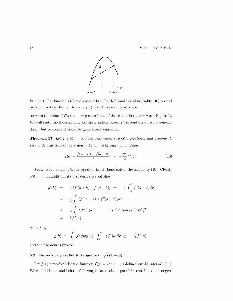
Consider a function f(x), let h > 0, and consider the secant to f(x) at the points x =

a±h, as shown in Figure 1. The next theorem gives a lower bound on the difference ∆


x

∆

a − h a a + h

Figure 1: The function f(x) and a secant line. The left-hand side of inequality (10) is equal

to ∆, the vertical distance between f(x) and the secant line at x = a.

between the value of f(a) and the y-coordinate of the secant line at x = a (see Figure 1).

We will state the theorem only for the situation where f ’s second derivative is concave

down, but of course it could be generalized somewhat.

Theorem 17. Let f : R → R have continuous second derivatives, and assume its

second derivative is concave down. Let a, h ∈ R with h > 0. Then

f(a) − f(a + h) + f(a − h)2

> − h2

2f ′′(a). (10)

Proof. Fix a and let g(h) be equal to the left-hand side of the inequality (10). Clearly

g(0) = 0. In addition, its first derivative satisfies

g′(h) = − 12 (f ′(a + h) − f ′(a − h)) = − 1

2

∫ h

−h

f ′′(a + x)dx

= − 12

∫ h

0

(f ′′(a + x) + f ′′(a − x))dx

≥ − 12

∫ h

0

2f ′′(a)dx by the concavity of f ′′

= −hf ′′(a).

Therefore,

g(h) =∫ h

0

g′(y)dy ≥∫ h

0

−yf ′′(a)dy ≥ − h2

2 f ′′(a),

and the theorem is proved.

5.2. On secants parallel to tangents of√

p(1 − p)

Let f(p) henceforth be the function f(p) =√

p(1 − p) defined on the interval [0, 1].

We would like to establish the following theorem about parallel secant lines and tangent


0 1x

a a+h2a−h1

Figure 2: Illustration of Theorem 18.

lines to f . For future reference, we compute the first and second derivatives of f :

f ′(x) =1 − 2x

2√

x(1 − x)and f ′′(x) =

−14(x(1 − x))3/2

.

It is easy to verify that the second derivative is concave down.

Theorem 18. Suppose 0 ≤ a − h1 < a < a + h2 ≤ 1. Further suppose that

f ′(a) =f(a + h2) − f(a − h1)

h2 + h1. (11)

Then h1 ≤ 3h2 and h2 ≤ 3h1.

The situation of Theorem 18 is sketched in Figure 2. Equation (11) says that the

slope of the secant line containing the points (a−h1, f(a−h1)) and (a+h2, f(a+h2)) is

equal to the slope of the line tangent to f at f(a). There are several simple observations

to make. First, by the concavity of f , if the values of a and h2 are fixed (respectively, the

values of a and h1 are fixed), then there is at most one value for h1 ∈ [0, 1] (respectively,

h2 ∈ [0, 1]) such that equation (11) holds. Second, since f ′ is a strictly decreasing

function, the value of a is uniquely determined by the values of a − h1 and a + h2.

Third, the theorem is easily seen to be true for a = 1/2, since in that case, h1 = h2.

Fourth, since f is symmetric around a = 1/2 with f(x) = f(1− x), it suffices to prove

that h2 ≤ 3h1 as h1 ≤ 3h2 will then follow by symmetry.

Before starting the proof of Theorem 18, it is useful to note that the graph of the

function f(x) =√

x(1 − x) forms the upper half of the circle of radius 1/2 with center

at the point (12 , 0). To prove this, just note that

√x(1 − x) =

√(1/2)2 − (x − 1/2)2.

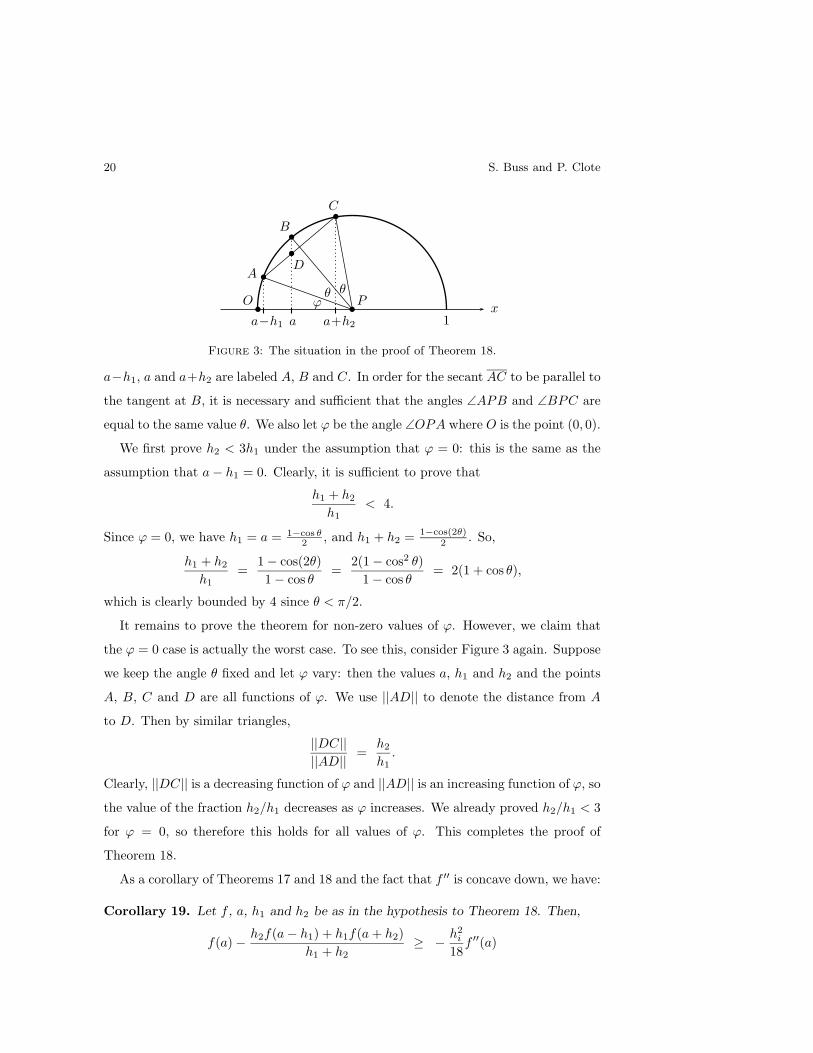
Therefore, the situation of Theorem 18 is as illustrated in Figure 3. In the figure, the

center of the semicircle is labeled P and the three points on the graph of f(x) at x =


O P

1x

A

B

D

C

ϕθ θ

a a+h2a−h1

Figure 3: The situation in the proof of Theorem 18.

a−h1, a and a+h2 are labeled A, B and C. In order for the secant AC to be parallel to

the tangent at B, it is necessary and sufficient that the angles ∠APB and ∠BPC are

equal to the same value θ. We also let ϕ be the angle ∠OPA where O is the point (0, 0).

We first prove h2 < 3h1 under the assumption that ϕ = 0: this is the same as the

assumption that a − h1 = 0. Clearly, it is sufficient to prove that

h1 + h2

h1< 4.

Since ϕ = 0, we have h1 = a = 1−cos θ2 , and h1 + h2 = 1−cos(2θ)

2 . So,

h1 + h2

h1=

1 − cos(2θ)1 − cos θ

=2(1 − cos2 θ)

1 − cos θ= 2(1 + cos θ),

which is clearly bounded by 4 since θ < π/2.

It remains to prove the theorem for non-zero values of ϕ. However, we claim that

the ϕ = 0 case is actually the worst case. To see this, consider Figure 3 again. Suppose

we keep the angle θ fixed and let ϕ vary: then the values a, h1 and h2 and the points

A, B, C and D are all functions of ϕ. We use ||AD|| to denote the distance from A

to D. Then by similar triangles,

||DC||||AD|| =

h2

h1.

Clearly, ||DC|| is a decreasing function of ϕ and ||AD|| is an increasing function of ϕ, so

the value of the fraction h2/h1 decreases as ϕ increases. We already proved h2/h1 < 3

for ϕ = 0, so therefore this holds for all values of ϕ. This completes the proof of

Theorem 18.

As a corollary of Theorems 17 and 18 and the fact that f ′′ is concave down, we have:

Corollary 19. Let f , a, h1 and h2 be as in the hypothesis to Theorem 18. Then,

f(a) − h2f(a − h1) + h1f(a + h2)h1 + h2

≥ − h2i

18f ′′(a)


for both i = 1, 2.

Proof. Let hmin = min{h1, h2}. Consider the two secant lines S1 and S2 where S1

is secant to the graph of f at x = a − h1 and x = a + h2, and S2 is the secant line at

x = a − hmin and x = a + hmin. The value (h2f(a − h1) + h1f(a + h2))/(h1 + h2) is

the y-coordinate of the secant line S1 at x = a. By the fact that f is concave down,

the secant line S2 is above the line S1 for a− hmin < x < a + hmin, and, in particular,

S2 is above S1 at x = a. By Theorem 17,

f(a) − h2f(a − h1) + h1f(a + h2)h1 + h2

≥ − h2min

2f ′′(a).

And by Theorem 18, for i = 1, 2, we have hi ≤ 3hmin, and this proves the corollary.

5.3. On secants parallel to tangents of the entropy function

The entropy function H(p) = −p ln(p) − (1 − p) ln(1 − p) is defined on the interval

[0, 1]. Its first and second derivatives are

H ′(p) = − ln(p) + ln(1 − p) = ln((1 − p)/p) = ln( 1p − 1)

H ′′(p) =−1

1 − p− 1

p=

−1(1 − p)p

.

It is easy to check that H ′(p) is strictly decreasing and is concave up for p ≤ 1/2 and

concave down for p ≥ 1/2. Also, H ′′(p) is concave down.

The next theorem states that H(p) satisfies the same kind of property that Theo-

rem 18 established for√

p(1 − p).

Theorem 20. Suppose 0 ≤ a − h1 < a < a + h2 ≤ 1. Further suppose that

H ′(a) =H(a + h2) − H(a − h1)

h2 + h1. (12)

Then h1 ≤ (e − 1)h2 and h2 ≤ (e − 1)h1, where e is the base of the natural logarithm.

We shall prove a weaker form of this theorem, namely, that there is a constant c

such that h1 ≤ ch2 and h2 ≤ ch1, and then appeal to experimental results obtained by

graphing functions in Mathematica to conclude that c = (e − 1) works.

The entropy function H(p) is qualitatively similar to the function f(p) =√

p(1 − p)

in that it is concave down, is zero at p = 0 and p = 1, and attains its maximum at

p = 1/2. So, Figure 2 can also serve as a qualitative illustration of Theorem 20. We


introduce new variables, and let r = a − h1 and s = a + h2. Suppose the values r, a, s

satisfy equation (12), that is, they satisfy

H ′(a) =H(s) − H(r)

s − r. (13)

Then, the values r, a, s are dependent in that any two of them determine the third.

To prove the theorem, we must give upper and lower bounds on the ratio h2/h1 =

(s − a)/(a − r). The values of r, s come from the set 0 ≤ r < s ≤ 1. The problem is

that this set is not compact by virtue of having an open boundary along the line r = s.

Even worse, the ratio is essentially discontinuous at r = s = 0 and at r = s = 1. For

our proof, we will examine the values of the ratio along the line r = s and at r = 0

(the case of s = 1 is symmetric), and argue by compactness of the remaining values of

r, s that the ratio attains a finite maximum value and a positive minimum value.

We assume w.l.o.g. that a < 1/2. When also s < 1/2, then we have h1 < h2 by the

fact that H ′(p) is concave up for p ≤ 1/2 and the fact that H ′(a) is the average slope

of H(p) for p ∈ [r, s]. Thus, for s < 1/2, it suffices to prove that h1/(h1 + h2) ≥ 1/e

and thereby obtain h2 ≤ (e − 1)h1.

We start by proving the theorem in the case that r = 0. In this case,

H(s) − H(0)s − 0

=H(s)

s=

−s ln(s) − (1 − s) ln(1 − s)s

= ln(s−1(1 − s)−(1−s)/s).

To find the value of a such that H ′(a) equals this last value, we need to solve

1a− 1 = s−1(1 − s)−(1−s)/s.

We are really interested in the value of a/s, since with r = 0, we have a = h1 and

s = h1 + h2, and we need to establish a/s ≥ 1/e. Solving for a/s gives

a

s=

(1 − s)(1−s)/s

s(1 − s)(1−s)/s + 1. (14)

It is easy to check that lims→0+(1−s)1/s = 1/e. Therefore, as s → 0+ the quantity (14)

approaches the limit 1/e.

Now consider the case r = 0 and 0 < s ≤ 1 (so a1 ≤ 1/2). Let R(s) = a/s =

Y/(sY + 1), where Y (s) = (1 − s)(1−s)/s. The first derivative of R is

R′ =Y ′ − Y 2

(sY + 1)2(15)


with

Y ′ = Y

(− 1

s2ln(1 − s) − 1

s

).

Note the numerator of (15) is equal to

Y ·[− 1

s2ln(1 − s) − 1

s− (1 − s)(1−s)/s

]. (16)

The power series expansion for ln(1− s) shows that ln(1− s) < −s− s2 for 0 < s < 1.

Thus, (16) is positive and hence R(s) is increasing and 1/e < R(s) ≤ 1 for 0 < s ≤ 1.

We have proved the r = 0 case of the theorem (and by symmetry, the s = 1 case).

Now we consider the case where r ≈ s. First, if a = 1/2, then of course, s− a = a− r,

so h1 = h2 and the theorem is satisfied. More generally, compactness and continuity

considerations imply that there is a δ > 0 such that if |a − 1/2| < δ, then 1/(e − 1) <

(s−a)/(a− r) < e−1. (If δ = 1/2 works, we are done, but for now we just know there

is some such δ > 0.) Now, fix a value of a < 1/2 − δ. We consider values of r, s that

correspond to this value for a. Again, h2 = s − a and h1 = a − r. We are thinking of

h1 and h2 increasing in such way that a stays fixed.

We claim that as h1 and h2 increase, the ratio h2/h1 is increasing, at least for h2

and h1 not too large. In order to prove this, it is equivalent to prove that

dh2/dh1

h2/h1> 1.

With a fixed, taking the first derivative of equation (12) gives

0 = − dh1 + dh2

(h1 + h2)2(H(a + h2) − H(a − h1)) +

H ′(a + h2)dh2 + H ′(a − h1)dh1

h1 + h2.

So, using (12) again and multiplying by h1 + h2,

0 = − (dh1 + dh2)H ′(a) + H ′(a + h2)dh2 + H ′(a − h1)dh1.

Algebraic manipulation transforms this to

dh2/dh1

h2/h1=

h1(H ′(a − h1) − H ′(a))h2(H ′(a) − H ′(a + h2))

. (17)

H ′ is concave up and decreasing on [0, 1/2], thus for a − h1 ≥ 0 and a + h2 < 1/2,

h1(H ′(a − h1) − H ′(a)) > 2∫ a

a−h1

(H ′(x) − H ′(a))dx (18)

h2(H ′(a) − H ′(a + h2)) < 2∫ a+h2

a

(H ′(a) − H ′(x))dx. (19)


By∫ a

a−h1H ′(x)dx = H(a) − H(a − h1) and

∫ a+h2

aH ′(x)dx = H(a + h2) − H(a) and

using equation (12), the right-hand sides of (18) and (19) are equal. Therefore, (17) is

greater than 1. This shows that the ratio h1/h2 is decreasing as long as a + h2 ≤ 1/2

and a − h1 ≥ 0. If the Markov chain reaches a − h1 = 0 with a + h2 ≤ 1/2, then since

we already have proved that h1/h2 > 1/e at a−h1 = 0 it follows that h1/h2 > 1/e for

all values of h1 and h2 for this a.

On the other hand, if the Markov chain stops with a+h2 = 1/2 and a−h1 > 0, it is

sufficient to prove the following fact: For all r, a, s with r ≤ s−δ, we have h1/h2 > 1/e.

Now the set of points r, s with 0 ≤ r ≤ s − δ and s ≤ 1 is compact, and the ratio

h1/h2 is a continuous positive function of r, s. Thus it attains a minimum on this set.

By graphing the function with Mathematica it is seen that h1/h2 is bounded below

by 1/e by a fair margin. Thus we have proved the theorem. (If the reader dislikes

the use of Mathematica here, then she can take this as a proof that there exists some

constant c > 0, rather than as a proof that c = e − 1 works.)

Corollary 21. Let H, a, h1 and h2 be as in the hypothesis to Theorem 20. Then,

H(a) − h2H(a − h1) + h1H(a + h2)h1 + h2

≥ − h2i

2(e − 1)2H ′′(a)

for both i = 1, 2.

The proof of this corollary is identical to the proof of Corollary 19.

6. Proofs of the main theorems

This section presents the proofs of Lemmas 15 and 16, thus completing the proofs

of the main theorems.

6.1. The weak variation condition lemma

We present the proof of Lemma 16. Let f(x) =√

x(1 − x). Dividing equation (9)

by n, we need to prove that, for some α > 0,

f( in ) ≥ α

n +∑n

j=0mi,jf( j

n ), for all 0 < i < n. (20)

Fix i and assume w.l.o.g. that i ≤ n/2; a symmetric argument will work for i ≥ n/2.

It will help to work with vectors in R2, and we define Pj to equal the following point


(or vector) in R2:

Pj =(j, f( j

n )).

Consider the summation

P =∑n

j=0mi,jPj .

(P depends on i, but we suppress any mention of i in the notation.) We want to

establish an upper bound on the second coordinate of P. First, however, consider the

first component of P. The mean condition implies that∑n

j=0 jmi,j ≤ i since i ≤ n/2

(except that if this condition fails for i = n/2, then i = n/2 has to be handled in the

symmetric argument for the case i ≥ n/2). Therefore, P’s first coordinate is ≤ i.

To bound the second coordinate, let J be the set of values j such that |j−i| > δσ′i,n,

where δ is the value from the weak variation condition. Then,

P =∑

j 6∈J mi,jPj +∑

j∈J mi,jPj .

Let a = i/n, and let T be the line tangent to the graph of f(x) at x = a. Set h2 =

δσ′i,n/n and then choose h1 so that the secant line S which is secant to f at x = a−h1

and x = a + h2 is parallel to T . That is to say, we are in the situation of Theorem 18.

Thus, since a ≤ 1/2, we have h1 < h2 ≤ 3h1.

As f(x) is concave down, geometric considerations imply that each point Pj is on or

below the tangent line T . Also, for every j ∈ J , either j/n < a − h1 or j/n > a + h2.

Therefore, again since f is concave down, for every j ∈ J , the point Pj is on or below

the secant line S. By the weak variation condition,

∑j∈J

mi,j ≥ ε,

so in particular, the total weight of the points Pj which lie below the secant line S is

≥ ε. Define R to be the line parallel to T and S, lying between those lines, so that the

distance from T to R is equal to ε times the distance from T to S. Since all the points

Pj are on or below T , and the sum of the coefficients of Pj below the line S is ≥ ε, the

point P lies on or below the line R.

Let π2(P) denote the y-component of P, i.e., the value of the summation in (20).

Since the slope of R is non-negative and the first coordinate of P is ≤ i, the value


f( in )−π2(P) is greater than or equal to ε times the vertical distance between f(x) and

the secant line S at x = a = i/n. Thus, by Corollary 19,

f( in ) − π2(P) ≥ −ε

(h2)2

18f ′′(a) = − ε

(δσ′i,n/n)2

18f ′′(a)

= −εδ2i3/2(n − i)3/2

18n4· −1

4( i(n−i)n2 )3/2

=εδ2

72n−1.

To establish (20) and finish the proof of Lemma 16, choose α = εδ2/72.

6.2. The variation condition lemma

The proof of Lemma 15 is similar to the proof of Lemma 16, but uses H(p) in place

of f(p). We indicate only the changes in the proof. This includes defining J to be the

set of values j such that |j − i| > δσi,n, and letting h2 = δσi,n/n. At the end of the

proof, the calculations change. Using Corollary 21, we have

H( in ) − π2(P) ≥ −ε

(h2)2

2(e − 1)2H ′′(a) = − ε

(δσi,n/n)2

2(e − 1)2H ′′(a)

= −εδ2i(n − i)

2(e − 1)2n3· −1(1 − i

n ) in

=εδ2

2(e − 1)2n−1.

To finish the proof of Lemma 15, set α = eδ2/(2(e − 1)2).

Acknowledgements. We thank W.J. Ewens, I. Abramson, and an anonymous

referee for helpful comments.

Appendix A. Proofs of variation conditions

We prove the variation condition holds for both the binomial and the hypergeometric

distributions. Fix a Markov chain with transition matrix M on states 0, . . . , n, and fix

i with 1 ≤ i ≤ n − 1. Define

ak = mi,i+k,

for all k such that 0 ≤ i + k ≤ n. We say that the unimodal property holds provided

that ak ≥ ak+1 for all k ≥ 0 and that ak ≥ ak−1 for all k ≤ 0.

Lemma 22. Suppose M is a transition matrix satisfying the unimodal property. For

each i, let k0 = dσi,ne (we suppress in the notation the dependence of k0 on i). Suppose


that there is a constant α > 0 such that, for all i,

ak0 > α · a0 and a−k0 > α · a0.

Then the variation condition holds with any δ < 12 and ε = α/(1 + α).

Proof. Fix i, 1 ≤ i ≤ n − 1. We need to show that∑k:|k|>δσi,n

ak∑k ak

>α

1 + α. (21)

First consider ak’s for non-negative values of k. By the unimodal property,

∑0≤k≤δσi,n

ak ≤∑

0≤k≤δσi,n

a0 ≤ k0

2a0.

Similarly, ∑k>δσi,n

ak ≥∑

δσi,n<k≤k0

ak0 ≥ k0

2ak0 > α

k0

2a0.

Therefore, ∑k>δσi,n

ak∑k≥0 ak

>α(k0/2)a0

(k0/2)a0 + α(k0/2)a0=

α

1 + α.

A similar argument shows that∑(−k)>δσi,n

ak∑(−k)≥0 ak

>α

1 + α.

The previous two equations imply the desired condition (21).

Proof. (of Theorem 3). Let qi,j be the hypergeometric probabilities given in (2).

Fix n. Also fix some i ∈ {1, . . . n − 1}. Let σ =√

i(n − i)/n, and let k0 = dσe. Let

ai,k = qi,i+k. By Lemma 22, it will suffice to show that ak0/a0 > α and a−k0/a0 > α,

for some constant α. By the symmetry of the hypergeometric probabilities, ak = a−k,

so we may assume w.l.o.g. that i ≤ n/2, and prove only ak0/a0 > α. An easy calculation

shows thatak

ak−1=

(i − k + 1)(n − i − k + 1)(i + k)(n − i + k)

. (22)

With k = 1, 2, this is

a1

a0=

i(n − i)(i + 1)(n − i + 1)

anda2

a1=

(i − 1)(n − i − 1)(i + 2)(n − i + 2)

.


For k ≤ k0, we have

ak

a0=

a1

a0

a2

a1· · · ak

ak−1

=i(i − 1)(i − 2) · · · (i − k + 1) · (n − i)(n − i − 1) · · · (n − i − k + 1)

(i + 1)(i + 2)(i + 3) · · · (i + k) · (n − i + 1)(n − i + 2) · · · (n − i + k)

=i

i + k· i − 1i + k − 1

· · · i − k + 1i + 1

· n − i

n − i + k· n − i − 1n − i + k − 1

· · · n − i − k + 1n − i + 1

=k−1∏j=0

i − j

i − j + k·

k−1∏j=0

n − i − j

n − i − j + k

>

(i + 1 − k

i + 1

)k (n − i − k + 1

n − i + 1

)k

=(

1 − k

i + 1

)k (1 − k

n − i + 1

)k

> exp(− βk2

i + 1

)· exp

(− βk2

n − i + 1

)where β = 2 ln 2

> exp(−βk2

i

)· exp

(− βk2

n − i

)= exp

(− βnk2

i(n − i)

).

The inequality introducing the β factor deserves justification. Note k/(i + 1) ≤k0/(i + 1) ≤ 1/2 for all i and n. Likewise, k/(n − i + 1) ≤ 1/2. The inequality follows

from the the fact that (1 − c)c < e−βc for 0 < c ≤ 1/2.

Consider the case of k = k0. Note k0 ≤ i since k0 =⌈√

i(n − i)/n⌉≤

⌈√i⌉. Also,

nk20/(i(n − i)) ≤ 1, since k0 ≥ σ =

√i(n − i)/n. Thus,

ak0

a0> e−β =

14.

This completes the proof of the theorem.

Proof. (of Theorem 2). Consider the binomial probabilities pi,j as defined by (1).

Fixing i, and letting ak = pi,i+k, we have

ak

ak−1=

(n − i − k + 1)i(i + k)(n − i)

anda−k

a−(k−1)=

(i − k + 1)(n − i)(n − i + k)i

.

Both the quantities are clearly less than the corresponding ratio (22) obtained for the

hypergeometric probabilities. Hence, by the previous proof,

ak0

a0>

14

anda−k0

a0>

14,

and, by Lemma 22, the proof is completed.


References

[1] Avise, J., Neigel, J. and Arnold, J. (1984). Demographic influences on mito-

chondrial DNA lineage survivorship in animal populations. Journal of Molecular

Evolution 20, 99–105.

[2] Cann, R., Stoneking, M. and Wilson, A. (1987). Mitochondrial DNA and

human evolution. Nature 325, 31–36. 1 Jan 1987.

[3] Cannings, C. (1974). The latent roots of certain Markov chains arising in genetics

I: Haploid models. Advances in Applied Probability 6, 260–290.

[4] Donnelly, P. (1991). Weak convergence to a Markov chain with an entrance

boundary: Ancestral processes in population genetics. Annal of Probability 19,

1102–1117.

[5] Ewens, W. (1963). The mean time for absorption in a process of genetic type.

J. Austral. Math. Soc. 3, 375–383.

[6] Ewens, W. (1964). The pseudo-transient distribution and its uses in genetics. J.

Appl. Prob. 1, 141–156.

[7] Ewens, W. (1979). Mathematical Population Genetics. Springer-Verlag, Berlin.

[8] Feller, W. (1951). Diffusion processes in genetics. In Proc. 2nd Berkeley Sym-

posium on Mathematical Statistics and Probability. ed. J. Neyman. University of

California Press, Berkeley. pp. 227–246.

[9] Feller, W. (1968). An Introduction to Probability Theory and its Applications.

J. Wiley and Sons, Inc., New York. Volume 1, Third Edition.

[10] Fisher, R. (1930). The Genetical Theory of Natural Selection. Clarendon Press,

Oxford.

[11] Karlin, S. and McGregor, J. (1966). The number of mutant forms maintained

in a population. In Fifth Berkeley Symposium of Mathematical Statistics and

Probability. vol. 4. University of California Press, Berkeley pp. 403–414.


[12] Kimura, M. (1955). Solution of a process of random genetic drift with a contin-

uous model. Proc. Natl. Acad. Sci. USA 41, 144–150.

[13] Kimura, M. (1962). On the problem of fixation of mutant genes in a population.

Genetics 47, 713–719.

[14] Kimura, M. (1964). Diffusion models in population genetics. J. Appl. Prob. 1,

177–232.

[15] Kingman, J. F. C. (1982). The coalescent. Stochastic Processes and their Appli-

cations 13, 235–248.

[16] Kingman, J. F. C. (1982). Exchangeability and the evolution of large of

populations. In Exchangeability in Provability and Statistics. ed. G. Koch and

F. Spizzichino. North Holland, Amsterdam pp. 97–112.

[17] Kingman, J. F. C. (1982). On the genealogy of large populations. J. Appl. Prob.

19A, 27–43. Essays in Statistical Science, Papers in honor of P.A.P. Moran.

[18] Mohle, M. (1998). Robustness results for the coalescent. J. Appl. Prob. 35,

438–447.

[19] Mohle, M. (1999). The concept of duality and applications to Markov processes

arising in neutral population genetics models. Bernoulli 5, 761–777.

[20] Mohle, M. (2004). The time back to the most recent common ancestor in ex-

changeable population models. Advances in Applied Probability 36, 78–97.

[21] Schensted, I. (1958). Appendix model of subnuclear segregation in the macronu-

cleus of ciliates. American Naturalist 92 (864), 161–170.

[22] Takahata, N. and Crow, J. (1994). Population Genetics, Molecular Evolution,

and the Neutral Theory: Selected Papers of M. Kimura. University of Chicago

Press, Chicago and London.

[23] Tavare, S. (1995). Calibrating the clock: Using stochastic processes to measure

the rate of evolution. In Calculating the Secrets of Life: Applications of the Mathe-

matical Sciences in Molecular Biology. ed. E. Lander and M. Waterman. National

Academy Press, Washington, DC pp. 114–152.


[24] Tavare, S. (1997). Ancestral inference from DNA sequence data. In Case Studies

in Mathematical Modeling: Ecology, Physiology, and Cell Biology. ed. H. Othmer

et al. Prentice-Hall, Upper Saddle River, N.J. pp. 91–96.

[25] Watterson, G. (1962). Some theoretical aspects of diffusion theory in population

genetics. Ann. Math. Statist. 33, 93–957. Correction: 34,352.

[26] Watterson, G. (1996). Motoo Kimura’s use of diffusion theory in population

genetics. Theoretical population biology 49, 154–158.

[27] Wright, S. (1945). The differential equation of the distribution of gene frequen-

cies. Proc. Natl. Acad. Sci. USA 31, 382–389.

[28] Wright, S. (1949). Adaptation and selection. In Genetics, Paleontology and

Evolution. ed. G. Jepson, G. Simpson, and E. Mayr. Princeton University Press,

Princeton, N.J. pp. 365–389.

solving the fisher-wright and coalescence prob …sbuss/researchweb/markov/paper.pdf · applied...

Documents