annex 3: an explanation of oil peaking - gov.uk
TRANSCRIPT

An Explanation of Oil Peaking - December 2009
An Explanation of Oil Peaking
R.W. Bentley
Visiting Research Fellow, Department of Cybernetics, University of Reading, UK. [email protected] - 22 December 2009
Contents 1. Introduction 1 2. The Mechanism of the Conventional Oil Peak 2 3. The Example of the UK 8 4. Other Countries, & The World 19 5. The Global Production Peak of ‘All-Liquids’ 57 6. Some Forecasts that have ignored Peak, and Explanations 59 7. Conclusions 62 Annex: Some ‘Economic’ views of Oil Depletion 66 Notes & References 68 Acknowledgements 71 1: Introduction The resource-limited peak of conventional oil production is not an obvious phenomenon, and many analysts do not understand it. This report sets out to explain the concept, and to give reasons why it is poorly understood. It is perhaps natural to think that if a region contains a large amount of oil that can be extracted at relatively low cost, and only a fairly small proportion of this will be used over the period of a production forecast, then the forecast need not consider resource availability. This is usually expressed as “There is plenty of oil to meet the foreseeable demand”. Examples of this view, from the IEA, the British government, oil companies, and academic institutions are given below in Section 6. Early in a region’s oil development such a view can be correct. But once oil discovery is fairly mature this view is generally wrong. Section 2 sets out why this is the case. Section 3 takes the UK as a specific example, and Section 4 presents similar analysis for other regions, and for the world as a whole. Section 5 then explains why a production peak is probably also expected for ‘all-liquids’, although not in this case a resource-limited peak. Section 6, as already mentioned, lists some forecasts that have ignored peaking, and gives reasons for this. Section 7 presents conclusions.
1

An Explanation of Oil Peaking - December 2009
2: The Mechanism of the Conventional Oil Peak At the outset it is important to recognise that the world can potentially access very large quantities of oil. This includes not only conventional oil, but also heavy oils, oil from tar sands and oil shales, natural gas liquids, and the conversion of gas or coal to oil. The IEA recently estimated the long-term potentially recoverable resource base of all oils to be nearly 10 trillion barrels. In addition, oil can come from biofuels; and mankind can substitute away from oil - for example by gas or electrically-powered vehicles. Given that the world has used just over 1 trillion barrels of oil to-date, and the forecast amount required for the next 30 years is also around 1 trillion barrels, there would seem to be little risk of an imminent supply constraint. To understand why there is indeed a concern we need to look at the production of conventional oil. We define the latter as the fairly easily flowing oil that can be produced by primary or secondary extraction methods (including own-pressure, physical lift, water flood, and pressure maintenance from water or natural gas injection); as well as that already recovered, or scheduled to be recovered, by tertiary extraction (such as steam heating, nitrogen or CO2 injection, or miscible flood). On this definition over 85% of all oil produced to-day is conventional oil. The question that then lies at heart of the peaking argument is: How is the production of conventional oil in a region constrained over time? This turns out to be a rather complex question, so we approach the answer in steps. Let us start with a simplified view of oil production in a region, as given by Figure 1a.
0
10
20
30
40
50
1 3 5 7 9 11 13 15 17 19 21 23 25 27 29 31 33 35 37 39 41
Years
Ann
ual P
rodu
ctio
n(a
rbitr
ary
units
)
Figure 1a: A simplified model of why production in a region goes over peak.
2

An Explanation of Oil Peaking - December 2009
Here each triangle represents the production from a single field. As can be seen, it is assumed that production from each field starts in succeeding years; and that each field is smaller than the preceding one; in this case, 90% of the size. From these simple assumptions two perhaps surprising properties emerge: - Production reaches a peak when about one-third of the total oil indicated on the plot has been produced. - The peak is resource-limited, driven by the amount of oil in the large early fields. As the Figure indicates - but by all means create your own spreadsheet to verify - the smaller later fields, no matter how numerous or how much oil they contain in total, do not affect peak; they just fatten and extend the tail. Crucially - although the peak looks fairly obvious in this diagram, it is completely counter-intuitive when looked at with the forecasting tools of most analysts. How so? Here, if the first field starts production in year-1; then the region reaches peak in year-12. If one draws a line on the graph at year-10, what would most analysts see at that date? - That production has risen rapidly in the past, and is still trending upward (see Figure 1b). - There are large quantities of remaining reserves in the fields already in production. (Assume that fields are discovered 5 years before getting into production. Then the reserves at year-10 are as shown in Figure 1c, where field 1 still has nearly half its original reserves; fields 2 to 9 considerably more; field 10 is only just coming into production; and reserves have also been assessed for fields 11 to 15.) - These reserves are mostly low-cost. Much is in fields already in production, where the incremental cost of production is low; and reserves in the fields not yet in production are in a region where the geology is understood and some infrastructure already in place. - Discovery is continuing (the smaller later fields shown on Figure 1c have not been found by year-10). - Technology is moving on apace; so recovery factors in the existing fields are increasing.
3

An Explanation of Oil Peaking - December 2009
What to forecast at Year-10? (1) Production has been rising rapidly
0
10
20
30
40
50
1 3 5 7 9 11 13 15 17 19 21 23 25 27 29 31 33 35 37 39 41
Years
Ann
ual P
rodu
ctio
n(a
rbitr
ary
units
)Year-10
Figure 1b: The view at year-10 - The production trend.
0
10
20
30
40
50
1 3 5 7 9 11 13 15 17 19 21 23 25 27 29 31 33 35 37 39 41
Years
Ann
ual P
rodu
ctio
n(a
rbitr
ary
units
)
What to forecast at Year-10?(2) Reserves are large (World: 40 years' of reserves) (3) New fields are being discovered (e.g., Tupi)(4) Technology is increasing recovery factors (e.g., 4-D seismic)
Year-10
Produced ReservesYet-to-find
Figure 1c: The view at year-10 - Reserves, new fields, and technology.
4

An Explanation of Oil Peaking - December 2009
The above point is so important that it is worth re-iterating. If you are a forecaster and look only at: - past production, - reserves (or even the expected total recoverable resource), - the current rate of discoveries, - and the march of technology; and meet the oil required for your forecast out of the total oil available that seems reasonable on the above data, then you will get caught out by the peak. Many analysts, at the equivalent of ‘year-10’, have naively predicted production increases throughout their forecast period. Shortly we will look at the main factor that indicates if peak is expected. But first we ask how realistic is the above simple model - are we concluding too much from an over-simplification? The first thing to note is that the shape of the production curve in Figure 1a is a surprisingly good approximation of reality. Based on US experience of regions and individual States going over peak, this was the shape that Hubbert drew in his early paper predicting US peak; and which he later depicted in an interview on film. Many sizeable regions of the world are now past their conventional oil resource-limited peak - over 60 countries, and many on-shore and offshore regions within these countries - so there is plenty of evidence to show that the production profile in Figure 1a is indeed typical; see the examples later in this report. (This is true of course only for regions where production has not been significantly constrained by other factors; OPEC quotas being a case in point.) Although the production profile depicted in Figure 1a is realistic, we need to look in detail at the assumptions behind the model to elucidate the mechanism that drives peaking. First we examine the shape of production profile assumed for individual fields. It is important that they are roughly triangular? Real fields display a great variety of profiles, but - at least in more recent times, and for fields not excessively constrained by pipeline or FPSO capacity - a quick rise to full production, a fairly short plateau, and a long decline is typical. However, the model is fairly robust to the individual field profiles. M. Smith of Energyfiles Ltd., for example, has modelled the addition over time of fields with a fairly complex profile and finds a similar regional peak; while if one takes the extreme case where all fields have essentially constant-flow rectangular profiles, the regional peak is again clear, albeit sharper and later than in Figure 1a. The conclusion is that for all realistic field profiles, the regional peak from combining these fields occurs before or near a region’s ‘half-way’ production point. The second aspect of the model are the assumptions that fields come on-stream in regular succession, and that each field is 90% the size of the preceding one. The 90% ratio used
5

An Explanation of Oil Peaking - December 2009
here is based very roughly on that for UK North Sea fields, but it turns out that the model is remarkably insensitive to both field size distribution and rate they come on-stream, as long as the key feature is maintained that the smaller fields mostly come on-stream later. The latter is generally true - see the examples below - because the larger fields in a region are mostly easier to find, and because the economics of production helps ensure that large finds are put into production before smaller ones. Note that these assumptions reflect a complex intertwining of geology, knowledge, engineering and economics. The rate that fields are discovered in a region, and then brought on-stream, is affected by how fast geological knowledge of the region can be built up; the basic geology of how easy the big fields are to find compared to the smaller ones; and the economics that determines both the initial search effort, and the rate that new fields are brought into production. It is always possible, for example, for a surge of small fields to be brought on-stream rapidly – at least for a short while - as happened with UK production in 1999 when the oil price fell to $10/bbl. But analysts need to point to very special circumstances for the general features of the above model not to be valid. So what really drives the peak? It is the decline in discovery. If many new fields are being discovered that contain significant quantities of oil, then the added production of these fields can offset the decline from earlier fields. The resource-limited production peak only occurs once discovery in a region is well into decline. To know if the production peak is near it is therefore useful (though not essential) to see the discovery trend. Let us re-visit Figure 1a, and now add discovery. As before, it is assumed that discovery of each field takes place 5 years before its production starts, roughly in line with UK North Sea experience. This leads to Figure 2a, which shows both discovery and production data.
6

An Explanation of Oil Peaking - December 2009
0
20
40
60
80
100
-4 -1 2 5 8 11 14 17 20 23 26 29 32 35 38 41Years
Ann
ual D
isco
very
& P
rodu
ctio
n(a
rbitr
ary
units
)
Figure 2a: The simplified model of Figure 1a, showing both discovery by field, and each field’s
subsequent production, assuming that fields take 5 years from discovery to production. The
plot is to-scale, such that, for example, the volume of oil shown as discovered for field-1
(leftmost grey bar, 100 units) is the same as indicated for field-1 production (the lowermost
production triangle, which starts in year-1, reaches 9.09 units/yr. in year-2, and falls to zero by
year-23).
This is a very telling plot, and explains oil peaking. But for analysis purposes - to be able to predict peak, and also to be sure that no later peak will arrive - the data are best presented on a cumulative plot such as Figure 2b.
Estimating the Date of Peak: Cumulative data
0
100
200
300
400
500
600
700
800
900
1000
-4 -1 2 5 8 11 14 17 20 23 26 29 32 35 38 41
Years
Cum
ulat
ive
Dis
cove
ry &
Pro
duct
ion
(arb
itrar
y un
its)
Cumulative discovery
Cumulative production
URR ~ 1000 unitsPeak at 36% of URR;
at 44% of Cum. Discovery
Figure 2b: The same data as Figure 2a, but on a cumulative basis - discovery and production.
The resource-limited peak in production (at year-12) is shown by the square.
7

An Explanation of Oil Peaking - December 2009
As can be seen, by the time production of the first field starts in year-1, about 50% of the final discovery has occurred. By the time production peaks in year-12 the discovery curve has turned well towards asymptote. In the real world – see the examples below – the discovery asymptote is usually clear well before peak has occurred. Of course basins – and even more so larger regions – can be complex; and new plays can open up. In such cases the discovery trend for a region can display ‘multiple asymptotes’, and it takes geological knowledge to judge when overall discovery in the region is drawing to a close. This aspect is brought out in the example regions reported next. Summarising this section we can say: 1. The resource-limited conventional oil production peak in a region is caused by adding the output of successive fields, where the later fields are generally smaller than the earlier. This reflects the fact that the size distribution of fields in most areas is very skewed, with most of the oil being held in a relatively small number of large fields that tend to get found first. 2. The peak occurs once discovery has declined significantly; and indicates the point at which reduced output from the early fields is no longer compensated by increased production from the later. The typical shape of the regional production curve is driven by the profile of decline in individual fields, primarily from field pressure loss, drive fluid breakthrough, or both. In the case of this simple model, the peak of discovery is 16 years before the production peak. 3. The production peak is counter-intuitive. This is because it occurs when: - production has been trending steadily upward; - remaining reserves are large, and generally low-cost; - discovery is continuing; - technology is improving, and recovery factors are increasing. 4. If a region sees significant separate phases of discovery, such as on-shore followed by offshore, then production may also show a number of resource-limited peaks, each reflecting a different discovery phase. 3: Peaking of Conventional Oil - The Example of the UK Now we turn from a theoretical model to actual cases where the peak has occurred. Figure 3 shows the UK production of liquids (oil plus NGLs) from 1960 to 2000. In terms of peak, there was a peak in the mid 1980s, and perhaps a hint of one 1999. In terms of proved reserves, these were absolutely no help in identifying the peak; having remained
8

An Explanation of Oil Peaking - December 2009
unchanged at about 5 billion barrels (Gb) since the mid-1980s.
Figure 3: UK liquids (oil plus NGLs) production, 1960 – 2000.
Source: BP Statistical Review.
es Figure 4.
‘2P’) oil discovery (bars), and production (line).
Source: Energyfiles Ltd.
So to see what was happening one needs to look at the history of discovery, using the ‘proved plus probable’ (‘2P’) discovery data, rather than the much lower volumreported by the proved (‘1P’) reserves. The ‘2P’ discovery data are shown in
Figure 4: UK proved plus probable (
9
An Explanation of Oil Peaking - December 2009
As can be seen, discovery in the UK mirrors that given in the simple model of Section 2, with the bulk of UK discovery (by volume) taking place before offshore production started. Although discovery here is not broken out by field, the pattern was that once a small initial field had been discovered in 1969 nearly all the very large fields were discovered fairly rapidly thereafter. By comparing the volume discovered with the volume produced, the Figure indicates clearly that the 1984 peak was not resource-limited; but the 1999 peak was. In the UK’s case the trough between these two peaks was caused mainly by the safety work carried out on all fields following the Piper-Alpha disaster. (Lesser factors included the 2-year work-over on Brent due to high gas production, a fall in oil prices, hinted changes in petroleum revenue tax that may have delayed the start up of new
elds, and - as Laherrère notes - a secondary peak in discovery in the late 1980s.)
ak is caused by the larger fields mostly getting into production first is early borne out.
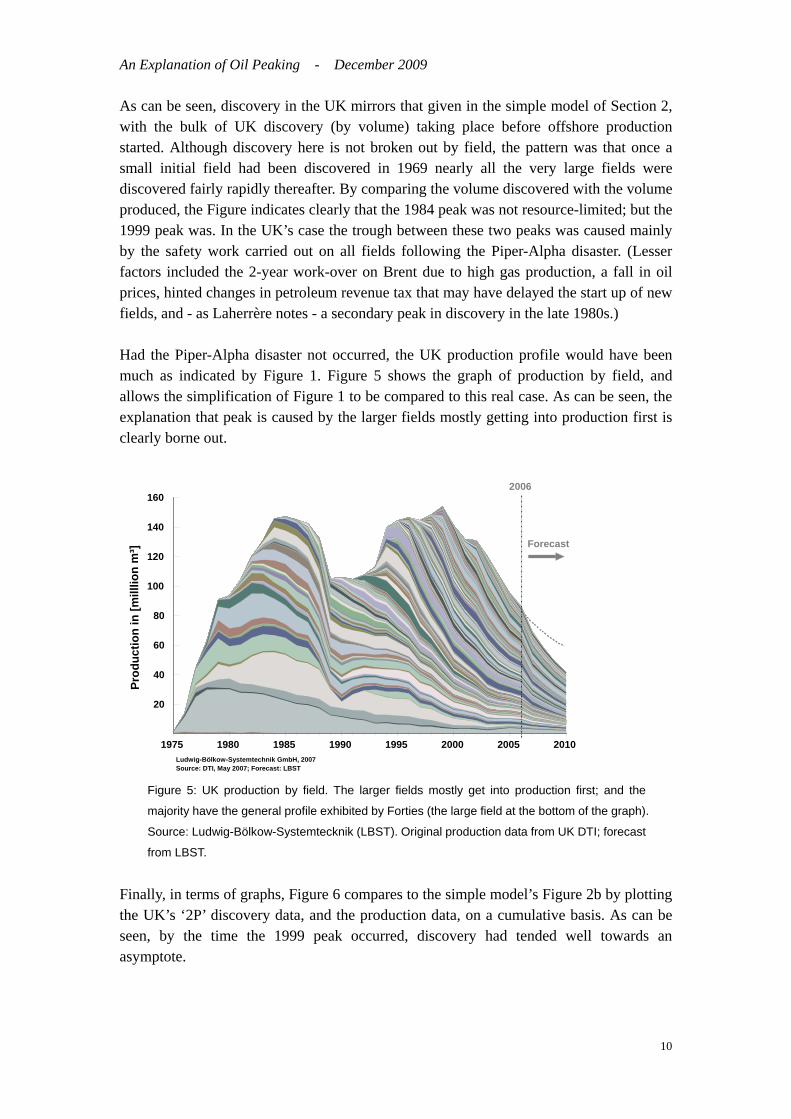
fi Had the Piper-Alpha disaster not occurred, the UK production profile would have been much as indicated by Figure 1. Figure 5 shows the graph of production by field, and allows the simplification of Figure 1 to be compared to this real case. As can be seen, the explanation that pecl
1975 1980 1985 1990 1995 2000 2005 2010
20
40
60
80
100
120
140
160
Prod
uctio
n in
[mill
lion
m³]
2006
Forecast
Ludwig-Bölkow-Systemtechnik GmbH, 2007Source: DTI, May 2007; Forecast: LBST
Figure 5: UK production by field. The larger fields mostly get into production first; and the
majority have the general profile exhibited by Forties (the large field at the bottom of the graph).
Source: Ludwig-Bölkow-Systemtecknik (LBST). Original production data from UK DTI; forecast
from LBST.
e the 1999 peak occurred, discovery had tended well towards an symptote.
Finally, in terms of graphs, Figure 6 compares to the simple model’s Figure 2b by plotting the UK’s ‘2P’ discovery data, and the production data, on a cumulative basis. As can be seen, by the tima
10

An Explanation of Oil Peaking - December 2009
Figure 6: UK ‘2P’ oil discovery and production, displayed on a cumulative basis. Source:
Energyfiles Ltd. Also shown are four estimates for the UK’s conventional oil ‘ultimate’. The
UK Department of Energy’s estimate (‘DOE’) is from 1974; the others are more recent. The
Campbell/Uppsala and USGS year-2000 estimates exclude NGLs (these add ~4.5 Gb); the
USGS also excludes UK West of Shetlands basins.
Now we come to an important point. We have indicated that the 1999 peak is resource-limited, and clearly this is the case based on the oil already discovered (see Figure 4). But how do we know this will remain true in future? Perhaps the UK has big new plays waiting in the wings that in time will yield much greater quantities of oil, enough to surpass the 1999 peak. As has been mentioned, the situation often occurs where historical discovery data (the ‘creaming curve’ vs. time) indicates an apparent asymptote, but where this increases as a new play enters the scene. So what was known to indicate that the UK’s 1999 peak was indeed resource-limited; unlike, therefore, the 1984 peak? Knowledge of peak cannot be based solely on discovery data, it must also include geological appraisal. The latter will always be a judgement, and can never be known with absolute certainty. But a great deal of geological knowledge now exists for much of the world’s likely oil plays. In the UK’s case there are still several significant future potential sources of oil. There may be quite large quantities of oil undiscovered in subtle stratigraphic traps; there is new potential in the deeper Atlantic; and there are certainly large amounts of oil in-place currently deemed unrecoverable. But geological and reservoir knowledge says it is virtually certain that none of this oil, if it exists, can be developed rapidly enough to push UK production back up past the 1999 peak. The subtle
11
An Explanation of Oil Peaking - December 2009
traps, if they hold significant amounts of oil, will need highly calibrated seismic to find, so will not be found rapidly; the deeper Atlantic will offer surprises but is not thought especially prospective due to poor source rock and traps; while the many routes to improved recovery in existing fields have already seen much trial and analysis. Overall, combining the UK’s 2P discovery data with geological knowledge indicates that the country’s conventional oil peak in 1999 was indeed resource-limited. Figure 6 brings out this point by including four estimates of the UK’s ultimately recoverable resource (‘ultimate’). The earliest is a UK government DoE ‘Brown Book’ estimate made back in 1974, and the more recent are from Campbell, the USGS, and Energyfiles. These ‘ultimates’ are in close agreement with each other, and with the asymptote of the ‘2P’ discovery creaming curve. (As already indicated, the reason that the UK Department of Energy estimate made in 1974 for the UK ‘ultimate’ could be so accurate - before UK offshore production had even started - was that by 1974 most of the big fields had already been discovered.) An important question, therefore, is why did the 1999 peak – and perhaps more so, the very steep subsequent decline in production – come as such a surprise to the UK government? It should not have done so. Using the 1974 estimate of ultimate; and plotting a simple ‘mid-point’ isosceles triangle based on the initial production trend certainly finds peak at around the right date; a fact reported at the time (and see below, Figures 7b and 7c). But ‘mid-point’ peaking got forgotten (and not just in the UK, as we shall see), and a deep myth developed based on the behaviour of proved reserves. Table 1: UK Data on Reserves A: PROVED RESERVES (‘1P’) Year Gb Year Gb 1975 16.0 1991 4.0
1976 16.8 1992 4.1
1977 19.0 1993 4.6
1978 16.0 1994 4.5
1979 15.4 1995 4.3
1980 14.8 1996 4.5
1981 14.8 1997 5.0
1982 13.9 1998 5.2
1983 13.2 1999 5.2
1984 13.6 2000 5.0
1985 13.0 2001 4.9
1986 5.3 2002 4.7
1987 5.2 2003 4.5
1988 4.3 2004 4.5
1989 3.8 2005 4.0
12
An Explanation of Oil Peaking - December 2009
1990 3.8 2006 3.6
2007 3.6
(Source: BP Statistical Review, various dates.)
B: PROVED PLUS PROBABLE RESERVES (‘2P’) Year Gb
USGS 1996 9.7
C/U 2005 9.3
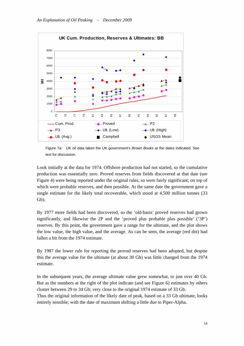
Note: C/U: Campbell / University of Uppsala As the table shows, the UK’s proved reserves from 1975 to 1985 were in the region of 15 Gb; but then dropped in 1986 to about 5 Gb, and stayed close to this figure until very recently. Of course, all that changed in 1986 was the basis of reporting. Proved plus probable (2P) reserves are currently about twice the proved value. (The full reason that the UK’s proved reserves have been so much below the 2P reserves still needs elucidating. It almost certainly reflects, in part, reserves reporting by oil companies under US Securities & Exchange Commission rules; but probably also the non-inclusion of reserves of discovered fields until sanctioned for development.) The long period of static values for UK proved reserves – staying at the equivalent of roughly 5 year’s supply - would not matter except that it fooled many analysts into thinking that something special was going on. Year after year oil was being produced, but the proved reserves were not falling. This replacement of the reserves was thus very widely ascribed, including within the oil industry, the UK government and the IEA, as being primarily due to improvements in technology; horizontal drilling and 4-D seismic being frequently cited. The real explanation was that as the proved reserves were produced, reserves in the probable category became classed as proved. But why did analysts not see this for what it was? The reason lies in the usual definition of proved reserves: “ ... those quantities that geological and engineering information indicate with reasonable certainty can be recovered in future under existing economic and operating conditions.” Most analysts then – and still today – treat proved reserves as a fairly accurate measure of the amount of oil likely to be available. The simple reality – that the quantities of oil likely to be recovered under existing economic and operating conditions are generally much larger than the proved reserves – was not recognised; and all too often is still not recognised today. Figure 7a, though a little complex to read, sets all this out plainly. It shows UK data on cumulative production, 1P and 2P reserves; and, importantly, shows the estimates made at the time of the total amount of oil likely to be recovered in UK waters (the ‘ultimate’). The data are taken from issues of the UK’s Brown Book for the years indicated.
13
An Explanation of Oil Peaking - December 2009
UK Cum. Production, Reserves & Ultimates: BB
0
1000
2000
3000
4000
5000
6000
7000
8000
73 75 77 79 81 83 85 87 89 91 93 95 97 99
Mt
Cum. Prod. Proved P2
P3 Ult. (Low) Ult. (High)
Ult. (Avg.) Campbell USGS Mean
Figure 7a: UK oil data taken the UK government’s Brown Books at the dates indicated. See
text for discussion.
Look initially at the data for 1974. Offshore production had not started, so the cumulative production was essentially zero. Proved reserves from fields discovered at that date (see Figure 4) were being reported under the original rules, so were fairly significant; on top of which were probable reserves, and then possible. At the same date the government gave a single estimate for the likely total recoverable, which stood at 4,500 million tonnes (33 Gb). By 1977 more fields had been discovered, so the ‘old-basis’ proved reserves had grown significantly, and likewise the 2P and the ‘proved plus probable plus possible’ (‘3P’) reserves. By this point, the government gave a range for the ultimate, and the plot shows the low value, the high value, and the average. As can be seen, the average (red dot) had fallen a bit from the 1974 estimate. By 1987 the lower rule for reporting the proved reserves had been adopted, but despite this the average value for the ultimate (at about 30 Gb) was little changed from the 1974 estimate. In the subsequent years, the average ultimate value grew somewhat, to just over 40 Gb. But as the numbers at the right of the plot indicate (and see Figure 6) estimates by others cluster between 29 to 34 Gb; very close to the original 1974 estimate of 33 Gb. Thus the original information of the likely date of peak, based on a 33 Gb ultimate, looks entirely sensible; with the date of maximum shifting a little due to Piper-Alpha.
14
An Explanation of Oil Peaking - December 2009
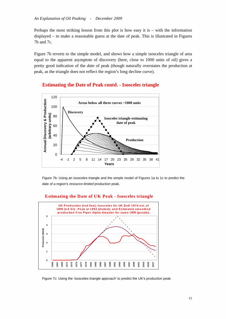
Perhaps the most striking lesson from this plot is how easy it is – with the information displayed – to make a reasonable guess at the date of peak. This is illustrated in Figures 7b and 7c. Figure 7b reverts to the simple model, and shows how a simple isosceles triangle of area equal to the apparent asymptote of discovery (here, close to 1000 units of oil) gives a pretty good indication of the date of peak (though naturally overstates the production at peak, as the triangle does not reflect the region’s long decline curve).
Estimating the Date of Peak contd. - Isosceles triangle
0
20
40
60
80
100
120
-4 -1 2 5 8 11 14 17 20 23 26 29 32 35 38 41Years
Ann
ual D
isco
very
& P
rodu
ctio
n(a
rbitr
ary
units
)
Areas below all three curves ~1000 units
Discovery
Isosceles triangle estimating date of peak
Production
Figure 7b: Using an isosceles triangle and the simple model of Figures 1a to 1c to predict the
date of a region’s resource-limited production peak.
Estimating the Date of UK Peak - Isosceles triangle
UK Production (red line); Isosceles for UK DoE 1974 est. ofURR (4.6 Gt) - Peak at 1992 (dotted); and Estim ated sm oothedproduction if no P iper Alpha d isaster for sam e URR (purple).
0
1
2
3
4
5
1965
1967
1969
1971
1973
1975
1977
1979
1981
1983
1985
1987
1989
1991
1993
1995
1997
1999
2001
2003
2005
2007
Prod
uctio
n (M
b/d )
Figure 7c: Using the ‘isosceles triangle approach’ to predict the UK’s production peak.
15

An Explanation of Oil Peaking - December 2009
Figure 7c shows the same procedure applied to estimate the date of the UK peak; and indicates both actual UK production, and an estimate of what it might have been had Piper-Alpha not occurred. An alternative, and more precise, analysis results if the original 1974 estimate for the UK’s ultimate of 4,600 Mt is used in combination with the standard ‘mid-point peaking’ rule. On this basis the UK’s resource-limited peak would be expected when the cumulative production reached 2,300 Mt. This was not in 1984 (when cumulative production had reached only about 700 Mt), but occurred at about 1998 or 1999. Given the general straightness of the cumulative production line, despite the trough from 1985 to 1995, this date could be (and was) predicted with reasonable precision from the first years of production. Piece of cake, really. It is reasonable to ask at this point: Where does economics come in? Economic factors are important, of course. A higher oil price encourages exploration, brings on economically marginal fields, permits more expensive recovery, and reduces demand. But in a country well past its discovery peak the effects are fairly small. More exploration just moves the country further along the long-declining discovery trend; the economically marginal fields are known, and are often small or difficult; and the more expensive recovery techniques can be identified and their impacts calculated. In general, though each country needs specific analysis, the ability of a higher oil price to significantly impact the geologically-based estimates of ultimate is usually fairly limited. However, having just said how easy is the topic, before we leave the UK data we will examine one of the uncertainties that do remain, that of evaluating the impact of reserves growth on a region’s date of peak. ‘Reserves growth’ as used here, and generally, means the increase over time in size of fields already discovered; i.e., for a region, it sums the growth of the original recoverable reserves (the ‘field ultimates’) of the individual fields. With the global volume-weighted average recovery factor of perhaps 35%, the scope for reserves growth in fields is large. Some modellers of future global production assume reserves growth as zero – effectively holding that the field ‘ultimates’ in the industry ‘2P’ datasets are pretty accurate; while other modellers assume extraordinarily high numbers for reserves growth. So it is important to gather what data we can. Firstly, of course we must rule out the simple apparent reserves growth that occurs as a field’s 1P data get updated over time to finally equal the true 2P (i.e. the most probable) value. Odell, for example, reported nine-fold growth for Western Canadian oil fields; while US fields exhibit typically a six-fold growth in size if on-shore, and about three-fold for offshore. These sort of percentage growths (i.e., up to 900%) are almost undoubtedly mainly due to moving from 1P to 2P numbers; with a physical explanation –
16

An Explanation of Oil Peaking - December 2009
at least for large fields – often being simply the ‘drilling-up’ of fields. Early in the life of a large field only a relatively small number of production wells are sunk, and under SEC rules only the oil judged in ‘direct communication’ with these wells can be classed as reserves. Over time an increasing number of production wells get drilled, increasing the area ‘in communication’, and thus raising reserves. Other large increases have occurred famously in large old heavy oil fields, where naturally reserves increases from improvements in recovery technology have been significant. The general rule on reserves growth, therefore, is to be very cautious of accepting data at face value. The data we seek, by contrast, are reasonably current data on ‘real’ (technology- or knowledge-driven) gains over time in field 2P values. Figure 8 shows such data for the UK.
0%
50%
100%
150%
200%
250%
300%
350%
1 5 9 13 17 21 25
Beryl Brent
Claymore Cormorant
Forties Fulmar
Magnus Ninian
Piper Schiehallion
MEAN
0%
50%
100%
150%
200%
250%
300%
350%
1 5 9 13 17 21 25
Montrose DunlinHeather ThistleAuk MurchisonTartan BeatriceMaureen BuchanHutton Northwest HuttonClyde Alwyn NorthBalmoral EiderTern ArbroathMiller Rob RoyOsprey TiffanyScott BruceSaltire NelsonGryphon CaptainHarding MungoFoinaven CurlewMEAN
Figure 8: Reserves growth for UK oil fields; ‘2P’ data. Data from R. Miller of BP.
Upper graph: UK large fields, showing the change in industry data for ‘proved plus
probable’ (2P) reserves with time after first declaration. The Beryl field seems to be anomalous
between years 18 and 22, but the trend of the data is clear: after 25 years, reserves for large
17

An Explanation of Oil Peaking - December 2009
fields had grown by some 50% on average.
Lower graph: UK small fields. The data are probably statistically unreliable by 25 years, as
few small fields have yet operated so long. Interestingly there is no significant change in
industry data for declared 2P reserves for 9 years, but then a steady growth sets in, reaching
25% after 25 years altogether. This might suggest a very good initial estimate of field size, with
only statistical fluctuation of the mean. After some 10 years, further exploration effort (driven by
approaching exhaustion?) has discovered a suite of satellite fields, stacked reservoirs and
other deposits entirely excluded from the initial estimates. Miller noted that “It would be
interesting know whether the large fields (> 500 mmbbl recoverable) grew from the discovery
of new pools.”
As Figure 8 shows, field growth is very variable between fields, but averaged over time, the large fields grew by about 50%; and the smaller fields by about 25%. These are significant increases, and should not be ignored in the modelling. But these values are less than one-tenth the US and Canadian ‘1P reserves becoming 2P’ reserves growth values of 600% to 900% reported above. And even with 2P reserves, a caution is needed. Campbell, with long experience in industry of field discovery, and of watching how the size of fields is reported over time, identifies a ‘U-shaped reporting curve’. This starts with an original ‘geological’ value, kept internal to the company, which is based on an estimate of oil in-place, and factored by an initial estimate of overall recovery factor. This is followed by the first published value, based on conservative engineering evaluation of the infrastructure likely to be initially committed. Then there is a slow reported growth in field size as subsequent investments are made in the field; with this growth often taking the field size back to close to the original ‘geological’ estimate. The evolution of the reported size of Prudhoe Bay, for example, has shown just this process, as confirmed by BP’s Gilbert. The main conclusions from this section on UK data are: - The simple model of Section 2 captures much of what happens in reality, at least for the UK. - The UK government forecast made in 1976, that the UK production peak would occur shortly before the year 2000, is easy to understand on the basis of the estimate for the UK’s ‘ultimate’ and the ‘mid-point peaking’ rule. - It was a pity that this comprehension of the mechanism of peaking got eroded over time, to be replaced by the widespread myth of very high levels of technology-driven reserves replacement – becoming the favoured explanation of why the UK’s 5 years’ of proved reserves had lasted for over 20 years without diminution. - Moderate levels of reserves growth do occur in 2P data however, at least as reported in industry datasets, and need to be accounted for. In the next section we look at how well the above understanding of peaking matches data for countries other than the UK.
18
An Explanation of Oil Peaking - December 2009
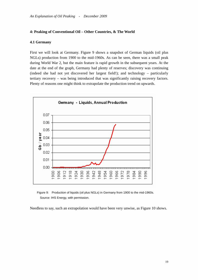
4: Peaking of Conventional Oil – Other Countries, & The World 4.1 Germany First we will look at Germany. Figure 9 shows a snapshot of German liquids (oil plus NGLs) production from 1900 to the mid-1960s. As can be seen, there was a small peak during World War 2, but the main feature is rapid growth in the subsequent years. At the date at the end of the graph, Germany had plenty of reserves; discovery was continuing (indeed she had not yet discovered her largest field!); and technology – particularly tertiary recovery – was being introduced that was significantly raising recovery factors. Plenty of reasons one might think to extrapolate the production trend on upwards.
Figure 9: Production of liquids (oil plus NGLs) in Germany from 1900 to the mid-1960s.
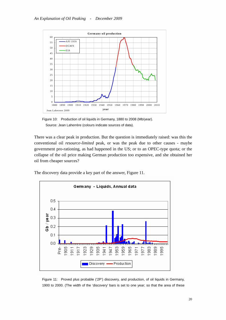
Source: IHS Energy, with permission. Needless to say, such an extrapolation would have been very unwise, as Figure 10 shows.
19
An Explanation of Oil Peaking - December 2009
G erm any o il production
0
5
10
15
20
25
30
35
40
45
50
55
60
1880 1890 1900 1910 1920 1930 1940 1950 1960 1970 1980 1990 2000 2010
year
A PI 1959
D GM N
E IA
Jean Laherrere 2009
Figure 10: Production of oil liquids in Germany, 1880 to 2008 (Mb/year).
Source: Jean Laherrère (colours indicate sources of data). There was a clear peak in production. But the question is immediately raised: was this the conventional oil resource-limited peak, or was the peak due to other causes - maybe government pro-rationing, as had happened in the US; or to an OPEC-type quota; or the collapse of the oil price making German production too expensive, and she obtained her oil from cheaper sources? The discovery data provide a key part of the answer, Figure 11.
Figure 11: Proved plus probable (‘2P’) discovery, and production, of oil liquids in Germany,
1900 to 2000. (The width of the ‘discovery’ bars is set to one year; so that the area of these
20
An Explanation of Oil Peaking - December 2009
bars and the corresponding final area under the production curve must be equal.) Source:
IHS Energy, with permission.
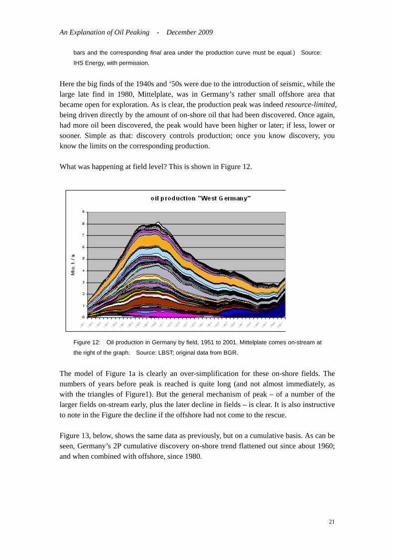
Here the big finds of the 1940s and ‘50s were due to the introduction of seismic, while the large late find in 1980, Mittelplate, was in Germany’s rather small offshore area that became open for exploration. As is clear, the production peak was indeed resource-limited, being driven directly by the amount of on-shore oil that had been discovered. Once again, had more oil been discovered, the peak would have been higher or later; if less, lower or sooner. Simple as that: discovery controls production; once you know discovery, you know the limits on the corresponding production. What was happening at field level? This is shown in Figure 12.
Figure 12: Oil production in Germany by field, 1951 to 2001. Mittelplate comes on-stream at
the right of the graph. Source: LBST; original data from BGR.
The model of Figure 1a is clearly an over-simplification for these on-shore fields. The numbers of years before peak is reached is quite long (and not almost immediately, as with the triangles of Figure1). But the general mechanism of peak – of a number of the larger fields on-stream early, plus the later decline in fields – is clear. It is also instructive to note in the Figure the decline if the offshore had not come to the rescue. Figure 13, below, shows the same data as previously, but on a cumulative basis. As can be seen, Germany’s 2P cumulative discovery on-shore trend flattened out since about 1960; and when combined with offshore, since 1980.
21

An Explanation of Oil Peaking - December 2009
Germany - Liquids, Cumulative data
0.0
0.5
1.0
1.5
2.0
2.5
3.0
1900 1920 1940 1960 1980 2000 2020
Gb
Discovery Prodn. Peak USGS: MeanCampbell/U BGR/Hiller Energyfiles
Prod. at peak 0.72 GbCampbell ult. 2.75 Gb Peak at 26 % of ult.
Figure 13: Cumulative oil liquids discovery (2P data), and production, Germany, 1900 to 2000.
Estimates for Germany’s conventional oil ‘ultimates’ are shown against the year 2025. (This
is notionally the year that applies to the USGS estimate, but in practice all four ‘ultimates’ refer
to much later dates.) Campbell/Uppsala exclude NGLs. USGS ultimate is the mean estimate
on a ‘non-grown’ basis. As USGS data sum only basins evaluated this total may exclude
Germany’s offshore. The date of the production peak is marked with a triangle.
Note that peak is given as occurring at 26% of the Campbell/Uppsala ultimate of 2.75Gb;
but as peak reflects the on-shore fields, this occurred at about 35% of the apparent on-shore
discovery asymptote, of about 2 Gb.
Sources: Discovery & Production: IHS Energy, with permission; ‘Ultimates’: see references. But, as in the UK, to know if the fall-off in discovery is misleading; i.e., to know whether or not there are still large quantities of oil waiting in the wings, one also needs geological knowledge. Estimates for the total amount of recoverable oil in Germany potentially accessible by a fairly distant future date have been made by various geological groups. These are ‘ultimates’, because they estimate the country’s ultimately recoverable reserves. They are best illustrated on a cumulative plot like Figure 13, which presents four such estimates: - BGR’s 1997 assessment of estimated ultimate recovery (‘EUR’): 2.3 Gb; - USGS’ year-2000 median assessment on a ‘non-grown’ basis, incl. NGLs: 2.14 Gb; - Campbell/University of Uppsala end-2004 model: 2.75 Gb; - Energyfiles end-2004 assessment: 2.6 Gb. Data sources are, respectively: BGR (1997), USGS (2000), Campbell/Uppsala, (2005), and Energyfiles (2005). Note that some of these data (for example, Campbell/Uppsala) exclude NGLs. Moreover, three of the groups recognise that future extraction technology and policies are unknown, so specifically caution that their figures should not be seen as definitive estimates of ‘true’
22

An Explanation of Oil Peaking - December 2009
ultimates (i.e. original endowments of recoverable conventional oil when extraction terminates). Instead the data refer to quantities of oil considered recoverable over reasonably long time spans. The USGS say they evaluate oil that will be available for discovery by 2025 (though there has been ambiguity reported around the meaning of this date). The Campbell/Uppsala model no longer lists ultimate, but ‘total regular oil production to 2075’ (‘regular’ oil here excludes polar, deepwater, very heavy oils and NGLs; in this model these latter oils are assessed separately, and summed in the production totals). Energyfiles quantifies oil that will have been produced by 2145. The BGR is the only organisation that uses the label ‘estimated ultimate recovery’, but probably would apply the same caveat as the others if asked. As the Figure shows, as was the case for the UK, the above ‘ultimates’ are in rough agreement with each other and with the apparent asymptote of the 2P discovery curve. The geologists are therefore pretty certain that no significant new quantities of oil will be found in Germany, where this reflects both geological knowledge and over a hundred years’ of discovery effort and technological progress. Like other regions of the world, Germany, despite having applied enhanced oil recovery (EOR) techniques since 1985, still has a considerable amount of oil judged currently unrecoverable in existing fields. However, barring some extraordinary new recovery technique, Germany is now close to the end of her conventional oil: at ~2.0 Gb Germany’s total production to-date has consumed about 80% of her recoverable original endowment. 4.2 Norway Next we look at comparable graphs for Norway. These are shown in Figures 14a to 14c. These indicate similar findings as for the UK and Germany.
Norway : Liquids - Annual Total Data
0
1
2
3
4
5
6
1965
1970
1975
1980
1985
1990
1995
2000
2005
Year
Gb/
Yea
r
DiscoveryProduction
Figure 14a. Norway - Annual 2P discovery and production. Industry data.
23

An Explanation of Oil Peaking - December 2009
Figure 14b. Norwegian oil production by field. Data: Uppsala University
Norway : Liquids - Cumulative Data
0
5
10
15
20
25
30
35
40
45
50
1955
1965
1975
1985
1995
2005
2015
2025
Year
Gb
DiscoveryProductionUSGS MeanCampbellPeak
Figure 14c. Cumulative plot of Norwegian oil 2P discovery and production; plus estimates of
URR (ultimately recoverable reserves). USGS mean URR (ex reserves growth) probably
reflects a lot of condensate. As can be seen, the Campbell URR plus the ‘mid-point rule’
correctly predicts the date of peak. Discovery & production: Industry data
24
An Explanation of Oil Peaking - December 2009
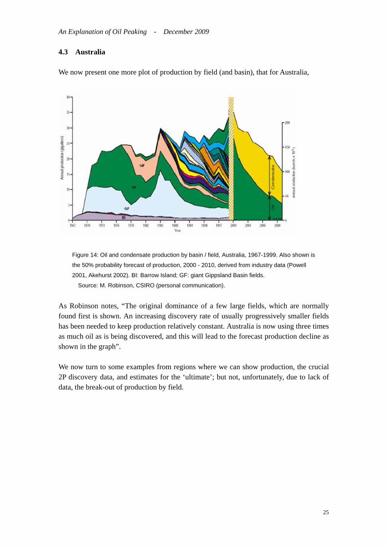
4.3 Australia We now present one more plot of production by field (and basin), that for Australia,
Figure 14: Oil and condensate production by basin / field, Australia, 1967-1999. Also shown is
the 50% probability forecast of production, 2000 - 2010, derived from industry data (Powell
2001, Akehurst 2002). BI: Barrow Island; GF: giant Gippsland Basin fields.
Source: M. Robinson, CSIRO (personal communication). As Robinson notes, “The original dominance of a few large fields, which are normally found first is shown. An increasing discovery rate of usually progressively smaller fields has been needed to keep production relatively constant. Australia is now using three times as much oil as is being discovered, and this will lead to the forecast production decline as shown in the graph”. We now turn to some examples from regions where we can show production, the crucial 2P discovery data, and estimates for the ‘ultimate’; but not, unfortunately, due to lack of data, the break-out of production by field.
25
An Explanation of Oil Peaking - December 2009
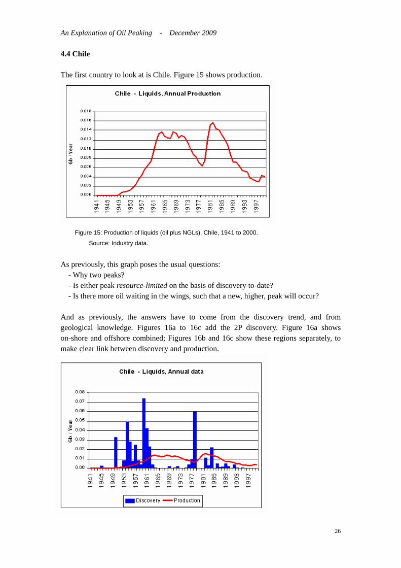
4.4 Chile The first country to look at is Chile. Figure 15 shows production.
Figure 15: Production of liquids (oil plus NGLs), Chile, 1941 to 2000.
Source: Industry data.
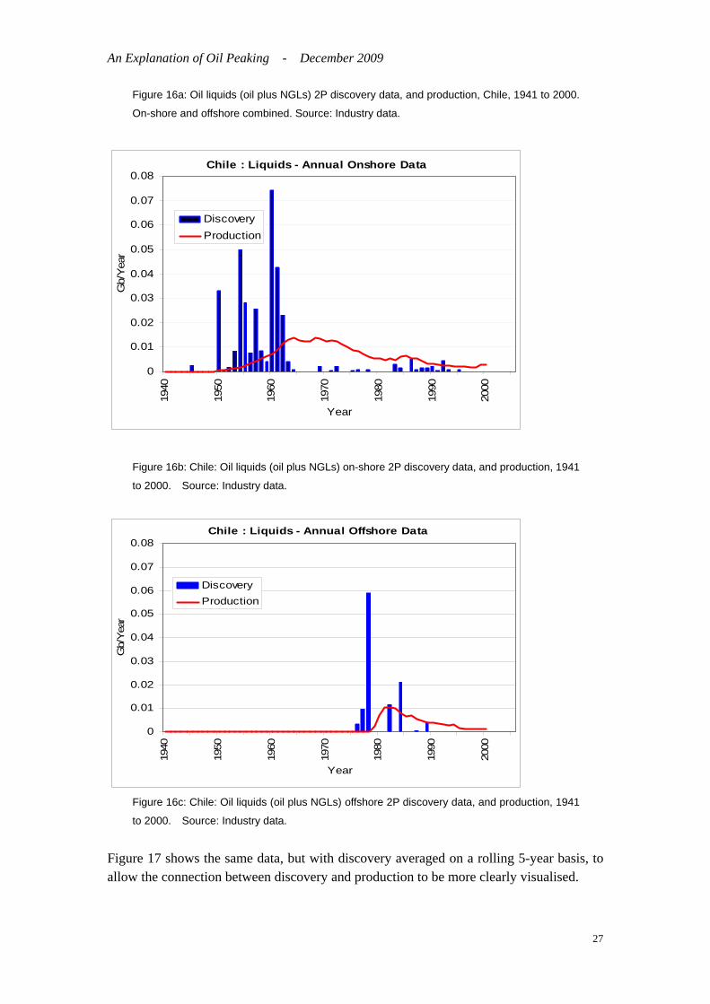
As previously, this graph poses the usual questions: - Why two peaks? - Is either peak resource-limited on the basis of discovery to-date? - Is there more oil waiting in the wings, such that a new, higher, peak will occur? And as previously, the answers have to come from the discovery trend, and from geological knowledge. Figures 16a to 16c add the 2P discovery. Figure 16a shows on-shore and offshore combined; Figures 16b and 16c show these regions separately, to make clear link between discovery and production.
26
An Explanation of Oil Peaking - December 2009
Figure 16a: Oil liquids (oil plus NGLs) 2P discovery data, and production, Chile, 1941 to 2000.
On-shore and offshore combined. Source: Industry data.
Chile : Liquids - Annual Onshore Data
0
0.01
0.02
0.03
0.04
0.05
0.06
0.07
0.0819
40
1950
1960
1970
1980
1990
2000
Year
Gb/
Yea
r
DiscoveryProduction
Figure 16b: Chile: Oil liquids (oil plus NGLs) on-shore 2P discovery data, and production, 1941
to 2000. Source: Industry data.
Chile : Liquids - Annual Offshore Data
0
0.01
0.02
0.03
0.04
0.05
0.06
0.07
0.08
1940
1950
1960
1970
1980
1990
2000
Year
Gb/
Yea
r
DiscoveryProduction
Figure 16c: Chile: Oil liquids (oil plus NGLs) offshore 2P discovery data, and production, 1941
to 2000. Source: Industry data.
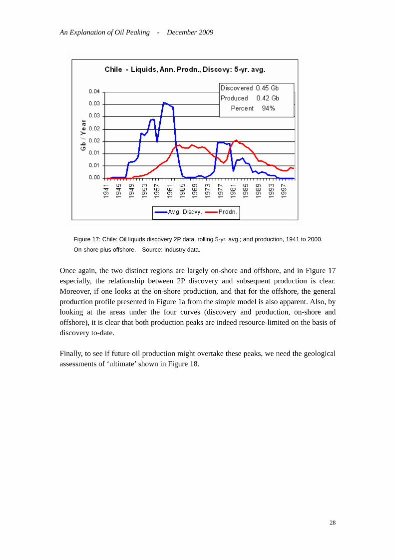
Figure 17 shows the same data, but with discovery averaged on a rolling 5-year basis, to allow the connection between discovery and production to be more clearly visualised.
27
An Explanation of Oil Peaking - December 2009
Figure 17: Chile: Oil liquids discovery 2P data, rolling 5-yr. avg.; and production, 1941 to 2000.
On-shore plus offshore. Source: Industry data.
Once again, the two distinct regions are largely on-shore and offshore, and in Figure 17 especially, the relationship between 2P discovery and subsequent production is clear. Moreover, if one looks at the on-shore production, and that for the offshore, the general production profile presented in Figure 1a from the simple model is also apparent. Also, by looking at the areas under the four curves (discovery and production, on-shore and offshore), it is clear that both production peaks are indeed resource-limited on the basis of discovery to-date. Finally, to see if future oil production might overtake these peaks, we need the geological assessments of ‘ultimate’ shown in Figure 18.
28
An Explanation of Oil Peaking - December 2009
Chile - Liquids, Cumulative data
0.00.10.20.30.40.50.60.7
1941
1946
1951
1956
1961
1966
1971
1976
1981
1986
1991
1996
2001
2006
2011
2016
2021
2026
Gb
Discovery Prodn. Peak
USGS; Mean, no RG Campbell USGS; 5% +RG
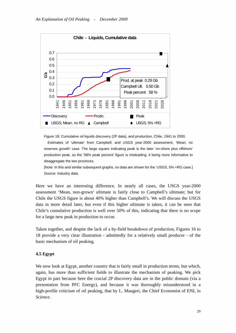
Prod. at peak 0.29 GbCampbell Ult. 0.50 Gb Peak percent 58 %
Figure 18: Cumulative oil liquids discovery (2P data), and production, Chile, 1941 to 2000.
Estimates of ‘ultimate’ from Campbell; and USGS year-2000 assessment, ‘Mean; no
reserves growth’ case. The large square indicating peak is the later ‘on-shore plus offshore’
production peak, so the ‘58% peak percent’ figure is misleading, it being more informative to
disaggregate the two provinces.
[Note: In this and similar subsequent graphs, no data are shown for the ‘USGS, 5% +RG case.]
Source: Industry data. Here we have an interesting difference. In nearly all cases, the USGS year-2000 assessment ‘Mean, non-grown’ ultimate is fairly close to Campbell’s ultimate; but for Chile the USGS figure is about 40% higher than Campbell’s. We will discuss the USGS data in more detail later, but even if this higher ultimate is taken, it can be seen that Chile’s cumulative production is well over 50% of this, indicating that there is no scope for a large new peak in production to occur. Taken together, and despite the lack of a by-field breakdown of production, Figures 16 to 18 provide a very clear illustration - admittedly for a relatively small producer - of the basic mechanism of oil peaking. 4.5 Egypt We now look at Egypt, another country that is fairly small in production terms, but which, again, has more than sufficient fields to illustrate the mechanism of peaking. We pick Egypt in part because here the crucial 2P discovery data are in the public domain (via a presentation from PFC Energy), and because it was thoroughly misunderstood in a high-profile criticism of oil peaking, that by L. Maugeri, the Chief Economist of ENI, in Science.
29
An Explanation of Oil Peaking - December 2009
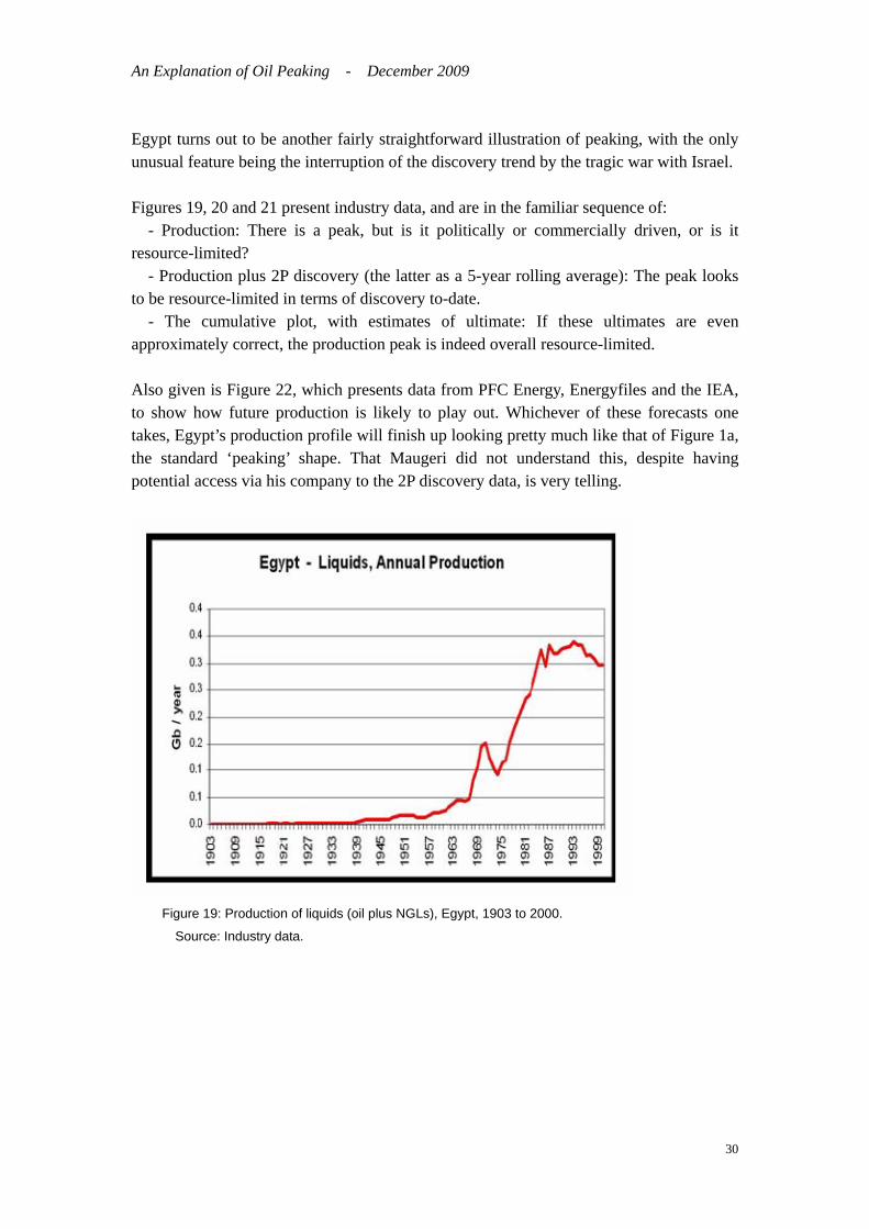
Egypt turns out to be another fairly straightforward illustration of peaking, with the only unusual feature being the interruption of the discovery trend by the tragic war with Israel. Figures 19, 20 and 21 present industry data, and are in the familiar sequence of: - Production: There is a peak, but is it politically or commercially driven, or is it resource-limited? - Production plus 2P discovery (the latter as a 5-year rolling average): The peak looks to be resource-limited in terms of discovery to-date. - The cumulative plot, with estimates of ultimate: If these ultimates are even approximately correct, the production peak is indeed overall resource-limited. Also given is Figure 22, which presents data from PFC Energy, Energyfiles and the IEA, to show how future production is likely to play out. Whichever of these forecasts one takes, Egypt’s production profile will finish up looking pretty much like that of Figure 1a, the standard ‘peaking’ shape. That Maugeri did not understand this, despite having potential access via his company to the 2P discovery data, is very telling.
Figure 19: Production of liquids (oil plus NGLs), Egypt, 1903 to 2000.
Source: Industry data.
30

An Explanation of Oil Peaking - December 2009
Figure 20: Oil liquids 2P discovery data, rolling 5-yr. avg.; and production, Egypt, 1903 to 2000.
Source: Industry data.
Figure 21: Cumulative oil liquids 2P discovery data, and production, Egypt, 1900 to 2000.
Estimates of ‘ultimate’ from Campbell; and USGS year-2000 assessment ‘Mean, no
reserves growth’ case. Large square indicates the production peak.
Sources: Discovery, production: Industry data; ‘ultimates’: see references.
31
An Explanation of Oil Peaking - December 2009
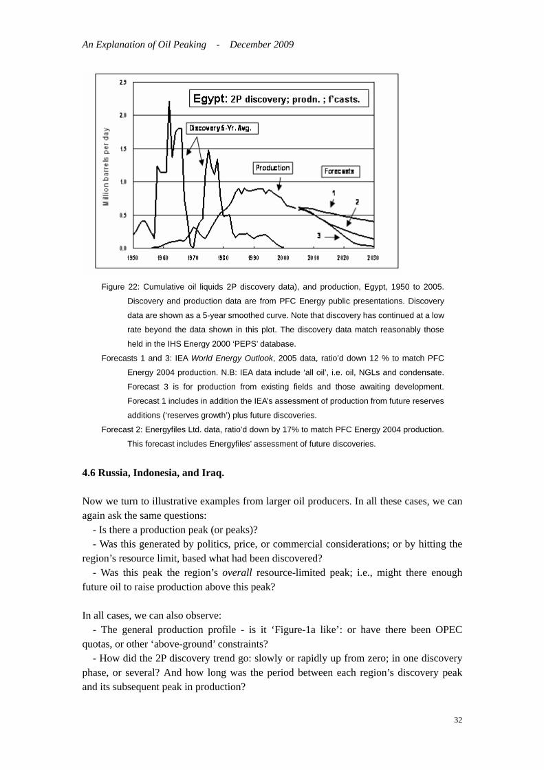
Figure 22: Cumulative oil liquids 2P discovery data), and production, Egypt, 1950 to 2005.
Discovery and production data are from PFC Energy public presentations. Discovery
data are shown as a 5-year smoothed curve. Note that discovery has continued at a low
rate beyond the data shown in this plot. The discovery data match reasonably those
held in the IHS Energy 2000 ‘PEPS’ database.
Forecasts 1 and 3: IEA World Energy Outlook, 2005 data, ratio’d down 12 % to match PFC
Energy 2004 production. N.B: IEA data include ‘all oil’, i.e. oil, NGLs and condensate.
Forecast 3 is for production from existing fields and those awaiting development.
Forecast 1 includes in addition the IEA’s assessment of production from future reserves
additions (‘reserves growth’) plus future discoveries.
Forecast 2: Energyfiles Ltd. data, ratio’d down by 17% to match PFC Energy 2004 production.
This forecast includes Energyfiles’ assessment of future discoveries. 4.6 Russia, Indonesia, and Iraq. Now we turn to illustrative examples from larger oil producers. In all these cases, we can again ask the same questions: - Is there a production peak (or peaks)? - Was this generated by politics, price, or commercial considerations; or by hitting the region’s resource limit, based what had been discovered? - Was this peak the region’s overall resource-limited peak; i.e., might there enough future oil to raise production above this peak? In all cases, we can also observe: - The general production profile - is it ‘Figure-1a like’: or have there been OPEC quotas, or other ‘above-ground’ constraints? - How did the 2P discovery trend go: slowly or rapidly up from zero; in one discovery phase, or several? And how long was the period between each region’s discovery peak and its subsequent peak in production?
32

An Explanation of Oil Peaking - December 2009
Because you, dear reader, may now be rather bored with the topic (like this writer’s long-suffering friends), there will not be much comment in each case; and you can draw your own by now rather well-educated judgements on the answers to the above questions. The countries examined are Russia, Indonesia and Iraq. (a). Russia, Figures 23, 24a and 24b. - The drop-off in both discovery and production due to the collapse of the Soviet Union is clear. - The Campbell ultimate, as of the date of this plot, in Figure 24a was significantly lower than the apparent 2P discovery. This is because Campbell here excludes polar oil, and also judges that much of the Russia reserves data in fact to be 3P. - Even though up to very recently many analysts were predicting that Russia would come to the rescue of the West with large increases in future production, it is clear from the 2P discovery data that for conventional oil at least she is close to, or past, her ‘mid-point’, so any future production gains cannot be large, nor last for long. (One view of this is given in Figure 24b).
Figure 23: Oil liquids (oil plus NGLs) 2P discovery data, and production, Russia, 1900 to 2000.
Source: Industry data.
33

An Explanation of Oil Peaking - December 2009
Figure 24a: Cumulative oil liquids 2P discovery data, and production, Russia, 1900 to 2000.
Estimates of ‘ultimate’ from Campbell; and USGS year-2000 assessment ‘Mean, no reserves
growth’ case. Source: Industry data.
Russia crude oil & liquids production for an ultimate 250 Gb
0
2
4
6
8
10
12
1930 1940 1950 1960 1970 1980 1990 2000 2010 2020 2030 2040 2050
year
crude oilliquids CP07=152 GbU=250 Gb
Jean Laherrere 2008
Figure 24b: Jean Laherrère’s view of possible future Russian oil production, based on a URR
of 250 Gb. Source: Laherrère.
34
An Explanation of Oil Peaking - December 2009
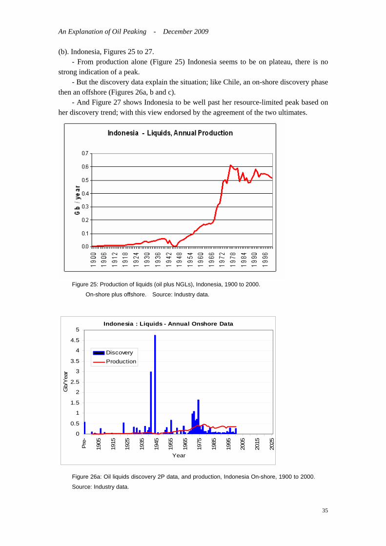
(b). Indonesia, Figures 25 to 27. - From production alone (Figure 25) Indonesia seems to be on plateau, there is no strong indication of a peak. - But the discovery data explain the situation; like Chile, an on-shore discovery phase then an offshore (Figures 26a, b and c). - And Figure 27 shows Indonesia to be well past her resource-limited peak based on her discovery trend; with this view endorsed by the agreement of the two ultimates.
Figure 25: Production of liquids (oil plus NGLs), Indonesia, 1900 to 2000.
On-shore plus offshore. Source: Industry data.
Indonesia : Liquids - Annual Onshore Data
0
0.5
1
1.5
2
2.5
3
3.5
4
4.5
5
Pre
-
1905
1915
1925
1935
1945
1955
1965
1975
1985
1995
2005
2015
2025
Year
Gb/
Yea
r
DiscoveryProduction
Figure 26a: Oil liquids discovery 2P data, and production, Indonesia On-shore, 1900 to 2000.
Source: Industry data.
35

An Explanation of Oil Peaking - December 2009
Indonesia : Liquids - Annual Offshore Data
0
0.5
1
1.5
2
2.5
Pre
-
1905
1915
1925
1935
1945
1955
1965
1975
1985
1995
2005
2015
2025
Year
Gb/
Yea
r
DiscoveryProduction
Figure 26b: Oil liquids discovery 2P data, and production, Indonesia Offshore, 1900 to 2000.
Source: Industry data.
Figure 26c: Oil liquids discovery 2P data, rolling 5-yr. avg.; and production, Indonesia, 1900 to
2000. On-shore plus offshore. Source: Industry data.
36

An Explanation of Oil Peaking - December 2009
Figure 27: Cumulative oil liquids discovery (2P data), and production, Indonesia, 1900 to 2000.
On-shore plus offshore. Estimates of ‘ultimate’ from Campbell; and USGS year-2000
assessment ‘Mean, no reserves growth’ case. Large square indicates the production peak.
Sources: Discovery, production: Industry data; ‘ultimates’: see text.
(c). Iraq, Figures 28 and 29. - Three phases of discovery (roughly, Kirkuk, Rumailia, and East Baghdad); raising the question: Is there a lot more oil to discover? Many analysts look to the Western desert to yield much. But the USGS, presumably to help plans for the country’s reconstruction, were asked to re-visit their year-2000 assessment in greater detail. They looked very thoroughly at source rocks, traps, and possible migration paths; but stuck more-or-less to their year-2000 assessment of ultimate. This, as Figure 29 shows, for the mean ‘non-grown’ value, is close to Campbell’s estimate of ultimate. Therefore, though Iraq is unlikely to have much more oil than already discovered, this is still a considerable amount, of which only relatively little has been used (Figure 29), so can support the country’s development for many years to come.
37
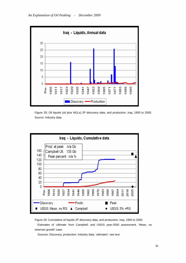
An Explanation of Oil Peaking - December 2009
Figure 28: Oil liquids (oil plus NGLs) 2P discovery data, and production, Iraq, 1900 to 2000.
Source: Industry data.
Figure 29: Cumulative oil liquids 2P discovery data, and production, Iraq, 1900 to 2000.
Estimates of ‘ultimate’ from Campbell; and USGS year-2000 assessment, ‘Mean, no
reserves growth’ case.
Sources: Discovery, production: Industry data; ‘ultimates’: see text.
38

An Explanation of Oil Peaking - December 2009
4.7 Saudi Arabia Now we turn to Saudi Arabia. As Figures 30 and 31a show, this country is fairly straightforward in terms of its patterns of discovery and production. There is some disagreement however - indeed, true uncertainty - on what is the country’s realistic ultimate, see Figure 31a. Despite the views of a few authors, there exists relatively little uncertainty on the size of future discoveries. These are generally taken as fairly small due to the region’s specific petroleum geology of large salt-sealed anticlines. As a result - despite the low number of exploration wells to-date - the apparent discovery asymptote is clearly visible in Figure 31a. This is supported by the USGS’ detailed year-2000 analysis. Instead, the uncertainty on the size of the ultimate hinges on the quantity of 2P oil already discovered; where some authorities take a higher figure, and some, such as Campbell, a lower. (Laherrère notes that IHS Energy is now obliged to report Saudi Aramco reserves estimates, whereas previously there were no official estimates and Petroconsultants, IHS Energy’s predecessor company, reported much lower numbers. IHS Energy’s cumulative discoveries for Saudi Arabia stand now at about 400 Gb, in agreement, therefore, with the country’s reported remaining reserves of 264 Gb.)
Figure 30: Oil liquids (oil plus NGLs) 2P discovery data, and production, Saudi Arabia, 1900 to
2000. Source: Industry data.
39

An Explanation of Oil Peaking - December 2009
Figure 31a: Cumulative oil liquids 2P discovery data, and production, Saudi Arabia, 1900 to
2000. Estimates of ‘ultimate’ from Campbell; and USGS year-2000 assessment ‘Mean, no
reserves growth’ case.
Sources: Discovery, production: Industry data; ‘ultimates’: see text.
Although this paper has primarily set out to explain peaking, and not to offer forecasts, for Saudi Arabia we will present a number of forecasts. The reason is that several people, including, for example, Adnan Shihab-Eldin, have questioned the validity of the simple model of Section 2 in the more complex case of the Middle East producers. This is a sensible question as there are indeed significant differences between countries like the UK, where the ‘simple model’ captures the main drivers of the peak, and the large Middle East suppliers. In the latter, unlike in, say, the UK: - There is usually one, or a small number of, extremely large fields, and then a succession of smaller, more typically distributed fields in terms of size. - The one, or few, extremely large fields have normally been held on-plateau; but also, from time to time, seen wide production excursions resulting from OPEC quotas and other considerations. - Some of these countries, Saudi Arabia especially, have considerable oil in fallow fields waiting to come on-stream once the extremely large fields go into decline. - Since expropriation, exploration expenditure and field upgrades in these countries has had to be paid for in real money; not in tax-deductible ‘10-cents-on-the-dollar’ money when the oil companies were in control. So the question is: Can we apply the lessons drawn above from countries already past
40

An Explanation of Oil Peaking - December 2009
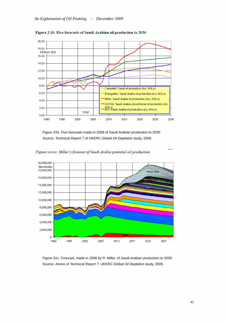
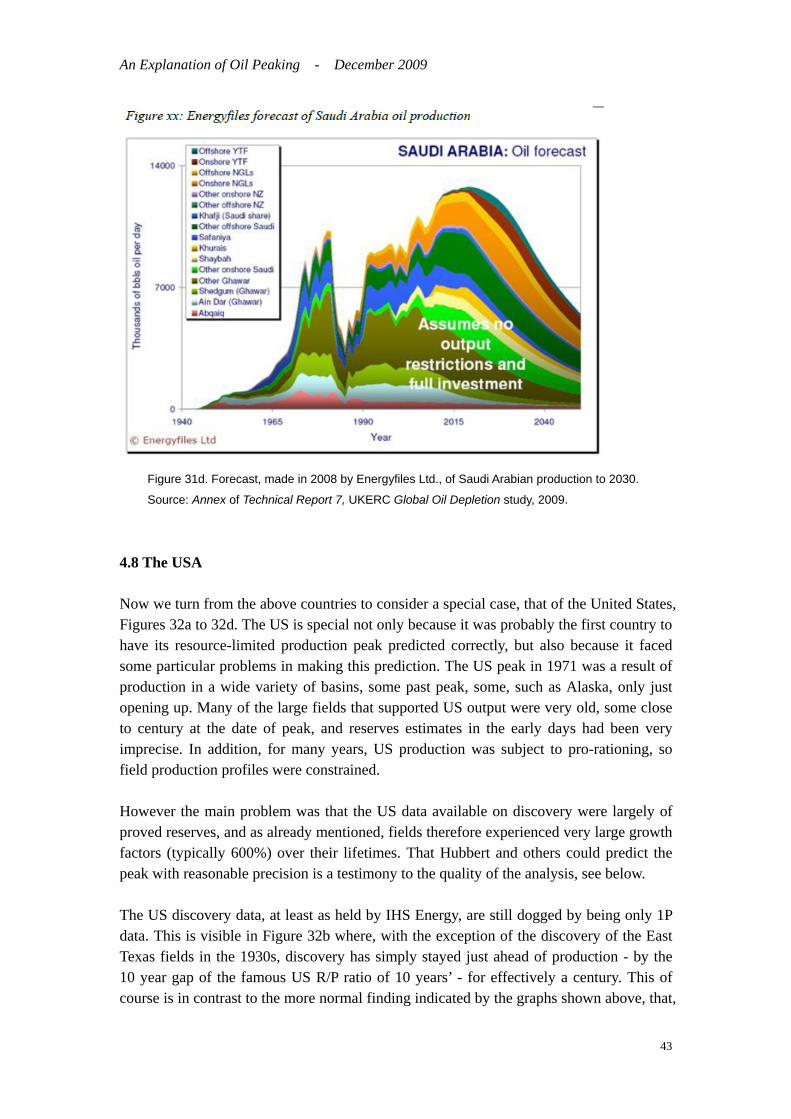
peak to the big Middle East producers? To answer this, we look at current forecasts for Saudi Arabian production, given in Figures 31b to 31d below. Figure 31b is taken from Technical Report 7 of the recent UK Energy Research Centre (UKERC) report on Global Oil Depletion (see www.ukerc.ac.uk). The figure shows the results from five forecasts made in 2008 for Saudi Arabian output to 2030. As can be seen, two of the forecasts (from the IEA and the US EIA) show no peak in production before 2030, the other three indicate a peak. We can look at this more closely by examining the forecasts that indicate peak. The Campbell forecast is based on the assumption that Saudi Arabian reserves are significantly over-stated. This is a contentious topic. Miller’s forecast, Figure 31c, is bottom-up by field, and includes his view of Saudi Arabian reserves, yet-to-find and likely reserves growth. It shows the ‘Miller bump’ in production that would occur if the country’s fallow fields were brought on-stream almost immediately. Miller shows this case, but reports that he thinks it very unlikely. Energyfiles’ forecast, Figure 31d, also bottom-up by field, seems to take this more pessimistic view of the fallow fields production. On the basis, one can see that the IEA and US EIA forecasts are not impossible, given the oil present in the fallow fields, but both would require - if the evaluations of Miller and Energyfiles of available oil are roughly correct - that total Saudi Arabian production peaks soon after 2030. Of particular importance for Saudi Arabian production is the behaviour of the country’s largest field, Ghawar. This has reportedly seen excellent production work in terms of water injection wells along the field flanks, and one reservoir engineer familiar with the field suggests that production will ‘go out like a light’ at the end of this injection phase. However, the field is far from homogenous along its length, and both Miller and Energyfiles indicate instead that Ghawar’s production will tail off over time in a typical exponential fashion. However, the main purpose for showing these by-field forecasts of Miller and Energyfiles is to indicate that the mechanism of resource-limited oil peaking - the result of adding the output from large early fields, and then from smaller fields - is expected to operate in the same fundamental way for the large Middle East producers as for countries already past peak, such as the UK.
41
An Explanation of Oil Peaking - December 2009
Figure 31b. Five forecasts made in 2008 of Saudi Arabian production to 2030.
Source: Technical Report 7 of UKERC Global Oil Depletion study, 2009.
Figure 31c. Forecast, made in 2008 by R. Miller, of Saudi Arabian production to 2030.
Source: Annex of Technical Report 7, UKERC Global Oil Depletion study, 2009.
42
An Explanation of Oil Peaking - December 2009
Figure 31d. Forecast, made in 2008 by Energyfiles Ltd., of Saudi Arabian production to 2030.
Source: Annex of Technical Report 7, UKERC Global Oil Depletion study, 2009. 4.8 The USA Now we turn from the above countries to consider a special case, that of the United States, Figures 32a to 32d. The US is special not only because it was probably the first country to have its resource-limited production peak predicted correctly, but also because it faced some particular problems in making this prediction. The US peak in 1971 was a result of production in a wide variety of basins, some past peak, some, such as Alaska, only just opening up. Many of the large fields that supported US output were very old, some close to century at the date of peak, and reserves estimates in the early days had been very imprecise. In addition, for many years, US production was subject to pro-rationing, so field production profiles were constrained. However the main problem was that the US data available on discovery were largely of proved reserves, and as already mentioned, fields therefore experienced very large growth factors (typically 600%) over their lifetimes. That Hubbert and others could predict the peak with reasonable precision is a testimony to the quality of the analysis, see below. The US discovery data, at least as held by IHS Energy, are still dogged by being only 1P data. This is visible in Figure 32b where, with the exception of the discovery of the East Texas fields in the 1930s, discovery has simply stayed just ahead of production - by the 10 year gap of the famous US R/P ratio of 10 years’ - for effectively a century. This of course is in contrast to the more normal finding indicated by the graphs shown above, that,
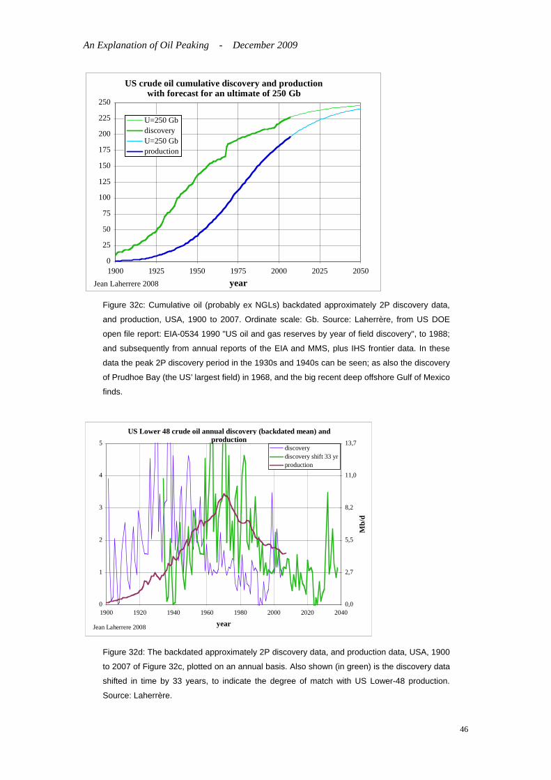
43

An Explanation of Oil Peaking - December 2009
even for regions with a number of basins, discovery usually rises steeply and then tends towards asymptote, while production usually follows a more ‘S’-shaped curve, approximating the logistic function. In the US, the difference between 2P discovery and the 1P ‘apparent discovery’ is significant. As Figure 32a indicates, 1P ‘discovery’ reached a maximum in the period between about 1960 to 1990; whereas the 2P discovery data, as Hubbert and others had shown, indicated that the peak of ‘real’ (proved plus probable) US discovery was much earlier, back in the 1930s. This is borne out by Figure 32c. This shows data provided by Jean Laherrère taken from the US DOE EIA open file report EIA-0534 1990 "US oil and gas reserves by year of field discovery" up to 1988; and using data since then from EIA and MMS annual reports, as well IHS frontier data. On the basis of the discovery trend shown by these data (compare Figure 32c with 32b), Laherrère assumes that these data approximate true backdated 2P data. And, of course, it was the fact that US ‘proved plus probable’ discovery had long been in decline by 1971 which indicated that this peak was indeed - for conventional oil - resource-limited. This is indicated by Laherrère’s analysis of the above approximate 2P discovery data given in Figure 32d. Hubbert particularly, and later Ivanhoe and Laherrère, made use of the fairly constant time period (albeit, individual to each country) between discovery & production as one approach to forecast peak. Nevertheless, for Hubbert and others having to create the US ‘2P discovery’ data by ‘growing’ reserves - rather than having these already tabulated - was a major added difficulty in predicting the date of peak.
44

An Explanation of Oil Peaking - December 2009
Figure 32a: Oil liquids (oil plus NGLs) proved (1P) discovery data, and production, USA, 1900
to 2000. The discovery of the US’ largest field, Prudhoe Bay in 1968 is visible. Also apparent,
as these are ‘1P’ discovery’ data, is the close match in timing between ‘discovery’ (meaning the
classification of already discovered oil as proved) - and subsequent production. Source: IHS
Energy, with permission.
Figure 32b: Cumulative oil liquids (incl. NGLs) ‘proved (1P) discovery’ data, and production,
USA, 1900 to 2000. The US’ famous 10-year gap between ‘proved discovery’ and production,
reflecting the decades-long virtually constant R/P ratio of proved reserves to production of 10
years, is clear.
Also shown are three estimates of the US conventional oil ‘ultimate’ ; that from Campbell;
and two USGS year-2000 assessment ultimates; the ‘Mean, no reserves growth’ case; and the
‘5% probable plus reserves growth’ case. Campbell’s ultimate is for ‘regular oil’, so excludes
the polar oil of Prudhoe Bay and other Alaskan fields, as well as deepwater GoM fields.
Because the ‘discovery’ data are 1P, there is no very obvious flattening out of discovery
towards an asymptote (as is the case with the US’ 2P discovery trend, see Hubbert’s
publications; and Figure 32c), so it is not possible from these data to assess which ultimate is
most likely.
The large square indicates the production peak; at which point just over 100 Gb (including
NGLs) had been produced.
Sources: Discovery, production: IHS Energy, with permission; ‘ultimates’: see text.
45
An Explanation of Oil Peaking - December 2009
US crude oil cumulative discovery and production
with forecast for an ultimate of 250 Gb
0
25
50
75
100
125
150
175
200
225
250
1900 1925 1950 1975 2000 2025 2050year
U=250 Gbdiscovery U=250 Gbproduction
Jean Laherrere 2008
Figure 32c: Cumulative oil (probably ex NGLs) backdated approximately 2P discovery data,
and production, USA, 1900 to 2007. Ordinate scale: Gb. Source: Laherrère, from US DOE
open file report: EIA-0534 1990 "US oil and gas reserves by year of field discovery", to 1988;
and subsequently from annual reports of the EIA and MMS, plus IHS frontier data. In these
data the peak 2P discovery period in the 1930s and 1940s can be seen; as also the discovery
of Prudhoe Bay (the US’ largest field) in 1968, and the big recent deep offshore Gulf of Mexico
finds.
US Lower 48 crude oil annual discovery (backdated mean) and
production
0
1
2
3
4
5
1900 1920 1940 1960 1980 2000 2020 2040
year
0,0
2,7
5,5
8,2
11,0
13,7
Mb/
d
discoverydiscovery shift 33 yrproduction
Jean Laherrere 2008
Figure 32d: The backdated approximately 2P discovery data, and production data, USA, 1900
to 2007 of Figure 32c, plotted on an annual basis. Also shown (in green) is the discovery data
shifted in time by 33 years, to indicate the degree of match with US Lower-48 production. Source: Laherrère.
46

An Explanation of Oil Peaking - December 2009
Given the importance of the US in the development of methods for predicting when production in region will peak, and because aspects of the general approach are often still only poorly understood, these are presented briefly here in the context of Figures 33a to 33d. The first thing to note is that Hubbert and others working in the field at the time had plenty of evidence of regions where production was in decline. Figure 33a shows some of the individual US States for which this is now true. Today, the majority of all US oil-producing states, including Alaska, are in decline. (This is not, of course, to say that all are necessarily past peak. As explained above, to know with some confidence that a region is past peak one needs to see that 2P discovery has long been in decline, and, in addition, to have a geological assessment that there are unlikely to be large new recoverable resources waiting to be discovered.)
Pennsylvania
0
5,000
10,000
15,000
20,000
25,000
1918192
2192
6193
0193
4193
8194
2194
6195
0195
4195
8196
2196
6197
0197
4197
8198
2198
6199
0199
4199
8200
2200
6
Prod
uctio
n ('00
0 bbls
)
Virginia
0
1,000
2,000
3,000
4,0005,000
6,000
7,000
8,000
9,000
1918
1922192
6193
0193
4193
8194
2194
6195
0195
4195
8196
2196
6197
0197
4197
8198
2198
6199
0199
4199
8200
2200
6
Prod
uctio
n ('00
0 bbls
)
Oklahoma
0
50,000
100,000
150,000
200,000
250,000
300,000
1918192
2192
6193
0193
4193
8194
2194
6195
0195
4195
8196
2196
6197
0197
4197
8198
2198
6199
0199
4199
8200
2200
6
Prod
uctio
n ('00
0 bbls
/yr.)
Texas
0
200,000
400,000
600,000
800,000
1,000,000
1,200,000
1,400,000
1918
1922
1926
1930
1934
1938
1942
1946
1950
1954
1958
1962
1966
1970
1974
1978
1982
1986
1990
1994
1998
2002
2006
Prod
uctio
n ('00
0 bbls
/yr.)
US states: 1918-2007. B. of Mines & EIA - DeGolyer & MacNaughton
Figure 33a. Examples of US states where production is in decline. This is now true for
production from most US oil-producing states, including Alaska. Source: US Bureau of Mines
and EIA, from DeGolyer & MacNaughton.
If one adds the output from the US States, total production is as shown in Figure 33b. And if only the Lower-48 states are included, as Hubbert explicitly modelled, production is as in Figure 33c.
47

An Explanation of Oil Peaking - December 2009
0
5 0 0 ,0 0 0
1 ,0 0 0 ,0 0 0
1 ,5 0 0 ,0 0 0
2 ,0 0 0 ,0 0 0
2 ,5 0 0 ,0 0 0
3 ,0 0 0 ,0 0 0
3 ,5 0 0 ,0 0 0
4 ,0 0 0 ,0 0 0
1918
1923
1928
1933
1938
1943
1948
1953
1958
1963
1968
1973
1978
1983
1988
1993
1998
2003
An
nu
al P
rod
uc
tion
('00
0
GoM Fe d O f f s h .
A la s ka
Pac . Fed O f f .
Nev ada
Calif o rn ia
W y oming
Uta h
Montana
Colorad o
Tex as
New Mex ic o
Mis s is s ip p i
Lou is ana ad j.
A rka ns as
A la bama
Tenes s ee
S. Dako ta
Oklahoma
Ohio
N. Dako ta
Nebras ka
Mis s our i
Mic h ig an
Kentuc ky
Kans as
Ind iana
Illino is
V irg in ia
Penns y lv an ia
New Y ork
Flor ida
US production 1918-2007 – Data B. Mines & EIA – DeGoyler & MacNaughton
Figure 33b. US production summed by state, 1918 - 2007. Excludes NGLs. Source: DeGolyer
& MacNaughton.
US Lower-48 Production
0
500,000
1,000,000
1,500,000
2,000,000
2,500,000
3,000,000
3,500,000
4,000,000
1918
1923
1928
1933
1938
1943
1948
1953
1958
1963
1968
1973
1978
1983
1988
1993
1998
2003
Ann
ual P
rodu
ctio
n ('0
00 b
bls)
Nevada
California
Wyoming
Utah
Montana
Colorado
Texas
New Mexico
Mississippi
Louisana adj.
Arkansas
Alabama
Tenessee
S. Dakota
Oklahoma
Ohio
N. Dakota
Nebraska
Missouri
Michigan
Kentucky
Kansas
Indiana
Illinois
Virginia
Pennsylvania
New York
Florida
Figure 33c. US Lower-48 production summed by state. Excludes NGLs. It was specifically for
the Lower-48 oil (excluding NGLs) that Hubbert did his forecasting, and for which the initial two
1956 estimates of ultimate, of 150 Gb and 200 Gb, were provided by industry analysts.
(Subsequent analyses by Hubbert, using a wide variety of methods, arrived at estimates for US
Lower-48 ultimate mostly in the region of 175 - 180 Gb.) Data source: DeGolyer &
MacNaughton.
48
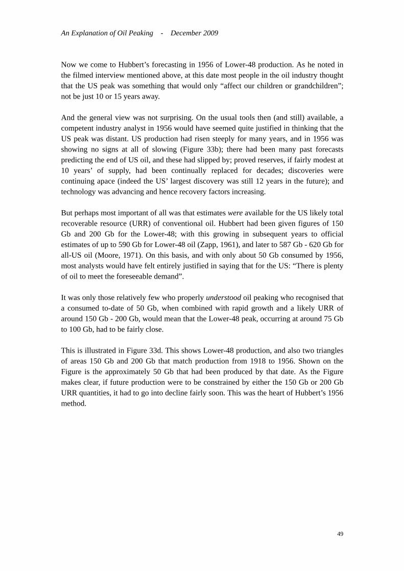
An Explanation of Oil Peaking - December 2009
Now we come to Hubbert’s forecasting in 1956 of Lower-48 production. As he noted in the filmed interview mentioned above, at this date most people in the oil industry thought that the US peak was something that would only “affect our children or grandchildren”; not be just 10 or 15 years away. And the general view was not surprising. On the usual tools then (and still) available, a competent industry analyst in 1956 would have seemed quite justified in thinking that the US peak was distant. US production had risen steeply for many years, and in 1956 was showing no signs at all of slowing (Figure 33b); there had been many past forecasts predicting the end of US oil, and these had slipped by; proved reserves, if fairly modest at 10 years’ of supply, had been continually replaced for decades; discoveries were continuing apace (indeed the US’ largest discovery was still 12 years in the future); and technology was advancing and hence recovery factors increasing. But perhaps most important of all was that estimates were available for the US likely total recoverable resource (URR) of conventional oil. Hubbert had been given figures of 150 Gb and 200 Gb for the Lower-48; with this growing in subsequent years to official estimates of up to 590 Gb for Lower-48 oil (Zapp, 1961), and later to 587 Gb - 620 Gb for all-US oil (Moore, 1971). On this basis, and with only about 50 Gb consumed by 1956, most analysts would have felt entirely justified in saying that for the US: “There is plenty of oil to meet the foreseeable demand”. It was only those relatively few who properly understood oil peaking who recognised that a consumed to-date of 50 Gb, when combined with rapid growth and a likely URR of around 150 Gb - 200 Gb, would mean that the Lower-48 peak, occurring at around 75 Gb to 100 Gb, had to be fairly close. This is illustrated in Figure 33d. This shows Lower-48 production, and also two triangles of areas 150 Gb and 200 Gb that match production from 1918 to 1956. Shown on the Figure is the approximately 50 Gb that had been produced by that date. As the Figure makes clear, if future production were to be constrained by either the 150 Gb or 200 Gb URR quantities, it had to go into decline fairly soon. This was the heart of Hubbert’s 1956 method.
49

An Explanation of Oil Peaking - December 2009
US Lower - 48: Showi ng Act ual Oi l Pr oduct i on andFor ecast s f or 1956 f or URR = 150 Gb; and = 200 Gb.
0
1
2
3
4
5
6
7
8
9
1019
18
1926
1934
1942
1950
1958
1966
1974
1982
1990
1998
2006
Prod
ucti
on (
Mb/d
ay)
If URR = 200 Gb,Remaining = 150 Gb
If URR = 150 Gb,Remaining = 100 Gb
Production: 50 Gb
1956
Figure 33d. Showing how Hubbert combined approximate ‘mid-point peaking’ with two
industry-provided estimates of US Lower-48 conventional oil ultimately recoverable reserves
(URR), excluding NGLs, to predict US production beyond 1956.
- The red triangle indicates a URR of volume 150 Gb; the extension of the purple triangle a
URR volume of 200 Gb.
- By 1956, the US had produced about 50 Gb, indicated by the volume under the red triangle
up to 1956 cut-off line.
- The triangles show how future production, if it were to continue on the same upward
trajectory, but also peak at mid-point and total no more than the URR, then had to peak around
1965 for the URR of 150 Gb, and around 1970 for the URR of 200 Gb.
- In his paper, Hubbert did not use a triangular production profile (used here for simplicity),
but hand-drew a production curve of roughly the profile of Figure 1a.
As the Figure indicates, and as Hubbert noted in 1956, once the produced-to-date and the
URR quantities had been identified, there was little scope for US production to peak at dates
much different from those he indicated. By contrast, without an appreciation of mid-point
peaking, a produced-to-date of 50 Gb and a URR of 150 Gb (let alone 200 Gb) would alert few
to an imminent peak in production. In the event, Hubbert’s later estimates for the US Lower-48
ultimate, of between about 175 and 180 Gb, look accurate, not only in terms of the date of peak,
but also in the path mapped out since by nearly 40 further years of Lower-48 production. Kaufmann and Cleveland (2001) could later write “In effect, Hubbert got lucky” in his predicted date for the US peak; and technically this is probably true in terms of the impacts of pro-rationing rules, oil price and so on. But as Figure 33d shows very clearly, Hubbert was correct to say that given the constraints of the consumed to-date and the likely URR quantities, he had very little freedom to draw a realistic future production
50
An Explanation of Oil Peaking - December 2009
profile (approximately the profile of Figure 1a) that did not peak around the dates he indicated; about 1965 for the lower URR estimate, and around 1970 for the higher. The lesson, therefore, from the US - just as from the simple model, and from the UK - is that the date of the production peak is easy to estimate with some precision provided one has an understanding of ‘mid-point peaking’, and a fairly realistic estimate for the URR. In the event, the US peak produced serious consequences. Prior to this, OPEC had tried on a number of occasions to restrict production in order to obtain what it felt was a fairer share of the oil price, but each time had been stymied by the US foregoing pro-rationing, and opening up the taps. Post the US peak, this was not an option and the oil price shocks of 1973 and 1978 resulted. Many other things followed in their train, including; inflation, stagflation, unemployment, and significant third-world debt (as mineral-rich but governance-poor countries were encouraged to take on loans to recycle petrodollars). But good things happened also, the IEA was set up, research into renewable energies burgeoned, and OPEC learned that too high a price would push its customers into recession, and also erode currencies and hence the real price it received for its oil. These are all important lessons this time around. 4.9 General conclusions from countries past peak We have now looked at data from 12 countries. Many more examples could be given; indeed the data on discovery and production for all countries are fascinating, and all countries have a story to tell. Nearly all regions show clearly how 2P discovery sets the limit on subsequent production. And, as mentioned earlier, discovery trend data plus geological knowledge - the latter often encapsulated in the estimate of ‘ultimate’ - show that over sixty countries, out of the world’s a hundred or so oil producing countries, are now past their overall resource-limited peak in the production of conventional oil. Figure 34a, from the German consultancy LBST, indicates the production profiles and peak dates of some of these.
51
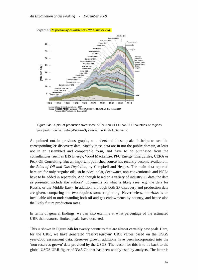
An Explanation of Oil Peaking - December 2009
Figure 34a: A plot of production from some of the non-OPEC non-FSU countries or regions
past peak. Source. Ludwig-Bölkow-Systemtechnik GmbH, Germany.
As pointed out in previous graphs, to understand these peaks it helps to see the corresponding 2P discovery data. Mostly these data are in not the public domain, at least not in an assembled and comparable form, and have to be purchased from the consultancies, such as IHS Energy, Wood Mackenzie, PFC Energy, Energyfiles, CERA or Peak Oil Consulting. But an important published source has recently become available in the Atlas of Oil and Gas Depletion, by Campbell and Heapes. The main data reported here are for only ‘regular oil’, so heavies, polar, deepwater, non-conventionals and NGLs have to be added in separately. And though based on a variety of industry 2P data, the data as presented include the authors’ judgements on what is likely (see, e.g. the data for Russia, or the Middle East). In addition, although both 2P discovery and production data are given, comparing the two requires some re-plotting. Nevertheless, the Atlas is an invaluable aid to understanding both oil and gas endowments by country, and hence also the likely future production rates. In terms of general findings, we can also examine at what percentage of the estimated URR that resource-limited peaks have occurred. This is shown in Figure 34b for twenty countries that are almost certainly past peak. Here, for the URR, we have generated ‘reserves-grown’ URR values based on the USGS year-2000 assessment data. Reserves growth additions have been incorporated into the ‘non-reserves-grown’ data provided by the USGS. The reason for this is to tie back to the global USGS URR figure of 3345 Gb that has been widely used by analysts. The latter is
52

An Explanation of Oil Peaking - December 2009
the year-2000 ‘oil plus NGLs’ total URR assessment for the world including the US, and including reserves growth. The data in Figure 34b indicate that the ‘percentage of URR produced at peak’ is variable. However, the main lesson from the Figure is to caution that if this ‘reserve-grown’ URR is used, countries generally go past their resource-limited production peak well before the URR mid-point. That is, a ‘high’ global URR of 3345 Gb - if correct - gives potential security that this amount of oil can be accessed over time; but gives no security about the distance away of the production peak.
0
50
100
150
200
250
300
350
400
Arge
nti n
a
Mal a
ysi a
Oman
Egyp
t
Col o
mbi a
Aust
r al i
a UK
I ndo
nesi
a
Norw
ay
Mexi
co USA
Gb
0%
10%
20%
30%
40%
50%
60%
Pr e- Peak Post - peak % URR at Peak
0
1
2
3
4
5
6
7
8
9
10
Fran
ce
Net h
erl a
nds
Tur k
ey
Denm
ark
Germ
any
Came
r oon
T. &
Tob
ago
Per u
Roma
nia
Gb
0%
10%
20%
30%
40%
50%
60%
Pr e- peak Post - peak % URR at Peak
Figure 34b: Plots indicating, for different countries, the percentage of the estimated
‘reserves-grown’ URR at which the resource-limited production peak occurred. Top graph is for
53
An Explanation of Oil Peaking - December 2009
countries past peak having relatively large URRs; lower graph for countries past peak with
lower URRs. Note that the USGS year-2000 study evaluated reserves growth globally, but did
not ascribe to countries. To generate these graphs, the data for the US have been taken from
the assessment’s Table AR-1; while USGS global-average ratios of reserves growth for oil, and
for NGLs, have been applied to the USGS oil and NGL data given in Table AR-9 for the
assessed countries. In the graphs, oil and NGLs have been added.
The graphs show that the percentage of ‘reserves-grown URR’ produced at the point of
resource-limited peak is variable, but is mainly in the range 25% - 35% for smaller countries,
and 25% - 45% for larger countries.
The key point is that if a large ‘reserves-grown’ URR is being considered for a country, then the
country’s resource-limited production peak should be expected well before 50% of this URR
has been produced.
4.10 The World Finally let us turn to plots of 2P discovery and production for the World as a whole, Figures 35a to 35c. - In Figure 35a, the years in which the East Texas, Burgan and Ghawar fields were found all stand out; as does the prolific discovery period from 1960 to 1980 when digital seismic came into its own. Even so, the World’s peak of discovery occurred back in the 1960s; and about 1980 was the critical date when global production overtook discovery of oil in new fields (i.e., excluding reserves growth in existing fields). - Figure 35b shows that for conventional oil the world has now used about half the amount indicated by the asymptote of the 2P discovery trend; i.e. is at the point at which peak is expected if the ‘mid-point rule’ is applied. Looking carefully at this plot, one can see that the date of World peak - for conventional oil - could be predicted by extrapolation with some confidence from about 1970. This is not surprising, as the peak in 2P discovery in the 1960s allowed the World ultimate to be estimated fairly securely from about that date (see Figure 7 for the analogous situation in terms of predicting the UK peak).
54

An Explanation of Oil Peaking - December 2009
Figure 35a: Oil liquids (oil plus NGLs) 2P discovery data (except US and Canada, which are
1P), and production, World, 1900 to 2000.
The discovery years of the East Texas, Burgan (Kuwait) and Ghawar (Saudi Arabia) fields
stand out. Peak 2P discovery was in the mid-1960s. Production first exceeded new-field
discovery about 1980. Source: IHS Energy, with permission.
Figure 35b: Cumulative oil liquids 2P discovery data (except US and Canada, which are 1P
data), and production, World, 1900 to 2000.
55
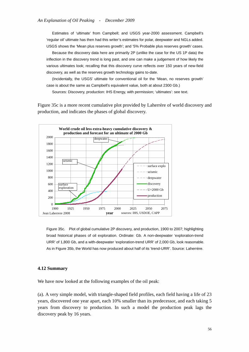
An Explanation of Oil Peaking - December 2009
Estimates of ‘ultimate’ from Campbell; and USGS year-2000 assessment. Campbell’s
‘regular oil’ ultimate has then had this writer’s estimates for polar, deepwater and NGLs added.
USGS shows the ‘Mean plus reserves growth’; and ‘5% Probable plus reserves growth’ cases.
Because the discovery data here are primarily 2P (unlike the case for the US 1P data) the
inflection in the discovery trend is long past, and one can make a judgement of how likely the
various ultimates look; recalling that this discovery curve reflects over 150 years of new-field
discovery, as well as the reserves growth technology gains to-date.
(Incidentally, the USGS’ ultimate for conventional oil for the ‘Mean, no reserves growth’
case is about the same as Campbell’s equivalent value, both at about 2300 Gb.)
Sources: Discovery, production: IHS Energy, with permission; ‘ultimates’: see text.
Figure 35c is a more recent cumulative plot provided by Laherrère of world discovery and production, and indicates the phases of global discovery.
World crude oil less extra-heavy cumulative discovery & production and forecast for an ultimate of 2000 Gb
0
200
400
600
800
1000
1200
1400
1600
1800
2000
1900 1925 1950 1975 2000 2025 2050 2075year
surface explo
seismic
deepwater
discovery
U=2000 Gb
production
Jean Laherrere 2008 sources: IHS, USDOE, CAPP
surface exploration
seismic
deepwater
Figure 35c. Plot of global cumulative 2P discovery, and production, 1900 to 2007; highlighting
broad historical phases of oil exploration. Ordinate: Gb. A non-deepwater ‘exploration-trend
URR’ of 1,800 Gb, and a with-deepwater ‘exploration-trend URR’ of 2,000 Gb, look reasonable.
As in Figure 35b, the World has now produced about half of its ‘trend-URR’. Source: Laherrère.
4.12 Summary We have now looked at the following examples of the oil peak: (a). A very simple model, with triangle-shaped field profiles, each field having a life of 23 years, discovered one year apart, each 10% smaller than its predecessor, and each taking 5 years from discovery to production. In such a model the production peak lags the discovery peak by 16 years.
56

An Explanation of Oil Peaking - December 2009
(b). Example countries, as follows: Main Peak in Peak in province 2P discovery production U.S. On-shore 1930s 1971 Indonesia On-shore 1940s 1978 “ Offshore 1970s 1993 Germany On-shore 1950s 1967 Chile On-shore 1950s 1963 “ Offshore 1970s 1982 Russia On-shore 1960s 1983* Egypt On-shore 1960s 1987 Australia Offshore 1960s 2000 U.K. Offshore mid-70s 1999 Norway Offshore 1970s 2000 Forecast: World, conv. oil All mid-60s ~ 2010 - 2015 * Date of peak set prior to economic collapse, but the recoverable conventional oil resource base is now such that a significantly higher subsequent peak is no longer possible. It is important to recognise that the profile of the world peak may well be different from that for specific regions. This, unlike say the US peak, is because when the global conventional oil peak occurs there are no new geographical regions to turn to; and the ‘new’ oil must come from a trend to higher price oil (EOR, very deepwater etc.), plus non-conventionals and oil substitutes. For this reason, while individual regions have tended to show a fairly sharp peak, one might expect the global peak for conventional oil to be more of an undulating plateau. Whether this in fact occurs remains to be seen. 5: The Global Production Peak of ‘All-Liquids’ Now we turn from examining the mechanism that drives the production peak of conventional oil to how future production might proceed for ‘all-liquids’. In looking at ‘all-liquids’ - not only tar sands and shale oil, but also oil from coal and gas, and also other oil substitutes - there is effectively no resource limit to consider. (Indeed, theoretically if a benign, immense and cheap source of energy were to become available, and oil as a liquid fuel remain desirable, it can be manufactured directly from water and carbonate rock.) So to see if ‘all-liquids’ will peak along with conventional oil more practical considerations are needed.
57

An Explanation of Oil Peaking - December 2009
The main line of argument is that once conventional oil peaks globally, the rate of decline, though gradual in percentage terms - at perhaps 3% or so per year - is very large in terms of absolute energy requirement, reaching about 20 Mb/d only some 10 years past peak. If ‘normal’ demand is also to be met, then the shortfall in this ‘business as usual’ case is nearer 30 Mb/d a decade or so after peak. The question then becomes: Can the alternatives in total (and, crucially, also on a net-energy basis) match this sort of level? CERA, perhaps, thinks ‘yes’, but many other analysts think ‘no’. The factors to consider include: - Readiness of the technology. - Availability of investment. (This is not a simple equation: if the energy price is concomitantly high, the costs of the alternatives tend to rise in lock-step with the energy price because of the energy embodied in bringing these alternatives on-stream. And if, as is also likely, the energy price becomes very volatile, investment in alternatives becomes discouraged even if the average price is high.)
considerations are likely to be primary. - Pollution considerations; of which CO2
- Net energy limits, and probably more importantly, net energy rate limits. - Manpower and skills resource bases. Considerable analysis will be needed to see if the above constraints will prevent approximately 30 Mb/d equivalent of non-conventional fuels becoming available about a decade after conventional oil peaks. No-one - we think - has yet done this modelling in sufficient detail. The models we examined within a recent UKERC study of global conventional oil peaking mostly gave a peak for ‘all-oil’ production (i.e., including NGLs, tar sands and shale oil, but excluding GTLs, CTLs & biofuels) in the near or medium term. Those models that also modelled ‘all-liquids’ (i.e., including GTLs, CTLs & biofuels) showed the expected contribution from these by 2030 to be not very great. One view of how the production of ‘all-oil’ might proceed is given in Figure 36, below.
58

An Explanation of Oil Peaking - December 2009
Figure 36: Production of ‘All-oil’ and ‘All-gas’: Actuals to 2001; predicted to 2050.
Source: C. Campbell & University of Uppsala.
6: Some Forecasts that have ignored Peaking, and some Explanations It is natural to ask if predicting peak is so straightforward, why has it often been ignored? Here we deal very briefly with this issue. Firstly we give some recent examples of organisations and individuals not understanding oil peaking, and then possible explanations of why this is so. Cases where the oil peak has not been understood include: (a). The IEA The IEA 2005 report Resources to Reserves analysed the availability of a wide range of potential oil sources, and carried the implicit message that ‘there are plenty of oil resources to meet foreseeable demand’ - it only required investment for these resources to be turned to reserves. A key chart from that report is given as Figure 37. This includes a red bar labelled: “WEO required cumulative need to 2030”. Since this quantity of oil - that required for the IEA’s World Energy Outlook reference forecast to 2030 - is considerably less than the quantity of oil potentially shown as available, it supported the above conclusion. The error, of course, came from not understanding oil peaking. The recoverable
59
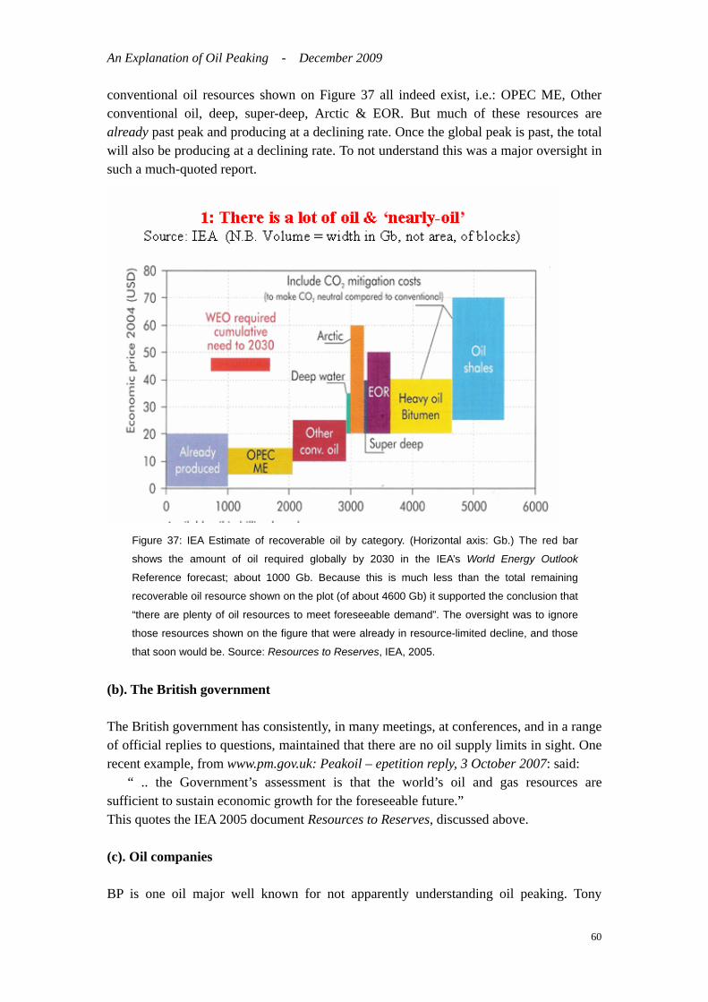
An Explanation of Oil Peaking - December 2009
conventional oil resources shown on Figure 37 all indeed exist, i.e.: OPEC ME, Other conventional oil, deep, super-deep, Arctic & EOR. But much of these resources are already past peak and producing at a declining rate. Once the global peak is past, the total will also be producing at a declining rate. To not understand this was a major oversight in such a much-quoted report.
Figure 37: IEA Estimate of recoverable oil by category. (Horizontal axis: Gb.) The red bar
shows the amount of oil required globally by 2030 in the IEA’s World Energy Outlook
Reference forecast; about 1000 Gb. Because this is much less than the total remaining
recoverable oil resource shown on the plot (of about 4600 Gb) it supported the conclusion that
“there are plenty of oil resources to meet foreseeable demand”. The oversight was to ignore
those resources shown on the figure that were already in resource-limited decline, and those
that soon would be. Source: Resources to Reserves, IEA, 2005.
(b). The British government The British government has consistently, in many meetings, at conferences, and in a range of official replies to questions, maintained that there are no oil supply limits in sight. One recent example, from www.pm.gov.uk: Peakoil – epetition reply, 3 October 2007: said: “ .. the Government’s assessment is that the world’s oil and gas resources are sufficient to sustain economic growth for the foreseeable future.” This quotes the IEA 2005 document Resources to Reserves, discussed above. (c). Oil companies BP is one oil major well known for not apparently understanding oil peaking. Tony
60

An Explanation of Oil Peaking - December 2009
Hayward, CEO of BP, said in June 2008: “Myth number two is that the world is running out of hydrocarbons. Not so. The world has ample resources, with more than 40 years of proven oil reserves …”. Peter Davies, former Chief Economist at BP, has been more explicit. At a meeting of the All-Party Parliamentary Group on Peak Oil in the House of Commons he maintained that any peak has to be far off because “the World has 40 years’ of proven reserves.” ExxonMobil, as another example, ran a notable advertising campaign recently under the banner: “The [oil] peak is not in sight.” And ENI’s Chief Economist, Leonardo Maugeri, has published widely dismissing the idea of a near- or medium-term oil peak. (d). Academic institutions, & Authors Examples include recent papers by Aguilera et al. of the Colorado School of Mines estimating the size of the global recoverable oil base. These papers point to the latter’s large size, and hence the authors discount the probability of a near- or medium-term oil peak. (This view from the School of Mines is unfortunate. The School’s L. Ivanhoe understood the oil peak. He questioned early on the analysis of B. Grossling of the USGS suggesting that many world regions must contain much undiscovered oil because they had not been drilled to the same extent as the US. He gave a knowledgeable commentary in the Open University film mentioned above. More recently he published an excellent paper in the Oil & Gas Journal on future global oil supply based on a solid understanding of peaking,) G. Campbell Watkins, for many years a well-known UK authority on oil supply, dismissed any risk of near term supply peaking. His view was informed by the apparently solid evidence of the ever-increasing volume over many years of the world’s proven oil reserves (see Figure 38, below). (G. C. Watkins. Oil scarcity: what have the past three decades revealed? Energy Policy 34, 508-514, 2006.) A third example in this category is the recent book by Robin Mills: The Myth of the Oil Crisis; Praeger, 2008. The majority of statements in this book are quite correct; along the lines of: ‘There is more oil to be found in region X’, and ‘Technology has increased the recovery factor of field Y’. However, at least apparently, Mills did not feel the need to discuss the topic of oil peaking with anyone who understands it. Sadly, this criticism applies to many who comment on the topic. (Indeed, this it one of the aspects of oil depletion that your present author does not fully understand: why - to this author’s knowledge - not one of those who have criticised oil peak analysis has asked to see the data. This is probably partly explained next.) Some explanations of why these authorities did not understand oil peaking It is probable that the primary reasons why the above authorities and others have not understood the oil peak are:
61

An Explanation of Oil Peaking - December 2009
- Since the late 1980s there have been very few analysts working quantitatively in the area. - In recent years there have been few readily-available explanations of peaking. (This paper is intended, in part, to help rectify this.) - There has been a strong ‘economic’ counter-theory to peaking that has been widely held, including within the oil industry. This theory is set out in the Annex. - Finally, a great confusion has existed over the difference between 1P and 2P reserves, and particularly over the significance of their evolution with time, as indicated in Figure 38.
World remaining oil reserves from political and technical sources
0
200
400
600
800
1000
1200
1400
1940 1950 1960 1970 1980 1990 2000 2010
year
technical = 2P = proven+probable =backdated mean excluding extra-heavy oilpolitical = 1P = current so called proved
Jean Laherrere 2008
omission of probableincorrect aggregation
OPEC fight for quotas +300 Gb = speculative resources al-Husseini (Aramco)
including tarsands +175 Gb
Ghawar
Sources: IHS, USDOE, CAPP, OGJ
Figure 38: Evolution of Global Oil Reserves: “Reality vs. Illusion”. (Ordinate: Gb.)
- The Figure shows (green line) the change over time of global backdated ‘proved plus
probable’ (2P) oil reserves, excluding extra-heavy oil and tar sands. This indicates that 2P
discovery was well ahead of production from the 1950s to 1970s, but has fallen below
production since 1980.
- The magenta line shows the evolution of global proved (1P) reserves since 1950. These
would seem to indicate, by contrast, that ‘discovery’ has kept ahead of production over the
whole of this period, with the “world running into oil” in Odell’s phrase, not out of it. The jump in
the late 1980s was due to the OPEC ‘quota wars’ proved reserves increases; the more recent
increase is due to the inclusion of tar sands reserves.
Source: Laherrère; with original data sources as indicated. 7. Conclusions The conclusions to be drawn from the above are as follows:
62
An Explanation of Oil Peaking - December 2009
7.1 What is Oil Peaking? This paper has shown that there is much misunderstanding about what is oil peaking. The term ‘oil peak’, as used here, refers to the production of conventional oil (not, for example, to tar sands or oil shales); to oil in a region (not from a single field; this too peaks, but often not near the mid-point of the field’s recoverable resource); and to the point when maximum production is constrained by the quantity of the recoverable resource (and not set, e.g., by government or company dictat). The peak usually occurs when about half or less of the total recoverable resource in the region has been produced. 7.2 The Mechanism of the Oil Peak The mechanism of the oil peak for conventional oil production is quite simple. It occurs when the discovery of new fields in a region has been in decline for some time, such that declining production from the generally larger early fields can no longer be offset by production from the numerous, but generally smaller and harder to find, later fields. The main driver behind this dynamic is the skewed distribution of oil in fields, such that most of the oil lies in relatively few fields. Because these large fields are generally easier to discover, they usually get into production first. - The typical shape of the production curve in many regions before and after peak is now well-established. Production usually rises in a ‘bell-like’ curve towards peak, and declines with a long tail afterwards. (The symmetric bell-shape shape of the logistic curve is mathematically convenient for predicting peak, but is usually a fairly poor model of production post-peak.) - The shape of the proved plus probable (‘2P’) cumulative discovery curve is also not usually logistic. It is usually more akin to parabolic; going up steeply as the initial large fields are found, and flattening out towards an asymptote as the discovery rate declines. Many regions have succeeding phases of discovery, putting ‘steps’ in the discovery curve. These ‘steps’ are often - but by no means always - smaller than the preceding ones. 7.3 The Peak is Counter-intuitive The resource-limited production peak is strongly counter-intuitive. It cannot be foreseen by looking at current production and reserves data, and typically occurs when: - production in a region has been trending steadily upward; - the region still has very significant reserves; - discovery of new fields is continuing; - technology is raising recovery factors in fields already discovered. 7.4 Forecasting peak To visualise the likelihood of a region peaking, it is helpful to plot 2P discovery and production on a single plot vs. time (with sometimes the discovery data needing
63

An Explanation of Oil Peaking - December 2009
averaging, over say a five-year period, to fit easily to the same scale). Judgement by eye can then say how much of the discovered has been produced; with the peak expected when roughly half - or a bit less - has been produced. However, a 2P discovery trend by itself cannot predict the URR in a region; it must be combined with geological knowledge of what extra recoverable resources the region is likely to yield. For an indication that a declining discovery trend is a reliable estimate of a region’s URR, and that there is not a large volume of oil still to be discovered - a useful plot is that of cumulative 2P discovery and production versus time. On this plot independent estimates, if available, of URR for the region can be shown against a future date. The production peak might then be expected when cumulative production reaches perhaps 35% to 55% of the ‘discovery-trend’ URR; and perhaps 20% to 35% of a higher URR (for example, one that contains large estimates for reserves growth). This report has given examples of such plots. There are many methods for predicting the future date of the resource-limited peak in a region. These include looking at past discovery, at yield-per-effort; at simple mid-point peaking (where the URR derives from the discovery trend); and at detailed bottom-up by-field models. See the Global Oil Depletion report from UKERC, at www.ukerc.ac.uk, for details of current forecasting techniques. On the other hand, there are many ways not to forecast oil production: - Never use proved reserves (‘1P’) for assessing the scope for future oil production. These data are usually under-reported, are sometimes over-reported, and are consistently not-reported. - Neither rely on an R/P ratio to indicate security of supply. Not only are the 1P data poor, but the R/P ratio ignores the fundamental oil peaking mechanism. For example, the global production of conventional oil will peak when the world’s R/P ratio will be close to its current value of 40 years’ of supply. - Be cautious of ‘quasi-linear’ models that calculate future demand and then assign recoverable resources to meet this. Often such models ignore the mechanism of peaking, as well as empirical limits on discovery rate, and on depletion rate (where the latter is production divided by remaining recoverable resources). 7.5 Economic Issues Economic arguments and other ‘above-ground’ factors should be included in the models. But it would be wrong to expect a higher oil price - or advancing technology - to significantly shift the expected date of the production peak in a region once 2P discovery has been in decline for an extended period. Thus the peaks illustrated in this paper are resource-limited, in that they reflect a lack of
64

An Explanation of Oil Peaking - December 2009
recoverable oil in the fields in a region, and not simply a lack of investment. While extraordinarily high levels of investment could, in some of these regions, still push production above the former ‘peak’ levels for a short while (for example, by very extensive and rapid in-fill drilling of existing fields, and by a crash programme of exploration drilling), such investments would make little economic sense, and production would fall very rapidly thereafter. 7.6 Uncertainties Current uncertainties include: - The true size of most Middle East countries’ 2P reserves. - Reliable 2P ‘reserves growth’ data for most regions. - The impact of reserves growth on dates of peak. (But as the examples above, such as the UK and the US, indicate, even quite significant reserves growth in a region appears to do little to delay the date of the region’s resource-limited production peak.) - The ‘above-ground’ factor of the willingness of the large producers to pump as fast as high levels of investment might permit. 7.7 Production of non-conventional oil, and ‘all-liquids’ For the non-conventional oils, the potential resources are very large, and for almost all, their locations are known so exploration costs are low. However, for these oils there are a range of constraints that are likely to limit production. These include: - technological readiness; - a high investment requirement, typically, per barrel pumped; - resource requirements (energy, water, land for waste); - CO2 emissions; - net-energy related cost and energy-yield factors;
- net-energy rate limits, reflecting the fact if any new energy-saving, or energy-producing, technology is introduced faster than the energy embodied in new plant, the overall net-energy yield is negative during the growth phase.
7.8 Summarising
• Conventional oil peaking is reasonably well understood. The production peak in region occurs when typically something less than half the region’s ultimately recoverable reserves (URR) have been produced; and often closer to one-quarter of the URR if the latter includes a significant allowance for reserves growth.
• Production forecasts that rely on a large URR for a region, or on an R/P ratio of many years, to assert that “there is plenty of oil to meet foreseeable demand” will be incorrect if they do not also take into account the mechanism of the production peak.
• The date of the peak for conventional oil can be calculated with reasonable precision by a range of models. For the world, this date is close - almost certainly before 2020.
65

An Explanation of Oil Peaking - December 2009
• The main technical unknowns in the models are the size of Middle East 2P reserves, and the likely impact on peak of reserves growth in existing fields.
• The main ‘above-ground’ unknown is the willingness of the large producers to invest in increased production.
• Once conventional oil production has peaked, if the historic growth of global demand is to be met, the quantity of oil required from non-conventional sources grows rapidly. For example, to meet ‘business-as-usual’ demand 10 years after the global conventional oil peak, a production of up to 30 Mb/d will have to be produced from these other sources. It is not clear that these ‘other oils’ can be produced fast enough in sufficient quantities, especially if limits on CO2 emissions are taken into consideration.
----------------------------------------------- END ----------------------------------------------- Annex: Some ‘Economic Views’ of Oil Depletion A number of influential energy economists have espoused the following ideas, to varying degrees, to argue against the notion of oil peaking. Discussion of the validity most of these ideas has been given in the main article above; additional notes are given below. 1. The cost of any mineral reflects a race between depletion of its resource and
mankind’s increasing technological skill at extraction. To-date, for no significant mineral has this race been lost, and empirical data indicate that the long-term extraction cost of nearly all minerals has always fallen. There is no reason to expect oil to be an exception.
2. The price of oil indicates future supply. Currently neither price nor more detailed economic metrics indicate approaching supply difficulties. These indicators will give sufficient warning should such difficulties approach. (a)
3. Markets function very well. Were an oil shortage to be imminent, the increasing price of oil would increase exploration, exploitation of currently uneconomic fields, recovery factors, use of alternative oils, and substitution away from oil. These changes, in combination with a fall in demand also driven by price, would bring the market back into balance. In essence, oil (and energy also) is simply a commodity; supply is best left to the market. (b)
4. For most countries, the cost of oil is only a small percentage of GDP; even a substantial rise in oil price will have only a modest impact on their economies.
5. There are over 40 years’ of proved oil reserves. This is secure, known oil extractable at to-day’s prices. More oil will also be found. Any potential oil supply problem must be many decades into the future.
6. There are still plenty of places to look for oil. Large oil discoveries have been made in the Caspian, deep offshore, etc., and there are still many promising oil basins that have seen little exploration.
7. Moreover, the bulk of ‘new oil’ comes not from discovery, but from revisions and extensions to existing fields. Such ‘reserves growth’ will be a key contributor to future supply.
66

An Explanation of Oil Peaking - December 2009
8. Indeed, oil reserves are merely ‘inventory’. Oil companies keep a given number of years’ supply on their books, and as supply falters more of the effectively infinite oil resource base gets turned into reserves. The data confirm this has always happened in the past.
9. There exist vast resources of non-conventional oil. These include 300 billion barrels of recoverable oil each in the Orinoco basin and Athabasca, with the total in-place oil resource at these sites amounting to several trillions of barrels. There is an even larger amount of oil in shale deposits around the world. This distribution is expressed by a ‘resource pyramid’, with a small volume of low-cost oil at the top, and an ever-increasing volume of more expensive, or otherwise less desirable oil, further down the pyramid. (c)
10. Should the supply of oil itself ever become difficult, it can be substituted by gas, of which there are large stranded supplies; by gas-to-liquids, biofuels and other oil substitutes; and, if the need arises, by coal. Large volumes of gas hydrates may also prove economically extractable.
11. Virtually none of the bodies one would expect to warn of impending supply shortages are currently predicting any risk to supply. These include oil companies and consultancies, as well as authorities such as the IEA, the US’ EIA or the USGS.
In addition to the above general views, some economists have offered the following specific criticisms of the geologists’ calculations: 12. Geologists rely on industry data that are not in the public domain. Analysts cannot
check that these data are correct, nor that the geologists are interpreting them correctly.
13. The geologists ignore the effects of price and technology gain. Without such obvious feedbacks, simple geology-based modelling is without validity.
14. Past oil forecasts have all been wrong. Thirty years ago it was believed that oil would run out in thirty years, to-day the world has forty years’ worth of reserves. It is foolish of the geologists to forecast oil’s future on the basis of an assumed fixed volume of oil.
15. The ‘Hubbert curve’, used by some geologists in their modelling, is a poor match to actual production, especially well past peak.
16. The geologists who forecast a near-term oil production decline have shown a steady upward revision in the resource volumes they assume.
Taken together, the above is an impressive list. It appears to give almost incontrovertible evidence that no near-term oil supply problems lie ahead. Instead - as has been shown in the main body of this paper - the majority of these arguments do not stand up to detailed examination, and where true in part they need quantification if they are to usefully contribute to forecasting oil’s future. Notes
(a). The lack of a price signal for oil peaking has been widely quoted, at least up to
67

An Explanation of Oil Peaking - December 2009
about mid-2004. What the economists say in the face of the recent price rises is not yet fully clear, though Chinese demand and lack of refinery capacity are mentioned. In terms of understanding the price signal it is useful to recognise that it is very difficult for the price to reflect other than the near term supply/demand balance. This is because when selling any widely-traded commodity it is hard for sellers to hold out when prices fall, even if it is only in the short term. Note however that sequestration of Middle East assets from the commercial oil companies by the nationals, followed by OPEC quotas, meant that higher cost oil (North Sea, Alaska, and now deep offshore) has been produced while lower cost Middle East oil has remained in the ground. Had the ‘seven sisters’ remained in control it is likely that a steady oil price rise would have taken place as the cheap oil depleted first. Incidentally, that there was a price signal before 1970s oil shocks but this was small and ignored. (b). See comments on Lord Lawson’s views of ‘energy as a commodity’ in: Bentley, R.W., et al. The Oil Future - A Very Different View, Newsletter of the Int'l. Assocn. for Energy Economics, 4th Quarter, 1999. (c). In terms of the ‘resource pyramid’ concept, oil is not like a conventional mineral with an infinite continuum of lower concentration ores. For conventional oil there is a well-defined water boundary in most reservoirs below which there is no oil: oil comes in packets. So the ‘lower concentration ores’ are simply the smaller fields, and here it is easy to extrapolate both field size and discovery rate to calculate how much will be found with any specified discovery effort. Additionally, oil is not a mineral such as gold or aluminium which if really needed can be extracted at high cost; oil is not worth extracting if this requires more energy than it yields. These special aspects of oil require economists to be cautious when applying general resource theories. Notes & References (To avoid breaking the flow above, the following approach to referencing has been adopted.) IEA recently estimated …. at nearly 10 trillion barrels. IEA World Energy Outlook 2007 page 42. (And see Figure 37) Over 85% of all oil produced to-day is conventional oil.
and CO NGLs, tertiary/EOR (steam drive, N2 2; and non-conventional (primarily tar sands); plus an increasing amount of biofuels, mostly in the US & Brazil. Figure1a: A simplified model of why production In this simple model, the life of fields is unrealistically short, and the rate of starting new fields – 1 per year – rigid and too slow. But if you play around with more realistic values (large fields with a 40 to 120 year life; smaller ones with 10 to 30 year life); time to plateau or peak – typically 2 to 10 years; again in part depending on field size; and with rates on-steam, always graphs at least along the general lines of Figure 1a result. The
68

An Explanation of Oil Peaking - December 2009
slightly unrealistic parameters for Figure 1a have been chosen to make the mechanism of peak easy to see. Here each triangle represents the production from a single field. As can be seen, production from each field starts in succeeding years; and each succeeding field is smaller than the preceding one; in this case, 90% of the size See data from DECC (formerly DTI; & earlier: UK Dept. of Energy). From these three simple assumptions some surprising properties emerge: See modelling by London University, QMC of ‘adding triangles’. … which [Hubbert] later depicted on film. Film by the UK’s Open University. Many sizeable regions of the world are now past their conventional oil resource-limited peak - over 60 countries, Data from Energyfiles, UK. ‘ … production trend at that date, and forecast production increases for many years to come. Peter Davies, Michael Lynch, John Mitchell, others. The decline is often modelled as exponential. Where the oil drive is purely by expansion of a gas cap, such a fall-off has a theoretical basis. ‘Perfect’ water drive, by contrast, would result in constant production until the oil is exhausted. Real fields, however, generally contain faults and inhomogeneities which play havoc with such theoretical profiles. Most fields, moreover, see additional investment that changes the profile otherwise expected. Nevertheless, the norm for nearly all fields is for a long production decline once plateau or peak is past; see examples in the cumulative plots of production by field.
Figure 39: Simplified model of production in a region. If fields exhibit trapezoidal-shaped
production the peak is clear, but sharper and later.
69
An Explanation of Oil Peaking - December 2009
… the smaller fields generally come on-stream later. There have been many studies of field size distribution in basins, but here we also need to deal with in what order these fields are discovered; and more specifically, in what order they are brought into production. Moreover, since we are often modelling regions such as countries; these may contain several basins. It is generally true, however - and see the examples earlier - that the larger fields in a region are easiest to find, and hence get found first; while the economics of production helps ensure that large finds will generally get into production before smaller ones. So here also the model seems to capture reality. UK Ultimates … This is not to ignore the impact of price. The UK’s large early offshore fields were discovered before the 1973 price shock, by which point the discovery trend had set in, and credible estimates of ultimate had become possible. But the speed of exploiting these finds, and hence production, would almost certainly have been less had the oil price remained low. For any given region the 2P discovery says what has been found, and the 2P creaming curve says what is likely to be found. Production profiles then set out the maximum likely rate that these fields can be produced. This information gives the resource-limited production rate for the region. It does not say that this production will actually be obtained, as politics, a low price, or other factors can always slow production. Most analysts then – and still today – treat proved reserves as a fairly accurate measure of the amount of oil likely to be available. E.g., Stevens & Mitchell, recent report for Chatham House, UK. The replacement of the proved reserves was thus very widely ascribed, including within the IEA, as being due to improvements in technology; horizontal drilling and 4-D seismic being frequently cited. In an IEA WEO – probably 2006. 1998 or 1999. Given the general straightness of the cumulative production line, despite the trough from 1985 to 1995, this date can be predicted with reasonable precision from the first years of production. Readers may wish to put symmetric triangles on the production data for full range of ultimates & see how insensitive is the date of peak … that by L. Maugeri, the Chief Economist of ENI, in Science. See: Maugeri L. Oil: never cry wolf — Why the petroleum age is far from over. Science 2004; 304:1114–5; and also: Q.Y. Meng and R.W. Bentley. Response to L. Maugeri: Why the world should not count on abundant supplies of oil. Energy, vol. 8, pp 1179-1184, 2008. The models we examined within a recent UKERC study … S.R. Sorrell et al. Global Oil Depletion – An assessment of the evidence for a near-term peak in global oil production. A Technology Policy Assessment study for the
70
An Explanation of Oil Peaking - December 2009
UK Energy Research Centre, August 2009. ISBN: 1-903144-0-35. Available from www.ukerc.ac.uk. Acknowledgements Useful conversations – sometimes many – have been held with the following: Colin Campbell, Jean Laherrère, George Leckie, Ken Chew, Francis Harper, Richard Miller, Chris Skrebowski, Michael Smith, David Strahan, Richard Hardman, Jeremy Leggett, Peter Jackson, Steve Sorrel, Jamie Speirs; Pierre-René Bauquis, Jean Marie Bourdaire, Fatih Birol, Peter Gerling, Klaus Illum, Kjell Aleklett, Mikael Höök, Rui Rosa, Ugo Bardi, Jörg Schindler, Werner Zittel; L. Ivanhoe, Tom Alhbrandt, Gregory Ulmeshek, Ron Charpentier, Robert Hirsch, Mike Rodgers, David Greene, Ken Deffeyes and Hilary Smith. Apologies to those omitted from this list. In addition, I have much appreciated conversations with the following, though often disagreeing with the views expressed: Georges DuPont-Roc, Peter Davies, David Frowd, Hans Maters, Peter Odell, Alex Kemp, Paul Stevens, John Chesshire, John Mitchell, Robert Mabro, M. Adelman, Michael Lynch. Colin Campbell and Jean Laherrère kindly reviewed an earlier draft of this paper. The membership of the University of Reading, UK, ad hoc ‘Oil Resources Group’, past and present, has been: Postgraduate Research Institute for Sedimentology: Prof. M.L. Coleman (ex-BP), Prof. B.W. Sellwood. Department of Engineering: Dr. J.D. Burton, Mr. R.H. Booth (ex-Shell), Dr. R.M. Mayer (ex-BP), Prof. P.D. Dunn; MSc. Students: L. Kurdgelashvili, S. Mannan. Department of Cybernetics: Dr. G.R. Whitfield, Dr. R.W. Bentley (ex-Exxon). Affiliated: Dr. D. Fleming, independent economist. Also Students: S. Olayiwola, City University; Q. Meng, CUP, Beijing, China. For many years the above was the only academic group in the UK carrying out quantitative research on the future of global hydrocarbon supply. Publications from members of the group have included: R.W. Bentley. The Expected Dates of Resource-limited Maxima in the Global Production
of Oil and Gas. Accepted for publication: Springer. S. Sorrell, J. Speirs, R. Bentley, A. Brandt, R. Miller. Global Oil Depletion - An
assessment of the evidence for a near-term peak in global oil production. Report: UK Energy Research Centre, August 2009.
71

An Explanation of Oil Peaking - December 2009
Q.Y. Meng and R.W. Bentley. Response to L. Maugeri: Why the world should not count on abundant supplies of oil. Energy, vol. 8, pp 1179-1184, 2008.
R.W. Bentley and G.A. Boyle. Global oil production: forecasts and methodologies. Environment and Planning B: Planning and Design, vol. 35, pp 609-626, 2008.
R.W. Bentley, S.A. Mannan, and S.J. Wheeler. Assessing the date of the global oil peak: The need to use 2P reserves. Energy Policy, vol. 35, pp 6364–6382, Elsevier, 2007.
R.W. Bentley and M.R. Smith. World Oil Production Peak - A Supply-Side Perspective. Int’l. Assocn. for Energy Economics Conference, Prague, June 2003.
R.W. Bentley. Oil Forecasts, Past and Present. Energy Exploration and Exploitation, Vol. 20, No. 6, pp 481-492, Multi-Science Publishing Co. Ltd., 2002.
R.W. Bentley. Global oil and gas depletion: an overview. Energy Policy, Vol. 30, No. 3, February 2002, pp 189-205. Elsevier, 2002.
R.W. Bentley, R.H. Booth, J.D. Burton, M.L. Coleman, B.W. Sellwood, G.R. Whitfield. World Oil Supply: Near & Medium-Term. Report submitted to the DTI's Energy Advisory Panel, Sept 5th, 2000.
R.W. Bentley, R.H. Booth, J.D. Burton, M.L. Coleman, B.W. Sellwood, G.R. Whitfield. Perspectives on the Future of Oil. Energy Exploration and Exploitation, Vol. 18, Nos. 2 & 3, pp 147-206, Multi-Science Publishing Co. Ltd., 2000.
R.W. Bentley, R.H. Booth, J.D. Burton, B.W. Sellwood, G.R. Whitfield. The Oil Future - A Very Different View. Newsletter, Int'l. Assocn. for Energy Economics, 4th Quarter, 1999.
72