annex a : design drivers 1 the indian rural scenariosri/projects/wifire/wifire-annex-lines.pdf ·...

WiFiRe Specifications, Aug 2006 draft

ANNEX A : Design Drivers1

1 The Indian Rural Scenario2

About 70% of India’s population, or 750 million, live in its 600,000 villages. More than 85%3

of these villages are in the plains or on the Deccan plateau. The average village has 200-2504

households, and occupies an area of 5 sq. km. Most of this is farmland, and it is typical to find5

all the houses in one or two clusters. Villages are thus spaced 2-3 km apart, and spread out in all6

directions from the market towns. The market centers are typically spaced 30-40 km apart. Each7

such centre serves a catchment of around 250-300 villages ina radius of about 20 km. As the8

population and the economy grow, several large villages arecontinually morphing into towns and9

market centres.10

The telecommunication backbone network, mostly optical-fiber based, which passes through these11

towns and market centers, is new and of high quality. The state-owned telecom company has12

networked exchanges in all these towns and several large villages with optical fiber that is rarely13

more than 10-15 years old. The mobile revolution of the last four years has seen base stations14

sprouting in all these towns, with three or more operators, including the state-owned company.15

These base stations are also networked using mostly opticalfiber laid in the last 5 years. There is16

a lot of dark fiber, and seemingly unlimited scope for bandwidth expansion.17

The solid telecom backbone that knits the country together ends abruptly when it reaches the towns18

and larger villages. Beyond that, cellular coverage extends mobile telephone connectivity up to a19

radius of 5 km, and then telecommunications simply peters out. Cellular telephony will expand20

further as it becomes affordable to the rural populace. It isa highly sought after service, and the21

only reason for the service not spreading as rapidly in ruralareas as in urban areas is the lack of22

purchasing power in the the rural areas. Fixed wireless telephones have been provided in tens of23

thousands of villages as a service obligation; however, thewireless technologies currently being24

deployed can barely support dial-up speeds as far as Internet access is concerned.25

The rural per capita income is distinctly lower than the national average, and rural income distri-26

bution is also more skewed. About 70% of the rural householdsearn less than Rs 3000 per month,27

and only 4% have incomes in excess of Rs 25000 per month. Only the latter can be expected to28

even aspire to have a personal computer and Internet connection. For the rest, the key to Internet29

access is a public kiosk providing a basket of services. Provision of basic telecommunications as30

well as broadband Internet services is imperative, since ICT is known to be an enabler for wealth31

creation32

2 Affordability33

When considering any technology for rural India, it is clearthat the question of affordability must34

be addressed first. Given the income levels, one must work backwards to determine the cost of any35

economically sustainable solution. It is reasonable to expect an expenditure on telecommunication36

75 Copyright c©2006 CEWiT, Some rights reserved


services of only around Rs 60 per month on the average (2% of household income) from about1

70% of the 200-250 households in a typical village. Thus, therevenue of a public kiosk can only2

be of the order of Rs 4500 per month (assuming two kiosks per village on the average). Apart from3

this, a few wealthy households in each village can afford private connections. Taking into account4

the cost of the personal computer, power back-up, peripherals, etc, it is estimated that a cost of5

at most Rs 15000 per broadband connection is sustainable forthe kiosk. This includes the User6

Equipment, as well the per-subscriber cost of the Network Equipment connecting the user to the7

optical fiber PoP.8

A typical wireless system for servicing such a rural area will have a BTS at the fiber PoP. A BTS9

can be expected to serve about 250-300 connections initially, going upto a 1000 connections as10

the service becomes stable and popular and the wealthy households decide to invest in a computer.11

Growth to full potential will take several years. Given the cost target mentioned above, it is found12

that a wireless technology becomes economically viable in the rural areas only when it has reached13

maturity and volumes worldwide are high enough to bring the cost down. New technologies at the14

early induction stage are too costly, particularly since the slow growth in the subscriber base keeps15

the per-subscriber cost of the BTS and associated equipmenthigh.16

3 Coverage, Towers and System Cost17

We have already mentioned that we need to cover a radius of 15-25 km from the PoP using wireless18

technology. The system gain is a measure of the link budget available for overcoming propagation19

and penetration losses (through foliage and buildings) while still guaranteeing system performance.20

Mobile cellular telephone systems have a system gain typically of around 150-160 dB, and achieve21

indoor penetration within a radius of about 3-5 km. They do this with Base Station towers of 4022

m height, which cost about Rs 5 lakhs each. If a roof-top antenna is mounted at the subscriber23

end at a height of 6m from the ground, coverage can be extend upto 15-20 km with this system24

gain. When the system gain is lower at around 135 dB, as with many low-power systems such25

as those based on the WiFi standard or the DECT standard [19],coverage is limited to around 1026

km and antenna-height at the subscriber-end has to be at least 10m. This increases the cost of the27

installation by about Rs 1000.28

In any case, we see that fixed terminals with roof-top antennas are a must if one is to obtain the29

required coverage from the fiber PoP. A broadband wireless system will need a system gain of30

around 140 - 150 dB at bit-rates in excess of 256 kbps, if it is to be easily deployable. This system31

gain may be difficult to provide for the higher bit-rates supported by the technology, and one may32

have to employ taller poles in order to minimize foliage loss.33

There is an important relationship between coverage and theheights of the towers and poles, and34

indirectly their cost. The Base Station tower must usually be at least 40 m high for line-of-sight35

deployment, as trees have a height of 10-12m and one can expect a terrain variation of around36

20-25m even in the plains over a 15-20 km radius. Taller Base Station towers will help, but the37

cost goes up exponentially with height. A shorter tower willmean that the subscriber-end will38

need a 20 m mast. At Rs 15000 or more, this is substantially costlier than a pole, even if the mast39



is a guyed one and not self-standing. The cost of 250-300 suchmasts is very high compared to1

the additional cost of a 40 m tower vis--vis a 30 m one. With the40m towers, simple poles can be2

deployed at the subscriber-end, and these need be only than 12m high.3

In summary, one can conclude that for a cost-effective solution the system gain should be of the or-4

der of 145 dB, (at least for the reasonable bit-rates, if not the highest ones supported), a 40 m tower5

should be deployed at the fiber PoP, and roof-top antennas with 6-12m poles at the subscriber-end.6

The system gain can be lower at around 130 dB, provided repeaters are used to cover areas be-7

yond 10 km radial distance, and assuming antenna poles that are 10-12m high are deployed in the8

villages. The cost per subscriber of the tower and pole (assuming a modest 300 subscribers per9

tower) is Rs 2500. This leaves about Rs 12500 per subscriber for the wireless system itself.10

4 Definition of Broadband11

The Telecom Regulatory Authority of India has defined broadband services as those provided12

with a minimum downstream (towards subscriber) data rate of256 kbps. This data-rate must13

be available unshared to the user when he/she needs it. At this bit-rate, browsing is fast, video-14

conferencing can be supported, and applications such as telemedicine and distance education using15

multi-media are feasible. There is no doubt that a village kiosk could easily utilise a much higher16

bit-rate, and as technology evolves, this will become available too. However, it is important to note17

that even at 256 kbps, since kiosks can be expected to have a sustained rate not much lower, 30018

kiosks will generate of the order of 75 Mbps traffic to evacuate over the air per Base Station. This19

is non-trivial today even with a spectrum allocation of 20 MHz.20

The broadband wireless access system employed to provide Internet service to kiosks must also21

provide telephony using VoIP technology. Telephony earns far higher revenue per bit than any22

other service, and is an important service. The level of teletraffic is limited by the income levels of23

the populace. Assuming that most of the calls will be local, charged at around Rs 0.25 per minute,24

even if only one call is being made continuously from each kiosk during the busy hours (8 hours per25

day), this amounts to an expenditure of Rs 120 per day at each kiosk. This is a significant fraction26

of the earnings of the kiosk, and a significant fraction of thetotal communications expenditure of27

the village.28

Thus, depending on the teledensity in the district, one can expect around 0.5-1 Erlang traffic per29

kiosk. This works out to a total of around 100-200 Erlangs traffic per BTS. Assuming one voice call30

needs about 2x16 kbps with VoIP technology, this traffic level requires 2x1.5 Mbps to 2x3.0 Mbps31

of capacity. If broadband services are not to be significantly affected, the system capacity must be32

several times this number. It is to be noted here that if the voice service either requires a higher33

bit-rate (say, 64 kbps) per call, or wastes system capacity due to MAC inefficiency when handling34

short but periodic VoIP packets, we will have significant degradation of other broadband services.35

Thus, an efficient VoIP capability is needed, with QoS guaranteed, that eats away from system36

capacity only as much as is unavoidably needed to support thevoice traffic. Such a capability must37

be built into the wireless system by design. It is also important not to discourage use of the system38

for telephony since it is the major revenue earner as well as most popular service.39



5 Broadband Wireless Technologies circa 20061

One of the pre-requisites for any technology for it to cost under Rs 12500 per connection is that2

it must be a mass-market solution. This will ensure that the cost of the electronics is driven down3

by volumes and competition to the lowest possible levels. Asan example, both GSM and CDMA4

mobile telephone technologies can today meet easily meetthe above cost target, except that they5

do not provide broadband access.6

The third-generation evolution of cellular telephone technologies may, in due course, meet the cost7

target while offering higher bit-rate data services. However, they are ain the early induction stage8

at present, and it is also not clear whether they will right away provide the requires system capacity.9

However, the third-generation standards are constantly evolving, and the required system capacity10

is likely to be reached at some time. The only question is regarding when the required performance11

level will be reached and when the cost will drop to the required levels.12

If we turn our attention next to some proprietary broadband technologies such as iBurst [7], and13

Flash-OFDM [8], or a standard technology such as WiMAX-d (IEEE 802.16d) [10], we find that14

volumes are low and costs high. Of these, WiMAX-d has a lower system gain. All of them will15

give a spectral efficiency of around 4 bps/Hz/cell (after taking spectrum re-use into account), and16

thus can potentially evacuate 80 Mbps with a 20 MHz allocation. High cost is the inhibitory factor.17

It is likely that one or more OFDMA-based broadband technologies will become widely accepted18

standards in the near future. WiMAX-e (IEEE 802.16e) [10] isone such that is emerging rapidly.19

The standards emerging as the Long-Term Evolution (LTE) of the 3G standards are other can-20

didates. These will certainly have a higher spectral efficiency, and more importantly, when they21

become popular and successful, they will become mass-market technologies, and the cost will be22

low. Going by the time-to-maturity of mass-market wirelesstechnologies till date, none of these23

technologies are likely to provide an economically viable solution for India’s rural requirements24

for several years yet.25

6 Alternative Broadband Wireless Technologies in the Near Term26

While wide-area broadband wireless technologies will be unavailable at the desired price-performance27

point for some time, local-area broadband technologies have become very inexpensive. A well-28

known example is WiFi (IEEE 802l.11) technology. These technologies can provide 256 kbps or29

more to tens of subscribers simultaneously, but can normally do so only over a short distance, less30

than 50m in a built-up environment. Several groups have worked with the low-cost electronics31

of these technologies in new system designs that provide workable solutions for rural broadband32

connectivity.33

One of the earliest and most widely deployed examples of suchre-engineering is the corDECT34

Wireless Access System [9] developed in India. A next–generation broadband corDECT system35

has also been launched recently, capable of evacuating upto70 Mbps per cell in 5 MHz bandwidth36

(supporting 144 full-duplex 256 kbps connections simultaneously). These systems are built around37



the electronics of the European DECT standard, which was designed for local area telephony and1

data services. Proprietary extensions to the DECT standardhave been added in a manner that the2

low-cost mass-market ICs can continue to be used. These increase the bit-rate by three times, while3

being backward compatible to the DECT standard.4

The system gain in Broadband corDECT for 256 kbps service is 125-130 dB, depending on the5

antenna gain at the subscriber-end. This is sufficient for 10km coverage under line-sight conditions6

(40 m tower for BS and 10-12 m pole at subscriber side). A repeater is used for extending the7

coverage to 25 km. The system meets the price-performance requirement, but with the additional8

encumbrance of taller poles and one level of repeaters.9

The WiFiRe standard proposed by CEWiT is an alternative near-term solution, with many simi-10

larities. It, too, is a re-engineered system based on low-cost low-power mass-market technology.11

Cost structures are similar, and deployment issues too are alike. There is one key aspect in which12

WiFiRe differs from Broadband corDECT. The spectrum used for WiFiRe is unlicensed without13

fees, whereas the spectrum used by Broadband corDECT is licensed with a fee. The spectral ef-14

ficiency of the WiFiRe system is poorer, and the cell capacityper MHz of bandwidth is lower.15

However, this is offset by the fact that the spectrum used by it is in the unlicensed WiFi band of16

2.4-2.485 MHz. This unlicensed use is subject to certain conditions, and some modifications to17

these conditions will be needed to support WiFiRe in rural areas (see section on Conditional Li-18

censing below). WiFiRe technology is best suited for local niche operators who can manage well19

the conditionalities associated with unlicensed use. It does not afford the blanket protection from20

interference that a system operating with licensed spectrum enjoys.21

7 Motivation for WiFiRe22

In recent years, there have been some sustained efforts to build a rural broadband technology23

using the low-cost, mass-marketWiFi chipset. WiFi bit rates go all the way up to 54 Mbps Various24

experiments with off-the-shelf equipment have demonstrated the feasibility of using WiFi for long-25

distance rural point-to-point links [12]. One can calculate that the link margin for this standard is26

quite adequate for line-of-sight outdoor communication inflat terrain for about 15 kms of range.27

The system gain is about 132 dB for 11 Mbps service, and as in corDECT, one requires a 40 m28

tower at the fiber PoP and 10-12 m poles at the subscriber-end.29

The attraction of WiFi technology is the de-licensing of spectrum for it in many countries, includ-30

ing India. In rural areas, where the spectrum is hardly used,WiFi is an attractive option. The issues31

related to spectrum de-licensing for WiFiRe are discussed separately in the next section. Before32

that, we turn our attention to the suitability of the WiFi standard as it exists for use over a wide rural33

area. We have already seen that the limitations of the Physical Layer of WiFi can be demonstrably34

overcome. We turn our focus noe to the MAC in WIFi.35

The basic principle in the design of MAC in Wi-Fi is fairness and equal allocation to all sources36

of demand for transmission. This leads to the DCF mode which operates as a CSMA/CA with37

random backoff upon sensing competing source of tx. On the other hand there is also a PCF mode,38

which assumes mediation by access points. This gives rise tothe possibility of enterprise-owned39



and managed networks with potential for enhanced features like security and quality of service1

guarantees.2

The CSMA/CA DCF MAC has been analysed and turns out to be inefficient for a distribution3

service that needs to maximize capacity for subscribers andmaintain quality of service [13]. The4

delays across a link are not bounded and packet drops shoot uprapidly in such a system while5

approaching throughputs of the order of 60% of rated link bandwidth. The PCF MAC will perform6

better than the DCF MAC. However, both the MACs in the WiFi standard become very inefficient7

when the spectrum is re-used in multiple sectors of a BTS site.8

Fundamentally, in a TDD system, wherein uplink and downlinktransmissions take place in the9

same band in a time-multiplexed manner, the down-link (and similarly uplink) transmissions of10

all the sectors at a BTS site must be synchronized. Otherwisethe receivers in one sector will11

be saturated by the emissions in another. This can be avoidedonly by physical isolation of the12

antennas, which is very expensive if all the antennas must also be at a minimum height of 40 m.13

Further, this synchronization must be achieved with minimal wastage of system capacity due to the14

turnaround from uplink to downlink and vice versa, as well asdue to varying traffic characteristics15

(packet sizes, packet arrival rates) in different sectors at different times.16

It is thus clear that a new MAC is needed which is designed to maximize the efficiency in a wide-17

area rural deployment supporting both voice and data services with modest use of spectrum (see18

next section for the need for limiting the use of spectrum). Fortunately, most Wi-Fi chipsets are19

designed so that the Physical and MAC layers are separate. Thus one can change the MAC in ways20

that enable high- efficiency outdoor systems that can be usedfor rural internet service provisioning21

or voice applications, while retaining the same PHY. Thus without significantly changing radio22

costs, one can arrive at entirely different network level properties by changing the MAC, sector-23

ization and antenna design choices and tower/site planning. Taking a cue for this approach, we24

design a new wireless system, WiFiRe, which shares the same PHY as WiFi, but with a new MAC.25

The principle of Access Points, or special nodes which control the channel and allocate bandwidth26

to individual nodes, and tight synchronization based on thetime-slotting principle used in cellular27

voice systems such as GSM or upcoming data systems like WiMax, can be combined to guarantee28

efficiency and quality of service.29

8 Conditional Licensing of Spectrum30

The spectrum allotted for WiFi, in the 2.4-2.485 MHz band, can be employed by anyone for31

indoor or outdoor emissions, without a prior license provided certain emission limits are met32

[www.dotindia.com/wpc]. The 5 GHz band, also universally allotted to WIFi, can be used in33

India only for indoor emissions. In the 2.4 Ghz band, the maximum emiited power can be 1W in34

a 10 MHz (or higher) bandwidth, and the maximum EIRP can be 4W.The outdoor antenna can35

be no higher than 5 m above the rooftop. For antenna height higher than the permissible level,36

special permission has to be obtained. Further, if the emissions interfere with any licensed user of37

spectrum in the vicinity, the unlicensed user may have to discontinue operations.38

It is clear that some modifications of the rules are needed forWiFiRe. A higher EIRP will need39



to be permitted in rural areas, and further, antenna deployment at 40 m must be permitted at the1

PoP, and possibly for repeaters (in due course). Antenna deployments at 10-15 m will have to be2

permitted at the villages.3

The relaxations may be restricted to WiFiRe- compliant technology. It may be given only for4

one specified carrier per operator, and a maximum of two operators may be permitted in an area.5

The BTS and repeaters of the second operator (in chronological order of deployment) may be6

restricted to be at least one kilometer from those of the firstoperator in an area. This will prevent7

mutual adjacent-channel interference, as well as permit maximum use of the two conditionally8

licensed carriers by others in the vicinity of the BTSs. If anunlicensed WiFi user in the vicinity9

of the BTS or village kiosk/private subscriber interferes with the WiFiRe system, the unlicensed10

user will have to switch over to a non-interfering carrier inthe same band or in the 5 GHz band.11

This last condition is not very restrictive, as only around 15 MHz of the available 85 MHz in the12

2.4 GHz band is blocked in the vicinity of any one BTS or village kiosk/subscriber. Further, if13

the unlicensed user is an indoor user, the area where there isnoticeable interference to/from the14

WifiRe system is likely to be fairly small.15



ANNEX B: Capacity Analysis and Optimisation1

1 Spatial Reuse Model2

Maximising the cardinality of independent sets used in a schedule need not necessarily increase3

the throughput, since as the cardinality of the set increases, the prevailing SINR drops, thereby4

resulting in an increase in the probability of error, decreasing the throughput. Hence it is necessary5

to limit the cardinality of the independent set used so as to satify the SINR requirements. i.e., there6

is a limit to the number of simultaneous transmissions possible.7

In this section the problem of finding the maximum number of simultaneous transmissions possible8

in different sectors in the uplink and the downlink is being considered. There is no power control9

in the downlink. The BTS transmits to all the STs at the same power. There is static power control10

in the uplink. Each ST transmits to the BTS at a fixed power, such that the average power received11

from different STs at the BTS is the same. The STs near the BTS transmit at a lower power and12

the ones farther away transmit at a higher power.13

A typical antenna pattern used in the deployment is as shown in Figure 26. Based on the an-14

tenna pattern, one can divide the region into anassociation region, a taboo region and alimited15

interference region with respect to each BTS.16

The radial zone over which the directional gain of the antenna is above -3dB is called the associ-17

ation region. In the analysis, the directional gain is assumed to be constant over this region. Any18

ST which falls in this region of a BTS antennaj is associated to the BTSj.19

The region on either side of the association region where thedirectional gain is between -3dB20

and -15dB is called the taboo region. Any ST in this region of BTS j causes significant interfer-21

ence to the transmissions occuring in Sectorj. When a transmission is occuring in Sectorj, no22

transmission is allowed in this region.23

In the limited interference region the directional gain of the BTS antenna is below -15dB. A single24

transmission in this region of BTSj may not cause sufficient interference to the transmission in25

Sectorj. But a number of such transmissions may add up causing the SINR of a transmission in26

Sectorj to fall below the threshold required for error free transmission. This is taken care of by27

limiting the total number of simultaneous transmissions inthe system as explained in Sections 1.128

and 1.2.29

As an example, for the antenna pattern shown in Figure 26, theassociation region is a60◦ sector30

centered at the0◦ mark, the taboo region is30◦ on either side of this association region, and the31

limited interference region covers the remaining240◦.32

1.1 Uplink33

In the uplink, there is static power control. All STs transmit at a power such that the power received34

at the BTS isP times noise power. Let the maximum power that can be transmitted by an ST be35



Figure 26: Radiation pattern for a typical antenna that could be used in the deployment.

Pt times noise power. LetR0 be the distance such that whenPt is transmitted by an ST at distance1

R0, the average power received at the BTS isP0 times noise power, whereP0 is the minimum SNR2

required to decode a frame with a desired probability of error. Also, letR be such that whenPt is3

transmitted from an ST at distanceR, the power received at the BTS isP times noise power, i.e.,4

P

P0=

(

R

R0

)−η

In the presence of interferers, the power required at the receiver will be greater thanP0 times noise.Let P be the power required, so that the receiver decodes the framewith a desired probability oferror, in the presence of interferers. The directional gainof the BTS antenna is -15dB in the othernon taboo directions. Hence, the interference power from a transmission in any other sector wouldbe10−

3

2 P . If there aren0 − 1 simultaneous transmissions, the path loss factor beingη, the signal



to interference ratio at the BTS receiver is

Ψrcv =P

1 +∑n0−1

i=1 10−3

2 P

=P0(

RR0

)−η

1 + (n0 − 1)10−3

2 P0(RR0

)−η

For decoding a frame with less than a given probability of error, we need an SINR ofP0 at thereceiver. So,R should be such that

Ψrcv ≥ P0

P0(RR0

)−η

1 + (n0 − 1)10−3

2 P0(RR0

)−η≥ P0

n0 ≤ 1 +( R

R0

)−η − 1

10−3

2 P0(RR0

)−η

To provide a margin for fading, consider a reduced rangeR′ such that

10 log(

R′

R

)−η

≥ 2.3σ

whereσ is the fade variance. In this case, 99% of the STs in a circle ofradiusR′ around the BTS1

can have their transmit power set so that the average powerP is received at the BTS in the uplink.2

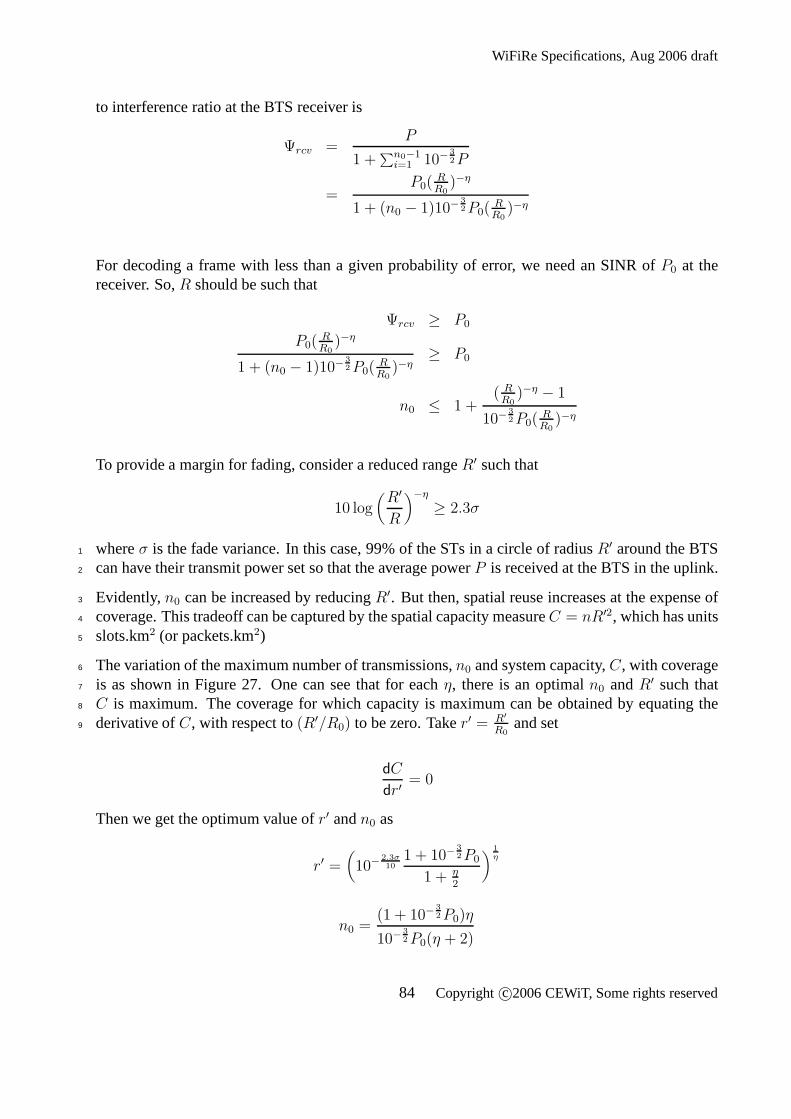
Evidently,n0 can be increased by reducingR′. But then, spatial reuse increases at the expense of3

coverage. This tradeoff can be captured by the spatial capacity measureC = nR′2, which has units4

slots.km2 (or packets.km2)5

The variation of the maximum number of transmissions,n0 and system capacity,C, with coverage6

is as shown in Figure 27. One can see that for eachη, there is an optimaln0 andR′ such that7

C is maximum. The coverage for which capacity is maximum can beobtained by equating the8

derivative ofC, with respect to(R′/R0) to be zero. Taker′ = R′

R0

and set9

dC

dr′= 0

Then we get the optimum value ofr′ andn0 as

r′ =(

10−2.3σ10

1 + 10−3

2 P0

1 + η2

)1

η

n0 =(1 + 10−

3

2 P0)η

10−3

2 P0(η + 2)



0 0.2 0.4 0.6 0.8 11

2

3

4

5

6

7

R’/R0

n0

η=4

η=3

η=2.3

0 0.2 0.4 0.61

2

3

4

5

6

7

R’/R0

n0

η=4

η=3

η=2.3

0 0.1 0.2 0.3 0.41

2

3

4

5

6

7

R’/R0

n0

η = 4

η=3

η=2.3

0 0.2 0.4 0.6 0.8 10

0.5

1

1.5

2

2.5

3

R’/R0

C

η=4

η=3

η = 2.3

0 0.2 0.4 0.60

0.2

0.4

0.6

0.8

1

R’/R0

n0

η=4

η=3

η−2.3

0 0.1 0.2 0.3 0.40

0.05

0.1

0.15

0.2

0.25

0.3

0.35

0.4

R’/R0

C

η=4

η=3

η = 2.3

Figure 27: Variation of the number of simultaneous transmissions possible (n0) and system capac-ity(C) with coverage relative to a reference distanceR0 for η = 2.3, 3, 4 andσ = 0, 4, 8. Plots forσ = 0, 4, 8 are shown left to right.

ση

0 4 8

2.3 0.77 0.31 0.123 0.78 0.39 0.204 0.80 0.47 0.28

η 2.3 3 4n0 3 3 4

Table 1: The optimum values ofC andn0 for different values ofη andσ.

Table 1 gives the optimum coverageC and maximum number of simultaneous transmissions pos-1

sible for different values ofηandσ. P0 is taken to be8dB. Directional gain of the antenna is taken2

to be 1 in the associated sector and−15dB in non-taboo directions. For path loss factorη = 4,3

the number of simultaneous transmissions is seen to be 4. Fora given value ofη, the maximum4

nunber of simultaneous transmissions is found to be independent of the fade varianceσ.5

1.2 Downlink6

In the downlink, the transmit power is kept constant. The BTSantennas transmit at a powerPt

times noise. LetR0 be the distance at which the average power received isP0 times noise.R be



the distance such that the average power received isP . Then,

P0 = Pt

(

R0

d0

)−η

P = Pt

(

R

d0

)−η

P

P0

=(

R

R0

)−η

Allowing n0 − 1 interferers,

Ψrcv =P

1 + (n0 − 1)10−3

2 P

=P0(

RR0

)−η

1 + (n0 − 1)10−3

2 P0(RR0

)−η

which is the same as in uplink. So, the optimum number of transmissions and optimum coverage1

in uplink and downlink are the same. The plots and tables for uplink apply for downlink also.2

1.3 Number of Sectors3

Once the maximum number of simultaneous transmissions possible,n0 is obtained, one gets some4

idea about the number of sectors required in the system. In ann0 sector system, when a transmis-5

sion occur in the taboo region between Sectorj and Sectorj +1, no more transmissions can occur6

in Sectorsj andj + 1. So, the number of simultaneous transmissions can be at mostn0 − 1, one7

in Sectorj andj + 1 and at most one each in each of the other sectors. Thus the maximum system8

capacity cannot be attained withn0 − 1 sectors. Withn0 + 1 sectors, one can choose maximal9

independent sets such that the sets are of cardinalityn0. So, at leastn0 + 1 sectors are needed in10

the system. From the spatial reuse model it can be seen that there can be up to 4 simultaneous11

transmissions in the system, for path lossη = 4. So, the system should have at least 5 sectors.12

2 Characterising the Average Rate region13

There arem STs. Suppose a scheduling policy assignskj(t) slots, out oft slots, to STj, such that14

limt→∞kj(t)

texists and is denoted byrj . Let r = (r1, r2, . . . rm) be the rate vector so obtained.15

Denote byR(n) the set of acheivable rates when the maximum number of simultaneous transmis-16

sion permitted isn. Notice that forn1 > n2, R1 ⊃ R2. This is evident because any sequence of17

scheduled slots withn = n2 is also schedulabale withn = n1.In the previous section, we have18

determined the maximum value ofn, i.e., n0. DenoteR0 = R(n0). A scheduling policy will19

aceive anr ∈ R0. In this section, we provide some understanding ofR0 via bounds.20



2.1 An Upper Bound on Capacity1

Suppopse each ST has to be assigned the same rater. In this subsection an upperbound onr isdertermined. In general, the rate vector(r, r, . . . r) /∈ R0. The upper bound is obtained via simplelinear inequalities. Consider the casen ≥ 3. Suppose one wishes to assign an equal number ofslotsk to each ST in the uplink. There areNU uplink slots in a frame. Consider Sectorj, whichcontainsmj STs. Thusk · mj slots need to be allocated to uplink transmission in Sectorj. WhenSTs in the interference regionj− or j+ transmit, then no ST in Sectorj can transmit. Supposekj± slots are occupied by such interference transmission. Now it is clear that

k · mj + kj± = NU

because whenever there is no transmission from the interference region for sectorj there can be atransmission from sectorj. Letmj− andmj+ denote the number of STs in the interference regionsadjacent to Sectorj. Since the nodes inj− andj+ can transmit together, we observe that

kj± ≥ max(k · mj−, k · mj+)

with equality if transmission inj− andj+ overlap wherever possible. Hence one can conclude2

that for any feasible scheduler that assignsk slots to each ST in the uplink3

k · mj + max(k · mj−, k · mj+) ≤ NU

For large frame timeN , divide the above inequality byN and denote the rate of allocation of slots4

by r. Thus if out oft slots, each ST is allocatedk slots, thenr = limt→∞kt≤ 15

r · mj + r · max(mj−, mj+) ≤ φu

whereφu is the fraction of frame time allocated to the uplink or

r ≤φu

mj + max(mj−, mj+)

This is true for eachj. So,6

r ≤φu

max1≤j≤n(mj + max(mj−, mj+))

For the casen = 2 for j ∈ {1, 2} denote the interfering nodes in the other sector bymj . One easilysees that

r ≤φu

max(m1 + m′1, m2 + m′

2)



2.2 An Inner Bound for the Rate Region1

In this section a rate setRL is obtained such thatRL ⊂ R′. i.e., RL is an inner bound to the2

aceivable rate set.3

The following development needs some graph definitions.4

Reuse constraint graph: Vertices represents links. In any slot all links are viewedas uplinks or5

all are downlinks. Two vertices in the graph are connected, if a transmission in one link6

can cause interference to a transmission in the other link. The reuse constraint graph is7

represented as(V, E), whereV is the set of vertices andE is the set of edges.8

Clique: A fully connected subgraph of the reuse constraint graph. Atransmission occuring from9

an ST in a clique can interfere with all other STs in the clique. At most one transmission can10

occur in a clique at a time.11

Maximal clique: A maximal clique is a clique which is not a proper subgraph ofanother clique.12

Clique incidence matrix: Let κ be the number of maximal cliques in(V, E). Consider theκ × mmatrixQ with

Qi,j =

{

1 if link j is in clique i0 o.w.

By the definition ofr andQ, a necessary condition forr to be feasible is (denoting by1, thecolumn vector of all1s.)

Q · r ≤ 1

since at most one link from a clique can be activated. In general, Q · r ≤ 1 is not sufficient toguarantee the feasibility ofr. It is sufficient if the graph is linear. A linear graph is one in whichlinks in each clique is contigous. A linear clique will have aclique incidence matrix of the form

Q =

1 1 1 1 . . . . . . 0 0 00 0 1 1 1 1 . . . 0 00 0 0 0 1 1 1 1 . . ....

...0 0 0 0 0 . . . 1 1 1

The reuse constraint graph in the multisector scheduling problem being considered has a ringstructure.Q · r ≤ 1 gives an upper bound on the rate vector. The reuse constraintgraph is linearexcept for the wrapping around at the end. If the nodes in one sector are deleted, the graph becomeslinear. Letmi be the set of STs in Sectori. There is a feasibleri such thatQ · ri ≤ 1 and all STsin mi are given rate 0. Linear combination of feasible vectors is also feasible. Thus, defining

RL := {x : x =m

∑

i=1

αirij ; Q · [r1r2 . . . rm] ≤ 1;m

∑

i=1

αi = 1; r1(m1) = . . . = rm(mm) = 0}

We see thatRL ∈ R13



2.3 Optimum Angular positioning of the Antennas1

As can be seen from the previous section, feasible rates set,R0, of the system depends on the spatial2

distribution of the STs around the BTS. Thus theR0 varies as the sector orientation is changed. A3

system where the antennas are oriented in such a way that mostSTs fall in the association region4

of BTSs rather than in the taboo region will have more capacity than one in which more STs are in5

the taboo regions.6

One sector boundary is viewed as a reference. LetR0(θ) denote the feasible rate set, when thisboundary is at an angleθ with respect to a reference direction. Then, for each0 ≤ θ ≤ 360◦

n, we

haveR0(θ), wheren is the number of sectors. SinceR0(θ) is not known, the inner boundRL(θ) isused in the following analysis. If each vectorr is assigned a utility functionU(r), then one couldseek to solve the problem

max0≤θ≤ 360◦

n

maxr∈RL(θ)

U(r)

and then position the antenna at this value ofθ.7

The optimization can be done so as to maximise the average rate allocated to each ST, with the8

constraint that each ST gets the same average rate. The boundevaluated with average rate to each9

ST, for antenna positions differing by5◦ is given below.ub(i) gives the upperbound on capacity10

of the system with antenna placed at((i − 1) ∗ 5)◦ from the reference line. Similarlylb(i) is the11

lower bound for each position.12

Upper bound,ub =[0.0714 0.0769 0.0714 0.0714 0.0667 0.0769 0.07140.0667 0.0667 0.0625 0.0625 0.0667 0.0667 0.0769]

13

Lower bound,lb =[0.0714 0.0769 0.0714 0.0714 0.0667 0.0769 0.07140.0667 0.0667 0.0625 0.0625 0.0667 0.0667 0.0769]

14

The bounds are seen to be very tight, and the maximum rate is obtained when antennas are at15

5◦, 25◦ or −5◦ from the reference line. The maximum rate so obtained is 0.0769, giving a sum16

capacity of 3.076. Only 14 different positions of the antenna are considered for a 5 sector system,17

since the pattern would repeat itself after that.18

Trying to optimize tha rates such that the rate to each ST is maximized will adversely affect the19

sum capacity of the system. So, takeU(r) =∑m

j=1(rj).20

For example, the sum capacity evaluated for antenna postition varied in steps of5◦ is as follows.21

It can be seen that the system capacity does not vary much withthe position of the antenna. But,22

there seems to be some positions which are worse than the others.23

Upper bound,ub = [4 4 4 4 4 4 4 4 4 4 4 4 4 4]24

Lower bound,lb = [4 4 3.8046 4 4 4 4 4 4 4 3.8883 3.8699 4 3.9916]25

Maximising∑m

i=1 log(r(i)) under the given constraints for upper bound and lower bound gives the26

utility functions for different positions of the antenna as27

Ulb =[−96.2916 −95.7459 −97.0998 −95.112 −95.9083 −98.0191 −96.1752−99.1991 −101.1465 −102.5186 −102.0872 −99.52350 −98.37440 −96.58240]

28



0 10 20 30 40 50 60 700

1

2

3

4

5

Orientation, θ (degrees)

Su

m o

f ra

tes to

ST

As (

no

. o

f slo

ts/s

lot tim

e)

Maximise Σ r

Maximise Σ log(r)

Equal rates

0 10 20 30 40 50 60 700

0.5

1

1.5

Orientation, θ (degrees)F

airn

ess in

de

x

Equal average rate

Maximize Σ log(r)

Maximise Σ r

Figure 28: Variation of sum rate and fairness index with antenna orientation for different utilityfunctions.

Uub =[−96.2916 −95.5485 −97.0998 −95.1122 −95.9083 −98.0191 −96.1752−99.1991 −101.1465 −102.5186 −102.0872 −99.5235 −97.3909 −96.4809]

1

2

The sum capacities for each of the rates above are bounded by3

Sum of rates for upperbound =[3.9102 3.8463 3.7333 3.8611 3.8535 3.6159 3.78963.6663 3.3637 3.30270 3.3513 3.6291 3.7565 3.7844]

4

Sum of rates for lower bound =[3.9102 3.8350 3.7333 3.8612 3.8535 3.6157 3.78963.6663 3.3636 3.3027 3.3512 3.6291 3.704 3.7734]

5

6

The utility function is maximum when the antenna is positioned at15◦ from the reference line.7

The sum of rates at this position is 3.86. This gives a trade-off between maximising the system8

capacity and providing fairness.9

The sum of the rate given to STs and the fairness index vs antenna orientation is plotted in Fig-ure 28. for different utility functions (the lower bounds are plotted here). Fairness index variesfrom 0 to 1. For a rate vectorr, the fairness index is given by

γ =(∑m

1=1 xi)2

m∑m

1=1 x2i

If the rates to different STs are equal, then fairness index would be 1, and it decreases as the rates10

are made unfair. The plots for maximum∑m

i=1 ri, maximum∑m

i=1 log ri are shown. It can be seen11

that maximising the sum rate gives high overall capacity, but poor fairness. On the other hand,12

maximising the average rate to each ST gives good fairness, but low sum capacity. Maximising13∑m

i=1 log ri gives a good tradeoff between maximising the system capacity and providing fairness.14

It is interesting to note that in maximum∑m

i=1 log ri case, the sum capacity is higher when fairness15

is lower and viceversa. For example, atθ = 10, we can see that the sum rate is close to 4. The16

fairness index is also close to 1. So, we may choose this orientation as optimum.17



ANNEX C: Scheduler Design1

1 Slot Scheduling2

The scheduling problem is the following.3

First partition the frame of sizeN slots into a contiguous part withND downlink slots and an uplink4

part withNU uplink slots, such thatND +NU = N−NB, whereNB is the number of slots required5

for the periodic beacon. Typically,ND ≫ NU as TCP data traffic is highly asymmetric since users6

download a lot more than they upload, and during downloads, long TCP packets (upto 1500 bytes)7

are received in the downlink and one 40 byte TCP ACK is sent in the uplink for alternate recieved8

packets.9

Now, whenmv,i, 1 ≤ i ≤ m, VOIP calls are admitted for STi, one needs to determine the number10

of slotsCi to be reserved in the uplink and downlink subframes for STi, such that the QoS targets11

are met for all the voice calls. For doing this, evidently theset of vectorsC = (C1, . . . , Cm) that12

are feasible (i.e., can be scheduled) needs to be known. For each deployment, there will be an13

optimal set of such vectorsCopt, and for any practical scheduler, there will be an achievable set of14

admissible vectorsC ∈ Copt.15

Once the required vector of voice payload slots has been scheduled, one has to schedule as many16

additional payload slots, so as to maximize the traffic carrying capacity for TCP while ensuring17

some fairness between the flows.18

1.1 Representation of a Schedule19

A feasible schedule for the deployment in Figure 29 is given in the table below, where each row20

stands for a sector and each colomn stands for a slots. There are 15 slots in the example. The entry21

in the table denotes the index of the ST that is transmitting in each sector in each slot. ST 1 in sector22

2 and ST 2 in sector 1 transmit for the first 4 slots. At the end of4th slot, ST 1 stops transmitting23

and ST 4 starts transmitting. The matrix representation of the schedule is also shown. The first24

3 columns stands for the 3 sectors. Each entry shows the indexof the ST that is transmitting.25

The last column indicates the number of slots for which that row is operative. Here, the sum of26

elements in column 4 is 15, indicating that there are 15 slots. This notation is followed throughout27

the examples.28

slots→29

2 2 2 2 2 2 2 2 0 0 0 0 0 0 01 1 1 1 4 4 4 4 4 4 4 4 4 4 40 0 0 0 0 0 0 0 6 6 6 6 6 6 6

2 1 0 42 4 0 40 4 6 7

30



��

��

��

��

��

��

BTS1

BTS2BTS3

STA1

STA2

STA4

STA5

STA6STA3

Figure 29: A system example showing the distribution of 6 stations in 3 sectors

1.2 A Greedy Heuristic Scheduler for the Uplink1

The STs are scheduled such that the one with the longest queueis scheduled first. Find an activation2

vector which includes the ST with the largest voice queue. Next include a non interfering ST with3

the longest queue and so on until the number of STs in the activation set is equal to the number of4

simultaneous transmissions possible or till the activation set is maximal. A maximal activation set5

is one to which one cannot add any more links such that there isno interference between the links6

in the set. Use this maximal activation vector until one of the STs in the set completes transmission.7

Once one of the STs complete transmission, we remove that ST from the set and schedule another8

ST, that does not interfere with the STs in the set. Repeat theprocedure until all the STs completes9

transmitting their voice packets. When all the STs completetheir voice transmission, the remaining10

slots are used for TCP transmission. If at any stage during voice transmission, a situation occurs11

where there are no more noninterfering STs in a sector which can transmit voice, but there is one12

that can transmit data, schedule data for that interval.13

In the beginning of each frame, for each slotk, heuristically build an activation vectoruk ∈ U14

starting from an ST in{i : qk,i = maxj qk,j}, i.e., the non interfering station with the maximum15

voice queue. Here,qkj denotes the queue length of thejth ST at the beginning of thekth slot. k16

varies from 1 toN over a frame. Build a maximal activation vector beginning with that link, and17

augmenting the vector every time with a non interfering link.18

I(u) denote the interference set of activation setu, the set of links that can interfere with the STs19

in u).20

Algorithm 1.121

1. Modify the voice queue lengths to include the overhead slots required. i.e., If an ST has a22

voice queue of 2 packets, add 3 slots of PHY overhead to make the queue length 5.23



2. Initially, slot indexk = 0. Let STi be such that

qki = maxl=1...m

{qkl}

i.e., The ST with longest voice queue at the beginning of slotk is i. Form activation vector1

u with link i activated. i.e.,u = {i}2

3. Let STj be such thatqkj = max

l{qkl : l /∈ I(u)}

j is such that it is the non interfering ST with maximum queue length. Augment s with link3

j. Now, findI(u) corresponding to the newu.4

4. Repeat step 3 until activation vector that we get is a maximal activation vector.5

5. Letn = {qkl : min

l=1,...,m(qkl, l ∈ u)}

i.e., n is the minumum number of slots required for the first ST inu to complete its trans-mission. Useu in the schedule fromkth to (k + n)th slot.

qk+n,i =

{

qk,i − n for i ∈ u′

qk,i for i /∈ u′

andk = k+n i.e., slot index advances byn, and the queue length for the STs at the beginning6

of k + nth slot isn less7

6. At the end ofk + nth slot,

u = u− {l : qkl = min(qkl, l ∈ u)}

i.e., remove from the activation vector, those STs that havecompleted their voice slot re-8

quirement.9

7. Go back to Step 3 and form maximal activation vector including u. Continue the above10

procedure untilq = 0 or n = NU In this step, we form a new activation vector with the re-11

maining STs in the activation vector (which need more slots to complete their requirement).12

8. Once the voice packets are transmitted, we serve the TCP packets in the same way, except13

that if in forming a maximal activation set, it is found that the only schedulable ST has only14

TCP packets to send, then TCP packets are scheduled.15

If q > 0 whenn = NU , the allocation is infeasible.16



1.3 A Greedy Heuristic Scheduler for the Downlink1

The difference of the downlink scheduling problem from the uplink scheduling problem is that in2

downlink, a transport block can contain packets to multipleSTs. By combining the voice packets3

to different STs to a single TB, we save considerable PHY overhead. For transmitting a single4

voice packet needs 4 slots, where 3 slots are for the PHY header. Transmitting 2 voice packets5

need only 5 slots. So, it is always advantageous to have transmissions in longer blocks. This can6

be done by grouping together the STs to those which are heard only by ith BTS, those heard by7

ith and(i− 1)th BTS, but associated to theith BTS and those heard byith and(i− 1)th BTS, but8

associated to the(i − 1)th BTS, for all values ofi.9

For example in Figure 30 STs 3 and 4 are associated with BTS 1 and hears only form BTS 1. So,10

any ST in the interference set of 3 will also be in the interference set of 4. Any transmission to11

ST 3 can equivalently be replaced by a transmission to 4. So, they form a group for the down12

likn schedule. Similarly, STs 8 and 9 are associated to BTS 2 and interfere with BTS 3. They are13

associated to the same BTS and cause interference to the sameSTs. So, ST 8 and 9 also form a14

group.15

��

STA12

��

STA5

��

STA6

��

STA9

��

STA10 ��STA11

��STA3

��

STA13

��

STA8

��

STA7

��

STA2

��

STA1

��

STA15

��

STA14

��

STA4

BTS1

BTS2

BTS3

Figure 30: Typical deployment of a system with 3 sectors and 15 STs

The STs are grouped together based on the above criterion. The queue length of each group would16

be the sum of queue lengths of the STs forming the group. The greedy heuristic scheduler for the17

uplink scheduling problem can then be used over these groups. This is made clearer in Example 2.318

1.4 Round Robin Scheduling19

A scheduler with least complexity can be designed as follows. The uplink and downlink parts of20

the frame may further be divided into two contigous parts. Alternate sectors are served in these two21

parts. For example, Sectors 1, 3, 5 are served in the first part, and Sectors 2, 4, 6 can be served in22

the second part of the frame. Interference between adjacentsectors can be eliminated in this way.23

With the number of sectors close to2n0, performance of this scheduler would be equivalent to that24

of the scheduler discussed in Section 1.2, since we can haven0 transmissions going on in each slot,25

with this scheduler. But, withn0 = 4, this would require 8 sectors in the system. With number26

of sectors less than2n0, the number of simultaneous transmissions would be less than n0 with the27

round robin algorithm, where as we can have upton0 transmissions with the greedy algorithm.28



1.5 Fair Scheduling1

Having all voice transmission in the beginning and data afterwards is wasteful in terms of overhead.2

Following the principle of having longer TBs, it is advantageous to have the voice and data tranfer3

to an ST in a block. To provide fairness to users, keep track ofthe average rates allocated to STs4

over time. The STs with low average rate over frames are givena chance to transmit first. Maximal5

independent sets are formed starting from the ST with the lowest average rate. Once the slots for6

voice transmission are scheduled, the attempt should be to have TCP transmission in blocks of size7

Tmax, so that PHY overhead per slot is minimised.8

LetRk be the vector of average rates allocated to STs till thekth frame andrk be the vector of ratesallocated to the STs in thekth slot, i.e, the fraction of slots allocated to STs in thekth frame. Theavrage rate acheived by the STs is obtained by computing the following geometrically weightedaverage.A large value ofα places lees weight on the previous frames.

Rk+1 = αRk + (1 − α)rk

1. Given a rate vectorR, obtain a maximal independent set as follows9

(a) u1 = {i1}10

i1 = arg min1≤j≤n Rj11

I(u1) is the set of links interfering with the links inu1. In this step, we select the ST12

with the smallest average rateRk for transmission.13

(b) Choosei2 ∈ arg min1≤j≤n,i2/∈I(u1) Rj14

u1 = {i1, i2}. In this step, we select one of the non interfering STs with minimum15

average rate for transmission.16

(c) Repeat the above until a maximal independent set is obtained. Now, we have a set17

with STs which have received low average rates in the previous slots. So, once all STs18

transmit their voice packets, we schedule these STs for datapackets.19

2. Let l1 denote the number of nodes inu1 at the end of step 1. Repeat the above for the20

remainingn−l1 nodes. Now we have a maximal independent set from the remainingNu−l121

nodes. If any one of thel1 nodes can be activated along with the maximal independent set22

formed from theNu − l1 nodes, add that till one get a maximal independent set. This yields23

u1,u2 . . .uk such that each node is included atleast once. Each node is included atleast once24

since a given number of slots is to be reserved for each ST in every frame.25

3. Now, we need to scheduleu1 for t1, u2 for t2, etc. To maximize throughput, we taketj =26

Tmax or number of voice slots required. The vectors in the initialpart of the schedule had27

low average rate over frames. So, they get priority to send data packets. So, starting from28

j=1, i.e., from the first activation vector, if the sum of number of slots allocated to STs in29

the frame is less thanNu, tj = Tmax. Else,tj = number of voice slots required.Therefore30

transmission takes place in blocks of length equal toTmax as long as it is possible.31

4. Update the rate vector asRk+1 = αRk + (1 − α)rk



2 Design Methodology: Examples1

The deployment considered in the examples are described by theA andI matrices given in Table 2.2

TheA matrix shows the BTS to which each ST is associated. Columns in both matrices correspond3

to sectors and rows correspond to STS.Aij = 1 indicates that theith ST is associated to thejth4

BTS. Each ST is associeted to one and only one BTS.Iij = 1 indicates that theith ST can hear5

from thejth BTS. An ST might hear from more than one BTS.6

Example 2.17

Equal Voice Load8

In this example there are 40 stations in 5 sectors. Any station within 72 ◦ is associated with the9

BTS and any station within32 ◦ of the center of a mainlobe can cause interference at that BTS.10

We take the maximum burst length,Tmax to be 15 andNU = 112. Voice packet ( including MAC11

header) is 44 bytes long. So, each voice packet requires one slot time for transmission. In this12

example, we taken0 = 4.13

Consider all stations to have the same voice slot requirement of 4 packets. The uplink transmission14

from each station could be done in a single block , which requires a total of 3 slots of overhead.15

So, the schedule should give at least 7 slots for each station. One schedule that attains this, (as16

obtained Algorithm 1.1) is given byS2.17

The first 5 columns of the matrixS2 gives the links that can transmit in each sector. A0 indicates18

that there cannot be a transmission by any of the stations in this sector without causing interference19

to at least one of the ongoing transmissions. The entries in the 6th column indicates the number of20

consecutive slots for which these vector is used in the schedule. The 7th column is the number of21

slots (over all the sectors) used for transmitting voice packets. The last column shows the number22

of slots, over all the sectors used for transmitting TCP packets.23

For example, consider the first row ofS2. This indicates that the ST 1 from Sector 1, 2 from Sector24

2, 11 from Sector 3, 6 from Sector 4 and none from Sector 5 are scheduled for the first 7 slots. At25

the end of 7 slots, the voice queues of these stations are exhausted, so we schedule other stations.26

FromS2, one sees that ST 40 gets a chance for transmission only in thelast row, i.e., by the 98th27

slot. It transmits till the 105th slot to complete transmitting its voice queue. This indicates that the28

scheduling of voice queues requires 105 slots.29

In the 1st row, ST 11 has been scheduled for 7 slots. So the voice queue of ST 11 is exhausted by30

the end of that row. But, since there are no other STs in Sector3, that can use the slot for voice31

transmission, we schedule ST 11 for TCP transmission further in the schedule. In this algorithm,32

priority is to STs that had been transmitting in the previousslot, and next priority to stations with33

lower index. But, better fairness can be ensured by round robining between the STs in a sector.34

Since the voice queue of ST 11 is exhausted by the end of 1st rowin S2 the ST 11 scheduled after35

1st row, i.e., from 29th slot is for TCP transmission. Similarly, ST 7 scheduled after the 11th row,36

ST 39 scheduled after 9th row etc. are for TCP transmission.37



A =

1 0 0 0 00 1 0 0 00 0 0 1 00 1 0 0 00 0 0 0 10 0 0 1 01 0 0 0 01 0 0 0 01 0 0 0 00 1 0 0 00 0 1 0 00 0 1 0 00 0 0 1 00 0 1 0 00 0 1 0 01 0 0 0 01 0 0 0 00 1 0 0 00 1 0 0 00 0 0 1 00 1 0 0 00 0 0 1 00 0 0 0 10 0 1 0 00 0 0 0 10 0 0 0 10 0 0 0 11 0 0 0 00 0 0 0 10 0 0 0 11 0 0 0 01 0 0 0 00 0 0 1 00 0 0 1 00 0 0 1 00 0 0 1 00 0 0 1 00 0 0 0 10 1 0 0 00 0 1 0 0

I =

1 0 0 0 10 1 0 0 00 0 0 1 10 1 0 0 00 0 0 0 10 0 0 1 01 0 0 0 01 0 0 0 01 0 0 0 11 1 0 0 00 0 1 0 00 0 1 0 00 0 0 1 00 0 1 1 00 0 1 0 01 0 0 0 01 1 0 0 00 1 1 0 00 1 0 0 00 0 0 1 10 1 0 0 00 0 1 1 01 0 0 0 10 0 1 0 00 0 0 0 10 0 0 1 10 0 0 0 11 0 0 0 00 0 0 1 10 0 0 0 11 0 0 0 01 0 0 0 00 0 0 1 10 0 0 1 00 0 0 1 00 0 0 1 00 0 0 1 00 0 0 0 10 1 0 0 00 1 1 0 0;

Q1 =

3234552445325245544532443553452545533254

S1 =

0 10 15 6 5 7 28 00 10 24 6 5 1 4 016 0 24 13 27 6 24 016 39 0 13 27 2 8 032 39 11 20 0 6 24 032 4 12 20 0 2 8 08 4 12 0 26 3 12 08 4 11 0 26 2 6 28 19 11 0 26 2 6 228 19 11 0 26 1 3 128 19 0 34 30 4 16 028 18 0 34 30 1 4 07 18 0 34 30 3 12 07 18 0 35 25 2 8 031 18 0 35 25 1 4 031 0 40 35 25 3 12 031 0 40 35 38 1 4 07 0 40 35 38 1 3 17 0 40 36 38 2 6 217 0 11 36 38 1 3 117 0 11 36 38 3 6 617 0 11 37 38 4 8 89 21 11 37 0 2 6 29 21 11 37 0 4 8 89 2 11 37 0 1 2 20 2 11 37 23 4 8 80 2 11 37 23 3 21 77 2 11 0 29 7 21 77 2 11 33 0 7 21 71 2 11 33 0 6 18 61 2 11 3 0 6 18 61 2 14 0 0 5 15 51 2 0 22 0 5 15 5

Q2 =

444...4

S2 =

1 2 11 6 0 7 28 07 4 12 3 0 7 28 08 0 15 13 5 7 28 09 19 24 34 0 7 28 00 10 11 35 25 7 28 016 21 14 0 27 7 28 017 0 11 36 30 7 21 728 18 0 37 38 7 28 031 39 11 20 0 7 21 732 39 0 22 5 7 21 70 39 0 22 23 7 7 147 39 11 0 26 7 7 217 39 11 0 29 7 21 77 39 11 33 0 7 21 77 0 40 33 0 7 14 7

Table 2: Data and results for the Example 2.1 and 2.2.Si is the schedule for voice slot requirementsgiven byQi, i ∈ {1, 2}. Note that the last two columns ofSi are the total number of slots in allsectors for voice and TCP packets respectively scheduled ineach row.



In this example, 4 STs transmit in each slot ( i.e.,3 × 26 slots of transmission.). Thereby, of the1

112 × 5 slots available ( since in each slot, at most one ST from a sector can transmit.),112 × 42

slots are used for transmission, giving a throughput of 78% and a goodput efficiency of 46%. In3

this schedule, transmission of TCP packets occur in 105 slots.4

Example 2.25

Unequal Voice Load6

Also given is the schedule obtained by the Algorithm 1.1, when the voice slot requirements are7

different for different stations. Given is one such vector (Q1) and the corresponding schedule (S1).8

In the example, in the first row, i.e., links 10,15,6,5 are scheduled for the first 7 slots. At the end9

of the 7th slot, ST 15 exhausts its voice queue. So, remove ST 15 from the vector, and add ST10

24 which can take its place. This continues till one of the other queues become empty. Then,11

remove the one whose queue is empty, and schedule some other ST which does not interfere with12

the ongoing transmissions, and so on till all STs are served.13

All the STs get a chance to transmit by the last row of the givenschedule. But, the last row finishes14

transmission by the 108th slot (as seen by summing up the lastcolumn ofS1). The slots from 10815

to 112 may be used for transmitting TCP packets for the STs in the last row. Here, the throughput16

78% and a goodput efficiency of 46%. In this schedule, transmission of TCP packets occurs in 14717

slots.18

Example 2.319

Downlink20

In downlink, transmission to multiple STs can be done in a block. In the deployment in this21

example, STs 2, 4, 19, 21, 39 all hear only from BTS 2. This can be seen from theA and I22

matrices. All these STs have 1 in the second column, indicating that they are associated to BTS23

2. TheI matrix has 1s only in the seccond column, indicationg that they hear only from BTS 2.24

These are grouped in tob. The transmissions to these STs can take place in a TB, since an ST25

which interferes with any ST inh will interfere with every other ST inh, and vice versa. So every26

ST in h is equivalent with respect to interference constraints. Anh occuring in the schedule in27

Table 3 indicates a transmission to this group of STs. The STswhich are in the same group are28

associated to the same BTS and are in the exclusion region of same sectors. The groups so formed29

for the example are given in Table 3. Similarly, the STs 3,20 and 33 hear from BTSs 4 and 5; all30

of them are associated to BTS 4. They are grouped toc. All STs in c are equivalent with respect to31

the interference constraints. The transmissions to these STs can occur in a TB. Now, the voice slot32

requirement of a group is the sum of the voice slot requirements of individual STs constituting the33

group. The same algorithm as for the uplink is then used over the groupsa, b, c, d, . . . with their34

respective queue lengths to obtain the schedule in downlink. Aggregating STs in the association35

and exclusion regions of each BTS like this has the advantageof increasing the overall system36

throughput, since transmissions occur in longer TBs. The goodput efficiency in downlink is about37

64%.38



Q2d =

22...2

S2d =

f b 0 e d 31f b h e 0 5f b h c 0 18a b h c 0 13f b h 0 n 130 g h 0 n 80 g i 0 n 8j 0 i 0 n 8f k 0 0 n 8f k 0 l d 80 k 0 l m 80 0 o e m 8

a = {1, 9} b = {2, 4, 19, 21, 39} c = {3, 20, 33}d = {5, 25, 27, 30, 38} e = {6, 13, 34, 35, 36, 37} f = {7, 8, 16, 28.31.32}g = {10} h = {11, 12, 15, 24} i = {14}j = {17} k = {18} l = {22}m = {23} n = {26, 29} o = {40}

Table 3: The part of the downlink schedule for completing thevoice slot requirement when 2 slotsare reserved for voice transmission from each ST.



ANNEX D: Simulation Analysis1

The fair scheduling algorithm and the round robin algorithmdiscussed in ANNEX C were imple-2

mented in MATLAB. The voice and data capacity of the system using these algorithms is provided3

in this section.4

1 Simulation Scenario5

We consider the distribution ofn STs inm sectors. Results for different values ofm andn are6

given. All STs are assumed to be carrying the same number of voice calls. One VOIP call requires7

one slot every alternate frame. A voice packet that arrives in the system is scheduled within the8

next two frames. If the system capacity and scheduling constraints do not allow the voice packet9

to be transmitted within two frame times of its arrival, the packet is dropped. In this simulation,10

we assume synchronous arrival of voice packets. i.e., if twovoice calls are going on from an ST,11

packets for both calls arrive synchronously, in the same frame. The data throughput considered is12

the saturation throughput, i.e., the STs have packets to be transmitted throughout. All STs have13

infinite queues and the schedule is driven by the average rates obtained over time. The STs which14

received low service rates in the previous frames are scheduled first.(See ANNEX C, Section 1.5)15

2 Numeric Results16

Following the fair scheduling algorithm described earlier, the data throughputs attainable forn STs17

in m sectors are calculated for different number of voice calls,widths of taboo regions,n andm.18

For each value ofn, m, width of taboo region (θ◦), and voice call requirement, the attainable data19

throughput is calculated in terms of fraction of downlink bandwidth, for 30 different deployments20

and the averages are tabulated. The minimum average throughput (in slots per slot time) attained21

among the STs, the maximum average throughput among STs, thesum of the average throughputs22

to STs and also the probability of a voice packet being dropped are tabulated.23

The first column of Tables 4 to 8 gives the number of sectors, number of STs, width of taboo region24

and the maximum number of simultaneous transmissions possible,n0. minrate is the minimum25

average rate over STs, averaged over random deployments,maxrate is the maximum average rate26

over STs,sumrate is the sum of average rates to STs, and the average fraction ofvoice packets27

dropped.28

For example, one can see from Table 4 that for 40 STs in 6 sectors, with a taboo region of width10◦29

andn0 = 3, the minimum average downlink throughput provided to an ST is 0.0507 of the down-30

link bandwidth. If one slot is reserved every two frames for voice calls, the downlink bandwidth31

being 66% of the total bandwidth of 11 Mbps, the ST gets 370 Kbps. Similarly, if two slots are32

reserved per ST every two frames, each ST receives an averageof at least 369 Kbps. The average33

fraction of voice packets dropped is zero when the number of STs is as small as 40.34



Number of voice calls per station

number of sectors,number of sSTs,

n0

width of taboo region, θ

1 2 3 4

6, 40,n0=3, θ = 10◦min d/l ratemax d/l ratesum d/l rates

0.05070.05572.1379

0.05040.05452.0909

0.04860.05382.0342

0.04530.05241.9766

min u/l ratemax u/l ratesum u/l rate

packet drop u/l

0.03370.07332.0641

0

0.02880.06361.8120

0

0.02770.05781.6330

0

0.02030.05111.4013

0


0.05070.05472.1086

0.04870.05522.0574

0.04720.05352.0171

0.04520.05281.9272


packet drop u/l

0.03470.07122.0544

0

0.02990.06641.8157

0

0.02380.05961.6002

0

0.01900.05471.3898

0


0.05260.06332.0865

0.04790.06132.0023

0.04720.05701.9881

0.04370.05981.9740


packet drop u/l

0.02980.08432.0484

0

0.02760.07591.8204

0

0.02080.07491.5909

0

0.01720.06241.3926

0


0.03260.03802.0792

0.03120.03592.0034

0.02970.03391.8873

0.02700.03221.7249


packet drop u/l

0.01370.04481.4863

0

0.00940.03571.2020

0

0.00500.02740.87140.0022

0.00260.01970.63680.0156


0.03250.03632.0472

0.03170.03681.9924

0.02930.03401.8861

0.02670.03211.7338


packet drop u/l

0.01300.04441.5189

0

0.00910.03981.2006

0

0.00550.02910.90360.0029

0.00180.01980.63270.0167


0.03380.03752.1148

0.03260.03582.0344

0.02930.03371.8997

0.02600.03181.7368


packet drop u/l

0.01390.04521.4985

0

0.00870.03601.1587

0

0.00490.03260.92990.0033

00.02570.63010.0179

6,80,n0=3,θ = 10◦min d/l ratemax d/l ratesum d/l rates

0.02440.02652.0453

0.02200.02711.9118

0.02000.02481.7390


packet drop u/l

0.00560.02451.0388

0

0.00250.01600.65630.0029

00.00910.35050.0229


0.02420.02672.0150

0.02240.02571.9039

0.02030.02631.7552


packet drop u/l

0.00480.02521.0604

0

00.01850.63050.0033

00.00970.33520.0312


0.02490.02682.0653

0.02280.02581.9339

0.02040.02401.7480


packet drop u/l

0.00450.02491.0319

0

0.00220.01740.67970.0042

00.01140.33990.0346

Table 4: The average throughput per ST averaged over 30 random deployments. The data through-puts are tabulated for different number of sectors, number of STs, width of taboo region andn0 = 3, 4. Throughputs are in terms of fraction of uplink or downlink bandwidth respectively





n0


1 2


0.01870.02192.0074

0.01680.02021.8184


packet drop u/l

0.00110.01460.6103

0

00.00680.27550.0250


0.01920.02172.0010

0.01740.02021.8327


packet drop u/l

0.00100.01290.59270.0017

00.00630.25760.0237


0.01940.02112.0005

0.01730.02051.8133


packet drop u/l

00.01420.58600.0037

00.00980.30400.0233


0.01550.01841.9903


packet drop u/l

00.00570.23050.0231


0.01570.01741.9538


packet drop u/l

00.00520.21770.0230


0.01390.01531.7393


packet drop u/l

00.00520.21170.0394

Table 5: The average throughput per ST averaged over 30 random deployments. The data through-puts are tabulated for different number of sectors, number of STs, width of taboo region andn0 = 3, 4(Contd)





n0


1 2 3 4


0.06580.08082.9443

0.06580.07822.8665

0.06610.07722.8532

0.06320.07772.7495


packet drop u/l

0.04520.12142.9113

0

0.03710.11252.6910

0

0.03330.10272.4730

0

0.02560.10292.3426

0


0.06160.08662.9434

0.06070.07562.7094

0.06060.07582.6901

0.05870.07082.5764


packet drop u/l

0.04050.14622.7302

0

0.03380.15262.4593

0

0.02670.14912.3504

0

0.02190.15132.1716

0


0.05500.06812.4473

0.05360.06662.3727

0.05300.06532.3198

0.04800.06902.1754


packet drop u/l

0.03260.11102.1184

0

0.02770.09231.8977

0

0.02270.09721.7520

0

0.01730.08661.5281

0


0.04690.05563.0059

0.04360.05522.8453

0.04040.04972.6891

0.03820.04732.5362


packet drop u/l

0.02330.06242.2345

0

0.01440.06021.8461

0

0.00880.05131.55980.0004

0.00220.04841.35670.0062


0.04650.05673.0010

0.04290.05472.8456

0.04010.05062.6901

0.03790.05002.5312


0.01920.09442.1408

0

0.01260.08701.7864

0

0.00690.07951.4975

0

0.00390.06951.29420.0083


0.03520.04692.3692

0.03340.04392.2139

0.03050.04192.0396

0.02830.03431.8635


packet drop u/l

0.01390.05211.5640

0

0.00780.04901.2581

0

0.00330.04170.9693

0

0.00180.03500.73190.0083


0.03330.04382.9465

0.03040.04132.7337

0.02820.03842.5300


packet drop u/l

0.01050.02921.4752

0

0.00690.02551.14930.0029

00.02360.91220.0283


0.03040.04212.8728

0.02880.03802.6641

0.0.02640.04082.4441


packet drop u/l

0.00690.03991.4386

0

0.00220.03891.12730.0025

00.04770.88100.0304


0.02560.03162.3167

0.02460.03092.0943

0.02090.02821.85944


packet drop u/l

0.00400.02631.0279

0

0.00160.02050.69970.0029

00.01550.43160.0254

Table 6: The average throughput per ST averaged over 30 random deployments. The data through-puts are tabulated for different number of sectors, number of STs, width of taboo region andn0 = 3, 4 (Contd)





n0


1 2


0.02600.03242.8934

0.02390.03012.6314


packet drop u/l

0.00350.01760.94220.0030

00.01050.65220.0250


0.02570.03322.8303

0.02260.03152.5684


packet drop u/l

0.00170.03180.97110.0023

00.02700.68030.0215


0.02100.02502.2563

0.01810.02401.9626


packet drop u/l

00.01590.60550.0010

00.01070.32800.0280


0.01840.02692.5225


packet drop u/l

00.00990.55290.0750

Table 7: The average throughput per ST averaged over 30 random deployments. The data through-puts are tabulated for different number of sectors, number of STs, width of taboo region andn0 = 3, 4 (Contd)

As the number of STs goes up to 80,n0 remaining as 3, one can reserve at most 2 slot per ST in al-1

ternate frames, with acceptable probability of dropping voice packets. With 80 STs, the probability2

of dropping a voice packet is more than 2 percent when we reserve slots for 2 calls per ST. With 803

STs, and slots reserved for one call per ST, each ST gets at least 123kbps of downlink bandwidth.4

But the uplink bandwidth is as small as 17 kbps. But, since theinternet traffic in predominantly5

downlink, the capacity required in the uplink is small.6

The rates given in Tables 4 to 8 are in terms of fraction of uplink of downlink bandwidth available7

for data transfer. Total uplink bandwidth is one third of 11 Mbps and downlink bandwidth is two8

thirds of 11 Mbps. So, a downlink rate of 0.0507 should be readas an uplink downlink bandwidth9

of a fraction of 0.0507 of11 × 23

Mbps. Similarly an uplink bandwidth of 0.0307 should be read10

as a fraction 0.0307 of11 × 13

Mbps. i.e.,11 kbps.11

As seen from the tables, with 6 sectors, andn0 = 3, the capacity remains almost the same irrespec-12

tive of the width of taboo region. This happens because even if the taboo region of a sector covers13

half of the adjacent sector, we can form maximal sets with 3 links. But, withn0 = 4, the capacity14

decreases with an increase in the width of taboo region. Witha taboo region of width30◦, in a 615

sector system, we can have at most 3 links scheduled at a time.16




no. of STs 1 2 3 4

min d/l rate 0.0531 0.0508 0.0479 0.0457

40 max d/l rate 0.0683 0.0657 0.0629 0.0604

sum d/l rates 2.2938 2.1899 2.0859 1.9813

min d/l rate 0.0344 0.0319 0.0295 0.0267

60 max d/l rate 0.0421 0.0390 0.0364 0.0341

sum d/l rates 2.2438 2.0875 1.9313 1.7750

min d/l rate 0.0255 0.0229 0.0202

80 max d/l rate 0.0296 0.0271 0.0245

sum d/l rates 2.1917 1.9833 1.7750

min d/l rate 0.0199 0.0172 0.0147

100 max d/l rate 0.0227 0.0202 0.0175

sum d/l rates 2.1396 1.8792 1.6188

min d/l rate 0.0110

120 max d/l rate 0.0132

sum d/l rates 1.4625

Table 8: The average data throughput per ST with round robin scheduler for number of sectors=6,number of STs 40, 60, 80, 100 and 120

Depending upon the antenna pattern and the terrain,n0 may go up to 4. Withn0 = 4, we can1

schedule slots for 2 calls per ST with a probability of voice packet dropping as small as 0.29%.2

The minimum, maximum and sum of average data throughput overSTs over different deployments3

are tabulated in Table 8 for the round robin scheduler, for different values of voice slot requirement.4

The average behavior of the round robin scheduler is almost the same as the greedy heuristics5

scheduler. But, in a given deployment, the greedy heuristicscheduler is found to be more fair.6

For example consider a deployment, where the adjacent sectors have 3 and 10 STs respectively.7

With a scheduler that round robins among the sectors, all STsin the sector with 3 STs will get8

1/3 of the downlink bandwidth, whereas all those in a sector with 10 STs get only 1/10 of the9

downlink bandwidth. But, if we were allowed to select the STsin the activation set based on queue10

lengths, or on average rates, with the condition that no two interfering transmissions are allowed11

simultaneously, it is possible to vary the fraction of time each sector is allowed to transmit, based12

on the number of STs in each sector (which will be reflected in queue lengths or average rates),13

and thereby provide better fairness.14



3 OPNET model and Simulation1

Development of an OPNET model for the WiFiRe protocol, including the fair scheduling algo-2

rithm, is ongoing. Such a development will not only be usefulto further understand the behaviour3

of the WiFiRe System under various conditions, but also may serve as a building block for the4

actual implementation of the protocol.5

A description of the preliminary work completed so far is given in this section. This makes the6

following assumptions: (i) The ST(s) and BS are initializedat the same time. No ranging is7

performed. (ii) BS after becoming ready, starts transmitting MAPs. Each ST receives MAPs and8

gets associated with the BS antenna from which it receives maximum power. (iii)Dynamic Service9

Addition messages are exchanged and the simulation starts;Dynamic Service Change messages are10

not supported at present.11

Figure 31: OPNET Model: WiFiRe MAC State Diagram

3.1 MAC State Diagrams12

Figure 31 shows the generic state diagram of the MAC. It showsstates common to both BS and13

ST. Different actions are taken in each state based on whether the node is the BS or an ST.14

In the Init State all variables are initialised. MAC and IP addresses are obtained. TheInvoke15

Corresponding Process State invokes abs control() module, in case the node is the BS. This16



state initializes the directional antennas (six in currentimplementation) and then enters theReady1

State to wait for events. In case the node is an ST, ast control() module is invoked. This2

orients the ST antenna towards the BS and then enters theReady State to wait for events.3

When the MAC (in theReady State) receives a packet from the higher layer, it makes transition to4

Enqueue State. Here, aclassify packet() module maps each incoming higher layer packet5

to one of the outgoing connections, identified by a CID. A CID has a queue associated with it.6

A get queue() module is invoked to determine the appropriate queue and thepacket is then7

inserted into it. A packet which does not match any conditionspecified in classifier is inserted in a8

default best-effort (BE) connection queue.9

When the MAC receives a data packet PDU from the PHY, it makes atransition to theProcess10

Data Packet State. Here the PDU is de-multiplexed into appropriate higher layer packets, based on11

the CID(s). These packets are passed to the higher layer for further processing.12

When the MAC receives a control packet PDU from the PHY, it makes a transition to theProcess13

Control Packet State. In case of the BS, this corresponds toDynamic Service Addition Request and14

Bandwidth Request messages. In case of the ST, this corresponds toDynamic Service Addition15

Response messages. When the BS receives aBandwidth Request message, the CID of the flow16

and the bandwidth requested are noted and the MAC returns to the Ready State. When the BS17

receives aDynamic Service Addition message, it determines the service flow type, assigns a CID18

and a queue. For UGS flows, anadmission control() module is invoked. This takes into19

account the UGS flow requirements and the number of free slotsper frame, to determine whether20

the flow can be admitted or not. An appropriateDynamic Service Response message is created.21

This is given to aschedule pk() module and the MAC returns to theReady State. When the22

ST receives aDynamic Service Response message, it creates a queue for the CID and returns to the23

Ready State. Note: One limitation of the simulation model implemented so far is that an ST needs24

to send all itsDynamic Service Addition Request messages at the start of the simulation itself.25

At a ST node, when a Beacon is received from the lower layer (PHY), it enters theProcess MAP26

State. A child st control process is invoked and the packet is passed to it. The processchecks27

each element in the UL-MAP. The each element in the UL-MAP contains: (i) CID, (ii) Start Slot28

(Slot number at which transmission should start) and (iii) Number of Slots (Number of slots alloted29

for transmission). If the CID in UL-MAP element belongs to that ST node, the number of slots30

allocated for transmission is checked and an appropriate number of packets are extracted from31

the queue associated with that CID. A MAC PDU (protocol data unit) is constructed, taking into32

account the PHY overhead and the PDU is given to aschedule pk() module. The control then33

returns from the child to the parentst control process which is returns to theReady State. This34

schedule pk() module independently transmits the PDU in the appropriate slot.35

The BS enters theProcess MAP State periodically, at the end of each frame (time interval). Here36

it invokes the scheduler, which takes into account the admitted UGS flows and pending band-37

width requests, to construct the DL-MAP and UL-MAP for the next frame. It then constructs data38

PDU(s) for downlink transmission in the next frame, based onthe DL-MAP. This is similar to the39

mechanism followed by the ST.40



4 Simulation Setup1

A preliminary validation of the WiFiRe OPNET model was carried out using the scenario shown2

in Figure 32. The scenario consists of one BS, surrounded by 16 ST(s), which are placed randomly3

around the BS. Each ST has 4 flows registered at the BS: one UGS downlink flow, one UGS uplink4

flow, one BE downlink flow and one BE uplink flow. The following parameters can be specified5

while setting up the simulation: (i) Classifier Definition, (ii) Service Class Definition, (iii) Packet6

inter-arrival time (exponential distribution) and (iii) Packet size (Uniform Distribution).7

Figure 32: Simulation scenario; unit 5 km.Figure 33: Throughput (on Y-axis in bps) v/sLoad (on X-axis in 10 Mbps)

Figure 34: Delay of UGS flows (on Y-axisin seconds) v/s Throughput (on X-axis in 10Mbps)

Figure 35: Delay of BE flows (on Y-axis in sec-onds) v/s Throughput (on X-axis in 10 Mbps)



Figure 33 shows how throughput of system varies with increasing load, while Figure 34 and Fig-1

ure 35 show the delay v/s throughput for UGS and BE flows, respectively. The behaviour observed2

in graphs is close to that expected by simple theoretical analysis, thereby validating the WiFiRe3

OPNET model developed so far. Further development of the model as well as detailed experimen-4

tation is underway.5

References6

[1] Ashok Jhunjhunwala, Anand Kannan and Bhaskar Ramamurthi. Interim Broadband Wireless7

System for India. CEWiT Technical Report, CEWiT-2005-02, March 2005, available from8

http://www.cewit.org.in/9

[2] Broadband Policy 2004. Govt. Of India, Ministry of Communications and10

Information Technology, Department of Telecommunications, available from11

http://www.dotindia.com/ntp/broadbandpolicy2004.htm12

[3] J. Klutto Milleth and Bhaskar Ramamurthi. Study of Imminent and Emerging Broadband13

Wireless Technologies. CEWiT Technical Report, CEWiT-2005-01, March 2005, available14

from http://www.cewit.org.in/15

[4] Digital cellular telecommunications system (Phase 2+)(GSM);GSM Release 1999 Specifi-16

cations. available from http://www.etsi.org/17

[5] Digital cellular telecommunications system (Phase 2+)(GSM);General Packet Radio Service18

(GPRS) Release 1999 Specifications. available from http://www.etsi.org/19

[6] cdma2000 Specifications. available from http://www.3gpp2.org/20

[7] iBurst Specifications. available from http://www.arraycomm.com/docs/iBurst.pdf21

[8] Flash-OFDM Specifications. available from http://www.flarion.com/products/flashofdm.asp22

[9] corDECT, ”Wireless access system”. Technical report ofMidas Communication Technolo-23

gies Private Ltd. December 2000.24

[10] IEEE Std 802.16-2004. IEEE Standard for Local and metropolitan area networks ”Part 16:25

Air Interface for Fixed Broadband Wireless Access Systems”. (Revision of IEEE Std 802.16-26

2001), 2004.27

[11] IEEE Std 802.11-1999. IEEE Standard for Local area networks ”Part 11: Wireless LAN28

Medium Access Control (MAC) and Physical Layer (PHY) specifications”. 1999.29

[12] Pravin Bhagwat, Bhaskar Raman and Dheeraj Sanghi. Turning 802.11 Inside-Out.ACM30

SIGCOMM Computer Communication Review, 34(1):33–38, Jan 2004.31

[13] Leena Chandran-Wadia, Shruti Mahajan and Sridhar Iyer. Performance of 802.11 Wireless32

LANs. IEEE Conference on Computer Communications, Mumbai,2002.33

[14] http://www.smartbridges.com/products/ap2np.asp34

[15] http://www.brovis.com/files/productas1000.htm35

[16] http://www.cisco.com/en/US/products/hw/wireless/ps5279/36

[17] http://www.winncom.com/moreinfo/item/ETHERANT-3-20/index.html37

[18] IEEE Std 802.1F-1993. IEEE Standards for Local and Metropolitan Area Networks: Com-38

mon Definitions and Procedures for IEEE 802 Management Information, 1993.39

[19] Digital enhanced cordless telecommunications (DECT). ETSI EN 300 175, 1988. available40

from http://www.etsi.org/41



[20] Broadband Radio Access Networks (BRAN); Requirementsand architectures for broadband1

fixed radio access networks (HIPERACCESS). ETSI Technical Report TR 101 177 V1.1.1,2

May 1998.3

[21] Anurag Kumar, D.Manjunath and Joy Kuri.Communication Networking, An Analytical Ap-4

proach. Morgan Kaufman Networking Services, Elsevier, 2004.5

[22] Atilla Eryilmaz, R.Srikant and R.Perkins. Stable Scheduling Policies for Wireless Fading6

Channels. IEEE/ACM Transactions on Networking, 2005.7

[23] Arash Behzad and Izhak Rubin. On the Performance of Graph Based Scheduling Algorithms8

for Packet Radio Networks. GLOBECOM, 2003.9

[24] Dimitri P. Bertsekas.Dynamic Programming and Optimal Control, volume 1. Athena Scien-10

tific, 2001.11

[25] Sem Borst, Ken Clarkson, John Graybeal, Harish Viswanathan, and Phil Whiting. User-12

Level QoS and Traffic Engineering for 3G Wireless 1xEV-DO systems. Bell Labs Technical13

Journal, 8(2):33–47, 2003.14

[26] Harish V. Shetiya. Efficient Routing and Scheduling forIEEE 802.16 Mesh network. Master’s15

thesis, Electrical Communication Enigineering, IISc, 2005.16

[27] Leandros Tassuilas and Anthony Ephremides. Stabilityproperties of constrained queuing17

systems and scheduling policies for maximum throughput in multihop radio networks. IEEE18

Transactions on Automatic Control, 1992.19

[28] Bhaskar Raman and Kameswari Chebrolu. Revisiting MAC Design for an 802.11-based20

Mesh Network. Third Workshop on Hot Topics in Networks, San Diego, Nov 2004.21

[29] E. Brewer, M. Demmer, et. al. The case for Technology in Developing Regions. IEEE22

Computer, June 2005, pp. 25-38.23

[30] M.J. Lee, J.L. Zheng, Y-B. Ko and D.M. Shreshta. Emerging standards for wireless mesh24

technologies. IEEE Wireless Communications, April 2006, pp. 56-63.25


annex a : design drivers 1 the indian rural scenariosri/projects/wifire/wifire-annex-lines.pdf ·...

Documents