another look at travel patterns and urban form: the us and
TRANSCRIPT

Another look at travel patterns and urban form: The US and Great Britain
Genevieve Giuliano* School of Policy, Planning and Development RGL 216 University of Southern California Los Angeles, CA 90089-0626 Phone 213-740-3956 Fax 213-740-0001 [email protected] Dhiraj Narayan School of Policy, Planning and Development University of Southern California Los Angeles, CA 90089-0626
*Contact Author
2 GENEVIEVE GIULIANO ET AL
Summary: This paper explores the relationship between land use patterns and individual mobility from a comparative international perspective. There is a vast literature on US automobile dependence. Major explanatory factors include: transportation, housing, land use and tax policy; per capita incomes; American cultural preferences; national geography; and spatial structure of US metropolitan areas (itself a result of the first three factors). Emphasizing the policy environment, many researchers have cast their analysis in comparative terms, noting the differences in automobile use between European countries and the US. It is argued that US patterns of metropolitan form, with low development densities and dispersed population and employment, reinforce auto dependence. In contrast, most European metropolitan areas, with higher densities and more centralized land use patterns, have lower levels of auto use. Stronger controls on land use employed in many European countries are seen as having preserved the compact form of metropolitan areas. These arguments imply significant relationships between land use patterns and travel behavior. Using travel diary data from the US and Great Britain, we compare these relationships across the two countries. We find that differences in daily trips and miles traveled are largely explained by differences in household income. High density is associated with less travel in the US, but not in Great Britain, likely the result of greater spatial concentration of low income households in the US and higher quality public transport in Great Britain.
ANOTHER LOOK AT TRAVEL PATTERNS AND URBAN FORM 3
1. Introduction The relationship between transportation and land use continues to be of great
interest to urban researchers across many disciplines. This relationship is also a public
policy issue of growing importance. Automobile dependence is a major topic in
sustainability discussions, and it is linked to the growth of dispersed, low density
patterns of urban development. This paper explores the relationship between land use
patterns and individual mobility from a comparative international perspective. Using
individual travel diary data for the US and Great Britain, we present some preliminary
results on travel patterns and their relationship with basic measures of urban form.
2. Literature Review
There is a vast literature on US automobile dependence. Decades of research
by geographers, economists, historians, and others have generated a widely accepted
set of explanations for the US situation (e.g. Muller 1981; Pucher, 1988; Jackson
1985). Major factors explaining US auto dependence include: 1) transportation,
housing, land use and tax policy, 2) per capita incomes, 3) American cultural
preferences, 4) national geography, and 5) spatial structure of US metropolitan areas
(itself a result of the first three factors). The major emphasis has been on the policy
environment. Many researchers have cast their analysis in comparative terms, noting
the differences in automobile use between European countries and the US (Dunn,
1981; Pucher, 1988; Pucher and Lefevre, 1996; Nivola, 1999). Pucher (1988), for
example, provides a list of the key policies that affect the price and convenience of
auto ownership and use. Recent research has focused on the role of land use patterns.
4 GENEVIEVE GIULIANO ET AL
It is argued that US patterns of metropolitan form, with low development densities and
dispersed population and employment, reinforce auto dependence. In contrast, most
European metropolitan areas, with higher densities and more centralized land use
patterns, have lower levels of auto use. It is argued that stronger controls on land use
employed in many European countries have preserved the compact form of
metropolitan areas (Cervero, 1995; Bernick, and Cervero 1997; Pucher and Lefevre,
1996; Newman and Kenworthy, 1998). Of course, land use patterns are the outcome
of historical development patterns, which are in turn a function of policy, economic
factors, technology, and culture.
However, when we compare trends over time, we find that automobile
ownership and use is increasing in both the US and in Europe, and that the rate of
increase over the past two decades has been greater in several European countries than
in the US (Giuliano, 1999; Orfeuil and Salomon, 1993; Pucher and Lefevre, 1996). In
addition, urban growth patterns in Europe are showing forces of decentralization, with
central cities losing employment share, and more rapid growth occurring in suburbs
(Gillespie,1999; Hansen,1993). That is, countries with far different policy
environments than the US are experiencing the same phenomena, albeit from a very
different base and under different economic and social circumstances.
Trends of the past two decades call into question our conventional
understanding of auto dependence. Countries with far less “auto friendly” land use
patterns, and with policies that make auto use much more costly and impose far more
control on land use patterns are experiencing continued growth in auto ownership and
ANOTHER LOOK AT TRAVEL PATTERNS AND URBAN FORM 5
use. A cross national projection of car ownership by Dargey and Gately (1997) show a
continuation of substantial increases in car ownership in most European countries but
relatively little increase for the US.
Trend data suggest that policy factors may not be as important as once thought.
Transportation economists have long argued that per capita income is the single most
important explanatory factor in auto ownership and use (Meyer and Gomez-Ibanez,
1981; Lave, 1996; Ingram and Liu, 1999). The effectiveness of policies that affect the
price of auto ownership and use declines as relative income increases. Value of time
increases with income, effectively offsetting the higher monetary costs of faster modes
and increasing demands for such modes. In addition, economic restructuring has
changed firm location patterns in response to shifts in agglomeration benefits (spread
of agglomeration economies over greater spatial distances due to reduced transport and
communications costs), and the shift to an information-based economy allows more
activity to be “footloose” (Kasarda, 1995; Chinitz, 1991; Kutay, 1988a, 1988b).
Moreover, the ability of governments to impose constraints on auto ownership and use
may decline as globalization proceeds and location freedom increases.
Although there are many international studies of travel patterns, these do not
explicitly address transportation and land use relationships.1 International comparative
research on transportation and land use has to date been limited either to aggregate
comparisons using national data or to qualitative discussions. Aggregate comparisons
include the various Newman and Kenworthy studies (1989a, 1989b, 1998). These

6 GENEVIEVE GIULIANO ET AL
studies compare per capita gasoline consumption and metropolitan densities, and find a
non-linear relationship of increasing per capita gasoline consumption with declining
density. Their work has been criticized, primarily because per capita fuel consumption
is an indirect measure of auto travel, and because they fail to account for many other
factors that affect automobile use, such as the employment rate or household size
(Gordon and Richardson, 1989; Gomez-Ibanez, 1991). Schafer and Victor (1998)
presented a travel budget model with time and money constraints, and showed that
these are stable over space and time. They projected future levels of mobility and
modal use across 26 countries. Their work does not address land use factors and is
based on national averages.
Pucher and Lefevre (1996) provide an overview of travel trends across several
European countries, and discuss differences in terms of policy, geography and cultural
factors. Among the numerous and complex factors that may account for differences,
they note the greater proportion of population living in central cities, more restrictive
land use and automobile policies, and a greater consensus among voters and politicians
to control the negative impacts of the automobile. Nivola, (1999) explains the sprawl
of US metropolitan areas vs compact urban form of European countries by 13
“determinants” ranging from national geographic and demographic differences to
differences in tax policy. Giuliano (1999) describes travel and land use trends in the
US and several European countries, and argues that rising per capita incomes,
changing demographics, and economic restructuring explain trends in travel patterns in
1 For example, see Orfeuil and Salomon, 1993.
ANOTHER LOOK AT TRAVEL PATTERNS AND URBAN FORM 7
both the US and Europe. An exception to these mainly descriptive studies is the Clark
and Kupers-Linde (1994) comparison of commuting patterns between the Los Angeles
Metropolitan Area and the Randstaad region of The Netherlands. Comparing shifts in
commuting patterns over time, Clark and Kupers-Linde show that commute flows have
lengthened and dispersed in both metropolitan regions (despite very different policy
environments). These shifts are attributed to economic restructuring and the
emergence of polycentric spatial form.
Comparisons across national aggregates ignore within-country variations that
might be important explanatory factors. For example, some countries are more
urbanized than others, or have older population age profiles, and both these factors are
known to affect travel behavior. In addition, aggregate patterns are the outcomes of
individual decisions regarding where, when, how and with whom to conduct daily
activities. Hence understanding differences in aggregate travel patterns requires
understanding differences in disaggregate travel patterns.
3. Research Approach
In examining the role of land use factors, what is the appropriate measure of
travel? In a previous paper (Giuliano 2002), we have argued that appropriate measures
should capture travel for all purposes and by all modes. Total travel can be measured
in terms of trips, distance and time. Trips capture the total number of activities
conducted, but provide limited information. The more interesting question is where
people choose to shop or work. The spatial range of travel over the course of the day is
8 GENEVIEVE GIULIANO ET AL
captured by distance and time. Of these, distance is the more appropriate measure of
mobility.
Travel time is problematic, because it is determined by both distance and
speed. Higher travel speed is better, all else equal, as it reduces the time cost of
traveling a given distance. Nonetheless, low travel speed may indicate spatial forms
(mainly high density development) that provide higher levels of accessibility, and may
provide additional insight on transportation – land use relationships. In this paper,
however, we restrict the analysis to total daily trips and total daily travel distance.
Our basic question is, what explains differences in travel patterns – particularly
automobile use – between the US and the countries of Europe? More specifically,
what is the role of land use characteristics? The literature shows that travel is a
function of individual and household characteristics, household transportation
resources (car availability, driver’s license), transportation prices and supply
characteristics, and land use. If we assume that individuals are rational utility
maximizers, it follows that similar people should have similar behavior, all else equal.
For example, household income or the individual’s age should have a consistent
relationship to travel across the two countries. However, cultural differences may
promote differences. For example, if older adults are more likely to live with extended
family in Europe, we might expect lower levels of trip making, since household
maintenance activities are shared among more people.
Car availability is mainly a function of the costs of ownership and use.
Possession of a driver’s license a function of the historical trajectory of car ownership.
ANOTHER LOOK AT TRAVEL PATTERNS AND URBAN FORM 9
In many European countries women are less likely than their US counterparts to have a
driver’s license, and the difference increases with age. Transportation supply and price
characteristics should work the same way across individuals, but differences between
countries should lead to comparable differences in travel patterns. Prior research has
shown that higher costs of car purchase, fuel and parking are associated with relatively
less car use. Land use is considered a major factor, as the distribution of activities in
space determines accessibility. Higher densities in European metropolitan areas should
be associated with relatively less car use and more use of public transit and non-
motorized modes. Similarly, the greater availability of public transport in large
metropolitan areas, together with congestion and higher parking costs, should be
associated with less car use.
The present research addresses mobility, or the total amount of travel a given
person conducts over the course of a day, by all modes, both motorized and not
motorized. The general model is,
( )LTXfY ,,=
(1)
Where
Y = daily mobility
X = attributes of the individual
T = transportation resources available to the individual
L = attributes of the residential location

10 GENEVIEVE GIULIANO ET AL
The X variables include the main characteristics associated with travel, such as
age, gender, employment status, household composition, and household income.
Transportation resources include driver’s license and car availability. Location
attributes include density and metropolitan location. How should country differences
be incorporated into this model? The question is whether observed differences
between countries remain, once socio-economic and geographic factors are controlled.
We use dummy variables to test both independent and first order interaction effects.
The model to be estimated is therefore:
Y = f(X, T, L, XR, TR, LR, R),
(2)
Where R = country dummy.
What about differences in transportation supply and pricing? We know that
indicators such as road mileage or fuel prices differ greatly across countries, and these
differences will be picked up by the country dummy variable. The question is, are
differences within each country so large that these factors should be taken into
account? At this time suitable data are not available at the regional level, hence we
leave this question for subsequent analysis.
There is also a question regarding how car ownership should be incorporated
into the model. Car ownership depends on price as well as demand for travel, and

ANOTHER LOOK AT TRAVEL PATTERNS AND URBAN FORM 11
hence is endogenous to daily mobility. Therefore a simple OLS regression model
based on (2) above will be biased. One way to avoid this problem is to estimate a
reduced form model, omitting car ownership variables. On the other hand, we could
argue that daily travel is the outcome of short-run decisions, given a series of longer
run choices about car ownership, employment and residential location, hence it is
reasonable to include car ownership variables in the model. In this paper we present
results for both approaches.
4. Data
International comparisons must begin with the fundamental question of what
to compare. In our case the decision was made for practical reasons. We want to
eventually include several European countries in our research, but the difficulties of
generating comparable data sets constrained us to beginning with just one European
country, Great Britain. We had access to travel diary data and to the government staff
who managed the survey. We were therefore able to work through the many
challenges of understanding the data and making the necessary changes to generate
comparable data sets. From an analytical standpoint, Great Britain represents a
reasonable representation of a “European country,” in that widespread car ownership
occurred well after World War II, its central cities are dense, pedestrian oriented and
well served by public transit, auto ownership and use costs are relatively high, and land
use controls are relatively strong. It is also important to note the large fundamental

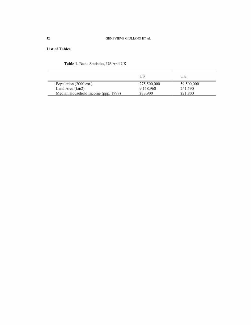
12 GENEVIEVE GIULIANO ET AL
differences between the two countries in terms of population, size, and household
income, as illustrated in Table 1.
The NPTS and NTS
We use the US 1995 Nationwide Personal Travel Survey (NPTS) and the UK
1995/97 National Transport Survey (NTS). Both are household-based surveys that
elicit travel diary information from all members of the household.2 The NPTS was
conducted for the first time in 1969 to develop a database of basic travel information
for the US. Households are selected via a complex stratified sampling method, and all
members five years old or older of the selected households are interviewed.
Information on household characteristics, individual characteristics, car ownership and
use is collected. The 1995 NTPS included 42,000 households, of which half are from
states or metro areas that paid to have their area over-sampled. Households were
assigned a 24 hour "travel day" and a 14 day "travel period". The survey data are
weighted to account for sample design and selection probability, non-response bias and
non-coverage bias.3
The NTS is a series of household surveys designed to provide a national bank
of personal travel information for Great Britain. The Ministry of Transport
2 Specifically, all persons 5 years or older are included in NPTS; all persons of all ages are included in NTS.
3 The weighting is developed for households. The household weights are based on time of year, geographic region, race/ethnicity, and household size. Person weights are calculated from the household weight, adjusted for non-responding members of responding households. Trip weights are calculated based on the person weights. The weights are scaled to the total US 1995 population.

ANOTHER LOOK AT TRAVEL PATTERNS AND URBAN FORM 13
commissioned the first NTS in 1965. The NTS is based on a random sample of private
households, and is limited to Great Britain (England, Wales, Scotland). In order to
select the appropriate number of addresses, a stratified multi-stage random probability
sample is used. Seven day travel diaries are kept by each member of the household,
with adults reporting for younger children and others unable to provide information on
their own behalf. Data collected include information on: household, individuals,
vehicles, long-distance journeys (including those made in the three weeks before the
start of the seven day travel week), journeys made during the travel week, and stages of
journeys made during the travel weeks. The NTS makes a special effort to include
'short walks', e.g. walks trips of less than 1 mile. Respondents are asked to include
these trips on Day 7 of the diary only. The NTS data are not weighted. The sample is
presumed representative of the population based on the way the sample is chosen. The
NTS is conducted on an ongoing basis; the “1995” survey was conducted from 1995
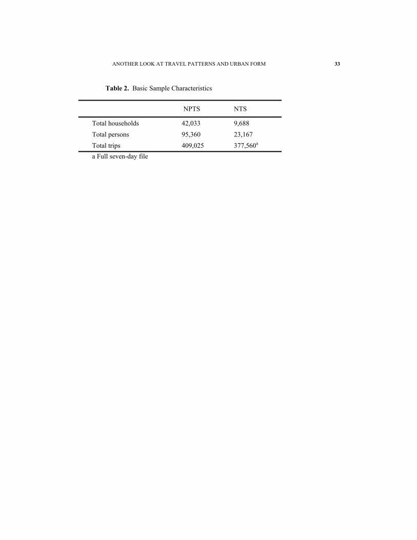
through early 1997. The NTS sample included 9,688 "fully co-operating" households
in 1995/1997.4 Basic characteristics of the two samples are given in Table 2.
After extensive data cleaning and adjustments to assure comparability across
the two samples, we created a pooled sample randomly drawn from the two surveys.
Preliminary analysis revealed that using only the Day 7 NTS data was the best
alternative for generating comparable person level travel diary files.5 Once these files
were created, we drew random samples from each file to generate a 50/50 pooled
4 A fully cooperating household has completed all basic survey questions and each household member has completed the 7 day diary.
5 See Giuliano, Hu and Narayan (2000) for details.

14 GENEVIEVE GIULIANO ET AL
sample. Because of the difference in sample size, the selection ratio was 1 in 9.5 for
the US and 1 in 2.3 for GB. The US sample was drawn from the weighted file, and
weights were preserved in the pooled sample. We use the 1995 OECD purchasing
power parity of 0.6539 to convert GB household income data to US dollar values.6
Measures of Urban Form
Empirical research is often constrained by data availability. Much of the
literature on urban form, for example, is based on measures of population because
population data is widely available. Comparative research is typically even more
constrained because of the difficulties involved in obtaining data in comparable spatial
units. For these reasons we are limited to two measures of urban form: metropolitan
size and population density. Metropolitan size is a rough proxy measure of
accessibility and urban structure. Smaller metropolitan areas (those under 500,000
population) tend to be self-contained, with one main center. Larger metro areas are
more likely to polycentric and hence have more cross-commuting. The largest metro
areas, particularly those with large downtowns, have the greatest potential for high
levels of daily travel due to long average commutes and high accessibility over an
extensive area. In contrast, non-metropolitan areas may be very self-contained (there
is nowhere to go outside one’s village), or many generate fewer but longer trips due to
very limited accessibility. Metropolitan size is measured in the US by Metropolitan
Statistical Area (MSA) and by Consolidated Metropolitan Statistical Area (CMSA).
6 http://www.oecd.org/std/pppoecd.xls

ANOTHER LOOK AT TRAVEL PATTERNS AND URBAN FORM 15
For Great Britain, we developed a comparable measure by using 1991 British Census
population figures and the household residence location data.
In the US, population density, when measured at a sufficiently disaggregate
level, has proven to be an effective proxy for intra-metropolitan spatial structure (e.g.
Pushkarev and Zupan, 1977; Niemeier and Rutherford, 1994; Schimek, 1996). High
density is a surrogate for greater transit availability, more walkable environments,
mixed use, and high accessibility. Low density is a surrogate for low accessibility.
Population density may not be as useful a measure for Great Britain, given the
generally greater availability of what might be termed high “local accessibility” areas.
We measure density at the most disaggregate level possible with our data. For the US,
the spatial unit is the census tract; the spatial unit for GB is the Local Area, generally
larger than US census tracts.
Sample Characteristics
There are substantial differences between the US and GB in demographic and
socio-economic characteristics. The age distribution for GB has both more children
(expected due to including children of all ages in the sample) and a larger share of
older persons. There are relatively more persons in two or more adult households
with children in the US, but more multiple adult households without children in GB.
There are also relatively more multiple adult retired households in the US. Household
income is much lower in GB, as was shown in Table 1. All of these differences
suggest lower rates of travel for GB, all else equal.
16 GENEVIEVE GIULIANO ET AL
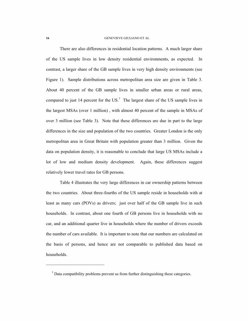
There are also differences in residential location patterns. A much larger share
of the US sample lives in low density residential environments, as expected. In
contrast, a larger share of the GB sample lives in very high density environments (see
Figure 1). Sample distributions across metropolitan area size are given in Table 3.
About 40 percent of the GB sample lives in smaller urban areas or rural areas,
compared to just 14 percent for the US.7 The largest share of the US sample lives in
the largest MSAs (over 1 million) , with almost 40 percent of the sample in MSAs of
over 3 million (see Table 3). Note that these differences are due in part to the large
differences in the size and population of the two countries. Greater London is the only
metropolitan area in Great Britain with population greater than 3 million. Given the
data on population density, it is reasonable to conclude that large US MSAs include a
lot of low and medium density development. Again, these differences suggest
relatively lower travel rates for GB persons.
Table 4 illustrates the very large differences in car ownership patterns between
the two countries. About three-fourths of the US sample reside in households with at
least as many cars (POVs) as drivers; just over half of the GB sample live in such
households. In contrast, about one fourth of GB persons live in households with no
car, and an additional quarter live in households where the number of drivers exceeds
the number of cars available. It is important to note that our numbers are calculated on
the basis of persons, and hence are not comparable to published data based on
households.
7 Data compatibility problems prevent us from further distinguishing these categories.

ANOTHER LOOK AT TRAVEL PATTERNS AND URBAN FORM 17
5. RESULTS
Results are presented in two parts. First, we give some basic descriptive
statistics on travel characteristics. Then we present results from regression models.
Travel Characteristics
We begin by presenting some descriptive information on travel characteristics.
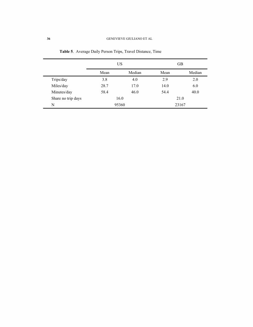
The results in this section are based on the full separate samples. Table 5 gives
average daily person trips, travel distance, and travel time. The basic measure of travel
– trips -- is much lower for GB. Not only do the British make fewer daily trips, they
are more likely to not have traveled at all on the survey day, despite the greater
attention paid in the NTS survey to very short trips. About one fifth of the British
sample did not travel on Day 7, compared to 16 percent for Americans. Note that if
there is any bias in the trip numbers, it is to underestimate short trips in the US sample.
Hence differences may be even larger than these numbers indicate.
On average, Americans travel twice as far as the British, but spend only a few
more minutes per day traveling. The relative consistency in time spent traveling is the
basis of travel budget theory: people have a fixed time budget for travel, and the cost
and speed of available modes determine number of trips and travel distance. In this
case, we might interpret the significantly lower British rate of travel a response to
limited transportation resources. As would be expected, US average trip length is
18 GENEVIEVE GIULIANO ET AL
much longer (7.5 miles vs 4.8 miles for GB), but average trip time is shorter (15.2
minutes vs 18.9 minutes for GB). See Figure 2.
Distribution of trips by purpose is also different. Work or work related trips
and personal business trips make up a larger share for Americans, while
social/recreational trips make up a smaller share, relative to the British. The greater
share of these trips in the GB sample may be due to more complete reporting of very
short walk trips.
Modal shares (based on total person trips) are given in Table 6. Differences are
dramatic. First, about 89 percent of all US person trips are made by privately owned
vehicle (POV), while the combined share of private vehicle trips for GB is about 58
percent. Second, within the POV category, the big difference is in driver trips.
Because of the way trips are recorded, there is no direct way to determine vehicle
occupancy (what may or may not be a multi-person trip). However, the share of driver
trips is an indicator of vehicle occupancy; obviously a much larger share of US trips is
drive alone trips. Second, the transit share is under 2 percent in the US, but around 8
percent for GB. Third, use of non-motorized modes is more than four times as
frequent in GB as in the US. Such trips account for about one third of all trips.
Recalling again the emphasis of the NTS on short trips, the non-motorized share for
US may be biased downward.
As has been noted in numerous studies (e.g. Dunn, 1981; Pucher, 1988; Orfeuil
and Salomon, 1993), a major explanatory factor for these differences is the difference
in the cost of owning and operating an automobile. The combined effects of the VAT
ANOTHER LOOK AT TRAVEL PATTERNS AND URBAN FORM 19
and sales tax add about 25 percent to the price of a new automobile in Great Britain,
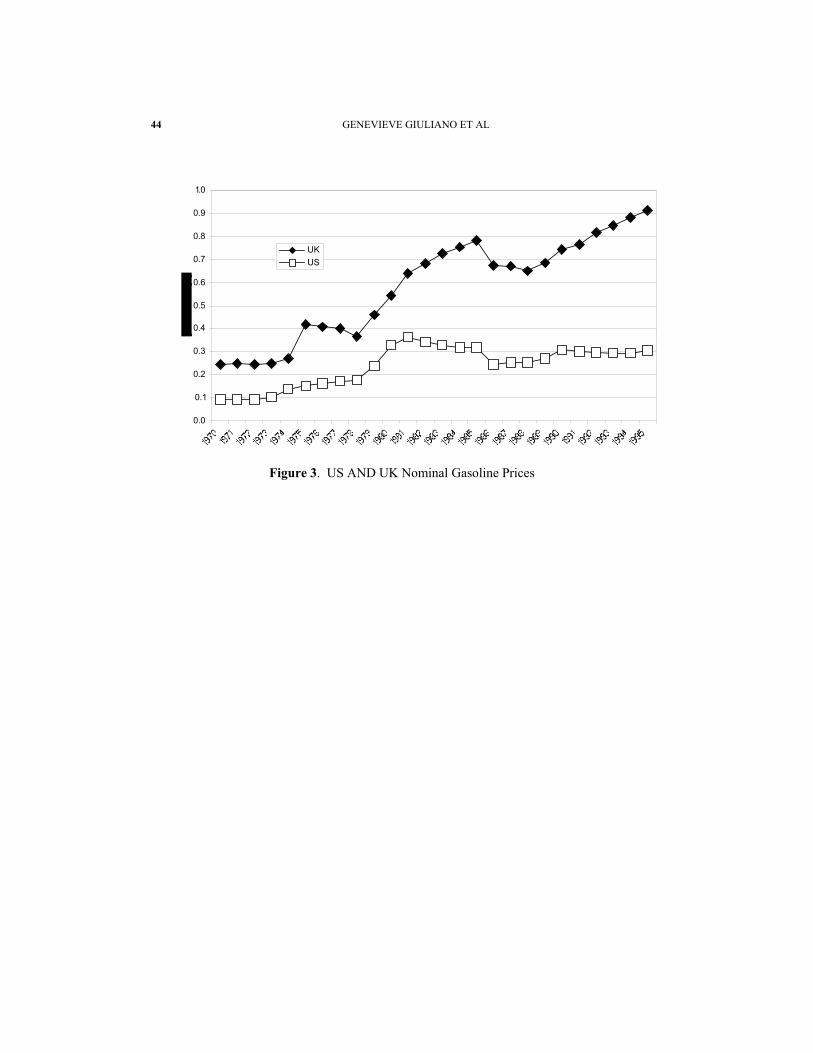
compared to sales taxes of 5 to 8 percent in the US. In 1999, the price of petrol and
diesel in Great Britain was the highest in the European Union, a result of the UK’s
unique fuel tax escalator (Mitchell and Lawson, 2000). Figure 3 gives per liter gasoline
costs by year for the US and UK, in ppp (purchase power parity) equivalents. The UK
price has risen from $ 0.25 per liter in 1970 to $ 0.90 per liter in 1995. Over the same
period the US price increased from $ 0.10 to $ 0.30. Thus the difference in gasoline
prices between these countries has quadrupled in the 25 year period.
Regression Model Results
We estimated two sets of regression models, one with trips as the dependent
variable, the other with distance, using the pooled sample. Our control variables
include sex, age, household income, and employment status. All are coded as
categorical dummy variables. Previous research indicates that this small set of control
variables is adequate. We use as a measure of car access the ratio of cars to drivers in
the individual’s household. Admittedly this measure has a US “bias”: we assume that
the car is the preferred mode, and when there are fewer cars than drivers, some
household members will choose other modes or will forego a trip. Under some
conditions, it is possible that the car is not the preferred mode.
Total Daily Trips
Starting with trips, Table 7 gives results for the full model, and Table 8 gives
results for the reduced form model. Coefficients and standard errors are given for the

20 GENEVIEVE GIULIANO ET AL
total sample in the first panel of numbers; the same data are given for the Great Britain
interaction terms in the second panel. We use a conservative measure of statistical
significance.8 The estimations were conducted using stepwise regression. The last
column gives the F-test significance level for each additional group of variables. Each
row of coefficients provides comparisons between the US and Great Britain, with
comparisons being relative to the US. The effect for British persons is the sum of the
values of the two coefficients. Because the independent variables are category
dummies, the relative magnitude of the coefficients may be directly interpreted.
Considering first the group of socio-economic characteristics, we find that sex
has no significant relationship with total daily trips. Children and older people make
fewer trips, as expected; income and employment effects are also as expected. Only
one of the interaction dummy variable coefficients is significant, meaning that overall,
these socio-economic factors work the same way in both countries (more precisely, we
cannot reject the null hypothesis that there are no differences between the two groups).
The one significant income interaction dummy coefficient suggests that for GB, trip
rates between the two middle income groups are more similar, and trip rates between
the third and highest groups are less similar than is the case for the US (recall that the
income groups are based on equivalent incomes).
We use as a measure of car access the ratio of cars to drivers in the individual’s
household. As expected, individuals with no car in the household have the lowest trip
8 The complex weighting procedure employed in the NPTS sample creates statistical difficulties in conducting inference tests. To minimize these problems, we use a stricter

ANOTHER LOOK AT TRAVEL PATTERNS AND URBAN FORM 21
rates relative to the omitted category (cars = drivers), and the effect is quite
pronounced. The effect of having fewer cars than drivers is also negative, but of much
smaller magnitude. Again, there is no difference in the effects of car access between
Great Britain and the US.
We use two measures of urban form, metropolitan location and population
density in the place of residence. We do not expect urban form measure to have much
influence on trip rates; influence should be greater on travel distance. Possibly trip
rates are lower in very inaccessible places and higher in very accessible places. Table
6 shows that the smaller MSAs are associated with more trip making relative to larger
MSAs. Residing in very high density areas is associated with less trip making relative
to lower density areas. In the US, this may be explained by the relatively high share of
low income households residing in high density areas, but this may not be the case for
Great Britain. Note that none of the interaction dummy variable coefficients are
significant, either individually or as a group, meaning that these measures of urban
form have no different relationship with trip making between the two countries.
Finally, the Great Britain dummy coefficient is significant and negative as
expected. The dummy captures the many differences between the two countries not
explicitly controlled for in the model. Given the much lower average trip rate of the
British sample, the value of the coefficient is somewhat low.
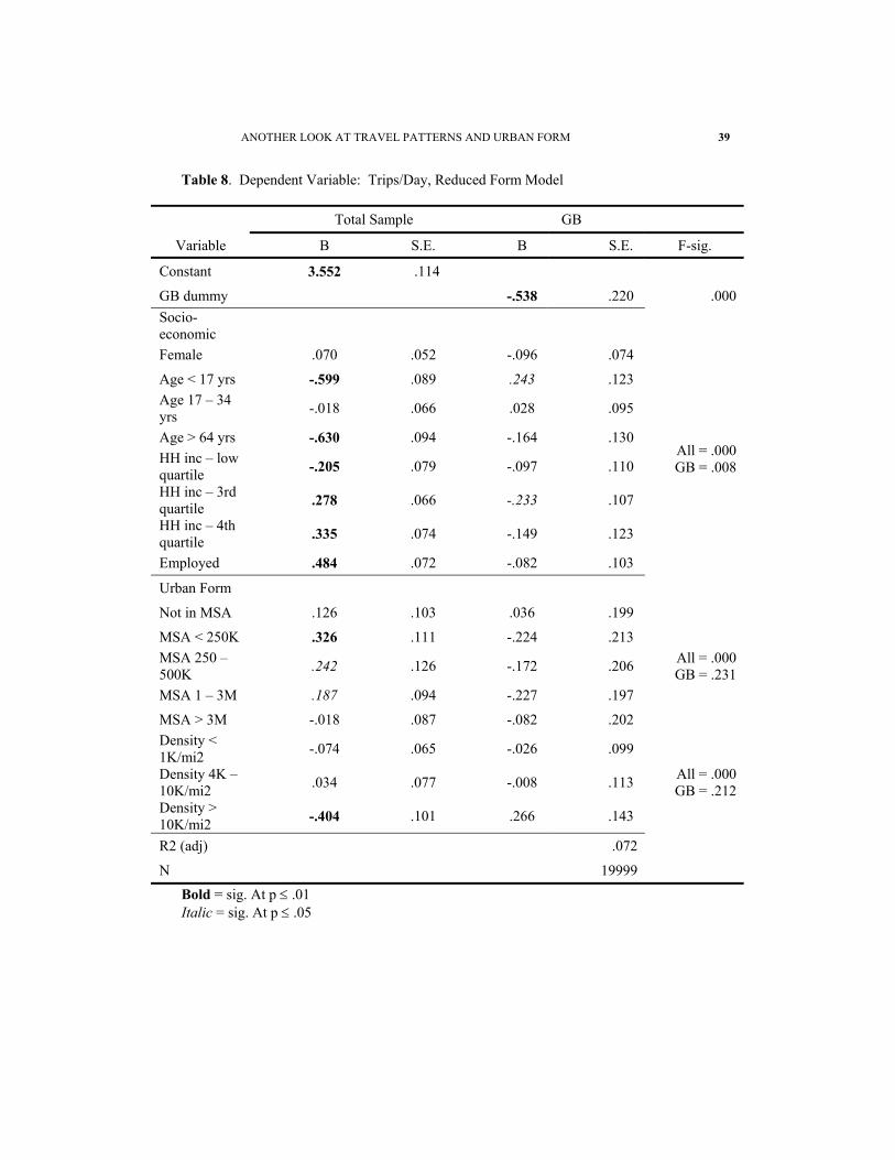
Table 8 gives results for the reduced form model. Results are quite similar.
The Great Britain dummy coefficient is greater in magnitude, as are the income and
significance level. See Giuliano (2002) for further discussion. See NPTS Users Guide,
22 GENEVIEVE GIULIANO ET AL
employment variable coefficients. This makes sense: the car ownership effects are
now captured by these variables. As before, there are few differences between the US
and British sample with respect to socio-economic variables. Results for the urban
form variables are quite similar to those for the full model, with the exception of high
density, which increases in magnitude. This may be due to correlation between
household income and density in the US data, as well as a “New York effect”, meaning
the relatively low rate of car ownership in the highest density areas.
We may summarize the results of the trip regressions as follows. First, the
models explain very little of the variation in trip making. Also, these models are quite
simple, while the differences between trips on various modes and for various purposes
are quite substantial. Second, basic socio-economic characteristics are important
explanatory factors and work the same way in both countries. Hence some of the
difference we observe between the US and Great Britain is due to lower household
income and different population demographics. Third, our urban form variables have
little effect on trip making for either group. The relationship between high density and
less trip making is a US phenomenon and may to be linked to the spatial distribution of
the low income population. Finally, the pooled model has about the same explanatory
power for both groups. Separate regressions yield a comparable R2 (results not
shown).
Appendix G on estimating sampling errors.
ANOTHER LOOK AT TRAVEL PATTERNS AND URBAN FORM 23
Total Daily Miles Traveled
Tables 9 and 10 give model results for total daily travel distance. Because the
distribution of the dependent variable is skewed towards long distances, we use the
natural log form.9 Starting with the full model (Table 8), the socio-economic variable
coefficients are mostly significant and of the expected sign (first panel). More miles
traveled is associated with male sex, adult age, higher household income, and being
employed. Only one of the interaction dummy coefficients is significant: third quartile
income. As with the trip results, this suggests more similarity between the two middle-
income groups for the British. The British dummy variable coefficient is of the
expected sign, but not significant. Given that the British on average travel half as
many daily miles as the Americans, this is somewhat surprising.
Greater car access is associated with more daily travel distance, as expected,
with the coefficient for no cars in the household of greatest negative magnitude.
Results for the interaction terms are interesting: the positive coefficient for cars less
than drivers is consistent with public transport playing a more important role in Great
Britain. The greater availability and higher quality of public transport in Great Britain
makes it a closer substitute to the car than in the US. When people have discretionary
income to spend on transportation, one can purchase more public transport and achieve
a relatively high level of mobility.
Turning to metropolitan size, none of the coefficients for the total sample are
significant, though there is a suggestion of a pattern of more daily miles in the larger

24 GENEVIEVE GIULIANO ET AL
MSAs. The interaction coefficients are all negative, and three are significant. It is
difficult to interpret these results, given the very different distributions of the two
groups across metropolitan size categories (see Table 3).
The most interesting results are those for residential density. Two of the three
coefficients for the total sample are significant and of the expected sign. However,
coefficients for the interaction variables are also significant and of the opposite sign.
The combined effect indicates that there is no relationship between daily travel
distance and density among the British. We would expect that given the higher relative
price of motorized travel, the British would be more inclined to economize and
therefore make shorter trips in more accessible places.10 There are two possible
explanations for these results. First, the greater availability and higher quality of
transit may provide a more uniform level of transport access across levels of density.
Second, mixed patterns of land use are widespread, and consequently population
density may be a less useful measure of urban form in Great Britain. That is, the
higher price of travel promotes economizing everywhere, and land use patterns make
such economizing possible. Recall that the British density measure is more aggregate
than that of the US, so very high or very low density is lost in the aggregation. Thus
our measure could have the effect of underestimating the relationship.
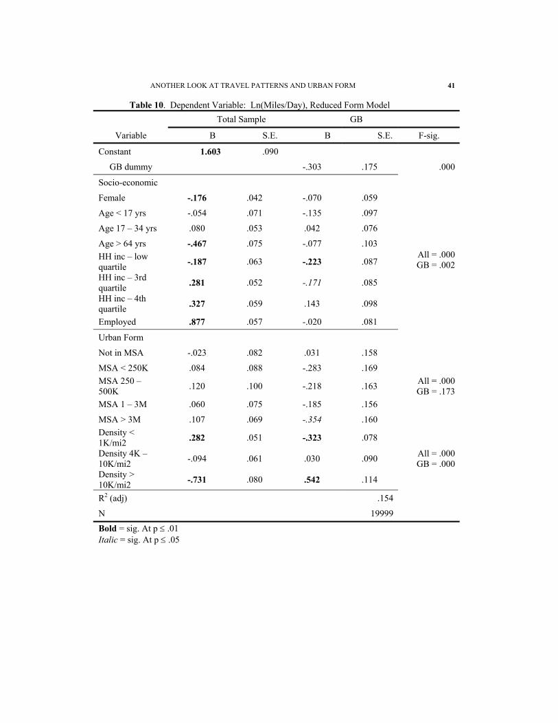
The reduced form results in Table 9 are similar to those of the full model. As
with the trip regressions, the income and employment coefficients are somewhat
9 Specifically, we use Ln(distance + 0.1) to retain persons with zero trips in the regression.
ANOTHER LOOK AT TRAVEL PATTERNS AND URBAN FORM 25
greater in magnitude. There is a more negative effect for the low-income interaction
term, likely reflecting the large proportion of no car households in this category. The
metropolitan size variable coefficients are largely unchanged; the high-density
coefficient becomes more negative, again reflecting the concentration of US low-
income households in the highest density areas.
6. Conclusions
We draw the following conclusions from our results. First, there are few differences in
the way that socio-economic and urban form characteristics are associated with travel
patterns between the US and Great Britain. With few exceptions, sex, age, household
income and employment status have similar effects. Therefore observed differences
between countries are in part explained by differences in population characteristics,
notably lower household income for the British.
Second, car access is a powerful explanatory force for both trip making and
travel distance. Individuals residing in households with no cars make significantly
fewer daily trips and travel significantly fewer miles, all else equal. We noted earlier
that car access might not work the same way in Great Britain, as we would expect
more households to choose not to own cars, given the greater availability of public
transit and high access neighborhoods. The reduced effect of fewer cars than drivers
(essentially one car households) for the British is consistent with this hypothesis.
10 Deregulation and privatization have resulted in relatively high fares for public transport, compared to typical US transit fares.

26 GENEVIEVE GIULIANO ET AL
When we remove the car access variables from the model, income and employment
effects increase in magnitude, as expected.
Third, metropolitan size has a small but significant relationship with trips, but
not with travel distance. It is difficult to explain the results for daily trips, since there
is no obvious reason why trip frequency should be a function of metropolitan size. It is
possible that more and shorter trips take place in smaller, more self-contained metro
areas. We expected more effects for travel distance. As we noted earlier, large MSAs
provide accessibility across large spatial areas, so there are relatively more
opportunities for longer distance trips. In addition average journey-to-work trip length
increases with metropolitan size.
Fourth, while residential density has the expected relationship with travel
distance for the US sample, there is no relationship between density and travel distance
for the British sample, once other relevant factors are controlled. We speculate that
this may reflect more use of transit in the highest density British areas, and may even
reflect something of a “London effect” – most of the highest density zones are in
Central London, where transit service is particularly extensive. The results may also
reflect the greater concentration of low-income households in high-density areas in the
US. In any case, these results lend little support to the idea that more compact urban
form leads to less travel distance. More research is certainly in order on this question.
Our literature review discussed various perspectives on the differences in travel
patterns between the US and Europe. One perspective emphasized policy differences,
which, together with historical development and technological change, have led to

ANOTHER LOOK AT TRAVEL PATTERNS AND URBAN FORM 27
more compact urban environments and higher costs for automobile use in Europe.
Another perspective emphasizes household income, arguing that auto ownership and
use is largely a function of per capita income. Our results tend to support the latter
perspective: socio-economic characteristics are significant and generally consistent
across the two countries. Results for our land use measures are more mixed.
Our research suffers from some obvious limitations. First, we have used just
two simple measures of urban form; ideally one would include a more direct measure
of accessibility, and better measures of metropolitan spatial structure. We are currently
in the process of developing better measures of urban form. It is also argued that the
spatial characteristics that matter are highly localized neighborhood characteristics, e.g.
local access to shops and services, pedestrian friendly streets. Hanson and Schwab’s
Swedish study (1987) shows the significance of local accessibility; later work by
others has yielded more mixed results (Boarnet and Crane, 2001). Unfortunately, data
limitations preclude such comparisons across the two countries.
Second, we have not directly incorporated prices or measures of transportation
supply (e.g. access to transit, road supply). Given a two-country comparison, price
effects are incorporated in the country dummy variable. However, transportation
supply must have significant within country variation (consider transit access in the
US), yet we have implicitly assumed within-country homogeneity. These supply
effects are incorporated in the country dummy variable (and to some extent in the
urban form measures) along with all the other unmeasured --many not measurable--
differences between the two countries. Third, some would argue that we are using

28 GENEVIEVE GIULIANO ET AL
measures of travel that are too aggregate. The choice process may be different across
trip purposes, for example. We argue that it is appropriate to use measures of total
mobility in this type of study, though there is much to be learned from more targeted
analysis. Finally, our reduced form model is a very basic way to address the
endogeneity problem; a two-stage approach allowing car ownership choice to be
modeled explicitly might yield better results. Despite these limitations, however, our
results provide a starting point for systematic comparative analysis of travel patterns
and urban form.
Acknowledgement
This research was supported by the General Motors Foundation, the USC School of Policy, Planning, and Development, and by the USC Lusk Center for Real Estate. Research assistance was provided by graduate students Dhiraj Narayan, His-Hwa Hu, and Hyung-Cheal Ryu. Lee Schipper, University of California, Berkeley, provided the NTS survey data and collaborated on development of the data sets and descriptive analysis of the data. Ms. Barbara Noble and Mr. Darren Williams, Department of Environment, Transport, and the Regions, UK, assisted with NTS data preparation. Comments from participants at the ITS Seminar (Berkeley, CA, September 2001), the STELLA Focus Group 5 meeting (Brussels, April 2002), Joyce Dargay and Peter Gordon are greatly appreciated. All errors and omissions are the responsibility of the authors.
ANOTHER LOOK AT TRAVEL PATTERNS AND URBAN FORM 29
References
BERNICK, M. and R. CERVERO (1997) Transit Villages in the 21st Century, McGraw-Hill, New
York.
BOARNET, M. and R. CRANE. (2001) Travel by Design. New York: Oxford University Press.
CERVERO, R. (1995) “Planned communities, self-containment and commuting: A cross-
national perspective, Urban Studies, Vol. 32, No. 7, 1135-1161.
CHINITZ, B. (1991) “A framework for speculating about future urban growth patterns in the
U.S., “Urban Studies, 28(6), 939-959.
CLARK, W.A.V. and M. KUPERS-LINDE (1994) Commuting in restructuring Urban regions,
Urban Studies V31-3 p465-84.
DARGAY, J and D. GATELY, (1997), “Income’s Effect on Car and Vehicle ownership,
Worldwide: 1960-2015” Transportation Research 33A(7/8), 101-138.
DUNN, J (1981) Miles to go: European and American Transportation policies. MIT press:
Cambridge, MA.
GILLESPIE, A. (1999) “The changing employment geography of Britain,” in M Breheny (ed)
The People: Where Will They Work?, Town and Country Planning Association, London.
GIULIANO, G. (2002) “Travel, location and race/ethnicity,” Transportation Research A,
forthcoming.
GIULIANO G., H-H HU and D. NARAYAN (2000) “International Travel Project” Working Paper
1. Unpublished; available from the author. University of Southern California, Los Angeles.
GIULIANO, G. (1999) “Land use and transportation: Why we won’t get there from here,”
Transportation Research Circular, 492, 179-198.
GOMEZ-IBANEZ, J. A. (1991) "The Political Economy of Highway Tolls and Congestion
Pricing" Paper presented at the Seminar on the Application of Pricing Principles to
Congestion Management, Federal Highway Administration, Washington, D.C.

30 GENEVIEVE GIULIANO ET AL
GORDON, P. and H.W. RICHARDSON (1989) Gasoline Consumption and Cities - A Reply.
Journal of the American Planning Association, 55, 342-346.
HANSEN, G.R.M (1993) Commuting: Home sprawl, job sprawl, traffic jams. In A Billion Trips
a Day: Tradition and Transition in European Travel Patterns, eds. I. Salomon, P. Bovy and
J.P. Orfeuil. Kluwer Academic Publishers, Dordrecht, The Netherlands, 101-127.
HANSON, S. and M. SCHWAB. (1987) “Accessibility and Intraurban Travel.” Environment and
Planning A, 19: 735-748.
INGRAM, G.K. and Z. LIU (1999) “Determinants of Motorization and Road provision” in Essays
in Transportation Economics and Policy. Brookings Institution Press, Washington.
JACKSON, K. (1985) The Crabgrass Frontier. Oxford University Press, New York.
KASARDA, J. (1995) “Industrial restructuring and the challenging location of jobs”. In State of
the Union, ed. R. Farley. Russel Sage Foundation, New York.
KUTAY,A. (1988a) Technological change and spatial transformation in an information
economy:1. A structural model of transition in the urban system. Environment and Planning
A 20. 569-593.
KUTAY,A. (1988b) Technological change and spatial transformation in an information
economy:2. The influence of new information technology on the urban system. Environment
and Planning A 20. 707-718.
LAVE, C. (1996) Are Americans really driving so much? Access 8, 14-17.
MEYER, J AND J.A.GOMEZ-IBANEZ (1981) Auto Transit and cities. A twentieth century fund
report. Harvard University Press: Cambridge, MA.
MITCHELL, C. AND S. LAWSON (2000) The Great British Motorist 2000.
MULLER, P. (1981) Contemporary Suburban America. Englewood Cliffs, NJ: Prentice-Hall.
NEWMAN, P. and J. KENWORTHY (1998) Sustainability and Cities: Overcoming Automobile
Dependence. Washington, DC: Island Press.

ANOTHER LOOK AT TRAVEL PATTERNS AND URBAN FORM 31
NEWMAN, P. and J. KENWORTHY (1989a) “Gasoline consumption and cities”. Journal of the
American Planning Association Winter: 24-37.
NEWMAN, P. and J. KENWORTHY (1989b) Cities and Automobile Dependence: An International
Sourcebook. Brooksfield Vt: Gower Technical.
NIEMEIER, D. and RUTHERFORD (1994). Non-Motorized Transportation, NPTS: Travel Mode
Special Reports, U.S. Department of Transportation, Federal Highway Administration,
Office of Highway Information Management, Washington, D.C.
NIVOLA, P. S. (1999) Laws of the Landscape: How Policies Shape Cities in Europe and
America Washington, DC: Brookings Institution Press Washington.
ORFEUIL, J.P. and I. SALOMON (1993) “Travel Patterns of the Europeans in every day life”. In A
billion Trips a Day: Tradition and transition in European Travel Patterns, eds. I. Salomon,
P. Bovy and J.P. Orfeuil. Kluwer Academic Publishers, Dordrecht, The Netherlands.
PUCHER JOHN and C. LEFEVRE. (1996) The Urban Transport Crisis – in Europe and North
America. Great Britain: McMillan Press Ltd.
PUCHER, JOHN (1988) Urban Travel Behavior as the outcome of public policy. Journal of the
American Planning Association 54(3), 509-519.
PUSHKAREV, B. and J. ZUPAN (1977) Public Transportation and Land Use Policy.
Bloomington: Indiana University Press.
SCHAFER, A. and D. G. VICTOR (1997) “The Future Mobility of the World Population”.
Discussion Paper 97-6-4, Massachusetts Institute of Technology, Center for Technology,
Policy, and Industrial Development, Cambridge, MA.
SCHIMEK, PAUL. (1996). "Household Motor Vehicle Ownership and Use: How Much Does
Residential Density Matter?" Transportation Research Record 1552: 120-25.
ZAHAVI Y, and A. TALVITIE (1980). Regularities in travel time and money expenditures,
Transportation Research Record 750: 13-19.
32 GENEVIEVE GIULIANO ET AL
Table 1. Basic Statistics, US And UK
US UK
Population (2000 est.) 275,500,000 59,500,000 Land Area (km2) 9,158,960 241,590 Median Household Income (ppp, 1999) $33,900 $21,800
List of Tables
ANOTHER LOOK AT TRAVEL PATTERNS AND URBAN FORM 33
Table 2. Basic Sample Characteristics
NPTS NTS
Total households 42,033 9,688 Total persons 95,360 23,167 Total trips 409,025 377,560a a Full seven-day file

34 GENEVIEVE GIULIANO ET AL
Table 3. Place of residence metropolitan area size, share of persons, percent
NPTS 1995 NTS 1995
Not in MSA 14.4 40.6
100K - 250K 9.6 9.1
250K – 500K 6.4 24.8
500K – 1 M 12.7 3.0
1 M – 3 M 18.8 10.7
> 3 M 38.1 11.5

ANOTHER LOOK AT TRAVEL PATTERNS AND URBAN FORM 35
Table 4. Car Access, persons
NPTS 1995 NTS 1995
No car in HH 3.0 23.2
Cars < drivers 17.0 25.8
Cars = drivers 64.0 48.0
Cars > drivers 16.0 3.0
36 GENEVIEVE GIULIANO ET AL
Table 5. Average Daily Person Trips, Travel Distance, Time
US GB
Mean Median Mean Median
Trips/day 3.8 4.0 2.9 2.0 Miles/day 28.7 17.0 14.0 6.0 Minutes/day 58.4 46.0 54.4 40.0 Share no trip days 16.0 21.0 N 95360 23167

ANOTHER LOOK AT TRAVEL PATTERNS AND URBAN FORM 37
Table 6. Modal shares
US GB
POV driver 63.1 37.1
POV passenger 26.1 21.1
Bus 1.2 6.6
Rail 0.5 1.6
Bike/walk 6.8 32.3
Other 2.3 1.3
N 395157 66737

38 GENEVIEVE GIULIANO ET AL
Table 7. Dependent variable: trips/day, full model Total Sample GB
Variable B S.E. B S.E. F-sig.
Constant 3.619 .116
GB dummy -.432 .223 .000
Socio-economic
Female 0.069 .052 -.076 .074
Age < 17 yrs -0.602 .092 .230 .122
Age 17 – 34 yrs -0.009 .066 .046 .095
Age > 64 yrs -0.640 .094 -.111 .130 HH inc – low quartile -0.158 .079 .005 .112
HH inc – 3rd quartile 0.258 .066 -.225 .107
HH inc – 4th quartile 0.312 .074 -.140 .123
Employed 0.473 .072 -.127 .103
All = .000 GB =.008
Cars
No car HH -0.728 .162 .174 .178
Cars < drivers -0.198 .068 .149 .093 Cars > drivers -0.039 .076 -.246 .172
All = .000 GB = .020
Urban Form
Not in MSA 0.126 .103 -.061 .199
MSA < 250K 0.329 .111 -.302 .212
MSA 250 – 500K 0.242 .125 -.261 .206
MSA 1 – 3M 0.177 .094 -.297 .197
MSA > 3M -0.012 .086 -.145 .201
Density < 1K/mi2 -0.086 .065 -.036 .099 Density 4K – 10K/mi2 0.047 .077 -.018 .113
Density > 10K/mi2 -0.286 .103 .187 .145
All = .003 GB = .484
R2 (adj) .076
N 19999
Bold = sig. At p ≤ .01 Italic = sig. At p ≤ .05
ANOTHER LOOK AT TRAVEL PATTERNS AND URBAN FORM 39
Table 8. Dependent Variable: Trips/Day, Reduced Form Model
Total Sample GB
Variable B S.E. B S.E. F-sig.
Constant 3.552 .114
GB dummy -.538 .220 .000 Socio-economic
Female .070 .052 -.096 .074
Age < 17 yrs -.599 .089 .243 .123 Age 17 – 34 yrs -.018 .066 .028 .095
Age > 64 yrs -.630 .094 -.164 .130 HH inc – low quartile -.205 .079 -.097 .110
HH inc – 3rd quartile .278 .066 -.233 .107
HH inc – 4th quartile .335 .074 -.149 .123
Employed .484 .072 -.082 .103
All = .000 GB = .008
Urban Form
Not in MSA .126 .103 .036 .199
MSA < 250K .326 .111 -.224 .213 MSA 250 – 500K .242 .126 -.172 .206
MSA 1 – 3M .187 .094 -.227 .197
MSA > 3M -.018 .087 -.082 .202
All = .000 GB = .231
Density < 1K/mi2 -.074 .065 -.026 .099
Density 4K – 10K/mi2 .034 .077 -.008 .113
Density > 10K/mi2 -.404 .101 .266 .143
All = .000 GB = .212
R2 (adj) .072
N 19999
Bold = sig. At p ≤ .01 Italic = sig. At p ≤ .05

40 GENEVIEVE GIULIANO ET AL Table 9. Dependent Variable: Ln(Miles/Day), Full Model
Total Sample GB
Variable B S.E. B S.E. F-sig.
Constant 1.700 .091
GB dummy -.143 .176 .000
Socio-economic
Female -.177 .041 -.040 .058
Age < 17 yrs -.059 .070 -.154 .097
Age 17 – 34 yrs -.092 .052 .071 .075
Age > 64 yrs -.475 .074 -.002 .103 HH inc – low quartile -.129 .063 -.055 .088
HH inc – 3rd quartile .254 .052 -.162 .084
HH inc – 4th quartile .292 .059 .150 .097
Employed .862 .057 -.089 .081
All = .000 GB = .002
Cars
No car HH -.782 .128 -.051 .141
Cars < drivers -.334 .054 .248 .073 Cars > drivers -. 047 .060 -.191 .136
All = .000 GB = .000
Urban Form
Not in MSA -.024 .081 -.117 .158
MSA < 250K .093 .088 -.403 .168 MSA 250 – 500K .122 .099 -.351 .162
MSA 1 – 3M .049 .074 -.292 .155
MSA > 3M .118 .068 -.446 .159
All = .001 GB = .072
Density < 1K/mi2 .267 .051 -.342 .078
Density 4K – 10K/mi2 -.075 .061 .015 .089
Density > 10K/mi2 -.586 .082 .453 .115
All = .000 GB = .000
R2 (adj) .167
N 19999
Bold = sig. At p ≤ .01 Italic = sig. At p ≤ .05
ANOTHER LOOK AT TRAVEL PATTERNS AND URBAN FORM 41
Table 10. Dependent Variable: Ln(Miles/Day), Reduced Form Model Total Sample GB
Variable B S.E. B S.E. F-sig.
Constant 1.603 .090
GB dummy -.303 .175 .000
Socio-economic
Female -.176 .042 -.070 .059
Age < 17 yrs -.054 .071 -.135 .097
Age 17 – 34 yrs .080 .053 .042 .076
Age > 64 yrs -.467 .075 -.077 .103 HH inc – low quartile -.187 .063 -.223 .087
HH inc – 3rd quartile .281 .052 -.171 .085
HH inc – 4th quartile .327 .059 .143 .098
Employed .877 .057 -.020 .081
All = .000 GB = .002
Urban Form
Not in MSA -.023 .082 .031 .158
MSA < 250K .084 .088 -.283 .169 MSA 250 – 500K .120 .100 -.218 .163
MSA 1 – 3M .060 .075 -.185 .156
MSA > 3M .107 .069 -.354 .160
All = .000 GB = .173
Density < 1K/mi2 .282 .051 -.323 .078
Density 4K – 10K/mi2 -.094 .061 .030 .090
Density > 10K/mi2 -.731 .080 .542 .114
All = .000 GB = .000
R2 (adj) .154
N 19999
Bold = sig. At p ≤ .01 Italic = sig. At p ≤ .05

42 GENEVIEVE GIULIANO ET AL
List of Figures
40.7
28.7
20.9
9.8
34.1
27.7
20.5
17.7
0
5
10
15
20
25
30
35
40
45
Low (< 1000/sqmi) Medium (1K-4K/sqmi) High (4K-10K/sqmi) Very high (> 10K/sqmi)
With
in c
ount
ry p
erce
nt
US
GB
Figure 1. Population Density In Place Of Residence

ANOTHER LOOK AT TRAVEL PATTERNS AND URBAN FORM 43
0 5 10 15 20 25 30
GBUS
Trip Time (minutes)
Trip Distance (miles)
Trip Speed (mi/hr)
Figure 2. Average Trip Time, Length And Speed
44 GENEVIEVE GIULIANO ET AL
0.0
0.1
0.2
0.3
0.4
0.5
0.6
0.7
0.8
0.9
1.0
UKUS
Figure 3. US AND UK Nominal Gasoline Prices