anova: graphical. cereal example: nknw677.sas y = number of cases of cereal sold (cases) x = design...

ANOVA: Graphical

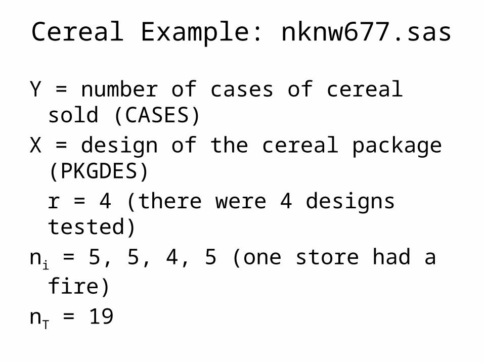
Cereal Example: nknw677.sas

Y = number of cases of cereal sold (CASES)X = design of the cereal package (PKGDES)

r = 4 (there were 4 designs tested)ni = 5, 5, 4, 5 (one store had a fire)

nT = 19

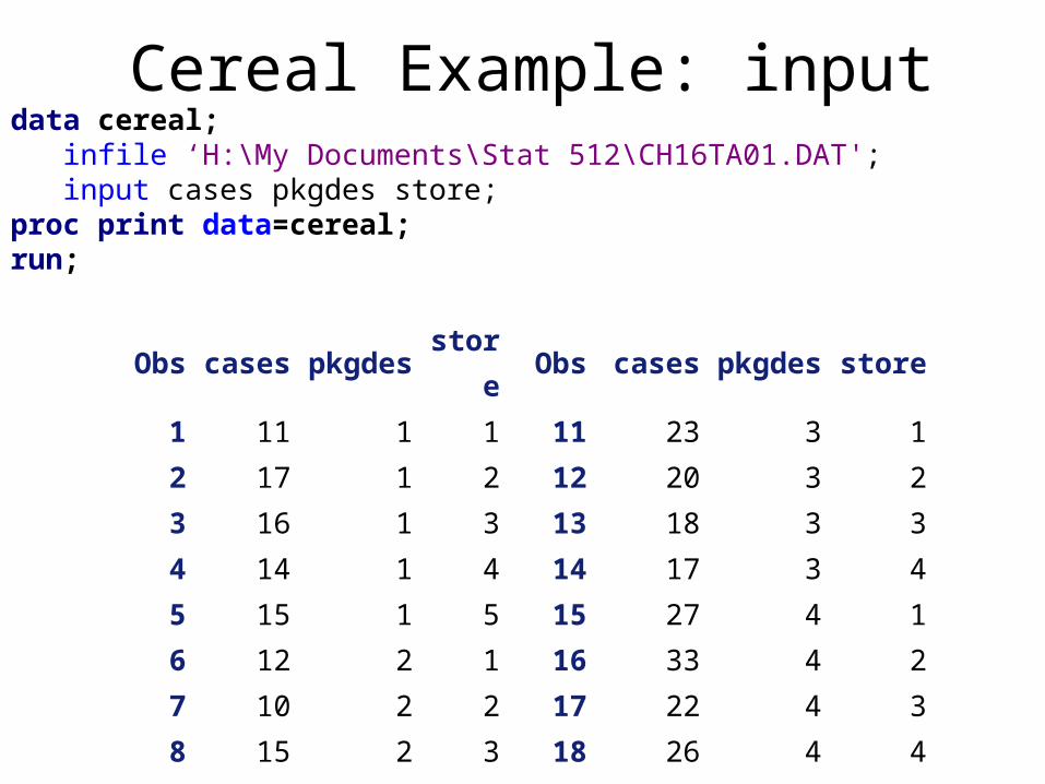
Cereal Example: inputdata cereal; infile ‘H:\My Documents\Stat 512\CH16TA01.DAT'; input cases pkgdes store;proc print data=cereal; run;

Obs cases pkgdes store Obs cases pkgdes store

1 11 1 1 11 23 3 12 17 1 2 12 20 3 23 16 1 3 13 18 3 34 14 1 4 14 17 3 45 15 1 5 15 27 4 16 12 2 1 16 33 4 27 10 2 2 17 22 4 38 15 2 3 18 26 4 49 19 2 4 19 28 4 5

10 11 2 5

Cereal Example: Scatterplottitle1 h=3 'Types of packaging of Cereal';title2 h=2 'Scatterplot';axis1 label=(h=2);axis2 label=(h=2 angle=90);symbol1 v=circle i=none c=purple;proc gplot data=cereal; plot cases*pkgdes /haxis=axis1 vaxis=axis2;run;

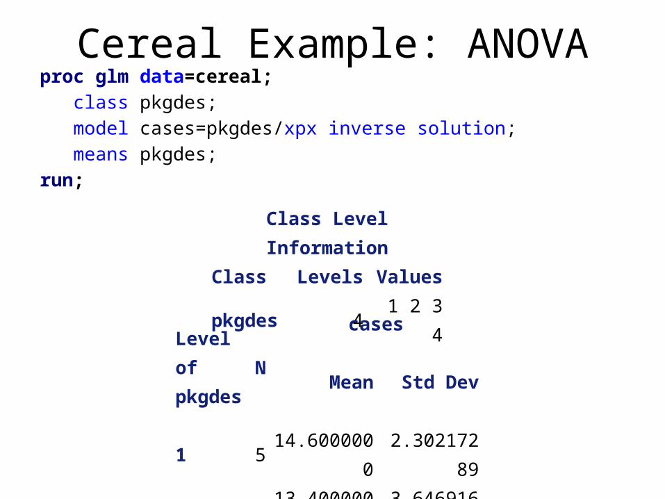
Cereal Example: ANOVAproc glm data=cereal; class pkgdes; model cases=pkgdes/xpx inverse solution; means pkgdes;run;

Class Level InformationClass Levels Valuespkgdes 4 1 2 3 4

Level ofpkgdes

Ncases

Mean Std Dev

1 5 14.6000000 2.30217289

2 5 13.4000000 3.64691651

3 4 19.5000000 2.64575131

4 5 27.2000000 3.96232255

Cereal Example: Meansproc means data=cereal; var cases; by pkgdes; output out=cerealmeans mean=avcases;proc print data=cerealmeans; run;

title2 h=2 'plot of means';symbol1 v=circle i=join;proc gplot data=cerealmeans; plot avcases*pkgdes/haxis=axis1 vaxis=axis2;run;

Types of packaging of Cerealplot of means

Obs pkgdes _TYPE_ _FREQ_ avcases1 1 0 5 14.62 2 0 5 13.43 3 0 4 19.54 4 0 5 27.2

Cereal Example: Means (cont)

ANOVA Table

Source of Variation df SS MS

Model(Regression) r – 1

Error nT – r

Total nT – 1

M

SSM

df

E

SSE

df

2i i. ..

i

n (Y Y )2

ij i.i j

(Y Y )2

ij ..i j

(Y Y )

ANOVA test

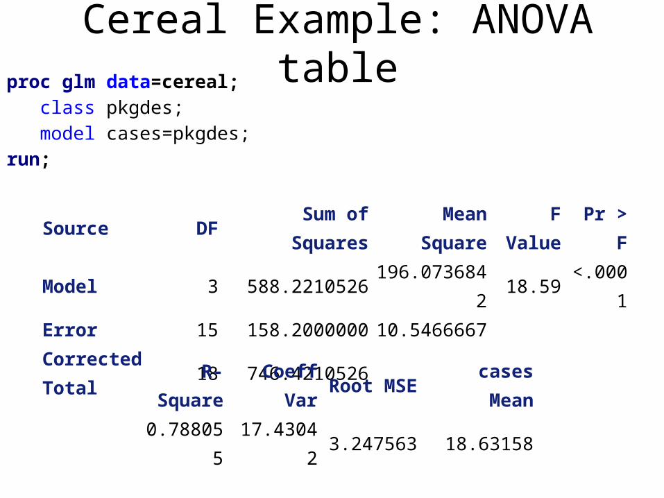
Cereal Example: ANOVA tableproc glm data=cereal; class pkgdes; model cases=pkgdes;run;

Source DF Sum of SquaresMean

SquareF Value Pr > F

Model 3 588.2210526 196.0736842 18.59 <.0001Error 15 158.2000000 10.5466667Corrected Total 18 746.4210526

R-Square Coeff Var Root MSE cases Mean0.788055 17.43042 3.247563 18.63158

Cereal Example:

Design Matrix

1 1 0 0 0

1 1 0 0 0

1 1 0 0 0

1 1 0 0 0

1 1 0 0 0

1 0 1 0 0

1 0 0 1 0

1 0 0 0 1

1 0 0 0 1

Cereal Example: Inverseproc glm data=cereal; class pkgdes; model cases=pkgdes/ xpx inverse solution; means pkgdes;run;

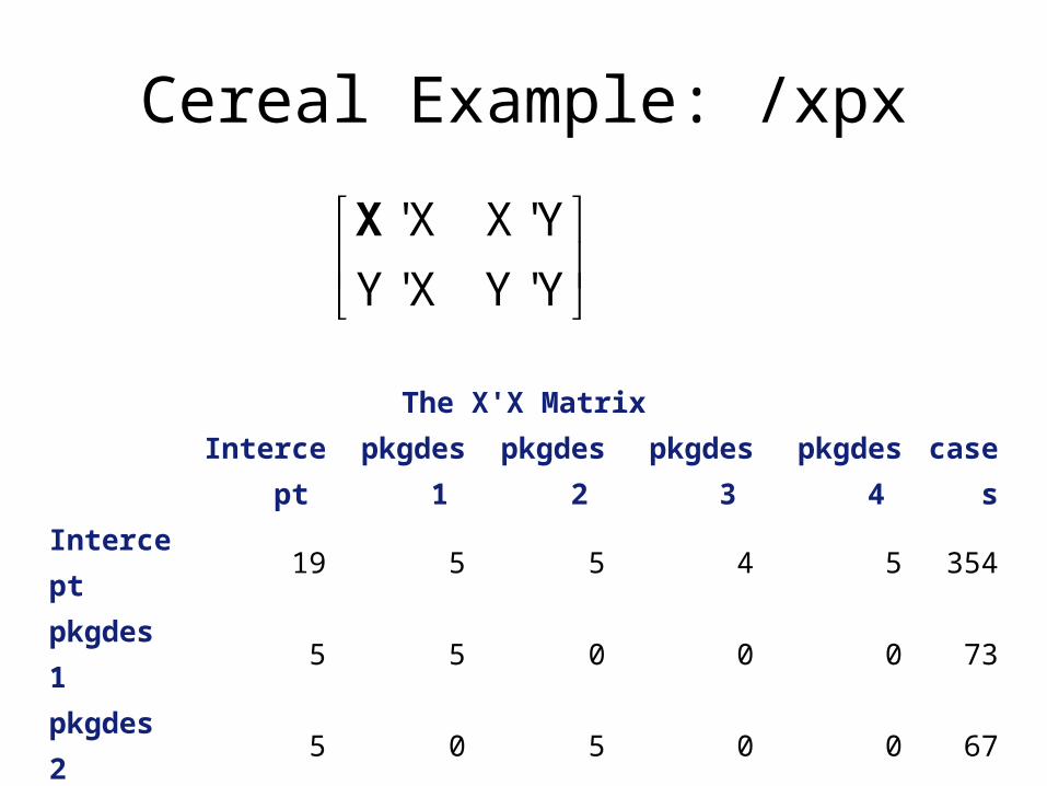
Cereal Example: /xpx

' X X'Y

Y ' X Y 'Y

X

The X'X MatrixIntercept pkgdes 1 pkgdes 2 pkgdes 3 pkgdes 4 cases

Intercept 19 5 5 4 5 354pkgdes 1 5 5 0 0 0 73pkgdes 2 5 0 5 0 0 67pkgdes 3 4 0 0 4 0 78pkgdes 4 5 0 0 0 5 136cases 354 73 67 78 136 7342

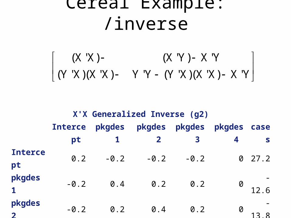
Cereal Example: /inverse

(X' X) (X'Y) X'Y

(Y ' X)(X' X) Y 'Y (Y ' X)(X' X) X'Y

X'X Generalized Inverse (g2)Intercept pkgdes 1 pkgdes 2 pkgdes 3 pkgdes 4 cases

Intercept 0.2 -0.2 -0.2 -0.2 0 27.2pkgdes 1 -0.2 0.4 0.2 0.2 0 -12.6pkgdes 2 -0.2 0.2 0.4 0.2 0 -13.8pkgdes 3 -0.2 0.2 0.2 0.45 0 -7.7pkgdes 4 0 0 0 0 0 0cases 27.2 -12.6 -13.8 -7.7 0 158.2

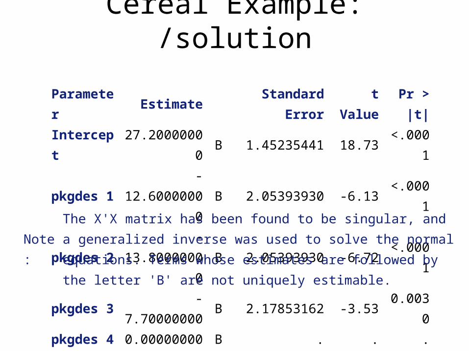
Cereal Example: /solution

Parameter Estimate Standard Error t Value Pr > |t|Intercept 27.20000000 B 1.45235441 18.73 <.0001pkgdes 1 -12.60000000 B 2.05393930 -6.13 <.0001pkgdes 2 -13.80000000 B 2.05393930 -6.72 <.0001pkgdes 3 -7.70000000 B 2.17853162 -3.53 0.0030pkgdes 4 0.00000000 B . . .

Note:The X'X matrix has been found to be singular, and a generalized inverse was used to solve the normal equations. Terms whose estimates are followed by the letter 'B' are not uniquely estimable.

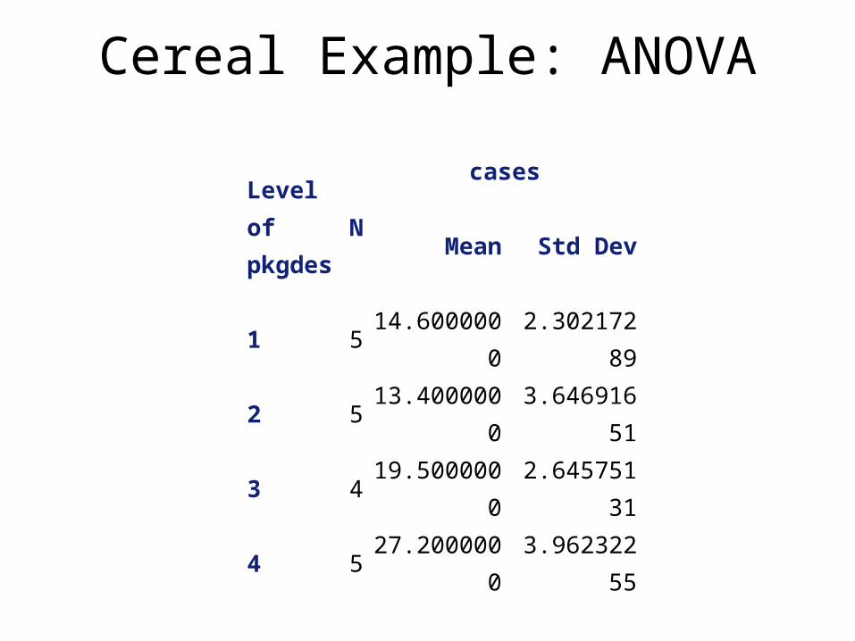
Cereal Example: ANOVA

Level ofpkgdes

Ncases

Mean Std Dev

1 5 14.6000000 2.30217289

2 5 13.4000000 3.64691651

3 4 19.5000000 2.64575131

4 5 27.2000000 3.96232255

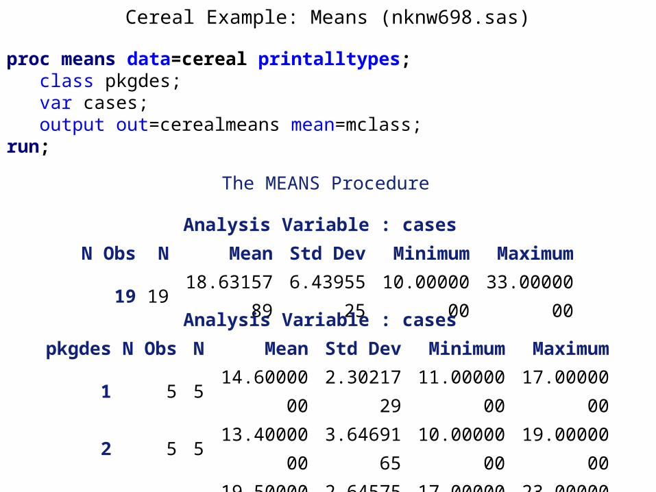
Cereal Example: Means (nknw698.sas)

proc means data=cereal printalltypes; class pkgdes; var cases; output out=cerealmeans mean=mclass; run;

Analysis Variable : cases N Obs N Mean Std Dev Minimum Maximum

19 19 18.63157896.439552

510.0000000 33.0000000

Analysis Variable : cases pkgdes N Obs N Mean Std Dev Minimum Maximum

1 5 5 14.60000002.302172

911.0000000 17.0000000

2 5 5 13.40000003.646916

510.0000000 19.0000000

3 4 4 19.50000002.645751

317.0000000 23.0000000

4 5 5 27.20000003.962322

622.0000000 33.0000000

The MEANS Procedure

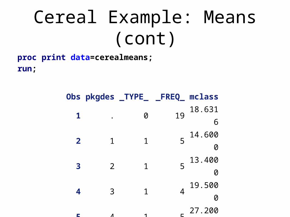
Cereal Example: Means (cont)proc print data=cerealmeans; run;

Obs pkgdes _TYPE_ _FREQ_ mclass1 . 0 19 18.63162 1 1 5 14.60003 2 1 5 13.40004 3 1 4 19.50005 4 1 5 27.2000

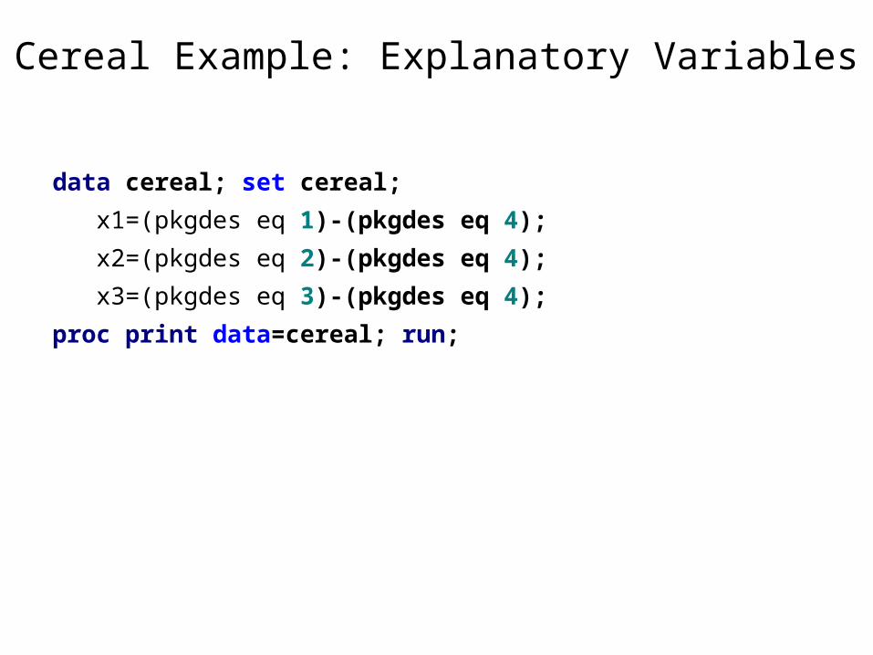
Cereal Example: Explanatory Variables

data cereal; set cereal; x1=(pkgdes eq 1)-(pkgdes eq 4); x2=(pkgdes eq 2)-(pkgdes eq 4); x3=(pkgdes eq 3)-(pkgdes eq 4);proc print data=cereal; run;

Cereal Example: Explanatory Variables (cont)Obs cases pkgdes store x1 x2 x3

1 11 1 1 1 0 02 17 1 2 1 0 03 16 1 3 1 0 04 14 1 4 1 0 05 15 1 5 1 0 06 12 2 1 0 1 07 10 2 2 0 1 08 15 2 3 0 1 09 19 2 4 0 1 0

10 11 2 5 0 1 011 23 3 1 0 0 112 20 3 2 0 0 113 18 3 3 0 0 114 17 3 4 0 0 115 27 4 1 -1 -1 -116 33 4 2 -1 -1 -117 22 4 3 -1 -1 -118 26 4 4 -1 -1 -119 28 4 5 -1 -1 -1

Cereal Example: Regression

proc reg data=cereal; model cases=x1 x2 x3;run;

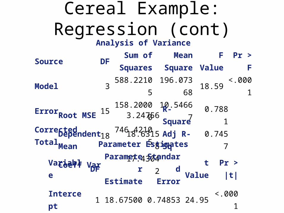
Cereal Example: Regression (cont)Analysis of Variance

Source DFSum of

SquaresMean


Model 3 588.22105196.0736

818.59 <.0001

Error 15 158.20000 10.54667Corrected Total 18 746.42105

Root MSE 3.24756 R-Square 0.7881Dependent Mean 18.63158 Adj R-Sq 0.7457Coeff Var 17.43042

Parameter Estimates

Variable DFParameter

EstimateStandard

Errort

ValuePr > |t|

Intercept 1 18.67500 0.74853 24.95 <.0001x1 1 -4.07500 1.27081 -3.21 0.0059x2 1 -5.27500 1.27081 -4.15 0.0009x3 1 0.82500 1.37063 0.60 0.5562

Cereal Example: ANOVAproc glm data=cereal; class pkgdes; model cases=pkgdes;run;

Source DFSum of

SquaresMean



R-Square Coeff Var Root MSEcases Mean

0.788055 17.43042 3.247563 18.63158

Cereal Example: ComparisonRegression

ANOVA

Analysis of Variance

Source DFSum of

SquaresMean


Model 3 588.22105196.0736

818.59 <.0001

Error 15 158.20000 10.54667Corrected Total 18 746.42105Root MSE 3.24756 R-Square 0.7881Dependent Mean 18.63158 Adj R-Sq 0.7457Coeff Var 17.43042

Source DFSum of

SquaresMean



R-Square Coeff Var Root MSEcases Mean

0.788055 17.43042 3.247563 18.63158

Cereal Example: Regression (cont)Analysis of Variance

Source DFSum of

SquaresMean


Model 3 588.22105196.0736

818.59 <.0001

Error 15 158.20000 10.54667Corrected Total 18 746.42105

Root MSE 3.24756 R-Square 0.7881Dependent Mean 18.63158 Adj R-Sq 0.7457Coeff Var 17.43042

Parameter Estimates

Variable DFParameter

EstimateStandard

Errort

ValuePr > |t|

Intercept 1 18.67500 0.74853 24.95 <.0001x1 1 -4.07500 1.27081 -3.21 0.0059x2 1 -5.27500 1.27081 -4.15 0.0009x3 1 0.82500 1.37063 0.60 0.5562

Cereal Example: Meansproc means data=cereal printalltypes; class pkgdes; var cases; output out=cerealmeans mean=mclass; run;

Analysis Variable : cases N Obs N Mean Std Dev Minimum Maximum

19 19 18.63157896.439552

510.0000000 33.0000000

Analysis Variable : cases pkgdes N Obs N Mean Std Dev Minimum Maximum

1 5 5 14.60000002.302172

911.0000000 17.0000000

2 5 5 13.40000003.646916

510.0000000 19.0000000

3 4 4 19.50000002.645751

317.0000000 23.0000000

4 5 5 27.20000003.962322

622.0000000 33.0000000

The MEANS Procedure

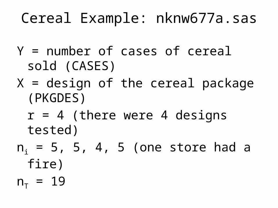
Cereal Example: nknw677a.sas

Y = number of cases of cereal sold (CASES)X = design of the cereal package (PKGDES)

r = 4 (there were 4 designs tested)ni = 5, 5, 4, 5 (one store had a fire)

nT = 19

Cereal Example: Plotting Meanstitle1 h=3 'Types of packaging of Cereal';proc glm data=cereal; class pkgdes; model cases=pkgdes; output out=cerealmeans p=means;run;

title2 h=2 'plot of means';axis1 label=(h=2);axis2 label=(h=2 angle=90);symbol1 v=circle i=none c=blue;symbol2 v=none i=join c=red;proc gplot data=cerealmeans; plot cases*pkgdes means*pkgdes/overlay

haxis=axis1 vaxis=axis2;run;

Cereal Example: Means (cont)

Cereal Example: CI (1) (nknw711.sas)proc means data=cereal mean std stderr clm maxdec=2; class pkgdes; var cases;run;

The MEANS Procedure

Analysis Variable : cases

pkgdes N Obs Mean Std Dev Std ErrorLower 95%

CL for MeanUpper 95%

CL for Mean

1 5 14.60 2.30 1.03 11.74 17.462 5 13.40 3.65 1.63 8.87 17.933 4 19.50 2.65 1.32 15.29 23.714 5 27.20 3.96 1.77 22.28 32.12

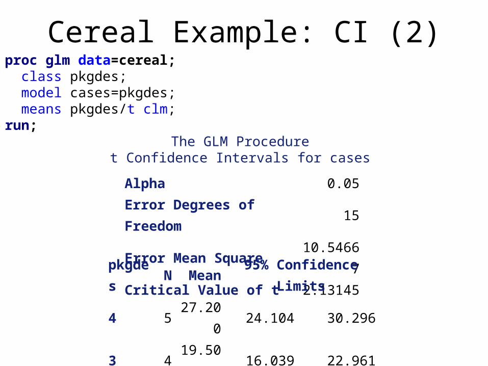
Cereal Example: CI (2)proc glm data=cereal; class pkgdes; model cases=pkgdes; means pkgdes/t clm;run;

The GLM Procedure t Confidence Intervals for cases

Alpha 0.05Error Degrees of Freedom 15Error Mean Square 10.54667Critical Value of t 2.13145

pkgdes N Mean 95% Confidence Limits4 5 27.200 24.104 30.2963 4 19.500 16.039 22.9611 5 14.600 11.504 17.6962 5 13.400 10.304 16.496

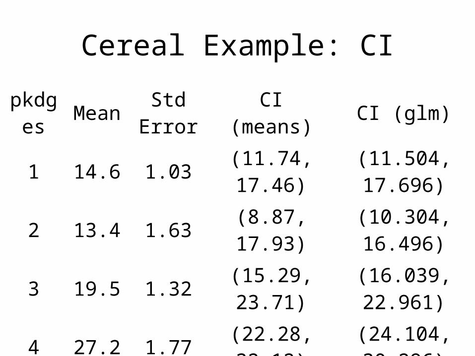
Cereal Example: CI

pkdges Mean Std Error CI (means) CI (glm)1 14.6 1.03 (11.74, 17.46) (11.504, 17.696)2 13.4 1.63 (8.87, 17.93) (10.304, 16.496)3 19.5 1.32 (15.29, 23.71) (16.039, 22.961)4 27.2 1.77 (22.28, 32.12) (24.104, 30.296)

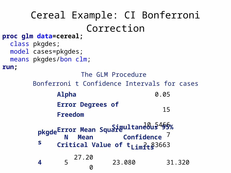
Cereal Example: CI Bonferroni Correctionproc glm data=cereal; class pkgdes; model cases=pkgdes; means pkgdes/bon clm;run;

The GLM Procedure

Bonferroni t Confidence Intervals for cases


pkgdes N MeanSimultaneous 95% Confidence

Limits4 5 27.200 23.080 31.3203 4 19.500 14.894 24.1061 5 14.600 10.480 18.7202 5 13.400 9.280 17.520

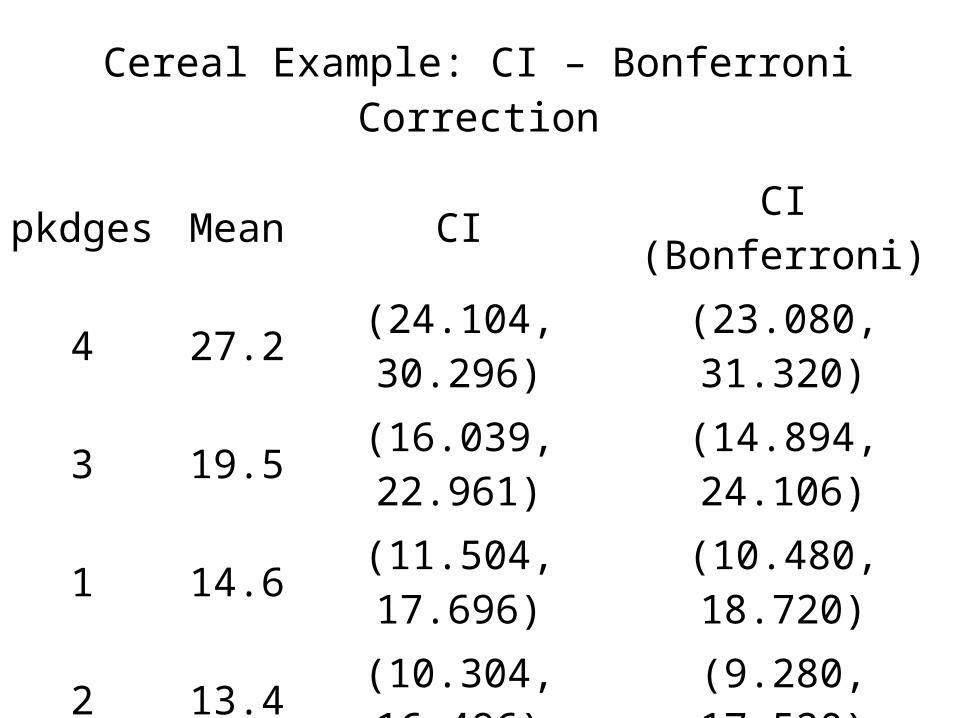
Cereal Example: CI – Bonferroni Correction

pkdges Mean CI CI (Bonferroni)4 27.2 (24.104, 30.296) (23.080, 31.320)3 19.5 (16.039, 22.961) (14.894, 24.106)1 14.6 (11.504, 17.696) (10.480, 18.720)2 13.4 (10.304, 16.496) (9.280, 17.520)

Cereal Example: Significance Testproc means data=cereal mean std stderr t probt maxdec=2; class pkgdes; var cases;run;

Analysis Variable : cases pkgdes N Obs Mean Std Dev Std Error t Value Pr > |t|

1 5 14.60 2.30 1.03 14.18 0.00012 5 13.40 3.65 1.63 8.22 0.00123 4 19.50 2.65 1.32 14.74 0.00074 5 27.20 3.96 1.77 15.35 0.0001

Cereal Example: CI for i - j

proc glm data=cereal; class pkgdes; model cases=pkgdes; means pkgdes/cldiff lsd tukey bon scheffe dunnett("2"); means pkgdes/lines tukey; run;

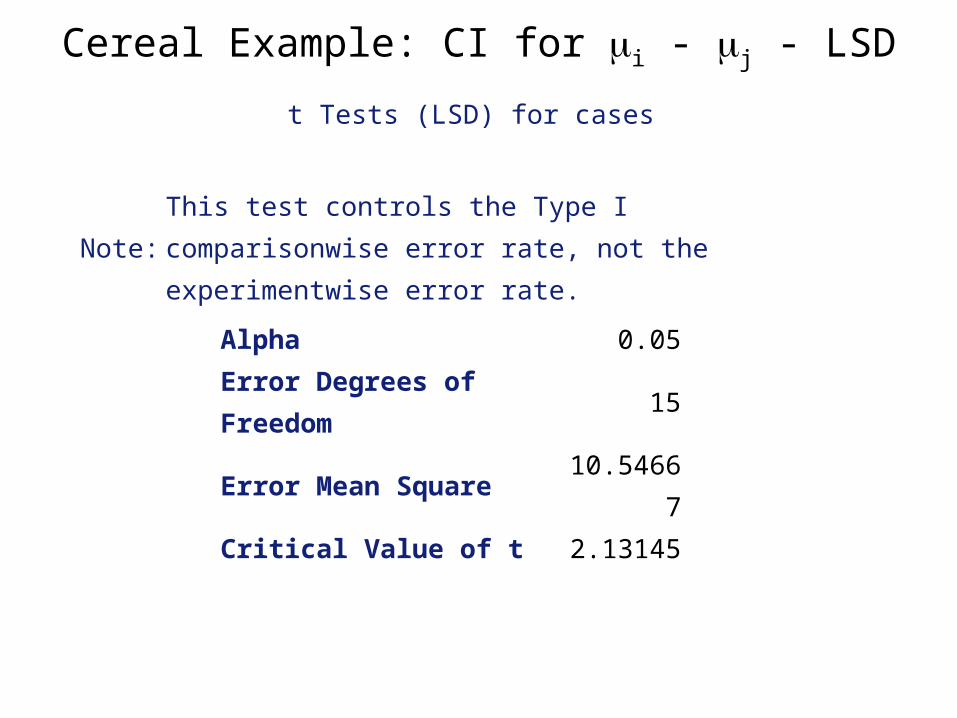
Cereal Example: CI for i - j - LSDt Tests (LSD) for cases

Note:This test controls the Type I comparisonwise error rate, not the experimentwise error rate.


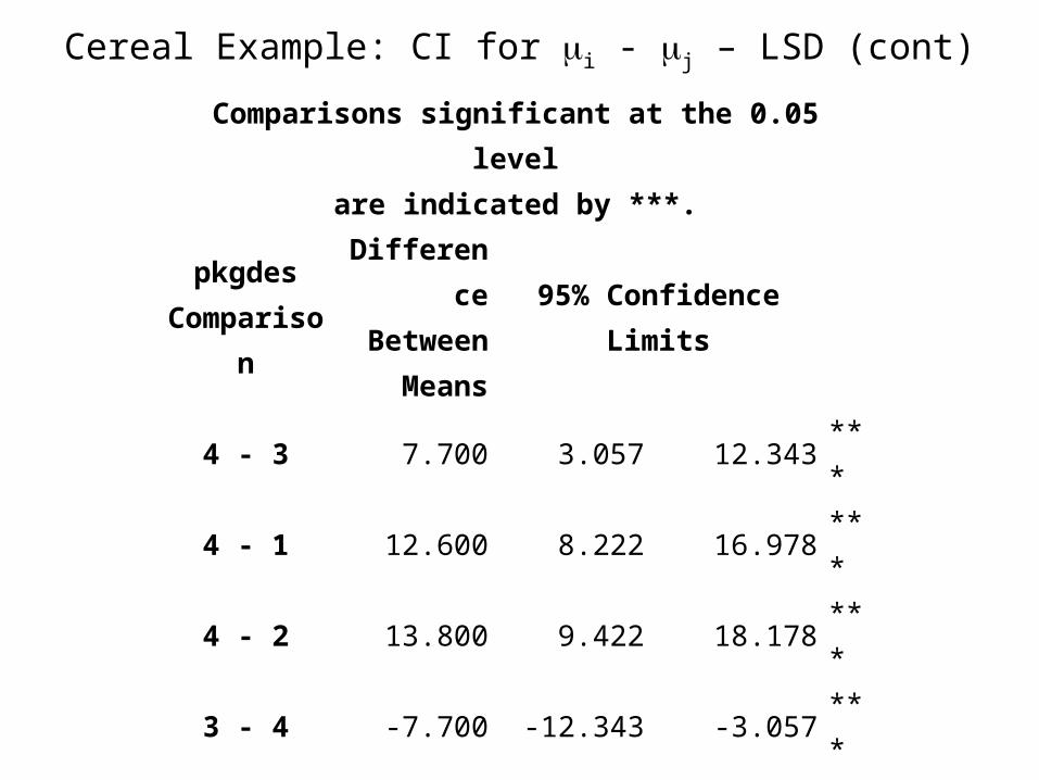
Cereal Example: CI for i - j – LSD (cont)Comparisons significant at the 0.05 level

are indicated by ***.

pkgdesComparison

DifferenceBetween

Means95% Confidence Limits

4 - 3 7.700 3.057 12.343 ***4 - 1 12.600 8.222 16.978 ***4 - 2 13.800 9.422 18.178 ***3 - 4 -7.700 -12.343 -3.057 ***3 - 1 4.900 0.257 9.543 ***3 - 2 6.100 1.457 10.743 ***1 - 4 -12.600 -16.978 -8.222 ***1 - 3 -4.900 -9.543 -0.257 ***1 - 2 1.200 -3.178 5.5782 - 4 -13.800 -18.178 -9.422 ***2 - 3 -6.100 -10.743 -1.457 ***2 - 1 -1.200 -5.578 3.178

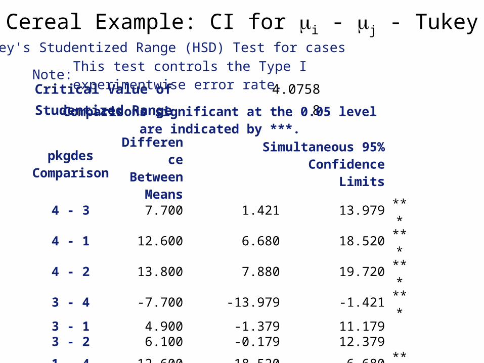
Cereal Example: CI for i - j - TukeyTukey's Studentized Range (HSD) Test for cases

Note: This test controls the Type I experimentwise error rate.

Critical Value of Studentized Range 4.07588

Comparisons significant at the 0.05 levelare indicated by ***.

pkgdesComparison

DifferenceBetween

Means

Simultaneous 95% ConfidenceLimits

4 - 3 7.700 1.421 13.979 ***4 - 1 12.600 6.680 18.520 ***4 - 2 13.800 7.880 19.720 ***3 - 4 -7.700 -13.979 -1.421 ***3 - 1 4.900 -1.379 11.1793 - 2 6.100 -0.179 12.3791 - 4 -12.600 -18.520 -6.680 ***1 - 3 -4.900 -11.179 1.3791 - 2 1.200 -4.720 7.1202 - 4 -13.800 -19.720 -7.880 ***2 - 3 -6.100 -12.379 0.1792 - 1 -1.200 -7.120 4.720

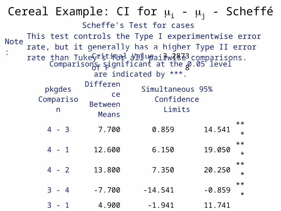
Cereal Example: CI for i - j - ScheffeScheffe's Test for cases

Note:This test controls the Type I experimentwise error rate, but it generally has a higher Type II error rate than Tukey's for all pairwise comparisons. Critical Value of F 3.28738


pkgdesComparison

DifferenceBetween

Means


4 - 3 7.700 0.859 14.541 ***4 - 1 12.600 6.150 19.050 ***4 - 2 13.800 7.350 20.250 ***3 - 4 -7.700 -14.541 -0.859 ***3 - 1 4.900 -1.941 11.741 3 - 2 6.100 -0.741 12.941 1 - 4 -12.600 -19.050 -6.150 ***1 - 3 -4.900 -11.741 1.941 1 - 2 1.200 -5.250 7.650 2 - 4 -13.800 -20.250 -7.350 ***2 - 3 -6.100 -12.941 0.741 2 - 1 -1.200 -7.650 5.250

Cereal Example: CI for i - j - BonferroniBonferroni (Dunn) t Tests for cases

Note:This test controls the Type I experimentwise error rate, but it generally has a higher Type II error rate than Tukey's for all pairwise comparisons.

Critical Value of t 3.03628Comparisons significant at the 0.05 level

are indicated by ***.

pkgdesComparison

DifferenceBetween

Means


4 - 3 7.700 1.085 14.315 ***4 - 1 12.600 6.364 18.836 ***4 - 2 13.800 7.564 20.036 ***3 - 4 -7.700 -14.315 -1.085 ***3 - 1 4.900 -1.715 11.515 3 - 2 6.100 -0.515 12.715 1 - 4 -12.600 -18.836 -6.364 ***1 - 3 -4.900 -11.515 1.715 1 - 2 1.200 -5.036 7.436 2 - 4 -13.800 -20.036 -7.564 ***2 - 3 -6.100 -12.715 0.515 2 - 1 -1.200 -7.436 5.036

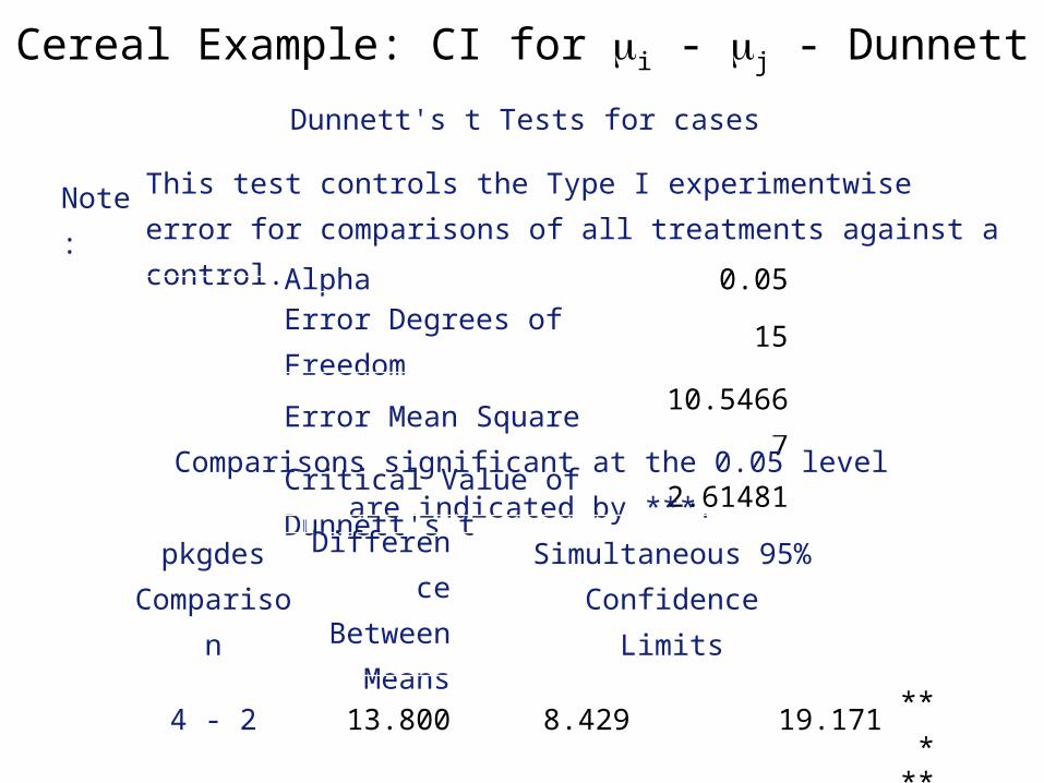
Cereal Example: CI for i - j - DunnettDunnett's t Tests for cases

Note:This test controls the Type I experimentwise error for comparisons of all treatments against a control.

Alpha 0.05Error Degrees of Freedom 15Error Mean Square 10.54667Critical Value of Dunnett's t 2.61481


pkgdesComparison

DifferenceBetween

Means


4 - 2 13.800 8.429 19.171 ***3 - 2 6.100 0.404 11.796 ***1 - 2 1.200 -4.171 6.571

Cereal Example: CI for i - j – Tukey (lines)Critical Value of Studentized Range 4.07588Minimum Significant Difference 6.1018Harmonic Mean of Cell Sizes 4.705882

Note:Cell sizes are not equal.

Means with the same letterare not significantly different.

Tukey Grouping Mean N pkgdesA 27.200 5 4 B 19.500 4 3B B 14.600 5 1B B 13.400 5 2

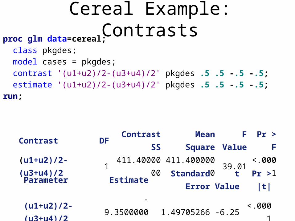
Cereal Example: Contrastsproc glm data=cereal; class pkgdes; model cases = pkgdes; contrast '(u1+u2)/2-(u3+u4)/2' pkgdes .5 .5 -.5 -.5; estimate '(u1+u2)/2-(u3+u4)/2' pkgdes .5 .5 -.5 -.5;run;

Parameter Estimate Standard Errort

ValuePr > |t|

(u1+u2)/2-(u3+u4)/2-

9.350000001.49705266 -6.25 <.0001

Contrast DF Contrast SSMean


(u1+u2)/2-(u3+u4)/2 1 411.4000000 411.4000000 39.01 <.0001

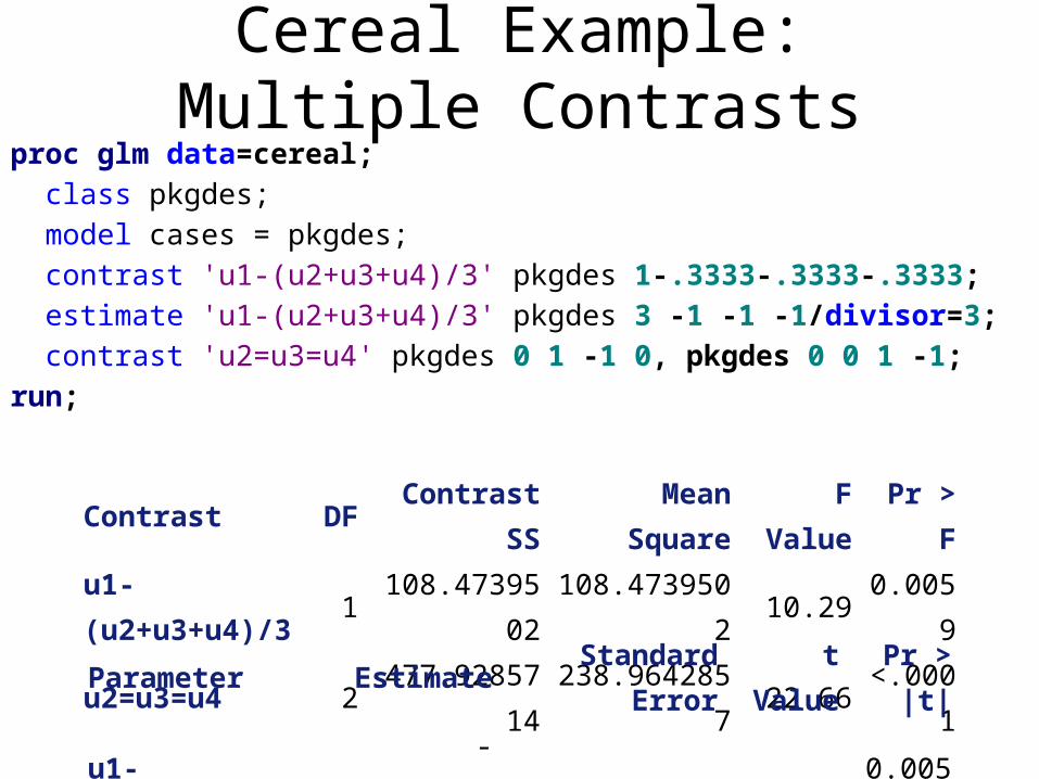
Cereal Example: Multiple Contrastsproc glm data=cereal; class pkgdes; model cases = pkgdes; contrast 'u1-(u2+u3+u4)/3' pkgdes 1-.3333-.3333-.3333; estimate 'u1-(u2+u3+u4)/3' pkgdes 3 -1 -1 -1/divisor=3; contrast 'u2=u3=u4' pkgdes 0 1 -1 0, pkgdes 0 0 1 -1;run;

Contrast DF Contrast SSMean


u1-(u2+u3+u4)/3 1 108.4739502 108.4739502 10.29 0.0059u2=u3=u4 2 477.9285714 238.9642857 22.66 <.0001

Parameter Estimate Standard Error t Value Pr > |t|u1-(u2+u3+u4)/3 -5.43333333 1.69441348 -3.21 0.0059

Training Example: (nknw742.sas)

Y = number of acceptable piecesX = hours of training (6 hrs, 8 hrs, 10 hrs, 12 hrs)n = 7

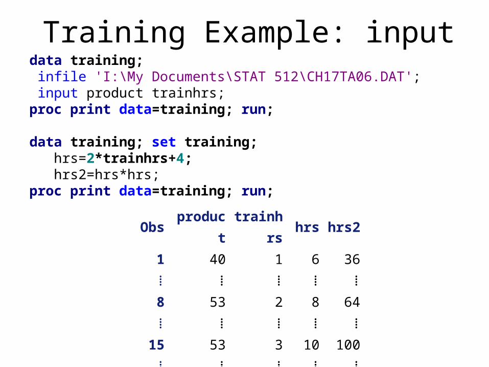
Training Example: inputdata training; infile 'I:\My Documents\STAT 512\CH17TA06.DAT'; input product trainhrs;proc print data=training; run;

data training; set training; hrs=2*trainhrs+4; hrs2=hrs*hrs;proc print data=training; run;

Obs product trainhrs hrs hrs21 40 1 6 36⁞ ⁞ ⁞ ⁞ ⁞

8 53 2 8 64⁞ ⁞ ⁞ ⁞ ⁞

15 53 3 10 100⁞ ⁞ ⁞ ⁞ ⁞

22 63 4 12 144⁞ ⁞ ⁞ ⁞ ⁞

Training Example: ANOVAproc glm data=training; class trainhrs; model product=hrs trainhrs / solution;run;

Parameter Estimate Standard Errort

ValuePr > |t|

Intercept 32.28571429 B 6.09421494 5.30 <.0001hrs 2.42857143 B 0.55174430 4.40 0.0002trainhrs 1 -6.85714286 B 2.91955639 -2.35 0.0274trainhrs 2 -1.85714286 B 1.91129831 -0.97 0.3409trainhrs 3 0.00000000 B . . .trainhrs 4 0.00000000 B . . .

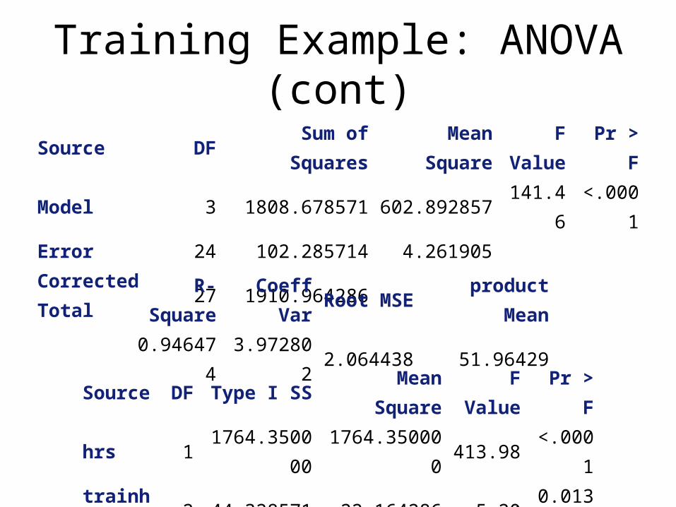
Training Example: ANOVA (cont)




R-Square Coeff Var Root MSE product Mean0.946474 3.972802 2.064438 51.96429

Source DF Type I SS Mean Square F Value Pr > Fhrs 1 1764.350000 1764.350000 413.98 <.0001trainhrs 2 44.328571 22.164286 5.20 0.0133

Training Example: ScatterplotTitle1 h=3 'product vs. hrs';axis1 label=(h=2);axis2 label=(h=2 angle=90);symbol1 v = circle i = rl;proc gplot data=training;

plot product*hrs/haxis=axis1 vaxis=axis2;run;

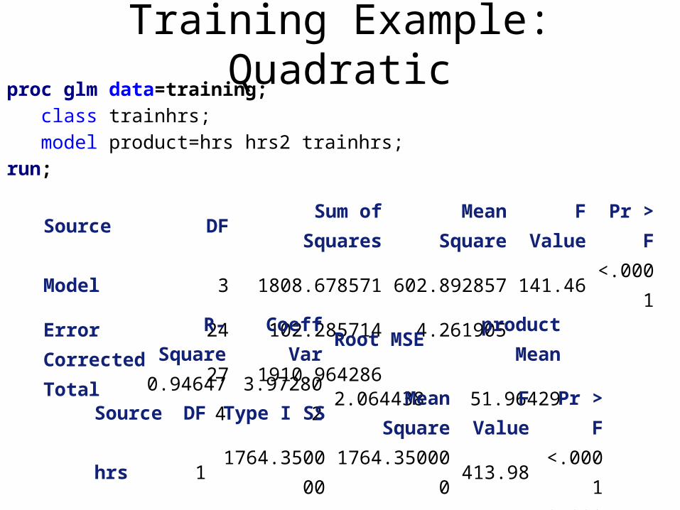
Training Example: Quadraticproc glm data=training; class trainhrs; model product=hrs hrs2 trainhrs;run;




R-Square Coeff Var Root MSE product Mean0.946474 3.972802 2.064438 51.96429

Source DF Type I SSMean


hrs 1 1764.350000 1764.350000 413.98 <.0001hrs2 1 43.750000 43.750000 10.27 0.0038trainhrs 1 0.578571 0.578571 0.14 0.7158

Rust Example: (nknw712.sas)

Y = effectiveness of the rust inhibitorscoded score, the higher means less rust

X has 4 levels, the brands are A, B, C, Dn = 10

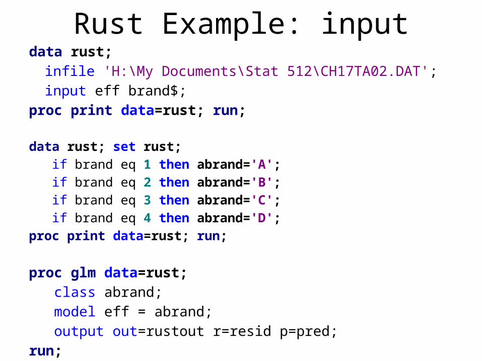
Rust Example: inputdata rust;

infile 'H:\My Documents\Stat 512\CH17TA02.DAT';input eff brand$;

proc print data=rust; run;

data rust; set rust; if brand eq 1 then abrand='A'; if brand eq 2 then abrand='B'; if brand eq 3 then abrand='C'; if brand eq 4 then abrand='D';proc print data=rust; run;

proc glm data=rust; class abrand; model eff = abrand; output out=rustout r=resid p=pred;run;

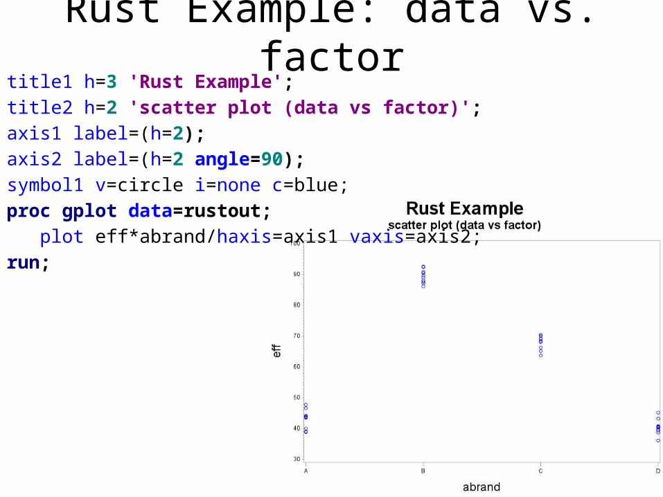
Rust Example: data vs. factortitle1 h=3 'Rust Example';title2 h=2 'scatter plot (data vs factor)';axis1 label=(h=2);axis2 label=(h=2 angle=90);symbol1 v=circle i=none c=blue;proc gplot data=rustout;

plot eff*abrand/haxis=axis1 vaxis=axis2; run;

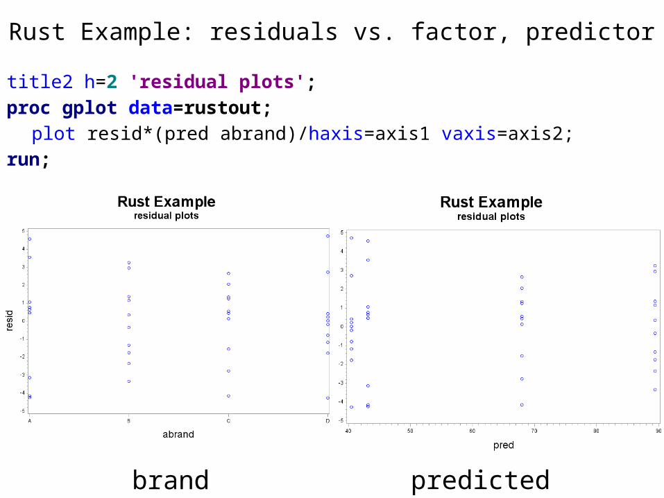
Rust Example: residuals vs. factor, predictortitle2 h=2 'residual plots';proc gplot data=rustout;

plot resid*(pred abrand)/haxis=axis1 vaxis=axis2;run;

brand predicted value

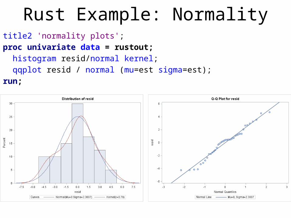
Rust Example: Normalitytitle2 'normality plots';proc univariate data = rustout; histogram resid/normal kernel; qqplot resid / normal (mu=est sigma=est); run;

Solder Example (nknw768.sas)

Y = strength of jointX = type of solder flux (there are 5 types in the

study)n = 8

Solder Example: input/diagnosticsdata solder; infile 'I:\My Documents\Stat 512\CH18TA02.DAT'; input strength type;proc print data=solder; run;

title1 h=3 'Solder Example';title2 h=2 'scatterplot';axis1 label=(h=2);axis2 label=(h=2 angle=90);symbol1 v=circle i=none c=red;proc gplot data=solder; plot strength*type/haxis=axis1 vaxis=axis2;run;

Solder Example: scatterplot

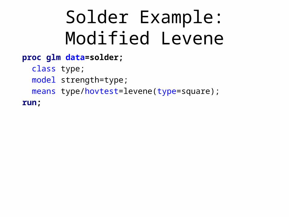
Solder Example: Modified Leveneproc glm data=solder; class type; model strength=type; means type/hovtest=levene(type=square);run;

Solder Example: Modified Levene (cont)Source DF Sum of Squares Mean Square F Value Pr > FModel 4 353.6120850 88.4030212 41.93 <.0001Error 35 73.7988250 2.1085379Corrected Total 39 427.4109100

R-Square Coeff Var Root MSE strength Mean0.827335 10.22124 1.452081 14.20650

Source DF Type I SS Mean Square F Value Pr > Ftype 4 353.6120850 88.4030212 41.93 <.0001

Levene's Test for Homogeneity of strength VarianceANOVA of Squared Deviations from Group Means



type 4 132.3 33.0858 3.57 0.0153Error 35 324.6 9.2751

Solder Example: Modified Levene (cont)

Level oftype

Nstrength

Mean Std Dev

1 8 15.4200000 1.23713956

2 8 18.5275000 1.25297076

3 8 15.0037500 2.48664397

4 8 9.7412500 0.81660337

5 8 12.3400000 0.76941536

Solder Example: Weighted Least Squares

proc means data=solder; var strength; by type; output out=weights var=s2;run;

data weights; set weights; wt=1/s2;

Solder Example: Weighted Least Squares (cont)

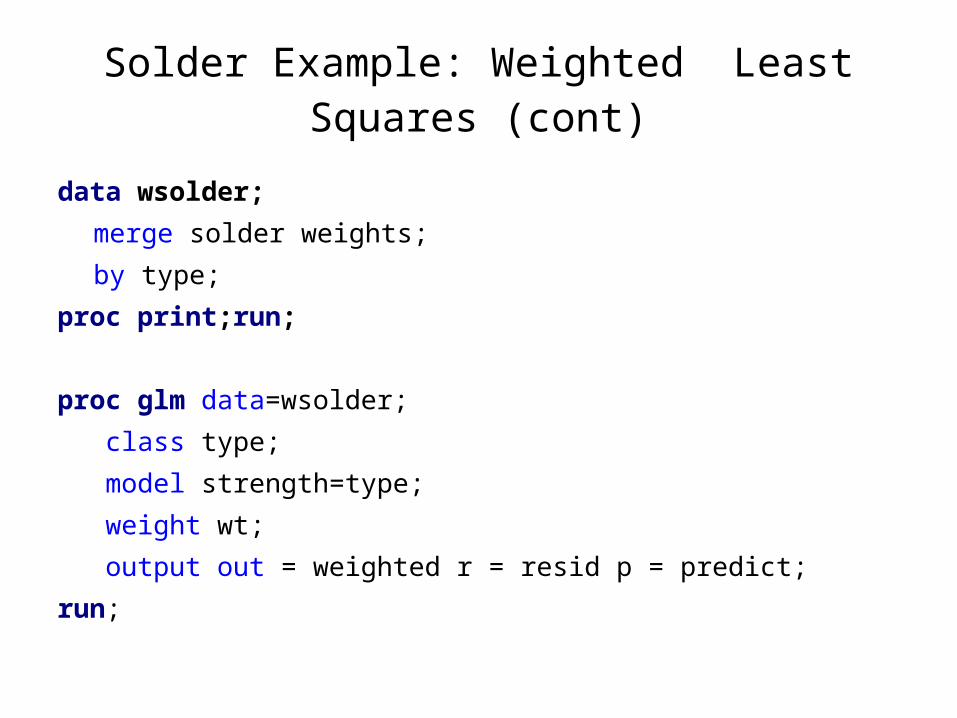
data wsolder; merge solder weights; by type;

proc print;run;

proc glm data=wsolder; class type; model strength=type; weight wt; output out = weighted r = resid p = predict; run;


Dependent Variable: strength

Weight: wt

From before: F = 41.93, R2 = 0.827335




R-Square Coeff Var Root MSE strength Mean0.902565 7.766410 1.00000 12.87596


data residplot; set weighted; resid1 = sqrt(wt)*resid;

title2 h=2 'Weighted data - residual plot';symbol1 v=circle i=none;proc gplot data=residplot; plot resid1*(predict type)/vref=0 haxis=axis1 vaxis=axis2;run;

anova: graphical. cereal example: nknw677.sas y = number of cases of cereal sold (cases) x = design...

Documents

cereal example

cereal plot cases

cereal var cases

cereal title2 h

cereal package pkgdes

input data cereal infile

cont slide

graphical slide