ANOVA (Analysis of Variance)

andExperimentation

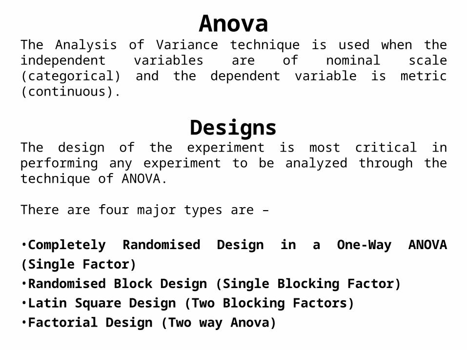
AnovaThe Analysis of Variance technique is used when the independent variables are of nominal scale (categorical) and the dependent variable is metric (continuous).

DesignsThe design of the experiment is most critical in performing any experiment to be analyzed through the technique of ANOVA.

There are four major types are –

•Completely Randomised Design in a One-Way ANOVA (Single Factor)

•Randomised Block Design (Single Blocking Factor)

•Latin Square Design (Two Blocking Factors)

•Factorial Design (Two way Anova)

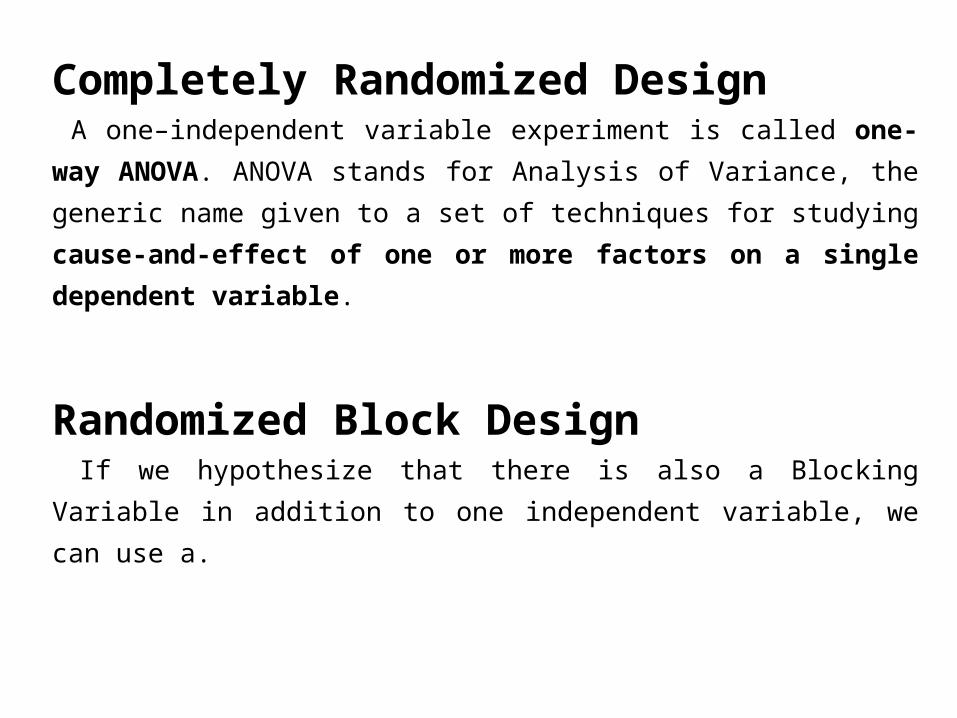
Completely Randomized Design A one–independent variable experiment is called one-way ANOVA. ANOVA

stands for Analysis of Variance, the generic name given to a set of techniques

for studying cause-and-effect of one or more factors on a single dependent

variable.

Randomized Block Design If we hypothesize that there is also a Blocking Variable in addition to one

independent variable, we can use a.

One-Way ANOVA

Researchers are often interested in examining the differences in the

mean values of the dependent variable for several categories of a

single independent variable or factor.

One dependent (metric) variable.

There is only one categorical independent variable. Variable is called a

Factor. Each category of an independent variable is called a level.

The independent variable may be different levels of prices, or different pack sizes,

or different product colours, and the effect (dependent variable) could be sales,

preferences or attitudes towards the brand.

Some more examples:

• Do the various segments differ in terms of their volume of product consumption?

• Do the brand evaluations of groups exposed to different commercials vary?

Relationship with t-test

Analysis of variance (ANOVA) is used as a test of means for two or more populations, hence extension of t-test for difference of means. The null hypothesis, typically, is that all means are equal.

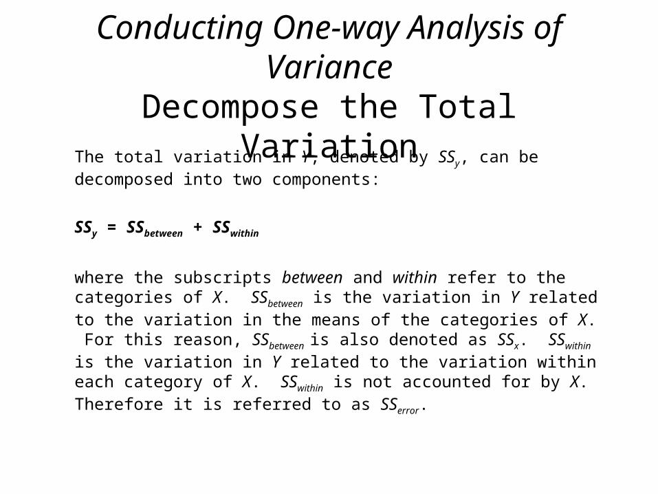
Conducting One-way Analysis of Variance

Decompose the Total VariationThe total variation in Y, denoted by SSy, can be decomposed into two components:

 

SSy = SSbetween + SSwithin

 

where the subscripts between and within refer to the categories of X. SSbetween is the variation in Y related to the variation in the means of the categories of X. For this reason, SSbetween is also denoted as SSx. SSwithin is the variation in Y related to the variation within each category of X. SSwithin is not accounted for by X. Therefore it is referred to as SSerror.

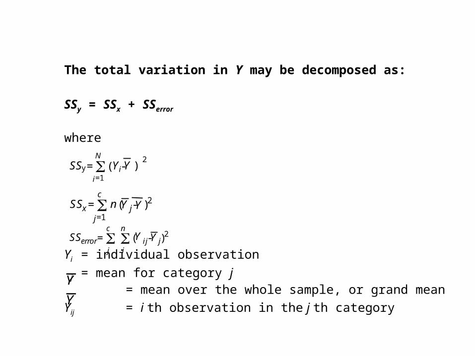
The total variation in Y may be decomposed as:

SSy = SSx + SSerror

where

  

 

Yi = individual observation

j = mean for category j = mean over the whole sample, or grand mean

Yij = i th observation in the j th category

SSy= (Yi-Y )2

i=1

N

SSx = n (Y j -Y )2j=1

c

SSerror= i

n(Y ij-Y j)

2j

c

Y

Y

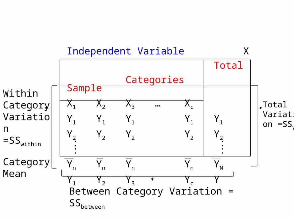
Independent Variable X

Total

Categories Sample

X1 X2 X3 … Xc

Y1 Y1 Y1 Y1 Y1

Y2 Y2 Y2 Y2 Y2 : : : :Yn Yn Yn Yn YN

Y1 Y2 Y3 Yc Y

Within Category Variation =SSwithin

Between Category Variation = SSbetween

Total Variation =SSy

Category Mean

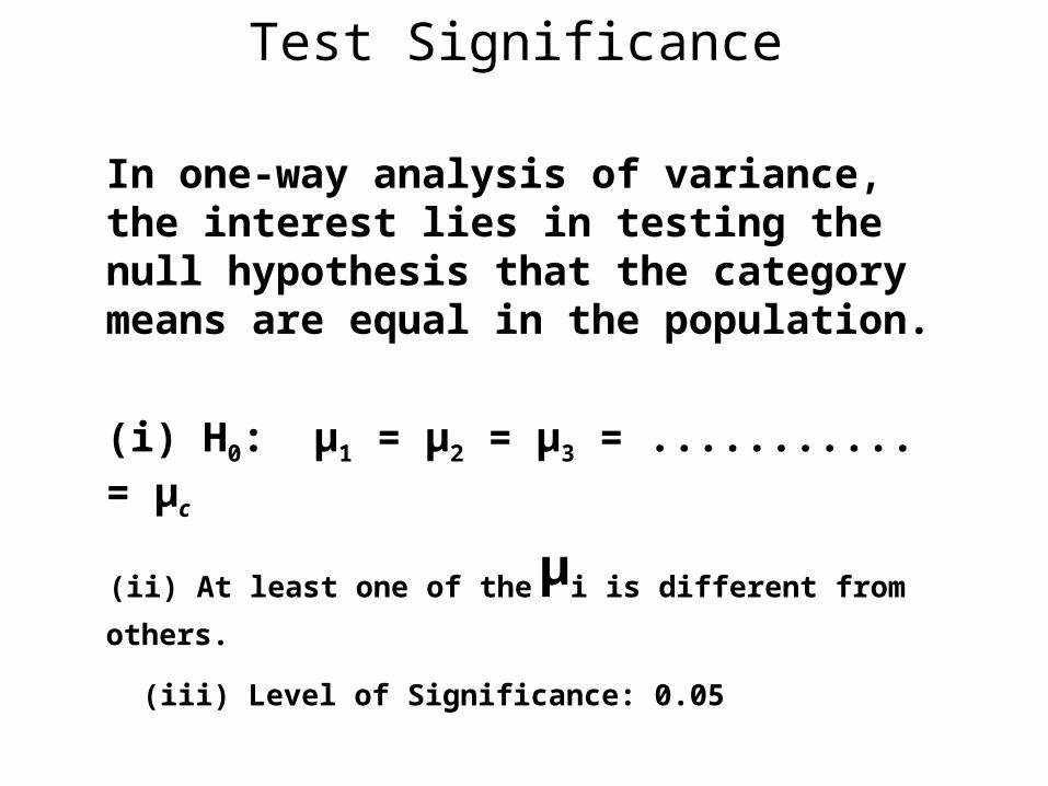
Test Significance

In one-way analysis of variance, the interest lies in testing the null hypothesis that the category means are equal in the population.

 

(i) H0: µ1 = µ2 = µ3 = ........... = µc

(ii) At least one of the µi is different from others.

(iii) Level of Significance: 0.05

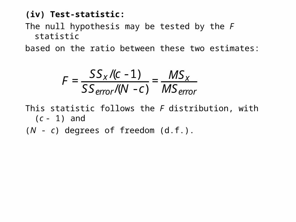
(iv) Test-statistic:

The null hypothesis may be tested by the F statistic

based on the ratio between these two estimates:

 

 

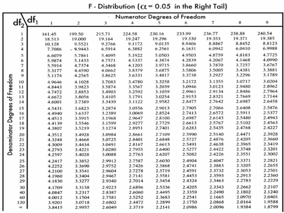
This statistic follows the F distribution, with (c - 1) and

(N - c) degrees of freedom (d.f.).

F = SSx /(c - 1)

SSerror/(N - c) = MSx

MSerror

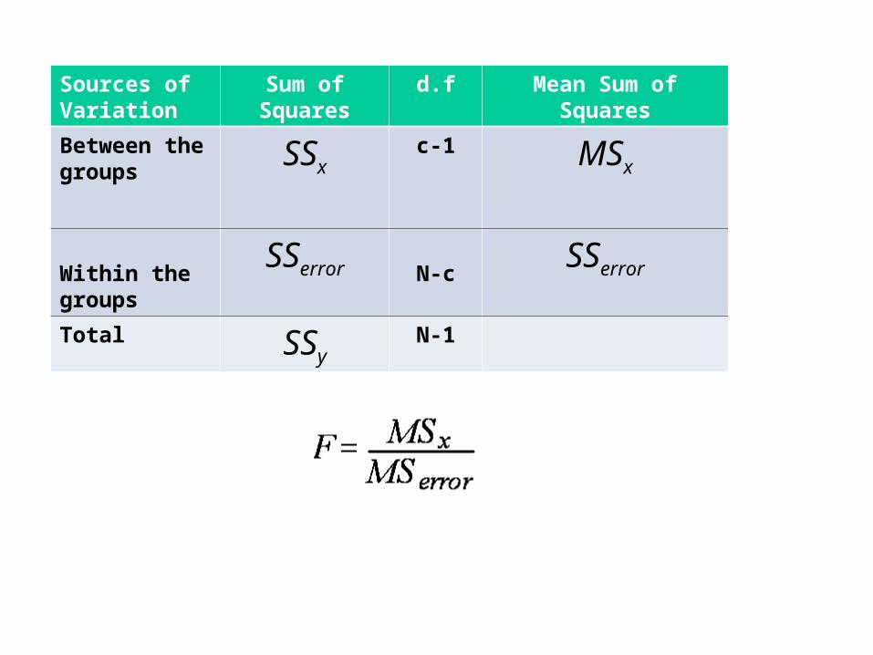
Sources of Variation

Sum of Squares d.f Mean Sum of Squares

Between the groups

SSxc-1 MSx

Within the groups

SSerror N-cSSerror

Total SSyN-1

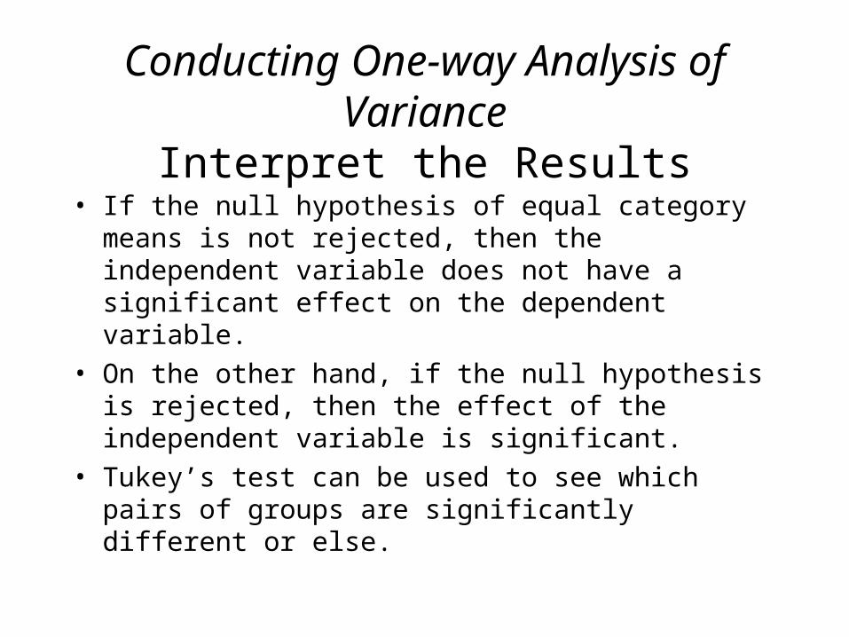
Conducting One-way Analysis of Variance

Interpret the Results• If the null hypothesis of equal category means is not

rejected, then the independent variable does not have a significant effect on the dependent variable.

• On the other hand, if the null hypothesis is rejected, then the effect of the independent variable is significant.

• Tukey’s test can be used to see which pairs of groups are significantly different or else.

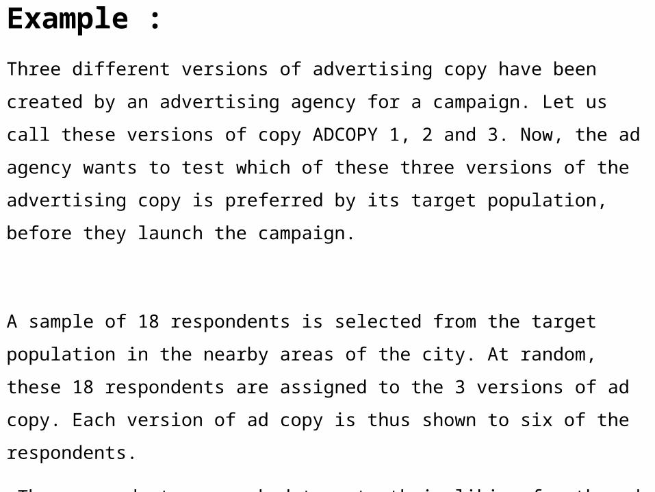
Example :

Three different versions of advertising copy have been created by an advertising

agency for a campaign. Let us call these versions of copy ADCOPY 1, 2 and 3. Now,

the ad agency wants to test which of these three versions of the advertising copy is

preferred by its target population, before they launch the campaign.

A sample of 18 respondents is selected from the target population in the nearby areas of

the city. At random, these 18 respondents are assigned to the 3 versions of ad copy.

Each version of ad copy is thus shown to six of the respondents.

The respondents are asked to rate their liking for the ad copy shown to them on a scale

of 1 to 10. (1 = Not liked at all, 10 = Liked a lot, and other values in between these

two). The ratings given by the 18 respondents are tabulated.

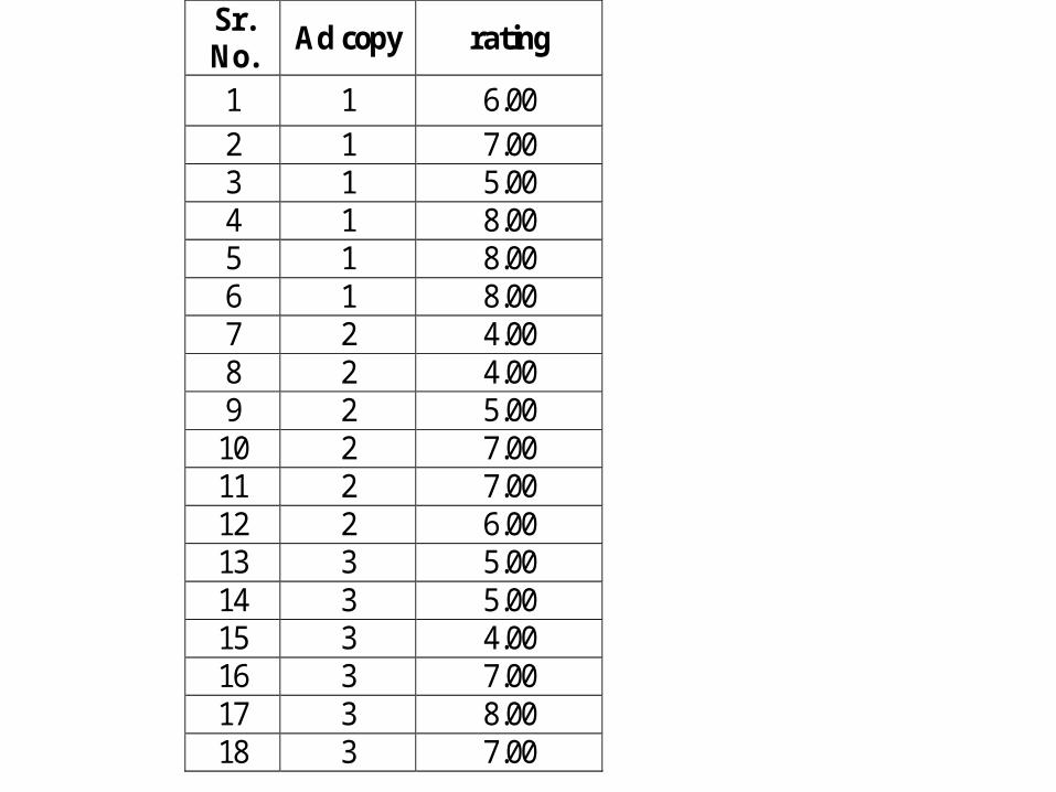
Sr. No.

Ad copy rating

1 1 6.00

2 1 7.00 3 1 5.00 4 1 8.00 5 1 8.00 6 1 8.00 7 2 4.00 8 2 4.00 9 2 5.00 10 2 7.00 11 2 7.00 12 2 6.00 13 3 5.00 14 3 5.00 15 3 4.00 16 3 7.00 17 3 8.00 18 3 7.00

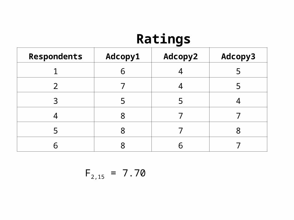
RatingsRespondents Adcopy1 Adcopy2 Adcopy3

1 6 4 5

2 7 4 5

3 5 5 4

4 8 7 7

5 8 7 8

6 8 6 7

F2,15 = 7.70

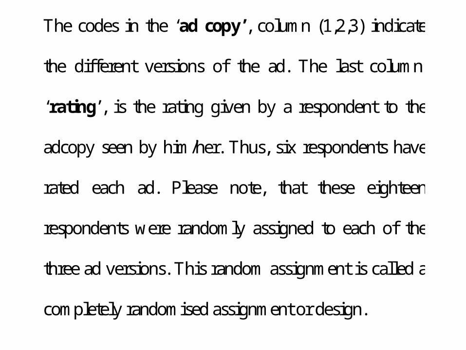
The codes in the ‘ad copy’, column (1,2,3) indicate

the different versions of the ad. The last column,

‘rating’, is the rating given by a respondent to the

adcopy seen by him/her. Thus, six respondents have

rated each ad. Please note, that these eighteen

respondents were randomly assigned to each of the

three ad versions. This random assignment is called a

completely randomised assignment or design.

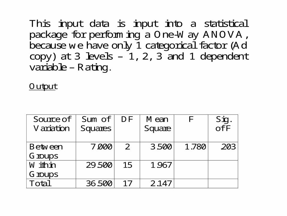
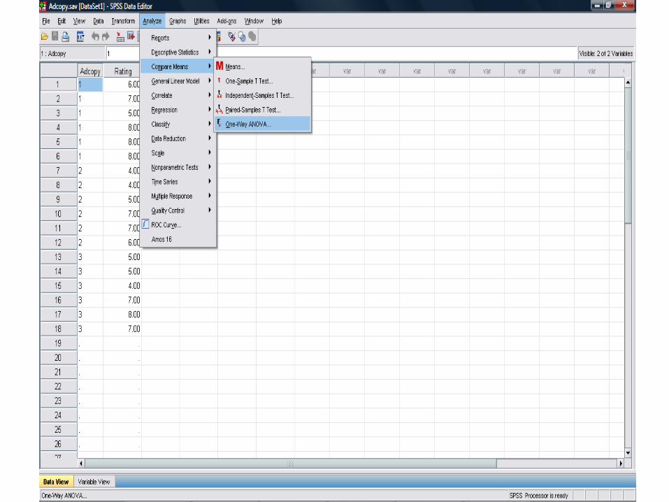
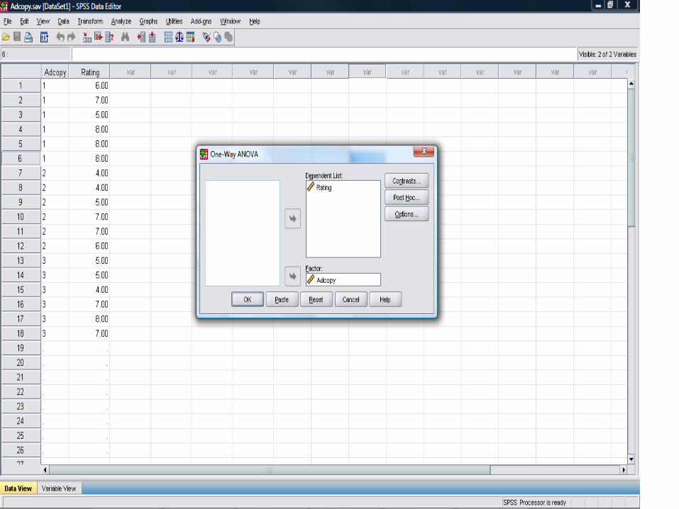
This input data is input into a statistical package for performing a One-Way ANOVA, because we have only 1 categorical factor (Ad copy) at 3 levels – 1, 2, 3 and 1 dependent variable – Rating. Output

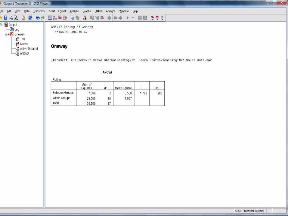
Source of Variation

Sum of Squares

DF Mean Square

F Sig. of F

Between Groups

7.000 2 3.500 1.780 .203

Within Groups

29.500 15 1.967

Total 36.500 17 2.147

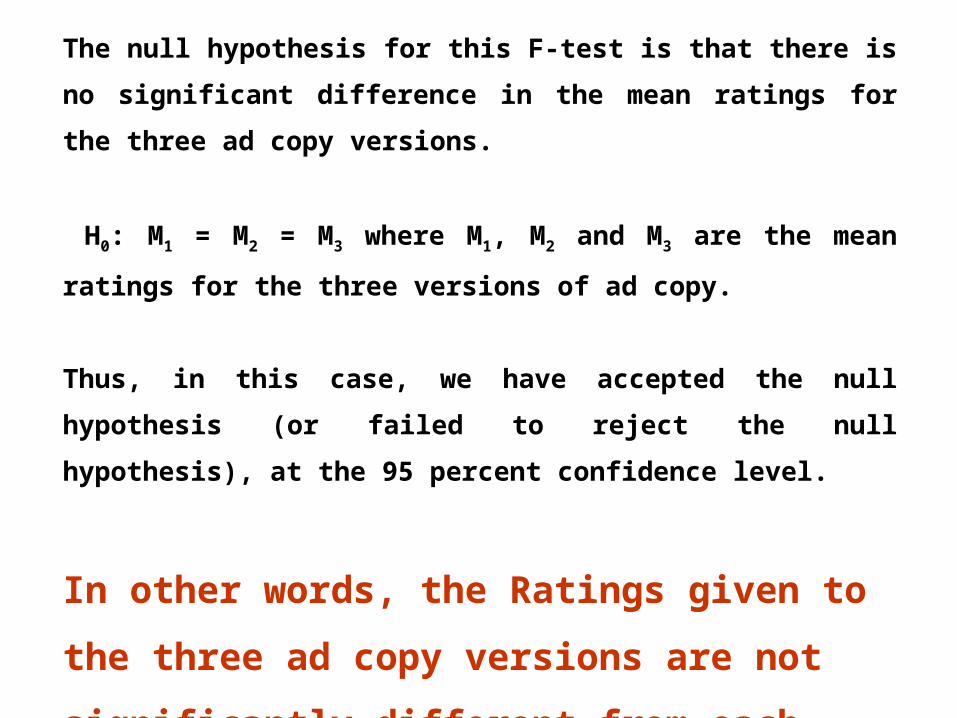
The null hypothesis for this F-test is that there is no significant difference

in the mean ratings for the three ad copy versions.

H0: M1 = M2 = M3 where M1, M2 and M3 are the mean ratings for the

three versions of ad copy.

Thus, in this case, we have accepted the null hypothesis (or failed to

reject the null hypothesis), at the 95 percent confidence level.

In other words, the Ratings given to the three ad

copy versions are not significantly different from

each other.

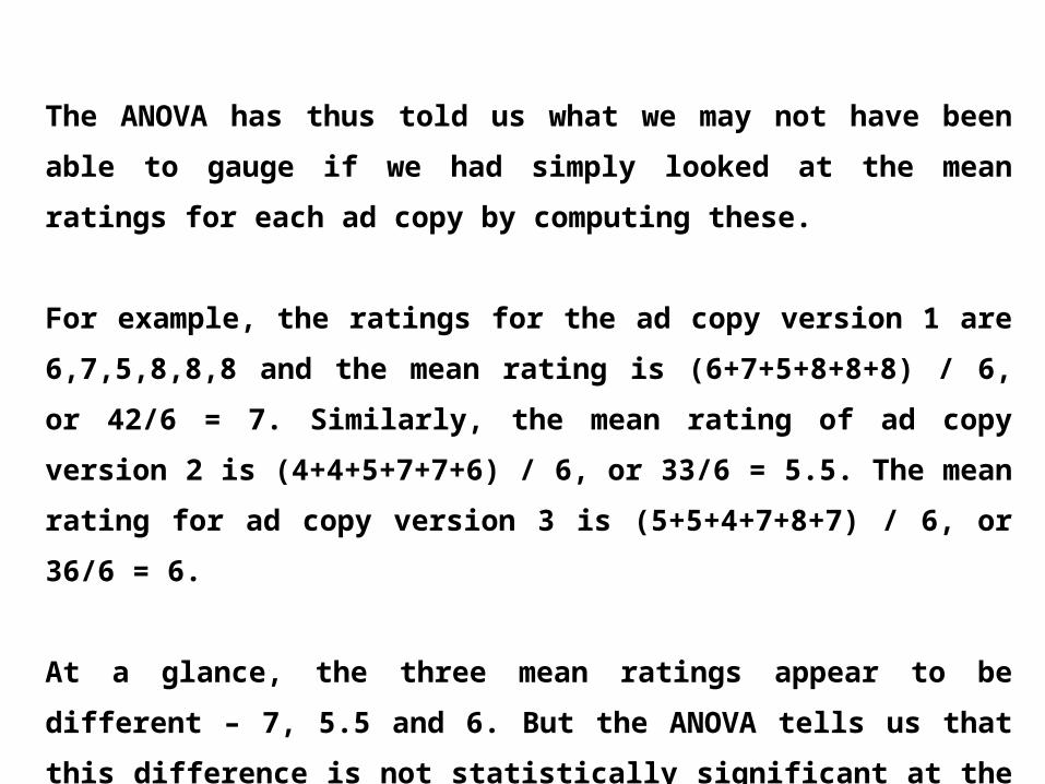
The ANOVA has thus told us what we may not have been able to gauge if we

had simply looked at the mean ratings for each ad copy by computing these.

For example, the ratings for the ad copy version 1 are 6,7,5,8,8,8 and the

mean rating is (6+7+5+8+8+8) / 6, or 42/6 = 7. Similarly, the mean rating of

ad copy version 2 is (4+4+5+7+7+6) / 6, or 33/6 = 5.5. The mean rating for ad

copy version 3 is (5+5+4+7+8+7) / 6, or 36/6 = 6.

At a glance, the three mean ratings appear to be different – 7, 5.5 and 6. But

the ANOVA tells us that this difference is not statistically significant at the 95

percent confidence level.

It does this by performing an F-test.

1.

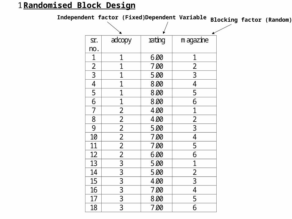
Randomised Block Design

sr. no.

adcopy rating magazine

1 1 6.00 1 2 1 7.00 2 3 1 5.00 3 4 1 8.00 4 5 1 8.00 5 6 1 8.00 6 7 2 4.00 1 8 2 4.00 2 9 2 5.00 3

10 2 7.00 4 11 2 7.00 5 12 2 6.00 6 13 3 5.00 1 14 3 5.00 2 15 3 4.00 3 16 3 7.00 4 17 3 8.00 5 18 3 7.00 6

Dependent Variable Blocking factor (Random)Independent factor (Fixed)

We have made a slightly different assumption in this case.

We assume that the three versions of the adcopy were each

used in 6 different magazines. These six magazines are

coded 1, 2, 3, 4, 5, 6 and appear in the column titled

“magazine”. Out of the people who saw these ads, 18

randomly chosen respondents are picked, one from each

magazine who saw a particular version of ad. Thus, we

finally have one respondent who has seen a given version

of the ad in a given magazine. In other words, we have one

respondent for every combination of magazine and adcopy.

Hypothesis

1. The assignment of our sample of 18 in the above manner assumes that

the magazine in which the version of adcopy appears may have an

impact on the ratings. We can test this hypothesis - in fact, two

hypotheses - by doing an ANOVA with a randomized block design.

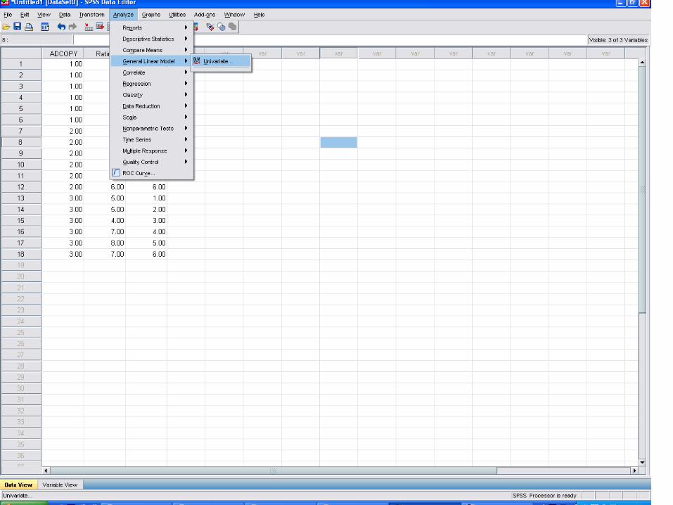
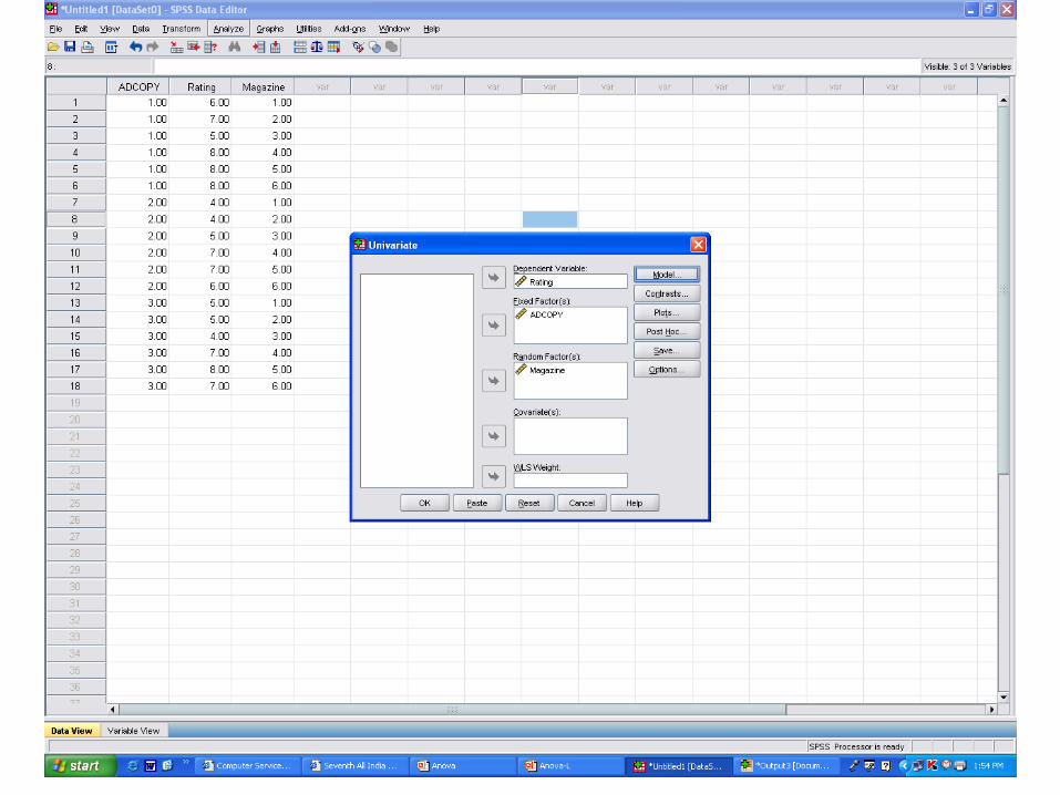
2. For this purpose, we use the variable ‘Rating’ as the dependent

variable, and ‘Adcopy’ as the factor, and ‘Magazine’ as the block.

3. A block is defined as some variable which could affect the relationship

between the independent factor and the dependent variable under study in an

ANOVA. In our example, the magazine in which the advertisement appears

could influence the Rating given to Adcopy by the respondents. We are trying

to remove the effect of the magazine used, by "blocking" its effect, or treating

the block separately.

4. If we do not block on a variable, its effect gets included with the error

(residual) term. This may lead to wrong conclusions about the relationship

between the independent and dependent variables. In that sense, a randomised

block design is more "powerful" than a simple one-way ANOVA, if the block

effect is significantly influencing the relationship.

First null hypothesis

Mean rating of the ADCOPY is the same for all 3 versions.

Second null hypothesis

‘Block’ used (Magazine in this case) has no effect on mean ratings

given to ADCOPY versions by respondents.

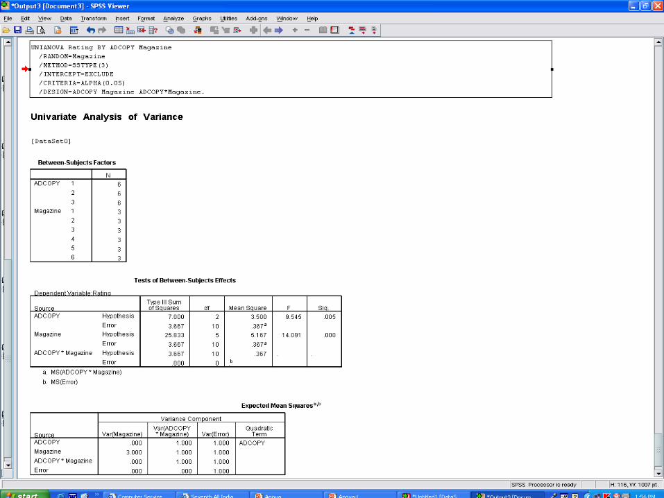
Blocking Factor being considered separately has now

led us to a different conclusion from that in a

completely randomized test of the same basic data.

This makes the randomized block test a better test

when we suspect that a blocking factor affects the

relationship between the independent variable and

the dependent variable.

Latin Square Design

The Latin Square Design is an extension of the Randomised Block

Design. It consists of one independent variable (FACTOR) and two

Blocks, instead of one which we saw in the Randomised Block Design.

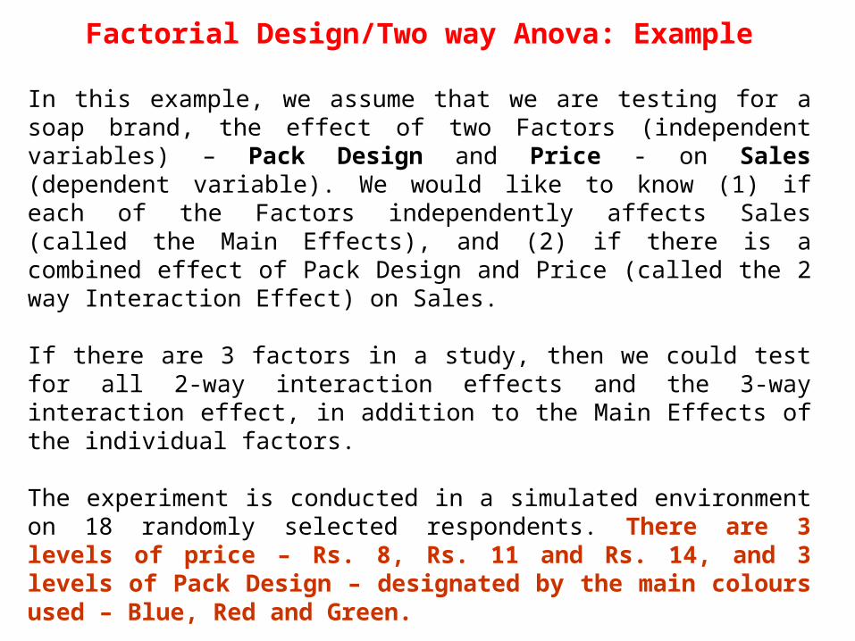
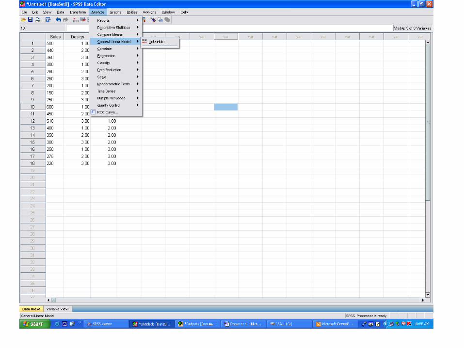
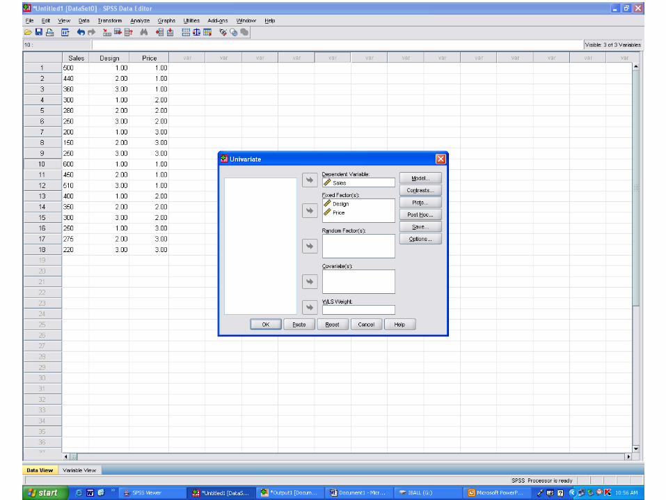
Factorial Design/Two way Anova: Example

In this example, we assume that we are testing for a soap brand, the effect of two Factors (independent variables) – Pack Design and Price - on Sales (dependent variable). We would like to know (1) if each of the Factors independently affects Sales (called the Main Effects), and (2) if there is a combined effect of Pack Design and Price (called the 2 way Interaction Effect) on Sales.

If there are 3 factors in a study, then we could test for all 2-way interaction effects and the 3-way interaction effect, in addition to the Main Effects of the individual factors.

The experiment is conducted in a simulated environment on 18 randomly selected respondents. There are 3 levels of price – Rs. 8, Rs. 11 and Rs. 14, and 3 levels of Pack Design – designated by the main colours used – Blue, Red and Green.

The coding of these variables is 1, 2, 3 respectively for Rs. 8, 11 and 14 and 1, 2, 3 for Blue, Red and Green in the case of Pack Design.

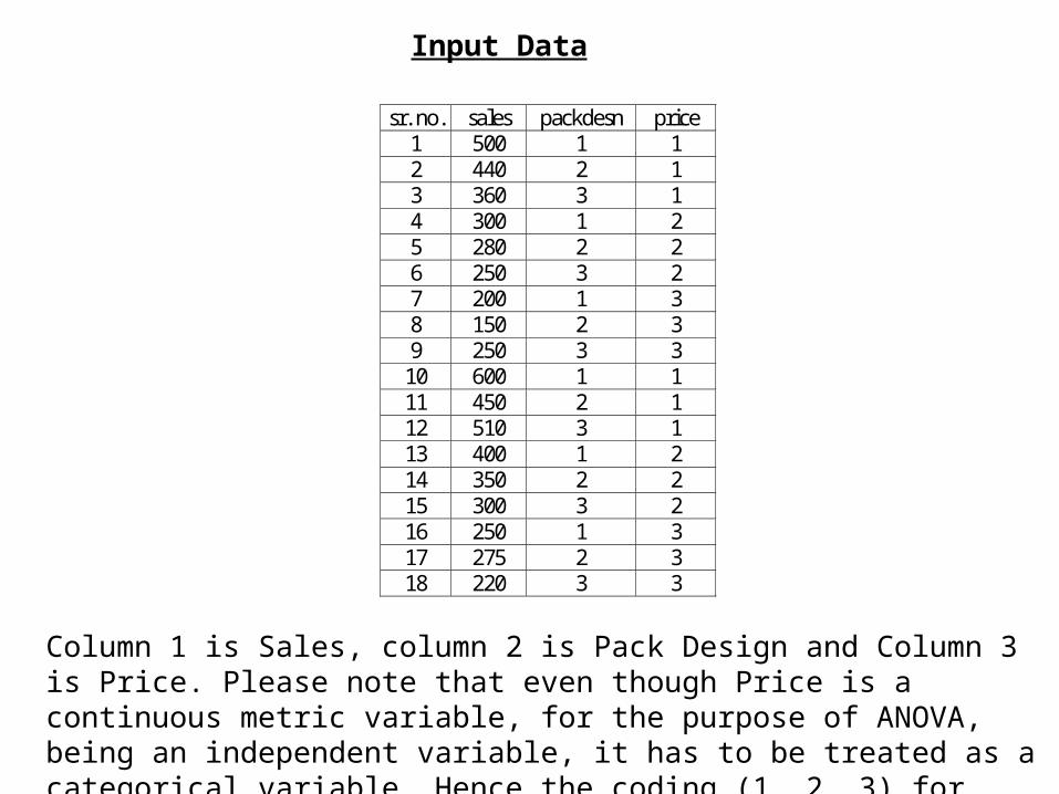
Input Data

sr. no. sales packdesn price

1 500 1 1 2 440 2 1 3 360 3 1 4 300 1 2 5 280 2 2 6 250 3 2 7 200 1 3 8 150 2 3 9 250 3 3

10 600 1 1 11 450 2 1 12 510 3 1 13 400 1 2 14 350 2 2 15 300 3 2 16 250 1 3 17 275 2 3 18 220 3 3

Column 1 is Sales, column 2 is Pack Design and Column 3 is Price. Please note that even though Price is a continuous metric variable, for the purpose of ANOVA, being an independent variable, it has to be treated as a categorical variable. Hence the coding (1, 2, 3) for Price.

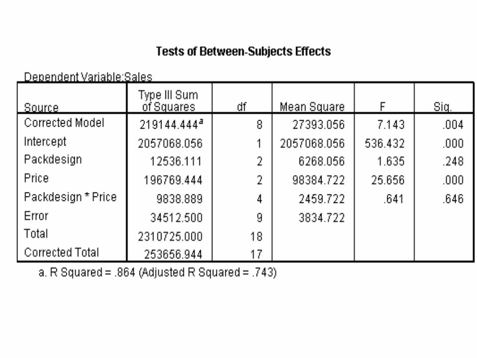
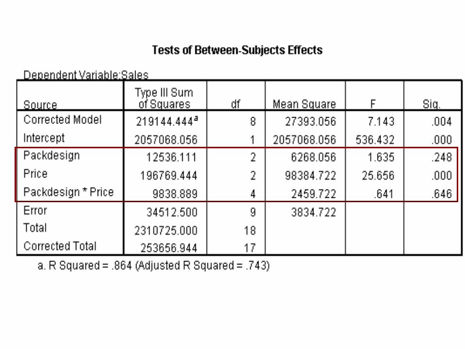
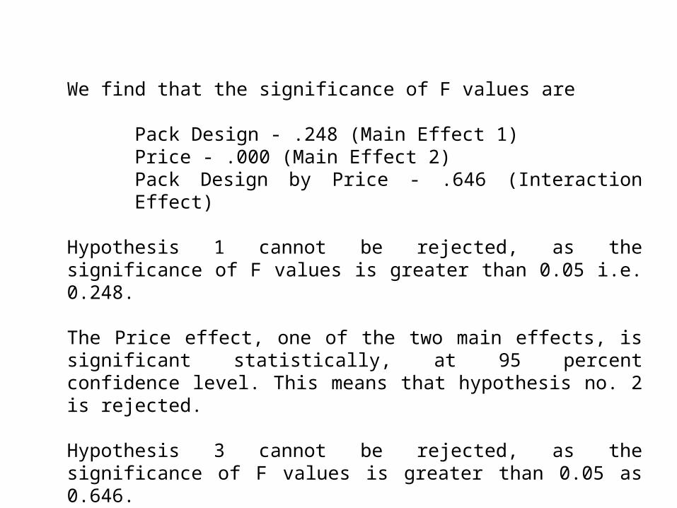
We find that the significance of F values are

Pack Design - .248 (Main Effect 1)Price - .000 (Main Effect 2)Pack Design by Price - .646 (Interaction Effect)

Hypothesis 1 cannot be rejected, as the significance of F values is greater than 0.05 i.e. 0.248.

The Price effect, one of the two main effects, is significant statistically, at 95 percent confidence level. This means that hypothesis no. 2 is rejected.

Hypothesis 3 cannot be rejected, as the significance of F values is greater than 0.05 as 0.646.

Thus, we conclude that Price alone has an impact on Sales. Neither Pack Design alone nor the combination of Pack Design with Price have any significant impact on Sales of the toilet soap.