antenna placement on large platforms

Sonnet Software, Inc. (315)453-3096 [email protected]

1

Antenna Placement on Large Platforms: Microwave Studio A-Solver

Using the Asymptotic Solver in CST Studio Suite 2011Microwave Studio® at Sonnet Software, Inc.Dr. James R Willhite Shrikrishna Hegde

UHF antenna on 99x131’aircraft

SHF antenna on 137x32m ship on sea water

Aircraft Example


2

Modeling antennas mounted on large platforms presents difficulties. The structure of the antenna and the wavelength may be quite small compared to the platform. These simulations typically cannot be done on workstations with FEM or FDTD techniques. The goals in this study are to use the asymptotic solver in Microwave Studio to see the effects of the platform on the antenna patterns and to estimate coupling between the antennas. An aircraft 98.6’ long with a wing span of 131.4’ was chosen as the first example. At 400MHz the aircraft is 40 by 53.4 λ.

A1

A2

A3

A4

Blade Antenna


3

A simple UHF blade (300 – 600 MHz) had been designed using an infinite ground. It was re-simulated in the transient solver using a short cylindrical ground. The radius of the ground was that of the aircraft and this simulation was used to obtain a far field pattern with a neighboring environment similar to placement on the aircraft. This simulation required 37 minutes and 1.7 Gbytes.

Blade Antenna Pattern on Cylindrical Ground.


4

This far field pattern at 400 MHz from the T-solver was used at the antenna locations as the source for the A-solver. The actual antennas will not be placed in the A-solver model; only their far field patterns from one of the other solvers in MWS.

Antenna 1 Source & Far Field Pattern


5

The far field pattern from the blade antenna was defined as a far field source in the aircraft model. The A-solver meshes the surfaces and calculates the radiation using a shooting bouncing ray technique.

source

The far field pattern for Antenna 1 from the A-solver is similar to that from the source but the directivity has increased 2.5 dB. The aircraft was modeled as lossless metal but loss could be added.

resultant far field pattern


6

Antenna 2 Source & Far Field PatternThe location of antenna 2 is very similar to that of the blade on the cylindrical ground. Therefore it is not too surprising that the shape of the far field and the peak directivity have not changed significantly.

source



7

Antenna 3 Source & Far Field PatternAntenna 3 is on a somewhat cylindrical ground but scattering from the wings has added “ripple” to the far field pattern. The original donut shaped far field pattern now has periodic folds in the surface. The peak directivity has increased 3.6 dB.

source



8

Antenna 4 Source & Far Field Pattern

source

Antenna 4 is oriented similar to antenna 3 but is closer to the wings. The shape of the far field pattern does not resemble that of the source. It has deep folds from scattering from the wings and other parts of the aircraft. The directivity has increased 5 dB.



9

Antenna 4 Far Field Pattern on Lossy Airframe

The material of the aircraft was changed from lossless metal to one having a surface impedance of aluminum covered by a 5mm thick skin of Eccosorb SP-4; a lossy dielectric. The peak directivity dropped from 8.9 to 7.0 dBi.

Antenna Separation (m) & Coupling (dB) at 400 MHz


10

A1 A2 A3 A4A1 - -48.8 -55.1 -53.6A2 11.3 - -54.4 -53.4A3 3.74 13.04 - -42.6A4 6.16 7.14 6.23 -

Using the far field patterns from the antennas, their locations, and the frequency the coupling between the antennas was calculated using a macro included in the MWS release. Antennas 1 & 2 and 3 & 4 are oriented in the same directions and the coupling between these pairs is higher.

Separation between antennas is in the lower half of the matrix and coupling in the upper half

A-Solver Parameters


11

The A-solver was run for high accuracy (increased number of rays, 40 per λ) and a resolution of 1° on the observation angle for the far field. Decreasing the number of rays and the angular resolution would reduce the simulation time. A 5° resolution would be ~25 faster than the one reported here and good accuracy (20 rays per λ) would speed by an additional factor of 4. All the far field source patterns were in the model but only one was excited at a time. If desired multiple patterns could be excited simultaneously with amplitude and phase control. A plane wave excitation could be used for RCS simulations

A-Solver Log for Antenna 4


12

--------------------------------------------------------------------------------Incident field by farfield source #1

Total number of launched rays: 32844774Number of rays with 1 surface reflection: 19139968 - 58%Number of rays with 2 surface reflections: 3518493 - 10.7%Number of rays with 3 surface reflections: 1137322 - 3.5% Number of rays with 4 surface reflections: 498818 - 1.5%Number of rays with 5 surface reflections: 216448 - 0.7%

--------------------------------------------------------------------------------Solver Statistics:

Number of threads used: 8

Mesh generation time : 6 sSolver time : 27420 s (= 7 h, 37 m, 00 s)------------------------------------------------------Total time : 27426 s (= 7 h, 37 m, 06 s)

----------------------------------------------------------------------------Peak memory used (kB) Free physical memory (kB) Physical Virtual At begin Minimum

----------------------------------------------------------------------------Solver start 14236 141408 31162024 31161748 Solver run total 230012 463020 31161484 30244956 ----------------------------------------------------------------------------

The A-solver uses the far field source to define a set of rays projected into space. The scattering of these rays defines the far field pattern. The scattering is followed for a set number of reflections; 5 in this case. More scatterings could be used but the number of scatterings has dropped below 1% and this would increase the time for the simulation. The simulation is multithreaded; using all allowed cores on the computer. Note the modest memory required; 230 Mbytes.

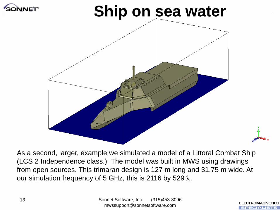
Ship on sea water


As a second, larger, example we simulated a model of a Littoral Combat Ship (LCS 2 Independence class.) The model was built in MWS using drawings from open sources. This trimaran design is 127 m long and 31.75 m wide. At our simulation frequency of 5 GHz, this is 2116 by 529 λ.

13

Patch Array Source


14

We used an 8 element linear patch array as the source radiator. The array is close to 6 wavelengths (free space) long at 5 GHz. The resulting farfield pattern is as shown above to the right. The directivity is 16.92 dBi. This simulation was carried out using the Transient solver.

We used this pattern as a source excitation on the ship.

Sea Water


15

The A-solver can use surface impedance material to approximate scattering from lossy dielectrics. The ship will be modeled on sea water replaced by a surface impedance model designed to give the proper scattering.

A 3.3 by 3.3 λ (free space) block of sea water was simulated to determine a surface impedance. The bulk properties of sea water from the CST material library are as shown.

Z-Parameters for Sea Water


16

The transient solver was used to simulate scattering from sea water. The resulting Z-parameters are as shown. At 5 GHz, we have Z = 43.32 + i8.91 ohms.

Note: This result is for the plane wave excitation normal to the surface. The off axes incidence results could differ and would need Floquet port mode simulation using the F solver.

Surface Impedance Model - Sea Water


17

We use the Z obtained in defining the material properties for the ohmic sheet surface impedance at a single frequency. A sheet of this material was placed under the ship to give scattering as from water.

Farfield Source


18

The patch array farfield pattern from the T-solver simulation were used as a farfield source in the A-solver simulation of the mounted array. The pattern was imported twice as two sources and placed at different locations.

Source Placement – Case 1


19

As the first case, the placement and the orientation of the two farfield sources are as shown. Notice that the pattern was rotated to be that of a vertical array rather than a horizontal. The distance of separation between the two antennas along the Z axis is around 125 wavelengths. The sources will be moved closer in case 2.

The idea is to excite the horizontal beams individually and then study the coupling between them.

A-Solver Parameters


20

The Asymptotic (A) solver uses the SBR technique as before. The parameters are as shown. The two farfield sources show in the source settings. We excited one of them leaving the other with zero amplitude and vice versa.

For a very electrically large structure like this one, a 5 ray density per wavelength setting is used. The observation angles are set for a full 3D farfield pattern with a resolution of 2 degrees.

Farfield - Source 1 Excitation


21

The farfield pattern for the mounted antenna is as shown. The peak directivity is similar to the source pattern. This is expected as the source is placed high on the top of the post. Scattering from the ship and water has given a pancake structure with local peaks to the pattern.

Farfield - Source 2 Excitation


22

For excitation of source 2, we can see a 3% increase in the peak directivity. This is due to reflections off the metal surfaces, edges and objects in close proximity to the source and also from the water surface.The coupling between the antennas was calculated using a macro and for case 1 was very low around -115.9 dB.

Source Placement – Case 2


23

The farfield source 2 is now moved closer to source 1 to study the change in coupling. The separation distance is now decreased to around 25 wavelengths.

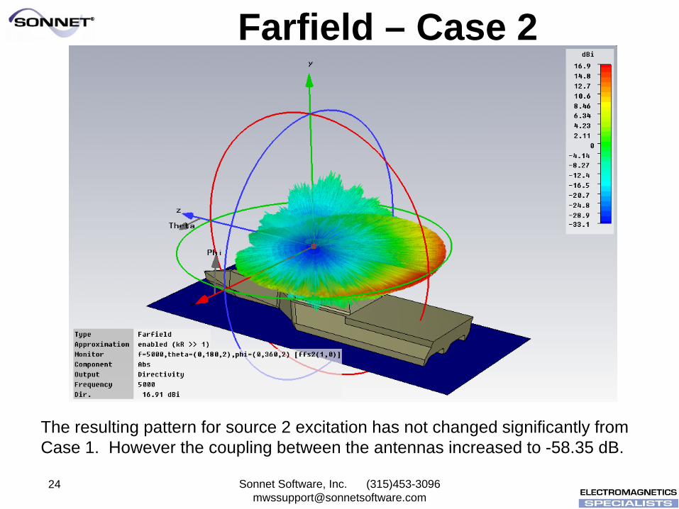
Farfield – Case 2


24

The resulting pattern for source 2 excitation has not changed significantly from Case 1. However the coupling between the antennas increased to -58.35 dB.

A-Solver Log


25

The solver log for one of the simulations of the antenna on the 2116 by 529 λ ship model is as shown above. The simulation took 18 h on an Intel dual Xeon X5550, 2.66 GHz, Nehalem architecture, 8 core machine. The peak memory used was 242 Mb.

Summary


26

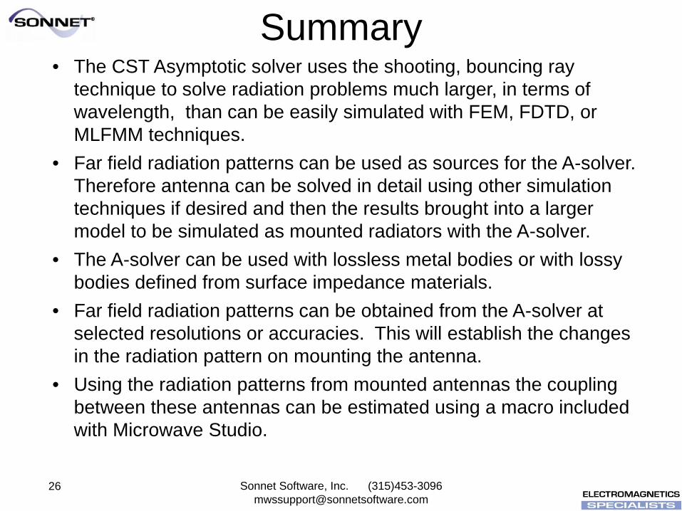
• The CST Asymptotic solver uses the shooting, bouncing ray technique to solve radiation problems much larger, in terms of wavelength, than can be easily simulated with FEM, FDTD, or MLFMM techniques.

• Far field radiation patterns can be used as sources for the A-solver. Therefore antenna can be solved in detail using other simulation techniques if desired and then the results brought into a larger model to be simulated as mounted radiators with the A-solver.

• The A-solver can be used with lossless metal bodies or with lossy bodies defined from surface impedance materials.

• Far field radiation patterns can be obtained from the A-solver at selected resolutions or accuracies. This will establish the changes in the radiation pattern on mounting the antenna.

• Using the radiation patterns from mounted antennas the coupling between these antennas can be estimated using a macro included with Microwave Studio.

antenna placement on large platforms

Documents