SOME DYNAMIC ASPECTS OF STRUCTURAL MANIPULATION

N

ANTHONY DOUGLAS HUGHES

Thesis Submitted for th Degree of

Doctor of Philosophy

-

University of Edinburgh

July 1975

:0

'p

CONTENTS

Page Number

ACKNOWLZPG$1INTS

V

SYNOPSIS VI

CHAPTER

INTRODUCTION

. 1.1. Research Motivation. 1

1.2. Existing Techniques Related to the Problem of 8

Minimising Structural Response.

1.21. Structural Optimisation. 8

1.22. &nafl Perturbation Analysis as a Method of 10

Determining the Sensitivities of EigenvaJ.is to

Parameter Changes in Dynamical Systems.

1.3. Vibration Control Using Structural Manipulation. 15

CHAPTER 2

THE EFFECT OF PARAMETER CHANGES ON THE RESPONSE OF A SINGLE

DEGREE OF FREEDCM SYSTEM

2.1. Equationsof Motion. 18

2.2 • The Variation of Frequency. 20

2.3. The Variation of Mass and Stiffness. 20

2.14.- The Variation of Damping. 22

2.5. Conclusions. 22

\ I

Contents (Continued)

Page Number

CHAPTER 3

PARAMETER CHANGES IN MULTI-DEGREE OF FREEDOM SYSTEMS

3.1. Introduction. 24

3.2. Response as a Function of a Single Variable 24

Stiffness Parameter.

3.3. Response as a Function of Two Parameters. 36

3.14. Response as a General Function of H Variable 43

Parameters.

-N

3.5. Variable Mass. 44

CHAPTER IL

THE ASSESSMENT AND EFFECT OF PARAMETER CHANGES

14.1. Introduction. 48

1.2. The Feasibility of Achieving A Desired Response 48

Using One or Two Parameters.

14.21. A Single Variable Parameter. 48

14.22. Two Variable Parameters. 51

4.3. The Criteria Governing the Effectiveness of 53

- Parameter Changes.

14.14. The Practical Application of Effectiveness Criteria 56

to a Helicopter Fuselage.

14.141. Discussion of Results. 70

14.5. Parameter Changes in Real Structures. 72

14.6. Other Techniques for Assimilating the Effectiveness 79

of Parameter Changes.

14.61. Response as a Function of Frequency and Stiffness. 79

14.62. Multiple Responses as a Function of Structural 82

'Parameters.

- II

Contents (Continued)

Page Number

CHAPTER_5

CONPUThTIONAL ANALYSIS

5.1. introduction. 88

5.2. The Structure]. Manipulation Programme. 89

5.21. General Description. 89

5.22. Programming Techniques. 98

5.3. Conclusions. 106

CHAPTER 6

EXPERIMENTAL ANALYSIS

6.1. Introduction.

6.2. The Design and Development of a Variable Stiffness •'ei

U

Element.

• 6.21. General Specification.

6.22. The flectro-Mechanicaj. Spring.

6.23. Interchangeable Spring Elements.

6.24. The Air Spring.

6.25. The Variable Length Cantilever Spring.

6.3. The Test Structure.

6-4. Erprinenta]. Equipment.

6.5. Experimental Procedure.

6.51. The Measurement of Structural Response as a

Function of Variable Stiffness.

6.52. The Measurement of Natural frequencies, Norma].

Mode Shapes and Associated Damping.

6.6. The )lathematica]. Model of the Test Structure.

6.7. Results.

- III

109

109

111

111

119

121 -

130

134

137

139

145

149

Contents (Continued)

Page Number

6.71. Natural frequencies, Norma]. Mode Shapes and 149

Associated Damping.

6.72. Response as a Function of Variable Stiffness. 164

6.8. Conclusions. 168

6.81. The Mathematical Model of the Test Structure • 168

6.82. Response as a Function of Variable Stiffness. 169

CHAPTER 7

UUNULUSIONS 170

APPENDICES 175

'N

REFERENCES 200

PUBLISHED WORK 204

F

ED

ACKNOLED&1TS

The Author wishes to thank the following: Several people at

Westland Helicopters Ltd. for their help and encouragement, Dr. G.T.S

Done for his valuable assistance and supervision, Mr.G.Smith for his

help In the construction of the experinental apparatus and to Mrs .S.M.Boyes.

and DR.W.Hughes for their superb work in the typing and preparation

of the thesis respectively. Thanks also go to Miss S.Mack for her

help in the typing of the thesis.

V

SYNOPSIS

The response of both single and multi-degree of freedom systems

is examined as a function of structural parameters. These parameters

are either the variation of mass at a structural node ox the variation

of stiffness between two points in the structure (as represented by a

linear spring). In both single and multi-degree of freedom systems

the variation of either a mass or a stiffness parameter is seen to

produce a circular response locus in the complex plane at some other

point in the structure • The form of the circular response locus is

verified experimentally by varying a single stiffness parameter in a

simple test structure • Where two or more parameters are varied

simultaneously then an area of feasible responSe is formed in the

complex plane, for any given values of the parameters the response must

lie within the bounds of this region.

The properties of the response circle and feasible response

regions, are investigated and' are used to develop criteria which enable the

relative effectiveness of parameters in achieving a desired response to

be determined. These effectiveness criteria are used in the analysis

of a simplified model of a helicopter fuselage and are shown to be

successful in highlighting sensitive areas of the fuselage for the

purpose of structural modification. An interactive computer programme

which is used to perform the above mentioned analyses on structural

models is also described.

VI

CHAPTER 1

INTRODUCTION

- 1.1. Research Motivation.

The motivation for the research presented in this thesis came

from the helicopter industry. The problem, which is a common one, concerns

the undesirable rotor induced vibration levels that often exist in a

helicopter fuselage. The design specifications for modem helicopters include

the maximum permissible vibratory acceleration levels that are allowed to

exist in certain parts of the fuselage structure; of particular importance

are the passenger and crew areas where considerable discomfort can be

experienced as a result of high levels of vibration. If this particular

specification is not achieved then modifications must be made to the structure

in order to reduce the vibratory response to an acceptable level.

The vibratory forces and moments that are inherent in the operation

of a helicopter rotor are . produced at the rotor head. These are the

resultant of loads generated on an individual' rotor blade at frequencies

which are multiples of the rotor speed. Depending on the number of rotor

blades used certain frequency components reinforce each other and others

cancel out. The most important of these non-cancelling components is

the fundamental one which occurs at a frequency which is equal to the

• . product of the number of blades and the rotor speed. The loads that are

generated at the rotor head are vertical, longitudinal, and lateral shear

forces and rolling and pitching moments • It is the response of the

airframe to these loadings that constitutes the vibratory problem of

the helicopter.

During the design process there are several aspects of the helicopter

-1-

1.1. (Continued)

design that are considered in order to ensure that vibration levels are

kept to a minimum. There are three main methods by which this may be

achieved, namely,

By reducing the vibratory force input to the fuselage.•

By the use of force cancellation devices such as dynamic

vibration absorbers.

By means of structural modifications.

In the case of the Westland Lynx helicopter method (a) was used indirectly

in an attempt to dynamically isolate the engine and main rotor gearbox

from the fuselage using flexible mountings 1211 The geometry and dynamic

characteristicsof the engine and gearbox couplings and supports were varied

in order to find the configuration that gave the smallest response at the

gearbox mounting points. In method (b) the use of vibration absorbers

is avoided wherever possible at the design stage since these often impose

a considerable weight penalty on the structure • Another method that is

commonly used, which involves structural modification, is to estimate the

natural frequencies of the structure and to determine whether any of these

are close to the major excitation frequency. Where this is the case then

structural modification is employed to move the offending frequency away from

that of the excitation forces. There are however, difficulties in this

type of approach for it is not always obvious which areas of the airframe

are most suitable for structural modification. Thus there is the real

need to be able to predict accurately the effect of structural modifications

on the response at points in the airframe.

Even though efforts are made during the design stage of the helicopter

to reduce vibration levels it is often found when the helicopter is first

flight tested that these are still unacceptable and there is usually

—2-

t

1.1. (Continued)

considerable pressure on the dynamicists involved to come up with a

satisfactory solution to the problem. At this stage tha'e are two main

methods of reducing undesirable vibration levels, namely, by using

vibration absorbers and by structural modification.

In the first instance structural modification is often used to

help solve the problem. A series of potentially useful modifications is

drawn up and each modification is tried in turn, under flight conditions,

in order to determine how effective it is in reducing the required

vibration levels. Where a particular modification is found to be

successful then it is incorporated into the existing structure. Most

modifications involve stiffening up the structure in some way and are

chosen largely on the basis of experience and intuition. The choices are

sometimes influenced by results from an analysis of a simplified model

of the helicopter; the model used in the case of the Lynx helicopter is

described in Chapter Ii.

Having modified the structure to the beat effect by incorporating

certain modifications the vibratory response may be further reduced by

means of dynamic vibration absorbers.. These may be used to suppress

vibration globally with respect to the fuselage itself or locally at

specified points in the structure. The simplest vibration absorber consists

of a man, spring, dashpot system which is timed to resonate at the

excitation frequency of the structure • This type of absorber is usually

mounted close to the point at which the vibration level is to be reduced

and is intended to suppress vibration only on a local basis. In

practice the mass in such a device is usually an existing piece of heavy

equipment such as a battery; an example of a battery absorber is shown in

figure 1.1. (a). Other types of absorber, which suppress vibration globally,

—3-

roui iituu

[B]

Bifilar Pendulum Absorbers

Dynamic Vibration Absorbers

Figure 1.1. —4—

centre spring

..J I-/v'1. '

assembly [Al Battery vibration absorber

pendulum

1.1. (continued)

are norm" situated close to the source of excitation. Typical

examples of these include the bifilar pendulum absorber,DAVI absorbers

and the Bell "Nodanagic" system.

The bif liar pendulum absorber was first used to reduce torsional

vibration in an engine crankshaft. [221 Where the helicopter is

concerned, a set of bifilar absorbers is fitted in the plane of the

rotor head as sham in figure 1.1. (i,) and is effective In reducing

forces in that plane. The absorber consists of a large mass which

acts as the pendulum bob, and is mounted at the end of a very small

radius arm. Unlike some types of absorber,'.once the pendula have

been tuned to a given frequency then they remain in tune even if

the frequency changes. This is due to the fact that the dynamic

stiffness of the pendulum, as provided by the centrifugal force, increases

or decreases with a similar change in the rotor frequency.. The bifilar

absorber has been successfully applied in practice to production

helicopters by the Sikorsky Aircraft Company [231,

The Dynamic Anti-Resonant Vibration Isolation System (DAVI) was

patented by the Karman Aircraft Corporation and consists of the

mass, spring arrangement shown schematically in figure 1.2. (a). The

system is tuned to the excitation frequency such that the mass A resonates

on the end of the rigid bar. In any practical application the engine

and main rotor gearbox would most likely be mounted on a set oZ absorbers

in an attempt to isolate this substructure from the rest of the fuselage.

• DAVI absorbers are at Present still in an experimental form and have

not been applied in a practical situation.

A similar arrangement to the DAVI absorber is the Bell 5Nodamagio"

system shown in figure 1.2. (b). The main rotor gearbox is mounted

-5-

excitation force

gearbox engine etc

EA --- 1 )

spring /\

fuselage

[A]

DAVI Vibration Absorber

F -

gearbox mounting struts

eLastomeric bearing

¶ etastomeric sandwich (rubber & steel)

• airframe1

[B]

Belt 'Nodamèigic" Gearbox Mountinq..$ystem

Dynamic Vibration Absorbers.

Jigure 1 .2 —6— •

1.1. (Continued)

on a beam supported by elastomeric bearings. The beam and carried mass

are tuned to resonate in the first "free-free normal mode of the beam

at the external excitation frequency. The beam supports are positioned

to coincide with the nodes of the normal mode in an attempt to minimise

any forces transmitted to the airframe.

• N Dynamic absorbers are essentially force cancellation devices and

are often very effective in reducing vibratory responses. Their main

disadvantage, however, is that they often impose a considerable weight

penalty on the structure, e.g. the bifilar can add as much as 14 to the

total weight of the helicopter. Battery absorbers and other similar

devices, with the exception of the bifilar, also have to be tuned to a

given frequency in order to operate in an optimum manner. The rotor

speed, which is governed, can vary in certain circumstances by a small

amount and if this does happen then the excitation frequency changes and

the absorber becomes detuned and is consequently not so effective.

It is evident that whenever a structural modification has to be

made, tether it is at the design stage of the helicopter or during the

flight test trials, then there is always the problem of identifying those

areas of the structure that have the greatest potential in either affecting

or reducing the desired vibratory responses. Thus although the primary

aim of any investigation using structural modification would be to reduce

to a minimum the vibration levels in selected areas of the helicopter

fuselage, there are two secondary aims of a more general nature. Firstly,

there is the need to develop techniques which will give a better understanding

• • of the way in which the dynamic response of a complex structure varies as

a function of its structural parameters, and secondly, criteria must be

—7-

1.1. (Continued)

developed which will highlight areas within the structure which are

potentially effective in reducing the desired vibration levels.

1.2. Existing Techniques Related to the Problem of Minimising Structural

Response.

1.21. Structural Optimisation.

Computer bases formal optimisation routines are ccmun-orty used

in the Aerospace industry in a wide variety of applications. A general

optimisation procedure contains an objective function,variables and

a set of constraints which may be ap plied to the parameters themselves

or which may be of an independent nature such as stiffness or frequency

requirements. Typically, an optimisation procedure can. be apj,lied to a

finite element model of a complex structure in order to achieve a

minimum weight configuration. The structure would normally be subjected

to a set of excitation foi'ces and the variables in the problem would be

the sizes of the elements. The constraints could include any of the

following: stress constraints, constraints on the displacements and also

on the sizes of the elements. An example of a procedure such as this

is given by Venlcayya 1251

Dynamic constraints can be considered in the optimisation process,

e.g. it might be required that one or more of the natural frequencies -

of the structure should assume given values or alternatively that there

should be a given interval between io natural frequencies.. Turner 26

develops a procedure which proportions the members of an elastic structure

so that- one or more of its natural frequencies assumes a given value

and the total mass of the strucure is a minimum. Constraints of this

form are normally considered in order to satisfy the flutter requirements

!\ of fixed wing aircraft.

-8-

1.21. (Continued)

A particularly practical method has been developed by Taig and

Kerr (29) at the British Aircraft Corporation where automated optimisation

methods are routinely used in the design of all new aircraft. The

method is capable of producing a minimum weight structure whilst considering

strength, stiffness and frequency requirements simultaneously. The

approach is based on the strain energy- density of individual structural

elements and all the above mentioned requirements are developed in terms

of these. The variables considered in the process are real structural

painters and there is consequently no need to perform a subsequent design

operation in order to convert idealised structure dimensions to feasible I

detail sizes.

The problem of minimising structural response can be tackled using

formal optimisation techniques. The method requires a mathematicsl

model of the structure in order to calculate the dynamic response of the

system due to a given set of excitation forces • The response at one

or more points in the structure is minimised as a function of a given set

of structural parameters. Constraints can be imposed on the sizes of

the parameters as in the previous problems. Ellis (27) of Westland

BelicoptersLtd., describes a process by which a very much simplified model

of the upper decking structure, main gear box and engine of a helicopter

was optimised in order that theforce inputs to the fuselage were a

nixthnum. The problem contained only a few variable parameters representing

the geometry and stiffness of the substructure • A Simplex procedure was

used in the optimisation routine and the results obtained were used in

order to obtain a feel for the vibration problem of the helicopter. An

attempt was subsequently made to optimise a simple model of the whole

helicopter containing 20 nodes and 25 linearly tapered beam elements.

—9-

1.21. (Continued)

In this particular case it was required to minimise the response in

the area of the pilot's seat subject to variations in the flexibility

of elements in the engine-gearbox area. It was found that the

procedure required approximately 1126 hours of C .P .0 • time for one

computer run and the idea was consequently abandoned.

The results of the latter application demonstrate quite clearly

one of the main disadvantages of formal optimisation procedures. It

is apparent that in large structures there are often many thousands

of parameters and to consider each of these as variab)Ds in an

optimisaticn process would be beyond the scope of even the largest and

most efficient of modern day computers. A reduced selection of the

most likely parameters would therefore have to be chosen as the variables

in the problem. However, this approach is not entirely satisfactory

for there is no way of knowing whether the minimum solution achieved

is a global, minimum or just a local me, i.e. could a better solution

have been achieved using a different set of parameters? The results from

an optimisation process also give no indication as to the relative

effectiveness of given parameters for the purpose of achieving a minimum

solution, and by virtue of the predetermined way in which the search

for this minimum is carried out the process effectively lacks the freedom

which enables any sort of feel or insight into the problem to be obtained.

1.22. Small Perturbation Analysis as a Method of Determining the

Sensitivity of Eigenvalues to Parameter Changes in Dynamical

Systems.

The three methods outlined in this section can be used in an

indirect manner to assess the effect of structural modifications on the

dynamic response of a system. The methods attempt in one way or another

to determine the sensitivity of eigenvalues to changes in certain

-10-

1.22. (Continued)

parameters of the system. It is assumed that if any close natural

frequencies of the system can be moved away from the excitation frequency

then this will result in a reduction of the totsl dynamic response of

the system due to the contributions of the associated

normal modes • Of the three methods examined only those of Sciarra are

aimed directly at the reduction of structural response • The methods of

Newman and Simpson are of a more academic nature and are aimed more

specifically at the problem of flutter in aircraft lifting surfaces.

The Methods of Sciarra. [16,17,18]

Sciarra considers the problem of reducing the dynamic response

of a helicopter fuselage directly. Two distinct approaches are used,

namely, dynamic vibration absorption and structural modification.

Vibration Absorbers.

A technique is developed that will predict the effect on

structural response of introducing dynamic vibration absorbers into

the s,,rstem. The amount by which the vibration levels can be reduced at

specified points in the structure is calculated and is used as a measure

of the effectiveness of the absorber. Where more than one absorber is

used then Sciarra, shows that it is sometimes necessary to detime one or

more of them in order to achieve the optimum reduction in vibratory

response. Because of the weight penalty incurred by using vibration

absorbers this approach is usually only used after an attempt has been

made at structural modification.

Structural Modification.

In the second approach it is assumed that if the natural

frequencies of the structure are moved away from the excitation

frequency then this will result in a general lowering of the dynamic

1.22. (Continued)

response of the system. The problem thus rethees to one of assessing

the effect of changes in structural parameters on particular natural

frequencies of the system. The effectiveness of parameters is based

on the strain energy of indivIdual structural elements. In the first

instance a finite element analysis is performed to yield the eigenvalues

and eigenvectors of the system, then the modal strain energy distribution

throughout the structure is found for the mode shape whose natural

frequency is to be modified. The strain energies of each structural

element are calculated and listed in descending order, those elements

with the highest values are considered the best candidates for

modification of the natural frequency. An alternative method of

calculating the strain energies using the damped forced response in

place of the mode shape is also mentioned. Sciarra points out that

the procedure can be made more optimal from the point of view of

minimising weight by considering strain energy densities rather than strain

energy alone. U

This technique is useful in that it indicates the potentially

effective elements for the purpose of structural modification. The use

of strain energy as an effectiveness criterion is seen to be relevant

in as much that vibration levels were reduced using the suggested

nodificationsj. the method, however, doesrnt give any direct Indication

• as to the magnitude of the parameter changes that would be required.

• One way of resizing structural elements [301is given as •

t . (X (strain energy density of the element)

(max strain energy density of any element).

where At is the change in the parameter (area, thickness, moment of inrtia)

and Of is an arbitrary constant which represents the mnrlmmn allowable weight

—12-

1.22. (Continued)

penalty. It is not however, obvious whether the magnitude of the

parameter change chosenin this way will produce the optimum reduction

in vibration levels. The process by which real s'uctural parameters

are used to reduce the dynamic response is involved and contains

several assumptions; the flow diagram shown in figure 1.3. represents

this process.

The Bouts by which Structural 'Response is Affected by Changes in a

Structural Parameter.

Figure 1.3.

The Method of Newman

This method is aimed specifically at the problem of flutter of

aircraft lifting surfaces, although the analysis could be applied to the

equations of motion of any linear dynamical system. The technique

involves the reduction of the general equations of motion of an N

degree of freedom system to a set of first order differential equations of

the form 9

.* * a

Where i =

and

—13-.

1.22. (Continued)

Si. being the generalised coordinates of the system and N is a (2n x 2n)

matrix whose elements are functions of the system matrices such as mass,

stiffness and damping. If X are the eignevalues of N then the

method sets out to determine the rate of change of A i with the

individual elements of M. i.e. to find d1 This derivative is — dmJkth

ref ered. to as the condition number for the jk element of H with respect

to the ith eigenvalue. Those elements with the largest condition

numbers are considered to be the ones to which the eigenvalue is most

sensitive.

The method can thus be used to identify the potentially effective

elements for the purpose of altering a given eigenvalue. However,

any change in a real structural parameter usually affects more than

one element of matrix N which may result in an undesirable effect on

the eigenvalue under consideration. For the same reasons the reverse

process of relating an element m ij to any given parameter is

complex, and consequently it is most likely that considerable difficulties

would be experienced should this method be applied to a practical

problem.

A method similar to that of Newman is given by Woodcock L".

The method is used to calculate the eigenvalue sensitivities, only this

time they are obtained without having to reduce the equations of motion

•

of the system to a set of first order differentials.

The Method of Simpson 2

• In this method the sensitivities of eigenvalues to changes in

structural parameters are determined using techniques suggested by

Kron 1201 for the iOlutioñ' of large scale eigenvaluO problems. Krcn 'a

method;' eAn 15ealied to the Sólut.lbn of eigenvIiid Problems which

• \ an tod large for a given comj,utei'to handle. 'hid chiuhi.equires

• Ii

- • —14-

1.22. (continued)

that the composite system be split into N subsystems, for each of

which the eigenvalixas. may be extracted easily. The equations of

motion of the composite system are derived by recourse to the concept

of a constrained primitive Lagrangian followed by an application of

Hamilton's principle. An "Intersection Lambda " matrix is derived

• whose order is small compared with that of the composite system. The

eigenvalues of this matrix are identical to those of the composition

system and can be extracted quite easily.

• Simpson considers a change in a structural parameter S in

one of the subsystems and develops an expression for the eigenvalua

sensitivitydA; an expression for the eigenvectornsitivities is

also developed. The method provides useful information concerning

the sensitivities of eigenvaluesdirectly in terms of real structural

parameters, and unlike the methods of Newman and Woodcock the procedure

is not further complicated if a structural parameter affects more than

one element of the mass or stiffness matrices.

• The methods of Newman, Simpson and Woodàock are very much of an

academic nature and would probably contain serious limitations when

applied to a truely practical problem. The method of Sciarrayon the

other hand, has been developed from a practical view point and has been

proved successful in its application.

• 1.3. Vibration control Using Structural Manipulation.

The theory develped in this thesis is based on a little known 1 131 property of linear structures that was first noticed by Vincent

of Westland HelicoptersLtd. If a structure is excited by a single

• • sinusiodal force whilst either mass at a point or the stiffness

between two points (as represented by a linear spring ) is

—15-

1.3. (Continued)

continuously varied then the response in the complex plane at some other

point is seen to trace out a circular 1oct12 • This simple yet elegant

result forms the basis for all the subsequent analysis that is developed.

By way of an introduction to this approach the response of

a single degree of freedom system is determined as a function of mass,

stiffness and damping. The variation of all three of these parameters

is seen to produce a circular locus. Throughout the analysis

structural response is given in terms of receptances, i.e. response

per unit force • The theory is extended to cover the case of

parameter variations in multi-degree of freedom systems. For the variation

of a single mass or stiffness parameter the simple circular locus is

shown to exist, However, where two parameters are varied simultaneously

an area of "feasible response" is found in the complex plane and for any

given values of the two chosen parameters the resultant response must

lie within the bounds of the feasible region. It will be shown that

it is possible to determine whether a desired response is feasible or

not for any given combination of parameters. A general matrix equation

for the response as a function of K variable parameters is also

developed.

With reference to the practical application of this theory, -

criteria are developed for the purpose of assessing the effectiveness

or sensitivity of parameters; several of the properties of response

circles and feasible response regions are incorporated in these • The

criteria' can be used to determine areas of a structure which are

potentially effective in reducing vibration levels. The practical

application of the theory is demonstrated using a simplified model of

a helicopter fuselage. The analysis is undertaken in order to

1.3. (Continued)

highlight sensitive areas of the fuselage for structural modification

in order to reduce vibration levels in the passenger and crew areas.

The results are compared with those obtained from a practical analysis.

An experimental analysis is undertaken to verify the form of the

circular response locus as a function of variable stiffness • The

analysis is performed on a simple test structure in which the stiffness

of a linear spring element is varied. The results obtained are

compared with those predicted theoretically..

An interactive computer program is developed for the purpose of

testing the theory. The program is used as an aid to the research

process and also as a means of performing practical analyses on

structures containing up to 60 degrees of freedom.

The methods outlined in the following chapters form the basis

for a completely new approach to the problem of vibration reduction

by means of structural modification. The method is intended to give a

better understanding and also a "feel" for the problem, both of which

are lacking in existing techniques.

p.- -

—17-

CHAPTER 2

THE EFFECT OF PARAMETER CHANGES ON TI RESPONSE OF

A SINGLE DEGREE OF FREEDOM SYSTEM

2.1. Equations of Motion.

Although possibly of little practical importance, a brief

study of the various parameter changes in a simple one degree of

freedom system is helpful in understanding similar changes in more

complicated cases. It is intended to show how the response of the

system varies with frequency, mass, stiffness and damping.

The equations of notion of a single degree of freedom system

subject to harmonic excitation at circular frequency may be written

jj+ +kx" Fet

where m is the mass, Ic the stiffness and F the magnitude of the

excitation. The daiüping, represented by constant h, is considered

to be hysteretic in the analysis that foflows. The steady state'

solution for the response is given by

1 - G(Q)Fe t

where

0(1.4 - 1

(k - mc)) + iii (2.3)

and is the complex receptance of the pystem. Since the receptance

is the response per unit magnitude of excitation, it is this quantity

that is considered in the ensuing analysis rather than the response

itself.

—is-

I- I

Inc recising

The Response of a Single Degree of Freedom System

as a Function of frequency

3(w)

Figure 2.1. —19—

2.2. The Variation of Frequen cy.

The results of varying frequency are well known and so need

only be considered briefly. It can be shown that the locus of the

tip 01 the receptance vector G(Lo) in the complex plane, astavaries,

is a circle diameter 1/h passing through the origin and centre on the

negative imaginary axis . Figure 2.1. shows the circle as a

projection of the three dimensional locus produced by including c.s

as the vertical coordinate. The complete circle can only be realised

by considering imaginary values ofwi.e. w 2 c 0 (shown dotted in the

figure). Various points of interest, including the direction in

which the circle is traced out for increasing values of a, are also

shown.

2.3. The Variation of Mass and Stiffness.

The circular locus described in section 2.2. arises by virtue

of the variation in the real part of the denominator (k - mL3 2 ) in

equation 2.3. Thus, it may be seen that a variation in m or k

produces the same locus. For increasing values of Ic the direction in II

which the locus is traced out (anti-clockwise) is opposite to that for

• increasing values of in and ,,2. Arcs corresponding to negative values

of in and k exist in a manner similar to that for w2< 0. Listed

below are the coordinates in the complex plane corresponding to some

of the more important values of in, Ic and w.

to, 01

1 k1 (0 +h2 ),_W(k2 +h2 )1 k - o [-mu 2/(iAJ' + h2 ), -h/(ntF+ h2 )]

If the circles for G(k) are plotted in three dimensions for all values

of o, a circular cylindrical envelope is developed. Figure 2.2.

Shows a pictorial representation of this.

-20-

'a

Ii

Increasing k

Response as a Function of Stiffness and Frequency

(One Degree of Freedcvt)

0(k)

Figure. 2.2. -21-

2.3. (Continued)

Those parts of the loci corresponding to negative values of

It are shown as dotted lines. In addition it is possible to plot, on

the envelope, curves of constant k; these are of the same type as

those shown in Figure 2.1.

2.4. The Variation of Damping.

Varying the damping coefficient h in equation 2.3. produces a

circular locus diameter k/(k - m(42 ) with its centre on the real axis

and passing through the origin .ltere &O/iE the circle lies on the 'In

positive real axis (forocfiZ on the negative real axis) and the locus 'in

is traced out in an anti-clockwise direction for increasing values

of h (for wcJi? the direction is clockwise).

In practice inherent damping in a structure is a difficult

quantity to model precisely and it is not envisaged that parameter

changes of this form would be used to alter the structural charact-

eristics. Consequently, the effects of changes in structural damping

are not considered further in this analysis.

2.5. Conclusions.

It has been demonstrated that the independent variation of ax

of the parameters in a single degree of freedom system produces a simple

circular locus in the complex plane. When an increase or decrease in

stiffness is accompanied by a similar change in the mass, as is often

the case In practice, a variation in one parameter tends to cancel

out the effect of a change in the other; but clearly combinations of

parazieter changes do not further complicate the analysis.

It will be shown in Chapter 3 that the simple form of the

circular locus carries over to systems with many degrees of freedom,

-22-

for varying mass and stiffness, but not for varying frequency.

N

- -23-

CHAPTER 3 N

PARAMETER CHANGES IN MULTI-DEGREE OF FREEDG1 SYSTEMS

3.1. Introduction.

The general case of an N degree of freedom system subjected

to a single point excitation is considered. The response at any

point in the structure is examined and the main properties are

developed for the case of varying stiffness. At the end at the

section varying mass is considered, and is seen to produce a response

locus of the same type as that obtained for varying stiffness. The

complete development of the theory for variable mass is shown to be un-

necessary since, by implication, the properties and observations for

this are similar to those appertaining to variable stiffness. A simple

analogy is made between variable mass as a parameter and a special

case of variable stiffness. In this way it is possible to use just

one set of equations to describe the response at a point in a structure

as a function of mass, stiffness or mixed parameters.

The effect on the response is examined for the variation of

o, two and H stiffness parameters. Having developed the theory,

certain facts and observations are made within the analysis; some -

information is given only on the grounds that it is interesting, whilst

a fuller treatment and discussion of the application of the theory is

given In Chapter U.

3.2.. Response as a Function of a Single Variable Stiffness

Parameter.

i.e in the single degree of freedom case, the response of the

system is expressed in terms of receptances. The latter follow from

-24-

3.2. (Continued)

consideration of the equations of motion of an N degree of

freedom system which may be written .. lot - fl+C+KiFe (3.1)

where N, C and K are the mass, damping and stiffness matrices

respectively. The system is considered to be subject to harmonic

excitation at circular frequencyto and, since no further advantage.

may be gained from using hysteretic damping, the damping is considered

to be viscous. The steady state solution for the response is given

by

- iL.t -. x xe

where

x, = GF (3.3)

and G =[K-Mt. + aCt.] 3.

which is the receptance matrix for the system. Figure 3.1. shows

schematically the system to which the equations apply. It represents

a structure having many degrees of freedom, for which it is required to

examine the response at a material point q due to a single forced

excitation at point p. The structure is modified by inserting a

linear spring of stiffness It between points r and a having mutually

compatible degrees of freedom. The spring is adjusted so as to exert

zero force when the system is iii equilibrium.

-25-.

0

)

Figure 3.1.

Schematic Representation of the Structure and Variable Stiffness Element

Considering the original structure as a free body, the

introduced spring exerts forces Fr and F9 at points r and a respect- .

ively., where

!r. k(x3 _Xr) - -F3 (3.5)

This gives a relationship between the parameter Ic and the, structural

variables of force and diaplacemnt. Equation 3.5 thus provides a

rigorous definition of the form of the parameter change where stiffness

is concerned. The forcing vector F in equation 3.3 now contains three

non-zero elements F1 Fr and F5 , the latter two being dependent on the

structnrai. displacements x and x 0 9 tlst the elements of immediate

-26-

3.2. (Continued)

interest in the displacement vector A are x x and x5 . By

partitioning and expending the relevant parts of equation 3.3. we can

write

q qpp qr F r qas

x -G F +G F +0 F r rpp rrr rae

x = G F +0? +G F s app err ass

(3.6)

Where G is the complex receptance giving the displacement at point iii unit

due to akforce at point J. The forcing terms Fr and F may be

substituted from equation 3.5. and subsequent elimination of Zr SM

in equation 3.6. gives

xq - 0qp + Ic (0 Si, - a

I'p )(Gqr - cas (3.7.)

F P rr l+k(G +0as ra sr -G -G )

This is now the modified complex receptance between points p and q in

terms of the variable parameter Ic and the original receptances

Equation 3.7. may be written in the more general form

oCu+iv

- (e+ if) +Ic(a+ib) (3.8)

l+Ic(c+id)

where DC- and a, b, c, d, e and f are all real constants.

Now from equation 3.8.

(u-e)+L(v-f)- a+ib

+ C + Id

• and r arranging this gives

E]J+c+id-(a+ib):[(u-e)-1i(v-r)I

(uJe)2 +(v - f)2

-27-

3.2. (Continued)

then equating the imaginary parts and thus eliminating k leads

to the equation

dj(u-e)2 +(v-f)2 1 b(u-e)-a(vf)

which on simplifying gives

[u- (e+b/2d)] 2 +

2 2 -a +b

[v - (f - a/2d)j 3..

which is the equation of a circle radius I a2 + d2 and centre Is + b/2d, £ - a/2d1

Thus, ask varies between - oo and +oo the locus of the tip of the

receptance vector CC traces out a circle in the complex plane. It is

interesting to note that equation 3.8. may be regarded as providing a

mapping from the k plane, which is in general complex, to the *4 plane.

This may be seen to be an example of the bilinear class of mappings

• represented by the general equation

walc+b

ck+d

where a,b, c and d are complex constants and for which it is knwn

that circles and straight lines ( a circle with infinite radius) in the

• k plane map into circles or straight lines in the '.) plane. In

this case we consider only real values of k, providing a straight line in

the k plane, which maps into a circle in the plane. If damping were

incorporated into the stiffness by introducing an imaginary component

into the parameter k, then, provided that both real and imaginary parts

can be plotted on a straight lire, the mapping on to the K plane is

still a circle.

The geometric propertis of the response circle in the PC plane

-2

3.2. (Continued)

depend on the constants a, b, c, d, e and £ which in turn depend

indirectly on the exaninaticn and forcing points and on the position

of the introduced spring. Appendix A contains a table relating

these constants to the ccmplex receptances G.

Equation 3.7. has been derived for the case where pqrgo.

However, it is possible to consider conditions other than these, and

listed below are the results for the combinations of p, q, r and a

encountered in practice.

porqrors. It can be shown that

equation 3.7 still applies with the relevant

subscripts interchanged.

p - q - rors. The subscripts may be

interchanged as in case (1).

ror a - o. This can be interpreted as

indicating that the introduced spring has

one of its ends anchored to a ground -

reference point as shown below.

-

I k Er 0 'structure Xr

-29-

3.2. (Continued)

In this ease

F-kx1.

and expanding equation 3.3. as before we obtain

x - 0 +Jc(-Q ) q 03)+

3) rp 0 qr (3,9)

F l+kG 1'l'

This result may be obtained directly from equation 3.7. by considering

the subscript a to be zero, with the condition that 0 where i

or j - 0. Thus, a zero subscript may be taken as referring to a

rigid point for which the cross receptance between this and any other

point is zero. It can now be seen that one equation, namely equation 3.7.

• can be used for all possible values and combinations of p, q, r and a.

In the latter half of this section some of the more important

• properties of response circles are examined with a view to obtaining a

• better understanding of how a particular parameter change affects the

• response of the system.

• In equation 3.8. the complex receptace t&- may be

split into its real and imaginary components which are

'u- e + k [a + k(ac + : (3.10)

1+2cic'+k2 (c2 +d2 ) -

v -f+k [(b+rc(bc- ad) ] (3.11)

1+2ck+k2 (c2 +d2 )

These equations lead to, the coordinates of two important

points on the response circle, namely those at which It - 0 and Ic -00;

substituting these values in equations 3.10. and 3.3.1. gives

[e,fJ

H

3.2. (continued)

k_OQ .....Ie+ac+bd, f+bc - ad

L It is these two points which bound the are of the circle

corresponding to negative values of k. There are, however, two arcs

to choose from, and it is necessary to determine the direction in which

the locus is traced out for increasing values of Ic before azy- decision

can be made.

m cc (k)

I Lt. -S

Re (k)

----negative k

S

I Figure 3.2.

Response Circle for Varying Stiffness

—31-

3.2. (Continued)

Figure 3.2. represents a typical response circle and 1 e defines

the angle between its horizontal diameter and any other point cones-

potiding to a given value of Ic. From equation 3.10. and equation 3.11.

G can be obtained as a function of Ic and may be written

a T/2 + Tan- 5 d-] ' _ 2 Tai [PZ-o,]

(3.12)

The constant d in the second term in the above equation is not cancelled

since its sign plays a significant part in determining the quadrant

in which the angle & lies. In order to determine whether G is an

increasing or decreasing function of k, it is necessary to calculate

dG from equation 3.12. Thus, by differentiating with respect to Ic, dk

we obtain

dG -2d

(3.13)

M. (1 + ck)2 + d2k2

from which it can be seen that the locus travels in an anti-clockwise

direction for the negative values of the constant d that invariably

occur in practice. In addition to this, it is interesting to note

that the point at which L is a maximum, i.e. dk

k -c

2 2 C

is displaced by 900 round the circle from the point at which dG

is a minimum (in fact zero, occuring at Ic a a)). The rate of change of

9- with Ic is a useful quantity in that it bears a direct relationship

to the ability of any given parameter to change the response of the

system. This property can be seen from equation 3.13. to depend

only on the position of the introduced swing and not on the examination

and forcing points q and p. Equation 3.12. can be rearranged to

-32-' Ii

II

S

3.2. (Continued)

give k as a function of S i.e.

Ic tan d - a tan p

where

P [ - . 9

2 2

This is an extremely useful equation, particularly in the computationsl

side of the analysis where it is often necessary to calculate the

stiffness value corresponding to a given response.

At the begining of this section, it was assumed that the

stiffness parameter Ic was real. However, the implication of this on

the bounded nature of the response is not immediately obvious • In

order to clarify this point, consider equation 3.10. with the constant

e omitted for convenience

• U. -. k[a+k (so +bd)] (3.14)

• 1 + 2ck + k2 (c2 + d2 )

This gives the real coordinate of the response as a function of Ic.

Equation 3.11. may now be rearranged to give a quadratic in Ic which is k [u(c2 +ct2 )- (so +bd)J +Ic (2cu.- a)+u (3.13)

no -

Solving this equation for Ic yields two roots for any given value of

w., and if these roots are to be real, as is the requirement in

practice, I then the following condition must be satisfied

4 u 2d2 -4 ubd-a2 <0 (3.16)

By considering the limiting case where equation 3.16. is zero and

solving for u , then

3.2. (Continued)

- b; v'a2+b2

2d

which corresponds to the real coordinate for the centre of the

response circle plus or minus its radius. The imaginary component

for the response given by equation 3.11. may be analysed in exactly

the same manner, and is found to yield the result that

-a %/a2+b2

2d

for the condition that k is real. When these two observations are

taken together, the implication is that there are finite limits imposed

on the maximum and minimum size of the receptance vector owing to the

real nature of the parameter Xc.

As with the single degree of freedom case (see Figure 2.2.)

it is possible, by introducing the forcing frequency to as a coordinate,

to construct a surface corresponding to a given stiffness parameter

upon which three dimensional response curves can be drawn for various

values of that parameter. Figure 3.3. shows a pictorial representation

of a typical surface, the response curve corresponding to k - 0 (shown

dotted) is projected below on to the complex plane. The latter is

often referred to as the Kennedy-Pancu plot for the system. - I

In the last half of this section, consideration has been

given to some of the properties of response circles in the complex plane.

In Chapter b these will be expanded and discussed in more detail,

•

and a description will be given of hat these principles can be applied

to practical examples

k)

3.3. Response as a Function of Two Parameters.

As in Section 3.2., the response at point q, on the

structure, due to a force at point p, is sought. This time the

variable stiffness elements k, and k are connected between points

r, a and t, v respectively. The forces r' F9 , 7 and F,, are given

by

F - ICl (x s - x r ) a

- F (3.17)

Fta Ic2 (x,,- :xt) F V

Equations 3.3. can again be used to give the relevant equations

- G1 F J i q, r, s, t, v (3.16)

jp,q,r,s,t,v

substituting for Fr 't and F, in equations 3.16. and eliminating

Zrs xs I x and x gives

-Gqp + k1 Ø 1 (Ic2 ) + Ø 2 (k2 ) (3.19)

F Ic,1 03 (k2 ) +

where 0 i T 2 are complex linear functions of k and are given in

fun in Appendix B. In order to understand how the locus of

in equation 3.19. appears on the complex plane as Ic,1 and Ic2 vary

simultaneous)yit is necessary to examine how the function behaves

when one parameter varies and the other is held constant. If, for

instance, Ic1 is held constant whilst Ic1 is allowed to vary then it can

be seen that equation 3.19 provides a mapping of the same type. as that

given in equation 3.7., i.e. it results in a circular locus. If Ic 1

assumes a different value then another circular locus is produced as

varies. If all possible values of ICc are considered then the

correspcziding k..2 loci lie on the circular locus for the system when IC1.

2

33. (Continued)

alone In varying. This is illustrated in Figure 3.14.

AIm(kk) 1 12

Re I

- - Figure 3.14.

Response Circles for Two 'Structural Parameters

—37-

33. (continued)

By considering all possible combinations of k, and k 2 , a

region in the complex plane is formed, inside which the response at point

q due to an oscillatory force at point p must lie. This is referred to

as a "Feasible 'Response Region". Figure 3.5. shows an example produced

In the same manner as indicated In Figure 3.4.

/

-

T -_- -- tIfl.

Feasible Response Region made up of Response Circles.

Figure 3.5. —39—

3.3. (Continued)

On examination the region appears to have two boundaries

and is doubly covered, i.e. a given response may be achieved using

either of two pairs of values of Ic1 and k 2 . The bouud&'ies, however,

do not exhibit this property, for it may be deduced from the graphfral

construction that on av boundary the circles for Ic1 and Ic2 intersect

at a tangent. Thus, there can only exist one pair of values Of kls

1c2 for each point on the boundary. These facts may now be obtained

in a more rigorous fashion. Mathematically the boundaries are given

when the Jacobia

6 (u,v)/b(1c1,k2 )

is zero [6] i.e.

b SIc1 k2

-O

Ax

or, alternatively -

In Dkl

_ oc] -O (3.20).

èk2 J

where is the complex conjugate of . and 5k2

cC- u +iv=5 -

F.

Equation 3.20 is of second order in Ic1 and Ic2 , thus confirming the

possible existence of two boundaries. By virtue of the fact that the

values of kj and Ic2 on these boundaries are uniquely defined it is

possible to calculate their coordinates directly. Substituting a

—40-

3.3. (Continued) I

range of values for Ic1 into equation 3.20. (see Appendix C for expanded

version of this equation) the two corresponding values of k 2 (one for

each boundary) and hence the coordinates of that point may be calculated.

By choosing enough values of Ic1 the boundaries may be plotted direotlyk

Figure 3.6. shows some examples of typical Feasible Regions. The

system for which these were calculated is described in Appendix B.

- —41-

T__AI t

('4

The Boundaries of Some Typical Feasible Response Regions.

• - •

Figure 3.6. • • -42-

I

3.1. Response as a General Function of H Variable parameters.

In Section 3.3. the setting up and reduction of equations

3.6. to give a single expression for the complex receptance in

equation 3.7. becomes rapidly more complex as the number of variables

considered increases. As a consequence of this a general matrix

expression for the complex receptance, in terms of H variable parameters,

is developed.

The response at the examination point q may be written in

terms of the external, force, internal, spring force and the corresponding

receptances Gij

x q -Q qp

p p 6 1 q1 - q2 + 1c2rS2 (Qq - Gq ) ;

,.,q. k5 (Gq 2m-1 - Gqi ) (3.21)

where k is the ivariable stiffness parameter and

X - i 2± X2i_1

is the extension of the ith spring ( x2i and X2j1 being the actual

displacement at each end). Equation 3.21. may be alternatively.

expressed

xq qp p U F +AK.6 (3.22) -

where sisa(lxm)row vector ofterms

[(Gql - Gq2)I (G q3 - Gq) ......q,2m1 - %, 2m

is the d Km. diagonal matrix of stiffness parameters Ic 1,, and S

is a Cm x 1) column vector of extensions.

The values of , may thpmselves be expressed in the same way

as A in equation 3.22.

- °l -Si ' I(G22- U21) - - an )] - (G12

S 2 24 - 23) - (G117 U13 )]

-43-

3.4. (Continued)

6 2 - F (% - G3P 81 - k. KG42 -t G) - (032 - 033)]

in - F, (02m,p - 2m-1,p .. -k m S m [(o , - o ,

-

(G 2m-1, 2m - 02m-1, (3.23)

This may also be written in matrix form - F? - CK& which

gives S - 11+ cic] -1 FB (3.24)

Where B is the (in x 1) column vector of terms.

[(G2p - - a) .... -

and C is the (in x in) matrix of complex constants whose elements are

given by

C ii - 21, 2j T 21., 2j-3) - 2i-1, 2j - 02i.1 2 23-)

The expression for 6 in equation 3.24. may be substituted into equation 3.22. to give

:a 0qp + a[f1 QI A (3.25)

which provides the complex receptance p as a general function of I

variable stiffness parameters. Although any number of parameters may

be considered, the reduction of equation 3$. to give a single expression

is still complicated by the inversion, of the terms in the brackets.:

• 3.5. Variable Mass.

In order to understand what effect a variation of mass has

• on the response of a system, it is necessary to consider what forces •

an additional mass exerts on a point in an accelerating structure.

-44-

3.5. (Continued)

Consider a point r1, with acceleration i r at which an additional

mass in is attached. The inertia force exerted on that point is

given by

F (3.26)

using the solution tori given in equation 3.2. Fr. may be obtained

directly in terms of the displacement Zr i.e.

Fr mC32 x. (3.27)

As in Sections 3.2. and 3.3. equation 3.3. may be expanded to give

G F + G F q qpp qrr

r=G F + G F r rpp rrr

(3.23)

Substituting for F, from equation 3.27. and eliminating Zr between

equations3.28 gives the following expression for the receptance as a

function of the variable parameter in

+ lTttJ 2GG

gr .p• (3.29) F l-m&3G P rr

This is of the same form as equation 3.7. and thus results in a

circular locus on the complex plane as in varies between - b and + CC)

The direction in which the locus Ltravels can again be shown to depend

on the sin of the constant das defined in Section 3.2. The negative

values or:dfound in practice combined with the negative sign in the

denominator of equation 3.29 cause the locus to travel in a clockwise

direction for increasing values of in; this agrees with the results

obtained for the single degree of freedom case.

Having shown that varying mass produces circular locus

in the complex plane, it can be firther demonstrated that the equations

and propeitiet of response circleS derived for varying stiffness also

IL;

3.5.

apply for varying mass. To do this an analog must be drawn between

mass and stiffness as variable parameters. Consider a grounded stiffness

parameter attached at a point x in the stricture. The farce the

spring exerts on that point is given by

F-Ta r r (3.30)

Now the force exerted by an additional mass, m, at the same point Xr

is given by

F m * x r r (3.31)

where m - MW 2. Equation 3.31. is identical to equation 3.30 apart

fran the change in sign of the parameter. Thus, the general equation

for the response which is given by

x Me G +k (G - o )(G - G ) q qp sp r'p qr gs (3.32) F p rr l+k(G +Gss -Grs sr -G )

may be used for varying mass if those constants multiplied by the

parameter k are modified by changing their signs • Nor, for the mass

parameter defined in equation 3.31* the response equation 3.32.

becomes

x -G +k(G G ) q. qp rpqr

F 1-kG rr

(3.33.)

where afl the Gij with a subscript s are set to zero and the sips of

those remaining constants whic are multiplied by k are changed.

Since equation 3.33. refers to variable mass, then - * 2

and x -o +mLa2 (G C ) qP rpqr

1-mb 2

- -46-

3.5. (Continued)

which is identical to equation 3.29. The simplicity of this approach

can also be used in, the equation describing the response as a function

of two variable parameters. Thus, it is possible to use just me set

of universal equations which apply for mass, stiffness and mixed

combinations of parameters. It should be remembered that in using

this method the mass parameter refers to m* and should be divided by

02 to obtain the true value of the parameter in.

N

—47-

CHAPTER 14

THE ASSESSMENT AND s'nT OF PARAMETER CHANGES

14.1. Introduction.

The theory governing parameter changes in both single and

multi-degree of freedom systems has been developed in the two previous

chapters. In Chapter 14 the techniques involved in the practical

application of this theory are discussed. Particular emphasis is

placed on the ability of any given parameter or parameters to change

the response at a specified point in a structure; this ability is

interpreted as being representative of the effectiveness of those

parameters. Several, criteria are developed which enable the effective-

ness of the parameters to be measured.

Other aspects considered here include the feasibility of

achieving a desired response, minimum responses and the relationship

between idealised parameters and those encountered in real structures.

In the last section, sane interesting, but less well developed,

techniques are discussed, including the case where multiple responses

are examined as functions of structural parameters,

14.2. The Feasibility of Achieving a Desired Response Using

one or Two Parameters.

14.21. A Single Variable Parametel-,

In the most general case it is required to know whether or

not a specified response is feasible using just one variable parameter.

The desired response is given in terms of its real and imaginary -

components in the complex plane. These components may be obtained as

functions of the chosen stifftess parameter Ic and are given by

1.21. (Continued)

u - a + k(a + k(ac+bd)) (1.1)

and 1+2ck+1c2(02+d2)

y - f + k(b +k(bc-ad)) (14.2)

1 + 2ck + k2(c2+ d2)

If the required response is feasible, then it should be possible to

choose a value of Ic which when substituted into equations 14.1. and 14.2.

yields the desired coordinates. The condition for feasibility may be

determined mathematically by re-arranging equations 14.1. and 14.2. into

• quadratics in Ic. These are respectively

k2 ((u-e)(c2+d2 ) - (ac+bd)) + k(2c(u-e)-a) + (u-e) - 0 (14.3)

and 2 22 Ic ((v-f)(o +d ) - (be-ad)) + k(2b(v-f)-b) + (v-f) 0 (14.14)

By substituting the desired coordinates (u,v) into the Son equations,

and then solving for Ic in each, it is possible to determine whether

or not the response is feasible. The condition is simple; if any

of the four roots of the equations are imaginary, then the response is

not feasible. Where all loin- roots are real, then the one coincident

root in each pair is the value of Ic that will provide the desired

response.

Although this general approach does cover all possible response

requirements., it is found that in most practical cases of manipulating

a structure to produce a desired tibratory response, the aim would be to

minimise the response over all or' part of the structure. (An exception

to this wduld be in order to change a nonnal mode shape). Thus, in

the case iere zero or a minimum Msponse is sought, then a slightly

different approach to the solution of the problem is needed.

.4 .

• -49-

14.21. (Continued)

U

Re(k)

Figure 14.1.

Calculating the Minimum Response for a Given Parameter

Figure 14.1 ;. shows a typical respor3se circle. The value of k corresponding

to the minimum response vector is given by the intersection of the

circle and the straight line joining the centre of the circle to the

origin. The minimum response may alternatively be calculated by

cons , idering the square of the magnitude of the response vector - (u + v

The value àfk corresponding to the mjnlmujnof 1a1 2 is the same asthat for [at. Substituting for it and v from equations 14.1. and 1.2. gins

kl 2 asa function ofk I

jr12- (2+k+c) (14.5)

(Pk 2 + +fl)

- -50-

14.21. (Continued)

where A, B, C, I', Q and B are real constants and are defined in

Appendix I • The ri4nintn value of o I2 is obtained by differentiating equation 14.5. with respect to k and equating the result to zero.

This leads to the following quadratic in it

k2 (AQ-BP) + 2k(AR-CQ) + (_p) - 0

(4.6)

The roots of this equation are the values of it corresponding to the

maximum and minimumvalues of ir2 . Which of the two values of it

corresponds to the minimum value of Iéma- be determined in the usual

way by substituting each value in turn into the second derivative of

Q1 2 with respect to k and examining the sit of the resultant. The

first and second derivatives of II2 with respect to it are given in Appendix

r.

14.22. Two Variable Parameters.

Determining the feasibility or minimum of a response using only

one variable parameter poses few problems mathematically. However,

the solution to the same problems becomes somewhat more complicated

when considering two or more parameters. The advantages of using two

• parameters as opposed to one are consi.der&1e, for if a desired response

• is to be attainable, then it must lie within the corresponding feasible

response $gion as defined in Chaiter 3, Section 3.3. The chances of

achieving desired response are us greatly increased using two

• parameters; and so indeed is thepcssibility of achieving zero response.

The direct calculation of the minimum of a response as a function

of two parmeters is complex mathematically and is not considered here.

Far more important is the possibility of achieving zero response, i.e. does

the relevaztt feasible region encompass the origin ? Consider first the

general case of the feasibility of any response Z- U + iv. The response

I -51- •

H

14.22. (Continued)

vector may be written as a function of the two stiffness parameters

kl and k2

G-A+jB+91+iG2 (4.7)

93 + i

where A and B are real constants ande are linear functions of -

Ic and Ic2 as defined in Appendix C. The desired response coordinates

(u,v) may be substituted into equation 4.7. and, re-arranged, this

gives

(B-v)04 - (A-u) 937i((A-ü) 44 + (B-v) 9 3 ) =6 +iO2 (4.8)

Equating the real and imaginary parts of equation 4.8. in turn

gives

- (B-v)44 - (A-u) 0 3 (4.9)

62 = (A-u)44 - (B-V) 93 (4.10)

• Equation 1.9. may be re-arranged to give Ic1 as a function of 1c2

which is then substituted into equation 4.10. to give a quadratic in. k2 .

If the roots of this quadratic are real, then the desired response is

feasible thid the corresponding values of Ic1 can be determined by

substitutig the calculated valu1 of k into equation 4.9. and solving for

k1. Eithwof the two pairs of4aluesoflc1 and lc may be used to achieve

the desired response. The feasibility of zero response is just a

Special case of this analysis and needs no further explanation

Although the ability to determine the feasibility of a response

is usefulin itself, it does not give any indication as to the -

effectiveness of the parameter ox parameters being used to achieve that

response. However, it could be argued that if a given response is

feasible tIen the parameter that *cduces that response must be totally

effective for the purpose for which it was intended. Thus, it is

-52-

4.22. (Continued)

possible to use feasibility as an effective criterion. The exact.

definition of this will be given in Section 4.14.

4.3. The Criteria Governing the Effectiveness of Parameter Changes.

Prior to the development of any criteria for the purpose of

judging the effectiveness of parameters, it is necessary to define

just what it is that the parameters are required to be effective in

doing. The objectives of any given parameter change may be categorised

into one of three groups, namely,

to achieve any general response;.

to achieve a minimum response;

to achieve zero response.

Having defined and chosen a suitable objective, attention may

now be focused on the parameters themselves in an attempt to determine

which of the available selections is most effective in achieving the

desired goal. In the cases of (i) and (iii), if the objective is

achieved, then it is not possible to judge one parameter as being more

effective than another. Where a minimum response is required, the

effectiveness criterion is the size of the minimum response obtained for

each parameter; the smaller the value the more effective the parameter

is. Minimum response is not so much a measure of sensitivity, but I

simple st4ement of the ability of a parameter to achieve zero response.

In this instance and those that f oflow, effectiveness is not considered

to be an absolute quantity but is intended to refer to the relative

merits-of parameters.

In practical applications cf structural manipulation, it

is advantageous to be able to recognise regions in a structure which are

more effective than others in producing changes in a. specified response.

V —53-

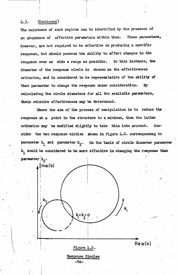
Figure 4.2.

Response Circles -54-

14.3. (Continued)

The existence of such regions can be identified by the presence of

an abundance of effective parameters within them. These parameters,

however, are not required to be effective in producing a specific

response, but should possess the ability to affect changes in the

response over as wide a range as possible. In this instance, the

diameter of the response circle is chosen as the effectiveness

criterion, and is considered to be representative of the ability of

that parameter to change the response under consideration. By

calculating the circle diameters for all the available parameters,

their relative effectiveness may be determined.

Where the aim of the process of manipulation is to reduce the

response at a point in the structure to a mtxbuun, than the latter

criterion may be modified slightly to take this into account. Con-

sider the two response circles shown in Figure 4.2. correspondong to

parameter k, and parameter Ic 2 . On the basis of circle diameter parameter

II Ic1 would be considered to be mare effective in changing the response than

.parameterjrc2 .

11m

4.3. (Continued)

However, where it is required to minimise the response parameter Ic,1

is ineffective, while Ic 2 is by comparison far more effective. Thus,

with the bias towards ninjinisation, a new effectiveness criterion may

be defined as the portion of the response circle for which the response

may be reduced over its present value. The amount by which the

response may be reduced can be represented by the line AD shown in

Figure it.). This, however, does not take into account the size of

the circle, and hence a more representative measure would be the length

of the are CD. Thiais referred toas the bias di00f the

circle.

The criteria that have been developed in this section have be

formulated in order to highlight certain qualities of structural

parameters. The best criteria for achieving desired response character-

istics can only emerge as a result at the experience gained in, using them.

Rect(k) Figure

The Portion of the Circle Effective in Decreasing the Magnitude

of the Response

• -55-

14.14. The Practical Application of Effectiveness Criteria to

a Helicopter Fuselage.

This chapter. deals with the practical application of structural

manipulation and would not be complete without an example to illustrate

the use of the techniques developed. In addition, the example

helps to define and explain more clearly the bases upon which the

effectiveness criteria lie. 4.

The example chosen is representative of the practical problem

which provided the incentive for this research. Under consideration

is the very much simplified two-dimensional model of a helicopter

fuselage. The structure contains 20 nodes Interconnected by 25

linearly tapering beam elements. Each node possesses three degrees

of freedom, two translation and one rotation, making a total, of 60

degrees of freedom. The layout of the model along with the element

and node numbering is shown in Figures 14.14. and 14.5. respectively.

Mass and stiffness data for the model was obtained from Westland

Helicopters Limited, whilst damping was included in the form of a percent-

age of critical damping in each normaJ, mode. The analysis was

performed using the structural maipulation programme described. in

Chapter 5, the aim being to deternlne which parts of the fuselage -

structure *ere most sensitive in reducing the rotor induced vi%ation

levels In the region of the pilot!'s seat (Node-18 in Figure 14.5.) The

* structure was excited by a sinusoidal torque, of frequency 21.7 Hz at

node :8. Both the vertical and horizontal responses at node 18 were

• examined, 4though only the results for the latter have been included

here. Only stiffness parameters connected between adjacent nodes were

considered. In this way parameter changes could be directly related to

existing struottwal elements. By Imposing this restriction the

'.

-56-

p

I-

Ig 5

• 15

, I.!

• I 12 13 -I •-

( I 17 ill

19 21 -12

14F 20

"a-

-%r 3 0 SPRING

Helicopter 'Stick Model' Element Numbering.

- I

St

9

03

/1 CD

/ g

/

Ji

( 2 -3D SPRING

Helicopter 'Stick Model' Node Numbering.

14.14. (Continued)

total number of parameters being associated with each element was

three • These are, defined in Figure 14.6 • The totsl number of

stiffness parameters associated with the structure was 75.

1 element

4

Parameter coordinates [1,41 [2,51 [3,61

Figure 14.6.

Stiffness Parameters Associated with an Element

Four criteria were used in order to determine those parts of the

structure which were most effective in reducing the vibration levels.

Firstly, by considering just one parameter at a tine, the following were

calculated for each of the 75 parameters:-

I Circle diameter.

Bias Diameter. ,

Minimum Response.,

The values loorresponding to (i) and (ii) have been sorted In

descending order and are normalise4 such that they lie in the range

0-1. The jralue one is assigned 10 the most effective parameter, and

zero to tS least effective parameter. It should be remembered that

these oritei,ia are used to determine relative quantities and are not

indicative of absolute effectiveness. Where mln4mtnn response is

59

(Continued)

concerned the values encountered are usually spread over a wide range

making them unsuitable for normalisation in the manner just described.

Consequently, the logarithms of the inverse of the minimum responses

have been calculated, sorted and normalised in the range 0-1.

Each parameter has associated with it three sensitivity values;

these are used in two ways to produce an equivalent figure for the

elements of the structure. Every element has associated with it

three parameters, the first value assigned to the element is that of

the most sensitive parameter. This is intended to show that if an

element has an effective parameter associated with it, then that element

is effective regardless of the effectiveness of the other two related

parameters. The second measure is the average sensitivity for the three

parameters.

The results are presented in the form of line graphs where the

ordinates refer to the various effectiveness criteria and the horizontal

axis represents the various elements of the structure • For each

element, the shaded ordinate refers to the best parameter value, whilst

the unshaded ordinate shows the average of the three parameter values.

The fouith criterion involves parameters combined in pairs. -

Each pair was assessed to see if it could produce zero response at

the pilot'4 seat. In the case of,. stiffliess, there were 75 parameters

and 2,775t possible paired conibinations, many of which satisfied the

required cflterion. The nwaber o tithes an element occurred in a

successful 'pair was noted and the results were tabulated in descending

order, having been normalised in the range 0-1 as before. This

measure . can be interpreted as providing the relative effectiveness of a

I -60-

14.14. (Continued)

given element to actually produce zero response in conjunction with

another undefined element. The results for element occurrence are

also presented as line graphs.

The four criteria outlined above were recalculated, only

this time the variable parameters were changes in point mass at each

of the nodes. The total number of parameters in this case was 60.

•

The results for variable mass are plotted as line graphs in exactly

the sane way as for the stiffness parameters. This time the numbers

• on the x axis refer to the structure nodes and have been arranged

in groups representing well defined areas of the structure. The

results for both variable mass and stiffness are given in Figures 14.7. -

14.14. It will be noted that in Figure 14.114. the ordinate referring •

to the best parameter value has been omitted. The values that

should have been presented here were an unity or very close to unity,

and their presence tended to obscure the remaining ordinates,

1

CD

b' I . (0

U) (1) C a) >

C) a) 9- 9-

w

/

___1—civercçje value .- best parameter per element

gearbox+ rutorhead gear box engine sides root floor tail boon floor supports fuselage -

Variable stiffness: Circle diameter.

1-cverage value -best parameter per element -

ii

0 U

Ia U)

tn U) 4) C a) >

-I-

U a)

I.- I.-

w

[01

gearbox .rotorhead gearbox engine sides root floor toil boom floor supports fuselage

Variable stiffness Minimum response

0 II L -, lI " 'ILi

gecr box. rotorheud gear box supports

engine sides roof floor tail boom

fuselage

1 -

ttoo r

Variable stiffness Element Occurrence [Zero response]

N

I0

ko in U) 0 C 'p > U 'p

w

average value I

—best parameter per element

- 1

CD

D r

C a, > 4-

U C)

'4- '4- w

n U

jI 2 3 4 5 it 6 7 116 9 10 11j112 13 141115 16j17j19 2021 22 231 1 24 25]

gearbox * rotorhect d gearbox engine si dé s roof floor tail boom floor supports fuselage

Variable stiffness Bias diameter

0

P.

1 IcS

I. Pt

S

.-average value • .best parameter per element

I

in in a) C

> .1

U a)

•4-

w

4- C

• I B 7 6 19 131112 11 20 1 1 5 4

gearbox rotorheud engine roof 2_ji 2 3 10 L14

floor.

nodes 15 15 17 118

tail boom floor

•Variable mass Circle diameter

/

• average value

best parameter per element

1

hi

1 CD

ro

• . 1 1 11. .

linodes 1 8 7 6 19 131112 11 20 jS 4 9 1 2 3 10 jilA 15 16 17 IllS i

gearbox rotorheud en gine roof floor tail boom floor

Variable muss Minimum response

E

1

0 18 7 6 19 13 1i12 11 20 1 5 4 9 112 3 10

- gearbox rotorheud engine root floor

N

'CD

czt. C) C C) >

4-

U 4)

I.-w

a) > ci C) ir

15 16 17

toil boom

1 1 nodes

floor

Variable moss Node Occurrence (Zero response]

average value 6ii

•(amitted

Ni

Ig 1W

Lb I•. U) in a) C 0) >

C, a)

'4-

w a) >

-4-. a a)

Er

0 8 7 6 19 13 1112 11 20 5 4

eurbax rotorhead engine roof

nodes 2 3 IO 1 14 15 16 17 11 18

floor tail boom floor

Variable mass B-ias chum

14.141. Discussion of Results.

It is already known that, for this particular helicopter,

• the gear box and tail boon are suitable areas for modification in

order to alleviate vibration in the area of the Pilot's seat. This

knowledge was gained over a period of time through a oeosa of triM].

• and error, helped by a limited anount of theoretical analysis. As a

result of this, the gear box mountings were considerably stiffened and

so was the tail boon between nodes 22 and 23.

The results for variable stiffness shown in Figures 4.7. -

1.10. are mutually consistent in that they show the same three sensitive

areas in the fuselage, namely, the gear box, tail boon and fuselage

sides • This agrees broadly with what is known about the helicopter.

What is interesting is that the same message canes across regardless of

the criterion chosen, which tends to indicate the relevancy of the

• chosen criteria. In considering these three main arec, the importance

of the gear box and fuselage sides is intuitively obvious. The former

since it is close to the source of excitation, and the latter because

of its ability to transmit forces, mainly in shear, to the front sub-

structure • The importance of the tail boom is not so intuitively

obvious an it is encouraging that the analysis has highlighted this area.

The results for variable mass shown in Figures 4.3.1. .

are reasonably consistent for all but the bias diameter criterion. The

gear box and fuselage sides are again highlighted as sensitive areas,

with nodes 6 and 19 being shown to be particularly effective by the circle

diameter criterion. The minimum response criterion shows nodes 8 and

18 to be sensitive in the reduction of vibration levels; this is

intuitively obvious since these nodes represent the forcing and examination

1.21. (Continued)

points respectively. An Infinite Increase in mass at either of these

points would effectively reduce the response to zero. It is

interesting to note how the sensitivity to changes in mass varies along

the tail born. The circle diameter, minimum response and node

occurrence criteria all indicate that relative effectiveness decreases

towards the end of the tail born. Where stiffness parameters are

concerned, with the possible exception of element 23, the circle

diameter and minimum response criteria indicate the reverse trend, i.e.

effectiveness increases along the tail boom. For both mass and stiff-

ness parameters the engine is indicated as a relatively insensitive area.

Of the four criteria used In the analysis of the helicopter

fuselage, only the bias diameter results have proved in any way in-

conclusive. For stiffness parameters the results are less well defined

but still indicate the same sensitive areas as the other criteria.

For mass parameters, however, the results sew to show no trends what-

soever; this seems strange when it is considered that the bias diameter

criterion contains elements of the circle diameter and minimum response

criteria, which both indicate clearly the sensitive areas in the structure.

The conclusions drawn here are tentative ones based on a -

limited aaltt?unt of experience in this particular field of interpretation.

The exercise was primarily intended to demonstrate the use of the

various crIteria developed In this section. However, although there is

still a wte'at deal of work to be done on the development of this

practical form of analysis, there is strong evidence to indicate-its

4.5. parameter changes in Bee]. Structures.

This section is complementary to the previous one In that it

deals with some aspects of the practical implementation of structural

manipulation. The emphasis here is placed on the relationship between

the simple parameters used throughout this analysis and those encountered

in real structures. The simplicity- of the aforementioned analysis cones

as a direct result of the form of the parameter changes chosen.

It would, however, be unrealistic to expect similar changes to be either en-

countered or useful In any practical. sense. What is required is a

direct relationship between the practical Structural parameters such as

beam dimension, web depth and skin thickness and the idealised linear

spring parameters. Progress can be made in this direction by

constructing an equivalent spring model of a simple finite element.

Consider the simple beam element shown in Figure li.lS(a). The

uniform bean, which is inextensible, possesses four degrees of freedom

r1, r2 , 1'3 and ru as shown, second moment of area I and Young!s Modulus

S. The stiffn sea matrix for the beam is well known and is given

in Figure 11.1(b).

By considering the equilibrium of the bean, the following

relationshij,s may be obtained -

F2 -F (U.n)

F3 I F1 - F4 F1 + F2Q.i (4.12)

Thepe two relationships hn]y an Interdependency between sane

of the elemnts of the stiffness matrix K. In fact, if elemeüts k ll p

Ic12 and Ic22 3 are known, then the values of all the other elements1 can be

determined using equation 4.3-1., 4.12. and symmetry. These t1ree texts

form the elements of the stiffness' matrix of the cantilever beam shown

-72-

-

\ri displacements

forces

2 (0)

A. 2 6 I PT

K=EI L •L L

SYMM

12

(b) stiffness matrix

p.4

12 A 41

equivalent spring.system

Beam Element and Equivalent Spring System

Figure 4.15. —73-

U.S. (Continued)

in Figure 14.16(a).

C

[A]

*j2 El 12

1

k+kx2 -kx

12 2

II

El

FBI Figure 14.16. -

Cantilever Beam and Equivalent Spring System

The equivalent spring system showi? in Figure 14.16(b) consists of two

rigid beams, total length t, hinted at a distance x from the free end.

A rotatiohal spring of stiffness It1 connects the beams at the hinge,

whilst a linear spring of stiffneès It2 is situated in the constraint

arrangement at the free end of the bean. For the two systems to be

equivalent, the elements of their respective stiffness matrices must be

the same. Hence, equating the relevant terms leads to the following

—74-

I.

14.5. (C6ntinu4)

values of 1c13 k2 and x

k1 1/L

Ic2 = l24

x - t/2

(14.13)

Using these values, the beam in Figure 14.35(a) may be represented

by the equivalent spring system shown in Figure 14.15(c).

The theory can be extended to cover the general case of a

linearly tapering beam with second moment of area 10 at one end

and a taper ratio r. The analysis proceeds along the same lines as

for the uniform beam, but requires that the stiffness matrix for a

Tapered beam be determined. This is given in Appendix K and refers

to a beam of I cross section. The stiffness matrix could, however,

have been calculated for a beam of any cross section. Equating the

elements of the two stiffness matrices as before gives the following values

of k1,k2 and x

kj-32 (2r2 +r+2)

SO

k21 (r4+4r3+lOr2+ ljr+l) (14.11)

U. (2r2 + r+2) -

x-Ø.(l7r2 +6r+7)

12 r2 + r

It will bet noted that These value's degenerate to those given in

equatipii 14013. when the taper ratio is unity.

It has been shown that a finite element beam can be modelled

in terms of the simple parameters used in the structural manipulation

theory.. These parameters are directly related to the real structural

variablr, E and I. However., the parameters Ic,1 and k2 cannot be

14.5. (Continued)

varied independently since they are directly related. This situation

leads to the consideration of a special case of parameter variation,

namely, two stiffness parameters varying simultaneously but in a.

related manlier.

Consider the simplest case where the two parameters kA and

have the following linear relationship.

Ic1 flk2 (14.15)

where/3 is a real constant. The response at a point in the structure

maybe given asa function of 'i and k2 and is

eaIe1 +bk +ck1k2 (14.16)

1 + dJc1 + ek2 +

where the constants a, b, c, d, e and £ are complex and are defined

In Appendix C. The constant G has been omitted from equation 1.16. for qp the sake of simplicity-. Substituting for Ic 2 from equation 14.15. gives

or k 2cfl+kja + bp) (14.17)

k12fp+k1 (d+ ep)+i

Equation 14.17. may be considered as providing a mapping from the

plane to the aplane. Any complex mapping such as this may be made up

of a series of simpler mappings. In this case, there are two mappings

which take the form H (4.18)

Ck,+D

and Ctl.Z2+E (14.19)

where the constants A, B, C, D and S are all complex. Equation 14.18.

is an example of a Bilinear Class of mapping and maps straight lines in the

1 —76-

144. (Continued)

Ic1 plane into circles in the z plane. Equation 14.19. maps the

circles in thez plane into Cassini Ovals in the c plane A

Cassini Oval or Cassinian is a higher plane curve of the sane type as

Cartesian Ovals, liinacons and carciloids (see Figure 14.17.). A

Cassinian is defined as the locus of a point which moves so that the

product of its distance from two fixed points ( 0, a) is a constant

Ic2 . The equation of this curve in cartesian coordinates is

(x +7 +0) - Isax -k

22 where c - Ic + a • If Ic < a, there are two separate ovals each

enclosing a focus and the curve is said to be bipartite. If Ic> a

the two ovals merge into one • When k a, the curve is a lemniscate.

The boundaries of the feasible response regions are examples of this

type of curve. Thus, when two stifibess parameters are varied in

a related manner, the response no longer lies within a feasible region

but ona closed curve whose form is determined by the nature of the

relations4p between the two parameters. The analysis of these curves

is known to be complex, but therej is sufficient justification for a

closer iniestigation into their mathematical properties.

A iiirect relationship bettieen real structural parainetei1s and

linear sprung elements has been sIawn to exist. The practical application

of the theLry developed around this work has not been attempted,,

but it is clear that real parameter changes can only be represented

by combinations of idealised parameters. The variation of these

parameters in a related manner imposes tighter restrictions on the --

response at a point in the structure than if they had been allowed to

vary inaePtndentty.

Curd ioid

Lemnicute

Limo

Examples of Special Cases of Cartesian Ovals

—78— Figure 14.17.

-N 4.6. Oher Techniques for Assimilating the Effectiveness of

Parameter Changes.

This last section contains some of the more interesting

aspects of the main analysis which have not been fully developed,

but which may have potential usefulness. A single response is

examined as a function of frequency and stiffness and the case of

multiple responses as functions of structural parameters is also

considered.

4.61. Response as a Function of Frequency and Stiffness.

In Chapter 3, an example was given of a three dimensional

response plot, for which the response was considered as a function of

frequency and stiffness. The plot consists of a set of response

circles representing a single variable parameter and calculated over

a range of frequency. If an infinite number of circles were plotted

In the given range, then a cylindrical envelope would be developed

upon which the response must lie for a given value of stiffness and

frequency, Figures !i.lS and 4.19. show two examples of these

plots, both were calculated using the mathematical model of the

experimental structure described in Chapter 6. These plots can be

used to givh sane indication of the effectiveness of single parameters

as a functin of frequency. The size of the response circle, which has

already been used as an effectiveijess criteria, can be plotted

against frequency and the resulting graph represents the relative

effeciveness of that parameter in a given frequency range. In order

to pr&iuce this graph, the frequency range of interest is chosen and the

circle diam4ter for the given parameter is calculated at a specified

number of points within that range. A curve is then fitted through

—79-

Rea(k) stiffness parameter' ,rdinqtes It )

Response as a Function of Stiffness and Frequency.

Figure

L —80-

Response as a Function of Frequency and Stiffness

jgure 4.19. -81-

15.61. (Cintinued)

these points and the resulting graph is shown in Figures 15.20. and

15.21. These are the circle diameter against frequency plots

referring to the same systems that were used to produce Figures 1.18.

and 4.19 they do, however, include the graphs for several other

parameters as well. The peaks in these plots may be interpreted as

being representative of frequency ranges in which the associated pan-

meters are potentially effective. The curves were produced using the

structural manipulation programme. The process by which they are

obtained can be time-consuming, for it involves calculating new

receptance matrices for each value of frequency.

15.62. Multiple Responses as a Function of Structural Parameters.

Consideration so far in this analysis has been given exclusively

to examining the behaviour of a single response as a function of one

or more structural parameters. However, it is often desirable to be

able to consider a set of responses collectively. In this section

a set of n responses are considered as a function of a single stiff-

ness parameter k. The sin being to calculate the value of k for which

the sum of ithe response vectors is a minimum. It will be shown that,

once form4ated, the problem cannot be tackled analytically but must -

be solved using an iterative procedure. The case in which the

responses are considered as a function of more than one parameter is

not considered.

In its simplest form the problem involves calculating the minimum

of a single response as a function of one stiffness parameter. This

case was dealt with in Section I.21., and was found to have an analytical

solution.

Consider a set of n responses ai and a single variable stiffness

-82-

cx u-i

.uJ

cc '-I

0

Lu —J Li ry I-,

CD

4:..

9 (2,0)

/ Parameter Coordinates.

(2,6)

(3,4 (i,a

(4,5)

331.4 1 I 200.0

FREQUENCY C/S Circle Diameter Against Frequency For Fi ve Parameters.

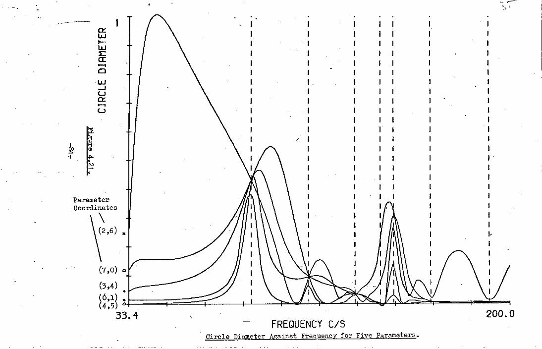
1 cit LU

Lu a

1

0

uJ —J 0 at C-)

IL a I\)

-- - a

Parameter Coordinates

\ (2,6)

(7,0)

(3,4) (ó,ì (4,5

33114

200.0 FREQUENCY C/S

- Circle Diameter Against Frequency for Five Parameters.

4.62. (Continued)

parameter k; it is required to find the value of k for which 1

is a minimum. If p is the point of excitation and the parameter Ic

isattached to the structure at points r and a s the response CC is

giyen by

- + k((G5 - G,)(G - G15 )) (4.20)ir

i+k(G +G -G -G ) rr as ra or

which may be written more generally

OCj u+ivi_ei+ffj+k(ai+ibi) (4.21)

1 + k(c1+id1 )

K

The real and imaginary components of are

ui - ei k(a + k(a1c1 + bd1 ))

1 + 2ck + k2 (o12+d12 )

and

vi fi + k(bi + k(bicj - aidj))

1+201k+k2 (c12 td12 )

Nbw 2 I

ku - u1 +

2 a - (L1k +B1kC1) 2

(P11c2 +Q1k + B1 )1 where A' i' ?i' P,$ S and R i j are defined in Appendix I.

The minisnin of the function 1&,Iis given when • n ni

d r kijE t 4_ lot li - o • 1 £-1 1 dk.

-85-

(4.22)

(4.23)

(4.24)

1.62. (Continued)

The first derivation of IC(.I with respect to k is

+ B1k + af1 (k + Bi)_(2Pik + Qj)(aik2+Bik + a1 )4

21

dk 2(P1k2 + Qlc + a1 ) 2 2(P1k2 + Q?+ 3/2

(1.25)

It will be noted from equation 4.20. that ?, Q1 and R are functions

of the position of the parameter it aily and therefore are the same

for an i. Thus

- (Pk cit + R1) -) - 2

((sit2 + Eic + aø (2A13c + B1 ))

dk 2

I- (2Pik + Qi)(Pit2 + + a1)"2 + B?+ C1 )4

2 (11.26)

Equating equation 14.26. to zero gives

"I (A 1yc2 + B1k+C1)2 3.

(2P1k +

451 (2A11c + B1 )(A1k2+B1k +

(14.27)

• which cannot be readily solved analytically. Consequently, the

root of equation 14.26. corresponding to the minimum value of k ij is obtained using an iterative search procedure. (Nottingham

Algorithms; Group Library Subroutine EOGBAF 1131 ), The routine

• requires tSe gradient of the function and a good initial estimate of

the required root. The latter is obtained by calculating the n

• mininwn oftS function which is assumed to be a good

approxtma4on of the required minimum and can be determined analytically.The (

sum t the squares of the moduli ,-vE the response vectors is given by

• Lt 1 2. (r1it2 + y+ n111 I (A/ + B1k + a1) (4.23)

N 4.62. (Qontinued)

If the first derivative, with respect to It, of equation 4.28. is

calculated and equated to zero then the following quadratic in It

is obtained

i2 (AQ1 - gp1 ) + 2k(ZR1 - q1 ) t - - 0 (4.29)

where

X= f-1 Ai

fl 1L- B1

.= In1 C1

Equation 14.29. can be solved and the root corresponding to the minimum

veins of 110C 1 1 2 is found in the usual way. from the second derivative

of The function. In practice the iterative procedure converges

rapidly using this initial estimate.

Using the structural manipulation progranne, the minimum of the

sum of a set of response vectors is calculated for all the available

stiffness xfiarameters in a given system. The results are sorted in

• ascending drder of minimum response and tabulated to give the sum of

the response vectors and the corresponding value of the stiffness

-87-

CEAnERS

COMPUTATIONAL ANALYSIS

5.1. Introduction.

The mathematical analysis outlined in the previous chapters

includes a certain anoint of matrix algebra, in particular the solution

of sigenvalue problems and the inversion of matrices. Where the order

of the matrices involved is greater than three, then the solution of

these problems becomes too complex to be performed by hand and it is

necessary to resort to the computer to perform these tasks. Initially,

programmes were written to perform specific operations in order to test

the theory being developed; however, it became increasingly obvious that

the canputer was going to become an indispensable tool playing a major

role in the development of the analysis. The programmes that had

already been developed were being expanded to provide ever more

detailed and diversified forms of information, and it soon becane

apparent that the process as a whole was becoming too slow and cauplicated

to be able to produce the required results in an efficient manner. What

was needed was a more general interactive programme capable of fast data

handling and with the facilities to perform any or all of the calculations

previously handled by separate pziogrammes. A Structural Manipulation

Programme was consequently written to rim on-line on the ICL 47

computer operated by the Edinburgh Regional Computing Centre. The

programme was intended as a research tool which could be expanded without

impairing !its performance and width could be run as a truly interactive

process by either speeding up or eliminating the time-consuming procedures

normally associated with matrix operations.

5.1. (bontinued)

In the sections that follow, it is not intended to give

a detailed description of the internal operation of the progranne,

instead the underlying concepts behind the programing techniques

and the general capabilities of the programme are discussed.

5.2 • The Structural. Manipulation Programme.

5.21. General Description.

The Structural Manipulation Programme, which contains

approximately 5,000 statements, is designed to run on-line using the

Edinburgh Multi-Access System. The input and output of data to and

from the process is achieved using a teletype, although there is the

capability of using other devices. The programme consists of a main

driver section and a set of 27 external routines. The driver section

contains procedures which allow the external routines to be selected

order to perform specific mathematical operations. The external

routines are designed as self-contained units which are independent

of the rest of the process in a manner which allows them to be added

to or deleted from the system without affecting the existing procedures.

Although the programme is large, the sections of it that are .ised in any

one given operation are by compar4son relatively small and can be

executed 'with the maximum of speed and efficiency. Thus, by virtue'. of

the way i4 which the programme is put together, it is integrated yet capabe of continuous development and expansion without impairing

the efficiency of the existing sections.

- T48 Structural Manipulation Programme is designed to perform

analyses on the mathematical modeits of real. structures. This usually

takes the form of mathematical op' pratiais which use data from the

receptance matrices of the relevant systems. The calculation of these

H V

5.21. (continued)

matrices is time consuming, but they need only be calculated once for

a given value of frequency. In very broth terms the programme performs

operations in three main areas, namely, reading in system data, calculating

the receptance matrices for the system and performing mathematical analyses ,

using the receptance data. The system data takes the form of mass

stiffliess and damping matrices, M. IC and C respectively. Where damping

is not given explicitly in the form of a matrix, then it may be

included as a percentage of critical damping in each normal mode. This

involves the calculation of eigenvalues of the system and also the

generalised transformation matrix formed from the associated elgenvectors.

The damping matrix in the generalised coordinate system can be

calculated from these values and then transformed back into the original

coordinate system, (details of this along with the calculatiofl of the real.

• and imaginary parts of the receptance matrix are given in Section 5.22).

A simplified flow diagram of the programme is given in Figure 5.1.

•

Once the system data has been read in and the receptwice matrices

calculated, then the main driver 1 section of the programme is entered

• and the jser is then asked to select any one of the 44 options available

in the programme. Some of the more important options are described -

• below. I

(t) The real and imag.naryarts of the receptance

matrix are calculated for a constant value of

frequency, option (1) allows this value to be

- changed and the new receptance matrices

• 'calculated. H

• The natural, frequencies and normal mode shapes

of the system can be listed.

-90-;

start new

Inpu t data

Dumping matrix N given?

es

Calculate receptor-ice matrix Q

t n t e r main driver

sec tion

Teletype

• Store mapping file

Data file-

Punch cards

Calculate the generalised recepta nce matrix Q from damping coeffs + eigenvuLues.

Transform back to original coord' system

lectall

[OSe

ption

'(I______

Exit ?

_fYe s

I STOP

E x t e mat

Routines

I I

I I I I

PROGRAM FLOW DIAGRAM

Figure 5.1.

-91-

5.21. (cntinued)

(in) Both mass and stiffness parameters can be

considered in the programue; a stiffness -

parameter is defined as the change in stiffness

between two mutually compatible points in the

structure which are referred to as the spring

coordinates • A mass parameter is defined as the

change In mass at one of the structural nodes,

this point being referred to as the mass coordinate.

There are no restrictions imposed on the points

at which mass may be varied in the structure.

Where stiffness is concerned, then any of the

foflowing restrictions may be applied to the

parameters:-

No restrictions, i.e. stiffness may be

varied between any two spring coordinates.

Parameters may be restricted to being

associated with existing structural elements.

Grounded parameters, i.e. a spring connected

between any point in the structure and gro4,

may not be allowed.

Option (in) may be used to impose any of these restrictoGs

on the selected parameters.

(ly) Structural Manipulation theory may be used to

determine what th& response at a point in the

structure will be for a given value of a para-

meter. This parameter change may be incorporfled

I, into the system by Inserting the parameter vat into

5.21. (Continued)

(Continued)

the structure stiffness matrix. If the

parameter value is Ic and the spring coordinates

are r and s, then the following elements of the

stiffness matrix are modified:

k(r,r)—* k(r,r)+k

k(s,$) -9 k(s,$) + Ic

k(r,$) —t k(r,$) - Ic

Ic(s,r) —3 k(sr) -k

• Option (Iv) is used to insert both mass and stiffness

parameter values into their respective matrices.

• Checks are made to ensure that the matrices

remain positive definite.

It will be noted in option (Iv) that the predicted

response should be achieved where that particular

parameter value is inserted into the stiffness

• . matrix, and the new receptance matrices for the

system are calculated. Where the damping in the

system was originally specified in matrix font,

then the response is achieved. However, where

the damping is specified as a percentage of critical

damping in each normal mode, then a change in the

mass or stiffness data results in a change of damping

since the latter depends on the eigenvalues of the.

system. Option tv) may be used to ensure that the

generalised damping matrix remains constant when the

modified receptance matrices are calculated. See

5.21. (Continued)

(v). (Continued)

Section 5.22. (Damping)

(vi) For a given parameter, forcing point and response

examination point, the data concerning the response

circle produced by that parameter change can be

listed. The foflawing data is given:

The diameter and position of the centre of the

circle, the response coordinates of the points

at which the parameter is zero and infinity and the

value of the minimum response.

(VII) Given the restrictions imposed by option (In) there

are procedures within the programme which will select

automatically all the possible parameter changes

within the structure. Option (VII) is used tb •

calculate the circle diameter, bias diameter and

minimum response for all the chosen parameters.

These three values are taken as being representative

of the relative effectiveness of the parameters. The

• I exact definition of these criteria is given in Chapter

Li, Section 14.3. The effectiveness criteria are

sorted, normalised in the range 0-1 and listed in

descending order. Where an the parameters are

• associated with elements , then a further analysis

is performed giving the relative effectiveness

structural elements based on the effectiveness of

the parameters associated with them.

-94-

0 •

5.21. (Continued)

(viii) Option (viii) uses the sane list of parameters

as is given in option (vii), on]y this time the

parameters are combined in pairs and each pair

is assessed to see it it can produce zero response.

The totsl number of parameters, the number of

possible paired combinations and the number of

pairs achieving zero response are listed. An

• element analysis smiler to that in option (vu)

is performed where the number of times a given

element occurs in a successful pair of parameters

• is tabulated in descending order, the values having

been normalised in the range 0-1 (See Chapter U,

Section 40.). When a given pair is successful

in achieving zero response, then the values of those

parameters can also be listed.

• (IX) The Structural Manipulation programme may be used

to plot out the following graphical infonnaticns-

Three-dimensional, response plots as

functions of frequency and stiffness.

-See Figure 4.18. and 4.19.

Graphs of circle diameter against frequency.

See Figure 4.20. and 4.21.

(a) The boundaries of the feasible response

regions. See Figure 3.6.

(d) The construction of feasible response

regions from response circles. See

Figure 3.4.

5.21. (Continued)

(x) Option (x) is used to consider a set of responses

as a function of a single variable stiffness parameter.

The sum of the magnitudes of the response vectors is

minimised as a function of the stiffness parameter.

The procedure may be used to select all the possible

stiffness parameters as in option (VII) and to

calculate the minimum vector sum for each parameter.

The vector sums are listed in ascending order, with the

values of the parameters used to produce then.

(XI) The programme contains its own finite element

capabilities which can be used to generate structure

stiffness matrices. Option (n) allows any system

data associated with the elements and nodes of the

structure to be altered on an individual, basis without

having to resubmit all the other associated

data. This may take the form of changes to mass or

inertia data, Young's Modulus, second moment of area of

beam elements, the position of structure nodes and the

connectivity of elements. -

(xii) Thei'e are procedures for listing the foflowing system

data:- Receptance matrices; the constants inyólved

in both single and aouble parameter response equations

(see Appendices A aid B), all the system data sch as

mass, stiffness and damping matrices, node coordinates and

• element connectivity.

5.21. (continued)

(1t1 t) The programme possesses the ability to retain

various forms of useful system data from one rim

to the next. This eliminates the need to re-

calculate data each time the programme is run,

thus saving time; in addition, the maximum amount

of information on the system is always available.

The following list gives an indication of the type

of data retained:-

Mass, stiffness and damping matrices.

Eigenvalues, eigenvectors and trans-

formation matrices.

The receptance matrices (calculated

for the last specified value of frequency).

All element and node data.

A complete record of all the systems ever

used and a description of the graphical

output from the programme.

A record of any alterations that have

been madej to individual systems.

Most of the optima not mentioned here perform only

trivia], tasks whièh are not directly associated with

structural manipulation. An example of the output

from the programme for some of the aforementioned

options is given in Appendix 3.

-97-

5.22. Programming Techniques.

File Mapping.

The Last data handling capabilities of the Structural

Manipulation Programme are achieved using the file mapping facilities

available on the ICL hiS computer. Normally, a programme allocates

storage space for the arrays and variables that are declared within

it and before any analysis can take place data must be read in aid

assigned to the relevant variables. This procedure must take

plac every time the programme is run even if the input data is the

same on each occasion. When the arrays are large, then the time

taken to read in the data can be quite considerable, and this is not.

desirable in an essentially interactive process. However, if file

mapping techniques are used, then once the input data has been read in

there is no need to repeat this operation on subsequent occasions.

Pile mapping involves the mapping of programme variables on to

a file. (A file is an area of computer storage space which is

assigned to a specified user process). The allocation of storage

space for programme variables is arranged to coincide exactly with the

space assigned to a stare mapping file • Thus, once values have been

assigned to these variables, then the data is stored from run to run

on the store map file, and when the programme is re-rim the sane storage

space is allocated for the variables and they automatically have the same

values assigned to them as on the, previous run. If the values of the

variables are changed whilst runn ing the programme, then these changes

are automatically echoed in the store map file. The maximum size 0±'

array the programme is capable at handling in this manner is about 60 a 60. For a system of this size the amount of storage space the programme

)

5.22. (Continued)

needs is approximately 294 K bytes, which is far in excess of what would

normally be allowed using conventional techniques. The maximum use

of the store map file is made by storing useful programme generated

data such as naturel frequencies and normal mode shapes In the saw

manner. Thus, file 'napping techniques not only save valuable running

tine, but also allow for larger anoints of computer storage space to

be used than would normally be possible.

Coordinate Systems.

One of the more important features of any mathematical model

is the coordinate system in which it is defined. Afl the information

concerning the model is given at points whose positions are defined

in this coordinate system. The information that is of interest here

concerns the node and element numbering and the numbering of the

degrees of freedom of the model. Two systems are used in the

programme, the user system and the redundant system. The node and

element numbering of the structure is the same in both systems, and

is arbitrarily defined by the user. The two systems differ in the

numbering of the degrees of freedom of the structure. If the

structure possesses n active degrees of freedom, m nodes and the -

maximum number of degrees of freedom for any node is L, then the

number of redundant degrees of freedom is given by

(txm)-n

Only the active degrees of froedo!n are numbered in the user system

whereas the redundant system inclxdes the inactive ones as well. In

both systems the numbers are assigned such that they increase sequentially

with the node numbers, This is best illustrated by an example.

Consider the simple structure shown in Figure 5.2. It consists of

-99-

5.22. (Continued)

Coordinate Sy-stems (Continued).

three inextensible beans rigidly connected at nodes 2 and 3. The

maximum number of degrees of freedom at any node is two and the number

of redundant degrees of freedom is five.

® node number

2 degree of freedom numbS

Figure 5.2.

Degree of Freedom Numbering in a Simple Structure -

The numbering of the degrees of freedom in the two systems is given

in TableE 5.1. and 5.2.

5.22. (Continued)

Node x y (rot)

1 0 0

2 1 2

3 1 .3

'S 0 0

Table 5.1.

User System

Node x y (rot)

1 1 2

3 14

3 5 6

14 7 8

Table 5.2.

Redundant System

In the user system the rigid nodes are identified by zero's.

Degrees of freedom 1, 2, 7 and 8 In the redundant system are identified as

being rigidly constrained by including them in a redundant list,

degree of freedom 5 is also included in this' list since it is equivalent

to degree of freedom 3. The redundant system has two main advantages.

Firstly, it is not necessary to store the degree of freedom numbers in

arrays since they can be calculated directly for any given node and

coordinate direction using the formula

DOF number a a + (b-l)* c -

where a is the coordinate direction (in the example x a 1, and y (rot)

a 2), b is the node number and c is the maximum number of degrees of

freedom per node. The second advantage concerns the automatic

selection of. parameter coordinates. The simple piece of progiamme

code shown overleaf selects the cordinates in pairs

-101-

% CYCLE I 1 21 9 C

% CYCLE 3 = 1,1, NODE

% CYCLE K = 3 21 2 NODE

= i + (j-l)* a

3-1+ (K-])*c

%REPZLT

%EEPEAT

S REPEAT

where B and S are the selected coordinates, NODE is the number of nodes

in the structure and C is defined above. The coordinate pairs are

checked against the list of redundant coordinates, and any pair containing

a redundant degree of freedom is rejected. The successful pairs are trans-

formed to the user system where they are checked for element association

and also for mechanical coupling with the examination point. This

physical coupling is an obvious necessity ât1erwise the variation of that

particular parameter would be meaningless. The test for coupling

between two points, i and j, is if the element G the receptance matrix

is non-zero.

Damping and the Calculation of the Receptance Matrices.

In simple mass, spring, dashpot systems, damping is specified

directly in the form of a matrix; in reality, however, damping is

seldom encountered in this form. Where complex structures are modelled

using finite element techniques, j then damping may be included in the model

in the I oim of a percentage of cr 1itical damping in each normal mode. The

lflawlitude of the damping factors can either

* is the computer symbol for multiplication.

-102-

5.22. (Continued)

be estimated or measured expertnentafly. In order to introduce

damping into the system, the equations of motion are transformed into

generalised coordinates using the generalised transformation matrix It

which is obtained directly from the aigenvectors of the system. It

is known that the transformation matrix It will uncouple the undamped

equations of motion of an N degree of freedom system in the foll owing way.

If the equations of motion of the undamped system are given by

+jn Q

(5.1)

Then, substituting for A in equation 5.1. using the generalised trans-

formation

(5.2)

where are the generalised coordinates of thesystem; and we-

multiplying by itT (the transpose of matrix B) gives

flTMR +RTKR0 (5.3) In Which

RTMR_M*= I

and

where Mn. ¶d lt* are the generafled mass and stiffness matrices

respectively and ek is the (N x N) diagcnal matrix of eigenvaluss X.

Now, if the damped equations of motion of the system are to

be u$coupled by transfonning to generalised coordinates, then the

generalised damping matrix E* will be of the form

Idiag(21w.1 (SJt)

where 7 ± is the damping factor in the ith normal mode and is the natural freqncy of the system. The forced generalised equations

-103-

5.22. (Continued)

of motion of the system may be written

H*4+E3e4+jc*a p 0 XL/b (55) whereF* -

The stea4y state solution for the response is given by

sale wt

where

G*F* (5.6) and

(3* diag C - w2 ) + 217 .w.wJ-1 (5.7)

which is the generalized complex receptance matrix for the system.

Equation 5.7. may be 'written in the more general form

*= !A+i!r' where Aisthe (WxN) diagonal matrix 0f terms

the (N x if) diagonal matrix of terms (27p.w). If the real and

imaginary components of 0* are 0* and fl* respectively, then from

equation 5.8. II

f+iej [A+iB]i (5.9)

Equating the real and imaginary parts of equation 5.9. gives

0* A - The 3 a (Sa;o) 1 1 :11

(5.11)

Equations 5.10. and 5.11. may be solved simultaneou sly to give 0* and • as functions of LandBasfouoys

and

-104-

5.22. (Continued)

Matrix A is chosen for inversion since the inversion of matrix B

which contains small terms associated with the damping of the system

might lead to numerical errors. The real and imaginary parts of

the generalised complex receptance matrix (1* may thus be calculated

from the eigenvalues of the system and the damping factors in each

normal mode. Equation 5.6. may now be transformed back to the

original coordinate system to give the response vector x as follows

x- GFaRO*.RTF

If the real and iaaginary parts of G are £ and 1) respectively, then

they maybe given in terms of The real and imaginary parts of 0* as

foflows

C - It Cit ItT

$ D - RThtRT

It is the elements of matrices C and D that are used in Appendix A

to calculate the constants involved in the equation for the receptance

as a function of variable stiffness.

If the damping matrix E had been specified explicitly then

the matrices A and B would have been calculated as follows -.

H all-lieu] H and

BECJ

The real and imaginary components of the receptance matrix C are now

given by -1

£ - [A+B 1 B]

and

a--nc 3-

- I -105-:

5.22. (continued)

It will be noted that the inversion of matrices when working In

generalised coordinates is simple, since the matrices involved are

all diagonal. Also with reference to Section 5.21. Option Cv), it

is matrix B a Z*Wi4iich is held constant in order that the damping

of the system remains unchanged when the eigenvaluss of the same

system are altered.

5.3. Conclusions.

A. brief description of some of the capabilities of the

Structural Manipulation Programme has been given. The pro granrw

which has been developed and improved over a two and a half year

period is at present in a well tried and tested state. It has been

shown to be a useful tool in the practical application of structural

manipulation and its development is not limited just to consideration

of ways of achieving minimum response at specified points In a structure.

Research is at present being carried out into the possibility of

adting the Structural Manipulation theory, developed here to tackle

the problem of flutter in aircraft lifting surfaces.. The aim would

be to manipulate the relevant substructure variables In order to

achieve a specified normal mode configuration. There should be

relatively, little difficulty In adapting the programme to produce results

relating to the effectiveness of parameters in changing a normal mode

shape.

• - Under normal operating conditions when the progranme is being

run a restriction of two minutes CPU* time is imposed, and

• L* Central Processor Unit.]

—106-

5.3. (Continued)

this tends to limit the size of systems that can be considered, and

also the scale of mathematical operations that can be performed. In

order to save time, wherever possible iterative procedures are avoided and

matrix analyses are performed using diagonal matrices. A great 4eal of

emphasis has also been placed on the production of concise results

which present Information in a qualitative rather than quantitative

form. The programme is intended to give a rapid analysis of a

simple structural model with the broad aim of producing results

which will Indicate, in the most general sense, those areas of that

structure which are most suitable for modification for the purpose of

reducing vibration levels.

ii

II

CHAPTER 6

EXPERIMENTAL ANALYSIS

6.1

Introduction.

The aim of the experimental analysis was to examine the dynamic

II

response at a point in a structure and to verify that the locus of

that response vector traces out a circle when the stiffness of a simple

spring element in the structure is varied. It was not considered

necessary to examine the more complicated situations involving two or

more parameters, for it was evident that the results pertaining to

these cases could be arrived at equally well by allowing each parameter

to vary individually in turn. Thus, if the form of the response

can be verified for a single variable parameter, then those results

involving more than one parameter may also be assumed to be true.

This is by virtue of the fact that the response circle forms the

constituent part in higher order cases.

As well as verifying the form of the response, the accuracy

of the values is compared with those obtained theoretically. The

latter must obviously depend very much on the degree of accuracy to

which the experimental structure can be modejued mathematically. In

order to determine the accuracy, the natural frequencies of the

experimental structure were measured and used as the basis for comparison

between experiment and theory.

To achieve the objectives, outlined above, a test structure was

built and a continuously variable stiffness element was designed to

opezate in conjunction with this.- The structure was to be realistic,

yet not unduly complicated by too many unnecessary degrees of freedom,

6.1. (Continued)

and consideration was to be given in its design to the ease with which

it could be modelled mathematically. A programme controlled transfer

function analyser was used to measure the response of the structure.

The experiment was divided into two stages; the measurement of

structural response as a function of variable stiffness, and the

determination of the natural frequencies, node shapes and damping

of the structure. The remaining sections in this chapter describe

the construction of the experimental equipment, the techniques involved

in the analysis and the measurement of the results.

6.2. The Design and Development of a Variable StiffnessElement.

6.21. General Specification.

Ideally, the variable stiffness element should have linear

characteristics and be continuously variable in a manner causing the

least possible disturbance to the experimental system. In the

preliminary design stages, four ideas were considered; an electro-

mechanical spring, interchangeable spring elements, an air spring and

a variable length cantilever spring. The first two ideas were rejected

on the grounds that they were unsuitable • Two prototypes of the air

spring were built, but the idea ws abandoned owing to technical.

difficulties. Finally, a variable length cantilever spring was designed

and incorporated in the structure.. This had the desired characteristics

and was used successfully to vary stiffness within the structure. A

briOf desriptia of each of the four ideas is given below,

6.22. The Electro-mechanical Spring.

Figure 6.1. shows the schematic representation of an electS-

mechanical spring, consisting of a solenoid mounted between two points

in a structure. A linear potentiometer is attached-between the same

-109_I

et er

6.22. (Continued)

two points and produces a signal which is directly proportional to

their relative displacements. This signal is used as the input to a

variable gain amplifier whose output is then fed directly to the solenoid.

The system is adjusted so that the solenoid applies zero toroe when the

structure is In equilibrium.

4

p

Figure 6.1.

Sãhexnatic Representation of an Electro-mechanical Spring

-110-

6.22. (Continued)

The stiffness of the solenoid can be varied, without

disturbing the structure, by altering the gain of the amplifier.

The inadequacies of this system are concerned with the solenoid.

Firstly, it is difficult to arrange for the solenoid to operate

efficiently in both the push and pull modes; and secondly, the

maximum force output and hence the maximum stiffness of solenoids of

a suitable size is not large enough to be compatible with the envisaged

stiffness of the experimental structure.

6.23. Interchangeable Spring Elements.

An adequate, though not altogether satisfactory method of

achieving variable stiffness in a structure is to use a set of

linear spring elements each with a different stffness constant.

However, the disadvantages of this arrangement include the limited

range of stiffness for a given spring size and the considerable

disturbance that would be caused in the structure when changing the

elements. This idea was only to be considered as a last resort.

6.24. The Air Spring.

The single acting air spring consisting of a column of air

trapped between a cylinder and a movable piston is used in a wide

variety of applications mainly connected with suspension systems. In-

most oases the highly non-linear nature of the air spring is either

used to some specific advantage or is considered to be of no great

importance., If the air spring is considered to be double acting as

shown in Figure 6.2., then for snail displacements the stiffness of the

spring may bs considered to be approximately constant,

-ill-

6.24. (Continued)

1..

Figure 6.2.

Double Acting Air Spring

By varying the initial pressure P0 in the cylinder, the

stiffness of the spring may be altered and a wide range of values

may be achieved without any undesirable increase in weight. I

Theoretically, the air spring offers reasonable scope for

development, and in the initial stages of the experimental investi-

gation a considerable amount of time aid effort was spent on its

design and construction. The project, however, never reached a

satisfactory conclusion and was abandoned. The design of the air -

spring is unfortunately marred by the technical difficulties

associated with its construction. These are severe enough to make

the time scale for the project qite unreasonable. The theory

of the air, spring and the state of progress achieved during its

development are discussed briefly here.

The system depicted in Figure 6.2. consists of a cylinder

of length 2 Q. and cross sectional area A.. A double shafted piston

is positioed centrally within the cylinder and held there in equilibrium

H

-112-

6.214. (Continued)

by equal pressures P 0 on either side. The gas within the cylinder:

may be considered to obey the adiabatic law.

1w1 constant (6.1)

where P is the pressure, V the volume and Tis the ratio of specific

heat for that particular gas. For the sake of simplicity, the latter

is considered to be miity in the remaining analysis. If the piston

is displaced from the equilibrium position by a distance x, then the

new pressures to the right and left of the piston are P1 and

respectively. From equation 6.1. these are related by

PV - P1V1 P1 L - x)A (6.2)

P0VP2V2 P2 (I+x)A

• The resultant force on the piston is then

(P1 - P)A - 2PALx : (6.3)

t2-ic2

If 12>> x then this may be approximated by

(P1-P2 )A - 2PAx (6.14)

t

which provides a linear relationship between force and displacement.

The discrepancy in using this approximation may be estimated from the '

graphs given in Appendix E which show the relationship between - and x for both equations 6.3. and 6.14. 2AP0

The en-or in the app' adnation can be seen to be small for values

Of up to: 0.3 where it is 11%.

Rating obtained a configuration with linear characteristics, it

is n required to examine the parameters affecting the stiffness of the

-113-

H

6.21. (Continued)

spring. The latter may be obtained from equation 6.14. and is given

rA k2PA

0 (6.5)

&

Once the physical dimensions of the spring have been decided upon,

varying the initial pressure p0 is the only means whereby the stiffness

of the spring can be altered. The length and area of the cylinder have

+

a definite effect on the spring's sensitivity to small displacements.

High sensitivities can be achieved using either large values of A or

small values of 2,. But as t- becomes small, it will tend to violate

the necessary condition that 93>> x2 far linearity in equation 6.3.

Considering a spring with a maximum working displacement of 0.25" and a

2.0" cylinder (1. - 1"), then the error in using the approximation in

equation 6.2. is less than 2%. Thus, although not critical, decreasing

the size of t, still further is not a desirable way of increasing the

sensitivity of the spring. However, increasing the piston area A t which

depends on the square of its diameter, is an effective way of increasing

sensitivity without introducing any undesirable characteristics.

The theory shows the air spring to be a viable concept; the

practical implementation of this however involves a considerable amount

of technical difficulty. The problems fall into two main categories.

The first of these involves the provision of dynamic, yet gas-tight

seals, whilst the second involves the minimisation of the friction forces

between moving parts. Two air springs were built in an effort to

provide satisfactory solutions to these problems. The experience

gained in each case provided useful information, but neither version

succeeded tin possessing the desired characteristics. Both versions of

-114-

6.214. (22ntinued)

the air spring are described here, and a discussion of the merits and

undesirable qualities of each is given.

Version I.

- The first version of the air spring is shown in Figure 6.3.

and consists of a closed cylinder containing a single shafted piston.

o rings inset on the shaft and the piston serve both as bearings and

as gas-tight seals. Both sides of the piston were pressurised throughj

the needle valves at either end of the cylinder. The gas used through-

out the initial stages of the investigation was compressed air being

generated from a portable compressor. The maximum available pressure

_was flØ; p.s.i.

The air spring was tested in the horizontal position using

an initial pressure of 50 p.s.i. and with a 2 lb. mass attached to

the piston.With the cylinder clamped, the piston was excited by an

electromagnetic vibrator over a range of frequencies. The system

exhibited no form of magnified response. Large friction forces were

found to exist between the 0 rings and cylinder, although these were

considerably reduced once the piston had been set in motion. The

unbalanced effect caused by having only one shaft on the piston was

sufficient enough to cause it to creep down the cylinder. It was

found that even when subjected to the maximum available pressure of

nO p • s .i ., the small displacement encountered ( .050") was in-

sufficient to cause any significant resultant force on the piston, i.e.

there was no effective spring action.

Version II..

In the light of the obseryations made from the first air

spring,. Version fl was desigied incorporating the following modifications;

- -115-

material? Steel

gas •Yo'rina nflr

I .I I 0 IL.J

8 .

At' Spring Version I

Version II (Continued)

A double shafted piston mounted in linear p

bearings to eliminate any radial loads on

the 0 rings.

The use of maximum tolerances to reduce

friction.

Increased piston area and reduced cylinder

length to increase sensitivity to s7nall

displacements.

A flexible diaphragm between the piston

and cylinder instead of an 0 ring.

Greater accuracy in the manufacture of all

parts.

The use of CO instead of air (maximum

pressure 750 P.M.).

Apart from incorporating several improvements to reduce friction,

Version II of the air spring was designed in order to achieve increased

seüsitivity and also to assess the effectiveness of using a diaphragm

as a flexible seal between the piston and cylinder rather than an 0

ring. It was hoped that whilst still retaining an effective gas-

tight seal this arrangement would allow sufficient freedom of movement

•

yet not possess any of the undesirable frictional qualities of its pre-

decessor. Figure 6.4.(a) shows the layout of the spring. The

• length of the cylinder has been reduced to one inch CL 0.5"), which

• with the maximum expected displacement of 0.1" causes the departure from

the linear law to be only US. Te4ts were carried out initially to determine the ideal material

-117-

1' Internal diameter 3 stroke'* - .5'

material. -- Aluminium

•:-ci ring gas inlet

d

gas in LW

2.75'

2'

(Q)

cylinder

iaphragm

distorted diaphragm

(b) (c)

Air Spring Version II

Figure 6.4. —118-

6.24. version II (Continued)

and optimum size for the diaphragm. Firstly, several thicknesses

of rubber sheet were tried, ranging from 0.015" (surgeons gloves) to

0.1" thick. In each case these proved to be too flexible and were

epfly 4efonne4 y the sugtant4al pressi!P ferSices 4thin the

cylinder (see Figure 6.4-W). Next, steel shim varying in thickness

from 0.002" to 0.01" was used in an attempt to obtain flexibility

yet eliminate any stretching of the diaphragm. Besides changing the

thickness of the steel, the ratio of the area of the diaphragm to that

of the piston was also varied (see Figure 6.4-M. However, when

sufficient latitude of movement had been achieved the diaphragm soon

cracked due to fatigue. Considerable difficulty was also experienced

in obtaining a gas-tight seal between the two halves of the cylinder.

This was most probably the cumulative effect of using a gasket rather

than an 0 ring to provide a seal, and the increased forces accompanying

the higher gas pressures. No frequency response characteristics were

obtained for Version fl.

6.25. The Variable Length Cantilever Sprin

Originally, it was intended that the variable stiffness element

should be capable of being attached between any two compatible points

in the structure. By restricting the generality of this statement and

considering only the simplest form of parameter variation, namely a

linear spring with one end attached to the structure and the other end

to ground, it is possible to construct the equivalent system shown in

Figur 6.5i }; This consists of a cantilever beam clamped at the lower

end and attached to the structure at the other via a rigid connecting

rod. Rotational releases at either end of the connecting rod ensure

that &dy iorizontal forces are transmitted to the structure. The

—119-

6.25. (Continued)

cantilever applies an external force to the structure which is

proportional to displacement and is given by

F3EIx (6.6)

13

where E is Young's modulus for the material and I and U. are the second

moment of area and length respectively. The stiffness at the end of

the cantilever can be varied by altering its length; this is achieved

using an adjustable clamp, details of which are given in Appendix F.

The arrangement is simple to operate and is capable of producing a wide

range of stiffnesses.

structure

cantilever

rotational - - releases

- adjustable clamp

I Figure 6.5(1)

-

Variable Length Cantilever

—120-

I I I.

6.3. The Test Structure.

The test structure which is made up of steel blocks inter-

connectemy spring steel strips is shown in Figure 6.5.(a). The

dimensions of the structure were initially determined in order that the

highest natural frequency of the system should not exceed 159 Hz

This restriction comes as a result of thO limited resolution of

frequency in the oscillator that is used to drive the exciters • For

frequencies up to 159 Hz , the resolution is 0.1 Hz, after which it

Increases to 1.0 Hz. The disadvantages of the latter are obvious.

Through a process of trial and error the 6" x 4 rectangular arrangement

shown in the figure was found to have natural frequencies in the range

0-159 Hz.

The test structure consists of eight 1.75" square steel

blocks Inter-connected by 1.0" x 0.063" spring steel strips to form

a 6" x 14" rectangular grid. The structure is considered to possess

ten degrees of freedom, two translations and eight rotations. For

reasons that will become apparent later, this was reduced to eight by

constraining degrees of freedom 9 and 10 (Block 8 rigid). This

arrangement increases the stiffness of the structure and causes the

two highest natural frequencies to exceed the desired limit of 159 Hz.

This undesirable characteristic was considered unavoidable at the time

the modification was made. The modified structure is the one referred

to throughout the rest of this section.

Tho blocks, each representing a structural node, consist of four

0.875" x 0.875" x 1.75" slotted sections and are joined together as

shown In the exploded diagram in Figure 6-5- M. The blocks are

• deliberatey made large in order that their mass should be very much

• greater than that of any attached instrumentation. A hole drilled

- { -121-

I number [a] Nscionrop nf frdnm

-r

[bi

Test Structure and Node Block

Figure 6.. —122—

6.3. (Continued)

centrally through the block allows for the attachment of accelerometers

to measure the horizontal and rotational acceleration at that point.

A representation of the latter is achieved by mounting an accelerometer

off the centre line of the block with its least sensitive axis in the

horizontal direction.

The structure is excited externally in either of two ways,

horizontally at block 1 or in the form of a torque at block 2. Both

these forms of excitation are necessary in order to properly excite the

normal modes of the structure. The horizontal excitation force is

transmitted to the structure via the coupling arrangement shown in Figure

6.6. 1 -

retaining springs

exciter structure

gauge

Figure 6.6.

Coupling Mechanism from the Exciter to the Structure

—123-

II

6.3. (Continued)

The coupling consists of two pointed spigots attached to the

vibrator and structure; a piece of 0.25" aluminium dowel completes

the connection and is located in position by dimples at either end.

The retaining springs are tensioned sufficiently to prevent the

connecting bar from falling out when the coupling is in tension. The

system only transmits horizontal forces to the structure and allows

for a certain degree of misalignment between the two spigots, thus

minimising any lateral forces on the exciter.

The application of a pure torque to the structure was originally

achieved using the arrangement shown in Figure 6.7.. (see also photo-

graph (8) in Figure 6.8.). The torque was generated at the fixed end

of the coupling by means of an offset vibrator as shown in the figure.

This was then transmitted to the structure via a torque tube and a set

of two expandable bellows • The bellows were included to allow any

horizontal motion of the structure relative to the exciter • This

system resulted in sane undesirable non-linear effects and was later

replaced by the rigid bar shown in photograph (Q in figure 6.8. In

practice the structure exhibits very little horizontal motion when

excited in the rotational mode and consequently the increased flexibility

introduced by the more rigid connection does not significantly affect -

the measurement of the higher nods of the system. The cantilever

spring described in Section 6.25. is attached to the structure at block

U, thereby allowing the stiffness to be varied in the horizontal direction

at that point. A general impression of the test structure may be

obtained from the photographs in Figure 6.8.

-124-

II

Aluminium bracket

Exciter

ci

Generation of a Torque

Figure 6.7. —125—

........ axis

rig springs

minium dowel

force

AL

1 T '4

P

i~~T -

a"

iL S

moo

n Bellows Couplings. Figure 6.8. —1

4

'OIjiV Using a Rigid Coupling.

'[-'/

E I

L~

lid

ID)

orL oral Exciter. Figure 6.8. -127_

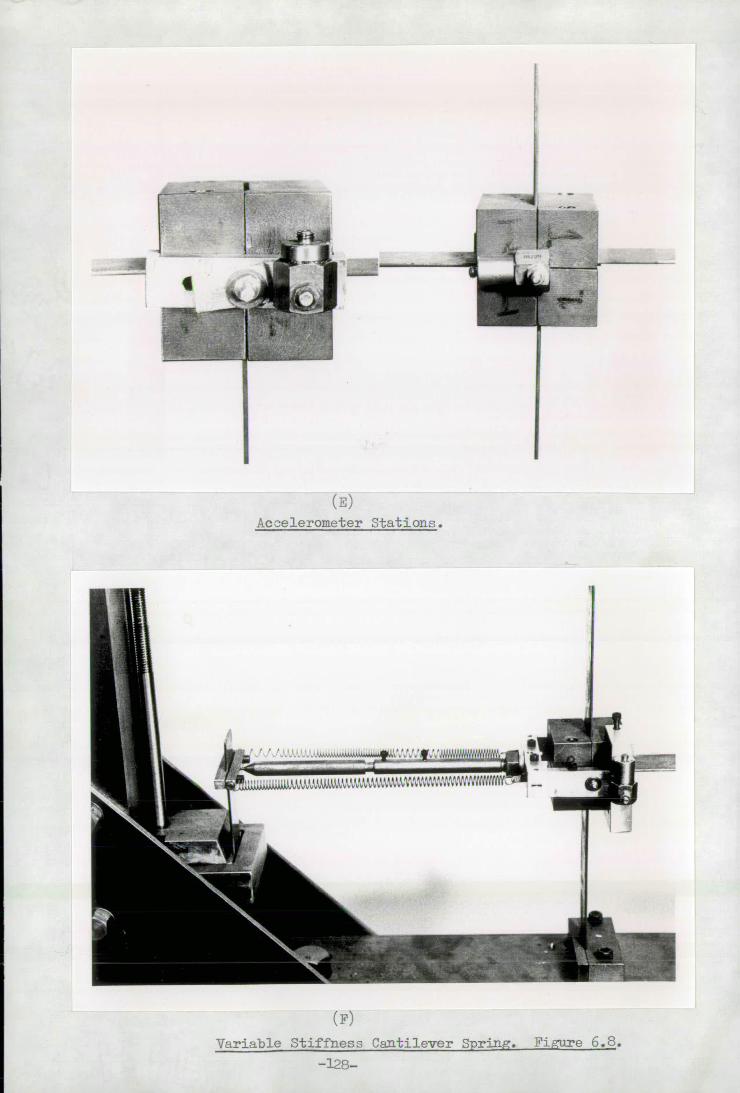
P

t I ~ 4~ k

±1:1

4 -

l-1IAL

C--

I

•1 t':

A

;.c :J c rometer Stations.

(F)

rjb10 tifness Cantilever Spring. Figure 6.8.

0

1<)

6.3. (Continued)

At the beginning of this section, it was mentioned that the

original test structure was modified in order to rigidly constrain

degrees of freedom 9 and 10 at block 8. This modification was made

after csep.g he réauls of an initial investigation into the

way in which structural response varies as a function of stiffness.

It became apparent that the response locus was not circular as had

been predicted, but appeared in the form shown in Figure 6.9.

Figure 6.9.

Response as a Function of Stiffness in the Origins]. Test 1 Structure

—129-

6.3. (Continued)

The locus shown here is characteristic of the one produced

when two stiffness parameters, one very much more effective than the

other, are varied simultaneously and in a related manner (see Chapter U,

Section U.k.). Thus, it would appear that the stiffness element

connected at block U was somehow affecting the stiffness at that point in

more than one direction • The most likely cause of this would seem to

be the non-symmetric nature of the structure at the point of attachment

of the variable stiffness element. By making node 8 rigid, the symmetry

of the structure was restored; that is with respect to block U. A more

-- - comprehensive explanation of this phenomena cannot be given, but the

fact that an almost perfect circular locus was obtained when the afore-

mentioned modifications had been included would tend to indicate that the

Previous assumptions were correct. The results presented in the latter

• part of this chapter refer to the modified structure.

6.4. &perimental. Equipment.

The experimental, equipment was intended for the purpose of

measuring the response at a point in a structure. Figure 6.10. shows

a block diagram of the system which consists of a Program Controlled

Transfer Function Analyser (PCTFA) with associated peripheral equipment,,

and the test structure itself. The PCTFA was used to control the -

experimental variables and to take response readings. The system

comprises a solartron .JN1600A Transfer Function Analyser (Tm), with a

high frequency extension wtLt, these being controlled through an

• interface ly PDP8 mini-canputer. The PCTFA provides the following

capabiljtiess\

Automatic frequency response measurement.

Multi-point analysis (up to 30 channels).

iii), Display of response readings on an Ir plotter or

-130-

y plotter scope

low speed Dun ch

teletype TRANSFER FUNCTION ANALYSER

remote control

N

power

signals from amplifier accelerometer

charge

amptiflers STRUCTURE vibrator

signai display scope

Schematic Representation of Experimental Fuipment

Figure 6.10. -

-131-

(Continued)

Cathode ray tube.

On line programme development and processing

of measured data.

The parameters under software control are*

i) The magnitude and frequency of the driving

sigma].. I

Input sensitivity.

The number of cycles of integration in the

correlation process.

iv) Input channel selection.

• v) An analogue output to plotter or scope.

vi) Provision for the additional input or

• output of information in the form of a

• Binazy Coded Decimal Number (BCD), providing

an alternative control channel to the tele-

type.

The software package incorporated in the system is a modified

• version of DEC FOCAL 8 called Dynamic FOCAL. This includes the

necessary commands for controlling the transfer function analyser.

Details of the operation may best be obtained by describing a

typical sequence of operations leading up to the taking of a response

reading. The frequency and magnitude (0-17) of the driver sigma]. are

set up using the oscillator contained within the Tfl. This sigmal is

then fed through a power amplifier to a vibrator which excites the -.

system under test. Signals from the accelerometers attached to the

I' structure are then fed back to the PCTFA. via suitable charge amplifiers.

On the presnt system cn2y ten of the thirty channels are operative. For

• • •• -132-

6.4. (Continued)

any chosen channel the input signal is connected to the digital correlator

whose input, sensitivity is set to "auto range" to find the right input

level automatically. At this stage the correlator picks out only the

fundamental sine wave component in the signal and rejects the noise

content and all Other harmonics. This is achieved by multiplying the

waveform by sine and cosine reference signa3s derived from the fimotical

generator. Digital integrators in both the sine and cosine channels

average their respective multiplier outputs for a period equal to a

finite number of cycles of the excitation frequency. The correlation

process has the effect of rejecting all harmonics other than the

fundamental. Noise rejection, however, increases with the number of

cycles of integration, which may be set to l( 100 or 1,000 cycles of the

fundamental frequency. The outputs from the sine and cosine integrators

are directly proportional to the "In phase" and "Quadrature"

components respectively of the waveform being measured. These may

be displayed as cartesian, polar or log polar coordinates.

The major proportion of the available 8K of storage space in

the PDP8 computer is taken up by Dynamic Focal, which leaves only

enough space to store 75 pairs of response coordinates. Although

somewhat restrictive, this is normally adequate for most purposes and

allows sufficient scope to perform simple mathematical operations,

such as sorting and scaling, on the stored data. The facility for

displaying the data on an oscilloscope allows instantaneous viewing

of experimental results, of which particular importance is attached to

frequency response plots.

The apparatus thus constitutes a fully integrated system

capable of. the automatic control and measurement of the dynamic respnse

6.4. (Continued)

of a structure. The photographs given in Figures 6.11. and 6.12.

give a general impression of the equipment.

6.5. Experimental Procedure.

The experimental procedure may be divided into two sections.

The first of these is concerned with the measurement of structural

response as a function of variable stiffness; the second refers to the

measurement of the natural frequencies and normal, mode shapes of the

structure. Both of these involve the measurement of response, the

former being at constant frequency, whilst the latter require that

a set of response readings be taken over a specified range of frequencies.

Each response reading has associated with it a phase angle which

is defined with respect to the reference signal generated by the TFA '5

interns], oscillator. It is common practice to take this same signal as

being representative of the sinusoids]l, force input to the structure from

the exciter, in reality, however, this signal is not a strictly true

representation. The force applied by the exciter is proportional

to the current passing through the coil (when stationary) and is also

dependent on the impedance of the structure to which it is attached.

In both cases considered above, the impedance of the structure does

change and thus the input voltage to the exciter cannot be taken as

• being truly representative of either the magnitude or the phase of the

force output.

The magnitude and phase of the force input to the structure can

be determined by means of a force gauge inserted between the exciter and

structure. The phase relationship between the response and the true

force input can be calculated from the separate phase angles between

each of these and the original reference signal. If the magnitude of

—134-

7 4

fah I

IVf KNM MOO

•L. - •.... •0ø••

r ...a

b

.JI t

The Test Structure and Associated Equi pment.

Figure 6.11.

lety-pe and U Plotter. Figure 6.12 .

- T-

6.5. (Continued)

the true force input changes then the size of the response vector

can be compensated for accordingly. Figure 6.13. shows the response

vector in both the true force coordinate system and in the coordinate

system referring to the reference signal.

ti

'I

- - - - - - _;esonse vector

F True forte

for e system

- id Re

Reference system

• Figt'e 6.13.

Force Reference Coordinate Systems

—136-

6.5. (Continued) I

If the magnitude of the forcing vector obtained on the first

reading in any given set is taken as a reference and all subsequent values

are adjusted accordingly, then the coordinates of the response vector in

the true force reference system may be calculated as follows. Let the

cartesian coordinates (in the reference system) of the force and

response vectors be (a,b) and (c,d) respectively, and the magnitude

of the forcing vector on the first reading be e • Then the coordinates

of the response vector in the true force reference system are (z: "y)

where

xe (ac +bd)

2 a 2 +b

and y - e(ad - be)

2 2 a +b

All subsequent readings can be adjusted in this manner, thus effectively

compensating for any changes in the magnitude and phase of the true

force input to the structure.

6.51. The Measurement of Structural Response as a Function of

Variable Stiffness.

The aim of the first part of the experimental analysis was

to be able to reproduce the circ4ar locus for varying stiffness

predicted in the theory. Ideally',, the point at which the response is

examined was chosen to be particularly sensitive to any variation in the

stiffness parameter. This sensitivity was maximised by choosing an

excitation frequency close to, but greater than, one of the natural

frequencies of the system, and by attaching the stiffness element at a

point in the structure which possessed a large amplitude of vibration

in the normal mode associated with this frequency. Also the stiffness

—137—

6.5. (Continued)

element was varied over a sufficiently wide range of values so as to

produce as large an arc of the response circle as p08 sible • The exact

frequency at which the experiment was carried out was determined by a

process of trial and error based at the quality of the results

obtained. Having chosen the values of the various experimental

parameters, control was passed to the PCTFA. Here, a small progranmte

was written to control the experiment and required as initial input

data, the magnitude and frequency of the excitation signal and the

number of cycles of integration to be used in the correlation process.

The computer was now set up to take response readings and store them.

The measuring cycle was started by remote control using the external

input facility of the POTFA. This eliminated the need to use the

teletype as an input device and also meant that the entire experimental

analysis could be performed in the proximity of the test structure, the

latter being situated some distance away from the POTFA.

A typical measuring cycle involved the following steps z II

i)

The variable stiffness element was set to

maximum stiffness.

The programme was started and the necessary

• parameters read In.

The structure was excited at the required

magnitude and frequency and allowed to settle.

The measuring cycle was initiated by remote

control and a respcçse reading taken. •

v) The stiffness of the variable element was

• reduced by a small Smount and another reading taken.

—i3

6.51. (Continued)

Altering the stiffness of the cantilever entailed loosening

a retaining bolt and lowering the clamp by means of the screw thread

arrangement shown in Appendix F. The clamp was uniformly tightened

after each change using a torque wrench. The measuring process was

repeated until sufficient data had been collected, at which time the

sequence was terminated. The response readings were sorted, scaled

and displayed on the screen of a storage oscilloscope. The information

was presented as a series of points in the complex plane. If the data

was satisfactory, then a hard copy was obtained on an XI plotter and

in addition the coordinates of each point were punched out on paper tape.

The following information was also noted:

The magnitude (lb f) and frequency (Hz) of the

excitation force.

The calibrated output of the accelerometer (V/g).

Any scaling factors involved in the measured data.

The examination and forcing points and the

position of the stiffness element.

6.52. The Measurement of Natural Frequencies, Normal Mode Shapes

and Associated Damping.

Although not the most important part of the experimental

programme, the measurement of natural frequencies and normal mode shapes

is ncessary since they form the basis for comparison between the

experimental and theoretical models • The results are obtained using

simple techniques rather than some of the more comprehensive methods

developed in the recent past [io, fl, 12] The time taken to develop

working versions of these techniques is disproportionate with their

desirthuitY within this analysis.

—139-

II

6.52. (Continued)

The method initially involves identifying the nature], frequencies

of the structure from a frequency sweep performed by - hand. The

response signal from the accelerometer under consideration is dispived

on the y axis of an oscilloscope in conjunction with the signal

representing the force input on the x axis. The resulting trace is

a lissajoux figure. This nthoi of examining the response shows the

change in phase as well as magnitude when passing through a natural

frequency, and hence is a more satisfactory method of identification

than the peak amplitude method. Also noted at this stage is the degree

of freedom with the largest amplitude of vibration at each natural

frequency.

These initial estimates are now used as the basis for an

accurate frequency sweep in the neighbourhood of the natural frequencies.

This time, the POTFA is programmed to vary the frequency, select the

input channel and take the response readings. The resulting vector

response bci are then analysed to produce \a revised calculation of the

natural, frequencies; this being based on the point at which maaum

spacing occurs between successive response points taken at equal inter-

vals of frequency. Figure 6.14. shows a typical vector response plt.

-

6.52. (Continued)

0C (0j)

-

6 -

(w)

Figure 6.14.

Typical Response Locus

A circle is fitted to the experimental data in the region of the

nature], frequency. If F is the nature], frequency and F1 and F2

are frequezcies at points 900 displaced to each side of this, then

from a graphical analysis of the vector plot the damping constant 7 for that particular mode can be calculated using the equation I

2]

- F

If the circle does not coincide with the experimental, data for as much

as 1800, thbn the damping may be calculated using the alternative

expression

—141—.

6.52. (th,ntinued)

f 2(I?3 - Fu) (tan i - tanc2)Fn 2 2

where F3 , F1111 and(X 2 are as defined in Figure 6.14.

TO measure the normal modes of the structure, the system is

excited at each of the natural frequencies in turn. An initial estimate

is obtained from the magnitude of the response signals from each

accelerometer. An attempt is made to identify nodes in the normal

mode using a stroboscope to highlight the movement of the structure.

-. - Besides this visual approach, the structure is examined physically

by touch to sense the vibration. This additional information proves

useful when analysing the experimentally calculated normal mode vectors.

Alter this preliminary examination, the POTFA is programmed to excite

the structure at the required frequencies and to obtain the response

readings for each of the eight degrees of freedom making up the normal

mode. The accelerometers attached to the structure have lMividnal

variable gain amplifiers and prior to taking normal mode readings:

the amplifiers are adjusted such that they all give the same magnitude

of signal when their respective accelerometers are being subjected to lg

acceleration. This matching of the accelerometers is necessary for the

normal mode data to be meaningful. Having obtained a set of response

readings for each normal mode, the data is analysed to give the

magnitude Of each vector and also its real and imaginary components in the

complex plane. The magnitudes of the vectors in each node are sorted

and normalijed such that the highest value is unity.

The! method outlined in this section may be relied upon to give'

reasonably accurate estimates of the natural frequencies of the structure.

• .1 H

1 —142-

6.52. (Continued)

However, those frequency response plots obtained in the frequency

range above 159 Hz do not possess a sufficient degree of resolution

to allow any meaningful graphical analysis. The natural frequencies

in this range are obtained using the peak amplitude method, whilst

the corresponding damping coefficients are estimated by interpolating

data from the sparsely populated vector response plots.

The experimental techniques used to produce the norms], mode

vectors of the system includes certain approximations which may provide

grounds for casting doubt upon the accuracy of the results. The

first approximation involves the instrumentation used in the measure-.

ment of rotational response. Figure 6.15. shows the position in which

the accelerometer is mounted in order to pick up the rotational

response of the block.

-. -Ox

accelerometer -

I

Figure 6.15.

The Measurement of Rotational, Response

-143-

A

6.52. (Continued)

Any given rotation ft of the block results in a displacement

in the zz direction which coincides with the most sensitive axis

of the accelerometer. However, any coincident motion in the n

direction will also be picked up by the accelerometer and will tend

to distort the originally desired signal. It is fortunate that

the accelerometer is only 10% as sensitive in the n direction as

it is in thezz plane, which helps minimise the effect of this un-

wanted signal. The second, and probably the most important factor

influencing the normal, modes concerns the degree to which it is

possible to excite a pure normal mode. In theory, the structure

should be excited at at least as many points as there are degrees

of freedom in order to produce a pure norma]. mode (undsnped). In

practice it is usually possible to excite a reasonably pure mode using

only one vibrator; however, the exciter must be positioned favourably

within the structure to achieve the maximum effect. In the investi-

gation under consideration the exciters were positioned on the basis

of the theoretically produced modes and remained in the chosen

Position throughout the analysis.

Thup, the experimental normal mode data may firstly be

distorted * unwanted signals aid, secondly, it mq not be represents-tin of the 1 pure normal modes of the structure.

fl ..

-144-

II

6.6. The Mathematics]. Model of the Teat Structure.

The importance of a mathematical model as a link between

experiment and theory should not be understated. Moreover, just

as the accuracy with which experimental results can be obtained sheds

light on their validity, so does the relevance and accuracy of the

mathematical model. However, before experimental or theoretical

data can be used in confidence for the purpose of comparison, there

must be reasonable justification for thinking that the mathematical

model is a good representation of the real physical system. This

essentially involves laying down a set of criteria for comparison,

in this instance the natural frequencies of the two systems have been

chosen. Since the experimental results are considered to be fixed

than the mathematical model must be manipulated to achieve the best

possible fit with reality. This in itself is a difficult under-

taking.

The mathematical, model shown schematically in Figure 6.16.

consists of 12 nodes, five of which are considered to be rigidly

constrained. The nodes are interconnected by 14 plane bending

elements which are considered to be inextensible. With the maximum

number of egrees of freedom being two, there are 16 redundants leaving

B active degrees of freedom. The numbering of the elements, nodes and

degrees at freedom is also shown in Figure 6.16. The mass and

inertia of the system are considered concentrated at the nodes,

whilst the stiffness matrix is assembled using finite element

tecthiques. In the first instance, the mass, inertia and stiffness

data are taken as the measured values from the test structure.

Damping is included in the model as a percentage of critical

damping ineach normal mods. I

-145-

• 6.6. (Continued)

One major difference between the mathematical model and the

teat structure concerns the modelling of the structural nodes. In

practice, these have finite dimensions and the stiffness elements are

not connected at a point. The element stiffness matrices used in

the mathematical model provide a relationship between the forces and

displacements at the ends of each element. But on the test structure

the equivalent parameters are measured at the centre of each block

which is rigidly connected to but displaced from the end of the

•

bean. In accordance with this, the element stiffness matrices may

be transformed into a new coordinate system which coincides with the

centres of adjacent blocks. Details of this transformation are

given in Appendix H. The presence of the variable stiffness element

was accounted for in the mathematical model by adding the appropriate

• stiffness value directly into the stiffness matrix (see Appendix J).

The natural frequencies and normal mode shapes of the structure

were calculated and compared with those found experimentally. The

sin of the exercise was to match the two sets of natural frequencies as

closely as possible; no attempt was made to match the normal modes.

The manipulation of the mathematical model was achieved by varying

any of the following parameters.

Affecting the mass matrix

• i) The mass and/or inertia at each end

of the Enodes. •

Affecting the stiffness matrix

Young's Modulus.

The second moment of area of individual

elements,

—147-

6.6. (Continued)

iv) The elements of the stiffness

matrix (directly).

The effects these parameter changes had on the naturel

frequencies of the system may be summarised as follows:

Varying the mass and inertia terms was used to

change individual natural frequencies. The

degree of freedom with the maximum amplitude

in the relevant normal mode indicated the most

• sensitive point at which to effect the change.

• Problems arose when the chosen point was also

effective in another normal mode. In that

• situation a compromise was reached.

Increasing or decreasing Young's Modulus was

used to effect changes on all the natural

frequencies.

• III) It was never found necessary to alter second

•

moments of area or the elements of the stiffness

matrix, and consequently the effects of these

• changes are not known.

• Tle process of matching the matheniatical model to the test -

structure was an iterative one • In. each new cycle the alterations

•

were based on the experience of past changes and, to some extent, on

insight and intuition. There came a time in the iterative process when

the time spent trying to improve on the previous guess became dis-

proportiodate with the magnitude of the improvement itself; it was

at this point that the final version of the mathematical model was

decided uymon. In practice it was only found necessary to alter the

• -148-

6.6. (Continued)

mass and inertia data of jhe model in order to match up the natural

frequencies satisfactorily.

Full details of the data used in the calculation of the

mathematical model are given in Appendix i s these include the

experimental evaluation of Young's Modulus ad also the experi-

mentally determined stiffness at a point in the structure which was

used to provide a check with the theoretically determined value.

6.7. Results.

The experimental results are divided into two sections • The

first presents a comparison between the experimental and theoretical

frequencies and normal mode shapes and is intended to indicate the

degree of accuracy with which the test structure has been modelled

mathematically. The second deals with the experimental evaluation of

response as a function of variable stiffness. The results are

compared with those predicted theoretically.

6.71. Natural Frequencies, Norma]. Mode Shapes and Associated

Damping.

The results in this section are presented both graphically

and in tabular font, and are primarily intended for the purpose of

comparison. The natural frequencies of the experimental and

theoretical models have been chosen as the basis for comparison between

the two sytems. No attempt has been made to match up the normal mode

shapes in the sane manner. Three sets of experimental data are

presented, frequency response plots, tabulated natural frequencies

and a tabulated and schematic representation of the normal mode shapes.

Figures 6.17, - 6.20. contain the frequency response plots

used for the evaluation of the natural frequencies and associated

El

-149-

K,

6.71. (Continued)

damping consta&ts. Table 6.1. presents a comparison between the

natural frequencies of the two systems and consists of four columns.

The data listed in each column is as follows:

Column (i) The theoretical natural frequencies

obtained using the experimentally

measured data. This is prior to any

manipulation of the mathematical model.

Column (ii) The matched natural frequencies achieved

by manipulating the mathematical model.

Column (iii) The experimentally determined natural

frequencies.

Column (iv) The damping coefficients in each normal

mode.

The changes in the mathematical model as a result of the

manipulation process are listed in Table 6.2., these consist solely

of changes to the initial mass and inertia data. Table 6.3. lists

the normal mode shapes corresponding to the three sets of natural

frequencies given in Table 6.1. Included with each mode shape is a

plot of the experimentally determined mode vectors • The phase

relationships for the experimental modes were obtained using these plots.

It will be noted that there is no experimental, data for the response

corresponding to degree of freedom 1 In all but the first normal mode

(signified by *** in column 3). The reason for this was that when

exciting the rotational modes of the structure the response signal from

the accelerometer corresponding to degree of freedom 1 was so small that

it was ide4tif led as zero by the POTFA. This zero reading caused

prOgramminj faults In the PDP8 and it was consequently decided that

—150-

II

6.71. (Continued)

the reading should be adted. l½nafly, Figures 6.21. - 6.23. show

schematically the 'normal mode shapes for experiment and theory.

29

e

9 tJ.uv,

Frequency Response Plots for Modes 1 and 2.

Figure 6.17. -152-

Frequency Response Plots for Modes 3 aid 14.

Figure 6.18. —153-

25HZ 05

/ /

I-

H83 HZ 04

HZ

p4 .--- Tm

Frequency Response Plots for Nodes 5 and 6

HZ

Figure 6.19. -154-

19

Frequency Response Plots for Modes 7 &1&J

Figure 6.20. —155-.

N

Table 6.1. per1nenta1 and Theoretical Natural Frequencies

Initial Estimate

Nat. Frequencies Hz

"Best Fit" Nat.

frequencies Hz

Experimental

Nat.Frequencies Hz

Damping

Coefficients

31.6 29.58 29.57 .012

98.14 06.86 86.7 .007

1214.3 112.0 112.25 .005

1149.5 132.4 132.83 .0014

160.5 1143.6 143.5 .005

166.14 1149.3 1149.35 .0014

185.6 165.14 165.14 .007

202.6 191.3 191.7 .008

Table 6.2. Changes to Mass and Inertia Data for "Best Fit" Model

Degree of

Freedom

Nodes

I

Mass/Inertia

Units

Initial

Value

"Best Fit"

Value

1 20,14, lbn 1.8 x io2, 2.06 ± 102

2 2 '1bpin.2 2.5 x 107,3 3.15 x l0

3 3 1bs4.in. 2 2.45x 1073 2.43 x'10 3-

14 14 lbpcjn. 2 2j2x10 3 3.140x10 3

S S lbpdn. 2 2.42 x 1073 3.15 x l0

6 6 lbgdn. 2 2.50 x 1073 3.29 x 1073

7: '\ 7 1bs.1n. 2 2.142 x 1073 3.17x 1073

if 8 lbr.in . 2 2.12 x:l0 3 2.71 x 10

-156-

Initial "Best Fit! &perlmental Normal Mode Vector Plot Estimate

1.00 1.00 1.00 Er - 29.57 Hz q.o6 0.06 0.19 0.008 0.008 0.16 0.03 0.03 0.17 No vector plot - data

-.0.005 -0.005 -0.10 unsatisfactory. -0.21 -0.21 -0.12 -0.08 -0.08 -0.10 -0.114 -0.114 -0.09

0.03 0.03 - Er 86.7 Hz -0.53 r 0.08

. '7

0.32 0.27 -0.36 /

-0.15 -0.13 0.63 0.03 0.03 -0.714 too 1.00 1.00 -0.60 -0.57 -0.98 0.27 0.23 0.145

-0.006 -0.01 Er - 112.25 liz 0.32 0.31 0.314. B

0.32 0.35 -0.614 5

-0.56 -0.66 0.05 0.19 0.25 0.147 4

-0.62 -0.61 -0.52 -0.59 -0.714 -0.145 71 1.00 1.00 1.00

Table 6.3. Mode Shapes for Moles 1, 2, 3 and 14.

I -157-

Table 6.3. (Continued)

Initial "Best Fit" Estimate

Experimental Manna]. Mode Vector floj

0.04 0.003 nf - 132.83 Hz-

-0.21 -0.26 1.00

-0.49 -0.26 -o.46

/6 -0.49 -0.68 -0-40

0.45 0.69 -0.31

0.35 0.26 0.25 5 8 1.00 1.00 0.53 3

0.68 0.47 0.36

'. :

Table 6.14. Normal Mode Vectors for Modes 5,6,7 and 8.

Initial Estimate "Best Fit" Experimental Normal Mode Vector Plot

-0.01 nf.143.5 Hz 2

-0.19 0.03 -0.91

0.31 0.16 -0.141 /3 -0.21 0.07 0.42 1.00 1.00 -0.77

-0.16 -0.08 0.26

-0.05 -0.31 1.00 / -0.48 -0.63 0.67

I- 7

0.002 0.01 nf 1149.35 Hz.

1.00 1.00 -0.149 -0.47 -0.38 -0.18

/4

0.12 0.07 1.00

0.42 0.111 -0.91 0.52 0.52 -0.90 /7

-0.30 -0.04 -0.015 -0.04 0.12 -0.37

-0.004 0.009 nf - 165.4 Hz. -0.64 -0.29 -0.75 -0.83 -0.47 -0.98 1.00 1.00 0.15

• 0 .49 0.42 1.00

-0.34 -0.11 0.75 -0.146 -0.05 0.51 0.45 , 0.84 -0.32

8

Continued/......

-159-

Table 6.4. (Continued) I

Initial Estimate

"Best Fit" Experimental Normal Mode Vector Plot

0.01 0.006 nf 191.7 Hz

0.32 0.21 0.214

0.99 1.00 0.66 4 3

1.00 0.28 1.00

0.26 0.05 0.63

0.17 0.08 0.39 N2 0.53 0.32 0:71

0.50 1 0.18 0.140 -

(

•1

-160-

Experimental -----Theoretical

Schematic Representation of Normal Modes

Fiure 6.21. —161—

E x per i men t a ------Theoretical

Schematic Representation of Normal Modes

Figire 6.22. —162—

Experimental ----Theoretical

Schematic Representation of Normal Modes

/

Figure 6.23.

—163—

6.72. Response as a Function of Variable Stiffness.

The response vector corresponding to degree of freedom 1

was examined for the variation of stiffness in the an direction at

frequencies of 35 Hz and 40 Hz • The vector response plots at each

of these frequencies are shown in Figw'u 6.24. Circles have been

fitted to the data and the calculation of the diameters of these in

terms of receptance is given below.

Experimental Data at 35 Hz.

In the experimental ana2,ysis, the structure was excited

at block 1 in the horizontal direction, and the response was examined in

the same direction at block 3.

Frequency: 35 Hz.

Magnitude of force input: 0.5 lb.f peak

• Accelerometer calibration: 0.357 V/g peak

Madama response signals 0.85 V r.m.s.

Stiffness varied in the

range:

Maximum acceleration a

-

Maximum displacement a

a

Maximum receptance vector a

Radius of Response Circle -

17-6624 lbWins.

0.85 x 1.414 x 32.2 x 12 0.357

1300.88 in/sec2

Max. Accn. - 1300.88

(35 x 21T)2

2.689 x 10 2 in.

2.689 x io 2 - 5.379 x 102 in/lb f 0.5

2.689 x 102 s4'1 i

K, -164-

6.72. (Continued)

Theoretically Determined Circle Data.

In the theoretical, analysis, the examination point, forcing

point and position of the variable stiffness parameter were the same as

for t4o experimental analysis.

Frequency: 35 Hz.

Radius of Response Circles 2.44x 162 in/lb f

Centre of Circle: (2.21 x lO_', - 2.144 x 1072)

Coordinates at Ic - .0, (-3.15 x 107. -2.45 x io)

Coordinates at Ic : (-5.45 x io", -5.12 x 107')

- Minimum receptance: 2.12 x lO' in/lb f

Value of k for minimum

• receptancé: 103511$'in

Correlation between experiments], and theoretical circle radii is 90.7%

Experimental data at ho Hz.

frequency: hO Hz.

Magnitude of force inputs 0J1j lb 1' peak.

Accelerometer calibrations 0.357 v'Jg peak

Maximum response signal: 0.732 V r.m.s.

Stiffness varied in the

range: 17 - 6624 lbin.

Maximum accelerations 0.732 x lJiJJL x 12.2 r 12

0.357

- 3-120.28 in/sec2

Maximum displacement: 3.120.23 - 1.773 x 10" in

(ho x 21t)2

-165-

6.72. (Continued)

Haximtn receptance vector: 1.773 x 1072 4.1214 in/lb f 0.143

Radius of Response Circle: 2.062 x 16r2 in/lb £

Theoretically determined Circle Data.

Frequency: 140 Hz.

Radius of response circle: 2.13 x 10 2 in/lb

£

Centre of circle: (5.14 x 10-20, - 2.13 x 1072 )

Coordinates at k - .0 (-1.67 x 10, -6.55 x 1075 )

Coordinates at It - (-2.17 x 10719., -3.38 x 101)

Minimum receptance: 0.0

Value of It for minimum receptance: , 1035 1b7in

Correlation between experimental and theoretical circle radii, is

96.8%

-

.1 -166-

I•C¼4'.JCIL.7.JQ uii.

I ICkjIJVIILJ. W IlL..

g

irigk

Vector Response as a Function of a Single Variable

Stiffness Parameter

Figure 6.214. -167-

6.8. Conclusions. -

6.31. The Mathematical. Model of the Test Structure.

The accuracy of the mathematical model may be assessed by

considering the following structural characteristics: stiffness, mass

and inertia data, and the natural frequencies of the system. Appendix

J lists the stiffness matrix for the manipulated mathematical model

and also gives the experimentally determined stiffness of the structure

in the horizontal direction at block 1. The theoretically calculated

stiffness at this point was 721 lb/in., which compared very , favourably

with the experimental, value of 728 lb/in. The stiffness data, which

included Young's Modulus and the second moment of area of the spring

steel strips, was thus considered: to be a good representation of the

real. structure.

The initial estimates for the mass and inertia data were

calculated from the dimensions of the blocks in the test structure. It

was not possible, however, to determine these values experimentally as

was the case with stiffness. Wherever possible, the added mass and

inertia of couplings, fastenings and accelerometers was accounted for.

The amount by which the initial data had to be changed in the process

1 of matching the mathematical model varied from 1% to 30%, but on

average this worked out to be 20% for inertia and 13% for mass. In

almost all cases, the final data were higher than the predicted values.

The natural frequencies calculated using the initial, estimate

model were an larger than the experimental values by approximately 10%.

However, i was found that the natural frequencies of the manipulated

model could be made to match almost exactly the required values. The

manipulated model was thus considered to be a good representation of the

test structure. I

—168-

6.82. Response as a Function of Variable Stiffness.

The main aim of this analysis was to determine experimentally

the way in which the response at a point in a structure varied with changes

ina simple stiffness element. It can be seen from Figure 6.24. that the fort

of the response circle predicted theoretically can be reproduced experi-

mentally to a high degree of accuracy. The response vector traces out

a circle in the complex plane and the position and radius of the circle

correlate extremely well with the predicted values.

The aims of the experimental analysis have been fulfilled

in as much as the theoretically predicted phenomena pertaining to

structural manipulation pan be reproduced in practical. situations.

N

• H H

II

-169- -

CHAPTER

CONCLUSIONS

• A new approach to the problem of vibration reduction in

dynaxidcal structures has been developed. The dynamic response of a

structure has been considered directly as a function of structural

parameters. It has been shown that the response of a single degree of

freedom system for variations in mass, stiffness or damping traces out

a circle in the complex plane. For multi-degree of freedom systems

the variation of a single mass or stiffness parameter has also been shown

to produce a circular locus, the variation of damping not being considered

in such systems • Where two or more parameters, either two mass, two

stiffness or a mass and a stiffness parameter, were varied simultaneously,

then a feasible response region was fanned In the canpiex plane.

Within this region it was found that either of two pairs of parameter

values could be used to give a desired response, whilst only one pair

of values was defined on the boundaries. A general equation for any

response of the system as a function of ia parameters has been developed

in terms of the receptance matrices, however, where more than two

parameters were considered then the reduction of the matrix equation

was found to be complex. The term "Structural Manipulation" has been

used to describe this type of analysis where structural response is considere

as a function of structural modifications. The method does not involve

either optthnisation or iterative techniques and relies purely on the

properties of linear • dynamic systems.

In the aforementioned analyses, the properties of response

circles ant feasible response regions have been used to. develop criteria

• •. -170-

for the purpose of assessing the effect or sensitivity of parameters

in changing structural response • These criteria are used in two

main areas, namely,

To assess the ability of a parameter in

achieving any given response.

To assess the ability of a parameter in

achieving zero response.

In (a) the criterion used is the diameter of the response circle

produced by a single variable parameter; those parameters with the

largest diameter circles are considered to be the most effective.

Where zero response is required, then two criteria are used, namely,

the minimum response obtainable using a single parameter (derived from

the response circle) and the feasibility of achieving zero response using

two parameters. In the practical application of the theory to a

helicopter fuselage, the criteria have been shown to give mutually

consistent results; this applies for both mass and stiffness parameters.

The criteria have been shown to be successful in highlighting sensitive

areas of the structure, these being interpreted as the most suitable

areas for structural modifications for the purpose of reducing vibration

in another part of the structure. The bias diameter criterion -

described in Chapter ii, Section 14.3. was the only criterion that gave

results that were not consistent with the others. In general, this

criterion failed to show up any sensitive area within the structure.

Surprisingly, according to this criterion, an the parameters in some

cases had approximately the same effectiveness value. No logical

explanation can be given for this, other than the fact that the bias

diameter criterion was not suitable for this particular application.

• The Structural Manipulation Program described in Chapter S has

- -171-

been shown to be an indispensable tool for the purpose of testing

theoretical, results, and also in the practical application of the

techniques to realistic problems. As a research tool the program has

also proved invaluable.

An e..vlinent4 an4qfla was periozwe4 in order to verify the

form of the circular response locus predicted theoretically as a result

of the variation of a simple stiffness parameter. A continuously variable

linear stiffness element was designed for this purpose • Some

difficulties were encountered in the mathematical modelling of the

test structure, but even so it was found that the circular locus could

be reproduced to a high degree of accuracy. These experimental

results provide an extra element, of confidence in the choice of any

structural, modifications that are indicated by a theoretical analysis.

Although the idealised stiffness parameters used throughout the

analysis are unlikely to be encountered in practical situations, it

has been shown that it is possible to model real structural elements.

by means of an equivalent linear spring system. It has also been

di own that a variation in a real structural parameter, such as beam

inertia, web depth or skin thickness, results in the variation of two

linear stiffness parameters which are constrained to vary in a -

related manner. It has been shown that two parameters varying in this

way no longer produce a feasible response region in the complex plane,

but that Ithe response is restricted to following a close curve known

as a Cassinian Oval.

Proposals for Future Development. '--

The techniques described here have been used to analyse

simplified models of complex structurese The purpose of the analysis

was to highlight sensitive areas within the structure suitable for the

—172— V

p

Ii

purpose of structural modification. The results produced were of a

qualitative nature and were not intended to be of any practical use in

determining quantitatively the size of the real structural parameter

changes that would be necessary to produce a desired response. It

is hoped that once the sensitive areas of a structure have been identified

on a coarse model of the system, then further analyses would be performed

on more representative models of the sensitive substructures • This

time it should be possible to identify effective elements within the

substructure. It is envisaged that at this stage a formal optimisation

of the whole structure would take place, using as variables the

effective parameters indicated by the previous analyses.

The process by which a substructure could be examined is best

illustrated by an example. Consider the case of a large detailed

model of a structure too large for the Structural Manipulation Program

to handle. It is assumed that the sensitive substructures have been

identified using a simplified model which possesses fewer degrees of

freedom than in the original system. The model could be in a form

such as the Lynx helicopter stick model described in Chapter U, or it

could be produced by reducing the number of degrees of freedom of

the fun scale model by a process such as a Guyan reduction [28]which

involves redistributing the mass of the system at a reduced number of

node poinj.s in the structure. It is now required to perform a

sensitivity analysis on a given substructure, the degrees of freedom

that are of interest are the examination and forcing points x and x q

and the degrees of freedom of the substructure Xs . The analysis

requires ónly the direct and cros receptances for these points. The

latter may be obtained from the rceptances of the full scale system

by partitioning the appropriate matrices. If X and F are the

-173-

displacements and forces of interest, then the corresponding receptances

are given in the relationship

X =G F —sub —sub —sub

Providing that the order of 0 is small enough then the receptancesub

matrix could be fed directly into the Structural Manipulation Program

where the releyant analyses would be performed. The one disadvantage

in this method is that the receptances could not be altered within the

Structural Manipulation Program, thus Uniting the analysis to those

techniques requiring constant frequency data; this is, however, not an

unrealistic Imitation. It is envisaged that further developments

in the analysis would be needed in the area of modelling of real

structural parameters; there is also the need for procedures to take

into account any constraints that might be imposed on the values that

any given parameter could take.

The techniques involved in Structural Manipulation have been

shown to be useful in the dynamic analysis of complex-structures

and in particular in the connection with vibration reduction. The

procedures described in the preceding chapters have been developed

successfully and are in a reasonably advanced state of refinement.

There is, 1 of course, considerable $ cope for future improvements to

be made in the analysis which would be best concentrated on its.

practical application.

r1 4 ii1ie!

The Constants in the Equation giving Receptance as a Function

of a Single Parameter.

The equation for the complex receptwice of a system at a point

q due to a force at point p as a function of a single variable stiff-

ness parameter is as follows:

X q

-G +k(G -

-0 )(o

o sp rp qr -G )

qs (Al)

F - - p

l+k +0 (G rr so ra or

• where r. and s are the spring coordinates and G are the complex

• receptances of the system. Equation Al mq be written in the more

• genera]. form:

xq •

- (a + it) + k(a + ib) (A2) F 1 +Ic(o+id)

where the constants a, b, c, 4, e and f are all real. The complex

receptanoes Gij may be split into real and imaginary components where:

°ij a C + iDij

The constants a, b, c, 4, e and f may be expressed as functions of -

• these and are as follows:

a - (Cqr - Cq5 )(C5p - c) - (Dqr - Dqg )(D5p D)

b= (c -c )(D -D )+(D qr sprp qs -D )(c -c ) op rp qr qs

•cC +c -c-c rr - as sr rs

--4- D +D -D -D rr 58 rs sr

a • qp

f-D

- • I. -175-

APPENDIX B

The Constants Involved in the Equation for the Complex Receptance

as a Function of Two Variable Stiffness Parameters.

x The equation for the complex receptance (X -' as a function

Fp

of two variable stiffness parameters k,1 and k2 is given generally by:

'- G+k,1Ø1(k2)+Ø2(k2) (Bl)

id +

where q. and p refer to the examination and forcing points respectively,

and parameter Ic1 is connected between points r and s and parameter

between points t and v. The functions 0(Ic2) are given by:

911(k2) - a b1 (1 + k2c22 ) + a2b2ck2 + k2 (41c21 + a,1b2c12 )

02 (1c2 ) a2b2k2

- c11 (]. + k2c22 ) - 021c121c2

where a, bi and c1 are the complex elements of matrices A, B am

respectiely and are defined ml Chapter 3, Section 3.4. The elements

are functions of the complex rec1ptances Gij

and are given by: -

a2 G qt G qv

- :1 S1 "P

i c -G +Q -G -G 3.1 ZT

-176-

Sr

I I

APPENDIX B(Continued

o •-G -0-0+0 12 sv at rv rt

a tO -G -G -G 21 vs yr ta tr,

022 - Ott + a - 0vt - 0tv

N

II

-177.-

APPENDIX

The Relationship between Parameters ki and k2 on the Boundaries

of a Feasible Response Region.

Xq

The equation for the complex receptance as a function

of two stiffness parameters Ic1 and k2 may be written:

G+k11 (Ic2 )+ Ø2(k2) (ci)

k1 03 (k2 ) +

where 95, (k2 ) are defined in Appendix B. Equation Cl may be split

Into its real and imaginary components to give:

- a + 1z(1)Ici + z(2)k + Z(3)1c1k I + i Lz(4)Ic, + z(S)1c2 + z(6)k1k2 1qp 11+ z(7)1c1 +z(3 )1c2 + z(9)k1k) + i[z(io)t1 + z(U)k2 + z(12)k1k)

(02)

where the constants z (I) are real functions of the real and imaginary

canponents of the receptances Gij ., and are given at the and at the

Appendix.

The relationship between Ic1 and Ic2 on the boundaries of the

feasible response region is given by:

In ?w .~i?1.o (03) -

kl W7

where ror is the complex cnjugatS of CX

• Differentiatin g equation Cl partially with respect to Ic1 gives:

(CU)

1 —178—

II

&ppmn C (CONTINUED)

where

A z(3) z(8) - z(6) z(fl) - z(2) z(9) + z(5) zl2)

B - z(l) z(8) + z(3) + (4) fl) - z(2) z(7) + z(.0) i(s) C z(l)

D - z(6) z(8) + z(3) z(fl) - z(S) z(9) - z(12) z(2) S a z(4) z(8) + z(6) + z(1) z(4) - z(5) z(7) - z(lO) z(2)

F -z(2)

The product of two terms, say, z (3) and z (8), is written as z (3) z (8)

for convenience. The complex conjugate.:. of the partial differential

of equation C2 with respect to Ic2 is given by:

- (Grc+Iirc+J)+i(r4+)it +N) (CS)

where

G z(3)z(y)..z(6)z(o)_ z(l)z(9)+z(12)z(4)

fla Z(2)z(7)+z(3)...z(5) z(lQ)_ z(l)z(3)+z(4) z(fl)

J- z(4)

L -

Mar - Z(10)z(2)_z(5)z(7) -z(6)+z(4)z(3)+ z(fl)z(

N -r -

It will be noted that the denominators in equation Gb and CS have been

omitted. This has been done for the sake of simplicity. The

denominators are in fact the complex conjugates of each other, and

consquant]y when equations Gb and CS are substituted into C3 then. the

product of the denominators is a real non-zero number and may be

cancelled.'

Given a value of Ic1 and letting equation CS be of the forms

- p -179-

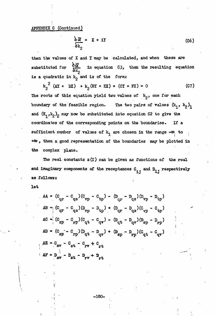
APPENDIX C (Continued)

cz x+jy (c6)

then the values of X and Y may be calculated, and when these are

substituted f or in equation C3, then the resulting equation sç is a quadratic in k and is of the form:

Ic22 (A! + + k2 (BY + El) + COY + 0 (ci)

The roots of this equation yield two values of k2 , one for each

boundary of the feasible region. The two pairs of values (1c1 , ic2 )1

and (iç,ic2 )2 may now be substituted into equation 02 to give the

coordinates of the corresponding points on the boundaries. If a

sufficient number of values of Ic1 are chosen in the range - to

9W, then a good representation of the boundaries may be plotted in

the complex plane.

The real constants z (I) can be given as functions of the real

and imaginary components of the receptances C and Dii respectivelyij

as follows:

let

AA (C qr

-c qs )(o vp -C )-(D tp -D )(D vp qs -D ) tp qr

AB •

(C qr -C qs )(i vp -D )+(D tp qr -D )(c vp qs -c ) - tp

AC - (c - Crp)(Cqt - Cqv) - qt - Dqy)(D5p - Drp )

op.- rp qt qv op rp qt qV

,AEC 5v

-c at -C rV +0 rt

l AFs DOT _D_D+D

- -180-

APPENDIX C (CONTINUED)

and.K(i)a(C - C

)(Cap )-(D -D )(D:-D ) qr qs sp rp qrqs ap rp

x(2)= (a -a )(c -a )- CD -D )(D -D ) qt q7 Yp tp qt q yp tp

K(3)=AEx (AL + AG) -AFX (AB +AD)

K(b)CBS +Crr -Ci's - Car

- 2 - AE

K(6)=C+Ctt- C,-

L(1)-(C -c )(D D) CD -D )(c - a) qr qa Sp rp qr•qs sp rp

L(2) - (a - a )(D D) + (D - Dqv)(Cyp - qt qv vp t qt

rL(3)afi.Ex. (AB + AD) +APx (AL +AC)

LCIiflD38+Drr_ Drs _Dsr

L(5)-2 xAEx'AF

vv. tt Then

a K(1)

= K(2)

- K(1)K(6) - • L(1)L(6) + x(2)x(4) - L(2 )L(4) -. C3)

Z(U) - L(l)

• Z(5) - L(2) •

z(6) - K(1)L(6) + L(])K(6) + K(2)L(4) + L(2)x(4) - LC)

z(7)-x(li)

Z (8) K (6)

z(9) = IC(4)K(6) - L(4)L(6) -

z(iO)-L(U) •

Z (n) - L(6)

- x(4)L(6) + L(4)K(6) - L(S)

• H -'a'-

Muss values

3

m2 10 m3 20

5

All units are compatible

0.5

0€

APPENDIX D

The Nass,Spring.Dpphpot System Used in the Calculation

Of feasible Response Region Botñdaries.

—182-

oximation value

['p

APPENDIX E

The G1aph ofF Against X for an Air Spring AP0 1

-183-

A L

to

0.5

1.5

F 2Af

APPENDIX F

raising and lowering screw •1 rigid mounting wall

fffR:;P)a*t;,, S US

passes through sliding clamp to locate in the retaining block

bea sliding clamp

retaining block

;~ (Inserts into main

Details of the Clamped C antilever Spring. -

—184-

• APPENDIX 0

Output from the Structural Manipulation Program.

***SYSTEM ( 400)***

• ****MODEL OF EXPERIMENTAL SYSTEM USING BLOCK 30/5/75****

***DATA FROM LAST RUN*** FREQUENCY : 2.000@ 2 HZ EXAM,FORCING: 2 6

CHOICE:CIRCLE

DR:2 05:3

**RESPONSE CIRCLE FOR VARIABLE STIFFNESS**

EXAM/FORCING : 2 6 SPRING COORDS : 2 3

FORCING FREUU 2.00000@ 2 HZ RADIUS : 9.58097@ -6 MIN RECEPT MOD : 1.02635@ -4 CENTRE OF CIRC :-1.12215@ -4 , 3.88173LS -7 C[1ORDS AT K=O :-l.10444@ -4 , -9.02773@ -6 COORDS AT K=INF:-1.12774@ -4 p -9-17646@'-6 K AT MIN RECEPT: 4.23910@ 2 COORDINATES :-1.02634@ -4 , 3.55031@ -7

CHOICE: -

Data Concerning the Response Circle for a Single Variable - • • Parameter.

-185-

APfl2iDIX C (continued)

CHOICE :ASSESS

22 SELECTED PARAMETERS

FREQUENCY 2.0004 2 HZ EXAMj.FORCING: 2 6

**STIFFNESS PARAMETERS**

** EL EM EN T ANALYSIS BASED ON ASS OC IATED PARAMETERS**

LOG SCALE

MINIMUM CIRCLE

B IAS EL EM RESPONSE ELEM DIAMETER ELEM CIC ARC

I) I

1.0@ 0 8 1.0@ 0

I.0@ 0 8

3.0 -1 1 3.6@ -I

8 1.00 0 2 2.5@ -I 2 3.0@ -2

2 8.7t -1 9 2.54 -i 9 2.44 -2

9 7.9w -t 3 2.4@ -1 13 2.3@ -2

3 6.14 -1 10 2.30 -I 6 2.I® -2

6 5.4w -1 4 2.3 -1 12 2.0 -2

13 5.34 -1 II

2.3@ -1 3 I.7@ -2

10 4.3@ -1

9). 6 2.8@ -2 10 I.2@ -2

11 3.14 -1 -

10) 13 2.5@ -2 4 9.2@ -3

4 3.14 -1

II) 7

9.4@ -3 11 9.2@ -3

7 2.64 -I 14 7.2@ -3 7 5.9@ -3

14 2.04 -I 5 1.0@ -3 14 4.3@ -3

12 3.64 -2 12 0.0@-99 S 0.0@-99

S 0.04-99

PR INTOUT?: N

CHOICE:

I Effectiveness Criteria for a Single Variable Stiffness Parameter.

- t -186-

APPENDIX d (Continued)

CHOICE :ASSESSALL

PARAMETER SELECTIONS ALREADY MADE

***ZERO RESPONSE USING TWO STIFFNESS PARAMETERS***

22 SELECTED PARAMETERS 253 POSSIBLE PAIRED COMBINATIONS 43 PAIRS GIVE ZERO RESPONSE

ELEM LISTflY

FREQUENCY 2.000@ 2 HZ EXAM/FORCING: 2 6 -

OCCURRENCE OF ELEMENTS BASED ON SUCCESSFUL PARAMETERS:-

PARAMETER BREAKDON

• ELEM NORM TOT, X Y 1 TI T2 T3

1) 11.00 24 3 0 0 0 21 0

• 2)20.52 133 00 0 10 0 60.35 9 0 0_U 0 9 0, 80.26 1 3 0 0 0 4 0 90.22 6 3 0 0 0 3 0 30.13 4 3 0 0 0 1 0 40.13 4 3 b •o cx i a 50.13 4 0 0 0 0 4 0 100.13 4 3 0 0 0 I 0' 110.13 4 3 0 0 0 I 0

ii) 120.13 4 0 0 0 4 0

• 12) 7 0.00 1 0 0 0 0 1 A)

13)130.00 1 0 0 0 0 I 0

14) 140.00 1 0 0 0 0 1 0

PRINTOUT?: Y HOW,MANY:2

DR DS UT, Dv COORDINATES 2'G '. 26

I.0000000000@ 35 1.1221374573@-14 -2.111'-20 -8.470-22 9.5432030276@ 18 5.06365646344 2 3.3884-21 0.0004-99

- 2 G 3 , 4 4.99161151474 18 5.11546325164 2 -1.1624-19 1.0864-19

- 1.3351891932419 1.91440694634-13 1ST NG

ANY MORE?:N

Assessing for Zero ReSDonse Using Two Parameters. -18'I-

The Transformation Matrix used in the Mathematical Model

to Account for the Finite Size of Structural Nodes.

Z

t

4

87

N

Figure Hi

Finite Element AB and Rigid Extensions CA and BD

Figure lii represents a simple finite element beam A3 with

rigid extensions CA and RD of length 0.575". Considering the left

hand end of the bean, the transfrnation between the coordinate àystea a

at points A. and c is:

1 0

- 0 0.975 Y2

0 0 1 0 -0.8750 Z 2

• 00 0

0 0 0 0 1 0

0 0 0 0 0 1 *2

-188-

APPENDIX fl (Continued)

or in matrix notation:

! (a) ma relationship between the forces in the two coordinate system is given by:

* T (112),

where AT is the transpose of

For the right hand end of the beam:

10 0 0 0 0

71 0 1 0 0 0 -0.875 721

0 0 1 0 0.8750

0.o 0 . 1 0 0•

01 0 0 0 0 1 0 6.21

01 0 0 0. 0 0 1 021

or, in matrix notation

laX -r -r -r R3

The relaticiship between the forces in the two coordinate system is -

F * CAT F -r -r -r (Hh

The relationship between the forces and displacements for the element is:

FaKX

where

FL 1

-

[Fr J 1Ix- [K2T I

LXr K3J

Substituting for F, F, It and I from equations 111, 112, 113 and u1 gives

• -180- -

APPENDIX H (CCt4TDnJED)

where.

rFrL LrJ

and - $j2Xr

?K3AJ which provides a relaticnship between the forces and displacements

at points C and D on the beam.

The Constants Involved in Calculating the Feasibility of a

Desired Response.

For a single stiffness parameter Ic the response at a point

in the structure is given by:

e+if+ k(a+ib) (ii)

1+k (c+id)

where, a, b, c, d, e and £ are real constants and are defined in

Appendix A. The real and imaginary components of a area

u e+k(a+k(ac+bd) (12).

1 + 2ck + k2(o2+ 42)

• v - f +Ic(b +k(bc - ad)) (13)

1 + 2ck + k2 (C 2 + d2 )

respectively. Now ja 1 may be written:

Bk (iJ)

P1c2 +Qk+.R

where A (a2 + b 2 ) + (e2 + f2)(c2+ 42) + 2e(ac + bd) + 2f(bc -d

• • B 2c(e2 +f2 )+2(fb +ea)

• •C e2 +f2 -

• P- c2 +d2 .

Q 2

Ha-i •

• •.. •

• -191-

APPENDIX x (Continued)

The first derivative of k 1 2 with respect to Ic is

.- kl 2 _k2 (_)+ 2k (RA PC) +(RB QC) (IS)

dIr (pk2 +Qk+ B)2

and the second derivative of k 2 with respect to Ic is

d2 1I 2 - g1 (k)- a2 (k)

a3 (Ic)

where

a1 (k) - 2(Pk2 + a + R)2 (k(QA - PB) + (RA - BC))

- 2(k2(QA - p) + 2k (RA - p0) + (u - QC)) P1c2 + a + B)(2Pk + q)

o(k)- (pj2 + a

-192-

APPENDIX J

Data Used in the Preparation of the Mathematical Model.

efer to Figure 6.16.

Stiffness Elements.

Second Moment of Area.

Y— lvll

I bcI3 - l x (0.063) a 2.083 x YY if 1075 in.4

12

Element lengths

Elements 5,6,7 212 313 and 14 = 6"

Elements 1,2094,8,9 and 10 4"

Young's Modulus.

Young's Modulus was determined experimentally by measuring

the tip deflection of one of the a'ing steel beams comprising the test

structure.

For a beam, length 5", the tip deflection wider a loth

of 1.2 lbs. was .0905".

From simple beam theory

125x1.2x 10 - 2.6524x107 lb/In.2 31x 3 x 2.083 x 0.0905

H —193-

APPENDIX J (CONTINUED)

The added stiffness of the variable stiffness element.

The variable stiffness element is a simple cantilever of

maximum length 4.6". (This remained constant during the measurement

of natural frequencies and mode shapes). The stiffness at the tip

of this element is given by:

k- 3E1 V

Thus Ic = 3 x 2.65 x 10 x 2.083 x 10 17.0 lb/in

(b.6)

This value was added to element k(1,1) In the structure stiffness matrix.

The stiffness matrix of the mathematical model of the test

structure is as follows: (units lb/in.)

81,4.9 0 0 0 0 297.5 297.5 297.5

2539.4 368.5 0 0 7174 0 0

3091.9 368.5 0 0 717.5 0

3091.9 368.5 0 0 717.5

SIX 2539.14 \ 0 0 0

1545.9 368.5 0

2098.1, 365.5

2098.0 -

In order to determine the accuracy of this data, the stiffness

of the test stra,ture in the horizontal 'direction at node 5 was

determined experimentally. A horizontal load of 10.2 lb. was applied at

this pqint, and the corresponding deflection was found to be 0.011,".

Thus, the stiffness at that point was:

10.2 728 Win.

0-014

-194-

APflNDIX j (CONTINUED)

To obtain the equivalent term from the theoretical stiffness matrix,

consider the matrix in the partitioned form

[?j

[k]. k21 61

I-I (.ii)

L4J• L2 where F1 is the force 1n the x direction of node s and çthe corresponding deflection.

• !2 , 3 and 2 are of the order (lxi)

is (1 x7)

• kbis(7 x7)

We require to know the deflection 6 for F - lib. and F - 0 -

1 1 Now., if if equation Ji is expanded, then

• F1 - k161+ k22 (J2) -•

• Therefore,

á2 l4-1 k3 61

which ml- be substituted into equation (J2) to give

F1 - -

Thus, the required stiffness term is

-1 • Ic_ 2Ij -.3

When these terms are calculated from the stiffness matrix given above ,

then the following valvB is obtained:

184409 - 1231 721.9 lb/in.

This corresponds favourably with the value of 728 lb/in. .obtaithd

experimentau,y. - • . -•

-• i • • -195-

APPENDIX J (CONTINUED)

Mass and Inertia Data.

The mass of the structure in the direction corresponding to

degree of freedom 1 canprises the total mass • of four blocks, three

beams and associated accelerometers and couplings. This value was

measured experimentally and found to be

1.8 x 1072 lbt in'seC'

Figure Ji • shows one of the structural node blocks

a- .

z.- .

a-

Figure J.1 J.1.

Structural Node Block

The moment of inertia of the block in then direction is given

W the equation

ff zz

I 12

Now the We5.at of each block was found to be 1.8 lbf and La. 145",

therefore &

- —196-

APPENDIX J (CONTINUED)

2 x 1.8 x (1.75)2 - 2.377 x 10 lbç in.Se& zz

12 x 32.2 x 12

The moment of inertia of an accelerometer mounted as shown in

Figure 6.15. about the zz axis Is

0.056 x 10 lbci.SeC

Thus, the total inertia of the block plus accelerometer Is

2.426 x lO lbFin.SEC

This value was adjusted according to the amount of additional

instrumentation on any given block. The following were the initial

estimates for the :inertia data.

Block Inertia lbçln.SeC'

1 2.5x10 3

2 2.145 x 10

3 2.12xl0 3

4 2.42x1073

5 2.5z].0 3

6 2.42 x.10-3

7 2.142x1073

The inertias of inditdual blocks were not determined experi31entafl,y.

—Y

t 1 • .

APPENDIX K

The Stiffness Matrix for a Linearly Tapering I Beam.

I

di fl1%rd tuper ruitu i

b

• H 1=1= btd ° yy 2

Figure Li.

The stiffness matrix for the beam shown in Figure Li • may be

obtained using standard techniques and is given overleaf.

• -198-

rl

APPINDIX K (CONTINUED)

+ 1c2 (ê-x2 ) k2 (L-x) k2 (€x Ic - x2)_, -k2 (L- x)

Ic2 k2

Ic1 + k2x2 -k2x

Ic2

when

k1 1 (r+1w*1Or2 +hr+1)

(2r2 +r+2)

k2 12 (2r2 +r+2)

St 2

and z Q. (17r+6r+ 7)

12 (2r2 +r+2)

I

-199-

Newman, K.W.

Simpson, A.

Vincent, A.H.

Bishop, R.E.D. and

Gladwefl, G.M.L.

Spiegel, M.R.

Sneddon, I.N.

K3rra], A.

sussh6lz, B.

Thompon,

Gaukroger, D.R.

Skingle, C.W. and

Heron, K.H.

Predicting the Effects of Parameter

Changes in Dynamical Systems.

RAE T.R. 69142 (A-R-C 32597) July 1969

Zigenvalue and Vector Sensitivities in

Kron 's Method. Journal of Sound and

Vibration (1973)31 (1),73-87.

A Note on the Properties of the Variation

of Structural Repponse with Respect to a

Single Structural Parameter When plotted

in the Complex Plane. GEN/rN,4tES/O1OR

Sept. 1973. (Unpublished Westland Helicopters

"Report)

An Inve1tigation into the Theory of

Resonance Testing. Phil. Trans. Roy. Soc.

Series A,No 1055,255 January,1963.

Theory and Problems Of Complex Variables.

Schaums Outline Series. McGraw-Bin, 1964.

Elements of Partial Differential Equations.

McGraw-Hill, 1957.

Applied Functions of a Complex Variable.

Wiley-Interscience, 1972.

Forced and Free Motion on an .Airspring.

Journal of Applied Mechanics, June 194,101-107.'

Vibration Theory and Application. London 1966.

Numerical Analysis of Vector Response Loci.

Journal of Sound and Vibration (1973)29(3),

3L1-353.

-200-

(fl) Milne, R.D. and Reconciliation of Calculated and Measured

Simpson, A. Natural Frequencies and Normal Modes.

Journal of Sound and Vibration (1973)30(1),

1&5-63.

Marples, V. The Derivation of Modal Damping Ratios

from Complex Plane Response Plots.

• Journal of Sound and Vibration (1973)31 (1),

•

105-17.

Nottingham Algorithms NAG mini Manual for the NAG I3 360-370

Group. Library, 1973.

(lit) Pestle, LCE. and Matrix Methods in flastomechenics.

Leckie, F.A. McGraw-Hill, 1963.

Jenkins, W.M. Matrix and Digital Methods in Structural

N Analysis. McGraw-Hill, 1969.

Sciarra, J.J. Application of Impedance Methods to Helicopter

Vibration Reduction. Paper Presented at

Imperial College London, July 1973.

Sciarra, J.J. Application of Combined Direct Stiffness

and Mobility Methods to Vibration Absorber

Studies. American Society of Mechanical

Engineers. 67-VIBR-65, 1967. -

Scidrra, J.J. Helicopter Fuselage Vibration Prediction

by stiffness Mobility Methods.

The Shock and Vibration Bulletin. (1968)37

(6),19-28.

Woodàocfr, D.L. The Rate of Change of EigenvaJ.ues of a

Lambda Matrix and Their use in flutter

Investigations. Journal of Roy. AerO. Soo.'Y.

(196070064-365.

-201-

Kron, G. Diakoptics.

London MacDonald & Co. (1963).

Narramore, C.H. A Theoretical Investigation of Systems

Designed to Isolate the Fuselage of the

WG.13 Helicopter from the Effects of Rotor

Induced 14R Vibration. Westland Helicopters

Ltd. Report. WG.13/DIN/001R.

Den Hartog, J .P. Mechanical Vibrations. 14th DL McGraw-Hill,

Ney York, 1965.

Paul, W.F. Development and Evaluation of the Main Rotor

Bifilar Absorber. 25th Annual National

Forum Proceedings of the Americal Helicopter

Society. (1969).Paper No 3514.

(214) flanne].14r, W.G. Dynamic Anti-Resonant Vibration Isolator.

U.S.A.. Patent No 3,322,379 (1967).

Venkayya, V.B. Design of Optixrxtra Structures. Computers

and structures ) ,Vol 1 (1971) 2 265-309.

Turner, M.J. Design of Minimum Mass Structures with

Specified Natural Frequencies. AIli Journal

(1966)Vol 5 1No 3,1406-412.

Ellis, D.V. . Structural Optimisation Applied to the

Helicopter Vibration Problem. ARC 351148, (19714).

Barnard, A.J. . Helicopter Structural Analysis Uslpg

-.

McLaughlin, A NSC/tASTRAN . Users Conference, Munich 1975.

Webby,\J.P, and

taker, T.

Taig, I.C. and Optimisation of Aircraft Structures with

• Keri, R.T. Multiple Stiffness Requirements.

AGARD, 2M symposium on Structural optimisation.

(1973).

-202- .

(yo) Rubin, C.P. Dynamic Optimisation Of Complex Structures.

AIAA Dynamics and Aerolasticity Specialists

Conference, New Orleans, La(April, 1969).

I / -

K -203-

PUBLISHED WORK

I

Done, G.T.S. and The Response of a Vibrating Structure -

Hughes, A.D. as a Punction of Structural Parameters.

Journal of Sound and Vibration (1975)(2),

255-266.

• N

'I

Ii

N N

Journal of Sound and Vibration (1975) 38(2), 255-266

THE RESPONSE OF A VIBRATING STRUCTURE AS A

FUNCTION OF STRUCTURAL PARAMETERS

0. T. S. DONE AND A. D. HUGHES Department of Mechanical Engineering,

University of Edinburgh, Edinburgh EH9 3.JL, Scotland

(Received 14 May 1974, and in revised form 13 August 1974)

The response of a structure excited by an external oscillatory force is examined for variations in certain structural parameters of the system. This is done with a view to manipulating the structure in order to achieve a desired response. The variation of the response with one structural parameter is seen to be simple, and the effect of changing in addition the forcing frequency is illustrated. When two structural parameters are con-sidered, it is seen that a desired response may or may not be attainable, as defined by a "feasible response region". The application to practical cases is discussed briefly.

1. INTRODUCTION

Linear structural analysis is now a relatively straightforward task, and has been greatly aided in the recent past by the advent of digital computers. However, the results of an analysis can be so large in quantity and extent that in the case of a vibration problem producing unacceptable results the answer to the question "How does one alter the structure to produce the originally desired dynamic characteristics?" is very far from evident. Small perturbation analysis exists [1,2] which goes some way towards providing an answer and, of course, it is possible to make use of one of the many computer based formal optimization routines. Neither of these is entirely satisfactory; in the former case it may be that gross rather than small changes in the structure are needed to achieve the desired results, whilst in the latter, although it is possible to effect a gross change by a succession of many small ones, the dis-advantage of the process being heavily computer orientated remains.

The reason why a heavy reliance on the computer is not altogether satisfactory in the present problem is because of the lack of freedom of action to change parameters following the assessment of some subsidiary analysis: that is, to change the parameters in a non-predetermined manner. In a formalized optimization the parameters are changed in a pre-determined way dependent on the mathematical method, the constraints and the objective function chosen. The knowledge that is a necessary prerequisite in allowing the above-mentioned freedom of action is really the same thing as "feel" or "insight".

It is not only in dealing with the mathematical model of a structure that insight is valuable. When the vibration performance of a newly assembled structure is not up to expectation or specification then the integrity of the mathematical model used for the design is rendered uncertain, and the model itself may not be used as a means of finding suitable modifications. In such a situation in practical engineering any modification suggested by a dynamicist (who at this stage would be under considerable pressure to produce a satisfactory solution) is likely to be the result of fairly simple calculations, which provide some insight, and past experience. More insight at an earlier stage would have placed the dynamicist in a better position to be able to suggest modifications; he might, for instance, have known in advance which parts of the structure are most effective in controlling unwanted vibration.

255

256 G. T. S. DONE AND A. D. HUGHES

The above preamble provides the justification for the present work which arises from the desire to know what are the effects on the dynamic properties of a structure resulting from a gross change or changes in one or more structural parameters. The particular aspect examined was stimulated by the necessity in helicopters to keep the rotor induced vibration levels in the passenger and pilot area of the fuselage down to a minimum. The helicopter problem has been used as a basis for the simplified model employed in this work. In this model, a linear structure is subjected to a single oscillatory force and the effect of changing one or more structural para-meters on the response at some point on the structure is examined. The structural parameter itself is idealized by using a simple spring, and the examples used in calculations are simple mass, dash pot and spring systems. The theory for this model follows on the lines of that established by Vincent [3].

2. RESPONSE AS A FUNCTION OF ONE STRUCTURAL PARAMETER

2.1. SINGLE DEGREE OF FREEDOM SYSTEM Although it is of little importance practically, an initial appreciation of the behaviour of a

simple one degree of freedom case is helpful in examining more complicated systems. The equation of motion of a single degree of freedom system subject to harmonic excitation

at circular frequency co may be written as

mi+L±+kx =Febot, (1) (1)

where m is the mass, k the stiffness and F the magnitude of the excitation. The damping, represented by the coefficient h, is considered to be hysteretic for reasons of simplicity in the following analysis. The steady-state solution for the response is

x = G((o) Fe",

where

17 (2)

(k - mw') + ih

and is the complex receptance of the system. It is well known that the locus of the end of the vector G(w) on the complex plane as o varies is a circle of diameter 11h passing through the origin and with its centre on the negative imaginary axis [4]. Figure 1 shows the response circle appearing as a projection from the three-dimensional locus of 6((0) produced by including w as one of the co-ordinates. Part of the circle is not physically realizable as it corresponds to 0)2 <0 (shown dashed in the figure).

The circular locus arises by virtue of the variation of the real part of the denominator (k—mw 2) in the right-hand side of equation (2). Thus, a variation of k or m, or indeed k, m and w2 in proportional amounts, leads to the same locus. By considering the signs of k, in and 02 in the term (k - ma?) it is seen that the end of the receptance vector 6(k) ask increases, m and w2 being held constant, traces out a circle in the opposite direction (i.e., anti-clockwise) as that for increasing 0)2 and m. The effect of varying the damping coefficient his illustrated in reference [4], in which 6(h) is seen to produce a circle whose centre lies on the line of the real axis.

If the circles representing G(k) are plotted in three dimensions as in Figure 2 for all values of w, then a circular cylindrical envelope is developed. Those parts of the loci corresponding to negative k are shown by dashed curves. On the envelope, curves of constant k can be plotted as indicated, these being of the same type as that in Figure 1.

RESPONSE OF A VIBRATING STRUCTURE 257

6(w)

Increasing

Figure 1 Response as a function of frequency.

Thus it may be seen in the simple case of a one degree of freedom hysteretic system there is a straightforward relationship between the complex response as mass or stiffness varies and the more familiar response as frequency varies.

2.2. MULTI-DEGREE OF FREEDOM SYSTEM

As in the single degree of freedom case it is convenient to express the responses of the system by means of receptances. These follow from consideration of the equations of motion which

Gtk)

Increasing 4

Figure 2. Response as a function of stiffness and frequency (one degree of freedom).

258 G. T. S. DONE AND A. D. HUGHES

may be written as

M+C+Ki=Fe', (3)

where M, C and K are the mass, damping and stiffness matrices, respectively. F is a vector of force amplitudes and K is a vector of time-varying structural displacements. The system is considered subject to harmonic excitation at circular frequency CO and since no particular advantage is now to be gained by using hysteretic damping, the damping is assumed to be viscous. The steady-state solution for the response is R = xe iwt where

= GF

(4)

and G=[K—Mco2 +iwC]'. (5)

The system to which these equations apply is shown schematically in Figure 3. It represents a structure having many degrees of freedom for which it is required to examine the response at the material point q due to a single forced excitation at point p.

Figure 3. Structure and variable stiffness spring.

A simple structural modification is made by inserting a linear spring of stiffness k between two points r and s that have mutually compatible degrees of freedom. The spring is adjusted so as to exert zero force when the system is in equilibrium. When the original structure is considered as a free body, the forces exerted on it at points r and s by the spring are F, and F,, respectively, which have the relationship

F,=k(x,—xj=—F,. (6)

The forcing vector F in equation (4) contains three non-zero elements, F,, F, and F,,, whereas the elements of immediate interest in the response vector x are Xq, X, and x,. Partitioning and expanding equation (4) yields

xq =Gqp Fp +Gq,F;+G45 Fs, (7)

in which G,3 is the complex receptance providing the displacement at point i due to a force at pointj.

RESPONSE OF A VIBRATING STRUCTURE 259

The forces Fr and F may be expressed in terms of X and x, by using equation (6) and subse-quent elimination of x, and x, gives

xq k(G3 - Gr,)(Gqr - Gq,) (10)

F, - = Gqp

+ 1 + k(Grr + G. - G, - G)

This is now the modified complex receptance between points q and p in terms of k and the original complex receptances G,. In turn, it may be rewritten in more general terms: i.e.,

C = + in

k(a + ib)

=(e+ if) +k(d) (11)

where C xe/F,, and a, b, c, d, e and fare all real. It can be shown that ask varies from - to +w the locus of the tip of the complex receptance

vector, C , traces out a circle in the complex plane (see Appendix A), the equation of the circle being

b ]'+[, _ (f_ \12 2

an a-I- b2

)i __4d­2_' (12)

It is worth noting here that the co-ordinates of two important points on the circle, namely k = 0 and k = co, are

k=O: [e,f],

(ac +bd)(bc— ad) ] k = : [e + c2+d2 f+.c2+d2 f

These points bound the arc of the circle containing negative values of k. Strictly, if k is associated with a real spring then this part of the circle is not physically realizable. However,

Figure 4. Response as a function of stiffness and frequency (several degrees of freedom).

260 G. T. S. DONE AND A. D. HUGHES

it is possible to consider negative k as subtracting from existing structural stiffness and in this case the Situation is physically attainable whilst the overall stiffness matrix remains positive definite: i.e., whilst static stability is maintained. Of the two possible arcs, that which is associated with negative k may be determined from the direction of the locus with increasing k. This can be shown to be anti-clockwise for the negative values of the constant din equation (11) which invariably have been found to occur in practical cases. As with the single degree of freedom case it is possible, by introducing forcing frequency as a co-ordinate, to construct a surface corresponding to a given stiffness parameter upon which the three-dimensional response curve can be drawn for various values of that parameter. Figure 4 shows the pictorial representation of a typical surface, the response for the curve corresponding to k = 0 being projected below on to the complex plane (the latter is often referred to as a Kennedy—Pancu plot). Information concerning the system from which this surface was generated is given in Appendix B.

3. RESPONSE AS A FUNCTION OF TWO STRUCTURAL PARAMETERS

3.1. FEASIBLE RESPONSE REGIONS

As in section 2.2 the response at a point q on the structure due to a force at pointp is sought. Two variablespring elements of stiffnesses k 1 and k2 are connected between points r,s and t, v, respectively, where

F, = k1 (x, - x,) = —F,, F k2(x, - x,) = — F,. (13)

Equation (4) again can be utilized to give the relevant equations:

Ii=q,r,s,t,v xg =Gjj Fjj I. (14)

J j=p,q,r,s,t,vJ

Substituting for F,, F,, F, and F in equations (14) and eliminating x,, x,, x and x gives the following equation:

XQ Gqp + k1 4' 1 (k,) + 02(k 2)

-= (15) k 1 (k 2) + 04(k 2)

where the (k,) are complex linear functions of k 2 and are given in Appendix C. It may be seen that the form of this equation when k2 , say, is held constant whilst k 1 is allowed to vary

In,

Figure 5. Response circles for two structural parameters.

RESPONSE OF A VIBRATING STRUCTURE 261

is similar to that of equation (11). Thus, in this case a circular response locus is produced. When k2 assumes another value, another circular response locus is obtained as k 1 varies. If the k 1 circle is "started" at the same value of k 1 each time, then these starting points lie on the response locus of the system when k 2 alone is varied (see Figure 5). By covering all possible combinations of k 1 and k2 a region in the complex plane is formed inside which the response at point q due to an oscillatory force at p must lie. This is referred to as a "feasible response region". Figure 6 shows an example. As in the single varying parameter case, some parts of

Figure 6. Feasible response region from response circles. Details of system given in Appendix B. Dashed line indicates negative stiffness.

the region violate the physical requirement that the overall stiffness matrix must remain positive definite. Details of the system used in the examples are given in Appendix B.

An alternative formulation of the problem, which relies on the use of matrices, is given in Appendix D. Any number of structural parameters can be considered, but so far no attempt has been made to apply the theory to a practical example.

3.2. THE BOUNDARIES OF THE FEASIBLE RESPONSE REGIONS

The boundaries of the feasible response region are given when the Jacobian, a(, )1a(k 1 , k 2)

is zero [5] i.e.,

ac/ak, /dkI a1/ak, a1/akj°' (16)

or, alternatively,

Im ac (17) ( \

=0

where dQak2 is the complex conjugate of ac/ak2 and C= + iq x/F. Equation (17) is found to be of the second order in k 1 and k 2 and the possibility of two

boundaries exists. At any point on these boundaries the values of k 1 and k2 are uniquely

(n

k,•)

(c' (cfl

262 G. T. S. DONE AND A. D. 1-LUOI-IES

Figure 7. Typical feasible response regions.

defined, whereas within the region it may be observed from Figure 6 that there are two sets of values (k 1 ,k2) corresponding to each response point. Figure 7 gives some examples of typical feasible regions obtained by direct solution of equation (17) following the appropriate differentiations in equation (15). The systems concerned again are defined in Appendix B.

4. DISCUSSION

The mathematical models considered in the present work are idealized and, although there is presumably a certain intrinsic academic interest in the results, it remains to be seen how useful the theozy would be in a practical case. In most practical cases of manipulating a structure to produce a desired vibratory response the aim would be to minimize the response over all or part of the structure. (An exception to this would be changing a normal mode shape on an aircraft wing, say, for the purpose of changing the aerodynamic generalized forces and thence the flutter characteristics.) In the present formulation, with not more than two spring variables, the minimum response (if zero is not a feasible response) could be obtained uniquely by using the equation of the outward normal to the boundary with no recourse to search techniques. When zero response is feasible, i.e., when the feasible region surrounds the origin, there is a choice between two uniquely defined sets of variables.

In practical applications one of the problems is to choose the regions of the structure in

RESPONSE OF A VIBRATING STRUCTURE 263

which a change of structural parameter or parameters is most effective. In such applications of the present formulation it is proposed, initially anyway, to use the relative magnitude of the response circle for a single parameter as a measure of effectiveness. In this connection, it should be noted that the systems discussed in this paper are not meaningful in any numerical sense, but have been used only to illustrate in the most general way the variation of the response. As the main purpose of this paper is to draw attention to some of the more interest- ing phenomena, the discussion here is confined to outlining some of the difficulties expected in practical applications.

Another problem is to obtain a transformation between the ideal springs considered as structural parameters and the geometric parameters, (which would affect mass as well as stiffness), such as skin thickness, tube wall thickness, beam web depth, etc., that would be used in practice. This also is a difficult area when one is using the more conventional optimiza-tion methods because the mathematical equations of motion of vibration systems are usually expressed in terms of variables other than the geometric parameters: e.g., generalized co- ordinates.

The direct application of the present work to simple and more practical examples of structures is in progress, and will be reported on in due course.

ACKNOWLEDGMENTS

Thanks are due to several people at Westland Helicopters Limited for providing the stimulus for this work and for their continued encouragement and assistance.

REFERENCES

I. K. W. NEWMAN 1969 (July) RAE T.R. 69142 (ARC. 32597). Predicting the effects of parameter changes in a dynamical system. - A. SIMPSON 1973 Journal of Sound and Vibration 31, 73-87. Eigenvalue and vector sensitivities in Kron's method. A. H. VINCENT 1973 (September) Westland Helicopters Ltd. Report GEN/D YN/RES101OR. A note on the properties of the variation of structural response with respect to a single structural parameter when plotted in the complex plane. R. E. D. BIsHoP and G. M. L. GLADWELL 1963 Philosophical Transactions of the Royal Society London, Series 4,255, 241-280.. An investigation into the theory of resonance testing. I. N. SNEDDON 1957 Elements of Partial Differential Equations. New York: McGraw-Hill Book Company, Inc. A. KYRALA 1972 Applied Functions of a Complex Variable. New York: Wiley-Interscience.

APPENDIX A

It is required to find the nature of the complex equation

k(a + ib) (=(e+ if) + +

k(c+ id) (Al)

as k is varied between -w and w. Let C = + i,1. Then

a + ib (-e)+i(,j-f)= (A2)

(1/k) + c + id

giving

(l/k)+c+id= (a+ib)(( -e)-i(j-f))

(A3)

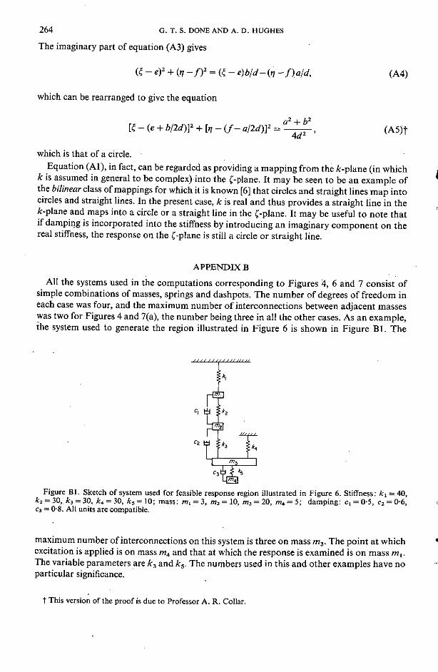
264 G. T. S. DONE AND A. D. HUGHES

The imaginary part of equation (A3) gives

( - e) + (q -f) 2 = - e)b/d—( —f)a/d, (A4)

which can be rearranged to give the equation

[—(e+b/2d)]2 + [q—(f—a/2d)] 2

= 4d2

a2 + b2' (A5)t

which is that of a circle. Equation (Al), in fact, can be regarded as providing a mapping from the k-plane (in which

k is assumed in general to be complex)into the (-plane. It may be seen to be an example of the bilinear class of mappings for which it is known [6] that circles and straight lines map into circles and straight lines. In the present case, k is real and thus provides a straight line in the k-plane and maps into a circle or a straight line in the c-plane. It may be useful to note that if damping is incorporated into the stiffness by introducing an imaginary component on the real stiffness, the response on the (-plane is still a circle or straight line.

APPENDIX B

All the systems used in the computations corresponding to Figures 4, 6 and 7 consist of simple combinations of masses, springs and dashpots. The number of degrees of freedom in each case was four, and the maximum number of interconnections between adjacent masses was two for Figures 4 and 7(a), the number being three in all the other cases. As an example, the system used to generate the region illustrated in Figure 6 is shown in Figure Bl. The

fri

C1 k2

C2 3;;

Figure El. Sketch of system used for feasible response region illustrated in Figure 6. Stiffness: 40, k2=30,k3 =30, k4 =30, k5 =10; mass: m 1 =3, in2 = 10, "13 =20, "14=5; damping: c 1 =05, c2 =06,

= 08. All units are compatible.

maximum number of interconnections on this system is three on mass in3 . The point at which excitation is applied is on mass in4 and that at which the response is examined is on mass m 1 .

The variable parameters are k 3 and k5 . The numbers used in this and other examples have no particular significance.

t This version of the proof is due to Professor A. R. Collar.

RESPONSE OF A VIBRATING STRUCTURE 265

APPENDIX C

The equation for the complex responses x0/F, as a function of two variable spring parameters k 1 and k2 is given generally by

k 1 0 1 (k 2) + 4 2(k 2) C_Gqp+ (Cl)

k 1 4;(k2) +

where q and p refer to examination and forcing co-ordinates, respectively. The functions 4,(k 2) are

4 1 (k 2) = a1 b1 (l + k 2 c22) + a2 b2 c11 k 2 - k 2(a2 b 1 c21 + a1 b2 c12), 02(k 2) = a2 b2 k 2 ,

= c0 +k2c22) - C21 q2 k2,

4 4(k 2) 1 + k2 c22 1

where a,, b, and Cu are the complex elements of matrices A, B and C in Appendix D. These elements are functions of the complex receptances Gjj and are given by

a1 = Gqr - Gqs , a2 = G, - GqT b i = G, - Grp, b2 = GE,p -

= C,, + C5. - C,. - C,,., c12 = G, - - Grv + G,,

= G, - - G + Gtr , c22 = C, + Gvu - - Gtv

where k 1 is connected between co-ordinates r and s and k 2 between co-ordinates t and v.

APPENDIX D

The setting up and reduction of equations (14) to give the single expression for the complex receptance as shown in equation (15) rapidly becomes more complex as the number of variable parameters considered increases. As a consequence of this it is convenient to have a general matrix expression for the complex receptance in terms of in variable stiffness parameters. -

The response at the examination point, q, may be written in terms of the external force, internal spring forces and the corresponding receptances:

Xq = Cqp F + k1 5 1 (G 1 - G.2)+ k2 62 (Gq3 - Gq4)... k m 5(Gq 2m-1 - Gq 2,,i), (DI)

where k 1 is the ith variable stiffness parameter and 5 1 = x21 - x21 _ 1 is the extension of the ith spring (x2 , and x21_ 1 being the actual axial displacements at each end). Equation (Dl) alternatively may be expressed as

X q =Gqp Fp + AKÔ (D2)

where A is a (1 x in) row vector of the terms

- G 2), (G13 - Gq4) 1 . . . (Gq 2m-1 - Gq 2m)},

K is an (m x in) diagonal matrix of the stiffness parameters k, and 5 is an (m x 1) column vector of extensions.

266 G. T. S. DONE AND A. D. HUGHES

The values 61 themselves may be expressed in the same way as x q in equation (DO: i.e.,

61 =F(G2 ,, - G1 ,,) - k 1 b 1 [(G22 - G21 ) - (G 12 - - k 2 t5 2 [(G24 - G23) - (G 14 — a 13)]. -52 = F,,(G4 ,, - Ga,,) - k 1 3 1 [(G42 - G41 ) - (G32 -

6. = Fv(G2m;p - 2m-1, )" km 6.1(G4, 2. - - (Gs , 2. - Gs 2m-I)], (D3)

which can be written in matrix notation as

5= F,, B - CKS

(D4)

Where B is an (m x 1) column vector of terms

- G1 ,,), (a4, - a3,,). ... . (G2m . p - G2.- 1, ,)}

and C is an (in x in) matrix of complex constants in which C, j = (021,2J - G21.2j_l) -

2j - G2 ,- 1• ). An expression for '5 can be found from equation (D4) and substituted into equation (132) to give

Xq =Gqp +A[K- 1 +C]-IB, (D5)

which provides the complex receptance, xe/F,, as a general function of in stiffness parameters.