1

Anti-Aliased 3D Cone-Beam Reconstruction Of Low-Contrast Objects With Algebraic Methods

Klaus Mueller1,2, Roni Yagel1, and John J. Wheller2

1 Department of Computer and Information Science, The Ohio State University, Columbus, OH2 Department of Pediatrics, The Ohio State University, Columbus, OH

Abstract

This paper examines the use of the Algebraic Reconstruction Technique (ART) and relatedtechniques to reconstruct 3D objects from a relatively sparse set of cone-beam projections.Although ART has been widely used for cone-beam reconstruction of high-contrastobjects, e.g. in computed angiography, the work presented here explores the more challeng-ing low-contrast case which represents a little investigated scenario for ART. Preliminaryexperiments indicate that for cone angles greater than 20˚, traditional ART produces recon-structions with strong aliasing artifacts. These artifacts are in addition to the usual off-mid-plane inaccuracies of cone-beam tomography with planar orbits. We find that the source ofthese artifacts is the non-uniform reconstruction grid sampling and correction by the cone-beam rays during the ART projection/backprojection procedure. A new method to computethe weights of the reconstruction matrix is devised which replaces the usual constant-sizeinterpolation filter by one whose size and amplitude is dependent on the source-voxel dis-tance. This enables the generation of reconstructions free of cone-beam aliasing artifacts atonly little extra cost. An alternative analysis reveals that Simultaneous ART (SART) alsoproduces reconstructions without aliasing artifacts, however, at greater computational cost.Finally, we thoroughly investigate the influence of various ART parameters, such as volumeinitialization, relaxation coefficientλ, correction scheme, number of iterations, and noisein the projection data on reconstruction quality. We find that ART typically requires onlythree iterations to render satisfactory reconstruction results.

Keywords: cone-beam reconstruction, 3D reconstruction, Algebraic Reconstruction Tech-nique (ART), Computed Tomography (CT), aliasing

1. IntroductionCone-beam computed tomography (CT) can be thought of as the 3D extension of the widely pop-ular fan-beam CT. It reconstructs a 3D representation of either the entire object or at least a thicksection thereof and is thus a volumetric imaging method. In cone-beam CT, an X-ray point sourcerevolving about the patient emits a diverging beam of X-rays which, after getting attenuated by theimaged object, is collected by a 2D detector located on the opposite side. While fan-beam CT hasbeen in clinical use for more than 20 years, cone-beam CT scanners are still in the prototype stage.It is, however, expected that cone-beam CT, due to its great advantages, will play a much larger rolein the future. This is for various reasons: First, cone-beam CT is very dose-efficient as it utilizesmore of the emitted X-rays for image generation than fan-beam, yielding a 2D projection and notjust a 1D strip at each exposure. Second, due to the speedy data acquisition, motion artifacts causedby patient movement or breathing are much less of an issue than in slower forms of volumetric CT,such as the stacks-of-(fan-beam-)slices representation or the more recent helical/spiral CT (see e.g.

To appear in IEEE Transactions on Medical Imaging, September ‘99

2

[10]). Likewise, imaging of dynamic structures such as the human heart is also greatly facilitated[32].

Cone-beam imaging received much attention with the construction of the Dynamic Spatial Recon-structor (DSR) at Mayo Clinic [32] for dynamic volume imaging of moving organs. However, sincethe cone angle used was so small (8˚), good reconstructions could be obtained by employing a tra-ditional fan-beam algorithm, reconstructing the object in parallel layers. Later on, Altschuler pro-posed two true cone-beam algorithms for the DSR, one using an analytic series expansion approach[1][2] and one using an iterative Bayesian framework [3]. In unrelated work, Budinger [8] devel-oped a solution based on least-squares.

It is apparent that over the past 15 years cone-beam researchers have mostly focused on reconstruc-tion algorithms based on the Filtered Backprojection (FBP) approach (see Smith [37] for a reviewof these algorithms and Wang [40] for a more recent paper on practical implementations of non-circular source orbits). This focus can be attributed to FBP’s convenient analytical formulationwhich enables fast computation of predictable duration. It is for this very reason why today’s clin-ical fan-beam scanners also all use algorithms based on this framework. One should note, however,that modern CT scanners typically acquire more than 500 projections per slice, which approxi-mates the continuous form of the inverse Radon integral rather well. Under these circumstances,FBP produces very good results. If, however, the set of available projection is small, the projectionsare not uniformly spaced in angle, the projections are sparse or missing at certain orientations (thelimited angle problem), or when one wants to model some of the photon scattering artifacts in thereconstruction procedure, FBP tends to either produce inferior results or simply cannot be used[20]. We can think of a variety of clinical and industrial applications where one or more of theseconditions arise, i.e., when projections are few, sparse or missing. A clinical example for the latterare datasets of patients with metal implants where some projections are so contaminated that theycan’t be used. On the other hand, cardiac imaging or intra-operative imaging yields only a limitednumber of images per time interval, due to organ and patient motion, and also due to restrictionson patient dose of both X-ray and/or radio-opaque dye.

Under these conditions, an alternative reconstruction method has been shown to have a great mar-gin of advantage: The Algebraic Reconstruction Technique (ART), originated by Gordon, Bender,and Herman [11] (see [15] for a discussion of ART’s utility in practical cases where projections arelimited and/or are noisy). In contrast to FBP, ART is an iterative procedure, i.e. it works by itera-tively updating a reconstruction grid by a projection-backprojection procedure until a convergencecriterion is satisfied. The reconstruction task is formulated as a system of (possibly inconsistent)simulatneous linear equations, one for each projection ray, which is solved by the iterative ARTprocedure. This iterative framework currently gives rise to a significantly slower reconstructionspeed and is the main reason for ART’s under-utilization in present clinical applications.

While the research on general 2D ART [11][12][14][17] and 2D fan-beam ART [13][26] is numer-ous, the published literature on 3D cone-beam reconstructors using ART-type algorithms is rathersparse. Exceptions are the early works by Colsher [9] and Schlindwein [36]. However, these imple-mentations were rather inaccurate. The most popular use of 3D cone-beam ART in recent years isin 3D computed angiography. Here, one acquires a limited set of projection images of blood-per-fused structures, such as vascular trees in the head or abdominal regions [29][34]. It should benoted, however, that the objects reconstructed in 3D computed angiography are of rather high con-trast, which poses the reconstruction problem as almost a binary one.

3

Another notable recent publication is the one by Matej [25], whose studies indicate that ART alsohas significant merit for noisy projection data. Matej showed for PET that ART can produce quan-titatively better reconstruction results than the more popular FBP and MLE (Maximum LikelihoodEstimation) methods. In this work, however, not a cone-beam reconstructor was used, but the pro-jection rays were re-binned which simplified ART to the parallel-beam case. Another group ofresearchers has successfully applied ART for SPECT data [33]. That ART can produce superiorresults in the presence of noise was also demonstrated in an early paper by Herman [15]. However,this was found only to be true in the limited projection case. In another paper, Herman then pro-posed an alternative form of ART, coined ART3, which relaxes the grid update conditions in favorfor better noise-handling [16].

In this paper, we analyze ART for the general, low-contrast1 cone-beam setting, which is, as wasmentioned before, a scenario that has not been studied much in the past. We will see that the appli-cation of the standard ART algorithm in the cone-beam setting produces strong aliasing-relatednoise artifacts for cone angles greater than 20˚. Even though these artifacts may have never beennoticeable in high-contrast reconstructions, they become very visible in the low-contrast situation.

We will conduct our analysis using principles founded in sampling theory. This enables us toexpress the weight coefficients in ART’s system of linear equations in terms of the interpolationfilter that is employed during volume projection and back-projection. In that respect, the quality ofthe interpolation filter determines the accuracy of the weights. While several authors [5][22][23]have operated in this framework to determine the accurate weights for parallel-beam reconstruc-tion, the scenario of diverging rays, as occurring in cone-beam reconstruction, imposes new con-straints on the interpolation filter (and the weights), which, when not observed, will lead to thementioned artifacts. We do not concern ourselves with defining accurate bounds on the speed ofconvergence or the nature of the final solution. Properties of this sort are offered by the rigorousmathematical treatments set forward by Natterer [29] and Herman [15]. Our work could be valuedas a supplement to these theoretical frameworks, as these treatments do not sufficiently discuss theimportance of the equation coefficients. As a matter of fact, the coefficients used in theseapproaches (i.e., the length of the ray-voxel intersections), translate to simple nearest-neighborinterpolation filters, which, when used in the projection-backprojection operations, have beenfound to yield inferior reconstruction results [25]. Furthermore, the diverging nature of the rays iscompletely unaccounted for. Our work closes this gap, rendering the accurate set of weight coeffi-cients for cone-beam ART, and also for fan-beam ART.

In the present work, we have concentrated on single sources with planar circular orbits only. It iswell known that this configuration gives rise to artifacts in object planes further off the midplane,due to incomplete coverage of the object’s 3D Radon domain (see for instance Rizo [31]). Sincethis is an unavoidable issue with circular source orbits, our work will not eliminate these kind ofartifacts. Only those artifacts related to aliasing during the ART reconstruction procedure are han-dled. However, we will discuss later that our results are also valid for non-planar source trajecto-ries, which provide a more complete projection data set.

The outline of this paper is as follows. Section 2 gives a short recap on the workings of ART-typealgorithms. Section 3 then moves ART into the cone beam setting, analyzes its shortcomings and

1. In this context, we define low-contrast objects as objects that have features of little variation in density (i.e. that have“low contrast”), such as the Shepp-Logan brain phantom [35], with a dynamic range of the main features of only 2.0%.This definition was also used by Tam [39].

4

presents solutions to overcome these deficiencies. Next, Section 4 discusses the use of a relatedalgebraic method, termed Simultaneous ART (SART) [5], for cone-beam reconstruction. ART andSART, although relatively different in their view of the reconstruction process, are of similar effi-ciency. Finally, Section 5 puts everything together and presents a variety of results obtained withour ART testbed software. In this section, the effects of a wide range of ART parameters on bothreconstruction quality and speed are investigated. The studied factors include: the value and func-tional variation of the ART relaxation coefficientλ, the relevance of volume initialization, and theeffect of the ART correction algorithm (ART vs. SART). Lastly, Section 6 investigates the effectof noise on the reconstruction result.

2. PreliminariesART poses the reconstruction problem as a system of linear equations:

(1)

Here, thevj are the values of the reconstruction grid elements (calledvoxelsfrom now on), thepiare the values of the pixels in the acquired projection images, and the weight factorswij representthe amount of influence a voxelj has on a ray passing from the source through image pixeli.

Usually one reconstructs on a cubic voxel grid with a sidelength ofn voxels. Also, for a 3D single-orbit reconstruction we generally assume a spherical reconstruction region and projection imageswith a circular ROI. In this case we have unknown voxel values and

relevant pixels per image. For the equation system (1) to be determined, the num-ber of projection imagesS has to be:

(2)

This means that forn=128 a total of 86 projection images is required.

However, it is not always the case thatShas this desired magnitude. Sometimes (1) is overdeter-mined, or, more often, it is underdetermined. In either case, the large magnitude of (1) does notallow its solution by matrix inversion or least-squares methods. In addition, usually noise and sam-pling errors in the ART implementation do not provide for a consistent equation system anyhow.Thus, an iterative scheme proposed by Kaczmarz [19] is used. Starting from an initial guess for thevolume vector,V=V(0), we select at each iteration stepk, k>0,one of the equations in (1), say theone forpi. A valuepi

(k) is measured which is the value of pixeli computed using the voxel valuesas provided by the present state of the vectorV=V(k). A factor related to the difference ofpi

(k) andpi is then distributed back ontoV(k) which generatesV(k+1) such that if api

(k+1) were computedfrom V(k+1), it would be closer topi thanpi

(k). Thus, we can divide each grid update into threephases: a projection step, a correction factor computation, and a backprojection step.

pi wij vjj 1=

N

∑= 1 i M≤ ≤

N 1 6⁄( )πn3

=M 1 4⁄( )πn

2=

S1 6⁄( )πn

3

1 4⁄( )πn2

------------------------ 0.67n= =

5

The correction process for one element ofV, i.e.vj, can be expressed by:

(3)

whereλ is therelaxation factortypically chosen within the interval (0.0,1.0], but usually much lessthan 1.0 to dampen correction overshoot. This procedure is repeated in an iterative fashion for allequations in (1). Note that we will be using fully constrained ART [15], i.e. we will limit thevj toan interval of [0,vmax] throughout the reconstruction procedure.

The sum term in the nominator of (3) requires us to compute the integration of a ray across the vol-ume. The integration process can be performed by using raycasting, i.e., sampling the volume atequidistant locations with an interpolation kernelh and accumulating the interpolated values. Sinceaccurate integration requires many sampling points, this is very time consuming. A more efficientway was proposed by many authors [13][22][23][41], in the context of parallel-beam and fan-beamART. It consists of reordering the ray integral so that each voxel’s contribution to the integral canbe viewed isolated from the other voxels. To achieve this effect, an interpolation kernel is placedat each voxel location and its amplitude is scaled by the voxel’s value. This enables one to view thevolume as a field of overlapping, scaled interpolation kernels of equal size, which, as an ensemble,make up the continuous object representation. A voxelj’s contribution is then given by

, wheres follows the line of kernel integration in the direction of the ray. Here, theintegral represents a voxel weight factor in (3). If the interpolation kernel is radially sym-metric, we may pre-integrate , often analytically, into a lookup-table (also called theker-nel footprint). We can then traverse all (scaled) voxel footprints for each projection ray and, in thisway, accumulate the respective ray and weight sums in the nominator and denominator of (3),respectively (see [27] for more detail). Backprojection is performed in a similar way, only that herethe voxels receive (corrective) energy, scaled by their weight factors, instead of emitting it.

The choice ofh varies in the existing ART implementations. We will be using a kernel based onthe Bessel-Kaiser window, as proposed by Matej and Lewitt [22][23]. Multidimensional Bessel-Kaiser functions have many desirable properties, such as fast decay for frequencies past theNyquist rate and radial symmetry. They can also be tuned so that the kernel’s frequency spectrumis at a minimum at multiples of the sampling frequency, where the signal’s aliases are largest.

Instead of updating the volume on a ray-basis, ART-type methods exist that correct the volume onan image-basis. One representative of these block-iterative methods is Simultaneous ART (SART),developed by Andersen [5], which was shown to significantly reduce the noise artifacts that wereobserved with ray-iterative ART. (The same author also demonstrated SART’s strength in the lim-ited angle problem [4].) The projection step of SART performs a summed volume rendering [18]of the reconstruction grid, then subtracts the rendered image from the acquired projection image,normalizes the result, and backprojects the image in an inverse volume rendering process. Moreformally, the SART correction equation is as follows:

vjk 1+( ) v j

k( ) λ

pi w inv nk( )

n 1=

N

∑–

w in2

n 1=

N

∑----------------------------------------w ij+=

vj h s( ) sd∫⋅h s( ) sd∫

h s( ) sd∫

6

(4)

In this equation, the correction term for voxelj depends on a weighted average of all rays of a pro-jectionPϕ that traverse the voxelj. (Here,ϕ denotes the orientation angle at which the projectionwas taken.) Thus, in SART, all rays of a projectionPϕ are simultaneously processed, hence thenameSimultaneous ART.

Apart from the correction algorithm and also from the projection access order (see e.g. [28]), thereare other important parameters that influence both reconstruction quality and speed of conver-gence. One of these factors is the relaxation coefficientλ. Natterer [29] gives exact bounds on theconvergence characteristics with respect toλ when the equation system is consistent. However, thisis unlikely in real CT applications. In that case, ART is semi-convergent and the solution dependson the degree of inconsistency (as given by noise and quantization artifacts) [29]. With inconsistentequations, a smallerλ generally provides for a less noisy reconstruction, but increases the numberof iterations required for convergence. There is also the issue ifλ should be set to a constant value,or if it should vary over some function of time, as suggested by Andersen [4]. Then, how shouldwe chooseV(0), the initial volume? It is clear that an unlimited set of exact solutions exists if ourequation set (1) is underdetermined but yet consistent. However, no exact solution but manyapproximate solutions may exist in the more realistic case of inconsistent equations. In both casesit is clear that some solutions will match the true object better than others. Grid initialization mayhave a large influence what solution ART will converge to. One may hypothesize that the closer theinitial volume matches the true object, the better the final solution will be. However, since, in thegeneral case, it is hard to predict beforehand what the real object will look like, proper volume ini-tialization is difficult.

3. A Modification for ART to Enable Accurate Cone-Beam ReconstructionIn this section, we investigate the accuracy of ART in the context of low-contrast 3D cone-beamreconstruction. We will find that ART in its present form is unsuitable in the cone-beam setting asit produces reconstructions with significant reconstruction artifacts. Henceforth, we will prescribea number of modifications of ART’s projection and backprojection mechanisms with which accu-rate reconstructions can be obtained, and which do not compromise the efficiency of ART. Forquality assessment we will use a 3D extension of the Shepp-Logan brain phantom [35], similar tothe one due to Axelsson [6]. The definition of our phantom is given in Table 1, while two orthog-onal slices across the phantom are shown in Fig. 1. From this phantom, we analytically compute80 projection images of 128×128 pixels each, forcing (1) to be slightly underdetermined. The pro-jections are obtained at equidistant anglesϕ within a range of [0, 180˚+γ], whereγ/2 is the conehalf-angle.

v jk 1+( ) v j

k( ) λ

pi w inv nk( )

n 1=

N

∑–

w inn 1=

N

∑----------------------------------------

w ijpi Pϕ∈∑

w ijpi Pϕ∈∑

---------------------------------------------------------------------+=

7

Center (mm) Half-axis (mm) Angle (degrees)

conc.x y z x y z θ φ

1 0.0 0.0 0.0 69.0 90.0 92.0 0.0 0.0 2.0

2 0.0 0.0 -1.84 66.24 88.0 87.4 0.0 0.0 -0.98

3 -22.0 -25.0 0.0 41.0 21.0 16.0 72.0 0.0 -0.02

4 22.0 -25.0 0.0 31.0 22.0 11.0 -72.0 0.0 -0.02

5 0.0 -25.0 35.0 21.0 35.0 25.0 0.0 0.0 0.01

6 0.0 -25.0 10.0 4.6 4.6 4.6 0.0 0.0 0.01

7 -8.0 -25.0 -60.5 4.6 2.0 2.3 0.0 0.0 0.01

8 6.0 -25.0 -60.5 4.6 2.0 2.3 90.0 0.0 0.01

9 6.0 6.25 -10.5 5.6 10.0 4.0 90.0 0.0 0.02

10 0.0 62.5 10.0 5.6 10.0 5.6 0.0 0.0 -0.02

11 0.0 -25.0 -10.0 4.6 4.6 4.6 0.0 0.0 0.01

12 0.0 -25.0 -60.5 2.3 2.3 2.3 0.0 0.0 0.01

Table 1. The definition of a 3D extension of the Shepp-Logan phantom [35], similar to the one usedby [6]. The anglesθ andφ are the polar and azimuthal angles of the ellipsoidz-axis. The scanner rotatesabout they-axis.

Fig. 1. Slices across the 3D Shepp-Logan brain phantom: (a) y=-25mm, (b) z=8mm. The pixel intensi-ties in these and all other slice images presented in this paper were thresholded to the interval [1.0,1.04]to improve the displayed contrast of the brain features.

(a) (b)

8

Although detailed quantitative results are postponed to Section 5, we would like to illustrate thematerial in this section by the use of some examples. These examples will assume certain settingsof parameters such asλ, andV(0), which will later be shown to be a good compromise betweenaccuracy and speed of convergence.

3.1 Reconstruction artifacts in cone-beam ART when traditional techniques are used

Let us now apply the ART algorithm of (3) to reconstruct a 1283 volume from 80 projections withγ=60˚.λ is set to 0.08 andV(0)=0. The implementation uses the traditional pre-integrated, equal-sized interpolation kernels for computing the elements of (3) (as described in Section 2). Thereconstruction result of slice y=-25mm after 3 iterations is shown in Fig. 2a. Here, we observe sig-nificant reconstruction artifacts which obliterate the small tumors in the lower image regionsalmost completely. For a comparison, Fig. 2b shows a 3D reconstruction from parallel beam datawith the same algorithm and parameter settings. No significant artifacts are present in this case.

Thus the artifacts must result from the cone-beam configuration in which rays emanate from thesource and traverse the volume in a diverging fashion before finally hitting the projection plane. Itmay be suspected that it is this diverging nature of the rays that causes the reconstruction artifactsin Fig. 2a. And indeed, more evidence is provided by Fig. 3, where we show the reconstruction vol-ume of a solid sphere (diameter=0.75n) after the first correction image (atϕ=0˚) was applied to avolume initialized toV(0)=0. We show the outcome of this correction (basically a smearing of afilled circle across the volume) for both 60˚ cone-beam data (Fig. 3a) and parallel-beam data (Fig.3b). In these figures, we choose thez-axis to coincide with the beam direction. Consider now Fig.3a (side view) where we show a cut across the center of the cone, along thez-direction. A non-uniform density distribution along this slice can be clearly observed. Now let us look at two cross-sectional cuts of the cone, perpendicular to thez-axis. Here, we choosez=zc to be the location ofthe cross-sectional slice that cuts across the volume center,z=zn=zc-0.25n to be the location of aslice close to the source - anear slice- andz=zf=zc+0.25n to be the location of a slice far from thesource and the volume center - afar slice(see also Fig. 4). We see, in Fig. 3, that much more energyis deposited in the volume slices close to the source where the ray density is high (near slice), while

Fig. 2. (a) The slice of Fig. 1a reconstructed with traditional ART from cone-beam projection data(λ=0.08,γ=60˚,V(0)=0, 3 iterations, 80 projections). Notice the significant stripe artifacts that com-pletely obliterate the small tumors. (b) A reconstruction of the same slice from parallel beam datausing the same algorithm and parameter settings. This reconstruction does not have the strong arti-facts of (a).

(a) (b)

9

only little energy is deposited in the volume slices further away from the source where the ray den-sity is low (far slice). In particular, the far slice displays a grid-like pattern which indicates anundersampling of the volume by the rays in this slice. This inadequate ray sampling rate potentiallygives rise to aliasing, which is very likely to have caused the reconstruction artifacts of Fig. 2a. Theeffects of aliasing are amplified since in ART the volume is projected and updated continuously,with every projection introducing additional aliasing into the reconstruction.

In contrast to the cone-beam case, the parallel-beam correction, shown in Fig. 3b, provides a homo-geneous density distribution. No excess density is deposited in the near slice atz=zn and no alias-ing-prone, grid-like pattern is generated in the far slice atz=zf. Thus reconstruction artifacts areunlikely to occur and, indeed, have not been observed in Fig. 2b. In the following section, we willnow investigate our observations more formally.

3.2 A new scheme for projection and backprojection to prevent reconstruction artifacts

Both the projection and the backprojection algorithms must be adapted to avoid the aliasing prob-lems outlined in the previous section. These enhancements make it necessary to modify ART’sbasic correction algorithm. We now describe these new concepts in more detail.

Fig. 3. Reconstruction of a solid sphere (diameter=0.75n) after one correction atϕ=0˚ was applied : (a)cone angleγ=60˚, (b) parallel beam,γ=0˚. The side view shows a cut across the the volume along z, e.g.the direction of the cone beam. Withz=zc being the location of the volume center slice perpendicular tothe cone direction (see also Fig. 4), the near slice is the volume slice atz=zn=zc-0.25n and the far sliceis the volume slice atz=zf=zc+0.25n. Notice the uneven density distribution for the cone-beam recon-struction, while for parallel-beam the density is uniformly distributed.

(a)

(b)

side view near slice,z=zn far slice,z=zf

10

3.2.1 Adapting the projection algorithm for cone-beam ART

In the usual implementation of ART, a pixel value is computed by the ray integral:

(5)

whereri is the ray going from the source to image pixeli, and is the interpolation kernel functionh pre-integrated in the direction of rayri. As noted before, the ART weight factorwij that deter-mines the amount of influence of voxelvj on the pixel sum is thus given by .

Although in ART a volume is updated for each ray separately, it is convenient for our discussionto treat all rays that belong to one projection image as an ensemble and act as if grid correction isperformed only after all image rays have completed their forward projection. Doing so allows usto use principles from sampling theory to explain and subsequently eliminate the reconstructionartifacts observed before. We admit that this approach is slightly incorrect since in ART the pro-jection sum of a ray belonging to a particular projection image always contains the grid correctionsperformed by the previous ray(s) of the same projection image. Due to this circumstance the pro-jections and corrections obtained with ray-based ART and image-based ART are not strictly thesame. However, this simplification has only a minor effect on the outcome of our analysis. As afurther simplification, let us also assume thath is an ideal (spatially infinite)sinc-filter with a box-spectrum in frequency domain. Although this assumption may seem unrealistic at first, it helps tofocus the following analysis onto its relevant points and does not affect the main outcome signifi-cantly.

Consider now Fig. 4a where the 2D case is illustrated. Here, the dashed lines denote the linear raysalong which the volume is integrated. The rays that emanate from the source traverse the volumein form of a curved rayfront. Within this curved rayfront the rateωr=1/Tr at which the ensemble ofrays samples the grid is constant (see Appendix 1). The further the rayfront is away from thesource, the smaller is the ray ensemble’s grid sampling rate. If one characterizes the position of therayfront by the closest distance from the source, s(z), then there is a s(z)=z=zc at which the rayfrontsamples the grid at exactly the grid sampling rateωg, e.g.,ωr=ωg=1/Tg. Then, forz<zc, the rayfrontsampling rate is higher than the grid sampling rate, while forz>zc, the rayfront sampling rate islower than the grid sampling rate. For our discussion, we approximate the curved rayfronts by pla-nar rayfronts or slices (see Appendix 2 for an error analysis). Thus, in Fig. 4a,zn is the location ofthe near slice of Fig. 3 andzf is the location of the far slice.

We mentioned earlier that by placing an interpolation kernelh at each grid voxelj and scaling it bythe grid voxel’s valuevj, we obtain a field of overlapping interpolation kernels that reconstructs thediscrete grid functionfs into a continuous functionf. Let us now decompose the volume into aninfinite set of parallel slices alongz. The contribution of a voxelj to the functiong(z) representedby a slice is then given by the 2D intersection of its interpolation kernel and the slice (marked asthick line across voxelj’s kernel in Fig. 4a). This kernel intersection is denoted byh(z). The sumof all scaled kernel intersectionsh(z) then produces the continuous slice functiong(z), and a rayintegral for pixel value is computed by sampling all slices in the ray direction alongz. Thischanges equation (5) into:

pik( )

pik( )

vjwiji 1=

N

∑ vjh ri( )i 1=

N

∑= =

h

pik( )

h ri( )

pik( )

11

(6)

Here,zj is thez-coordinate of voxelj andh(z-zj, ri) is the 2D kernel slice at(z-zj) traversed by rayri.

The rayfront as a whole produces a sampled slice imagegs(z) at each depthz (see Fig. 4b). Hence,a complete projection image can be formed by adding these sampled slice imagesgs(z). This leadsto an alternate expression for :

(7)

This equation and Fig. 4b illustrate that the ray sampling rate 1/Tr within each sampled slice imageis not constant but a linear function ofz.

The process in which an ensemble of rays in a rayfront at depthzgenerates a sampled slice imagegs(z) can be decomposed into two steps:

1. Reconstruction of the discrete grid signalfs(z) into a continuous signalf(z)by convolvingfs(z)with the interpolation filterh.

2. Samplingf(z) by a comb function with periodTr=Tgz/zc.

projection plane

pi

pi+1

pi-1

pi-2

pi+2

rayfront

zczn zf

z

y

s(z)

(a)

Fig. 4. Perspective projection for the 2D case. (a) Rays emanate from the source into the volume alonga curved rayfront which position is quantified bys(z), the closest distance of the rayfront to the source.For our discussion, we approximate the curved rayfronts by planar rayfronts or slices. Then,zc is thelocation of the volume center slice,zn is the location of the near slice of Fig. 3 andzf is the location ofthe far slice of Fig. 3. (b) Slice imagesgs(z) for z=zn, zc, andzf. The sampling periodTr in each of theslice images is determined by the distance z of the slice image from the source:Tr(zn)<Tr(zc)<Tr(zf).

Source

gs(zn) gs(zc) gs(zf)

(b)

Tr(zf)

voxel j’s interpolation

vj

kernel

pik( )

vjwij z( )j 1=

N

∑z∫ vjh z zj– r i,( )

j 1=

N

∑z∫= =

pik( )

pik( )

gs z iTr,( )z∫=

12

This can be written as:

(8)

Here, and in all following equations, . In the frequency domain, equation () is expressed asfollows:

(9)

If the backprojection is performed correctly (we will justify this later), we can assume that the gridcontains frequencies of up to but not greater thanωg/2. Then, sinceh is considered an ideal box infrequency domain with bandwidthωg, it removes all aliases ofF and we can write (9) as follows:

(10)

using the relationship [7]:

(11)

In the parallel-beam case,ωr=ωg for all z and the aliases ofF in Gs will not overlap. In that caseGs=Fs (attenuated by a non-idealh). However, in the cone-beam case there is a chance thatF’s sig-nal aliases inGs overlap in the frequency domain wheneverωr<ωg, i.e.,z>zc. Thus each slice withz>zc potentially contributes an aliased signal to the composite projection image.

We can fix this problem by adding a lowpass filterLP betweenH and the sampling process for allslices withz>zc:

(12)

An efficient way of implementing this concept is to pre-convolveH with a lowpass filterLp, say a

gs z iTr,( ) comby

Tr-----

f s z kTg,( )✻hy

Tg------

⋅=

comby

Tgz zc⁄-----------------

f s z kTg,( )✻hy

Tg------

⋅=

k ℵ∈

Gs z v,( ) 1ωgzc z⁄-----------------comb

vωgzc z⁄-----------------

✻ F v k ωg⋅–( )

k ∞–=

∞

∑ Hv

ωg------

⋅

=

Gs z v,( ) 1ωgzc z⁄-----------------comb

vωgzc z⁄-----------------

✻F v( )=

F v k ωgzc z⁄⋅–( )k ∞–=

∞

∑= F v k ωr⋅–( )k ∞–=

∞

∑=

X comb vX( )⋅ δ vkX----–

k ∞–=

∞

∑=

Gs z v,( ) 1ωgzc z⁄-----------------comb

vωgzc z⁄-----------------

✻ F v k ωg⋅–( ) H

vωg------

LPv

ωgzc z⁄-----------------

⋅ ⋅∞–

∞

∑

= z zc>

13

boxfilter B of width z/zc, and use this new filterHB in place ofH for interpolation. An alternativemethod is to simply decrease the bandwidth ofH to ωgzc/z. which gives rise to a filterH’:

(13)

This technique was also used in [38] to achieve accurate perspective volume rendering with thesplatting technique [41]. The frequency response ofH’ is shown in Fig. 5a for the slice atz=zfwhere . The frequency response ofHB is also shown. In both cases,h is the Besselfilter described by Matej [23]. We notice that the frequency responses of both filters are similar andwe also observe that both effectively limit the bandwidth toωr=0.7ωg. Note, however, thatalthough reducing the bandwidth ofh for z>zc properly separates the signal aliases, the upper fre-quency bands of the grid signal in these regions have been filtered out by the lowpass operation andwill not contribute to the projection images.

According to the Fourier scaling property,h’ is obtained fromh by stretching and attenuating it inthe spatial domain. The sampled slice signal is then:

(14)

This filter h’ is shown in Fig. 5b and is also contrasted withhb. The spatial extent ofhb is|hb|=|h|+|b|, while the spatial extent ofh’ is |h’|=|b||h|=z/zc|h| (for Tg=1.0). Thus for |b|<|h|/(|h|-1),|h’|<|hb|. Therefore, if |h|=4.0, then as long asz/zc<1.33,h’ is more efficient to use for interpolation.Since the majority of all interpolations occur in this range, the use ofh’ is to be preferred.

Finally, although one must use a stretched and attenuated version ofh to lowpassf before sampling

Gs z v,( ) 1ωgzc z⁄-----------------comb

vωgzc z⁄-----------------

✻ F v k ωg⋅–( ) H

vωgzc z⁄-----------------

⋅k ∞–=

∞

∑

= z zc>

zf zc⁄ 1.42Tg=

0 0.5 1 1.5 2 2.5 3−100

−90

−80

−70

−60

−50

−40

−30

−20

−10

0

frequency u

pow

er (

db)

−3 −2 −1 0 1 2 30

0.1

0.2

0.3

0.4

0.5

0.6

distance

ampl

itue

Fig. 5. (a) Frequency response of the interpolation filterH’ and the combined filterHB, at, (b) Impulse response of the same filtersh’ andhbatz/zc=1.42Tg (dash-dot:h’, solid:

hb).In both cases,h is the Bessel filter described by Matej [23].zf zc⁄ 1.42Tg=

(a) (b)

gs z iTr,( ) comby

Tr-----

f s z kTg,( )✻1

z z⁄ c----------h

yTgz z⁄ c-----------------

⋅= z zc>

14

it into gswhenz>zc, one cannot use a narrow and magnified version ofhwhenz<zc. Doing so wouldincreaseh’s bandwidth aboveωg and would introduce higher order aliases offs into the recon-structed f. Hence, we must useh in its original width whenz<zc.

Not only the ART projection step is affected by the non-uniform grid sampling rate of the cone-beam rays, the backprojection step must also be adapted. This is discussed next.

3.2.2 Adapting the backprojection algorithm for cone-beam ART

In backprojection, just like in forward projection, the volume is traversed by an ensemble of diver-gent rays. However, in backprojection the rays do not traverse the volume to gather densities,instead they deposit (corrective) density into the volume. In other words, the volume now samplesand interpolates the ensemble of (correction) rays instead of the rays sampling and interpolatingthe volume. For the following discussion recall that, for convenience, we assume that allNr rays ofa projectionPϕ first complete their projection and then all simultaneously correct the volume vox-els. Let us now again decompose the volume into an infinite set of slices along thezaxis, orientedperpendicular to the beam direction, and consider the corrections for the voxels within each sliceseparately. Each rayri carries with it a correction factorcorri, computed by the fraction in equation(3). Like in the projection phase, we useh(z) as the interpolation filter within a slice. Then the totalcorrectiondvj to updatevj is given by the sum of all ray correctionscorri, 1≤i≤Nr, for voxelj withina slice, integrated over all slices. This gives rise to the following equation which is similar to equa-tion (6):

(15)

This equation is in line with the traditional viewpoint of ART. Let us now consider an alternativerepresentation that will help us to explain the aliasing artifacts of cone-beam. We observe from Fig.4 that the intersection of the ensemble of rays with a slice, say the one atz=zf, gives rise to a discreteimagecs(z) with the pixel values being the correction factorscorri. Note that the pixel rate in thecs(z) is a linear function ofz,which is equivalent to the situation for thegs(z) in the projection case(illustrated in Fig. 4b). In order to compute the correction factorsdvj, the voxel grid then samplesand interpolates each of the slice imagescs(z) into a correction imageds(z) with constant pixelperiodTg, and each voxelj integrates all its correction factors in theds(z) alongz. Again, we useh(z) as the interpolation filter within a slice. The correctiondvj for voxel j can then be expressed asfollows:

(16)

Here,yj is they-coordinate of voxelj andh(z-zj, iTr-yj) is the 2D kernel slice at(z-zj), traversed byray ri at (iTr-yj).

Let us concentrate on one interpolated correction imageds(z). Since the interpolated signal is nowthe ensemble of rays and the sampling process is now the volume grid, the roles ofωr andωg in

dvj corri wij⋅ z( )i 1=

Nr

∑z∫ corri h⋅ z zj r i,–( )

i 1=

Nr

∑z∫= =

dvj cs z iTr,( )h z zj– iT r yj–,( )i 1=

Nr

∑z∫ ds z jTg,( )

z∫= =

15

equations ()-(10) are reversed. The interpolation of the rayfront slice imagecs(z) into a correctionimageds(z) by the voxel grid can be decomposed into two steps:

1. Reconstruction of the discrete correction rayfront signalcs(z) into a continuous signalc(z)byconvolvingcs(z) with the interpolation filterh. Notice that, for now, in order to capture thewhole frequency content ofcs, we set the bandwidth ofh to the bandwidth of the rayfront grid,1/Tr=zc/zTg. This is a new approach to ART, as usually the bandwidth ofh is always set toωg,along with an amplitude scale factor of 1.0.

2. Samplingc(z) into ds(z) by a comb function with periodTg.

This is formally written as:

(17)

In the frequency domain, this is expressed as follows:

(18)

SinceC’s andH’s bandwidth is alwaysωr, all aliases ofCs are eliminated by the filtering withhand we can write (18) as follows:

(19)

again using the relationship of (11). We potentially get overlapping aliases inDs whenz<zc. How-ever, whenz≥zc, no overlap occurs. This means that only forz<zc we need to limitH to the band-width of the grid, i.e.ωg, resulting in a filterH’. For all otherz, we use the bandwidth of the rayfrontωr. More formally:

(20)

Again, according to the Fourier scaling property,h’ is obtained fromhby stretching and attenuatingit in the spatial domain. The sampled slice signal is then:

ds z jTg,( ) comby

Tg------

cs z kTr,( )✻hy

Tr-----

⋅=

comby

Tg------

cs z kTgz zc⁄,( )✻hy

Tgz zc⁄-----------------

⋅=

Ds z v,( ) 1ωg------comb

vωg------

✻ C v k ωr⋅–( ) H

vωr------

⋅k ∞–=

∞

∑

=

Ds z v,( ) 1ωg------comb

vωg------

✻C v( )=

C v k ωg⋅–( )k ∞–=

∞

∑= C v k ωr z zc⁄⋅–( )k ∞–=

∞

∑=

Ds z v,( )

1ωg------comb

vωg------

✻ C v k ωr⋅–( ) H

vωg------

⋅∞–

∞

∑

z zc<

1ωg------comb

vωg------

✻ C v k ωr⋅–( ) H

vωgzc z⁄-----------------

⋅∞–

∞

∑

z zc≥

=

16

(21)

Thus forz<zc the bandwidth ofH’ is ωg and the scaling factor in the spatial domain isz/zc. Reduc-ing the amplitude ofh whenz<zc prevents the over-exposure of corrective density in the volumeslices near the source (as evident in Fig. 3a). On the other hand, forz>zc, the bandwidth ofH’ isωr=ωgzc/z and the scaling factor in the spatial domain is 1.0. In this case,h’s width is increasedfrom Tg to Tgz/zc which prevents the under-exposure of some voxels in the volume slices far fromthe source and facilitates a homogenous distribution of the corrective energy. If we used a morenarrow filter forz>zc then we would introduce the higher order aliases ofcs(z) into the recon-structedc(z), which is manifested by the aliased grid-like pattern in the far-slice of Fig. 3a.

Note that if projection and backprojection are performed with the proper filtering as described here,then the reconstruction volume will never contain frequencies greater thanωg. Thus our previousargument that the grid projection may assume that the volume frequencies never exceedωg is cor-rect. Of course, there is a small amount of aliasing introduced by the imperfect interpolation filter,but these effects can be regarded negligeable as the Bessel-Kaiser filter has a rather fast decay inits stop-band (see Fig. 5a).

3.2.3 Putting everything together

Since we are using an interpolation kernel that is pre-integrated into a 2D footprint table we cannotrepresent the depth dependent kernel size accurately and still use the same footprint everywhere inthe volume. An accurate implementation would have to first distort the 3D kernel with respect tothe depth coordinatezand then integrate it alongz. Since the amount of distortion changes for everyz, we would have to do this process for every voxel anew. Since this is rather inefficient, we use anapproximation that utilizes the generic footprint table of an undistorted kernel function and simplystretches it byzv/zc whenever appropriate. Here,zv is the depth coordinate of the voxel center. Thusthe volume regions covered by the voxel kernel for whichz<zv are lowpassed too much, while forz>zv the amount of lowpassing is less than required. However, since the kernel extent is rather smalland the volume bandlimit rarely reaches the Nyquist limit, this error is not significant.

Another issue is how one goes about estimating the local sampling rateωr of the grid of rays. High-est accuracy is obtained when the curved representation of the rayfronts is used (see Fig. 4). In thiscase one would compute the normal distance between the set of neighboring rays traversing thevoxel for which the kernel needs to be stretched (see Appendix 1). An easier way that is neverthe-less a good approximation is to just use the voxel’sz-coordinate in conjunction with the method ofsimilar triangles to estimateωr (see Appendix 2 for a quantitative error analysis). This approxi-mates the curved rayfronts to planar rayfronts, as we did in our theoretical treatment. Various fastalgorithms for the estimation ofωr are subject of another paper [27].

Since the interpolation kernel is stretched and scaled differently for projection and backprojection,the computed weights in these stages are different as well. Thus equation (3) changes to:

ds z jTg,( )

comby

Tg------

cs z kTr,( )✻1

zc z⁄----------h

yTg------

⋅ z zc<

comby

Tg------

cs z kTr,( )✻hy

Tgz zc⁄-----------------

⋅ z zc≥

=

17

(22)

Here, is the weight factor used for the forward projection and is the weight factor usedfor backward projection.

Fig. 6 shows images of a reconstruction obtained with the same parameters settings than Fig. 2a,but using the new approach for cone-beam ART. Fig. 6a shows the cone-cut of Fig. 3a after oneprojection was processed. As was to be expected, the correction cone has now uniform intensity.Finally, Fig. 6b shows the reconstructed slice of Fig. 1a. Here we observe that this reconstructionno longer displays the strong aliasing artifacts that dominated Fig. 2a.

4. 3D Cone-Beam Reconstruction with SARTLet us now investigate SART and its behavior in the cone-beam setting. The bracketed part in thenumerator of equation (4) is equivalent to the numerator of equation (3). Hence, the projection pro-cess of SART is identical to the one of ART and Section 3.2.1 applies again. However, SART’sbackprojection process differs from the one of ART. In contrast to ART, in SART, after the ray gridhas been interpolated by the volume grid, a voxel correction is first normalized by the sum of influ-ential interpolation filter weights before it is added to the voxel. This changes equation (15) to:

(23)

vjk 1+( ) v j

k( ) λ

pi w inF v n

k

n 1=

N

∑–

w inF w in

B

n 1=

N

∑-------------------------------------w ij

B+=

w inF w in

B

Fig. 6. Reconstruction with ART utilizing the new variable-width interpolation kernels: (a) The cone-cut of Fig. 3a after one projection was processed: we observe a uniform distribution of the correctionfactors. (b) The slice of Fig. 1a (λ=0.08,γ=60˚,V(0)=0, 3 iterations, 80 projections): the strong artifactsapparent in Fig. 2a were succesfully eliminated by using the new filter.

(a) (b)

dvj

corri wij z( )⋅i 1=

Nr

∑z∫

wij z( )i 1=

Nr

∑z∫

--------------------------------------------

corri h⋅ z ri,( )i 1=

Nr

∑z∫

h z ri,( )i 1=

Nr

∑z∫

-----------------------------------------------

corri h⋅ r i( )i 1=

Nr

∑

h ri( )i 1=

Nr

∑---------------------------------------= = =

18

We will see that this provides for a smoothly interpolated correction signal, even when the band-width of the interpolation filter is a constantωg, as is the case in the traditional ART and SARTapproaches. Let us now illustrate this behavior by ways of an example (see Fig. 7). Here, we utilizea uniform discrete correction signal (spikes,cs(z) in section 3.2.2), a 1D version of the one used inFig. 3, and a linear interpolation filterh (dotted line) for ease of illustration. In this figure, we showthe result of the signal reconstruction withh, i.e., the signalc(z) prior to sampling intods(z) by thevoxel grid. Consider now Fig. 7a, where the situation forz<zc is depicted. In this case, the uniformcorrection signal has a rateωr>ωg. In accordance to our previous results, we see that ifcs(z) isreconstructed with traditional ART utilizing anh with constant bandwidthωg, we obtain a signalc(z)ART with an amplitude much higher than the original correction signal. We know that we canavoid this problem by reducing the interpolation filter magnitude, which gives rise to the correctlyscaled signal . The correction signal reconstructed with SART,c(z)SART, on the otherhand, does not require a reduction of the interpolation filter amplitude, since for each voxel the sumof interpolated ray corrections is normalized by the sum of the respective interpolation filterweights. Thus, with SART the reconstructed correction signal has always the correct amplitude.For z>zc (see Fig. 7b) whenωr<ωg, we observe an aliased signal of half the grid frequency forc(z)ART instead of the expected constant signal. Samplingc(z)ART into ds(z) would then result in agridded pattern, similar to the one observed in the far slice of Fig. 3a. We know, however, from theprevious discussion that we can eliminate this effect by wideningh with respect toωr. This yieldsthe correct signal . For SART, on the other hand, a smooth and uniformc(z)SART ofcorrect amplitude is obtained even with the original interpolation filter width - again due to the nor-malization step. Consider now Fig. 8a which shows the actual cone-cut of Fig. 3a for SART. Wesee that the distribution of correction energy is homogeneous, even though the bandwidth of theinterpolation filter was set toωg everywhere in the volume. Finally, Fig. 8b shows a reconstructionobtained with SART under the same conditions than the previous ART reconstructions. We observethat no significant reconstruction artifacts are noticeable. Thus we can conclude that the SART

Fig. 7. Reconstructing a uniform discrete correction signalcs(z) (spikes) into the continuous signalc(z)with ART and SART using a linear interpolation filterh (depicted here for a bandwidth ofωg in a dottedline). Signalc(z)ART is the reconstruction ofcs(z) with ART and the traditional interpolation filter ofbandwidthωg. In case (a), whenz<zc, the correction signal is magnified, as in Fig. 3a, near slice. In case(b), whenz>zc, the correction signal is aliased, as in Fig. 3b, far slice. As previously discussed, we canavoid these effects using variable interpolation kernels, i.e., by scaling the amplitude ofh in case (a) andby wideningh in case (b), which yields the correct signal in both cases. The normaliza-tion procedure of SART prevents magnification and aliasing artifacts and thus in both cases (a) and (b)a correctly reconstructed signalc(z)SART identical to is produced.

c z( )ARTvar. kern.

c z( )ARTvar. kern.

(a)z<zc, Tr<Tg, ωr>ωg (b) z>zc, Tr>Tg, ωr<ωg

c(z)ART c(z)ART

c (z)SARTand c z( )ARTvar. kern.

TgTr TrTg

yy

c z( )ARTvar. kern.

c z( )ARTvar. kern.

19

approach is inherently more adequate for algebraic cone-beam reconstruction than the traditional,unmodified, ART approach.

5. ResultsIn order to assess the goodness of the reconstructions, we define two figures of merit: (i) the corre-lation coefficient CC between the original 3D Shepp-Logan brain phantom (SLP) and the recon-structed volume and (ii) the background coefficient of variation CV. These measures were also usedby Ros et.al. [33].

We calculate CC within two selected regions of the SLP: (i) the entire inside of the head (withoutthe skull) and (ii) an ellipsoidal volume containing the three small SLP tumors, as shown at the bot-tom of the brain section of Fig. 1a and described by ellipsoids 7, 8, and 12 in the SLP definition(see Table 1). While (i) measures the overall correlation of the reconstructed volume with the orig-inal, (ii) captures the sensitivity of the reconstruction algorithm to preserving small object detail.The CC is defined by:

(24)

whereoi andvi are the values of the voxels in the original phantom volume and the reconstructedvolume, respectively, andµo andµv are their means.

The background coefficient of variation CV is calculated within four ellipsoidal featureless regionslocated in different areas of the SLP. Since these regions are ideally uniform, CV represents a goodmeasure for the noise present in the reconstructed SLP. The overall CV is the average of the fourindividual CVs and is defined as:

(25)

Fig. 8. Reconstruction with SART: (a) The cone-cut of Fig. 3a, after one projection was processed. (b)The slice of Fig. 1a (λ=0.3,γ=60˚,V(0)=0, 3 iterations, 80 projections). The aliasing artifacts apparentin Fig. 2a do not exist.

(a) (b)

CC

vi µv–( ) oi µo–( )i

∑

vi µv–( )2oi µo–( )2

i∑

i∑

-----------------------------------------------------------------=

CV14---

σi

µv-----

i

4

∑=

20

whereσi is the standard deviation of the voxel values within regioni.

Using CV and CC to assess reconstruction quality, we have conducted a thorough study of theeffects of various parameter settings:

• The initial state of the reconstruction volume: (i) zero, (ii) the average value of one of the projec-tion images, properly scaled, and (iii) the average value of the SLP brain matter (e.g. 1.02). Thelast initialization method is hard to achieve in practice, since one usually does not know the aver-age value of the reconstructed object in advance.

• The setting of the relaxation coefficientλ: experiments revealed that values in the range of [0.02,0.5] yielded reconstructions that offered the best balance with respect to reconstruction qualityand number of iterations. Therefore, reconstructions were obtained forλ=0.5, 0.3, 0.1, 0.08, 0.05,and 0.02.

• Time-weighted variation ofλ during the first iteration: starting from 10% of the final value wehave used: (i) immediate update to the final value, (ii) a linear increase and (iii) an increase dueto a shifted cosine function (similar to [4]).

• The correction algorithm: (i) ART and (ii) SART.• The size of the interpolation kernel: (i) constant and (ii) depth-dependent, as described in Section

3.2.• The cone angle: 20˚, 40˚, and 60˚.• The number of iterations: 1 through 10.

During our experiments we found that there is no significant difference in reconstruction qualitywhetherλ is varied linearly or with a cosine function. Thus we only report results using a linearvariation.

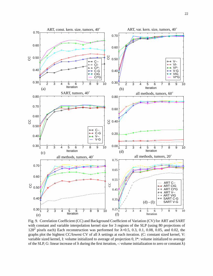
Fig. 9 shows a number of plots illustrating CC and CV for various reconstruction methods andparameter settings. Fig. 10 shows reconstructed SLP slice images after 3 iterations. The number of3 iterations was chosen because the plots indicate that after this number of iterations both CC andCV have reached a level close to their final value. In both Fig. 9 and Fig. 10 the following termi-nology is used. Each parameter combination is described by a 3 digit code. The first digit codes thesize of the interpolation kernel (C for constant, V for variable, depth-dependent). The second digitcodes the volume initialization method (- for zero, I for projection average, I* for SLP average).Lastly, the third digit codes the function at whichλ is varied during the first iteration (- for no vari-ation, G for linear increase). Reconstructions were obtained for each combination of parameter set-tings over the length of 10 iterations for all six settings ofλ. In order to keep the amount ofpresented data manageable, we do not plot the effect ofλ in Fig. 9. Instead, at every iteration andparameter combination we pick the lowest CV or highest CC, respectively, that was obtained in theset of sixλ-dependent reconstructions. As the idealλ is somewhat object-dependent anyway [17],this does not represent a serious trade-off. During the course of our experiments, we found that forART and the SLP theλ that produces good reconstructions within four iterations is somewherearound 0.08, for SART thisλ setting is around 0.3.

Fig. 9a-c shows the CC for the SLP tumors at a cone angle of 40˚ for the three main correctionmethods used: ART using the constant interpolation kernel, ART using the variable-size interpola-tion kernel, and SART using both kernels. In Fig. 9a we see that the reconstructions for G arealways better than the respective ones without G. Since it is not any costlier to do G, the followingplots will always use G. In Fig. 9b we see that reconstruction results with VIG are similar to the

21

ones with VI*G. Since VI*G is not realistic anyway, we will use only VIG for the remaining dis-cussion. In the same figure we also observe that V-G, VI- and VI*- yield only marginally worseresults than VIG, thus we will eliminate these settings from further plots. Finally, in Fig. 9c, we seethat SART C-G is either similar or always better than SART C--, and the same is true for SART V-G and SART V--. Thus we will be using only SART C-G and SART V-G. Also, preceding experi-ments revealed that SART is not dependent on the initial state of the volume. This is largely due tothe circumstance that SART corrects the volume on an image basis, which provides a good initial-ization after the first image was spread onto the volume.

The following plots (Fig. 9d-l) illustrate the effects of the settings of the remaining parameters onCC and CV. (Please use the legends inserted into Fig. 9f and i). In Fig. 9d, g, and j, we observe thatwhen using the constant sized interpolation kernel for ART, CC and CV for reconstructions at a 60˚cone angle improve significantly as volume initialization is made more accurate. This can also beseen in the reconstructed images shown in the first column of Fig. 10. If the volume is initializedto zero, the small SLP tumors (and other portions of the image) are completely obliterated by alias-ing artifacts (ART C--). The artifacts are reduced somewhat if the volume is initialized to the aver-age value of one of the projection images (ART CIG). The artifacts are reduced further, but stillwell noticeable, if the volume is initialized to the average value of the SLP brain matter (ARTCI*G). It is apparent that volume initialization alone cannot remove all artifacts. However, thereconstructions obtained with the variable sized interpolation kernel in conjunction with ART andthe ones obtained with SART are all artifact-free. The plots support these observation with onlySART and the ART V-methods having good CC and low CV. The plots also indicate that recon-struction quality increases when SART is used with a V-kernel instead of a C-kernel, however, theimprovements are not large. At the same token, reconstruction quality also improves when theART-V methods are used in conjunction with volume initialization and gradually increasing relax-ation coefficient, but the rate of improvement is at a much smaller scale than in the ART-C case.

From the images in the second column in Fig. 10 we observe that for a cone angle of 40˚ consid-erable artifacts around the tumors still remain for ART C-- and ART CIG. Again notice theimprovements with more accurate volume initialization. For ART CI*G, the artifacts are moreattenuated but are still visible (however, note again that ART CI*G may not always be realizable).On the other hand, with ART VIG and SART C-G, the artifacts are completely eliminated. Theplots of Fig. 9e, h, and k support these observations: the CCs are consistently higher, especially forsmall object detail like the SLP tumors, and the CVs are consistently lower with the ART V-meth-ods and SART than for the ART C-methods (with ART CI*G being closest to ART V and SART).

The plots of Fig. 9f, i, and l indicate that for a smaller cone angle of 20˚ the differences betweenthe methods are not as pronounced as for the larger cone angles, as long as one initializes the vol-ume at least with the average projection image value. The circumstance that ART VIG and SARTmaintain a marginally better CC for the SLP tumors in a quantitative sense could be relevant forautomated volume analysis and feature detection. However, in a visual inspection the differencesare hardly noticeable, as indicated in the reconstruction images in the third column of Fig. 10.

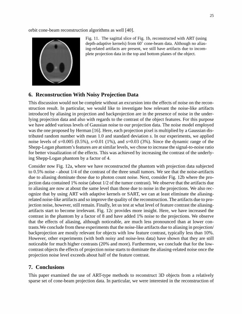
Finally, in Fig. 11 we show the sagittal cut of Fig. 1b, reconstructed with the new variant of ARTfrom 60˚ cone-angle projection data. We notice that although no aliasing artifacts due to the cone-beam projection/backprojection are present, we still have inaccuracies in the planes at the top andbottom of the phantom. These inaccuracies are due to the incompleteness of the projection dataobtained from the circular source orbit and have been observed in other single-source, circular-

22

Iteration

1 2 3 4 5 6 7 8 9 10Iteration

0.30

0.40

0.50

0.60

0.70

0.80

C-- C-G V-- V-G

Fig. 9. Correlation Coefficient (CC) and Background Coefficient of Variation (CV) for ART and SARTwith constant and variable interpolation kernel size for 3 regions of the SLP (using 80 projections of1282 pixels each) Each reconstruction was performed forλ=0.5, 0.3, 0.1, 0.08, 0.05, and 0.02, thegraphs plot the hightest CC/lowest CV of allλ settings at each iteration. (C: constant sized kernel, V:variable sized kernel, I: volume initialized to average of projection 0, I*: volume initialized to averageof the SLP, G: linear increase ofλ during the first iteration, -: volume initialization to zero or constantλ)

(c)

ART, const. kern. size, tumors, 40˚

SART, tumors, 40˚(a) (b)

1 2 3 4 5 6 7 8 9 100.30

0.40

0.50

0.60

V-- VI- VI*- V-G VIG VI*G

0.70C

CC

C

CC

1 2 3 4 5 6 7 8 9 10Iteration

0.30

0.40

0.50

0.60

0.70

ART, var. kern. size, tumors, 40˚

(d) - (l):

1 2 3 4 5 6 7 8 9 10Iteration

0.00

0.20

0.40

0.60

0.80

CC

all methods, tumors, 60˚

all methods, tumors, 40˚

1 2 3 4 5 6 7 8 9 10Iteration

0.30

0.40

0.50

0.60

0.70

CC

(e)

ART C-- ART CIG ART CI*G ART V-- ART VIG SART C-G SART V-G

all methods, tumors, 20˚

1 2 3 4 5 6 7 8 9 10Iteration

0.25

0.35

0.45

0.55

0.65

0.75

CC

(f)

(d)

C-- CI- CI*- C-G CIG CI*G

23

1 2 3 4 5 6 7 8 9 100.0

5.0

10.0

15.0

CV

(10

-3)

Iteration

Iteration Iteration

Fig. 9 (cont’d). CC and CV for ART and SART with constant and variable interpolation kernel size forthree regions of the 3D Shepp-Logan phantom. (C: constant sized kernel, V: variable sized kernel, I:volume initialized to average of projection 0, I*: volume initialized to average of Shepp-Logan brain,G: linear increase ofλ during the first iteration, -: volume initialization to 0 or constantλ)

(j)

(l)(k)1 2 3 4 5 6 7 8 9 100.0

1.0

2.0

3.0

4.0

5.0

1 2 3 4 5 6 7 8 9 100.0

0.5

1.0

1.5

2.0

2.5

3.0all methods, noise, 20˚all methods, noise, 40˚

all methods, noise, 60˚

Iteration(i)

Fig. 10. (next page): Slice of Fig. 1a reconstructed with various methods and cone angles

CV

(10

-3)

CV

(10

-3)

all methods, full head, 60˚

1 2 3 4 5 6 7 8 9 10Iteration

0.30

0.40

0.50

0.60

0.70

0.80

CC

(g)

all methods, full head, 40˚

1 2 3 4 5 6 7 8 9 10Iteration

0.60

0.70

0.80

0.90

CC

(h)

ART C-- ART CIG ART CI*G ART V-- ART VIG SART C-G SART V-G

all methods, full head, 20˚

(d) - (l):

CC

1 2 3 4 5 6 7 8 9 100.60

0.70

0.80

0.90

24

60̊ cone angle 40̊ cone angle 20̊ cone angle

ART C--

ART CIG

ART CI*G

ART VIG

SART C-G

Fig. 10

25

orbit cone-beam reconstruction algorithms as well [40].

6. Reconstruction With Noisy Projection DataThis discussion would not be complete without an excursion into the effects of noise on the recon-struction result. In particular, we would like to investigate how relevant the noise-like artifactsintroduced by aliasing in projection and backprojection are in the presence of noise in the under-lying projection data and also with regards to the contrast of the object features. For this purposewe have added various levels of Gaussian noise to our projection data. The noise model employedwas the one proposed by Herman [16]. Here, each projection pixel is multiplied by a Gaussian dis-tributed random number with mean 1.0 and standard deviations. In our experiments, we appliednoise levels ofs=0.005 (0.5%),s=0.01 (1%), ands=0.03 (3%). Since the dynamic range of theShepp-Logan phantom’s features are at similar levels, we chose to increase the signal-to-noise ratiofor better visualization of the effects. This was achieved by increasing the contrast of the underly-ing Shepp-Logan phantom by a factor of 4.

Consider now Fig. 12a, where we have reconstructed the phantom with projection data subjectedto 0.5% noise - about 1/4 of the contrast of the three small tumors. We see that the noise-artifactsdue to aliasing dominate those due to photon count noise. Next, consider Fig. 12b where the pro-jection data contained 1% noise (about 1/2 of the tumor contrast). We observe that the artifacts dueto aliasing are now at about the same level than those due to noise in the projections. We also rec-ognize that by using ART with adaptive kernels or SART, we can at least eliminate the aliasing-related noise-like artifacts and so improve the quality of the reconstruction. The artifacts due to pro-jection noise, however, still remain. Finally, let us test at what level of feature contrast the aliasing-artifacts start to become irrelevant. Fig. 12c provides more insight. Here, we have increased thecontrast in the phantom by a factor of 8 and have added 1% noise to the projections. We observethat the effects of aliasing, although noticeable, are much less pronounced than at lower con-trasts.We conclude from these experiments that the noise-like artifacts due to aliasing in projection/backprojection are mostly relevant for objects with low feature contrast, typically less than 10%.However, other experiments (with both noisy and noise-less data) have shown that they are stillnoticeable for much higher contrasts (20% and more). Furthermore, we conclude that for the low-contrast objects the effects of projection noise starts to dominate the aliasing-related noise once theprojection noise level exceeds about half of the feature contrast.

7. ConclusionsThis paper examined the use of ART-type methods to reconstruct 3D objects from a relativelysparse set of cone-beam projection data. In particular, we were interested in the reconstruction of

Fig. 11. The sagittal slice of Fig. 1b, reconstructed with ART (usingdepth-adaptive kernels) from 60˚ cone-beam data. Although no alias-ing-related artifacts are present, we still have artifacts due to incom-plete projection data in the top and bottom planes of the object.

26

low-contrast objects, which puts a high demand on the accuracy of the reconstruction algorithm.In the past, ART has seen frequent use for the cone-beam reconstruction of high-contrast objects,e.g. in computed angiography, however, the low-contrast case has not received much attention untilnow. One purpose of this paper was to present ART as an attractive alternative to the various FBP-type approaches that are mainly used in today’s general cone-beam reconstruction research. In par-ticular, it is the limited projection case where we see ART’s greatest potential. Even though ARTis iterative in nature, which was often equated with slowness of computation, our research indicatesthat really only three iterations are necessary to render a reconstruction result close to the optimum(given proper parameter settings). We found that ART’s present mechanism of computing theweight coefficients was insufficient for cone angles greater than 20˚ in that it lead to strong aliasingartifacts in the reconstructed object. We showed examples where small object detail was com-pletely obliterated by these aliasing artifacts. Even though these artifacts may have never been

(a)

(b)

(c)

Fig. 12. Reconstructions with noisy data and different levels of phantom contrasts: (a) 0.5% of noiseand 4 times the original contrast, (b) 1% of noise and 4 times the original contrast, (c) 1% of noise and8 times the original contrast. (2 iterations, all other parameters like Fig. 10.)

ART/ no adaptive filter ART/ adaptive filter SART

27

noticeable in high-contrast reconstructions, they become very visible in the low-contrast case. Toeliminate these artifacts, the new concept of depth-dependent interpolation kernels was introduced.By using these kernels we obtain cone-beam reconstructions free of cone-beam related aliasingartifacts. In this respect, it may be worthwhile to investigate if these kind of kernels are also usefulfor wide-angle cone-beam FBP reconstructions. On the other hand, apart from the ART correctionscheme, we also investigated the use of SART as an alternative correction algorithm. We found thatSART, being a projection-based correction procedure, is also very suitable to prevent the aliasingartifacts of traditional ART.

We then investigated the impact of volume initialization and the setting of the relaxation coefficientfor the various methods developed. Our results indicate that for cone angles of 60˚, as is often usedfor micro-tomography, strong aliasing artifacts prevail even with optimal volume initialization.These artifacts can only be eliminated when ART is used in conjunction with the depth-dependentkernel or by using SART. The same, though in a less dramatic way, is also true for cone angles of40˚, which are common-place in many clinical applications. For cone angles of 20˚ the aliasingeffects are not visible with either method, but can still be measured numerically.

Our research suggests that SART conceptually represents a better correction scheme than the tra-ditional ART approach, as it produces artifact-free reconstructions for all cone angles without theneed for depth-dependent interpolation kernel sizes. However, SART’s drawback is that it is noteasily accelerated. As other research [27] has indicated, ART is considerably easier to speed upthan SART, and runtime ratiosTSART/TART of approximately 1.5 have been observed. However, byusing elaborate methods for SART this ratio can be brought down to 1.15.

It should be mentioned that the ART methods outlined in this paper for cubic grids also fully extendto the dodecahedral grids that were proposed in [24]. These grids were shown to reduce the numberof voxels to be processed by about 30%.

We have demonstrated that our new variant of ART (and also SART) removes cone-beam relatedaliasing artifacts even when the projections are noisy. All that remains in the reconstructions arethe noise-related artifacts. Although it has often been said that ART performs poorly in the pres-ence of noise, Herman’s variants of ART, termed ART2 [15] and ART3 [16], were demonstratedto render superior results, at least when the projections were sparse. Since these algorithms weremostly studied in the early days of ART, with rather inaccurate projection methods, it would beinteresting to see how they perform with modern projection “technology”. Present research isunderway to investigate these pioneering algorithms, in addition to new variants.

Finally, in this paper we have restricted our reconstruction domain to an isolated spherical region,such as the human head. Of course, this is not always possible, for instance when imaging extendedobject such as the human torso. In this case, the circumstance that cone-beam rays at large angleswith respect to the mid-plane traverse object regions that are not part of the reconstructed objectregion is likely to have an adverse affect on the reconstruction result. This problem is generallycalled the “teepee effect” and is shown in Fig. 13a. We can prevent the teepee effect by using non-circular source paths (see e.g. [40]) or twin-cone source arrangements [21][36]. In the latter solu-tion, two cone-beam sources rotate on non-coplanar, coaxial, congruent, circular orbits around thepatient and the reconstruction algorithm only utilizes rays due to adjacent half-cones of these twopoint sources (see Fig. 13b). The distribution of rays in the cylindrical twin-cone region of interestis nearly homogeneous. Note that larger reconstruction regions will require larger cone-angles and

28

henceforth depth-adaptive interpolation kernels. At the same time, non-circular orbits and twin-cone arrangements will also improve the completeness of the projection data when the object doesfit into a sperical reconstruction region. (See e.g. Wang [40] for a comprehensive study). By usingthese trajectories we can reduce the remaining artifacts in the object planes further off the midplane(as shown in Fig. 11). Future work is planned to investigate the performance of the here presentedconcepts in conjunction with the twin-cone arrangement and other more advanced source trajecto-ries.

Appendix 1 - Accurate ray grid sampling rate

In Section 3 we used the approximate ray grid sampling rateωr. Consider Fig. 14 where we showone of several ways to estimate the accurate ray grid sampling rate at a volume grid positionwith z=zs andy=iTr. Here, is the index of the projection pixel andTr is the distance betweenthe points of intersection of the lines that go from the source to the pixel boundaries with the vol-ume slice plane atz=zs. The method uses the perpendicular distance between these two pixelbounding lines to compute for the ray of pixeli (see Fig. 14):

(26)

A plot of the rayfront for which is shown in Fig. 15.

reconstruction region

unaccountedlong objectray path

source source 1

source 2

reconstruction region

Fig. 13. (a) Single cone geometry: rays at large angles with respect to the mid-plane traverse regionsoutside the reconstruction sphere, (b) twin-cone geometry: a nearly homogenous ray density is achievedin the cylindrical volume section that is traversed by the two adjacent twin half-cones [21][36].

(a) (b)

ωrˆ

i ℵ∈

Trˆ

ω̂r 1 Trˆ⁄=

Trˆ Tr ϕcos

zs

zc----Tg ϕcos=≈

zs

zc----Tg

zc

iTg⟨ ⟩2zc

2+

-------------------------------⋅zsTg

iTg⟨ ⟩2zc

2+

-------------------------------= =

Trˆ Tg 1= =

29

Appendix 2 - Errors when approximating the ray grid sampling rate

The relative errorestretchwhen usingTr instead of for stretching the kernel functions is given by:

(27)

This error is plotted in Fig. 16.

zc zs z

y=iTg

ϕTr

Trˆ

Tg

Fig. 14. Computing the perpendicular ray distanceto estimate the accurate ray grid sampling rate. The dashed line is the ray that traverses from

the source through the center of projection pixeli=2. The lines (shown in solid) that connect thepixel boundaries with the source intersect the vol-ume slice atz=zs. The distance between these inter-sections isTr, and1/Tr was used in Section 3 as theapproximate ray grid sampling rate.Tg is the periodof the volume grid andzc is the slice in whichTr=Tg. Finally, is given by the perpendiculardistance of the two pixel boundary rays atz=zs.

Trˆ

ωrˆ

Trˆ

0Tg

2Tg

3Tg

-Tg

p2

p0

p1

p-1

projection plane

Fig. 15. Shape of the rayfront with constant .Here the case of is shown. In the regionson the left side of the curve the ray grid samplingrate is higher than the sampling rate of the volumegrid, while in the regions on the right of the curvethe ray grid sampling rate is lower than the volumegrid sampling rate.

ωrˆ

ωrˆ 1.0=

z

iTg

Trˆ

estretch Tr Trˆ⁄

zs

zc----Tg⟨ ⟩

zsTg

iTg⟨ ⟩2zc

2+

-------------------------------⟨ ⟩⁄iTg⟨ ⟩2

zc2

+

zc-------------------------------= = =

Fig. 16. The relative errorestretch when usingTrinstead of for stretching the kernel functions.We see that further away from the cone center thekernel is stretched too much if the curved ray frontis approximated by a planar rayfront to estimateωr.This means that the grid signal is overly smoothedwhen sampled. The maximum error of 15% occursat the cone boundary. This means that the kernel isstretched 15% more than necessary.

Trˆ

iTg

e str

etc

h

30

Acknowledgments

This work was performed with the generous support of General Electric under CCH grant #950925and OSU grant #732025. We would also like to thank the anonymous reviewers for their carefulreading of the manuscripts and their suggestions.

References

[1] M.D. Altschuler, G.T. Herman, and A. Lent, “Fully three-dimensional image reconstruction from cone-beamsources,”Proc. Conf. Pattern Recognition and Image Processing, IEEE Computer Society, pp. 194-199, 1978.

[2] M.D. Altschuler and G.T. Herman, “Fully three-dimensional image reconstruction using series expansion meth-ods,”A Review of Information Processing in Medical Imaging, A.B. Brill et. al. (Eds.), Oak Ridge National Lab,pp. 125-142, 1977.

[3] M.D. Altschuler, Y. Censor, P.P.B. Eggermont, G.T. Herman, Y.H. Kuo, R.M. Lewitt, M. McKay, H.K. Tuy,J.K. Udupa, and M.M. Yau, “Demonstration of a software package for the reconstruction of a dynamicallychanging structure of the human heart from cone-beam X-ray projections,”J. Med. Syst., vol. 4, no. 2, pp. 289-304, 1980.

[4] A. H. Andersen, “Algebraic Reconstruction in CT from Limited Views,”IEEE Trans. Med. Img., vol. 8, no.1,pp. 50-55, 1989.

[5] A.H. Andersen and A.C. Kak, “Simultaneous Algebraic Reconstruction Technique (SART): a superior imple-mentation of the ART algorithm,”Ultrason. Img., vol. 6, pp. 81-94, 1984.

[6] C. Axelson, “Direct Fourier methods in 3D reconstruction from cone-beam data,”Thesis, Linkoping University,1994.

[7] R.N. Bracewell,The Fourier Transform and Its Applications, 2nd ed., McGraw-Hill, Inc., 1986.

[8] T.F. Budinger and G.T. Gullberg, “Three-dimensional reconstruction in nuclear medicine imaging,”IEEETrans. Nucl. Sci., vol. 21, pp. 2-19, June 1974.

[9] J.G. Colsher, “Iterative three-dimensional image reconstruction from tomographic projections,”ComputerGraphics and Image Processing, no. 6, pp. 513-537, 1977.

[10] C. R. Crawford and K. F. King, “Computed tomography scanning with simultaneous patient translation,”Med-ical Physics, vol. 17, pp. 967-982, 1990.

[11] R. Gordon, R. Bender, and G.T. Herman, “Algebraic reconstruction techniques (ART) for three-dimensionalelectron microscopy and X-ray photography,”J. Theoretical Biology, vol. 29, pp. 471-481, 1970.

[12] H. Guan and R. Gordon, “Computed tomography using algebraic reconstruction techniques (ARTs) with dif-ferent projection access schemes: a comparison study under practical situations,”Phys. Med. Biol., no. 41, pp.1727-1743, 1996.

[13] K.M. Hanson and G.W. Wecksung, “Local basis-function approach to computed tomography,”Applied Optics,Vol. 24, No. 23, 1985.

[14] G.T. Herman,Image Reconstruction from Projections: The Fundamentals of Computerized Tomography. NewYork: Academic Press, 1980.

[15] G.T. Herman, A. Lent, and S.W. Rowland, “ART: Mathematics and applications. A report on the mathematicalfoundations and on the applicability to real data of the Algebraic Reconstruction Technique,”J. Theor. Biol.,vol. 42, pp. 1-32, 1973.

[16] G.T. Herman, “A relaxation method for reconstructing objects from noisy X-rays,”Mathematical Program-ming, vol. 8, pp. 1-19, 1975.

[17] G.T. Herman and L.B. Meyer, “Algebraic reconstruction can be made computationally efficient,”IEEE Trans.Med. Img., vol. 12, no. 3, pp. 600-609, 1993.

[18] A. Kaufman, Ed., Volume Visualization, IEEE Press 1991.

[19] S. Kaczmarz, “Angenäherte Auflösung von Systemen linearer Gleichungen,”Bull. Int. Acad. Pol. Sci. Lett., A,vol. 35, pp. 335-357, 1937.

[20] A.C. Kak and M. Slaney,Principles of Computerized Tomographic Imaging. IEEE Press, 1988.

[21] G. Kowalski, “Multislice reconstruction from twin-cone beam scanning,”IEEE Trans. Nucl. Sci., vol. 26, no.

31

2, pp. 2895-2903, 1979.

[22] R.M. Lewitt, “Alternatives to voxels for image representation in iterative reconstruction algorithms,”Phys.Med. Biol., vol. 37, no. 3, pp. 705-715, 1992.

[23] S. Matej and R.M. Lewitt, “Practical considerations for 3-D image reconstruction using spherically symmetricvolume elements,” IEEE Trans. Med. Img., vol. 15, no. 1, pp. 68-78, 1996.

[24] S. Matej and R.M. Lewitt, “Efficient 3D grids for image reconstruction using spherically-symmetric volumeelements,”IEEE Trans. on Nucl. Sci., vol. 42, no 4, pp 1361-1370, 1995.

[25] S. Matej, G.T. Herman, T.K. Narayan, S.S. Furuie, R.M. Lewitt, and P.E. Kinahan, “Evaluation of task-orientedperformance of several fully 3D PET reconstruction algorithms,”Phys. Med. Biol, Vol. 39, pp. 355-367, 1994.

[26] E.J. Mazur and R. Gordon, “Interpolative algebraic reconstruction techniques without beam partioning for com-puted tomography,”Med. & Biol. Eng. & Comput., vol. 33, pp. 82-86, 1995.

[27] K. Mueller, R. Yagel and J.J. Wheller “Fast implementations of the Algebraic Reconstruction Technique(ART),” to appear inIEEE Transaction on Medical Imaging, September 1999.

[28] K. Mueller, R. Yagel, and J.F. Cornhill, “The weighted distance scheme: a globally optimizing projection order-ing method for the Algebraic Reconstruction Technique (ART),”IEEE Transactions on Medical Imaging, vol.16, no. 2, pp. 223-230, April 1997.

[29] F. Natterer,The Mathematics of Computerized Tomography, Wiley, 1986.

[30] R. Ning and S.J. Rooker, “Image intensifier-based volume angiography imaging system: work in progress,”Proc. SPIE, vol. 1896, Medical Imaging 1993: Physics of Medical Imaging, pp. 145-155, 1993.

[31] P. Rizo, P. Grangeat, P. Sire, P. Lemasson, and P. Melennec, “Comparison of three-dimensional x-ray cone-beam reconstruction algorithms with circular source trajectories,”J. Opt. Soc. Am. A, vol. 8, no. 10, pp.1639-1648.

[32] R.A. Robb, “The dynamic spatial reconstructor: an X-ray video-fluoroscopic CT scanner for dynamic volumeimaging of moving organs,”IEEE Trans. Med. Img., vol. 1, no. 1, pp. 22-33, 1982.

[33] D. Ros, C. Falcon, I Juvells, and J. Pavia, “The influence of a relaxation parameter on SPECT iterative recon-struction algorithms,”Phys. Med. Biol., no. 41, pp. 925-937, 1996.

[34] D. Saint-Felix, Y. Trousset, C. Picard, C. Ponchut, R. Romeas, A. Rougee, “In vivo evaluation of a new systemfor 3D computerized angiography,”Phys. Med. Biol, Vol. 39, pp. 583-595, 1994.

[35] L.A. Shepp and B.F. Logan, “The Fourier reconstruction of a head section,”IEEE Trans. Nucl. Sci., vol. NS-21, pp. 21-43, 1974.

[36] M. Schlindwein, “Iterative three-dimensional reconstruction from twin-cone beam projections,”IEEE Trans.Nucl. Sci., vol. 25, no. 5, pp. 1135-1143, 1978.

[37] B. Smith, “Cone-beam tomography: recent advances and a tutorial review,”Optical Engineering, vol. 29, no.5, pp. 524-534, 1990.

[38] J.E. Swan, K. Mueller, T. Moeller, N. Shareef, R. Crawfis, and R. Yagel, “An anti-aliasing technique for splat-ting,” Proceedings Visualization’97, pp. 197-204, 1997.

[39] K.C. Tam, S. Samarasekera, and F. Sauer, “ Region-of-interest cone-beam CT with a spiral scan,”Proc. 1998SPIE Medical Imaging Conference, SPIE vol. 3336, 1998.

[40] G. Wang, T. Lin, P. Cheng, and D.M. Shinozaki, “A general cone-beam reconstruction algorithm,”IEEE.Trans. Med. Imag., vol. 12, no. 3, pp. 486-496, 1993.

[41] L. Westover, “Footprint evaluation for volume rendering,”Computer Graphics (SIGGRAPH), vol. 24, no. 4,pp. 367-376, 1990.