antineutrino oscillations and a search for nsi with...
TRANSCRIPT
ANTINEUTRINO OSCILLATIONS AND A SEARCH
FOR NON-STANDARD INTERACTIONS WITH
THE MINOS EXPERIMENT
by
Zeynep Isvan
B.S., Physics, Bosphorus University, Istanbul, Turkey, 2005
M.Sc., Physics, University of Pittsburgh, 2006
Submitted to the Graduate Faculty of
the Kenneth P. Dietrich School of Arts and Sciences
in partial fulfillment
of the requirements for the degree of
Doctor of Philosophy
University of Pittsburgh
2012
UNIVERSITY OF PITTSBURGH
DEPARTMENT OF PHYSICS AND ASTRONOMY
This dissertation was presented
by
Zeynep Isvan
It was defended on
January 6th 2012
and approved by
Dr. Donna Naples, University of Pittsburgh, Department of Physics and Astronomy
Dr. Ayres Freitas, University of Pittsburgh, Department of Physics and Astronomy
Dr. Vittorio Paolone, University of Pittsburgh, Department of Physics and Astronomy
Dr. Lincoln Wolfenstein, Carnegie Mellon University, Department of Physics
Dr. Michael Wood-Vasey, University of Pittsburgh, Department of Physics and Astronomy
Dissertation Director: Dr. Donna Naples, University of Pittsburgh, Department of Physics
and Astronomy
ii
Copyright c© by Zeynep Isvan
2012
iii

ANTINEUTRINO OSCILLATIONS AND A SEARCH FOR
NON-STANDARD INTERACTIONS WITH THE MINOS EXPERIMENT
Zeynep Isvan, PhD
University of Pittsburgh, 2012
MINOS searches for neutrino oscillations using the disappearance of muon neutrinos from
the NuMI beam at Fermilab between two detectors. The Near Detector, located near the
source, measures the beam composition before flavor change occurs. The energy spectrum
is measured again at the Far Detector after neutrinos travel a distance. The mixing angle
and mass splitting between the second and third mass states are extracted from the energy
dependent difference between the spectra at the two detectors. NuMI is able to produce
an antineutrino-enhanced beam as well as a neutrino-enhanced beam. Collecting data in
antineutrino-mode allows the direct measurement of antineutrino oscillation parameters.
From the analysis of the antineutrino mode data we measure |∆m2atm| = 2.62+0.31
−0.28× 10⁻³eV2
and sin2(2θ)23 = 0.95+0.10−0.11, which is the most precise measurement of antineutrino oscillation
parameters to date.
A difference between neutrino and antineutrino oscillation parameters may indicate new
physics involving interactions that are not part of the Standard Model, called non-standard
interactions, that alter the apparent disappearance probability. Collecting data in neutrino
and antineutrino mode independently allows a direct search for non-standard interactions.
In this dissertation non-standard interactions are constrained by a combined analysis of
neutrino and antineutrino datasets and no evidence of such interactions is found.
iv
TABLE OF CONTENTS
PREFACE . . . . . . . . . . . . . . . . . . . . . . . . . . . . . . . . . . . . . . . . . xv
1.0 INTRODUCTION . . . . . . . . . . . . . . . . . . . . . . . . . . . . . . . . . 1
1.1 History of Neutrinos . . . . . . . . . . . . . . . . . . . . . . . . . . . . . . 2
1.2 The Standard Model . . . . . . . . . . . . . . . . . . . . . . . . . . . . . . 3
1.2.1 The Weak Interaction . . . . . . . . . . . . . . . . . . . . . . . . . . 5
1.2.1.1 Charged-current (CC) neutrino-electron scattering . . . . . 6
1.2.1.2 Charged-current neutrino-quark scattering . . . . . . . . . . 7
1.2.1.3 Neutral current (NC) neutrino-quark scattering . . . . . . . 10
1.2.2 The Electroweak Interaction . . . . . . . . . . . . . . . . . . . . . . 12
1.2.2.1 Neutral current neutrino-electron scattering . . . . . . . . . 14
1.3 Neutrino Mixing and Mass . . . . . . . . . . . . . . . . . . . . . . . . . . . 15
1.3.1 Three Flavor Case . . . . . . . . . . . . . . . . . . . . . . . . . . . 17
1.3.2 Two Flavor Case . . . . . . . . . . . . . . . . . . . . . . . . . . . . 18
1.4 Neutrino Oscillation and CPT Symmetry . . . . . . . . . . . . . . . . . . . 19
1.5 Neutrino Oscillations in Matter . . . . . . . . . . . . . . . . . . . . . . . . 20
1.6 Non-Standard Matter Interactions . . . . . . . . . . . . . . . . . . . . . . . 22
1.7 Status of Measurements and Remarks . . . . . . . . . . . . . . . . . . . . . 25
1.7.1 Non-standard Interactions . . . . . . . . . . . . . . . . . . . . . . . 28
2.0 THE MINOS BEAM AND DETECTORS . . . . . . . . . . . . . . . . . . 31
2.1 The NuMI Beam . . . . . . . . . . . . . . . . . . . . . . . . . . . . . . . . 32
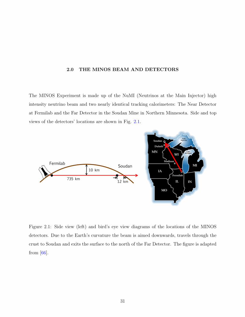
2.2 The MINOS Detectors . . . . . . . . . . . . . . . . . . . . . . . . . . . . . 38
2.2.1 Near Detector . . . . . . . . . . . . . . . . . . . . . . . . . . . . . . 40
v
2.2.2 Far Detector . . . . . . . . . . . . . . . . . . . . . . . . . . . . . . . 41
2.3 Scintillator . . . . . . . . . . . . . . . . . . . . . . . . . . . . . . . . . . . . 42
2.4 Photomultiplier Tubes . . . . . . . . . . . . . . . . . . . . . . . . . . . . . 43
2.5 The Magnetic Field . . . . . . . . . . . . . . . . . . . . . . . . . . . . . . . 44
2.6 Electronics and Data Acquisition . . . . . . . . . . . . . . . . . . . . . . . 46
2.6.1 Near Detector Front-End Electronics . . . . . . . . . . . . . . . . . 46
2.6.2 Far Detector Front-End Electronics . . . . . . . . . . . . . . . . . . 51
2.6.3 Data Acquisition . . . . . . . . . . . . . . . . . . . . . . . . . . . . 52
2.7 Calibration Detector . . . . . . . . . . . . . . . . . . . . . . . . . . . . . . 53
2.8 Near and Far Detector Differences . . . . . . . . . . . . . . . . . . . . . . . 56
3.0 EVENT RECONSTRUCTION, CALIBRATION AND MONTE CARLO
SIMULATION . . . . . . . . . . . . . . . . . . . . . . . . . . . . . . . . . . . 57
3.1 Reconstruction . . . . . . . . . . . . . . . . . . . . . . . . . . . . . . . . . 58
3.1.1 Slice Formation . . . . . . . . . . . . . . . . . . . . . . . . . . . . . 58
3.1.2 Track Reconstruction . . . . . . . . . . . . . . . . . . . . . . . . . . 58
3.1.3 Cluster Formation and Shower Reconstruction . . . . . . . . . . . . 60
3.1.4 Event Formation . . . . . . . . . . . . . . . . . . . . . . . . . . . . 62
3.2 Calibration . . . . . . . . . . . . . . . . . . . . . . . . . . . . . . . . . . . 62
3.2.1 Calibration Procedure . . . . . . . . . . . . . . . . . . . . . . . . . 63
3.2.1.1 PMT and Electronics Drift DPMT(d, t) . . . . . . . . . . . 63
3.2.1.2 Linearity L(d, s,Qraw) . . . . . . . . . . . . . . . . . . . . 64
3.2.1.3 Scintillator Drift Correction Dscint(d, t) . . . . . . . . . . . 64
3.2.1.4 Strip-to-strip Calibration S(s, d, t) . . . . . . . . . . . . . 64
3.2.1.5 Attenuation A(d, s, x) . . . . . . . . . . . . . . . . . . . . 65
3.2.1.6 Inter-detector Calibration M(d) . . . . . . . . . . . . . . . 65
3.2.2 Absolute Energy Scale . . . . . . . . . . . . . . . . . . . . . . . . . 66
3.3 Monte Carlo Simulation . . . . . . . . . . . . . . . . . . . . . . . . . . . . 66
4.0 ANTINEUTRINO OSCILLATION ANALYSIS . . . . . . . . . . . . . . 68
4.1 Event Topologies . . . . . . . . . . . . . . . . . . . . . . . . . . . . . . . . 68
4.2 Event Selection . . . . . . . . . . . . . . . . . . . . . . . . . . . . . . . . . 70
vi
4.2.1 Pre-selection . . . . . . . . . . . . . . . . . . . . . . . . . . . . . . . 70
4.2.2 Far Detector Fiducial Volume . . . . . . . . . . . . . . . . . . . . . 70
4.2.3 Near Detector Fiducial Volume . . . . . . . . . . . . . . . . . . . . 71
4.2.4 Separation of charged-current and neutral-current events . . . . . . 72
4.3 Charge sign selection . . . . . . . . . . . . . . . . . . . . . . . . . . . . . . 77
4.4 Near Detector Track End Cut . . . . . . . . . . . . . . . . . . . . . . . . . 78
4.5 Beam Tuning . . . . . . . . . . . . . . . . . . . . . . . . . . . . . . . . . . 79
4.6 Near Detector Event Sample . . . . . . . . . . . . . . . . . . . . . . . . . . 83
4.7 Near to Far Extrapolation . . . . . . . . . . . . . . . . . . . . . . . . . . . 87
4.8 Systematic Uncertainties . . . . . . . . . . . . . . . . . . . . . . . . . . . . 91
4.8.1 Muon energy scale . . . . . . . . . . . . . . . . . . . . . . . . . . . 91
4.8.2 Hadronic energy scale . . . . . . . . . . . . . . . . . . . . . . . . . . 92
4.8.3 Relative normalization . . . . . . . . . . . . . . . . . . . . . . . . . 93
4.8.4 Backgrounds . . . . . . . . . . . . . . . . . . . . . . . . . . . . . . . 94
4.8.5 Cross section uncertainties . . . . . . . . . . . . . . . . . . . . . . . 95
4.8.6 Smaller sources of systematic uncertainties . . . . . . . . . . . . . . 95
4.9 Far Detector Selection . . . . . . . . . . . . . . . . . . . . . . . . . . . . . 96
4.10 Fitting the Data . . . . . . . . . . . . . . . . . . . . . . . . . . . . . . . . 101
4.10.1 Evaluation of Oscillation Parameter Uncertainties . . . . . . . . . . 105
5.0 NON-STANDARD INTERACTIONS ANALYSIS . . . . . . . . . . . . . 110
5.1 The Neutrino Dataset . . . . . . . . . . . . . . . . . . . . . . . . . . . . . 110
5.1.1 Separation of charged-current and neutral-current events . . . . . . 111
5.1.2 Near Detector Sample . . . . . . . . . . . . . . . . . . . . . . . . . 113
5.1.3 Far Detector Sample . . . . . . . . . . . . . . . . . . . . . . . . . . 116
5.2 Antineutrino Selected Sample . . . . . . . . . . . . . . . . . . . . . . . . . 119
5.3 Near to Far Extrapolation . . . . . . . . . . . . . . . . . . . . . . . . . . . 120
5.4 Systematic uncertainties . . . . . . . . . . . . . . . . . . . . . . . . . . . . 120
5.5 Fitting the Data . . . . . . . . . . . . . . . . . . . . . . . . . . . . . . . . 121
5.5.1 Evaluation of NSI parameter Uncertainties . . . . . . . . . . . . . . 128
6.0 CONCLUSION AND OUTLOOK . . . . . . . . . . . . . . . . . . . . . . . 132
vii
6.1 Future Measurements and Experiments . . . . . . . . . . . . . . . . . . . . 134
BIBLIOGRAPHY . . . . . . . . . . . . . . . . . . . . . . . . . . . . . . . . . . . . 136
viii

LIST OF TABLES
1.1 Fundamental particles of the Standard Model . . . . . . . . . . . . . . . . . . 4
4.1 Contributions to the relative near/far normalization uncertainty . . . . . . . 94
4.2 Systematic uncertainties and their effect on the oscillation fit . . . . . . . . . 109
5.1 Systematic uncertainties included in the fit and their pulls . . . . . . . . . . 123
5.2 Systematic uncertainties and their effect on the NSI fit . . . . . . . . . . . . 129
ix

LIST OF FIGURES
1.1 Feynman diagrams of CC ν − e and ν − e interactions . . . . . . . . . . . . . 6
1.2 Feynman diagrams of CC ν − q and ν − q interactions . . . . . . . . . . . . . 7
1.3 Feynman diagram of NC ν − q scattering . . . . . . . . . . . . . . . . . . . . 10
1.4 Neutrino oscillation results from KamLAND . . . . . . . . . . . . . . . . . . 27
2.1 Side view and bird’s eye view diagrams of the locations of the MINOS detectors 31
2.2 The NuMI beamline . . . . . . . . . . . . . . . . . . . . . . . . . . . . . . . . 32
2.3 The NuMI target . . . . . . . . . . . . . . . . . . . . . . . . . . . . . . . . . 33
2.4 Upstream beamline geometry and focusing optics . . . . . . . . . . . . . . . . 35
2.5 Near Detector simulated energy spectra in FHC-mode . . . . . . . . . . . . . 36
2.6 Near Detector simulated energy spectra in RHC-mode . . . . . . . . . . . . . 36
2.7 NuMI beam configurations . . . . . . . . . . . . . . . . . . . . . . . . . . . . 37
2.8 MINOS detector planes . . . . . . . . . . . . . . . . . . . . . . . . . . . . . . 38
2.9 Near Detector planes . . . . . . . . . . . . . . . . . . . . . . . . . . . . . . . 39
2.10 Far Detector planes . . . . . . . . . . . . . . . . . . . . . . . . . . . . . . . . 39
2.11 Cross sectional view of a Near Detector plane . . . . . . . . . . . . . . . . . . 40
2.12 Cross sectional view of a MINOS scintillator strip . . . . . . . . . . . . . . . 42
2.13 The readout chain from WLS fibers to PMTs . . . . . . . . . . . . . . . . . . 43
2.14 Cross section of a Far Detector Coil . . . . . . . . . . . . . . . . . . . . . . . 45
2.15 Near and Far Detector magnetic field maps . . . . . . . . . . . . . . . . . . . 45
2.16 Block diagram of the QIE chip for the Near Detector . . . . . . . . . . . . . 47
2.17 Response of a Near Detector QIE chip . . . . . . . . . . . . . . . . . . . . . . 48
2.18 Block diagrams of a MENU and a MINDER module . . . . . . . . . . . . . . 49
x

2.19 Overview of the Near Detector front-end electronics . . . . . . . . . . . . . . 50
2.20 Overview of the Far Detector front-end electronics . . . . . . . . . . . . . . . 51
2.21 Components of the MINOS data acquisition system . . . . . . . . . . . . . . 52
2.22 A CalDet subsection of 12 planes . . . . . . . . . . . . . . . . . . . . . . . . 54
2.23 CalDet response to pions and electrons . . . . . . . . . . . . . . . . . . . . . 55
3.1 A Near Detector snarl . . . . . . . . . . . . . . . . . . . . . . . . . . . . . . . 59
4.1 Event topologies of CC and NC interactions in the MINOS detectors . . . . . 69
4.2 Far Detector fiducial volume . . . . . . . . . . . . . . . . . . . . . . . . . . . 71
4.3 Sketch demonstrating the kNN particle identification method . . . . . . . . . 73
4.4 Efficiency and purity distributions of two event selectors . . . . . . . . . . . . 74
4.5 Distributions of kNN input variables . . . . . . . . . . . . . . . . . . . . . . . 75
4.6 Distribution of CC/NC separation parameter . . . . . . . . . . . . . . . . . . 76
4.7 q/p distribution of Near Detector events . . . . . . . . . . . . . . . . . . . . . 77
4.8 End positions of ND events that fail the track fitter . . . . . . . . . . . . . . 78
4.9 The reconstructed antineutrino energy distribution at the Near Detector . . . 79
4.10 Data, tuned and untuned Monte Carlo Near Detector neutrino energy distri-
bution . . . . . . . . . . . . . . . . . . . . . . . . . . . . . . . . . . . . . . . 81
4.11 Data, tuned and untuned Monte Carlo Near Detector antineutrino energy
distribution . . . . . . . . . . . . . . . . . . . . . . . . . . . . . . . . . . . . 82
4.12 Efficiency and contamination of the Near Detector antineutrino selection . . . 83
4.13 Near Detector antineutrino energy and inelasticity distributions . . . . . . . . 84
4.14 Near Detector antineutrino event position distributions . . . . . . . . . . . . 85
4.15 Distributions of antineutrino selection cut variables . . . . . . . . . . . . . . 86
4.16 Acceptance of meson decay angles by the Near and Far Detectors . . . . . . . 87
4.17 FD flux over the ND flux before extrapolation . . . . . . . . . . . . . . . . . 88
4.18 Simulated true energy spectra at the Near and Far Detectors . . . . . . . . . 88
4.19 Flowchart of the beam matrix extrapolation method . . . . . . . . . . . . . . 89
4.20 Antineutrino beam matrix . . . . . . . . . . . . . . . . . . . . . . . . . . . . 91
4.21 Systematic uncertainty on the shower energy measurement . . . . . . . . . . 92
4.22 Efficiency and contamination of the Far Detector antineutrino selection . . . 97
xi
4.23 Far Detector antineutrino energy distributions . . . . . . . . . . . . . . . . . 98
4.24 Far Detector antineutrino transverse position distributions . . . . . . . . . . 98
4.25 Far Detector antineutrino position distributions . . . . . . . . . . . . . . . . 99
4.26 Far Detector antineutrino track and shower energy distributions . . . . . . . 100
4.27 Far Detector distribution of antineutrino angle with respect to the beam direction100
4.28 Feldman-Cousins surface corresponding to 90% coverage . . . . . . . . . . . . 102
4.29 Comparison of the Feldman-Cousins method to Gaussian statistics . . . . . . 103
4.30 Far Detector antineutrino data and prediction energy spectra . . . . . . . . . 104
4.31 The 68%, 90%, and 99% antineutrino oscillation contours . . . . . . . . . . . 105
4.32 Effect of systematic uncertainties on the best oscillation fit . . . . . . . . . . 106
4.33 The total systematic error band on the number of predicted νµ events . . . . 107
4.34 Comparison of systematic and statistical uncertainty . . . . . . . . . . . . . . 108
5.1 MINOS neutrino oscillation analysis allowed regions . . . . . . . . . . . . . . 111
5.2 Distribution of neutrino CC/NC separation variables . . . . . . . . . . . . . 112
5.3 Efficiency and contamination of the Near Detector neutrino selection . . . . . 113
5.4 Near Detector neutrino energy and inelasticity distributions . . . . . . . . . . 114
5.5 Near Detector neutrino event position distributions . . . . . . . . . . . . . . 115
5.6 Efficiency and contamination of the Far Detector neutrino selection . . . . . 116
5.7 Far Detector neutrino position distributions . . . . . . . . . . . . . . . . . . . 117
5.8 Far Detector neutrino energy distributions . . . . . . . . . . . . . . . . . . . 118
5.9 Far Detector distribution of neutrino angle with respect to the beam direction 118
5.10 Efficiency and contamination of the Near Detector antineutrino NSI selection 119
5.11 Systematic error bands from the four largest systematics . . . . . . . . . . . 122
5.12 Far Detector neutrino data and prediction energy spectra . . . . . . . . . . . 124
5.13 Far Detector antineutrino data and prediction energy spectra . . . . . . . . . 125
5.14 68% and 90% NSI contours . . . . . . . . . . . . . . . . . . . . . . . . . . . . 126
5.15 One dimensional ∆χ2 distributions of NSI parameters . . . . . . . . . . . . . 127
5.16 Effect of systematic uncertainties on the best NSI fit . . . . . . . . . . . . . . 130
5.17 Comparison of systematic and statistical uncertainties of the NSI analysis . . 131
6.1 90% C.L. contours for the published MINOS antineutrino oscillation result . 133
xii

6.2 The evolution of the 90% contours of antineutrino oscillation parameters with
increasing data . . . . . . . . . . . . . . . . . . . . . . . . . . . . . . . . . . . 134
xiii

This dissertation is dedicated to my grandfather Ahmet Vamık Isvan,
whose profound appreciation for and commitment to the scientific method inspires me,
and to my grandmother Cumhuriyet Reha Isvan,
who taught not only me but generations of young women and men to fulfill their dreams,
with infinite gratitude and love.
xiv

PREFACE
Thanks go first and foremost to my adviser Donna Naples, an exceptional mentor, who
provided all the support and guidance I needed while encouraging me to take charge and
become a self-reliant researcher. She always provided insight, perspective and the big picture
context.
I am indebted to my undergraduate advisor Levent Kurnaz and my professors Teoman
Turgut and Engin Arik for starting me on this journey. Peter Koehler helped me discover
and pursue my research field. Our graduate secretary Leyla Hirschfeld deserves much credit
for making the entire process manageable. I would also like to thank the Pitt neutrino group
for their collaboration.
This work would not be possible without all members of MINOS. I would particularly
like to thank the NuMuBar group and its conveners Justin Evans, Jeff Hartnell, Mike Kor-
dosky, Donna Naples and Alex Sousa. Tony Mann has pioneered the study of non-standard
interactions on MINOS and offered me careful feedback at every step of my analysis. Alex
Himmel deserves special thanks for his help over the years and for the documentation and
code he left behind. I would like to thank Chris Backhouse, who not only had answers to
all my statistics and programming questions but also the patience to explain them.
Young MINOS, my Village neighbors and the rest of the Fermilab gang, the GSA, Chivas,
Two Brothers and my oldest friend Elif were always there to keep me sane; thank you all.
Ulysses, thank you for making the hardest final stretch meaningful and memorable.
Finally, I would like to thank my family who have supported me throughout graduate
school, often financially. You have set the bar high and always been proud of me. I would
not be here without you.
xv

1.0 INTRODUCTION
The two topics addressed in this thesis are antineutrino oscillations and non-standard neutrino-
matter interactions, neither of which is described by the Standard Model (SM) of particle
physics. In the SM neutrinos (and antineutrinos) are massless. There is, however, evidence
that they change flavor upon traveling a distance, which is only possible in vacuum if at least
two of the three active neutrinos are massive. This phenomenon is called oscillation because
the probability of flavor change depends on the distance traveled (and neutrino energy) and
has an oscillatory shape. Neutrino oscillation experiments aim to probe the extensions to
the SM which include non-zero masses. We investigate this phenomenon for antineutrinos
and measure the parameters that govern their flavor change.
In neutrino oscillation experiments neutrinos travel through matter and are not propa-
gating in vacuum. This allows other flavor change mechanisms whereby neutrinos take part
in new physics interactions within and beyond the SM. While in theory such non-standard
interactions (NSI) will cause flavor change even for massless neutrinos, observed flavor change
effects are too large to be explained solely by NSI within their current limits. In this thesis
we treat NSI as a perturbation to the oscillation model and assume the two effects jointly
influence flavor change.
This chapter begins with a brief introduction to the history of neutrino physics and con-
tinues to discuss the SM, with an emphasis on weak interactions since neutrinos only interact
weakly. Neutrino mass and mixing is discussed next assuming matter effects are negligible
(i.e. vacuum oscillations). A discussion of standard matter effects, that is, effects from neu-
trino interactions described by the SM and the way these alter oscillations follows. Finally,
the phenomenology of the non-standard interactions considered in this thesis, namely, flavor
changing neutral current neutrino-matter interactions, is presented. The history and current
1

limits of neutrino oscillation and non-standard interactions are discussed in the last section.
Chapter 2 discusses the generation and key features of the NuMI beam, the design of
MINOS detectors and how these relate to the physics measurements. Chapter 3 details the
process of event reconstruction and calibration as well as Monte Carlo simulation, which is
key to understanding and interpreting the probabilistic processes of particle physics from
the limited data statistics. Chapters 4 and 5 present detailed accounts of the antineutrino
oscillation and non-standard interactions analyses, respectively, and report the findings.
Chapter 6 concludes and offers a future outlook.
1.1 HISTORY OF NEUTRINOS
Physicists in the first two decades of the 20th century experimented with β-decay expecting
the energy of the emitted electron to be unique. Repeated experiments showed, however,
that the energy spectrum of electrons was continuous [1, 2, 3, 4, 5, 6]. In the absence of
another particle in the final state, such as the neutrino, the continuous spectrum of electrons
appeared to violate conservation of energy. Another puzzle at the time was the observation
that the Nitrogen-14 nucleus has integer spin [7, 8], an unattainable situation with the odd
number of spin-12
protons and electrons needed to construct an electrically neutral atom. In
an attempt to solve both problems at once, Pauli proposed in his famous letter [9]:
“Electrically neutral particles, that I wish to call neutrons, which have spin 1/2 and obeythe exclusion principle and which further differ from light quanta in that they do nottravel with the velocity of light. The mass of the neutrons should be of the same order ofmagnitude as the electron mass and in any event not larger than 0.01 proton masses.”
Pauli was proposing a hybrid of what we know to be neutrons and neutrinos today. With
the discovery of the neutron in 1932 by Chadwick [10] the neutrino gained its own identity.
Fermi dubbed the particle the neutrino (Italian for the little neutral one) and developed his
theory of β-decay (1968 English translation by Fred Wilson of Fermi’s 1934 original [11]).
The existence of the neutrino was verified experimentally by Frederick Reines and Clyde
Cowan in a series of reactor experiments in the 1950s [12, 13]. Later in the decade Maurice
Goldhaber et al. discovered that all neutrinos have left handed helicity [14]. The existence
2
of second and third families of neutral leptons were postulated as their charged partners,
the muon and tau particles, were discovered. The muon neutrino was detected in 1962 [15],
which also marked the discovery of lepton number conservation; the tau neutrino was first
observed by the DONuT collaboration in 2001 [16]. Properties of the Z0 resonance indicate
there are three neutrino families; if other neutrino families exist they must have masses
greater than half that of the Z boson [17]. Neutrinos are massless in the Standard Model.
1.2 THE STANDARD MODEL
The Standard Model of particle physics is a SU(3)×SU(2)×U(1) gauge theory which com-
bines the color gauge group SU(3) of the strong interaction with the Glashow-Weinberg-
Salam (GWS) model of electroweak theory (SU(2)×U(1)). Elementary particles that make
up matter are fermions, interacting via the exchange of vector bosons. The elementary
fermions comprise leptons and quarks. The electron, muon and tau particle, along with a
neutrino associated with each family make up the set of leptons. Leptons are found free in
nature. Quarks are not found freely; their bound states make up hadrons (three-quark states
are baryons and quark-antiquark pairs are mesons). Fermions interact via three forces, the
strong, electromagnetic and weak interactions. The strong interaction is responsible for nu-
clear binding and the interactions of the constituents of nuclei. Its mediator vector boson is
called the gluon, of which there are eight. The weak interaction is responsible for radioactive
decays and mediated by two charged (W±) and one neutral (Z0) massive vector bosons. The
electromagnetic interaction couples to all charged quarks and leptons via the photon. The
17 fundamental particles of the Standard Model are shown in Tab. 1.1.
The strong interaction is mediated by the vector boson gluon. In addition to electric
charge, quarks carry the quantum number color. Gluons couple to color charge analogous
to photons coupling to electric charge. Gluons themselves carry color, meaning they couple
to each other unlike the photon of electromagnetism, which is electrically neutral. The field
theory describing these interactions is called quantum chromodynamics (QCD). Further
details of the strong interaction are left out as neutrinos do not interact strongly; extensive
3

Fermion Charge Spin Mass (MeV)
u 2/3 1/2 1.7− 3.1
d -1/3 1/2 4.1− 5.7
s -1/3 1/2 100+30−20
c 2/3 1/2 (1.29+0.05−0.11)× 103
b -1/3 1/2 (4.19+0.18−0.06)× 103
t 2/3 1/2 (172.9± 0.6± 0.9)× 103
e -1 1/2 0.511± 1.3× 10⁻⁸
µ -1 1/2 105.7± 4× 10⁻⁶
τ -1 1/2 1776.82± 0.16
νe 0 1/2 < 2× 10⁻⁶
νµ 0 1/2 < 2× 10⁻⁶
ντ 0 1/2 < 2× 10⁻⁶
Boson Charge Spin Mass (GeV)
γ 0 1 0
W± ±1 1 80.399± 0.023
Z0 0 1 91.1876± 0.0021
g 0 1 0
H0 0 0 > 114.4
Table 1.1: Fundamental fermions and bosons of the Standard Model. Their properties are
taken from [18].
4

treatments of QCD can be found in textbooks, such as [19].
The electroweak interaction is mediated by the heavy exchange bosons W± and Z0 and
the massless photon. The weak interaction is unique in that bound states formed by the weak
interaction are not known. Neutrinos only take part in the weak interaction therefore the
theory of weak interactions and electroweak unification are elaborated next. The discussion
and notation is adapted from [20].
1.2.1 The Weak Interaction
Fermi’s original proposal of the weak interaction to explain β-decay was modeled after the
electromagnetic interaction with the matrix element,
M = G (unγµup) (uνeγµue) (1.1)
This vector-vector form of the interaction explained some properties of β-decay but not
others. With the discovery of parity violation γµ is replaced with γµ(1− γ5). The (1− γ5)
automatically selects left-handed neutrinos (or right-handed antineutrinos). The β-decay
matrix element becomes:
M =G√
2
[unγ
µ(1− γ5)up] [uνeγµ(1− γ5)ue
](1.2)
An interaction mediated by a spin-1 exchange boson can have a vector or an axial-
vector nature. If an interaction is purely vectorial or purely axial, it couples identically
to right and left-handed particles. Electromagnetic interactions, for example, are purely
vectorial. In parity violating interactions however, the matrix element has both a vector and
an axial-vector part. The strengths of the vector and axial-vector parts are described by two
coefficients, cV and cA respectively. (These coefficients are derived in Sec. 1.2.2) The closer
the magnitudes of the coefficients to one another, the stronger the parity violation. Maximal
parity violation occurs when cV = cA or cV = −cA. The former case indicates that the
interaction couples only to right-handed fermions (left handed antifermions) whereas in the
latter case it couples only to left-handed fermions (right-handed antifermions). The weak
interaction mediated by the charged vector boson, W± is purely left handed and experimental
5
evidence agrees with cV = −cA. This is called the V − A theory of weak charged currents.
For neutral weak currents the vectorial and axial parts are not of equal magnitude, therefore
the theory is not purely V −A. The V −A structure of the weak charged current is manifest
in the following three interactions of neutrinos with electrons and quarks.
e−
νe
νe
W+
e−
e−νe
νe
W−
e−
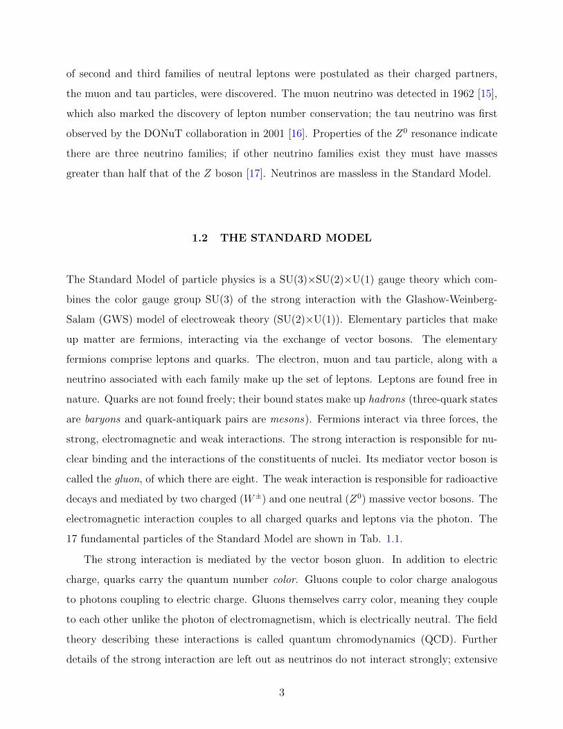
Figure 1.1: Feynman diagrams of the charged current contributions to neutrino-electron
(left) and antineutrino-electron (right) scattering.
1.2.1.1 Charged-current (CC) neutrino-electron scattering Diagrams in Fig. 1.1
show CC neutrino and antineutrino scattering from electrons. The invariant amplitude for
ν − e scattering is given by,
M =G√
2
[uνeγ
µ(1− γ5)ue] [ueγµ(1− γ5)uνe
](1.3)
Squaring this amplitude and summing over the spin states of the initial electron gives,
in the relativistic limit where me = 0,
1
2
∑spins
|M|2 = 16G2s2 (1.4)
where√s is the center-of-mass energy of the neutrino-electron system. This expression is
related to the differential scattering cross section via
dσ
dΩ=
1
64π2s
pfpi|M|2
=1
64π2s|M|2
=G2s
4π2(1.5)
6

where the pf = pi in the relativistic limit. Integrating over the isotropic solid angle distri-
bution yields,
σ(νee− → νee
−) =G2s
π(1.6)
The antineutrino-electron scattering diagram is merely the t-channel version of the neu-
trino scattering. The squared amplitude can thus be obtained by swapping s→ t:
1
2
∑spins
|M|2 = 16G2t2
= 16G2s2(1− cos2 θ) (1.7)
where θ is the angle between the ν and e− in the laboratory frame. This gives the following
expression for antineutrino-electron scattering:
dσ(νee−)
dΩ=
G2s
16π2(1− cos θ)2 ⇒ σ(νee
−) =G2s
3π(1.8)
Comparing this to Eq. (1.6) it can be seen that σ(νee−) = 1
3σ(νee
−).
d
νµ
µ−
u
W+
u
νµ µ+
d
W−
Figure 1.2: Feynman diagrams of the charged current contributions to neutrino-quark (left)
and antineutrino-quark (right) scattering.
1.2.1.2 Charged-current neutrino-quark scattering Modeling the form of the quark
weak currents in analogy with the neutrino-electron currents, we can write the amplitudes
of the diagrams in Fig. 1.2 as:
7
Mν =G√
2
[uµγµ(1− γ5)uνµ
] [uuγ
µ(1− γ5)ud]
Mν =G√
2
[uµγµ(1− γ5)uνµ
] [udγ
µ(1− γ5)uu]
(1.9)
Using Eq. (1.5) the differential quark scattering cross-section can be written as,
dσ(νµd→ µ−u)
dΩ=dσ(νµd→ µ+u)
dΩ=G2s
4π2(1.10)
dσ(νµu→ µ+d)
dΩ=dσ(νµu→ µ−d)
dΩ=
G2s
16π2(1 + cos θ)2 (1.11)
Backward scattering (i.e. θ = π) for processes of the form (1.11) is not allowed. Because
of the pure V − A structure of weak charged currents only left handed u and d (and right
handed u and d) quarks couple. Charge conservation requires that νµ do not couple to u or
d quarks while νµ do not interact with u and d type quarks.
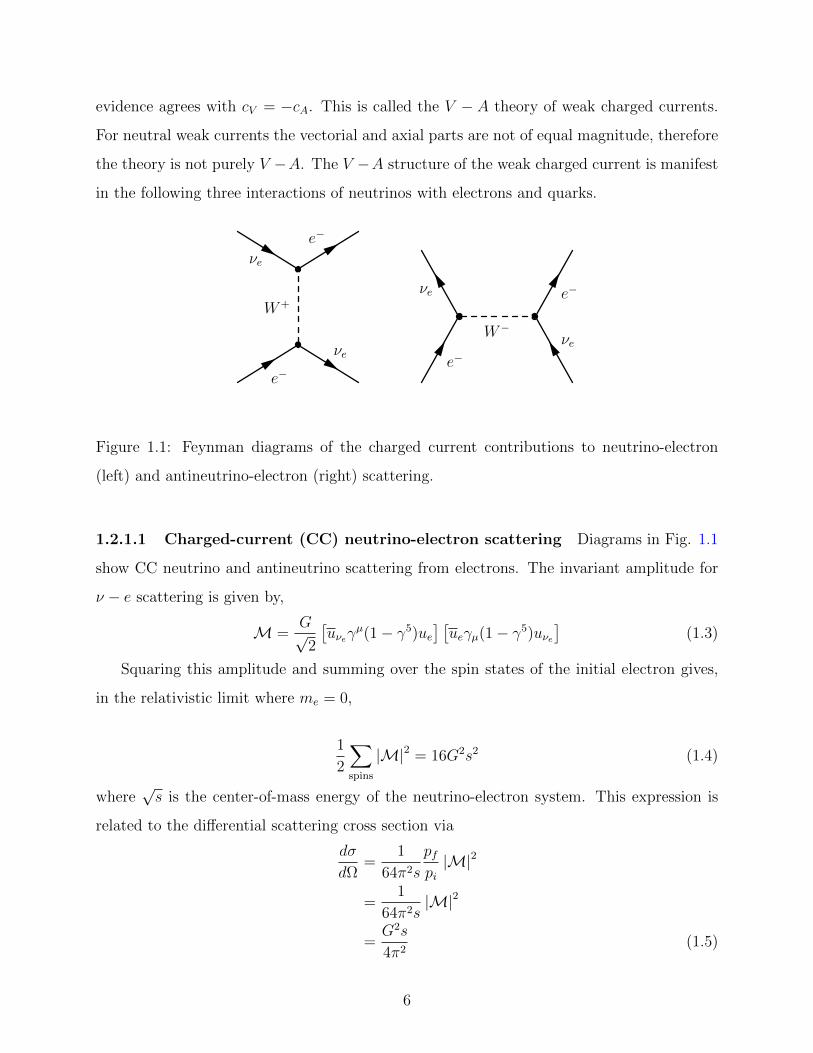
To embed the constituent ν− q scattering cross section in the experimentally observable
neutrino-nucleon (ν − N) inclusive cross-section the following Lorentz-invariant kinematic
quantities are defined:
• Energy transfer to the hadronic system
ν =p · qM
(1.12)
• Negative squared four-momentum of the exchange boson
Q2 = −q2 = −(k1 − k2)2 (1.13)
• Inelasticity
y =p · qp · k1
(1.14)
• Bjorken scaling variable
x =Q2
2p · q(1.15)
• Squared center of mass energy of the neutrino-nucleon system
s = (p+ k1)2 (1.16)
8

where k1, k2, q, p are the 4-momenta of the neutrino, muon, W and the nucleon respectively.
M is the mass of the nucleon. In the laboratory frame 1,
x =Q2
2Mν
1− y =1
2(1 + cos θ) (1.17)
where θ is the scattering angle in the lab frame. The constituent quarks carry a fraction xs
of the center of mass momentum of the system, with which the cross-sections of Eq. (1.11)
can be written:
dσ(νµd→ µ−u)
dy=G2xs
4π(1.18)
dσ(νµu→ µ+d)
dy=G2xs
4π(1− y)2 (1.19)
The neutrino-nucleon scattering inclusive cross section is given by
dσ(νN → µX)
dxdy=∑i
fi(x)
(dσidy
)(1.20)
where X is the hadronic shower and fi(x) are the parton distribution functions of the up and
down quarks in the nucleon. Neutrinos only interact with d and u quarks. Assuming there
are equal numbers of protons and neutrons in matter, the parton distribution functions can
be given as:
dproton(x) + dneutron(x) = dproton(x) + uproton(x) ≡ Q(x) (1.21)
uproton(x) + uneutron(x) = uproton(x) + dproton
(x) ≡ Q(x) (1.22)
where Q(x) and Q(x) denote the quark and antiquark distributions in matter respectively.
With these distribution functions the expression in (1.20) can be expanded to:
1x is an invariant quantity for which the following equality holds in all frames
9
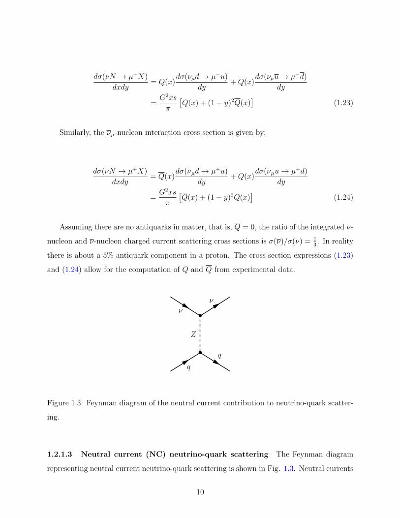
dσ(νN → µ−X)
dxdy= Q(x)
dσ(νµd→ µ−u)
dy+Q(x)
dσ(νµu→ µ−d)
dy
=G2xs
π
[Q(x) + (1− y)2Q(x)
](1.23)
Similarly, the νµ-nucleon interaction cross section is given by:
dσ(νN → µ+X)
dxdy= Q(x)
dσ(νµd→ µ+u)
dy+Q(x)
dσ(νµu→ µ+d)
dy
=G2xs
π
[Q(x) + (1− y)2Q(x)
](1.24)
Assuming there are no antiquarks in matter, that is, Q = 0, the ratio of the integrated ν-
nucleon and ν-nucleon charged current scattering cross sections is σ(ν)/σ(ν) = 13. In reality
there is about a 5% antiquark component in a proton. The cross-section expressions (1.23)
and (1.24) allow for the computation of Q and Q from experimental data.
q
ν
q
Z
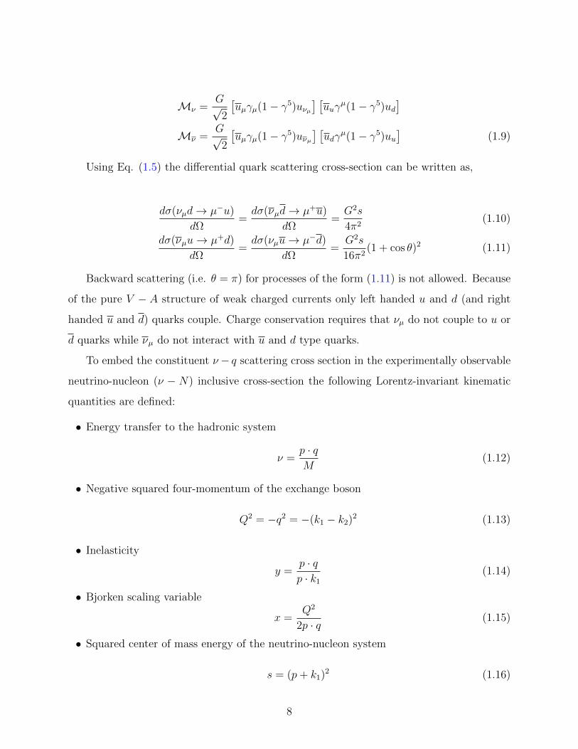
ν
Figure 1.3: Feynman diagram of the neutral current contribution to neutrino-quark scatter-
ing.
1.2.1.3 Neutral current (NC) neutrino-quark scattering The Feynman diagram
representing neutral current neutrino-quark scattering is shown in Fig. 1.3. Neutral currents
10
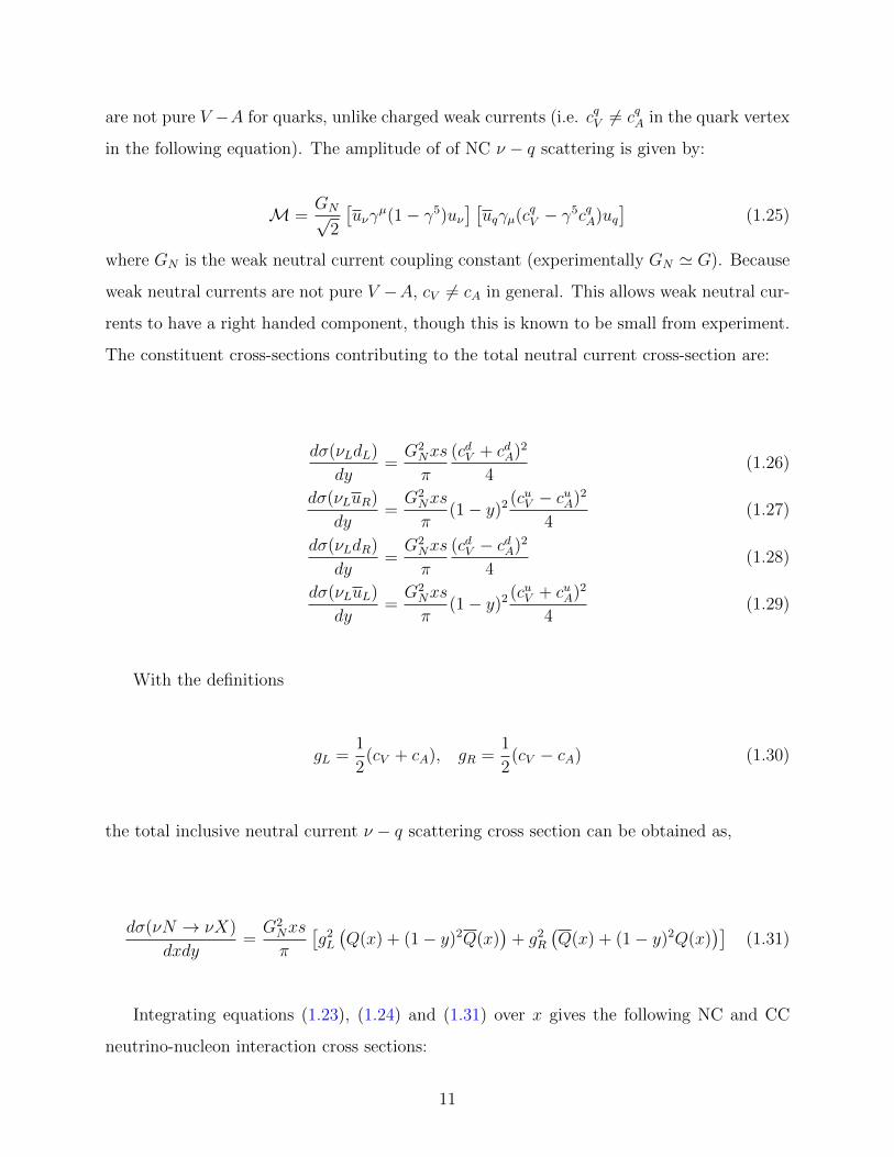
are not pure V −A for quarks, unlike charged weak currents (i.e. cqV 6= cqA in the quark vertex
in the following equation). The amplitude of of NC ν − q scattering is given by:
M =GN√
2
[uνγ
µ(1− γ5)uν] [uqγµ(cqV − γ
5cqA)uq]
(1.25)
where GN is the weak neutral current coupling constant (experimentally GN ' G). Because
weak neutral currents are not pure V −A, cV 6= cA in general. This allows weak neutral cur-
rents to have a right handed component, though this is known to be small from experiment.
The constituent cross-sections contributing to the total neutral current cross-section are:
dσ(νLdL)
dy=G2Nxs
π
(cdV + cdA)2
4(1.26)
dσ(νLuR)
dy=G2Nxs
π(1− y)2 (cuV − cuA)2
4(1.27)
dσ(νLdR)
dy=G2Nxs
π
(cdV − cdA)2
4(1.28)
dσ(νLuL)
dy=G2Nxs
π(1− y)2 (cuV + cuA)2
4(1.29)
With the definitions
gL =1
2(cV + cA), gR =
1
2(cV − cA) (1.30)
the total inclusive neutral current ν − q scattering cross section can be obtained as,
dσ(νN → νX)
dxdy=G2Nxs
π
[g2L
(Q(x) + (1− y)2Q(x)
)+ g2
R
(Q(x) + (1− y)2Q(x)
)](1.31)
Integrating equations (1.23), (1.24) and (1.31) over x gives the following NC and CC
neutrino-nucleon interaction cross sections:
11

dσNC(ν)
dy=G2Ns
π
gL[Q+ (1− y)2Q
]+ gR
[Q+ (1− y)2Q
]dσNC(ν)
dy=G2Ns
π
gL[Q+ (1− y)2Q
]+ gR
[Q+ (1− y)2Q
]dσCC(ν)
dy=G2s
π
[Q+ (1− y)2Q
]dσCC(ν)
dy=G2s
π
[Q+ (1− y)2Q
](1.32)
While weak neutral currents are not purely V − A, gR is calculated and experimentally
measured to be small. On the other hand, CC interactions are believed to be purely V −A.
1.2.2 The Electroweak Interaction
In order to convert weak interactions to a renormalizable theory, weak currents need to form
a symmetry group. The weak charge-raising and charge-lowering currents can be written,
J+µ = χLγµτ+χL (1.33)
J−µ = χLγµτ−χL (1.34)
(1.35)
where
χL =
νL
l−
L
(1.36)
is the lepton doublet and τ± = 12(τ1 ± τ2) are the tau matrices, with Pauli spin matrices τi.
The charged currents form an SU(2) isospin triplet with the following neutral current
J3µ = χLγµ
1
2τ3χL
=1
2νlLγµνlL − lLγµlL. (1.37)
12

This current can be seen to have only a left-handed component unlike the neutral current
of ν − q scattering, which has a non-zero right-handed component. The electromagnetic
current has both left- and right-handed components, and can be incorporated into the above
neutral current by the definition of a weak hypercharge current such that,
jemµ = J3µ + jYµ (hypercharge). (1.38)
This expands the symmetry group to SU(2)L×U(1)Y . Two symmetry groups require two
coupling constants, therefore a constant is needed in addition to e. To develop electroweak
theory analogous to QED, it is assumed that electroweak currents are coupled to vector
bosons just as the electromagnetic current is coupled to the photons: a triplet of vector
fields W iµ coupled to J iµ with strength g and a singlet vector field Bµ coupled to the weak
hypercharge current jYµ with strength g′/2:
−igJ iµW iµ − i
g′
2jY µBµ (1.39)
where W± =√
12(W 1
µ ∓W 2µ) are the massive charged bosons and W 3
µ and Bµ are the neutral
fields.
The electromagnetic current is a combination of J3µ and jYµ and the physical states Aµ
and Zµ are mixtures of the neutral gauge fields W 3µ and Bµ with mixing angle θW :
Aµ = Bµ cos θW +W 3µ sin θW
Zµ = −Bµ sin θW +W 3µ cos θW (1.40)
With Eq. (1.40) the electroweak neutral current becomes,
− i
(g sin θWJ
3µ + g′ cos θW
jYµ2
)Aµ
− i
(g cos θWJ
3µ − g′ cos θW
jYµ2
)Zµ (1.41)
13
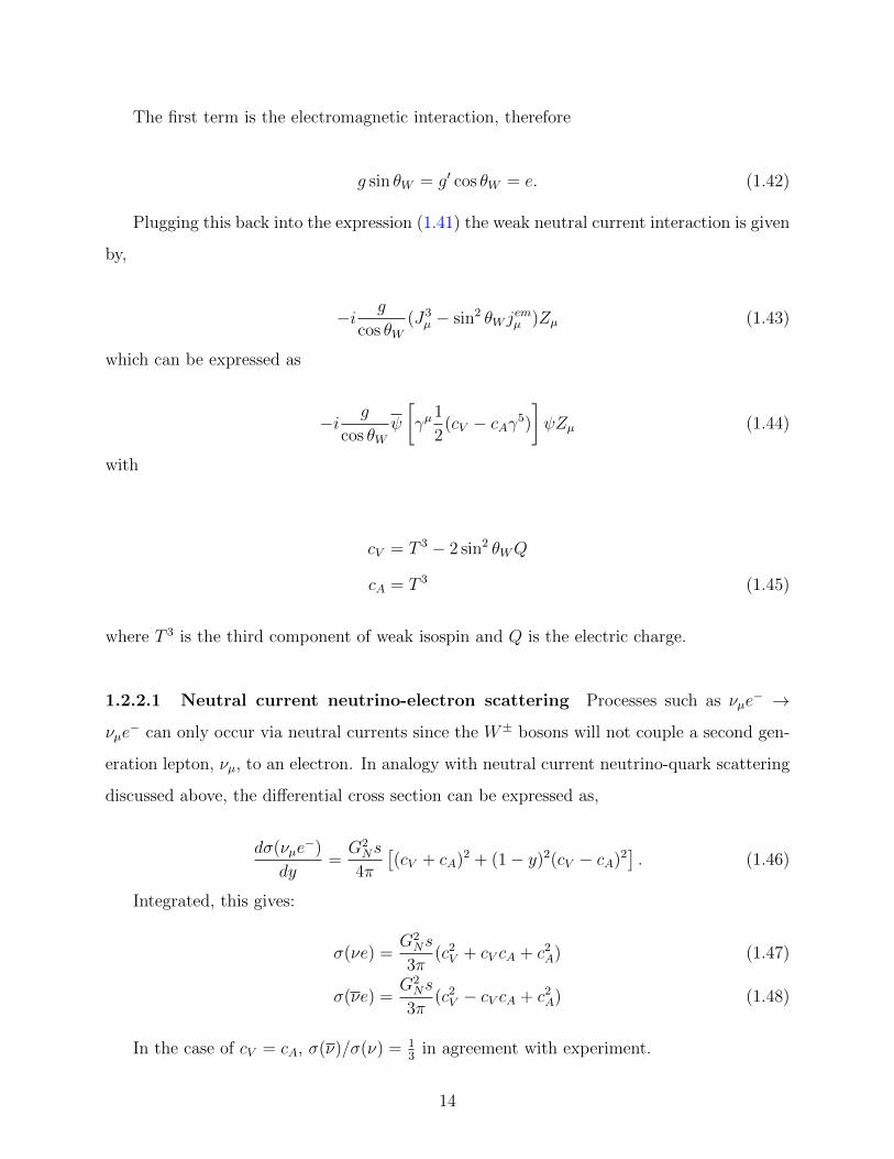
The first term is the electromagnetic interaction, therefore
g sin θW = g′ cos θW = e. (1.42)
Plugging this back into the expression (1.41) the weak neutral current interaction is given
by,
−i g
cos θW(J3µ − sin2 θW j
emµ )Zµ (1.43)
which can be expressed as
−i g
cos θWψ
[γµ
1
2(cV − cAγ5)
]ψZµ (1.44)
with
cV = T 3 − 2 sin2 θWQ
cA = T 3 (1.45)
where T 3 is the third component of weak isospin and Q is the electric charge.
1.2.2.1 Neutral current neutrino-electron scattering Processes such as νµe− →
νµe− can only occur via neutral currents since the W± bosons will not couple a second gen-
eration lepton, νµ, to an electron. In analogy with neutral current neutrino-quark scattering
discussed above, the differential cross section can be expressed as,
dσ(νµe−)
dy=G2Ns
4π
[(cV + cA)2 + (1− y)2(cV − cA)2
]. (1.46)
Integrated, this gives:
σ(νe) =G2Ns
3π(c2V + cV cA + c2
A) (1.47)
σ(νe) =G2Ns
3π(c2V − cV cA + c2
A) (1.48)
In the case of cV = cA, σ(ν)/σ(ν) = 13
in agreement with experiment.
14

1.3 NEUTRINO MIXING AND MASS
The concept of neutrino flavor change allowed by massive neutrinos was first considered by
Bruno Pontecorvo [21]. His oscillation model suggested a transition of the type ν ν:
at the time only one lepton family was known. When the muon neutrino was discovered
he considered transitions from electron to muon flavor as well. The formalism of neutrino
mixing was developed in 1962 by Ziro Maki, Masami Nakagawa and Shoichi Sakata as a two
flavor model [22]. The following discussion first generalizes this to an arbitrary number of
neutrino families then considers the special cases of three and two flavors.
Neutrino oscillations occur because neutrino flavor eigenstates |να〉 are not identical to
mass eigenstates |νi〉 but mixtures of them. Neutrinos interact via the weak interaction in
flavor eigenstates and propagate in vacuum in mass eigenstates. In the following discussion
Greek subscripts denote flavor eigenstates and Latin subscripts denote mass eigenstates.
A neutrino which is created at time t = 0 in a weak flavor |να(0)〉 eigenstate can be
expressed as a sum of mass eigenstates:
|να(0)〉 =∑i
U∗αi |νi〉 (1.49)
where U is the mixing matrix.
Mass eigenstates are eigenstates of the Hamiltonian and evolve as such while the neutrino
propagates:
|να(t)〉 =∑i
U∗αieipi·x |νi〉 (1.50)
where x is the position of the neutrino and pi is the four-momentum of the mass state i.
The neutrino is detected at time t in a detector via its weak interaction, in a flavor
eigenstate 〈νβ| =∑
j Uβj 〈νj|. The overlap with the state at time t = 0 is given by:
〈νβ|να(t)〉 =∑j
∑i
UβjU∗αie
ipi·x 〈νj|νi〉
=∑i
UβiU∗αie
ipi·x. (1.51)
15

With Ei and mi denoting the energy and mass of the ith mass eigenstate and assuming
that all mass eigenstates have the same three-momemtum p,
pi · x = Eit− p · x
= t√|p|2 +m2
i − p · x. (1.52)
For ultra-relativistic neutrinos with mi << Ei we can make the assumptions t = L and
p · x = |p|L, where L is the distance traveled. With these the above expression becomes:
pi · x = |p|L(
1 +m2i
2|p|2
)− |p|L
=miL
2E. (1.53)
This gives the amplitude 〈νβ|να(L)〉 =∑
i UβiU∗αie
im2i L
2E . The probability of observing a
neutrino in flavor β after traveling a distance L can then be calculated as,
P (να → νβ) = | 〈νβ|να(L)〉 |2
=
∣∣∣∣∣∑i
UβiU∗αie
im2i L
2E
∣∣∣∣∣2
=
(∑j
U∗βjUαje−i
m2jL
2E
)(∑i
U∗βiUαie−im
2i L
2E
)
=∑i
∑j
U∗βjUβiU∗αiUαje
−i∆m2
ijL
2E (1.54)
where ∆m2ij = m2
i −m2j .
16
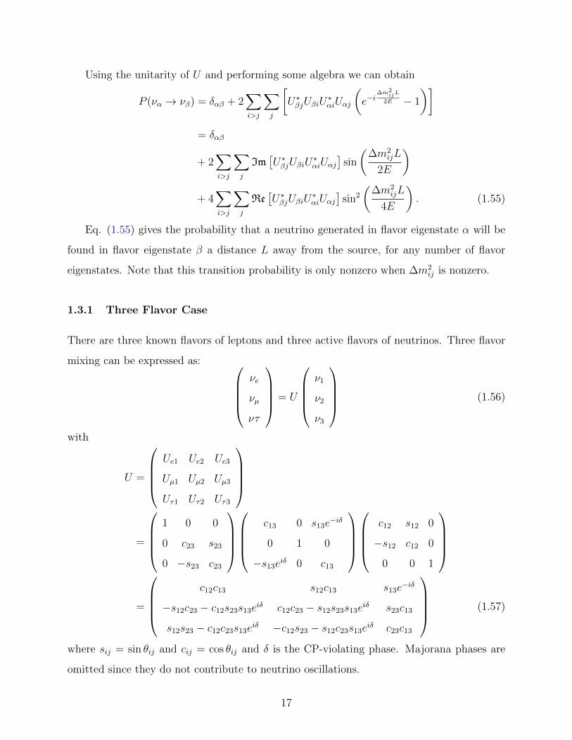
Using the unitarity of U and performing some algebra we can obtain
P (να → νβ) = δαβ + 2∑i>j
∑j
[U∗βjUβiU
∗αiUαj
(e−i
∆m2ijL
2E − 1
)]= δαβ
+ 2∑i>j
∑j
Im[U∗βjUβiU
∗αiUαj
]sin
(∆m2
ijL
2E
)
+ 4∑i>j
∑j
Re[U∗βjUβiU
∗αiUαj
]sin2
(∆m2
ijL
4E
). (1.55)
Eq. (1.55) gives the probability that a neutrino generated in flavor eigenstate α will be
found in flavor eigenstate β a distance L away from the source, for any number of flavor
eigenstates. Note that this transition probability is only nonzero when ∆m2ij is nonzero.
1.3.1 Three Flavor Case
There are three known flavors of leptons and three active flavors of neutrinos. Three flavor
mixing can be expressed as: νe
νµ
ντ
= U
ν1
ν2
ν3
(1.56)
with
U =
Ue1 Ue2 Ue3
Uµ1 Uµ2 Uµ3
Uτ1 Uτ2 Uτ3
=
1 0 0
0 c23 s23
0 −s23 c23
c13 0 s13e−iδ
0 1 0
−s13eiδ 0 c13
c12 s12 0
−s12 c12 0
0 0 1
=
c12c13 s12c13 s13e
−iδ
−s12c23 − c12s23s13eiδ c12c23 − s12s23s13e
iδ s23c13
s12s23 − c12c23s13eiδ −c12s23 − s12c23s13e
iδ c23c13
(1.57)
where sij = sin θij and cij = cos θij and δ is the CP-violating phase. Majorana phases are
omitted since they do not contribute to neutrino oscillations.
17

1.3.2 Two Flavor Case
Because of the large difference between the two mass splittings, experiments such as MINOS
are sensitive to the mixing between two of the three flavors which justifies the following two
flavor approximation:
νµ
ντ
=
cos θ sin θ
− sin θ cos θ
ν2
ν3
(1.58)
By the same arguments and approximations that led to Eq. (1.55) in the general n-flavor
case, with two flavors a state |ν(0)〉 = |νµ〉 = cos θ |ν2〉 + sin θ |ν3〉 will evolve in time t, or
equivalently path length traveled, L, to
|ν(L)〉 = |νµ〉 = cos θ exp
(−im
22L
2E
)|ν2〉+ sin θ exp
(−im
23L
2E
)|ν3〉 . (1.59)
The probability that it will be detected with the same flavor after traveling this distance
is given by
Pνµ→νµ = |〈νµ |ν(L)〉|2 =
∣∣∣∣cos2 θ e−im2
2L
2E + sin2 θ e−im2
3L
2E
∣∣∣∣2= 1− 2 cos2 θ sin2 θ
[1− cos
(∆m2
23L
2E
)]= 1− sin2 2θ
[2 sin2
(∆m2
23L
4E
)]. (1.60)
In SI units with c and ~ restored the argument of the sine becomes
∆m223c
4L
4E~c= 1.27
∆m223L
E
[eV2 · km
GeV
]. (1.61)
Substituting this into Eq. (1.60) gives the survival probability relevant to MINOS
Pνµ→νµ = 1− sin2 (2θ23) sin2
(1.27
∆m223L
E
). (1.62)
18
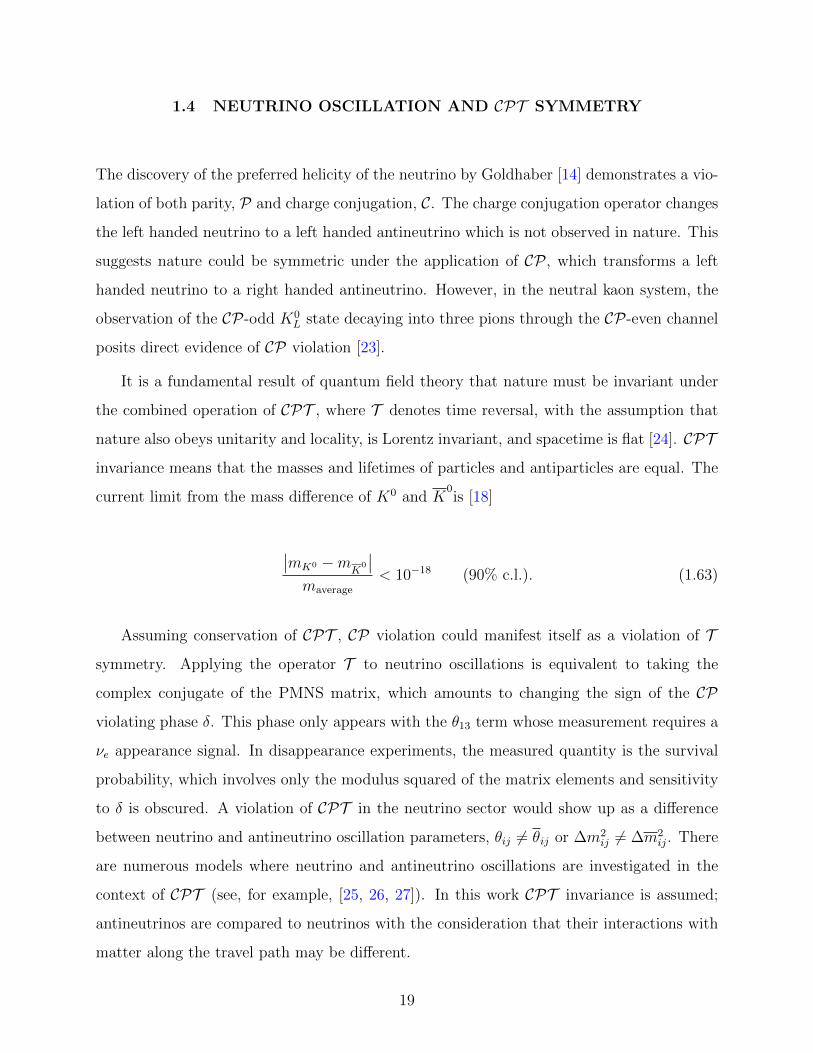
1.4 NEUTRINO OSCILLATION AND CPT SYMMETRY
The discovery of the preferred helicity of the neutrino by Goldhaber [14] demonstrates a vio-
lation of both parity, P and charge conjugation, C. The charge conjugation operator changes
the left handed neutrino to a left handed antineutrino which is not observed in nature. This
suggests nature could be symmetric under the application of CP , which transforms a left
handed neutrino to a right handed antineutrino. However, in the neutral kaon system, the
observation of the CP-odd K0L state decaying into three pions through the CP-even channel
posits direct evidence of CP violation [23].
It is a fundamental result of quantum field theory that nature must be invariant under
the combined operation of CPT , where T denotes time reversal, with the assumption that
nature also obeys unitarity and locality, is Lorentz invariant, and spacetime is flat [24]. CPT
invariance means that the masses and lifetimes of particles and antiparticles are equal. The
current limit from the mass difference of K0 and K0is [18]
∣∣mK0 −mK
0
∣∣maverage
< 10−18 (90% c.l.). (1.63)
Assuming conservation of CPT , CP violation could manifest itself as a violation of T
symmetry. Applying the operator T to neutrino oscillations is equivalent to taking the
complex conjugate of the PMNS matrix, which amounts to changing the sign of the CP
violating phase δ. This phase only appears with the θ13 term whose measurement requires a
νe appearance signal. In disappearance experiments, the measured quantity is the survival
probability, which involves only the modulus squared of the matrix elements and sensitivity
to δ is obscured. A violation of CPT in the neutrino sector would show up as a difference
between neutrino and antineutrino oscillation parameters, θij 6= θij or ∆m2ij 6= ∆m2
ij. There
are numerous models where neutrino and antineutrino oscillations are investigated in the
context of CPT (see, for example, [25, 26, 27]). In this work CPT invariance is assumed;
antineutrinos are compared to neutrinos with the consideration that their interactions with
matter along the travel path may be different.
19

1.5 NEUTRINO OSCILLATIONS IN MATTER
Neutrino oscillations are altered by the presence of matter along the path of travel from
creation to detection as first shown by Lincoln Wolfenstein in 1978 [28]. The model was later
applied to the solar neutrino oscillation problem by Mikheev and Smirnov [29] and is known
as the MSW effect after its three discoverers. This effect is different for νe because matter
is predominantly composed of leptons in the first family (electrons). While all three flavors
of neutrinos experience the same neutral current scattering in matter, electron neutrinos
also scatter via charged current coherent forward scattering. In the absence of matter the
evolution of the neutrino state is expressed in the mass basis by,
i∂
∂t
ν1
ν2
= H0
ν1
ν2
(1.64)
where, for mass eigenstates the Hamiltonian is obtained
H0 =
E1 0
0 E2
≈ p+
m21
2E0
0 p+m2
2
2E
(1.65)
where p is the neutrino momentum, E is the neutrino energy, and m1 and m2 are the
masses of the eigenstates ν1 and ν2. Mass eigenstates can be expressed as flavor eigenstates
multiplied by U † from the left. Then multiplying the expression from the left by U gives,
i∂
∂t
νe
νx
= UH0U†
νe
νx
(1.66)
=
p+m2
1
2E0
0 p+m2
2
2E
νe
νx
(1.67)
Charged-current scattering of electron neutrinos from electrons in matter introduces an
additional matter potential,
Ve = ±√
2GFNe (1.68)
20
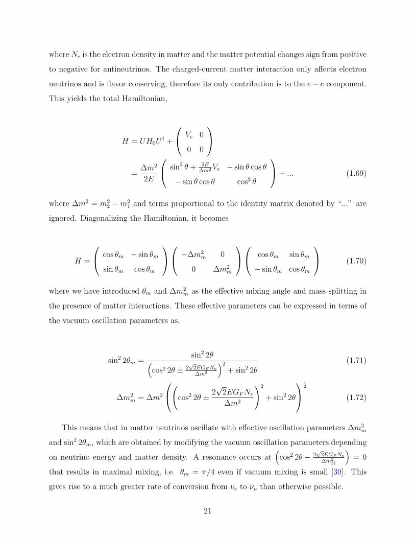
where Ne is the electron density in matter and the matter potential changes sign from positive
to negative for antineutrinos. The charged-current matter interaction only affects electron
neutrinos and is flavor conserving, therefore its only contribution is to the e− e component.
This yields the total Hamiltonian,
H = UH0U† +
Ve 0
0 0
=
∆m2
2E
sin2 θ + 2E∆m2Ve − sin θ cos θ
− sin θ cos θ cos2 θ
+ ... (1.69)
where ∆m2 = m22 −m2
1 and terms proportional to the identity matrix denoted by “...” are
ignored. Diagonalizing the Hamiltonian, it becomes
H =
cos θm − sin θm
sin θm cos θm
−∆m2m 0
0 ∆m2m
cos θm sin θm
− sin θm cos θm
(1.70)
where we have introduced θm and ∆m2m as the effective mixing angle and mass splitting in
the presence of matter interactions. These effective parameters can be expressed in terms of
the vacuum oscillation parameters as,
sin2 2θm =sin2 2θ(
cos2 2θ ± 2√
2EGFNe∆m2
)2
+ sin2 2θ(1.71)
∆m2m = ∆m2
(cos2 2θ ± 2√
2EGFNe
∆m2
)2
+ sin2 2θ
12
(1.72)
This means that in matter neutrinos oscillate with effective oscillation parameters ∆m2m
and sin2 2θm, which are obtained by modifying the vacuum oscillation parameters depending
on neutrino energy and matter density. A resonance occurs at(
cos2 2θ − 2√
2EGFNe∆m2
21
)= 0
that results in maximal mixing, i.e. θm = π/4 even if vacuum mixing is small [30]. This
gives rise to a much greater rate of conversion from νe to νµ than otherwise possible.
21

1.6 NON-STANDARD MATTER INTERACTIONS
As discussed in section 1.5, standard matter interactions affect the survival probability of
the electron neutrino but not of the muon and tau neutrinos since muon and tau particle
densities in normal matter are minuscule compared to electrons. There can be, however,
non-standard matter interactions (NSI) that influence survival probabilities of second and
third generation neutrinos. These are interactions of neutrinos with matter (up and down
quarks and electrons), standard versions of which have been discussed in Section 1.2.1. One
way in which non-standard interactions can arise is through the violation of the unitarity
of the lepton mixing matrix in certain see-saw models [31]. Sizable NSI effects can be
introduced via new scalar exchange bosons such as Higgs bosons or scalar leptoquarks, some
supersymmetric models may also give rise to NSI [32].
In general there can be charged-current NSI which affect the production and detection of
neutrinos, and neutral-current NSI which alter the propagation through matter. The general
leptonic charged current NSI Lagrangian density is given by [33],
LlNSI = −2√
2GF εγδαβ[lαγ
µ(1 + aγ5)lβ][νγγµ(1− γ5)νδ] (1.73)
where a = +/ − 1 for right/left handed leptons and α 6= β to generate flavor changing
interactions. This leptonic CC NSI is relevant to the production of neutrinos. Similarly,
non-standard charged-current interactions with quarks can be expressed by,
LuNSI = −2√
2GF εudαβVud[uγ
µ(1 + aγ5)d][lαγµ(1− γ5)νβ] + h.c. (1.74)
where matter contains only u and d quarks. Neutrinos interact with d or u quarks, an-
tineutrinos with u or d (see Section 1.2.1.2). The interaction with quarks is relevant to
the production and detection of neutrinos. In this thesis charged-current contributions to
non-standard interactions are neglected because they are strongly constrained from short-
baseline neutrino oscillation experiments [34, 35] and MINOS is not sensitive to them [36].
While in general they can be as strong as neutral-current NSI, NC NSI are enhanced by the
length of the baseline and are the only NSI interactions able to generate a detectable effect
in MINOS.
22

The neutral-current NSI Lagrangian is of the form [37],
LNSI = −GF√2
∑f=u,d,ea=±1
εfaαβ[uναγ
µ(1− γ5)uνβ] [ufγµ(1 + aγ5)uf
](1.75)
where coefficients εfαβ give the strength of the NSI effect on transitions between α and β
flavors as a result of interacting with fermion f = e, u, d. Since matter is not polarized only
the vectorial part of this interaction is non-vanishing for propagation through matter; the
NSI Lagrangian will add a term to the Hamiltonian as,
HNSI = Ve
εee εeµ εeτ
ε∗eµ εµµ εµτ
ε∗eτ ε∗µτ εττ
(1.76)
where Ve = ±√
2GFNe is the matter potential. The ε parameters have been summed over
the fermion contributions
εαβ =∑f,a
εfaαβNf
Ne
(1.77)
where Nf is the fermion density in matter.
MINOS is sensitive to oscillations in the atmospheric sector and the vacuum oscillation
model has been developed in the two-flavor approximation in section 1.3. The NSI formalism
will be discussed in such a two flavor scenario as well. The parameters that appear in the
following discussion are described as
• Real valued NSI strength parameters ε = εµτ and ε′ = εµµ − εττ
• Atmospheric mass splitting ∆m2 = ∆m232 = m2
3 −m22 and mixing angle θ = θ23
• Neutrino energy E = Eν
The two flavor Hamiltonian including NSI can be expressed as,
H =
cos(2θ)∆m2
4E+ ε′Ve sin(2θ)∆m2
4E+ εVe
sin(2θ)∆m2
4E+ εVe − cos(2θ)∆m2
4E+ ε′Ve
(1.78)
23
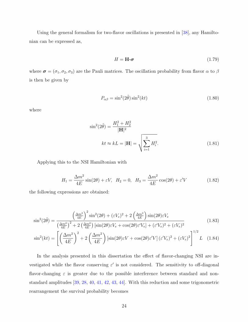
Using the general formalism for two-flavor oscillations is presented in [38], any Hamilto-
nian can be expressed as,
H = H·σ (1.79)
where σ = (σ1, σ2, σ3) are the Pauli matrices. The oscillation probability from flavor α to β
is then be given by
Pαβ = sin2(2θ) sin2(kt) (1.80)
where
sin2(2θ) =H2
1 +H22
|H|2
kt ≈ kL = |H| =
√√√√ 3∑i=1
H2i . (1.81)
Applying this to the NSI Hamiltonian with
H1 =∆m2
4Esin(2θ) + εV, H2 = 0, H3 =
∆m2
4Ecos(2θ) + ε′V (1.82)
the following expressions are obtained:
sin2(2θ) =
(∆m2
4E
)2
sin2(2θ) + (εVe)2 + 2
(∆m2
4E
)sin(2θ)εVe(
∆m2
4E
)2+ 2
(∆m2
4E
)[sin(2θ)εVe + cos(2θ)ε′Ve] + (ε′Ve)2 + (εVe)2
(1.83)
sin2(kt) =
[(∆m2
4E
)2
+ 2
(∆m2
4E
)[sin(2θ)εV + cos(2θ)ε′V ] (ε′Ve)
2 + (εVe)2
]1/2
L (1.84)
In the analysis presented in this dissertation the effect of flavor-changing NSI are in-
vestigated while the flavor conserving ε′ is not considered. The sensitivity to off-diagonal
flavor-changing ε is greater due to the possible interference between standard and non-
standard amplitudes [39, 28, 40, 41, 42, 43, 44]. With this reduction and some trigonometric
rearrangement the survival probability becomes
24
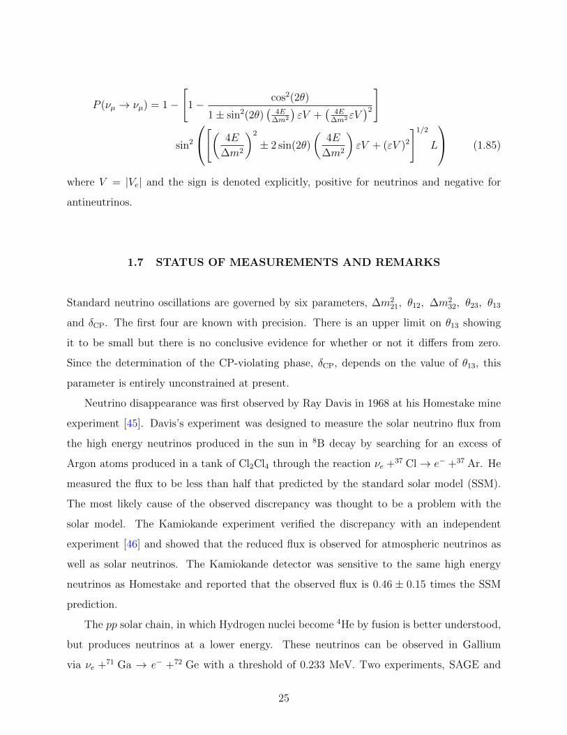
P (νµ → νµ) = 1−
[1− cos2(2θ)
1± sin2(2θ)(
4E∆m2
)εV +
(4E
∆m2 εV)2
]
sin2
[( 4E
∆m2
)2
± 2 sin(2θ)
(4E
∆m2
)εV + (εV )2
]1/2
L
(1.85)
where V = |Ve| and the sign is denoted explicitly, positive for neutrinos and negative for
antineutrinos.
1.7 STATUS OF MEASUREMENTS AND REMARKS
Standard neutrino oscillations are governed by six parameters, ∆m221, θ12, ∆m2
32, θ23, θ13
and δCP. The first four are known with precision. There is an upper limit on θ13 showing
it to be small but there is no conclusive evidence for whether or not it differs from zero.
Since the determination of the CP-violating phase, δCP, depends on the value of θ13, this
parameter is entirely unconstrained at present.
Neutrino disappearance was first observed by Ray Davis in 1968 at his Homestake mine
experiment [45]. Davis’s experiment was designed to measure the solar neutrino flux from
the high energy neutrinos produced in the sun in 8B decay by searching for an excess of
Argon atoms produced in a tank of Cl2Cl4 through the reaction νe +37 Cl→ e− +37 Ar. He
measured the flux to be less than half that predicted by the standard solar model (SSM).
The most likely cause of the observed discrepancy was thought to be a problem with the
solar model. The Kamiokande experiment verified the discrepancy with an independent
experiment [46] and showed that the reduced flux is observed for atmospheric neutrinos as
well as solar neutrinos. The Kamiokande detector was sensitive to the same high energy
neutrinos as Homestake and reported that the observed flux is 0.46 ± 0.15 times the SSM
prediction.
The pp solar chain, in which Hydrogen nuclei become 4He by fusion is better understood,
but produces neutrinos at a lower energy. These neutrinos can be observed in Gallium
via νe +71 Ga → e− +72 Ge with a threshold of 0.233 MeV. Two experiments, SAGE and
25

GALLEX, performed this measurement in the 1990s [47, 48] and confirmed that the observed
flux is about half that of the SSM prediction. Kamiokande and later its upgrade with larger
fiducial volume, Super-Kamiokande, kept confirming that the measured νe flux is half of the
SSM prediction [49, 50]: this came to be known as the “solar neutrino problem.”
The SNO [51] experiment could differentiate between CC and NC interactions. Only νe
participate in the former while all flavors participate equally in the latter. This confirmed
that the total flux is in agreement with the SSM prediction while the number of electron
neutrinos is lower than expected, demonstrating agreement with both the SSM and neutrino
flavor change.
Another way of measuring neutrino oscillations in the “solar” sector is the detection of
νe from other sources. Nuclear reactors provide a flux of νe and KamLAND is one of the
early experiments to detect reactor antineutrinos [52]. The KamLAND detector in Japan is
sensitive to the same region as the solar neutrino experiments above. Fig. 1.4 shows contours
from solar experiments along with KamLAND results. The combined fit to all existing data
in the solar sector yields the best world measurement of
∆m221 = (7.59± 0.20)× 10−5eV2, tan2 θ12 = 0.470.06
0.05. (1.86)
The mixing angle is near maximal, and this region is dubbed the large mixing angle
(LMA) region. From the sign of MSW matter effects, solar neutrino oscillation measurements
indicate that m2 > m1.
The second set of oscillation parameters, ∆m232 and θ23, are measured from atmospheric
neutrinos and accelerator based νµ beams. Pions and kaons are produced when cosmic rays
strike the atmosphere and they decay into neutrinos via, primarily, π+ → µ+ + νµ; µ+ →
e+ + νe + νµ. Therefore, it is natural to expect a νµ : νe flux ratio of 2:1. However, a
similar discrepancy to the solar neutrino anomaly was observed when experiments confirmed
the expected νe rate but reported that the νµ flux was 23
the prediction [53]. Atmospheric
neutrino oscillation is now a well established phenomenon with precision measurements of
the parameters governing it. The most recent and precise measurement using neutrinos from
26

Figure 1.4: Allowed regions for neutrino oscillations from combined solar experiments and
KamLAND. The side panels show the ∆χ2 profiles. From [52].
the atmosphere come from Super-Kamiokande (assuming m3 > m1,2) [54]
1.9× 10⁻³ ≤ |∆m2atm| ≤ 2.6× 10⁻³ eV2 (90% C.L) (1.87)
0.407 ≤ sin2 θ23 ≤ 0.583 (90% C.L) (1.88)
with best fit values |∆m2atm| = 2.1× 10⁻³ eV2 and sin2 θ23 = 0.5.
These results are confirmed by experiments using manmade atmospheric neutrinos, that
27
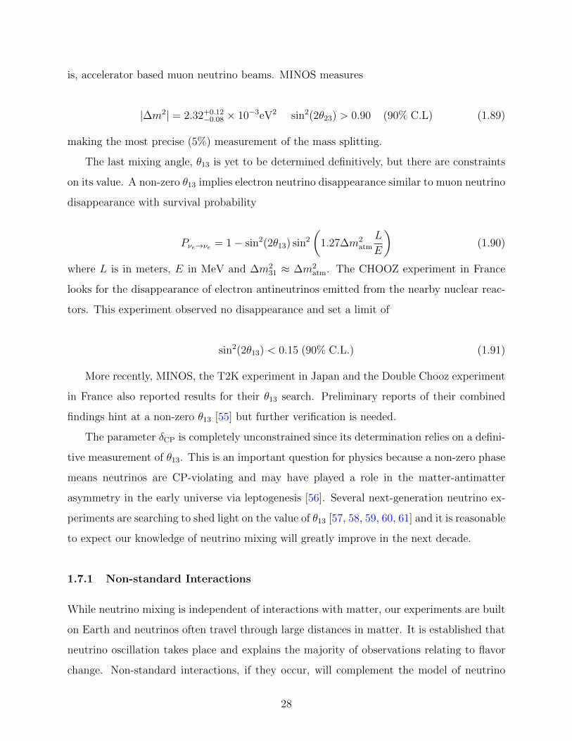
is, accelerator based muon neutrino beams. MINOS measures
|∆m2| = 2.32+0.12−0.08 × 10⁻³eV2 sin2(2θ23) > 0.90 (90% C.L) (1.89)
making the most precise (5%) measurement of the mass splitting.
The last mixing angle, θ13 is yet to be determined definitively, but there are constraints
on its value. A non-zero θ13 implies electron neutrino disappearance similar to muon neutrino
disappearance with survival probability
Pνe→νe = 1− sin2(2θ13) sin2
(1.27∆m2
atm
L
E
)(1.90)
where L is in meters, E in MeV and ∆m231 ≈ ∆m2
atm. The CHOOZ experiment in France
looks for the disappearance of electron antineutrinos emitted from the nearby nuclear reac-
tors. This experiment observed no disappearance and set a limit of
sin2(2θ13) < 0.15 (90% C.L.) (1.91)
More recently, MINOS, the T2K experiment in Japan and the Double Chooz experiment
in France also reported results for their θ13 search. Preliminary reports of their combined
findings hint at a non-zero θ13 [55] but further verification is needed.
The parameter δCP is completely unconstrained since its determination relies on a defini-
tive measurement of θ13. This is an important question for physics because a non-zero phase
means neutrinos are CP-violating and may have played a role in the matter-antimatter
asymmetry in the early universe via leptogenesis [56]. Several next-generation neutrino ex-
periments are searching to shed light on the value of θ13 [57, 58, 59, 60, 61] and it is reasonable
to expect our knowledge of neutrino mixing will greatly improve in the next decade.
1.7.1 Non-standard Interactions
While neutrino mixing is independent of interactions with matter, our experiments are built
on Earth and neutrinos often travel through large distances in matter. It is established that
neutrino oscillation takes place and explains the majority of observations relating to flavor
change. Non-standard interactions, if they occur, will complement the model of neutrino
28
mixing and oscillation. NSI models are purely phenomenological, currently with no estab-
lished theory asserting the physics that gives rise to them. It is therefore essential to search
for NSI in a model independent manner; the parametrization in Section 1.6 satisfies this.
Much like oscillations, there is not one experiment that can search for NSI in all sectors.
Multiple experiments contribute to the constraints on εαβ for each α, β. The interpretation of
these reports depends on the matter through which neutrinos traveled and which particles in
said matter were included in the analysis. Baselines of experiments range from a few hundred
meters to the Earth’s diameter. For neutrinos traveling through the Earth’s mantle and core
as well as the crust, density variations are significant and MSW resonances in the denser
mantle and core may become non-negligible. Through the MINOS baseline neutrinos remain
in the crust, whose average density is taken to be ρ = 2.72g/cm3, giving Ve = 1.1× 10⁻¹³eV.
An analysis can search for NSI parameters, ε, corresponding to interactions with u, d
quarks and electrons separately, or reduce them to the effective parameters which are summed
over the contributions of the three fermions present in regular matter. When comparing
results from two methods they need to be scaled accordingly [62]. In this dissertation we
treat ε as the effective NSI parameter summed over electrons, and up and down quarks (see
Sec. 1.6), though down quarks dominate because of the larger interaction cross section and
the work presented here is comparable to those experiments that make the assumption that
only d-quarks contribute to NSI.
A comprehensive and inclusive analysis [33] gives the following bounds on all neutral-
current NSI through Earth matter:
|εαβ| ≤
4.2 0.33 3.0
0.33 0.068 0.33
3.0 0.33 21
(1.92)
where εµτ < 0.33 is the parameter MINOS is measuring. Eq. (1.92) is a reliable order-of-
magnitude estimate of the knowledge of upper limits for non-standard interactions. There are
reports from single experiments or global fits that make more stringent claims with a variety
of assumptions [63, 64]; most recent and most similar to the analysis presented in this thesis
is a measurement the Super-K experiment reported of a search for non-standard interactions.
29

In contrast to MINOS,which is sensitive to NSI primarily through the sign change of the
matter potential, V , due to its ability to distinguish neutrinos and antineutrinos, Super-K
cannot identify the charge of the muon but is sensitive to NSI because of its much wider
range of L/E. The two experiments’ NSI analyses are therefore complementary. Super-K
observes no non-standard interactions and sets the following limits on NSI parameters [65]:
|εµτ | < 1.1× 10⁻²
−4.9× 10⁻² < εττ − εµµ < 4.9× 10⁻² (1.93)
Most of the constraints on NSI parameters are comparable to MINOS’s sensitivity to
non-standard interactions. This work is a valuable contribution to understanding NSI since
it comes from a single experiment where systematic uncertainties and experimental factors
are well understood and controlled.
30
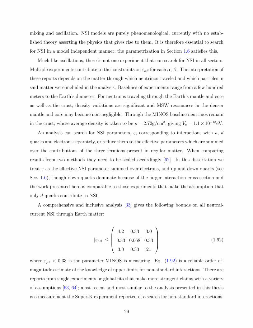
2.0 THE MINOS BEAM AND DETECTORS
The MINOS Experiment is made up of the NuMI (Neutrinos at the Main Injector) high
intensity neutrino beam and two nearly identical tracking calorimeters: The Near Detector
at Fermilab and the Far Detector in the Soudan Mine in Northern Minnesota. Side and top
views of the detectors’ locations are shown in Fig. 2.1.
10 km
12 km 735 km
Fermilab Soudan
Figure 2.1: Side view (left) and bird’s eye view diagrams of the locations of the MINOS
detectors. Due to the Earth’s curvature the beam is aimed downwards, travels through the
crust to Soudan and exits the surface to the north of the Far Detector. The figure is adapted
from [66].
31

2.1 THE NUMI BEAM
The NuMI beam, a schematic of which is shown in Fig. 2.2, is generated at Fermilab by
using protons from the Main Injector (MI). The MI delivers 120 GeV protons in a series of
pulses, also called spills, each of which contains six batches. Of these six, NuMI receives
five or six batches with the remaining one going to produce antiprotons for the Tevatron.
A spill of protons arrives on average every 2.2 seconds and lasts for 10µs. The typical spill
intensity is 36 × 1012 protons per pulse (ppp) when the Tevatron is also using the MI, and
upwards of 40× 1012 ppp when the accelerator runs in NuMI-only mode. The proton beam
is aimed 58 mrad downwards into the Earth by quadrupole and bending magnets to point at
the Far Detector, which resides in an underground mine. The downward angle is necessary
because of the curvature of the Earth. After passing through a series of beam monitoring
devices, the proton beam reaches a baffle just upstream of the NuMI target. The baffle, a 150
cm-long rod with a central aperture of radius 11 mm, protects the downstream components
by reducing the intensity of poorly focused protons.
Figure 2.2: A schematic of the NuMI beamline. Protons from the Main Injector strike the
graphite target; particles produced from this are focused by a two magnetic horns into the
decay pipe where mesons decay into muons and muons neutrinos. Muons and undecayed
hadrons range out through a series of absorbers and monitors; the neutrino beam continues
to the detectors. Figure taken from [67].
32

The protons then strike a segmented, water-cooled, graphite target. The target consists
of 47 segments of 6.4 mm width, 15 m height and 20 mm length, with 0.3 mm spacing. This
gives the target a total length of 954 mm which corresponds to 1.9 interaction lengths. The
graphite is water cooled by pipes running at the top and bottom of each segment. Fig. 2.3
shows the target and its enclosure.
!!"#"$% &'()*+%!"#$!%$&'()%*!+$,-!).!/(*0&1$0!+2!/)*%!0$1,23!!"#*.$!/)*%.!,($!/(*0&1$0!+2!)%'$(,1')*%.!*4!'#$!/()-,(2!/(*'*%!+$,-!5)'#!'#$!',(6$'3!!"#$!/(*'*%!+$,-!./*'!.)7$!.#*&80!+$!%*!.-,88$(!'#,%!93:!--!;<=!#*()7*%',882!,%0!>$(')1,882!,'!4&88!+,.$8)%$!+$,-!)%'$%.)'2!'*!8)-)'!+$,-!)%0&1$0!.'($..!*%!'#$!',(6$'3!!"#$! ',(6$'! -,'$(),8! ).! 6(,/#)'$?! '2/$! @ABCDE! FGHIH! J(,/#)'$K?! 0$%.)'2! 93LM! 6N1-O3! ! "#$!6(,/#)'$! .$6-$%'.! ,($! -,1#)%$0! ,.! %,((*5! 4)%.! ,%0! -*&%'$0! '*! .',)%8$..! .'$$8! 5,'$(C1**8)%6!/)/$.?!,.!.#*5%!)%!,-).(*%!"#/0#!,%0!,-).(*%!"#/0$3!!"#$!,)(')6#'!1,.)%6!#,.!+$(288)&-!5)%0*5.!4*(!'#$!/()-,(2!+$,-!$%'(,%1$!,%0!$P)'3!!"#$!-,)%!',(6$'!).!QL!>$(')1,8!',(6$'!.$6-$%'.?!$,1#!R:3:!--!8*%6?!5)'#!:3O!--!./,1)%6!+$'5$$%!.$6-$%'.?!4*(!,!'*',8!8$%6'#!*4!SD3OM!1-3!!"#$!.$6-$%'.!,($!T3Q!--!5)0$3!!"#$!#$)6#'!).!.1&8/'$0!F.$$!B)6&($!RK3!!U!QM'#!.$6-$%'!F%*'!.#*5%K!).!-*&%'$0!#*()7*%',882?!)%!'#$!',(6$'!1,%).'$(?!5)'#!'#$!4)%!1$%'$(!9DL3O!--!&/.'($,-!*4!'#$!&/.'($,-!$06$!*4!'#$!-,)%!',(6$'3!
,-).(*%!"#/0#!!"#$!',(6$'!,%0!',(6$'!>,1&&-!1,%).'$(3!!!
!
Figure 2.3: The NuMI target casing and components. The proton beam enters through the
window in the target canister shown on the left hand side. The target is segmented as shown
(not to scale) and cooled by two water pipes on either side. The segments are contained in
an aluminum casing. Taken from [66].
The interaction of protons with the graphite target produces a variety of daughter par-
ticles including charged mesons (pions and kaons),
p+ C → π±, K± +X (2.1)
These particles are focused by two magnetic horns that produce a toroidal magnetic
field about an axis along the beam direction. The parabolic shape of the inner conductor
makes the magnetic field act as a thin lens with focal length proportional to the meson’s
momentum, allowing momentum-selective focusing. The target is mounted at the upstream
end of the first horn, sitting inside it. Most mesons are traveling parallel to the beam axis
as they exit the horns.
33

The decay pipe is a 675 m long steel pipe with a diameter of 2 meters where the mesons
decay into muons and muon neutrinos:
π+(−) → νµ(νµ) + µ+(−),
K+(−) → νµ(νµ) + µ+(−). (2.2)
The decay pipe was evacuated to down to about 1 Torr for the first two runs of the
experiment. Data from subsequent runs were collected with the decay pipe filled with Helium
gas at 0.9 atm. The decision to fill the decay pipe with Helium gas was taken in order to
prevent a potential implosion which became a significant risk. The presence of He in the
decay pipe results in a slight decrease in the focusing peak as some mesons interact with the
gas before they can decay. It also acts as an additional meson production target resulting in
a small increase in the flux above the focusing peak.
The beam goes through a hadron absorber following the decay pipe where undecayed
mesons and uninteracted protons get absorbed. The muons range out to 240 meters of
rock after the absorber where they, too, get stopped. There is one hadron monitor directly
upstream of the hadron absorber and three muon monitors, placed in the rock that follows
the absorber, alternating with layers of rock. The beam then reaches the Near Detector.
Muons from interactions with the rock just upstream of the detector also enter through the
detector face. In this forward horn current (FHC) focusing mode the beam detected by
the Near Detector is composed of 91.7% νµ, 7% νµ and 1.3% (νe + νe). The antineutrino
component comes from negative mesons traveling through the center of the horns that do
not get deflected. The electron flavor component is due to secondary decays of muons. The
Near Detector spectra of muon neutrinos and antineutrinos in FHC-mode are shown in Fig.
2.5.
In order to make an antineutrino beam, the polarity of the horn current is reversed to
focus negatively charged mesons which decay into antineutrinos. Cartoons of forward horn
current (FHC) neutrino-mode and reversed horn current (RHC) antineutrino-mode focusing
are shown in Fig. 2.4. The composition of the reversed horn current (RHC) beam integrated
over all energies is 40% νµ, 58% νµ and 2% electron flavored. The spectra in this mode are
34

shown in Fig.2.6. Neutrino Mode!
120 GeV protons from MI!
Focusing Horns!
2 m
675 m!15 m! 30 m!
!
"µ = 91.7%" µ = 7.0%
"e +" e =1.3%
Target! Decay Pipe!
!-
!+ "µ
Monte Carlo!Neutrino mode Horns focus !+, K+
"µ/"µ
Antineutrino Mode!
!+
!-
Target! Focusing Horns! Decay Pipe!
2 m
675 m!
"µ
15 m! 30 m!
120 GeV protons from MI!
Monte Carlo!Neutrino mode Horns focus !+, K+
!
"µ = 91.7%" µ = 7.0%
"e +" e =1.3%
Monte Carlo!Antineutrino mode Horns focus !-, K-
!
" µ = 39.9%"µ = 58.1%
"e +" e = 2.0%
"µ/"µ
Figure 2.4: The sketches show the upstream part of the beamline geometry and focusing
optics in forward (top) and reversed horn current modes. Figures taken from [68].
35

True Energy (GeV)0 5 10 15 20 25 30
(Arb
itrar
y Un
its)
CCσ ×
Flux
0
0.2
0.4
0.6
0.8
1
MINOS Preliminary
Near DetectorSimulatedLow Energy Beam
Spectrumµν Spectrumµν
Forward Horn Current
Figure 2.5: Simulated Near Detector energy spectra of muon neutrinos and antineutrinos in
forward horn current mode.
True Energy (GeV)0 5 10 15 20 25 30
(Arb
itrar
y U
nits
)C
Cσ ×
Flux
0
0.2
0.4
0.6
0.8
1
MINOS Preliminary
Near DetectorSimulatedLow Energy Beam
Spectrumµν Spectrumµν
Reversed Horn Current
Figure 2.6: Simulated Near Detector energy spectra of muon neutrinos and antineutrinos in
reversed horn current mode.
36

Reversing the horn polarity changes the spectra of signal and background because of the
combination of two effects; first the beam is produced by protons which results in a larger
flux of positively charged mesons and second, the interaction cross section of antineutrinos
with the Near Detector is about half that of neutrinos [69, 70]. This results in a smaller flux
compared to neutrino-mode.
The NuMI beamline can be operated in multiple configurations. The peak energy of the
neutrino beam can be adjusted by varying the target position relative to the horns. Fig. 2.7
shows the three configurations that result in low, medium and high energy beams. (All of
the data used for physics analysis in this thesis was collected in the “LE-10” configuration
where the separation between the horns is 10 m and the horn current is 185 kA.)
Figure 2.7: Three NuMI beam configurations used in MINOS and the resulting energy
spectra at the Near Detector. Data presented in this thesis was collected in the low energy
configuration (black curve).
37
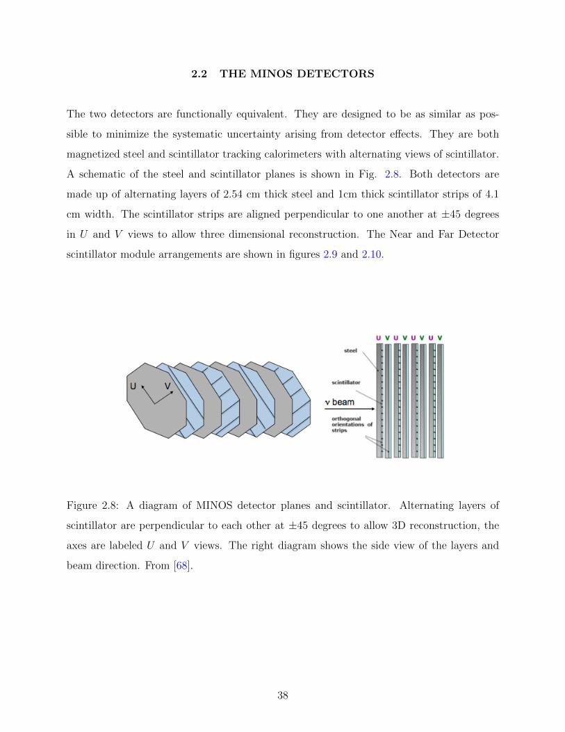
2.2 THE MINOS DETECTORS
The two detectors are functionally equivalent. They are designed to be as similar as pos-
sible to minimize the systematic uncertainty arising from detector effects. They are both
magnetized steel and scintillator tracking calorimeters with alternating views of scintillator.
A schematic of the steel and scintillator planes is shown in Fig. 2.8. Both detectors are
made up of alternating layers of 2.54 cm thick steel and 1cm thick scintillator strips of 4.1
cm width. The scintillator strips are aligned perpendicular to one another at ±45 degrees
in U and V views to allow three dimensional reconstruction. The Near and Far Detector
scintillator module arrangements are shown in figures 2.9 and 2.10.
Figure 2.8: A diagram of MINOS detector planes and scintillator. Alternating layers of
scintillator are perpendicular to each other at ±45 degrees to allow 3D reconstruction, the
axes are labeled U and V views. The right diagram shows the side view of the layers and
beam direction. From [68].
38
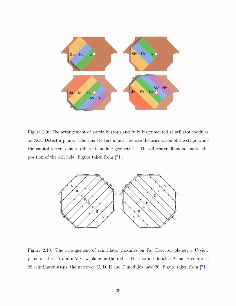
Figure 2.9: The arrangement of partially (top) and fully instrumented scintillator modules
on Near Detector planes. The small letters u and v denote the orientation of the strips while
the capital letters denote different module geometries. The off-center diamond marks the
position of the coil hole. Figure taken from [71].
Figure 2.10: The arrangement of scintillator modules on Far Detector planes, a U-view
plane on the left and a V-view plane on the right. The modules labeled A and B comprise
28 scintillator strips, the narrower C, D, E and F modules have 20. Figure taken from [71].
39

2.2.1 Near Detector
The Near Detector (ND), located 110 m underground at Fermilab, is a 4.8 m wide, 3.8 m
high squashed octagon with a length of 16.6 m. It consists of 282 steel planes and has a mass
of 980 tons. The first 120 planes are instrumented with scintillator, every fifth one fully and
the other four partially (see Fig. 2.9). The remainder of the detector has every fifth plane
fully covered with scintillator where intermediate four planes have no scintillator. See Fig.
2.11 for the cross section of a ND plane.
Figure 2.11: The cross section of a MINOS ND plane. The dark grey region indicates the
instrumented region of a partially instrumented plane. Fully instrumented planes have the
entire area covered with scintillator. The diamond in the center is the coil hole and the gray
dot on the left hand side denotes the center of the neutrino beam. From [69].
The upstream region of the detector is more finely instrumented and serves as the
calorimeter. The calorimeter is designed to measure hadronic showers while the partially
instrumented second half of the detector, the spectrometer, is for muon tracking. The de-
tector is magnetized to an average magnetic field strength of 1.3 T which focusing particles
40

of one charge sign and defocusing the other. The magnetic field allows the reconstruction of
the charge of a particle traveling through the detector; the curvature of a charged particle
is also used to reconstruct its momentum. The beam axis is horizontally approximately 1.5
m away from the coil in an attempt to minimize the number of tracks crossing the coil hole
region.
2.2.2 Far Detector
The Far Detector has an octagonal cross section 8m across, a length of 31 m and a mass
of 5.4 kton. It is made up of a total of 486 steel planes in two supermodules of 243 planes
each. The supermodules are separated by a gap of 1.2 m length. The event rate at the Far
Detector is of the order of a few events per day, in contrast to approximately ten interactions
per spill at the Near Detector. This is the reason for the detector’s larger size. It is deeper
underground than the Near Detector, at 2341 ft depth, to reduce the cosmic ray background.
Cosmic rays are also vetoed by a veto shield covering the top of the detector along its length.
The detector is uniformly instrumented where every plane has full coverage with 192 strips
of scintillator, except for the front planes of each supermodule. A magnetic coil runs down
the center and magnetizes the detector to an average magnetic field of 1.3 T strength, the
same as the Near Detector.
41

2.3 SCINTILLATOR
Each scintillator strip is made of polystyrene doped with scintillator fluors PPO and POPOP
and covered in a reflective coating of 85% polystyrene and 15% TiO2 by weight. A charged
particle traveling through the strip excites the fluor, which emits the absorbed energy in
ultra violet photons. Wavelength shifting (WLS) fibers, 1.2 mm in diameter, are embedded
in a 2 mm deep groove in the middle of each strip and run along the length of the strip.
See Fig. 2.12 for a schematic of the scintillator system. These WLS fibers absorb the UV
scintillation light and emit it in green (average wavelength of 530 nm) and transport it to
the end of the strip. The scintillator strips are grouped into modules of 13 to 28 strips and
enclosed in a 0.5 cm thick aluminum casing.
Figure 2.12: Cross sectional view of a MINOS scintillator strip, from [71].
42
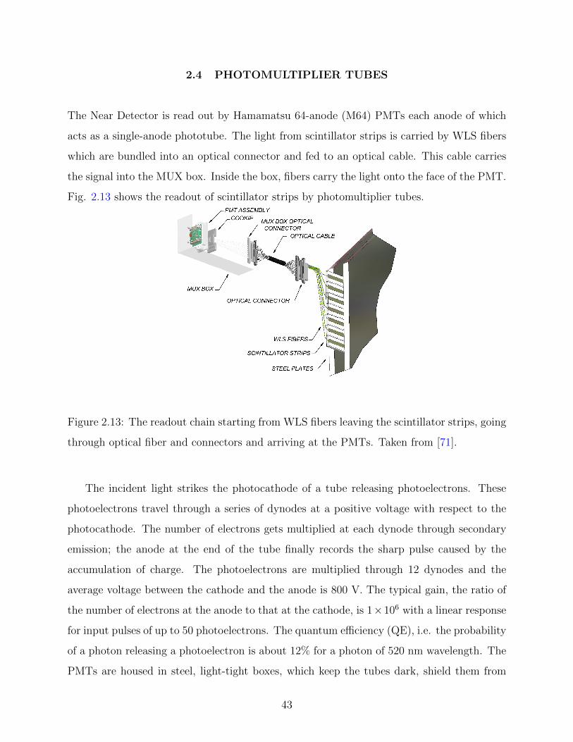
2.4 PHOTOMULTIPLIER TUBES
The Near Detector is read out by Hamamatsu 64-anode (M64) PMTs each anode of which
acts as a single-anode phototube. The light from scintillator strips is carried by WLS fibers
which are bundled into an optical connector and fed to an optical cable. This cable carries
the signal into the MUX box. Inside the box, fibers carry the light onto the face of the PMT.
Fig. 2.13 shows the readout of scintillator strips by photomultiplier tubes.
Figure 2.13: The readout chain starting from WLS fibers leaving the scintillator strips, going
through optical fiber and connectors and arriving at the PMTs. Taken from [71].
The incident light strikes the photocathode of a tube releasing photoelectrons. These
photoelectrons travel through a series of dynodes at a positive voltage with respect to the
photocathode. The number of electrons gets multiplied at each dynode through secondary
emission; the anode at the end of the tube finally records the sharp pulse caused by the
accumulation of charge. The photoelectrons are multiplied through 12 dynodes and the
average voltage between the cathode and the anode is 800 V. The typical gain, the ratio of
the number of electrons at the anode to that at the cathode, is 1×10⁶ with a linear response
for input pulses of up to 50 photoelectrons. The quantum efficiency (QE), i.e. the probability
of a photon releasing a photoelectron is about 12% for a photon of 520 nm wavelength. The
PMTs are housed in steel, light-tight boxes, which keep the tubes dark, shield them from
43

the magnetic field and shield the electronics from ambient electronic noise.
Each scintillator strip in the first 120 planes of the Near Detector, the calorimeter, is
read out individually: One strip connects to one PMT whose anode is read out by a unique
electronic channel. In the spectrometer there is 4:1 multiplexing, where four anodes are
connected in parallel and read out by one electronic channel in order to reduce the amount
of front-end electronics necessary. The four multiplexed strips are 1 m apart making the
muon tracking unambiguous.
In the Far Detector 16-anode Hamamatsu M16 PMTs are used. The multiplexing at the
Far Detector is such that eight fibers (from eight scintillator strips) are fed to one pixel in a
PMT. The strips from which these fibers carry light are at least one meter apart and result
in unambiguous track reconstruction. The Far Detector PMTs have gains of 1× 10⁶, linear
up to 100 photoelectrons and greater than 12% quantum efficiency.
A low pulse height hit (usually of less than one photoelectron) can be registered at a
nearest neighbor of an anode. This phenomenon is referred to as cross talk and is an artifact
of the multi-anode design of the phototubes; charge drifts from one anode to another. Total
cross talk in all pixels is 3.7% in Near Detector PMTs and 3.2% in Far Detector PMTs.
2.5 THE MAGNETIC FIELD
Both MINOS detectors are magnetized by a coil that passes through a hole cut through the
length of the detector. The Far Detector coil hole is at the center of the octagon and each
supermodule is magnetized independently by its own coil. The coil consists of 190 turns of
copper wire with Teflon insulation water-cooled by a copper jacket. Fig. 2.14 shows the
cross section of a Far Detector coil. An 80 A power supply gives a 15.2 kA-turn total current
providing an average toroidal magnetic field of 1.3 T strength [71]. One coil dissipates 20
kW of power.
In the Near Detector the coil hole is offset about 1.5 m to the right of the beam center so
that the fiducial volume excludes the coil hole region. This minimizes the number of tracks
that travel through the uninstrumented coil hole region and get reconstructed poorly. Due
44

Figure 2.14: Cross section of a Far Detector coil. The larger circles represent the copper
cooling tubes and the smaller circles are the 190 turns of copper wire. From [71].
to the squashed octagon geometry, a 40kA-turn current is required [71]. The ND coil, whose
conductor is made of aluminum, is also water-cooled and has eight turns. It dissipates a
power of 47 kW. The magnetic field in both detectors’ fiducial volumes are nearly uniform.
Field maps of both detectors can be seen in Fig. 2.15.
Figure 2.15: The left hand figure shows the Near Detector magnetic field map where off-
center diamond marks the position of the coil hole. On the right is the Far Detector field
map with the rectangular coil hole in the center. From [71].
45

2.6 ELECTRONICS AND DATA ACQUISITION
The Near and Far Detectors were designed to be as similar as possible to minimize the
effect of systematic uncertainties. The same electronics, however, could not be used for both
detectors. In the Far Detector the beam neutrino interaction rate is on the order of a few
per day, whereas the cosmic muon rate is around 0.5 Hz. By contrast, the Near Detector
sees on the order of 10 neutrino interaction events per every 10 µs spill. The following two
sections describe the Near and Far Detector front end electronics, followed by a section on
the data acquisition (DAQ) system which is common to the two detectors.
2.6.1 Near Detector Front-End Electronics
In order to resolve the amount of data it collects, Near Detector electronics are designed to
be fast and have no deadtime [71, 72]. The readout has a time resolution of 18.8 ns which
matches the 53 MHz frequency of the Main Injector RF cavities.
The signal from each PMT anode is fed into a QIE (Charge (Q) Current (I) Encoder),
which consists of a current splitter, gated integrator and range selector as shown in Fig.
2.16. The current is split into eight binary weighted ranges with values I/2, I/4, ..., I/256
and integrated onto a capacitor for each range. See Fig. 2.17 for a plot of the QIE response.
The capacitors are sensitive to their respective ranges. This saturates the capacitors of all
ranges below that corresponding to the signal size and the current in the first unsaturated
range provides a precision measurement of the signal. Splitting the current gives the QIE
chip sensitivity over a range of input charges, from 10 fC to 10 pC.
After integration, the voltage across the capacitors is fed to an ADC (analog/digital
converter) via a range selector. The voltage across one and only one of the capacitors is
within the predetermined limits of the ADC, which is selected by the range selector and
output to the ADC, along with a three bit number indicating the range value. The current
splitter integrates all the current in one clock cycle, selects the unsaturated range in the next
cycle. In the following clock cycle, the ADC converts the analog signal into an 8-bit digital
signal. A fourth cycle is required to reset the capacitors. In order to have deadtimeless
46

operation, there are four independent copies of the current splitter on the QIE. In addition
to the 8-bit ADC value and the 3-bit range value, a 2-bit code (called CAPID) identifies the
current splitter and capacitor from which the signal was read. This 13-bit output from the
ADC is stored on a FIFO (first in first out) buffer which can store digital signal from up to
1000 clock cycles (19 µs).
Figure 2.16: Block diagram of the QIE chip for the Near Detector. It has three main
components, current splitter, gated integrator and range selector. The chip digitizes the
analog signal from the PMT. From [72].
47

Figure 2.17: Response of the QIE chip. The x-axis shows the amount of charge injected into
the chip, the y-axis shows the ADC response for the different ranges. Only the first five of
the eight ranges are shown. From [71]
48
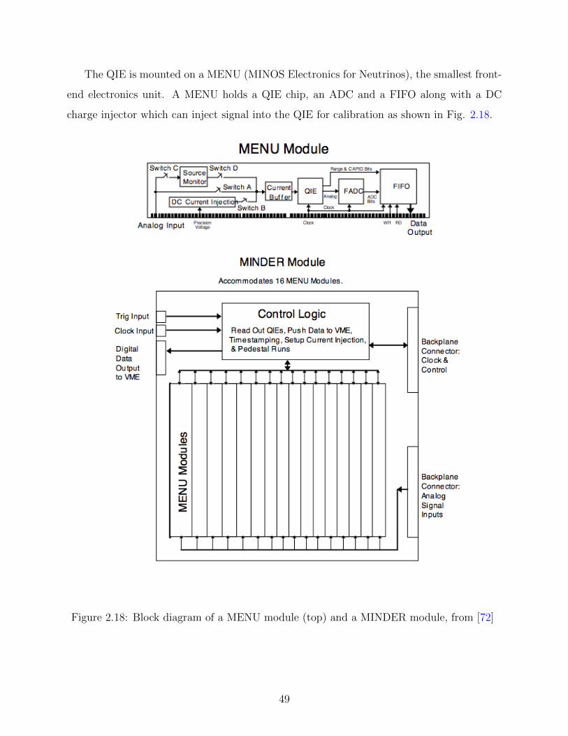
The QIE is mounted on a MENU (MINOS Electronics for Neutrinos), the smallest front-
end electronics unit. A MENU holds a QIE chip, an ADC and a FIFO along with a DC
charge injector which can inject signal into the QIE for calibration as shown in Fig. 2.18.
Figure 2.18: Block diagram of a MENU module (top) and a MINDER module, from [72]
49

Sixteen MENU boards are mounted on a MINDER module (MINOS Near Detector Elec-
tronics Readout, fig 2.18). The MINDER timestamps the signal and controls the power to
the MENUs. The MINDER reads all the output from its FIFOs and sends them to a single
FIFO on the MASTER module (MINOS Acquisition, Sparsifier and Time-stamper for Event
Readout). Eight MINDERS are connected to a MASTER which has two buffers, one is being
written to while the other is being read by a VME computer. The VME computers send
the data to the data acquisition system. The diagram in Fig. 2.19 provides a schematic
overview of the ND front-end electronics readout.
Figure 2.19: Overview of Near Detector front-end electronics, from [72]
50

2.6.2 Far Detector Front-End Electronics
The data rate at the Far Detector, 735 km downstream of the neutrino source and 700 m
underground, is much lower than that of the Near Detector: a few beam neutrino interactions
per day and a 0.5 Hz cosmic muon rate. This means electronics can be slower than the Near
Detector and deadtime can be tolerated. A diagram of the Far Detector front-end electronics
is presented in fig. 2.20.
Figure 2.20: Overview of the MINOS Far Detector readout electronics. Diagram from [71].
Each PMT is read out by a Viking VA chip using 17 of its 32 channels. 16 channels are
used to read out an anode each, and one channel reads out the PIN diode monitoring the
light injection system, see Sec. 3.2.1.1. The VA chips are mounted on VA front-end boards
(VFB) which provide power control and biasing for the VA chips. The VFB also houses a
chip called ADSLite. This chip receives a signal from the PMT and triggers the VA readout
if the signal is greater than 0.25 photoelectrons.
51
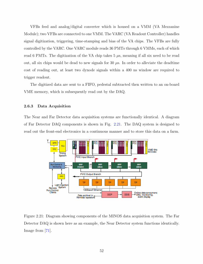
VFBs feed and analog/digital converter which is housed on a VMM (VA Mezzanine
Module); two VFBs are connected to one VMM. The VARC (VA Readout Controller) handles
signal digitization, triggering, time-stamping and bias of the VA chips. The VFBs are fully
controlled by the VARC. One VARC module reads 36 PMTs through 6 VMMs, each of which
read 6 PMTs. The digitization of the VA chip takes 5 µs, meaning if all six need to be read
out, all six chips would be dead to new signals for 30 µs. In order to alleviate the deadtime
cost of reading out, at least two dynode signals within a 400 ns window are required to
trigger readout.
The digitized data are sent to a FIFO, pedestal subtracted then written to an on-board
VME memory, which is subsequently read out by the DAQ.
2.6.3 Data Acquisition
The Near and Far Detector data acquisition systems are functionally identical. A diagram
of Far Detector DAQ components is shown in Fig. 2.21. The DAQ system is designed to
read out the front-end electronics in a continuous manner and to store this data on a farm.
Figure 2.21: Diagram showing components of the MINOS data acquisition system. The Far
Detector DAQ is shown here as an example, the Near Detector system functions identically.
Image from [71].
52
The DAQ reads out data continuously but only writes it to disk under certain conditions.
The Near Detector DAQ is triggered by the beam spill signal at Fermilab and all data
arriving within a 100 µs window around the spill is recorded. Since the Far Detector is not
at Fermilab, it cannot be triggered directly by the beam spill. Instead, it receives the GPS
timestamp of the beam spill from the Near Detector via the Internet.
A MASTER has two buffers, as discussed in section 2.6.1, one of which is being written
while the other is being read out, by a ROP (Readout Processor). The buffers are read
for the duration of one timeblock, 10-50 ms long. The ROP sends all the data collected
for one timeframe, 1 second in duration, to Branch Readout Processors (BRPs). The BRP
then sends this data to the trigger farm. The trigger farm constructs events from the raw
scintillator hit information and writes those that pass the triggering algorithm to disk. The
trigger farm is also responsible for storing calibration information.
2.7 CALIBRATION DETECTOR
The calibration detector, or CalDet, was a miniature but functionally equivalent model of
the MINOS Near and Far Detectors installed at CERN. It comprised 60 unmagnetized, steel
planes of 1 m2 area and 2.50 cm width. Planes were instrumented with 24 horizontal and 24
vertical scintillator strips. The strips were read out at one end by ND and at the other by FD
electronics to calibrate the differences in the two readout systems’ responses. Scintillation
light was carried by WLS fibers. In order to match MINOS ND and FD response, long fibers
were used: 6m clear fibers for one end and 3m for the other. Fig. 2.22 shows a subsection
of the calibration detector.
CalDet was placed in CERN PS (proton synchrotron) test beams consisting of electrons,
muons, pions and protons of momenta ranging between 0.2 and 10 GeV/c and collected data
between 2001-2003. Data was collected with varying settings multiple times to achieve a
run-to-run stability of better than 1% and corrected to remove systematic effects to better
than 2%. The resulting data was compared to Monte Carlo simulations of events using the
GEANT3 [73] simulation at both the Near and Far Detectors. Fig. 2.23 shows a comparison
53
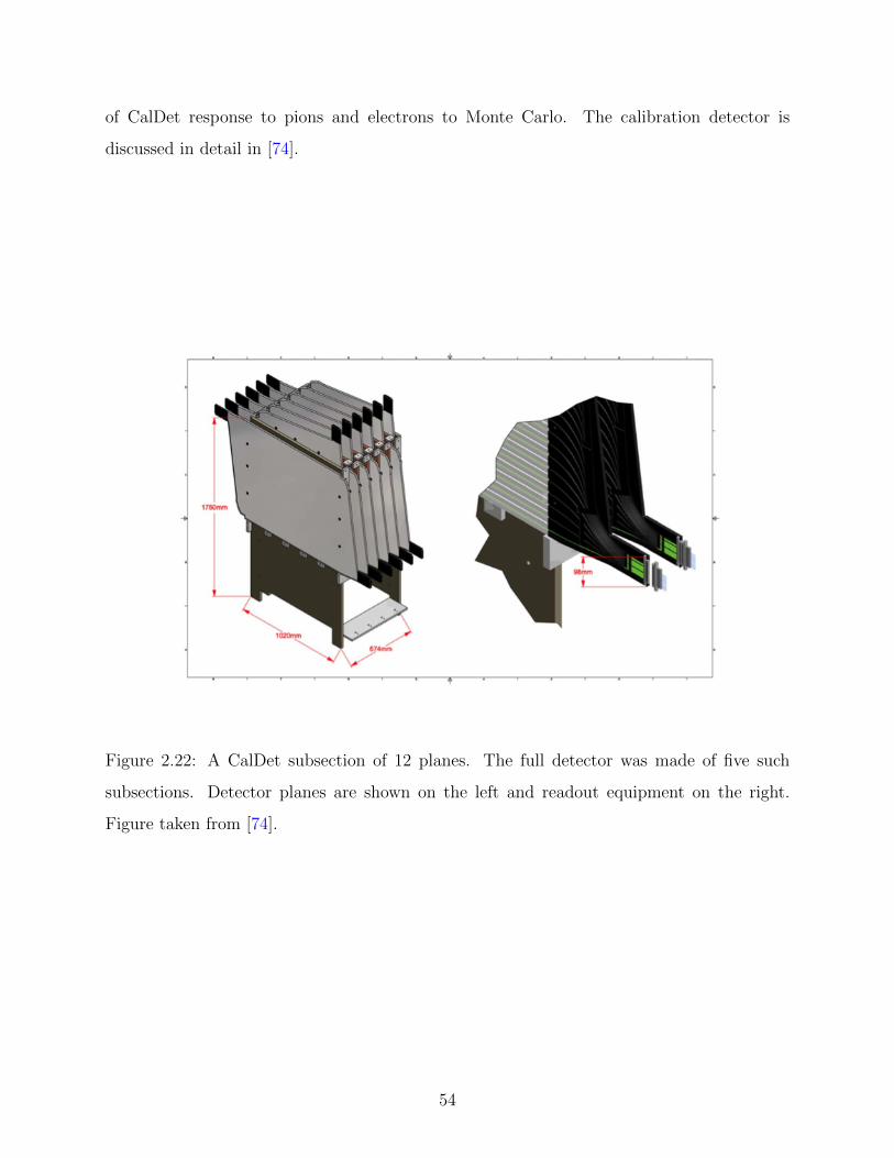
of CalDet response to pions and electrons to Monte Carlo. The calibration detector is
discussed in detail in [74].
Figure 2.22: A CalDet subsection of 12 planes. The full detector was made of five such
subsections. Detector planes are shown on the left and readout equipment on the right.
Figure taken from [74].
54
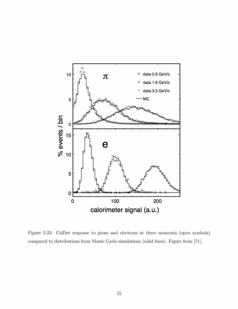
Figure 2.23: CalDet response to pions and electrons at three momenta (open symbols)
compared to distributions from Monte Carlo simulations (solid lines). Figure from [71].
55

2.8 NEAR AND FAR DETECTOR DIFFERENCES
Although ideally the two detectors would be perfectly identical, this is not possible in reality.
The event rate at the Near and Far detectors are vastly different because of the difference
in their proximity to the neutrino source. The ND rate is about 10 events per spill while
the FD sees a few beam neutrino interactions every day. Because of this, the FD is larger in
size. Scintillator strips at the FD are longer on average than the ND. FD strips are read out
at one end while ND strips are read out at both ends. Every FD plane is instrumented and
read out. The ND, on the other hand, is read out at every plane in the upstream calorimeter
region while only every fifth plane is instrumented in the downstream spectrometer half.
The FD coil hole is at the center of the detector while at the ND it is offset. This results
in small a difference in the magnetic fields. The fields are nearly identical inside the fiducial
volumes.
56
3.0 EVENT RECONSTRUCTION, CALIBRATION AND MONTE CARLO
SIMULATION
The reconstruction software uses the energy deposition (pulse height), topology and timing
of hits in the detector to identify neutrino interactions. The input to the reconstruction
chain is a snarl, the distribution of hits in the detector that arrive in one 10 µs spill. Fig.
3.1 shows a beam spill observed in the Near Detector. A snarl is divided into individual
slices based on the position and timing information of the hits. Tracks and showers are
constructed from slices which are then assembled into events. Physical event properties such
as position, vertex, length, angle and momentum of tracks, energy of showers are measured.
An event may have more than one track or shower but one of each is defined as the primary
track and shower. The event vertex is assigned as the first hit in the primary track. Section
3.1 details the steps of the reconstruction process.
Calibration, discussed in Section 3.2, aims to guarantee that the energy measurement
is accurate independent of time, in each strip of each detector and across the entire energy
range. It also corrects for the relative Near/Far detector differences. This is particularly im-
portant for the oscillation analyses which obtain the Far Detector prediction by extrapolating
the Near Detector data (see Sec. 4.7.
Processes in particle physics are probabilistic and event rates are low, especially for neu-
trino experiments. Simulations are needed to model physical processes and the experimental
apparatus.
57

3.1 RECONSTRUCTION
3.1.1 Slice Formation
Due to the high intensity of the neutrino beam, one snarl in the Near Detector contains
multiple neutrino interactions. Therefore, the first step in the reconstruction chain is dividing
the snarl into slices, which are clusters of hits localized in space and time. Calorimeter strips
with a charge deposition greater than two photoelectrons (pe), a time gap between two strips
of shorter than 20ns and a total time span of less than 300ns are formed into a slice. Slices
must contain at least two strips. If the slice thus formed has two strips with a spatial gap of
greater than 1m in the longitudinal direction, the slice is split into two, provided it doesn’t
span the coil hole. Calorimeter strips with a charge smaller than 2 pe and spectrometer
strips are added to the most suitable slice based on timing information.
In theory, Far Detector snarls are also sliced into multiple events, but the event rate at
the FD is so low that this is rarely necessary in practice. In fact, there are no events in most
snarls at the FD.
3.1.2 Track Reconstruction
Once slices are formed, the next link in the reconstruction chain is the application of a
track-finding algorithm. This algorithm uses a Hough transform [76] to find track segments
consisting of several hits aligned approximately linearly across several detector planes.
These segments are then added together to form a track candidate. This candidate track
is fit using a multi-pass Kalman Filter [77]. The filter works by moving up and down the
track estimating the state of the muon at each point along the track. It includes the effects of
noise and multiple scattering in its estimate as well as the expected curvature in the magnetic
field [75]. Based on this information the filter decides if a given hit should or should not be
part of the track. After two passes with the filter the track momentum, or more precisely,
charge-to-momentum ratio (q/p), is obtained from fitting the trajectory of the track. Other
track properties are also measured at this time in addition to the momentum, such as track
beginning and end positions in two views and the uncertainty in the charge/momentum
58

Figure 3.1: One snarl observed in the Near Detector. On the top left the beam’s-eye-view
of the spill where multiple events are distributed in position are shown. The top right
figure shows the distribution as a function of arrival time within one spill. The bottom
figure shows a reconstructed track in one detector view where gray vertical lines indicate
scintillator. Figure is taken from [75].
measurement. At 3 GeV the momentum measurement from curvature has a resolution of
11%.
59

If the track ends in the detector, a second, more accurate measurement of its momentum
is obtained from range. This measurement has a resolution of 4.6% and is used for all tracks
that do not exit the detector or end in the uninstrumented coil hole region. This task is
performed by the swimmer which swims a muon backwards along the track from the track
end to the beginning and sums the energy it should have lost in the steel and scintillator
using the GEANT3 simulation [73].
Muons with energies between 10 MeV and 10 GeV lose energy through ionization which
is described by the Bethe-Bloch equation and the energy loss in various media are tabulated
by Groom in [78]. CalDet (see Sec. 2.7) demonstrated the accuracy of the Bethe-Bloch
description, while the uncertainty in the agreement between data and simulation obtained
by incorporating the Groom tabulation into GEANT3 is 2%. This is taken as a systematic
uncertainty on the measurement from range. The curvature measurement for stopping tracks
is found to agree with the range measurement to within 1% which was conservatively added
linearly for a 3% uncertainty estimate on the curvature measurement.
3.1.3 Cluster Formation and Shower Reconstruction
Once the track is identified, the remaining hits localized in space and time are clustered to-
gether to construct the shower. Hits that are part of a track but have more energy than what
the muon would have deposited are added to the shower after the muon part is removed.
Only hits with an energy deposition of greater than two photoelectrons are considered since
the low pulse height region is difficult to model. Muon energies are reconstructed topolog-
ically but the detector granularity is too coarse to distinguish individual components of a
shower. There are two methods to measure the shower energy described below.
One method of measuring the shower energy is calorimetry where the energy of the shower
is calculated by summing the energy deposited by all of its constituent hits (after the energy
deposited in the steel is recovered). By this method, the hadronic shower energy resolution
is 56%/√E⊕
2% and the electromagnetic shower energy resolution is 21.4%/√E⊕
4%.
Another way of measuring shower energies is the k-nearest neighbors (kNN) method,
where shower energies are reconstructed by using the amount of deposited energy as well as
60

the spatial distribution of energy deposition in the shower. The method is presented in great
detail in [79] and summarized here.
For a D-dimensional kNN, D variables that are correlated with the shower energy con-
struct a D-dimensional space. The distribution of Monte Carlo events in this space are
known, since their true shower energies as well as the true values of the D variables are
known. The k nearest neighbors of the query event, whose shower energy is being estimated,
are found by computing its Euclidean distance to each of its neighbors and taking the k
closest ones. Let ~y be the query event we seek to identify and ~x the Monte Carlo event
whose true parameters are known. The squared distance between the two is given by
∆s2 =D∑i=1
(yi − xi)2
σ2i
, (3.1)
where σi is the standard deviation of the variable i. It is necessary to normalize the distance
by this standard deviation because the D input variables do not necessarily have the same
units, and if un-normalized the one with the widest numerical range would dominate.
For this estimator D = 3 variables were chosen:
• Calorimetric energy in the first two showers,
• total energy deposited within a 1m radius of the track vertex,
• number of planes in the primary shower.
The number of variables, D, and the number of neighbors, k were optimized to maximize
the sensitivity to oscillations [79]. Studies with varying the number of k neighbors yielded
that the optimal number of neighbors with maximum sensitivity for the size of the Monte
Carlo sample used was found to be k = 400. The shower energy is estimated separately for
Near and Far detector events using the corresponding Monte Carlo samples.
Ideally the reconstructed shower energy will be identical to the true energy. This is not
the case in reality, and the deviation of the ratio Ereco/Etrue from one is energy dependent;
below 5 GeV it goes up to 15%. To remedy this a 7th degree polynomial, energy dependent
correction is applied to the kNN shower energy estimate. The final estimate after the energy
correction improves the shower energy measurement across all energies with the greatest
61

improvement at low energy where the resolution is better than the calorimetric estimate by
up to 25%.
3.1.4 Event Formation
Events are formed by combining tracks and showers that are considered to be coming from
the same neutrino interaction based on a set of criteria. A track is associated with a shower
if the shower is within ±35 cm of the track location in both U and V views. If there is
no match satisfying this criteria then a number of tests are formed to determine showers
associated with a track [80]. Once all associations between reconstructed objects are found,
the next step is to build an event. In the most frequent and simplest case there is one track
and one shower in a slice which make up an event. In cases where there are multiple tracks or
showers, the track with the highest pulse height deposition (highest energy track) is selected
as the primary track. Additional tracks and showers are added to the event if they meet
various sets of association conditions with the existing components of the event; a logical
algorithm loops through all possible associations until the event includes all objects that are
believed to belong to it. If there is no track, the initial seed is a shower and its associated
showers are added to the event in a similar fashion.
3.2 CALIBRATION
A light injection system is used to measure the linearity and time variation of PMTs and
electronics response, and cosmic ray muons are used to measure variations in scintillator
strip light output with time and position. No sources of known-energy particles are available
to the Near and Far Detectors, but data from the calibration detector (Sec. 2.7) provides
measurements to determine the relative and absolute energy scales of both detectors.
Calibration is a multi-stage process that converts the raw pulse height, Qraw, to the fully
corrected signal, Qcorr via a multiplicative calibration constant at each stage, Eq. 3.2. The
pulse height and calibration constants are functions of the scintillator strip, s, position, x,
62

time, t and detector, d.
Qcorr = Qraw(s, x, t, d)×DPMT(d, t)× L(d, s,Qraw)
×Dscint(d, t)× S(s, d, t)× A(d, s, x)×M(d) (3.2)
where D is the drift correction that accounts for changes in scintillator, PMT and electronics
response with temperature and time; L linearizes the response of each channel; S removes
differences from strip to strip; A corrects for attenuation depending on the position of the
hit in the strip, and M is the energy scale factor that corrects the pulse height to the same
energy unit in both detectors.
3.2.1 Calibration Procedure
3.2.1.1 PMT and Electronics Drift DPMT(d, t) The light injection (LI) system [81,
82] is designed to monitor and compensate for changes in the PMT gains and non-linearity.
It uses light-emitting diodes (LEDs) to inject ultraviolet light into the wavelength shifting
fibers, simulating scintillator light. 20 LEDs are housed in a pulser box and illuminate
multiple individual fibers. The intensity of injected light is monitored by PIN diodes while
simultaneously read out by PMTs. The LI system pulses periodically at the end of every
strip: 300 times per hour at the FD and 1000 times per hour at the ND. This is designed
to average 50 photoelectrons per pulse per PMT pixel in both detectors. Changes in LED
intensity can lead to variations of up to a factor of two in this light level; such changes are
monitored and corrected.
This LI data is collected once a month at each detector. PMT gains are measured using
photon statistics [81]. Gains measured by the LI system provide corrections to the PMT
gain and electronics response. Short term variations that are usually due to temperature
variations can be eliminated by good environmental control, while longer term variations
due to aging and changes in hardware amount to ∼ 4%/year.
63
3.2.1.2 Linearity L(d, s,Qraw) PMT and electronics responses are not linear for light
levels greater than approximately 100 photoelectrons. The LI system is utilized to correct for
this nonlinearity by injecting a known intensity of light into scintillator strips, ranging from
a few to hundreds of photoelectrons, and measuring the electronics response as a function
of true illumination. In the Near Detector, the charge integration and ADC electronics are
also calibrated for linearity by directly injecting charge into the front-end electronics
3.2.1.3 Scintillator Drift Correction Dscint(d, t) The scintillator response changes
in time as the material ages. Aging reduces the light level by about 2% annually and
environmental variations, mainly temperature, result in short-term changes. The response
of the detectors is measured by monitoring the median response of a detector plane to
through-going cosmic muons. Although the spectra of cosmic muons are different between
detectors, due to differences in depth, zenith angle and latitude, the energy spectra and rate
of cosmic muons going through one detector is time independent. It is therefore possible to
calibrate for this drift by comparing the median detector response at time t to the response
at time t0, the beginning of the experiment:
Dscint(d, t) =Median response (d, t0)
Median response (d, t)(3.3)
3.2.1.4 Strip-to-strip Calibration S(s, d, t) The strip-to-strip non-uniformity cor-
rection accounts for several detector effects including scintillator light yield, WLS collection
efficiency, differences in attenuation optical fibers, PMT quantum efficiency and PMT gain.
The correction is obtained by using cosmic ray muons in the minimum ionizing energy range
(a few GeV), since these muons’ energy deposition is relatively independent of their mo-
menta. An individual strip’s response is characterized by constructing the muon spectrum
for that strip from cosmic ray muon data accumulated over a period of time. The calibration
constant is then calculated monthly as the strip response normalized by the mean response
of all strips:
S(s, d, t) =Mean response of whole detector (d, t)
Response of strip (s, d, t)(3.4)
64

3.2.1.5 Attenuation A(d, s, x) The response of one strip can show variations between
different transverse positions on the strip mainly because of WLS attenuation. The calibra-
tion constant is given by,
A(d, s, x) = Ad,s1 e−x/Ld,s1 + Ad,s2 e−x/L
d,s2 (3.5)
where x is the transverse position along the strip and Ld,s1 and Ld,s2 are the attenuation lengths.
This correction was calculated by using a module mapper. The module mapper measured
the response of each scintillator module to ionizing radiation using a 137Cs source. To obtain
the calibration constant, i.e., the values of A1, A2, L1 and L2, a fit is performed for each strip
and resulting parameters are used to correct the data [71]. The attenuation correction was
later cross checked by using through-going muons and was found to be consistent to within
4% [68].
3.2.1.6 Inter-detector Calibration M(d) In addition to correcting each of the three
detectors’ responses to be spatially and temporally consistent within one detector, the calori-
metric responses of the Near and Far Detectors and CalDet are calibrated to normalize the
energy scales of the three detectors. This calibration is performed by using the stopping
cosmic ray muons sample. Stopping cosmic muons make up a small fraction of the total
cosmic sample (∼ 0.3% at the FD) but there are enough cosmic rays that stopped muons
are a sufficient dataset for this purpose. Stopping muons are used because their energy
depositions are well understood, especially between 0.5 GeV and 1.1 GeV where their dEdx
is
nearly constant. Because of this, the track window technique is used, where the end 0− 0.5
GeV portion of the track is discarded. The detectors’ energy scales are normalized to within
the target of 2% using this method [71]. To be able to compare the response of the ND, FD
and CalDet a unit of muon energy equivalent (MEU) is defined as the detector response to
a perpendicular minimum ionizing particle in the energy range 0.5− 1.1 GeV traversing one
scintillator plane. To determine the constant relating the measured signal to actual energy
loss, CalDet data that lie in the track window were fit to the Bethe-Bloch equation, which
governs the energy loss of a muon by ionization.
65
3.2.2 Absolute Energy Scale
The absolute track and shower energies were determined using data collected by CalDet while
it was exposed to various test beams of known composition and energy at CERN. CalDet
collected data with pions, protons, electrons and muons of both positive and negative charge
signs in the energy range 200 MeV to 10 GeV while other detectors in the beamline were
utilized to identify the particles. The range of stopping muons (of momenta smaller than 2.2
GeV/c) was modeled to better than 3% accuracy with GEANT3, while the detector response
to electrons was simulated with an accuracy better than 2%. The pion and proton induced
showers were reproduced to better than 6% accuracy with the GCALOR [83] simulation.
3.3 MONTE CARLO SIMULATION
Monte Carlo models interactions by repeatedly simulating each neutrino interaction and final
state particle, which has a probability density function (PDF), a large number of times so
that the available phase space is sufficiently sampled. To construct a reliable simulation,
each component of the physical processes and the experiment need to be modeled. For
MINOS, these can be broken down into two steps: the simulation of the neutrino flux, and
the simulation of interactions of these neutrinos with detectors.
The flux simulation relies on the FLUGG [68] package, which combines the FLUKA [84,
85] software for particle interactions and propagation with the GEANT4 [86, 87] geometry
package. The flux simulation models hadron production at the target, focusing by horns,
and subsequent decays which produce neutrinos in the decay pipe. The FLUGG package
is able to model the beamline with a detailed description of the target position (including
a 1 cm shift for part of the datataking period) and the effects of helium in the decay pipe
for run periods after November 2007. The flux is simulated separately for each run period
to account for these effects accurately. The results of the simulation are “flux files” that
contain details of hadrons, muons and the daughter neutrinos from their decays.
For the second step of the simulation, the NEUGEN3 [88] neutrino interaction generator
66

software simulates neutrino interactions by using the above flux files as input. NEUGEN
simulates both the neutrino interaction in the detector and the reinteraction of final state
hadrons with nuclear matter. Interactions in the surrounding area and rock are simulated
and overlaid with the detector interactions. The effect of multiple interactions in the same
spill are also taken into account by overlaying individual simulated events [89] at this stage.
Once neutrino interactions are generated, GMINOS [90] simulates the propagation of
particles through the detector. The modeling of the propagation is energy dependent and
the simulation includes a detailed model of the detector geometry from GEANT3. Hadronic
showers are modeled by the GCALOR [83] software chosen for its good agreement with data
from the calibration detector (see Sec. 2.7). This part of the simulation outputs energy
deposition in the detector.
This resulting energy deposition is converted into light and taken through the WLS fiber
to the PMT cathode where it is converted to photoelectrons by the MINOS package Pho-
tonTransport. Another MINOS package, DetSim, simulates the next steps: photomultiplier
tubes and readout electronics. Detailed information about PMTs and electronics’ behavior
is included in the simulation, such as cross-talk, non-linearity, and noise.
To best represent real interactions, the simulated energy deposition signal is uncalibrated
by applying the calibrations described in section 3.2 in reverse before conversion to light.
In order to determine which calibration constants to use, the simulated data is assigned a
random date from the pool of dates when actual data was collected so that data and Monte
Carlo have the same distribution of calibration constants. This fake date is recorded and
when Monte Carlo is calibrated the appropriate constants are used.
The effect of neutrino oscillations in Monte Carlo is taken into account during analysis
by reweighting the events and by using special “tau files.” These tau files contain events in
a scenario where the oscillation probability P (νµ → ντ ) = 1, whereas the standard Monte
Carlo is unoscillated with P (νµ → νµ) = 1. Then the spectra in any oscillation scenario can
be constructed by an appropriate linear combination of the standard Monte Carlo and these
tau files.
67
4.0 ANTINEUTRINO OSCILLATION ANALYSIS
To measure antineutrino oscillation parameters the Far Detector observed event rate as a
function of energy is compared with prediction. We fit for the mixing angle and mass splitting
between the second and third mass states in the two-flavor oscillation model explained in
Section 1.3.
The data used to measure antineutrino oscillations was collected between 2009 and 2011
during two run periods in reversed horn current (RHC) mode. MINOS quantifies the amount
of data in units of protons-on-target (POT): the number of protons striking the graphite tar-
get. A total of 2.95×10²⁰ POT antineutrino-mode data was analyzed to measure antineutrino
oscillations. This chapter details the steps of the analysis and presents the results.
4.1 EVENT TOPOLOGIES
There are multiple event topologies in the MINOS detectors. Charged-current νµ and νµ
interactions leave a µ− and µ+ in the detector respectively. The muon energy deposition
pattern produces a long track that curve in the magnetic field. In neutrino-mode running,
the toroidal field curves a µ− towards the coil hole and µ+ away. Events curving towards the
coil hole are more likely to be contained allowing their energy to be measured from range
which is more accurate than the measurement by curvature. Exiting events’ momenta are
measured from curvature. In antineutrino-mode the detector field is reversed and µ+ tracks
are focused.
NC and CC νe interactions produce events without tracks or with very short tracks.
They are characterized by showers. NC showers are more diffuse while CC νe showers have
68
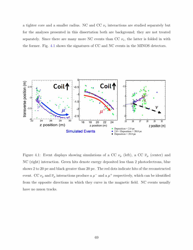
a tighter core and a smaller radius. NC and CC νe interactions are studied separately but
for the analyses presented in this dissertation both are background; they are not treated
separately. Since there are many more NC events than CC νe, the latter is folded in with
the former. Fig. 4.1 shows the signatures of CC and NC events in the MINOS detectors.
Figure 4.1: Event displays showing simulations of a CC νµ (left), a CC νµ (center) and
NC (right) interaction. Green hits denote energy deposited less than 2 photoelectrons, blue
shows 2 to 20 pe and black greater than 20 pe. The red dots indicate hits of the reconstructed
event. CC νµ and νµ interactions produce a µ− and a µ+ respectively, which can be identified
from the opposite directions in which they curve in the magnetic field. NC events usually
have no muon tracks.
69
4.2 EVENT SELECTION
Near and Far detector data samples are obtained by requiring that events meet a series of
selection criteria. The pre-selection common to both detectors ensures data quality. Each
detector has its own fiducial volume requirements. The analysis selection is designed to
separate positively and negatively charged final state muons and separates charged current
νµinteractions from neutral currents.
4.2.1 Pre-selection
Before analysis-specific event selection, all events need to meet a set of data quality criteria.
It is required that NuMI is operating in the low-energy mode (see Fig. 2.7) for which the
target sits inside the first horn, the separation between the two horns is 10.0 m and the horn
current is set to 185 kA. The direction of the horn current in antineutrino mode is such that
it focuses negatively charged mesons and deflects positively charged ones. Both detector
coils need to be on so that the detectors are magnetized. In antineutrino-mode the coil
current is ’reversed’ to focus positively charged particles towards the coil hole. For an event
to be included in the data sample it must arrive within a beam spill so that atmospheric
and cosmic background is reduced. Events are required to be reconstructed with at least
one muon track, since all events relevant to this analysis are charged-current interactions
with a muon in the final state. Track vertices are required to lie within the respective
fiducial volumes of the detectors; this requirement aims to guarantee that all events have
their hadronic shower fully contained inside the detector.
4.2.2 Far Detector Fiducial Volume
The event rate at the Far Detector is low (a few neutrino interactions per day) and it is
essential to record and keep as many events as possible to maximize the statistical power of
the analysis. The FD fiducial volume is therefore chosen to be as large as possible. FD events
must be inside a radius range of 40 cm < R <√
14 m. The inner limit excludes events too
close to the un-instrumented magnetic coil region where reconstruction is not well modeled.
70
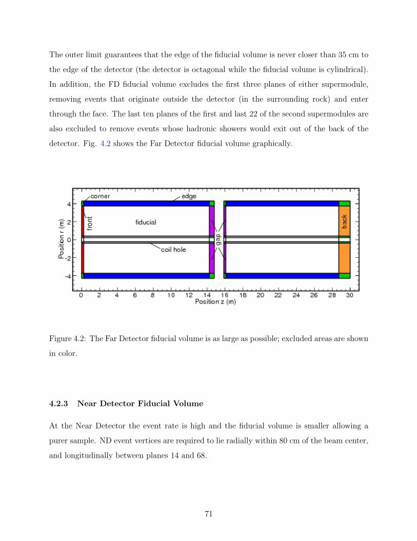
The outer limit guarantees that the edge of the fiducial volume is never closer than 35 cm to
the edge of the detector (the detector is octagonal while the fiducial volume is cylindrical).
In addition, the FD fiducial volume excludes the first three planes of either supermodule,
removing events that originate outside the detector (in the surrounding rock) and enter
through the face. The last ten planes of the first and last 22 of the second supermodules are
also excluded to remove events whose hadronic showers would exit out of the back of the
detector. Fig. 4.2 shows the Far Detector fiducial volume graphically.
Figure 4.2: The Far Detector fiducial volume is as large as possible; excluded areas are shown
in color.
4.2.3 Near Detector Fiducial Volume
At the Near Detector the event rate is high and the fiducial volume is smaller allowing a
purer sample. ND event vertices are required to lie radially within 80 cm of the beam center,
and longitudinally between planes 14 and 68.
71

4.2.4 Separation of charged-current and neutral-current events
Fig. 4.1 shows the signatures of the two main kinds of muon neutrino interactions in the
MINOS detectors: charged-current (CC) and neutral-current (NC). CC antineutrino inter-
actions (middle panel) are the signal we need to extract for this analysis and the first step
is to distinguish charged and neutral current interactions.
In order to do this an algorithm called k-Nearest Neighbors (kNN) is employed. This
is a multivariate method in which an N-dimensional space of track variables is constructed.
A query event is identified as signal-like (CC) or background-like (NC) by its k neighbors’
characteristics. The distance in kNN space is determined by
D =
(d∑i=1
∣∣∣XMCi −XQ
i
∣∣∣2)12
(4.1)
where ~X is a vector in kNN multivariate space with MC denoting the Monte Carlo events of
known type (charged or neutral current) and Q denoting the query event. The probability
that the query events is a signal event is then given by the particle identification parameter
(kNN PID) is then given by
kNNID =kS
kS + kB(4.2)
where S and B denote signal and background respectively. In the cartoon in Fig. 4.3, red
dots denote signal and blue dots background. In this case k = 12, kS = 8, kB = 4 which
gives the query event marked by the star a kNNID of 23.
In general the N variables which make up the kNN space have different units. The
variables need to be normalized in order to avoid an arbitrary bias resulting in some of the
variables having larger weight in the overall discrimination power (i.e. an ellipse containing
a different set of events instead of the circle in the cartoon in Fig. 4.3). The normalization
scale factor for each variable is determined to be the width of its distribution.
The kNN space in this analysis is constructed by four variables that can distinguish
between charged and neutral current events (shown in Fig. 4.5) and uses k = 80 neighbors.
The first two variables quantify the topology of the track and the other two describe the
72

Figure 4.3: A cartoon demonstrating the use of the kNN particle identification in two-
dimensional kNN space. 12 nearest neighbors lie in the dashed circle, red representing signal
and blue representing background. This gives the event a kNN PID value of 23.
energy deposition along the track. The value of k was optimized such that the k neighbors
represent the local behavior of the probability density functions with little fluctuation in the
classification outcome. The development and use of the kNN algorithm is discussed in great
detail in [91].
• Number of scintillator planes in track. The number of planes that a muon pene-
trates is a direct measure of the length of the track. Muons can travel a long distance
through matter unlike hadrons which shower, so long tracks are easily identified as muons.
• Transverse track profile. A scintillator plane is made of closely packed scintillator
planes (see Fig. 2.8). A typical muon track deposits energy in one scintillator strip per
plane, whereas a hadronic shower has a wider transverse profile that spreads out to a
few planes. The transverse track profile parameter is computed by taking the ratio of
the number of track hits to the total number of hits within a small window of space and
time around the track, away from the vertex.
73
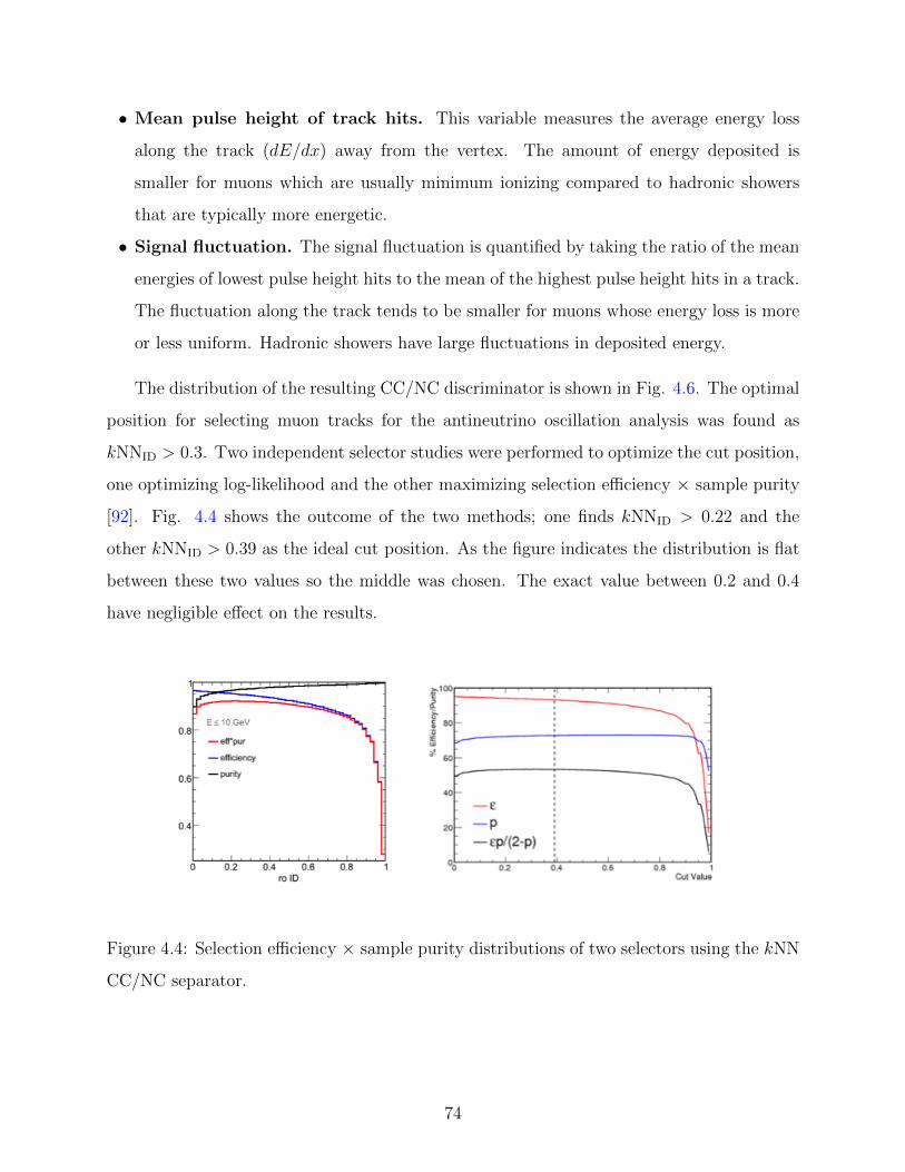
• Mean pulse height of track hits. This variable measures the average energy loss
along the track (dE/dx) away from the vertex. The amount of energy deposited is
smaller for muons which are usually minimum ionizing compared to hadronic showers
that are typically more energetic.
• Signal fluctuation. The signal fluctuation is quantified by taking the ratio of the mean
energies of lowest pulse height hits to the mean of the highest pulse height hits in a track.
The fluctuation along the track tends to be smaller for muons whose energy loss is more
or less uniform. Hadronic showers have large fluctuations in deposited energy.
The distribution of the resulting CC/NC discriminator is shown in Fig. 4.6. The optimal
position for selecting muon tracks for the antineutrino oscillation analysis was found as
kNNID > 0.3. Two independent selector studies were performed to optimize the cut position,
one optimizing log-likelihood and the other maximizing selection efficiency × sample purity
[92]. Fig. 4.4 shows the outcome of the two methods; one finds kNNID > 0.22 and the
other kNNID > 0.39 as the ideal cut position. As the figure indicates the distribution is flat
between these two values so the middle was chosen. The exact value between 0.2 and 0.4
have negligible effect on the results.
Figure 4.4: Selection efficiency × sample purity distributions of two selectors using the kNN
CC/NC separator.
74

Figure 4.5: Distributions of the four kNN input variables before CC/NC selection is applied.
The red histogram represents charged current Monte Carlo events, blue shows neutral cur-
rents, and black dots show data. The distributions of CC and NC events are significantly
different in each variable making it possible to separate the two.
75
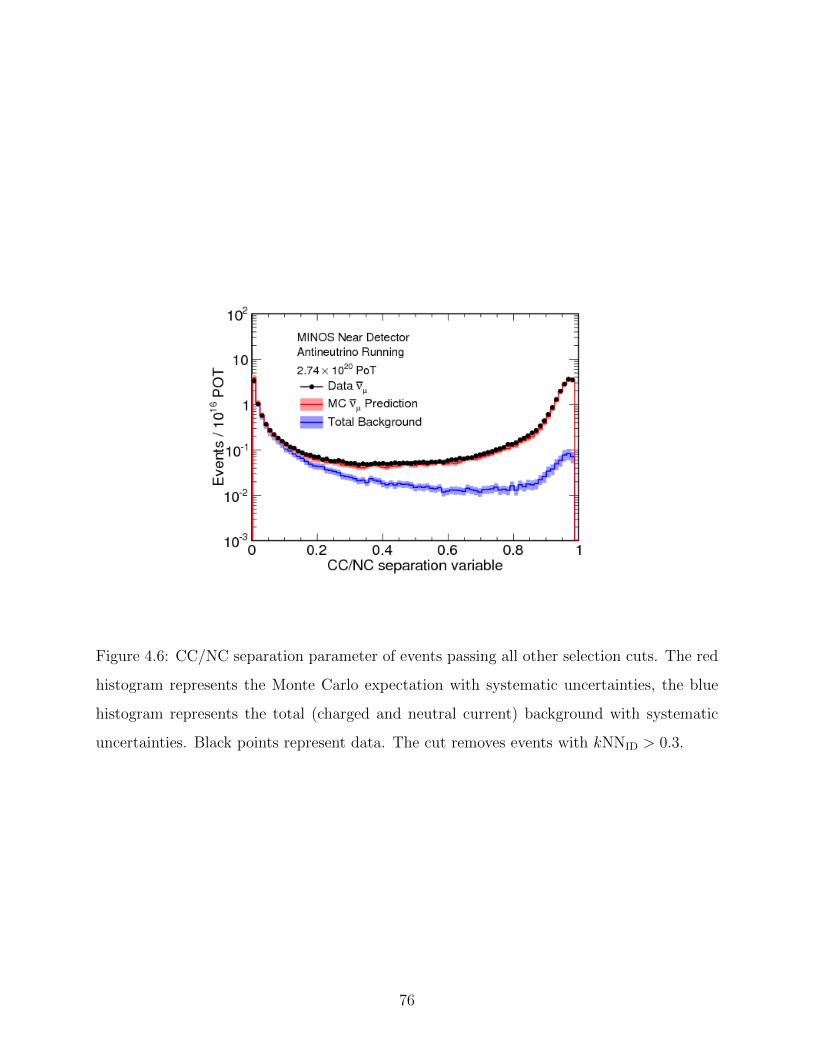
Figure 4.6: CC/NC separation parameter of events passing all other selection cuts. The red
histogram represents the Monte Carlo expectation with systematic uncertainties, the blue
histogram represents the total (charged and neutral current) background with systematic
uncertainties. Black points represent data. The cut removes events with kNNID > 0.3.
76
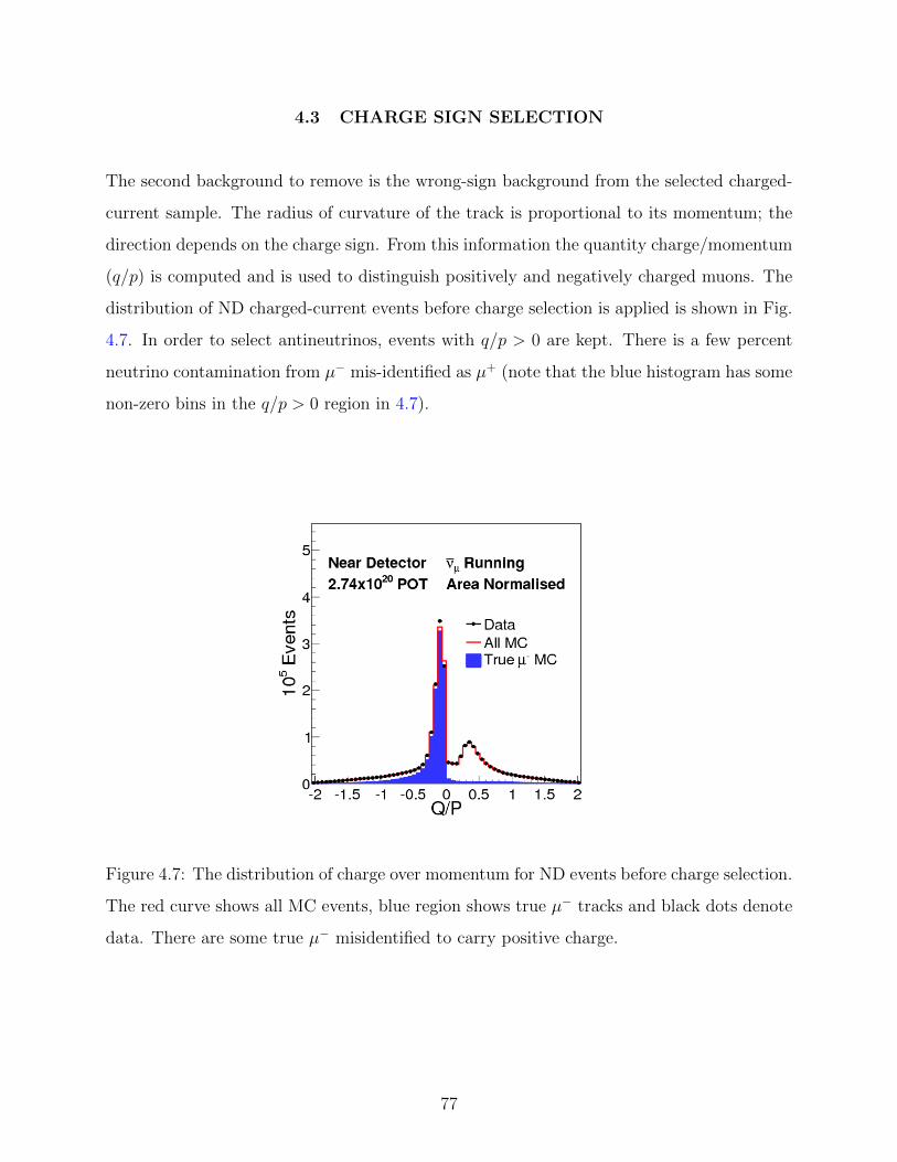
4.3 CHARGE SIGN SELECTION
The second background to remove is the wrong-sign background from the selected charged-
current sample. The radius of curvature of the track is proportional to its momentum; the
direction depends on the charge sign. From this information the quantity charge/momentum
(q/p) is computed and is used to distinguish positively and negatively charged muons. The
distribution of ND charged-current events before charge selection is applied is shown in Fig.
4.7. In order to select antineutrinos, events with q/p > 0 are kept. There is a few percent
neutrino contamination from µ− mis-identified as µ+ (note that the blue histogram has some
non-zero bins in the q/p > 0 region in 4.7).
Figure 4.7: The distribution of charge over momentum for ND events before charge selection.
The red curve shows all MC events, blue region shows true µ− tracks and black dots denote
data. There are some true µ− misidentified to carry positive charge.
77
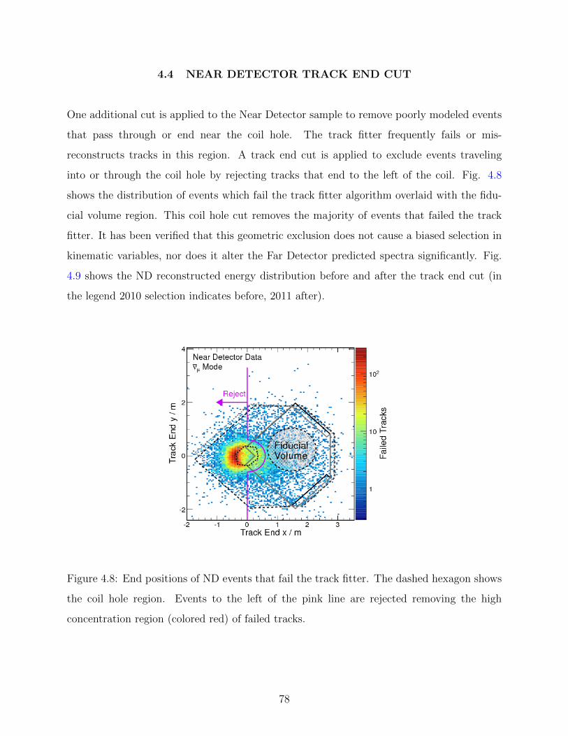
4.4 NEAR DETECTOR TRACK END CUT
One additional cut is applied to the Near Detector sample to remove poorly modeled events
that pass through or end near the coil hole. The track fitter frequently fails or mis-
reconstructs tracks in this region. A track end cut is applied to exclude events traveling
into or through the coil hole by rejecting tracks that end to the left of the coil. Fig. 4.8
shows the distribution of events which fail the track fitter algorithm overlaid with the fidu-
cial volume region. This coil hole cut removes the majority of events that failed the track
fitter. It has been verified that this geometric exclusion does not cause a biased selection in
kinematic variables, nor does it alter the Far Detector predicted spectra significantly. Fig.
4.9 shows the ND reconstructed energy distribution before and after the track end cut (in
the legend 2010 selection indicates before, 2011 after).
Figure 4.8: End positions of ND events that fail the track fitter. The dashed hexagon shows
the coil hole region. Events to the left of the pink line are rejected removing the high
concentration region (colored red) of failed tracks.
78

Figure 4.9: The reconstructed antineutrino energy distribution at the Near Detector with
(black) and without (red) the track end cut. The bottom plot shows the ratio of the spectrum
with the cut to the one without.
4.5 BEAM TUNING
The accuracy of the simulation of neutrino interactions in the detector depends on the
accuracy of the simulation of the flux of neutrinos going through the detector, which in turn
depends on the knowledge of production of pions and kaons in the target and of the focusing
optics. Uncertainties in the hadron production model generate significant uncertainties in
the overall neutrino flux prediction.
The built in flexibility of NuMI allowed data collection in multiple beam configurations
(see Fig. 2.7). By simulating the flux in these various beam configurations and performing a
multi-variable fit, the flux prediction was tuned to achieve good agreement with the observed
Near Detector data. The fit constrains the π+/π− ratio by using both simulated results from
79

FLUKA05 and experimental results from the NA49 experiment [93]. It is a simultaneous fit
across all beam configurations and separate runs. The best fit is used to determine a weight
for the pion (and kaon) which is propagated to the Near and Far detectors.
The hadron production is parametrized following the BMPT parametrization, [94],
d2N
dxFdpT= [A+BpT ] · exp
(−C3/2pT
)(4.3)
where pT is the transverse momentum of the meson and xF = pZ/pproton is the ratio of its
longitudinal momentum to the momentum of the proton. Parameters A(xF ), B(xF ), C(xF ),
which are functions of xF , are obtained by fitting with functions of xF . A, B, C are redefined
for π+ as,
A′(xF ) = (par[0] + par[1] · xF ) · A(xF )
B′(xF ) = (par[2] + par[3] · xF ) ·B(xF )
C ′(xF ) = (par[4] + par[5] · xF ) · C(xF ) (4.4)
and similarly for K+ with parameters par[6] through par[11]. The weight of a meson is
calculated as
W (π+/K+, pT , pZ) =[A′ +B′pT ] · exp
(−C ′3/2pT
)[A+BpT ] · exp (−C3/2pT )
(4.5)
Two additional parameters are needed to define the conversion between π+ and π−
weights; two more to do the same for K+ to K−. This brings the total number of hadron
production fit parameters to sixteen. There are a further eight parameters in the fit to
account for uncertainties in the flux measured by the Near Detector such as focusing, detector
effects and target degradation. The effect of the fit on can be seen in Fig. 4.10 where the
improvement of the agreement between data and Monte Carlo is apparent. The tuning
was designed to be used with neutrino-mode beam configurations, and adapted to provide
appropriate weights for antineutrino-mode Monte Carlo Fig. 4.11 shows comparisons of ND
data to tuned and untuned MC in and antineutrino modes.
80

Figure 4.10: Data (black dots), untuned (blue) and tuned (red) Monte Carlo comparison of
the Near Detector neutrino energy spectrum. The tuning significantly improves the agree-
ment between data and simulation.
81
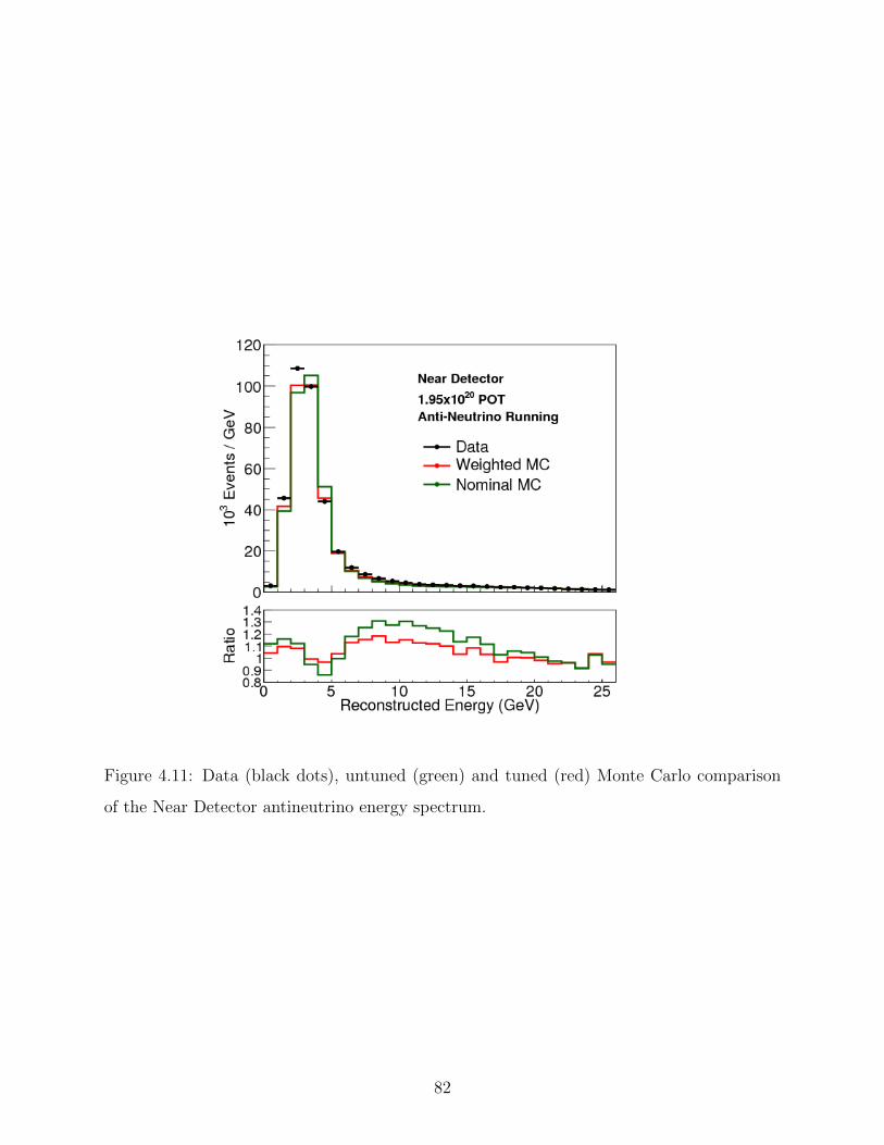
Figure 4.11: Data (black dots), untuned (green) and tuned (red) Monte Carlo comparison
of the Near Detector antineutrino energy spectrum.
82
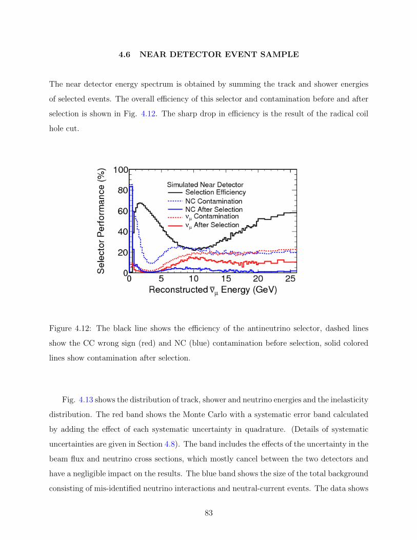
4.6 NEAR DETECTOR EVENT SAMPLE
The near detector energy spectrum is obtained by summing the track and shower energies
of selected events. The overall efficiency of this selector and contamination before and after
selection is shown in Fig. 4.12. The sharp drop in efficiency is the result of the radical coil
hole cut.
Figure 4.12: The black line shows the efficiency of the antineutrino selector, dashed lines
show the CC wrong sign (red) and NC (blue) contamination before selection, solid colored
lines show contamination after selection.
Fig. 4.13 shows the distribution of track, shower and neutrino energies and the inelasticity
distribution. The red band shows the Monte Carlo with a systematic error band calculated
by adding the effect of each systematic uncertainty in quadrature. (Details of systematic
uncertainties are given in Section 4.8). The band includes the effects of the uncertainty in the
beam flux and neutrino cross sections, which mostly cancel between the two detectors and
have a negligible impact on the results. The blue band shows the size of the total background
consisting of mis-identified neutrino interactions and neutral-current events. The data shows
83

good agreement with Monte Carlo and the disagreements are within limits of the systematic
error.
Figure 4.13: Plots show the distributions of track, shower and total antineutrino energy and
inelasticity. Black dots represent ND data, red curve represents Monte Carlo where the pink
band is the systematic error. The blue band shows the total background of neutral current
and wrong-sign events.
84
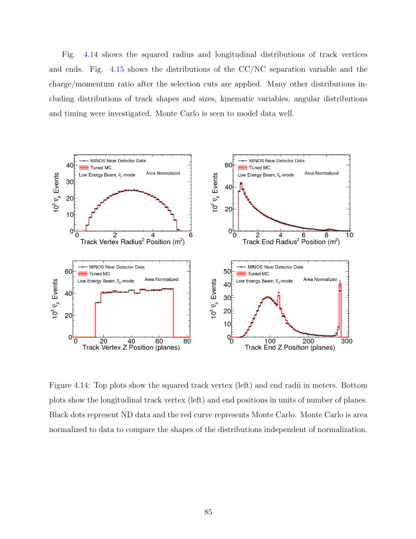
Fig. 4.14 shows the squared radius and longitudinal distributions of track vertices
and ends. Fig. 4.15 shows the distributions of the CC/NC separation variable and the
charge/momentum ratio after the selection cuts are applied. Many other distributions in-
cluding distributions of track shapes and sizes, kinematic variables, angular distributions
and timing were investigated. Monte Carlo is seen to model data well.
Figure 4.14: Top plots show the squared track vertex (left) and end radii in meters. Bottom
plots show the longitudinal track vertex (left) and end positions in units of number of planes.
Black dots represent ND data and the red curve represents Monte Carlo. Monte Carlo is area
normalized to data to compare the shapes of the distributions independent of normalization.
85

Figure 4.15: The top plot shows CC/NC separation parameter of events passing all se-
lection cuts. The bottom shows the charge/momentum ratio of all selected events. The
red histogram represents the Monte Carlo expectation with systematic uncertainties, the
blue histogram represents the total background with systematic uncertainties. Black points
represent data.
86

4.7 NEAR TO FAR EXTRAPOLATION
The Far Detector spectrum is not identical to the Near Detector even in the absence of
oscillations because of the beamline geometry. Fig. 4.16 shows the beamline schematically.
The Far Detector, 735 km away from the neutrino source, views a very narrow solid angle
of the beam accepting only the most forward-going neutrinos. This constrains the decay
angle and therefore the neutrino energy. The Near Detector views a much larger solid angle,
accepting a wider range of decay angles and neutrino energies. Due to the proximity of the
Near Detector to the Decay Pipe, the accepted solid angles also depend on the position of
the decay along the pipe.
Figure 4.16: A cartoon of the upstream portion of the beamline where meson decay angles
and angles accepted by the Near (θn) and Far (θf ) are shown. The ND accepts a wider
range of solid angles due to its proximity to the neutrino source than the FD, resulting in
differences in beam spectra.
The ratio of the FD flux to the ND flux is shown in Fig. 4.17 and is clearly not flat
which is the result of the above effects. The predicted spectra in the Near and Far Detector
are shown in Fig. 4.18. The shaded colored regions indicate the energy spectra of neutrinos
that the same parents produce in the Near and Far Detectors. The effect is larger at higher
energies since higher energy parents travel further along the decay pipe before decaying,
resulting in the ND’s accepting the largest range of solid angles. The larger the solid angle
for a given decay, the smaller the neutrino energy, so the effect of this phenomenon is to lower
the ND neutrino energy while the FD accepts only the highest energy neutrinos. The greater
87

Lorentz boost of higher energy parents narrows the range of solid angles in the laboratory
frame, but does not compensate entirely for the effect.
Figure 4.17: FD flux over the ND flux before extrapolation. The dashed bars show the tuned
Monte Carlo and the empty bars are before tuning.
Figure 4.18: Simulated true energy spectra at the Near and Far Detectors. Colored shaded
regions indicate the neutrino spectra that come from a given parent at the two detectors.
88

The predicted Far Detector spectrum is obtained from the measured Near Detector
spectrum by applying series of Monte Carlo based corrections to account for contamination,
detector effects and effects due to the beam. A “beam matrix” transfers the ND flux to the
FD. The flow chart in Fig. 4.19 outlines the extrapolation procedure.
Figure 4.19: The steps of the beam matrix extrapolation method used to obtain FD predicted
spectra from the measured ND spectra.
First, a purity correction is applied to the Near Detector energy spectrum to remove
misidentified neutral-current events. Then, a (non-diagonal) matrix multiplies the purity-
corrected spectrum to transform the reconstructed energy spectrum to a true energy spec-
trum. An efficiency correction is applied to the true ND energy spectrum; this removes the
effect of selection cuts and reconstruction inefficiencies. The result is a true energy spec-
trum of all neutrinos that interacted in the Near Detector fiducial volume. This spectrum is
divided by the energy dependent charged-current interaction cross-section and the fiducial
volume, converting the energy spectrum into the ND flux.
Once the ND flux is obtained a matrix is generated to transfer it to the FD flux. Each
parent in the simulation is made to decay towards a random interaction vertex in the Near
Detector (this accounts for the ND acceptance of the neutrinos). The same parent is also
89

made to decay towards an interaction vertex at the FD, though this time the selection of a
random vertex is not necessary since all decays from which a FD neutrino emerges are along
the z-axis. With this procedure a neutrino energy at the ND is related to a corresponding
neutrino energy at the FD through their common parent. Repeating this procedure for every
parent in the simulation, a beam matrix is computed as shown in Fig. 4.20. Applying this
matrix to the ND flux yields the Far Detector flux.
In order to convert this Far Detector flux to a reconstructed energy spectrum , corrections
and matrices similar to the ones which converted the ND energy spectrum to a flux are
applied in reverse order. The flux is multiplied by the interaction cross-section and the FD
fiducial volume. The efficiency correction is divided out to reintroduce the selection cuts
and effects of reconstruction. Oscillations are applied to the energy spectrum as a function
of true neutrino energy. The true energy spectrum is multiplied by a (non-diagonal) matrix
to convert it to the reconstructed energy spectrum. Impurities from mis-identified neutral-
current events are reintroduced. The procedure extrapolates neutrinos and antineutrinos
separately which allows to account for differences in cross sections and the relative sizes of
backgrounds.
Another way to obtain a far detector prediction from the near detector data is called the
“Far/Near” method and simply multiplies the near detector data spectrum by the ratio of
the far to near Monte Carlo spectra in bins i of energyEi:
FDPred,i(Ei) = NDData,i(Ei) ·FDMC,i(Ei)
NDMC,i(Ei). (4.6)
This method is used as a cross-check to the analysis and gives very similar results.
90

Figure 4.20: The beam matrix used in this analysis relates the antineutrino flux in true
energy in the near detector to the far detector.
4.8 SYSTEMATIC UNCERTAINTIES
There are a number of systematic uncertainties that can affect the measurements of antineu-
trino oscillation parameters by altering the observed neutrino energy spectrum, the number
of selected antineutrino events or the estimate of the background. The largest sources of
uncertainties are muon energy scale, hadronic energy scale, neutral current background,
normalization and overall cross section uncertainty.
4.8.1 Muon energy scale
The energy of muons stopping in the detector is measured from range. Uncertainty in this
quantity comes from the knowledge of and variation in steel density and from modeling of
energy loss in iron. This uncertainty is evaluated by comparing simulation to the CalDet
response and determined to be 2% by [95, 96]. If a muon exits the detector its energy is
91
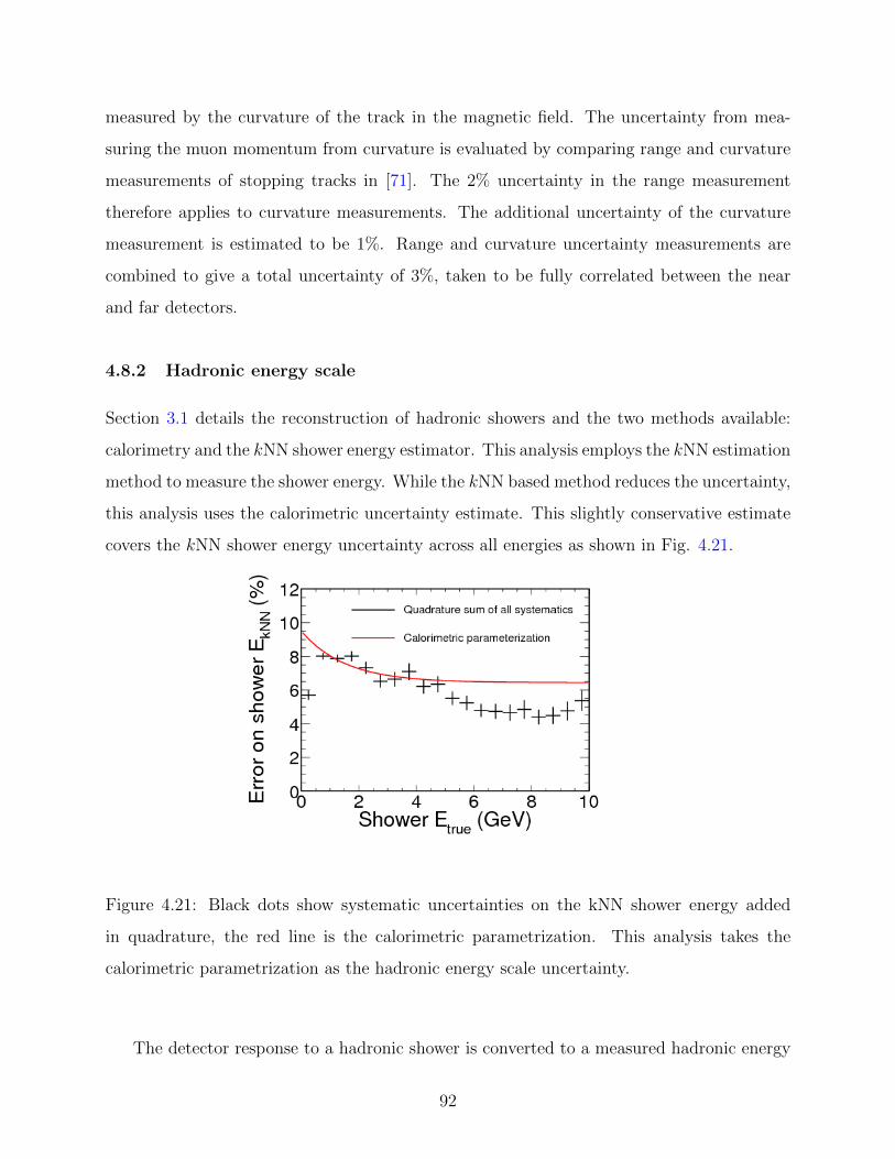
measured by the curvature of the track in the magnetic field. The uncertainty from mea-
suring the muon momentum from curvature is evaluated by comparing range and curvature
measurements of stopping tracks in [71]. The 2% uncertainty in the range measurement
therefore applies to curvature measurements. The additional uncertainty of the curvature
measurement is estimated to be 1%. Range and curvature uncertainty measurements are
combined to give a total uncertainty of 3%, taken to be fully correlated between the near
and far detectors.
4.8.2 Hadronic energy scale
Section 3.1 details the reconstruction of hadronic showers and the two methods available:
calorimetry and the kNN shower energy estimator. This analysis employs the kNN estimation
method to measure the shower energy. While the kNN based method reduces the uncertainty,
this analysis uses the calorimetric uncertainty estimate. This slightly conservative estimate
covers the kNN shower energy uncertainty across all energies as shown in Fig. 4.21.
Figure 4.21: Black dots show systematic uncertainties on the kNN shower energy added
in quadrature, the red line is the calorimetric parametrization. This analysis takes the
calorimetric parametrization as the hadronic energy scale uncertainty.
The detector response to a hadronic shower is converted to a measured hadronic energy
92

by the calibration procedure described in Section 3.2. There are two ways in which this
conversion may be erroneous, and thus two sources of uncertainty on the shower energy
measurement: a relative uncertainty from the difference in the calibration between Near and
Far detectors, and an absolute uncertainty in the conversion factors of detector response to
hadronic energy.
The relative uncertainty is accounted for by evaluating the difference between data and
simulation at various steps of calibration and determined to be 1.85% in the Near Detector
and 1.05% in the Far. The relative uncertainty is fully uncorrelated between the detectors.
The absolute uncertainty has two components. First, there is a 5.7% uncertainty in the
conversion of CalDet response to hadronic shower energy. Second, there are uncertainties
arising from modeling the hadron production. The size of this uncertainty is energy de-
pendent since the models’ performance varies across energy ranges. Adding the 5.7% from
CalDet response to this energy dependent in quadrature, the total uncertainty on the shower
energy can be parametrized as [97],
σhad = 6.6% + 3.5%× exp
(−Ehad
1.44GeV
). (4.7)
4.8.3 Relative normalization
The relative near/far normalization uncertainty consists of several components summarized
in [98]. The three largest contributions to this uncertainty come from near/far selection bias
(1.3%), near detector fiducial bias (0.7%) and far detector livetime (0.32%). The near/far
selection bias uncertainty comes from the difference between Near and Far Detector recon-
struction efficiencies. The double ratio,
R =εFDData/ε
FDMC
εNDData/εNDMC
(4.8)
where ε is the reconstruction efficiency would be equal to 1.0 if there were no modeling
differences. The size of this uncertainty was evaluated by a manual scan of thousands
of events. Scanners looked for missed tracks, miscalculated energies, fake tracks, charge
misidentification and general reconstruction pathologies. The ND fiducial bias uncertainty
93

accounts for differences in agreement between data and Monte Carlo in different regions
of the ND fiducial volume. This is done by dividing the fiducial volume into two along
x, y, and z directions and evaluating the asymmetry in the ratio of data to Monte Carlo
between halves. Far detector livetime uncertainty accounts for the far detector inefficiency
quantified by the difference between POT counts obtained by two methods; 0.32% is the
difference between POTs from data files and POTs from the database. Table 4.1 shows the
components of the Near/Far normalization uncertainty.
Systematic Contribution to relative uncertainty (%)
Steel thickness 0.2
Scintillator thickness 0.2
FD livetime 0.32
ND fiducial bias 0.70
N/F selection bias 1.3
Sum in quadrature 1.54
Table 4.1: Contributions to the relative near/far normalization uncertainty, taken from [98].
4.8.4 Backgrounds
The uncertainty in neutral-current (NC) background modeling arises primarily from hadronic
shower modeling. The systematic uncertainty on NC background was evaluated by compar-
ing data to MC events in the NC-dominated region (the region of kNNID < 0.3). If the
entire disagreement between data and Monte Carlo is attributed to the NC background, a
20% uncertainty covers the discrepancy.
There is an uncertainty associated with true neutrino events that are mis-identified as
antineutrinos due to a charge sign measurement error. This mis-identified component is
dominant for events with a large error in the q/p measurement, which is quantified as
σ(q/p)/(q/p) > 2.3, where σ(q/p) is the uncertainty on the q/p measurement. To evalu-
ate the size of this systematic the entire discrepancy between data and simulation in this
94
subset of events is attributed to mis-identified charge sign. A maximum scale of ±30% is
required to make data and MC agree as a function of energy, so an uncertainty of 30% was
taken on this background component.
4.8.5 Cross section uncertainties
There are four components that go into the cross-section uncertainty: quasi-elastic, reso-
nance, deep-inelastic scattering (DIS) and total cross-section.
• Quasi-elastic and Resonance cross-section uncertainty. MINOS models the cross
sections in this regime by the axial-vector masses MQEA and MRes
A . Taking into account
the uncertainty in the data used to obtain the best information on these parameters and
nuclear effects, a ±15% error is estimated on MResA and ±30% on MQE
A .
• Total cross section. Fits to world CC νµ cross section data in the 10-30 GeV range
yield an estimate of 3.5% for normalization of the overall CC interaction cross section.
• Cross sections in the Resonance/DIS Transition Region. This uncertainty comes
from the uncertainty on the parameters of the neutrino event generator, NEUGEN. The
error is estimated by a combination of fits to experimental data and variations in the fit
with changes in the interaction model parameters.
The uncertainties are evaluated by varying the parameters in the cross section model.
Antineutrino cross sections have larger uncertainties so an additional set of uncertainties is
considered only for antineutrinos. Details of cross-section uncertainties are given in [99].
4.8.6 Smaller sources of systematic uncertainties
Beam modeling The beam modeling uncertainty arises primarily from uncertainties in the
hadron production model as well as beam optics, horn current, horn position, target position,
and the shape and amount of material in the horns. The total error that results has been
evaluated in [100] for each neutrino run period and adapted for antineutrino-mode running.
Beam modeling uncertainties cancel nearly entirely between the two detectors because the
95
beam is measured at the Near Detector and the Far Detector prediction is obtained from
this.
Near Detector Acceptance In order to evaluate the uncertainty on Near Detector accep-
tance which was not included in previous oscillation analyses, a special run was performed
operating the Near Detector coil in reverse polarity so that µ+ tracks from antineutrino inter-
actions are de-focused. The ratio of Far Detector predictions obtained from regular, focused
ND data and this special de-focused data provides an error band that is incorporated as an
uncertainty in this analysis.
4.9 FAR DETECTOR SELECTION
The Far Detector sample is selected by the CC/NC separation and charge sign selection as
the ND. In order to remove contamination from cosmic muons, tracks are required to have
at most an angle θ with the beam axis such that cos θ < 0.6. The overall efficiency of this
selector and contamination before and after selection at the Far Detector is shown in Fig.
4.22.
This is a blind analysis, meaning any far detector data spectrum that holds the possibil-
ity of revealing the magnitude of oscillations is not studied until the entire analysis chain is
finalized. Since oscillations will manifest as a disappearance in the far detector data, these
spectra are handled with extra care. It is still necessary to check that data is well modeled
by the Monte Carlo simulation. To accomplish this we only look at far detector distribu-
tions of variables that are insensitive to oscillations, such as spatial distributions, and the
overall normalization of the event count is hidden. In order to study oscillation-sensitive
distributions, such as energies and kinematic variables, a blinding algorithm is applied to
data which removes a subset of the events from the dataset in a way that will mask the
effect of oscillations. After the analysis is finalized, unblinded and events are counted, the
properly normalized versions of these comparisons are performed with the full dataset.
With 2.95 × 10²⁰ POT of exposure, a total of 273 antineutrino events are expected at
the Far Detector in the case of no oscillations and 193 antineutrino events are observed.
96
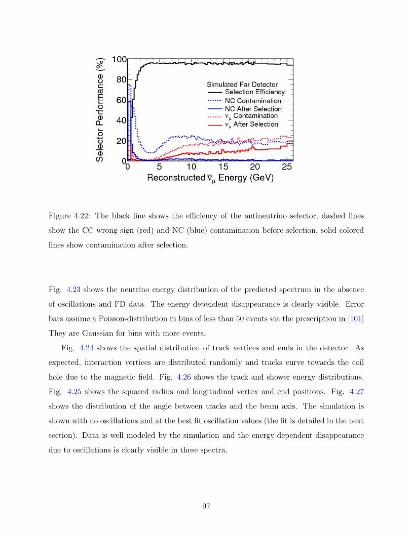
Figure 4.22: The black line shows the efficiency of the antineutrino selector, dashed lines
show the CC wrong sign (red) and NC (blue) contamination before selection, solid colored
lines show contamination after selection.
Fig. 4.23 shows the neutrino energy distribution of the predicted spectrum in the absence
of oscillations and FD data. The energy dependent disappearance is clearly visible. Error
bars assume a Poisson-distribution in bins of less than 50 events via the prescription in [101]
They are Gaussian for bins with more events.
Fig. 4.24 shows the spatial distribution of track vertices and ends in the detector. As
expected, interaction vertices are distributed randomly and tracks curve towards the coil
hole due to the magnetic field. Fig. 4.26 shows the track and shower energy distributions.
Fig. 4.25 shows the squared radius and longitudinal vertex and end positions. Fig. 4.27
shows the distribution of the angle between tracks and the beam axis. The simulation is
shown with no oscillations and at the best fit oscillation values (the fit is detailed in the next
section). Data is well modeled by the simulation and the energy-dependent disappearance
due to oscillations is clearly visible in these spectra.
97
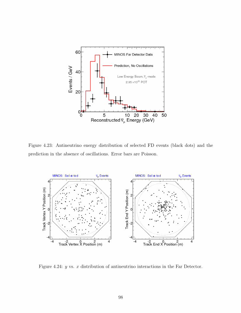
Figure 4.23: Antineutrino energy distribution of selected FD events (black dots) and the
prediction in the absence of oscillations. Error bars are Poisson.
Figure 4.24: y vs. x distribution of antineutrino interactions in the Far Detector.
98

Figure 4.25: Top plots show the squared track vertex (left) and end radii in meters. Bottom
plots show the longitudinal track vertex (left) and end positions in units of number of planes.
Black dots represent FD data, the solid red curve represents Monte Carlo with oscillations
and dashed curve is without oscillations.
99

Figure 4.26: Muon track and shower energy distributions of selected antineutrino events
in the Far Detector. The dashed red line shows the predicted spectrum in the absence of
oscillations, the solid red line is the prediction at the best fit and black dots show data with
Poisson error bars.
Figure 4.27: Distribution of the cosine of the angle between tracks and the beam axis. Events
with cos θ < 0.6 are excluded. Black dots represent FD data, the solid red curve represents
Monte Carlo with oscillations and dashed curve is without oscillations.
100
4.10 FITTING THE DATA
The measured far detector energy spectrum is fit to the two flavor vacuum oscillation model
from Section 1.3, in which the disappearance probability of a muon neutrino is given Eq.
(4.9) by,
Pνµ→νµ = sin2 2(θ23
)sin2
(1.27
∆m232L
E
). (4.9)
The best fit to data is calculated by minimizing the standard log-likelihood function
between data and predictions generated over a grid of ∆m2, sin2 2θ sets as shown in Eq.
(4.10). The fit is performed in 100 bins, i, for each run period r. The value of the mixing
angle is constrained to be physical, that is, the allowed range is 0 < sin2(2θ) < 1.
−2 lnλ = 22∑r=1
100∑i=1
npredri − ndata
ri lnndatari
npredri
(4.10)
Confidence intervals and allowed regions in (∆m2,sin2 2θ) space are computed by us-
ing the Feldman-Cousins (FC) method [102, 103]. The ∆χ2 that corresponds to a certain
Gaussian coverage is known analytically from statistics [18]. The FC method is a frequentist
approach where this coverage is calculated by running a large number of pseudo-experiments
at each point and determining what value of ∆χ2 covers the desired percentage of experi-
ments. There are three concerns that the use of the Feldman-Cousins prescription alleviates
[68]. First, parameters are being measured near physical boundaries at sin2 2θ=0,1 and
∆m2=0, where Gaussian confidence intervals are too conservative (over-coverage). Second,
a high ∆m2 affects the event rate in the same way as sin2 2θ≈ 0.5. There is a difference
in the low energy spectra these two effects produce but with a small dataset this difference
is not resolved. This gives rise to a degeneracy which results in under-coverage if Gaussian
confidence intervals are used. Finally, using the Feldman-Cousins method allows the effect
of systematic uncertainties to be included in the confidence contours.
Each point on the likelihood surface corresponds to a (∆m2, sin2 2θ) pair. To obtain the
∆χ2 which corresponds to a certain coverage at a given point, a large number of pseudo-
experiments are generated assuming that true non-standard oscillation parameters are at
101
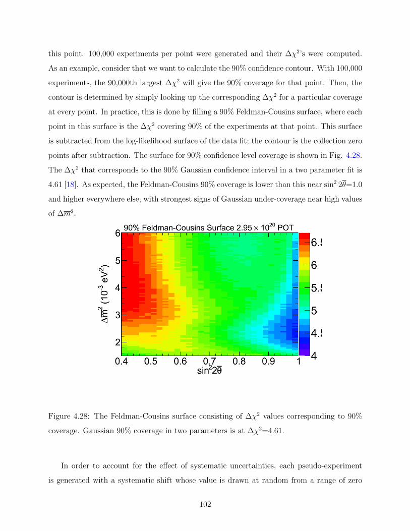
this point. 100,000 experiments per point were generated and their ∆χ2’s were computed.
As an example, consider that we want to calculate the 90% confidence contour. With 100,000
experiments, the 90,000th largest ∆χ2 will give the 90% coverage for that point. Then, the
contour is determined by simply looking up the corresponding ∆χ2 for a particular coverage
at every point. In practice, this is done by filling a 90% Feldman-Cousins surface, where each
point in this surface is the ∆χ2 covering 90% of the experiments at that point. This surface
is subtracted from the log-likelihood surface of the data fit; the contour is the collection zero
points after subtraction. The surface for 90% confidence level coverage is shown in Fig. 4.28.
The ∆χ2 that corresponds to the 90% Gaussian confidence interval in a two parameter fit is
4.61 [18]. As expected, the Feldman-Cousins 90% coverage is lower than this near sin2 2θ=1.0
and higher everywhere else, with strongest signs of Gaussian under-coverage near high values
of ∆m2.
Figure 4.28: The Feldman-Cousins surface consisting of ∆χ2 values corresponding to 90%
coverage. Gaussian 90% coverage in two parameters is at ∆χ2=4.61.
In order to account for the effect of systematic uncertainties, each pseudo-experiment
is generated with a systematic shift whose value is drawn at random from a range of zero
102
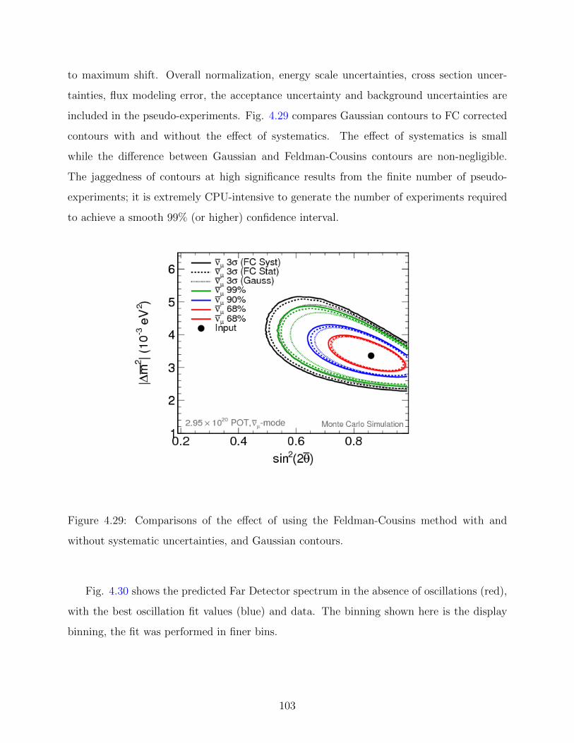
to maximum shift. Overall normalization, energy scale uncertainties, cross section uncer-
tainties, flux modeling error, the acceptance uncertainty and background uncertainties are
included in the pseudo-experiments. Fig. 4.29 compares Gaussian contours to FC corrected
contours with and without the effect of systematics. The effect of systematics is small
while the difference between Gaussian and Feldman-Cousins contours are non-negligible.
The jaggedness of contours at high significance results from the finite number of pseudo-
experiments; it is extremely CPU-intensive to generate the number of experiments required
to achieve a smooth 99% (or higher) confidence interval.
Figure 4.29: Comparisons of the effect of using the Feldman-Cousins method with and
without systematic uncertainties, and Gaussian contours.
Fig. 4.30 shows the predicted Far Detector spectrum in the absence of oscillations (red),
with the best oscillation fit values (blue) and data. The binning shown here is the display
binning, the fit was performed in finer bins.
103

The set of parameter values that best fit the data are
|∆m2atm| = 2.62+0.31
−0.28(stat.)± 0.09(syst.)× 10−3eV2
sin2(2θ)23 = 0.95+0.10−0.11(stat.)± 0.01(syst.) (4.11)
sin2(2θ)23 > 0.75 (90%C.L.) (4.12)
The statistical errors on the above numbers are the 1σ errors from the one-parameter
Gaussian fits to each parameter. Note that the sign of |∆m2atm| cannot be distinguished
because its squared sine appears in the oscillation probability formula. The contours shown
in Fig. 4.31 are obtained by subtracting the corresponding FC surfaces as explained above.
Figure 4.30: Far detector νµdata and predictions with no oscillations (red histogram) and
with the best-fit oscillation parameters (blue histogram). The band around the oscillated
prediction represents the total systematic uncertainty. Total background in the oscillated
prediction is also displayed (gray shaded histogram). The data and predictions correspond
to an exposure of 2.95× 10²⁰ POT.
104

Figure 4.31: The 68%, 90%, and 99% antineutrino oscillation contours. The contours are de-
termined using the Feldman-Cousins method. The best fit is at |∆m2atm| = 2.62+0.31
−0.28(stat.)±
0.09(syst.)× 10−3eV2 and sin2(2θ23) = 0.95+0.10−0.11(stat.)± 0.01(syst.).
4.10.1 Evaluation of Oscillation Parameter Uncertainties
The effect of systematic uncertainties are calculated by generating a set of systematically
shifted fake data for each run period, as well as an unshifted (nominal) set. Generated
events are treated like real data and passed through the entire analysis chain to fit for
oscillation parameters. In fitting these systematically shifted pseudo-datasets, the value of
sin2(2θ) is not constrained to be physical. The difference between the best fit values of a
shifted dataset to the nominal data set is calculated. Systematically shifted fake data were
generated with oscillation parameters |∆m2| = 2.62 × 10⁻³ eV2 and sin2(2θ) = 0.947 [104].
Fig. 4.32 shows the effect of these shifts graphically. The largest systematic uncertainties in
the mass-splitting measurement are muon and hadronic energy scale. For mixing angle the
largest effect comes from Near/Far normalization. Tables 4.2 lists the best fits to nominal
105

and shifted datasets and the differences between the two numerically.
Figure 4.32: The deviations in the best fit parameters from their nominal positions when
the analysis is performed on systematically shifted datasets.
To study the effect of systematic uncertainty on the number of predicted Far Detector νµ
events, systematically shifted high statistics near and far detector fake datasets are created
from Monte Carlo. A far detector prediction is generated from each systematically shifted
near detector fake data set using identical oscillation parameters to the fake data. The
prediction is scaled to 2.95×10²⁰ protons on target. To obtain the total fractional systematic
error in the number of events at the far detector, the double ratio
1− Shifted FD Prediction / Shifted FD Fake Data
Nominal FD Prediction / Nominal FD Fake Data(4.13)
is calculated for each systematic shift. The shifted far detector fake data encapsulates the
effect of systematic uncertainties on the far detector. The shifted far detector prediction is
obtained by extrapolating the shifted near detector fake data and thus reflects the systematics
at the near detector. The above ratio therefore takes into account cancellations between the
106

near and far detectors. In each energy bin, positive values of expression (4.13) are added in
quadrature to obtain the upper and negative values to give the lower systematic error band.
The resulting systematic error band is shown in Fig. 4.33.
Figure 4.33: The total systematic error band on the number of predicted νµ events. The
band is obtained by adding the effect of each individual systematic shift on the FD predicted
energy spectrum in quadrature.
While systematic uncertainties have been treated with care and their effects taken into
account in the fit, this is a highly statistics-limited analysis. Fig. 4.34 compares the size
of systematic shifts to the statistical sensitivity. The statistical size of allowed regions com-
pletely cover the systematics which are miniscule on this scale.
107

Figure 4.34: The effect of systematics shown in Fig. 4.32 overlaid with the statistical sensi-
tivity.
108
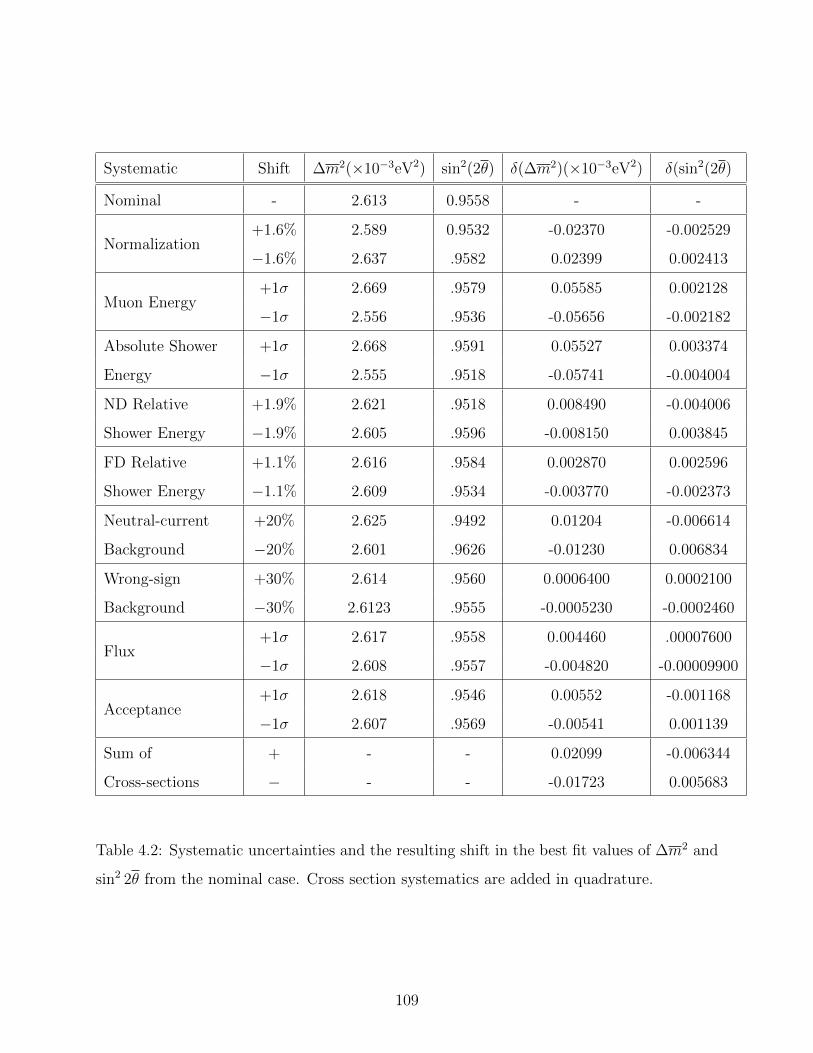
Systematic Shift ∆m2(×10−3eV2) sin2(2θ) δ(∆m2)(×10−3eV2) δ(sin2(2θ)
Nominal - 2.613 0.9558 - -
Normalization+1.6% 2.589 0.9532 -0.02370 -0.002529
−1.6% 2.637 .9582 0.02399 0.002413
Muon Energy+1σ 2.669 .9579 0.05585 0.002128
−1σ 2.556 .9536 -0.05656 -0.002182
Absolute Shower
Energy
+1σ 2.668 .9591 0.05527 0.003374
−1σ 2.555 .9518 -0.05741 -0.004004
ND Relative
Shower Energy
+1.9% 2.621 .9518 0.008490 -0.004006
−1.9% 2.605 .9596 -0.008150 0.003845
FD Relative
Shower Energy
+1.1% 2.616 .9584 0.002870 0.002596
−1.1% 2.609 .9534 -0.003770 -0.002373
Neutral-current
Background
+20% 2.625 .9492 0.01204 -0.006614
−20% 2.601 .9626 -0.01230 0.006834
Wrong-sign
Background
+30% 2.614 .9560 0.0006400 0.0002100
−30% 2.6123 .9555 -0.0005230 -0.0002460
Flux+1σ 2.617 .9558 0.004460 .00007600
−1σ 2.608 .9557 -0.004820 -0.00009900
Acceptance+1σ 2.618 .9546 0.00552 -0.001168
−1σ 2.607 .9569 -0.00541 0.001139
Sum of
Cross-sections
+ - - 0.02099 -0.006344
− - - -0.01723 0.005683
Table 4.2: Systematic uncertainties and the resulting shift in the best fit values of ∆m2 and
sin2 2θ from the nominal case. Cross section systematics are added in quadrature.
109
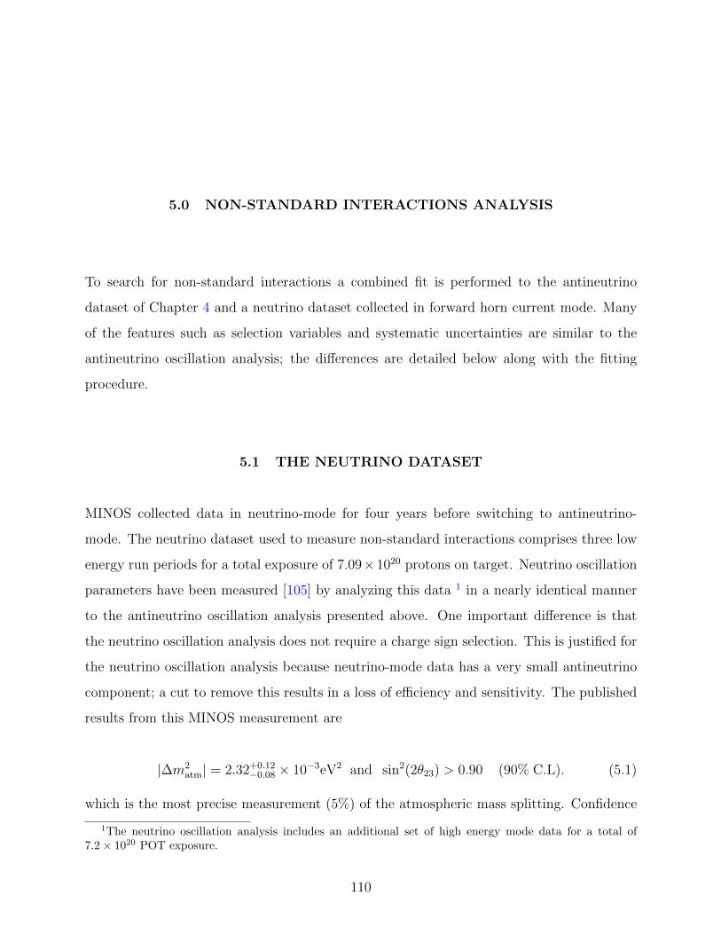
5.0 NON-STANDARD INTERACTIONS ANALYSIS
To search for non-standard interactions a combined fit is performed to the antineutrino
dataset of Chapter 4 and a neutrino dataset collected in forward horn current mode. Many
of the features such as selection variables and systematic uncertainties are similar to the
antineutrino oscillation analysis; the differences are detailed below along with the fitting
procedure.
5.1 THE NEUTRINO DATASET
MINOS collected data in neutrino-mode for four years before switching to antineutrino-
mode. The neutrino dataset used to measure non-standard interactions comprises three low
energy run periods for a total exposure of 7.09×10²⁰ protons on target. Neutrino oscillation
parameters have been measured [105] by analyzing this data 1 in a nearly identical manner
to the antineutrino oscillation analysis presented above. One important difference is that
the neutrino oscillation analysis does not require a charge sign selection. This is justified for
the neutrino oscillation analysis because neutrino-mode data has a very small antineutrino
component; a cut to remove this results in a loss of efficiency and sensitivity. The published
results from this MINOS measurement are
|∆m2atm| = 2.32+0.12
−0.08 × 10⁻³eV2 and sin2(2θ23) > 0.90 (90% C.L). (5.1)
which is the most precise measurement (5%) of the atmospheric mass splitting. Confidence
1The neutrino oscillation analysis includes an additional set of high energy mode data for a total of7.2× 1020 POT exposure.
110

intervals are shown in Fig. 5.1 overlaid with results from the Super Kamiokande experiment.
Detailed accounts of the steps of the neutrino oscillation analysis are presented in [79, 106,
107, 108, 109].
Figure 5.1: Charged-current neutrino oscillation contours are shown in black. Blue and red
curves show contours from Super-K [54].
5.1.1 Separation of charged-current and neutral-current events
In addition to the kNN separator used in the antineutrino oscillation analysis, the neutrino
selection employs a second CC/NC separation method to increase efficiency in the low energy
region. This second separator also uses a kNN algorithm tailored uniquely to the needs of
short tracks, with the purpose of increasing the acceptance of short charged current tracks
without introducing a large neutral current background. The kNN space is constructed by
three variables.
111
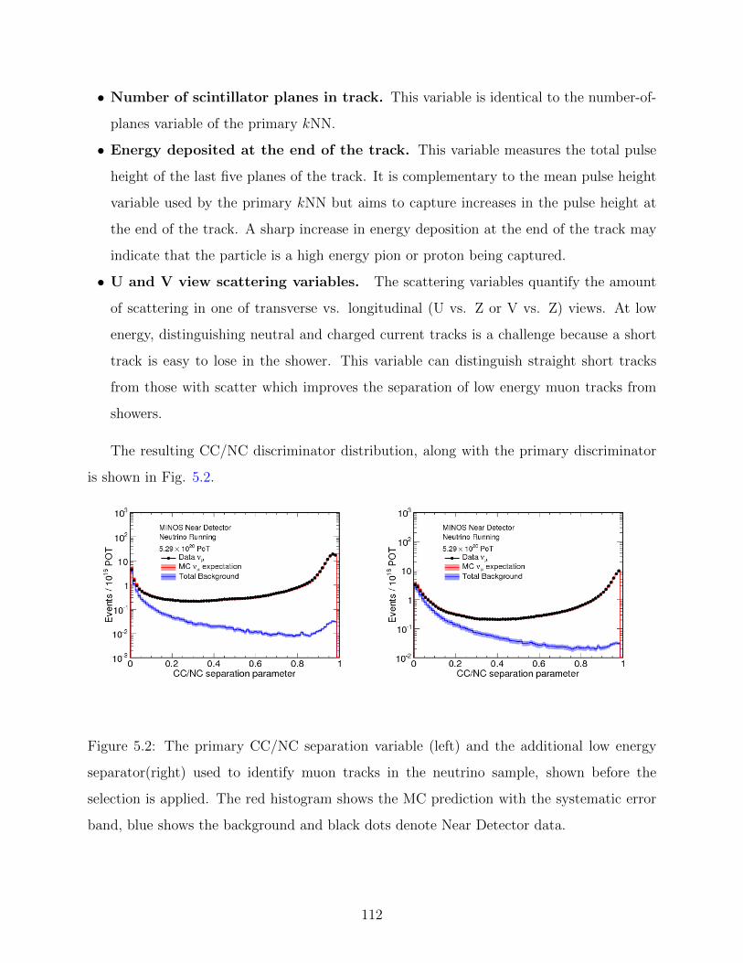
• Number of scintillator planes in track. This variable is identical to the number-of-
planes variable of the primary kNN.
• Energy deposited at the end of the track. This variable measures the total pulse
height of the last five planes of the track. It is complementary to the mean pulse height
variable used by the primary kNN but aims to capture increases in the pulse height at
the end of the track. A sharp increase in energy deposition at the end of the track may
indicate that the particle is a high energy pion or proton being captured.
• U and V view scattering variables. The scattering variables quantify the amount
of scattering in one of transverse vs. longitudinal (U vs. Z or V vs. Z) views. At low
energy, distinguishing neutral and charged current tracks is a challenge because a short
track is easy to lose in the shower. This variable can distinguish straight short tracks
from those with scatter which improves the separation of low energy muon tracks from
showers.
The resulting CC/NC discriminator distribution, along with the primary discriminator
is shown in Fig. 5.2.
Figure 5.2: The primary CC/NC separation variable (left) and the additional low energy
separator(right) used to identify muon tracks in the neutrino sample, shown before the
selection is applied. The red histogram shows the MC prediction with the systematic error
band, blue shows the background and black dots denote Near Detector data.
112

5.1.2 Near Detector Sample
The charged-current selection is a logical OR of the two kNN discriminators where events
with kNNID > 0.25 or kNNnewID > 0.5 are kept. CC neutrino interactions have a µ− in the
final state therefore the charge sign requirement is q/p < 0. The track end point requirement
to cut out the coil hole region is not held for this analysis. The efficiency and contamination
of the overall neutrino selection is shown in Fig. 5.3 at the Near Detector.
Figure 5.3: The black line shows the efficiency of the neutrino selector, dashed lines show
the antineutrino (red) and NC (blue) contamination before selection, solid colored lines show
contamination after selection.
Fig. 5.4 shows the neutrino energy, track energy, shower energy and inelasticity distri-
butions. The red band shows the Monte Carlo with a systematic error band calculated by
adding the effect of each systematic uncertainty in quadrature; details of systematic uncer-
tainties are given in Section 4.8 and 5.4. The band includes the effects of the uncertainty
in the beam flux and neutrino cross sections, which mostly cancel between the two detec-
tors and have a negligible impact on the results. The blue band shows the size of the total
background consisting of mis-identified tracks of opposite sign and neutral-current events.
The data shows good agreement with Monte Carlo and the disagreements are within limits
of the systematic error.
113

Figure 5.4: Neutrino energy (top left), track energy (top right), shower energy (bottom
left) and inelasticity distributions at the Near Detector for the neutrino sample. Black dots
represent ND data, red curve represents Monte Carlo where the pink band is the systematic
error. The blue band shows the total background of neutral current and wrong-sign events.
114

Fig. 5.5 shows the squared radius and longitudinal distributions of track vertices. Many
other distributions including distributions of track shapes and sizes, kinematic variables,
angular distributions and timing were investigated; Monte Carlo models data well.
Figure 5.5: The squared track vertex (left) position in meters and the longitudinal track
vertex position in units of number of planes. Black dots represent ND data and the red
curve represents Monte Carlo.
115

5.1.3 Far Detector Sample
The Far Detector selection is the same as the Near with the additional requirement that
the cosine of the angle between the track direction and beam axis is smaller than 0.6. The
efficiency and contamination of the overall neutrino selection is shown in Fig. 5.6 at the Far
Detector.
Figure 5.6: The black line shows the efficiency of the neutrino selector, dashed lines show the
antineutrino (red) and neutral current (blue) contamination before selection, solid colored
lines show contamination after selection at the Far Detector.
With 7.09× 10²⁰ POT of neutrino data, a total of 2073 events are expected in the case
of no oscillations; we observe 1654 events. Track vertex and end distributions are shown in
Fig. 5.7. Track vertices have a flat squared radius distribution as expected. Tracks curve
towards the coil hole. The track and shower energy distributions can be seen in Fig. 5.8 and
present good agreement between data and simulation. The distribution of the angle that
tracks make with the beam axis is shown in Fig. 5.9. Error bars are Poisson for bins with
fewer than 50 events as prescribed by [101].
116

Figure 5.7: Track vertex and end squared radius distributions of the neutrino sample at the
Far Detector. The dashed red curve is the Monte Carlo simulation with no oscillations, the
solid red curve is best vacuum oscillation fit and black dots are data.
117
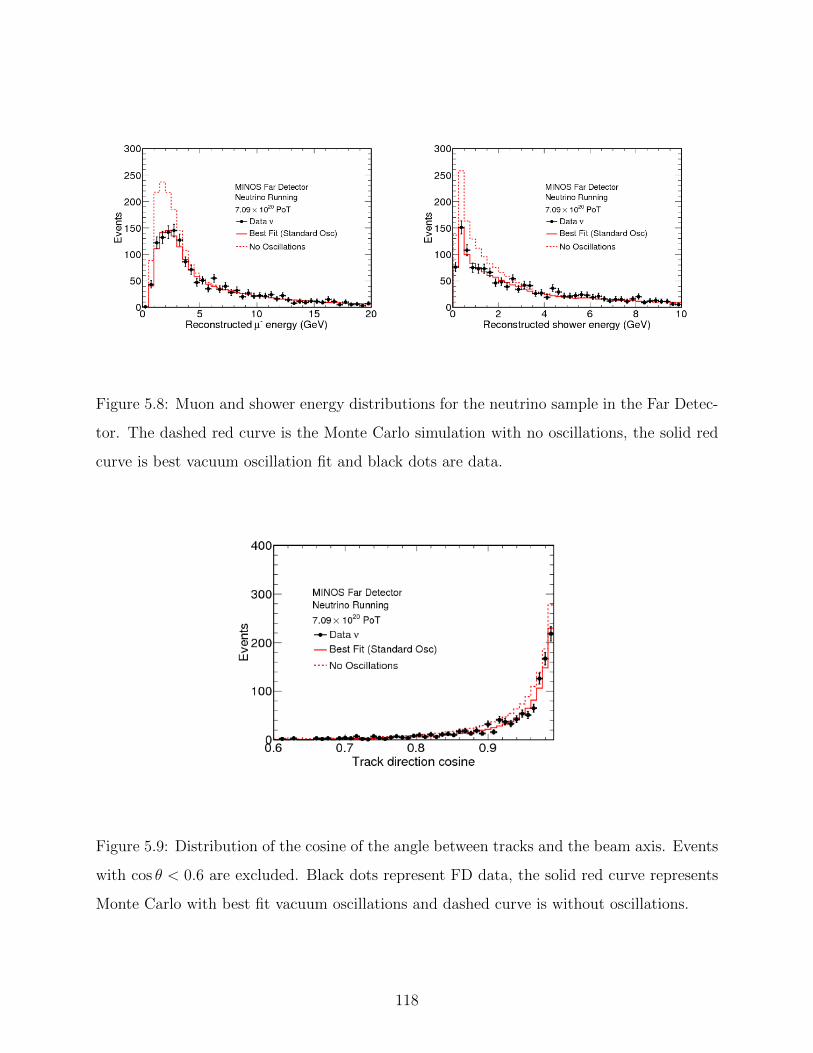
Figure 5.8: Muon and shower energy distributions for the neutrino sample in the Far Detec-
tor. The dashed red curve is the Monte Carlo simulation with no oscillations, the solid red
curve is best vacuum oscillation fit and black dots are data.
Figure 5.9: Distribution of the cosine of the angle between tracks and the beam axis. Events
with cos θ < 0.6 are excluded. Black dots represent FD data, the solid red curve represents
Monte Carlo with best fit vacuum oscillations and dashed curve is without oscillations.
118
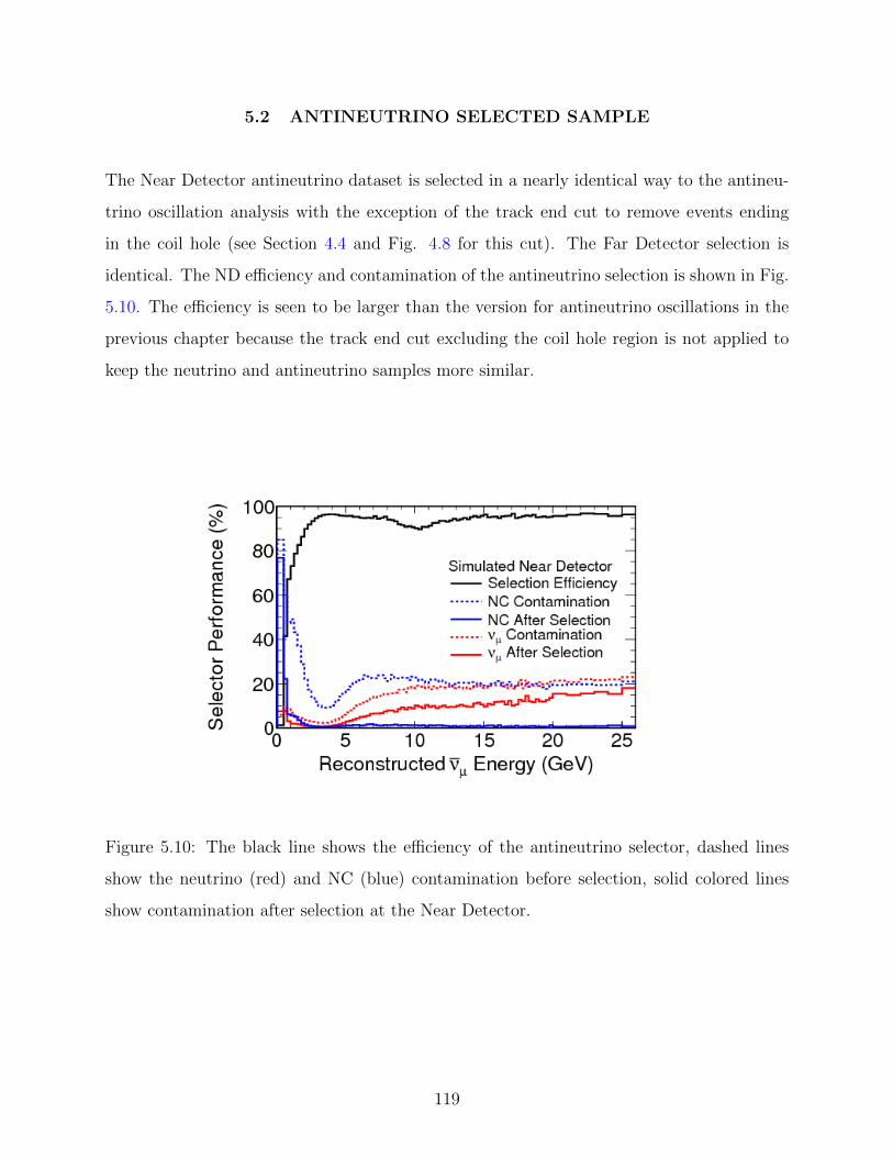
5.2 ANTINEUTRINO SELECTED SAMPLE
The Near Detector antineutrino dataset is selected in a nearly identical way to the antineu-
trino oscillation analysis with the exception of the track end cut to remove events ending
in the coil hole (see Section 4.4 and Fig. 4.8 for this cut). The Far Detector selection is
identical. The ND efficiency and contamination of the antineutrino selection is shown in Fig.
5.10. The efficiency is seen to be larger than the version for antineutrino oscillations in the
previous chapter because the track end cut excluding the coil hole region is not applied to
keep the neutrino and antineutrino samples more similar.
Figure 5.10: The black line shows the efficiency of the antineutrino selector, dashed lines
show the neutrino (red) and NC (blue) contamination before selection, solid colored lines
show contamination after selection at the Near Detector.
119

5.3 NEAR TO FAR EXTRAPOLATION
The extrapolation procedure is explained in detail in Section 4.7. This analysis uses the
same extrapolation method. The measured Near Detector data is extrapolated by using the
Beam Matrix method to obtain a Far Detector prediction. Neutrinos and antineutrinos are
extrapolated separately to take into account the differences in the background, but neutrino
and antineutrino mass-splittings and mixing angles are always taken to be identical. Within
the neutrino sample, each run is extrapolated separately to account for flux differences due
to target decay and for the presence of Helium in the decay pipe in Run III.
5.4 SYSTEMATIC UNCERTAINTIES
The set of uncertainties that can affect disappearance measurements are given in Section 4.8
in detail. The same set of uncertainties applies to this measurement, with two exceptions.
The acceptance systematic is not taken into consideration in this analysis. Also, the wrong
sign background uncertainty has different magnitudes for the neutrino and antineutrino
samples.
The wrong-sign background uncertainty of the antineutrino sample is described in Section
4.8.4. The antineutrino background uncertainty in the neutrino sample is evaluated similarly
to be 70%. The antineutrino component in neutrino-mode is much smaller, so although there
is a larger percentage uncertainty, its effect on the result is still small (indeed smaller than
the wrong-sign uncertainty in the antineutrino sample).
The neutral current background uncertainty in the neutrino sample is 20% (see Sec-
tion 4.8.4). In the neutrino sample, a data-driven method is used to evaluate the size of
this uncertainty [110] and finds the total uncertainty to be 19%, therefore an overall 20%
uncertainty is taken in both neutrino and antineutrino datasets.
120

5.5 FITTING THE DATA
The neutrino and antineutrino data is fit simultaneously to the non-standard interactions
model where the disappearance probability is given by Eq. (1.85). The best fit to data
is calculated by minimizing the log-likelihood function [18] between data and predictions
generated at a range of ∆m2, sin2(2θ), ε sets. The fit is performed in 100 bins, i, and five
run periods, r. The value of the mixing angle is constrained to be physical, that is, the
allowed range is 0 < sin2(2θ) < 1.
Systematic uncertainties are taken into consideration in the fit. As shown in section 5.4,
the overall effect of systematics is much smaller than the statistical uncertainty. However,
the relative statistical size of the neutrino and antineutrino samples is very different (about
1600 neutrino events and 200 antineutrino). The inclusion of the effect of systematics on the
analysis ensures that the neutrino sample does not “pull” the fit disproportionately. System-
atic uncertainties are included in the fit as penalty terms, meaning the fitter is allowed to
vary each systematic uncertainty term (within user-defined limits) to minimize the likelihood
at every grid point. The final likelihood function with systematics is given by
−2 lnλ = 25∑r=1
N∑i=1
npredri − ndata
ri lnndatari
npredri
+4∑
α=1
(Sα − S
′α
σα
)2
(5.2)
where Sα denotes a systematically shifted prediction with systematic α, and σα are the sizes
of the one-sigma level for each uncertainty.
The four largest systematic uncertainties were included in the fit: muon energy scale,
hadronic energy scale, neutral current background and Near to Far normalization. The
systematic error bands in Fig. 5.11 show the fractional effect of the four largest uncertainties
on the Far Detector prediction in the neutrino and antineutrino samples.
From three free parameters, it is possible to construct three two-dimensional likelihood
surfaces. This is performed by marginalizing over the parameter that is not being shown.
To calculate a likelihood surface y vs. x with marginalized parameter z, the likelihood at a
point (xo, yo) is computed by fixing the values of x = xo and y = yo and finding the minimum
of Eq. 5.2 by varying z. The information of the zo that gives the minimum likelihood is lost
121
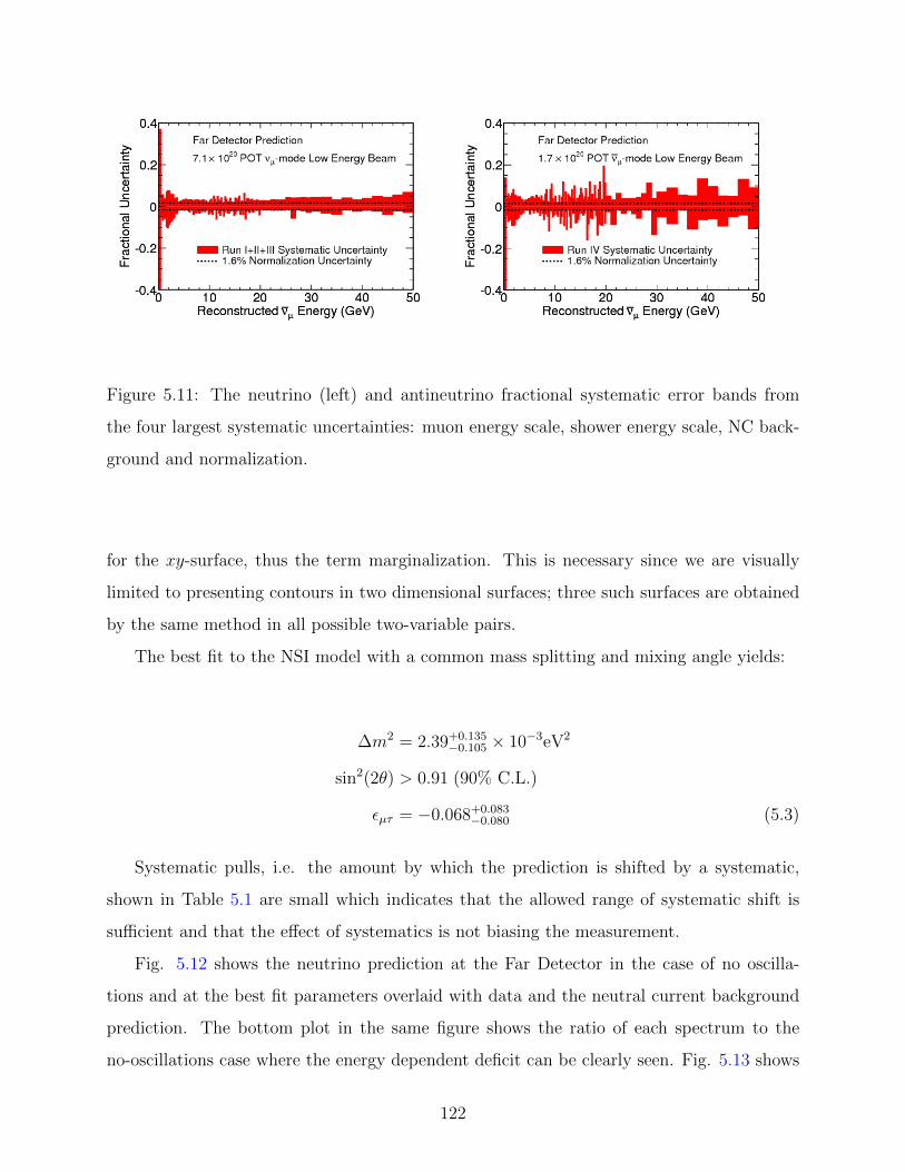
Figure 5.11: The neutrino (left) and antineutrino fractional systematic error bands from
the four largest systematic uncertainties: muon energy scale, shower energy scale, NC back-
ground and normalization.
for the xy-surface, thus the term marginalization. This is necessary since we are visually
limited to presenting contours in two dimensional surfaces; three such surfaces are obtained
by the same method in all possible two-variable pairs.
The best fit to the NSI model with a common mass splitting and mixing angle yields:
∆m2 = 2.39+0.135−0.105 × 10⁻³eV2
sin2(2θ) > 0.91 (90% C.L.)
εµτ = −0.068+0.083−0.080 (5.3)
Systematic pulls, i.e. the amount by which the prediction is shifted by a systematic,
shown in Table 5.1 are small which indicates that the allowed range of systematic shift is
sufficient and that the effect of systematics is not biasing the measurement.
Fig. 5.12 shows the neutrino prediction at the Far Detector in the case of no oscilla-
tions and at the best fit parameters overlaid with data and the neutral current background
prediction. The bottom plot in the same figure shows the ratio of each spectrum to the
no-oscillations case where the energy dependent deficit can be clearly seen. Fig. 5.13 shows
122

the same histograms for the antineutrino sample.
Systematic uncertainty Pull(σ)
Normalization 0.012
Track energy scale −0.017
Shower energy scale −0.17
NC background −0.0091
Table 5.1: Four systematic uncertainties included in the fit and the amount by which the
prediction needs to be shifted by each (“pulls”) to obtain the best fit.
123

Figure 5.12: Top: Far Detector neutrino prediction in the case of no oscillations in red and
at the NSI best fit parameters in blue. Black dots represent data with Poisson error bars.
The gray solid histogram shows the neutral current background. Bottom: The ratio of data
and best fit to null oscillations.
124
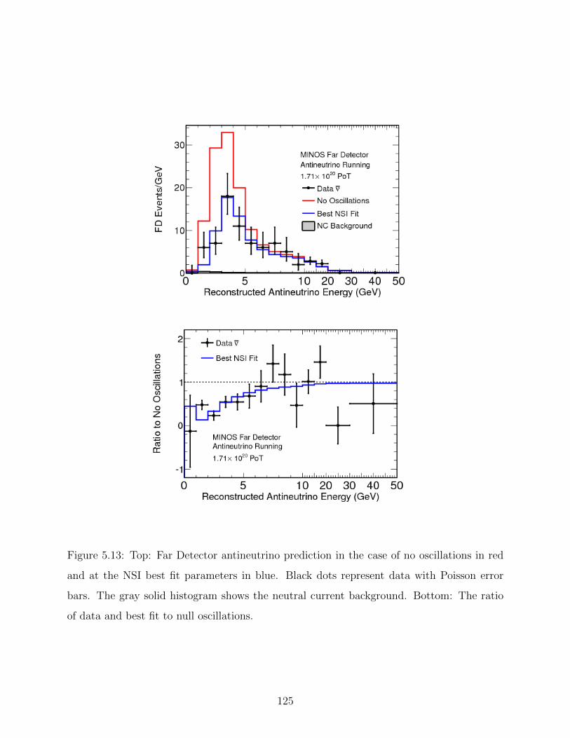
Figure 5.13: Top: Far Detector antineutrino prediction in the case of no oscillations in red
and at the NSI best fit parameters in blue. Black dots represent data with Poisson error
bars. The gray solid histogram shows the neutral current background. Bottom: The ratio
of data and best fit to null oscillations.
125

The χ2per degree of freedom of the fit (in 500 bins with 7 free parameters) is 518/492.
The allowed regions are shown in Fig. 5.14 while Fig. 5.15 shows the one-dimensional allowed
region for each parameter. In these plots, the unshown two variables are marginalized as
described above. The 1 σ errors on the best fit values quoted above come from these ∆χ2
distributions.
Figure 5.14: The 68% and 90% contours include the four largest systematics.
126

Figure 5.15: ∆χ2 for one dimensional fits where all other parameters are marginalized.
Dashed lines show 1, 2 and 3σ coverage.127
5.5.1 Evaluation of NSI parameter Uncertainties
The effect of systematic uncertainties are calculated by generating five sets of systematically
shifted fake data corresponding to the three neutrino and two antineutrino run periods with
each systematic uncertainty, as well as an unshifted set (nominal). Runs I, II and III are
neutrino-mode runs and are produced with the same size systematic, always correlated with
each other. This makes up the shifted neutrino dataset. Shifted Run IV and Run VII
fake data comprise the antineutrino dataset. Combined fits to the shifted neutrino and
antineutrino sets are performed and the shifted best fits are compared to the nominal best
fit point. The difference between nominal and shifted best fit values of each parameter gives
the effect of a given systematic on that parameter. The total systematic uncertainty is
computed by adding the differences in quadrature.
Correlation of each systematic uncertainty between the neutrino and antineutrino sam-
ples is taken into consideration. The wrong sign background systematic is by definition fully
correlated between the two samples. In order to account for partial correlations of other
systematics, the effect of the uncertainty has been evaluated twice, once assuming full corre-
lation and once full uncorrelation. The resulting deviations from the nominal best fit point
in the correlated and uncorrelated evaluations are small and do not affect the overall size of
the systematic uncertainty significantly. Moreover, the analysis is limited by statistics and
the neutrino-antineutrino correlations of systematics have no effect on the extrapolation or
fit results. With this verification, uncertainties are assumed to be fully correlated between
neutrino and antineutrino samples since this makes the computationally simplest fitter.
Table 5.2 shows the nominal and shifted best fit points and the sizes of deviations from
nominal with each systematic. These deviations can be seen graphically in Fig. 5.16. In-
dividual fits to these shifted sets of data are performed to evaluate the relative size of the
effect of each systematic and to graphically compare to the size of the statistical uncertainty.
The incorporation in the fitting mechanism is separate as described above in Sec. 5.5.
128

Systematic Shift ∆m2 sin2 θ εµτ δ(∆m2) δ(sin2 θ) δ(εµτ )
Nominal - 2.6482 1.0045 0.2674 0.0000 0.0000 0.0000
Normalization+1.6% 2.6305 1.0025 0.2769 -0.0176 -0.0020 0.0095
−1.6% 2.6657 1.0064 0.2574 0.0175 0.0019 -0.0100
NC Background+20% 2.6582 0.9975 0.2687 0.0101 -0.0070 0.0013
−20% 2.6379 1.0117 0.2662 -0.0103 0.0072 -0.0013
Muon Energy+1σ 2.6903 1.0062 0.2687 0.0422 0.0017 0.0012
−1σ 2.6060 1.0025 0.2663 -0.0422 -0.0020 -0.0011
SKZP+1σ 2.6537 1.0044 0.2653 0.0056 -0.0001 -0.0022
−1σ 2.6420 1.0047 0.2698 -0.0061 0.0002 0.0024
Abs ShwEn+1σ 2.6950 1.0092 0.2598 0.0469 0.0047 -0.0077
−1σ 2.6008 0.9986 0.2762 -0.0473 -0.0060 0.0087
Rel ShwEn N+1.9% 2.6499 1.0012 0.2702 0.0018 -0.0033 0.0027
−1.9% 2.6463 1.0078 0.2648 -0.0019 0.0033 -0.0027
Rel ShwEn F+1.1% 2.6426 1.0020 0.2703 -0.0055 -0.0025 0.0028
−1.1% 2.6535 1.0071 0.2648 0.0053 0.0025 -0.0027
WS Bckg+70/30% 2.6488 1.0044 0.2679 0.0007 -0.0001 0.0005
−70/30% 2.6475 1.0047 0.2670 -0.0007 0.0001 -0.0005
Total Cross Section+ - - - 0.0118 0.0045 0.0039
− - - - -0.0118 -0.0045 -0.0041
Total Uncertainty+ - - - 0.0677 0.0108 0.0143
− - - - -0.0682 -0.0114 -0.0141
Table 5.2: Systematic uncertainties and the resulting shift in the best fit values of ∆m2,
ε and sin2(2θ) from the nominal case assuming all systematics are fully correlated between
neutrino and antineutrino samples. Cross section systematics are added in quadrature.
129
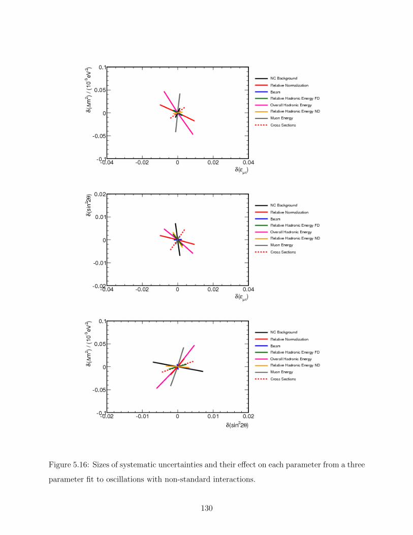
Figure 5.16: Sizes of systematic uncertainties and their effect on each parameter from a three
parameter fit to oscillations with non-standard interactions.
130
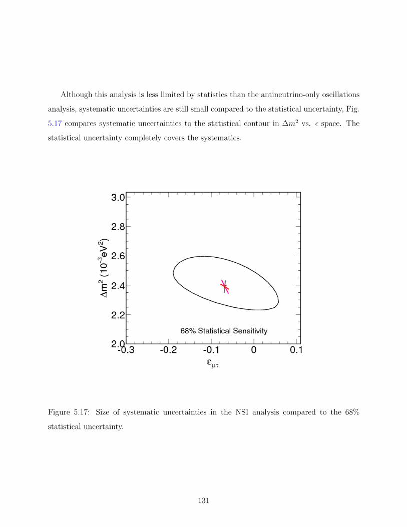
Although this analysis is less limited by statistics than the antineutrino-only oscillations
analysis, systematic uncertainties are still small compared to the statistical uncertainty, Fig.
5.17 compares systematic uncertainties to the statistical contour in ∆m2 vs. ε space. The
statistical uncertainty completely covers the systematics.
Figure 5.17: Size of systematic uncertainties in the NSI analysis compared to the 68%
statistical uncertainty.
131

6.0 CONCLUSION AND OUTLOOK
This thesis presents the most precise long-baseline measurement of muon antineutrino dis-
appearance to date with a tagged νµ beam. The antineutrino dataset collected in two run
periods for a total exposure of 2.95× 10²⁰ POT has been analyzed and found to support the
hypothesis of oscillations. With a no-oscillations expectation of 273 events and an observation
of 193, antineutrino oscillation parameters are measured to be |∆m2atm| = 2.62+0.31
−0.28×10⁻³eV2
and sin2(2θ23) = 0.95+0.10−0.11 with sin2(2θ23) > 0.75 at 90% C.L. This is the most precise mea-
surement to date of the atmospheric mass splitting ∆m2atm. The null oscillation hypothesis
is ruled out at a significance of 7.3σ. Fig. 6.1 shows contours of allowed regions from the
current and previous analyses as well as those of neutrino oscillations.
CPT symmetry requires that masses of particles and their antiparticles be identical. The
mass splitting is therefore expected to be identical for neutrinos in a CPT-conserving scenario
without any non-standard effects. A previous MINOS analysis using only 1.71× 10²⁰ POT
of antineutrino data found parameters of |∆m2atm| = 3.36+0.46
−0.40 × 10⁻³eV2 and sin2(2θ23) =
0.86+0.11−0.12, with which the likelihood that neutrinos and antineutrinos have identical underly-
ing oscillation parameters is 2%. The results of this analysis are in much better agreement
with neutrino oscillations with a 42% statistical likelihood of identical oscillation parame-
ters. The two antineutrino analysis techniques are very similar; it can be concluded that the
previous measurement of a high ∆m2atm is most likely a statistical fluctuation. Contours from
the two separate antineutrino run periods shown in Fig. 6.2 have substantial overlap and lie
on either side of the neutrino oscillation allowed region, converging on a value in agreement
with neutrinos when combined to increase the dataset. This also suggests that the deviation
from the CPT-conserving expectation with small datasets is a statistical effect.
This thesis also uses the 7.1×10²⁰ POT neutrino dataset in combination with the antineu-
132

Figure 6.1: 90% C.L. contours for the previous antineutrino oscillation result published by
MINOS [111] in red and the current measurement in blue, overlaid with the 90% neutrino
contour [105].
trino data to constrain non-standard interactions which would alter the survival probability
as described by Eq. (1.85). No evidence for such non-standard interactions is found. The
best fit to this model gives εµτ = −0.068+0.083−0.080 with a common mass splitting and mixing an-
gle of |∆m2atm| = 2.39+0.135
−0.105 × 10⁻³eV2 and sin223(2θ) > 0.91 (90% C.L.). This measurement
also supports the conclusion that neutrino and antineutrino oscillation parameters agree
within the statistical uncertainty. This result is also in agreement with other measurements
of non-standard interactions [65] as well as values of ε extracted from global fits to data from
multiple experiments [38, 37, 112, 33, 63].
The significance of the non-standard interactions measurement presented here is twofold.
First, it is a direct measurement from a single experiment where the effect of systematics
is well understood and taken into account. Second, neutrino and antineutrino charged-
current interactions can be identified event-by-event in MINOS giving this analysis a unique
133

Figure 6.2: The evolution of the 90% contours of antineutrino oscillation parameters with
increasing data. Shown in black is the latest published result [111] while the gray line shows
the results from the second run only. The blue contour shows the final result presented here.
opportunity to search for an effect that manifests itself as a difference between neutrinos and
antineutrinos.
6.1 FUTURE MEASUREMENTS AND EXPERIMENTS
An upgraded version of MINOS, called MINOS+, will collect data starting in 2013 from
an upgraded NuMI beam which will deliver a higher intensity of higher energy neutrinos
(and antineutrinos) to the NOνA experiment. With the addition of data that spans a wider
range of energies, the experiment has more sensitivity to flavor conserving effects which
manifest as a change in the shape of the energy spectrum rather than a change of the rate
of disappearance. New results on non-standard interactions are expected with this dataset.
134
Neutrino physics in general is ripe for discovery at the time of this writing. Since its
postulation early in this century, studying this elusive particle has improved our understand-
ing of many of its properties while many remain unknown. We do not know the order of
the masses of neutrinos (mass hierarchy), whether or not neutrinos violate CP-symmetry,
or whether they are Dirac or Majorana particles. There are limits of neutrino mass from
neutrino experiments and cosmology but no precise measurements. Developing a thorough
comprehension of neutrino mixing and mass is essential to building a unified theory of particle
physics that bridges the quark and lepton sectors.
The task of answering the many open questions of neutrinos requires multiple ventures:
solar, reactor and accelerator neutrino oscillation experiments, direct mass measurements
and neutrinoless double beta decay. One of the most fundamental of these open questions is
the magnitude of the mixing angle θ13. NOνA [61], T2K [60], Daya Bay [58], Double Chooz
[57] and RENO [59] are some of the experiments that will shed light on this in the next few
years. Knowledge of θ13 allows for an experiment like NOνA to measure the CP-violating
phase δCP and determine the mass hierarchy. Neutrinoless double beta decay experiments
are ongoing; the observation of such a decay would indicate that the neutrino is a Majorana
particle (i.e. its own antiparticle). These and other future experiments will keep advancing
our understanding of neutrinos, improve the Standard Model and further knowledge of the
universe.
135
BIBLIOGRAPHY
[1] O. Hahn and L. Meitner, “Uber die absorption der β-strahlen einiger radioelemente,”Physikalische Zeitschrift, vol. 9, pp. 312–333, 1908.
[2] O. Hahn and L. Meitner, “Uber die β-strahlen des aktiniums,” PhysikalischeZeitschrift, vol. 9, pp. 987–704, 1908.
[3] O. Hahn, L. Meitner, and O. von Baeyer, “Uber die β-strahlen des aktivien nieder-schlags des thoriums,” Physikalische Zeitschrift, vol. 12, pp. 273–279, 1911.
[4] O. Hahn, L. Meitner, and O. von Baeyer, “Nachweis von β-strahlen be radium d,”Physikalische Zeitschrift, vol. 12, pp. 378–379, 1911.
[5] J. Chadwick, “Intensitatsverteilung im magnetischen spektrum der β-strahlen vonradium b + c,” Verhandlungen der deutschen physikalischen Gesellschaft, vol. 16,pp. 383–391, 1914.
[6] C. D. Ellis and W. A. Wooster, “The average energy of disintegration of radium e,” inProceedings of the Royal Society (London), vol. A117, pp. 109–123, 1927.
[7] F. Rasetti, “On the raman effect in diatomic gases,” Proceedings of the NationalAcademy of Sciences of the United States of America, vol. 15, pp. 234–237, March1929.
[8] F. Rasetti, “On the raman effect in diatomic gases. ii,” Proceedings of the NationalAcademy of Sciences of the United States of America, vol. 15, pp. 515–519, June 1929.
[9] W. Pauli. Letter by Wolfgang Pauli to the attendees of the Tubingen conference. Fromthe CERN archive, http://cdsweb.cern.ch/record/83282.
[10] J. Chadwick, “POSSIBLE EXISTENCE OF A NEUTRON,” Nature, vol. 129, p. 312,1932.
[11] F. L. Wilson, “Fermi’s theory of beta decay,” Am. J. Phys, vol. 36, no. 12, 1968.
[12] F. Reines and C. Cowan, “Detection of the free neutrino,” Phys.Rev., vol. 92, pp. 830–831, 1953.
136

[13] C. Cowan, F. Reines, F. Harrison, H. Kruse, and A. McGuire, “Detection of the freeneutrino: A Confirmation,” Science, vol. 124, pp. 103–104, 1956.
[14] M. Goldhaber, L. Grodzins, and A. Sunyar, “HELICITY OF NEUTRINOS,”Phys.Rev., vol. 109, pp. 1015–1017, 1958.
[15] G. Danby et al., “Observation of High-Energy Neutrino Reactions and the Existenceof Two Kinds of Neutrinos,” Phys. Rev. Lett., vol. 9, pp. 36–44, 1962.
[16] T. Patzak, “First direct observation of the tau-neutrino,” Europhys.News, vol. 32,pp. 56–57, 2001.
[17] “Precision electroweak measurements on the Z resonance,” Phys.Rept., vol. 427,pp. 257–454, 2006.
[18] K. Nakamura, “Review of particle physics,” J. Phys., vol. G37, p. 075021, 2010.
[19] M. E. Peskin and D. V. Schroeder, An Introduction To Quantum Field Theory (Fron-tiers in Physics). Westview Press, 1995.
[20] F. Halzen and A. D. Martin, Quarks and Leptons: An Introductory Course in ModernParticle Physics. Wiley, 1984.
[21] B. Pontecorvo, “Inverse beta processes and nonconservation of lepton charge,”Sov.Phys.JETP, vol. 7, pp. 172–173, 1958.
[22] Z. Maki, M. Nakagawa, and S. Sakata, “Remarks on the unified model of elementaryparticles,” Prog.Theor.Phys., vol. 28, pp. 870–880, 1962.
[23] R. Brown, U. Camerini, P. Fowler, H. Muirhead, C. Powell, et al., “Observations withelectron sensitive plates exposed to cosmic radiation. 2,” 1987.
[24] J. Evans, Measuring Antineutrino Oscillations with the MINOS Experiment. PhDthesis, University of Oxford, 2008.
[25] V. Kostelecky and M. Mewes, “Lorentz and CPT violation in the neutrino sector,”Phys.Rev., vol. D70, p. 031902, 2004.
[26] G. Barenboim, L. Borissov, J. D. Lykken, and A. Smirnov, “Neutrinos as the messen-gers of CPT violation,” JHEP, vol. 0210, p. 001, 2002.
[27] G. Barenboim, J. F. Beacom, L. Borissov, and B. Kayser, “CPT violation and thenature of neutrinos,” Phys.Lett., vol. B537, pp. 227–232, 2002.
[28] L. Wolfenstein, “Neutrino oscillations in matter,” Phys. Rev. D, vol. 17, pp. 2369–2374,May 1978.
[29] S. Mikheev and A. Smirnov, “Resonance Amplification of Oscillations in Matter andSpectroscopy of Solar Neutrinos,” Sov.J.Nucl.Phys., vol. 42, pp. 913–917, 1985.
137

[30] G. Gelmini and E. Roulet, “Neutrino masses,” Rept. Prog. Phys., vol. 58, pp. 1207–1266, 1995.
[31] H. Nunokawa, S. J. Parke, and J. W. Valle, “CP Violation and Neutrino Oscillations,”Prog.Part.Nucl.Phys., vol. 60, pp. 338–402, 2008.
[32] S. Davidson and V. Sanz, “Non-Standard Neutrino Interactions at Colliders,” 2011.
[33] C. Biggio, M. Blennow, and E. Fernandez-Martinez, “General bounds on non-standardneutrino interactions,” JHEP, vol. 0908, p. 090, 2009.
[34] S. Davidson, C. Pena-Garay, N. Rius, and A. Santamaria, “Present and future boundson nonstandard neutrino interactions,” JHEP, vol. 0303, p. 011, 2003.
[35] G. Zeller et al., “A Precise determination of electroweak parameters in neutrino nucleonscattering,” Phys.Rev.Lett., vol. 88, p. 091802, 2002.
[36] J. Kopp, P. A. N. Machado, and S. J. Parke, “Interpretation of MINOS data in termsof non-standard neutrino interactions,” 2010.
[37] M. Blennow, T. Ohlsson, and J. Skrotzki, “Effects of non-standard interactions in theMINOS experiment,” Phys.Lett., vol. B660, pp. 522–528, 2008.
[38] M. Blennow, T. Ohlsson, and W. Winter, “Non-standard Hamiltonian effects on neu-trino oscillations,” Eur.Phys.J., vol. C49, pp. 1023–1039, 2007.
[39] Y. Grossman, “Nonstandard neutrino interactions and neutrino oscillation experi-ments,” Phys.Lett., vol. B359, pp. 141–147, 1995.
[40] J. Valle, “RESONANT OSCILLATIONS OF MASSLESS NEUTRINOS IN MAT-TER,” Phys.Lett., vol. B199, p. 432, 1987.
[41] M. Guzzo, A. Masiero, and S. Petcov, “On the MSW effect with massless neutrinosand no mixing in the vacuum,” Phys.Lett., vol. B260, pp. 154–160, 1991.
[42] E. Roulet, “MSW effect with flavor changing neutrino interactions,” Phys.Rev.,vol. D44, pp. 935–938, 1991.
[43] S. Bergmann, M. Guzzo, P. de Holanda, P. Krastev, and H. Nunokawa, “Status of thesolution to the solar neutrino problem based on nonstandard neutrino interactions,”Phys.Rev., vol. D62, p. 073001, 2000.
[44] A. Gago, M. Guzzo, P. de Holanda, H. Nunokawa, O. Peres, et al., “Global analysisof the postSNO solar neutrino data for standard and nonstandard oscillation mecha-nisms,” Phys.Rev., vol. D65, p. 073012, 2002.
[45] J. Davis, Raymond, D. S. Harmer, and K. C. Hoffman, “Search for neutrinos from thesun,” Phys.Rev.Lett., vol. 20, pp. 1205–1209, 1968.
138
[46] K. Hirata et al., “Observation of B-8 Solar Neutrinos in the Kamiokande-II Detector,”Phys.Rev.Lett., vol. 63, p. 16, 1989.
[47] A. Abazov, O. Anosov, E. Faizov, V. Gavrin, A. Kalikhov, et al., “Search for neutri-nos from sun using the reaction Ga-71 (electron-neutrino e-) Ge-71,” Phys.Rev.Lett.,vol. 67, pp. 3332–3335, 1991.
[48] P. Anselmann et al., “Solar neutrinos observed by GALLEX at Gran Sasso.,”Phys.Lett., vol. B285, pp. 376–389, 1992.
[49] Y. Fukuda et al., “Solar neutrino data covering solar cycle 22,” Phys.Rev.Lett., vol. 77,pp. 1683–1686, 1996.
[50] J. Hosaka et al., “Solar neutrino measurements in super-Kamiokande-I,” Phys.Rev.,vol. D73, p. 112001, 2006.
[51] J. Boger et al., “The Sudbury neutrino observatory,” Nucl.Instrum.Meth., vol. A449,pp. 172–207, 2000.
[52] S. Abe et al., “Precision Measurement of Neutrino Oscillation Parameters with Kam-LAND,” Phys.Rev.Lett., vol. 100, p. 221803, 2008.
[53] K. Hirata et al., “Experimental study of the atmospheric neutrino flux,” Physics LettersB, vol. 205, no. 2-3, pp. 416 – 420, 1988.
[54] R. Wendell et al., “Atmospheric neutrino oscillation analysis with sub-leading effectsin Super-Kamiokande I, II, and III,” Phys.Rev., vol. D81, p. 092004, 2010.
[55] P. A. N. Machado, H. Minakata, H. Nunokawa, and R. Z. Funchal, “Combining Accel-erator and Reactor Measurements of theta13: The First Result,” 2011.
[56] Y. Nir, “Introduction to leptogenesis,” 2007.
[57] F. Ardellier et al., “Double Chooz: A Search for the neutrino mixing angle theta(13),”2006.
[58] X. Guo et al., “A Precision measurement of the neutrino mixing angle theta(13) usingreactor antineutrinos at Daya-Bay,” 2007.
[59] J. Ahn et al., “RENO: An Experiment for Neutrino Oscillation Parameter θ13 UsingReactor Neutrinos at Yonggwang,” 2010.
[60] K. Abe and J. Spitz, “The T2K Experiment,” 2011. Long author list - awaitingprocessing.
[61] G. S. Davies and f. t. N. Collaboration, “NOvA: Present and Future,” 2011. * Tem-porary entry *.
139
[62] M. Gonzalez-Garcia, M. Guzzo, P. Krastev, H. Nunokawa, O. Peres, et al., “Atmo-spheric neutrino observations and flavor changing interactions,” Phys.Rev.Lett., vol. 82,pp. 3202–3205, 1999.
[63] F. Escrihuela, M. Tortola, J. Valle, and O. Miranda, “Global constraints on muon-neutrino non-standard interactions,” Phys.Rev., vol. D83, p. 093002, 2011.
[64] K. Abe et al., “Search for Differences in Oscillation Parameters for Atmospheric Neu-trinos and Antineutrinos at Super-Kamiokande,” 2011. Long author list - awaitingprocessing.
[65] G. Mitsuka et al., “Study of Non-Standard Neutrino Interactions with AtmosphericNeutrino Data in Super-Kamiokande I and II,” 2011. Long author list - awaitingprocessing.
[66] “Numi techical design handbook.”.
[67] P. A. Rodrigues, A Sterile Neutrino Search with the MINOS Experiment. PhD thesis,University of Oxford, 2010.
[68] A. I. Himmel, Antineutrino Oscillations in the Atomospheric Sector. PhD thesis, Cal-ifornia Institute of Technology, 2011.
[69] D. Bhattacharya, Neutrino and antineutrino inclusive charged-current cross sectionmeasurement with the MINOS Near Detector. PhD thesis, University of Pittsburgh,2009.
[70] L. Loiacono, Measurement of the Muon Neutrino Inclusive Charged Current CrossSection on Iron Using the MINOS Detector. PhD thesis, University of Texas at Austin,2010.
[71] D. Michael et al., “The Magnetized steel and scintillator calorimeters of the MINOSexperiment,” Nucl.Instrum.Meth., vol. A596, pp. 190–228, 2008.
[72] G. Drake, J. Dawson, and C. Nelson, “Overview of the minos front end electronics forthe near detector.” 1999.
[73] R. Brun, F. Carminati, and S. Giani, “GEANT Detector Description and SimulationTool,” 1994. CERN Program Library Long Writeup.
[74] P. Adamson et al., “The minos calibration detector,” Nuclear Instruments and Methodsin Physics Research Section A: Accelerators, Spectrometers, Detectors and AssociatedEquipment, vol. 556, no. 1, pp. 119 – 133, 2006.
[75] P. Adamson et al., “A Study of Muon Neutrino Disappearance Using the FermilabMain Injector Neutrino Beam,” Phys.Rev., vol. D77, p. 072002, 2008.
140
[76] P. Ballester, “Hough transform for robust regression and automated detection,” As-tron.Astrophys., vol. 286, p. 1011, 1994.
[77] J. Marshall, A Study of Muon Neutrio Disappearance with the MINOS Detectors andthe NuMI Neutrino Beam. PhD thesis, University of Cambridge, 2008.
[78] D. E. Groom, N. V. Mokhov, and S. I. Striganov, “Muon stopping power and rangetables 10-MeV to 100-TeV,” Atom.Data Nucl.Data Tabl., vol. 78, pp. 183–356, 2001.
[79] C. Backhouse, Measuring neutrino oscillation parameters using νµ disappearance inMINOS. PhD thesis, University of Oxford, 2011.
[80] C. Smith, “Ss event builder algorithm.” Minos Doc-2821.
[81] P. Adamson, J. Alner, B. Anderson, T. Chase, P. Dervan, et al., “The MINOS lightinjection calibration system,” Nucl.Instrum.Meth., vol. A492, pp. 325–343, 2002.
[82] P. Adamson et al., “On the linearity of the minos light-injection calibration system,”Nuclear Instruments and Methods in Physics Research Section A: Accelerators, Spec-trometers, Detectors and Associated Equipment, vol. 521, no. 2-3, pp. 361 – 366, 2004.
[83] C. Zeitnitz and T. Gabriel, “The GEANT - CALOR interface and benchmark calcu-lations of ZEUS test calorimeters,” Nucl.Instrum.Meth., vol. A349, pp. 106–111, 1994.
[84] A. Fasso, A. Ferrari, S. Roesler, P. Sala, F. Ballarini, et al., “The Physics models ofFLUKA: Status and recent developments,” p. MOMT005, 2003.
[85] A. Ferrari, P. Sala, A. Fasso, and J. Ranft, “FLUKA: A multi-particle transport code(Program version 2005),” 2005.
[86] S. Agostinelli et al., “GEANT4: A Simulation toolkit,” Nucl.Instrum.Meth., vol. A506,pp. 250–303, 2003.
[87] J. Allison, K. Amako, J. Apostolakis, H. Araujo, P. Dubois, et al., “Geant4 develop-ments and applications,” IEEE Trans.Nucl.Sci., vol. 53, p. 270, 2006.
[88] H. Gallagher, “The NEUGEN neutrino event generator,” Nucl.Phys.Proc.Suppl.,vol. 112, pp. 188–194, 2002.
[89] J. Coelho and G. Pawloski, “Incorporating intensity profile in monte carlo.” MinosDoc-6032.
[90] R. Hatcher, “Active detector (fls) simulation in gminos and reco minos.” MINOSDoc-479v1.
[91] R. Ospanov, A measurement of muon neutrino disappearance with the MINOS detectorsand NuMI beam. PhD thesis, The University of Texas at Austin, 2008.
141
[92] Z. Isvan and C. Backhouse, “Selector optimization for the 2010 numubar analysis.”MINOS Doc-6984.
[93] C. Alt et al., “Inclusive production of charged pions in p+C collisions at 158-GeV/cbeam momentum,” Eur.Phys.J., vol. C49, pp. 897–917, 2007.
[94] M. Bonesini, A. Marchionni, F. Pietropaolo, and T. Tabarelli de Fatis, “On Particleproduction for high-energy neutrino beams,” Eur.Phys.J., vol. C20, pp. 13–27, 2001.
[95] J. Nelson, “Magnet findings and recommendations.” MINOS Doc-3678.
[96] R. Hatcher et al., “Range/Energy Task Force Position Paper.” MINOS Doc-3134.
[97] J. Evans, “Absolute (calorimetric) shower energy uncertainty.” Minos Doc-7173.
[98] P. Rodrigues, “Notes on the Normalization Systematic for NC and CC Analyses.”MINOS Doc-6636v3.
[99] C. Andreapoulos, D. Bhattacharya, et al., “Updated Cross Section Uncertainties forthe Charged Current Analysis.” MINOS Doc-2989.
[100] M. Dorman, “Beam Fit Position Paper.” MINOS Doc-7146.
[101] N. Gehrels, “Confidence limits for small numbers of events in astrophysical data,”Astrophys.J., vol. 303, pp. 336–346, 1986.
[102] G. J. Feldman and R. D. Cousins, “A Unified approach to the classical statisticalanalysis of small signals,” Phys.Rev., vol. D57, pp. 3873–3889, 1998.
[103] N. Devenish and A. I. Himmel, “Feldman-Cousins for the Antineutrino Analysis.”MINOS Doc-5209v7.
[104] A. Radovic, “Systematics for 2011 rhc analysis.” Minos Doc-8272.
[105] P. Adamson et al., “Measurement of the neutrino mass splitting and flavor mixing byMINOS,” Phys. Rev. Lett., vol. 106, p. 181801, 2011.
[106] S. J. Coleman, A Measurement of Neutrino Oscillations with Muon Neutrinos in theMINOS Experiment. PhD thesis, College of William and Mary, 2011.
[107] J. Ratchford. PhD thesis, University of Texas at Austin, 2012.
[108] M. L. Strait, A Measurement of Oscillation Parameters using Antifiducial ChargedCurrent Events in MINOS. PhD thesis, University of Minnesota, 2010.
[109] J. Mitchell, Measuring muon neutrino disappearance with the MINOS experiment. PhDthesis, University of Cambridge, 2011.
[110] J. Ratchford, “A Data Driven Estimate to the NC Background.” MINOS Doc-7115v6.
142

[111] P. Adamson et al., “First direct observation of muon antineutrino disappearance,”2011. accepted for publication by Phys. Rev. Lett.
[112] M. Blennow, “Non-standard interactions using the OPERA experiment,” PoS, vol. NU-FACT08, p. 058, 2008.
143