AP-9/AE-9:

New Radiation Specification Models

Space Weather Week

26 Apr 2011

G. P. Ginet, MIT Lincoln Laboratory

T. P. O’Brien, Aerospace Corporation

D. L. Byers, National Reconnaissance Office

2

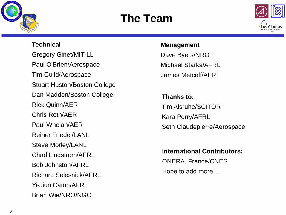
The Team

Technical

Gregory Ginet/MIT-LL

Paul O’Brien/Aerospace

Tim Guild/Aerospace

Stuart Huston/Boston College

Dan Madden/Boston College

Rick Quinn/AER

Chris Roth/AER

Paul Whelan/AER

Reiner Friedel/LANL

Steve Morley/LANL

Chad Lindstrom/AFRL

Bob Johnston/AFRL

Richard Selesnick/AFRL

Yi-Jiun Caton/AFRL

Brian Wie/NRO/NGC

Management

Dave Byers/NRO

Michael Starks/AFRL

James Metcalf/AFRL

International Contributors:

ONERA, France/CNES

Hope to add more…

Thanks to:

Tim Alsruhe/SCITOR

Kara Perry/AFRL

Seth Claudepierre/Aerospace

3

AP9/AE9 Program Objective

Provide satellite designers with a definitive model of the

trapped energetic particle & plasma environment

– Probability of occurrence (percentile levels) for flux and fluence

averaged over different exposure periods

– Broad energy ranges from keV plasma to GeV protons

– Complete spatial coverage with sufficient resolution

– Indications of uncertainty

L ~ Equatorial Radial Distance (RE)

HEO

GPS

GEO

0

50

100

150

200

250

CR

RE

S M

EP

-SE

U A

no

ma

lies

0

CR

RE

S V

TC

W A

no

ma

lies

5

10

15

1 2 3 4 5 6 7 8 0

10

20

30

SC

AT

HA

Surf

ace E

SD

SEUs

Internal

Charging

Surface

Charging

(Dose behind 82.5 mils Al)

SCATHA

Satellite Hazard Particle Population Natural Variation

Surface Charging 0.01 - 100 keV e- Minutes

Surface Dose 0.5 - 100 keV e-, H+, O+ Minutes

Internal Charging 100 keV - 10 MeV e- Hours

Total Ionizing Dose >100 keV H+, e- Hours

Single Event Effects >10 MeV/amu H+, Heavy ions Days

Displacement Damage >10 MeV H+, Secondary neutrons Days

Nuclear Activation >50 MeV H+, Secondary neutrons Weeks

Space particle populations and hazards

4

Requirements

Summary of SEEWG, NASA workshop & AE(P)-9 outreach efforts:

Priority Species Energy Location Sample Period Effects

1 Protons >10 MeV

(> 80 MeV)

LEO & MEO Mission Dose, SEE, DD,

nuclear activation

2 Electrons > 1 MeV LEO, MEO & GEO 5 min, 1 hr, 1 day,

1 week, & mission

Dose, internal charging

3 Plasma 30 eV – 100 keV

(30 eV – 5 keV)

LEO, MEO & GEO 5 min, 1 hr, 1 day,

1 week, & mission

Surface charging &

dose

4 Electrons 100 keV – 1 MeV MEO & GEO 5 min, 1 hr, 1 day,

1 week, & mission

Internal charging, dose

5 Protons

1 MeV – 10 MeV

(5 – 10 MeV)

LEO, MEO & GEO Mission Dose (e.g. solar cells)

(indicates especially desired or deficient region of current models)

Inputs:

• Orbital elements, start & end times

• Species & energies of concern (optional: incident direction of interest)

Outputs:

• Mean and percentile levels for whole mission or as a function of time for omni- or unidirectional,

differential or integral particle fluxes [#/(cm2 s) or #/(cm2 s MeV) or #/(cm2 s sr MeV) ] aggregated

over requested sample periods

5

L

Choose (E, K, ) coordinates

– IGRF/Olson-Pfitzer 77 Quiet B-field model

– Minimizes variation of distribution across magnetic epochs

( )m

m

s

m

s

K B B s ds

S

da B

2 2 2sin

2 2

p p

mB mB

2*

E

ML

R

Adiabatic invariants:

– Cyclotron motion:

– Bounce motion:

– Drift motion:

Coordinate System

K

or

L* and

K3

/4 (

RE-G

1/2

)3/4

(RE2

-G)

6

LEO Coordinate System

• Version Beta (, K) grid inadequate for LEO

– Not enough loss cone resolution

– No “longitude” or “altitude” coordinate

• Invariants destroyed by altitude-dependent density

effects

• Earth’s internal B field changes amplitude & moves

around

• What was once out of the loss-cone may no longer be

and vice-versa

• Drift loss cone electron fluxes cannot be neglected

–No systematic Solar Cycle Variation

60

80

100

120

140

160

180

200

220

F10.7

1975 1980 1985 1990 1995 2000 20050

0.5

1

1.5

2

2.5

3

3.5

Year

log

10(P

8 C

ount

Rate

)

Solar Cycle Variation at K1/4 = 0.5 -- vs. hmin

hmin

=200 km

hmin

=300 km

hmin

=400 km

hmin

=500 km

hmin

=600 km

hmin

=700 km

hmin

=800 km

• Version 1.0 will splice a LEO grid onto the (, K) grid at ~1000-2000 km

– Minimum mirror altitude coordinate hmin to replace

– Capture quasi-trapped fluxes by allowing hmin < 0 (electron drift loss cone)

7

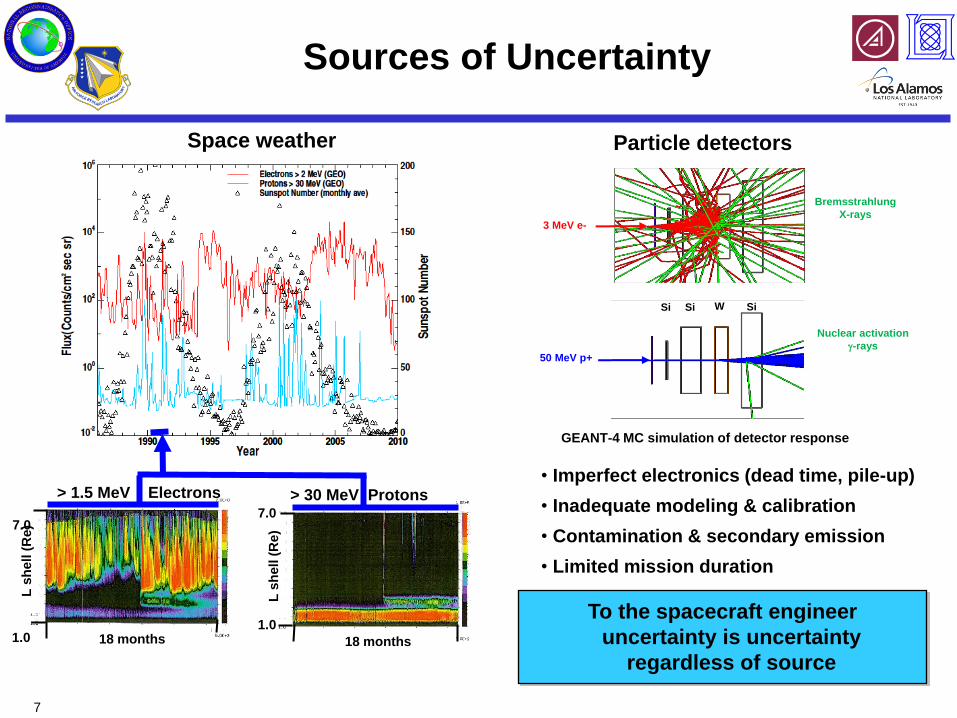
18 months 18 months

L s

he

ll (

Re

)

1.0

7.0

L s

he

ll (

Re

)

7.0

1.0

> 1.5 MeV Electrons > 30 MeV Protons

Particle detectors Space weather

Sources of Uncertainty

• Imperfect electronics (dead time, pile-up)

• Inadequate modeling & calibration

• Contamination & secondary emission

• Limited mission duration

Si Si W Si

3 MeV e-

50 MeV p+

GEANT-4 MC simulation of detector response

Bremsstrahlung

X-rays

Nuclear activation

-rays

To the spacecraft engineer

uncertainty is uncertainty

regardless of source

8

En

erg

y (

ke

V)

TEM1c PC-1 (45.12%)

keV

2 3 4 5 6 7 8

102

103

104

TEM1c PC-1 (45.12%)

2 3 4 5 6 7 8

102

103

104

TEM1c PC-2 (19.15%)

keV

2 3 4 5 6 7 8

102

103

104

TEM1c PC-2 (19.15%)

2 3 4 5 6 7 8

102

103

104

TEM1c PC-3 (9.36%)

keV

2 3 4 5 6 7 8

102

103

104

TEM1c PC-3 (9.36%)

2 3 4 5 6 7 8

102

103

104

TEM1c PC-4 (6.77%)

keV

L

2 3 4 5 6 7 8

102

103

104

z @ eq

=90o

-1 -0.5 0 0.5 1

TEM1c PC-4 (6.77%)

L

2 3 4 5 6 7 8

102

103

104

log10

Flux (#/cm2/sr/s/keV) @ eq

=90o

-4 -2 0 2 4 6Flux maps

• Derive from empirical data

• Create maps for median and 95th

percentile of distribution function

– Maps characterize nominal and extreme

environments

• Include error maps with instrument

uncertainty

• Apply interpolation algorithms to fill

in the gaps

Architecture Overview

18 months

L s

he

ll (

Re

)

1.0

7.0

Statistical Monte-Carlo Model

• Compute spatial and temporal correlation as

spatiotemporal covariance matrices

– From data (Version Beta & 1.0)

– Use one-day sampling time (Version Beta)

• Set up 1st order auto-regressive system to

evolve perturbed maps in time

– Covariance matrices gives SWx dynamics

– Flux maps perturbed with error estimate gives

instrument uncertainty

User application

• Runs statistical model N times

with different random seeds to get

N flux profiles

• Aggregates N profiles to get

median, 75th and 90th confidence

levels of flux & fluence

• Computes dose rate, dose or

other desired quantity derivable

from flux

Satellite data Satellite data & theory User’s orbit

+ = 50th

75th

95th

Mission time

Do

se

9

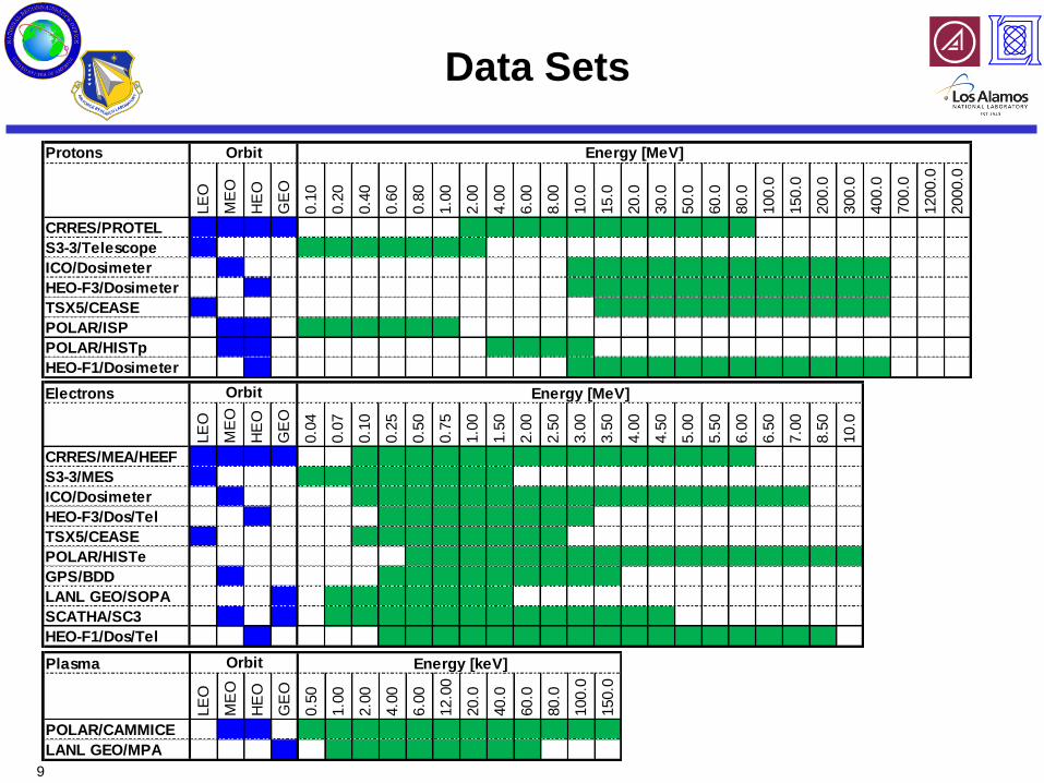
Protons

LE

O

ME

O

HE

O

GE

O

0.1

0

0.2

0

0.4

0

0.6

0

0.8

0

1.0

0

2.0

0

4.0

0

6.0

0

8.0

0

10.0

15.0

20.0

30.0

50.0

60.0

80.0

100.0

150.0

200.0

300.0

400.0

700.0

1200.0

2000.0

CRRES/PROTEL

S3-3/Telescope

ICO/Dosimeter

HEO-F3/Dosimeter

TSX5/CEASE

POLAR/ISP

POLAR/HISTp

HEO-F1/Dosimeter

Energy [MeV]Orbit

Data Sets

Electrons

LE

O

ME

O

HE

O

GE

O

0.0

4

0.0

7

0.1

0

0.2

5

0.5

0

0.7

5

1.0

0

1.5

0

2.0

0

2.5

0

3.0

0

3.5

0

4.0

0

4.5

0

5.0

0

5.5

0

6.0

0

6.5

0

7.0

0

8.5

0

10.0

CRRES/MEA/HEEF

S3-3/MES

ICO/Dosimeter

HEO-F3/Dos/Tel

TSX5/CEASE

POLAR/HISTe

GPS/BDD

LANL GEO/SOPA

SCATHA/SC3

HEO-F1/Dos/Tel

Energy [MeV]Orbit

Plasma

LE

O

ME

O

HE

O

GE

O

0.5

0

1.0

0

2.0

0

4.0

0

6.0

0

12.0

0

20.0

40.0

60.0

80.0

100.0

150.0

POLAR/CAMMICE

LANL GEO/MPA

Orbit Energy [keV]

10

Angle mapping to j90

Building Flux Maps

Low resolution energy & wide angle detector?

Sensor modeling Spectral inversion

Data collection Cross-calibration

Log Flux or Counts ( sat 1)

Lo

g F

lux

or

Co

un

ts (

sa

t 2

)

Binning to model grid

K3

/4

50 MeV protons

11

Example: Proton Flux Maps

Time history data

Flux maps (30 MeV)

•

F

j 90[#

/(cm

2 s

str

MeV

)]

j 90[#

/(cm

2 s

str

MeV

)]

•

•

Energy spectra

95th %

50th %

Year

j 90[#

/(cm

2 s

str

MeV

)]

Energy (MeV)

50th %

95th %

12

50th %

•

Example: Electron Flux Maps

Time history data

Flux maps (2.0 MeV)

j 90[#

/(cm

2 s

str

MeV

)]

Energy spectra

•

95th %

Year Energy (MeV)

j 90[#

/(cm

2 s

str

MeV

)]

50th %

95th %

13

Model Comparison: GPS Orbit

AE9 full Monte-Carlo – 40 runs Comparison of AE9 mean to AE8

Electrons > 1 MeV

14

Data Comparison: GEO electrons

DSP-21/CEASE (V.2)

0.125 MeV 1.25 MeV 0.55 MeV

10 year runs, 40 MC scenarios, 1 – 5 min time step

15

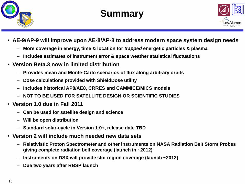
Summary

• AE-9/AP-9 will improve upon AE-8/AP-8 to address modern space system design needs

– More coverage in energy, time & location for trapped energetic particles & plasma

– Includes estimates of instrument error & space weather statistical fluctuations

• Version Beta.3 now in limited distribution

– Provides mean and Monte-Carlo scenarios of flux along arbitrary orbits

– Dose calculations provided with ShieldDose utility

– Includes historical AP8/AE8, CRRES and CAMMICE/MICS models

– NOT TO BE USED FOR SATELLITE DESIGN OR SCIENTIFIC STUDIES

• Version 1.0 due in Fall 2011

– Can be used for satellite design and science

– Will be open distribution

– Standard solar-cycle in Version 1.0+, release date TBD

• Version 2 will include much needed new data sets

– Relativistic Proton Spectrometer and other instruments on NASA Radiation Belt Storm Probes

giving complete radiation belt coverage (launch in ~2012)

– Instruments on DSX will provide slot region coverage (launch ~2012)

– Due two years after RBSP launch