appendix a: basic concepts from probability theory978-0-85729-647-4/1.pdf · appendix a: basic...

Appendix A: Basic Concepts fromProbability Theory

In this Appendix, we give a brief introduction to elementary probability theory,which is the basis of the mathematical approach to modeling failures. The presen-tation is non-rigorous. The objective is to develop an intuitive feel for the topicthat forms the foundation for most models used in solving reliability relatedproblems.

A.1 Scalar Random Variables

A scalar random variable X is useful in representing the outcome of an uncertainevent. It can be either discrete or continuous. A discrete random variable takes onat most a countable number of values (for example, the set of nonnegativeintegers) and a continuous random variable can take on values from a set ofpossible values which is uncountable (for example, values in the intervalð�1;1Þ).

Because the outcomes are uncertain, the value assumed by X is uncertain beforethe event occurs. Once the event occurs, X assumes a certain value. The standardconvention used is as follows: X (upper case) represents the random variablebefore the event and the value it assumes after the event is represented by x (lowercase).

A.1.1 Distribution and Density Functions

The distribution function F(x; h) is defined as the probability that X B x and isgiven by

Fðx; hÞ ¼ PfX� xg ðA:1Þ

W. R. Blischke et al., Warranty Data Collection and Analysis,Springer Series in Reliability Engineering, DOI: 10.1007/978-0-85729-647-4,� Springer-Verlag London Limited 2011

509

The domain of F(x; h) is ð�1;1Þ; the range is [0,1], and h denotes the set ofparameters of the distribution function. Often the parameters are omitted fornotational ease, so that one uses F(x) instead of F(x; h). We will do this in theremainder of the appendix.

F(x) has the following properties:

• F(x) is a non decreasing function in x.• Fð�1Þ ¼ 0 and Fð1Þ ¼ 1• For x1\x2 ; Pfx1\X� x2g ¼ Fðx2Þ � Fðx1Þ

When X is continuous valued and F(x) is differentiable, the density functionf(x) is given by

f ðxÞ ¼ dFðxÞdx

ðA:2Þ

f(x) may be interpreted as

Pfx\X� xþ dxg � f ðxÞdxþ Oðdx2Þ: ðA:3Þ

When X takes on only values in a set ðx1; x2; . . .; xnÞ; with n being finite orinfinite, the probability that X ¼ xi is given by

pi ¼ PfX ¼ xig; i ¼ 1; 2; . . .; n ðA:4Þ

In this case, X is called a discrete random variable, and the CDF is a step functionwith steps of height pi at each of the possible values xi.

1 pi has the followingproperties:

• pi C 0 is a non decreasing function in x.•Pn

i¼1 pi ¼ 1

A.1.1.1 Moments of Random Variables

The jth moment of the random variable X;MjðhÞ is given by2

MjðhÞ ¼ E½X j� ¼R1

0 x jf ðxÞdx; if X is continuousPx x jPfX ¼ xg; if X is discrete

�

ðA:5Þ

The first moment of X is called the mean and is usually denoted l, so that

510 Appendix A: Basic Concepts from Probability Theory

1 As before, the parameters may be omitted for notational ease, so that pi is often used instead ofpiðhÞ.2 The parameters are omitted for notational ease, so that one uses Mj instead of MjðhÞ. The sameis true for ljðhÞ.

l ¼ E½X� ðA:6Þ

The jth central moment of the random variable X, lj, is given by

lj ¼ E½ðX � lÞ j� ðA:7Þ

The second central moment of X is called the variance and is usually denoted r2,so that

r2 ¼ E½ðX � lÞ2� ðA:8Þ

r is called the standard deviation.

A.1.1.2 Fractiles of Distributions

For a continuous distribution, the a-fractile, xa, for a given a; 0\a\1; is anumber such that

PfX� xag ¼ FðxaÞ ¼ a ðA:9Þ

The fractiles for a = 0.25 and 0.75 are called first and third quartiles, respectively,of the distribution, and the 0.50-fractile is called the median.

A.1.2 Discrete Distributions

The following are some well known discrete distributions that are useful in failuremodeling3:Bernoulli Distribution Here X takes on two possible values, 0 and 1, withprobabilities given by

p0 ¼ p and p1 ¼ ð1� pÞ ðA:10Þ

The parameter set is h ¼ fpg; with 0� p� 1: The mean and variance are

l ¼ p and r2 ¼ pð1� pÞ ðA:11Þ

Binomial Distribution X assumes integer values from 0 to n, where n is a positiveinteger and pi; 0� i� n; is given by

pi ¼n!

i!ðn� iÞ! pið1� pÞðn�iÞ ðA:12Þ

Appendix A: Basic Concepts from Probability Theory 511

3 Most basic books on statistics and probability discuss some of the well-known distributions.References [14] and [15] give a more comprehensive coverage of many discrete distributions.

The parameter set is h ¼ fn; pg with 0� p� 1 and 0\n\1. The mean andvariance are

l ¼ np and r2 ¼ npð1� pÞ ðA:13Þ

Geometric Distribution X assumes integer values from 0 to ?, with probabilitiespi; 0� i\1, given by

pi ¼ ð1� pÞip ðA:14Þ

The parameter set is h ¼ fpg with 0� p� 1. The mean and variance are

l ¼ ð1� pÞp

and r2 ¼ ð1� pÞp2

ðA:15Þ

Hypergeometric Distribution X assumes integer values in the interval (max{0,n – N + D}, min{n, D}), where N, D and n are the three parameters of thedistribution, with N, D and n positive integers satisfying n�N and D B N. The pi

are given by

pi ¼ PðX ¼ iÞ ¼

Di

� �N � Dn� i

� �

Nn

� � ðA:16Þ

The mean and variance are given by

l ¼ nD

Nand VðXÞ ¼ ðN � nÞn

N � 1D

N

� �

1� D

N

� �

ðA:17Þ

Poisson Distribution X assumes integer values from 0 to ?. pi; 0� i\1; is givenby

pi ¼e�kki

i!ðA:18Þ

The parameter set is h ¼ fkg; with k[ 0. The mean and variance are given by

l ¼ k and r2 ¼ k ðA:19Þ

Multinomial Distribution This is an extension of the binomial distribution to thecase where there are k possible outcomes, with corresponding probabilities of

occurrence p1; p2; . . .; pk (withPk

i¼1 pi ¼ 1). The probability of observing ni itemsof type i ði ¼ 1; 2; . . .; kÞ in a sample of size n from an infinite population isgiven by

Pðn1; n2; . . .nkÞ ¼n!

n1!n2!. . .nk!pn1

1 pn22 . . .pnk

k ; ni� 0;Xk

i¼1

ni ¼ n; ðA:20Þ


A.1.3 Continuous Distribution and Density Functions

Some basic continuous distribution functions useful in failure modeling andstatistical analysis are the following4:

A.1.3.1 Basic Distributions and Density Functions

Exponential Distribution The distribution function for the exponential distributionis given by

Fðx; hÞ ¼ 1� e�kx; x� 0; ðA:21Þ

The parameter set is h = {k}, with k[ 0. The density function is

f ðx; hÞ ¼ ke�kx ðA:22Þ

The first two moments are given by

l ¼ 1k

and r2 ¼ 1

k2 ðA:23Þ

Gamma Distribution The gamma density function is given by

f ðx; hÞ ¼ xa�1e�x=b

baCðaÞ ; x� 0; ðA:24Þ

The parameter set is h ¼ fa; bg, with a[ 0 and b[ 0.The distribution and failure rate functions are complicated functions involving

confluent hyper-geometric functions [2]. The mean and variance are

l ¼ ab and r2 ¼ ab2 ðA:25Þ

Normal Gaussian Distribution The density function for the normal distribution isgiven by

f ðx; hÞ ¼ e�ðx�lÞ2=2r2

rffiffiffiffiffiffi2pp ; �1\x\1; ðA:26Þ

The parameter set is h ¼ fl; r2g, with r[ 0 and �1\l\1: It is not possibleto give analytical expressions for the distribution function. The mean and variance,l and r2; are also the parameters of the distribution.


4 Most basic books on statistics and probability discuss some of the well-known distributions.References [16, 17] give a more comprehensive coverage of many continuous distributions.

Uniform (Rectangular) Distribution The density function is given by

f ðx; hÞ ¼ 1b� a

; a� x� b: ðA:27Þ

The parameter set is h = {a, b}, with a \ b. The distribution function is given by

Fðx; hÞ ¼ x� a

b� aðA:28Þ

The mean and variance are

l ¼ ðaþ bÞ=2 and r2 ¼ ðb� aÞ2=12 ðA:29Þ

Weibull Distribution The two-parameter Weibull distribution function is given by

Fðx; hÞ ¼ 1� e�ðx=aÞb

; x� 0: ðA:30Þ

The parameter set is h = {a, b}, with a[ 0 and b[ 0. The failure densityfunction is given by

f ðx; hÞ ¼ bxðb�1Þe�ðx=aÞb

abðA:31Þ


l ¼ C 1þ 1b

� �

a and r2 ¼ C 1þ 2b

� �

� C 1þ 1b

� �� 2" #

a2 ðA:32Þ

Here Cð�Þ is the Gamma-function. Extensive table can be found in [2].Smallest Extreme Value Distribution The distribution function of smallest extremevalue (SEV) distribution is given by

Fðx; l; rÞ ¼ 1� exp �exp ðx� lÞ=rf g½ � ; �1\x\1: ðA:33Þ

The parameter set is h ¼ fl; rg; where l ð�1\l\1Þ is the location parameterand r[ 0 is the scale parameter. The density function is given by

f ðx; l; rÞ ¼ 1r

exp ðx� lÞ=r� exp ðx� lÞ=rf g½ � ; �1\x\1: ðA:34Þ


EðXÞ ¼ l� rc and VðXÞ ¼ r2p2

6ðA:35Þ

where c ¼ 0:5772 is Euler’s constant.It can be shown that the smallest extreme value distribution reduces to a

Weibull distribution (A.30) under the transformation

l ¼ lnðaÞ and r ¼ 1b

ðA:36Þ


Largest Extreme Value Distribution The distribution function of largest extremevalue (LEV) distribution is given by

Fðx; l; rÞ ¼ exp �exp �ðx� lÞ=rf g½ � ; �1\x\1: ðA:37Þ

The parameter set is h ¼ fl; rg; where l (�1\l\1) is a location parameterand r[ 0 is a scale parameter. The density function is given by

f ðx; l; rÞ ¼ 1r

exp �ðx� lÞ=r� exp �ðx� lÞ=rf g½ � ; �1\x\1: ðA:38Þ


EðXÞ ¼ lþ rc and VðXÞ ¼ r2p2

6ðA:39Þ

where c = 0.5772 is Euler’s constant.The smallest and largest extreme value distributions have a simple relationship.

If T � LEVðl; rÞ; then X ¼ �T � SEVð�l; rÞ:Fréchet Distribution The distribution function of the Fréchet distribution is

given by

Fðx; l; rÞ ¼ exp � l=xð Þr½ � ; x [ 0: ðA:40Þ

The parameter set is h ¼ fl; rg; where l[ 0 is a location parameter and r[ 0 isa scale parameter. The density function is given by

f ðx; l; rÞ ¼ rl

lx

� �rþ1exp � l=xð Þr½ � ; x [ 0: ðA:41Þ


EðXÞ ¼ C 1� 1r

� �

and VðXÞ ¼ C 1� 2r

� �

� C 1� 1r

� �� 2

ðA:42Þ

The mean and variance exist only if r[ 1 and r[ 2, respectively.

A.1.3.2 Derived Continuous Distribution and Density Functions

The derived distributions given below are obtained by (i) transformation of therandom variable from a basic distribution (for example, the log normaldistribution), (ii) modification of the form of a basic distribution by introducingadditional parameters (for example, the exponentiated Weibull distribution) and,(iii) devising forms that involve two or more basic distribution functions (forexample, mixtures of distribution, competing risk models). We present a few ofeach form of derived distribution.5


5 For additional details with regard to the three types, see [4, 34].

Inverse Gaussian (Wald) Distribution The density function is given by

f ðxÞ ¼ k2px3

� �1=2

exp�kðx� lÞ2

2l2x

!

; x [ 0: ðA:43Þ

The parameter set is h ¼ fl; kg; with l[ 0 and k[ 0: The mean is l and thevariance is l3=k:Lognormal Distribution The density function is given by

f ðx; hÞ ¼ e�fðlogðxÞ�lÞ2=2r2g

rxffiffiffiffiffiffi2pp ; x� 0: ðA:44Þ

The parameter set is h ¼ fl; rg with r[ 0 and �1\l\1: It is not possibleto give an analytical expression for the distribution function. The mean andvariance are

EðXÞ ¼ eðlþr2=2Þ and VðXÞ ¼ xðx� 1Þe2l ðA:45Þ

where x ¼ er2. The distribution is related to the normal in that if X is lognormal

(l, r), then Y = log(X) is N(l, r).Three Parameter Weibull Distribution This is an extension of the two-parameterWeibull distribution (A.30), given by

Fðx; hÞ ¼ 1� e�ðfx�sg=aÞb ; x� s: ðA:46Þ

The additional parameter is the location parameter s[ 0. The mean and varianceare given by

l ¼ sþ C 1þ 1b

� �

a and r2 ¼ C 1þ 2b

� �

� C 1þ 1b

� �� 2" #

a2 ðA:47Þ

Extended Weibull Distribution [29] The distribution function is given by

FðxÞ ¼ 1� me�ðx=aÞb

1� ð1� mÞe�ðx=aÞb; x� 0 ðA:48Þ

with 0� m� 1: The distribution reduces to the two-parameter Weibull (A.30) whenm = 1.Modified Weibull Distribution [21] The distribution function is given by

FðxÞ ¼ 1� expð�fx=agbemxÞ; x� 0; ðA:49Þ

with m C 0. The distribution reduces to the two-parameter Weibull (A.30) whenm = 0.


Exponentiated Weibull Distribution [32] The distribution function is given by

FðxÞ ¼ ½1� expf�ðx=aÞbg�m; x� 0; ðA:50Þ

with m C 0. The distribution reduces to the two-parameter Weibull (A.30) whenm = 1.Four parameter Weibull Distribution [19] The distribution function is given by

FðxÞ ¼ 1� exp �kx� a

b� x

� �b� �

; 0� a� x� b\1; ðA:51Þ

with k[ 0 and b[ 0. Note that the support is a finite interval.Mixtures of Distributions A finite mixture of distributions is a weighted average ofdistribution functions given by

FðxÞ ¼XK

i¼1

piFiðxÞ ðA:52Þ

with pi� 0; i ¼ 1; 2; . . .;K;PK

i¼1 pi ¼ 1 and FiðxÞ� 0; i ¼ 1; 2; . . .;K distributionfunctions (called the components of the mixture). If the components aredifferentiable, then the density function is given by

f ðxÞ ¼XK

i¼1

pifiðxÞ ðA:53Þ

Competing Risk The distribution function is given by

FðxÞ ¼ 1�YK

i¼1

ð1� FiðxÞÞ ðA:54Þ

The density function is

f ðxÞ ¼XK

i¼1

YK

k¼1k 6¼i

f1� FkðxÞg

2

664

3

775fiðxÞ ðA:55Þ

Multiplicative The distribution function is given by

FðxÞ ¼YK

i¼1

FiðxÞ; x� 0 ðA:56Þ

The density function is given by


f ðxÞ ¼XK

i¼1

YK

k¼1k 6¼i

FkðxÞfiðxÞ ðA:57Þ

A.1.3.3 Distributions of Importance in Statistical Inference

The following distributions are used extensively in data analysis. They areemployed in many important applications in estimation and hypothesis testing.Chi-Square Distribution The Chi-Square (v2) distribution is related to thedistribution of the sum of squares of normal random variables. The densityfunction is

f ðxÞ ¼ xðm�2Þ=2e�x=2

2m=2Cðm=2Þ ; x [ 0; ðA:58Þ

where Cð�Þ is the gamma function. The distribution function is an incompletegamma function [16]. The parameter is m, a positive integer called degrees offreedom. This density is a gamma distribution with shape parameter a ¼ m=2 andscale parameter b = 2. The mean is m and the variance is 2m.Student-t Distribution The density is

f ðxÞ ¼ C½ðmþ 1Þ=2�ffiffiffiffiffipmp

Cðm=2Þ½1þ x2=m�ðmþ1Þ=2; �1\x\1 ðA:59Þ

The parameter is m; m is a positive integer and is called degrees of freedom. TheCDF is a complex expression [17]. The mean is infinite if m = 1, and zero ifm C 2. The variance is infinite if m = 1 or 2 and m/(m - 2) if m[ 2.F Distribution The density function of the F distribution, also called the ‘‘varianceratio’’ or the ‘‘Fisher-Snedecor’’ distribution, is given by

f ðxÞ ¼ C½ðm1 þ m2Þ=2�ðm1=m2Þm1=2xðm1�2Þ=2

Cðm1=2ÞCðm2=2Þ½1þ m1x=m2�ðm1þm2Þ=2; x [ 0: ðA:60Þ

The parameter set is h ¼ fm1; m2g: Both parameters are positive integers calleddegrees of freedom. The mean is m2=ðm2 � 2Þ if m2 [ 2 and infinite otherwise. The

variance is infinite if m2� 4 and ½2m22ðm1 þ m2 � 2Þ�=½m1ðm2 � 2Þ2ðm2 � 4Þ� if m2 [ 4:

A.2 Two or More Random Variables

We first consider distributions in the case of two variables and then the generalcase of more than two.


A.2.1 Two Random Variables

We shall confine our discussion to two continuous random variables, denotedX and Y.

A.2.1.1 Joint, Marginal and Conditional Distributionand Density Functions

The joint distribution function F(x, y) is given by

Fðx; yÞ ¼ PfX� x; Y � yg ðA:61Þ

The random variables are said to be jointly continuous if there exists a functionf(x, y), called the joint probability density function, such that

f ðx; yÞ ¼ o2Fðx; yÞoxoy

ðA:62Þ

The marginal distribution functions FXðxÞ and FYðyÞ are given by

FXðxÞ ¼ Fðx;1Þ and FYðyÞ ¼ Fð1; yÞ ðA:63Þ

The two marginal density functions are given by

fXðxÞ ¼dFXðxÞ

dxand fYðyÞ ¼

dFYðyÞdy

: ðA:64Þ

The conditional distribution of X given that Y ¼ y is denoted F(x|y) and given by

FðxjyÞ ¼ PfX� xjY ¼ yg ðA:65Þ

The conditional distribution of Y given that X ¼ x ; Fðy xÞj , is defined similarly.For jointly continuous random variables with a joint density function f (x, y),

the conditional probability density function of X, given Y = y, is given by

f ðxjyÞ ¼ f ðx; yÞfYðyÞ

ðA:66Þ

Similarly,

f ðyjxÞ ¼ f ðx; yÞfXðxÞ

ðA:67Þ

The random variables X and Y are said to be independent (or statisticallyindependent) if and only if

Fðx; yÞ ¼ FXðxÞ FYðyÞ ðA:68Þ

for all x and y.


The results are similar for discrete random variables, with summation replacingintegration.

A.2.1.2 Moments of Two Random Variables

The covariance of X and Y is defined as

CovðX; YÞ ¼ E½fX � E½X�gfY � E½Y�g� ¼ E½X Y � � E½X� E½Y� ðA:69Þ

The correlation qXY is defined as

qXY ¼CovðX; YÞ

rXrY; ðA:70Þ

where rX and rY are the standard deviations of X and Y, respectively. The randomvariables X and Y are said to be uncorrelated if qXY ¼ 0: Note that independentrandom variables are uncorrelated but that the converse is not necessarily true.

A.2.1.3 Conditional Expectation

E½XjY ¼ y� is called the conditional expectation of X given that Y = y. Theunconditional expectation of X, given by

E½X� ¼Z1

�1

x fXðxÞ dx; ðA:71Þ

is related to the conditional expectation by the relation

E½X� ¼Z1

�1

E½XjY ¼ y� fYðyÞ dy: ðA:72Þ

This is written symbolically as

E½X� ¼ E½E½XjY�� ðA:73Þ

A.2.1.4 Bivariate Distribution and Density Functions

There are many multi-dimensional distributions.6 We list a few that are useful inreliability applications and data analysis.Bivariate Normal Distribution The joint distribution function is given by


6 Reference [18] discusses several multivariate distributions; Reference [12] deals with severalbivariate distributions.

Fðx;yÞ¼ 1

2prXrY

ffiffiffiffiffiffiffiffiffiffiffiffi1�q2

p

exp � 12ð1�q2Þ

x�lX

rX

� �2

�2qx�lX

rX

� �y�lY

rY

� �

þ y�lY

rY

� �2 !" #

ðA:74Þ

where q = qXY is the correlation coefficient and the remaining parameters are themeans and standard deviations of the marginal distributions of X and Y. Bothmarginal distributions are normal, as are the conditional distributions. In the lattercase, the means and standard deviations are functions of the condition [18].Bivariate Exponential Distributions A variety of bivariate exponential distributionshave been proposed in the literature. We list two of these.

1. Marshall and Olkin [29]

�Fðx; yÞ ¼ expf�½k1xþ k2yþ k12 maxðx; yÞ�g ðA:75Þ

where�Fðx; yÞ ¼ PfX [ x; Y [ yg ðA:76Þ

The marginal distributions are given by

FXðxÞ ¼ 1� expf�ðk1 þ k12Þxg ðA:77Þ

and

FYðyÞ ¼ 1� expf�ðk2 þ k12Þyg ðA:78Þ

respectively. It is easily shown that

PðX [ YÞ ¼ k2

k1 þ k2 þ k12; ðA:79Þ

PðX\YÞ ¼ k1

k1 þ k2 þ k12; ðA:80Þ

and

PðX ¼ YÞ ¼ k12

k1 þ k2 þ k12ðA:81Þ

2. Gumbel [9]

�Fðx; yÞ ¼ expð�x=h1Þ þ expð�y=h2Þ � expf�½ðx=h1Þm þ ðy=h2Þm�1=mg ðA:82Þ


7 See [34] for additional details on these as well as other bivariate Weibull distributions.

Bivariate Weibull Distributions A variety of bivariate Weibull distributions havebeen proposed in the literature. We list a few of these.7

1. Marshall and Olkin [29]

�Fðx; yÞ ¼ expf�½k1xb1 þ k2yb2 þ k12 maxðxb1 ; yb2Þ�g ðA:83Þ

2. Lee [23]

�Fðx; yÞ ¼ expf�½k1cb1xb þ k2cb

2yb þ k12 maxðcb1xb; cb

2ybÞ�g ðA:84Þ

3. Lu and Bhattacharyya [27]

�Fðx; yÞ ¼ expf�ðx=a1Þb1 � ðy=a2Þb2 � dhðx; yÞg ðA:85Þ

Different forms for the function of h(x, y) yield a family of models. Oneform for h(x, y) is the following:

hðx; yÞ ¼ ½ðx=a1Þb1=m þ ðy=a2Þb2=m�m ðA:86Þ

This results in

�Fðx; yÞ ¼ exp �ðx=a1Þb1 � ðy=a2Þb2 � d ðx=a1Þb1=m þ ðy=a2Þb2=mh imn o

ðA:87Þ

A.2.2 General Case

The k ([2) random variables may be represented by the vector ðX1;X2; . . .;XkÞ:The approach is similar to the two random variable case, but involving ank-dimensional distribution function Fðx1; x2; . . .; xkÞ: We have k marginaldistributions and several different conditional distributions, depending how thek-variables are divided into two sets, with the distribution of the first setconditioned on the values of the variables in the second. Similarly, there are manydifferent correlation coefficients. Details can be found in [18].


Appendix B: Introduction to Point Processes

One-dimensional [two-dimensional] point processes are useful for modelingrandom events involving warranty (e.g., number of warranty claims for productssold with 1-D [2-D] warranty). In this appendix, we discuss a few such processesand present some results (without proof) that will be used in the modeling andanalysis of warranties.8

B.1 One-dimensional Point Processes

A one-dimensional point process is a continuous-time stochastic process characterizedby events that occur randomly along the time continuum.

B.1.1 Counting Processes

A point process NðtÞ; t� 0f g is a counting process if it represents the number ofevents that have occurred until time t. It must satisfy:

• NðtÞ� 0:• N(t) integer valued.• If s \ t, then NðsÞ�NðtÞ• For s\t ; fNðtÞ � NðsÞg is the number of events in the interval (s,t].

It is assumed that Nð0Þ ¼ 0:

8 Proofs of the results can be found in many books on probability, for example, [43, 44]. Formore on point processes, see [6].


523

B.1.1.1 Non-Stationary Poisson Process

A counting process fNðtÞ; t� 0g is a non-stationary Poisson process if

• Nð0Þ ¼ 0:• fNðtÞ; t� 0g has independent increments.• PfNðt þ dtÞ � NðtÞ ¼ 1g ¼ kðtÞdt þ oðdtÞ:• PfNðt þ dtÞ � NðtÞ� 2g ¼ oðdtÞ:

k(t) is called the intensity function and is nonnegative. The function

KðtÞ ¼Z t

0

kðxÞ dx ðB:1Þ

is called the cumulative intensity function.Distribution and Moments of N(t) The probability that NðtÞ ¼ j is given by

pjðtÞ ¼ PfNðtÞ ¼ jg ¼ e�KðtÞfKðtÞg j

j!ðB:2Þ

for j� 0: The mean of N(t) is given by

MðtÞ ¼ E½NðtÞ� ¼ KðtÞ ðB:3Þ

The variance of N(t) is given by

V½NðtÞ� ¼ E½fNðtÞ � KðtÞg2� ¼ KðtÞ ðB:4Þ

Comment: If kðtÞ ¼ k; a constant, then the process is a stationary Poisson process.

B.1.1.2 Renewal Processes

A counting process fNðtÞ; t� 0g is an ordinary renewal process if

• Nð0Þ ¼ 0:• ~X1; the time to occurrence of the first event (counting from time t = 0) and

~Xj; j� 2; the time between the ðj� 1Þst and jth events, are a sequence ofindependent and identically distributed random variables with distributionfunction F(x).

• NðtÞ ¼ Sup fn : Sn� tg; where

S0 ¼ 0; Sn ¼Xn

i¼1

~Xi; n� 1 ðB:5Þ

524 Appendix B: Introduction to Point Processes

Distribution and Moments of N(t) The probability that N(t) = j is given by

pjðtÞ ¼ PfNðtÞ ¼ jg ¼ FðnÞðtÞ � Fðnþ1ÞðtÞ; ðB:6Þ

where FðnÞðtÞ is the n-fold convolution of F(t) with itself. This is obtained in arecursive manner as follows:

Fðjþ1ÞðtÞ ¼Z1

0

FðjÞðt � t0Þf ðt0Þdt0; ðB:7Þ

with Fð0ÞðtÞ ¼ 1:The expected value of NðtÞ; t� 0, denoted M(t), is given by

MðtÞ ¼X1

j¼1

FðjÞðtÞ ðB:8Þ

M(t) may also be obtained as the solution of the integral equation

MðtÞ ¼ FðtÞ þZ t

0

Mðt � xÞf ðxÞdx ðB:9Þ

This is called the renewal integral equation and M(t) is called the renewal functionassociated with the distribution function F(t).

The variance of NðtÞ; t� 0; is given by

VðtÞ ¼X1

n¼1

ð2n� 1ÞFðnÞðtÞ � ½MðtÞ�2: ðB:10Þ

For large t, an approximation of M(t) involving the first two moments of ~Xi isgiven by

MðtÞ � tlþ r2

ð2l2Þ � 1=2 ðB:11Þ

B.1.1.3 Delayed Renewal Process

A counting process fNðtÞ; t� 0g is a delayed renewal process if

• Nð0Þ ¼ 0.• ~X1, the time to the first event, is a non-negative random variable with

distribution function F(x).• ~Xj; j� 2; the time intervals between the jth and ðj� 1Þst events, are independent

and identically distributed random variables with a distribution functionF1(x) that is different from F(x).

• NðtÞ ¼ Sup fn : Sn� tg; where Sn is given by (B.5).

Appendix B: Introduction to Point Processes 525

Comment: When F1(x) equals F(x), the delayed renewal process reduces to anordinary renewal process.First Moment Md(t), the expected number of renewals over [0, t) for the delayedrenewal process, is given by

MdðtÞ ¼ FðtÞ þZ t

0

M1ðt � xÞ f ðxÞ dx ðB:12Þ

B.1.2 Mean Function of a Point Process

The mean function of a point process N(t), often referred to as the mean cumulativefunction (MCF), is defined as the expected value of N(t). This is given bylðtÞ ¼ E½NðtÞ�. If l(t) is differentiable, then

vðtÞ ¼ dE½NðtÞ�dt

¼ dlðtÞdt

ðB:13Þ

m(t) is called the recurrence rate or intensity function. In the context of reliability,where N(t) denotes the number of failures, it is also referred to as the rate ofoccurrence of failures (ROCOF).9

Comment: lðtÞ ¼ KðtÞ (given by (B.1)) in the case of a non-stationary Poissonprocess and lðtÞ ¼ MðtÞ (given by (B.8) or (B.9)) in the case of a renewal process.

B.1.3 Other Processes

B.1.3.1 Alternating Renewal Process

In an ordinary renewal process, the inter-event times are independent andidentically distributed. In an alternating renewal process, the inter-event times areindependent, but not identically distributed. More specifically, the odd numberedinter-event times (i.e., ~X1; ~X3; ~X5; . . .) are from a common distribution functionF(x) and the even numbered (i.e. ~X2; ~X4; ~X6; . . .) are from a common a distributionfunction G(x), that is different from F(x).

B.1.3.2 Marked Point Process

A marked point process is a point process with an auxiliary variable, called a mark,associated with each event. Let ~Yi; i� 1; denote the mark attached to the ith event.


9 For more details on MCF and ROCOF, see [42].

A simple marked point process is characterized by

• fNðtÞ; t� 0g; a stationary Poisson process with intensity k, and• a sequence of independent and identically distributed random variables f~Yig;

called marks, which are independent of the Poisson process.

B.1.3.3 Cumulative Process

A cumulative process, w(t), is given by

wðtÞ ¼XNðtÞ

i¼1

~Yi ðB:14Þ

with N(t) a marked point process and ~Yi the mark attached to event i. Thecumulative process is sometimes also called a compound Poisson process.

B.2 Two-dimensional Point Processes

Two-dimensional point processes deal with random events on a two-dimensionalplane, with one axis representing time and the other representing usage. In theensuing, ðTi;XiÞ; i� 1; denotes the time and usage of an item at the time at whichthe ith event occurs and T0 ¼ X0 ¼ 0: N t; xð Þ denotes the number of eventsoccurring over the interval ½0; tÞ ½0; xÞ:

B.2.1 Two-dimensional Renewal Processes

A two-dimensional renewal process is characterized by

• Nð0; 0Þ ¼ 0:• ð~Ti; ~XiÞ; i� 1; are a sequence of independent and identically distributed random

variables with bivariate distribution function F(t, x), where ~Ti ¼ Ti � Ti�1 and~Xi ¼ Xi � Xi�1; i� 1:

• Nðt; xÞ ¼ Sup fn : Tn� t;Xn� xg

Distribution and Moments10 The probability that Nðt; xÞ ¼ n is given by

pnðt; xÞ ¼ FðnÞðt; xÞ � Fðnþ1Þðt; xÞ; n� 0; ðB:15Þ

where FðnÞðt; xÞ is the n-fold bivariate convolution of F(t, x) with itself.

Appendix B: Introduction to Point Processes 527

10 For details, see [13].

The expected number of failures over ½0; tÞ ½0; xÞ is obtained by solution ofthe two-dimensional integral equation

Mðt; xÞ ¼ Fðt; xÞ þZ t

0

Zx

0

Mðt � u; x� vÞf ðu; vÞdvdu: ðB:16Þ


Appendix C: Probability Plots

In this appendix, we look at various theoretical and empirical plots. Whichempirical plot is appropriate in any given application depends on the type of dataavailable. These plots help in deciding whether or not a given data set can bemodeled by a specified distribution function. We first look at the empiricaldistribution function (EDF) plot. This does not involve a transformation of thedata. We then look at the WPP plot, which may be used to decide whether one ormore of the many Weibull-derived distributions can be used to model a given dataset. We conclude with a brief discussion of other probability plots.11

C.1 Types of Data

The types of data on which the plots are based may be (i) complete data,(ii) incomplete data, and (iii) grouped data.

• Complete Data: The data comprise solely the failure times for the n units and aregiven by the set ft1; t2; . . .; tng; where ti is the ith observation.

• Censored Data: The data consist of failure times of failed items and the ages ofunits that have not yet failed at the time of observation. For unit i, theobservation is the age at failure ti if the unit has failed and ~ti; the age of the unit,if it is still working.

• Grouped Data: The data available are not the failure times (as in the casecomplete data) but only the number of failures that occurred in different timeintervals. Let the number of observations in interval j; 1� j� J; be dj; with theinterval given by ½aj�1; ajÞ; where J is the number of intervals, a0 ¼ 0; and

aJ ¼ 1: Note that n ¼PJ

j¼1 dj:

11 We outline the procedures for other plots. For details, see [8, 22, 35].


529

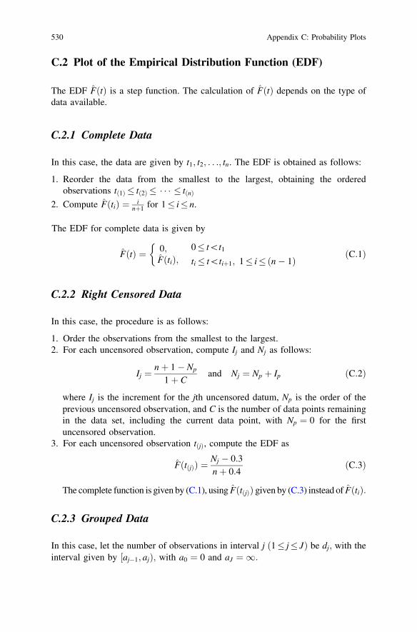
C.2 Plot of the Empirical Distribution Function (EDF)

The EDF FðtÞ is a step function. The calculation of FðtÞ depends on the type ofdata available.

C.2.1 Complete Data

In this case, the data are given by t1; t2; . . .; tn. The EDF is obtained as follows:

1. Reorder the data from the smallest to the largest, obtaining the orderedobservations tð1Þ � tð2Þ � � � � � tðnÞ

2. Compute FðtiÞ ¼ inþ1 for 1� i� n.

The EDF for complete data is given by

FðtÞ ¼ 0;FðtiÞ;

�0� t\t1

ti� t\tiþ1; 1� i�ðn� 1ÞðC:1Þ

C.2.2 Right Censored Data

In this case, the procedure is as follows:

1. Order the observations from the smallest to the largest.2. For each uncensored observation, compute Ij and Nj as follows:

Ij ¼nþ 1� Np

1þ Cand Nj ¼ Np þ Ip ðC:2Þ

where Ij is the increment for the jth uncensored datum, Np is the order of theprevious uncensored observation, and C is the number of data points remainingin the data set, including the current data point, with Np ¼ 0 for the firstuncensored observation.

3. For each uncensored observation tðjÞ, compute the EDF as

FðtðjÞÞ ¼Nj � 0:3nþ 0:4

ðC:3Þ

The complete function is given by (C.1), using FðtðjÞÞ given by (C.3) instead of FðtiÞ:

C.2.3 Grouped Data

In this case, let the number of observations in interval j ð1� j� JÞ be dj; with theinterval given by ½aj�1; ajÞ; with a0 ¼ 0 and aJ ¼ 1:

530 Appendix C: Probability Plots

The EDF is calculated as

FðajÞ ¼P j

i¼1 di

n; ðC:4Þ

with n ¼PJ

j¼1 dj:

C.3 WPP Plots

C.3.1 Theoretical Plot

For a failure distribution F(t), the Weibull transformation is given by

y ¼ logð�logð1� FðtÞÞÞ and x ¼ logðtÞ ðC:5Þ

A plot of y versus x is called the theoretical WPP Plot.12

The two-parameter Weibull distribution given by (A.30) is transformed into alinear relationship

y ¼ b½x� logðaÞ� ðC:6Þ

under the Weibull transformation. For other Weibull derived distributions, therelationship is non-linear. Murthy et al. [34] characterizes the different possibleshapes. These are listed in Table C.1

Table C.1 Classification of shapes for the WPP

Type Description

A Straight lineB ConcaveB1 Concave with left asymptote verticalC ConvexC1 Convex with right asymptote verticalD Single inflection point (S-shaped) with parallel asymptotesD1 Single inflection point (S-shaped) with vertical asymptotesE1 Bell shapedE(n) Multiple inflection points (n� 1 and odd)

Appendix C: Probability Plots 531

12 In the early 1970’s, a special paper was developed for plotting data under this transformation.The plotting paper was referred to as Weibull Probability Paper (WPP) and the plot called theWPP plot. At present, most computer reliability software packages and many statistical programpackages contain programs to produce these plots automatically, but the plot continues to becalled a WPP plot.

Shapes for the various Weibull-derived models discussed in Appendix A areindicated in Table C.2.13

C.3.2 Empirical WPP Plots

An empirical WPP plot is a plot on Weibull probability paper of an empiricaldistribution function (EDF) instead of the true distribution function. The procedurefor plotting the empirical WPP for various data sets is as follows:

C.3.2.1 Complete Data

The first two steps are as in Sect. C.2.1. The remaining steps are as follows:

3. Compute yi ¼ logð�logð1� FðtðiÞÞÞÞ for 1� i� n:4. Compute xi ¼ logðtðiÞÞ for 1� i� n:5. Plot yi versus xi for 1� i� n:

A smooth curve to fit the plotted data yields the empirical WPP Plot.

C.3.2.2 Right Censored Data

The first three steps are as in Sect. C.2.2. The remaining step is as follows:

4. Plot yj ¼ logð�logð1� FðtðjÞÞÞÞ versus xj ¼ logðtðjÞÞ for each uncensoredobservation.


Table C.2 Shapes of WPP Plots for various Weibull-derived distributions

Distributiona Shapes

Two-parameter Weilbull (A.30) AThree-parameter Weibull (A.46) B1Extended Weibull (A.48) B when m\1; C when m[ 1Modified Weibull (A.49) B when m[ 1; C when m\1Exponentiated Weibull (A.50) CFour-parameter Weibull (A.51) D1Mixture (A.52) with K ¼ 2 D when b1 ¼ b2; E(3) when b1 6¼ b2

Competing Risk (A.54) with K ¼ 2 CMultiplicative (A.56) with K ¼ 2 Ba The numbers refer to equation numbers in Appendix A


13 See [34] for details of the different shapes for other distributions that are either derived fromor linked to the Weibull distribution.

C.3.2.3 Grouped Data

The first step is as in Sect. C.2.3. The remaining step is as follows:

2. Plot yj ¼ logð�logð1� FðajÞÞÞ versus xj ¼ logðajÞ for 1� j� J:


C.3.3 Model Selection

The selection of a distribution to model a given data set based on WPP plotsinvolves comparing the empirical plot with each theoretical plot to see whether ornot the shapes of the two are similar. If the shapes are similar, the theoreticaldistribution is a candidate model. This issue is discussed further in [33, 34].

C.4 Other Plots

Plots have been proposed to determine if a given data set can be modeled bydistributions other than Weibull or Weibull-derived distributions. Many softwarepackages for reliability data modeling and statistical analysis have plots todetermine if a given data set can be modeled by an exponential, normal or log-normal distribution, and other distributions. We discuss the basis for the theoreticalplots of some of these below. The empirical plots follow along the lines indicatedin the above section, using the appropriate transformation.

C.4.1 Exponential Probability Plot

For a failure distribution F(t), the exponential probability plot is plot of y versusx under the transformation

y ¼ � logð1� FðtÞÞ and x ¼ t ðC:7Þ

If F(t) is the exponential distribution (given by (A.21)), then (C.7) reduces to astraight line given by

y ¼ kx ðC:8Þ

C.4.2 Normal Distribution Plot

For a failure distribution F(t), the normal probability plot is plot of y versus x underthe transformation


y ¼ F�1ðpÞ and x ¼ tp ðC:9Þ

If F(t) is the normal distribution (given by (A.26)), then (C.9) reduces to astraight line given by

x ¼ lþ ry ðC:10Þ

C.4.3 Lognormal Probability Plot

For a failure distribution F(t), the lognormal probability plot is plot of y versusx under the transformation

y ¼ U�1ðpÞ and x ¼ logðtpÞ; ðC:11Þ

where the function U�1ð�Þ is the inverse of the standard normal distributionfunction.

If F(t) is the lognormal distribution (given by (A.44)), then (C.11) reduces to astraight line given by


C.4.4 Smallest Extreme Value Probability Plot

For a failure distribution F(t), the smallest extreme value (SEV) probability plot isplot of y versus x under the transformation

y ¼ U�1sevðpÞ and x ¼ tp ðC:13Þ

where U�1sevðpÞ ¼ log½�logð1� pÞ�:

If F(t) is the smallest extreme value distribution (given by (A.33)), then (C.13)reduces to a straight line given by


C.4.5 Largest Extreme Value Probability Plot

For a failure distribution F(t), the largest extreme value (LEV) probability plot isplot of y versus x under the transformation

y ¼ U�1lev ðpÞ and x ¼ tp ðC:15Þ

where U�1lev ðpÞ ¼ �log½�logðpÞ�:


If F(t) is the largest extreme value distribution (given by (A.33)), then (C.15)reduces to a straight line given by

x ¼ �lþ ry ðC:16Þ

C.4.6 Fréchet Probability Plot

Taking natural logs twice of the Fréchet distribution function (A.40) yields a linearrelation in lnðtpÞ given by

�log½�logðpÞ� ¼ �r logðlÞ þ r logðtpÞ ðC:17Þ


Appendix D: Statistical Theory

In this appendix, we provide a brief introduction to some aspects of theoreticalstatistics that are important in understanding some of the topics covered in thetext. Included are comments on selected items from the theory of estimation, abrief development of maximum likelihood estimation, estimation of functions ofparameters, and use of the EM algorithm in analysis of incomplete data.

D.1 Estimation

D.1.1 Introduction

The objective of statistical inference generally is to use sample information tomake statements about populations. In estimation, the specific objective is toprovide methods of estimating (providing numerical values for) unknownpopulation parameters or other population characteristics. Implicit in thisapproach is that the form of the CDF14 is known or assumed. We considerestimation of a parameter h, which may be a scalar or vector parameter.

We also assume that the inference is to be based on a sample of n independentand identically distributed (iid) observations. These are indicated by capital lettersif they are considered to be random variables, with lower case used to indicate

numerical values. An estimator of a parameter h is a function h ¼ hðY1; . . . ; YnÞ;which is a random variable. A numerical value of the estimator, h ¼ hðy1; . . . ; ynÞ;is called an estimate. In general, a caret placed over a symbol will mean that thequantity is an estimator or an estimate. If it is not clear from the context which ofthese is meant, the more complete notation will be used.

14 See Appendix A for many examples of CDFs.


537

The remainder of this appendix will be devoted to a discussion of topics inestimation theory. The inference procedures discussed above are point estimatorsand estimates, and the derivation of these will be the focus of the discussion. Theseestimators are the basis of much of statistical inference, including confidenceinterval estimation, i.e., construction of a set of values along with a statement ofthe likelihood that the true value of the parameter is contained in the set, and therelated area of hypothesis testing.

Confidence intervals and other inferences may be based on exact results; theserequire knowledge of the exact distribution of the estimator. In many cases, it is notpossible to obtain this, but it is possible to obtain an asymptotic distribution, whichmay be used as the basis of, for example, an approximate confidence interval.

D.1.2 Approaches to Estimation

There are many approaches to the construction of estimators. A very commonly usedprocedure is maximum likelihood (ML). Maximum likelihood estimators (MLEs)are ‘‘best’’ in a number of senses. These will be discussed in the next sections.

Other methods of estimation15 include:

• Moment estimation: Express a set of k population moments in terms of thek unknown parameters. Solve the resulting equations to express the parametersin terms of the moments. Substitute sample moments for population moments.

• Least Squares (LS) estimation: Express the observations in terms of a model(often a linear model) involving the parameters. Sum the squares of deviationsof the observations from the model. LS estimators are those values thatminimize this expression.

• Bayes estimation: Determine a prior distribution of the parameters. Express thejoint distribution of the data in terms of this and the assumed distribution of theobservations. Use Bayes’ Theorem to determine a posterior distribution and basethe estimator on this.

• Minimum Chi-Square estimation: Form a Chi-Square statistic based on thedifference between the observations (often grouped) and a model. Theestimators are those values that minimize this quantity.

• Best Asymptotically Normal (BAN) estimation: A large class of estimators thatare asymptotically normally distributed. If certain conditions are met, the MLE,minimum Chi-Square, and LS estimators are BAN.

538 Appendix D: Statistical Theory

15 See books on theoretical statistics such as [5, 11, 24, 46] for details on these and othermethods.

D.1.3 Properties of Estimators

In practice, it is necessary to choose among the many possible estimators. This isdone on the base of how they perform when applied to the many data sets that mayoccur. The objective is to use a ‘‘best’’ procedure, i.e., one that is optimal in one ormore senses. Criteria of optimality in this context include the following16:

Sufficiency An estimator h is sufficient if the conditional distribution of Y1,

Y2, … , Yn given h does not depend on h. This implies that h contains all of thesample information about h.

Unbiasedness An estimator h is unbiased if EðhÞ ¼ h; for all values of h.

Asymptotic unbiasedness An estimator h is asymptotically unbiased if

EðhÞ ! h; as n!1; for all values of h.

Consistency An estimator h is consistent if for all h, Pðjh� hj[ eÞ ! 0 asn!1 for any e [ 0.

Efficiency An estimator is efficient within a class of estimators (e.g., unbiased) ifno other estimator in the class has smaller variance.

Asymptotic efficiency An estimator is asymptotically efficient if it is efficient asn ? ?.

There are many other such criteria. See [4] and the references cited. All of theabove and some others are desirable properties of estimators. It is very rare,however, that an estimator can be found that satisfies all, or even many, of theoptimality criteria.

An important result that is useful in evaluating estimators is the Cramér-RaoInequality, which gives a lower bound on the variance of any unbiased estimator.The result is as follow:

Cramér-Rao Inequality Suppose that T ¼ T Y1; Y2; . . . ; Ynð Þ is an unbiasedestimator of a function sðhÞ; with k = 1. Then under certain regularity conditionson s and the distribution of Y1; Y2; . . . ; Yn [46],

VðTÞ� ½s0ðhÞ�2

E o log½LðY1;... ;Yn;h�oh

n o2 ðD:1Þ

for all h, where

LðY1; . . . ; Yn; hÞ ¼Yn

i¼1

f ðYi; hÞ ðD:2Þ

Appendix D: Statistical Theory 539

16 Note that the definitions given are not completely rigorous, but are intended to give the readera sense of these criteria. For mathematically precise definitions see books on theoretical statisticssuch as [5, 11, 46].

The denominator of (D.1) is known as the Fisher Information, and is denotedI(h). If sðhÞ ¼ h; the lower bound on the variance of an unbiased estimator is 1/I(h).

If the variance of an estimator achieves this bound, it is an efficient, unbiasedestimator. If it achieves the bound as n ? ?, the estimator is asymptoticallyefficient.

If an estimator h of h is biased, with bias given by bðhÞ ¼ EðhÞ � h; the boundbecomes

VðhÞ� ½1þ b0ðhÞ�2

IðhÞ ðD:3Þ

For k[1, the results extend to bounds on the covariance matrix of a vector ofestimators of the elements of h. The bounds are based on the k k Fisherinformation matrix, with elements

Iij ¼ Eo

ohilog½f ðy; hÞ� o

ohjlog½f ðy; hÞ�

� �

ðD:4Þ

See the references on theoretical statistics cited above for additional details.

D.2 Method of Maximum Likelihood

D.2.1 Complete Data

The maximum likelihood estimator (MLE) is obtained by maximizing thelikelihood function, which is defined to be the joint distribution of theobservations in a random sample. The likelihood function is given in (D.2) forcomplete data. For ease of computation, we ordinarily maximize the natural log ofthe likelihood function.17 Maximization is with regard to the components of h, and,under the assumption of differentiability, is accomplished by equating thederivatives to zero and solving the resulting likelihood equations. If necessary, theML equations may be solved by numerical methods. Solutions for a number of lifedistributions are given in most statistical packages.

The rationale for use of the MLE is the Maximum Likelihood Principle, whichessentially states that one should choose as an estimator the values of theparameters that make the data actually observed most likely to have occurred.In practice, the MLE is used because it is optimal in many ways.

The optimality of the MLE depends on certain regularity conditions. These are:(1) the first two derivatives of the log-likelihood with respect to the components of


17 Thus we deal with a sum, and the resulting equations are simpler. Since log is a one-to-onefunction, the solutions are identical.

h must be defined; and (2) I(h) must not be zero and must be a continuous of thecomponents of h. Under these conditions, the MLEs are consistent, asymptoticallyunbiased, asymptotically efficient, and asymptotically normally distributed.

These results apply to incomplete as well as complete data. In the next twosections we look at the likelihood functions for censored data and grouped data.

D.2.2 Censored Data

The likelihood function for censored data depends on the type of censoring.We consider the types ordinarily found in reliability and warranty claims data.

Type I censoring Censoring as a function of time is called Type I censoring.We are concerned with right censoring. In reliability testing, this occurs whentesting is stopped at a specified time T. For claims data, censoring occurs at the endof the warranty period, i.e., at T = W.

Suppose that all n items are put on test or sold at time 0 and that r items havefailed by time T. The data may be written as ordered observations, in which casethey consist of failure times for the first r items, say Y1, … , Yr, and the value T forthe remaining (censored) items. The likelihood function is

LðY1; . . . ; Yn; hÞ ¼Yr

i¼1

f ðYiÞ( )

½1� FðT; hÞ�n�r ðD:5Þ

Note that here r is a random variable. The implication of this is that maximizationmay not be approached simply by differentiation of the likelihood or log-likelihood, and alternate methods, e.g., search routines, are required.

In practice, warranty claims data are often multiply censored. This occurs inwarranty data when items are sold at different times. In this case, the likelihoodfunction becomes

LðY1; . . . ; Yn; hÞ ¼Yr

i¼1

f ðYiÞYn

i¼rþ1

½FðW ; hÞ � FðYi; hÞ� ðD:6Þ

where Yr+1, …, Yn are the times of sale of the unfailed items.Type II censoring Testing continues until a predetermined number r of failures

occur. The data are as above. The likelihood function is

LðY1; . . . ; Yn; hÞ ¼Yr

i¼1

f ðYiÞYn

i¼rþ1

½1� FðYi; hÞ� ðD:7Þ

The MLEs are obtained by minimization of (D.7). The properties of the MLEsare as indicated above. For additional results, including the likelihood function forother types of censoring, see [30].


D.2.3 Grouped Data

We assume that the observations are grouped into k intervals defined by endpointsy00; y

01; . . . ; y0k: The number of observations falling into the ith interval is ni, where

Pki¼1 ni ¼ n: The likelihood function is given by

Lðn1; . . . ; nk; hÞ ¼n!

n1! . . . nk!

Yk

i¼1

½Fðy0i; hÞ � Fðy0i�1; hÞ�ni ðD:8Þ

For data that are censored as well as grouped, the likelihood function ismodified as in (D.6). Let ri denote the number of observations censored at ithinterval. The likelihood function can be written as

LðhÞ /Yk

i¼1

½Fðy0i; hÞ � Fðy0i�1; hÞ�ni ½1� Fðy0i; hÞ�ri ðD:9Þ

D.2.4 Asymptotic Confidence Intervals and Tests

The asymptotic normality of the MLEs may be used to obtain asymptoticconfidence intervals and asymptotic test of hypotheses. Asymptotic variances andcovariances of the estimators are obtained as the elements of the inverse of theinformation matrix with elements given by (D.4). These may be estimated bysubstituting MLEs of the parameters involved. The confidence intervals and testsare then done by use of the procedures based on the normal distribution.

D.3 Estimation of Functions of Random Variables

In reliability and warranty analyses, we often encounter problems in whichestimators of functions of parameters are needed. Here we look briefly at someapproaches to problems of this type and illustrate the methodology by consideringsums, products and ratios of random variables. Most of the results given areasymptotic results. These provide the means of obtaining asymptotic confidenceintervals and tests.

D.3.1 Asymptotic Mean and Variance of a Function

Assume that Y is a random variable with mean l and finite variance V(Y) and lets(Y) be a twice-differentiable function of Y. Then


E½sðYÞ� � sðlÞ þ 0:5 s00ðlÞVðYÞ ðD:10Þ

and

VððsðYÞÞ � ½s0ðlÞ�2VðYÞ: ðD:11Þ

In practice, only the first-order approximation of the expectation is used, in whichcase the result is E½sðYÞ� � sðlÞ:

This extends to k random variables as follows: Let Y1, Y2, …, Yk be randomvariables with respective means li, variances r2

i ¼ V Yið Þ and covariancesrij ¼ Cov Yi; Yj

�¼ E Yi � lið Þ Yj � lj

�� , and let s Y1; Y2; . . . ; Ykð Þ be a function

such that all second-order derivatives exist. Then

E½sðYl; . . . ; YkÞ� � sðll; . . .; lkÞ þXk

i¼1

r2i

o2soY2

i

� ��ll;...;lk

þ 2X

i\j

rijo2s

oYioYj

� ��ll;...;lk

ðD:12Þ

and

VðsðYi; . . .; YkÞÞ �Xk

i¼1

r2i

osoYi

� �2��l1;...;lk

þ 2X

i\j

rijosoYi

� �osoYj

� ��l1;...;lk

ðD:13Þ

Again, in practice only the first order approximation to the expectation is used.It was noted above that the MLE is asymptotically normally distributed. Under

fairly general conditions, this is true of functions of the MLE as well, with meansand variances are given in (D.10–D.13). It follows that asymptotic confidenceintervals and tests may be constructed based on these results. These are appropriatefor large n and are obtained by substitution of MLE’s into the formulas for theasymptotic variance and use of fractiles of the standard normal distribution.

D.3.2 Sums of Random Variables

Assume that Y1; Y2; . . . ; Yn are random variables with respective means li andfinite variances ri

2 and covariances rij. Let c0; c1; . . . ; cn be a sequence of constantsand Y ¼ c0 þ

Pni¼1 ciYi: Then the mean and variance of Y are given by

EðYÞ ¼ c0 þXn

i¼1

cili ðD:14Þ

and

VðYÞ ¼Xn

i¼1

c2i r

2i þ 2

X

i\j

cicjrij: ðD:15Þ


It follows from these results that if the Yi’s are independent and identicallydistributed, then the sample mean �Y has expectation l and variance r2/n. Anotherimportant result is that if, in addition, the Yi’s are normally distributed, then �Y isalso normal. Finally, by the Central Limit Theorem, under fairly generalconditions �Y is asymptotically normally distributed.

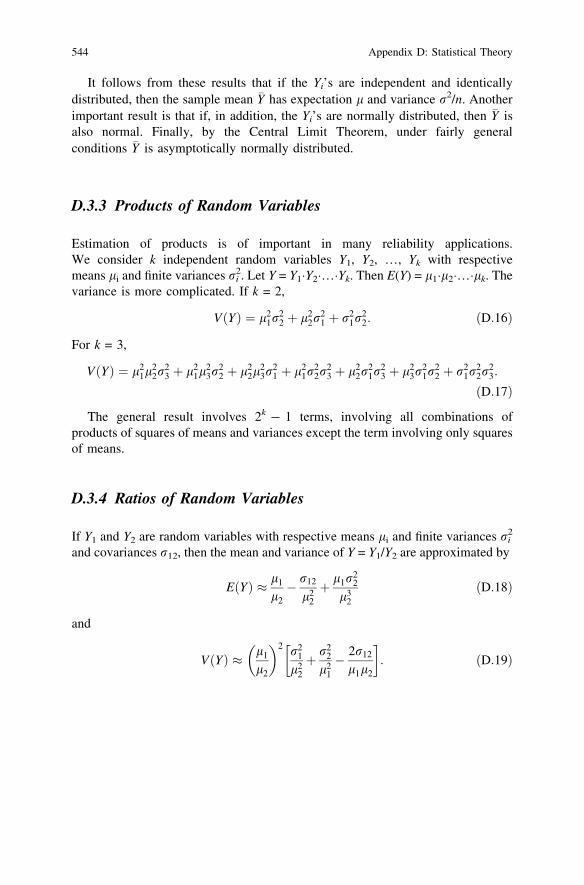
D.3.3 Products of Random Variables

Estimation of products is of important in many reliability applications.We consider k independent random variables Y1, Y2, …, Yk with respectivemeans li and finite variances ri

2. Let Y = Y1�Y2�…�Yk. Then E(Y) = l1�l2�…�lk. Thevariance is more complicated. If k = 2,

VðYÞ ¼ l21r

22 þ l2

2r21 þ r2

1r22: ðD:16Þ

For k = 3,

VðYÞ ¼ l21l

22r

23 þ l2

1l23r

22 þ l2

2l23r

21 þ l2

1r22r

23 þ l2

2r21r

23 þ l2

3r21r

22 þ r2

1r22r

23:

ðD:17Þ

The general result involves 2k - 1 terms, involving all combinations ofproducts of squares of means and variances except the term involving only squaresof means.

D.3.4 Ratios of Random Variables

If Y1 and Y2 are random variables with respective means li and finite variances ri2

and covariances r12, then the mean and variance of Y = Y1/Y2 are approximated by

EðYÞ � l1

l2� r12

l22

þ l1r22

l32

ðD:18Þ

and

VðYÞ � l1

l2

� �2 r21

l22

þ r22

l21

� 2r12

l1l2

� �

: ðD:19Þ


D.4 MLE for Incomplete Data using the EM Algorithm

The Expectation-Maximization (EM) algorithm is a broadly applicable iterativeprocedure for computing maximum likelihood estimates in problems withincomplete data. The EM algorithm consists of two conceptually distinct stepsat each iteration: the expectation or E-step and the maximization or M-step.18

Suppose we have a model for a set of complete data Y, with associated densityf ðY jhÞ; where h ¼ ðh1; h2; . . .; hdÞ0 is a vector of unknown parameters withparameter space X We write Y ¼ ðYobs; YmisÞ where Yobs represent the observedpart of Y and Ymis denotes the missing values. The EM algorithm is designed to findthe value the value of h, denoted h; that maximizes the incomplete data log-likelihood log LðhÞ ¼ log f ðYobsjhÞ; that is, the MLE of h based on the observeddata Yobs:

The EM algorithm starts with an initial value hð0Þ 2 X: Suppose that hðkÞ

denotes the estimate of h at the kth iteration; then the (k ? 1)st iteration can bedescribed in two steps as follows:

E-step: Find the conditional expected complete-data log-likelihood given

observed data and h ¼ hðkÞ:

QðhjhkÞ ¼ Eðlog LðY jYobs; h ¼ hðkÞÞÞ

¼Z

log LðhjYÞf ðYmisjYobs; h ¼ hkÞdYmis ðD:20Þ

which, in the case of linear exponential family, amounts to estimating the sufficientstatistics for the complete data.

M-step: Determine hðkþ1Þ to be a value of h 2 X that maximizes QðhjhðkÞÞ:The MLE of h is found by iterating between the E and M steps until a

convergence criterion is met. In some cases, it may not be numerically feasible to

find the value of h that globally maximizes the function QðhjhðkÞÞ in the M-step. In

such situations, a Generalized EM (GEM) algorithm [7] is used to choose hðkþ1Þ inthe M-step such that the condition

Qðhðkþ1ÞjhðkÞÞ �QðhðkÞjhðkÞÞ ðD:21Þ

holds. For any EM or GEM algorithm, the change from hðkÞ to hðkþ1Þ increases thelikelihood; that is,

log Lðhðkþ1ÞÞ � log LðhðkÞÞ ðD:22Þ

which follows from the definition of GEM and Jensen’s inequality.19 This factimplies that the log-likelihood, log L(h), increases monotonically on any iteration

18 For details, see [7, 10, 25, 28].19 See p. 47 of [40].


sequence generated by the EM algorithm, which is the fundamental property forthe convergence of the algorithm.20 Meng and Rubin [31], Louis [26] and Oakes[38] derived methods for obtaining the asymptotic variance-covariance matrix ofthe EM-computed estimator.


20 Detailed properties of the algorithm, including the convergence properties, are given in [7, 28,41, 48].

Appendix E: Statistical Tables

Percentiles of statistical distributions and related tables are needed for manypurposes in statistical inference. Even though most, if not all, of these can beobtained on-line or from statistical program packages, it is often useful to havethe tables at hand in books such as this. We provide the following statisticaltables:

E.1 Fractiles zp of the standard normal distributionE.2 Fractiles of the Student-t distributionE.3 Fractiles of the Chi-Square distribution shapes.E.4 Fractiles of the F distributionE.5 Factors for two-sided normal tolerance limitsE.6 Factors for one-sided normal tolerance limitsE.7 Factors for two-sided nonparametric tolerance limits

Table E.1 Fractiles zp of the Standard Normal Distribution. (P(Z B zp) = p)

p zp p zp

0.0005 -3.291 0.8000 0.8420.0010 -3.091 0.8500 1.0360.0025 -2.807 0.9000 1.2820.0050 -2.576 0.9500 1.6450.0100 -2.326 0.9750 1.9600.0200 -2.054 0.9800 2.0540.0250 -1.960 0.9900 2.3260.0500 -1.645 0.9950 2.5760.1000 -1.282 0.9975 2.8070.1500 -1.036 0.9990 3.0910.2000 -0.842 0.9995 3.291


547

Table E.2 Fractiles of the Student-t distribution

df p

0.900 0.950 0.975 0.990 0.995

1 3.078 6.314 12.706 31.821 63.6572 1.886 2.920 4.303 6.965 9.9253 1.638 2.353 3.182 4.541 5.8414 1.533 2.132 2.776 3.747 4.6045 1.476 2.015 2.571 3.365 4.0326 1.440 1.943 2.447 3.143 3.7077 1.415 1.895 1.365 2.998 3.4998 1.397 1.860 2.306 2.896 2.3559 1.383 1.833 2.262 2.821 3.25010 1.372 1.812 2.228 2.764 3.16911 1.363 1.796 2.201 2.718 3.10612 1.356 1.782 2.179 2.681 3.05513 1.350 1.771 2.160 2.650 3.01214 1.345 1.761 2.145 2.624 2.97715 1.341 1.753 2.131 2.602 2.94716 1.337 1.746 2.120 2.583 2.92117 1.333 1.740 2.110 2.567 2.89818 1.330 1.734 2.101 2.552 2.87819 1.328 1.729 2.093 2.539 2.86120 1.325 1.725 2.086 2.528 2.84521 1.323 1.721 2.080 2.518 2.83122 1.321 1.717 2.074 2.508 2.81923 1.319 1.714 2.069 2.500 2.80724 1.318 1.711 2.064 2.492 2.79725 1.316 1.708 2.060 2.485 1.78726 1.315 1.706 2.056 2.479 2.77927 1.314 1.703 2.052 2.473 2.77128 1.313 1.701 2.048 2.467 2.76329 1.311 1.699 2.045 2.462 2.75630 1.310 1.697 2.042 2.457 2.75035 1.306 1.690 2.030 2.438 2.71540 1.303 1.684 2.021 2.423 2.70445 1.301 1.679 2.014 2.412 2.69050 1.299 1.676 2.009 2.403 2.67855 1.297 1.673 2.004 2.396 2.66860 1.296 1.671 2.000 2.390 2.66065 1.295 2.669 1.997 2.385 2.65470 1.294 1.667 1.994 2.381 2.64875 1.293 2.665 1.992 2.377 2.64380 1.292 1.664 1.990 2.374 2.63985 1.292 1.663 1.988 2.371 2.63590 1.291 1.662 1.987 2.369 2.63295 1.291 1.661 1.985 2.366 2.629100 1.290 1.660 1.984 2.364 2.626200 1.286 1.653 1.972 2.345 2.601500 1.283 1.648 1.965 2.334 2.586? 1.282 1.645 1.960 2.326 2.576

548 Appendix E: Statistical Tables

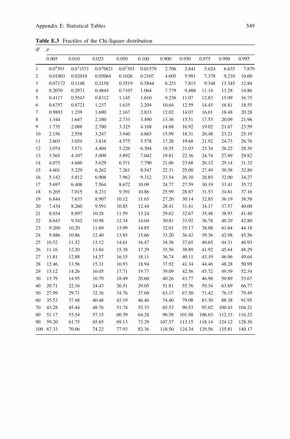
Table E.3 Fractiles of the Chi-Square distribution

df p

0.005 0.010 0.025 0.050 0.100 0.900 0.950 0.975 0.990 0.995

1 0.04393 0.031571 0.039821 0.02393 0.01579 2.706 3.841 5.024 6.635 7.879

2 0.01003 0.02010 0.05064 0.1026 0.2107 4.605 5.991 7.378 9.210 10.60

3 0.07172 0.1148 0.2158 0.3519 0.5844 6.251 7.815 9.348 11.345 12.84

4 0.2070 0.2971 0.4844 0.7107 1.064 7.779 9.488 11.14 13.28 14.86

5 0.4117 0.5543 0.8312 1.145 1.610 9.236 11.07 12.83 15.09 16.75

6 0.6757 0.8721 1.237 1.635 2.204 10.64 12.59 14.45 16.81 18.55

7 0.9893 1.239 1.690 2.167 2.833 12.02 14.07 16.01 18.48 20.28

8 1.344 1.647 2.180 2.733 3.490 13.36 15.51 17.53 20.09 21.96

9 1.735 2.088 2.700 3.325 4.168 14.68 16.92 19.02 21.67 23.59

10 2.156 2.558 3.247 3.940 4.865 15.99 18.31 20.48 23.21 25.19

11 2.603 3.054 3.816 4.575 5.578 17.28 19.68 21.92 24.73 26.76

12 3.074 3.571 4.404 5.226 6.304 18.55 21.03 23.34 26.22 28.30

13 3.565 4.107 5.009 5.892 7.042 19.81 22.36 24.74 27.69 29.82

14 4.075 4.660 5.629 6.571 7.790 21.06 23.68 26.12 29.14 31.32

15 4.601 5.229 6.262 7.261 8.547 22.31 25.00 27.49 30.58 32.80

16 5.142 5.812 6.908 7.962 9.312 23.54 26.30 28.85 32.00 34.27

17 5.697 6.408 7.564 8.672 10.09 24.77 27.59 30.19 33.41 35.72

18 6.265 7.015 8.231 9.391 10.86 25.99 28.87 31.53 34.81 37.16

19 6.844 7.633 8.907 10.12 11.65 27.20 30.14 32.85 36.19 38.58

20 7.434 8.260 9.591 10.85 12.44 28.41 31.41 34.17 37.57 40.00

21 8.034 8.897 10.28 11.59 13.24 29.62 32.67 35.48 38.93 41.40

22 8.643 9.542 10.98 12.34 14.04 30.81 33.92 36.78 40.29 42.80

23 9.260 10.20 11.69 13.09 14.85 32.01 35.17 38.08 41.64 44.18

24 9.886 10.86 12.40 13.85 15.66 33.20 36.42 39.36 42.98 45.56

25 10.52 11.52 13.12 14.61 16.47 34.38 37.65 40.65 44.31 46.93

26 11.16 12.20 13.84 15.38 17.29 35.56 38.89 41.92 45.64 48.29

27 11.81 12.88 14.57 16.15 18.11 36.74 40.11 43.19 46.96 49.64

28 12.46 13.56 15.31 16.93 18.94 37.92 41.34 44.46 48.28 50.99

29 13.12 14.26 16.05 17.71 19.77 39.09 42.56 45.72 49.59 52.34

30 13.79 14.95 16.79 18.49 20.60 40.26 43.77 46.98 50.89 53.67

40 20.71 22.16 24.43 26.51 29.05 51.81 55.76 59.34 63.69 66.77

50 27.99 29.71 32.36 34.76 37.69 63.17 67.50 71.42 76.15 79.49

60 35.53 37.48 40.48 43.19 46.46 74.40 79.08 83.30 88.38 91.95

70 43.28 45.44 48.76 51.74 55.33 85.53 90.53 95.02 100.43 104.21

80 51.17 53.54 57.15 60.39 64.28 96.58 101.88 106.63 112.33 116.32

90 59.20 61.75 65.65 69.13 73.29 107.57 113.15 118.14 124.12 128.30

100 67.33 70.06 74.22 77.93 82.36 118.50 124.34 129.56 135.81 140.17

Appendix E: Statistical Tables 549

Table E.4 F distribution (p = upper-tail probability, n1: denominator df; n2: numerator df).

n2 p n1

1 2 3 4 5 6 7 8 9 10

0.10 4.06 3.78 3.62 3.52 3.45 3.40 3.37 3.34 3.32 3.305 0.05 6.61 5.79 5.41 5.19 5.05 4.95 4.88 4.82 4.77 4.74

0.01 16.26 13.27 12.06 11.39 10.97 10.67 10.46 10.29 10.16 10.050.10 3.78 3.46 3.29 3.18 3.11 3.05 3.01 2.98 2.96 2.94

6 0.05 5.99 5.14 4.76 4.53 4.39 4.28 4.21 4.15 4.10 4.060.01 13.75 10.92 9.78 9.15 8.75 8.47 8.26 8.10 7.98 7.870.10 3.59 3.26 3.07 2.96 2.88 2.83 2.78 2.75 2.72 2.70

7 0.05 5.59 4.74 4.35 4.12 3.97 3.87 3.79 3.73 3.68 3.640.01 12.25 9.55 8.45 7.85 7.46 7.19 6.99 6.84 6.72 6.620.10 3.46 3.11 2.92 2.81 2.73 2.67 2.62 2.59 2.56 2.54

8 0.05 5.32 4.46 4.07 3.84 3.69 3.58 3.50 3.44 3.39 3.350.01 11.26 8.65 7.59 7.01 6.63 6.37 6.18 6.03 5.91 5.810.10 3.36 3.01 2.81 2.69 2.61 2.55 2.51 2.47 2.44 2.42

9 0.05 5.12 4.26 3.86 3.63 3.48 3.37 3.29 3.23 3.18 3.140.01 10.56 8.02 6.99 6.42 6.06 5.80 5.61 5.47 5.35 5.260.10 3.29 2.92 2.73 2.61 2.52 2.46 2.41 2.38 2.35 2.32

10 0.05 4.96 4.10 3.71 3.48 3.33 3.22 3.14 3.07 3.02 2.980.01 10.04 7.56 6.55 5.99 5.64 5.39 5.20 5.06 4.94 4.850.10 3.23 2.86 2.66 2.54 2.45 2.39 2.34 2.30 2.27 2.25

11 0.05 4.84 3.98 3.59 3.36 3.20 3.09 3.01 2.95 2.90 2.850.01 9.65 7.21 6.22 5.67 5.32 5.07 4.89 4.74 4.63 4.540.10 3.18 2.81 2.61 2.48 2.39 2.33 2.28 2.24 2.21 2.19

12 0.05 4.75 3.89 3.49 3.26 3.11 3.00 2.91 2.85 2.80 2.750.01 9.33 6.93 5.95 5.41 5.06 4.82 4.64 4.50 4.39 4.300.10 3.14 2.76 2.56 2.43 2.35 2.28 2.23 2.20 2.16 2.14

13 0.05 4.67 3.81 3.41 3.18 3.03 2.92 2.83 2.77 2.71 2.670.01 9.07 6.70 5.74 5.21 4.86 4.62 4.44 4.30 4.19 4.100.10 3.10 2.73 2.52 2.39 2.31 2.24 2.19 2.15 2.12 2.10

14 0.05 4.60 3.74 3.34 3.11 2.96 2.85 2.76 2.70 2.65 2.600.01 8.86 6.51 5.56 5.04 4.69 4.46 4.28 4.14 4.03 3.940.10 3.07 2.70 2.49 2.36 2.27 2.21 2.16 2.12 2.09 2.06

15 0.05 4.54 3.68 3.29 3.06 2.90 2.79 2.71 2.64 2.59 2.540.01 8.68 6.36 5.42 4.89 4.56 4.32 4.14 4.00 3.89 3.800.10 3.05 2.67 2.46 2.33 2.24 2.18 2.13 2.09 2.06 2.03

16 0.05 4.49 3.63 3.24 3.01 2.85 2.74 2.66 2.59 2.54 2.490.01 8.53 6.23 5.29 4.77 4.44 4.20 4.03 3.89 3.78 3.69

n2 p n1

12 15 20 25 30 40 50 60 120 1000

0.10 3.27 3.24 3.21 3.19 3.17 3.16 3.15 3.14 3.12 3.115 0.05 4.68 4.62 4.56 4.52 4.50 4.46 4.44 4.43 4.40 4.37

0.01 9.89 9.72 9.55 9.45 9.38 9.29 9.24 9.20 9.11 9.030.10 2.90 2.87 2.84 2.81 2.80 2.78 2.77 2.76 2.74 2.72

6 0.05 4.00 3.94 3.87 3.83 3.81 3.77 3.75 3.74 3.70 3.670.01 7.72 7.56 7.40 7.30 7.23 7.14 7.09 7.06 6.97 6.890.10 2.67 2.63 2.59 2.57 2.56 2.54 2.52 2.51 2.49 2.47

7 0.05 3.57 3.51 3.44 3.40 3.38 3.34 3.32 3.30 3.27 3.230.01 6.47 6.31 6.16 6.06 5.99 5.91 5.86 5.82 5.74 5.66

(continued)


Table E.4 (continued)n2 p n1

12 15 20 25 30 40 50 60 120 1000

0.10 2.50 2.46 2.42 2.40 2.38 2.36 2.35 2.34 2.32 2.308 0.05 3.28 3.22 3.15 3.11 3.08 3.04 3.02 3.01 2.97 2.93

0.01 5.67 5.52 5.36 5.26 5.20 5.12 5.07 5.03 4.95 4.870.10 2.38 2.34 2.30 2.27 2.25 2.23 2.22 2.21 2.18 2.16

9 0.05 3.07 3.01 2.94 2.89 2.86 2.83 2.80 2.79 2.75 2.710.01 5.11 4.96 4.81 4.71 4.65 4.57 4.52 4.48 4.40 4.320.10 2.28 2.24 2.20 2.17 2.16 2.13 2.12 2.11 2.08 2.06

10 0.05 2.91 2.85 2.77 2.73 2.70 2.66 2.64 2.62 2.58 2.540.01 4.71 4.56 4.41 4.31 4.25 4.17 4.12 4.08 4.00 3.920.10 2.21 2.17 2.12 2.10 2.08 2.05 2.04 2.03 2.00 1.98

11 0.05 2.79 2.72 2.65 2.60 2.57 2.53 2.51 2.49 2.45 2.410.01 4.40 4.25 4.10 4.01 3.94 3.86 3.81 3.78 3.69 3.610.10 2.15 2.10 2.06 2.03 2.01 1.99 1.97 1.96 1.93 1.91

12 0.05 2.69 2.62 2.54 2.50 2.47 2.43 2.40 2.38 2.34 2.300.01 4.16 4.01 3.86 3.76 3.70 3.62 3.57 3.54 3.45 3.370.10 2.10 2.05 2.01 1.98 1.96 1.93 1.92 1.90 1.88 1.85

13 0.05 2.60 2.53 2.46 2.41 2.38 2.34 2.31 2.30 2.25 2.210.01 3.96 3.82 3.66 3.57 3.51 3.43 3.38 3.34 3.25 3.180.10 2.05 2.01 1.96 1.93 1.91 1.89 1.87 1.86 1.83 1.80

14 0.05 2.53 2.46 2.39 2.34 2.31 2.27 2.24 2.22 2.18 2.140.01 3.80 3.66 3.51 3.41 3.35 3.27 3.22 3.18 3.09 3.020.10 2.02 1.97 1.92 1.89 1.87 1.85 1.83 1.82 1.79 1.76

15 0.05 2.48 2.40 2.33 2.28 2.25 2.20 2.18 2.16 2.11 2.070.01 3.67 3.52 3.37 3.28 3.21 3.13 3.08 3.05 2.96 2.880.10 1.99 1.94 1.89 1.86 1.84 1.81 1.79 1.78 1.75 1.72

16 0.05 2.42 7.35 2.28 2.23 2.19 2.15 2.12 2.11 2.06 2.020.01 3.55 3.41 3.26 3.16 3.10 3.02 2.97 2.93 2.84 2.76

n2 p n1

1 2 3 4 5 6 7 8 9 10

0.10 3.03 2.64 2.44 2.31 2.22 2.15 2.10 2.06 2.03 2.0017 0.05 4.45 3.59 3.20 2.96 2.81 2.70 2.61 2.55 2.49 2.45

0.01 8.40 6.11 5.19 4.67 4.34 4.10 3.93 3.79 3.68 3.590.10 3.01 2.62 2.42 2.29 2.20 2.13 2.08 2.04 2.00 1.98

18 0.05 4.41 3.55 3.16 2.93 2.77 2.66 2.58 2.51 2.46 2.410.01 8.29 6.01 5.09 4.58 4.25 4.01 3.84 3.71 3.60 3.510.10 2.99 2.61 2.40 2.27 2.18 2.11 2.06 2.02 1.98 1.96

19 0.05 4.38 3.52 3.13 2.90 2.74 2.63 2.54 2.48 2.42 2.380.01 8.18 5.93 5.01 4.50 4.17 3.94 3.77 3.63 3.52 3.430.10 2.97 2.59 2.38 2.25 2.16 2.09 2.04 2.00 1.96 1.94

20 0.05 4.35 3.49 3.10 2.87 2.71 2.60 2.51 2.45 2.39 2.350.01 8.10 5.85 4.94 4.43 4.10 3.87 3.70 3.56 3.46 3.370.10 2.96 2.57 2.36 2.23 2.14 2.08 2.02 1.98 1.95 1.92

21 0.05 4.32 3.47 3.07 2.84 2.68 2.57 2.49 2.42 2.37 2.320.01 8.02 5.78 4.87 4.37 4.04 3.81 3.64 3.51 3.40 3.310.10 2.95 2.56 2.35 2.22 2.13 2.06 2.01 1.97 1.93 1.90

22 0.05 4.30 3.44 3.05 2.82 2.66 2.55 2.46 2.40 2.34 2.300.01 7.95 5.72 4.82 4.31 3.99 3.76 3.59 3.45 3.35 3.260.10 2.94 2.55 2.34 2.21 2.11 2.05 1.99 1.95 1.92 1.89

23 0.05 4.28 3.42 3.03 2.80 2.64 2.53 2.44 2.37 2.32 2.270.01 7.88 5.66 4.76 4.26 3.94 3.71 3.54 3.41 3.30 3.21

(continued)



1 2 3 4 5 6 7 8 9 10

0.10 2.93 2.54 2.33 2.19 2.10 2.04 1.98 1.94 1.91 1.8824 0.05 4.26 3.40 3.01 2.78 2.62 2.51 2.42 2.36 2.30 2.25

0.01 7.82 5.61 4.72 4.22 3.90 3.67 3.50 3.36 3.26 3.170.10 2.92 2.53 2.32 2.18 2.09 2.02 1.97 1.93 1.89 1.87

25 0.05 4.24 3.39 2.99 2.76 2.60 2.49 2.40 2.34 2.28 2.240.01 7.77 5.57 4.68 4.18 3.85 3.63 3.46 3.32 3.22 3.130.10 2.88 2.49 2.28 2.14 2.05 1.98 1.93 1.88 1.85 1.82

30 0.05 4.17 3.32 2.92 2.69 2.53 2.42 2.33 2.27 2.21 2.160.01 7.56 5.39 4.51 4.02 3.70 3.47 3.30 3.17 3.07 2.980.10 2.84 2.44 2.23 2.09 2.00 1.93 1.87 1.83 1.79 1.76

40 0.05 4.08 3.23 2.84 2.61 2.45 2.34 2.25 2.18 2.12 2.080.01 7.31 5.18 4.31 3.83 3.51 3.29 3.12 2.99 2.89 2.800.10 2.81 2.41 2.20 2.06 1.97 1.90 1.84 1.80 1.76 1.73

50 0.05 4.03 3.18 2.79 2.56 2.40 2.29 2.20 2.13 2.07 2.030.01 7.17 5.06 4.20 3.72 3.41 3.19 3.02 2.89 2.78 2.70

n2 p n1

12 15 20 25 30 40 50 60 120 1000

0.10 1.96 1.91 1.86 1.83 1.81 1.78 1.76 1.75 1.72 1.6917 0.05 2.38 2.31 2.23 2.18 2.15 2.10 2.08 2.06 2.01 1.97

0.01 3.46 3.31 3.16 3.07 3.00 2.92 2.87 2.83 2.75 2.660.10 1.93 1.89 1.84 1.80 1.78 1.75 1.74 1.72 1.69 1.66

18 0.05 2.34 2.27 2.19 2.14 2.11 2.06 2.04 2.02 1.97 1.920.01 3.37 3.23 3.08 2.98 2.92 2.84 2.78 2.75 2.66 2.580.10 1.91 1.86 1.81 1.78 1.76 1.73 1.71 1.70 1.67 1.64

19 0.05 2.31 2.23 2.16 2.11 2.07 2.03 2.00 1.98 1.93 1.880.01 3.30 3.15 3.00 2.91 2.84 2.76 2.71 2.67 2.58 2.500.10 1.89 1.84 1.79 1.76 1.74 1.71 1.69 1.68 1.64 1.61

20 0.05 2.28 2.20 2.12 2.07 2.04 1.99 1.97 1.95 1.90 1.850.01 3.23 3.09 2.94 2.84 2.78 2.69 2.64 2.61 2.52 2.430.10 1.87 1.83 1.78 1.74 1.72 1.69 1.67 1.66 1.62 1.59

21 0.05 2.25 2.18 2.10 2.05 2.01 1.96 1.94 1.92 1.87 1.820.01 3.17 3.03 2.88 2.79 2.72 2.64 2.58 2.55 2.46 2.370.10 1.86 1.81 1.76 1.73 1.70 1.67 1.65 1.64 1.60 1.57

22 0.05 2.23 2.15 2.07 2.02 1.98 1.94 1.91 1.89 1.84 1.790.01 3.12 2.98 2.83 2.73 2.67 2.58 2.53 2.50 2.40 2.320.10 1.84 1.80 1.74 1.71 1.69 1.66 1.64 1.62 1.59 1.55

23 0.05 2.20 2.13 2.05 2.00 1.96 1.91 1.88 1.86 1.81 1.760.01 3.07 2.93 2.78 2.69 2.62 2.54 2.48 2.45 2.35 2.270.10 1.83 1.78 1.73 1.70 1.67 1.64 1.62 1.61 1.57 1.54

24 0.05 2.18 2.11 2.03 1.97 1.94 1.89 1.86 1.84 1.79 1.740.01 3.03 2.89 2.74 2.64 2.58 2.49 2.44 2.40 2.31 2.220.10 1.82 1.77 1.72 1.68 1.65 1.63 1.61 1.58 1.56 1.52

25 0.05 2.16 2.05 2.01 1.96 1.92 1.87 1.84 1.82 1.77 1.720.01 2.99 2.85 2.70 2.60 2.54 2.45 2.40 2.36 2.27 2.180.10 1.77 1.72 1.67 1.63 1.60 1.57 1.55 1.54 1.50 1.46

30 0.05 2.09 2.01 1.93 1.88 1.84 1.79 1.76 1.74 1.68 1.630.01 2.84 2.70 2.55 2.45 2.39 2.30 2.25 2.21 2.11 2.02

(continued)



12 15 20 25 30 40 50 60 120 1000

0.10 1.71 1.66 1.61 1.57 1.54 1.51 1.48 1.47 1.42 1.3840 0.05 2.00 1.92 1.84 1.78 1.74 1.69 1.66 1.64 1.58 1.52

0.01 2.66 2.52 2.37 2.27 2.20 2.11 2.06 2.02 1.92 1.820.10 1.68 1.63 1.57 1.53 1.50 1.46 1.44 1.42 1.38 1.33

50 0.05 1.95 1.87 1.78 1.73 1.69 1.63 1.60 1.55 1.51 1.450.01 2.56 2.42 2.27 2.17 2.10 2.01 1.95 1.91 1.80 1.70

n2 p n1

1 2 3 4 5 6 7 8 9

0.10 2.79 2.39 2.18 2.04 1.95 1.87 1.82 1.77 1.7460 0.05 4.00 3.15 2.76 2.53 2.37 2.25 2.17 2.10 2.04

0.01 7.08 4.98 4.13 3.65 3.34 3.12 2.95 2.82 2.720.10 2.76 2.36 2.14 2.00 1.91 1.83 1.78 1.73 1.69

100 0.05 3.94 3.09 2.70 2.46 2.31 2.19 2.10 2.03 1.970.01 6.90 4.82 3.98 3.51 3.21 2.99 2.82 2.69 2.590.10 2.73 2.33 2.11 1.97 1.88 1.80 1.75 1.70 1.66

200 0.05 3.89 3.04 2.65 2.42 2.26 2.14 2.06 1.98 1.930.01 6.76 4.71 3.88 3.41 3.11 2.89 2.73 2.60 2.500.10 2.71 2.31 2.09 1.95 1.85 1.78 1.72 1.68 1.64

1000 0.05 3.85 3.00 2.61 2.38 2.22 2.11 2.02 1.95 1.890.01 6.66 4.63 3.80 3.34 3.04 2.82 2.66 2.53 2.43

n2 p n1

10 12 15 20 25 30 40 50 60 120 1000

0.10 1.71 1.66 1.60 1.54 1.50 1.48 1.44 1.41 1.40 1.35 1.3060 0.05 1.99 1.92 1.84 1.75 1.69 1.65 1.59 1.56 1.53 1.47 1.40

0.01 2.63 2.50 2.35 2.20 2.10 2.03 1.94 1.88 1.84 1.73 1.620.10 1.66 1.61 1.56 1.49 1.45 1.42 1.38 1.35 1.34 1.28 1.22

100 0.05 1.93 1.85 1.77 1.68 1.62 1.57 1.52 1.48 1.45 1.38 1.300.01 2.50 2.37 2.22 2.07 1.97 1.89 1.80 1.74 1.69 1.57 1.450.10 1.63 1.58 1.52 1.46 1.41 1.38 1.34 1.31 1.29 1.23 1.16

200 0.05 1.88 1.80 1.72 1.62 1.56 1.52 1.46 1.41 1.39 1.30 1.210.01 2.41 2.27 2.13 1.97 1.87 1.79 1.69 1.63 1.58 1.45 1.300.10 1.61 1.55 1.49 1.43 1.38 1.35 1.30 1.27 1.25 1.18 1.08

1000 0.05 1.84 1.76 1.68 1.58 1.52 1.47 1.41 1.36 1.33 1.24 1.110.01 2.34 2.20 2.06 1.90 1.79 1.72 1.61 1.54 1.50 1.35 1.16


Tab

leE

.5F

acto

rsfo

rtw

o-si

ded

tole

ranc

ein

terv

als,

norm

aldi

stri

buti

on(c

onfid

ence

c,co

vera

gep)

n\p

c=

0.90

c=

0.95

c=

0.99

0.75

0.90

0.95

0.99

0.75

0.90

0.95

0.99

0.75

0.90

0.95

0.99

211

.407

15.9

7818

.800

24.1

6722

.858

32.0

1937

.674

48.4

3011

4.36

316

0.19

318

8.49

124

2.30

03

4.13

25.

847

6.91

98.

974

5.92

28.

380

9.91

612

.861

13.3

7818

.930

22.4

0129

.055

42.

932

4.16

64.

943

6.44

03.

779

5.36

96.

370

8.29

96.

614

9.39

811

.150

14.5

275

2.45

43.

494

4.15

25.

423

3.00

24.

275

5.07

96.

634

4.64

36.

612

7.85

510

.260

62.

196

3.13

13.

723

4.87

02.

604

3.71

24.

414

5.77

53.

743

5.33

76.

345

8.30

17

2.03

42.

902

3.45

24.

521

2.36

13.

369

4.00

75.

248

3.23

34.

613

5.48

87.

187

81.

921

2.74

33.

264

4.27

82.

197

3.13

63.

732

4.89

12.

905

4.14

74.

936

6.46

89

1.83

92.

626

3.12

54.

098

2.07

82.

967

3.53

24.

631

2.67

73.

822

4.55

05.

966

101.

775

2.53

53.

018

3.95

91.

987

2.83

93.

379

4.43

32.

508

3.58

24.

265

5.59

411

1.72

42.

463

2.93

33.

849

1.91

62.

737

3.25

94.

277

2.37

83.

397

4.04

55.

308

121.

683

2.40

42.

863

3.75

81.

858

2.65

53.

162

4.15

02.

274

3.25

03.

870

5.07

913

1.64

82.

355

2.80

53.

682

1.81

02.

587

3.08

14.

044

2.19

03.

130

3.72

74.

893

141.

619

2.31

42.

756

3.61

81.

770

2.52

93.

012

3.95

52.

120

3.02

93.

608

4.73

715

1.59

42.

278

2.71

33.

562

1.73

52.

480

2.95

43.

878

2.06

02.

945

3.50

74.

605

161.

572

2.24

62.

676

3.51

41.

705

2.43

72.

903

3.81

22.

009

2.87

23.

421

4.49

217

1.55

22.

219

2.64

33.

471

1.67

92.

400

2.85

83.

754

1.96

52.

808

3.34

54.

393

181.

535

2.19

42.

614

3.43

31.

655

2.36

62.

819

3.70

21.

926

2.75

33.

279

4.30

719

1.52

02.

172

2.58

83.

399

1.63

52.

337

2.78

43.

656

1.89

12.

703

3.22

14.

230

201.

506

2.15

22.

564

3.36

81.

616

2.31

02.

752

3.61

51.

860

2.65

93.

168

4.16

121

1.49

32.

135

2.54

33.

340

1.59

92.

286

2.72

33.

577

1.83

32.

620

3.12

14.

100

221.

482

2.11

82.

524

3.31

51.

584

2.26

42.

697

3.54

31.

808

2.58

43.

078

4.04

423

1.47

12.

103

2.50

63.

292

1.57

02.

244

2.67

33.

512

1.78

52.

551

3.04

03.

993

241.

462

2.08

92.

489

3.27

01.

557

2.22

52.

651

3.48

31.

764

2.52

23.

004

3.94

725

1.45

32.

077

2.47

43.

251

1.54

52.

208

2.63

13.

457

1.74

52.

494

2.97

23.

904

261.

444

2.06

52.

460

3.23

21.

534

2.19

32.

612

3.43

21.

727

2.46

92.

941

3.86

5

(con

tinu

ed)


Tab

leE

.5(c

onti

nued

)

n\p

c=

0.90

c=

0.95

c=

0.99

0.75

0.90

0.95

0.99

0.75

0.90

0.95

0.99

0.75

0.90

0.95

0.99

271.

437

2.05

42.

447

3.21

51.

523

2.17

82.

595

3.40

91.

711

2.44

62.

914

3.82

830

1.41

72.

025

2.41

33.

170

1.49

72.

140

2.54

93.

350

1.66

82.

385

2.84

13.

733

351.

390

1.98

82.

368

3.11

21.

462

2.09

02.

490

3.27

21.

613

2.30

62.

748

3.61

140

1.37

01.

959

2.33

43.

066

1.43

52.

052

2.44

53.

213

1.57

12.

247

2.67

73.

518

451.

354

1.93

52.

306

3.03

01.

414

2.02

12.

408

3.16

51.

539

2.20

02.

621

3.44

450

1.34

01.

916

2.28

43.

001

1.39

61.

996

2.37

93.

126

1.51

22.

162

2.57

63.

385

551.

329

1.90

12.

265

2.97

61.

382

1.97

62.

354

3.09

41.

490

2.13

02.

538

3.33

560

1.32

01.

887

2.24

82.

955

1.36

91.

958

2.33

33.

066

1.47

12.

103

2.50

63.

293

651.

312

1.87

52.

235

2.93

71.

359

1.94

32.

315

3.04

21.

455

2.08

02.

478

3.25

770

1.30

41.

865

2.22

22.

920

1.34

91.

929

2.29

93.

021

1.44

02.

060

2.45

43.

225

751.

298

1.85

62.

211

2.90

61.

341

1.91

72.

285

3.00

21.

428

2.04

22.

433

3.19

780

1.29

21.

848

2.20

22.

894

1.33

41.

907

2.27

22.

986

1.41

72.

026

2.41

43.

173

851.

287

1.84

12.

193

2.88

21.

327

1.89

72.

261

2.97

11.

407

2.01

22.

397

3.15

090

1.28

31.

834

2.18

52.

872

1.32

11.

889

2.25

12.

958

1.39

81.

999

2.38

23.

130

951.

278

1.82

82.

178

2.86

31.

315

1.88

12.

241

2.94

51.

390

1.98

72.

368

3.11

210

01.

275

1.82

22.

172

2.85

41.

311

1.87

42.

233

2.93

41.

383

1.97

72.

355

3.09

611

01.

268

1.81

32.

160

2.83

91.

302

1.86

12.

218

2.91

51.

369

1.95

82.

333

3.06

612

01.

262

1.80

42.

150

2.82

61.

294

1.85

02.

205

2.89

81.

358

1.94

22.

314

3.04

113

01.

257

1.79

72.

141

2.81

41.

288

1.84

12.

194

2.88

31.

349

1.92

82.

298

3.01

914

01.

252

1.79

12.

134

2.80

41.

282

1.83

32.

184

2.87

01.

340

1.91

62.

283

3.00

015

01.

248

1.78

52.

127

2.79

51.

277

1.82

52.

175

2.85

91.

332

1.90

52.

270

2.98

316

01.

245

1.78

02.

121

2.78

71.

272

1.81

92.

167

2.84

81.

326

1.89

62.

259

2.96

817

01.

242

1.77

52.

116

2.78

01.

268

1.81

32.

160

2.83

91.

320

1.88

72.

248

2.95

518

01.

239

1.77

12.

111

2.77

41.

264

1.80

82.

154

2.83

11.

314

1.87

92.

239

2.94

219

01.

236

1.76

72.

106

2.76

81.

261

1.80

32.

148

2.82

31.

309

1.87

22.

230

2.93

120

01.

234

1.76

42.

102

2.76

21.

258

1.79

82.

143

2.81

61.

304

1.86

52.

222

2.92

1

(con

tinu

ed)


Tab

leE

.5(c

onti

nued

)

n\p

c=

0.90

c=

0.95

c=

0.99

0.75

0.90

0.95

0.99

0.75

0.90

0.95

0.99

0.75

0.90

0.95

0.99

250

1.22

41.

750

2.08

52.

740

1.24

51.

780

2.12

12.

788

1.28

61.

839

2.19

12.

880

300

1.21

71.

740

2.07

32.

725

1.23

61.

767

2.10

62.

767

1.27

31.

820

2.16

92.

850

400

1.20

71.

726

2.05

72.

703

1.22

31.

749

2.08

42.

739

1.25

51.

794

2.13

82.

809

500

1.20

11.

717

2.04

62.

689

1.21

51.

737

2.07

02.

721

1.24

31.

777

2.11

72.

783

600

1.19

61.

710

2.03

82.

678

1.20

91.

729

2.06

02.

707

1.23

41.

764

2.10

22.

763

700

1.19

21.

705

2.03

22.

670

1.20

41.

722

2.05

22.

697

1.22

71.

755

2.09

12.

748

800

1.18

91.

701

2.02

72.

663

1.20

11.

717

2.04

62.

688

1.22

21.

747

2.08

22.

736

900

1.18

71.

697

2.02

32.

658

1.19

81.

712

2.04

02.

682

1.21

81.

741

2.07

52.

726

1000

1.18

51.

695

2.01

92.

654

1.19

51.

709

2.03

62.

676

1.21

41.

736

2.06

82.

718

?1.

150

1.64

51.

960

2.57

61.

150

1.64

51.

960

2.57

61.

150

1.64

51.

960

2.57

6


Table E.6 Factors for one-sided tolerance intervals, normal distribution (confidence c, coverage p)

n\p c = 0.90 c = 0.95

0.900 0.950 0.975 0.990 0.999 0.900 0.950 0.975 0.990 0.999

2 10.253 13.090 15.586 18.500 24.582 20.581 26.260 31.257 37.094 49.2763 4.258 5.311 6.244 7.340 9.651 6.155 7.656 8.986 10.553 13.8574 3.188 3.957 4.637 5.438 7.129 4.162 5.144 6.015 7.042 9.2145 2.744 3.401 3.983 4.668 6.113 3.413 4.210 4.916 5.749 7.5096 2.494 3.093 3.621 4.243 5.556 3.008 3.711 4.332 5.065 6.6147 2.333 2.893 3.389 3.972 5.201 2.756 3.401 3.971 4.643 6.0648 2.219 2.754 3.227 3.783 4.955 2.582 3.188 3.724 4.355 5.6899 2.133 2.650 3.106 3.641 4.771 2.454 3.032 3.543 4.144 5.41410 2.066 2.568 3.011 3.532 4.628 2.355 2.911 3.403 3.981 5.20411 2.012 2.503 2.936 3.444 4.515 2.275 2.815 3.291 3.852 5.03612 1.966 2.448 2.872 3.371 4.420 2.210 2.736 3.201 3.747 4.90013 1.928 2.403 2.820 3.310 4.341 2.155 2.670 3.125 3.659 4.78714 1.895 2.363 2.774 3.257 4.274 2.108 2.614 3.060 3.585 4.69015 1.866 2.329 2.735 3.212 4.215 2.068 2.566 3.005 3.520 4.60716 1.842 2.299 2.700 3.172 4.164 2.032 2.523 2.956 3.463 4.53417 1.819 2.272 2.670 3.137 4.118 2.002 2.486 2.913 3.414 4.47118 1.800 2.249 2.643 3.106 4.078 1.974 2.453 2.875 3.370 4.41519 1.781 2.228 2.618 3.078 4.041 1.949 2.423 2.840 3.331 4.36420 1.765 2.208 2.597 3.052 4.009 1.926 2.396 2.809 3.295 4.31921 1.750 2.190 2.575 3.028 3.979 1.905 2.371 2.781 3.262 4.27622 1.736 2.174 2.557 3.007 3.952 1.887 2.350 2.756 3.233 4.23823 1.724 2.159 2.540 2.987 3.927 1.869 2.329 2.732 3.206 4.20424 1.712 2.145 2.525 2.969 3.904 1.853 2.309 2.711 3.181 4.17125 1.702 2.132 2.510 2.952 3.882 1.838 2.292 2.691 3.158 4.14330 1.657 2.080 2.450 2.884 3.794 1.778 2.220 2.608 3.064 4.02235 1.623 2.041 2.406 2.833 3.730 1.732 2.166 2.548 2.994 3.93440 1.598 2.010 2.371 2.793 3.679 1.697 2.126 2.501 2.941 3.86645 1.577 1.986 2.344 2.762 3.638 1.669 2.092 2.463 2.897 3.81150 1.560 1.965 2.320 2.735 3.604 1.646 2.065 2.432 2.863 3.76660 1.532 1.933 2.284 2.694 3.552 1.609 2.022 2.384 2.807 3.69570 1.511 1.909 2.257 2.663 3.513 1.581 1.990 2.348 2.766 3.64380 1.495 1.890 2.235 2.638 3.482 1.560 1.965 2.319 2.733 3.60190 1.481 1.874 2.217 2.618 3.456 1.542 1.944 2.295 2.706 3.567100 1.470 1.861 2.203 2.601 3.435 1.527 1.927 2.276 2.684 3.539120 1.452 1.841 2.179 2.574 3.402 1.503 1.899 2.245 2.649 3.495145 1.436 1.821 2.158 2.550 3.371 1.481 1.874 2.217 2.617 3.455300 1.386 1.765 2.094 2.477 3.280 1.417 1.800 2.133 2.522 3.335500 1.362 1.736 2.062 2.442 3.235 1.385 1.763 2.092 2.475 3.277? 1.282 1.645 1.960 2.326 3.090 1.282 1.645 1.960 2.326 3.090


Table E.7 Two-sided nonparametric tolerance intervals

n\p c = 0.75 c = 0.90

0.75 0.90 0.95 0.99 0.75 0.90 0.95 0.99

50 5,5 2,1 – – 5,4 1,1 – –55 6,6 2,2 1,1 – 5,5 2,1 – –60 7,6 2,2 1,1 – 6,5 2,1 – –65 7,7 3,2 1,1 – 6,6 2,2 – –70 8,7 3,2 1,1 – 7,6 2,2 – –75 8,8 3,3 1,1 – 7,7 2,2 – –80 9,8 3,3 2,1 – 8,7 3,2 1,1 –85 10,9 4,3 2,1 – 8,8 3,2 1,1 –90 10,10 4,3 2,1 – 9,8 3,2 1,1 –95 11,10 4,3 2,1 – 9,9 3,3 1,1 –100 11,11 4,4 2,1 – 10,10 3,3 1,1 –110 12,12 5,4 2,2 – 11,11 4,3 2,1 –120 14,13 5,5 2,2 – 12,12 4,4 2,1 –130 15,14 6,5 3,2 – 13,13 5,4 2,1 –140 16,15 6,6 3,2 – 14,14 5,5 2,2 –150 17,17 6,6 3,3 – 16,15 5,5 2,2 –170 20,19 7,7 4,3 – 18,17 6,6 3,2 –200 23,23 9,8 4,4 – 21,21 8,7 3,3 –300 35,35 13,13 6,6 1,1 33,32 12,11 5,5 –400 47,47 18,18 9,8 2,1 45,44 16,16 8,7 1,1500 59,59 23,22 11,11 2,1 57,56 23,20 10,9 1,1600 72,71 28,27 13,13 2,2 68,68 26,25 12,11 2,1700 84,83 33,32 16,15 3,2 80,80 30,30 14,14 2,2800 96,96 37,27 18,18 3,3 92,92 35,34 16,16 3,2900 108,108 42,42 21,20 4,3 104,104 40,39 19,18 3,21000 121,120 47,47 23,22 4,4 117,116 44,44 21,20 3,3

n\p c = 0.95 c = 0.99

0.75 0.90 0.95 0.99 0.75 0.90 0.95 0.99

50 4,4 1,1 – – 3,3 – – –55 5,4 1,1 – – 4,3 – – –60 5,5 1,1 – – 4,4 – – –65 6,5 2,1 – – 5,4 1,1 – –70 6,6 2,1 – – 5,5 1,1 – –75 7,6 2,1 – – 5,5 1,1 – –80 7,7 2,2 – – 6,5 1,1 – –85 8,7 2,2 – – 6,6 2,1 – –90 8,8 3,2 – – 7,6 2,1 – –95 9,8 3,2 1,1 – 7,7 2,1 – –100 9,9 3,2 1,1 – 8,7 2,2 – –110 10,10 3,3 1,1 – 9,8 2,2 – –120 11,11 4,3 1,1 – 10,9 3,2 – –130 13,12 4,4 2,1 – 11,10 3,3 1,1 ––

(continued)


Values (r, s) such that we may assert with confidence at least c that 100Ppercent of a population lies between the rth smallest and the sth largest of arandom sample of n from that population (no assumption of normality required).

When the values of r and s given in the table are not equal, they areinterchangeable; i.e., for n = 120 with confidence at least 0.75 we may assert that75% of the population lies between the 14th smallest and the 13th largest values,or between the 13th smallest and the 14th largest values.

This table is based on [45].

Table E.7 (continued)

n\p c = 0.95 c = 0.990.75 0.90 0.95 0.99 0.75 0.90 0.95 0.99

140 14,13 4,4 2,1 – 12,11 3,3 1,1 –150 15,14 5,4 2,1 – 13,13 4,3 1,1 –170 17,16 6,5 2,2 – 15,15 5,4 2,1 –200 20,20 7,6 3,2 – 18,18 6,5 2,2 –300 32,31 11,11 5,4 – 29,29 10,9 4,3 –400 43,43 15,15 7,6 – 40,40 14,13 6,5 –500 55,54 20,19 9,8 1,1 52,51 18,17 7,7 –600 67,66 24,24 11,10 1,1 63,63 22,22 9,9 –700 78,78 29,28 13,13 2,1 75,74 26,26 11,11 1,1800 90,90 33,33 15,15 2,2 86,86 31,30 13,13 1,1900 102,102 38,37 18,17 2,2 98,97 35,35 15,15 2,11000 114,114 43,42 20,19 3,2 110,109 40,39 18,17 2,1


Appendix F: Data Sets

This Appendix contains sixteen data sets (or partial sets in cases where the full setis large) obtained from companies that collected various types of information inthe process of servicing warranty claims or assessing product reliability. Many ofthese are used as examples or cases in one or more chapters of the book.

F.1 Data Set 1 [Home Air Conditioners-I]

The data consist of 729 failures of ‘‘Split type’’ and ‘‘Window type’’ home airconditioners (AC’s) during the year 2004. The total number of units sold was95,320. This and the number of failure are broken down by AC type. In addition,the data are classified into 13 different failure modes (called ‘‘Problem’’), butindividual failure dates are not given, nor is it indicated how many in each failuregroup are of each type of AC. Counts of failures within failure modes are given by‘‘MODEL.’’ There are over 100 different models listed in the original data.

The data on failure mode are given in Table F.1. Model is not defined in thedata description, and is not included in the table. No further information regardingthe warranty claims is available.

F.2 Data Set 2 [Four-Wheel-Drive Automobiles]

Claims data involving engine problems on four-wheel-drive vehicles imported intoAustralia are given in Table F.2. The total number of vehicles sold wasapproximately 5000. The warranty was an FRW with W = 40,000 km. Therewere a total of 329 warranty claims on these vehicles, of which 32 involved engineproblems. The data for these, including odometer reading at failure and cost ofrepair, are given in the table.


561

Table F.1 Air-conditioner failure modes

Mode Problem Number of failures

1 Bearing Case Defective 12 Fan Blade Hitting/Damaged 433 Ventilation Lever Damaged 814 Front Panel/Intake Grille Damaged 1525 Grille Door Damaged 1586 Control Panel Damaged 387 Print Circuit Board Damaged 238 Fan Blade Damaged 39 Compressor Noisy 4010 Gas Leakage 6611 Receiver Not Functioning 2712 Air Vane Panel Damaged 3913 PC BOARD & Fan Motor Not Operating 58

Table F.2 Warranty claims data for automobile engines

Auto Km at failure (000) Cost of repair ($)

1 13.1 24.602 29.2 5037.283 13.2 253.504 10.0 26.355 21.4 1712.476 14.5 127.207 12.6 918.538 27.4 34.689 35.5 1007.2710 15.1 658.3611 17.0 42.9612 27.8 77.2213 2.4 77.5714 38.6 831.6115 17.5 432.8916 14.0 60.3517 15.3 48.0518 19.2 388.3019 4.4 149.3620 19.0 7.7521 32.4 29.9122 23.7 27.5823 16.8 1101.9024 2.3 27.7825 26.7 1638.7326 5.3 11.7027 29.0 98.9028 10.1 77.24

(continued)

562 Appendix F: Data Sets

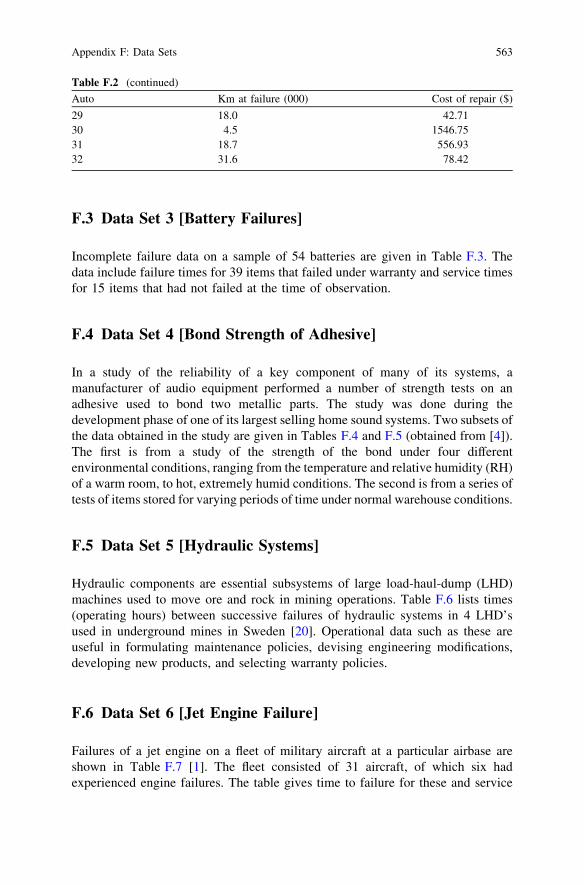
F.3 Data Set 3 [Battery Failures]

Incomplete failure data on a sample of 54 batteries are given in Table F.3. Thedata include failure times for 39 items that failed under warranty and service timesfor 15 items that had not failed at the time of observation.

F.4 Data Set 4 [Bond Strength of Adhesive]

In a study of the reliability of a key component of many of its systems, amanufacturer of audio equipment performed a number of strength tests on anadhesive used to bond two metallic parts. The study was done during thedevelopment phase of one of its largest selling home sound systems. Two subsets ofthe data obtained in the study are given in Tables F.4 and F.5 (obtained from [4]).The first is from a study of the strength of the bond under four differentenvironmental conditions, ranging from the temperature and relative humidity (RH)of a warm room, to hot, extremely humid conditions. The second is from a series oftests of items stored for varying periods of time under normal warehouse conditions.

F.5 Data Set 5 [Hydraulic Systems]

Hydraulic components are essential subsystems of large load-haul-dump (LHD)machines used to move ore and rock in mining operations. Table F.6 lists times(operating hours) between successive failures of hydraulic systems in 4 LHD’sused in underground mines in Sweden [20]. Operational data such as these areuseful in formulating maintenance policies, devising engineering modifications,developing new products, and selecting warranty policies.

F.6 Data Set 6 [Jet Engine Failure]

Failures of a jet engine on a fleet of military aircraft at a particular airbase areshown in Table F.7 [1]. The fleet consisted of 31 aircraft, of which six hadexperienced engine failures. The table gives time to failure for these and service

Table F.2 (continued)

Auto Km at failure (000) Cost of repair ($)

29 18.0 42.7130 4.5 1546.7531 18.7 556.9332 31.6 78.42

Appendix F: Data Sets 563

Table F.3 Battery failure data

Time to failure Service time

64 599 852 13166 619 929 162164 631 948 163178 639 973 202185 645 977 232299 656 1084 245319 681 1100 286383 722 1100 302385 727 1350 315405 738 337482 761 845492 765 983506 788 1259548 801 1384589 848 1421

Table F.4 Bond strength (pounds) under various test conditions

Test conditions

27�C, 50% RH 27�C, 70% RH 32�C, 70% RH 27�C, 100% RH

345 210 378 45230 272 254 426 210 278 1291 247 253 4222 223 359 3325 263 276 132251 9 245 8131 265 282 1322 214 308 48237 32 126 48 282 265306 1 24545 276 266272 202 289264 231 176277 251 273332 5 253100 75 3207 325 139254 50 266157 240260 68204 233


Table F.5 Bond strength (pounds) versus length of storage (days)Days Strength Days Strength Days Strength

3 296 11 278 52 2643 337 11 271 52 3063 266 11 316 52 2904 197 12 312 68 2124 312 12 308 68 2684 317 12 309 68 2905 309 13 289 75 3185 297 13 212 75 2605 296 13 249 75 2466 307 14 298 80 2906 298 14 252 80 2716 320 14 326 80 3607 323 17 332 82 2947 287 17 247 82 3567 344 17 311 82 28410 352 49 23710 235 49 27810 290 49 217

Table F.6 Time (hours) between failures of hydraulic systems in LHD’sLHD1 LHD3 LHD11 LHD17

327 637 353 401125 40 96 367 397 49 186 36 211 159107 54 82 341277 53 175 17154 97 79 24332 63 117 350510 216 26 72110 118 4 30310 125 5 349 25 60 4585 4 39 32427 101 35 259 184 258 7016 167 97 578 81 59 10334 46 3 1121 18 37 5152 32 8 3158 219 245 14444 405 79 8018 20 49 53

248 31 84140 259 218

283 122150

24


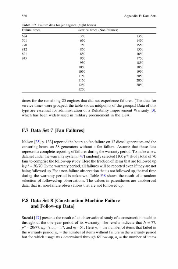
times for the remaining 25 engines that did not experience failures. (The data forservice times were grouped; the table shows midpoints of the groups.) Data of thistype are essential for administration of a Reliability Improvement Warranty [3],which has been widely used in military procurement in the USA.

F.7 Data Set 7 [Fan Failures]

Nelson [35, p. 133] reported the hours to fan failure on 12 diesel generators and thecensoring hours on 58 generators without a fan failure. Assume that these datarepresent a complete reporting of failures during the warranty period. To make a newdata set under the warranty system, [47] randomly selected (100 p*)% of a total of 70fans to comprise the follow-up study. Here the fraction of items that are followed upis p* = 30/70. In the warranty period, all failures will be reported even if they are notbeing followed up. For a non-failure observation that is not followed up, the real timeduring the warranty period is unknown. Table F.8 shows the result of a randomselection of followed-up observations. The values in parentheses are unobserveddata, that is, non-failure observations that are not followed up.

F.8 Data Set 8 [Construction Machine Failureand Follow-up Data]

Suzuki [47] presents the result of an observational study of a construction machinethroughout the one-year period of its warranty. The results indicate that N = 77,p* = 20/77, nu= 9, nc = 17, and nl = 51. Here nu = the number of items that failed inthe warranty period, nc = the number of items without failure in the warranty periodbut for which usage was determined through follow-up, nl = the number of items

Table F.7 Failure data for jet engines (flight hours)

Failure times Service times (Non-failures)

684 350 1350701 650 1450770 750 1550812 850 1550821 850 1650845 950 1750

950 18501050 18501050 19501150 20501150 20501250 20501250


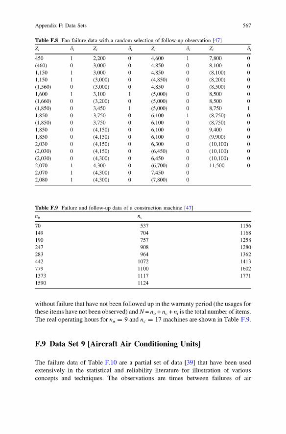
without failure that have not been followed up in the warranty period (the usages forthese items have not been observed) and N = nu + nc + nl is the total number of items.The real operating hours for nu = 9 and nc = 17 machines are shown in Table F.9.

F.9 Data Set 9 [Aircraft Air Conditioning Units]

The failure data of Table F.10 are a partial set of data [39] that have been usedextensively in the statistical and reliability literature for illustration of variousconcepts and techniques. The observations are times between failures of air

Table F.8 Fan failure data with a random selection of follow-up observation [47]

Zi di Zi di Zi di Zi di

450 1 2,200 0 4,600 1 7,800 0(460) 0 3,000 0 4,850 0 8,100 01,150 1 3,000 0 4,850 0 (8,100) 01,150 1 (3,000) 0 (4,850) 0 (8,200) 0(1,560) 0 (3,000) 0 4,850 0 (8,500) 01,600 1 3,100 1 (5,000) 0 8,500 0(1,660) 0 (3,200) 0 (5,000) 0 8,500 0(1,850) 0 3,450 1 (5,000) 0 8,750 11,850 0 3,750 0 6,100 1 (8,750) 0(1,850) 0 3,750 0 6,100 0 (8,750) 01,850 0 (4,150) 0 6,100 0 9,400 01,850 0 (4,150) 0 6,100 0 (9,900) 02,030 0 (4,150) 0 6,300 0 (10,100) 0(2,030) 0 (4,150) 0 (6,450) 0 (10,100) 0(2,030) 0 (4,300) 0 6,450 0 (10,100) 02,070 1 4,300 0 (6,700) 0 11,500 02,070 1 (4,300) 0 7,450 02,080 1 (4,300) 0 (7,800) 0

Table F.9 Failure and follow-up data of a construction machine [47]

nu nc

70 537 1156149 704 1168190 757 1258247 908 1280283 964 1362442 1072 1413779 1100 16021373 1117 17711590 1124


conditioning units on commercial aircraft. The original data set reported byProschan included data on thirteen aircraft. The results for three of these are givenin Table F.10.

F.10 Data Set 10 [Valve Seat for Diesel Engines]

Table F.11 shows engine age (in days) at the time of a valve seat replacement for afleet of 41 diesel engines. These data on a sample of systems appeared in [36, 37]and also in [30], p. 635.

Table F.10 Time between failures of AC units

Failure Aircraft

TBF-7909 TBF-7912 TBF-7913

1 90 23 972 10 261 513 60 87 114 186 7 45 61 120 1416 49 14 187 14 62 1428 24 47 689 56 225 7710 20 71 8011 79 246 112 84 21 1613 44 42 10614 59 20 20615 29 5 8216 118 12 5417 25 120 3118 156 11 21619 310 3 4620 76 14 11121 26 71 3922 44 11 6323 23 14 1824 62 11 19125 130 16 1826 208 90 16327 70 1 2428 101 1629 208 52


Table F.11 Diesel engine age at time of replacement of valve seats

System ID Days observed Engine age at replacement time

251 761252 759327 667 98328 667 326 653 653329 665330 667 84331 663 87389 653 646390 653 92391 651392 650 258 328 377 621393 648 61 539394 644 254 276 298 640395 642 76 538396 641 635397 649 349 404 561398 631399 596400 614 120 479401 582 323 449402 589 139 139403 593404 589 573405 606 165 408 604406 594 249407 613 344 497408 595 265 586409 389 166 206 348410 601411 601 410 581412 611413 608414 587415 603 367416 585 202 563 570417 587418 578419 578420 586421 585422 582


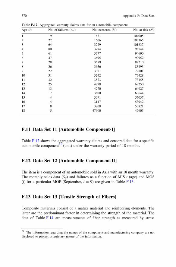
F.11 Data Set 11 [Automobile Component-I]

Table F.12 shows the aggregated warranty claims and censored data for a specificautomobile component21 (unit) under the warranty period of 18 months.

F.12 Data Set 12 [Automobile Component-II]

The item is a component of an automobile sold in Asia with an 18 month warranty.The monthly sales data (Sij) and failures as a function of MIS t (age) and MOS(j) for a particular MOP (September, i = 9) are given in Table F.13.

F.13 Data Set 13 [Tensile Strength of Fibers]

Composite materials consist of a matrix material and reinforcing elements. Thelatter are the predominant factor in determining the strength of the material. Thedata of Table F.14 are measurements of fiber strength as measured by stress

Table F.12 Aggregated warranty claims data for an automobile component

Age (t) No. of failures (n�t) No. censored (~nt) No. at risk (Nt)

1 9 631 1040052 22 1506 1033653 64 3229 1018374 80 3774 985445 61 3677 946906 47 3695 909527 28 3689 872108 36 3656 834939 22 3351 7980110 31 3242 7642811 32 3873 7315512 25 4298 6925013 13 4270 6492714 7 3600 6064415 4 3091 5703716 4 3117 5394217 8 3208 5082118 5 47600 47605


21 The information regarding the names of the component and manufacturing company are notdisclosed to protect proprietary nature of the information.

applied until fracture failure of silicon carbide fibers after extraction from aceramic matrix [49]. One of the objectives of the experiment was to comparestrengths of fibers of varying lengths. Fiber lengths used in the study were 5, 12.5,25.4, and 265 mm. Sample sizes of 50 were used for all but the 25.4 mm fibers, forwhich a sample of size 64 was used.

F.14 Data Set 14 [Automobile Component-III]

Table F.15 shows a part of the warranty claims data for an automobile component(20 observations out of 498).22 Failure modes, type of automobile used thecomponent and auto-used Zone/Region are shown in codes.

Table F.13 Monthly sales ðSijÞ and failures ðnitÞ indexed by MOS (j) and MIS (t) for a particularMOP (i = 9)

j Sij Failures {nit} in MIS (t) under warranty Tot

1 2 3 4 5 6 7 8 9 10 11 12 13 14 15 16 17 18

1 1064 1 1 2 1 1 2 1 1 1 1 122 3600 4 5 1 1 3 5 6 4 5 4 3 4 3 3 5 7 5 683 2113 1 1 2 3 2 1 1 2 5 2 3 2 1 3 294 720 1 1 1 1 1 1 1 1 1 1 1 115 442 1 3 2 1 1 86 235 1 2 1 1 1 1 77 168 08 94 09 74 1 2 310 90 1 1 211 51 1 1 212 16 013 63 014 82 1 1 2 415 51 016 27 017 8 018 20 019 12 020 8 1 1Tot 8938 6 8 3 5 6 7 9 12 8 10 10 13 8 8 9 6 9 10 147


22 The information regarding the names of the component and manufacturing company are notdisclosed to protect proprietary nature of the information.

F.15 Data Set 15 [Aircraft Windshield]

The windshield on a large aircraft is a complex piece of equipment, comprisedbasically of several layers of material, including a very strong outer skin with aheated layer just beneath it, all laminated under high temperature and pressure.Failures of these items are not structural failures. Instead, they typically involvedamage or delamination of the non-structural outer ply, or failure of the heatingsystem. These failures do not result in damage to the aircraft, but do result inreplacement of the windshield because of decreased visibility.

Table F.14 Tensile Strength of SiC Fibers

Fiber length (mm)

5 12.7 25.4 265 5 12.7 25.4 265

2.36 1.96 1.25 0.36 3.81 3.29 2.81 1.932.40 1.98 1.50 0.50 3.88 3.30 2.82 1.962.54 2.06 1.57 0.57 3.93 3.36 2.90 1.972.67 2.07 1.85 0.95 3.94 3.39 2.92 1.992.68 2.07 1.92 0.99 3.94 3.39 2.93 2.042.69 2.11 1.94 1.09 3.94 3.41 3.02 2.062.70 2.22 2.00 1.09 3.98 3.41 3.11 2.062.77 2.25 2.02 1.33 4.04 3.43 3.11 2.082.77 2.39 2.13 1.33 4.07 3.52 3.14 2.112.79 2.42 2.17 1.37 4.08 3.72 3.20 2.262.83 2.63 2.17 1.38 4.08 3.96 3.20 2.272.91 2.67 2.20 1.38 4.16 4.07 3.22 2.273.04 2.75 2.23 1.39 4.18 4.09 3.26 2.383.05 2.75 2.24 1.41 4.22 4.13 3.29 2.393.06 2.75 2.30 1.42 4.24 4.13 3.30 2.473.24 2.89 2.33 1.42 4.35 4.14 3.34 2.483.27 2.93 2.42 1.45 4.37 4.15 3.35 2.733.28 2.95 2.43 1.49 4.50 4.29 3.37 2.743.34 2.96 2.45 1.50 3.433.36 2.97 2.49 1.56 3.433.39 3.00 2.51 1.57 3.473.51 3.03 2.54 1.57 3.613.53 3.04 2.57 1.75 3.613.59 3.05 2.62 1.78 3.623.63 3.07 2.66 1.79 3.643.64 3.08 2.68 1.79 3.723.64 3.13 2.71 1.82 3.793.66 3.20 2.72 1.83 3.843.71 3.22 2.76 1.86 3.933.73 3.23 2.79 1.89 4.033.75 3.26 2.79 1.90 4.073.78 3.27 2.80 1.92 4.13


Tab

leF

.15

Det

aile

dw

arra

nty

clai

ms

data

ofan

auto

mob

ile

com

pone

nt

Ser

ial

no.

Dat

eof

prod

ucti

onD

ate

ofsa

leD

ate

offa

ilur

eA

gein

days

Use

dK

Mat

fail

ure

Fai

lure

mod

eU

sed

regi

onT

ype

ofau

tous

edth

eun

it

101

-Aug

-01

01-S

ep-0

115

-Jan

-02

136

3648

7M

2R

1A

22

01-M

ay-0

102

-Sep

-01

15-D

ec-0

110

423

81M

2R

4A

23

01-F

eb-0

107

-Sep

-01

15-D

ec-0

199

1450

7M

2R

3A

24

10-J

an-0

112

-Sep

-01

15-D

ec-0

194

7377

M1

R4

A2

501

-May

-01

12-S

ep-0

115

-Dec

-01

9410

790

M1

R4

A1

605

-Jul

-01

12-S

ep-0

115

-Feb

-02

156

4731

2M

3R

1A

17

05-A

pr-0

113

-Sep

-01

05-J

ul-0

229

556

943

M2

R4

A1

810

-Jun

-01

15-S

ep-0

112

-Jul

-02

300

4529

2M

1R

3A

29

05-A

pr-0

122

-Sep

-01

15-N

ov-0

154

5187

M2

R3

A1

1001

-Aug

-00

24-S

ep-0

115

-Dec

-01

8245

12M

3R

1A

111

01-D

ec-0

027

-Sep

-01

15-M

ar-0

216

918

175

M1

R3

A1

1210

-Jan

-01

27-S

ep-0

115

-Mar

-02

169

1810

6M

1R

3A

113

01-A

pr-0

127

-Sep

-01

26-S

ep-0

236

427

008

M1

R3

A2

1405

-Apr

-01

28-S

ep-0

115

-Dec

-01

7811

600

M1

R4

A1

1501

-May

-01

28-S

ep-0

115

-Dec

-01

7879

00M

1R

4A

116

10-J

un-0

129

-Sep

-01

15-D

ec-0

177

1762

0M

1R

4A

117

10-J

un-0

129

-Sep

-01

15-O

ct-0

116

7762

M1

R4

A1

1810

-Jun

-01

01-O

ct-0

115

-Mar

-02

165

3948

7M

1R

3A

119

01-J

un-0

002

-Oct

-01

15-N

ov-0

144

6420

M1

R3

A2

2001

-Mar

-01

07-O

ct-0

110

-Apr

-02

185

4512

1M

2R

4A

1


Table F.16 Windshield failure and censored data

Failure times (thousand hours) Service times (thousand hours)

0.040 1.866 2.385 3.443 0.046 1.436 2.5920.301 1.876 2.481 3.467 0.140 1.492 2.6000.309 1.899 2.610 3.478 0.150 1.580 2.6700.557 1.911 2.625 3.578 0.248 1.719 2.7170.943 1.912 2.632 3.595 0.280 1.794 2.8191.070 1.914 2.646 3.699 0.313 1.915 2.8201.124 1.981 2.661 3.779 0.389 1.920 2.8781.248 2.010 2.688 3.924 0.487 1.963 2.9501.281 2.038 2.823 4.035 0.622 1.978 3.0031.281 2.085 2.890 4.121 0.900 2.053 3.1021.303 2.089 2.902 4.167 0.952 2.065 3.3041.432 2.097 2.934 4.240 0.996 2.117 3.4831.480 2.135 2.962 4.255 1.003 2.137 3.5001.505 2.154 2.964 4.278 1.010 2.141 3.6221.506 2.190 3.000 4.305 1.085 2.163 3.6651.568 2.194 3.103 4.376 1.092 2.183 3.6951.615 2.223 3.114 4.449 1.152 2.240 4.0151.619 2.224 3.117 4.485 1.183 2.341 4.6281.652 2.229 3.166 4.570 1.244 2.435 4.8061.652 2.300 3.344 4.602 1.249 2.464 4.8811.757 2.324 3.376 4.663 1.262 2.543 5.1401.795 2.349 3.385 4.694 1.360 2.560 –

Table F.17 Photocopier’s service history data

Counter Day Component Counter Day Component

60152 29 Cleaning Web 365075 397 Toner Filter60152 29 Toner Filter 365075 397 Drum Claws60152 29 Feed Rollers 365075 397 Ozone Filter132079 128 Cleaning Web 370070 468 Feed Rollers132079 128 Drum Cleaning Blade 378223 492 Drum132079 128 Toner Guide 390459 516 Upper Fuser Roller220832 227 Toner Filter 427056 563 Cleaning Web220832 227 Cleaning Blade 427056 563 Upper Fuser Roller220832 227 Dust Filter 449928 609 Toner Filter220832 227 Drum Claws 449928 609 Feed Rollers252491 276 Drum Cleaning Blade 449928 609 Upper Roller Claws252491 276 Cleaning Blade 472320 677 Feed Rollers252491 276 Drum 472320 677 Cleaning Blade252491 276 Toner Guide 472320 677 Upper Roller Claws365075 397 Cleaning Web 501550 722 Cleaning Web501550 722 Dust Filter 933637 1410 Feed Rollers501550 722 Drum 933637 1410 Dust Filter501550 722 Toner Guide 933637 1410 Ozone Filter533634 810 TS Block Front 933785 1412 Cleaning Web

(continued)


Data on failure and service times for a particular model windshield are given inTable F.16 (from [4]). The data consist of 153 observations, of which 88 areclassified as failed windshields and the remaining 65 are service times ofwindshields that had not failed at the time of observation.

F.16 Data Set 16 [Photocopier]

The data recorded from the photocopier’s service history are given in Table F.17.Each row describes a part that was replaced, giving the number of copies made atthe time of replacement, the age of the machine in days, and the componentreplaced. Most services involved replacing multiple components.

Table F.17 (continued)

Counter Day Component Counter Day Component

533634 810 Charging Wire 936597 1436 Drive Gear D583981 853 Cleaning Blade 938100 1448 Cleaning Web597739 916 Cleaning Web 944235 1460 Dust Filter597739 916 Drum Claws 944235 1460 Ozone Filter597739 916 Drum 984244 1493 Feed Rollers597739 916 Toner Guide 984244 1493 Charging Wire624578 956 Charging Wire 994597 1514 Cleaning Web660958 996 Lower Roller 994597 1514 Ozone Filter675841 1016 Cleaning Web 994597 1514 Optics PS Felt675841 1016 Feed Rollers 1005842 1551 Upper Fuser Roller684186 1074 Toner Filter 1005842 1551 Upper Roller Claws684186 1074 Ozone Filter 1005842 1551 Lower Roller716636 1111 Cleaning Web 1014550 1560 Feed Rollers716636 1111 Dust Filter 1014550 1560 Drive Gear D716636 1111 Upper Roller Claws 1045893 1583 Cleaning Web769384 1165 Feed Rollers 1045893 1583 Toner Guide769384 1165 Upper Fuser Roller 1057844 1597 Cleaning Blade769384 1165 Optics PS Felt 1057844 1597 Drum787106 1217 Cleaning Blade 1057844 1597 Charging Wire787106 1217 Drum Claws 1068124 1609 Cleaning Web787106 1217 Toner Guide 1068124 1609 Toner Filter840494 1266 Feed Rollers 1068124 1609 Ozone Filter840494 1266 Ozone Filter 1072760 1625 Feed Rollers851657 1281 Cleaning Blade 1072760 1625 Dust Filter851657 1281 Toner Guide 1072760 1625 Ozone Filter872523 1312 Drum Claws 1077537 1640 Cleaning Web872523 1312 Drum 1077537 1640 Optics PS Felt900362 1356 Cleaning Web 1077537 1640 Charging Wire900362 1356 Upper Fuser Roller 1099369 1650 TS Block Front900362 1356 Upper Roller Claws 1099369 1650 Charging Wire



References

1. Abernethy RB, Breneman JR, Medlin CH, Reinman GL (1983) Weibull analysis handbook.Report No. AFWAL-TR-83-2079, Aero Propulsion Laboratory, USAF, Wright-PattersonAFB, Ohio

2. Abramowitz M, Stegun IA (1964) Handbook of mathematical functions. AppliedMathematics Series No. 55, National Bureau of Standards, Washington, D.C.

3. Blischke WR, Murthy DNP (1994) Warranty cost analysis. Dekker, New York4. Blischke WR, Murthy DNP (2000) Reliability. Wiley, New York5. Casella G, Berger RL (2001) Statistical inference. Duxbury, New York6. Cox DR, Isham V (1980) Point processes. Chapman and Hall, London7. Dempster AP, Laird NM, Rubin DB (1977) Maximum likelihood from incomplete data via

the EM algorithm (with discussion). J Royal Statist Soc B 39:1–388. Dodson B (1994) Weibull analysis. ASQ Quality Press, Milwaukee, Wisconsin9. Gumbel EJ (1960) Bivariate exponential distributions. J Am Statist Assoc 55:698–707

10. Hartley HQ (1958) Maximum likelihood estimation from incomplete data. Biometrics14:174–194

11. Hogg RV, Craig A, McKean JW (2004) Introduction to mathematical statistics, 6th edn.Prentice Hall, New York

12. Hutchinson TP, Lai CD (1990) Continuous bivariate distributions-emphasising applications.Rumsby Scientific, Adelaide, Australia

13. Hunter JJ (1974) Renewal theory in two dimensions: basic results. Adv App Probab6:376–391

14. Johnson NL, Kotz S (1969) Discrete distributions. Houghton Mifflin Co., Boston15. Johnson NL, Kotz S (1969) Distributions in statistics: discrete distributions. Wiley,

New York16. Johnson NL, Kotz S (1970) Distributions in statistics: continuous univariate distributions-I.

Wiley, New York17. Johnson NL, Kotz S (1970) Distributions in statistics: continuous univariate distributions-II.

Wiley, New York18. Johnson NL, Kotz S (1972) Distributions in statistics: continuous multivairate distributions.

Wiley, New York19. Kies JA (1958) The strength of glass, Naval Res-Lab. Report No. 5093, Washington D.C.20. Kumar U, Klefsjö B (1992) Reliability analysis of hydraulic systems of LHD machines using

the power law process model. Reliab Eng Sys Saf 35:217–22421. Lai CD, Xie M, Murthy DNP (2003) Modified Weibull model. IEEE Tran Rel 52:33–3722. Lawless JF (1982) Statistical methods for lifetime data. Wiley, New York23. Lee L (1979) Multivariate distributions having Weibull properties. J Multivar Analysis

9:267–27724. Lehman EL, Casella G (1998) Theory of point estimation. Springer, New York25. Little RJA, Rubin DB (1987) Statistical analysis with missing data. Wiley, New York26. Louis TA (1982) Finding the observed information matrix when using the EM algorithm.

J Royal Statist Soc B 44:226–23327. Lu JC, Bhattacharyya GK (1990) Some new constructions of bivariate Weibull Models. Ann

Inst Statist Math 42:543–55928. McLachlan GJ, Krishnan T (1997) The EM algorithm and extensions. Wiley, New York29. Marshall AW, Olkin I (1967) A multivariate exponential distribution. J Am Statist Assoc

62:30–4430. Meeker WQ, Escobar LA (1998) Statistical methods for reliability data. Wiley, New York31. Meng XL, Rubin DB (1991) Using EM to obtain asymptotic variance-covariance matrices:

the SEM algorithm. J Am Statist Assoc 86:899–909

32. Mudholkar GS, Kollia GD (1994) Generalized Weibull family: A structural analysis. Commin Stat Ser A: Theory and Methods 23:1149–1171

33. Murthy DNP, Bulmer M, Eccleston JE (2004) Weibull model selection. Reliab Eng Sys Saf86:257–267

34. Murthy DNP, Xie M, Jiang R (2003) Weibull models. Wiley, New York35. Nelson W (1982) Applied life data analysis. Wiley, New York36. Nelson W (1995) Confidence limits for recurrence data-applied to cost or number of product

repairs. Technometrics 37:147–15737. Nelson W, Doganaksoy N (1989) A Computer program for an estimate and confidence limits

for the mean cumulative function for cost or number of repairs of repairable products. TISreport 89CRD239, General Electric Company Research and Development, Schenectady, NY

38. Oakes D (1999) Direct calculation of the information matrix via the EM algorithm. J RoyalStatist Soc B 61:479–482

39. Proschan F (1963) Theoretical explanation of observed decreasing failure rate.Technometrics 5:375–383

40. Rao CR (1972) Linear statistical inference and its applications. Wiley, New York41. Redner RA, Walker HF (1984) Mixture densities, maximum likelihood and the EM

algorithm. SIAM Rev 26:195–23942. Rigdon SE, Basu AP (2000) Statistical methods for the reliability of repairable systems.

Wiley, New York43. Ross SM (1970) Applied probability models with optimization applications. Holden–Day

San, Francisco44. Ross SM (1980) Stochastic processes. Wiley, New York45. Somerville PN (1958) Tables for obtaining non-parametric tolerance limits. Ann Math Stat

29:599–60146. Stuart A, Ord JK (1991) Kendall’s advanced theory of statistics, vol 2, 5th edn. Oxford

University Press, New York47. Suzuki K (1985) Estimation of lifetime parameters from incomplete field data.

Technometrics 27:263–27148. Wu CFJ (1983) On the convergence properties of the EM algorithm. Ann Statist 11:95–10349. Zok FW, Chen X, Weber DH (1995) Tensile strength of SiC fibers. J Am Ceram Soc

78:1965–1968


Index

AAcceleration factor, 323AD statistic, 187AD* statistics, 200Additional data

historical, 421market related, 420technology related, 420

AFT model, 119, 322, 335Arrhenius, 323Eyring, 323inverse power, 323likelihood function, 336linear, 323

Agency theory, 402Aggregated claims, 352Aggregation, 392Agreement

contractual, 400Air conditioner, 439Akaike information criterion

AIC, 293Analysis

cause-and-effect, 385levels, 163, 392parametric, 191qualitative, 11quantitative, 11

Analysis of variance, 242test of assumptions, 123

Anderson-Darling testparameters estimated, 236

ANOVA, 241assumptions, 455

Assembly error, 46

Assembly errors, 46Assumption

distributional, 259validity, 258

Attribution theory, 395Autocorrelation, 259Automobile, 4Automobile component, 476Average, 166

BBartlett’s test, 260, 456Bayes Theorem, 208Bayesian

analysis, 257inference, 385

Bill of materials, 407Block diagram, 256Blocks, 245Boxplot, 230, 448Brainstorming, 385Buyer

corporation, 20government agency, 20individual 20

CCause-effect, 43CDF

nonparametric estimation, 269Cell phone, 2Censoring

extreme, 464Type I, 83Type II, 83


579

C (cont.)Chart

MOP-TTF, 452Chi-square

goodness-of-fit test, 229Chi-square distribution

table, 549Claim

automatic processing, 412Claims data

classification, 67problems, 70

Claims ratecumulative, 311

Classificationone-way, 241two-way, 241, 246

Clockage, 97calendar, 97

Coefficientcorrelation, 169, 479of variation, 168, 365, 497rank correlation, 169

Comparing meansnormal distribution, 241two exponential distributions, 222two normal distributions, 221

Comparison procedureTukey’s multiple, 456, 483

Competing risk model, 320, 328cumulative hazard function, 321hazard function, 321likelihood function, 329reliability function, 321

Complainthandling, 398

Componentcause of failure, 393conformance, 32non-conformance, 40, 48reliability, 35, 54specification, 408

Composite scale, 145, 354, 497Conditional expectation, 520Confidence interval, 193, 211

binomial distribution, 213exponential distribution, 223gamma distribution, 214lognormal distribution, 214normal approximation, 279normal distribution, 212one-sided, 212Poisson distribution, 213

system reliability, 256two-sided, 211Weibull distribution, 214

Consumeraffairs, 20dissatisfaction, 395durables, 3expectation, 6movements, 20needs, 6non-durables, 3satisfaction, 395

Continuous distribution fitting, 235Continuous improvement, 10, 381

process, 289, 412Contract, 39, 426

incentive, 402Contracts, 33Copula, 148Correlation

rank, 169Correlation coefficients, 483Cost

estimation, 428sharing, 28

Counting process, 52, 297Courts, 20Covariance, 169Covariates, 319Cox PH model, 323Cramér-Rao inequality, 539Critical incidents, 388Cumulative

failure rate function, 45hazard function, 45intensity function, 297

Cumulative damage, 38Cumulative hazard function

estimate, 271Cumulative process, 527Customer

assurance, 1behavior, 1complaints, 389dissatisfaction, 6, 31needs, 407requirements, 38satisfaction, 28, 427surveys, 387

DData, 61, 159

censored, 12, 80, 81, 176, 480claims, 10, 477

580 Index

classification, 85coding, 163complete, 196cost related, 67customer related, 10, 67Design phase, 86Development phase, 87failure, 162Feasibility phase, 86field, 9grouped, 163, 205improper collection, 12incomplete, 196, 201left censored, 83life cycle, 83market related, 10Marketing phase, 88messy, 230mining, 75, 161multiply censored, 83, 276post warranty, 89post-production, 80, 88pre-production, 80, 86problems, 10, 161product related, 10, 67production, 80qualitative, 173retailer, 86right censored, 83scenarios, 103service agent related, 10, 67singly censored, 83Structure 1, 96Structure 2, 96Structure 3, 97structured, 62structures, 96supplementary, 10, 93, 479text, 161transformation, 259unstructured, 62

Data analysisnonparametric approach, 354, 356parametric approach, 373preliminary, 159

Data collectioninterval, 101

Data set, 561large, 160, 186

Database, 479Deductibles, 28Defect code, 389Density function, 513

conditional, 519joint, 519

Designblock randomized complete, 245completely randomized, 241outsourcing, 392problems, 407randomized complete block, 241reliability, 40specifications, 48

Design of Experiments (DOE), 241Diffusion model, 120Discrete distribution fitting, 234Distribution

Bernoulli, 511binomial, 197, 257, 511bivariate exponential, 521bivariate normal, 520bivariate Weibull, 521competing risk, 515derived, 515exponential, 197, 513exponentiated Weibull, 517extended Weibull, 516F, 518fitting, 460four parameter Weibull, 517Frechet, 515gamma, 198, 513gaussian (normal), 513geometric, 512hypergeometric, 197, 512inverse gaussian, 199, 516largest extreme value, 515loglogistic, 303lognormal, 199, 466, 516modified Weibull, 516multinomial, 512multiplicative, 517normal, 168, 199of mixtures, 517Poisson, 197, 512smallest extreme value, 514student-t, 518three-parameter Weibull, 516uniform (rectangular), 514Weibull, 198, 337, 514

Distribution function, 509bivariate, 354conditional, 519empirical, 175joint, 519marginal, 519

Index 581

D (cont.)Distribution-free

methods, 267Distributions

bivariate, 145Distributor, 20Drill-down process, 393

EEarly warning system, 413EDF, 461EM algorithm, 545Engineering

analysis, 27judgment, 1

Error, 36Type 1, 389Type 2, 389Type I, 217Type II, 217types, 389

Estimate, 193cumulative hazard function, 272distribution function, 278point, 538

EstimationBAN, 538Bayes, 208, 538confidence interval, 211, 538cost model, 251function of parameters, 250hazard function, 278intensity function, 257least squares, 538maximum likelihood, 196MCF, 272method of least squares, 208method of moments, 206minimum chi-square, 538moment, 538reliability, 278theory, 537

Estimator, 193asymptotic properties, 195asymptotic unbiasedness, 539best, 195consistency, 195, 539efficiency, 195, 539hazard function, 276Kaplan-Meier, 176, 272maximum likelihood, 196, 540point, 538product limit, 272

properties, 194standard error, 211sufficiency, 195, 539unbiasedness, 195, 539

Euler constant, 515Exclusion, 28Expectation

partial, 252Exponential distribution

estimation of reliability, 253External parties, 32

FF distribution

table, 550Failure

catastrophic, 37complete, 37degraded, 37density function, 44distribution function, 45extended, 37gradual, 37intermittent, 37mechanism, 37not reported, 72partial, 37rate function, 45sudden, 37

Failure cause, 37aging, 37design, 37manufacturing, 37mishandling, 37misuse, 37weakness, 37

Failure mechanismoverstress, 38wear-out, 38

Failure mode, 37, 327, 481Failure rate

baseline, 323constant, 46decreasing, 46increasing, 46

Failuresover time, 52

Fault, 36Fault tree, 54Fault tree analysis, 54, 385Federal Transport Authority (FTA), 404Fisher information, 540Fitting

582 Index

continuous distribution, 235discrete distributions, 234

Fleming-Harringtonestimate, 277

Forecastingwarranty claims, 375, 504warranty costs, 375

Fractile, 165, 511Fraud, 398Fraudulent claim, 65Function

gamma, 514

GGK approach, 364GLM, 490Goodness-of-fit test

in model building, 239incomplete data, 239

Graphical methods, 183, 209Grubb’s test, 232, 449Guarantee, 7

HHazard function, 45

estimator, 276Histogram, 171, 446Hypothesis

alternate, 216composite, 216null, 216

Hypothesis testing, 216

IImperfect repair model, 345

likelihood function, 346Implied warranty

of fitness, 21of merchantability, 21

Industry practice, 94Inferential statistics, 191Information, 62

loss, 73Inspection, 159Intensity function, 53, 297, 524

estimation, 257log linear, 298power law process, 298

Ishikawa diagram, 385

JJustice

distributive, 398

interactional, 398procedural, 398

KKaplan-Meier

estimate, 277estimator, 272method, 275

Key performance indicators, 413Knowledge, 62Kolmogorov-Smirnov test, 235Kolomogorov-Smirnov test

parameter estimated, 236Kruskal-Wallis Test, 458

LLeast squares, 239

fit, 239method, 247

Levene’s test, 260, 456Life cycle

cost, 132, 428Life cycle cost

customer, 115manufacturer, 115

Life-stress relationship, 336Likelihood function, 196, 540

Cox’s partial, 342Linear regression

inference, 247Logic tree diagram, 385

MManagerial implications, 491Manufacturing process, 39Marketing, 428Maximum likelihood, 196MCF

estimation, 272Mean cumulative function (MCF), 526Measure of

center, 166dispersion, 167location, 166

Measurementscales, 162

Median, 511Military handbook test, 300Mixture model, 332

density function, 322hazard function, 322likelihood function, 333reliability function, 322

Index 583

M (cont.)ML estimator

exponential distribution, 202properties, 205Weibull distribution, 203

Modelaccelerated failure time (AFT), 50, 319analysis, 44building, 42competing risk, 48, 320imperfect repair, 321linear, 242mathematical, 42mixture, 48, 320physical, 42probability, 238proportional hazards, 50, 319selection, 44, 183, 238, 292, 533semi-parametric, 324stress-strength, 257validation, 44, 185, 292

Modelingdata-dependent, 292empirical, 44physics-based, 44, 292process, 43

Models, 11, 42Moment

central, 511first, 510second, 511

Moment estimator, 207Month in service, 281Month of production, 281MOP-MIS, 278

diagram, 281, 502Multiple customers, 298

NNew product development, 415NHPP

likelihood function, 308No fault found, 389Nonparametric, 191

approach, 268confidence interval, 268methods, 267tolerance interval, 268

Nonparametric estimationCDF, 269renewal function, 269, 270

Nonparametric estimatorrenewal function, 270

Nonparametric methods, 224Freidman test, 227Kruskal-Wallis test, 227Mann-Whitney test, 226rank sum test, 226signed rank test, 225

Nonparametric tolerance intervalsfactors for calculating, 558

Non-stationary Poisson process, 53Normal distribution

factors for tolerance intervals, 554table, 547

NPDLevel I (business level), 423Level II (product level), 423Level III (component level), 423process, 422Stage I (pre-development), 423Stage II (development), 423Stage III (post-development), 423

OObservation, 164Operating environment, 50Operational data storage, 413Outlier, 166, 445, 448

dealing with, 232detection, 231

Out-source, 28Outsourcing, 425

design, 425production, 425servicing, 425

PParameter

estimate, 537estimation, 44, 193estimator, 537

Parametric modeladvantages, 293

Pareto chart, 170, 450, 481Partial expectation, 314PDCA cycle, 382Percentile, 164Performance, 5

field, 10measures, 381

PH model, 119, 323, 341likelihood function, 341

Pie chart, 173Plot

EDF, 529

584 Index

empirical, 529exponential probability, 533extreme large value probability, 534extreme small value probability, 534Frechet probability, 535interaction, 486lognormal probability, 534main effect, 490normal distribution, 533residual, 261scatter, 479theoretical, 529time series, 389Weibull probability, 531whisker, 230WPP, 529

Point process, 523alternating renewal, 526compound Poisson, 527counting, 523cumulative intensity function, 524delayed renewal, 525intensity function, 524marked, 527one-dimensional, 523ordinary renewal, 524stationary Poisson, 524two-dimensional, 524two-dimensional renewal, 524

Post-sale, 8factors, 8support, 9

P-P plot, 177Prediction, 312

warranty claims, 312warranty costs, 312

Preprocessing, 161Probability

model, 238plot, 177, 181theory, 42, 509

Problemcustomer related, 390, 397design related, 391production related, 390service agent related, 400service related, 390

Problem solving, 383Product

architecture, 407attributes, 6, 420characteristics, 420classification, 3

commercial, 3complexity, 4, 415custom-built, 4decomposition, 4design, 1, 38deterioration, 36development, 1, 10, 20, 22, 39, 428failure, 6, 35industrial, 3launch, 35liability laws, 20life cycle, 2, 31, 35, 38, 40, 83, 115lifetime, 30management, 31misuse, 397non-repairable, 52obsolescence, 39performance, 5, 32, 36reliability, 9, 35, 39, 54repairable, 53requirement, 39sales, 31specialized, 3standard, 4, 38tangible, 2usage environment, 31usage intensity, 31variety, 429warranty, 7

Production, 1outsourcing, 425

Production data, 87Product-limit estimator, 272Public policy, 20Purchase

first, 31, 120repeat, 31, 121

P-value, 243

QQuality

of service, 396perceived, 396value-based, 396

Quality variationnon-conformance, 46

Quality variationsassembly error, 46

Quartile, 165, 511

RRandom variable, 509

moment, 510

Index 585

R (cont.)Random variables

independent, 519product, 544ratio, 544sum, 543

Rangeinterquartile, 168

Rank correlation, 227Rank sum test, 226Reasoning

deductive, 384inductive, 384

Recurrence rate, 526Regression

analysis, 246coefficient, 247multiple linear, 247prediction, 248test of assumptions, 261

Regression model, 320likelihood function, 343location-scale, 325parametric, 325, 342Weibull, 343

Reliabilityactual, 9assessment, 9, 92, 252at sale, 41block diagram, 54decision, 2design, 40field, 35, 41, 51, 467function, 40, 45inherent, 41linking, 54performance, 381predicted, 9specification, 40theory, 35

Reliability assessmentdata-based, 252

Renewalfunction, 525integral equation, 525process, 524

Renewal functionnonparametric estimation, 269nonparametric estimator, 270

Repair, 117imperfect, 53, 326minimal, 53rate, 118

Replace, 117Replicates, 245Reporting delays, 71Reputation, 427Residuals, 259

Cox-Snell, 339standardized, 339, 344

Response, 246Retailer, 20ROCOF, 297Root cause analysis, 385Run chart, 385

SSample, 164

CDF, 174correlation coefficient, 248mean, 166median, 166regression line, 248standard deviation, 167variance, 167

Scaleinterval, 162nominal, 162ordinal, 162ratio, 162

Serviceagent, 426contract, 7, 27cost, 118maintenance contract, 23time, 118

Service costdirect expense, 70indirect expenses, 70

Servicingoutsourcing, 425

Servicing strategy, 117SERVQUAL, 396Sign test, 225Signed rank test, 225Skewness, 167Spare part

management, 413Standard deviation, 511Statistic, 164Statistical inference, 164, 191Statistics, 42

descriptive, 166, 446, 478F, 243theoretical, 537

Strategic management

586 Index

business objectives, 418new product goals, 418

Strength, 38Stress, 38Student-t distribution

table, 548System

characterization, 43complexity, 5happy, 299parallel, 256sad, 299series, 256state, 54

TTarget levels, 381Targets

commercial, 428technical, 428

TestAnderson-Darling, 236Bartlett’s, 260, 456F, 243goodness-of-fit, 233Grubb’s, 449homogeneity of variance, 260independence, 258Kolmogorov-Smirnov, 235Kruskal-Wallis, 458Laplace, 300Levene’s, 260, 456military handbook, 300multiple comparison, 244one-tailed, 217randomness, 259runs, 259Tukey, 244two-tailed, 217

Testing hypothesisbinomial distribution, 219exponential distribution, 220lognormal distribution, 220normal distribution, 218Weibull distribution, 220

Thinkingconvergent, 385creative, 384divergent, 384innovative, 384lateral, 384

Toleranceinterval, 222

limit, 222Tolerance interval

nonparametric, 223normal, 223

Tolerance limitexponential distribution, 223

Total qualitymanagement (TQM), 381

Traceability, 93, 393part, 413

TREAD legislation, 404Treatment, 242

effect, 242groups, 242

Trimmed mean, 167Tukey test, 244Turnbull

estimate, 275survival plot, 275

Two-dimensional dataaggregated, 351alternate scenarios, 353alternate structures, 353detailed, 350nonparametric approach, 368parametric approach, 368supplementary, 352

UUniform commercial code, 21Usage, 138

different notions, 51intensity, 1, 50mode, 1

Usage data, 89Usage function

linear, 363Usage mode

intermittent, 49Usage rate, 355, 491

average, 356, 361median, 356

VVariability

sources, 243Variable

dependent, 246explanatory, 246predictor, 246

Variance, 511Variation

coefficient, 250

Index 587

V (cont.)extra-Poisson, 310

v-scale, 367

WWarranty, 1

accounting, 20administration, 20, 31base, 1behavioral, 20breadth, 417claim process, 64claims, 2, 121claims data, 10, 33, 67claims rate, 285, 309, 391classification, 22combination, 23consumerist, 20cost, 1, 8, 29cost analysis, 427cumulative, 26dashboard, 413data, 2, 10, 33, 35decision-making, 416economic, 20engineering, 20execution, 64execution function, 119exploitative theory, 416express, 21extended, 1, 7, 27flexible, 33, 426free replacement, 24historical, 20historical perspective, 415implied, 21legal, 20legislation, 8legislative, 20length, 417logistics, 402management, 20, 31, 381management system, 412, 431non-renewing, 23one-dimensional, 23, 80operations research, 20parameters, 23period, 23, 114, 141policies, 470policy, 10process, 63pro-rata, 24region, 26

renewing, 23servicing, 28, 33, 103servicing process, 65signaling theory, 416simple, 23societal, 20statistics, 20strategic management, 32supplementary data, 10, 33two-dimensional, 23, 25, 81, 137type, 417

Warranty ActsMagnuson-Moss Act, 21TREAD Act, 21

Warranty claims datatwo-dimensional, 349

Warranty costlife cycle, 29models, 116, 124per unit, 114prediction, 314repair limit, 117unit sale, 29

Warranty dataanalysis, 10problems, 2

Warranty managementfirst epoch, 416second epoch, 416Stage 1, 73, 90Stage 2, 74, 92Stage 3, 92third epoch, 418

Warranty policy2-D FRW, 262-D PRW, 26FRW, 439group FRW, 27non-renewing FRW, 24non-renewing PRW, 24reliability improvement, 27renewing FRW, 24renewing PRW, 24

Warranty servicingoperational, 28repair/replace, 28spare parts, 28strategic, 28

Warranty strategydefensive, 417offensive, 417

Weibullcompeting risk model, 461

588 Index

transform, 531Weibull distribution

estimation of reliability, 254

mixture, 461Wisdom, 62WPP plot, 179

Index 589

appendix a: basic concepts from probability theory978-0-85729-647-4/1.pdf · appendix a: basic...

Documents