appendix a: vector spaces - home - springer978-0-387-21544-0/1.pdf · the gmm-schmidt theorem. ......
TRANSCRIPT

Appendix A: Vector Spaces
This appendix reviews some of the basic definitions and properties of vector spaces. It is presumed that, with the possible exception of Theorem A.14, all of the material presented here is familiar to the reader.
Definition A.!. A set Me Rn is a vector space if, for any x, y, z E M and scalars a, f3, operations of vector addition and scalar multiplication are defined such that
(1) (x + y) + z = x + (y + z).
(2) x + y = y + x.
(3) There exists a vector 0 E M such that x + 0 = x = 0 + x for any xEM.
(4) For any x E M, there exists y == -x such that x + y = 0 = y + x.
(5) a(x+y) = ax + ay.
(6) (a + f3)x = ax + f3x.
(7) (af3)x = a(f3x).
(8) There exists a scalar e such that ex = x. (Typically, e = 1.)
Definition A.2. Let M be a vector space, and let N be a set with N eM. N is a subspace of M if and only if N is a vector space.

392 Appendix A: Vector Spaces
Vectors in Rn will be considered as n x 1 matrices. The 0 vector referred to in Definition A.I is just an n x 1 matrix of zeros. Think of vectors in three dimensions as (x, y, z)" where w' denotes the transpose of a matrix w. The subspace consisting of the z axis is
The subspace consisting of the x, y plane is
The subspace consisting of the plane that is perpendicular to the line x = y in the x, y plane is
Theorem A.3. Let M be a vector space, and let N be a nonempty subset of M. If N is closed under vector addition and scalar multiplication, then N is a subspace of M.
Theorem A.4. Let M be a vector space, and let Xl, ... ,Xr be in M. The set of all linear combinations of Xl, ... ,Xr is a subspace of M.
Definition A.5. The set of all linear combinations of Xl, . .. ,Xr is called the space spanned by Xl, •. ' ,Xr . If N is a subspace of M, and N equals the space spanned by Xl," . ,Xr, then {Xl, ... , x r } is called a spanning set for N.
For example, the space spanned by the vectors
consists of all vectors of the form (a, b, b)', where a and b are any real numbers.
Let A be an n x p matrix. Each column of A is a vector in Rn. The space spanned by the columns of A is called the column space of A and written C(A). (Some people refer to C(A) as the range space of A and write it
Appendix A: Vector Spaces 393
R{A).) If B is an n x r matrix, then C{A, B) is the space spanned by the p + r columns of A and B.
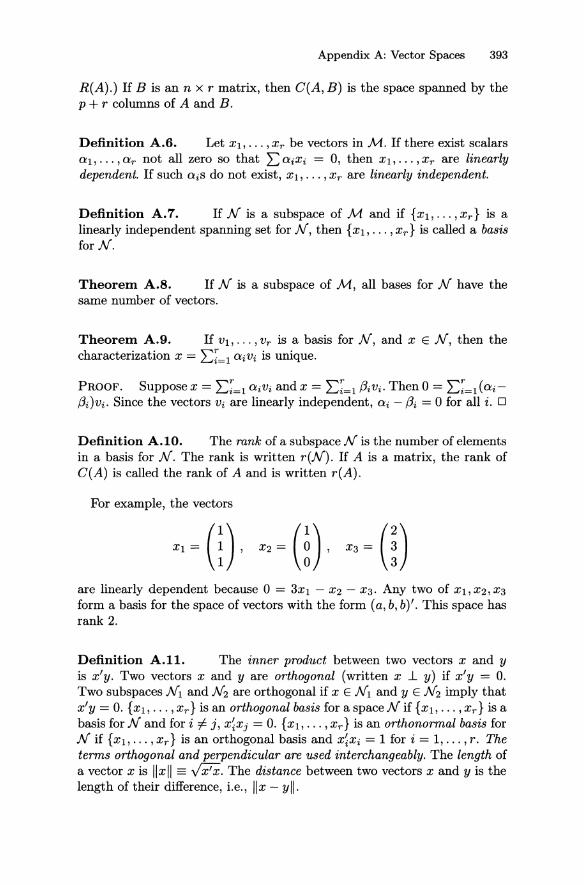
Definition A.6. Let Xl. ... ,Xr be vectors in M. If there exist scalars 01, ... ,Or not all zero so that L: 0iXi = 0, then Xl, ... , Xr are linearly dependent. If such 0iS do not exist, Xl, ... ,Xr are linearly independent.
Definition A. 7. If N is a subspace of M and if {Xl. .•. , xr } is a linearly independent spanning set for N, then {Xl, ... , X r } is called a basis forN.
Theorem A.S. If N is a subspace of M, all bases for N have the same number of vectors.
Theorem A.9. If VI. ... ,Vr is a basis for N, and X E N, then the characterization X = L:;=l 0iVi is unique.
PROOF. Suppose X = L:;=l 0iVi and X = L:;=l {3iVi. Then 0 = L:;=l {Oi{3i)Vi. Since the vectors Vi are linearly independent, 0i - {3i = 0 for all i. 0
Definition A.IO. The rank of a subspace N is the number of elements in a basis for N. The rank is written r{N). If A is a matrix, the rank of C(A) is called the rank of A and is written r(A).
For example, the vectors
are linearly dependent because 0 = 3Xl - X2 - X3. Any two of Xl,X2,X3
form a basis for the space of vectors with the form (a, b, b)'. This space has rank 2.
Definition A.II. The inner product between two vectors X and y is x'y. Two vectors X and y are orthogonal (written X 1- y) if x'y = o. Two subspaces Nl and N2 are orthogonal if X E Nl and y E N2 imply that x'y = o. {Xl, ... ,xr } is an orthogonal basis for a space N if {Xl, ... ,xr } is a basis for N and for i =I- j, X~Xj = O. {Xl. ..• , x r } is an orthonormal basis for N if {Xl, ... , x r } is an orthogonal basis and X~Xi = 1 for i = 1, ... , r. The terms orthogonal and perpendicular are used interchangeably. The length of a vector X is IIxll == yXIX. The distance between two vectors X and y is the length of their difference, Le., Ilx - yll.

394 Appendix A: Vector Spaces
For example, the lengths of the vectors given earlier are
II xIII = /12 + 12 + 12 = v'3, IIx211 = 1, IIX311 = 52 = 4.7.
Also, if x = (2,1)" its length is Ilxll = ../22 + 12 = .J5. If Y = (3,2)', the distance between x and Y is the length of x-y = (2,1)' -(3,2)' = (-1, -1)', which is Ilx - yll = J(-1)2 + (-1)2 =../2,
Our emphasis on orthogonality and our need to find orthogonal projection matrices make both the following theorem and its proof fundamental tools in linear model theory:
Theorem A.12. The Gmm-Schmidt Theorem. Let N be a space with basis {Xl,"" xr }. There exists an orthonormal basis for N, say {Yl>"" Yr}, with Ys in the space spanned by Xl>"" xs, S = 1, ... ,r.
PROOF. Define the YiS inductively:
Yl = XdJX~Xl s-l
Ws Xs - ~)X~Yi)Yi i=l
Ys ws/ Jw~ws.
See Exercise A.I. o
For example, the vectors
are a basis for the space of vectors with the form (a, b, b)'. To orthonormalize this basis, take Yl = xI! -./3. Then take
( 1) 1 (1/-./3) (2/3) W2 = 0 - f') 1/-./3 = -1/3 . o v3 1/-./3 -1/3
Finally, normalize W2 to give
Note that another orthonormal basis for this space consists of the vectors
Appendix A: Vector Spaces 395
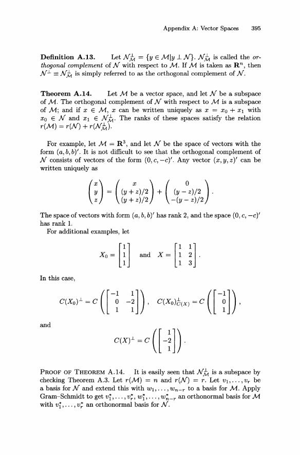
Definition A.13. Let NJA = {y E Mly J..N}. NJA is called the orthogonal complement of N with respect to M. If M is taken as R n , then N 1. == N JA is simply referred to as the orthogonal complement of N.
Theorem A.14. Let M be a vector space, and let N be a subspace of M. The orthogonal complement of N with respect to M is a subspace of Mj and if x E M, x can be written uniquely as x = Xo + Xl with Xo E N and Xl E N JA. The ranks of these spaces satisfy the relation r(M) = r(N) + r(NJA).
For example, let M = R 3 , and let N be the space of vectors with the form (a, b, b)'. It is not difficult to see that the orthogonal complement of N consists of vectors of the form (0, c, -c)'. Any vector (x, y, z)' can be written uniquely as
( :) = ((y :Z)/2) + ( (y _OZ)/2 ) . Z (y + z)/2 -(y - z)/2
The space of vectors with form (a, b, b)' has rank 2, and the space (0, c, -c)' has rank 1.
For additional examples, let
In this case,
and
PROOF OF THEOREM A.14. It is easily seen that N JA is a subspace by checking Theorem A.3. Let r(M) = nand r(N) = r. Let VI,.'" vr be a basis for N and extend this with WI, ... ,Wn - r to a basis for M. Apply Gram-Schmidt to get vi, ... , V;, wi, ... , w~_r an orthonormal basis for M with vi, ... , v; an orthonormal basis for N.

396 Appendix A: Vector Spaces
If x E M, then
r n-r
X = LO!iV; + Lj3jW;. i=l j=l
Let Xo = 2:;=1 O!ivi and Xl = 2:;:::; j3jW;. Then Xo E N, Xl E N ~, and X = Xo + Xl.
To establish the uniqueness of the representation and the rank relationship, we need to establish that {wi, ... , w~_r} is a basis for N ~. Since, by construction, the w;s are linearly independent and w; E N~, j = 1, ... , n - r, it suffices to show that {wi, ... , w~_r} is a spanning set for N~. If X E N~, write
r n-r
X = L O!iV; + L j3jW; . i=l j=l
However, since x E N~ and v'k EN for k = 1, ... , r,
0= x'v'k
r n-r
L O!iV;'V'k + L j3jWi'v'k i=l j=l
O!kV'k'v'k = O!k
for k = 1, .. . , r. Thus x = 2:;:::; j3jW; implying that {wi, ... , w~_r} is a spanning set and a basis for N ~ .
To establish uniqueness, let x = Yo + Yl with Yo E Nand Y1 E N ~. Then ",r * d ",n-r >: * ",r * + ",n-r >: * B Yo = ui=l 'YiVi an Y1 = Uj=l UjWj ; so x = ui=11iVi uj=l UjWj . Y
the uniqueness of the representation of x under any basis, Ii = O!i and j3j = 8j for all i and j; thus Xo = Yo and Xl = Y1.
Since a basis has been found for each of M, N, and N ~, we have r (M) = n, r(N) = r, and r(N~) = n - r. Thus, r(M) = r(N) + r(N~). 0
Definition A.I5. Let N1 and N2 be vector subspaces. Then the sum of NI and N2 is NI + N2 = {xix = Xl + X2, Xl E N l , X2 E N 2}.
Theorem A.I6. NI +N2 is a vector space and C(A, B) = C(A)+C(B).
Appendix A: Vector Spaces 397
Exercises
Exercise A.I Give a detailed proof of the Gram-Schmidt Theorem.
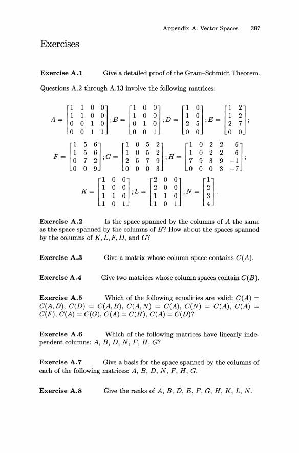
Questions A.2 through A.13 involve the following matrices:
[1 1 0 0] [1 0 0] [1 0] [1 1100 100 10 1
A = 0 0 1 0 jB = 0 1 0 jD = 2 5 jE = 2
0011 001 00 0
5 6] [1 0 5 2] [1 0 2 2 56 1052 1022 7 2 jG= 2 5 7 9 jH= 7 9 3 9
09 0003 0003 -~]j -7
[1 0 0] [2 0 0] [1] 100 200 2
K = 1 1 0 jL = 1 1 0 jN = 3 .
101 101 4
Exercise A.2 Is the space spanned by the columns of A the same as the space spanned by the columns of B? How about the spaces spanned by the columns of K, L, F, D, and G?
Exercise A.3 Give a matrix whose column space contains C(A).
Exercise A.4 Give two matrices whose column spaces contain C(B).
Exercise A.5 Which of the following equalities are valid: C(A) = C(A, D), C(D) = C(A, B), C(A, N) = C(A), C(N) = C(A), C(A) C(F), C(A) = C(G), C(A) = C(H), C(A) = C(D)?
Exercise A.6 Which of the following matrices have linearly inde-pendent columns: A, B, D, N, F, H, G?
Exercise A.7 Give a basis for the space spanned by the columns of each of the following matrices: A, B, D, N, F, H, G.
Exercise A.8 Give the ranks of A, B, D, E, F, G, H, K, L, N.

398 Appendix A: Vector Spaces
Exercise A.9 Which of the following matrices have columns that are mutually orthogonal: B, A, D?
Exercise A.I0 Give an orthogonal basis for the space spanned by the columns of each of the following matrices: A, D, N, K, H, G.
Exercise A.ll Find C(A)J.. and C(B)J.. (with respect to R 4 ).
Exercise A.12 Find two linearly independent vectors in the orthog-onal complement of C(D) (with respect to R 4).
Exercise A.lS Find a vector in the orthogonal complement of C(D) with respect to C(A).
Exercise A.14 the columns of
Find an orthogonal basis for the space spanned by
X=
114 121 1 3 0 140 1 5 1 164
Exercise A.IS For X as above, find two linearly independent vectors in the orthogonal complement of C(X) (with respect to R 6 ).
Exercise A.16 Let X be an n x p matrix. Prove or disprove the following statement: every vector in Rn is in either C(X) or C(X)J.. or both.
Exercise A.17 For any matrix A, prove that C(A) and the null space of A' are orthogonal complements. Note: The null space is defined in Definition B.ll.
Appendix B: Matrix Results
This appendix reviews standard ideas in matrix theory with emphasis given to important results that are less commonly taught in a junior/senior level linear algebra course. The appendix begins with basic definitions and results. A section devoted to eigenvalues and their applications follows. This section contains a number of standard definitions, but it also contains a number of very specific results that are unlikely to be familiar to people with only an undergraduate background in linear algebra. The third section is devoted to an intense (brief but detailed) examination of projections and their properties. The appendix closes with some miscellaneous results, some results on Kronecker products and Vec operators, and an introduction to tensors.
B.l Basic Ideas
Definition B.1. Any matrix with the same number of rows and columns is called a square matrix.
Definition B.2. Let A = [aij] be a matrix. The transpose of A, written A', is the matrix A' = [biJl, where bij = aji.
Definition B.3. If A = A', then A is called symmetric. Note that only
400 Appendix B: Matrix Results
square matrices can be symmetric.
Definition B.4. If A = [aij] is a square matrix and aij = 0 for i =F j, then A is a diagonal matrix. If AI, ... , An are scalars, then D(Aj) and Diag(Aj) are used to indicate an n x n matrix D = [dij ] with dij = 0 i =F j and dii = Ai. If A == (Al, ... ,An)" then D(A) == D(Aj). A diagonal matrix with allIs on the diagonal is called an identity matrix and is denoted I. Occasionally, In is used to denote an n x n identity matrix.
If A = [aij] is nxp and B = [bij ] is nxq, we can write an nx (p+q) matrix G = [A, BJ, where Cij = aij, i = 1, ... , n, j = 1, ... ,p and Cij = bi,j_p, i = 1, ... ,n, j = p+ 1, ... ,p+q. This notation can be extended in obvious
ways, e.g., G' = [~:].
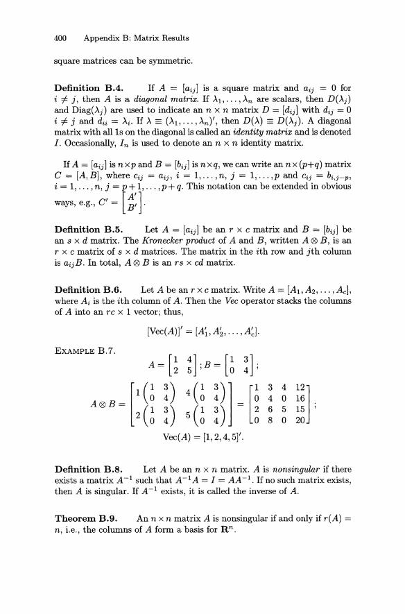
Definition B.5. Let A = [aij] be an r x C matrix and B = [bij ] be an s x d matrix. The Kronecker product of A and B, written A ® B, is an r x c matrix of s x d matrices. The matrix in the ith row and jth column is aij B. In total, A ® B is an r s x cd matrix.
Definition B.6. Let A be an r x c matrix. Write A = [AI, A2 , ••• , Ad, where Ai is the ith column of A. Then the Vec operator stacks the columns of A into an rc x 1 vector; thus,
[Vec(A)]' = [A~,A~, ... ,A~].
EXAMPLE B. 7.
A= [; :];B=[~ !]; [1(~ !) 40 !)]_ [~ 3 4 12]
A®B= 4 0 16
2 (1 3) 5 (1 3) - 2 6 5 15 ' o 4 0 4 0 8 0 20
Vec(A) = [1,2,4,5]'.
Definition B.S. Let A be an n x n matrix. A is nonsingular ifthere exists a matrix A-I such that A-I A = I = AA -1. If no such matrix exists, then A is singular. If A-I exists, it is called the inverse of A.
Theorem B.9. An n x n matrix A is nonsingular if and only if r(A) = n, i.e., the columns of A form a basis for R n.
Corollary B.IO. such that Ax = o.
B.2 Eigenvalues and Related Results 401
Anxn is singular if and only if there exists x =f 0
For any matrix A, the set of all x such that Ax = 0 is easily seen to be a vector space.
Definition B.ll. The set of all x such that Ax = 0 is called the null space of A.
Theorem B.12. If A is n x nand r(A) = r, then the rank of the null space of A is n - r.
B.2 Eigenvalues and Related Results
The material in this section deals with eigenvalues and eigenvectors either in the statements of the results or in their proofs. Again, this is meant to be a brief review of important concepts; but in addition, there are a number of specific results that may be unfamiliar.
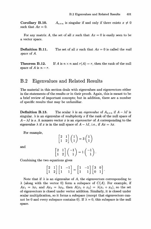
Definition B.13. The scalar A is an eigenvalue of Anxn if A - AI is singular. A is an eigenvalue of multiplicity s if the rank of the null space of A - AI is s. A nonzero vector x is an eigenvector of A corresponding to the eigenvalue A if x is in the null space of A - AI, i.e., if Ax = AX.
For example,
and
Combining the two equations gives
[2 1] [1 -1] = [1 -1] [3 0] 12111101· Note that if A is an eigenvalue of A, the eigenvectors corresponding to
A (along with the vector 0) form a subspace of C(A). For example, if AXl = AXl and AX2 = AX2, then A(Xl + X2) = A(Xl + X2), so the set of eigenvectors is closed under vector addition. Similarly, it is closed under scalar multiplication, so it forms a subspace (except that eigenvectors cannot be 0 and every subspace contains 0). If A = 0, this subspace is the null space.
402 Appendix B: Matrix Results
If A is a symmetric matrix, and "( and A are distinct eigenvalues, then the eigenvectors corresponding to A and "( are orthogonal. To see this, let x be an eigenvector for A and y an eigenvector for "(. Then AX' y = x' Ay = "(x' y, which can happen only if A = "( or if x'y = O. Since A and "( are distinct, we have x'y = o.
Let A1. .. . ,Ar be the distinct nonzero eigenvalues of a symmetric matrix A with respective multiplicities 8(1), ... , 8(r). Let Vil, ... , Vis(i) be a basis for the space of eigenvectors of Ai. We want to show that Vn, VI2,·.·, Vrs(r) is a basis for C(A). Suppose Vn, V12, ... ,Vrs(r) is not a basis. Since Vij E
C(A) and the VijS are linearly independent, we can pick x E C(A) with x .1. Vij for all i and j. Note that since AVij = AiVij, we have (A)PVij = (Ai)PVij . In particular, x'(A)PVij = X'(Ai)PVij = (Ai)PX'Vij = 0, so APx .1. Vij for any i,j, and p. The vectors x, Ax, A2x, ... cannot all be linearly independent, so there exists a smallest value k ~ n such that
Since there is a solution to this, for some real number J1, we can write the equation as
and J1, is an eigenvalue. (See Exercise B.!.) An eigenvector for J1, is y = Ak- 1x + "(k_2Ak-2X + ... + "(ox. Clearly, y .1. Vij for any i and j. Since k was chosen as the smallest value to get linear dependence, we have y =j:. o. If J1, =j:. 0, Y is an eigenvector that does not correspond to any of A1. ... ,An a contradiction. If J1, = 0, we have Ay = OJ and since A is symmetric, y is a vector in C(A) that is orthogonal to every other vector in C(A), i.e., y'y = 0 but y =j:. 0, a contradiction. We have proven
Theorem B.14. If A is a symmetric matrix, then there exists a basis for C(A) consisting of eigenvectors of nonzero eigenvalues. If A is a nonzero eigenvalue of multiplicity 8, then the basis will contain 8 eigenvectors for A.
If A is an eigenvalue of A with multiplicity 8, then we can think of A as being an eigenvalue 8 times. With this convention, the rank of A is the number of nonzero eigenvalues. The total number of eigenvalues is n if A is an n x n matrix.
For a symmetric matrix A, if we use eigenvectors corresponding to the zero eigenvalue, we can get a basis for R n consisting of eigenvectors. We already have a basis for C (A), and the eigenvectors of 0 are the null space of A. For A symmetric, C(A) and the null space of A are orthogonal complements. Let AI, ... ,An be the eigenvalues of a symmetric matrix A. Let
B.2 Eigenvalues and Related Results 403
VI, ... , Vn denote a basis of eigenvectors for R n, with Vi being an eigenvector for Ai for any i.
Theorem B.I5. If A is symmetric, there exists an orthonormal basis for R n consisting of eigenvectors of A.
PROOF. Assume Ail = ... = Aik are all the AiS equal to any particular value A, and let ViI, ... , vik be a basis for the space of eigenvectors for A. By Gram-Schmidt there exists an orthonormal basis Wil, .•. , Wik for the space of eigenvectors corresponding to A. If we do this for each distinct eigenvalue, we get a collection of orthonormal sets that form a basis for Rn. Since, as we have seen, for Ai =1= Aj, any eigenvector for Ai is orthogonal to any eigenvector for Aj, the basis is orthonormal. 0
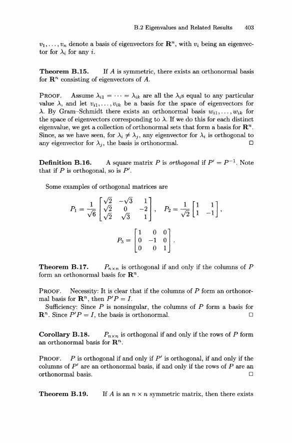
Definition B.I6. A square matrix P is orthogonal if pI = p-I. Note that if P is orthogonal, so is P'.
Some examples of orthogonal matrices are
-J3 1] o -2, J3 1
Theorem B.I7. Pnxn is orthogonal if and only if the columns of P form an orthonormal basis for R n.
PROOF. Necessity: It is clear that if the columns of P form an orthonormal basis for Rn, then pIp = I.
Sufficiency: Since P is nonsingular, the columns of P form a basis for Rn. Since pIp = I, the basis is orthonormal. 0
Corollary B.IS. Pnxn is orthogonal if and only if the rows of P form an orthonormal basis for R n .
PROOF. P is orthogonal if and only if pI is orthogonal, if and only if the columns of pI are an orthonormal basis, if and only if the rows of P are an orthonormal basis. 0
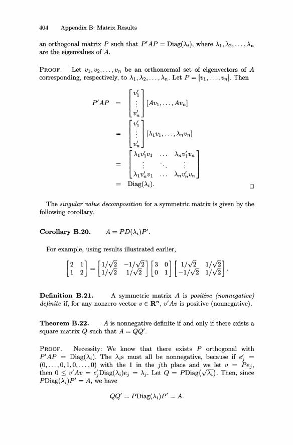
Theorem B.I9. If A is an n x n symmetric matrix, then there exists
404 Appendix B: Matrix Results
an orthogonal matrix P such that pI AP = Diag(Ai), where AI, A2,"" An are the eigenvalues of A.
PROOF. Let VI, V2, •.. ,Vn be an orthonormal set of eigenvectors of A corresponding, respectively, to AI. A2,' .. ,An. Let P = [VI, ... ,vnJ. Then
P'AP =
[ Al~iVl AlV~Vl
= Diag(Ai). o
The singular value decomposition for a symmetric matrix is given by the following corollary.
Corollary B.20.
For example, using results illustrated earlier,
[2 1] = [1/v'2 -1/v'2] [3 0] [1/v'2 1/v'2] 1 2 1/v'2 1/v'2 ° 1 -1/v'2 1/v'2 .
Definition B.21. A symmetric matrix A is positive (nonnegative) definite if, for any nonzero vector v ERn, v' Av is positive (nonnegative).
Theorem B.22. A is nonnegative definite if and only if there exists a square matrix Q such that A = QQ'.
PROOF. Necessity: We know that there exists P orthogonal with pI AP = Diag(Ai). The AiS must all be nonnegative, because if ej = (0, ... ,0,1,0, ... ,0) with the 1 in the jth place and we let v = Pej, then ° ::; v' Av = ejDiag(Ai)ej = Aj. Let Q = PDiag( A). Then, since PDiag(Ai)P' = A, we have
QQ' = PDiag(Ai)P' = A.
B.2 Eigenvalues and Related Results 405
Sufficiency: If A = QQ', then v' Av = (Q'v)'(Q'v) 2: O. 0
Corollary B.23. A is positive definite if and only if Q is nonsingular for any choice of Q.
PROOF. There exists v i' 0 such that v' Av = 0 if and only if there exists v i' 0 such that Q'v = 0, which occurs if and only if Q' is singular. The contrapositive of this is that v' Av > 0 for all v i' 0 if and only if Q' is nonsingular. 0
Theorem B.24. If A is an n x n nonnegative definite matrix with nonzero eigenvalues Al,"" Ar , then there exists an n x r matrix Q = Q1Q"2l such that Ql has orthonormal columns, C(Ql) = C(A), Q2 is diagonal and nonsingular, and Q' AQ = I.
PROOF. Let Vl,"" Vn be an orthonormal basis of eigenvectors with Vl, ... , Vr corresponding to Al,"" Ar· Let Ql = [Vl, ... , vr]. By an argument similar to that in the proof of Theorem B.19, Q~AQl = Diag(Ai), i = 1, ... ,r. Now take Q2 = Diag(A) and Q = Q1Q"2l. 0
Corollary B.25.
PROOF. Since Q'AQ = Q"21Q~AQ1Q"2l = I and Q2 is symmetric, Q~AQl = Q2Q~. Multiplying gives
Q1Q~AQ1Q~ = (Q1Q2)(Q~QD = WW'.
But Q1Q~ is a perpendicular projection matrix onto C(A), so Q1Q~AQ1Q~ = A (cf. Definition B.31 and Theorem B.35). 0
Corollary B.26. AQQ' A = A and QQ' AQQ' = QQ'.
PROOF. AQQ'A = WW'QQ'WW' = WQ2Q~Q1Q"21Q"21Q~Q1Q2W' = A. QQ'AQQ' = QQ'WW'QQ' = QQ"21Q~Q1Q2Q2Q~Q1Q21Q' = QQ'. 0
Definition B.27. tr(A) = E~=l aii'
Let A = [aij] be an n x n matrix. The trace of A is
Theorem B.2B. For matrices Arxs and Bsxn tr(AB) = tr(BA).
PROOF. See Exercise B.8. o
Theorem B.29. If A is a symmetric matrix, tr(A) = E~=l Ai, where Al, ... ,An are the eigenvalues of A.
406 Appendix B: Matrix Results
PROOF. A = PD(>"i)P' with P orthogonal
tr(A) tr(P D(>"i)P') = tr(D(>"i)P' P) n
tr(D(>"i)) = L >"i. o i=l
To illustrate, we saw earlier that the matrix [i ;] had eigenvalues of
3 and 1. In fact, a stronger result than Theorem B.29 is true. We give it without proof.
Theorem B.30. of A.
tr(A) = 2::~=1 >"i, where >"1, ... ,>"n are the eigenvalues
B.3 Projections
This section is devoted primarily to a discussion of perpendicular projection operators. It begins with their definition, some basic properties, and two important characterizations: Theorems B.33 and B.35. A third important characterization, Theorem B.44, involves generalized inverses. Generalized inverses are defined, briefly studied, and applied to projection operators. The section continues with the examination of the relationships between two perpendicular projection operators and closes with discussions of the Gram-Schmidt theorem, eigenvalues of projection operators, and oblique (nonperpendicular) projection operators.
We begin by defining a perpendicular projection operator onto an arbitrary space. To be consistent with later usage, we denote the arbitrary space C(X) for some matrix X.
Definition B.3!. M is a perpendicular projection operator (matrix) onto C (X) if and only if
(i) v E C(X) implies Mv = v (projection)
(ii) w 1- C(X) implies Mw = 0 (perpendicularity).
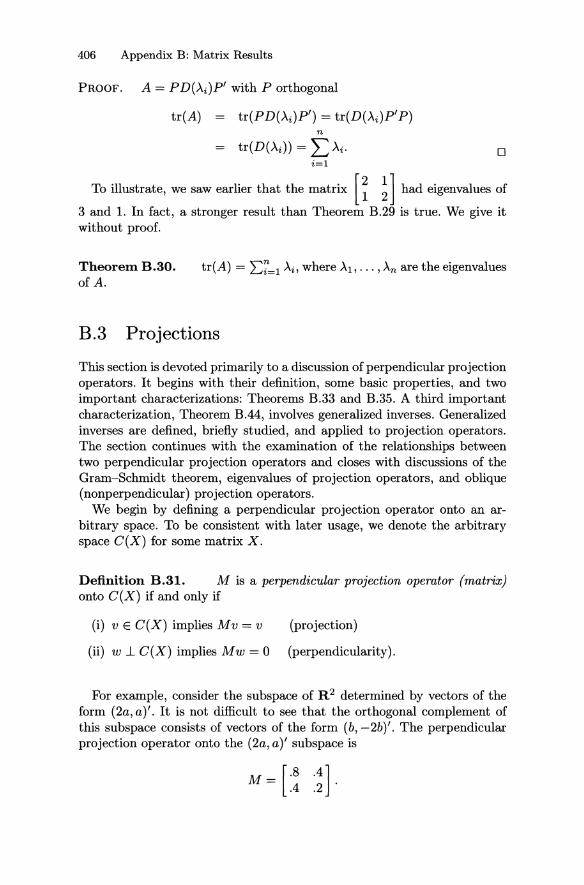
For example, consider the subspace of R 2 determined by vectors of the form (2a, a)'. It is not difficult to see that the orthogonal complement of this subspace consists of vectors of the form (b, -2b)'. The perpendicular projection operator onto the (2a, a)' subspace is
M = [.8 .4] . .4 .2
B.3 Projections 407
To verify this note that
M(2a) = [.8 .4] (2a) = ((.8)2a+.4a) = (2a) a .4.2 a (.4)2a + .2a a
and
M( b) [.8.4] ( b) (.8b+.4(-2b)) (0) -2b = .4.2 -2b = .4b+.2(-2b) = 0 .
Proposition B.32. If M is a perpendicular projection operator onto C(X), then C(M) = C(X).
PROOF. See Exercise B.2. o
Note that both columns of
M = [.8 .4] .4 .2
have the form (2a, a)'.
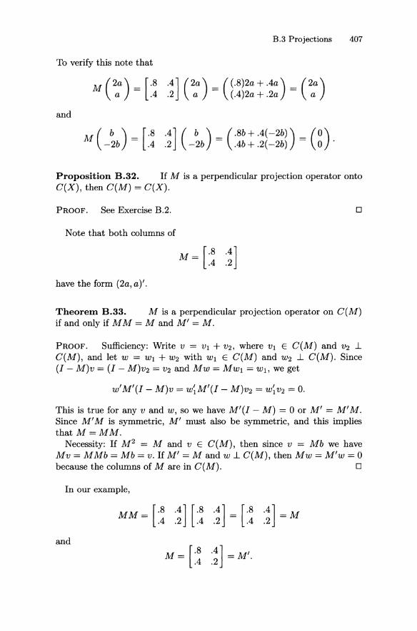
Theorem B.33. M is a perpendicular projection operator on C(M) if and only if MM = M and M' = M.
PROOF. Sufficiency: Write v = VI + V2, where VI E C(M) and V2 .1 C(M), and let W = WI + W2 with WI E C(M) and W2 .1 C(M). Since (I - M)v = (I - M)V2 = V2 and Mw = MWI = WI, we get
w'M'(I - M)v = w~M'(I - M)V2 = W~V2 = O.
This is true for any V and w, so we have M'(I - M) = 0 or M' = M'M. Since M'M is symmetric, M' must also be symmetric, and this implies that M=MM.
Necessity: If M2 = M and v E C(M), then since v = Mb we have Mv = MMb = Mb = v. If M' = M and w.l C(M), then Mw = M'w = 0 because the columns of M are in C(M). 0
In our example,
M M = [:~ :~] [:~ :~] = [:~ :~] = M
and
M = [.8 .4] = M' . . 4 .2
408 Appendix B: Matrix Results
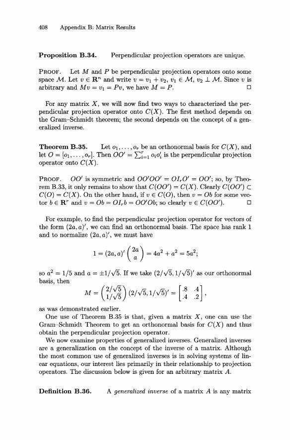
Proposition B.34. Perpendicular projection operators are unique.
PROOF. Let M and P be perpendicular projection operators onto some space M. Let vERn and write v = VI + V2, VI E M, V2 ..L M. Since v is arbitrary and Mv = VI = Pv, we have M = P. 0
For any matrix X, we will now find two ways to characterized the perpendicular projection operator onto C(X). The first method depends on the Gram-Schmidt theorem; the second depends on the concept of a generalized inverse.
Theorem B.35. Let 01, .•. , Or be an orthonormal basis for C(X), and let 0 = [01, •.• , Or]. Then 00' = E~=l OiO~ is the perpendicular projection operator onto C(X).
PROOF. 00' is symmetric and 00'00' = OIrO' = 00'; so, by Theorem B.33, it only remains to show that C(OO') = C(X). Clearly C(OO') c C(O) = C(X). On the other hand, if V E C(O), then v = Ob for some vector bE R r and v = Ob = OIrb = OO'Ob; so clearly v E C(OO'). 0
For example, to find the perpendicular projection operator for vectors of the form (2a, a)', we can find an orthonormal basis. The space has rank 1 and to normalize (2a,a)', we must have
so a2 = 1/5 and a = ±1/v'5. If we take (2/v'5, 1/v'5)' as our orthonormal basis, then
as was demonstrated earlier. One use of Theorem B.35 is that, given a matrix X, one can use the
Gram-Schmidt Theorem to get an orthonormal basis for C(X) and thus obtain the perpendicular projection operator.
We now examine properties of generalized inverses. Generalized inverses are a generalization on the concept of the inverse of a matrix. Although the most common use of generalized inverses is in solving systems of linear equations, our interest lies primarily in their relationship to projection operators. The discussion below is given for an arbitrary matrix A.
Definition B.36. A generalized inverse of a matrix A is any matrix

B.3 Projections 409
G such that AGA = A. The notation A- is used to indicate a generalized inverse of A.
Theorem B.37. A is A-l.
If A is nonsingular, the unique generalized inverse of
PROOF. AA-l A = IA = A, so A-l is a generalized inverse. If AA-A = A, then AA- = AA-AA-l = AA-l = Ij so A- is the inverse of A. 0
Theorem B.3S. ized inverse of A.
For any symmetric matrix A, there exists a general-
PROOF. There exists P orthogonal so that P' AP = D(Ai) and A = PD(Ai)P'. Let
. _ { 1/ Ai if An.f 0 '"Y. - 0 if Ai = 0 '
and G = PD("(i)P'. We now show that G is a generalized inverse of A. P is orthogonal, so P' P = I and
AGA PD(Ai)P'PD("Yi)P'PD(Ai)P'
= P D(Ai)D( '"Yi)D(Ai)P'
= PD(Ai)P'
A. o
Although this is the only existence result we really need, later we will show that generalized inverses exist for arbitrary matrices.
Theorem B.39. is G1AG2 .
If G1 and G2 are generalized inverses of A, then so
o
For A symmetric, A-need not be symmetric.
EXAMPLE B.40. Consider the matrix
It has a generalized inverse
[1/a -1] 1 0 '
410 Appendix B: Matrix Results
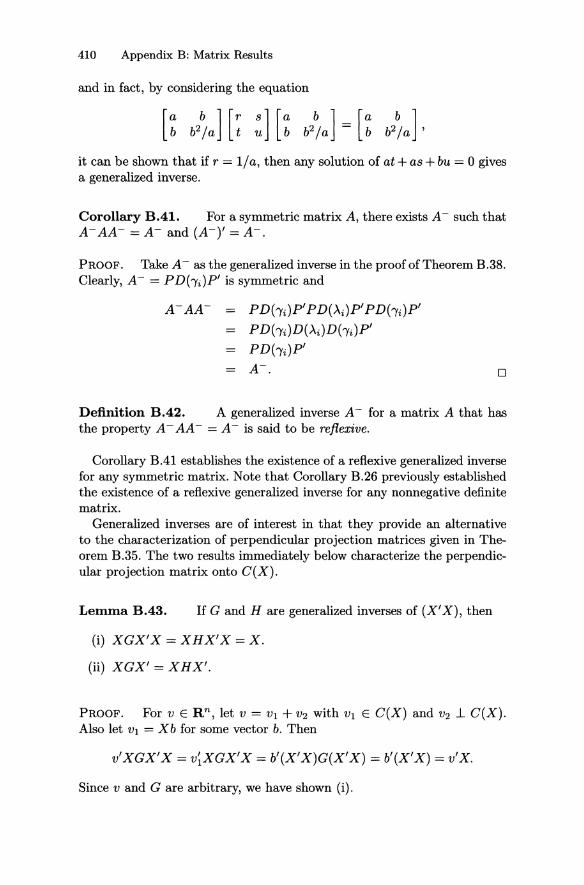
and in fact, by considering the equation
it can be shown that if r = 1/ a, then any solution of at + as + bu = 0 gives a generalized inverse.
Corollary B.41. For a symmetric matrix A, there exists A-such that A-AA- = A- and (A-), = A-.
PROOF. Take A- as the generalized inverse in the proof of Theorem B.38. Clearly, A- = PDbi}P' is symmetric and
A-AA- = P D( "Ii}P' P D(A.i}P' P D( "Ii}P'
= P DC "Ii}D(A.i}D( "Ii}P'
= PDbi}P'
= A-. a
Definition B.42. A generalized inverse A-for a matrix A that has the property A - AA - = A-is said to be reflexive.
Corollary B.41 establishes the existence of a reflexive generalized inverse for any symmetric matrix. Note that Corollary B.26 previously established the existence of a reflexive generalized inverse for any nonnegative definite matrix.
Generalized inverses are of interest in that they provide an alternative to the characterization of perpendicular projection matrices given in Theorem B.35. The two results immediately below characterize the perpendicular projection matrix onto C(X}.
Lemma B.43. If G and H are generalized inverses of (X' X), then
(i) XGX'X=XHX'X=X.
(ii) XGX' = XHX'.
PROOF. For vERn, let v = Vl + V2 with Vl E C(X} and V2 .1 C(X}. Also let Vl = Xb for some vector b. Then
v'XGX'X = v~XGX'X = b'(X'X}G(X'X} = b'(X'X} = v'x.
Since v and G are arbitrary, we have shown (i).
B.3 Projections 411
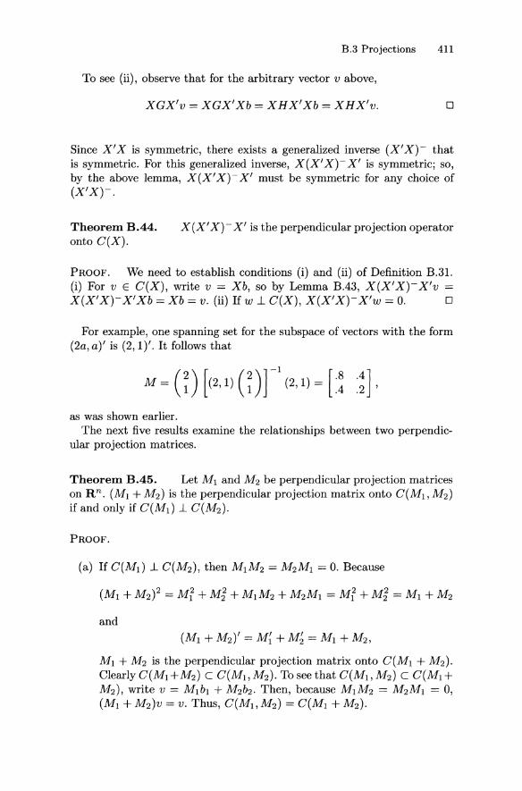
To see (ii), observe that for the arbitrary vector v above,
XGX'v = XGX'Xb = XHX'Xb = XHX'v. o
Since X' X is symmetric, there exists a generalized inverse (X' X) - that is symmetric. For this generalized inverse, X(X'X)- X' is symmetric; so, by the above lemma, X(X' X)- X' must be symmetric for any choice of (X'X)-.
Theorem B.44. onto G(X).
X(X' X)- X' is the perpendicular projection operator
PROOF. We need to establish conditions (i) and (ii) of Definition B.31. (i) For v E G(X), write v = Xb, so by Lemma B.43, X(X'X)-X'v = X(X' X)-X' Xb = Xb = v. (ii) If w ..L G(X), X(X' X)- X'w = O. 0
For example, one spanning set for the subspace of vectors with the form (2a, a)' is (2,1)'. It follows that
as was shown earlier. The next five results examine the relationships between two perpendic
ular projection matrices.
Theorem B.45. Let Ml and M2 be perpendicular projection matrices on Rn. (Ml + M 2 ) is the perpendicular projection matrix onto G(M!, M 2) if and only if G(Md ..L G(M2)'
PROOF.
and
(Ml + M 2)' = M{ + M~ = Ml + M 2,
Ml + M2 is the perpendicular projection matrix onto G(Ml + M2)' Clearly G(Ml +M2) c G(M!, M 2). To see that G(M!, M 2) c G(Ml + M 2), write v = Mlbl + M 2b2. Then, because MlM2 = M2Ml = 0, (Ml + M 2)v = v. Thus, G(Mb M 2) = G(Ml + M2)'
412 Appendix B: Matrix Results
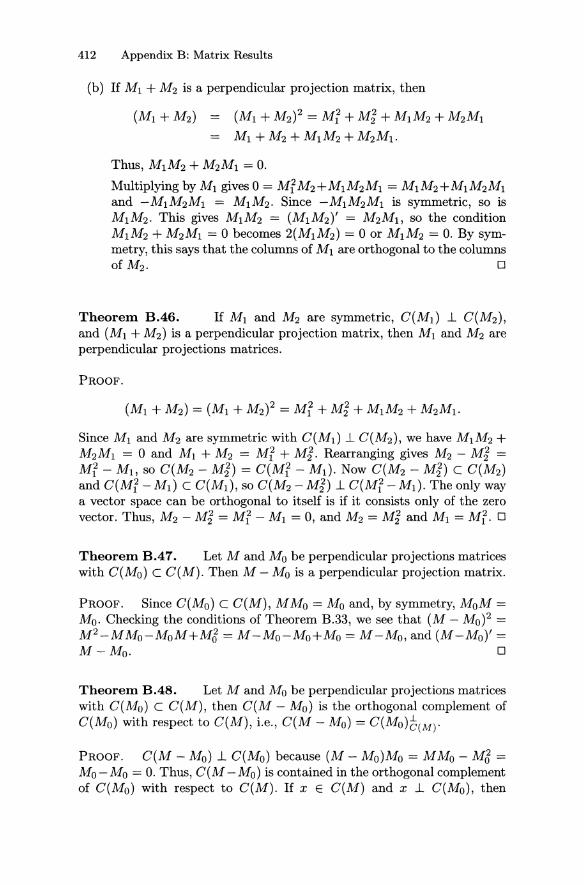
(b) If Ml + M2 is a perpendicular projection matrix, then
(Ml + M2) = (Ml + M2)2 = M'f + M~ + MIM2 + M2Ml
MI + M2 + MIM2 + M2M1 .
Thus, MIM2 + M2MI = O.
Multiplying by MI gives 0 = M'f M2+MIM2MI = MIM2+MIM2MI and -MIM2MI = MIM2. Since -MIM2Ml is symmetric, so is MIM2. This gives MIM2 = (MIM2)' = M2M}, so the condition MIM2 + M2Ml = 0 becomes 2(MIM2) = 0 or MIM2 = O. By symmetry, this says that the columns of MI are orthogonal to the columns ~~. 0
Theorem B.46. If MI and M2 are symmetric, C(MI) -L C(M2), and (MI + M2) is a perpendicular projection matrix, then MI and M2 are perpendicular projections matrices.
PROOF.
Since MI and M2 are symmetric with C(M1 ) -L C(M2), we have MIM2 + M2Ml = 0 and Ml + M2 = M[ + M? Rearranging gives M2 - M? = M[ - MI , so C(M2 - M?) = C(M[ - Md. Now C(M2 - M?) c C(M2) and C(M[ - M1 ) c C(M1 ), so C(M2 - M?) -L C(M[ - Ml)' The only way a vector space can be orthogonal to itself is if it consists only of the zero vector. Thus, M2 - M? = M[ - Ml = 0, and M2 = M? and Ml = Mf. 0
Theorem B.47. Let M and Mo be perpendicular projections matrices with C(Mo) C C(M). Then M - Mo is a perpendicular projection matrix.
PROOF. Since C(Mo) C C(M), MMo = Mo and, by symmetry, MoM = Mo. Checking the conditions of Theorem B.33, we see that (M - MO)2 = M2_MMo-MoM+M6 = M-Mo-Mo+Mo = M-Mo, and (M-Mo)' = M-~. 0
Theorem B.4S. Let M and Mo be perpendicular projections matrices with C(Mo) C C(M), then C(M - Mo) is the orthogonal complement of C(Mo) with respect to C(M), Le., C(M - Mo) = C(MO)~(M)'
PROOF. C(M - Mo) -L C(Mo) because (M - Mo)Mo = MMo - M6 = Mo-Mo = O. Thus, C(M -Mo) is contained in the orthogonal complement of C(Mo) with respect to C(M). If x E C(M) and x -L C(Mo), then
B.3 Projections 413
x = Mx = (M - Mo)x + Mox = (M - Mo)x. Thus, X E C(M - Mo), so the orthogonal complement of C(Mo) with respect to C(M) is contained in C(M - Mo). 0
Corollary B.49. r(M) = r(Mo) + r(M - Mo).
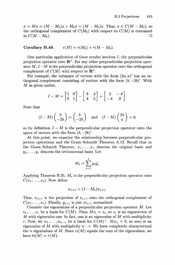
One particular application of these results involves I, the perpendicular projection operator onto Rn. For any other perpendicular projection operator M, I -M is the perpendicular projection operator onto the orthogonal complement of C(M) with respect to Rn.
For example, the subspace of vectors with the form (2a, a)' has an orthogonal complement consisting of vectors with the form (b, -2b)'. With M as given earlier,
I-M= [1 0] _ [.8 .4] = [.2 ° 1 .4.2 -.4 -.4] .8 .
Note that
so by definition I - M is the perpendicular projection operator onto the space of vectors with the form (b, -2b)'.
At this point, we examine the relationship between perpendicular projection operations and the Gram-Schmidt Theorem A.12. Recall that in the Gram-Schmidt Theorem, Xl, ... , xr denotes the original basis and Yl, ... ,Yr denotes the orthonormal basis. Let
s
Ms = LYiY~. i=l
Applying Theorem B.35, Ms is the perpendicular projection operator onto C(Xl. ... ,xs). Now define
Thus, W s+! is the projection of X s+! onto the orthogonal complement of C(Xl. . .. ,xs). Finally, Ys+! is just W s+! normalized.
Consider the eigenvalues of a perpendicular projection operator M. Let Vl, ... ,Vr be a basis for C (M). Then M Vi = Vi, so Vi is an eigenvector of M with eigenvalue one. In fact, one is an eigenvalue of M with multiplicity r. Now, let Wl, ... ,Wn - r be a basis for C(M)-L. MWj = 0, so zero is an eigenvalue of M with multiplicity n - r. We have completely characterized the n eigenvalues of M. Since tr(M) equals the sum of the eigenvalues, we have tr(M) = r(M).
414 Appendix B: Matrix Results
In fact, if A is an n x n matrix with A2 = A, any basis for C(A) is a basis for the space of eigenvectors for the eigenvalue 1. The null space of A is the space of eigenvectors for the eigenvalue O. The rank of A and the rank of the null space of A add to n, and A has n eigenvalues, so all the eigenvalues are accounted for. Again, tr(A) = r(A).
Definition B.50.
(a) If A is a square matrix with A2 = A, then A is called idempotent.
(b) Let Nand M be two spaces withNnM = {O} and r(N)+r(M) = n. The square matrix A is a projection operator onto N along M if (1) Av = v for any v EN and (2) Aw = 0 for any w E M.
If the square matrix A has the property that Av = v for any v E C(A), then A is the projection operator (matrix) onto C(A) along C(A')1-. (Note that C(A').L is the null space of A.) It follows immediately that if A is idempotent, then A is a projection operator onto C(A) along N(A) = C(A').L.
The uniqueness of projection operators can be established like it was for perpendicular projection operators. Note that x E Rn can be written uniquely as x = v + w for v E Nand w E M. To see this, take basis matrices for the two spaces, say N and M, respectively. The result follows from observing that [N, M] is a basis matrix for Rn. Because of the rank conditions, [N, M] is an n x n marix. It is enough to show that the columns
of [N,M] must be linearly independent. 0 = [N,M] [~] = Nb + Me
implies Nb = M( -c) which, since N n M = {O}, can only happen when Nb = 0 = M( -e), which, because they are basis matrices, can only happen
when b = 0 = (-c), which implies that [~] = 0, and we are done.
Any projection operator that is not a perpendicular projection is referred to as an oblique projection opemtor.
To show that a matrix A is a projection operator onto an arbitrary space, say C(X), it is necessary to show that C(A) = C(X) and that for x E C(X), Ax = x. A typical proof runs in the following pattern. First show that Ax = x for any x E C(X). This also establishes that C(X) c C(A). To finish the proof, it suffices to show that Av E C(X) for any vERn because this implies that C(A) c C(X).
In this book, our use of the word "perpendicular" is based on using the standard inner product, which defines Euclidean distance. In other words, for two vectors x and y, their inner product is x'y. By definition, the vectors x and yare orthogonal if their inner product is zero. The length of a vector x is defined as the square root of the inner product of x with itself, i.e.,
B.4 Miscellaneous Results 415
IIxll == M. These concepts can be generalized. For a positive definite matrix B, we can define an inner product between x and y as x' By. As before, x and yare orthogonal if their inner product is zero and the length of x is the square root of its inner product with itself (now IIxllB == v'x' Bx). As argued above, any idempotent matrix is always a projection operator, but which one is the perpendicular projection operator depends on the inner product. As can be seen from Proposition 2.7.2 and Exercise 2.5, the matrix X(X' BX)- X' B is an oblique projection onto C(X) for the standard inner product; but it is the perpendicular projection operator onto C(X) with the inner product defined using the matrix B.
B.4 Miscellaneous Results
Proposition B.51. For any matrix X, C(XX') = C(X).
PROOF. Clearly C(XX') C C(X), so we need to show that C(X) C C(XX'). Let x E C(X). Then x = Xb for some b. Write b = bo + b1, where bo E C(X') and b1 ..L C(X'). Clearly, Xb1 = 0, so we have x = Xbo. But bo = X'd for some d; so x = Xbo = XX'd and x E C(XX'). 0
Corollary B.52. For any matrix X, r(XX') = r(X).
PROOF. See Exercise B.4. o
Corollary B.53. is nonsingular.
If X nxp has r(X) = p, then the p x p matrix X' X
PROOF. See Exercise B.5. o
Proposition B.54. If B is nonsingular, C(XB) = C(X).
PROOF. Clearly, C(XB) C C(X). To see that C(X) C C(XB), take x E C(X). It follows that for some vector b, x = Xb; so x = XB(B-1b) E C(XB). 0
It follows immediately from Proposition B.54 that the perpendicular projection operators onto C(XB) and C(X) are identical.
We now show that generalized inverses always exist.
Theorem B.55. X-.
For any matrix X, there exists a generalized inverse
416 Appendix B: Matrix Results
PROOF. We know that (X'X)- exists. Set X- = (X'X)-X'. Then XX-X = X(X'X)-X'X = X because X(X'X)-X' is a projection matrix onto C(X). 0
Proposition B.56. When all inverses exist, [A + BCDr1 = A-I -A-1B [C-1 +DA-1Br1 DA-1.
PROOF.
[A + BCD] [A-1 - A-I B [C-1 + DA-1 Br1 DA-1]
1- B [C- I + DA-I B] -1 DA-I + BCDA-I
-BCDA-IB [C- I +DA-IBr l DA-1
1- B [I + CDA-IB] [C-1 + DA-1 Brl DA-I + BCDA-I
1- BC [C-I + DA-IB] [C-1 + DA-IB]-l DA-I + BCDA-I
1- BCDA-I + BCDA-I = I. o
When we consider applications of linear models, we will frequently need to refer to matrices and vectors that consist entirely of Is. Such matrices are denoted by the letter J with various subscripts and superscripts to specify their dimensions. J~ is an r x c matrix of Is. The subscript indicates the number of rows and the superscript indicates the number of columns. If there is only one column, the superscript may be suppressed, e.g., Jr = J;. In a context where we are dealing with vectors in R n, the subscript may also be suppressed, e.g., J = I n = J~.
A matrix of zeros will always be denoted by O.
B.5 Properties of Kronecker Products and Vec Operators
Kronecker products and Vec operators are extremely useful in multivariate analysis and some approaches to variance component estimation. They are also often used in writing down balanced ANOVA models. We now present their basic algebraic properties.
1. If the matrices are of conformable sizes, [A ® (B + C)] = [A ® B] + [A®C].
2. If the matrices are of conformable sizes, [(A + B) ® C] = [A ® C] + [B®C].
3. If a and b are scalars, ab[A ® B] = faA ® bBl.

B.5 Properties of Kronecker Products and Vec Operators 417
4. If the matrices are of conformable sizes, [A®B][C®Dl = [AC®BDl.
5. The generalized inverse of a Kronecker product matrix is [A®Bl- = [A- ®B-l.
6. For two vectors v and w, Vec(vw') = W ® v.
7. For a matrix W and conformable matrices A and B, Vec(AWB') = [B ® AlVec(W).
8. For conformable matrices A and B, Vec(A)'Vec(B) = tr(A' B).
9. The Vec operator commutes with any matrix operation that is performed elementwise. For example, E{Vec(W)} = Vec{E(W)} when W is a random matrix. Similarly, for conformable matrices A and B and scalar ¢, Vec(A+B) = Vec(A) + Vec(B) and Vec(¢A) = ¢Vec(A).
10. If A and B are positive definite, then A ® B is positive definite.
Most of these are well known facts and easy to establish. Two of them are somewhat more unusual and we present proofs.
ITEM 7. We show that for a matrix Wand conformable matrices A and B, Vec(AW B') = [B ® AlVec(W). First note that if Vec(AW) = [I ® AlVec(W) and Vec(WB') = [B ® IlVec(W) , then Vec(AWB') = [I ® AlVec(W B') = [I ® A][B ® IlVec(W) = [B ® AlVec(W).
To see that Vec(AW) = [I ® AlVec(W), let W be r x s and write W in terms of its columns W = [WI, ... ,wsl. Then AW = [AWl, ... ,Awsl and Vec(AW) stacks the columns AWl' ... ' Aws. On the other hand,
[A 0] [WI] [AWl] [I ® AlVec(W) = . . : :.
o A Ws Aws
To see that Vec(WB') = [B ® IlVec(W), take W as above and write Bmxs = [bijl with rows b~, ... ,b~. First note that WB' = [Wbl , ... , Wbm], so Vec(WB') stacks the columns Wbl , ... , Wbm. Now observe that
ITEM 10. To see that if Arxr and Bsxs are positive definite, then A®B is positive definite, consider the eigenvalues and eigenvectors of A and B. Recall that a symmetric matrix is positive definite if and only if all of its

418 Appendix B: Matrix Results
eigenvalues are positive. Suppose that Av = ¢v and Bw = Ow. We now show that all of the eigenvalues of A 0 B are positive. Observe that
[A0B][v0w] [Av 0 Bw]
[¢v 0 Ow]
¢O[v0w].
This shows that [v 0 w] is an eigenvector of [A 0 B] corresponding to the eigenvalue ¢O. As there are r choices for ¢ and s choices for 0, this accounts for all r s of the eigenvalues in the r s x r s matrix [A 0 B]. Moreover, ¢ and o are both positive, so all of the eigenvalues of [A 0 B] are positive.
B.6 Tensors
Tensors are simply an alternative notation for writing vectors. This notation has substantial advantages when dealing with quadratic forms and when dealing with more general concepts than quadratic forms. Our main purpose in discussing them here is simply to illustrate how flexibly subscripts can be used in writing vectors.
Consider a vector Y = (Y1, ... , Yn)'. The tensor notation for this is simply Yi. We can write another vector a = (a1, ... , an)' as ai. When written individually, the subscript is not important. In other words, ai is the same vector as aj. Note that the length of these vectors needs to be understood from the context. Just as when we write Y and a in conventional vector notation, there is nothing in the notation Yi or ai to tell us how many elements are in the vector.
If we want the inner product a'Y, in tensor notation we write aiYi. Here we are using something called the summation convention. Because the subscripts on ai and Yi are the same, aiYi is taken to mean E~=1 aiYi. If, on the other hand, we wrote aiYj, this means something completely different. aiYj is an alternative notation for the Kroneker product [a 0 Y] = (a1Y1, ... , a1Yn, a2Y1,· .. , anYn)'. In [a 0 Y] == aiYj, we have two subscripts identifying the rows of the vector.
Now, suppose we want to look at a quadratic form Y' AY, where Y is an n vector and A is n x n. One way to rewrite this is
n n n n
i=1 j=1 i=1 j=1
Here we have rewritten the quadratic form as a linear combination of the elements in the vector [Y 0 Y]. The linear combination is determined by the elements of the vector Vec(A). In tensor notation, this becomes quite simple. Using the summation convention in which objects with the same
B.6 Tensors 419
subscript are summed over,
The second term just has the summation signs removed, but the third term, which obviously gives the same sum as the second, is actually the tensor notation for Vec(A)'[Y ® Y]. Again, Vec(A) = (all,a2ba31,'" ,ann)' uses two subscripts to identify rows of the vector. Obviously, if you had a need to consider things like
n n n
L L L aijkYiYjYk == aijkYiYjYk, i=l j=l k=l
the tensor version aijkYiYjYk saves some work. There is one slight complication in how we have been writing things.
Suppose A is not symmetric and we have another n vector W. Then we might want to consider
n n
W'AY = LLwiaijYj. i=l j=l
In this case, a little care must be used because
n n n n
i=l j=l i=l j=l
or W'AY = Y'A'W = Vec(A')'[W ® Y]. However, with A nonsymmetric, W' A'Y = Vec(A')'[Y®W] is typically different from W' AY. The Kronecker notation requires that care be taken in specifying the order of the vectors in the Kroneker product, and whether or not to transpose A before using the Vec operator. In tensor notation, W' AY is simply WiaijYj' In fact, the orders of the vectors can be permuted in any way; so, for example, aijYjWi means the same thing. W' A'Y is simply WiajiYj' The tensor notation and the matrix notation require less effort than the Kronecker notation.
For our purposes, the real moral here is simply that the subscripting of an individual vector does not matter. We can write a vector Y = (Yl,"" Yn)' as Y = [Yk] (in tensor notation as simply Yk), or we can write the same n vector as Y = [Yij] (in tensor notation, simply Yij), where, as long as we know the possible values that i and j can take on, the actual order in which we list the elements is not of much importance. Thus if i = 1, ... ,t and j = 1, ... , Ni with n = L::=l N i , it really does not matter if we write a vector Y as (YI,"" Yn), or (Yll,"" YINl , Y21, ... , YtNt )', or (Ytl, ... ,YtNt> Yt-l,b ... ,YINJ', or in any other fashion we may choose, as long as we keep straight which row of the vector is which. Thus, a linear combination a'Y can be written L:~=l akYk or L::=1 L:~l aijYij' In tensor

420 Appendix B: Matrix Results
notation, the first of these is simply akYk and the second is aijYij' These ideas become very handy in examining analysis of variance models, where the standard approach is to use multiple subscripts to identify the various observations. The subscripting has no intrinsic importance; the only thing that matters is knowing which row is which in the vectors. The subscripts are an aid in this identification, but they do not create any problems. We can still put all of the observations into a vector and use standard operations on them.
B.7 Exercises
Exercise B.1
(a) Show that
AkX + bk_IAk-Ix + ... + box =
(A - J.LI) (Ak-Ix + Tk_2Ak-2X + ... + TOX) = 0,
where J.L is any nonzero solution of bo + bl w + ... + bkwk = 0 with bk = 1 and Tj = -(bo + blJ.L + ... + bjJ.Lj)j J.Lj+1, j = 0, ... , k.
(b) Show that if the only root of bo + bIw + ... + bkWk is zero, then the factorization in (a) still holds.
(c) The solution J.L used in (a) need not be a real number, in which case J.L is a complex eigenvalue and the TiS are complex; so the eigenvector is complex. Show that with A symmetric, J.L must be real because the eigenvalues of A must be real. In particular, assume that
A(y + iz) = (>. + i-y)(y + iz),
for Y, z, >., and "'( real vectors and scalars, respectively, set Ay >.y - "'(z, Az = "'(y + >.z, and examine z' Ay = y' Az.
Exercise B.2 Prove Proposition B.32.
Exercise B.3 Show that any nonzero symmetric matrix A can be written as A = PDP', where C(A) = C(P), p'p = I, and D is nonsingu-

B.7 Exercises 421
lar.
Exercise B.4 Prove Corollary B.52.
Exercise B.5 Prove Corollary B.53.
Exercise B.6 Show tr(cIn ) = nco
Exercise B. 7 the inverse of
Let a, b, c, and d be real numbers. If ad - be i= 0, find
[~ ~]. Exercise B.8 Prove Theorem B.28, i.e., let A be an r x s matrix, let B be an s x r matrix, and show that tr(AB) = tr(BA).
Exercise B. 9 Determine whether the matrices given below are positive definite, nonnegative definite, or neither.
[j 2 -2] [26 -2 -7] [26 2 13] [ 3 2 -2] 2 -2 ; -2 4 -6 ; 2 4 6 . 2 -2 -2 -2 10 -7 -6 13 13 6 13 ' -2 -2 10
Exercise B.lO Show that the matrix B given below is positive definite, and find a matrix Q such that B = QQ'. (Hint: The first row of Q can be taken as (1, -1,0).
B~ [-: -~ ~] Exercise B.ll Let
A~[: j j];B~ [ ~ ~ ~];C=[;:~] o 1 0 -3 0 1
Use Theorem B.35 to find the perpendicular projection operator onto the column space of each matrix.
Exercise B.l2 Show that for a perpendicular projection matrix M,
LLm;j = r(M). j

422 Appendix B: Matrix Results
Exercise B.l3 M2.
Prove that if M = M'M, then M = M' and M =
Exercise B.l4 Let Ml and M2 be perpendicular projection matrices, and let Mo be a perpendicular projection operator onto C(M1 ) n C(M2). Show that the following are equivalent:
(a) MIM2 = M2M1 ·
(b) MIM2 = Mo·
(c) {C(M1 ) n [C(M1 ) n C(M2)]J. } 1- {C(M2) n [C(Ml) n C(M2)]J. }.
Hints: (i) Show that MIM2 is a projection operator. (ii) Show that MIM2 is symmetric. (iii) Note that C(M1 ) n [C(Md n C(M2)]J. = C(MI - Mo).
Exercise B.l5 ces. Show that
Let Ml and M2 be perpendicular projection matri-
(a) the eigenvalues of MIM2 have length no greater than 1 in absolute value (they may be complex).
(b) tr(M1M2) ::; r(M1M2).
Hints: For part (a) show that with x' M x == 11M x1l 2, 11M xii::; Ilxll for any perpendicular projection operator M. Use this to show that if M1M2x = AX, then IIMIM2xll ~ IAIIIMIM2XII.
Exercise B.l6 For vectors x and y, let Mx = x(x'x)-lx' and My = y(y'y)-ly'. Show that MxMy = MyMx if and only if C(x) = C(y) or x 1. y.
Exercise B.l7 Consider the matrix
(a) Show that A is a projection matrix.
(b) Is A a perpendicular projection matrix? Why or why not?
(c) Describe the space that A projects onto and the space that A projects along. Sketch these spaces.
(d) Find another projection operator onto the space that A projects onto.

B. 7 Exercises 423
Exercise B.IS Let A be an arbitrary projection matrix. Show that C(J - A) = C(A') 1. .
Hints: Recall that C(A')l. is the null space of A. Show that (J - A) is a projection matrix.
Exercise B.19 so is
Show that if A-is a generalized inverse of A, then
for any choices of Bl and B2 with conformable dimensions.
Exercise B.20 Let A be positive definite with eigenvalues ),1, ... ,),n'
Show that A-I has eigenvalues 1/),1."" 1/),n and the same eigenvectors as A.
Exercise B.21 For A nonsingular, let
and let A1.2 = All - AI2A2"l A21 . Show that if all inverses exist,
and that

Appendix C: Some Univariate Distributions
The tests and confidence intervals presented in this book rely almost exclusively on the X2, t, and F distributions. This appendix defines each of the distributions.
Definition C.l. Then
Let Zl, ... , Zn be independent with Zi '" N(J.Li, 1).
has a noncentral chi-square distribution with n degrees of freedom and noncentrality parameter 'Y = EZ:l J.L~ /2. Write W '" x2(n, 'Y).
See Rao (1973, sec. 3b.2) for a proof that the distribution of W depends only on nand 'Y.
It is evident from the definition that if X rv x2 (r, 'Y) and Y rv X2 (s,8) with X and Y independent, then (X + Y) rv x2(r + s, 'Y + 8). A central X2 distribution is a distribution with a noncentrality parameter of zero, i.e., x2(r,O). We will use x2(r) to denote a x2(r,O) distribution. The lOOath percentile ofaX2 ( r) distribution is the point X2 ( a, r) that satisfies the equation
Definition C.2. Let X rv N(J.L,l) and Y rv x2(n) with X and Y
Appendix C: Some Univariate Distributions 425
independent. Then
has a noncentml t distribution with n degrees of freedom and noncentrality parameter JL. Write W rv t( n, JL). If JL = 0, we say that the distribution is a central t distribution and write W rv t(n). The 100ath percentile of a t(n) distribution is denoted t(a, n).
Definition C.3. independent. Then
Let X rv x2 (r,'Y) and Y rv X2(s,0) with X and Y
W= X/r Y/s
has a noncentml F distribution with r numerator and s denominator degrees of freedom and noncentrality parameter 'Y. Write W rv F(r, s, 'Y). If 'Y = 0, write W rv F(r, s) for the central F distribution. The 100ath percentile F(r,s) is denoted F(a,r,s).
As indicated, if the noncentrality parameter of any of these distributions is zero, the distribution is referred to as a centml distribution (e.g., central F distribution). The central distributions are those commonly used in statistical methods courses. If any of these distributions is not specifically identified as a noncentral distribution, it should be assumed to be a central distribution.
It is easily seen from Definition C.1 that any noncentral chi-squared distribution tends to be larger than the central chi-square distribution with the same number of degrees of freedom. Similarly, from Definition C.3, a noncentral F tends to be larger than the corresponding central F distribution. (These ideas are made rigorous in Exercise C.l.) The fact that the noncentral F distribution tends to be larger than the corresponding central F distribution is the basis for many of the tests used in linear models. Typically, test statistics are used that have a central F distribution if the null hypothesis is true and a noncentral F distribution if the null hypothesis is not true. Since the noncentral F distribution tends to be larger, large values of the test statistic are consistent with the alternative hypothesis. Thus, the form of an appropriate rejection region is to reject the null hypothesis for large values of the test statistic.
The power of these F tests is simply a function of the noncentrality parameter. Given a value for the noncentrality parameter, there is no theoretical difficulty in finding the power of an F test. The power simply involves computing the probability of the rejection region when the probability distribution is a noncentral F. Davies (1980) gives an algorithm for making these and more general computations with software available through STATLIB.
426 Appendix C: Some Univariate Distributions
We now prove a theorem about central F distributions that will be useful in Chapter 5.
Theorem C.4. If s > t, then sF(l - a, s, v) ;::::: tF(l - a, t, v).
PROOF. Let X", X2(s), Y '" X2(t), and Z '" X2(v). Let Z be independent of X and Y. Note that (X/s)/(Z/v) has an F(s, v) distribution; so sF(la, s, v) is the 100(1-a) percentile of the distribution of X feZ/v). Similarly, tF(l - a, t, v) is the 100(1 - a) percentile of the distribution of Y feZ/v).
We will first argue that to prove the theorem it is enough to show that
Pr [X :::; d] :::; Pr [Y :::; d] (1)
for all real numbers d. We will then show that (1) is true. If (1) is true, if c is any real number, and if Z = z, by independence we
have
Pr [X :::; cz/v] = Pr [X :::; cz/vlZ = z] :::; Pr [Y :::; cz/vlZ = z] = Pr [Y :::; cz/v].
Taking expectations with respect to Z,
Pr [X/(Z/v):::; c] = E (Pr [X :::; cz/vlZ = z]) < E (Pr [Y :::; cz/vlZ = z])
= Pr [Y feZ/v) :::; c] .
Since the cumulative distribution function (cdf) for X / (Z / v) is always no greater than the cdf for Y feZ/v), the point at which a probability of 1- a is attained for X / (Z / v) must be no less than the similar point for Y / (Z / v). Therefore,
sF(l - a, s, v) ;::::: tF(l - a, t, v).
To see that (1) holds, let Q be independent of Y and Q rv X2(S - t). Then, because Q is nonnegative,
Pr [X :::; d] = Pr [Y + Q :::; d] :::; Pr [Y :::; d] . o
Exercise
Definition C.5. Consider two random variables Wi and W2. W2 is said to be stochastically larger than Wi if for every real number w
Pr [Wi> w] :::; Pr [W2 > w].

Appendix C: Some Univariate Distributions 427
If for some random variables WI and W2 • W2 is stochastically larger than WI. then we also say that the distribution of W2 is stochastically larger than the distribution of WI.
Exercise C.I Show that a noncentral chi-square distribution is stochastically larger than the central chi-square distribution with the same degrees of freedom. Show that a noncentral F distribution is stochastically larger than the corresponding central F distribution.

Appendix D: Multivariate Distributions
Let (Xl,"" xn)' be a random vector. The joint cumulative distribution function (cdf) of (Xl. ... ,Xn )' is
If F( Ul, ... ,un) is the cdf of a discrete random variable, we can define a (joint) probability mass function
If F(ul, ... , un) admits the nth order mixed partial derivative, then we can define a (joint) density function
The cdf can be recovered from the density as
For a function g(.) of (Xl, ... , xn)' into R, the expected value is defined as
Appendix D: Multivariate Distributions 429
We now consider relationships between two random vectors, say x = (Xl, ... ,xn)' and Y = (YI,"" Yrn)'. We will assume that the joint vector (x', Y')' = (Xl, ... ,xn, YI, ... ,Yrn)' has a density function
fx,y(u, v) = fx,y(UI,"" Un, VI,···, vrn ).
Similar definitions and results hold if (x', Y')' has a probability mass nmction.
The distribution of one random vector, say x, ignoring the other vector, y, is called the marginal distribution of x. The marginal cdf of x can be obtained by substituting the value +00 into the joint cdf for all of the Y variables:
Fx(u) = Fx,y(Ul, ... , Un, +00, ... , +00).
The marginal density can be obtained either by partial differentiation of Fx (u) or by integrating the joint density over the Y variables:
The conditional density of a vector, say x, given the value of the other vector, say Y = v, is obtained by dividing the density of (x', Y')' by the density of Y evaluated at v, i.e.,
The conditional density is a well defined density, so expectations with respect to it are well defined. Let 9 be a function from Rn into R,
E[g(x)IY = v] = i:'" i: g(u)fxly(ulv)du,
where du = dUldu2'" dUn. The standard properties of expectations hold for conditional expectations. For example, with a and b real,
The conditional expectation of E[g(x)IY = v] is a function of the value v. Since Y is random, we can consider E[g(x)IY = v] as a random variable. In this context we write E[g(x)IY]. An important property of conditional expectations is
E[g(x)] = E[E[g(x)IY]].
To see this, note that fXly(ulv)fy(v) = fx,y(u,v) and
E[E[g(x)IY]] i: ... i: E[g(x)IY = v] fy(v)dv
i:'" i: [i:··· i: g(U)!x1y(uIV)dU] !y(v)dv
430 Appendix D: Multivariate Distributions
= i:'" i: g(u)Jxly(ulv)Jy(v)dudv
= i:'" i: g(u)Jx,y(u,v)dudv
E[g(x)].
In fact, both the notion of conditional expectation and this result can be generalized. Consider a function g(x, y) from Rn+m into R. If y = v, we can define E[g(x, y)ly = v] in a natural manner. If we consider y as random, we write E[g(x,y)ly]. It can be easily shown that
E[g(x, y)] = E[E[g(x, y)ly]].
Note that a function of x or y alone can be considered as a function from Rn+m into R.
A second important property of conditional expectations is that if h(y) is a function from R minto R, we have
E[h(y)g(x, y)ly] = h(y)E[g(x, y)ly].
This follows because if y = v,
E[h(y)g(x, y)ly = v] = i:'" i: h(v)g(u, v)Jxly(ulv)du
h(v) i:'" i: g(u,v)Jxly(ulv)du
= h(v)E[g(x,y)ly = v].
This is true for all v, so (1) holds. In particular, if g(x, y) == 1, we get
E[h(y)ly] = h(y).
(1)
Finally, we can extend the idea of conditional expectation to a function g(x,y) from Rn+m into RS. Write g(x,y) = [gl(X,y), ... ,gs(x,y)],. Then define
E[g(x, y)ly] = (E[gl (x, y)ly] , ... ,E[gs(x, y)ly])' .
If their densities exist, two random vectors are independent if and only if their joint density is equal to the product of their marginal densities, i.e., x and y are independent if and only if
If the random vectors are independent, then any vector valued Junctions oj them, say g(x) and h(y), are also independent. Note that if x and y are independent,

Appendix D: Multivariate Distributions 431
The characteristic function of a random vector x = (Xl"", Xn)' is a function from R n to C, the complex numbers. It is defined by
We are interested in characteristic functions because if X = (Xl"", xn)' and Y = (YI, ... , Yn)' are random vectors and if
for all (h, ... , tn ), then X and Y have the same distribution. For convenience, we have assumed the existence of densities. With minor
modifications, the definitions and results of this appendix hold for any probability defined on R n .
Exercise
Exercise D.l Let X and Y be independent. Show that (a) E[g(x)IY] = E[g(x)]. (b) E[g(x)h(y)] = E[g(x)] E[h(y)].
Appendix E: Inference for One Parameter
Many statistical tests and confidence intervals (C.I.s) are applications of a single theory. (Tests and confidence intervals about variances are an exception.) To use this theory you need to know four things: [1] the parameter of interest (Par), [2] the estimate of the parameter (Est), [3] the standard error of the estimate, (SE(Est)) [the SE(Est) can either be known or estimated], and [4] the appropriate distribution. Specifically, we need the distribution of
Est - Par SE(Est) .
This distribution must be symmetric about zero and percentiles of the distribution must be available. If the SE(Est) is estimated, this distribution is usually the t distribution with some known number of degrees of freedom. If the SE(Est) is known, then the distribution is usually the standard normal distribution. In some problems (e.g., problems involving the binomial distribution) large sample results are used to get an approximate distribution and then the technique proceeds as if the approximate distribution were correct. When appealing to large sample results, the known distribution in [4] is the standard normal.
We need notation for the percentiles of the distribution. The 1 - 0: percentile is the point that cuts off the top 0: of the distribution. We denote this by Q(l - 0:). Formally we can write
[Est - Par ] Pr SE(Est) > Q(l - 0:) = 0:.
E.1 Confidence Intervals 433
By the symmetry about zero we also have
[Est - Par ] Pr SE{Est) < -Q{1 - a) = a.
In practice, the value Q{1 - a) will generally be found from either a normal table or a t table.
E.1 Confidence Intervals
A (1- a) 100% C.I. for Par is based on the following probability equalities:
I-a
= Pr [-Q(I- i) < E;~~~~r < Q(I- i)] Pr [Est - Q( 1 - i) SE{Est) < Par < Est + Q( 1 - i) SE{Est)] .
The statements within the square brackets are algebraically equivalent. The argument runs as follows:
-Q(I-~) Est - Par Q(I-~) 2 < SE{Est) < 2
if and only if -Q(1 - ~) SE{Est) < Est - Par < Q(1 - ~) SE(Est)j
if and only if Q(1 - ~) SE(Est) > -Est + Par> -Q(1 - ~) SE{Est)j
if and only if Est + Q(1 - ~) SE(Est) > Par> Est - Q(1 - ~) SE(Est)j
if and only if Est - Q(1 - ~) SE{Est) < Par < Est + Q(1 - ~) SE{Est).
As mentioned, a C.I. for Par is based on the probability statement 1 -a = Pr [Est - Q(1 - a/2) SE(Est) < Par < Est + Q{1 - a/2) SE{Est)J. The (1 - a)100% C.I. consists of all the points between Est -Q(1 - ~) SE{Est) and Est+Q(1 - ~) SE(Est), where the observed values for Est and SE(Est) are used. The confidence coefficient is defined to be (I - a) 100%. The endpoints of the C.I. can be written
Est ± Q( 1- i) SE(Est).
The interpretation of the C.I. is as follows: "The probability that you are going to get a C.I. that covers Par (what you are trying to estimate) is 1- a." We did not indicate that the probability that the observed interval covers Par is 1 - a. The particular interval that you get will either cover Par or not. There is no probability associated with it. For this reason the following terminology was coined for describing the results of a confidence
434 Appendix E: Inference for One Parameter
interval: "We are (1 - 0)100% confident that the true value of Par is in the interval." I doubt that anybody has a good definition of what the word "confident" means in the previous sentence. Christensen (1996a, Chapter 3) discusses this in more detail.
EXAMPLE E.l. We have ten observations from a normal population with variance 6. y. is observed to be 17. Find a 95% C.1. for J.L, the mean of the population.
[1] Par = J.L.
[2] Est = y ..
[3] SE(Est) = ")6/10.
In this case, SE(Est) is known and not estimated.
[4] [Est - ParlfSE(Est) = [y. - J.Ll/ ")6/10 '" N(O, 1).
The confidence coefficient is 95% = (1- 0)100%, so 1- 0 = .95 and 0 = 0.05. The percentage point from the normal distribution that we require is Q(l - ~) = z(.975) = 1.96. The limits of the 95% C.1. are, in general,
y. ± 1.96..)6/10
or, since y. = 17, 17 ± 1.96")6/10.
E.2 Hypothesis Testing
We want to test
Ho : Par = m versus HA: Par f:. m,
where m is some known number. The test is based on the assumption that Ho is true, and we are checking to see if the data are inconsistent with that assumption.
If Ho is true, then the test statistic
Est-m SE(Est)
has a known distribution symmetric about zero. What kind of data are inconsistent with the assumption that Par = m?
What happens when Par f:. m? Well, Est is always estimating Par; so if Par> m, then [Est-mlfSE(Est) will tend to be big (bigger than it would be if Ho were true). On the other hand, if Par < m, then [Est-m]/SE(Est)
E.2 Hypothesis Testing 435
will tend to be a large negative number. Therefore, data that are inconsistent with the null hypothesis are large positive and large negative values of [Est - ml/SE(Est).
Before we can state the test, we need to consider the concept of error. Typically, even if Ho is true, it is possible (not probable but possible) to get any value at all for [Est - ml/SE(Est). For that reason, no matter what you conclude about the null hypothesis, there is a possibility of error. A test of hypothesis is based on controlling the probability of making an error when the null hypothesis is true. We define the a level of the test (also called the probability of type I error) as the probability of rejecting the null hypothesis (concluding that Ho is false) when the null hypothesis is in fact true.
The a level test for Ho : Par = m versus HA : Par i- m is to reject Ho if
Est-m ( a) SE(Est) > Q 1 - "2
or if Est-m (a) SE(Est) < -Q 1 -"2 .
This is equivalent to rejecting Ho if
lEst - ml Q(l- ~) SE(Est) > 2 .
If Ho is true, the distribution of
Est-m
SE(Est)
is the known distribution from which Q(1- ~) was obtained; thus, if Ho is true, we will reject Ho with probability a/2 + a/2 = a.
Another thing to note is that Ho is rejected for those values of [Est -mJlSE(Est) that are most inconsistent with Ho (see the discussion above on what is inconsistent with Ho).
One-sided tests can be obtained in a similar manner. The a level test for Ho : Par ~ m versus HA : Par> m is to reject Ho if
Est-m SE(Est) > Q(l - a) .
The a level test for Ho : Par ~ m versus HA : Par < m is to reject Ho if
Est-m SE(Est) < -Q(l - a) .
Note that in both cases we are rejecting Ho for the data that are most inconsistent with Ho; and in both cases, if Par = m, then the probability of making a mistake is a.

436 Appendix E: Inference for One Parameter
EXAMPLE E.2. Suppose that 16 observations are taken from a normal population. Test Ho : f-L = 20 versus HA : f-L =I- 20 with a level .01. The observed values of y. and S2 were 19.78 and .25, respectively.
[1] Par = f-L.
[2] Est = y ..
[3] SE(Est) = y's2/16.
In this case, the SE(Est) is estimated.
[4] [Est - Par]/SE(Est) = [y. - f-Ll/ y'S2 /16] has a t(15) distribution.
The a = .01 test is to reject Ho if
IY. - 20I/[s/4] > 2.947 = t(.995, 15).
Note that m = 20 and Q(l - a/2) = Q(.995) = t(.995, 15). Since y. = 19.78 and s2 = .25, we reject Ho if
119.78 - 201 > 2.947. y'.25/16
Since 119.78 - 201/ y'.25/16 = 1- 1.761 is less than 2.947, we do not reject the null hypothesis at the a = .01 level.
The P value of a test is the a level at which the test would just barely be rejected. In the example above, the value of the test statistic is -1.76. Since t(.95, 15) = 1.75, the P value of the test is approximately 0.10. (An a = 0.10 test would use the t(.95, 15) value.) The P value is a measure of the evidence against the null hypothesis; the smaller the P value, the more evidence against Ho.
To keep this discussion as simple as possible, the examples have been restricted to one sample normal theory. However, the results apply to two sample problems, testing contrasts in analysis of variance, testing coefficients in regression, and, in general, testing estimable parametric functions in arbitrary linear models.
Appendix F: Significantly Insignificant Tests
[Most of the material that was in Appendix F of the (1996) edition is now in Section 3.3.]
Throughout this book we have examined standard approaches to testing in which F tests are rejected only for large values. We now examine the significance of small F statistics. Small F statistics can be caused by an unsuspected lack of fit or, when the mean structure of the model being tested is correct, they can be caused by not accounting for negatively correlated data or not accounting for heteroscedasticity. We also demonstrate that large F statistics can be generated by not accounting for positively correlated data or heteroscedasticity, even when the mean structure of the model being tested is correct.
Christensen (1995) argued that testing should be viewed as an exercise in examining whether or not the data are consistent with a particular (predictive) model. While possible alternative hypotheses may drive the choice of a test statistic, any unusual values of the test statistic should be considered important. By this standard, perhaps the only general way to decide which values of the test statistic are unusual is to identify as unusual those values that have small densities or mass functions as computed under the model being tested.
438 Appendix F: Significantly Insignificant Tests
The argument here is similar. The test statistic is driven by the idea of testing a particular model, in this case the reduced model, against an alternative that is here determined by the full model. However, given the test statistic, any unusual values of that statistic should be recognized as indicating data that are inconsistent with the model being tested. Values of F much larger than 1 are inconsistent with the reduced model. Values of F much larger than 1 are consistent with the full model but, as we shall see, they are consistent with other models as well. Similarly, values of F much smaller than 1 are also inconsistent with the reduced model and we will examine models that can generate small F statistics.
F.1 Lack of Fit and Small F Statistics
The standard assumption in testing models is that there is a full model Y = X 13 + e, E( e) = 0, Cov( e) = a2 J that fits the data. We then test the adequacy of a reduced model Y = XO'Y + e, E(e) = 0, Cov(e) = a2 J in which C(Xo) C C(X), cf. Section 3.2. Based on second moment arguments, the test statistic is a ratio of variance estimates. We construct an unbiased estimate of a2 , Y'(J - M)Y/r(J - M), and another statistic Y'(M - Mo)Y/r(M - Mo) that has E[Y'(M - Mo)Y/r(M - Mo)] = a2 + f3'X'(M - Mo)Xf3/r(M - Mo). Under the assumed covariance structure, this second statistic is an unbiased estimate of a 2 if and only if the reduced model is correct. The test statistic
F = Y'(M - Mo)Y/r(M - Mo) Y'(J - M)Y/r(J - M)
is a (biased) estimate of
_a2_+-c-f3_' X_'-,-(M_-_M~o),--X....:..f3....:../_r(.:....M_-_M_o,,-,-) = 1 + 13' X' (M - Mo)X 13 . a2 a2 r(M - Mo)
Under the null hypothesis, F is an estimate of the number 1. Values of F much larger than 1 suggest that F is estimating something larger than 1, which suggests that 13' X'(M - Mo)Xf3/a2 r(M - Mo) > 0, which occurs if and only if the reduced model is false. The standard normality assumption leads to an exact central F distribution for the test statistic under the null hypothesis, so we are able to quantify how unusual it is to observe any F statistic greater than 1. Moreover, although this test is based on second moment considerations, under the normality assumption it is also the generalized likelihood ratio test, see Exercise 3.1, and a uniformly most powerful invariant test, see Lehmann (1986, Sec. 7.1).
In testing lack of fit, the same basic ideas apply except that we start with the (reduced) model Y = Xf3 + e. The ideal situation would be to
F.1 Lack of Fit and Small F Statistics 439
know that if Y = X (3 + e has the wrong mean structure, then a model of the form
Y = X(3 + W8 + e, C(W) 1.. C(X) (1)
fits the data where assuming C(W) 1.. C(X) creates no loss of generality. Unfortunately, there is rarely anyone to tell us the true matrix W. Lack of fit testing is largely about constructing a full model, say, Y = X*(3* + e with C(X) c C(X*) based on reasonable assumptions about the nature of any lack of fit. The test for lack of fit is simply the test of Y = X(3 + e against the constructed model Y = X*(3* +e. Typically, the constructed full model involves somehow generalizing the structure already observed in Y = X (3 + e. Section 6.6 discusses the rationale for several choices of constructed full models. For example, the traditional lack of fit test for simple linear regression begins with the replication model Yij = (30 + (31 Xi + eij, i = 1, ... , a, j = 1, ... , N i . It then assumes E(Yij) = !(Xi) for some function !(.), in other words, it assumes that the several observations associated with Xi have the same expected value. Making no additional assumptions leads to fitting the full model Yij = /-Li + eij and the traditional lack of fit test. Another way to think of this traditional test views the reduced model relative to the the one-way ANOVA as having only the linear contrast important. The traditional lack of fit test statistic becomes
F = SSTrts - SS(lin)/MSE a-2
(2)
where SS(lin) is the sum of squares for the linear contrast. If there is no lack of fit in the reduced model, F should be near 1. If lack of fit exists because the more general mean structure of the one-way ANOVA fits the data better than the simple linear regression model, the F statistic tends to be larger than 1.
Unfortunately, if the lack of fit exists because offeatures that are not part of the original model, generalizing the structure observed in Y = X(3 + e is often inappropriate. Suppose that the simple linear regression model is balanced, Le., all Ni = N, that for each i the data are taken in time order tl < t2 < ... < tN, and that the lack of fit is due to the true model being
(3)
Thus, depending on the sign of 8, the observations within each group are subject to an increasing or decreasing trend. Note that in this model, for fixed i, the E(Yij)S are not the same for all j, thus invalidating the assumption of the traditional test. In fact, this causes the traditional lack of fit test to have a small F statistic. One way to see this is to view the problem in terms of a balanced two-way ANOVA. The true model (3) is a special case of the two-way ANOVA model Yij = /-L + Q!i + 'fJj + eij in which the only nonzero terms are the linear contrast in the Q!iS and the linear contrast in the 'fJjs. Under model (3), the numerator of the statistic (2)
440 Appendix F: Significantly Insignificant Tests
gives an unbiased estimate of (J'2 because SSTrts in (2) is SS(a) for the two-way model and the only nonzero a effect is being eliminated from the treatments. However, the mean squared error in the denominator of (2) is a weighted average of the error mean square from the two-way model and the mean square for the "lis in the two-way model. The sum of squares for the significant linear contrast in the '17jS from model (3) is included in the error term of the lack of fit test (2), thus biasing the error term to estimate something larger than (J'2. In particular, the denominator has an expected value of (J'2 + 82a ~.f=1 (tj - £.)2 ja(N - 1). Thus, if the appropriate model
is (3), the statistic in (2) estimates (J'2 j[(J'2 + 82a ~f=l (tj - t.)2 ja(N - 1)] which is a number that is less than 1. Values of F much smaller than 1, i.e., very near 0, are are consistent with a lack of fit that exists within the groups of the one-way ANOVA. Note that in this balanced case, true models involving interaction terms, e.g., models like
also tend to make the F statistic small if either 8 =I- 0 or 'Y =I- O. Finally, if there exists lack of fit both between the groups of observations and within the groups, if can be very difficult to identify. For example, if {32 =I- 0 and either 8 =I- 0 or 'Y =I- 0 in the true model
there is both a traditional lack of fit between the groups (the significant (32x~ term) and lack of fit within the groups (8tj + 'YXitj). In this case, neither the numerator nor the denominator in (2) is an estimate of (J'2.
More generally, start with a model Y = X (3 + e. This is tested against a larger model Y = X.{3. + e with C(X) c C(X.), regardless of where the larger model comes from. The F statistic is
F = Y'(M. - M)Yjr(M. - M) . Y'(I - M.)Yjr(I - M.)
We assume that the true model is (1). The F statistic estimates 1 if the original model Y = X (3 + e is correct. It estimates something greater than 1 if the larger model Y = X.{3. + e is correct, i.e., if W8 E C(X)6(x.). F estimates something less than 1 if W 8 E C (X.) l.., i.e., if W 8 is actually in the error space of the larger model because then the numerator estimates (J'2 but the denominator estimates
If W 8 is in neither of C(X)6(x.) nor C(X.)l.., it is not clear how the test will behave because neither the numerator nor the denominator estimates (J'2. Christensen (1989, 1991) contains related discussion of these concepts.
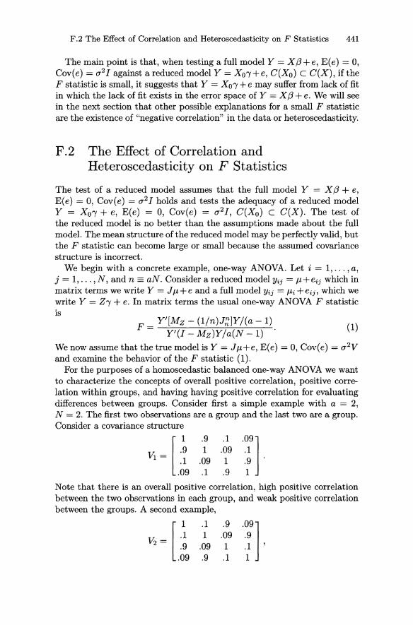
F.2 The Effect of Correlation and Heteroscedasticity on F Statistics 441
The main point is that, when testing a full model Y = X(3+e, E(e) = 0, Cov(e) = (J'2 J against a reduced model Y = Xo'Y+e, C(Xo) c C(X), if the F statistic is small, it suggests that Y = Xo'Y + e may suffer from lack of fit in which the lack of fit exists in the error space of Y = X(3 + e. We will see in the next section that other possible explanations for a small F statistic are the existence of "negative correlation" in the data or heteroscedasticity.
F.2 The Effect of Correlation and Heteroscedasticity on F Statistics
The test of a reduced model assumes that the full model Y = X(3 + e, E( e) = 0, Cov( e) = (J'2 J holds and tests the adequacy of a reduced model Y = Xo'Y + e, E(e) = 0, Cov(e) = (J'2J, C(Xo) c C(X). The test of the reduced model is no better than the assumptions made about the full model. The mean structure of the reduced model may be perfectly valid, but the F statistic can become large or small because the assumed covariance structure is incorrect.
We begin with a concrete example, one-way ANOVA. Let i = 1, ... , a, j = 1, ... , N, and n == aN. Consider a reduced model Yij = JL + eij which in matrix terms we write Y = J JL + e and a full model Yij = JLi + eij, which we write Y = Z'Y + e. In matrix terms the usual one-way ANOVA F statistic is
F = Y'[Mz - (1/n)J~JY/(a - 1) Y'(J - Mz)Y/a(N - 1) .
(1)
We now assume that the true model is Y = J JL+e, E(e) = 0, Cov(e) = (J'2y
and examine the behavior of the F statistic (1). For the purposes of a homoscedastic balanced one-way ANOVA we want
to characterize the concepts of overall positive correlation, positive correlation within groups, and having having positive correlation for evaluating differences between groups. Consider first a simple example with a = 2, N = 2. The first two observations are a group and the last two are a group. Consider a covariance structure
V:t= [ 1 .9 .1 .09] .9 1 .09 .1 .1 .09 1 .9 .
. 09 .1 .9 1
Note that there is an overall positive correlation, high positive correlation between the two observations in each group, and weak positive correlation between the groups. A second example,
Y2 = [ .~ .9 .09
.1 1
.09 .9
.9 .09 1 .1
.09] .9 .1 ' 1
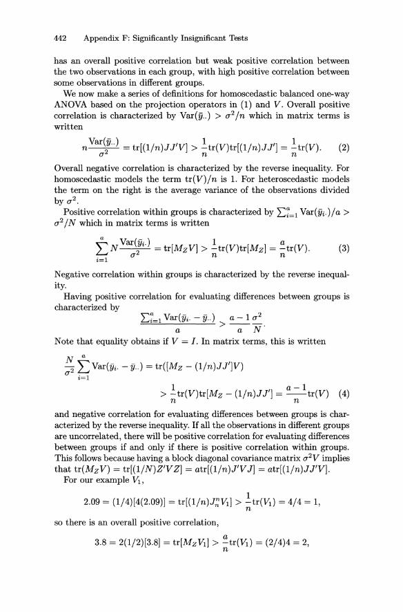
442 Appendix F: Significantly Insignificant Tests
has an overall positive correlation but weak positive correlation between the two observations in each group, with high positive correlation between some observations in different groups.
We now make a series of definitions for homoscedastic balanced one-way ANOVA based on the projection operators in (1) and V. Overall positive correlation is characterized by Var(y .. ) > a 2 /n which in matrix terms is written
n Var~ .. ) = tr[(l/n)JJ'V] > !:.tr(V)tr[(l/n)JJ'] = !:.tr(V). (2) ann
Overall negative correlation is characterized by the reverse inequality. For homoscedastic models the term tr(V)/n is 1. For heteroscedastic models the term on the right is the average variance of the observations divided bya2 •
Positive correlation within groups is characterized by E~=I Var(Yi.)/a > a2 / N which in matrix terms is written
~ Var(y·.} 1 a ~N 2 t = tr[MzV] > -tr(V)tr[Mz ] = -tr(V). ann
i=1
(3)
Negative correlation within groups is characterized by the reverse inequality.
Having positive correlation for evaluating differences between groups is characterized by
E~=I Var(Yi. - y .. ) a-I a 2 ==-"-----"=------':........:... > ---.
a a N Note that equality obtains if V = I. In matrix terms, this is written
N a
2" LVar(Yi. - y .. ) = tr([Mz - (l/n)JJ'lV) a i=1
1 a-I > -tr(V)tr[Mz - (l/n)JJ'] = -tr(V) (4)
n n
and negative correlation for evaluating differences between groups is characterized by the reverse inequality. If all the observations in different groups are uncorrelated, there will be positive correlation for evaluating differences between groups if and only if there is positive correlation within groups. This follows because having a block diagonal covariance matrix a 2V implies that tr(MzV) = tr[(l/N)Z'VZ] = atr[(l/n)J'V J] = atr[(l/n)JJ'V].
For our example VI,
1 2.09 = (1/4)[4(2.09)] = tr[(l/n)J~Vt] > -tr(Vt} = 4/4 = 1,
n
so there is an overall positive correlation,
a 3.8 = 2(1/2)[3.8] = tr[MzVI ] > -tr(VI ) = (2/4)4 = 2,
n
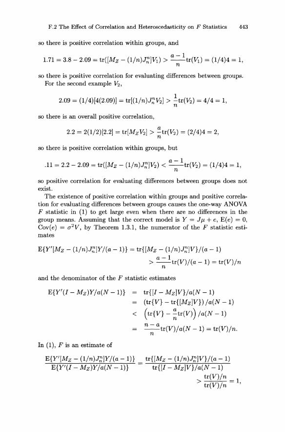
F.2 The Effect of Correlation and Heteroscedasticityon F Statistics 443
so there is positive correlation within groups, and
a-I 1.71 = 3.8 - 2.09 = tr([Mz - (l/n)J~lVl) > -tr(Vt} = (1/4)4 = 1,
n
so there is positive correlation for evaluating differences between groups. For the second example V:! ,
1 2.09 = (1/4)[4(2.09)] = tr[(I/n)J~V2] > -tr(V:!) = 4/4 = 1,
n
so there is an overall positive correlation,
a 2.2 = 2(1/2)[2.2] = tr[Mz V2] > -tr(V2 ) = (2/4)4 = 2,
n
so there is positive correlation within groups, but
a-I .11 = 2.2 - 2.09 = tr([Mz - (l/n)J~lV2) < --tr(V2 ) = (1/4)4 = 1,
n
so positive correlation for evaluating differences between groups does not exist.
The existence of positive correlation within groups and positive correlation for evaluating differences between groups causes the one-way ANOVA F statistic in (1) to get large even when there are no differences in the group means. Assuming that the correct model is Y = Jj.t + e, E(e) = 0, Cov(e) = a 2V, by Theorem 1.3.1, the numerator of the F statistic estimates
E{Y'[Mz - (l/n)J~]Y/(a -I)} = tr{[Mz - (l/n)J~lV}/(a - 1) a-I
> -tr(V)/(a - 1) = tr(V)/n n
and the denominator of the F statistic estimates
E{Y'(I - Mz)Y/a(N -I)} tr{[I - MzlV}/a(N - 1)
(tr{V} - tr{[MzlV}) /a(N - 1)
< (tr{V} - ~tr(V)) /a(N -1)
n-a --tr(V)/a(N -1) = tr(V)/n.
n
In (1), F is an estimate of
E{Y'[Mz - (l/n)J~]Y/(a - I)} tr{[Mz - (l/n)J~lV}/(a - 1) =~~~-7~~~~~~~
E{Y'(I - Mz)Y/a(N - I)} tr{[I - MzlV}/a(N -1)
tr(V)/n _ 1 > tr(V)/n - ,
444 Appendix F: Significantly Insignificant Tests
so having both positive correlation within groups and positive correlation for evaluating differences between groups tends to make F statistics large. Exactly analogous computations show that having both negative correlation within groups and negative correlation for evaluating differences between groups tends to make F statistics less than 1.
Another example elucidates some additional points. Suppose the observations have the correlation structure discussed in Subsection 13.3.1:
p 1 V3 = 2
[ 1 p
P P p3 p2
Using the same grouping structure as before, when 0 < p < 1, we have overall positive correlation because
1 + ~(3 + 2p + p2) = tr[(1/n)JJ'V31 > 1
and we have positive correlation within groups because
2(1 + p) = tr[MzV31 > 2.
If -1 < p < 0, the inequalities are reversed. Similarly, for -1 < p < 0 we have negative correlation for evaluating differences between groups because
1 + ~(1- 2p - p2)2 = tr([Mz - (1/n)JJ']V3) < 1.
However, we only get positive correlation for evaluating differences between groups when 0 < p < v'2 - 1. Thus, for negative p, we tend to get small F statistics, for 0 < p < v'2 - 1, we tend to get large F statistics, and for v'2 - 1 < p < 1, the result is not clear.
To illustrate, suppose p = 1 and the observations all have the same mean, then with probability 1, all the observations are equal and, in particular, fk = y .. with probability 1. It follows that
o = L:~-1 Var(Yi. - y .. ) < a-I a 2
a a N
and no positive correlation exists for evaluating differences between groups. More generally, for very strong positive correlations, both the numerator and the denominator of the F statistic estimate numbers that are close to o and both are smaller than they would be under V = I. On the other hand, it is not difficult to see that, for p = -1, the F statistic is O.
In the balanced heteroscedastic one-way ANOVA, V is diagonal. This generates equality between the left sides and right sides of (2), (3), and (4), so under heteroscedasticity F still estimates the number 1. We now
F.2 The Effect of Correlation and Heteroscedasticity on F Statistics 445
generalize the ideas of within group correlation and correlation for evaluating differences between groups, and see that heteroscedasticity can affect unbalanced one-way ANOVA.
In general, we test a full model Y = X/3+e, E(e) = 0, Cov(e) = a2[
against a reduced model Y = Xol' + e, in which C(Xo) C C(X). We examine the F statistic when the true model is Y = Xol' + e, E(e) = 0, Cov(e) = a 2V. Using arguments similar to those for balanced one-way ANOVA, having
1 r(X) tr[MV] > -tr(V)tr[M] = -tr(V)
n n
and
tr([M - MoW) > ~tr(V)tr[M - Mo] = r(X) - r(Xo) tr(V) n n
causes large F statistics even when the mean structure of the reduced model is true, and reversing the inequalities causes small F statistics. These are merely sufficient conditions to have the tests intuitively behave certain ways. The actual behavior of the tests under normal distributions can be determined numerically, cf. Christensen and Bedrick (1997).
These covariance conditions can be caused by patterns of positive and negative correlations as discussed earlier, but they can also be caused by heteroscedasticity. For example, consider the behavior of the unbalanced one-way ANOVA F test when the observations are uncorrelated but heteroscedastic. For concreteness, assume that Var(Yij) = a'f. Because the observations are uncorrelated, we need only check the condition
1 a tr[MV] == tr[MzV] > -tr(V)tr[Mz ] = -tr(V),
n n
which amounts to a a N "2/ "i 2 L..J ai a > L..J -ai . i=l i=l n
Thus, when the groups means are equal, F statistics will get large if many observations are taken in groups with small variances and few observations are taken on groups with large variances. F statistics will get small if the reverse relationship holds.
The general condition
1 r(X) tr[MV] > -tr(V)tr[M] = -tr(V)
n n
is equivalent to

446 Appendix F: Significantly Insignificant Tests
So, under homoscedasticity, positive correlation in the full model amounts to having an average variance for the predicted values (averaging over the rank of the covariance matrix of the predicted values) that is larger than the common variance of the observations. Negative correlation in the full model involves reversing the inequality. Similarly, having positive correlation for distinguishing the full model from the reduced model means
Z=~=1 Var(x~,B - x~ii') = tr[(M - Mo)V] > tr(V) = Z=~=1 Var(Yi) r(X) - r(Xo) r(M - Mo) n n·
Appendix G: Randomization Theory Models
The division of labor in statistics has traditionally designated randomization theory as an area of nonparametric statistics. Randomization theory is also of special interest in the theory of experimental design because randomization is used to justify the analysis of designed experiments.
It can be argued that the linear models given in Chapter 8 are merely good approximations to more appropriate models based on randomization theory. One aspect of this argument is that the F tests based on the theory of normal errors are a good approximation to randomization (permutation) tests. Investigating this is beyond the scope of a linear models book, cf. Hinkelmann and Kempthorne (1994) and Puri and Sen (1971). Another aspect of the approximation argument is that the BLUEs under randomization theory are precisely the least squares estimates. By Theorem 10.4.5, to establish this we need to show that C(V X) c C(X) for the model
y = X.B + e, E(e) = 0, Cov(e) = V,
where V is the covariance matrix under randomization theory. This argument will be examined here for two experimental design models: the model for a completely randomized design and the model for a randomized complete block design. First, we introduce the subject with a discussion of simple random sampling.
448 Appendix G: Randomization Theory Models
G.1 Simple Random Sampling
Randomization theory for a simple random sample assumes that observations Yi are picked at random (without replacement) from a larger finite population. Suppose the elements of the population are S1, S2, ... , S N.
We can define elementary sampling random variables for i = 1, ... , n and j= 1, ... ,N
O~ = {I if Yi = Sj J 0 otherwise .
Under simple random sampling without replacement
. . 1 E(oj) = Pr(oj = 1) = N'
•• 1 • • 1 {liN if (i,j) = (if,j') E(ojo}) = Pr(ojo} = 1) = 1IN(N - 1) if i =f if and j =f jf
o otherwise
If we write J.L = Ef=1 sjlN and 0-2 = Ef=1 (Sj - J.L)2 IN, then
N N
Yi = LO}Sj = J.L+ LO}(Sj - J.L). j=1 j=1
Letting ei = Ef=1 o;(Sj - J.L) gives the linear model
The population mean J.L is a fixed unknown constant. The eiS have the properties
N N
Var(ei) = E[e~J = L L (Sj - J.L)(Sjl - J.L)E[o}O}/J j=1 j'=1
N
L(Sj - J.Lf IN = 0-2. j=1
For i =f if
N N
E[eied = L L(Sj - J.L)(Sj' - J.L)E[o}ofJ j=1 j'=1
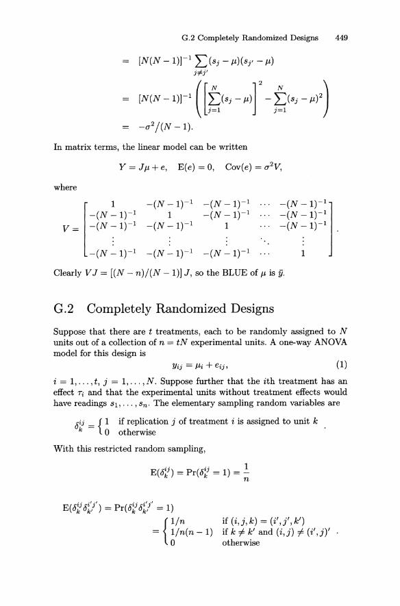
G.2 Completely Randomized Designs 449
#j'
[N(N - 1 W' ([t,(.; -~) r -t,(.; -~),) = -u2 /(N -1).
In matrix terms, the linear model can be written
where
-(N _1)-1 1 -(N - 1)-1 . . . -(N - 1)-1 [
1
V = -(N ~ 1)-1 -(N - 1)-1 1 . . . -(N - 1)-1 .
-(N -1)-1 -(N - 1)-1 ... -(N _1)_11
· '. . · ... · . . . -(N _1)-1 -(N - 1)-1 -(N - 1)-1 . . . 1
Clearly V J = [(N - n)/(N - 1)] J, so the BLUE of /-L is y.
G.2 Completely Randomized Designs
Suppose that there are t treatments, each to be randomly assigned to N units out of a collection of n = tN experimental units. A one-way ANOVA model for this design is
Yij = /-Li + eij, (1)
i = 1, ... , t, j = 1, ... , N. Suppose further that the ith treatment has an effect Ti and that the experimental units without treatment effects would have readings 81. ... , 8 n . The elementary sampling random variables are
8ij = {1 if replication j of treatment i is assigned to unit k k 0 otherwise
With this restricted random sampling,
E(8~8t/) = Pr(8~8t/ = 1)
{lin
= ~/n(n -1) 'f (. . k) ("" k') 1 Z,J, = Z ,J , if k =j:. k' and (i,j) =j:. (i',j)' otherwise
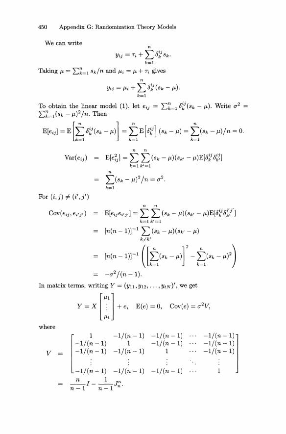
450 Appendix G: Randomization Theory Models
We can write n
_ "'" ~ij Yij - 'Ti + L..J uk Sk· k=l
Taking f-L = L:~=1 skin and f-Li = f-L + 'Ti gives n
Yij = f-Li + L8~(Sk - f-L). k=l
To obtain the linear model (1), let eij = L:~=1 8~ (Sk - f-L). Write (72 = L:~=1 (Sk - f-L)2/n. Then
E[eij] = E[t8~(Sk - f-L)] = tE[8~] (Sk - f-L) = t(Sk - f-L)/n = O. k=l k=l k=l
n n
Var(eij) = E[e~j] = L L (Sk - f-L)(Sk' - f-L)E[8~ 8~] k=l k'=l
n
L(Sk - f-L)2/n = (72. k=l
For (i,j) =I- (i',j') n n
Cov(eij, ei'j') = E[eijei'j'] = L L (Sk - f-L)(Sk' - f-L)E[8~8t/] k=l k'=l
k#k'
~ [n(n -1)]-' ([t,(Sk -p)r -t,(Sk -P)') -(72/(n - 1).
In matrix terms, writing Y = (Yll, Y12, ... ,YtN)', we get
y ~ X [:l + e, E(e) ~ 0, COYle) ~ q'V,
where
[ -1/(! -1) -l/(n -1) -l/(n - 1) -l/(n -1)
1 -l/(n - 1) -l/(n -1)
V = -l/(n - 1) -l/(n - 1) 1 -l/(n -1)
-l/(n - 1) -l/(n - 1) -l/(n -1) 1
nIl r n-1 - n-1 n'

G.3 Randomized Complete Block Designs 451
It follows that
VX = _n_X _ _ I_J;:x. n-I n-I
Since J E C(X), C(VX) C C(X), and least squares estimates are BLUEs. Standard errors for estimable functions can be found as in Section 11.1 using the fact that this model involves only one cluster.
Exercise G.1 Establish whether least squares estimates are BLUEs in a completely randomized design with unequal numbers of observations on the treatments.
G.3 Randomized Complete Block Designs
Suppose there are a treatments and b blocks. The experimental units must be grouped into b blocks, each of a units. Let the experimental unit effects be Skj, k = 1, ... , a, j = 1, ... , b. Treatments are assigned at random to the a units in each block. The elementary sampling random variables are
i {I if treatment i is assigned to unit k in block j 8kJo = 0 otherwise
001 E(8ko ) = Pr(8ko = 1) =-.
J J a
{ila if (i,j,k) = (i',j',k')
i i ' _ i i ' _ _ IIa2 if j i- j' E(8kikljl) - Pr(8kj 8kljl - 1) - I ( )·f· ., k.../.. k' O"'/" 0' 1 aa-I 1 J=J, I ,Z,Z
o otherwise
If Qi is the additive effect of the ith treatment and {3j == s.j, then
a
Yij = Qi + {3j + 2: 8L(Skj - (3j). k=l
Letting eij = :E~=l 8~j (Skj - (3j) gives the linear model
(1)
The column space of the design matrix for this model is precisely that of the model considered in Section 8.3. Let O'J = :E~=l (Skj - {3j)2 la. Then
a
E[eij] = 2:(Skj - {3j)/a = 0 k=l

452 Appendix G: Randomization Theory Models
For j =/:- j'
Forj=j',i=/:-i'
a a
L L (Skj - {3j)(Sk1j - {3j)E[c5~jc5~'j] k=1 k'=1
a
= L(Skj - {3j)2/a = aJ. k=1
a a
L L (Skj - {3j)(Sk 1 jl - {3i' )E[c5L c5k1i'] k=1 k'=1
a a
a-2 L(skj -(3j) L(Skljl -(3i') k=1 k'=1
o.
a a
L L (Skj - {3j)(Sk1 j - {3j)E[c5~jc5klj] k=1 k'=1
k#k'
~ laCa -l)r' ([t,C',j -/lj)]' - t,CSk! -/lj)') -aJ!(a -1).
Before proceeding, we show that although the terms {3j are not known, the differences among these are known constants under randomization theory. For any unit k in block j, some treatment is assigned, so E~=1 c5~j = 1.
a
a. + {3j + L(Skj - (3j) k=1
Therefore, Y-j - y.jl = {3j - {3i' = s.j - s-j'. Since these differences are fixed and known, there is no basis for a test of Ho : {31 = ... = {3b. In fact, the linear model is not just model (1) but model (1) subject to these estimable constraints on the f3s.

G.3 Randomized Complete Block Designs 453
To get best linear unbiased estimates we need to assume that (J'~ = (J'~ = . .. = (J'~ = (J'2. We can now write the linear model in matrix form and establish that least squares estimates of treatment means and contrasts in the O!iS are BLUEs. In the discussion that follows, we use notation from Section 7.1. Model (1) can be rewritten
Y = X7] + e, E(e) = 0, Cov(e) = V, (2)
where 7] = [j.t,O!l'''',O!a,,lh, ... ,,8b]'. If we let X 2 be the columns of X corresponding to ,81, ... , ,8b, then (cf. Section 11.1)
v = (J'2 [aj(a - 1)] [1 - (lja)X2X~]
= (J'2 [aj(a - 1)] [1 - Mp. - M,e].
If model (2) were the appropriate model, checking that C(V X) c C(X) would be trivial based on the fact that C(X2) C C(X). However, we must account for the estimable constraints on the model discussed above. In particular, consider
where tij = ,8j - fJ. = y.j - y .. = s-j - S ...
This is a fixed known quantity. Proceeding as in Section 3.3, the model is subject to the estimable constraint
Normally a constraint has the form A',8 = d, where d is known. Here d = M,eY, which appears to be random but, as discussed, M,eY is not random; it is fixed and upon observing Y it is known.
The equivalent reduced model involves Xo = (I -MMP)X = (1 -M,e)X and a known vector Xb = M,eY. Thus the constrained model is equivalent to
(Y - M,eY) = (I - M,e)X"'( + e. (3)
We want to show that least squares estimates of contrasts in the O!S
based on Y are BLUEs with respect to this model. First we show that least squares estimates from model (3) based on (Y - M,eY) = (1 - M,e)Y are BLUEs. We need to show that
C(V(1 - M,e)X) = C[(I - MJ1. - M,e)(1 - M,e)X] c C[(I - M,e)X].
Because (1 - Mp. - M,e)(I - M,e) = (1 - Mp. - M,e), we have
C(V(1 - M,e)X) = C[(1 - Mp. - M,e)X];
and because C(I - Mp. - M,e) C C(1 - M,e) we have
C[(1 - Mp. - M,e)X] C C[(1 - M,e)X].
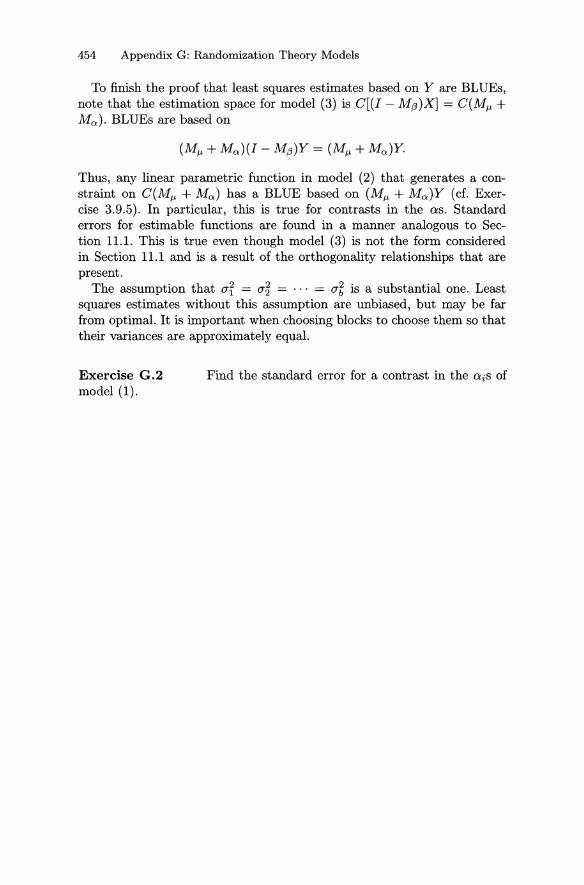
454 Appendix G: Randomization Theory Models
To finish the proof that least squares estimates based on Y are BLUEs, note that the estimation space for model (3) is C[(J - M(3)X] = C(Mp. + Mo.). BLUEs are based on
Thus, any linear parametric function in model (2) that generates a constraint on C(Mp. + Mo.) has a BLUE based on (M,." + Mo.)Y (cf. Exercise 3.9.5). In particular, this is true for contrasts in the as. Standard errors for estimable functions are found in a manner analogous to Section 11.1. This is true even though model (3) is not the form considered in Section 11.1 and is a result of the orthogonality relationships that are present.
The assumption that ar = a~ = ... = a~ is a substantial one. Least squares estimates without this assumption are unbiased, but may be far from optimal. It is important when choosing blocks to choose them so that their variances are approximately equal.
Exercise G.2 model (1).
Find the standard error for a contrast in the aiS of
References
Aitchison, J. and Dunsmore, I. R (1975). Statistical Prediction Analysis. Cambridge University Press, Cambridge.
Anderson, T. W. (1984). An Introduction to Multivariate Statistical Analysis, Second Edition. John Wiley and Sons, New York.
Andrews, D. F. (1974). A robust method for multiple regression. Technometrics, 16, 523-531.
Arnold, S. F. (1981). The Theory of Linear Models and Multivariate Analysis. John Wiley and Sons, New York.
Atkinson, A. C. (1981). Two graphical displays for outlying and influential observations in regression. Biometrika, 68, 13-20.
Atkinson, A. C. (1982). Regression diagnostics, transformations and constructed variables (with discussion). Journal of the Royal Statistical Society, Series B, 44, 1-36.
Atkinson, A. C. (1985). Plots, Transformations, and Regression: An Introduction to Graphical Methods of Diagnostic Regression Analysis. Oxford University Press, Oxford.
Atwood, C. L. and Ryan, T. A., Jr. (1977). A class of tests for lack of fit to a regression model. Unpublished manuscript.
Bailey, D. W. (1953). The Inheritance of Maternal Influences on the Growth of the Rat. Ph.D. Thesis, University of California.
Bedrick, E. J., Christensen, R, and Johnson, W. (1996). A new perspective on priors for generalized linear models. Journal of the American Statistical Association, 91, 1450-1460.
456 References
Belsley, D. A. (1991). Collinearity Diagnostics: Collinearity and Weak Data in Regression. John Wiley and Sons, New York.
Belsley, D. A., Kuh, E., and Welsch, R. E. (1980). Regression Diagnostics: Identifying Influential Data and Sources of Collinearity. John Wiley and Sons, New York.
Benedetti, J. K. and Brown, M. B. (1978). Strategies for the selection of log-linear models. Biometrics, 34, 680-686.
Berger, J. O. (1985). Statistical Decision Theory and Bayesian Analysis. SpringerVerlag, New York.
Blom, G. (1958). Statistical Estimates and Transformed Beta Variates. John Wiley and Sons, New York.
Box, G. E. P. and Cox, D. R. (1964). An analysis of transformations. Journal of the Royal Statistical Society, Series B, 26, 211-246.
Box, G. E. P. and Draper, N. R. (1987). Empirical Model-Building and Response Surfaces. John Wiley and Sons, New York.
Box, G. E. P., Hunter, W. G., and Hunter, J. S. (1978). Statistics for Experimenters. John Wiley and Sons, New York.
Box, G. E. P. and Tiao, G. C. (1973). Bayesian Inference in Statistical Analysis. John Wiley and Sons, New York.
Brockwell, P. J. and Davis, R. A. (1991). Time Series: Theory and Methods, Second Edition. Springer-Verlag, New York.
Brownlee, K. A. (1965). Statistical Theory and Methodology in Science and Engineering, Second Edition. John Wiley and Sons, New York.
Christensen, R. (1984). A note on ordinary least squares methods for two-stage sampling. Journal of the American Statistical Association, 79, 720-72l.
Christensen, R. (1987a). Plane Answers to Complex Questions: The Theory of Linear Models. Springer-Verlag, New York.
Christensen, R. (1987b). The analysis of two-stage sampling data by ordinary least squares. Journal of the American Statistical Association, 82, 492-498.
Christensen, R. (1989). Lack of fit tests based on near or exact replicates. Annals of Statistics, 17, 673-683.
Christensen, R. (1991). Small sample characterizations of near replicate lack of fit tests. Journal of the American Statistical Association, 86, 752-756.
Christensen, R. (1993). Quadratic covariance estimation and equivalence of predictions. Mathematical Geology, 25, 541-558.
Christensen, R. (1995). Comment on Inman (1994). The American Statistician, 49,400.
Christensen, R. (1996a). Analysis of Variance, Design, and Regression: Applied Statistical Methods. Chapman and Hall, London.
References 457
Christensen, R {1996b}. Exact tests for variance components. Biometrics, 52, 309-315.
Christensen, R {1997}. Log-Linear Models and Logistic Regression, Second Edition. Springer-Verlag, New York.
Christensen, R {2001}. Advanced Linear Modeling: Multivariate, Time Series, and Spatial Data; Nonpammetric Regression, and Response Surface Maximization, Second Edition. Springer-Verlag, New York.
Christensen, R {2001}. Estimability of identifiability? Unpublished Manuscript.
Christensen, R and Bedrick, E. J. {1997}. Testing the independence assumption in linear models. Journal of the American Statistical Association, 92, 1006-1016.
Christensen, Rand Bedrick, E. J. {1999}. A survey of some new alternatives to Wald's variance component test. Tatm Mountains Mathematical Publications, 17, 91-102.
Christensen, R, Johnson, W., and Pearson, L. M. {1992}. Prediction diagnostics for spatial linear models. Biometrika, 79, 583-59l.
Christensen, R, Johnson, W., and Pearson, L. M. {1993}. Covariance function diagnostics for spatial linear models. Mathematical Geology, 25, 145-160.
Christensen, R, Pearson, L. M., and Johnson, W. {1992}. "Case deletion diagnostics for mixed models." Technometrics, 34, 38-45.
Cochran, W. G. and Cox, G. M. {1957}. Experimental Designs, Second Edition. John Wiley and Sons, New York.
Cook, R. D. {1977}. Detection of influential observations in linear regression. Technometrics, 19, 15-18.
Cook, R D. and Weisberg, S. {1982}. Residuals and Influence in Regression. Chapman and Hall, New York.
Cook, R D. and Weisberg, S. {1994}. An Introduction to Regression Gmphics. John Wiley and Sons, New York.
Cornell, J. A. {1988}. Analyzing mixture experiments containing process variables. A split plot approach. Journal of Quality Technology, 20, 2-23.
Cox, D. R {1958}. Planning of Experiments. John Wiley and Sons, New York.
Cox, D. R and Hinkley, D. V. {1974}. Theoretical Statistics. Chapman and Hall, London.
Cressie, N. {1993}. Statistics for Spatial Data, Revised Edition. John Wiley and Sons, New York.
Daniel, C. {1959}. Use of half-normal plots in interpreting factorial two-level experiments. Technometrics, 1, 311-34l.
Daniel, C. {1976}. Applications of Statistics to Industrial Experimentation. John Wiley and Sons, New York.

458 References
Daniel, C. and Wood, F. S. (1980). Fitting Equations to Data, Second Edition. John Wiley and Sons, New York.
Davies, R. B. (1980). The distribution of linear combinations of X2 random variables. Applied Statistics, 29, 323-333.
de Finetti, B. (1974, 1975). Theory of Probability, Vols. 1 and 2. John Wiley and Sons, New York.
DeGroot, M. H. (1970). Optimal Statistical Decisions. McGraw-Hill, New York.
Doob, J. L. (1953). Stochastic Processes. John Wiley and Sons, New York.
Draper, N. and Smith, H. (1981). Applied Regression Analysis, Second Edition. John Wiley and Sons, New York.
Duan, N. (1981). Consistency of residual distribution functions. Working Draft No. 80l-1-HHS (106B-800l0), Rand Corporation, Santa Monica, CA.
Durban, J. and Watson, G. S. (1951). Testing for serial correlation in least squares regression II. Biometrika, 38, 159-179.
Eaton, M. L. (1983). Multivariate Statistics: A Vector Space Approach. John Wiley and Sons, New York.
Eaton, M. L. (1985). The Gauss-Markov theorem in multivariate analysis. In Multivariate Analysis - VI, edited by P. R. Krishnaiah. Elsevier Science Publishers B. V.
Ferguson, T. S. (1967). Mathematical Statistics: A Decision Theoretic Approach. Academic Press, New York.
Fienberg, S. E. (1980). The Analysis of Cross-Classified Categorical Data, Second Edition. MIT Press, Cambridge, MA.
Fisher, R. A. (1935). The Design of Experiments, Ninth Edition, 1971. Hafner Press, New York.
Furnival, G. M. and Wilson, R. W. (1974). Regression by leaps and bounds. Technometrics, 16, 499-511.
Geisser, S. (1971). The inferential use of predictive distributions. In Foundations of Statistical Inference, edited by V.P. Godambe and D.A. Sprott. Holt, Reinhart, and Winston, Toronto.
Geisser, S. (1993). Predictive Inference. An Introduction. Chapman and Hall, New York.
Gnanadesikan, R. (1977). Methods for Statistical Analysis of Multivariate Observations. John Wiley and Sons, New York.
Goldstein, M. and Smith, A. F. M. (1974). Ridge-type estimators for regression analysis. Journal of the Royal Statistical Society, Series B, 26, 284-291.
Graybill, F. A. (1976). Theory and Application of the Linear Model. Duxbury Press, North Scituate, MA.

References 459
Grizzle, J. E., Starmer, C. F., and Koch, G. G. (1969). Analysis of categorical data by linear models. Biometrics, 25, 489-504.
Guttman, 1. (1970). Statistical Tolerance Regions. Hafner Press, New York.
Haberman, S. J. (1974). The Analysis of Frequency Data. University of Chicago Press, Chicago.
Hartigan, J. (1969). Linear Bayesian methods. Journal of the Royal Statistical Society, Series B, 31, 446-454.
Harville, D. A. (1985). Decomposition of prediction error. Journal of the American Statistical Association, 80, 132-138.
Haslett, J. and Hayes, K. (1998). Residuals for the linear model with general covariance structure. Journal of the Royal Statistical Society, Series B, 60, 201-215.
Henderson, C. R. (1953). Estimation of variance and covariance components. Biometrics, 9, 226-252.
Hinkelmann, K. and Kempthorne, O. (1994). Design and Analysis of Experiments. John Wiley and Sons, New York.
Hinkley, D. V. (1969). Inference about the intersection in two-phase regression. Biometrika, 56, 495-504.
Hochberg, Y. and Tamhane, A. (1987). Multiple Comparison Procedures. John Wiley and Sons, New York.
Hoerl, A. E. and Kennard, R. (1970). Ridge regression: biased estimation for non-orthogonal problems. Technometrics, 12, 55-67.
Hsu, J. C. (1996). Multiple Comparisons: Theory and Methods. Chapman and Hall, London.
Jeffreys, H. (1961). Theory of Probability, Third Edition. Oxford University Press, London.
Johnson, R. A. and Wichern, D. W. (1988). Applied Multivariate Statistical Analysis. Prentice-Hall, Englewood Cliffs, NJ.
Khuri, A. 1., Mathew, T., and Sinha, B. K. (1998). Statistical Tests for Mixed Linear Models. John Wiley and Sons, New York.
Lehmann, E. L. (1983) Theory of Point Estimation. John Wiley and Sons, New York.
Lehmann, E. L. (1986) Testing Statistical Hypotheses, Second Edition. John Wiley and Sons, New York.
Lin, T-H. and Harville, D. A. (1991). Some alternatives to Wald's confidence interval and test. Journal of the American Statistical Association 86, 179-187.
Lindley, D. V. (1971). Bayesian Statistics: A Review. SIAM, Philadelphia.

460 References
McCullagh, P. (2000). Invariance and factorial models, with discussion. Journal of the Royal Statistical Society, Series B, 62, 209-238.
McCullagh, P. and NeIder, J.A. (1989). Generalized Linear Models, Second Edition. London: Chapman and Hall.
Mandansky, A. (1988), Prescriptions for Working Statisticians. Springer-Verlag, New York.
Marquardt, D. W. (1970). Generalized inverses, ridge regression, biased linear estimation, and nonlinear estimation. Technometrics, 12, 591-612.
Martin, R J. (1992). Leverage, influence and residuals in regression models when observations are correlated. Communications in Statistics - Theory and Methods, 21, 5, 1183-1212.
Mathew, T. and Sinha, B. K. (1992). Exact and optimum tests in unbalanced split-plot designs under mixed and random models. Journal of the American Statistical Association, 87, 192-200
Miller, R G., Jr. (1981). Simultaneous Statistical Inference, Second Edition. Springer-Verlag, New York.
Miller, F. R, Neill, J. W., and Sherfey, B. W. (1998) Maximin clusters for near replicate regression lack of fit tests. Annals of Statistics, 26, 1411-1433.
Miller, F. R, Neill, J. W., and Sherfey, B. W. (1999) Implementation of maximin power clustering criterion to select near replicates for regression lack-of-fit tests. Journal of the American Statistical Association, 94, 610-620.
Monlezun, C. J. and Blouin, D. C. (1988). A general nested split-plot analysis of covariance. Journal of the American Statistical Association, 83, 818-823.
Morrison, D. F. (1976). Multivariate Statistical Methods. McGraw-Hill, New York.
Mosteller, F. and Tukey, J. W. (1977). Data Analysis and Regression. AddisonWesley, Reading, MA.
Neill, J. W. and Johnson, D. E. (1984). Testing for lack of fit in regression - A review. Communications in Statistics, Part A - Theory and Methods, 13, 485-511.
Neter, J., Wasserman, W., and Kutner, M. H. (1985). Applied Linear Statistical Models. Richard D. Irwin Inc., Homewood, FL.
Ofversten, J. (1993). Exact Tests for Variance Components in Unbalanced Linear Models. Biometrics, 49, 45-57.
Peixoto, J. 1. (1993). Four equivalent definitions of reparameterizations and restrictions in linear models. Communications in Statistics, A, 22, 283-299.
Picard, R R and Berk, K. N. (1990). Data splitting. The American Statistician, 44, 140-147.
Picard, R R and Cook, R D. (1984). Cross-validation of regression models. Journal of the American Statistical Association, 79, 575-583.
References 461
Puri, M. L. and Sen, P. K. (1971). Nonparametric Methods in Multivariate Analysis. John Wiley and Sons, New York.
Raiffa, H. and Schlaifer, R. (1961). Applied Statistical Decision Theory. Division of Research, Graduate School of Business Administration, Harvard University, Boston.
Rao, C. R. (1971). Estimation of variance and covariance components-MINQUE theory. Journal of Multivariate Analysis, 1, 257-275.
Rao, C. R. (1973). Linear Statistical Inference and Its Applications, Second Edition. John Wiley and Sons, New York.
Ripley, B. D. (1981). Spatial Statistics. John Wiley and Sons, New York.
Savage, L. J. (1954). The Foundations of Statistics. John Wiley and Sons, New York.
Schafer, D. W. (1987). Measurement error diagnostics and the sex discrimination problem. Journal of Business and Economic Statistics, 5, 529-537.
Schatzoff, M., Tsao, R., and Fienberg, S. (1968). Efficient calculations of all possible regressions. Technometrics, 10, 768-779.
Scheffe, H. (1959). The Analysis of Variance. John Wiley and Sons, New York.
Searle, S. R. (1971), Linear Models. John Wiley and Sons, New York.
Searle, S. R., Casella, G., and McCulloch, C. (1992), Variance Components. John Wiley and Sons, New York.
Searle, S. R. and Pukelsheim, F. (1987). Estimation of the mean vector in linear models, Technical Report BU-912-M, Biometrics Unit, Cornell University, Ithaca, NY.
Seber, G. A. F. (1966). The Linear Hypothesis; A General Theory. Griffin, London.
Seber, G. A. F. (1977). Linear Regression Analysis. John Wiley and Sons, New York.
Seely, J. F. and EI-Bassiouni, Y. (1983). Applying Wald's variance component test. Annals of Statistics, 11, 197-201.
Shapiro, S. S. and Francia, R. S. (1972). An approximate analysis of variance test for normality. Journal of the American Statistical Association, 67, 215-216.
Shapiro, S. S. and Wilk, M. B. (1965). An analysis of variance test for normality (complete samples). Biometrika, 52, 591-611.
Shewhart, W. A. (1931). Economic Control of Quality. Van Nostrand, New York.
Shewhart, W. A. (1939). Statistical Method from the Viewpoint of Quality Control. Graduate School of the Department of Agriculture, Washington. Reprint (1986), Dover, New York.
Shillington, E. R. (1979). Testing Lack of Fit in Regression Without Replication. Canadian Journal of Statistics, 7, 137-146.

462 References
Shumway, R. H. and Stoffer, D. S. (2000). Times Series Analysis and Its Applications. Springer-Verlag, New York.
Skinner, C. J., Holt, D., and Smith, T. M. F. (1989). Analysis of Complex Surveys. John Wiley and Sons, New York.
Smith, A. F. M. (1986). Comment on an article by B. Efron. The American Statistician, 40, 10.
Snedecor, G. W. and Cochran, W. G. (1980). Statistical Methods, Seventh Edition. Iowa State University Press, Ames.
Sulzberger, P. H. (1953). The effects of temperature on the strength of wood, plywood and glued joints. Department of Supply, Report ACA-46, Aeronautical Research Consultative Committee, Australia.
Utts, J. (1982). The rainbow test for lack of fit in regression. Communications in Statistics-Theory and Methods, 11, 2801-2815.
Weisberg, S. (1985). Applied Linear Regression, Second Edition. John Wiley and Sons, New York
Wermuth, N. (1976). Model search among multiplicative models. Biometrics, 32, 253-264.
Williams, E. J. (1959). Regression Analysis. John Wiley and Sons, New York.
Zellner, A. (1971) An Introduction to Bayesian Inference in Econometrics. John Wiley and Sons, New York.

Author Index
Aitchison, J., 48, 153 Anderson, T. W., 132 Andrews, D. F., 368 Arnold, S. F., 18, 334 Atkinson, A. C., 322, 340, 342, 366 Atwood, C. L., 147
Bailey, D. W., 182 Bedrick, E. J., 40, 308, 341, 342, 445 Belsley, D. A., 381 Benedetti, J. K., 193 Berger, J. 0., 39 Berk, K. N., 362 Blom, G., 334 Blouin, D. C., 255 Box, G. E. P., 39, 153, 155, 366 Brockwell, P. J., 132 Brown, M. B., 193 Brownlee, K. A., 368
Casella, G., 279, 289, 295 Christensen, R., ix, 13, 19, 40, 75, 107,
114, 130, 131, 132, 143, 144, 145, 151, 186, 189, 193, 197, 207, 255, 280, 284, 295, 304, 308, 320, 337, 341, 342, 362, 367, 368, 386, 434, 437, 440, 445
Cochran, W.G., 114, 151, 197,209,227 Cook, R. D., xii, 322, 362, 364, 365, 366,
367 Cornell, J. A., 276 Cox, D. R., 31, 197, 209, 366 Cox, G. M., 197, 227 Cressie, N., 132
Daniel, C., 123, 341, 368 Davies, R. B., 307, 425 Davis, R. A., 132 de Finetti, B., 39 DeGroot, M. H., 39, 44 Doob, J. L., 132 Draper, N., 123, 127, 154, 322, 368 Duan, N., 334 Dunsmore, I. R., 48, 153 Durbin, J., 343
Eaton, M. L., xi, 19, 280 EI-Bassiouni, Y., 302
Ferguson, T. S., 236 Fienberg, S. E., 186, 189, 370 Fisher, R. A., 197, 272 Francia, R. S., 337 Furnival, G. M., 370

464 Author Index
Geisser, S., 39, 48, 131 Gnanadesikan, R., 143 Goldstein, M., 389 Graybill, F. A., 19 Grizzle, J. E., 366, 367 Guttman, I., 48
Haberman, S. J., xii Hartigan, J., 131 Harville, D. A., 280, 306 Haslett, J., 362 Hayes, K., 362 Henderson, C. R., 298 Hinkelmann, K., 197, 447 Hinkley, D. V., 31, 154 Hochberg, Y., 107 Hoerl, A. E., 387 Holt, D., 255 Hsu, J. C., 107 Hunter, J. S., 153 Hunter, W. G., 153
Jeffreys, H., 39 Johnson, D. E., 143 Johnson, R. A., 386 Johnson, W., 40, 41, 362
Kempthorne, 0., 197, 447 Kennard, R., 387 Khuri, A. I., 279 Koch, G. G., 366, 367 Kuh, E., 381 Kutner, M. H., 114
Lehmann, E. L., 30, 31, 428 Lin, T-H., 306 Lindley, D. V., 39
McCullagh, P., 13, 205 McCulloch, C., 279, 289, 295 Mandansky, A., 355 Marquardt, D. W., 386 Martin, R. J., 362 Mathew, T., 255, 279 Miller, F. R., 143 Miller, R. G., Jr., 107 Monlezun, C. J., 255 Morrison, D. F., 134 Mosteller, F., 389
Neill, J. W., 143 NeIder, J. A., 13 Neter, J., 114
Ofversten, J., 304
Pearson, L. M., 362 Peixoto, J. L., 53 Picard, R. R., 362 Pukelsheim, F., 235 Puri, M. L., 447
Raiffa, H., 39 Rao, C. R., 19,297,367,424 Ripley, B. D., 132 Ryan, T. A., Jr., 147
Savage, L. J., 39 Schafer, D. W., 42 Schlaifer, R., 39 Schatzoff, M., 370 Scheffe, H., 19, 182, 188 Searle, S. R., 19, 235, 279, 289, 295, 298 Seber, G. A. F., 19 Seely, J. F., 302 Sen, P. K., 447 Shapiro, S. S., 337 Sherfey, B. W, 143 Shewhart, W. A., 341 Shillington, E. R., 143 Shumway, R. H., 132 Sinha, B. K., 255, 279 Skinner, C. J., 255 Smith, A. F. M., 131,389 Smith, H., 123, 127, 322, 368 Smith, T. M. F., 255 Snedecor, G. W., 114, 151, 209 Starmer, C. F., 366, 367 Stoffer, D. S., 132 Sulzberger, P. H., 228
Tamhane, A., 107 Tiao, G. C., 39 Tsao, R., 370 Thkey, J. W., 389
Utts, J., 147, 365
Wasserman, W., 114

Watson, G. S., 343 Weisberg, S., xii, 123,322,364,366,367 Welsch, R. K, 381 Wermuth, N., 193 Wichern, D. W., 386 Wilk, M. B., 337
Author Index 465
Williams, K J., 288 Wilson, R. W., 370 Wood, F. S., 123, 368
Zellner, A., 39

Subject Index
0: level, see tests of hypotheses ACOVA, see analysis of covariance, ACOVA table, 215 added variable plot, 215, 355, 357 adjusted R2, 371 adjusted treatment means, 224 alternating additive effects, 206 analysis of covariance, 209
for BIBs, 219 estimation, 211 missing observations, 216 testing, 213
analysis of variance, BIBs, 219, 309 one-way, 91 multiway, 156 three-factor
balanced, 186 unbalanced, 188
two-factor balanced with interaction, 163 balanced without interaction, 156 proportional numbers, 176 unbalanced, 177
ANOVA, see analysis of variance
ANOVA table, 99, 126, 161, 171 assumptions, 320, 437
backwards elimination, 375 balanced ANOVA, see analysis of vari
ance balanced incomplete block designs, 219,
309 balanced two-way ANOVA, 156, 163 Bayesian statistics, 39, 131, 287 basis, 393 best linear unbiased estimate, 28, 34,
37, 231, 250, 256, 260 best linear predictor, 130, 281 best linear unbiased predictor, 135, 281,
322 best predictor, 132, 135, 281 best subset selection, 370 BIB, see balanced incomplete block de-
signs binomial distribution, 367 blocking, 196 BLUE, see best linear unbiased esti
mate BLUP, see best linear unbiased predic
tor Bonferroni adjustments, 113, 364
Bonferroni inequality, 113 Bonferroni method of multiple compar
isons, 113 Box-Cox transformations, 366 BSD, see Bonferroni method of multi
ple comparisons
Cp ,372 calibration, 152 canonical form, regression in, 383 Cauchy-Schwartz inequality, 136 cell means model, 181 centering data, 123, 128, 380 central distribution, 425 change of scale, 380 characteristic function, 5, 431 characteristic roots, see eigenvalues X2, see chi-squared distribution chi-squared distribution, 32, 58, 88, 89,
242,424 choosing the best regression subset, 370 classification models, see analysis of
variance cluster sampling, 255 coefficient of determination, 135, 371,
378 coefficient of partial determination, 139 coefficient of variation, 367 collinearity, 378 column space, 392, 393 comparing models, see best subset se
lection and tests of hypotheses, models
comparisons, see contrasts completely randomized design, 197 completeness, 30, 31 concomitant variable, see analysis of
covariance condition number, 381 confidence bands, 124 confidence ellipsoids, 85 confidence intervals, 32, 433
simultaneous 111 confidence regions, 85 constrained estimation, 70, 90 constraints,
estimable, 67, 72, 212 estimation under, 70, 90
Subject Index 467
nonestimable, see nonidentifiable
nonidentifiable, 63, 65, 70, 71, 96, 97, 103, 165
contrasts, BIBs, 223, 316 one-way, 100 orthogonal, 84, 102 polynomial, 148, 172 two-way with interaction, 166,
172 two-way without interaction,
162 Cook's distance, 365 correlation coefficient, 136, 155
multiple, 135, 371 partial, 137, 155, 374 serial, 342
counts, 367 covariance, 3, 136 covariance, analysis of, see analysis of
covariance covariance matrix, 3 CRD, see completely randomized de
sign critical region, see rejection region
degrees of freedom, 424, 425 degrees of freedom error, 27 deleted residuals, see predicted residu-
als design matrix, 1 design space, see estimation space determinant, 30, 287 determination, coefficient of see coeffi-
cient of determination dfE, see degrees of freedom error diagnostics, 320 diagonal matrix, 400 dispersion, see covariance distance measures, 393, 415 distributions
chi-squared, 8, 424 F,425 multivariate normal, 5 t,425
Duncan's multiple range test, 117 Durbin-Watson test, 343

468 Subject Index
eigenvalues, 401 eigenvectors, 401 error degrees of freedom, see degrees of
freedom error error mean square, see mean squared
error error rate, 106 estimable constraints, 67, 72, 212 estimable functions, 19, 34, 212 estimation,
Bayesian, 39 best linear unbiased (BLUE), 28 consistent linear unbiased
(CLUE),237 with constraints, 70, 90 general Gauss-Markov models,
231 generalized least squares (GLS),
33, 230 generalized split plot, 262, 265 Henderson's method 298 least squares, 24, 37, 250, 256,
260 maximum likelihood (mle), 30 minimum norm quadratic unbi
ased (MINQUE), 295 minimum variance quadratic
unbiased (MIVQUE), 298 minimum variance unbiased, 30,
300 ordinary least squares (OLS),
see least squares residual maximum likelihood
(REML),293 restricted maximum likelihood
(REML),293 simple least squares, see least
squares unbiased for variance, 27, 298 uniformly minimum variance
unbiased (UMVU), see minimum variance unbiased
variance, unbiased, 27, 298 weighted least squares (WLS) ,
37, see generalized least squares
error space, 51 estimation space, 51 expectation, 429
random vectors and matrices, 3 quadratic forms, 8
expected mean squares, 97, 98,160,165 experimental unit, 196 experimentwise error rate, 106 exploratory data analysis (EDA), 377 explonential regression, 13
F distribution, 58, 425 doubly noncentral, 145
factorial design, 202, 205 factorial experiment, 202 factorial treatment structure, 202, 205 Fieller's method, 152 Fisher significant difference, see least
significant difference fixed effects, 279, 280 forward selection, 374 full model, 53
gamma distribution, 40, 44 gamma regression, 13 Gaussian distribution, see normal dis-
tribution Gauss-Markov theorem, 29 general Gauss-Markov models, 230 general linear model, 13 generalized additive models, 130 generalized inverse, 408 generalized inverse regression, 386 generalized least squares (GLS) models,
estimation, 33, 231 testing, 86, 241
generalized likelihood ratio test, 62, 301 generalized linear model, 13, 23 generalized split plot models, 260 Graeco-Latin squares, 201 Gram-Schmidt orthogonalization, 83,
175,394,413 grand mean, 97
Henderson's method 3, 298
heterogeneous variances, see heteroscedasticity
heteroscedasticity, 348, 441 homologous factors, 205 honest significant difference (HSD), 114 hypothesis test, see tests of hypotheses

idempotent matrix, 414 identity matrix, 400 ill-conditioned design matrix, 379 ill-defined, 379 incomplete blocks, 219, 254, 309 independence, 6, 11, 186, 430 inner product, 38, 393, 414 interaction,
BIB designs, 226 factorial treatment structure,
202,204 split plot designs, 269 three-way ANOVA, 186, 190 two-way ANOVA, 166, 173, 181
interaction contrasts, 166 interaction test, 162 interaction plot, 172 interval estimation, 32, 433 invariance, see translation invariance inverse matrix, 400 inverting probabilities, see Bayesian
statistics
joint distribution, 428
kriging, 284, see best linear unbiased predictor
Kronecker product, 205, 400, 416
lack of fit, 140, 162, 348, 437 near replicate tests, 142 partitioning tests, 145 residual analysis, 355 traditional test, 140
Latin square designs, 198 least significant difference (LSD), 112 least squares,
ordinary, 24, 37, 250, 256, 268 generalized, 33, 86, 230 weighted least squares, 37, see
generalized least squares leverage, 320 likelihood function, 30,34, 287, 293 likelihood ratio test, see generalized
likelihood ratio test linear combination, 51, 392 linear dependence, 393 linear estimable function, 19 linearly independent, 393
Subject Index 469
logistic regression, see logit model logit model, 13, 75 log-linear model, 13, 75 LSD, see least significant difference
Mahalanobis distance, 324 Mallows's Cp , 372 marginal distribution, 429 matrix
design, 1 diagonal, 400 idempotent, 414 identity, 400 inverse, 400 model,l nonnegative definite, 404 orthogonal, 403 positive definite, 404 projection
oblique, 414 perpendicular, 406
square, 399 symmetric, 399
maximum likelihood estimates, generalized least squares mod-
els, 34 mixed models, 287 residual, 293 restricted, 293 singular normal distributions,
291 standard models, 30 weighted least squares models,
see generalized least squares models
mean squared error (MSE), 27, 132, 370
mean squared treatments (MSTrts) , 97, 99
MINQUE,295 missing data, 216, 271 MIVQUE,298 minimum variance unbiased estimates,
30,300 mixed models, 280 mixed model equations, 285 models,l
analysis of covariance, 209 analysis of variance
470 Subject Index
BIB, 219, 309 multifactor, 186 one-way, 91 three-way, 186 two-way, 156, 163, 172, 176, 177
balanced incomplete block (BIB) design, 219, 309
cell means, 181 cluster sampling, 255 comparison, see tests of hy-
potheses, models completely randomized design
(CRD),197 design, 196 estimable constraints, 90 full, 53 general Gauss-Markov, 230 generalized least squares, 33, 86 generalized split plot, 260 Graeco-Latin square, 201 Latin square, 198 mixed,280 randomization theory, 447 randomized complete block
(RCB) design, 197, 259 reduced, 53, 58 split plot design, 268 subsampling, 272
model selection, 369 MSE, see mean squared error MSTrts, see mean squared treatments multicollinearity, see collinearity multifactor structures, 186 multiple comparisons, 106 multiple correlation coefficient, 135 multiple range methods, 115 multiple regression, 124 multivariate distribution, 428 multivariate normal, 5
nesting, 301 Newman-Keuls multiple range test, 115 noncentrality parameter, 97, 424, 425 nonestimable constraints, see noniden-
tifiable contraints nonidentifiable constraints, 63, 65, 70,
71, 96, 97, 103, 165 nonnegative definite, 404
nonparametric methods, 447 nonparametric regression, 129 nonsingular covariance matrix, see gen-
eralized least squares model nonsingular distribution, 3 normal distribution, 5 normal equations, 38 normal plot, 333 normal probability plot, 333 normality, test for, 337 null space, 401
oblique projection operator, 414 one sample, 33, 62 one-sided tests, 435 one-way ANOVA, see analysis of vari-
ance, one-way, optimal allocation of x values, 154 ordinary least squares, see least squares orthogonal complement, 395 orthogonal constraints, 76, 81 orthogonal contrasts, 84, 85, 102 orthogonal matrix, 403 orthogonal polynomials, 149, 174 orthogonal projection, 406 orthogonality, 393, 414, 415 outliers,
in dependent variable, 359, 363 in the design space, 323, 363
P value, 436 parameter, 1, 19, 432 parameterization, 31, 51, 62 partial correlation, 137 partial determination, coefficient of,
139 partitioned matrices, 400, 423 partitioned model, see analysis of co-
variance, perpendicularity, 393, 414, 415 perpendicular projection, 406 percentiles, 424, 425 Poisson distribution, 367 polynomial contrasts, 150, 175 polynomial regression, 148, 172 positive definite, 404 power, 57, 425 power transformations, 366 predicted residuals, 359

predicted residual sum of squares (PRESS), 360, 362, 378
predicted values, 348 prediction, 130, 281
best linear predictor (BLP), 130,281
best linear unbiased predictor (BLUP), 135, 281, 322
best predictor (BP), 132, 135, 281
prediction intervals, 48 principal component regression, 386 probability distribution, 428 projections,
oblique, 414 perpendicular, 406
proportional numbers, 176, 186 proportions, 367 pure error, 140, 162
quadratic forms, 8, 418 distribution, 9, 10 expectation, 8 independence, II, 12 variance, 298
quantitative factors, 150, 172
R('),79 R2, see coefficient of determination random effects, 279, 280 random matrices, 3 random vectors, 3 randomization, 196 randomization theory, 446 randomized complete block (ReB) de-
signs, 197, 259 range, 114 range space, see column space rank, 393 rankit plot, 333 reduced model, 53, 58 reduction in sums of squares, 79 reflexive generalized inverse, 410 regression analysis, 122
multiple regression, 124 simple linear regression, 123
regression in canonical form, 383 rejection region, 59, 425, 435 REML,293
Subject Index 471
reparameterization, 31, 51, 62 residual maximum likelihood, see
REML residual mean square (RMS), 370 residual plots, 321
heteroscedasticity, 348 lack of fit, 355 normality, 333 serial correlation, 342, 359
residual sum of squares (RSS), 370 residuals, 12
deleted, see predicted predicted, 359, 362 standardized, 321 standardized deleted, see stan
dardized predicted standardized predicted residu
als, 359, 362, 363 Studentized, see standardized
response surface, 153 restricted maximum likelihood, see
REML ridge regression, 387 robust regression, 333
scaling the design matrix, 380 Scheffe's method, 107 sequential fitting, 78, 79, 125 sequential sums of squares, 78, 79, 125 serial correlation, 342 side conditions,
estimation under, 70, 90 nonidentifiable, 63, 65, 70, 71,
96, 97, 103, 165 simple least squares, see least squares simple linear regression, 123 simultaneous inference, 106-121 singular covariance matrix, see general
Gauss-Markov models singular distribution, 3 singular normal distribution, 291 singular value, see eigenvalue singular value decomposition, 383, 404 skew symmetric additive effects, 206 spanning set, 392 split plot designs, 254, 268
generalized, 260 square matrix, 399 SSE,27

472 Subject Index
SSR(·),78 SSTrts, 97, 99 standard error, 432 standardized deleted residuals, see
standardized predicted residuals,
standardized predicted residuals, 360 standardized residuals, 321 stepwise regression, 373 stochastically larger, 426 Student's t, 32, 42, 425 studentized range, 114 studentized residuals, 321 subplot analysis, see split plot designs subsampling, 272 subspace, 391 sum of squares
contrast, 102 error (SSE), 27 regression (SSReg), 126 total,97 treatments, 97, 99
supplemental observations, 209 sweep operator, 215 symmetric additive effects, 206 symmetric matrix, 399 symmetry, 432, 433
t distribution, 425 t residual, 363 tensors, 418 test statistic, 58, 61, 66, 69, 72, 76, 81,
87,88,434 tests of hypotheses, 50, 434
Q level, 435 Durbin-Watson, 343 generalized likelihood ratio, 62,
301 independence, 341 lack of fit, 140, 437 models
cluster sampling, 258 general Gauss-Markov, 241 generalized least squares, 87 generalized split plot, 266 standard, 53
multiple comparisons, 106 normality, 337 Ofversten's, 304
one-parameter, 434 parametric functions
cluster sampling models, 258 generalized least squares models, 88 generalized split plot models, 262, 265 standard models, 62
serial correlation, 343 single degree of freedom, 33, 76 type I error, 435 variances, 89 variance components, 302 Wald,302 Wilk-Shapiro, 337
test space, 81 three-way ANOVA, see analysis ofvari-
ance tolerance, 375 trace, 405 transformations, 366
Box-Cox, 366 Grizzle, Starmer, Koch, 367 power, 366 variance stabilizing, 367
translation invariance, 295 transpose, 392, 399 tresid, see standardized predicted resid
ual 'lUkey's honest significant difference,
114 two independent samples, 33, 62 two phase linear regression, 154 two samples, 33, 62 two-stage sampling, 255 two-way ANOVA, see analysis of vari
ance type I error, 435
unbalanced ANOVA, 177, 188 unbiasedness, 23, 27, 28, 29, 30, 31, 231,
282 unequal numbers, see unbalanced
ANOVA unreplicated experiments, 339 updating formulae, 359 "usual" constraints, 96
variable selection, 369-378

variance estimation, Bayesian, 41, 42, 46, 47 general Gauss-Markov models,
241,242 generalized least squares mod
els, 36 standard models, 27, 30, 32 variance component models,
287, 293, 295, 298 variance components, 279, 288, 289 variance stabilizing transformations,
367 Vec operator, 400, 416 vector, 392 vector space, 391
Subject Index 473
weighted least squares (WLS), 37, see generalized least squares and general Gauss-Markov models
whole plot analysis, 260, 261, 265, 266, 269
Wilk-Shapiro test, 337 Working-Hotelling confidence bands,
124
Youden squares, 227
zero matrix, 391, 392, 416
Springer Texts in Statistics (continuedfrom page ii)
Lehmann: Testing Statistical Hypotheses, Second Edition Lehmann and Casella: Theory of Point Estimation, Second Edition Lindman: Analysis of Variance in Experimental Design Lindsey: Applying Generalized Linear Models Madansky: Prescriptions for Working Statisticians McPherson: Applying and Interpreting Statistics: A Comprehensive Guide,
Second Edition Mueller: Basic Principles of Structural Equation Modeling: An Introduction to
LISREL and EQS Nguyen and Rogers: Fundamentals of Mathematical Statistics: Volume I:
Probability for Statistics Nguyen and Rogers: Fundamentals of Mathematical Statistics: Volume II:
Statistical Inference Noether: Introduction to Statistics: The Nonparametric Way Nolan and Speed: Stat Labs: Mathematical Statistics Through Applications Peters: Counting for Something: Statistical Principles and Personalities Pfeiffer: Probability for Applications Pitman: Probability Rawlings, Pantula and Dickey: Applied Regression Analysis Robert: The Bayesian Choice: From Decision-Theoretic Foundations to
Computational Implementation, Second Edition Robert and Casella: Monte Carlo Statistical Methods, Second Edition Rose and Smith: Mathematical Statistics with Mathematica Ruppert: Statistics and Finance: An Introduction Santner and Duffy: The Statistical Analysis of Discrete Data Saville and Wood: Statistical Methods: The Geometric Approach Sen and Srivastava: Regression Analysis: Theory, Methods, and Applications Shao: Mathematical Statistics, Second Edition Shorack: Probability for Statisticians Shumway and Stoffer: Time Series Analysis and Its Applications Simonoff: Analyzing Categorical Data Te"ell: Mathematical Statistics: A Unified Introduction Timm: Applied Multivariate Analysis Toutenburg: Statistical Analysis of Designed Experiments, Second Edition Wasserman: All of Statistics: A Concise Course in Statistical Inference Whittle: Probability via Expectation, Fourth Edition Zacks: Introduction to Reliability Analysis: Probability Models
and Statistical Methods
ALSO AVAILABLE FROM SPRINGER!
RONALD CHRISTENSEN, University of New Mexico
ADVANCED LINEAR MODELING Second Edition
This book introduces everal topics related to linear model theory: multivariate li near models, discriminant analysis, principal components, factor analysi.~, time cries in both the frequency and time domains, and spatial data analysis. The eeond edition adds new material on nonparamclric regression. response surface ma~imiultion. and longitudinal model . The book provides a unified approach to the e disparate subjects and serves as a self-contained companion volume to the author's Plane Answers To Complex Q,,~stions: The Theory of Lillear Models.
2001( 416 PP .(HARDCOVER/ ISBN 0-387·95296-9 SPRINGER TEXTS IN STATISTICS
RONALD CHRISTENSEN, UnJVefSl1y 01 New Mex ICO
LOG·LlNEAR MODELS AND LOGISTIC REGRESSION This book examines tatistical models for frequency data. The primary focu is on log-linear model for cOnlingency tables, bUI in this second cdition, greater empha 'is ha ' been placed on logi tic regression. Topic such as logistic discrimination and gener.llized linear models are "Iso explored. The treatment is de igned for slUdents with prior knowledge of analysis of variance and regre ion. It build. upon the relation. hips between lhese basi models for continuous data and the analogous log-linear and logistic regression models for discrete data. 1997/ 483 pp./H .... RDCOVER/ISBN ().387-9824 7·7 Sl'IlINGER TEXTS IN STATISTICS
-WDWIG FAHRMEIR, ar.cl GERHARD TUTZ, both of
I LudwIg-Ma. lmllian~nl.ersit8t . MUnchen. Germany
I MULTIVARIATE STATISTICAL MODELLING BASED ON GENERALIZED LINEAR MODELS Second Edition
The first edi tion of Multil'ariate Statistical Modellillg provided an ex tension of cia ical models for regression. time series and longitudinal data to a much broader cia s including categorical data and smoothing concepts. In the new edition, Baye 'ian concepts are lceated more exten ivel)'. The chapter on nonparametric and semiparamelric generalized regre sion has been rewritten totally , random effects models now cover nonparamelric maximum likelihood and fully Bayesian approaches. and tate-space and hidden Markov models have been upplementcd with an eXlen ion 10 model that can accommodate for spatial and spatio-temporal data .
2001/ 544 PP.(HARDCOVER( ISBN 0-387·95187·3 SPRINGER SERIES IN ST~TlSTICS
To Order or for Infonnation: I In ("";\mMClJS' CAll.: H!OO-SPRINGER ()( fAX: (20.1)
348-4505 • WJaT£: 5pr1tIgcr-Vcrlag New YorI<, Inc: .. I Dept. 5996, PO Box 2485. Secaucus, "IJ 07()96.
2485 • VI$IT: Your local l echnlc81 book&tOfe • [ -MAIl: ordersOspo..lle.·ny.com
IMSide I/leAmerlc ... : CAll.: +49/3iJ/8/27 81-3 73 • ~9/30/8 27 B7-O • fAX: ~9/30 8 27 87 301 • WRrTt: SIIri"4!er-VOflag, P.O. Box 140201, 0-1430'2 Be<1ln. Gemlany • E-MAIl! ordersCl'tpnnger.(le
PRO'ooIOT >ON. S39S