appendix c modeling attachment c3-18 - coastal...

Coastal Protection and Restoration Authority 450 Laurel Street, Baton Rouge, LA 70804 | [email protected] | www.coastal.la.gov

2017 Coastal Master Plan

Appendix C – Modeling

Attachment C3-18

Largemouth Bass, Micropterus salmoides, Habitat Suitability Index

Model

Report: Version I

Date: July 2015

Prepared By: Ann C. Hijuelos (The Water Institute of the Gulf), Leland Moss (The Water Institute of

the Gulf), Shaye E. Sable (Dynamic Solutions), Ann M. O’Connell (University of New Orleans),

James P. Geaghan (Louisiana State University)

2017 Coastal Master Plan: HSI Species Profile

J u l y 2 0 1 5 P a g e | 2

Coastal Protection and Restoration Authority

This document was prepared in support of the 2017 Coastal Master Plan being prepared by the

Coastal Protection and Restoration Authority (CPRA). The CPRA was established by the Louisiana

Legislature in response to Hurricanes Katrina and Rita through Act 8 of the First Extraordinary

Session of 2005. Act 8 of the First Extraordinary Session of 2005 expanded the membership, duties

and responsibilities of the CPRA and charged the new Authority to develop and implement a

comprehensive coastal protection plan, consisting of a Master Plan (revised every 5 years) and

annual plans. The CPRA’s mandate is to develop, implement and enforce a comprehensive

coastal protection and restoration Master Plan.

Suggested Citation:

Hijuelos, A. C., Moss, L., Sable, S. E., O’Connell, A. M., and Geaghan, J. P. (2015). 2017 Coastal

Master Plan Modeling: C3-18 – Largemouth Bass, Micropterus salmoides, Habitat Suitability Index

Model. Version I. (pp. 1-25). Baton Rouge, Louisiana: Coastal Protection and Restoration

Authority.


J u l y 2 0 1 5 P a g e | 3

Acknowledgements

This document was developed as part of a broader Model Improvement Plan in support of the

2017 Coastal Master Plan under the guidance of the Modeling Decision Team (MDT):

The Water Institute of the Gulf - Ehab Meselhe, Alaina Grace, and Denise Reed

Coastal Protection and Restoration Authority (CPRA) of Louisiana – Mandy Green,

Angelina Freeman, and David Lindquist

Buddy “Ellis” Clairain, Moffatt and Nichol, served as subtask leader on the effort, participated in

coordination meetings, and provided comments on earlier versions of this report.

Amanda Richey and Camille Stelly assisted with preparing graphics and summaries of literature

used in this report.

The Louisiana Department of Wildlife and Fisheries provided the data used in the analysis as well

as input throughout the project. The following individuals from LDWF participated in coordination

meetings, provided comments, and helped answer questions regarding the datasets used in the

analysis:

Harry Blanchet

Michael Harden

Rob Bourgeois

Lisa Landry

Brian Lezina

Bobby Reed

Dawn Davis

Jason Adriance

Glenn Thomas

Patrick Banks

This effort was funded by the Coastal Protection and Restoration Authority (CPRA) of Louisiana

under Cooperative Endeavor Agreement Number 2503-12-58, Task Order No. 03.


J u l y 2 0 1 5 P a g e | 4

Executive Summary

The 2012 Coastal Master Plan utilized Habitat Suitability Indices (HSIs) to evaluate potential

project effects on fish and shellfish species. Even though HSIs quantify habitat condition, which

may not directly correlate to species abundance, they remain a practical and tractable way to

assess changes in habitat quality from various restoration actions. As part of the legislatively

mandated 5-year update to the 2012 plan, the fish and shellfish habitat suitability indices were

revised using existing field data, where available, to develop statistical models that relate fish

and shellfish abundance to key environmental variables. The outcome of the analysis resulted in

improved, or in some cases entirely new, suitability indices containing both data-derived and

theoretically-derived relationships. This report describes the development of the habitat

suitability index for juvenile and adult largemouth bass, Micropterus salmoides, for use in the 2017

Coastal Master Plan modeling effort.


J u l y 2 0 1 5 P a g e | 5

Table of Contents

Coastal Protection and Restoration Authority ............................................................................................ 2

Acknowledgements ......................................................................................................................................... 3

Executive Summary .......................................................................................................................................... 4

List of Tables ........................................................................................................................................................ 6

List of Figures ....................................................................................................................................................... 6

List of Abbreviations .......................................................................................................................................... 7

1.0 Species Profile ............................................................................................................................................. 8

2.0 Approach .................................................................................................................................................. 10

2.1 Statistical Analysis ..................................................................................................................................... 13

3.0 Results ......................................................................................................................................................... 14

4.0 Habitat Suitability Index Model for Juvenile and Adult Largemouth Bass .................................... 16

4.1 Applicability of the Model ...................................................................................................................... 17

4.2 Response and Input Variables ............................................................................................................... 17

5.0 Model Improvement ................................................................................ Error! Bookmark not defined.

6.0 References ................................................................................................................................................. 23


J u l y 2 0 1 5 P a g e | 6

List of Tables

Table 1. Habitat requirements for largemouth bass life stages. ............................................................. 10

Table 2. List of selected effects with parameter estimates and their level of significance for the

resulting polynomial regression in Equation 1. ........................................................................................... 14

List of Figures

Figure 1. Largemouth bass life cycle diagram. ........................................................................................... 9

Figure 2. Space-time plot by life stage for largemouth showing relative abundance in the upper,

mid, and lower region of the estuary by month. ........................................................................................ 9

Figure 3. Length-frequency distribution (mm TL) of largemouth bass in electrofishing samples. .... 12

Figure 4. Mean catch per unit effort (CPUE) of largemouth bass in electrofishing samples. ........... 12

Figure 5. Predicted output from polynomial regression in Equation 1 over the range of

temperatures values. Observed values of temperature and ln(CPUE+1) are overlaid. ................... 15

Figure 6. Predicted output from polynomial regression in Equation 1 over the range of salinity

values................................................................................................................................................................. 15

Figure 7. Predicted output from polynomial regression in Equation 1 over the range of turbidity

values (in Nephelometric Turbidity Units [NTU]). ........................................................................................ 16

Figure 8. Graph demonstrating the predicted suitability index (0-1) for largemouth bass in relation

to temperature, with all other variables held constant at their optimum values, and resulting from

the back-transformation and standardization of the polynomial regression in Equation 1. ............ 18


to salinity, with all other variables held constant at their optimum values, and resulting from the

back-transformation and standardization of the polynomial regression in Equation 1. ................... 19

Figure 10. Graph demonstrating the predicted suitability index (0-1) for largemouth bass in

relation to turbidity, with all other variables held constant at their optimum values, and resulting

from the back-transformation and standardization of the polynomial regression in Equation 1. .. 19

Figure 11. The suitability index for largemouth bass in relation to the % emergent vegetation and

submerged aquatic vegetation (V2). ......................................................................................................... 20

Figure 12. The suitability index for largemouth bass in relation to the Chlorophyll a concentration

(Chlorophyll a = V3). ........................................................................................................................................ 21


J u l y 2 0 1 5 P a g e | 7

List of Abbreviations

CPRA Coastal Protection and Restoration Authority

CPUE Catch per unit effort

DO Dissolved oxygen

NTU Nephelometric Turbidity Units

LDWF

SAV

Louisiana Department of Wildlife and Fisheries

Submerged aquatic vegetation

TL Total length

YOY Young of the year


J u l y 2 0 1 5 P a g e | 8

1.0 Species Profile

Largemouth bass are the most popular sport fish in the United States (Lasenby and Kerr, 2000).

The fishery is a large economic driver for local residents (Chen et al., 2003) and has led to a

great deal of stocking both as a way to supplement wild populations and to alter the genetics

(i.e., to increase size and growth rate) of the current population (Diana and Wahl, 2008). Native

to North America, their range extends from the coastal plain of North Carolina to Texas and

northeast Mexico, through the Mississippi River System, Great Lakes, and southern Ontario. Within

the United States, there are two genetic strains of the largemouth bass: the northern strain

(Micropterus salmoides salmoides) and the Florida strain (Micropterus floridanus) with viable

hybrids (Phillip et al., 1983)

Adult largemouth bass are piscivores with a broad diet breadth (Hodgson et al., 2008) that can

cause them to become catastrophically invasive when introduced into non-native areas

(Kazumi and Keita, 2003). They exhibit aggressive behaviors allowing them to out-compete other

predators for prey, which can indirectly affect their prey’s resources (e.g., phytoplankton and

zooplankton populations; Brown et al., 2009). Adult largemouth bass have few predators,

namely humans, since they grow too large to be prey to most species. The juveniles, on the

other hand, have a wide spectrum of fish and avian predators including perch, pike, heron and

kingfishers (Scott and Crossman, 1973).

The life cycle of largemouth bass, with general habitat preferences and diet of each of the life

stages, is presented in Figure 1. Spawning occurs in the spring typically around dawn and dusk

(McPhail and McPhail, 2007) on sandy or gravel substrate or soft mud adjacent to vegetative

cover (Brown et al., 2009; Davis and Lock, 1997). Larger adults tend to spawn earlier in the

season, which may help their progeny survive (Goodgame and Miranda, 1993; Ludsin and

DeVries, 1997; Peer et al., 2006; Post, 2003). After a spawning event, the eggs hatch in three to

five days (Scott and Crossman, 1973). The number of eggs spawned is dependent largely on the

size of the female and can range from 2,000 – 94,000 (Scott and Crossman, 1973). As largemouth

bass grow from fry to juveniles their diet transitions from insects and larvae to piscivorous feeding

(Stein, 1970; Brown et al., 2009), which allows individuals to build up enough lipid reserves to

survive the winter months (Ludsin and DeVries, 1997). Adult largemouth bass are highly adapted

to variable salinities and temperatures, but generally prefer low salinity (< 5 ppt) and warm

temperature (~28°C) environments. Recent work has suggested juvenile largemouth bass (<

age-3) can experience higher growth rates in brackish environments relative to freshwater

habitats as a result of the availability of estuarine and marine prey with high caloric densities

(Glover et al., 2013). In Louisiana, largemouth bass have a diverse diet with a large portion made

up of invertebrates, shrimp and fish in addition to crawfish and crabs (Boudreaux, 2013). As visual

foragers, they require consistently low turbidity to increase foraging opportunities (Buck, 1956;

Stuber et al., 1982), although they can sense vibrations and may depend on olfactory cues

(Scott and Crossman, 1973). It is generally reported that intermediate levels of submerged

aquatic vegetation (~30% coverage) are considered optimal for largemouth bass populations

(Maceina, 1996; Miranda and Pugh, 1997).

The spatial and temporal distribution of largemouth bass life stages within Louisiana’s estuaries is

summarized by a space-time plot (Figure 2), which indicates the relative abundance of each life

stage throughout the year for each estuarine region: upper, mid, and lower. These regions are

characterized by similar habitats and environmental conditions (Table 1). Generally, the upper

estuary is primarily comprised of shallow creeks and ponds with the greatest freshwater input,

lowest average salinities, and densest fresh and intermediate marsh and submerged aquatic

vegetation (SAV). The mid estuary is comprised of more fragmented intermediate and brackish


J u l y 2 0 1 5 P a g e | 9

marsh vegetation with salinities usually between 5 and 20 ppt. The lower estuary is comprised

mainly of open water habitats with very little marsh, deeper channels and canals and barrier

islands with salinities generally above 20 ppt.

Figure 1. Largemouth bass life cycle diagram.

Figure 2. Space-time plot by life stage for largemouth showing relative abundance in the upper,

mid, and lower region of the estuary by month. White cells indicate the life stage is not present,

light grey cells indicate the life stage is at low abundance, grey cells indicate abundant, and

dark grey indicates highly abundant.


J u l y 2 0 1 5 P a g e | 10

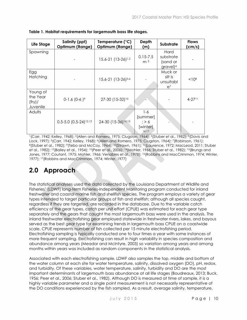
Table 1. Habitat requirements for largemouth bass life stages.

Life Stage Salinity (ppt)

Optimum (Range)

Temperature (°C)

Optimum (Range)

Depth

(m) Substrate

Flows

(cm/s)

Spawning

- 15.6-21 (13-26)1,2 0.15-7.5

m 3

Hard

substrate

(sand or

gravel)4

-

Egg

Hatching - 15.6-21 (13-26)5,6 -

Muck or

silt is

unsuitabl

e7

<108

Young of

the Year

(fry)/

Juvenile

0-1.6 (0-6 )9 27-30 (15-32)10 - - 4-2711

Adults

0.5-5.0 (0.5-24)12,13 24-30 (15-36)14,15

1-6

[summer]

; > 6

[winter] 16,17

- -

1(Carr, 1942; Kelley, 1968); 2(Allen and Romero, 1975; Clugston, 1964); 3(Stuber et al., 1982); 4(Davis and

Lock, 1997); 5(Carr, 1942; Kelley, 1968); 6(Allen and Romero, 1975; Clugston, 1964); 7(Robinson, 1961); 8(Stuber et al., 1982); 9(Tebo and McCoy, 1964); 10(Strawn, 1961); 11(Laurence, 1972; MacLeod, 2011; Stuber

et al., 1982); 12(Bailey et al., 1954); 13(Peer et al., 2006); 14(Mohler, 1966; Stuber et al., 1982); 15(Brungs and

Jones, 1977; Coutant, 1975; Mohler, 1966; Venables et al., 1978); 16(Robbins and MacCrimmon, 1974; Winter,

1977); 17(Robbins and MacCrimmon, 1974; Winter, 1977)

2.0 Approach

The statistical analyses used the data collected by the Louisiana Department of Wildlife and

Fisheries’ (LDWF) long-term Fisheries-Independent Monitoring program conducted for inland

freshwater and coastal marine fish and shellfish species. The program employs a variety of gear

types intended to target particular groups of fish and shellfish; although all species caught,

regardless if they are targeted, are recorded in the database. Due to the variable catch

efficiency of the gear types, catch per unit effort (CPUE) was estimated for each gear type

separately and the gears that caught the most largemouth bass were used in the analysis. The

inland freshwater electrofishing gear employed statewide in freshwater rivers, lakes, and bayous

served as the best gear type for examining trends in largemouth bass CPUE on a coastwide

scale. CPUE represents number of fish collected per 15 minute electrofishing period.

Electrofishing sampling is typically conducted one to four times a year with some instances of

more frequent sampling. Electrofishing can result in high variability in species composition and

abundance among years (Meador and McIntyre, 2003) so variation among years and among

months within years was included as random components in the statistical analysis.

Associated with each electrofishing sample, LDWF also samples the top, middle and bottom of

the water column at each site for water temperature, salinity, dissolved oxygen (DO), pH, redox,

and turbidity. Of these variables, water temperature, salinity, turbidity and DO are the most

important determinants of largemouth bass abundance at all life stages (Boudreaux, 2013; Buck,

1956; Peer et al., 2006; Stuber et al., 1982). Although DO is measured at time of sample, it is a

highly variable parameter and a single point measurement is not necessarily representative of

the DO conditions experienced by the fish sampled. As a result, average salinity, temperature,


J u l y 2 0 1 5 P a g e | 11

and turbidity were used for the analysis. The period of record for the LDWF water quality data at

electrofishing sites dates back to 1990 for a few sites but is readily available from hundreds of

sites statewide starting in the late 1990s/early 2000s. Thus, the analysis was conducted for those

time periods in which environmental data records were available, although biological records

(i.e., CPUE) may date back a decade earlier.

Additional parameters expected to influence largemouth bass include prey concentration and

emergent and aquatic vegetation. Suitability curves for these parameters were developed

based on literature and professional judgment. Thus, the statistical analysis presented here

focused on the development of quantitative relationships between largemouth bass and water

temperature, salinity, and turbidity. The resulting equations will be standardized to a 0 to 1 scale

in order to combine with the prey concentration and vegetation suitability index curves

(described in ‘Habitat Suitability Index Model’).

Within the electrofishing gear type, the length-frequency distributions were examined to

determine the life stages represented in the catch (Figure 3). Mature adults are > 260 mm total

length (TL; Boudreaux, 2013; Ludsin and DeVries, 1997). Approximately 65% of the individuals

were less than < 250 mm suggesting the samples comprised both juveniles/young of the year

(YOY) and adults. The habitat requirements for these life stages are not markedly different,

although adults have higher salinity tolerances than YOY (Table 1). However, given the interest in

developing a habitat suitability index model that is applicable to both adults and juveniles, the

dataset was not subset by size distribution.

Mean monthly CPUE by year for the species in the gear was also estimated and then plotted to

determine which months had the highest consistent catch over time and which months had

variable and low or no catch over time. These plots allowed for subsetting the data by the

months of highest species catch in order to reduce the amount of zeroes in the dataset. In this

way, the analysis was not focused on describing environmental effects on species catch when

the species typically are not present or else at very low numbers. Although largemouth bass are

present year round, they are most abundant March – November (Figure 4). Therefore, the

electrofishing data from March through November were used for the statistical evaluation of the

adult/juvenile largemouth bass CPUE-environment relationships.


J u l y 2 0 1 5 P a g e | 12

Figure 3. Length-frequency distribution (mm TL) of largemouth bass in electrofishing samples.

Figure 4. Mean catch per unit effort (CPUE) of largemouth bass in electrofishing samples.


J u l y 2 0 1 5 P a g e | 13

2.1 Statistical Analysis

The statistical approach was developed to predict mean CPUE in response to environmental

variables for multiple species of interest and was designed for systematic application across the

coast. The methods described in detail below rely on the use of polynomial regressions and

commonly-used SAS procedures that can be consistently and efficiently applied to fishery-

independent count data for species with different life histories and environmental tolerances. As

a result, the same statistical approach was used for each of the fish and shellfish species that are

being modeled with HSIs in the 2017 Master Plan. This was necessary due to time and resource

constraints on the overall model improvement effort. It is possible that an analysis focused solely

on largemouth bass would have identified an alternative approach.

The species CPUE data were transformed using ln(CPUE+1). Given that the sampling is

standardized and CPUE represent discrete values (total catch per sample event), ln(CPUE + 1)

transformation was appropriate for the analysis. Distributions that are reasonably symmetric

often give satisfactory results in parametric analyses, due in part to the effectiveness of the

Central Limit Theorem and in part to the robustness of regression analysis. Nevertheless, it is

expedient to approximate normality as closely as possible prior to conducting statistical

analyses. The negative binomial distribution is common for discrete distributions for samples

consisting of counts of organisms when the variance is greater than the mean. In these cases,

the natural logarithmic transformation is advantageous in de-emphasizing large values in the

upper tail of the distribution. As a result, the data were natural log-transformed for the analysis.

The transformation worked generally well in meeting the assumptions of the regression analysis.

Predictive models can often be improved by fitting some curvature to the variables by including

polynomial terms. This allows the rate of a linear trend to diminish as the variable increases or

decreases. It is expected that the largemouth bass may respond nonlinearly to salinity and

temperature (i.e., they have optimal values for biological processes; Glover et al., 2013). Thus,

polynomial regression was chosen for the analyses. Another consideration in modeling the

abundance of biota is the consistency of the effect of individual variables across the level of

other variables. The effect of temperature, for example, may not be consistent across all levels

of salinity. These changes can be modeled by considering interaction terms among the

independent variables in the polynomial regression equation.

Given the large number of potential variables and their interactions, it is prudent to use an

objective approach, such as stepwise procedures (Murtaugh, 2009), to select the variables for

inclusion in the development of the model. The SAS programming language has a relatively new

procedure called PROC GLMSelect, which is capable of performing stepwise selection where at

each step all variables are rechecked for significance and may be removed if no longer

significant. However, there are a number of limitations to PROC GLMSelect. GLMSelect is

intended primarily for parametric analysis where the assumption of a normal distribution is made.

It does not differentially handle random variables, so modern statistical techniques involving

random components, non-homogeneous variance and covariance structure cannot be used

with this technique. As a result, PROC GLMSelect was used as a ‘screening tool’ to identify the

key variables (linear, polynomial, and interactions), while the SAS procedure PROC MIXED was

used to calculate parameter estimates and ultimately develop the model. PROC MIXED is

intended primarily for parametric analyses, and can be used for regression analysis. Although it is

capable of fitting analyses with non-homogenous variances and other covariance structures,

the ultimate goal of the analysis was to predict mean CPUE, not for hypothesis testing or for

placing confidence intervals on the model estimates. The statistical significance levels for the

resulting parameters were used to evaluate whether the parameters of the polynomial

regression model adequately described the predicted mean (p<0.05).


J u l y 2 0 1 5 P a g e | 14

3.0 Results

The resulting polynomial regression model from the analysis describes largemouth bass CPUE

(natural log transformed) in terms of all significant effects from salinity, temperature, turbidity,

day of year, and their squared terms (Equation 1; Table 2). The model produces a dome-shape

relationship between CPUE and temperature, with highest CPUE occurring between 20-24°C

(Figure 5). Largemouth bass CPUE was also highest at lowest salinities and turbidities (Figure 6

and Figure 7). These responses agree with the ranges and optimums presented in Table 1.

Equation 1:

ln(CPUE + 1) = 0.8752 − 1.7125(𝐷𝑎𝑦) + 0.3768(𝐷𝑎𝑦2) − 0.2759(𝑆𝑎𝑙𝑖𝑛𝑖𝑡𝑦) + 0.007203(𝑆𝑎𝑙𝑖𝑛𝑖𝑡𝑦2)

+ 0.3328(𝑇𝑒𝑚𝑝𝑒𝑟𝑎𝑡𝑢𝑟𝑒) − 0.0406(𝑇𝑢𝑟𝑏𝑖𝑑𝑖𝑡𝑦) − 0.00764(𝑇𝑒𝑚𝑝𝑒𝑟𝑎𝑡𝑢𝑟𝑒2)

+ 0.000632(𝑇𝑢𝑟𝑏𝑖𝑑𝑖𝑡𝑦2)

Table 2. List of selected effects with parameter estimates and their level of significance for the

resulting polynomial regression in Equation 1.

Selected Effects Parameter Estimate1 p value

Intercept 0.8752 0.4897

Day -1.7125 0.0683

Day2 0.3768 0.1029

Turbidity -0.04060 0.0002

Turbidity2 0.000632 0.0043

Salinity -0.2759 <.0001

Salinity2 0.007203 <.0001

Temperature 0.3328 0.0003

Temperature2 -0.00764 0.0001

1 Significant figures may vary among parameters due to rounding or accuracy of higher order

terms.


J u l y 2 0 1 5 P a g e | 15

Figure 5. Predicted output from polynomial regression in Equation 1 over the range of

temperatures values. Observed values of temperature and ln(CPUE+1) are overlaid.

Figure 6. Predicted output from polynomial regression in Equation 1 over the range of salinity

values. Observed values of salinity and ln(CPUE+1) are overlaid.


J u l y 2 0 1 5 P a g e | 16

Figure 7. Predicted output from polynomial regression in Equation 1 over the range of turbidity

values (in Nephelometric Turbidity Units [NTU]). Observed values of turbidity and ln(CPUE+1) are

overlaid.

4.0 Habitat Suitability Index Model for Juvenile and Adult

Largemouth Bass

Although the polynomial regression function in Equation 1 appears long and complex, the

regression model is simply describing the relationship among largemouth bass catch from

electrofishing and the salinity, temperature, and turbidity taken with the samples. In order to use

the polynomial regression (Equation 1) as an HSI model, the equation was standardized to a 0-1

scale. Standardization of the equation was performed by first back-transforming the predicted

CPUE [ln(CPUE+1)] to untransformed CPUE values. The predicted untransformed CPUE values

were then standardized by the maximum predicted (untransformed) CPUE value from the

response function. Maximum CPUE was calculated by running the polynomial model through

salinity, temperature, and turbidity combinations that fall within plausible ranges.

A predicted maximum largemouth bass ln(CPUE+1) value of 2.903 was generated from the

polynomial regression at a temperature of 22 °C, salinity of 0 ppt, and turbidity of 0 NTU. The

back-transformed CPUE value (17.225) was used to standardize the other predicted

untransformed CPUE values from the regression. The resulting standardized water quality

suitability index was combined with a standardized (0-1) index for emergent and submerged

aquatic vegetation and a standardized index for Chlorophyll a concentration (used as a proxy

for prey availability) to produce the HSI model. All three components of the model are equally

weighted and the geometric mean is used as all variables are considered essential to juvenile

and adult largemouth bass.


J u l y 2 0 1 5 P a g e | 17

HSI = (SI1 * SI2 * SI3)1/3

Where:

SI1 – Suitability index for juvenile and adult largemouth bass in relation to salinity, temperature,

and turbidity during the months of March through November (V1)

SI2 – Suitability index for juvenile and adult largemouth bass in relation to the percent of the cell

that is emergent vegetation and submerged aquatic vegetation (V2)

SI3 – Suitability index for juvenile and adult largemouth bass in relation to the Chlorophyll a

concentrations of the cell (V3)

4.1 Applicability of the Model

The model is applicable for calculating annual habitat suitability index for juvenile and adult

largemouth bass (median size about 200 mm TL from Figure 3) from March through November in

low-salinity estuarine habitats (e.g., ponds, lakes, bayous) of Louisiana.

4.2 Response and Input Variables

V1: Salinity, temperature, and turbidity during the months of March through November

Calculate monthly averages of salinity (ppt), temperature (°C), and turbidity (NTU) from March

through November:

𝑉1 = 0.8752 − 1.7125(1.99) + 0.3768(4.808) − 0.2759(𝑆𝑎𝑙𝑖𝑛𝑖𝑡𝑦) + 0.007203(𝑆𝑎𝑙𝑖𝑛𝑖𝑡𝑦2)

+ 0.3328(𝑇𝑒𝑚𝑝𝑒𝑟𝑎𝑡𝑢𝑟𝑒) − 0.0406(𝑇𝑢𝑟𝑏𝑖𝑑𝑖𝑡𝑦) − 0.00764(𝑇𝑒𝑚𝑝𝑒𝑟𝑎𝑡𝑢𝑟𝑒2)

+ 0.000632(𝑇𝑢𝑟𝑏𝑖𝑑𝑖𝑡𝑦2)

The resulting suitability index (SI1) should then be calculated as:

𝑆𝐼1 =𝑒𝑉1 − 1

17.225

which includes the steps for back-transforming the predicted CPUE from Equation 1 and

standardizing by the maximum predicted (untransformed) CPUE value equal to 12.214. The

suitability index curves that describe the standardized juvenile and adult largemouth bass

response (0-1) to individual effects of salinity, temperature, and turbidity are shown in Figure 8

through Figure 10.

Rationale: Salinity, temperature, and turbidity are important abiotic factors that can influence

the spatial and temporal distribution of largemouth bass within a year. The suitability index

resulted from the polynomial regression model that described the fit to the observed catch data

in relation to the salinity, temperature, and turbidity measurements taken by the LDWF

electrofishing samples. The resulting suitability index predicts salinity, temperature, and turbidity

ranges and optimums (Figure 8 - Figure 10) that agree well with the ranges and optimums

previously described in the literature for juvenile and adult largemouth bass (see Table 1).

Largemouth bass are generally found in low salinity environments < 5 ppt, but have also been

shown to be tolerant of salinities up to 12 ppt (Peer et al., 2006). Temperature plays a key role in


J u l y 2 0 1 5 P a g e | 18

the success of spawning adults and ultimately egg survival. Previous studies have shown

optimum temperatures between 15°C and 30°C (see Table 1). Largemouth bass are visual

piscivores; thus, high turbidity may limit growth and reproductive success via reduction in

foraging success (McMahon & Holanov, 1995).

Limitations: The variable ‘day’ in Equation 1 has been replaced by a constant value equal to the

mean day from the analysis (July 18)2. Holding ‘day’ constant prevents the variable from

contributing to the within- or among-year variation, so that only salinity, temperature, and

turbidity can vary within and among years. The salinity suitability index was adjusted to reflect

zero suitability for salinity greater than 20 ppt in order to prevent the model from placing the

species in high salinity areas. Similarly, the turbidity suitability index was truncated at 32 NTU, such

that all predictions at higher tur100bidity values are equal to those at turbidity of 32 NTU.


to temperature, with all other variables held constant at their optimum values, and resulting from

the back-transformation and standardization of the polynomial regression in Equation 1.

2 Day of the year is scaled between 1 and 3.65 (i.e., 365/100) because the coefficients for higher power

terms get exceedingly small and often do not have many significant digits. For example, a coefficient of

0.00004 may actually be 0.0000351 and that can make a big difference when multiplied by 365 raised to

the power of 2. By using a smaller value, decimal precision is improved.


J u l y 2 0 1 5 P a g e | 19


to salinity, with all other variables held constant at their optimum values, and resulting from the

back-transformation and standardization of the polynomial regression in Equation 1.

Figure 10. Graph demonstrating the predicted suitability index (0-1) for largemouth bass in

relation to turbidity, with all other variables held constant at their optimum values, and resulting

from the back-transformation and standardization of the polynomial regression in Equation 1.

V2: Percent of cell that is covered by land and including all types of vegetation

Calculate the percent of the (500 X 500 m) cell that is covered by emergent vegetation types

and submerged aquatic vegetation combined to derive V2 for the suitability index (SI2). The

equation for SI2 is plotted in Figure 11. The index is calculated as:


J u l y 2 0 1 5 P a g e | 20

SI2 = 0.01 for V2 < 20

0.099 * V1-1.97 for 20 ≤ V2 < 30

1.0 for 30 ≤ V2 < 50

-0.0283*V1+2.414 for 50 ≤ V2 < 85

0.01 for 85 ≤ V2 < 100

0 for V2 = 100

Figure 11. The suitability index for largemouth bass in relation to the % emergent vegetation and

submerged aquatic vegetation (V2).

Rationale: Emergent and submerged aquatic vegetation: (1) provide foraging opportunities for

juveniles and adults that feed on insects, fish, and other invertebrates, (2) provide protection to

juveniles from larger predators, and (3) may serve as potential spawning habitat for adults.

Given that the functions they provide to juvenile and adult largemouth bass are similar, it is

recommended the suitability index developed in the 2012 Master Plan for emergent vegetation

(see Appendix D9 in CPRA, 2012), be used to represent both emergent vegetation and SAV. This

assumes that the presence of SAV is equal to that of emergent vegetation and that the

presence of either (or both) at intermediate levels (i.e., 30-50%) provide suitable habitat. Given

that the absence of vegetation does not lead to direct mortality, the minimum suitability index is

0.01. This prevents the overall HSI model from equaling zero when vegetation is absent.

Limitations: None.

V3: Chlorophyll a concentration of the cell

Calculate the Chlorophyll a concentration of the (500 X 500 m) cell and substitute V3 into the

suitability index (SI3). The equation for SI3 is plotted in Figure 11. The index is calculated as:


J u l y 2 0 1 5 P a g e | 21

𝑆𝐼3 = 0.24 +0.85

1 + 𝑒−𝑉3−35.75

7.8414

Figure 12. The suitability index for largemouth bass in relation to the Chlorophyll a concentration

(Chlorophyll a = V3).

Rationale: The sigmoidal feeding response function best fit the largemouth bass suitability index

presented in the 2012 Master Plan. Increased Chlorophyll a concentrations have an indirect

effect on juvenile and adult largemouth bass in that it is indicative of high primary productivity

and foraging opportunities for largemouth bass prey (e.g., insects, fish, and other invertebrates).

As a result, high Chlorophyll a concentrations should result in high food availability for

largemouth bass. The SI3 equation was modified from the 2012 Master Plan to better represent

the sigmoidal shape of the curve, however, the overall relationship remains largely unchanged.

No additional literature and data for which to make further improvements were available.

Limitations: The relationship assumes that largemouth bass habitat suitability is directly related to

Chlorophyll a concentration.

5.0 Model Verification and Future Improvements

A verification exercise was conducted to ensure the distributions and patterns of HSI scores

across the coast were realistic relative to current knowledge of the distribution of largemouth

bass. In order to generate HSI scores across the coast, the HSI model was run using calibrated

and validated ICM spin-up data to produce a single value per ICM grid cell. Given the natural

internannual variation in salinity patterns across the coast, several years of model output were

examined to evaluate the internannual variability in the HSI scores. An accurate representation

of algae in the system was not available as inputs to generate a chlorophyll a suitability index

score, and thus SI3 was held constant at 1 for all model runs. Further, a universal equation

applicable to the entire coast could not be generated to convert turbidity (in NTU) to TSS in

order to link the HSI model to the hydrology subroutine. As a result, the turbidity was held

constant at 0 (i.e., the optimum value in the polynomial equation) for all model runs.


J u l y 2 0 1 5 P a g e | 22

For the largemouth bass model, high scores were observed around low salinity areas with

fragmented marsh or SAV, such as those within Barataria, Breton, and the Atchafalaya. Scores

were lowest in open water bodies closest to the Gulf of Mexico such as Chandeleur Sound and

Terrebonne Bay. A limitation of this model is there are no geographic constraints that prevent

the model from generating HSI scores in areas where the species are not likely to occur. For

example, habitat in certain areas may be highly suitable but likely may never be occupied due

to accessibility constraints (e.g., impounded wetlands). Overall, the results of the verification

exercise were determined to be accurate representations largemouth bass distributions in

coastal Louisiana.

Although the polynomial regression model used to fit the LDWF electrofishing data produced

functions relating largemouth bass catch to salinity, temperature, and turbidity that generally

agreed with their life history information and distributions (Pattillo et al., 1997), polynomial models

can predict unreasonable results outside of the modeled data range. Other statistical methods

and modeling techniques exist for fitting nonlinear relationships among species catch and

environmental data that could potentially improve the statistical inferences and model behavior

outside of the available data. A review of other statistical modeling techniques could be

conducted in order to determine their applicability in generating improved HSI models in the

future.


J u l y 2 0 1 5 P a g e | 23

6.0 References

Allen, R. C., and Romero, J. (1975). Underwater Observations of Largemouth Bass Spawning and

Survival in Lake Mead. In H. Clepper (editor), Black Bass Biology and Management (pp

104-112). Washington D.C.: Sport Fishing Institute.

Bailey, R. M., Winn, H. E., and Smith, C. L. (1954). Fishes from the Escambia River, Alabama and

Florida, with ecologic and taxonomic notes. Proceedings of the Academy of Natural

Sciences of Philadelphia, 106, 109–164.

Boudreaux, B. A. (2013). Assessment of Largemouth Bass Micropterus salmoides Age, Growth,

Gonad Development and Diet in the Upper Barataria Estuary (Master of Science in

Marine and Environmental Biology). Nicholls State University. Retrieved from

http://www.nicholls.edu/bayousphere/GraduateStudents/BBoudreaux/BoThesis(Final).pd

f

Brown, T. J., Runciman, B., Polllard, S., and Grant, A. D. A. (2009). Biological Synopsis of

Largemouth Bass (Micropterus salmoides). Canadian Manuscript Report of Fisheries and

Aquatic Sciences No. 2884. British Columbia: Fisheries and Oceans Canada.

Brungs, W. A., and Jones, B. R. (1977). Temperature criteria for freshwater fish: Protocol and

procedures (No. EPA-600/3-77-061). Duluth, Minnesota: Environmental Research

Laboratory, U.S. Environmental Protection Agency.

Buck, D. H. (1956). Effects of turbidity on fish and fishing. Norman, Oklahoma: Oklahoma Fisheries

Research Laboratory,. Retrieved from

http://www.biodiversitylibrary.org/bibliography/20235

Carr, M. H. (1942). The breeding habits, embryology and larval development of the

largemouthed black bass in Florida. Proceedings of the New England Zoological Club,

20, 48–77.

Chen, R. J., Hunt, K. M., and Ditton, R. B. (2003). Estimating the economic impacts of a trophy

largemouth bass fishery: issues and applications. North American Journal of Fisheries

Management, 23(3), 835–844.

Clugston, J. P. (1964). Growth of the Florida Largemouth Bass, Micropterus salmoides floridanus

(LeSueur), and the Northern Largemouth Bass, M. s. salmoides (Lacépède), in Subtropical

Florida. Transactions of the American Fisheries Society, 93(2), 146–154.

Coastal Protection and Restoration Authority (CPRA) (2012). Louisiana’s Comprehensive Master

Plan for a Sustainable Coast. Baton Rouge, LA: CPRA, p. 186.

Coutant, C. C. (1975). Responses of bass to natural and artificial temperature regimes. Oak

Ridge National Lab., Tenn.(USA). Retrieved from

http://www.osti.gov/scitech/biblio/4235116

Davis, J. T., and Lock, J. T. (1997). Largemouth bass biology and life history (SRAC Publication No.

200). Southern Regional Aquaculture Center.


J u l y 2 0 1 5 P a g e | 24

Diana, M. J., and Wahl, D. H. (2008). Long-term stocking success of largemouth bass and the

relationship to natural populations. In Balancing fisheries management and water uses

for impounded river systems. (Vol. 62, pp. 413–426). Bethesda, Maryland.

Glover, D. C., DeVries, D. R., and Wright, R. A. (2013). Growth of largemouth bass in a dynamic

estuarine environment: an evaluation of the relative effects of salinity, diet, and

temperature. Canadian Journal of Fisheries and Aquatic Sciences, 70(3), 485–501.

Goodgame, L. S., and Miranda, L. E. (1993). Early Growth and Survival of Age-0 Largemouth Bass

in Relation to Parental Size and Swim-up Time. Transactions of the American Fisheries

Society, 122(1), 131–138.

Hodgson, J. R., Hodgson, C. J., and Hodgson, J. Y. S. (2008). Water Mites in the Diet of

Largemouth Bass. Journal of Freshwater Ecology, 23(2), 327–331.

Kazumi, H., and Keita, N. (2003). Bibliography on largemouth bass and smallmouth bass, the

invasive alien fishes to Japan. Memoirs of the Faculty of Agriculture of Kinki University.

Retrieved from http://sciencelinks.jp/j-east/article/200315/000020031503A0456680.php

Kelley, J. W. (1968). Effects of Incubation Temperature on Survival of Largemouth Bass Eggs. The

Progressive Fish-Culturist, 30(3), 159–163.

Lasenby, T. A., and Kerr, S. J. (2000). Bass stocking and transfers: An annotated bibliography and

literature review. Peterborough, Ontario: Fish and Wildlife Branch, Ontario Ministry of

Natural Resources.

Laurence, G. C. (1972). Comparative swimming abilities of fed and starved larval largemouth

bass (Micropterus salmoides). Journal of Fish Biology, 4(1), 73–78.

Ludsin, S. A., and DeVries, D. R. (1997). First-Year Recruitment of Largemouth Bass: The

Interdependency of Early Life Stages. Ecological Applications, 7(3), 1024–1038.

Maceina, M. J. (1996). Largemouth bass abundance and aquatic vegetation in Florida lakes: an

alternative interpretation. Journal of Aquatic Plant Management, 34, 43–47.

MacLeod, J. C. (2011). A new apparatus for measuring maximum swimming speeds of small fish.

Journal of the Fisheries Research Board of Canada, 24(6), 1241–1252.

McMahon, T. E., and Holanov, S. H. (1995). Foraging success of largemouth bass at different light

intensities: implications for time and depth of feeding. Journal of Fish Biology, 46(5), 759–

767.

McPhail, J. D., and McPhail, D. L. (2007). The freshwater fishes of British Columbia. Edmonton:

University of Alberta Press.

Meador, M. R., and McIntyre, J. P. (2003). Effects of Electrofishing Gear Type on Spatial and

Temporal Variability in Fish Community Sampling. Transactions of the American Fisheries

Society, 132(4), 709–716.

Miranda, L. E., and Pugh, L. L. (1997). Relationship between vegetation coverage and

abundance, size, and diet of juvenile largemouth bass during winter. North American

Journal of Fisheries Management, 17(3), 601–610.


J u l y 2 0 1 5 P a g e | 25

Mohler, H. S. (1966). Comparative seasonal growth of the largemouth, spotted and smallmouth

bass. M.A. Thesis. University of Missouri. 99 pp.

Murtaugh, P. A. (2009). Performance of several variable-selection methods applied to real

ecological data. Ecology Letters, 12(10), 1061-1068.

Peer, A. C., DeVries, D. R., and Wright, R. A. (2006). First-year growth and recruitment of coastal

largemouth bass (Micropterus salmoides): Spatial patterns unresolved by critical periods

along a salinity gradient. Canadian Journal of Fishereis and Aquatic Sciences, 63, 1911–

1924.

Philipp, D. P., Childers, W. F., and Whitt, G. S. (1983). A biochemical genetic evaluation of the

northern and Florida subspecies of largemouth bass. Transactions of the American

Fisheries Society, 112(1), 1-20.

Post, D. M. (2003). Individual Variation in the Timing of Ontogenetic Niche Shifts in Largemouth

Bass. Ecology, 84(5), 1298–1310.

Robbins, W. H., and MacCrimmon, H. R. (1974). The blackbass in America and overseas. Sault

Sainte Marie, Ont.: Biomanagement and Research Enterprises.

Robinson, D. W. (1961). Utilization of Spawning Box by Bass. The Progressive Fish-Culturist, 23(3),

119–119.

Scott, W. B., and Crossman, E. J. (1973). Freshwater Fishes of Canada. Fisheries Research Board of

Canada.

Stein, J. N. (1970). A study of the largemouth bass population in Lake Washington. Master’s thesis.

University of Washington, Seattle.

Strawn, K. (1961). Growth of Largemouth Bass Fry at Various Temperatures. Transactions of the

American Fisheries Society, 90(3), 334–335.

Stuber, R. J., Gebhart, G., and Maughan, O. E. (1982). Habitat suitability index models:

Largemouth bass. U.S. Dept. Int. Fish Wildlife Service.

Tebo, L. B., and McCoy, E. G. (1964). Effect of Sea-Water Concentration on the Reproduction

and Survival of Largemouth Bass and Bluegills. The Progressive Fish-Culturist, 26(3), 99–106.

Venables, B. J., Fitzpatrick, L. C., and Pearson, W. D. (1978). Laboratory measurement of

preferred body temperature of adult largemouth bass (Micropterus salmoides).

Hydrobiologia, 58(1), 33–36.

Winter, J. D. (1977). Summer home range movements and habitat use by four largemouth bass in

Mary Lake, Minnesota. Transactions of the American Fisheries Society, 106(4), 323–330.

appendix c modeling attachment c3-18 - coastal...

Documents