Appendix W

Dynamic Models

W.2 4 Complex Mechanical Systems

W.2.1 Translational and Rotational SystemsIn some cases, mechanical systems contain both translational and rotational portions. The procedureis the same as that described in Section 2.1: sketch the free-body diagrams, de�ne coordinates andpositive directions, determine all forces and moments acting, and apply Eqs. (2.1) and/or (2.14).

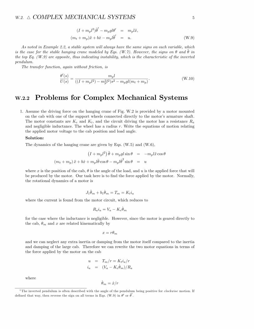
Example W.1 Rotational and Translational Motion: Hanging Crane Write the equationsof motion for the hanging crane pictured in Fig. W.1 and shown schematically in Fig. W.2. Linearizethe equations about � = 0, which would typically be valid for the hanging crane. Also linearize theequations for � = �, which represents the situation for the inverted pendulum shown in Fig. W.3.SOLUTION A schematic diagram of the hanging crane is shown in Fig. W.2 while the free-body

diagrams are shown in Fig. W.4. In the case of the pendulum, the forces are shown with bold lines,while the components of the inertial acceleration of its center of mass are shown with dashed lines.Because the pivot point of the pendulum is not �xed with respect to an inertial reference, the rotationof the pendulum and the motion of its mass center must be considered. The inertial acceleration needsto be determined because the vector a in Eq. (2.1) is given with respect to an inertial reference. Theinertial acceleration of the pendulum�s mass center is the vector sum of the three dashed arrows shownin Fig. W.4(b). The derivation of the components of an object�s acceleration is called kinematicsand is usually studied as a prelude to the application of Newton�s laws. The results of a kinematicstudy are shown in Fig. W.4(b). The component of acceleration along the pendulum is l _�

2and is

called the centripetal acceleration. It is present for any object whose velocity is changing direction.The �x-component of acceleration is a consequence of the pendulum pivot point accelerating at thetrolley�s acceleration and will always have the same direction and magnitude as those of the trolley�s.The l�� component is a result of angular acceleration of the pendulum and is always perpendicular tothe pendulum.These results can be con�rmed by expressing the center of mass of the pendulum as a vector from

an inertial reference and then di¤erentiating that vector twice to obtain an inertial acceleration.Figure W.4(c) shows i and j axes which are inertially �xed and a vector r describing the position ofthe pendulum center of mass. The vector can be expressed as

r = xi+ l(i sin � � j cos �):

The �rst derivative of r is_r = _xi+ l _�(i cos � + j sin �):

Likewise, the second derivative of r is

�r = �xi+ l��(i cos � + j sin �)� l _�2(i sin � � j cos �):

1

2 APPENDIX W. DYNAMIC MODELS

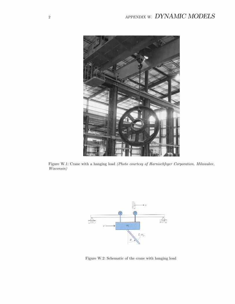
Figure W.1: Crane with a hanging load (Photo courtesy of Harnischfeger Corporation, Milwaukee,Wisconsin)

Figure W.2: Schematic of the crane with hanging load

W.2. 4 COMPLEX MECHANICAL SYSTEMS 3

Figure W.3: Inverted pendulum

Figure W.4: Hanging crane: (a) free-body diagram of the trolley; (b) free-body diagram of thependulum; (c) position vector of the pendulum

4 APPENDIX W. DYNAMIC MODELS

Note that the equation for �r con�rms the acceleration components shown in Fig.W.4(b). The l _�2

term is aligned along the pendulum pointing toward the axis of rotation and the l�� term is alignedperpendicular to the pendulum pointing in the direction of a positive rotation.Having all the forces and accelerations for the two bodies, we now proceed to apply Eq. (2.1). In

the case of the trolley, Fig.W.4(a), we see that it is constrained by the tracks to move only in thex-direction; therefore, application of Eq. (2.1) in this direction yields

mt�x+ b _x = u�N; (W.1)

where N is an unknown reaction force applied by the pendulum. Conceptually, Eq. (2.1) can beapplied to the pendulum of Fig. W.4(b) in the vertical and horizontal directions, and Eq. (2.14) canbe applied for rotational motion to yield three equations in the three unknowns: N , P , and �. Thesethree equations can then be manipulated to eliminate the reaction forces N and P so that a singleequation results describing the motion of the pendulum� that is, a single equation in �. For example,application of Eq. (2.1) for pendulum motion in the x-direction yields

N = mp�x+mpl�� cos � �mpl _�2sin �: (W.2)

However, considerable algebra will be avoided if Eq. (2.1) is applied perpendicular to the pendulumto yield

P sin � +N cos � �mpg sin � = mpl�� +mp�x cos �: (W.3)

Application of Eq. (2.14) for the rotational pendulum motion, for which the moments are summedabout the center of mass, yields

�Pl sin � �Nl cos � = I��; (W.4)

where I is the moment of inertia about the pendulum�s mass center. The reaction forces N and Pcan now be eliminated by combining Eqs. (W.3) and (W.4). This yields the equation

(I +mpl2)�� +mpgl sin � = �mpl�x cos �: (W.5)

It is identical to a pendulum equation of motion, except that it contains a forcing function that isproportional to the trolley�s acceleration.An equation describing the trolley motion was found in Eq. (W.1), but it contains the unknown

reaction force N . By combining Eqs. (W.2) and (W.1), N can be eliminated to yield

(mt +mp)�x+ b _x+mpl�� cos � �mpl _�2sin � = u: (W.6)

Equations (W.5) and (W.6) are the nonlinear di¤erential equations that describe the motion of thecrane with its hanging load. For an accurate calculation of the motion of the system, these nonlinearequations need to be solved.

To linearize the equations for small motions about � = 0, let cos � �= 1, sin � �= �, and _�2 �= 0;

thus the equations are approximated by

(I +mpl2)�� +mpgl� = �mpl�x;

(mt +mp)�x+ b _x+mpl�� = u: (W.7)

Neglecting the friction term b leads to the transfer function from the control input u to hangingcrane angle �:

�(s)

U(s)=

�mpl

((I +mpl2)(mt +mp)�m2pl2)s2 +mpgl(mt +mp)

: (W.8)

For the inverted pendulum in Fig. W.3, where � �= �, assume � = � + �0, where �0 representsmotion from the vertical upward direction. In this case, cos � �= �1, sin � �= ��0 in Eqs. (W.5) and(W.6), and Eqs. (W.7) become1Inverted pendu-

lum equations

W.2. 4 COMPLEX MECHANICAL SYSTEMS 5

(I +mpl2)��

0 �mpgl�0 = mpl�x;

(mt +mp)�x+ b _x�mpl��0= u: (W.9)

As noted in Example 2.2, a stable system will always have the same signs on each variable, whichis the case for the stable hanging crane modeled by Eqs. (W.7). However, the signs on � and �� inthe top Eq. (W.9) are opposite, thus indicating instability, which is the characteristic of the invertedpendulum.The transfer function, again without friction, is

�0(s)

U(s)=

mpl

((I +mpl2)�m2pl2)s2 �mpgl(mt +mp)

: (W.10)

W.2.2 Problems for Complex Mechanical Systems

1. Assume the driving force on the hanging crane of Fig. W.2 is provided by a motor mountedon the cab with one of the support wheels connected directly to the motor�s armature shaft.The motor constants are Ke and Kt, and the circuit driving the motor has a resistance Raand negligible inductance. The wheel has a radius r. Write the equations of motion relatingthe applied motor voltage to the cab position and load angle.

Solution:

The dynamics of the hanging crane are given by Eqs. (W.5) and (W.6),�I +mpl

2��� +mpgl sin � = �mpl�x cos �

(mt +mp) �x+ b _x+mpl�� cos � �mpl _�2sin � = u

where x is the position of the cab, � is the angle of the load, and u is the applied force that willbe produced by the motor. Our task here is to �nd the force applied by the motor. Normally,the rotational dynamics of a motor is

J1��m + b1 _�m = Tm = Ktia

where the current is found from the motor circuit, which reduces to

Raia = Va �Ke_�m

for the case where the inductance is negligible. However, since the motor is geared directly tothe cab, �m and x are related kinematically by

x = r�m

and we can neglect any extra inertia or damping from the motor itself compared to the inertiaand damping of the large cab. Therefore we can rewrite the two motor equations in terms ofthe force applied by the motor on the cab

u = Tm=r = Ktia=r

ia = (Va �Ke_�m)=Ra

where_�m = _x=r

1The inverted pendulum is often described with the angle of the pendulum being positive for clockwise motion. Ifde�ned that way, then reverse the sign on all terms in Eqs. (W.9) in �0 or ��

0.

6 APPENDIX W. DYNAMIC MODELS

These equations, along with �I +mpl

2��� +mpgl sin � = �mpl�x cos �

(mt +mp) �x+ b _x+mpl�� cos � �mpl _�2sin � = u

constitute the required relations.

2. Assume the driving force on the hanging crane of Fig. W.2 is provided by a motor mountedon the cab with one of the support wheels connected directly to the motor�s armature shaft.The motor constants are Ke and Kt, and the circuit driving the motor has a resistance Raand negligible inductance. The wheel has a radius r. Write the equations of motion relatingthe applied motor voltage to the cab position and load angle.