application note feedback control tuning with motion
TRANSCRIPT
APPLICATIONNOTE 151
13.12.2017 Page 1 of 28
Application Note – Feedback Control Tuning with
Motion Manager 6.3 or higher
Summary
To get the best performance out of your positioning system the feedback control parameters of
the FAULHABER Motion Controller have to be adjusted to the application.
This application note describes the tuning of the feedback control parameters of the
FAULHABER Motion Controllers via Motion Manager 6.3 or higher.
Concerning
The following products: MC5010, MC5005, MC5004 and MCS
Content
Page 2 Motivation – Goals of the Tuning
Page 5 Prerequisites for Feedback Control Tuning
Page 7 Feedback Control Tuning - the Tool – the software tool will be explained
Page 11 Step by Step Instruction– the actual Tuning is done here!
Page 20 Appendix with Troubleshooting, Expert Tuning and additional hints
Additional information and details have a green colored background.
An Overview of the next tuning steps is marked with a blue background color.
Faulhaber Application Note 151 Page 2 of 28
Motivation
This application note provides a step by step instruction how to tune the controllers in an efficient
way, which reduces the commissioning time significantly compared to a trial and error approach.
First of all you should have a clear idea of your own tuning goals.
Controller Tuning can have different goals, for instance:
- Reaching the target position without overshoot
- Fast command response
- Good disturbance rejection
- Silent motor run
- …
The individual goals have to be weighted, as not all can be achieved with the same set of
parameters. A system which is tuned for high dynamics will not necessarily run very silently at
the same time.
Tuning goal of this application note
This application note focuses on the tuning goal of “fast command response with very little or no
position overshoot”. In addition the underlying velocity loop will be tuned to minimize
disturbances, with a focus on positioning applications, like x-y stages, which would benefit from
these criteria.
Faulhaber Application Note 151 Page 3 of 28
Motivation - Continued
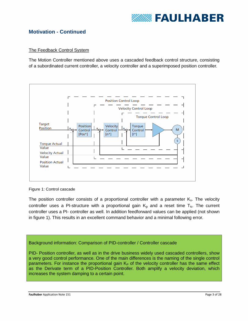
The Feedback Control System
The Motion Controller mentioned above uses a cascaded feedback control structure, consisting
of a subordinated current controller, a velocity controller and a superimposed position controller.
Figure 1: Control cascade
The position controller consists of a proportional controller with a parameter Kv. The velocity
controller uses a PI-structure with a proportional gain Kp and a reset time TN. The current
controller uses a PI- controller as well. In addition feedforward values can be applied (not shown
in figure 1). This results in an excellent command behavior and a minimal following error.
Background information: Comparison of PID-controller / Controller cascade PID- Position controller, as well as in the drive business widely used cascaded controllers, show a very good control performance. One of the main differences is the naming of the single control parameters. For instance the proportional gain KP of the velocity controller has the same effect as the Derivate term of a PID-Position Controller. Both amplify a velocity deviation, which increases the system damping to a certain point.
Faulhaber Application Note 151 Page 4 of 28
Motivation - Continued
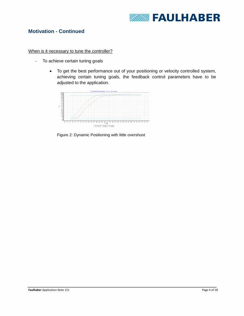
When is it necessary to tune the controller?
- To achieve certain tuning goals
To get the best performance out of your positioning or velocity controlled system,
achieving certain tuning goals, the feedback control parameters have to be
adjusted to the application.
Figure 2: Dynamic Positioning with little overshoot

Faulhaber Application Note 151 Page 5 of 28
Prerequisites for Feedback Control Tuning
The Tuning methods introduced in this application note require the system to fulfill the following
conditions:
- The system has to be complete, including the power supply
If there will be any significant system changes the feedback control tuning has to be repeated.
- The motor has to be set using the motor selection wizard
Figure 3: Wizard for motor selection
Here the current controller will be adjusted automatically based on the motor data. It is not meant to be tuned manually. Incorrect current controller settings will damage the motor or the power stage.
In addition the overvoltage threshold is set according to the voltage supplied to Umot (see page 25 for details).
Faulhaber Application Note 151 Page 6 of 28
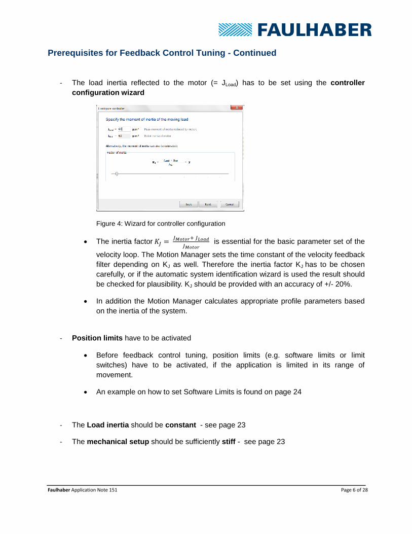
Prerequisites for Feedback Control Tuning - Continued
- The load inertia reflected to the motor (= JLoad) has to be set using the controller
configuration wizard
Figure 4: Wizard for controller configuration
The inertia factor 𝐾𝐽 = 𝐽𝑀𝑜𝑡𝑜𝑟+ 𝐽𝐿𝑜𝑎𝑑
𝐽𝑀𝑜𝑡𝑜𝑟 is essential for the basic parameter set of the
velocity loop. The Motion Manager sets the time constant of the velocity feedback
filter depending on KJ as well. Therefore the inertia factor KJ has to be chosen
carefully, or if the automatic system identification wizard is used the result should
be checked for plausibility. KJ should be provided with an accuracy of +/- 20%.
In addition the Motion Manager calculates appropriate profile parameters based
on the inertia of the system.
- Position limits have to be activated
Before feedback control tuning, position limits (e.g. software limits or limit
switches) have to be activated, if the application is limited in its range of
movement.
An example on how to set Software Limits is found on page 24
- The Load inertia should be constant - see page 23
- The mechanical setup should be sufficiently stiff - see page 23
Faulhaber Application Note 151 Page 7 of 28
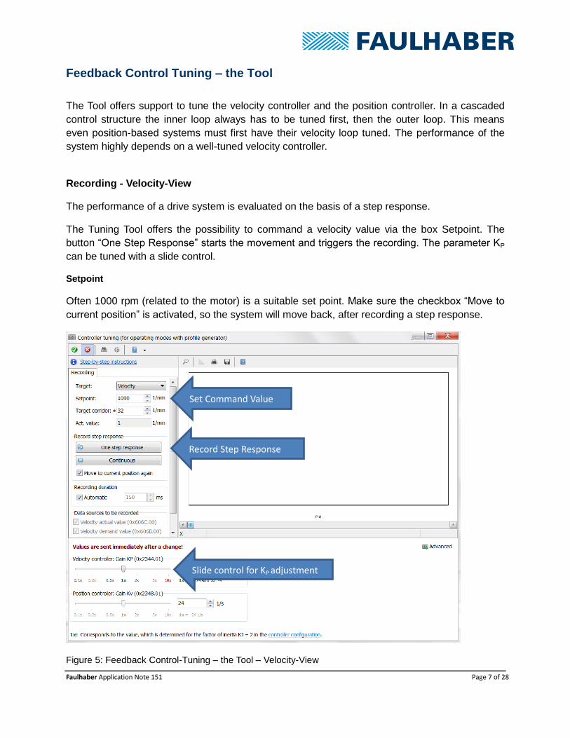
Feedback Control Tuning – the Tool
The Tool offers support to tune the velocity controller and the position controller. In a cascaded
control structure the inner loop always has to be tuned first, then the outer loop. This means
even position-based systems must first have their velocity loop tuned. The performance of the
system highly depends on a well-tuned velocity controller.
Recording - Velocity-View
The performance of a drive system is evaluated on the basis of a step response.
The Tuning Tool offers the possibility to command a velocity value via the box Setpoint. The
button “One Step Response” starts the movement and triggers the recording. The parameter KP
can be tuned with a slide control.
Setpoint
Often 1000 rpm (related to the motor) is a suitable set point. Make sure the checkbox “Move to
current position” is activated, so the system will move back, after recording a step response.
Figure 5: Feedback Control-Tuning – the Tool – Velocity-View
Set Command Value
Record Step Response
Slide control for KP adjustment
Faulhaber Application Note 151 Page 8 of 28
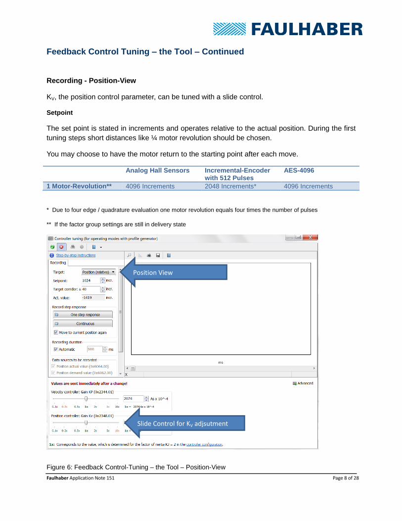
Feedback Control Tuning – the Tool – Continued
Recording - Position-View
KV, the position control parameter, can be tuned with a slide control.
Setpoint
The set point is stated in increments and operates relative to the actual position. During the first
tuning steps short distances like ¼ motor revolution should be chosen.
You may choose to have the motor return to the starting point after each move.
Analog Hall Sensors Incremental-Encoder with 512 Pulses
AES-4096
1 Motor-Revolution** 4096 Increments 2048 Increments* 4096 Increments
* Due to four edge / quadrature evaluation one motor revolution equals four times the number of pulses
** If the factor group settings are still in delivery state
Figure 6: Feedback Control-Tuning – the Tool – Position-View
Slide Control for KV adjsutment
Position View

Faulhaber Application Note 151 Page 9 of 28
Feedback Control Tuning – the Tool – Continued
Analysis View
The Analysis View offers the possibility to switch between the different recorded step responses.
In addition the parameter settings corresponding to the displayed step response are shown. The
parameters can be loaded to the Motion Controller and saved “permanently”.
This View is only available if at least one step response was recorded.
Figure 7: Feedback Control-Tuning – the Tool – Analysis-View
Analysis View
Save control settings “permanently”
Faulhaber Application Note 151 Page 10 of 28
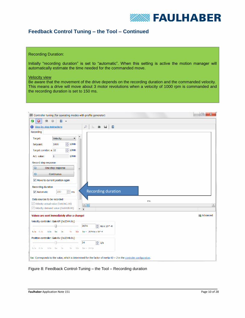
Feedback Control Tuning – the Tool – Continued
Recording Duration: Initially “recording duration” is set to “automatic”. When this setting is active the motion manager will automatically estimate the time needed for the commanded move. Velocity view Be aware that the movement of the drive depends on the recording duration and the commanded velocity. This means a drive will move about 3 motor revolutions when a velocity of 1000 rpm is commanded and the recording duration is set to 150 ms.
Figure 8: Feedback Control-Tuning – the Tool – Recording duration
Recording duration
Faulhaber Application Note 151 Page 11 of 28
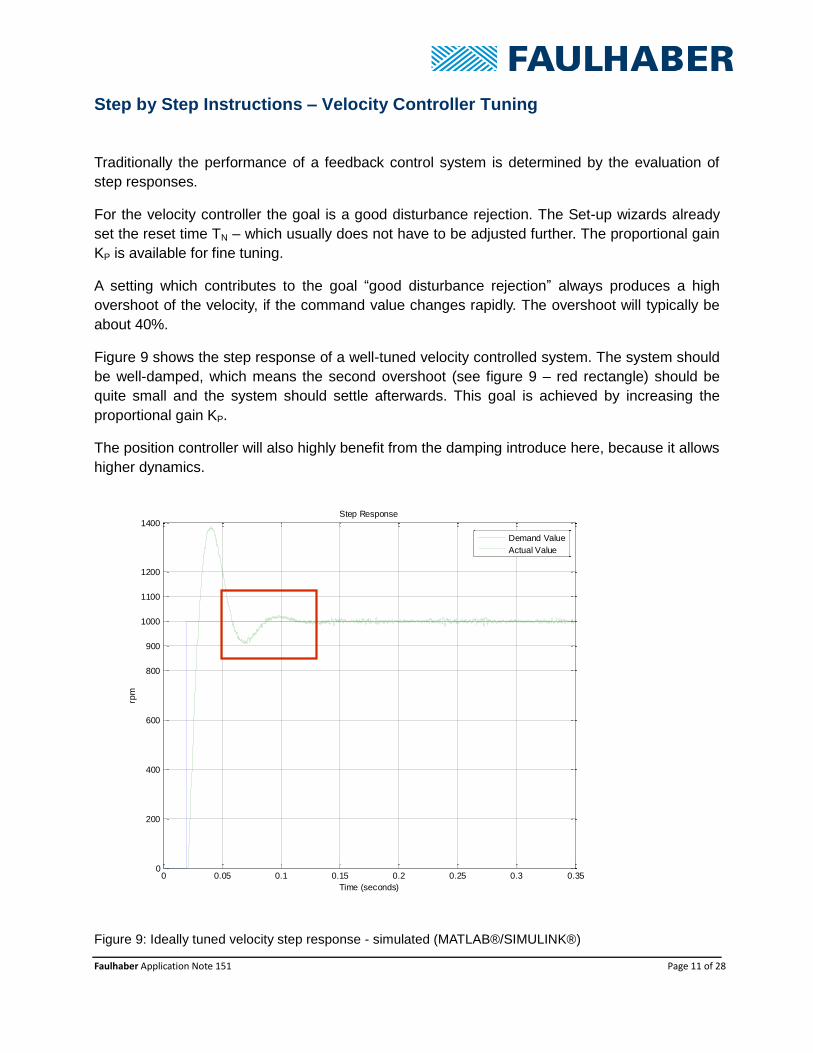
Step by Step Instructions – Velocity Controller Tuning
Traditionally the performance of a feedback control system is determined by the evaluation of
step responses.
For the velocity controller the goal is a good disturbance rejection. The Set-up wizards already
set the reset time TN – which usually does not have to be adjusted further. The proportional gain
KP is available for fine tuning.
A setting which contributes to the goal “good disturbance rejection” always produces a high
overshoot of the velocity, if the command value changes rapidly. The overshoot will typically be
about 40%.
Figure 9 shows the step response of a well-tuned velocity controlled system. The system should
be well-damped, which means the second overshoot (see figure 9 – red rectangle) should be
quite small and the system should settle afterwards. This goal is achieved by increasing the
proportional gain KP.
The position controller will also highly benefit from the damping introduce here, because it allows
higher dynamics.
Figure 9: Ideally tuned velocity step response - simulated (MATLAB®/SIMULINK®)
0 0.05 0.1 0.15 0.2 0.25 0.3 0.350
200
400
600
800
900
1000
1100
1200
1400
Time (seconds)
rpm
Step Response
Demand Value
Actual Value
Faulhaber Application Note 151 Page 12 of 28
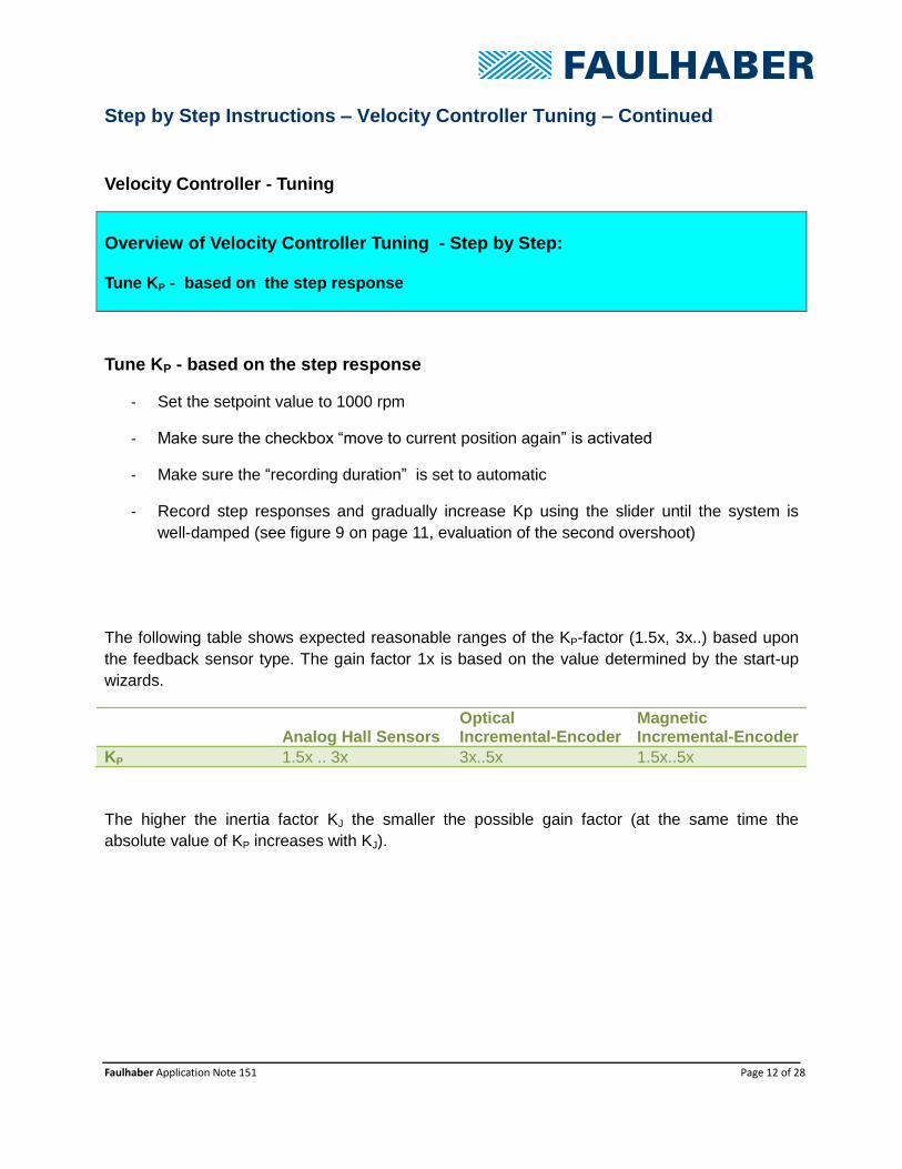
Step by Step Instructions – Velocity Controller Tuning – Continued
Velocity Controller - Tuning
Overview of Velocity Controller Tuning - Step by Step: Tune KP - based on the step response
Tune KP - based on the step response
- Set the setpoint value to 1000 rpm
- Make sure the checkbox “move to current position again” is activated
- Make sure the “recording duration” is set to automatic
- Record step responses and gradually increase Kp using the slider until the system is
well-damped (see figure 9 on page 11, evaluation of the second overshoot)
The following table shows expected reasonable ranges of the KP-factor (1.5x, 3x..) based upon
the feedback sensor type. The gain factor 1x is based on the value determined by the start-up
wizards.
Analog Hall Sensors
Optical Incremental-Encoder
Magnetic Incremental-Encoder
KP 1.5x .. 3x 3x..5x 1.5x..5x
The higher the inertia factor KJ the smaller the possible gain factor (at the same time the
absolute value of KP increases with KJ).
Faulhaber Application Note 151 Page 13 of 28
Step by Step Instructions – Velocity Controller Tuning – Continued
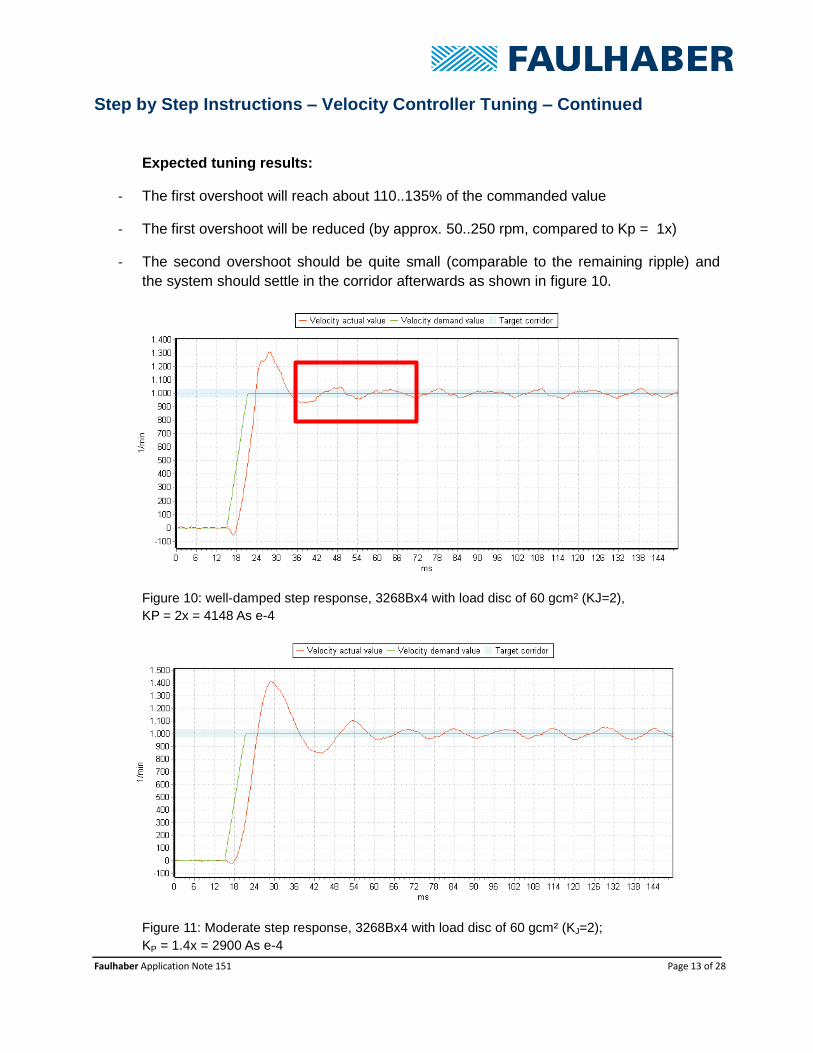
Expected tuning results:
- The first overshoot will reach about 110..135% of the commanded value
- The first overshoot will be reduced (by approx. 50..250 rpm, compared to Kp = 1x)
- The second overshoot should be quite small (comparable to the remaining ripple) and
the system should settle in the corridor afterwards as shown in figure 10.
Figure 10: well-damped step response, 3268Bx4 with load disc of 60 gcm² (KJ=2),
KP = 2x = 4148 As e-4
Figure 11: Moderate step response, 3268Bx4 with load disc of 60 gcm² (KJ=2);
KP = 1.4x = 2900 As e-4
Faulhaber Application Note 151 Page 14 of 28
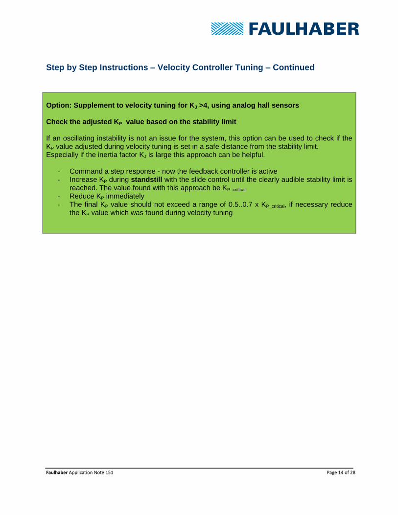
Step by Step Instructions – Velocity Controller Tuning – Continued
Option: Supplement to velocity tuning for KJ >4, using analog hall sensors Check the adjusted KP value based on the stability limit If an oscillating instability is not an issue for the system, this option can be used to check if the KP value adjusted during velocity tuning is set in a safe distance from the stability limit. Especially if the inertia factor KJ is large this approach can be helpful.
- Command a step response - now the feedback controller is active - Increase KP during standstill with the slide control until the clearly audible stability limit is
reached. The value found with this approach be KP_critical - Reduce KP immediately - The final KP value should not exceed a range of 0.5..0.7 x KP_critical, if necessary reduce
the KP value which was found during velocity tuning
Faulhaber Application Note 151 Page 15 of 28
Step by Step Instructions – Position Controller Tuning
As the positon control loop encompasses the velocity control loop (as shown in figure 1), the
positon control loop’s performance ultimately depends upon the performance of the velocity
control loop. In other words, the velocity control loop must be tuned before the position control
loop, if not tuned yet, please go back to page 11.
The desired result of position controller tuning in this application note is a fast response with little to no positional overshoot. The section shows how to use Kv for tuning the Position Control Loop.
Position Controller Tuning
Overview of Position Controller Tuning - Step by Step: Step 1: Adjust Max Motor Speed
Step 2: Tune KV – based on the Step Response - commanding small distances
Step 3: Configure the following error as a quick stop source
Step 4: Check the settings - commanding longer distances
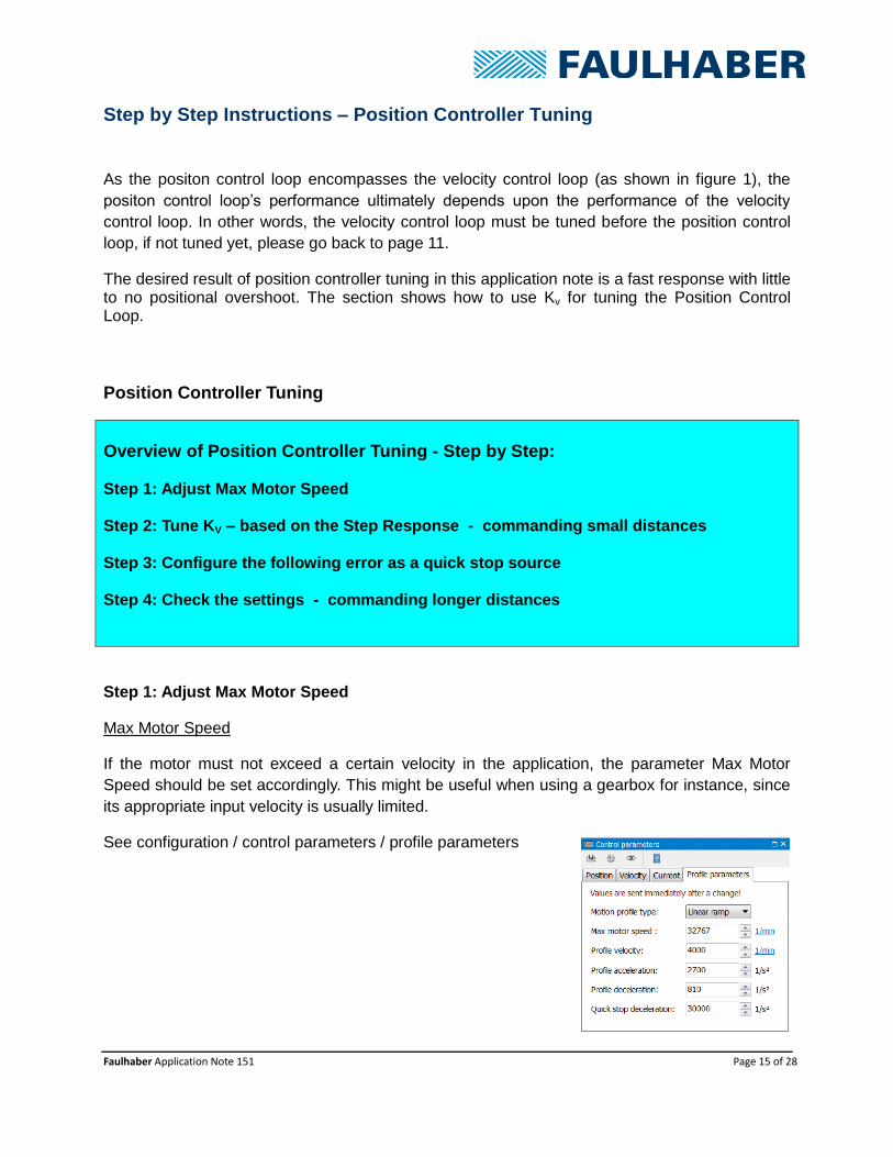
Step 1: Adjust Max Motor Speed
Max Motor Speed
If the motor must not exceed a certain velocity in the application, the parameter Max Motor
Speed should be set accordingly. This might be useful when using a gearbox for instance, since
its appropriate input velocity is usually limited.
See configuration / control parameters / profile parameters

Faulhaber Application Note 151 Page 16 of 28
Step by Step Instructions – Position Controller Tuning – Continued
Step 2: Tune KV – based on the Step Response - using small distances
- Set the setpoint value to ¼ motor revolution (see also page 8)
- Record step responses and gradually increase KV until the desired dynamic is reached
- If the graph of the actual position shows slight oscillations, it is usually not useful to
further increase KV
- If the system shows some oscillation in the final position, KV has to be reduced again
- Save the determined parameter KV “permanently”
The following table shows expected reasonable ranges of the KV-factor value (2x, 5x..) based
upon the feedback sensor type. The gain factor 1x is based on the value determined by the
start-up wizards.
Analog Hall Sensors
Optical Incremental-Encoder
Magnetic Incremental-Encoder
KV 2x .. 5x 5x..10x 2x..10x
Systems that function well on the higher end of the range of the KP-factor (see page 12) will
most likely function well on the higher end of the range of the KV-factor.
Faulhaber Application Note 151 Page 17 of 28
Step by Step Instructions – Position Controller Tuning – Continued
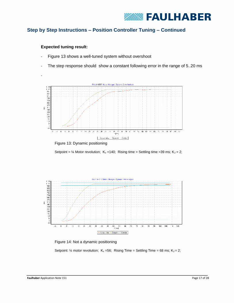
Expected tuning result:
- Figure 13 shows a well-tuned system without overshoot
- The step response should show a constant following error in the range of 5..20 ms
-
Figure 13: Dynamic positioning
Setpoint = ¼ Motor revolution; Kv =140; Rising time = Settling time =39 ms; KJ = 2;
Figure 14: Not a dynamic positioning
Setpoint: ¼ motor revolution; Kv =56; Rising Time = Settling Time = 68 ms; KJ = 2;
Faulhaber Application Note 151 Page 18 of 28
Step by Step Instructions – Position Controller Tuning – Continued
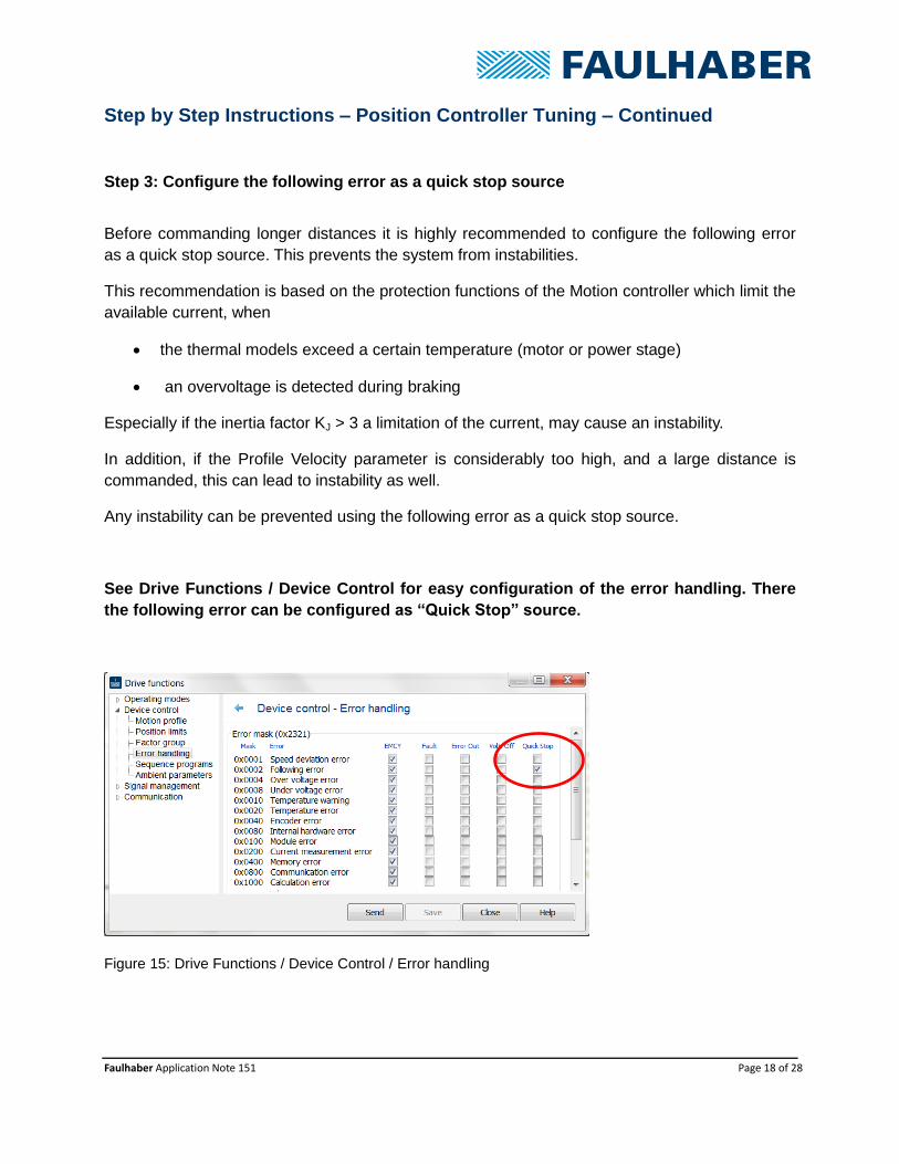
Step 3: Configure the following error as a quick stop source
Before commanding longer distances it is highly recommended to configure the following error
as a quick stop source. This prevents the system from instabilities.
This recommendation is based on the protection functions of the Motion controller which limit the
available current, when
the thermal models exceed a certain temperature (motor or power stage)
an overvoltage is detected during braking
Especially if the inertia factor KJ > 3 a limitation of the current, may cause an instability.
In addition, if the Profile Velocity parameter is considerably too high, and a large distance is
commanded, this can lead to instability as well.
Any instability can be prevented using the following error as a quick stop source.
See Drive Functions / Device Control for easy configuration of the error handling. There
the following error can be configured as “Quick Stop” source.
Figure 15: Drive Functions / Device Control / Error handling
Faulhaber Application Note 151 Page 19 of 28
Step by Step Instructions – Position Controller Tuning – Continued
Step 4: Check the settings - commanding longer distances
- Restart the Tuning Tool
- Set Setpoints relevant for the application (distance wise)
- Modify KV, if necessary
- Modify the Profile Velocity (see “Advanced” settings), if necessary
- Save the determined parameters “permanently”
After following the steps 1..4, the position controller tuning is completed.
Faulhaber Application Note 151 Page 20 of 28
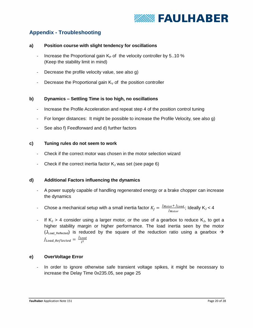
Appendix - Troubleshooting
a) Position course with slight tendency for oscillations
- Increase the Proportional gain KP of the velocity controller by 5..10 %
(Keep the stability limit in mind)
- Decrease the profile velocity value, see also g)
- Decrease the Proportional gain KV of the position controller
b) Dynamics – Settling Time is too high, no oscillations
- Increase the Profile Acceleration and repeat step 4 of the position control tuning
- For longer distances: It might be possible to increase the Profile Velocity, see also g)
- See also f) Feedforward and d) further factors
c) Tuning rules do not seem to work
- Check if the correct motor was chosen in the motor selection wizard
- Check if the correct inertia factor KJ was set (see page 6)
d) Additional Factors influencing the dynamics
- A power supply capable of handling regenerated energy or a brake chopper can increase
the dynamics
- Chose a mechanical setup with a small inertia factor 𝐾𝐽 = 𝐽𝑀𝑜𝑡𝑜𝑟+ 𝐽𝐿𝑜𝑎𝑑
𝐽𝑀𝑜𝑡𝑜𝑟; Ideally KJ < 4
- If KJ > 4 consider using a larger motor, or the use of a gearbox to reduce KJ, to get a
higher stability margin or higher performance. The load inertia seen by the motor
(JLoad_Reflected) is reduced by the square of the reduction ratio using a gearbox
𝐽𝐿𝑜𝑎𝑑_𝑅𝑒𝑓𝑙𝑒𝑐𝑡𝑒𝑑 = 𝐽𝐿𝑜𝑎𝑑
𝑖2
e) OverVoltage Error
- In order to ignore otherwise safe transient voltage spikes, it might be necessary to
increase the Delay Time 0x235.05, see page 25
Faulhaber Application Note 151 Page 21 of 28
Appendix – Expert Tuning
f) Path Accuracy and Dynamics – Feedforward for Position Control
This approach shall increase the path accuracy by using Velocity Feedforward and may further
reduce the settling time:
- First, the Step by Step Tuning starting on page 11, ending on page 19 has to be
performed, especially the Following error has to be configured as quick stop source (see
page 18).
- Only then the Velocity Feed Forward should be activated.
In Position View the Velocity-Feed-Forward-Value should be set to 100 % ( = 128).
Figure 16: Control and Feedforward Parameters
As a result the following error will be reduced. The settling time might be reduced by 1 to 10
ms, depending on how well the system was tuned before.
Velocity Feedforward might cause a tendency for small oscillations before settling. If this is
the case and the tuning goal is to reach the commanded position without any overshoot, it
might be helpful to consider current feedforward in addition - see page 22.
Figure 17: Positioning with Feedforward of Velocity
Velocity feedforward
Advanced
Faulhaber Application Note 151 Page 22 of 28
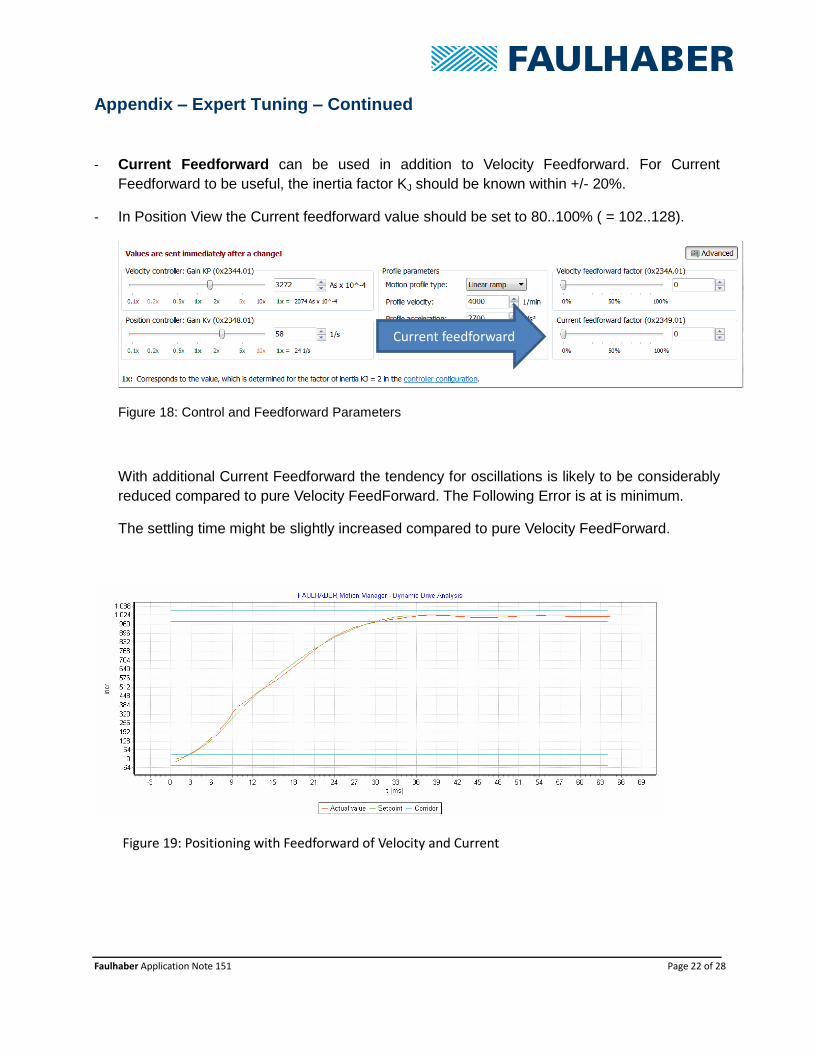
Appendix – Expert Tuning – Continued
- Current Feedforward can be used in addition to Velocity Feedforward. For Current
Feedforward to be useful, the inertia factor KJ should be known within +/- 20%.
- In Position View the Current feedforward value should be set to 80..100% ( = 102..128).
Figure 18: Control and Feedforward Parameters
With additional Current Feedforward the tendency for oscillations is likely to be considerably
reduced compared to pure Velocity FeedForward. The Following Error is at is minimum.
The settling time might be slightly increased compared to pure Velocity FeedForward.
Figure 19: Positioning with Feedforward of Velocity and Current
Current feedforward
Faulhaber Application Note 151 Page 23 of 28
Appendix – Expert Tuning – Continued
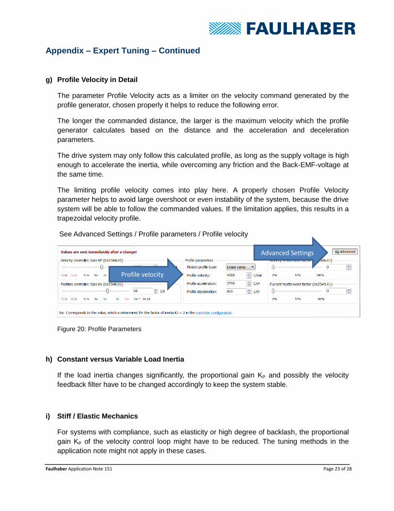
g) Profile Velocity in Detail
The parameter Profile Velocity acts as a limiter on the velocity command generated by the
profile generator, chosen properly it helps to reduce the following error.
The longer the commanded distance, the larger is the maximum velocity which the profile
generator calculates based on the distance and the acceleration and deceleration
parameters.
The drive system may only follow this calculated profile, as long as the supply voltage is high
enough to accelerate the inertia, while overcoming any friction and the Back-EMF-voltage at
the same time.
The limiting profile velocity comes into play here. A properly chosen Profile Velocity
parameter helps to avoid large overshoot or even instability of the system, because the drive
system will be able to follow the commanded values. If the limitation applies, this results in a
trapezoidal velocity profile.
See Advanced Settings / Profile parameters / Profile velocity
Figure 20: Profile Parameters
h) Constant versus Variable Load Inertia
If the load inertia changes significantly, the proportional gain KP and possibly the velocity
feedback filter have to be changed accordingly to keep the system stable.
i) Stiff / Elastic Mechanics
For systems with compliance, such as elasticity or high degree of backlash, the proportional
gain KP of the velocity control loop might have to be reduced. The tuning methods in the
application note might not apply in these cases.
Profile velocity
Advanced Settings

Faulhaber Application Note 151 Page 24 of 28
Faulhaber Application Note 151 Page 25 of 28
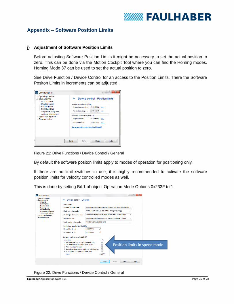
Appendix – Software Position Limits
j) Adjustment of Software Position Limits
Before adjusting Software Position Limits it might be necessary to set the actual position to
zero. This can be done via the Motion Cockpit Tool where you can find the Homing modes.
Homing Mode 37 can be used to set the actual position to zero.
See Drive Function / Device Control for an access to the Position Limits. There the Software
Positon Limits in increments can be adjusted.
Figure 21: Drive Functions / Device Control / General
By default the software positon limits apply to modes of operation for positioning only.
If there are no limit switches in use, it is highly recommended to activate the software
position limits for velocity controlled modes as well.
This is done by setting Bit 1 of object Operation Mode Options 0x233F to 1.
Figure 22: Drive Functions / Device Control / General
Position limits in speed mode
Faulhaber Application Note 151 Page 26 of 28
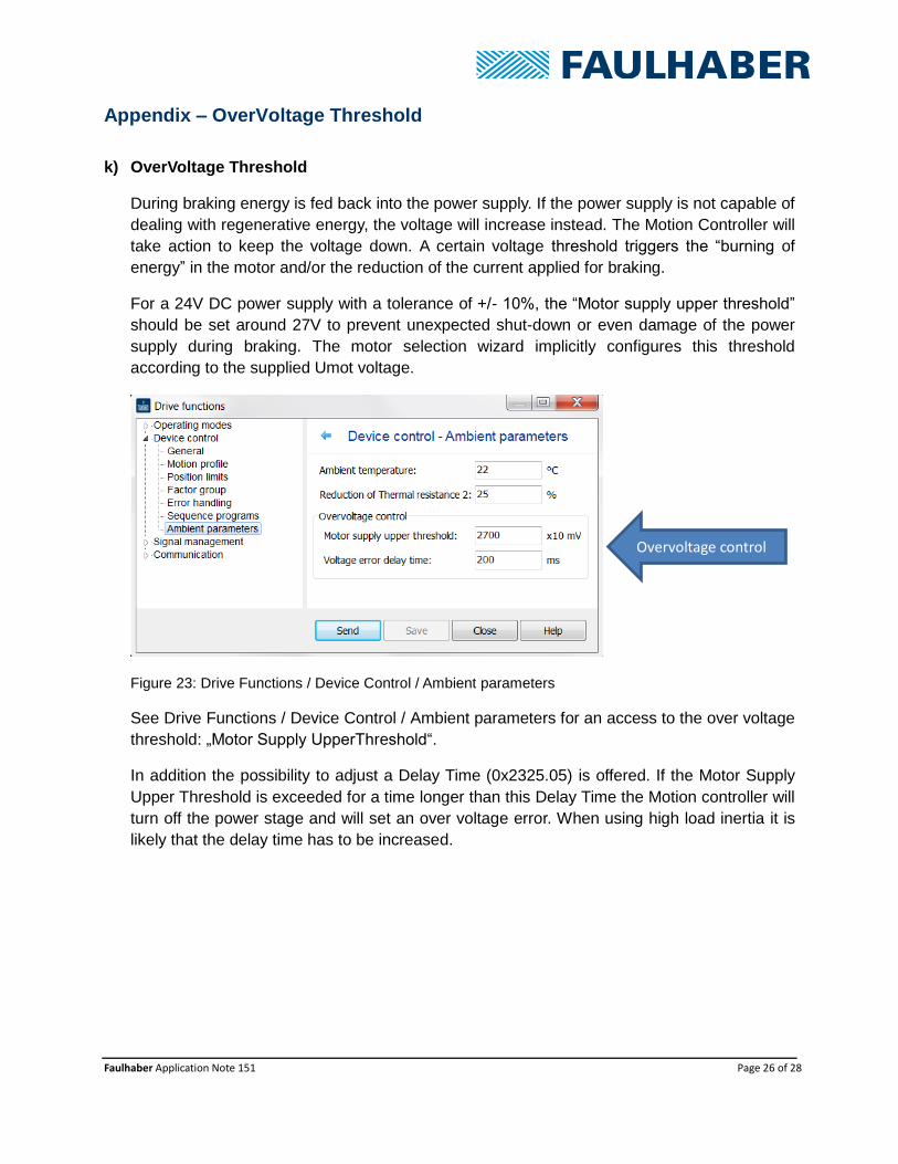
Appendix – OverVoltage Threshold
k) OverVoltage Threshold
During braking energy is fed back into the power supply. If the power supply is not capable of
dealing with regenerative energy, the voltage will increase instead. The Motion Controller will
take action to keep the voltage down. A certain voltage threshold triggers the “burning of
energy” in the motor and/or the reduction of the current applied for braking.
For a 24V DC power supply with a tolerance of +/- 10%, the “Motor supply upper threshold”
should be set around 27V to prevent unexpected shut-down or even damage of the power
supply during braking. The motor selection wizard implicitly configures this threshold
according to the supplied Umot voltage.
Figure 23: Drive Functions / Device Control / Ambient parameters
See Drive Functions / Device Control / Ambient parameters for an access to the over voltage
threshold: „Motor Supply UpperThreshold“.
In addition the possibility to adjust a Delay Time (0x2325.05) is offered. If the Motor Supply
Upper Threshold is exceeded for a time longer than this Delay Time the Motion controller will
turn off the power stage and will set an over voltage error. When using high load inertia it is
likely that the delay time has to be increased.
Overvoltage control
Faulhaber Application Note 151 Page 27 of 28
Appendix – Non-Profile Modes of Operation
l) Usage of Non-Profile Modes of Operation
- Cyclic Modes:
By design cyclic modes depend on a stream of command values (and maybe additional
feedforward values) from a Master PLC at regular intervals in the range of typically 1 to
10 ms. The control system can be tuned using the tuning tool, but afterwards the profile
parameters have to be transferred to the Master PLC for the calculation of the command
trajectory.
- Analog Modes:
Analog Modes do not make use of the profile generator either. Instead command filters
have to be used. If the Motion Manager Tool shall be used for control tuning, the
maximum profile parameter values should be set and a command filter has to be
activated.
Faulhaber Application Note 151 Page 28 of 28
Rechtliche Hinweise
Urheberrechte. Alle Rechte vorbehalten. Ohne vorherige ausdrückliche schriftliche Genehmigung der Dr.
Fritz Faulhaber & Co. KG darf insbesondere kein Teil dieser Application Note vervielfältigt, reproduziert, in
einem Informationssystem gespeichert oder be- oder verarbeitet werden.
Gewerbliche Schutzrechte. Mit der Veröffentlichung der Application Note werden weder ausdrücklich
noch konkludent Rechte an gewerblichen Schutzrechten, die mittelbar oder unmittelbar den beschriebe-
nen Anwendungen und Funktionen der Application Note zugrunde liegen, übertragen noch Nutzungsrech-
te daran eingeräumt.
Kein Vertragsbestandteil; Unverbindlichkeit der Application Note. Die Application Note ist nicht Ver-
tragsbestandteil von Verträgen, die die Dr. Fritz Faulhaber GmbH & Co. KG abschließt, soweit sich aus
solchen Verträgen nicht etwas anderes ergibt. Die Application Note beschreibt unverbindlich ein mögli-
ches Anwendungsbeispiel. Die Dr. Fritz Faulhaber GmbH & Co. KG übernimmt insbesondere keine Ga-
rantie dafür und steht insbesondere nicht dafür ein, dass die in der Application Note illustrierten Abläufe
und Funktionen stets wie beschrieben aus- und durchgeführt werden können und dass die in der Applica-
tion Note beschriebenen Abläufe und Funktionen in anderen Zusammenhängen und Umgebungen ohne
zusätzliche Tests oder Modifikationen mit demselben Ergebnis umgesetzt werden können.
Keine Haftung. Die Dr. Fritz Faulhaber GmbH & Co. KG weist darauf hin, dass aufgrund der Unverbind-
lichkeit der Application Note keine Haftung für Schäden übernommen wird, die auf die Application Note
zurückgehen.
Änderungen der Application Note. Änderungen der Application Note sind vorbehalten. Die jeweils aktu-
elle Version dieser Application Note erhalten Sie von Dr. Fritz Faulhaber GmbH & Co. KG unter der Tele-
fonnummer +49 7031 638 688 oder per Mail von [email protected].
Legal notices
Copyrights. All rights reserved. No part of this Application Note may be copied, reproduced, saved in an
information system, altered or processed in any way without the express prior written consent of Dr. Fritz
Faulhaber & Co. KG.
Industrial property rights. In publishing the Application Note Dr. Fritz Faulhaber & Co. KG does not ex-
pressly or implicitly grant any rights in industrial property rights on which the applications and functions of
the Application Note described are directly or indirectly based nor does it transfer rights of use in such
industrial property rights.
No part of contract; non-binding character of the Application Note. Unless otherwise stated the Ap-
plication Note is not a constituent part of contracts concluded by Dr. Fritz Faulhaber & Co. KG. The Appli-
cation Note is a non-binding description of a possible application. In particular Dr. Fritz Faulhaber & Co.
KG does not guarantee and makes no representation that the processes and functions illustrated in the
Application Note can always be executed and implemented as described and that they can be used in
other contexts and environments with the same result without additional tests or modifications.
No liability. Owing to the non-binding character of the Application Note Dr. Fritz Faulhaber & Co. KG will
not accept any liability for losses arising in connection with it.
Amendments to the Application Note. Dr. Fritz Faulhaber & Co. KG reserves the right to amend Appli-
cation Notes. The current version of this Application Note may be obtained from Dr. Fritz Faulhaber & Co.
KG by calling +49 7031 638 688 or sending an e-mail to [email protected].