application of bayesian decision theory based on prior

Application of Bayesian Decision Theory Based on Prior Information in the Multi-Objective Optimization Problem

Xia Lei National Key Laboratory of Communications, University of Electronic Science and Technology of China

Chengdu, 610065, P.R. China E-mail: [email protected]

Maozhu Jin*Business School of Sichuan University

Chengdu, 610065, P.R. China E-mail: [email protected]

Qiang Wang National Key Laboratory of Communications, University of Electronic Science and Technology of China

Chengdu, 610065, P.R. China E-mail: wangqiang @uestc.edu.cn

Abstract

General multi-objective optimization methods are hard to obtain prior information, how to utilize prior information has been a challenge. This paper analyzes the characteristics of Bayesian decision-making based on maximum entropy principle and prior information, especially in case that how to effectively improve decision-making reliability in deficiency of reference samples. The paper exhibits effectiveness of the proposed method using the real application of multi-frequency offset estimation in distributed multiple-input multiple-output system. The simulation results demonstrate Bayesian decision-making based on prior information has better global searching capability when sampling data is deficient.

Keywords: Multi-Objective Optimization, Prior Information, Maximum Entropy Principle, Distributed multiple inputs and multiple outputs.

1. Introduction

Bayesian statistics is one of key branches in modern statistics has its origin of the famous paper ‘Discussion on the Problem of Problem of a Chance or an Opportunity’ authored by British scholar Thomas Bayes (1702-1761) which proposed the Bayesian formulation and the corresponding reasoning method. The basic point of view in Bayesian statistics study is that any unknown parameter should be regarded as a statistics variable which can be described by a

probability distribution, a prior distribution which represents the knowledge of the event before proceeding sampling investigation.1-3 This is what the difference lies between Bayesian statistics and classic statistics. Classic statistic scholars didn’t recognize the prior information and advocates the statistical deduce using sample information, but that situation has changed and prior information has gained acknowledge in classic statistics. The focal argument is how to obtain and utilize the prior information to determine the prior distribution appropriately.

---------------------------------------* Corresponding author

International Journal of Computational Intelligence Systems, Suppl. 1 (December, 2010).

Published by Atlantis Press Copyright: the authors 31

X. Lei et al

Bayesian decision obtains the conditional distribution density (prior distribution) of unknown parameters in condition of known sampling distribution. Since this sampling distribution is obtained after the sampling process is complete, it is called posteriori distribution. The key to Bayesian deduction is that any results must and can only rely on posteriori distribution. Multi-objective decision-making method focuses on simultaneous optimization of multiple targets, different targets can’t use uniform measuring criteria and more usually than not these targets are contradictory.3 So in this sense multi-objective decision-making gives rise to a set of trade-off optimal solutions, instead of a single optimum solution.4

From Bayesian statistics perspective, Bayesian multi-objective decision-making deals with the multi-risk problem using multi-objective decision-making principles. Bayesian decision-making which falls into the conventional decision-making field focuses on single objective decision. However, multi-objective decision-making theory has neglected the benefits of Bayesian decision-making to handle multi-objective decision-making problem with uncertainties.5,6

Bayesian decision-making estimates probabilities of partly unknown parameters and rectify the probability using Bayesian formula, and in last step, making decision according to the expectation value and rectified probabilities.7 Suppose that θ is the objective parameter, then the optimization proceeds using maximum posteriori distribution based on Bayesian Criterions, which makes

( )ˆ arg max xpθ

θ θ= (1)

Where is the data vector including the information of xθ . To get maximum value of ( xp θ ) , we observe

( ) ( ) ( )( )

xx

xp p

ppθ θ

θ = (2)

So maximum value of ( ) ( )xp pθ θ is equivalent to (1). According to (2), other than the existence of prior probability density function (PDF), ( ) ( )xp pθ θ is tantamount to maximum likelihood examination. Therefore,

( ) ( )ˆ arg max xp pθ

θ θ θ= (3)

Or

( ) ( )ˆ arg max ln lnxp pθ

θ θ θ⎡ ⎤= +⎣ ⎦ (4)

The PDF of prior information is more “abrupt”, more important influence it will put on the estimation. Information is more included on the sampling data, more effects sampling data will exert on the estimation, at the same time the influence of prior information will wane. ,8 9

Put it in another way, when information provided by sampling data is deficient, the performance of optimization strategy will be compromised. Making appropriate use of prior information to make up for this deficiency is of great importance to improve the effect of strategic optimization.10,11

Previous study based on Bayesian Criterions deals with the situation that Bayesian Criterions is relevant to prior probability and cost function when prior probability and cost function are known. But in a real setting, prior probability and cost function may stay unknown and fuzzy; in that case, how they take effect on the system performance remains a challenge to the academia worthy of further research.12

2. System Model

Distributed multiple inputs and multiple outputs (MIMO) system is an important application area of future communication technique. It uses multiple parallel channels transmission method so that it can achieve higher transmission efficiency. After applied the distributed antenna configuration, the original single-objective optimization problem become a typical multi-objective optimization problem because transmitting antennas or receiving antennas located in different geographic locations and using different crystal lead to different transmitting antennas to the same receiving antennas has different frequency offset. Even a general distributed MIMO system that transmitting antenna located in a different location, the mobile service also uses a distributed antenna. At this point, we could consider that the time delay and frequency offset between different receiving antenna and transmitting antenna will different too. Under such assumptions, the time matrix offset and frequency offset matrix could extended to


Prior Information In Optimization

(5)

1,1 1,2 1,

2,1 2,2 2,,

,1 ,2 ,

Θ

T

T

R R R T

M

Mi j

M M M M

θ θ θ

θ θ θθ

θ θ θ

⎡⎢⎢ ⎥⎡ ⎤= =⎣ ⎦ ⎢⎢⎢⎣

…

…

⎤⎥

⎥⎥⎥⎦

⎤⎥⎥ (6)

1,1 1,2 1,

2,1 2,2 2,,

,1 ,2 ,

E

T

T

R R R T

M

Mi j

M M M M

ε ε ε

ε ε εε

ε ε ε

⎡⎢⎢⎡ ⎤= =⎣ ⎦ ⎢ ⎥⎢ ⎥⎢ ⎥⎣ ⎦

…

…

Where, ,i jθ

denotes time offset between receiving

antenna i and receiving antenna j, ,i jε denotes normalized frequency offset between receiving antenna i and receiving antenna j. (6) indicates when both transmitting antennas and receiving antennas employ distributed model, frequency offset estimation is transformed into the problem of multi-parameter estimation. Analysis on maximum posteriori estimation has inspired us to utilize prior information of frequency offset to estimate multi-frequency offset in distributed MIMO system. Especially in the environment of low signal-noise-ratio (SNR), analysis on maximum posteriori estimation of multi-frequency offset has great applicable value on improving the performance of frequency synchronization. Considering the case of distributed MIMO system with TM transmitting antennas and RM receiving antennas, which is tantamount to RM distributed multi-input single-output (MISO) systems. Without loss of generality, this paper focuses on the kth MISO system, the receiving signal can be represented by

(7) 1

1y E X ω

TMN

k l l ll

h ×

=

= + ∈∑ C

1,2, , Tk ∈ Elwhere , is diagonal matrix with elements of

{ }M

[ ] 2,

E lj nl n n

e πε= (8)

lε is the frequency offset produced by lth transmitting antenna. is the sequence send by l1X N

l C ×∈ th transmitting antenna and is flat fading channel coefficient. is complex Gaussian noise vector.

{ }, 1, 2, ,l Th l M∈( 2,ω 0 ICN σ∈

2.1. Obtaining strategy of prior information based on the principle of maximum entropy

According to the description of the previous section, prior information in Bayesian decision played an important role, especially when the sample collection of event is inadequate, the prior information could reflect its effect on decision-making optimization. Assuming the probability of discrete random variable x is

( ) , 1, ,i ip x a p i N= = = (9)

when its value equal to , 1, , Na a

( )1

lnN

ii

iH x p=

= −∑ p (10)

Represents the entropy of x , similarly, if x is a continuous random variable, its probability density function is ( )p x , and

( ) ( ) ( )lnH x p x p x= −∫ dx (11)

(11) is finite integrable, similarly, it represents the entropy of x . According to the definition, the entropy only link with random variable’s probability density function, which means related to the distribution of random variables. In 1957, Jaynes ET Jaynes first proposed the maximum entropy principle: among all the compatible distributions, choose some distributions which can make the information entropy reach to its maximum under the situation that suffices some constraint conditions. In case of part of information has gained, therefore, deduction of distribution can be made only if it takes the probability distribution conform to constraints but entropy has the maximum values. Any other options means we add some other constraints or conditions which are unavailable based on the information has already gained. Maximum entropy principle13 is that when priori information distribution is not determined the selected priori information should have maximums entropy distribution. Accordingly, Johnny pointed out that some important real-world probability distributions which comply with the maximums entropy principle under some constraints. When the value of random variable is continuous, meanwhile, if the expectation and variance are known, the maximum entropy distribution is the normal distribution. This paper will prove the results that the

)


X. Lei et al

maximum entropy distribution is Gaussian distribution as random variables’ mean and variance are known. First, there are two lemmas.13

Lemma 1: Suppose is a convex function that the domain is (a, b), which is accountable for random variables

( )tϕ

ξ , ( )Eϕ ξ , (E )ϕ ξ , then

( ) ( )E Eϕ ξ ϕ ξ≥ (12)

Obviously, if

( ) lnt tϕ = t

t

t

))E

(13)

We can get

( ) 1 lntϕ′ = + (14)

( ) 1/tϕ′′ = (15)

hence, is a convex function when , then, ( )tϕ (0,t∈ +∞

( ) ( ) (ln lnE Eξ ξ ξ≥ ξ (16)

can be deduced by(12). Lemma 2: For the distribution probability density function

( ) , 1,2if x i = (17)

if both ends of (18) have meanings, then, (19)is available

( ) ( ) ( ) ( )1 1 1 2ln lnf x f x dx f x f x≥∫ ∫ (20)

Proof: Let

( ) ( ) ( )1 2 2/ ,f f fζ λ λ λ= x∈ (21)

Because

( ) ( )( )( ) ( )

1 2

12

2

/

1

E E f f

ff d

f

ζ λ λ

λλ λ

λ

= ⎡ ⎤⎣ ⎦

=

=

∫ (22)

Then

( )ln 0Eζ = (23)

According to Lemma 1, we can proof

( )( )

( )( ) ( )

( ) ( ) ( ) ( )

1 12

2 2

1 1 1 2

0 ln

ln

ln ln

E

f ff d

f f

f f d f f d

ζ ζ

λ λλ λ

λ λ

λ λ λ λ λ λ

≤

⎛ ⎞= ⎜ ⎟⎜ ⎟

⎝ ⎠

= −

∫

∫ ∫

(24)

Based on Lemma 2, if a random variable’s mean and variance are limited, then the maximal entropy distribution is the Gaussian distribution. Proof: Consider set

( ) ( )

( )

( )2 2

: 0,

0,

p p

P p d

p d ε

ε ε

ε ε ε

ε ε ε σ

+∞

−∞

+∞

−∞

⎧ ⎫≥⎪ ⎪⎪ ⎪= =⎨ ⎬⎪ ⎪⎪ ⎪=⎩ ⎭

∫∫

(25)

Obviously, the probability density function of ( )20,N εε σ∈ is

( ) 2 2/2 20 / 2p e εε σ

εε π− Pσ= ∈ (26)

According to Lemma 2, ( )1p ε P∀ ∈ , then

( ) ( ) ( ) ( )1 1 1 0ln ln 0p p d p p dε ε ε ε ε ε+∞ +∞

−∞ −∞− ≥∫ ∫

(27)

Further deduction of (27), then

( ) ( )

( )

( ) ( )

1 1

21 22

0 02

ln

1 1 ln22

1 1 = ln ln22

p p d

p d

p p

εε

ε

ε ε ε

ε εσπσ

d

ε

ε ε επσ

+∞

−∞

+∞

−∞

+∞

−∞

≥

⎡ ⎤⎢ ⎥−⎢ ⎥⎣ ⎦

− =

∫

∫

∫ (28)

Therefore, the mean 0 and variance of random variables, the maximum entropy distribution is normal distribution. The usual frequency offset estimation is doesn’t consider to use the frequency offset prior information, so the maximum likelihood (ML) estimation method is the most optimal detection algorithm. As previously discussed, the actual frequency offset can be changed as the temperature, humidity and other environmental factors’ change, the Refs. 14 regards the frequency offset as random variables to study the synchronization problem. If you can get frequency offset prior information reasonably, then, it will play an important



role for improving the frequency synchronization under low SNR environment. Refs. 15 proposed a synchronization algorithm in cooperative communication system which based on frequency offset prior information. In low SNR region, it can improve the performance of frequency synchronization. Although the literature proposed the application of frequency offset prior information in collaborative communication environment, however, how to choose the distribution of prior information and obtain the deviation of the prior information and practicing it in a multi-frequency offset estimation of distributed MIMO systems is still a valuable researching direction. Can be realizable in the physical system, frequency offset is often distributed in a limited range, namely ( , )ε η η∈ − . The former literature regards frequency offset as random variables which mean is 0 and variance is 2

εσ . Based on this and combined with the analysis of prior information above, according to the principle of maximum entropy, furthermore, this paper argue that frequency offset obeys normal distribution, ie:

， . ( )20,kk ε

After determining the prior information, the question how to get more reasonable values for the variance parameters is worthy of further study.

Nε σ∈ 1, 2, , Tk M=

According to the Three times standard deviation principle16

{ } ( )3 2 3 1 0.9974P ξξ μ σ− < = Φ − ≈

(29)

As a results, the vast majority of Random variable’s sample will distribute in ( )3 , 3ξ ξμ σ μ σ− + , As for the other areas, we can regard as small probability event, therefore, prior information’s variance can be determined by the Three times standard deviation principle. If frequency offsets’ maximums can be get, , then ( ), , 1, 2, ,k k k k Mε η η∈ − = T

2 2 / 9k kεσ η= (30)

According to the Three times standard deviation principle, using frequency offsets distribution range to do estimation for frequency offsets prior variance in distribution MIMO system is a reasonable method.

2.2. Bayesian decision algorithm based on prior information

The current frequency offset estimation algorithms basically regarded frequency offset as a fixed parameter, however, the facts it becomes a random variable because of the influence of environmental change factors such as temperature, humidity etc is often overlooked. A few literatures (Refs. 14, 15 and 17) had begun to research multi-frequency offset estimation algorithm as the frequency offset change to variable. If prior information of frequency offset can be gained reasonably, it will improve the frequency synchronization performance, especially when sampling data is deficient. Main research of this paper is distributed MIMO system’s maximum posteriori multi-frequency estimation algorithm based on frequency offset priori information.

2.2.1 Optimal Maximum a Posteriori Algorithm

According to Eq.(3), maximum multi-frequency offset estimation of distributed MIMO system is to obtain18

( ) ( )ˆ arg maxε

ε y ε εp p= (31)

Where, ( )y εp is conditional distribution density of received sampling data and is distribution density of prior information, they are respectively

( )εp

( )2

2 21

1 1expy ε y E XTM

l l lN Nl

p hπ σ σ =

⎧ ⎫⎪ ⎪= −⎨ ⎬⎪ ⎪⎩ ⎭

∑ (32)

( )( ) ( )

112

1 1exp2

2 detε ε R ε

R

T

Np

π

−⎧ ⎫= ⎨ ⎬⎩ ⎭

(33)

Taking the logarithm of objective function ( ) ( )y ε εp p

( ) ( ) ( )

21

21

, ln ln

1 1 2

y ε y ε ε

y E X ε R εTM

Tl l l

l

L p p

hσ

−

=

= + ∝

− − −∑(34)

Note

1 1 2 2, , ,Z E X E X E XT TM M⎡ ⎤= ⎣ ⎦ (35)

and estimate maximum likelihood (ML) of channel in case of known frequency offset

2ˆ minH

H y ZH= − (36)


X. Lei et al

Further simplify and get

(37) ( ) 1H Z Z Z yH H∧ −=

Substitute (37) into (34) and simplify the result to get

( ) 2 12

1 1,2

y ε y ZH ε R εTLσ

−∝ − − − (38)

With the Eq.(31), then MAP estimation of multi-frequency offset is obtain by

( )( )221 1

ˆ

arg min2ε

ε

I Z Z Z Z y ε R εH H Tσ− −

=

⎧ ⎫− +⎨ ⎬

⎩ ⎭

(39)

(39) indicates the first term of objective function is maximum likelihood estimation and second term is produced by prior information. When prior information is not considered, objective function is converted to ML estimation

( )( ) 21ˆ arg min

εε I Z Z Z Z yH H

ML

−⎧ ⎫= −⎨ ⎬

⎩ ⎭(40)

In essence (40) is same as ML estimation, that is equivalent to

( ) 1ˆ arg max

εε y Z Z Z Z yH H H

ML

−= (41)

It is evident that maximum a posteriori (MAP) estimation of multi-frequency offset combines sampling information of receiving data and prior information of frequency offset. The general ML estimation can only be based on data sampling information, so if interference is relative large (for example, low SNR) or training sequence is short, received signal sample can’t provide sufficient useful information that results in worse performance of frequency offset estimation. MAP estimation introducing prior information combines information of data sample and prior information of frequency offset to make up the deficiency of insufficient useful information of data sample.

2.2.2 Suboptimum Quasi Maximum a Posteriori algorithm

Analysis in section 2.2.1 obtains objective function of multi-frequency offset MAP estimation and indicates there is internal correlation between MAP estimation and ML estimation. So borrowing from the insights of

ML estimation algorithm (for example, Expectation Conditional Maximum (ECM) algorithm) MAP estimation based on prior information can be obtained, but complexity will increase in direct solving objective function due to introduction of prior information. Next, the paper will propose a suboptimum MAP estimation algorithm, that is, quasi maximum a posteriori (QMAP) algorithm. Since ML estimation is an unbiased estimation,

ˆ( ) ,1,2, ,l lE TMε ε= (42)

The mean square error can be represented by

(43) ( ) ( )2ˆ ˆl l lMSE Eε ε ε⎡= −⎣⎤⎦

Eq. (43) is equivalent to

( ) ( )( ) ( )( )( )2ˆ ˆ ˆ ˆl l l l lMSE E E Eε ε ε ε ε⎡ ⎤= − + −⎢ ⎥⎣ ⎦

(44)

Simplify Eq.(44) and get

(45) ( ) ( ) ( )( )2ˆ ˆ ˆvarl l l lMSE E Eε ε ε ε⎡ ⎤= + −⎣ ⎦

Where ( )ˆvar lε is variance of the estimator l̂ε . According to the analysis, theoretically MAP estimation will get better estimation performance, which is smaller MSE. Suppose that MAP estimation is19

,l̂ MAP l l̂ε α ε= (46)

and substitute this estimator into (45), that will make MSE smaller, that is

( ) ( ) ( )( )2,ˆ ˆ ˆvarl MAP l l l l lMSE E Eε α ε α ε⎡ ⎤= + −

⎣ ⎦ε (47)

Simplify Eq.(47) and get

( ) ( ) ( )22,ˆ ˆvarl MAP l l l l lMSE Eε α ε α ε ε⎡ ⎤= + −⎣ ⎦ (48)

Doing the derivation over parameter lα in (48) and set the results equal to zero

( ) ( ) ( ) ( )2,ˆ ˆ2 var 2 1

0

l MAP l l l ll

MSE E ˆε α ε α εα∂

= + −∂

= (49)

Then, we can get the lα that can satisfy the condition



( )

( ) ( )

2

2

ˆ

ˆ ˆvarl

ll l

E

E

εα

ε ε=

+ (50)

Combining the statistical characteristics of prior information, when SNR gradually increases,

ll( )2ˆ 2E εε σ→ and at the same time ( )ˆvar lε will gradually approach cramer–rao low bound (CRLB). However, exact CRLB of ML estimation is dependent on information channel and frequency offset. If ( )ˆvar lε is substituted by approaching CRLB, this will produce result that it is only related to power of training sequence

( )2

2 33

6 6l̂

ll l

asCRLBN P SNRN P h

σε = ∝i ii i

(51)

Where

( ){ }2, 1,2, ,lP E x l l N= = (52)

According to this, the paper gets the approximate corrected value

( )

2

2 ˆl

l

llasCRLB

ε

ε

σα

σ ε=

+ (53)

In summary, ML estimator of frequency offset can be obtained by only using information of the data sample. So when prior information is taken into consideration, approximate estimator of MAP can be obtained by multiplying corrected value calculated by Eq. (53) with ML estimator and the result doesn’t introduce extra complexity.

3. Simulation Results and Analysis

Fig.1 provides low limit performance curve of frequency estimation based on maximum likelihood and maximum posterior principle. Assuming that average value of frequency offset is zero, variance of frequency offset is decided by hardware characteristics of crystal oscillator. According to recent study, variance of frequency offset can be estimated by certain algorithms. Suppose that instability of crystal oscillator with exact estimation will cause standard deviation of prior distribution of frequency offset 0.01εσ =Relevant simulation parameters are listed in table1. 10000 Monte-Carlo simulation tests proceed at each SNR situation.

Table 1.Simulation condition for CRLB based on maximum likelihood and maximum posterior principle

System includes 4 transmitting antennas and 2 receiving antennas

Normalized frequency offset value between Transmitting antenna 1 and

Receiving antennas 1 2 0.01π ⋅


Receiving antenna 1 2 0.015π ⋅





System includes 4 transmitting antennas and 2 receiving antennas


Receiving antennas 1 2 0.01π ⋅



Fig1 indicates when the SNR is low and with known prior information, CRLB of multi-frequency estimation based on maximum posterior estimation is better than that based on maximum likelihood estimation, which provides theoretical basis for frequency estimation using prior information. Then, the paper will provide the simulation results and analysis and makes comparison between two maximum posterior multi-frequency offset algorithms in distributed MIMO systems in the following. Specifically, the paper will explore mean square error performance of optimum MAP estimation and suboptimum QMAP estimation and improvement of frequency synchronization performance in the low SNR environment through Monte-Carlo simulation tests and theoretical analysis. Prior distribution of frequency offset is Gaussian distribution with average value of zero and variance of frequency offset is obtained by estimation of distribution range ( ),η η− .


X. Lei et al

Fig.1. CRLB based on ML and MAP

3.1. Optimal Maximum a Posteriori Algorithm

Here, the paper will make comparison between MAP estimation algorithm and ML estimation algorithm in

and distributed MISO systems and analyze relevant CRLB. To ML estimation, the paper still choose expectation maximum algorithm to get the solution

2 1× 4 1×

20, specific simulation condition is listed in table2.

Table 2. Simulation condition of MAP estimation algorithm

Parameters Distributed

MISO

2 1×

Distributed MISO

4 1×

Length of orthogonal training sequence 32N = 32N =

Range of normalized frequency offset（1） ( )2 0.05,0.05π −i ( )2 0.05,0.05π −i

Range of normalized frequency offset（2） ( )2 0.1,0.1π −i ( )2 0.1,0.1π −i

Information channel flat Rayleigh fading

flat Rayleigh fading

Number of simulation 10000 10000

Due to introduction of prior information of frequency offset, the performance of ML estimation is worse below 0dB. There are two reasons for this: • Algorithm of ML estimation is sensitive at low

SNR and induces the problem of convergence.

• Considering prior information, the frequency offset is no longer set value in conventional estimation, so performance of ML estimation will become worse in strong noise environment.

Fig2 and Fig3 indicates the pperformance comparison in 2 1× distributed MISO system Fig4 and Fig5 indicates the pperformance comparison in 4 1× distributed MISO system

Fig.2.Performance comparison between MAP and ML in 2 1× system ( 0.05η = )




15-5 0 5 1010-5

10-4

10-3

10-2

10-1

100

SNR (dB)

MLMAP

ML — CRLBMAP— CRLB

MSE


Fig.5.Performance comparison between MAP and ML in 4 1×

system ( 0.1η = )

To MAP estimation, in different frequency offset range and and distributed MISO systems, the performance stays stable.

2 1× 4 1×

At , in 2 distributed MISO system, MAP estimation obtains performance gain 5dB more than that of ML estimation; in 4 distributed MISO system, MAP estimation obtains performance gain 5dB smaller than that of ML estimation. This difference results from multi-antenna interference.

5SNR dB= − 1×

1×

When entering the area of , performance of ML and MAP is approaching the same. This is mainly because diminish of noise interference makes enhanced the effective information of sampling data, the effect of prior information is waning, PDF function of sampling

data becomes acute and influence of local convergence is decreasing.

5SNR dB>

Simulation results indicate MAP estimation significantly improves performance frequency synchronization in low environment. Besides, from Fig.2 to Fig.5, it can be observed that CRLB of MAP estimation based on prior information is a little bit lower than that of ML estimation, and they are approaching the same. This observation is consistent with the rules of real estimation performance. Since length of training sequence is 32, ideally information provided by sample data is dominant which results insignificant difference between two methods. It is worth mentioning that range of frequency offset is smaller, so is variance. So prior information play bigger role that cause better performance, otherwise, performance becomes worse.

3.2. Suboptimum Quasi Maximum a Posteriori algorithm

In previous simulation, relatively longer sequence is employed. Here, the paper will use shorter sequence to make comparison between optimum MAP estimation algorithm and suboptimum QMAP estimation algorithm and meanwhile further demonstrate the influence of number of sample data to CRLB. Due to previous mentioned different range of frequency offset, here, only one range of frequency offset is adopted. Relevant simulation parameters are listed in table3.

Table 3. Simulation condition of MAP estimation algorithm

Parameters Distributed

MISO

2 1×

Distributed MISO

4 1×

Length of orthogonal training sequence N=16 N=16

Range of normalized ( )0.05,0.05− ( )0.05,0.05−

Information channel flat Rayleigh fading

flat Rayleigh fading

Number of simulation 10000 10000

Fig.6 and Fig.7 indicates the performance comparison results in 2 1× and 4 1× distributed systems.


X. Lei et al

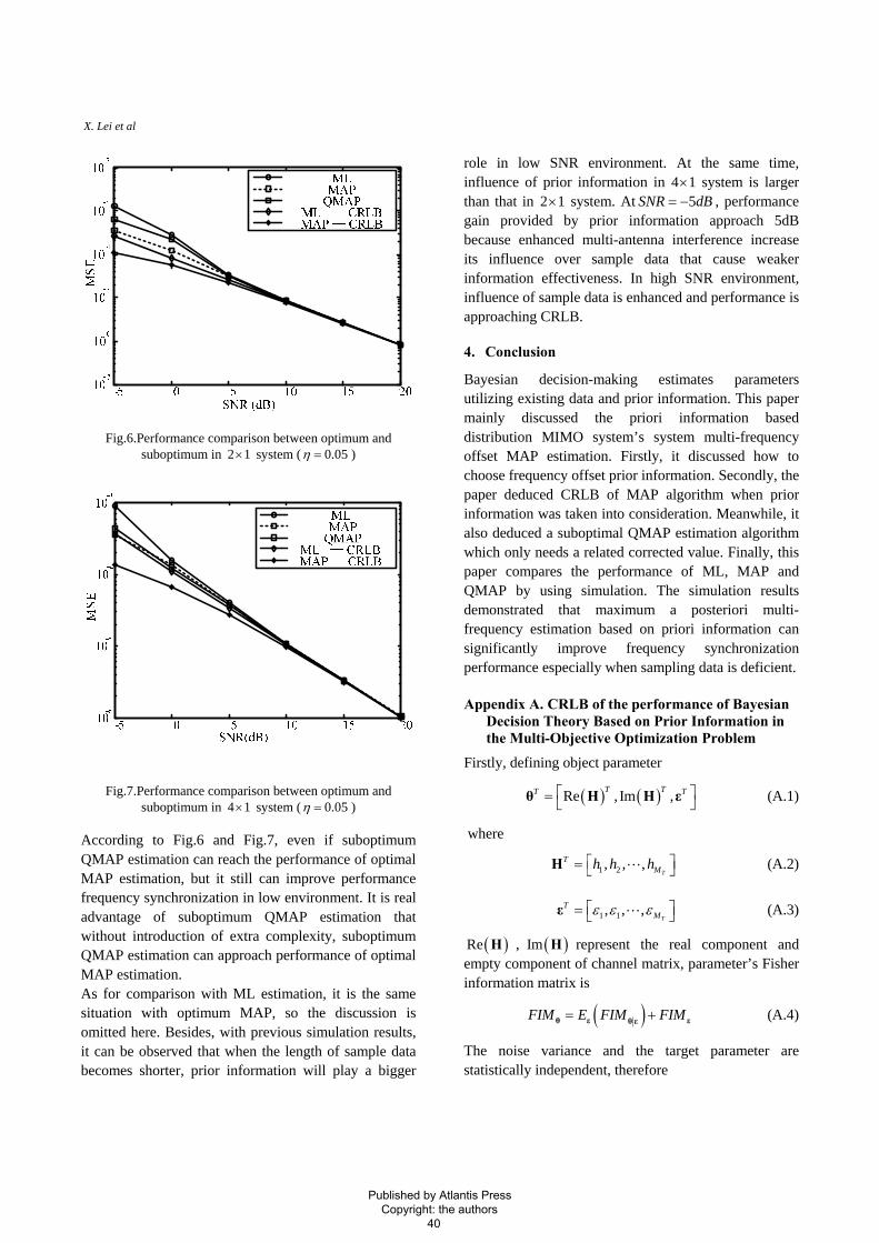
Fig.6.Performance comparison between optimum and

suboptimum in 2 system (1× 0.05η = )

Fig.7.Performance comparison between optimum and suboptimum in 4 system (1× 0.05η = )

According to Fig.6 and Fig.7, even if suboptimum QMAP estimation can reach the performance of optimal MAP estimation, but it still can improve performance frequency synchronization in low environment. It is real advantage of suboptimum QMAP estimation that without introduction of extra complexity, suboptimum QMAP estimation can approach performance of optimal MAP estimation. As for comparison with ML estimation, it is the same situation with optimum MAP, so the discussion is omitted here. Besides, with previous simulation results, it can be observed that when the length of sample data becomes shorter, prior information will play a bigger

role in low SNR environment. At the same time, influence of prior information in 4 system is larger than that in 2

1×1× system. At , performance

gain provided by prior information approach 5dB because enhanced multi-antenna interference increase its influence over sample data that cause weaker information effectiveness. In high SNR environment, influence of sample data is enhanced and performance is approaching CRLB.

5SNR dB= −

4. Conclusion

Bayesian decision-making estimates parameters utilizing existing data and prior information. This paper mainly discussed the priori information based distribution MIMO system’s system multi-frequency offset MAP estimation. Firstly, it discussed how to choose frequency offset prior information. Secondly, the paper deduced CRLB of MAP algorithm when prior information was taken into consideration. Meanwhile, it also deduced a suboptimal QMAP estimation algorithm which only needs a related corrected value. Finally, this paper compares the performance of ML, MAP and QMAP by using simulation. The simulation results demonstrated that maximum a posteriori multi-frequency estimation based on priori information can significantly improve frequency synchronization performance especially when sampling data is deficient. Appendix A. CRLB of the performance of Bayesian

Decision Theory Based on Prior Information in the Multi-Objective Optimization Problem

Firstly, defining object parameter

( ) ( )Re , Im ,θ H H εT TT T⎡ ⎤= ⎣ ⎦ (A.1)

where

1 2, , ,HT

TMh h h⎡ ⎤= ⎣ ⎦ (A.2)

1 1, , ,εT

TMε ε ε⎡ ⎤= ⎣ ⎦ (A.3)

( )Re H , ( )Im H represent the real component and empty component of channel matrix, parameter’s Fisher information matrix is

( )θ ε θ ε εFIM E FIM FIM= + (A.4)

The noise variance and the target parameter are statistically independent, therefore



( ) ( ) ( )1

,2Re ωθ ε

u θ u θC θ

H

i ji j

FIMθ θ

−⎡ ⎤∂ ∂⎡ ⎤ = ⎢⎣ ⎦ ∂ ∂⎢⎣ ⎦

⎥⎥

(A.5)

( )ωC θ Represents covariance matrix of noise,

( )u θ y ω= − (A.6)

furthermore

( )( ) ( ) ( )( ) ( ) ( )( ) ( ) ( )

2

Re Im Im2 Im Re Re

Im Re Reε θ ε

U UU U T

T T VT T

E FIMσ

⎡ ⎤− −⎢ ⎥

= ⎢ ⎥⎢ ⎥−⎢⎣

T

⎥⎦

0H

H

}

⎥⎥⎦

(A.7)

Where,

ε εU Z ZH= (A.8)

02 ε εT Z DZ HHπ= (A.9)

2 204 ε εV H Z D ZH Hπ= (A.10)

( )0H diag= (A.11)

{1,2, ,D diag N= (A.12)

and

(A.13)

[ ] [ ] [ ][ ] [ ] [ ]

[ ] [ ] [ ]

1 2

1 2

1 2

22 21 2

44 41 2

22 21 2

1 1 1

2 2 2εZ

MT

T

MT

T

MT

T

jj jM

jj jM

j Nj N j NM

x e x e x e

x e x e x e

x N e x N e x N e

πεπε πε

πεπε πε

πεπε πε

⎡ ⎤⎢ ⎥⎢ ⎥

= ⎢ ⎥⎢ ⎥⎢⎢⎣

Additionally, the second part of (A.4) can

( )2

ε ε εθ θTFIM E L

⎛ ⎞∂= − ⎜ ∂ ∂⎝ ⎠

⎟ (A.14)

Where,

( ) ( )lnεL p= ε (A.15)

is logarithm probability density function of frequency offset prior information, there are the last TM non-zero elements in the diagonal of matrix εFIM . As

(A.16) ( ) 1 = θθCRB FIM −

( )εCRB of frequency offset can be obtained by matrix decomposition of 1

θFIM −

( ) ( )1

12

2 Reε V T U T RHCRBσ

−−⎧ ⎫= − +⎨ ⎬

⎩ ⎭(A.17)

where，

( ){ }1 2

2 2 2 1 / ,1/ , ,1 /

R ε ε

MTT T

T

M M

E

diag ε ε εσ σ σ×

=

=(A.18)

According to (A.16)， CRLB with prior information adds one term R and because is diagonal positive Rdefinite matrix, theoretically MAP estimation based on prior information can be proved better performance, since Eq. (A.18) always holds

( ) ( )1 1

1 1 12 2

2 2Re ReV T U T R V T U TH H

σ σ

− −− − −⎧ ⎫ ⎧ ⎫− + < −⎨ ⎬ ⎨ ⎬

⎩ ⎭ ⎩ ⎭ (A.19)

Acknowledgment

This work was supported by the National Science Foundation of China under Grant number 60602009 61032002 and 71001075, “863” Project under Grant No. 2009AA01Z236 and No.2008AA04A107, Chinese Important National Science & Technology Specific Projects under Grant 2009ZX03005-003. References

1. R. Etxeberria, P. Larranaga., Global optimization using Bayesian networks[C], The 2nd Symposium on Artificial Intelligence, Habana: CIMAF Press, 1999:332-339.

2. M. Pelikan,D. E. Goldberg and Cantu Paz E. BOA, The Bayesian optimization algorithm[C], Proceedings of the Genetic and Evolutionary Computation Conference. San Mateo: Morgan Kaufmann Publishers, 1999:525-532.

3. H. Müehlenbein, T. Mahnig and A. O. Rodriguez, Schemata, Distributions and graphical models in evolutionary optimization[J], Journal of Heuristics, 1999,(5):215-247.

4. Q Zhang, H Muhlenbein., On the convergence of a class of estimation of distribution algorithms[J], IEEE Trans. on evolutionary computation, 2004, 8(2):127-135.

5. D Heckerman, D Geiger and D M. Chickering, Learning Bayesian Networks: The combination of knowledge and statistical data[J], Machine Learning, 1995, 20(3):197-243.

6. M. Pelikan, K. Sastry, Fitness inheritance in the Bayesian Optimization Algorithm[C], Genetic and Evolutionary


X. Lei et al

Computation Conference(GECCO), Heidelberg: Springer Berlin, 2004:48-59.

7. R. Srinivasan., Distributed radar detection theory[C], Proceedings of the Institute of Electronical Engineers(PI F), 1986, 133(1):55~60.

8. I. Y. Hoballah, and P. K. Varshney., Distributed Bayesian signal detection[J]. IEEE Trans. on Information Theory, 1989, 35(5):995~1000.

9. A. Assenza, M. Valle and M. Verleysen, A comparative study of various probability density estimation methods for data analysis[J], International Journal of Computational Intelligence Systems, 2008, 1-2:188- 201.

10. G. Kong, D. Xu and J. Yang, Clinical decision support systems: a review of knowledge representation and inference under uncertainties[J], International Journal of Computational Intelligence Systems, 2008, 1-2:159 – 167.

11. Y. Liu, J. Huang, A novel fast multi-objective evolutionary algorithm for QoS multicast routing in MANET[J], International Journal of Computational Intelligence Systems, 2009, 2-3: 1875-6883.

12. W.A. Hashlarmoun, and P.K. Varshnery., An approach to the design of distributed Bayesian decision structures[J]. IEEE Trans. on Systems, Manm and Cybernetics, 1991, 21(5):1206-1210.

13. Y. Zhang, H. Chen., Bayesian Statistics Conclusion [M]. Publishing House of Science, 1991

14. Z. Zhang, W. Zhang, C. Tellambura., Robust OFDMA uplink synchronization by exploiting the variance of carrier frequency offsets[J]. IEEE Trans. on Vehicular Technology, 2008, 57(5):3028-3039.

15. T. Bayes, An essay towards solving a problem in the doctrine of chances[J] ， Philosophical Trans. of the Royal Society of London, 1763, 53:370-418.; reprinted in Biometrike, 1958, 45:293-315.

16. Q. Xu, S. Lv, Probability and Mathematical Statistics[M], Higher Education Press, July 2004.

17. P. A. Parker, P. Mitran and D. W. Bliss, et al. On bounds and algorithms for frequency synchronization for collaborative communication systems[J]. IEEE Trans. on Signal Processing, 2008, 56(8):3742-3752.

18. Q. Wang, X. Lei and J. Du, et al. A novel MAP estimation algorithm for multiple frequency offsets in distributed MIMO system[C], IEEE Wireless Communication, Networking and Mobile Computing, 2009.05,page:1-4.

19. Q. Wang, X. Lei and Y. Xiao et al. A Quasi-MAP estimation algorithm for multiple frequency offsets in distributed MIMO system[C], the First International Conference on Wireless Communications and Signal Processing (WCSP), 2009.11,page:1-5.

20. The-Hanh Pham, Nallanathan A. and Y. Liang. Joint channel and frequency offset estimation in distributed MIMO flat-fading channels[J]. IEEE Trans. Wireless Commun., Feb. 2008, 7(2): 648 – 656.


application of bayesian decision theory based on prior

Documents